Operational deployment of LiDAR derived information into softwood resource systems

PROJECT NUMBER: PNC305-1213 FEBRUARY 2015

RESOURCES

This report can also be viewed on the FWPA website

www.fwpa.com.au FWPA Level 4, 10-16 Queen Street,

Melbourne VIC 3000, Australia T +61 (0)3 9927 3200 F +61 (0)3 9927 3288

E info@fwpa.com.au W www.fwpa.com.au

Operational deployment of LiDAR derived information

into softwood resource systems

PNC305-1213

Prepared for

Forest & Wood Products Australia

by

Jan Rombouts, Gavin Melville, Amrit Kathuria Brian Rawley and Christine Stone

Forest & Wood Products Australia Limited Level 4, 10-16 Queen St, Melbourne, Victoria, 3000 T +61 3 9927 3200 F +61 3 9927 3288 E info@fwpa.com.au W www.fwpa.com.au

Publication: Operational deployment of LiDAR derived information into softwood resource systems Project No: PNC305-1213 This work is supported by funding provided to FWPA by the Department of Agriculture (DA). © 2015 Forest & Wood Products Australia Limited. All rights reserved. Whilst all care has been taken to ensure the accuracy of the information contained in this publication, Forest and Wood Products Australia Limited and all persons associated with them (FWPA) as well as any other contributors make no representations or give any warranty regarding the use, suitability, validity, accuracy, completeness, currency or reliability of the information, including any opinion or advice, contained in this publication. To the maximum extent permitted by law, FWPA disclaims all warranties of any kind, whether express or implied, including but not limited to any warranty that the information is up-to-date, complete, true, legally compliant, accurate, non-misleading or suitable. To the maximum extent permitted by law, FWPA excludes all liability in contract, tort (including negligence), or otherwise for any injury, loss or damage whatsoever (whether direct, indirect, special or consequential) arising out of or in connection with use or reliance on this publication (and any information, opinions or advice therein) and whether caused by any errors, defects, omissions or misrepresentations in this publication. Individual requirements may vary from those discussed in this publication and you are advised to check with State authorities to ensure building compliance as well as make your own professional assessment of the relevant applicable laws and Standards. The work is copyright and protected under the terms of the Copyright Act 1968 (Cwth). All material may be reproduced in whole or in part, provided that it is not sold or used for commercial benefit and its source (Forest & Wood Products Australia Limited) is acknowledged and the above disclaimer is included. Reproduction or copying for other purposes, which is strictly reserved only for the owner or licensee of copyright under the Copyright Act, is prohibited without the prior written consent of FWPA. ISBN: 978-1-925213-07-2 Researcher/s: Gavin Melville, Amrit Kathuria & Christine Stone (NSW Department of Primary Industries) Jan Rombouts (ForestrySA) Brian Rawley (Silmetra P/L) Final report received by FWPA in February, 2015

i

Acknowledgements The authors gratefully acknowledge the guidance received from the Project Steering Committee (Mike Sutton, Forestry Corporation of NSW; Jim Ohehir, Forestry SA; Don Aurik, Timberlands Pacific; Kevin Cooney, HQ Plantations and Andrew Lyon, WA Forest Products Commission) in particular, from the Committee Chairman, Glen Rivers (HV Plantations and OneFortyOne). The authors also acknowledge the contributions from: Russell Turner (Remote Census) for the simulated tree dataset used for the tree count algorithm and for his robust discussions on the advantages of tree level analysis; Andrew Haywood for his contribution to the project workshop held 13 June 2013 and all the company representatives on the Project Technical Committee. In addition to the financial support from FWPA, this project was possible because of cash and/or in-kind contributions from NSW Department of Primary Industries, ForestrySA, HV Plantations; Forestry Corporation NSW; Timberlands Pacific; HQ Plantations, Forest Products Commission, Silmetra (NZ) and Foresense PL.

ii

Executive Summary In late 2012 six softwood companies agreed to support a FWPA project focused on the operational deployment of LiDAR derived information into softwood resource systems. The six participating companies were: the Forestry Corporation of NSW; the Forest Products Commission (WA); ForestrySA (FSA); Hancock Victoria Plantations (HVP); Hancock Queensland Plantations and Timberlands Pacific. Building on an earlier FWPA project (“Adoption of new airborne technologies for improving efficiencies and accuracy of estimating standing volume and yield modelling in Pinus radiata plantations”, PNC058-0809) the project set out to develop a LiDAR based inventory solution capable of producing information outcomes that are equivalent to those of existing resource assessments, while demonstrating cost-effectiveness and feasibility of integrating the new solution with existing systems without loss of capabilities. In June 2013 a workshop was held to discuss preliminary results achieved by researchers. At this workshop the key decision was made to adopt a methodology based on nearest neighbour plot imputation on the grounds that it offers the clearest pathway for system integration and permits internally consistent estimation of multiple commercially important resource attributes. At this workshop it was also decided that an operational prototype was to be a key outcome of the project. The workshop decisions helped to focus work on five subject areas: (1) analytical techniques to extract individual tree attributes from LiDAR point clouds, (2) development and evaluation of nearest neighbour imputation models, (3) optimisation of field sampling designs, (4) building of an operational prototype and (5) overall evaluation of the solution, including financial analysis. Three methods for estimation of tree stocking were developed using operational LiDAR point cloud data. The three methods differ in terms of the input data they require and the outputs they produce. The Individual Tree Detection (ITD) method requires field plot data that include measurements of the coordinates of trees. These data are needed to calibrate a model that is used to predict whether maxima in the canopy surface are tree tops or not. This method produces tree maps and individual tree heights. The other two methods - Regression and Variable Window Size (VWS) - do not require tree coordinates in plot data. The Regression method only generates estimates of tree stocking while the VWS method also generates tree locations. Depending on which input data are available and the outputs that are of interest, one of these methods may be selected. The tree maps generated using the ITD and VWS method had high consistency with the manual and visual interpretations. Tree maps are a stand-alone information product that may be used for multiple applications. Further research is needed to examine how plot variables derived from tree maps and individual tree analysis may assist plot imputation. Nearest neighbour plot imputation models were developed and evaluated for two datasets contributed by FSA and HVP. A list of 120 candidate predictor variables was proposed and two alternative methods for predictor variable selection were compared for each of three variants of the nearest neighbour technique. Both stepwise variable selection and genetic algorithms were effective in identifying subsets of variables that produced models with improved predictive performance. These variable selection methods were built into the operational prototype. Detailed analysis of the selected models demonstrated strong predictive behaviour for commercially important forest metrics such as saw log volumes (V20 and Saw 20+). Predictions were weaker for products that were at the extremes of the sawlog size distribution (sawlog with small end diameter greater than 40 cm) or that were strongly influenced by tree form (pulp roundwood). Models predicted diameter distributions fairly closely indicating imputation of plots that were truly representative of the forest at the point of imputation. The models were applied to generate maps of the resource attributes of interest. Imputation outcomes were analysed with respect to geographic origin, age and site quality of imputed plots.

iii

Plot imputation methods require a reference sample of field plots to operate. Alternative methods for selecting this reference sample (random sampling, space filling, grid, systematic, stratified, balanced sampling and locally balanced sampling) were considered. These methods were tested using resampling techniques and in most cases improved efficiencies were recorded compared to random sampling. Some methods (e.g. locally balanced sampling) are highly efficient at an estate level, and while less efficient for small areas such as planning units, they are superior to simple random sampling. Sampling methods are a topic of intense research internationally. The locally balanced sampling strategies, which have recently been published, have only been partially examined by this project so far. These new methods may surpass all the alternative methods which have previously been used. Further research is therefore called for. Until such time a simple method that combines some form of stratification (age, stand history) and grid or random sampling may be recommended. Such a method has the advantage of generating a sample that can be used for traditional design based estimation. LiDAR data do not need to be available at the time of sample design and grid sampling is familiar to inventory contractors. In terms of sample size, large samples (n=1,000) gave RMSE values of around 0.3% for the surrogate variable mean quadratic height (mqh) across the FSA study sites (34,000 plots) and around 2.9% over a small planning unit (125 plots). Small samples (n=50) gave RMSE values of around 1.1% across the entire estate and around 4.3% over the small planning unit. The project implemented a fully operational prototype of a LiDAR based nearest neighbour plot imputation system and made this available to participating companies. It comprises all necessary data processing steps from normalisation of LiDAR data to generation of maps, and allows for data flows to and from other corporate systems such as GIS and growth and yield prediction systems. It is highly modular in structure, command line based (suitable for batch processing) and written in a widely used programming language (R). It leverages existing commercial or freeware tools wherever possible. Trials with the HVP dataset show that processing times are reasonable even with standard PC hardware. The final part of the report evaluates LiDAR based plot imputation from three angles: information outcomes, technical feasibility and cost-effectiveness. The project demonstrated that imputation models possess strong predictive capabilities for many commercially valuable parameters, appear robust and produce predictions that make sense. Since models are central in a model-based inventory system this provides confidence that a LiDAR based inventory system will be able to match the accuracy of conventional systems. There appears to be further potential for model performance enhancement through optimising of systems of sample selection and use of predictors derived from individual tree analysis. LiDAR based inventory generates new types of information products such as tree maps and maps showing the spatial variation of the information of interest. The operational prototype demonstrated that a LiDAR based inventory solution can be integrated with an existing resource planning infrastructure. In fact it can co-exist with existing inventory approaches. The greatest challenge is the development of new skills (R, Lastools, batch processing, model development) should a company chose to perform data processing in-house. The cost profile of LiDAR based forest inventory is scale dependent. This is because LiDAR data acquisition costs depend on the area and fragmentation of the survey area. Moreover, the number of required reference plots is not directly proportional to the survey area: more plots are needed per unit of area for small surveys than for large surveys to achieve the same precision. Financial analysis showed that scenarios where inventories are refreshed annually are only marginally cost-effective. Scenarios where surveys take place every two to three years however were clearly cost-effective. This financial analysis ignores price trends which in the case of LiDAR data are favourable owing to rapid technical advancements in all aspects of data acquisition. It also ignores the emergence of photogrammetric point clouds as an alternative to LiDAR point clouds, or the advancements in unmanned airborne platforms which may change the cost equation of small projects (see Appendix for a discussion of alternative data sources for forest assessment).

iv

Table of Contents Acknowledgements .................................................................................................................................. i

Executive Summary ................................................................................................................................ ii

1 Introduction ..................................................................................................................................... 1

2 Preliminary work: selecting a methodology ................................................................................... 3

3 Research strategy ............................................................................................................................ 6

4 Use of LiDAR point cloud data to improve tree count accuracies. ................................................. 8

4.1 Introduction ............................................................................................................................. 8

4.2 Approach taken for individual tree detection using LiDAR point cloud data......................... 9

4.2.1 Introduction ..................................................................................................................... 9

4.2.2 Step 1 Model Development/Calibration.......................................................................... 9

4.2.3 Identification of the trees in the area of interest ............................................................ 11

4.3 Model development for individual tree detection using simulated data ............................... 14

4.3.1 Simulated Forest data .................................................................................................... 14

4.3.2 Statistical Methods ........................................................................................................ 14

4.3.3 Results ........................................................................................................................... 15

4.4 Individual tree detection algorithm using Green Hills SF data. ............................................ 16

4.4.1 Introduction ................................................................................................................... 16

4.4.2 Statistical Methods ........................................................................................................ 16

4.4.3 Results ........................................................................................................................... 16

4.4.4 Conclusions ................................................................................................................... 18

4.5 Predicting stocking using LiDAR point cloud data from ForestrySA. ................................. 20

4.5.1 Introduction ................................................................................................................... 20

4.5.2 Data ............................................................................................................................... 20

4.5.3 Statistical Methods ........................................................................................................ 21

4.5.4 Results ........................................................................................................................... 22

4.5.5 Conclusions ................................................................................................................... 31

4.6 Predicting optimal window size for estimating stocking and developing tree maps at the plot level using LiDAR point cloud ........................................................................................................ 31

4.6.1 Introduction ................................................................................................................... 31

4.6.2 Method .......................................................................................................................... 31

4.6.3 Results ........................................................................................................................... 31

4.6.4 Conclusions ................................................................................................................... 34

4.7 Overall conclusions comparing the three approaches ........................................................... 34

5 Imputation model development and validation ............................................................................. 36

5.1 Introduction ........................................................................................................................... 36

5.2 Materials ............................................................................................................................... 36

5.2.1 Introduction ................................................................................................................... 36

5.2.2 Field data ....................................................................................................................... 36

5.2.3 LiDAR data ................................................................................................................... 37

5.3 Modelling methods ............................................................................................................... 38

v

5.3.1 Introduction ................................................................................................................... 38

5.3.2 Response variables ........................................................................................................ 39

5.3.3 Identifying candidate predictor variables ...................................................................... 39

5.3.4 Selecting useful predictor variables .............................................................................. 40

5.3.5 Flavours of k Nearest Neighbours ................................................................................ 44

5.4 Results ................................................................................................................................... 44

5.4.1 Variable selection .......................................................................................................... 44

5.4.2 Details of final models .................................................................................................. 46

5.5 Conclusion ............................................................................................................................ 52

6 Reference data collection .............................................................................................................. 53

6.1 Introduction ........................................................................................................................... 53

6.2 Sample selection methods ..................................................................................................... 57

6.3 Sample size ........................................................................................................................... 66

6.4 Conclusion ............................................................................................................................ 68

7 Plot imputation across an area of interest ..................................................................................... 73

7.1 Introduction ........................................................................................................................... 73

7.2 Processing options ................................................................................................................ 73

7.3 Plot imputation across the South Australian study sites ....................................................... 74

7.3.1 Examples of imputed information surfaces ................................................................... 74

7.3.2 Location, age and site quality of imputed plots relative to point of imputation ............ 78

7.4 Calculating stand parameters for an area of interest ............................................................. 81

7.5 Growth modelling options .................................................................................................... 84

8 Data processing flows of an operational prototype ....................................................................... 86

8.1 Introduction ........................................................................................................................... 86

8.2 System context ...................................................................................................................... 86

8.2.1 Inputs ............................................................................................................................. 87

8.2.2 Outputs .......................................................................................................................... 89

8.3 Plot Imputation System Overview ........................................................................................ 89

8.3.1 Internal data flows and data stores ................................................................................ 90

8.3.2 Transforms .................................................................................................................... 92

8.4 Alternatives ........................................................................................................................... 94

8.4.1 Yields that depend on the target pixel ........................................................................... 94

8.4.2 Target pixel metrics that depend on the crop ................................................................ 95

8.5 A Prototype implementation ................................................................................................. 95

8.5.1 Software dependencies .................................................................................................. 96

8.5.2 User interface ................................................................................................................ 96

8.5.3 Limitations .................................................................................................................... 97

8.5.4 Operating environment ................................................................................................. 97

8.5.5 Installation and use........................................................................................................ 97

8.6 Use of R scripts ..................................................................................................................... 98

8.7 Data flows ............................................................................................................................. 98

vi

8.7.1 Inputs ........................................................................................................................... 103

8.7.2 Internal data stores ...................................................................................................... 104

8.7.3 Transforms (R Scripts) ................................................................................................ 106

8.7.4 Outputs ........................................................................................................................ 106

8.8 Scalability ........................................................................................................................... 107

8.8.1 Raster size ................................................................................................................... 107

8.8.2 Variance calculation .................................................................................................... 107

8.8.3 Resource use in test case ............................................................................................. 107

8.8.4 Tree Identification Algorithm ..................................................................................... 109

9 Evaluation ................................................................................................................................... 111

9.1 Introduction ......................................................................................................................... 111

9.2 Information outcomes ......................................................................................................... 111

9.3 Technical feasibility ............................................................................................................ 113

9.4 Cost effectiveness ............................................................................................................... 113

9.4.1 Introduction ................................................................................................................. 113

9.4.2 Cost of LiDAR data .................................................................................................... 114

9.4.3 Cost of Field sampling ................................................................................................ 117

9.4.4 Data processing ........................................................................................................... 118

9.4.5 Start-up costs ............................................................................................................... 118

9.4.6 South Australian case study ........................................................................................ 118

9.5 Conclusions ......................................................................................................................... 121

References ........................................................................................................................................... 122

Appendix 1: Alternate approaches to LiDAR-derived Canopy Height Models of softwood plantations. .......................................................................................................................................... 125

1

1 Introduction The technical feasibility of applying LiDAR (also referred to as Airborne Laser Scanning or ALS) data to estimate forest resource inventory variables has been well established overseas (e.g. Næsset, 2002; Maltamo et al., 2006a; Hyyppä et al., 2012) and in Australia (e.g.Rombouts et al., 2010; Stone et al., 2011a;Stone et al., 2011b, Chen and Zhu, 2012; Musk et al., 2012). More recently, attention has been directed at developing affordable protocols enabling the operational implementation of LiDAR technology by forestry companies e.g. (Treitz et al., 2012). In the Nordic countries, for example, the traditional plot based retrieval of inventory parameters is now commonly being replaced by LiDAR-based inventory methodologies. A FWPA Project PNC0508-0809 (Stone et al., 2011b) demonstrated that estimates of key inventory attributes of Pinus radiata could be accurately obtained from modelling LiDAR-derived metrics and their results supported a future focus on operational implementation of this technology in Australia. The application of remote sensing technologies, in particular LiDAR, was identified as a high priority in the 2011 FWPA Investment Plan on Tools for Forest Management. This was confirmed by an initial Scoping Study submitted by Dr Jerry Leech in June 2012 (PRC281-1112). Based on survey results from the major softwood plantation growers in Australia, Dr Leech concluded that although Australian softwood plantation growers had different levels of experience with LiDAR, most wanted to know how this technology could best be deployed within their companies and to focus on late age inventory. Later in 2012, six softwood plantation companies agreed to support the FWPA project (PNC305-1213) presented in this Report. The companies recognized the mutual benefits of a collaborative approach that shared the costs, expertise and outcomes. The six participating companies were: the Forestry Corporation of NSW; the Forest Products Commission (WA); ForestrySA; Hancock Victorian Plantations; Hancock Queensland Plantations and Timberlands Pacific. The two year project titled ‘Operational deployment of LiDAR derived information into softwood resource systems’ commenced on 1 Nov. 2012 and the Final Report was submitted to FWPA on 1 Nov. 2014. The cash invested in the project totalled $257,000, of which $172,000 was received from FWPA. The project was managed by NSW Department of Primary Industries (DPI) and brought together a team of researchers from NSW DPI (Christine Stone, Amrit Kathuria, Gavin Melville), ForestrySA (Jan Rombouts) and Silmetra Limited in NZ (Brian Rawley). This team combined knowledge of commercial softwood management systems with expertise in biometrical theory and programming. This has enabled a blend of novel and established ideas and approaches to be developed but remain compatible with existing systems. The overall project objective was to provide the collaborating companies with analytical and software solutions enabling the operational deployment of LiDAR derived information into their yield regulation systems. The objective was not to produce commercial software but rather make available to the project participants accessible data flow processes that can be interfaced with existing software infrastructure. The companies drafted the following mission statement for the project - “By 1 January 2015 each of the contributing companies will be in a position to have integrated a LiDAR based inventory solution into their resource planning systems such that : It demonstrably produces resource information outcomes that are equivalent to existing outcomes at a lower cost and it demonstrably can be integrated with existing systems at an acceptable cost without loss of capabilities.” In the project proposal, it was acknowledged that because of differences between companies, a modular approach would be taken, whereby each module could either stand alone or be integrated with the other modules, which in turn, could be customised for integration into individual Forest Management Information Systems.

2

Three project modules were identified and involved developing software solutions that utilised LiDAR data in order to:

Optimise the automatic tree crown detection and for accurate tree count estimates. Implement efficient sampling design strategies to reduce the sampling intensity of inventory

plots. Deliver a data workflow prototype based on plot imputation for volume and product yield

estimates. Supporting these software solutions was a cost-benefit analysis undertaken as part of the feasibility assessment of the operational deployment of LiDAR-derived information into the yield regulation systems. The techniques and solutions developed in this report were developed for airborne LiDAR point cloud data. They should be at least partially transferable to other types of airborne point cloud data, for example those derived from digital imagery. Testing of photogrammetric point clouds for forest assessment could not be accommodated in this project. Appendix 1 provides a report on the state-of-the-art suggesting that this data type warrants closer examination.

3

2 Preliminary work: selecting a methodology At a workshop in June 2013, attended by project staff, stake holders and external experts, the preliminary results of the project were reviewed. The workshop reached a consensus that the methodology most likely to achieve project objectives was that of nearest neighbour plot imputation. Description of nearest neighbour plot imputation Figure 2.1 illustrates how nearest neighbour plot imputation works:

1. Compiling a reference dataset: Nearest neighbour plot imputation is a statistical learning technique. The system learns from a reference dataset, also called the training data. The compilation of this reference dataset is integral part of the imputation process. In a forest inventory context the reference dataset consists of a set of inventory plots in which all the forest attributes of interest (the response “Y”) have been measured (i.e. BA, volume, stocking, product volumes). For each of these inventory plots a set of coincident LiDAR metrics and ancillary variables such as age and thinning history have been measured. These are the predictors “X”. The “X” are also referred to as “features”.

2. Developing a nearest neighbour imputation model: The data in the reference dataset are analysed to select the X that are most effective to predict the set of Y. To be effective as predictors in the imputation model the X must have some explanatory power with regard to the Y and must be known across the survey area. In the example of Figure 1 a strong linear relationship exists between the X and Y. Many types of relationships can be effective. Multiple Y can be simultaneously related to multiple X in the same model. Some nearest neighbour variants (i.e. based on random forests) allow mixing of continuous and categorical predictors.

3. Impute plots using the imputation model. Given a set of X values at a survey location of interest the calibrated imputation model will retrieve from the reference data base the plot(s) with the most similar set of reference X values, i.e. the nearest neighbour in feature space. The plot with most similar set of X is then imputed at the location. Since X and Y are correlated the Y of the imputed reference plot are likely to be similar to the unknown Y at the location of imputation.

Properties of nearest neighbour imputation Integration in existing planning systems. A nearest neighbour plot imputation approach can be easily integrated in existing planning systems because the end-product of the prediction process is a set of imputed plots that can be processed as if it were a sample of plots obtained from a conventional sampling process. Existing systems can be used to process the imputed plots and generate yield tables and so on. In other words, the approach is fully compatible with the existing planning system infrastructure of the industry partners participating in the project. Simultaneous and coherent prediction of multiple response variables. The technique permits simultaneous and coherent prediction of multiple response variables. This is a significant asset in a softwood forest inventory context where typically multiple stand variables, in particular the quantities of volumes by product grade, are of interest. Simultaneous prediction of multiple stand variables is more problematic with regression based techniques. Leveraging any useful data sources to assist prediction. Imputation models can make use of multiple data sources (LiDAR, stand records) to improve predictions. Continuous and categorical predictors can be accommodated in the same model.

4

Figure 2.1: Plot imputation

5

Non-parametric models (McRoberts, 2012). Unlike regression models, kNN imputation models do not require valid assumptions regarding distributions of response and predictor variables. This permits a pragmatic approach to model development: if a predictor variable improves prediction outcomes then use it (even if we do not quite understand why the predictor works). Of course, care must be taken to measure the quality of prediction outcomes effectively. Suitable for mapping, small area estimation and inference (McRoberts, 2012). The end-product of a plot imputation process is a gridded information surface. The data of a subset of grid cells can be combined to provide estimates of arbitrary sub-areas of the surveyed extent. Feature space needs to be sampled efficiently. Bias is possible if the feature space is not effectively sampled. In the example shown in Figure 2.1 the nearest neighbour for cells with X greater than 5 will always be the plot with X=5. Predictions for X > 5 will therefore always be Y=16. The relationship between X and Y strongly suggest that for X greater than 5 the Y will be greater than 16, hence for X>5 the imputed Y are likely to be negatively biased. A regression approach in this case would extrapolate the linear pattern observed between X=1 and X=5 to higher values of X and perform better (regression based extrapolation is however not without risk either!). Methods to sample feature space effectively are being researched worldwide, for example Grafström et al. (2014). The challenge of doing so increases as the number of features increases (i.e. the curse of dimensionality, (Magnussen, 2013)). Lack of small-area variance estimators (to calculate confidence intervals )(Magnussen, 2013) . The approaches proposed in the literature are fairly computing intensive and hard to understand. They often make use of resampling techniques. Of all these properties the ease of integration of a plot imputation approach with existing planning systems and the ability to simultaneously predict multiple response variables using a single model carried the most weight. It was recognised that the research to be undertaken under the project would have to address some of the challenges associated with the method, in particular the development of imputation models with an appropriate number of predictors (Chapter 5) and the selection of a sampling design that optimises reference dataset compilation (see Chapter 6).

6

3 Research strategy The first stage of the project had to tackle technical questions arising when attempting to implement a plot imputation inventory system driven by airborne LiDAR data: How to build an effective imputation model? How to sample for an effective reference dataset? Do imputation results make sense? Are predictions sufficiently accurate? Only after these fundamental questions had been addressed was it possible to implement an operational prototype complete with scripts and software tools, either developed by the project or commercially purchased. At the June 2013 workshop the development of such a prototype had been identified as a key outcome of the project. If successful, it would demonstrate technical feasibility and integration with existing planning systems. The final stage of the project was to evaluate LiDAR based inventory of softwood plantations as a solution for softwood growers. This evaluation focused on information content, integration aspects and cost-effectiveness. In parallel with these activities efforts continued to progress alternative analytical strategies to extract individual tree data from the LiDAR point cloud. These data can be used to generate tree maps as a stand-alone product. But they can also be introduced as predictor variables in a plot imputation process. The structure of this report reflects this strategy. Figure 3.1 shows some key questions arising at each of the operational steps in a plot imputation based forest assessment and planning process. Many of these questions have been taken up by the project, if not necessarily in the order shown in Figure 3.1. Most of the chapters are light on discussion. The reader is referred to Chapter 9 for a discussion of research results in the context of an evaluation of LiDAR based inventory.

7

Figure 3.1: Operational steps in a LiDAR based inventory solution

5. Imputation

Imputation parameters? Confidence intervals? Growth modelling? Software?

4. Imputation model calibration

Response variables? Predictor variables? Nearest neighbour method? Prediction accuracy? Software?

3. Field data capture and modelling

Sample selection strategy? Sample Size? Plot size? Plot Location? Software?

2. LiDAR data capture & pre‐processing

Point density? Partitioning of area of interest? Software? Tree maps? 

1. Inventory design and objectives

Frequency? Information outcomes? Precision?

8

4 Use of LiDAR point cloud data to improve tree count accuracies.

4.1 Introduction Individual tree-crown detection methodologies have been have been widely studied but are not widely applied operationally due to the limited accuracy of the applied algorithms, especially when using low density point data (e.g. < 5 points m-2) (Kaartinen et al., 2008; Ke and Quakenbush, 2011; 2012; Vauhkonen et al. 2012). Kaartinen et al., (2012) report that the percentage of correctly delineated trees has ranged from 40% to 93%. In addition, it has generally been claimed that individual tree detection (ITD) methodologies require a higher pulse density compared to plot level based methodologies and hence requires more expensive LiDAR data, as well as being computationally more demanding than area-based tree count estimates. (Vastaranta et al., 2012). However, if individual tree crowns can be recognized accurately, then this approach tends to outperform the area-based methods (Yu et al., 2010). For example, in addition to providing high spatial resolution stem density information, LiDAR derived ITD tree counts also provides true stem height distributions that can be used for accurate product yield estimates (Kaartinen et al., 2012). The most common approach applied to individual tree detection is local maximum filtering (LMF) (Popescu and Wynne 2004; Ke and Quackenbush, 2011). A fixed-window LMF method works well for stands with uniform tree-crown size. However, for stands with varying crown sizes, if the filter size is too small or too large (or search radius when point data is used), errors of commission or omission respectively, occur. Therefore, if there are multiple tree crown sizes, then the moving local maximum filter should be adjusted to an appropriate size that corresponds to the spatial structure found on the lidar image and on the ground. Most ITD methods are highly dependent on the initial settings such as the degree of smoothing applied to the digital canopy height model (CHM) which can significantly affect the overall detection performance of the algorithm. These approaches require prior knowledge on the potential size and distribution of crown size within the stand. Alternatively, adaptive parameterization in the course of the detection procedure can be applied, ,but this approach requires the application of more complex algorithms. In addition, most reported ITD methodologies commonly detect trees using the lidar-derived canopy height model (CHM), which is a raster image interpolated from LiDAR points depicting the top of the vegetation canopy. Deriving window sizes from raster data has the limitation of restricting the window sizes to 3x3 or 5x5 etc. More recently new methods to detect (and segment) individual trees directly from the 3D ‘cloud’ of LiDAR points have been proposed (e.g. Li and Guo 2012; Wallace et al., 2014). Three methods have been developed for tree density estimation. The individual tree detection, we need tree level data for model development/calibration and it produces tree maps with tree location, height of the trees and possibly the crown radius (we did not have the crown width measurements so we can compare these values). The second method (regression based) does not require tree level information, it only requires plot level no of trees. It produces the number of trees at the plot level. The third method, ‘variable window size’ again does not require data at the tree level we just use the information at the plot level but the advantage over the second method is that it gives a tree map. 1) In current investigation we have developed a novel methodology for accurate tree detection (Individual Tree Detection (ITD)) using operational point cloud data. In this approach we predict the probability of a LiDAR point being a tree top based on a set of focal statistics (local neighborhood of trees in terms of tree crown size, density and clustering), variable based on maxima window and non LiDAR variables such as age and thinning. As a result we can create tree maps for each plot specifying plot locations and height each tree. In an area-based imputation approach (e.g. Sections 5, 6, 7, and 8 of this Report), ITD derived tree counts can be handled as an auxiliary predictor variable in a similar manner, for example, as stand age.

9

2) Use of regression models for the stand density estimation are really popular (Næsset 2002, Hudak et al, 2006 and Yu et al. 2010). Most of these methods use the LiDAR metrics and the non LiDAR variables as the predictor variables. We have used the LiDAR maxima identified from the lidar point cloud data as another set of variables that can be used as the predictor variables for predicting the number of trees per plot. Three regression models using various combinations of field, LiDAR metrics and maxima variables are tested along with another model using the Random Forest algorithm. 3) Variable window size has been applied using the CHM raster data derived from the Green Hills LiDAR dataset (FWPA PNC058-0809; Stone et al., 2011). The disadvantage of raster data is that the window size can only be in steps of 3x3 or 5x5 and so on. Point cloud data is used to develop variable window size method to estimate the number of trees at the plot level. This method is not limited by the restricted number of window sizes. The method provides a tree map identifying the location and height of each tree in the plot. The LiDAR metrics and non LiDAR variables are used as the predictor variables for predicting optimal window size at the plot level. This window size is specific to the plot and maximas identified at this window size give the location and height of the trees. This method is not as precise as the individual tree detection method (ITD) as the window size is chosen at the plot level and not at the tree level (as in ITD) but the advantage is that the tree level data is not required for model calibration.

4.2 Approach taken for individual tree detection using LiDAR point cloud data 4.2.1 Introduction This section outlines the steps and the variables needed to implement the individual tree detection methodology developed using LiDAR point cloud data in pine plantations. It is a two-step process where in step 1 the reference plot data and the corresponding LiDAR point cloud data is used to develop the model and then in second step the model developed in step 1 is applied to the area of interest to develop a tree map, which lists the position and the height of each tree for the specified area. 4.2.2 Step 1 Model Development/Calibration Sample for model development/calibration A good representative sample of plots called the reference plots is selected using an appropriate sampling strategy (refer to Chapter 6). The location coordinates of each tree need to be accurately obtained using a dGPS. Tree heights are also measured in the plots ,although height of the trees is not needed for the tree detection but is used to compare the height distribution of actual trees and the predicted trees. The following three sets of variables (2 derived from the LiDAR point cloud data and 1 non LiDAR variables such as age and thinning) are used as predictor variables: LiDAR Point cloud data Appropriately processed and checked LiDAR data with normalised height values (normalising is the recalculation of LiDAR heights above sea level to heights above the Digital Elevation Model i.e. ground-level) is used for all the LiDAR related variables. The LiDAR data corresponding to the reference plots (include a 5m buffer around the plots for the edge trees) is used for LiDAR maximas and LiDAR focal statistics calculations.

1. .Maximas For each plot, the first step is to filter out all the points <2m. Then, for each point in the point cloud, maximas at 0.5m were identified (the highest point in 0.5m radius circle). The rest of the LiDAR points can be discarded at this initial data thinning stage and we work with only this subset of data. Each of the 0.5m maximas is tested to see if it is a maximum within a series of increasing window sizes i.e. within a 1m, 1.5m, 2m,..5m radius circles.

10

We create a variable called maxima from the maximas file created above. This is the maximum size of the window in which the point is identified as a maxima, e.g. if a point is identified as maxima with window size 0.5m and no other window size, then the maxima value for that variable is 0.5, but if this was a maxima point for a window size 3.5m but not for 4m then the value for this variable is 3.5. This variable is converted to a factor variable (maximaf).

2. Focal statistics Using the point cloud data the following focal statistics are calculated for every maxima identified in initial 0.5m radius search window. These LiDAR metrics are calculated for an increasing series of specified radii (5m, 10m, 15m) around each 0.5m radius maximium point. The focal statistics at 5m, 10m and 15m are highly correlated and as the crown sizes don’t exceed 5m, therefore for the two datasets that we used it was decided to use only the 5m focal statistics. The following focal statistics are computed: cnt2m = Point count above 2m, hrank = Ranking of the height values for the maxima ptp = % of 0.5m maximas taller than point dtp = Distance to tallest point mdatp = mean distance to tallest 3 points etp = Elevation angle to tallest point meatp = Mean elevation angle to tallest 3 point hsum = Height - sum of all points hmax = Height - Maximum hmin = Height - Minimum hmean = Height - Mean hmode = Height - Mode hmedian = Height - Median hvar = Height - Variance hstd = Height - Standard Deviation hmam = Height - Mean above hmean hskew = Skewness hkurt = Kurtosis hquan0 = 0 percentile height hquan10 = 10 percentile height hquan20 = 20 percentile height hquan30 = 30 percentile height hquan40 = 40 percentile height hquan50 = 50 percentile height hquan60 = 60 percentile height hquan70 = 70 percentile height hquan80 = 80 percentile height hquan90 = 90 percentile height hquan100 = 100 percentile height hrange = Height - Range via hmax-hmean hrelrg = Height - Relative Range via hrange/hmean etphq90=etp5/hquan90 maximaf=factor(maxima) distC1 =0,1 variables, ifelse(mdatp5>4,1,0) distC2 = 0,1 variable, ifelse(dtp5>4,1,0) ptpmdatp = ptp*mdaptp ptphq100 = ptp*hquan100 htGT = 0,1 variable, if the height of the point is greater hmean then 1 otherwise 0.

3. Non LiDAR variables The data available in the GIS layers such as age and thinning status is also used for each plot.

11

Model Development The response variable is whether or not the maxima is a tree top or not, and the dependent variables are the LiDAR maxima related variable maximaf, focal statiscs and the non LiDAR variables, e.g. age and thinning. Logistic regression or (and) random forest were used and compared for modelling. The logistic regression performed better than the random forest so this model was selected. The first step is the identification of the variables that are used as predictor variables. This was done by inspecting the correlations between the variables and then picking the variable from the group of highly correlated variables that make the most biological sense and are easy to interpret in terms of their effect on tree identification. After the initial screening, Varimportance from random forest and step wise variable selection in logistic regression is used for selecting the final set of predictor variables. 4.2.3 Identification of the trees in the area of interest Get the normalised point cloud LiDAR data for the area. Filter any area that is not part of the area of interest (AOI). Then divide the data into manageable tiles. For each of the tiles identify the maxima at 0.5m and discard the rest of the points. Use the 0.5m maxima file to calculate the focal statistics. Calculate the derived variables and get the non LiDAR data available from the GIS layers. Use the model developed in the previous step to identify whether the maxima is a tree or not.

12

Figure 4.1: Model Development: Step 1 of Individual tree identification, model see text for detail.

13

Figure 4.2: Step 2 of Individual tree identification, estimating the number of trees for Area of Interest. See text for detail. 

14

4.3 Model development for individual tree detection using simulated data 4.3.1 Simulated Forest data As accurate tree location data is needed to develop models for the identification of individual trees, only data from the Green Hills (SF) study area used in FWPA PNC058-0809 (Stone et al., 2011) was appropriate. The data sets from HVP and Green Triangle were plot level. For the Green Hills study site, the tree crowns were manually delineated using the LiDAR imagery. The size of plots varied from 0.011 to 0.12 ha and the minimum number of trees from the plots was 11. Given that some of the plot sizes were very small, the effect of edge trees on accuracies was very high. Even if one edge tree was not detected, the accuracy was reduced to 90%. It was therefore, decided to create a simulated forest for the purpose of model development (Russell Turner, Remote Census PL, Morisset, pers. comm.). The trees used for the simulated forest were selected from the LiDAR point cloud data acquired for the Green Hills study. The mean point density for this dataset was 2 pulses m-2. Specifications for the number of stems per hectare were taken from the Forest Corporation NSW recommended silvicultural protocols, i.e. compartments are planted to approximately 1000 stems per hectare (ha), thinned between the ages 13 to 17 years old down to 450-500 stems per ha and then thinned again after about 23 years down to 200 to 250 stems per ha. Most compartments are harvested before 35 years of age. Twenty plots (30m radius) each for unthinned (UT), thinned once (T1) and thinned twice (T2) were created. The LiDAR metrics (maxima and focal statistics, derived variables) using the point cloud data (identified in 4.2.2) were calculated for the 60 simulated forest plots and thinning was included as a non LiDAR variable. The response variable is a 0,1 variable indicating if the identified point is a tree top or not. 4.3.2 Statistical Methods Logistic regression was used to fit the data for the tree tops (Cox & Snell, 1989). As is the case with LiDAR data analysis, there is a large number of predictor variables in the model. A number of the input variables are highly correlated, so a number of variable selection methods were used to select the final set of predictor variables. We used a Spearman’s correlation matrix to reduce the number of predictor variables and remove the potential for multi-collinearity in the models (Chatterjee et al., 2000). When two or more variables were found to have a correlation greater than 0.9, we selected one variable and removed all others. A number of techniques have been developed to reduce the number of variables such as; forward, backward and best subset selection. There are techniques which use p values, R2 values, Akaike information criterion (AIC), Bayesian information criterion (BIC) values as the selection criteria. None of these methods are fool proof and care has to be taken in their application. We used the backward selection method with AIC to select for the predictor variables (Harrell, 2014). The model was fitted and classification tables and Receiver Operating Characteristic Curve (ROC) are used for evaluation of the model. An ROC is a standard technique for summarizing classifier performance over a range of trade-offs between true positive (TP) and false positive (FP) error rates (Sweets, 1988). A ROC curve is a plot of sensitivity (the ability of the model to predict an event correctly) versus 1-specificity for the possible cut-off classification probability values π0 (also called threshold value). It can be interpreted as the percent of all possible pairs of cases in which the model assigns a higher probability to a correct case than to an incorrect case (Agresti, 2013). The classification table, with the number of correct matches, can be used to evaluate the predictive accuracy of the logistic regression model. The estimation accuracies of the models were also compared using the root mean square error (RMSE)

RMSE∑ yı yi ^2

n 

15

and bias

bias∑ yı yi

n 

where n is the number of plots, yi is the observed value of the stand variable y, and yı, is the predicted value. RMSE and bias were calculated in relative terms (RMSE% and bias%), the RMSE and bias values for the stand variable y were divided by their observed mean values. All the analysis was done using R statistical package (R Core Team, 2014). 4.3.3 Results The variables in the final model were, log = cnt2m, hrank + dtp + etp + meatp + hsum + hrelrg + hstd + hskew + hquan10 + htGT +

etphq90 + maximaf + distC1 + distC2 + ptpmdatp + ptphq100 + thin Figure 4.3 is the ROC curve. Area Under the curve is, also referred to as the Index of accuracy is 0.979 (confidence interval 0.9777 - 0.9809). The specificity value is 0.954 and sensitivity 0.905. Table 4.1 summarises the total and predicted number of trees for UT, T1 and T2 plots. As can be seen for the UT and T2 plots the predicted number of trees are very close to the actual trees.

Figure 4.3: ROC curve showing the area under the curve(AUC) and the threshold value of 0.347. The numbers in the brackets are the specificity and sensitivity values respectively. Table 4.1: The total number of trees, predicted number of trees and the %Accuracy (Predicted/Actual*100) for the three silviculture treatments.

No. of Trees UT T1 T2

Actual 5244 2733 1243Predicted 5251 2550 1270% Accurate 100.1% 93.3% 102.2%

16

4.4 Individual tree detection algorithm using Green Hills SF data. 4.4.1 Introduction This is the final step in the development of the method for individual tree detection. The previous section outlines the model development using the 60 plots from a simulated forest. The results were very promising. The variables selected using simulation data were used for the actual Green Hills data (described in Stone et al., 2011). A total of 39 plots were selected from the Green Hill study site in NSW. There were 13 UT, 12 T1 and 14 T2 plots. 4.4.2 Statistical Methods The model used was the same as the simulation study (see section 4.3.2 for details). 4.4.3 Results Summary statistics for the selected plots and trees in the plots is presented in Table 4.2 and Table 4.3. As can be seen from Table 4.2 there is large variation in age for UT plots (11.18 to 28.18). The size of the plots were small, for UT it varied from 0.011 to 0.02ha (number of trees varied from 12 to 22), for T1 from 0.015 to 0.062ha (number of trees varied from 11 to 20), and for T2 the plot areas were 0.045 to 0.12 (number of trees varied from 13 to 21). The range of height values (Table 4.3) is also very large, for UT plots the height values vary from 9.06m to 35.08m. The minimum height for the T1 trees was 6.59 and the maximum 33.86m. This shows the high variability in the Green Hills SF data. Table 4.2: The range of the number of trees, Age and the area of Green Hill Plots

Number of trees Age Area(ha) Treatment Number Min Max Min Max Min Max

UT 13 12 22 11.18 28.18 0.011 0.020 T1 12 11 20 16.18 25.17 0.015 0.062 T2 14 13 21 25.19 30.18 0.045 0.120

Table 4.3: Summary statistics for the height of the trees in the selected plots.

Height(m)

Treatment Number Min Max MeanStandard

Deviation

UT 13 9.06 35.08 19.16 6.06T1 12 6.59 33.86 22.25 4.92T2 14 20.17 34.06 29.85 2.22

Figure 4.4 is the plot of the ROC curve showing the AUC value is 0.988 (confidence interval, 0.9801-0.9903) which indicates that the model can discriminate the treetops from the non-tree tops really well. The specificity value is 0.975 and sensitivity 0.923. The results of the analysis at planning unit level are presented in Table 4.4. As can be seen, the number of observed trees is very close to the number of predicted trees. For these dataset the number of trees in at a the planning unit level varies from 16 to a maximum of 65 due to the small plot size and only a few plots per planning unit. RMSE at the planning unit level is 5.7% and the mean number of trees is 37.9 and bias is -2.4%. This is a very good result given the small plot size, even if one trees is missing, this introduces a 2.7% error. The tree level data represents the trees that are manually identified on the screen so suppressed trees that are under larger trees would be missed i.e. these comparisons are for the dominant and co-dominant trees. For T2’s this is not an issue as most of the trees are either dominant or co-dominant. Also, the impact of missing some trees which are suppressed is very small for most important inventory variables, e.g. BA, Volume etc. Figure 4.5 compares the height distributions for the actual

17

and the predicted trees at the silvicultural treatment level. There is a very good match between the two distributions. Figure 4.6 compares the plots of the manually identified trees and the predicted trees, two plots were selected from the UT, T1 and T2 plots. There is a very good match between the two. Table 4.4: Observed and Predicted trees at planning unit level, Accuracy % is Predicted/Actual No. of trees*100 Planning Unit No. of Trees Predicted Accuracy%

1 20 21 105.0% 2 51 49 96.1% 3 32 30 93.8% 4 24 23 95.8% 5 43 42 97.7% 6 60 54 90.0% 7 65 63 96.9% 8 61 59 96.7% 9 32 32 100.0% 10 25 25 100.0% 11 26 26 100.0% 12 62 60 96.8% 13 29 32 110.3% 15 16 17 106.3%  

Figure 4.4: ROC curve showing the area under the curve(AUC) and the threshold value of 0.367. The numbers in the brackets are the specificity and sensitivity values respectively.  

18

Figure 4.5: Plot of height distribution of the manually identified and predicted trees at the thinning level.  

4.4.4 Conclusions A new method is developed for the detection of individual trees. Simulated data was used for the development of the model. Presence and absence of tree top was used as the response variable and a number of focal statistics, maxima, derived and non LiDAR variables (99 variables) were used as predictor variables in a logistic regression model. One variable was selected from a set of highly correlated variables (correlation >0.9) and then backward selection method using likelihood ratio test was used for variable section. Eighteen variables were finally selected as predictor variables. The method uses the variable window size maximas as the tree tops and the size of the window is based on the focal statistics, maxima, derived and non LiDAR variables such as age and thinning. The model was then fitted using the Green Hills data. The number of trees detected was very close to the actual number of trees in the plots and the height distribution of the actual and the predicted trees were very similar.

19

Figure 4.6: Plot of the manually delineated and the predicted tree tops for six plots two each from UT,T1 and T2. The black stars are the manually identified trees and the red filled triangles are the predicted trees.

20

4.5 Predicting stocking using LiDAR point cloud data from ForestrySA. 4.5.1 Introduction The method of tree detection outlined in the previous sections requires tree level reference plot data. The data for South Australia and HVP were at plot level. Numerous studies have shown the feasibility of LiDAR data for estimating forest inventory variables such as BA, Volume, tree height etc. Many of these studies developed models based on LiDAR-derived variables and non LiDAR variables based on known stand or site descriptors – already discussed in the original Introduction). Past studies have looked variable window size for the estimation of stocking applied using the CHM (e.g. Popescu and Wynne, 2004), however much fewer studies have utilised the normalised point cloud data (e.g. Li et al. 2010). This current investigation attempts to optimise the models for the stocking prediction using the LiDAR data and maximas based on the point cloud data with the window size varying from 0.5m to 6m at 0.25m interval. Four different models were developed, one based on Random Forest and the other three using regression but with different sets of predictor variables. 4.5.2 Data Field Data The data used for analysis consisted of 300 field plots from Forestry South Australia (Supplied by Dr. Jan Rombouts). Each plot size was approximately 0.1ha. The field data collected from each of the plots included stocking at the plot level, this is the response variable for this study. Only age, last operation and year since last operation (which could be available from the GIS layers) were used for the analysis. LiDAR metrics The LiDAR metrics defined in section 5.3.3 were used as predictor variables. These are variables derived from the LiDAR height and density CHM data. Only the first returns data was used for this study. The LiDAR metrics used in the modelling consisted of height percentiles (H10 – H90), the mean, maximum & the minimum height, several metrics describing the LiDAR height distribution through the canopy (skewness, standard deviation , kurtosis) and measures of canopy density such as the percentage of ground returns, proportion of returns <=1m, <=2m, <=5m, <=10m. Also, proportion of returns between (90 -100%, 80-90%, 70-80% ...10-0% ) of maximum height, proportion of points with intensity between (0 - 10% , 10-20%, ..., 90-100% )of maximum intensity.(data supplied by Dr Jan Rombouts, for a description of the variables see table 5.4). Maximas derived from the point cloud data. For each plot a buffer of 10m was used and the LiDAR point cloud data was extracted. For each point within this buffered plot it was determined whether the point was a maxima for 0.5m, 0.75m, 1m, ..., 6m. The points that fall in the plot were then summed to give the number of 0.5m maximas in the plot, no of 0.75m maximas etc. A total of 23 such variables were created: RAD0.5 – total number of 0.5 maximas in the plot RAD0.75 - total number of 0.75 maximas in the plot RAD1.0 - total number of 1.0 maximas in the plot …till RAD6.0. The non LiDAR variables such as age and thinning, the LiDAR metrics and the maximas defined above were used as the predictor variables in the model with stems per hectare as the response variables.

21

4.5.3 Statistical Methods Exploratory Data Analysis Exploratory Data Analysis (EDA) is an approach for data analysis that employs a variety of techniques (mostly graphical) to maximize insight into a data set to uncover underlying structure; extract important variables; detect outliers and anomalies; test underlying assumptions; etc. Histograms, density plots scatter and line plots were used for analysis. Also, summary statistics such as the mean, standard deviation and standard errors were used to summarise the data. Random Forest Random Forests (RF) is Classification and Regression method developed by Leo Breiman that uses an ensemble of classification trees (Breiman, 2001) . Random forest uses both bagging (bootstrap aggregation), a successful approach for combining unstable learners and random selection of the independent variables at each node. Each tree is fully grown, this results in the reduction of tree bias. Also, bagging and random variable selection result in low correlation of the individual trees. The algorithm yields an ensemble that has a number of desirable characteristics such as good accuracy; robustness to outliers and noise; speed; internal estimation of error, strength, correlation and variable importance. Prediction performance of the random forest algorithm is performed using a type of cross-validation in parallel with the training step by using the so-called out-of-bag (OOB) samples. As in a bootstrap sample sampling is done with replacement, approximately one third of all the observations are left out of the bootstrap sample; these observations are called "out-of-bag" (OOB) data. The OOB data are then used to estimate prediction accuracy (Liaw and Wiener, 2002). Multiple Regression (Linear and Non Linear) Multiple linear regression is a statistical technique that uses several explanatory variables to predict the values of a response variable. Every value of the explanatory variable x is associated with a value of the dependent variable y. The population regression line for p explanatory variables x1, x2, ... , xp is defined to be µy=β0 + β1x1 + β2x2 + βpxp. This line describes the change in mean response of the dependent variable with the changes in the explanatory variables. In our ForestrySA dataset there were 300 observations and 109 variables. Overfitting is a term used to describe the situation when there are too many parameters to estimate for the amount of information in the data. Collinearity is another big issue with this data as some of the variables are highly correlated with other variables. For the first model all the LiDAR, maxima variables (RAD0.5, RAD0.75 etc.) and non LiDAR variables defined above are considered as the predictor variables. We used the backward selection method with AIC to select the predictor variables (see section 4.3.2). The second model that was developed was based only on the non LiDAR variables that are easily available and the maximas (RAD0.5, RAD1.0 etc). A third model was developed with selection of variables that were identified as important and then using the variable reduction method such as identifying and picking up one variable from a set of highly correlated variables and then backward selection method on the remaining set of variables. Also, nonlinearity was introduced in the model and generalised additive model was used (Hastie and Tibshirani, 1990, Venables and Ripley, 2002). AIC and significance of non linear terms was used to decide if the non linear terms should be included in the model. Model Assessment and Validation After fitting, the model was tested for four principal assumptions which justify the use of linear regression models for purposes of prediction; linearity, normality, independence of the errors and homoscedasticity (constant variance) of the errors. Residual plots were used to make sure that none of assumptions are violated. Models were validated using boostrap sampling. The bootstrap family was introduced by Efron and is fully described in Efron & Tibshirani (1993). For a given dataset, samples of the same size as the original data set are drawn with replacement. Since the dataset is sampled with replacement the probability of any given instance not being chosen after n samples is (1-1/n)^n ≈ ≈ 0.368. Each

22

bootstrap sample is used for training and then the complete dataset used for prediction accuracy estimation. Accuracy Assessments Model precision was determined using the coefficient of determination (R2). The estimation accuracies of the models were compared using the root mean square error (RMSE) and bias (see section 4.3.2 for detail). All the analysis was done using R statistical package (R Development Core Team, 2014). 4.5.4 Results Data Representativeness The summary for the field data is presented in Table 4.5. The data had a good representation of the different field plot conditions but only four plots were selected from the T4 population which could mean that the estimates from this section could have large variances, and maybe not enough to represent the T4 population. Also, there was only one age-class for this group of plots. The range of basal area and stems per hectare reflects this. Table 4.5: Summary statistics for the field data. The mean values or each variable is listed along with the range in parenthesis.

Plot No of plots Age Stems Per Ha BA Mean Diameter

T1 45 15.7(14-19) 702.6(380-920) 36.3(21.0-44.9) 25.4(21.9-30.4)

T2 107 25.6(22-29) 373.9(150-500) 36.8(22.5-47.7) 35.4(28.9-50.2)

T3 144 29.5(27-32) 260.3(150-340) 33.7(20.5-52.0) 40.4(35.8-47.4)

T4 4 29(29-29) 197.5(180-210) 28.3(26.1-32.13) 42.5(41.4-43.9)

Bivariate Correlations The pair wise plots for some of the variables are presented in Figure 4.7 to show the correlation between the variables. This plot shows that there is very high correlation among h90, h80, h70 and h60. Also for h10 most of the values are sitting on one side and only one value is about 5. This is reflected in the histogram presented in Figure 4.8. Such variables should not be included in the analysis.

23

Figure 4.7: Pairwise scatter plot of h90: h10 LiDAR metrics variable

Figure 4.8: Histogram of h10 LiDAR metrics variable. Random Forest Random Forest (RF) was used with all the variables included in the model. Figure 4.9 is the plot of observed number of trees per plot against the predicted number from the RF. RF explained 91.6% of the variability in the data. The T4 points (blue in colour) appear to be sitting above the 0,1 line, indicating that there is a upward bias in the estimation of these points. The average RMSE at the plot level is 12.6% and the average bias is 0.47%. Table 4.6 presents the plot level and plantation level RMSE and Bias estimates. As can be seen from the table the plot level bias for T4 is 18.7%. The average RMSE at the plantation level is 4.8% and the average bias is 0.82%.

24

Figure 4.9: Scatter plot of the observed and the predicted number of trees using random forest. The colour of the points is the thinning operation. black for T1, red for T2, green T3 and blue T4. Stepwise variable selection The model fitted using a stepwise backward selection using AIC. The model and the coefficients are presented below. The model contains 22 variables and explains 94.6% of the variability in the data. But variance inflation factor (VIF), which quantify the severity of multicollinearity are high for some of the variables indicating presence of collinearity. Figure 4.10 is the plot of observed number of trees per plot against the predicted number from the stepwise model. The average RMSE at the plot level is 11.0% and the average bias is negligible. Table 4.6 presents the plot level and planning unit level RMSE and Bias estimates. As can be seen from the table the plot level bias is negligible for each of the T1:T4 classes. The average RMSE at the planning unit level is 3.8% and the average bias is negligible. The RMSE values from the bootstrap validation are plotted in Figure 4.11 and 4.12 for thinning and planning unit levels respectively. The red line is the median value of the RMSE. The median bootstrap RMSE at the plot level is 11% and at the planning unit level it is 3.8% . Model used: Notrees ~ f(RAD1.5, RAD4.25,lo,kurtosis,d0_10,d10_20,d30_40,d40_50, d50_60, d60_70, d70_80, d80_90, d90_100, i0_10,i10_20,i50_60,i60_70,i70_80,p10m,lmh, lp10m, h70) The number of trees at the plot level (Notrees) is a function of the twenty two variables listed above.

25

Table 4.6: Plot and planning unit level RMSE and Bias estimates for the different models

Plot Level Plantation Level Plots Number RMSE Bias Number RMSE Bias

Random Forest T1 45 11.4 -1.0 4 2.3 -1.0 T2 107 11.8 -0.1 12 4.4 -0.1 T3 144 13.4 0.9 16 4.8 0.9 T4 4 23.7 18.7 1 18.7 18.7 Stepwise Variable selection All Variables T1 45 6.8 0.0 4 1.4 0.0 T2 107 10.9 0.0 12 4.6 0.0 T3 144 12.4 0.0 16 4.0 0.0 T4 4 14.6 0.0 1 0.0 0.0 Field and LiDAR Maxima T1 45 10.7 -0.2 4 2.4 -0.2 T2 107 12.7 0.2 12 5.9 0.2 T3 144 11.8 0.0 16 4.3 0.0 T4 4 3.7 0.0 1 0.0 0.0 Selected Field, Maxima and LiDAR metrics T1 45 9.1 -0.1 4 1.4 -0.1 T2 107 11.0 0.1 12 4.6 0.1 T3 144 11.5 0.0 16 4.4 0.0 T4 4 6.6 0.0 1 0.0 0.0

Figure 4.10: Scatter plot of the observed and the predicted value of number of trees at the plot level from the stepwise model selection using all variables. The colour of the points is the thinning operation. black for T1, red for T2, green T3 and blue T4.

26

Figure 4.11: Histogram plot of the RMSE values at the plot level from the 500 bootstrap samples. The different panels are for the different thinning regimes.

Figure 4.12: Histogram plot of the RMSE values at the planning unit level from the 500 bootstrap samples. The different panels are for the different thinning regimes. Field data and LiDAR point cloud maxima The model fitted using only the field plot data and the LiDAR cloud maxima variables (RAD0.5, RAD1.0 etc.). Interaction terms of the LiDAR maxima and the last operation (lo) variable improved the model fit (lower AIC values). Only four variables: RAD0.5 (total number of plot maximas with

27

radius 0.5) , RAD4.25, age and lo were used for model fitting. The model was fitted using generalized additive models and spline terms were included for RAD0.5, RAD4.25 and age. This simple model explained 92.2% of the variability in the data. Figure 4.13 is the plot of observed number of trees per plot against the predicted number from this model. The average RMSE at the plot level is 11.8% and the average bias is 0.03%. Table 4.6 presents the plot level and planning unit level RMSE and Bias estimates. The average RMSE at the planning unit level is 4.5% and the average bias is 0.03%. The RMSE values from the bootstrap validation are plotted in Figure 4.14 and Figure 4.15 for plot and planning unit levels respectively. The red line is the median value of the RMSE. The spread of the histogram shows the variation in the RMSE and the Bias values for the different bootstrap samples. The values for T4 plots are highly variable, this is expected given the small number of plots in T4 (only 4). The median bootstrap RMSE at the plot level is 12.4% and at the plantation level it is 5.2% Model used: Notrees ~ f( s(RAD0.5, k = 5, by = lo) , s(RAD4.25, k = 5, by = lo) , s(age, k = 5, by = lo)) The number of trees at the plot level (Notrees) is a function of the only four variables listed above. A smoothing spline with 5 degrees of freedom is fitted to RAD0.5, RAD4.25 and age variables. A separate smother is fitted to each of the thinning classes (by=lo).

Figure 4.13: Scatter plot of the observed and the predicted value from the field and LiDAR maxima variables. The colour of the points is the thinning operation. black for T1, red for T2, green T3 and blue T4.

28

Figure 4.14: Histogram plot of the RMSE values at the plot level from the 500 bootstrap samples. The different panels are for the different thinning regimes.

Figure 4.15: Histogram plot of the RMSE values at the plantation level from the 500 bootstrap samples. The different panels are for the different thinning regimes. Field data and LiDAR point cloud maxima and LiDAR metrics The model was fitted using the field data, LiDAR cloud maxima and LiDAR metrics variables. Only the variables that were selected in the previous two models were used. The variables were then checked for multi-collinearity and a step wise manual selection was applied for the selection of the variables. Some variables such as age, thinning and RAD1.5 are forcefully retained in the model. The variables selected for this model are RAD1.5, RAD4.25, age, lo, h80, h30, year since the last operation, pdhLiDAR (lidar based predominant height), and skewness. Interaction terms of the LiDAR maxima and the last operation (lo) variable improved the model fit (lower AIC values). The model was fitted using generalized additive models and spline terms were included for RAD1.5, RAD4.25, h80, h30, skewness

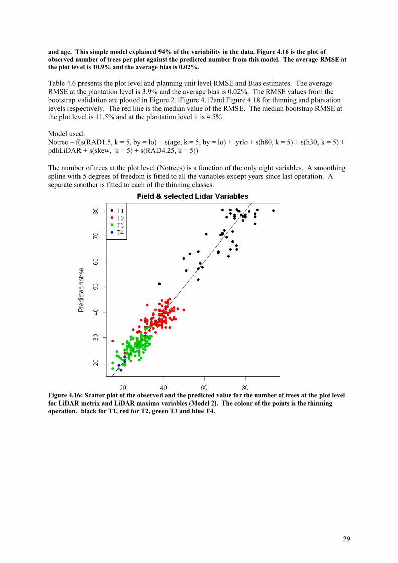
29

and age. This simple model explained 94% of the variability in the data. Figure 4.16 is the plot of observed number of trees per plot against the predicted number from this model. The average RMSE at the plot level is 10.9% and the average bias is 0.02%. Table 4.6 presents the plot level and planning unit level RMSE and Bias estimates. The average RMSE at the plantation level is 3.9% and the average bias is 0.02%. The RMSE values from the bootstrap validation are plotted in Figure 2.1Figure 4.17and Figure 4.18 for thinning and plantation levels respectively. The red line is the median value of the RMSE. The median bootstrap RMSE at the plot level is 11.5% and at the plantation level it is 4.5% Model used: Notree ~ f(s(RAD1.5, k = 5, by = lo) + s(age, k = 5, by = lo) + yrlo + s(h80, k = 5) + s(h30, k = 5) + pdhLiDAR + s(skew, k = 5) + s(RAD4.25, k = 5)) The number of trees at the plot level (Notrees) is a function of the only eight variables. A smoothing spline with 5 degrees of freedom is fitted to all the variables except years since last operation. A separate smother is fitted to each of the thinning classes.

Figure 4.16: Scatter plot of the observed and the predicted value for the number of trees at the plot level for LiDAR metrix and LiDAR maxima variables (Model 2). The colour of the points is the thinning operation. black for T1, red for T2, green T3 and blue T4.

30

Figure 4.17: Histogram plot of the RMSE values at the plot level from the 500 bootstrap samples. The different panels are for the different thinning regimes. The red line is the median RSME.

Figure 4.18: Histogram plot of the RMSE values at the planning unit level from the 500 bootstrap samples. The different panels are for the different thinning regimes.

31

4.5.5 Conclusions Regression methods are very popular in area based tree density estimation. These methods use LiDAR metrics and non LiDAR variables as predictor variables. We have included number of maxima at varying window sizes as another set of variables as predictor variables. All the three regression models used performed really well. The model developed using the field variable such as age and two maxima and last operation variables give very good estimates of plot level and plantation level tree density (12.4% and 5.2%) and used only four variables, whereas the model with twenty two variables produced the lowest RMSE estimates both at plot and plantation levels (11% and 3.8%). Logistic regression and random forest were used for modelling the tree density. Logistic regression performed better than random forest.

4.6 Predicting optimal window size for estimating stocking and developing tree maps at the plot level using LiDAR point cloud

4.6.1 Introduction Variable window size method for estimation of tree density has been applied previously using the Green Hills CHM raster data (FWPA PNC058-0809; Stone et al, 2011). It has been shown that the smaller window sizes of 3x3 or 5x5 are required for the UT plots and bigger window sizes are needed for the T1 and T2 or higher thinning plots. In this section we describe a methodology for predicting variable window size using the point cloud data. In the method developed in section 4.5 we used regression models and random forest methods to predict the number of trees at the plot level. In this section we develop a method to estimate the number of trees at the plot level and create tree maps. This is similar to the individual tree detection method but the window size is chosen at the plot level and not at the tree level, hence the tree level data is not required for model calibration. The FSA data was used for this study. The field data and the LiDAR metrics data are the same as in section 4.5.2, but the resolution for the point cloud maximas is 0.1m instead of 0.25m in section 4.5.2. 4.6.2 Method Random forest method as described in section 4.5.3 above is used for fitting the optimum window size to the set of LiDAR and non LiDAR variables. Point cloud data is used and maximas at plot level are identified for varying window sizes (0.5m to 5.5m in steps of 0.1m). The number of maximas at the plot level is computed for the above mentioned window sizes. The number of maximas at each window size was then compared to the observed number of trees in the plot and the window size which gives the closest value to the observed is taken as the optimum window size. This optimum window size is used as the response variable and the LiDAR metrics and non-LiDAR variables are used as predictor variables to predict the optimum window size for the plot. Once the optimum window size is estimated the number of trees and the tree map can be generated by using the optimum window size with the point cloud data, the maxima locations are the trees. The advantage of this over the individual tree detection method is that there is no need for tree level data for each of the reference plots. But the individual tree detection method is more precise as the size of the window for maxima changes for each tree rather window size changing at the plot level. 4.6.3 Results The minimum number of trees in the plots was 15 and the maximum was 94. The minimum size of the window was 1.6m and the maximum 2.7m. As expected for the plots with last operation as T1 smaller window sizes were predicted and larger window sizes were predicted for the T2 and T3 plots. The %RMSE and %bias at plot level were 13.3% and -1.3% and at planning unit level these values are 5.1% and -2.1%. Table 4.1 below summarises the number of trees at the planning unit level and the predicted number of trees. An accuracy index which is calculated as Predicted/Actual*100 is also presented. Figure 4.19 is the plots of the actual number of trees vs the predicted number of trees at

32

the plot (R2 value 0.91) and planning unit levels (R2 value 0.99) respectively. Figure 4.20 is the plot of the LiDAR point cloud data and the maxima locations using the optimum window size for that plot.

Figure 4.19: Plots of the actual number of trees vs the predicted number of trees at the plot and planning unit levels. The line is a line with 0 intercept and slope 1.

33

Table 4.7: Predicted and the observed trees at planning unit level, Accuracy is Predicted/Actual No. of trees*100.

Planning Unit noTree NtreeP Accuracy

2038102 262 256 97.7%2038112 309 313 101.3%2038201 249 231 92.8%2038202 403 395 98.0%2038210 300 301 100.3%2038401 495 460 92.9%2038402 438 448 102.3%2038407 322 301 93.5%2038408 31 36 116.2%2039301 910 861 94.6%2039306 61 52 85.3%2039801 1126 1111 98.7%2039802 1069 1048 98.0%3018101 309 291 94.2%3018201 184 179 97.3%3018302 108 111 102.8%3018304 102 100 98.0%3018305 180 176 97.8%3018306 511 511 100.0%3018312 59 51 86.4%3018315 108 118 109.2%3018410 97 97 100.0%3018414 196 201 102.6%3018505 209 210 100.5%3018507 500 455 91.0%3018508 617 596 96.6%3018819 183 178 97.3%3018909 379 360 95.0%3018913 340 335 98.5%3018917 124 110 88.7%3019005 560 588 105.0%

3019013 152 153 100.7%

34

Figure 4.20: Plot of the LiDAR point cloud data and the predicted trees. The red triangles denote the location of the tree 4.6.4 Conclusions We have developed a method using random forest for the optimum window size prediction with LiDAR metrics and non LiDAR variables as predictor variables. Optimum window size is the size of the window that would give the best match between the actual number of trees in the plot and the number of maxima at the plot level using the predicted window size. As expected smaller window sizes are predicted for T1, and bigger for T2 and T3 plots. Using the optimum window size the maxima are computed and the coordinates of the maxima identify the tree tops. So along with the number of trees at the plot level, tree maps can also be generated using this method.

4.7 Overall conclusions comparing the three approaches We have developed three methods for tree density estimation; all the methods were shown to produce accurate estimates of tree density. For Individual tree detection (ITD) method, the location coordinates of each tree need to be accurately obtained using a dGPS for model development/calibration and it produces tree maps with tree location, height of the trees and

35

possibly a surrogate for crown diameter (crown width measurements were not available for this study but visual inspection does seem to indicate this). The ITD method was developed using the simulated dataset and tested using data from Green Hills SF ( LiDAR pulse density 2 points m-2). For simulation data (60 plots of 30 m radius) plot level estimates of RMSE% and Bias% were 8.74% and -2.21% respectively. For Green Hills, NSW data, there were 39 plots (13 UT, 12 T1 and 14 T2 plots). These plots were highly variables in terms of tree density and height of trees and the plot sizes were very small making it a challenging dataset, nevertheless, RMSE% at the plot level was 9.59% and bias 0.95%. The RMSE at the planning unit level is 5.7% and bias is -2.4% (the range for the no. of plots per plantation was 1 to 4). As the accurate tree level data is not always available a further two methods were developed; one based on regression of tree density at plot level and the other based on the variable window size for maxima at the plot level. These two methods do not require dGPS located tree level data. The response variables are the number of trees at the plot level. For the regression method, four different models were used, one based on Random Forest (RF), and the other three using regression but with different sets of predictor variables. With these models, for FSA data the plot level RMSE% range from 10.8% to 12.6% with bias % values ranging from 0 to 0.47%. The RMSE% at the planning unit level range from 3.95% to 4.81% with the bias% values ranging from 0 to 0.82%. Tree level maps cannot be generated with this method. The third method called the variable window size method, uses RF for the optimum window size prediction with LiDAR metrics and non LiDAR variables as predictor variables. Optimum window size is the size of the window that would give the best match between the actual number of trees in the plot and the number of maxima at the plot level using the selected window size. The %RMSE and %bias at plot level were 13.3% and -1.3% and at planning unit level these values are 5.1% and -2.1%. So along with the number of trees at the plot level, tree maps can also be generated using this method. The location and the height of each tree in the plot could be predicted from the coordinates of the maximas.

36

5 Imputation model development and validation

5.1 Introduction The imputation model is the engine of the imputation based inventory approach. The function of the imputation model is to retrieve from the reference database the plot(s) that will be imputed at the prediction location based on the similarity of plot features and features observed at the location of prediction. The following paragraphs report the results of research into feature (= predictor variable) selection methods in a nearest neighbour prediction system, and the performance of alternative methods for calculating “nearness” (similarity) in feature space.

5.2 Materials 5.2.1 Introduction The project made use of existing datasets that had to meet following criteria: Availability of relatively high density LiDAR data (at least 4 pulses m-2) A sufficient number (200+) of coincident inventory plots measured shortly after/before LiDAR

data acquisition. Two of the participating forest growers (HVP and FSA) were able to contribute datasets meeting these criteria. 5.2.2 Field data The field data contributed by FSA and HVP were quite different because of the inventory methods applied by either company (see Table 5.1). Table 5.1: FSA and HVP field plot attributes FSA HVP sample selection stratified random square grid no plots 304 236 mean plot area (m2) 1000 330 (75-600) plot location accuracy 6 m "within 20 m" %stdev (TRV) 23.5 63.9 %stdev (N) 44.4 52.4 measurements

DBH yes yes height yes yes stem straightness, branching and defects no yes

planning units 34 29 age range 14-32 10-32 mean age 26.1 17.3 history T1, T2, T3, T4 UT, T1, T2

The smaller plot sizes of the HVP plots result in higher standard deviations of estimates. This is an expected result of smaller plot sizes. However in a LiDAR context one also needs to consider that smaller plot sizes adversely affect the precision of LiDAR predictions models (Gobakken and Næsset, 2008). This is because in small plots, for a given plot location error, the spatial mismatch of LiDAR and field data, will generate proportionally more noise in the relationships between field and LiDAR metrics that underpin the prediction models.

37

By design FSA plots are located more precisely than HVP plots. This should give FSA models an edge, all other things being equal (Frazer et al., 2011). As will be shown in following paragraphs plot imputation makes use of LiDAR metrics derived from the distribution of LiDAR heights in the plots. (Magnussen and Boudewyn, 1998, Rombouts, 2011) have shown that some of these LiDAR metrics are dependent on plot size, while others are not. For this reason, variable plot sizes such as those encountered in the HVP dataset cannot be recommended. A final significant difference between the datasets lies in the distribution of plots by age class (see Figure 5.2). In the FSA dataset plots are concentrated in the older age classes. In the HVP datasets plots are concentrated in the younger age classes. The FSA plots are also characterised by more frequent thinning.

Figure 5.1: Distribution of plots by plantation age class 5.2.3 LiDAR data Table 5.2 shows the acquisition parameters for the FSA and HVP LiDAR datasets. The FSA LiDAR datasets are of a slightly higher density (5.9 versus 3.6 pulses m-2). Either dataset should lend itself quite well to a broad range of analytical techniques, including individual tree analysis techniques.

FSA

age

Fre

quen

cy

15 20 25 30

02

040

608

0

HVP

age

Fre

quen

cy

10 15 20 25 30

020

4060

80

38

Table 5.2: FSA and HVP LiDAR data specifications FSA

Lidar data supplier De Bruin Spatial Technologies System / Sensor ALTM Orion Date of acquisition January 2012 Data format LAS Flying altitude (m ASL) 800m Pulse repetition rate (kHz) 150 kHz Scan pattern zig zag Swath width (m) +/- 250m Scan overlap (%) 25 Maximum scanning angle (0) 15 Beam divergence (mradians) 0.25 Mean footprint diameter (cm) 19 Returns per pulse 1-4 Mean point density - First return only density (m-2) 5.9 Mean point density - First and last returns density (m-2) 8.9 Point density range 3.4-9.2 (in 304 inventory plots) Horizontal accuracy (m) 1σ: 0.5 m Vertical accuracy (m) 1σ: 0.25 m LiDAR classified into ground or non-ground points ground, non-ground, overlap surplus Datum and Projection D_GDA_1994, Transverse_Mercator

HVP Lidar data supplier Photomapping Services System / Sensor Optech ‘ALTM Gemini’ Date of acquisition 13th April 2012 Data format LAS or text point data files Flying altitude (m ASL) 800m Pulse repetition rate (kHz) ? Scan pattern zig zag Swath width (m) 400 Scan overlap (%) 40 Maximum scanning angle (0) + / - 10 Beam divergence (mradians) 0.25 Mean footprint diameter (cm) 24 Returns per pulse 1st through to 4th Mean point density - First return only density (m-2) 3.6 Mean point density - First and last returns density (m-2) 5.6 Point density range 1.0-6.2 Horizontal accuracy (m) ±0.15m @ 1σ Vertical accuracy (m) ±0.15m @ 1σ LiDAR classified into ground or non-ground points Yes (las file) Datum and Projection GDA94 MGAZ55

5.3 Modelling methods 5.3.1 Introduction In developing an effective imputation model methodology decisions need to be made about:

which response variables Y to include in the model; which LiDAR and ancillary metrics to consider as candidate predictor variables X; how to select a subset of predictors to optimise the model; how to calculate nearness in feature space; and how many nearest neighbours to consider

Obviously the objective is to achieve the best overall imputation performance with regard to the response variables (Y). How to measure this also needs to be determined.

39

5.3.2 Response variables Typical Australian softwood resource planning systems generate information about inventory and flows of log products at a stand or estate level. Metrics of interest may include:

Basal area and height Stocking Total Recoverable Volume (TRV) – which is closely related to carbon stocks Volumes by product (grade) and size class mean tree size diameter distributions

The measurements made in HVP and FSA field plots differ significantly. HVP practices overlapping feature inventory which involves detailed mapping of stem attributes such as sweep, branching and defects along the length of each tree stem in the plot. FSA does not practice this type of field cruising and as a result does not directly estimate volumes by product grade (saw, pulp, poles). Instead it applies product models to predict product outturn. To be effective an imputation model must impute plots that provide a good match for multiple response variables at the point of imputation. It is not enough to just predict total tree volume: we are also interested in mean tree volume, basal area, volumes by size classes. One of the strengths of nearest neighbour imputation models is that multiple response variables may be inserted in the model. In this study eight response variables were inserted in the model. Sensitivity analysis suggested that this number was adequate, and perhaps even excessive. (Maltamo et al., 2009) obtained good results for prediction of diameter distributions with 5 response variables. Optimisation of the number of response variables warrants more research because models with numerous response variables are computationally more expensive. Table 5.3 shows the sets of response variables for the FSA and HVP imputation models. These reflect the differences in field cruising methods mentioned earlier. Table 5.3: Response variables used in FSA and HVP imputation models

FSA HVP Response Description Response Description V7 volume to 7 cm SED (*) TRV total recoverable volume V10 volume to 10 cm SED roundwood all non-saw log V20 volume to 20 cm SED Saw 20cm+ sawlog >= 20cm SED V30 volume to 30 cm SED Saw 30cm+ sawlog >= 30cm SED V40 volume to 40 cm SED Saw 40cm+ sawlog >= 40cm SED BA basal area BA basal area SPH stocking per ha SPH stocking per ha mtv mean tree volume mtv mean tree volume (*) SED = Small End Diameter 5.3.3 Identifying candidate predictor variables Predictor variables will only be useful in an imputation model if they have some explanatory power for one or more of the response variables. Identifying a list of candidate predictor variables is an important first step. Much of the so-called “area based” research over the past 30 years has focused on identifying predictor variables that characterise the point cloud enclosed in a small area, i.e. a plot, and are correlated with forest metrics such as basal area, volume, stocking. To name a few significant studies: (Maclean and Martin, 1984), (Nelson et al., 1988), (Magnussen and Boudewyn, 1998), (Næsset, 1997), (Nilsson, 1996), (Holmgren et al., 2003).

40

Many of the variables encountered in the literature have been included in the candidate list of variables shown in Table 5.4. Some studies have reported the use of ancillary variables in nearest neighbour prediction models (Maltamo et al., 2006b). In even-aged softwood plantations the variable age has significant information content and would be expected to be a powerful predictor variable. Thinning status (thinning history) may be significant in estates with regular and frequent thinning regimes such as South Australia. This study also introduced age interaction metrics. Interaction metrics are simply the product of LiDAR metrics and age. Hence three classes of metrics were included in the candidate predictor list:

1. LiDAR metrics: computed based on the height distribution of first and last returns in a plot or gridcell. Metrics based on return intensity were not considered as preliminary analysis suggested they did not add much to imputation performance.

2. Ancillary metrics: variables such as plantation age, site quality, thinning state. 3. Interaction metrics: product of a LiDAR metric and plantation age.

One could envisage a fourth category of predictor variables, namely metrics derived from so-called individual tree analysis of the 3D point cloud. Such analytical methods aim to extract individual tree attributes from the point cloud: tree tops, tree crown areas, heights and, through the intermediary of models, tree diameter, tree volume and tree quality. Using such individual tree attributes it would become possible to calculate a new category of plot metrics, i.e. stem counts, average tree heights, average distance between tree tops, average crown area and many more. (Hyyppä et al., 2012) found that such metrics can be quite effective when introduced as predictor variables in nearest neighbour prediction. Chapter 4 showed that significant progress was made in developing tree counting techniques. However, insufficient time was available to apply these techniques to the FSA and HVP datasets. Table 5.4 lists the 120 candidate predictor variables considered in model calibration. 5.3.4 Selecting useful predictor variables The next step is to select a subset of the most important variables to be retained in the imputation model. Guyon and Elisseeff (2003) distinguish three objectives of variable selection: improving the prediction performance of the predictors (defying the curse of dimensionality) providing faster and more cost-effective predictors (less measurement, reduced computation and

storage) providing a better understanding of the underlying process that generated the data (facilitating

visualisation and understanding of the data). Identifying a set of efficient/sufficient predictor variables is a non-trivial exercise because:

The number of predictor variables is large. Many predictor variables are strongly correlated with one another Predictor variables may be strongly correlated with some response variables, but not with

others. Some variables may be ineffective by themselves, but effective in combination with others,

and vice versa.

41

Table 5.4: Candidate predictor variables considered in imputation models LiDAR first age•first last age•last description

pground 1 65 proportion of ground returns

p>1m 2 66 proportion height > 1m

p>2m 3 67 proportion height > 2m

p>5m 4 68 proportion height > 5m

p>10m 5 69 proportion height > 10m

sd 6 70 standard deviation of heights

skew 7 39 71 97 skew of height distribution

kurtosis 8 40 72 98 kurtosis of height distribution

h 9 41 73 99 mean height

mqh 10 42 74 100 mean quadratic height

hmax 11 43 75 101 maximum height

hmax4 12 44 76 102 four highest in each plot quadrant

h10 13 45 all zero all zero 10% percentile height

h20 14 46 77 103 20% percentile height

h30 15 47 78 104 …

h40 16 48 79 105 …

h50 17 49 80 106 …

h60 18 50 81 107 …

h70 19 51 82 108 …

h80 20 52 83 109 …

h90 21 53 84 110 …

d0_10 22 54 85 111 proportion of heights between 0-10% hmax

d10_20 23 55 86 112 proportion between 10-20% of hmax

d20_30 24 56 87 113 …

d30_40 25 57 88 114 …

d40_50 26 58 89 115 …

d50_60 27 59 90 116 …

d60_70 28 60 91 117 …

d70_80 29 61 92 118 …

d80_90 30 62 93 119 …

d90_100 31 63 94 120 …

h>0 32 95 mean height (heights > 0m i.e. vegetation)

mqh>0 33 96 mean quadratic height (height > 0m)

mqh>1 34 64 mean quadratic height (heights > 1m)

scanangle 35 mean scan angle in the plot

non LiDAR

lop 36 thinning status (last operation)

nsq 37 site quality index

age 38 plantation age

The best solution would be to try out every single combination of variables and pick the best combination. However, with 120 variables (i.e. 2120 possible combinations) this is computationally impossible. Several variable selection methods were tested:

A probabilistic variant of stepwise variable elimination Simulated annealing (Packalen, 2012) Genetic Algorithms (Holopainen et al., 2008; Garcia-Guttierez et al., 2013) Stepwise variable addition/deletion as implemented in the varSelection function of the

yaImpute package.

42

Following extensive testing the latter two methods were retained. The main reason for doing so was that genetic algorithms and stepwise variable addition/deletion were available as well-developed R packages. Genetic Algorithms A genetic algorithm is a search algorithm that mimics the process of natural selection.

Figure 5.2: Visual representation of a GA process, from Garcia-Guttierez et al, 2013

The process commences with the generation of an initial population of candidate models. The predictor variables in these candidate models (the chromosomes) are randomly selected from the 120 candidate predictor variables in Table 5.4. The fitness of the initial models is calculated using a fitness function. Fitness in this case is the predictive performance of the model (see next section). Individuals are selected from the initial population for breeding, i.e. the parents. The fittest individuals have the highest probability of being selected. The parents “breed”, exchanging chromosomes (predictor variables) and producing offspring. The chromosomes of the offspring have a certain probability of mutating (predictor variables are added or removed from the model). This ensures a better search of the solution space. The offspring now replaces the initial population and provides the parents for the next generation. Elitism ensures that the n best parents are guaranteed to go across to the next generation. After one hundred iterations of fitness evaluation, parent selection, chromosome crossover and mutation the process is terminated. The variables of the 100th generation model with highest fitness are the selected variables. Following (Holopainen et al., 2008), the variables of the fittest model are then introduced in a new breeding cycle of 100 generations. Up to seven breeding cycles may be completed until the number of remaining variables stabilises. The core genetic algorithm is implemented in the GA R-package (Scrucca, 2013). Stepwise variable addition/removal Stepwise addition/removal is a common technique in model development. Predictor variables are added/removed until the model is optimised (best predictive performance). Stepwise variable selection is implemented in the yaImpute package (Crookston and Finley, 2008) as function varSelection. This function offers the option to run the algorithm with bootstrapping (parameter nboot > 0). If this option is selected then only a randomly selected subset of the development data is used for model fitting and the algorithm is repeated nboot times. Variable selection then occurs based on the

43

average precision metric observed for each variable. Bootstrapping is recommended as it provides some safeguards against overfitting of the model. The precision metric used by varSelection is the Generalised Root Mean Squared Distance between observed and imputed values for each of the response variables. This is calculated as the mean Mahalanobis distance in a space defined by the observed and predicted values of response variables. For more detail see yaImpute on-line resources. Criterion of model precision Both genetic algorithms and stepwise variable selection methods generate variable outcomes over successive runs. The reason for this is severalfold:

both algorithms incorporate random processes (bootstrapping, chromosome selection, mutation …)

the precision metric is calculated across multiple response variables: alternative models with comparable values of the precision metric may have different precisions for each of the individual response variables

predictor variables are strongly correlated and several combinations may provide equivalent precision

It is therefore recommended that the variable selection process be run multiple times and the preferred model selected from the multiple models thus obtained. In the analysis reported below the criterion of model precision was calculated as follows:

1. Root mean squared error was calculated as a weighted average of the RMSE of each of the eight response variables

∑

∑

where

∑ (1)

and 1

The weights ensure that response variables with large numerical values (for example stocking) or variance (for example large assortment volumes) do not dominate the precision metric. Similarly a bias metric was calculated:

∑ | |

∑

where ∑

(2)

Note that the bias metric is the weighted sum of the absolute values of biases of each of the response variables. Biases of opposite sign therefore cannot cancel one another out.

2. The pairs were the result of a jackknifing process as follows:

o The dataset was partitioned by planning unit. A planning unit is a geographically contiguous area characterised by uniform age and silvicultural history. The FSA dataset had 34 planning units, the HVP dataset had 29 planning units (see Table 5.1).

44

o For each of the planning units: An imputation model was fitted using all the plots except those located in the

planning unit Plots were imputed to each of the plots in the planning unit The pairs were calculated.

This approach ensures that the imputed plot is always a plot from outside the planning unit while the is always a plot from inside the planning unit. It simulates a situation where an imputation model is applied that does not have the benefit of reference plots located in the planning unit.

5.3.5 Flavours of k Nearest Neighbours To apply nearest neighbour methods two important settings have to be selected:

the distance metric to apply to identify nearest neighbours the number of nearest neighbours to consider for imputation (i.e. set the value of the

parameter k) Number of nearest neighbours k In the analysis reported here a k-value of one was selected. The advantages of k=1 are:

each cell in the imputed information grid holds exactly one plot. This facilitates downstream processing through planning systems and storage of results in (spatial) databases;

higher values of k smoothen the information grid and obfuscate extremes, predictions are drawn to the mean.

Disadvantages of k=1 are:

lower values of k typically produce higher RMSE of the predictions; some methods for confidence interval calculation require higher k values.

Nearest neighbour distance metric The yaImpute software offers many alternative methods to calculate the distance metric used to identify nearest neighbours. Three of those were tested in this study:

Euclidean: distance is computed as Euclidean distance in a normalised X space; this metric is independent of response variables;

Most Similar Neighbour: distance is computed as Euclidean distance in a projected canonical space; this metric is influenced by the strength of the correlation between response and predictor variables (Moeur and Stage, 1995)

Random forests: distance is based on the random forest proximity matrix (Breiman, 2001), For more detail see (Crookston and Finley, 2008). Studies that discuss these variants in a forestry context include (Maltamo et al., 2006b; Hudak et al., 2008; Breidenbach et al., 2010; McRoberts, 2012).

5.4 Results 5.4.1 Variable selection Table 5.5 shows the results of variable selection analysis. Two sets of results are shown in the Table:

Testing of groups of variables: ancillary; first return variables , first&last return, first&ancillary&age interaction variables

Variable selection using genetic algorithms and stepwise variable addition/removal The control in the first row of the Table is calculated by substituting the mean of the of all plots outside the planning unit for the in equations (1) and (2).

45

Table 5.5: Variable selection results

Selection Distance metric Dataset trials n Xvars avg %RMSE avg %bias min

%RMSE control FSA 34.2% 0.1% control HVP 69.5% 0.3%

ancillary randomForest FSA 1 3 24.7% 2.7% ancillary randomForest HVP 1 3 58.6% 15.3% ancillary euclidean FSA 1 3 24.6% 1.0% ancillary euclidean HVP 1 3 54.3% 9.4% ancillary msn FSA 1 3 28.8% 4.0% ancillary msn HVP 1 3 54.1% 6.4%

first randomForest FSA 1 35 21.7% 0.8% first randomForest HVP 1 35 43.0% 2.1% first euclidean FSA 1 35 22.8% 1.6% first euclidean HVP 1 35 43.9% 1.3% first msn FSA 1 35 21.6% 0.6% first msn HVP 1 35 43.2% 1.5%

first, last randomForest FSA 1 67 20.8% 0.8% first, last randomForest HVP 1 67 43.9% 1.9% first, last euclidean FSA 1 67 21.8% 1.2% first, last euclidean HVP 1 67 46.6% 3.3% first, last msn FSA 1 67 21.3% 0.9% first, last msn HVP 1 67 47.2% 2.0%

first, ancillary, age• randomForest FSA 1 64 19.1% 0.4% first, ancillary, age• randomForest HVP 1 64 43.2% 1.8% first, ancillary, age• euclidean FSA 1 64 21.1% 1.4% first, ancillary, age• euclidean HVP 1 64 45.2% 1.5% first, ancillary, age• msn FSA 1 64 19.8% 1.3% first, ancillary, age• msn HVP 1 64 47.2% 1.9%

all variables randomForest FSA 1 120 19.2% 0.4% all variables randomForest HVP 1 120 43.4% 1.6% all variables euclidean FSA 1 120 20.9% 1.6% all variables euclidean HVP 1 120 47.4% 2.6% all variables msn FSA 1 120 22.6% 1.5% all variables msn HVP 1 120 49.9% 2.5%

GA randomforest FSA 100 7.5 18.3% 0.7% 16.6% GA randomforest HVP 100 7.0 44.9% 2.2% 41.5% GA euclidean FSA 100 6.6 18.0% 1.2% 17.0% GA euclidean HVP 100 7.0 44.5% 2.2% 40.6% GA msn FSA 100 7.4 18.8% 1.0% 17.3% GA msn HVP 100 7.5 44.4% 2.2% 40.6%

stepwise, add vars randomforest FSA 12 13.8 18.7% 0.6% 17.6% stepwise, add vars randomforest HVP 14 13.7 45.0% 2.1% 43.5% stepwise, del vars randomforest FSA 9 9.4 19.2% 0.8% 18.3% stepwise, del vars randomforest HVP 10 8.2 46.4% 2.9% 43.5% stepwise, add vars euclidean FSA 100 23.8 18.7% 1.2% 17.2% stepwise, add vars euclidean HVP 100 17.1 45.9% 2.9% 41.8% stepwise, del vars euclidean FSA 100 13.7 19.8% 1.4% 17.9% stepwise, del vars euclidean HVP 100 11.2 48.5% 2.6% 43.2% stepwise, add vars msn FSA 100 11.3 19.5% 1.2% 18.0% stepwise, add vars msn HVP 100 11.4 46.8% 2.3% 42.8% stepwise, del vars msn FSA 100 9.5 19.6% 1.1% 17.6% stepwise, del vars msn HVP 100 9.2 46.2% 2.4% 40.8%

46

Testing of groups of variables shows that: The introduction of ancillary variables (age, site quality and thinning history) into the models

improves prediction accuracy far more in the case of the FSA dataset (38.5% reduction in RMSE relative to the control) compared to the HVP dataset (18.6% reduction).

First return LiDAR metrics are by far the most powerful predictor variables. Testing of variables selection methods shows that:

The tested variable selection methods cull the number of predictor variables while gaining in precision relative to leaving all variables in.

The gain in precision is strongest for MSN models and weakest for Random Forest models. This suggests that Random Forest models may be less vulnerable to over-fitting.

Both stepwise and GA variable selection methods produce inconstant results both in terms of predictive precision and number of variables. Running the selection process multiple times increases the chances of finding models that have higher precision scores.

Many combinations of predictor variables are able to generate models with near-identical predictive performance. Search outcomes with the same average RMSE and bias however can show differences for the RMSE/bias of each of the eight response variables. Screening the precision for individual response variables may assist in selecting the preferred model.

All selection methods have control parameters than can be adjusted by the user. Some experimentation is required to find the most appropriate parameters.

The algorithms are computing intensive, especially for Random Forest imputation. At time of writing processing of stepwise variable selection with Random Forests had not completed.

Stepwise variable addition produces higher precision models than stepwise variable deletion. Numbers of retained prediction variables are however higher.

The best two models offered precisions that were 106% (16.6% vs 34.2%) and 71.2% (40.6% vs 69.5%) lower than the control. These two models, highlighted in yellow in Table 5.5 were analysed in more detail.

Experience suggests that variable selection and model calibration should not be fully automated. The analyst’s judgement is required to select the preferred model from many nearly-equivalent alternatives. 5.4.2 Details of final models The final two models were simply selected as those that produced the lowest RMSE (highlighted in yellow in Table 5.5). Table 5.6 shows some properties of those models. The variable mean quadratic height (mqh) does not appear in the final models. However it is used in the sampling procedures as a surrogate for timber volume (see Chapter 6). Table 5.6: Properties of best FSA and HVP models

FSA HVP selection method GA GA distance metric random forest Euclidean n response 8 8 n predictors 6 5 predictors lop, hmax, h60, age•d30_40,

age•last(d90_100), age•h70 sd, h80, h40, age•d60_70, age•mqh>1

Table 5.7 lists plot-level RMSE and bias for each of the response variables. The RMSE was compared to the control calculated using the same method as the control calculated in Table 5.5. The ratio in Table 5.7 is the quotient of RMSE and control. It is a measure of the precision improvement attributable to model based plot imputation.

47

Table 5.7: RMSE and bias for each of the response variables, FSA and HVP models FSA HVP Response RMSE

(control) RMSE ratio

bias Response RMSE

(control) RMSE ratio

bias V7 24.1% 11.3% 2.1 0.3% TRV 66.9% 27.1% 2.5 -2.3% V10 24.5% 11.3% 2.2 0.2% round wood 45.7% 42.2% 1.1 -0.4% V20 36.4% 12.6% 2.9 0.0% Saw 20cm+ 115.2% 40.9% 2.8 -3.1% V30 73.7% 27.7% 2.7 -0.9% Saw 30cm+ 148.2% 73.3% 2.0 3.8% V40 155.4% 121.9% 1.3 -5.7% Saw 40cm+ 253.6% 214.1% 1.2 10.3% BA 17.3% 11.4% 1.5 0.4% BA 33.1% 23.2% 1.4 -0.9% SPH 46.2% 19.9% 2.3 1.3% SPH 55.1% 31.3% 1.8 -1.5% mtv 39.8% 15.0% 2.7 -0.8% mtv 92.8% 36.3% 2.6 4.1% average (*) 34.2% 16.6% 2.1 0.6% average (*) 69.5% 40.6% 1.7 2.1% (*) equations (1) and (2) Table 5.7 shows that with the exception of large sawlog all response predictions were mostly unbiased. Bias levels were higher for the HVP dataset. Interestingly the highest ratios (prediction improvement relative to control) were recorded for V20 (FSA) and Saw 20cm suggesting that models are most effective for total sawlog prediction. The poorest ratios were recorded for V40 (FSA), Saw 40cm+ (HVP) and roundwood (HVP). This is not surprising given that V40 and Saw 40cm+ are highly variable, and in many cases absent or available in small quantities. Roundwood (pulp) may not be a rare product but its abundance is strongly related to the quality and form (ugliness) of the stand. The imputation models do not seem to be able to pick these quality and form factors up, possibly because the necessary predictor variables are missing. Prediction improvements for basal area were also comparatively lower. Some preliminary analysis not reported here suggests that BA predictions would benefit most from the introduction of individual tree counts as predictor variables. For similar response variables (V7 & TRV, V20 & Saw 20+, BA, mtv) the FSA and HVP ratios were very similar. The comparatively lower suitability of the HVP field data as reference plots for imputation (i.e. smaller and variable plot size, inaccurately located plots) does not seem to significantly impede effective plot imputation. Figure 5.3 and Figure 5.4 compare imputed and observed response values at a planning unit level. Regression lines were fitted to the data points. Slopes and intercepts, and their confidence intervals, were displayed in the plots. Regression line slopes and/or intercepts that are significantly different from the values of 1 and 0 respectively indicate bias in the predictions. Figure 5.3 (FSA) shows some evidence of size dependent bias in the imputations for V40, with predictions somewhat trending towards the mean. Figure 5.4 (HVP) shows evidence of bias for all response variables bar Saw 20+, Saw 30+, stocking and mean tree volume. Here again intercepts are greater than zero and slopes smaller than one, indicating that for small observed values the imputed values tend to be too large, and vice versa for large observed values. This pattern may be indicative of inadequate representation of the extremes of the population in the reference dataset. A well-known attribute of nearest neighbour techniques is that the minimum and maximum value that can be predicted depends on the minimum and maximum values present in reference dataset. Under operational circumstances care would have to be taken to cover feature space in a balanced manner. This will be discussed in more detail in Chapter 6. Figure 5.5 and Figure 5.6 show observed and imputed 1cm diameter distributions for representative planning units of the FSA and HVP datasets. The examples shown include good, average and poor outcomes. On average the agreement of diameter distributions is better for the FSA dataset, helped along by larger reference plots.

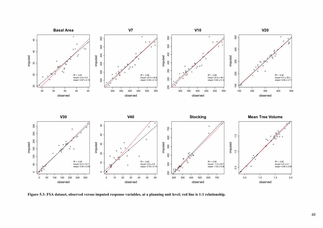
48

Figure 5.3: FSA dataset, observed versus imputed response variables, at a planning unit level; red line is 1:1 relationship.

25 30 35 40 45

2530

3540

45Basal Area

observed

impu

ted

R² = 0.81intcpt= 4.8 ± 5.3slope= 0.87 ± 0.15

300 350 400 450 500 550

300

350

400

450

500

550

V7

observedim

pute

d

R² = 0.89intcpt= 25.5 ± 48.8slope= 0.94 ± 0.12

300 350 400 450 500 550

250

300

350

400

450

500

550

V10

observed

impu

ted

R² = 0.89intcpt= 24.5 ± 48.1slope= 0.94 ± 0.12

100 200 300 400 500

100

200

300

400

500

V20

observed

impu

ted

R² = 0.92intcpt= 6.4 ± 36.3slope= 0.98 ± 0.11

0 50 100 150 200 250 300

050

100

150

200

250

300

V30

observed

impu

ted

R² = 0.93intcpt= 6.5 ± 15.7slope= 0.94 ± 0.09

0 10 20 30 40 50 60

010

2030

4050

V40

observed

impu

ted

R² = 0.80intcpt= 2.8 ± 2.9slope= 0.76 ± 0.14

200 300 400 500 600 700

200

300

400

500

600

700

Stocking

observed

impu

ted

R² = 0.95intcpt= -1.5 ± 30.7slope= 1.03 ± 0.08

0.5 1.0 1.5 2.0

0.5

1.0

1.5

Mean Tree Volume

observed

impu

ted

R² = 0.95intcpt= 0.0 ± 0.1slope= 0.96 ± 0.08

49

Figure 5.4: HVP dataset, observed versus imputed response variables, at a planning unit level; red line is 1:1 relationship.

20 30 40 50 60

25

30

35

40

45

50

55

Basal Area

observed

imp

ute

d

R² = 0.77intcpt= 12.7 ± 5.2slope= 0.66 ± 0.14

100 200 300 400 500 600

20

03

00

40

05

00

60

0

TRV

observedim

pu

ted

R² = 0.94intcpt= 36.8 ± 26.8slope= 0.86 ± 0.08

60 80 100 120 140 160 180

60

80

10

01

20

Roundwood

observed

imp

ute

d

R² = 0.41intcpt= 43.1 ± 23.6slope= 0.54 ± 0.25

0 100 200 300 400 500

01

00

20

03

00

40

0

Saw 20+

observed

imp

ute

d

R² = 0.96intcpt= 7.0 ± 16.5slope= 0.91 ± 0.07

0 50 100 150 200 250 300

05

01

00

15

02

00

25

0

Saw 30+

observed

imp

ute

d

R² = 0.91intcpt= 4.8 ± 13.8slope= 0.94 ± 0.12

0 20 40 60 80

02

04

06

0

Saw 40+

observed

imp

ute

d

R² = 0.76intcpt= 2.4 ± 4.4slope= 0.81 ± 0.18

400 600 800 1000 12004

00

60

08

00

10

00

12

00

Stocking

observed

imp

ute

d

R² = 0.85intcpt= 29.8 ± 126.8slope= 0.99 ± 0.17

0.5 1.0 1.5

0.5

1.0

1.5

Mean Tree Volume

observed

imp

ute

d

R² = 0.96intcpt= 0.0 ± 0.1slope= 0.99 ± 0.08

50

Figure 5.5: FSA, observed vs. imputed diameter distributions by planning unit, representative examples.

10 20 30 40 50 60 70

01

02

03

04

05

060

70

Planning Unit: 3018317

dbh (cm)

Sto

ckin

g (

/ha

)

observed imputed %diffNdq

380 430 13.237.9 35.1 7.2

TRV 543.6 529.3 -2.6Vsaw 478.9 446.5 -6.8Vpulp 539.8 524.8 -2.8BA 44.9 44.0 -2.0mtv 1.43 1.23 -14.0

number of plots: 1

ObservedImputed

10 20 30 40 50 60 70

05

10

1520

25

30

35

Planning Unit: 3018505

dbh (cm)S

tock

ing

(/h

a)

observed imputed %diffNdq

261 228 -12.940.1 40.8 -1.8

TRV 415.5 379.1 -8.8Vsaw 375.1 344.5 -8.1Vpulp 413.0 376.9 -8.7BA 34.4 31.0 -9.9mtv 1.59 1.67 4.5

number of plots: 8

ObservedImputed

10 20 30 40 50 60 70

01

02

03

04

0

Planning Unit: 2038202

dbh (cm)

Sto

ckin

g (/h

a)

observed imputed %diffNdq

288 289 0.538.5 38.1 1.1

TRV 418.3 414.9 -0.8Vsaw 371.8 366.6 -1.4Vpulp 415.4 412.0 -0.8BA 35.2 34.6 -1.7mtv 1.46 1.44 -0.8

number of plots: 14

ObservedImputed

10 20 30 40 50 60 70

02

04

060

80

100

Planning Unit: 2039802

dbh (cm)

Sto

ckin

g (/h

a)

observed imputed %diffNdq

767 761 -0.823.5 23.5 0.1

TRV 289.1 283.1 -2.1Vsaw 117.3 112.1 -4.4Vpulp 280.0 274.2 -2.1BA 36.0 35.6 -1.0mtv 0.38 0.37 -1.7

number of plots: 14

ObservedImputed

51

Figure 5.6: HVP, observed vs. imputed diameter distributions by planning unit, representative examples

10 20 30 40 50 60 70

01

02

03

04

050

Planning Unit: P_3601101201

dbh (cm)

Sto

ckin

g (

/ha

)

observed imputed %diffNdq

915 588 -35.829.8 34.8 -16.7

TRV 665.7 570.5 -14.3Vsaw 424.2 418.4 -1.4Vpulp 181.3 127.7 -29.6BA 59.7 55.7 -6.8mtv 0.94 1.10 16.9

number of plots: 11

ObservedImputed

10 20 30 40 50 60 70

01

02

03

04

05

060

70

Planning Unit: P_3601200101

dbh (cm)S

tock

ing

(/h

a)

observed imputed %diffNdq

550 457 -17.034.0 34.7 -2.3

TRV 479.6 426.5 -11.1Vsaw 387.9 298.0 -23.2Vpulp 52.7 85.0 61.4BA 51.4 44.3 -13.7mtv 0.90 1.04 15.6

number of plots: 2

ObservedImputed

10 20 30 40 50 60 70

05

10

15

20

25

30

Planning Unit: P_3102515801

dbh (cm)

Sto

ckin

g (/h

a)

observed imputed %diffNdq

381 442 15.938.5 38.1 0.8

TRV 499.8 555.7 11.2Vsaw 404.7 433.7 7.2Vpulp 77.7 91.1 17.1BA 43.9 49.4 12.4mtv 1.47 1.52 3.4

number of plots: 10

ObservedImputed

10 20 30 40 50 60 70

05

10

15

20

253

0

Planning Unit: P_3600500301

dbh (cm)

Sto

ckin

g (/h

a)

observed imputed %diffNdq

310 354 14.340.0 38.3 4.4

TRV 350.2 387.0 10.5Vsaw 269.7 293.2 8.7Vpulp 59.4 71.7 20.7BA 37.0 39.8 7.5mtv 1.41 1.32 -6.2

number of plots: 18

ObservedImputed

52

The fact that diameter distributions agree reasonably well suggests that the imputation process is capable of retrieving plots that are truly representative of the forest found at the point of imputation. It must be stressed that these are leave-planning-unit-out results. None of the imputed plots originate from the planning unit in which imputation is carried out. Under operational circumstances plots established in the planning unit will not be excluded from the imputation process. Analysis not reported here shows that this improves imputation results.

5.5 Conclusion Plot imputation models with eight response variables were developed and evaluated for two datasets. A list of 120 candidate predictor variables was proposed and two alternative methods for predictor variable selection were compared for each of three variants of the nearest neighbour technique. Stepwise and Genetic Algorithm variable selection techniques were effective in identifying subsets of variables that produced models with improved predictive performance. Variable selection outcomes were however variable due to the stochastic nature of the selection methods. Numerous repetitions of variable selection runs showed that many combinations of variables generated almost equal scores for the prediction performance metric. It is up to the analyst to carefully compare alternative models and to select the model with the preferred properties. The two models with the best prediction precision scores for the two datasets were selected for further analysis. Detailed evaluation of these models demonstrated strong predictive behaviour for commercially important forest metrics such as saw log volume (V20 and Saw 20+). Predictions were weaker for products that were at the extremes of the sawlog size distribution (sawlog with SED > 40 cm) or that were strongly influenced by stand quality (pulp roundwood). Models predicted diameter distributions fairly closely notwithstanding the fact that models were not deliberately designed to predict diameter distributions. This indicates that the imputation process is truly capable of imputing plots that are representative of the forest found at the point of imputation. Results indicate that relative gains in accuracy were comparable for FSA and HVP datasets even when FSA reference plots would appear to be more suitable for LiDAR based plot imputation (FSA plots were larger, uniform in size plots and more accurately located). The results were achieved with operational field datasets that were not optimised for plot imputation. It is reasonable to assume that predictions could be further improved if reference data were collected in a more optimal way.

53

6 Reference data collection

6.1 Introduction Questions which are central to the imputation process are how many reference plots will be needed and how to select the reference plots. The reference plots typically represent only a small subset of the plots in the area of interest. Over the life of this project a large number of simulations were performed to clarify the efficiency gains which are possible by using LiDAR data for survey design and imputation. The key findings are discussed below together with a flowchart which describes how the survey design process can be implemented in practice. The main sampling schemes are subsequently reviewed and compared and observations are made on the practical issues which were encountered. The issue of sample size is addressed by calculating the precision which is achieved in specific situations and using a range of variables and sample sizes. Examples of R programs are also provided which cover some of the commonly used strategies. The key findings are as follows:-

Throughout the study good efficiencies were identified for survey designs using stratification, systematic sampling and/or balanced sampling. These were in addition to the efficiencies which stem from using imputation (see Figure 6.1).

The best “hands-off” design strategy was balanced sampling, which can be done with a

minimum of statistical expertise. The best “hands-on” design strategies were stratification and systematic sampling. These techniques are quite flexible but require some experience to implement correctly.

In the uniform P. radiata plantations of SA, simulations suggest that while imputation

produced good gains in efficiency, additional gains through survey design were more difficult to achieve. Systematic sampling was generally the best option. In the variable stands of Nundle SF, pronounced efficiency gains were observed when using the balanced sampling strategy.

So-called “space-filling” samples also produced very high efficiency gains with the NSW

data. However a cautionary note here is that these samples need to be combined with imputation – if space-filling samples are used with a design-based estimator then the estimates are extremely unreliable.

A number of recent papers have extended the concept of balanced sampling to include

samples which have good auxiliary coverage in addition to being balanced. In terms of efficiency these new methods may eventually surpass all the methods which have been examined so far.

Many of the sampling strategies depend on having LiDAR data available at the time that the

survey is designed. Exceptions include stratification based on management variables, grid sampling and random sampling. If LiDAR data are not available for survey design then the best sampling method is likely to be stratification based on management variables combined with grid sampling within strata (this assumes that the strata are defined by amalgamations of contiguous plots).

Efficiency gains from survey design (and imputation) depend on accurate plot location. Plot

location becomes more accurate when the handheld GPS device has been in position for a period of time (eg 30 minutes) and the GPS data is averaged. Accurate location of plot centres

54

is not an issue for companies who have the means to exactly locate reference plots using differential GPS units. Positional accuracies are also significantly improved by accessing both GPS and GLONASS satellite systems. The implication of this, however, is that efficiency gains from imputation are more likely to be achieved than efficiency gains from survey design.

The sampling process is pivotal in the sense that it will probably be a once-only operation

which will inform a variety of prediction models over subsequent time periods. The prediction process, however, has much more flexibility and hence decisions regarding which, and how many, variables to use in the prediction models could be altered after the actual survey design without seriously compromising the design itself. There would also be the opportunity to revisit and update estimates when new prediction methods become available.

Figure 6.1: Example of efficiency gains which can be achieved using a combination of sampling strategy and imputation

0 50 100 150

02

46

81

0

Sample size

RM

SE

(%

)

RMSE for v7

SRS using averageBalanced sampling using imputation

Method

55

Sampling Flowchart The sampling scheme can be represented by a flowchart (Figure 6.2) which illustrates the how the key inputs are used to determine a set of reference plots.

LiDAR point cloud

Imputation methodEuclidean, RF, k

Key variableV7, V40, BA

Sampling methodbalanced, systematic,

gridSample size

Calculateplot metrics

Specify imputation method

Specify key variable

Determine best variable subsetfor imputation

Specify sampling methodSpecify sample size

Determine design

variables

Selectreference

plots

Population frame

Imputation variables

Designvariables

Referenceplots

Target plots

Figure 6.2: Sampling flowchart Flowchart description Calculate plot metrics – calculate LiDAR variables for each cell/pixel. Determine best variable subset – after specifying key variable/s, imputation method, sample size and domain of interest use a combination of Monte Carlo search and genetic algorithms to find variable subset which provides acceptable precision in terms of the RMSE Determine design variables – based on the proposed sampling method and sample size, the design variables may be a combination of spatial co-ordinates (grid sampling), spatial co-ordinates +

56

imputation variables (balanced sampling) or a subset of imputation variables (systematic sampling). For systematic sampling the number of design variables will depend on the sample size. Select reference plots – based on the sampling method, sample size and design variables the plot sample uses, an appropriate sampling procedure (eg samplecube) is applied to determine the reference plots LiDAR point cloud – database provided by LiDAR contractor with LiDAR variables and spatial information Population frame – complete list of plots (also called cells or pixels) in the domain of interest together with spatial co-ordinates and LiDAR metrics for each plot Key variables - variables to be estimated, for example V7, total stand volume Imputation method – procedure to be used for plot imputation for example, Euclidean nearest neighbour, random forest, number of neighbours (k) Domain of interest – level for which estimates will be produced, for example whole estate, planning unit, compartment Imputation variables – list of auxiliary variables to be used for imputation of target plots Sample size – number of reference plots required to meet PLE constraints Sampling method – preferred method for plot selection, one (or more) of balanced sampling, systematic sampling, grid sampling, stratified sampling or random sampling Design variables – list of auxiliary variables to be used for plot selection Reference plots – list of plots selected by sampling procedure which will be measured using ground-based surveys Target plots – list of all plots in the population frame which are not reference plots

57

6.2 Sample selection methods The simulations demonstrate that efficiency gains from good survey design are achievable and numerous examples have been documented. However as with most sampling situations the optimal design strategy is unique to each situation and depends on a large number of variables including sample size, plot variability, population size, survey aims and the correlation between forestry measures and auxiliary data. Therefore the focus here is on broad outlines – there will be an ongoing need for further investigation and tailoring of survey design to specific situations. Space filling samples These samples aim to have the reference plots located in p-dimensional space (p is the number of design variables) so that the plots are well spaced in terms of an appropriate distance metric. The simulations showed that these samples were quite efficient when used with imputation and very unstable when combined with a design-based estimation strategy. The reason for this is related to the way these samples tend to select plots with unusually large or small values in the covariate space. Some of these may be atypical (for example a plot which is mostly devoid of trees) however the same plot is assigned to all or most of the samples in a typical simulation. It is noted that (Junttila et al., 2013) made use of space filling samples in a recent paper although they used regression models rather than design-based methods. These samples would not be suited to a multi-purpose strategy. While the imputation results would still be quite acceptable, if the same sample was used with a conventional estimator the results would be considerably worse than with any other type of sample. Grid samples Grid samples can be viewed as a special case of space filling samples (in two dimensions) where only x-y coordinates are used. The intention is to produce a sample with maximal separation between the reference plots; the primary difference to grid samples is that the lattice defined by the plot centres is not exactly rectangular. In the simulation studies grid samples were actually defined by placing a rectangular grid across the forest and rejecting plots which lay outside the forest canopy. This can be tricky in practice because the number of plots inside the forest canopy varies according to the grid placement. For example, if only 50% of the total area is actual forest then the initial sample needs to be twice the intended sample because half the plots, on average, will be rejected. It proved easier in practice to choose an even larger initial sample (say 2.2 times intended sample) and then remove any surplus plots at random to achieve the exact sample size. This is probably more of an issue in research simulations where it is important to maintain the intended sample size. In practice a few extra plots may not present any problems. As with space filling samples, the grid samples proved to be somewhat unreliable in terms of efficiency, often worse than random samples. This was especially the case with large samples – the results with small samples were generally satisfactory. When used with design-based estimates the results were generally similar to or better than random samples. The precise reasons for this behaviour are still to be determined and to study this further involves looking at the design-based properties of the sample, in particular the selection probabilities, in some detail. We know that in a rectangular region grid samples and random samples are similar in terms of the plot selection probabilities. However, real forests are amalgamations of unspecified shapes which result from irregular internal and external boundaries. This appears to have an adverse affect on the final estimates. The best suggestion at this stage would be avoid grid samples unless they are combined with another sampling strategy, such as stratification, which allows better control over the sample. This latter design would result in a grid arrangement within conventional strata such as planning units or age classes and would be similar to current survey design practice.

58

Balanced samples Balanced sampling represents the most “hands-off” strategy apart from simple random sampling. Once the design variables and sample size have been determined, the “samplecube” algorithm finds an appropriate sample without further inputs from the user. However, it should be noted that there are “degrees” of balance so that it would be possible to run the sampling program a number of times and choose the sample with the best balance. A balanced sample is formally defined as a sample where the Horvitz-Thomson estimates of the design variables are equal (or nearly equal) to the population values. Horvitz-Thompson is a widely used design-based estimation method where the sampled plots are weighted by their selection probabilities. For example if a reference plot has a 1 in 10 chance of selection then it receives a weight of 10 in the final estimate. The idea of forcing the sample estimates to be equal to the known population values eliminates samples which are atypical in terms of the design variables. By doing this it is hoped that the resulting sample will have minimal variability in terms of the variable of interest. Although balanced sampling is a design-based strategy it also works very well for model-based estimates and it was found during this study to work very well when used with imputation. Balanced samples are relatively new in the statistical literature and there is much still to be learned. For example balanced samples could be designed to cater for specific situations such as small area estimation. Also it might be possible to reconfigure the sample algorithm so that it recognises certain plots as “fixed” (pre-selected by the user) and constructs a sample which is balanced given these or other constraints. The option of having fixed or pre-selected plots is likely to become more important when the sample is optimised to measure changes over time, as may occur with growth modelling. Balanced samples also appear to be robust with respect to the choice of design variables. In Figure 6.3 the survey design was balanced using variables which were considered optimal for imputing the timber variables V7, V30 and STB (stocking). The sampled plots were then used to predict V7. There was very little difference in precision in the final estimates which suggest that a sample which is balanced with respect to one set of LiDAR variables is also balanced with respect to another set. This is a reasonable expectation since most of the LiDAR variables are correlated to each other. Balanced sampling often produced gains in efficiency which were additional to those obtained through imputation. For example, in the SA inventory plots balanced sampling proved to be better than either simple random sampling or stratification (see Figure 6.4). However we note these plots represent a population which has already been stratified according to current practice so that the correct interpretation would be that stratification + balanced sampling was more efficient than say stratification + random sampling.

59

Figure 6.3: Robustness of imputation estimates with respect to the balancing variables

Figure 6.4: Effect of sampling method on imputation estimates in the SA inventory plots.

0 50 100 150

12

34

56

Sample size

RM

SE

Planning unit RMSE for v7 - balanced sampling

v7v30stb

Design variable

0 50 100 150

02

46

Sample size

RM

SE

(%

)

RMSE for v7 - euclidean imputation

SRSStratifiedBalanced

Sampling method

60

Based on the simulation results, balanced samples usually provide good estimates at the estate level. They may not produce the best estimates in specific areas of interest which are smaller than the estate, for example a particular planning unit. This is because the balanced sample algorithm aims to balance the sample across the whole estate and is not designed to achieve balance at any other level. It may be possible to modify the algorithm to make balanced sampling more flexible and this is still being investigated. Although balanced samples don’t always lead to the best possible RMSE no instances were seen where they produce poor samples or completely fail (such as occurs when space filling samples are used with design-based estimators). They represent the best option in terms of providing a reliable sample with minimal user intervention however it is important to monitor the design errors in areas of interest which are deemed critical to the survey. Systematic samples Systematic sampling is a very flexible strategy and there are many alternatives when it comes to survey design. It is useful to consider some specific examples using the LiDAR variables occupied volume (OV), canopy cover (CC) and height. If there were only 30 plots in the sample then the options are very limited and probably the best sample comes from sorting the population frame by the variable best correlated with the measured variable, for example stand volume. In the NSW data this variable would be OV, therefore the final sample would be 30 plots selected sequentially from the population ordered by OV, and using a random start position. If there are 300 plots in the sample then it possible to use more design variables. However because all the design variables are continuous then at least two of them need to be grouped for example OV and CC. If we group both of these into deciles then we can construct a two-way table with 100 cells and 3 plots per cell, on average. Note that some of the cells may be empty and some may have a lot more than 3 plots. When the population frame is sorted by height within CC group within OV group then a systematic sample can be taken, as before, using a random start position. Another option is to group the first design variable (for example OV) into percentiles, which would give 3 plots per percentile group. A systematic sample can then be obtained by sorting the population frame by CC within OV group. A complication which was noticed early on is that the best sorting strategy is not obvious a priori. For example, yet another option which could be more efficient in practice is sorting the population frame by OV within CC group within height group. For these reasons the systematic sampling option requires some user intervention. The best strategy requires preliminary investigation once the LiDAR data are available and needs to be based on a “surrogate” variable. Since stand volume is not a LiDAR variable the surrogate variable needs to be a correlated variable such as OV, mqh (see Table 5.4) or a linear combination of correlated variables. Given enough experience these issues should be resolved and the best strategy for systematic sampling in a given situation would be established. Note that there is a close relationship between systematic and stratified samples. In the above example, once the data have been grouped according to the first two design variables then we have essentially defined 100 separate strata. If the third design variable was actually a random number then the systematic sample based on ordering the population by random variable within CC group within OV group is equivalent to a stratified random sample (with proportional allocation). Stratified samples When it comes to stratification there is a large number of strategies which can be employed. As mentioned above, systematic sampling may be viewed as akin to stratification, therefore one would expect the efficiencies from a well-designed stratified sample to be similar to those of a systematic sample. A simple stratification scheme using age class and site quality was simulated with the SA data and the results were generally better than balanced sampling. However as noted below there have recently been further improvements to balanced sampling which have rendered it more efficient than the current method and more efficient than stratification.

61

Stratified samples represent the most “hands-on” approach to survey design and they could be an option for a company with access to a biometrician or someone familiar with sampling. They are also the most flexible type of sample and offer the highest degree of control in terms of designing a sample which satisfies rigid and/or multiple design objectives. In addition to this they probably represent the best option when LiDAR data is not available for survey design and/or the key LiDAR variables are yet to be identified. If stratification is employed it is critical to use the correct allocation (number of plots per strata) otherwise the results can be considerably worse than random sampling. In the absence of detailed a priori information the best allocation strategy is “proportional” i.e. the number of plots per strata in the sample is proportional to the number of plots per strata in the population. In spite of the flexibility and the widespread use of stratification it is unlikely that this method can make the best use of the large number of auxiliary variables available with LiDAR. A quote from (Grafström and Schelin, 2014) explains the situation:- With only a few qualitative variables, it is possible to use stratification to make sure that the sample’s proportions match the distribution in the population, such as selecting a sample with 50 per cent female and 50 per cent male subjects if that is the distribution in the population. With more variables, stratification soon becomes a too rough method, resulting in too many and too small strata. Moreover, a multivariate stratification becomes somewhat arbitrary. Hence, our proposal is to use instead a sampling design that guarantees that the sample is well spread in the auxiliary space, that is, a design for selecting spatially balanced samples. Recent advances In the last two years a number of papers have appeared which extend the ideas of balanced sampling. For example (Grafström and Lundström, 2013) have argued that samples which are well separated in auxiliary space are also approximately balanced (however the converse is not true). In an extension of this concept (Grafström and Tillé, 2013) introduced the idea of “doubly balanced” samples whereby the sample is designed to be spatially separate (in two or more dimensions) as well as being balanced across separate auxiliary variables. In a comparison using simulated forestry plots (Grafström et al., 2014) found that these types of samples were more efficient than random samples and obtained further efficiencies using unequal probability sampling. However while unequal probability sampling provides better estimates across the whole estate, for example in terms of total volume, it will tend to select the older/taller plots which means that younger planning units may be disadvantaged. It is clear that more work needs to be done in this area and it is also clear that these recent trends are away from conventional designs, for example using stratification and/or grid sampling , and towards designs which make broader use of the auxiliary data. Referring to grid samples Grafström et al. (2014) make the following comment:- A sample well spread in the auxiliary space is more representative (Grafström and Schelin, 2014) than a simple random sample or a sample that is ``only" well spread geographically, e.g., a systematic sample on a grid. Of interest is that (Grafström and Schelin, 2014) provided a distance metric which includes factor variables. This opens the way for inclusion of variables such as slope, aspect or site quality into the list of auxiliary variables used for survey design. We consider below some sampling comparisons which include the recent methods. Table 6.1 contains simulations based on part of the SA data (~3400 contiguous plots). The number of reference plots was chosen to be either 100 or 300 and relative RMSE values were calculated across the whole population as well as for two specific planning units one of which contains 884 plots (28 years old) and the other of which contains 125 plots (30 years old). The imputation method is Euclidean with k=1 and the table is based on 1000 realisations of each sampling scheme.

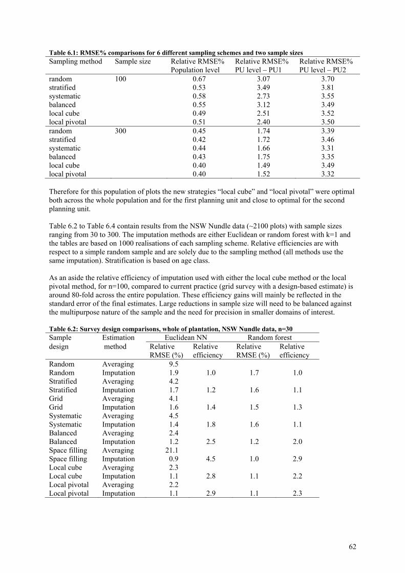
62

Table 6.1: RMSE% comparisons for 6 different sampling schemes and two sample sizes Sampling method

Sample size

Relative RMSE% Population level

Relative RMSE% PU level – PU1

Relative RMSE% PU level – PU2

random 100 0.67 3.07 3.70 stratified 0.53 3.49 3.81 systematic 0.58 2.73 3.55 balanced 0.55 3.12 3.49 local cube 0.49 2.51 3.52 local pivotal 0.51 2.40 3.50 random 300 0.45 1.74 3.39 stratified 0.42 1.72 3.46 systematic 0.44 1.66 3.31 balanced 0.43 1.75 3.35 local cube 0.40 1.49 3.49 local pivotal 0.40 1.52 3.32 Therefore for this population of plots the new strategies “local cube” and “local pivotal” were optimal both across the whole population and for the first planning unit and close to optimal for the second planning unit. Table 6.2 to Table 6.4 contain results from the NSW Nundle data (~2100 plots) with sample sizes ranging from 30 to 300. The imputation methods are either Euclidean or random forest with k=1 and the tables are based on 1000 realisations of each sampling scheme. Relative efficiencies are with respect to a simple random sample and are solely due to the sampling method (all methods use the same imputation). Stratification is based on age class. As an aside the relative efficiency of imputation used with either the local cube method or the local pivotal method, for n=100, compared to current practice (grid survey with a design-based estimate) is around 80-fold across the entire population. These efficiency gains will mainly be reflected in the standard error of the final estimates. Large reductions in sample size will need to be balanced against the multipurpose nature of the sample and the need for precision in smaller domains of interest. Table 6.2: Survey design comparisons, whole of plantation, NSW Nundle data, n=30 Sample Estimation Euclidean NN Random forest design method Relative

RMSE (%) Relative efficiency

Relative RMSE (%)

Relative efficiency

Random Averaging 9.5 Random Imputation 1.9 1.0 1.7 1.0 Stratified Averaging 4.2 Stratified Imputation 1.7 1.2 1.6 1.1 Grid Averaging 4.1 Grid Imputation 1.6 1.4 1.5 1.3 Systematic Averaging 4.5 Systematic Imputation 1.4 1.8 1.6 1.1 Balanced Averaging 2.4 Balanced Imputation 1.2 2.5 1.2 2.0 Space filling Averaging 21.1 Space filling Imputation 0.9 4.5 1.0 2.9 Local cube Averaging 2.3 Local cube Imputation 1.1 2.8 1.1 2.2 Local pivotal Averaging 2.2 Local pivotal Imputation 1.1 2.9 1.1 2.3

63

Table 6.3: Survey design comparisons, whole of plantation, NSW Nundle data, n=100 Sample Estimation Euclidean NN Random forest design method Relative

RMSE (%) Relative efficiency

Relative RMSE (%)

Relative efficiency

Random Averaging 5.17 Random Imputation 0.64 1.0 0.65 1.0 Stratified Averaging 2.31 Stratified Imputation 0.63 1.0 0.62 1.1 Grid Averaging 3.94 Grid Imputation 0.53 1.5 0.62 1.1 Systematic Averaging 3.03 Systematic Imputation 0.54 1.4 0.53 1.5 Balanced Averaging 0.57 Balanced Imputation 0.54 1.4 0.52 1.6 Space filling Averaging 15.79 Space filling Imputation 0.28 5.2 0.52 1.6 Local cube Averaging 0.84 Local cube Imputation 0.44 2.1 0.47 1.9 Local pivotal Averaging 0.84 Local pivotal Imputation 0.44 2.1 0.54 1.4 Table 6.4: Survey design comparisons, whole of plantation, NSW Nundle data, n=300 Sample Estimation Euclidean NN Random forest design method Relative

RMSE (%) Relative efficiency

Relative RMSE (%)

Relative efficiency

Random Averaging 3.22 Random Imputation 0.30 1.0 0.21 1.0 Stratified Averaging 1.36 Stratified Imputation 0.29 1.1 0.20 1.1 Grid Averaging 0.94 Grid Imputation 0.27 1.2 0.19 1.1 Systematic Averaging 0.76 Systematic Imputation 0.25 1.4 0.21 1.0 Balanced Averaging 0.21 Balanced Imputation 0.27 1.2 0.18 1.6 Space filling Averaging 18.92 Space filling Imputation 0.22 1.9 0.14 1.6 Local cube Averaging 0.34 Local cube Imputation 0.23 1.7 0.18 1.9 Local pivotal Averaging 0.36 Local pivotal Imputation 0.24 1.6 0.18 1.4 The relative efficiencies of the various sampling schemes are graphed below for the Euclidean imputation method. Relative efficiencies are more apparent with small sample sizes. As the number of reference plots is increased the less efficient sampling schemes are partly able to compensate. The highest efficiency occurs with the space-filling sampling although this method is not recommended as outlined above. However it does suggest that further efficiencies could be realised in the future.

64

LCM = local cube method LPM = local pivotal method Figure 6.4: Effect of sampling method on relative efficiency in the Nundle plots.  

Determining the best survey design With such a large number of survey designs to choose from a method is needed to compare the various options in a systematic manner. Figure 6.5 illustrates a simple program which calculates a precision value (RMSE) based on a specified survey design on a population of interest. The survey design is repeated a large number of times (B) which would typically be somewhere between 1,000 and 10,000.

50 100 150 200 250 300

01

23

45

Sample size

Re

lata

ive

Effi

cie

ncy

SRS

Stratified

Grid

Systematic

Balanced

LCM

LPM

SpaceFill

Efficiency of various sampling schemes, Nundle plots

65

Figure 6.5: Process for comparing alternative designs and sample sizes

Select reference

plots

Impute values for

target plots

Calculate estimate for AOI

CalculateRMSE

Repeat B times

Sampling method

Sample size

Surrogate variable

Population

B estimates

66

Table 6.2 to Table 6.4 above were based on this type of approach. As mentioned above it is important to monitor the errors in individual planning units especially those which are deemed important to the current survey. The R programs which produced the above table are given at the end of section 6.4 .

6.3 Sample size As with design-based estimates the precision of the imputation estimate improves as the number of reference plots is increased. The best way to appreciate this is to calculate the precision over a range of sample sizes and for different variables of interest. Table 6.5 and Table 6.6 use the SA survey data (304 plots) with sample sizes ranging from 25 plots to 100 plots. Relative RMSE’s are calculated for whole of population estimates (Table 6.5) and also at the plot level (Table 6.6). Probable limits of error are also given at the 5% level of significance. The sampling method used in these tables was random which means that higher levels of precision would be achievable if one of the other sampling schemes was being used. Table 6.5: Sample size vs estate level RMSE%, SA 300-plot data Forestry variable

Sample size Relative RMSE (%)

PLE (%)

V7 25 2.4 4.8 50 1.5 3.0 100 0.9 1.8 V10 25 2.3 4.6 50 1.5 3.0 100 0.9 1.8 V20 25 2.8 5.6 50 1.5 3.0 100 1.0 2.0 V30 25 5.9 11.8 50 4.0 8.0 100 2.2 4.4 V40 25 24.7 49.4 50 17.6 35.2 100 10.7 21.4 MTV 25 2.9 5.8 50 2.0 4.0 100 1.2 2.4 STB 25 3.9 7.8 50 2.3 4.6 100 1.5 3.0 BA 25 2.4 4.8 50 1.4 2.8 100 0.9 1.8 mqh 25 1.8 3.6 50 0.9 1.8 100 0.5 1.0

67

Table 6.6: Sample size vs plot level RMSE%, SA 300-plot data Forestry variable

Sample size Relative RMSE (%)

PLE (%)

V7 25 15.1 30.2 50 13.6 27.2 100 12.4 24.8 V10 25 15.1 30.2 50 13.6 27.2 100 12.4 24.8 V20 25 16.8 33.6 50 15.2 30.4 100 14.1 28.2 V30 25 35.6 71.2 50 33.0 66.0 100 30.8 61.6 V40 25 139.3 278.6 50 132.6 265.2 100 125.7 251.4 MTV 25 17.9 35.9 50 16.7 33.4 100 15.8 31.6 STB 25 21.9 41.8 50 19.2 38.4 100 17.5 35.0 BA 25 14.2 28.4 50 12.8 25.6 100 11.7 23.4 mqh 25 12.0 24.0 50 9.5 19.0 100 7.6 15.2 From these tables we can see that the LiDAR variable mqh is estimated with better precision than the other forestry variables and this is true both across the population and at the plot level. This information is valuable when using mqh as a surrogate variable – we need to take into account that the survey “design” precision, obtained using mqh, will not be achieved for the actual forestry variables. Therefore the number of reference plots will need to be adjusted accordingly. Note the poor precision which typically occurs at the plot level and the also the difficulty in estimating the variable V40 which represents the volume of large timber logs. Table 6.7 uses the SA Green Triangle LiDAR data (33,807 plots) and provides relative RMSE’s for sample sizes ranging from 50 plots to 1000 plots using the surrogate variable mqh. Precision has been calculated across the whole estate as well as in two specific planning units, a large planning unit (PU1 - 1064 plots) and a smaller one (PU2 - 125 plots).

68

Table 6.7: Sample size vs RMSE%, SA 34,000-plot data Forestry variable

Level of estimate

Sample size Relative RMSE (%)

PLE (%)

mqh Estate 50 1.09 2.2 150 0.55 1.1 300 0.44 0.9 500 0.39 0.8 1000 0.31 0.6 PU-1 50 4.58 9.2 150 2.49 5.0 300 1.76 3.6 500 1.37 2.7 1000 1.03 2.1 PU-2 50 4.30 8.6 150 3.55 7.1 300 3.41 6.8 500 3.32 6.6 1000 2.94 5.9 Using this table we would anticipate that the precision (RMSE% across the whole estate) of the surrogate variable mqh is likely to around 1.1% with 50 reference plots and around 0.4% with 500 reference plots. By applying the results from Table 6.5 we would anticipate that the precision (RMSE% across the whole estate) of the timber variable V7 is likely to be around 1.8% with 50 reference plots and around 0.7% with 500 reference plots.

6.4 Conclusion Comprehensive datasets from NSW and SA were used to investigate various issues relating to plot sampling. Good efficiencies were found in a number of sampling methods especially the recent methods related to balanced sampling. These methods are more suited to the large number of auxiliary variables which are associated with LiDAR. More conventional sampling methods such as grid sampling and stratification proved to be less efficient than the newer methods. A flowchart was devised (Figure 6.2) to capture the key steps involved in survey design in the general situation. A second flowchart (Figure 6.5) illustrates the process of determining the most efficient sampling strategy in a specific situation. RMSE values were calculated for a range of sample sizes and forestry variables, including the possible surrogate variable mqh which may be employed in survey design. For large sample sizes (n=1000) the expected RMSE for the surrogate variable was 0.3% across the entire SA estate (~34000 plots) and approximately 2.9% over a small planning unit (~125 plots). For very small sample sizes (n=50) the expected RMSE for the surrogate variable was 1.1% across the entire estate and approximately 4.3% over a small planning unit. RMSE values for the surrogate variable can be calculated for any estate where LiDAR data is available and will assist in selecting an appropriate sample size. It is likely that the more recent sampling methods will eventually become the method of choice with imputation strategies. One issue which is still to be determined is how these methods can be modified to make them more efficient for the purpose of small area estimation. A related issue is that of “conditional” sampling whereby a new set of reference plots is selected to augment an existing set of reference plots which have already been measured or are part of an ongoing survey.

69

Examples of R programs used in sampling Balanced samples require(sampling) # note the use of a dummy variable to ensure the specified sample size is achieved pop.frame$dummy <- 1 # define the imputation variables xvar <- c('height', 'meanht', 'mam', 'mdh', 'pstk', 'var', 'cc') # define the design variables balvar <- c('dummy', 'x', 'y', xvar) # population size N <- 1496 # sample size n <- 50 # select balanced sample ids <- samplecube(as.matrix(pop.frame[,balvar]), rep(n/N,N)) ref.plots <- pop.frame[ids==1,] Spatially balanced samples using recent methods require(BalancedSampling) # define the imputation variables xvar <- c('height', 'meanht', 'mam', 'mdh', 'pstk', 'var', 'cc') # define the design variables balvar <- c( 'x', 'y', xvar) # standardise design variables st_balvar<-scale(pop.frame[,balvar]) # population size N <- 1496 # sample size n <- 50 # selection probabilities pik<- rep(n/N,N)) # select sample using local cube method sid <- lcube(pik,pop.frame[,balvar], cbind(pik)) ids<-rep(1,N)*!is.na(match(1:N,sid)) ref.plots <- pop.frame[ids==1,] # select sample using local pivotal method sid <- lpm(pik,st_balvar, h=N) # h can be reduced with larger datasets to reduce running time ids<-rep(1,N)*!is.na(match(1:N,sid))

70

ref.plots <- pop.frame[ids==1,] Space filling samples This example uses just the x-y coordinates. These aim to maximise the distance between plots, similar to a grid sample, although the lattice points are not rectangular as in a grid sample. require(fields) # population size N <- 1496 # sample size n <- 50 # define coordinate variables cvar <- c('x', 'y') # select space filling sample ids <- cover.design(R=pop.frame[,cvar], nd=n, nruns=10, nn=F, P=-100, Q=100, max.loop=100)$best.id ref.plots <- pop.frame[ids,] Systematic samples require(sampling) # population size N <- 1496 # sample size n <- 50 # define stratification variable/s, if any – in this example only one stratum pop.frame$stratv <- 1 # define quantiles for first design variable (ov) pop.frame$ov5 <- + cut(pop.frame$ov,quantile(pop.frame$ov,seq(0,1,0.05)),include.lowest=T) # note - with 20 quantiles and n=50 there will be approximately 2-3 reference plots # per quantile # sort the population frame by second design variable (height) within quantile pop.frame <- pop.frame[order(pop.frame$ov5, pop.frame$height),] # select systematic sample sid <- strata(pop.frame, 'stratv', size=n, method='systematic', pik=pop.frame$stratv)$ID_unit ref.plots <- pop.frame[sid,]

71

Stratified samples require(sampling) # population size N <- 1496 # stratification variables – in this example planning unit (pu) is used to define strata stratum # calculate stratum sample sizes, overall sample size is 50 ns<-round(50*table(popframe$pu)/N) # select stratified sample sid <- strata(popframe,stratanames= 'pu', size=ns, method='srswor')$ID_unit ref.plots <- pop.frame[sid,] Program to calculate relative RMSE based on repeated sampling require(yaImpute) require(randomForest) # number of plots across estate and in planning units of interest N<-33807;Npu<-1064;Npu2<-125 # surrogate variable yvars<-'mqh' # actual mean act<-mean(tdb[,yvars]) # B is the number of repetitions B<-1000 # code for repeated random sampling # other sampling methods are similar to this dbe<-impe<-impepl<-impepu<-impepu2<-numeric(B) for(i in 1:B){ # random sample sid<-sample(1:N,size=n) ids<-numeric(N);ids[sid]<-1 nid<-is.na(match(1:N,sid)) * c(1:N);nid<-nid[nid>0] # define reference plots and target plots refs<-tdb[sid,];targ<-tdb[nid,] # euclidean nearest neighbour method with k=1 nn<-yai(x=refs[,impvars],y=refs[,yvars],method='euclidean',k=1) # nearest neighbour set for target plots nntarg<-newtargets(nn,targ) # impute Y variables for target plots targ$y<-impute(nntarg,vars=yvars(nntarg))$y # the imputation estimate comes from adding the known values for the reference plots # to the imputed values for the target plots impe[i]<-(sum(refs[,yvars])+sum(targ$y))/N # design-based estimate is just the mean dbe[i]<-mean(refs[,yvars]) # at the plot level the rmse is calculated from the target plots impepl[i]<-100*sqrt(mean((targ[,yvars]-targ$y)^2))/mean(targ[,yvars]) # imutation estimate for pu=3018507 impepu[i]<-(sum(refs[refs$pu=='3018507',yvars])+sum(targ[targ$pu=='3018507','y']))/Npu

72

# imutation estimate for pu=2038304 impepu2[i]<-(sum(refs[refs$pu=='2038304',yvars])+sum(targ[targ$pu=='2038304','y']))/Npu2 } # mean of estimates and true value mean(impe);mean(dbe);act # relative RMSE % across the population 100*sqrt(mean((act-impe)^2))/act # design-based RMSE % #100*sqrt(mean((act-dbe)^2))/act # mean relative RMSE % at plot level mean(impepl) # mean of estimates and true value for pu=3018507 mean(impepu);actpu # relative RMSE % for pu=3018507 100*sqrt(mean((actpu-impepu)^2))/actpu # mean of estimates and true value for pu=2038304 mean(impepu2);actpu2 # relative RMSE % for pu=2038304 100*sqrt(mean((actpu2-impepu2)^2))/actpu2

73

7 Plot imputation across an area of interest

7.1 Introduction Once an imputation model has been developed the model can be applied across an area of interest (AoI). This involves partitioning of the area of interest into tessellating cells, calculation of predictor variables in each of the cells and imputation of the reference plot “nearest” to those predictor variables. The plot imputation process is mostly straightforward but gets more complicated near boundaries separating forest types, land uses, age and management classes. Alternative ways of dealing with such boundaries are proposed. Examples of mapped plot imputation end-products are shown for the South Australian study sites. Aspects of the imputed surfaces are investigated in more detail, in particular the geographic origin, age and site quality of imputed plots relative to the point of imputation. These findings will be discussed in the context of growth modelling and yield table generation which often rely on geography, age and site quality as drivers.

7.2 Processing options Typically spatial partitioning is accomplished by overlaying a square grid across the area of interest. There appears to be general consensus in the literature that grid cells should have an area that is equal or similar to the area of the reference plots used to calibrate the imputation model. The principal reason was mentioned earlier, namely that the values of some LiDAR predictor variables are dependent on the area of the plot in which they have been calculated. Predictor variables need to be calculated within each of the grid cells. This is straightforward and Chapter 8 mentions some of the commercial tools available for this. As with conventional field sampling, complications arise were grid cells straddle different land uses, forest types, tree species, management and age classes. Essentially boundaries can be dealt with in two ways:

1. To mostly ignore them 2. To let the boundaries define distinct assessment units (AU) and then process each AU

individually taking care only to use the LiDAR data inside the AU. To (1): All the LiDAR data falling in the boundary cells are used without any further manipulation. The LiDAR metrics calculated in the boundary cells will be influenced by the mix of forest types, land uses, species, age classes occurring in the cell. If no reference plots with the same mix of forest types, land uses, species, ages are available in the reference database – which is likely - then the imputed plot will poorly represent the real conditions at the point of imputation. The mean imputed value for any arbitrary sub-area can be calculated as the mean of all the cells within that sub-area. Alternatively cells intersecting with the boundary of the sub-area or with centroid outside the sub-area may be excluded from the calculation. This is a practical approach that greatly simplifies data processing at the cost of some fuzziness near boundaries.

74

To (2): This can be a more precise approach as long as the boundaries that define the AU are accurate and accurately co-registered with the LiDAR data. Ideally the LiDAR data themselves would have been used to construct or revise the boundaries. This is in fact a good way to add value to the LiDAR data. The AU need to be processed one by one and LiDAR data need to be clipped to each individual AU. Boundary cells will be cut in two (or more) parts by the boundary. Only one part will be used for imputation. This part will have an area smaller than the standard cell. This will have an impact on some LiDAR metrics. When calculating the mean imputed value for any arbitrary sub-area then the areas of cells need to be used as weights. This approach is clearly more complex and computing intensive. The precision gains will not necessarily be material but mapped end-products may look neater. The operational system described in Chapter 8 adopts approach (1). The examples shown in 7.3.1 adopt approach (2).

7.3 Plot imputation across the South Australian study sites Plot imputation results are shown for the South Australian dataset. The imputed plots are analysed with regard to their geographic origin, age and site quality relative to the point of imputation. Planning unit level yield estimates calculated from the imputed surfaces are compared with yield estimates based on field plots located in the planning units. 7.3.1 Examples of imputed information surfaces The imputation maps shown in Figure 7.1, Figure 7.2 and Figure 7.3 were generated using the random forest model with 6 predictor variables described in 5.4.2. As mentioned in section 7.2 an assessment unit based approach was used to generate these end-products. The planning units in the South Australian estate, also called logging categories, were chosen as assessment units. These are areas consisting of one or more sub-compartments that are uniform in terms of age and harvesting history (the top panel of Figure 7.1 shows the planning units in the study area). They are also designed to have a similar harvesting future. Planning units by design are 100% effectively stocked. The process followed for deriving these end-products is as follows:

Generate a square grid with grid cell area of 0.1 ha large enough to cover the survey area For each planning unit (PU):

o Identify and merge LiDAR tiles overlapping with the PU o Normalise the LiDAR data (normalising is the recalculation of LiDAR heights above

sea level to heights above DEM) o Excise all LiDAR data outside the PU o Overlay the square grid across the PU and calculate LiDAR predictor metrics in each

cell. Delete cells with no LiDAR data in it Retrieve ancillary (non-LiDAR) metrics for each cell (using GIS) Calculate age interaction predictor variables. Using the imputation model and the LiDAR/ancillary predictor metrics impute a reference

plot in each of the cells Load cell data into GIS. The cells are now stored as polygons in a spatial layer, with plot

response variables as attributes. As such they can be submitted to further spatial analysis and mapping.

Apart from the PU-centric processing the process is very similar to that described in Chapter 8. The reader is referred to this chapter for additional detail on tools and software.

75

Figure 7.1: Planning units, imputed volume maps for log to 7cm and 30 cm small-end diameter under-bark (i.e. V7 and V30).

1998

1998

1981

1981

1981

1998

1998

1998

1981

19821981

1981

19981993

1981

1998

1998

1982

1982

1993

1993

1993

1993

1993

1981

1982

1981

1982

1982

1981

1993

1981

1982

1982

1981

1993

1982

1982

1982

1982

1981

1998

1998

1981

1981

1982

1982

19821982

1981

198219821982

1982

1982 19811982 1982

1982

1980

1982

1982

Vol (m3 / ha)

0-50

50-100

100-150

150-200

200-250

250-300

300-350

350-400

400-450

450-500

500-550

550-600

600-750

750+

Planning Units

Grid: Imputed volume to 30cm Small End Diameter. Circles: measured volume

Grid: Imputed volume to 7cm Small End Diameter. Circles: measured volume

76

Figure 7.2: Thinning state, imputed stocking and infra-red photography

1998

1998

1981

1981

1981

1998

1998

1998

1981

19821981

1981

19981993

1981

1998

1998

1982

1982

1993

1993

1993

1993

1993

1981

1982

1981

1982

1982

1981

1993

1981

1982

1982

1981

1993

1982

1982

1982

1982

1981

1998

1998

1981

1981

1982

1982

19821982

1981

198219821982

1982

1982 19811982 1982

1982

1980

1982

1982

Stocking (trees / ha)

150 - 200

201 - 300

301 - 400

401 - 500

501 - 600

601 - 700

701 - 800

801 - 900

901 - 1000

Last Harvesting Operation

Infrared photography - 50 cm resolution

Grid: Imputed stocking. Circles: measured stocking

Last Operation

T1

T2

T3

Clearcut

Ineffective

77

Figure 7.3: Site Quality map and imputed maps of mean tree volume and basal area.

1998

1998

1981

1981

1981

1998

1998

1998

1981

19821981

1981

19981993

1981

1998

1998

1982

1982

1993

1993

1993

1993

1993

1981

1982

1981

1982

1982

1981

1993

1981

1982

1982

1981

1993

1982

1982

1982

1982

1981

1998

1998

1981

1981

1982

1982

19821982

1981

198219821982

1982

1982 19811982 1982

1982

1980

1982

1982

mean tree volume (m3 / ha)

0.25-0.50

0.50-0.75

0.75-1.00

1.00-1.25

1.25-1.50

1.50-1.75

1.75-2.00

2.00-2.25

2.25-2.50

2.50-2.75

Site Quality

Grid: Imputed Basal Area. Circles: measured BA

Grid: Imputed mean tree volume. Circles: measured mean tree volume

Basal Area (m2/ha)

20-25

25-30

30-35

35-40

40-45

45-50

50-55

Site Quality

I

II

III

IV

V

VI

VII

VII-

78

Comments to Figure 7.1 to Figure 7.3:

The three figures show the good agreement between the observed response variables in the field plots and the imputed maps. Note that some PU have field plots while others do not. Reference plots could be imputed in any PU, including in the PU of origin.

The relationships between the various maps make sense: fewer thinning operations produce higher stocking; higher stocking produces lower mean tree volume; high mean tree volume is associated with high V30; it is impossible to have high V30 at young age; basal area maps show the same patterns as Site Quality maps.

The three figures show the significant variability within PU. Is this information of use to operational/harvest planning and logistics? Does it add value over and above the conventional PU level estimates of volumes and products?

7.3.2 Location, age and site quality of imputed plots relative to point of imputation This Section examines the distance between point of imputation and origin of the imputed plot. Similarly it compares the age and site productivity at the point of imputation with those recorded in the imputed plot. This analysis is helpful for two reasons:

To compare imputation behaviour with expectations. For example, does the imputation behaviour agree with Tobler’s First Law (Tobler, 1970), often called the first law of geography: “everything is related to everything else, but near things are more related than distant things”. So if a distant thing is imputed in preference of a near thing is there a plausible explanation?

Age and site productivity index are important input variables in growth models. Biometry is often geographically differentiated. The observed differences between imputed plot and point of imputation have a bearing on how to proceed with growth modelling: should the imputed values of these variables be used or the values observed at the point of imputation? Practical consequences of the answer to this question are significant from a data processing perspective as explained in 8.4.1.

Figure 7.4 shows how the South Australian study area consists of two study sites that are some 40km apart. No restrictions were imposed on where a plot could be imputed, so a plot measured in the Myora forest could be imputed in the Penola forest, and vice versa. Distance from point of imputation to location of imputed plot. The box plots in Figure 7.5 describe the distribution of the distances between points of imputation and location of the imputed reference plots, in sampled and unsampled planning units. A sampled PU is a PU with at least one reference plot in it. The first two characters of the PU code refer to the forest the PU is located in, the middle four digits are the planting year, the final two digits are a sequential number. In the box plots the vertical bold bars represent the median of the observed distances in the PU, the two parts of the box represent the 2nd and 3rd quartile of the data with the length of the box equal to the inter-quartile range. Uneven length quartile ranges indicate skewed distributions. The whiskers extend to 1.5 times the inter quartile range and typically contain more than 95% of the data. Points represent outliers. The top panel of Figure 7.8 provides an alternative representation of these distances.

79

Figure 7.4: The two South Australian study sites Figure 7.5 shows that in 84% of PU the median distance is less than 10,000 m, indicating that in those PU most imputed plots originate from the same forest. For sampled PU the percentage was 94%, for unsampled PU the percentage was 76%. This agrees with expectations. But the figures also show that often some of the plots will be imputed from a different forest, even when the PU is sampled. This will however only occur when comparable (age, harvesting history) PU are present in the other forest. When such plantations are not present there is no cross-forest imputation (for example see PU My-1998-1&2, My-1993-1&6. Figure 7.6 shows the distribution of the differences between the age of imputed plots and the age of the plantation in which they are imputed. The middle panel of Figure 7.8 provides an alternative representation of these differences. The expected value for these age differences is zero, or close to zero. Figure 7.6 shows that in all but one PU the imputed age is within 4 years of the true value 95% of the time (check box whiskers). In a majority of PU the imputed age is within 2 years of the true value 95% of the time. Large median age differences only occur in unsampled PU that are much older/younger than any sampled PU (for example PU My-1971-1. Figure 7.7 shows the distribution of the differences between site quality of the imputed plot and the mapped site quality at the locus of imputation. These differences are expressed in terms of whole Site Quality classes. The bottom panel of Figure 7.8 provides an alternative representation of these differences.

"

!

!

!

!

!

!

!

!

!

!

!

!

Yahl

Glencoe

Wandilo

Mil Lel

Caroline

Tarpeena

Kongorong

Nangwarry

Mt. Schank

Kalangadoo

Mt McIntyre

Mount Gambier

Allendale East

460000

460000

470000

470000

480000

480000

490000

490000

500000

500000

5800

000

5800

000

5810

000

5810

000

5820

000

5820

000

5830

000

5830

000

584

0000

584

0000

10 0 105 Kilometers

Study Sites

Myora Forest

Penola Forest

40 km

80

Figure 7.5: Tukey box plots showing the distribution of distances between reference plot locations and point of imputation, for sampled and unsampled planning units.

Figure 7.6: Tukey box plots showing the distribution of differences in age of imputed plots and plantation age, for sampled and unsampled planning units

My-1981-12

My-1981-2

My-1982-1

My-1982-10

My-1982-2

My-1984-1

My-1984-2

My-1984-7

My-1993-1

My-1993-6

My-1998-1

My-1998-2

Pe-1981-1

Pe-1982-1

Pe-1983-12

Pe-1983-13

Pe-1983-15

Pe-1983-17

Pe-1983-2

Pe-1983-4

Pe-1983-5

Pe-1983-6

Pe-1984-10

Pe-1984-14

Pe-1985-5

Pe-1985-7

Pe-1985-8

Pe-1988-19

Pe-1989-13

Pe-1989-17

Pe-1989-9

Pe-1990-13

Pe-1990-5

0 10000 20000 30000 40000

Sampled Planning Units

Distance to imputed plot (m)

Pla

nn

ing

Un

it

My-1971-1My-1980-10My-1980-11My-1980-12My-1980-13My-1980-19My-1980-4My-1980-5My-1980-6My-1980-7My-1980-8My-1980-9My-1981-1

My-1981-10My-1981-3My-1981-4My-1981-5My-1981-7

My-1982-15My-1982-3My-1982-4My-1982-9My-1983-4

My-1983-44My-1983-45My-1983-46My-1983-6My-1985-1

My-1985-41My-1995-7My-1995-9

My-1998-11Pe-1979-2Pe-1980-1Pe-1980-4

Pe-1983-16Pe-1983-18Pe-1983-7Pe-1983-8

Pe-1984-16Pe-1984-4Pe-1985-4Pe-1992-7Pe-1993-7

0 10000 20000 30000 40000

Unsampled Planning Units

Distance to imputed plot (m)

Pla

nn

ing

Un

it

My-1981-12

My-1981-2

My-1982-1

My-1982-10

My-1982-2

My-1984-1

My-1984-2

My-1984-7

My-1993-1

My-1993-6

My-1998-1

My-1998-2

Pe-1981-1

Pe-1982-1

Pe-1983-12

Pe-1983-13

Pe-1983-15

Pe-1983-17

Pe-1983-2

Pe-1983-4

Pe-1983-5

Pe-1983-6

Pe-1984-10

Pe-1984-14

Pe-1985-5

Pe-1985-7

Pe-1985-8

Pe-1988-19

Pe-1989-13

Pe-1989-17

Pe-1989-9

Pe-1990-13

Pe-1990-5

-5 0 5 10 15

Sampled Planning Units

Age difference with imputed plot (years)

Pla

nn

ing

Un

it

My-1971-1My-1980-10My-1980-11My-1980-12My-1980-13My-1980-19My-1980-4My-1980-5My-1980-6My-1980-7My-1980-8My-1980-9My-1981-1

My-1981-10My-1981-3My-1981-4My-1981-5My-1981-7

My-1982-15My-1982-3My-1982-4My-1982-9My-1983-4

My-1983-44My-1983-45My-1983-46My-1983-6My-1985-1

My-1985-41My-1995-7My-1995-9

My-1998-11Pe-1979-2Pe-1980-1Pe-1980-4

Pe-1983-16Pe-1983-18Pe-1983-7Pe-1983-8

Pe-1984-16Pe-1984-4Pe-1985-4Pe-1992-7Pe-1993-7

-5 0 5 10 15

Unsampled Planning Units

Age difference with imputed plot (years)

Pla

nn

ing

Un

it

81

Figure 7.7: Tukey box plots showing the distribution of differences between imputed plot site quality and mapped Site Quality, for sampled and unsampled planning units Figure 7.7 and Figure 7.8 show the close agreement of imputed and mapped site productivities. The median difference is zero for 100% of sampled PU and 74% of unsampled PU. For most PU (sampled or unsampled) 95% of the differences are no larger than 2 classes.

7.4 Calculating stand parameters for an area of interest The forest parameter maps shown in Figure 7.1, Figure 7.2 and Figure 7.3 can be used to calculate forest parameter means or totals for any area of interest covered by the map. The population total across an area is ∑ with the cell area and the imputed forest parameter, expressed per hectare.

The population mean across an area is ∑

∑.

Means were calculated based on the imputed surfaces for each of the 32 PU and compared to the means based on the reference plots occurring in the PU (see Figure 7.9). As expected the agreement of imputation and sample based population means is as good if not better than in Figure 5.3 because, unlike in Figure 5.3, all available plots contributed to the model and plots could also be imputed in the PU of origin. What is really required now is that the predicted means be compared with realised yield as PU are harvested.

My-1981-12

My-1981-2

My-1982-1

My-1982-10

My-1982-2

My-1984-1

My-1984-2

My-1984-7

My-1993-1

My-1993-6

My-1998-1

My-1998-2

Pe-1981-1

Pe-1982-1

Pe-1983-12

Pe-1983-13

Pe-1983-15

Pe-1983-17

Pe-1983-2

Pe-1983-4

Pe-1983-5

Pe-1983-6

Pe-1984-10

Pe-1984-14

Pe-1985-5

Pe-1985-7

Pe-1985-8

Pe-1988-19

Pe-1989-13

Pe-1989-17

Pe-1989-9

Pe-1990-13

Pe-1990-5

-4 -2 0 2 4

Sampled Planning Units

SQ difference with imputed plot (SQ classes)

Pla

nn

ing

Un

it

My-1971-1My-1980-10My-1980-11My-1980-12My-1980-13My-1980-19My-1980-4My-1980-5My-1980-6My-1980-7My-1980-8My-1980-9My-1981-1

My-1981-10My-1981-3My-1981-4My-1981-5My-1981-7

My-1982-15My-1982-3My-1982-4My-1982-9My-1983-4

My-1983-44My-1983-45My-1983-46My-1983-6My-1985-1

My-1985-41My-1995-7My-1995-9

My-1998-11Pe-1979-2Pe-1980-1Pe-1980-4

Pe-1983-16Pe-1983-18Pe-1983-7Pe-1983-8

Pe-1984-16Pe-1984-4Pe-1985-4Pe-1992-7Pe-1993-7

-4 -2 0 2 4

Unsampled Planning Units

SQ difference with imputed plot (SQ classes)

Pla

nn

ing

Un

it

82

Figure 7.8: Maps illustrating location, age and site quality of imputed plots relative to the point of imputation

Distance to the location where the imputed plot was measured

Difference (classes) between Site Quality of imputed plot and mapped Site Quality at point of imputation.

Difference between age of imputed plot and age at point of imputation

SQ difference (classes)

-4

-3

-2

-1

0

1

2

3

4

Age difference

FieldLasPDHModel

-2

-1

0

1

2

3-5

>5

Distance

nearby (<1000 m)

same forest

different forest

0 250 500 750 1,000125Meters

83

Figure 7.9: Imputed Planning Unit means compared to plot means.

300 350 400 450 500 550

30

03

50

40

04

50

50

0

Vol (to 7cm SED, m3ha

1)

plots

imp

ute

d g

rid

R² = 0.86

100 200 300 400 500

10

02

00

30

04

00

Vol (to 20cm SED, m3ha

1)

plots

imp

ute

d g

rid

R² = 0.92

0 10 20 30 40 50 60

01

02

03

04

05

0

Vol (to 40cm SED, m3ha

1)

plots

imp

ute

d g

rid

R² = 0.92

25 30 35 40 45

30

35

40

Basal Area (m2ha

1)

plots

imp

ute

d g

rid

R² = 0.84

200 300 400 500 600 700

30

04

00

50

06

00

70

0

Stocking (ha1

)

plots

imp

ute

d g

rid

R² = 0.98

0.5 1.0 1.5 2.0

0.5

1.0

1.5

Mean Tree Volume (m3)

plots

imp

ute

d g

rid

R² = 0.97

84

7.5 Growth modelling options The great strength of the plot imputation approach is that whole plots are imputed and those plots can be grown onwards using existing growth models. A yield table for a plot is determined by:

Current state (tree list as measured in the plot) Age (age is a principal driver in even-aged growth models) Site productivity (site quality, site index as predictor of growth) Any geographic variations in biometry (i.e. climate related) Silvicultural history (genetics, fertiliser, thinnings) Future silvicultural regime (thinning, fertiliser)

The tree-list at time of plot measurement provides the starting point for yield table generation. The future silvicultural regime to apply in the plot depends on the regimes applied or management decisions made for the plantation in which the plot was imputed. It seems clear that the future silvicultural regime should not be inherited from the imputed plot. What is less clear is whether imputed plots should inherit their growth predictors (age, site productivity, location) and silvicultural history from the imputed plot or should those observed at the point of imputation be applied? In other words: do we use all the information available for the imputed plot for growth modelling, including site, stand variables and silvicultural history, or do we merely use its tree-list, i.e. the current state? Both approaches have strengths and weaknesses: 1. Inheriting growth predictors from the plot:

Computational efficiency: because age, site index and location are fixed the number of yield tables that will have to be generated for the plot is equal to the number of different harvesting regimes the plot will be submitted to in any of the places where it is imputed.

Growth prediction accuracy: the differences in age, site index and location dependent biometry between plot and point of imputation will introduce errors in growth prediction. The errors will be proportional to the significance of the differences. Note however that the precision of the predictor needs to be considered in this. For example, how precise is the site productivity information at the point of imputation. How precise is the age information at the point of information: what if the point of imputation straddles two age classes?

2. Using the growth predictors at the point of imputation

Computational efficiency: the number of yield tables that will need to be generated for a plot is equal to the number of different combinations of age, site productivity, biometry, silvicultural history (where relevant) and harvesting regime the plot will “experience” at each of its points of imputation. This number will depend on the range of ages, site productivities and geographic range the plot gets imputed to.

Growth prediction accuracy: growth prediction errors may be reduced by using growth predictors specific to the point of imputation, provided these growth predictors are sufficiently precise. The longer the required length of growth prediction the more worthwhile it may be to choose this option. To increase the precision of growth predictors, in particular age, it is preferable to avoid boundary pixels with mixed age. This can be accomplished by using the assessment unit approach described in 7.2.

85

The first approach may be preferable under circumstances where planning horizons are short, where the (spatial) precision of growth predictors is poor or growth models do not require them, survey areas are very large, computing resources are limiting or many alternative cutting strategies need to be tested. The second approach may be preferable under circumstances where planning horizons are longer, where site specific growth predictors are available or where past silviculture has a significant impact on growth prediction. It will require an assessment unit specific imputation approach, as described in 7.2, where assessment units are uniform in terms of the growth predictors. The operational prototype described in the next chapter has adopted the first approach, and describes in more detail why this approach was adopted. A workflow that adopts the second approach may require a different sequence of sub-processes but the sub-processes will essentially be the same.

86

8 Data processing flows of an operational prototype

8.1 Introduction The purpose of this Chapter is to describe the dataflow process of getting from the reference plot data and the LiDAR point cloud to product yield estimates for an area of interest, using plot imputation. The latter half of this Chapter presents the programming structure and data processing subcomponents for the implementation of a plot imputation system Prototype based on LAStools (Isenberg, Rapidlasso) and statistical R software (R-Development-Core-team, 2009). Copies of the actual scripts have been distributed to all the project participants as well as supporting documentation that describes in more detail the usage of each script (“A Plot Imputation System” written by Brian Rawley, Silmetra Limited, NZ). Data-flow diagrams (DFD; http://en.wikipedia.org/wiki/Data_flow_diagram) have been used to illustrate the data flow process because it is often easier to understand a system by the inputs that it requires, the outputs that it produces and the transformations that it performs on the inputs to produce the outputs. Diagram Conventions A data-flow diagram uses only four symbols.

An external entity is a person, organisation or other system outside of the system that provides inputs or receives outputs. A data-flow is a movement of data within the system or across its boundaries. A data-store is a repository for data within the system. A transform is a sub-process that changes inputs into outputs.

8.2 System context Figure 8.1 shows the key output and the key inputs of a plot imputation system. The inputs and outputs are described in following sections. To simplify, the following description assumes a single survey but this does not limit the applicability of the concepts to multiple surveys at different times for different survey areas.

87

Plot Imputation System

LiDAR Provider

Measurement Provider

GIS

User

LiDAR Point Cloud

Reference Plot Measurement 

Data

Reference Plot Location

SurveyBoundary

Area of InterestBoundary

Area of InterestYield 

Estimate

YieldScenario

Non‐LiDAR Metrics

Figure 8.1: Context diagram 8.2.1 Inputs Each of the following sub-sections relates to one of the input data-flows in Figure 8.1 Survey boundary The survey boundary is a boundary of the area within which it makes sense to use plot imputation for the survey. For example, it may not make sense to include lakes within the boundary when the only reference plots are limited to forested areas. Typically the survey boundary will be defined as a polygon or polygons within a GIS system. It will be defined as part of the survey design in the same way that a population boundary or spatial sampling frame would be defined in a conventional inventory. LiDAR point cloud A collection of points in 3D space generated from the returns (reflections) of laser pulses from the ground or forest canopy. At a minimum, each point has an X, Y, Z position in 3D space. Typically a point also has information on its order within the series of returns from a single pulse (e.g. first return).

88

The standard format for storing, exchanging and processing LiDAR point clouds is the LAS file(Sensing, 2013) (.las) or its increasingly prevalent compressed form of the LAS file (.laz) (Isenberg, LASzip: lossless compression of LiDAR data, 2011). The LiDAR point cloud for a reasonable survey area can be huge. Reference plot measurement data This is a sufficient set of data for estimating yields of the products that the survey is targeting for a single reference plot. A typical set of plot measurement data, where the intention is to estimate log products, would consist of:

Reference plot identifier DBH on all trees Heights on enough trees to calculate heights for the un-heighted trees Stem description in situations where it matters Measurement age and/or planted year Other information required by the yield modelling system such as site quality, soil type or

species. Although the focus here is on log products, the plot measurement data can be extended to include other products; for example a plot-level assessment of undergrowth hindrance. For users of YTGen (Yield Table Generator software. Silmetra Limited, NZ) the reference plot measurement data can be thought of as the information in a population file. Plot location The plot location is used to:

associate the plot measurement data with the LiDAR point cloud data when generating LiDAR metrics for the plot

associate the plot with non-LiDAR metrics from other spatial data sets incorporate spatial correlation into the variance estimates of plot yields. For this the plot

centre is adequate information In a typical scenario a plot location will consist of a plot centre along with a known plot radius for a circular plot, or the point locations of plot corners for a rectangular plot. Locational accuracy is important to ensure that the portion of the LiDAR point cloud that is used to calculate LiDAR metrics for the plot is actually consistent with the crowns of the trees that were measured in the plot. For this, a positional accuracy less than a metre is preferred. In practical terms, differentially corrected GPS is a pre-requisite. Survey boundary The boundary of the survey area, typically a polygon or polygons in a GIS. Non-LiDAR metrics Non-LiDAR metrics, like LiDAR metrics, are available for both target pixels and reference plots and are used to determine which reference plot or plots are most similar to each target pixel. Unlike LiDAR metrics, they aren’t generated from the LiDAR point cloud. Examples include the crop age and the reference plot location. In the process of deciding which reference plots are most similar to a target pixel, all things being equal in LiDAR terms, it may be desirable to use reference plots of a similar age in a similar location. Other examples of non-LiDAR metrics include crop or management information, which may be useful predictors of log grades that

89

are not well correlated with LiDAR metrics. Examples in this context include pruned status and crop species. Other potential nonLiDAR metrics could also include local topographic or edaphic attributes such as aspect and slope. Non-LiDAR metrics are typically associated with existing polygons in a GIS. Area of interest boundary The boundary of an area of interest; typically represented by a polygon or polygons in a GIS. Yield scenario The term “yield-scenario” is used here as a catch-all for all of the inputs to a yield modelling system that make for different sets of product yield estimates from a given reference plot. It encompasses things like:

The harvest age The cutting strategy (product specifications) Specifications for thinning events between measurement and harvest

In the YTGen yield modelling system, the equivalent term is a “yield request”. 8.2.2 Outputs Area of Interest Yield Estimate The primary purpose of a plot imputation system is to calculate quantities of products for areas of interest at point in time. Area of Interest Identifier e.g. stand number (where) Point in time e.g. 2015 (when) Product . e.g. Large sawlogs (what) Quantity e.g. 100 m3/ha (how much) Time, in this context, is best thought of relative to a fixed datum, i.e. calendar time, rather than in terms of crop age. It is easy enough to convert from calendar time to crop age in the special case where it is meaningful to assign a year of planting to an area of interest. When future yields from target pixels are averaged across an AOI, they are averaged at a fixed point in time, not a fixed age. The term “product” is used here to reflect a primary interest of commercial forest owners. However, in a more general sense, a product is simply something that can be estimated quantitatively from reference plot data. Other examples of “products” include basal area, crop height, under-storey hindrance and crop age.

8.3 Plot Imputation System Overview Figure 8.2 has the same inputs and outputs as Figure 8.1 but omits the external entities and includes internal data flows and transforms. Each of these is described in more detail in the following sections.

90

Figure 8.2: Plot imputation system overview 8.3.1 Internal data flows and data stores Data-stores are shown in Figure 8.2 to emphasise situations where, in a production system, it is highly likely that the data will be stored for re-use. The main motivation for storing intermediate results is because the same results are used in different transforms or to save time the next time that the same data are needed. Prepared LiDAR point cloud A set of .laz files containing points classified as ground returns or canopy returns, that are within and slightly beyond the survey boundary, where the elevation dimension, (the Z in X, Y, Z) is relative to

91

local ground level and the co-ordinate reference system conforms to local standards. The need to go slightly beyond the survey boundary arises from the need to generate a raster that covers the survey area. The ground returns and above-ground returns may be stored in separate files. Target Metrics Raster A raster of target pixels, with their associated LiDAR and non-LiDAR metrics, that covers the entire survey area. Each cell or pixel of the raster consists of a target pixel identifier, X,Y co-ordinates representing the pixel location and the values of one or more LiDAR or non-LiDAR metrics. In a production implementation it would make sense to store the raster in a spatial database using a specialist raster type. The raster of metrics is much smaller than the point cloud data. Reference Plot Metrics LiDAR and/or non-LiDAR metrics calculated within the boundaries of the reference plots. Nearest Neighbour Raster A raster of target pixels, each with the identifier of one or more reference plots, that covers the entire survey area. The data for each pixel in the raster consists of a target pixel identifier, X,Y co-ordinates representing the pixel location, and a list of reference plot identifiers sorted in order of their similarity to the target pixel in terms of the LiDAR and non-LiDAR metrics. A list of reference plots, as opposed to a single reference plot, is needed for imputation techniques that use more than one nearest neighbour; for example k-nearest neighbours with k > 1. If a measure of similarity between target pixel and associated reference plots will be used in the calculation of a weighted average yield for the target pixel then this will need to be stored. In a research system it would be normal to store a list that is as long as the total number of reference plots in the survey because doing so provides the flexibility to test multiple imputation methods. In a production implementation it would make sense to store the raster in a spatial database using a specialist raster type. AOI Nearest Neighbours In the most general case this is a subset of the nearest neighbour raster that is contained within or associated with an area of interest. If it is sufficient to calculate the average or total yield in the area of interest then this dataset might be reduced to a list of the reference plot identifiers that appear as nearest neighbours to the target pixels in the area of interest, each with a count of the number of times that reference plot identifier appears. On the other hand, if an estimate of the variance of the total yield is required then the list of the k-nearest neighbours for each target pixel is required. Reference Plot Yields This is the same data as the primary output of the system but by reference plot instead of AOI. It consists of: Reference plot Identifier e.g. (where) Point in time e.g. 2015 (when) Product e.g. Large sawlogs (what) Quantity e.g. 100 m3/ha (how much)

92

8.3.2 Transforms Prepare LiDAR Point Cloud There are a number of things that may need to be done to raw LiDAR point cloud data before it is useable. These include:

Transformation to the local standard co-ordinate reference system Removal of outliers Separation of ground returns and canopy returns Generation of a digital elevation model (DEM) from the ground returns Normalisation of the canopy returns to the ground-level Cropping to slightly beyond the survey boundary; just enough beyond to allow generation of

a raster that covers the entire survey area with LiDAR data available for each pixel in the raster.

Tiling and indexing for downstream processing efficiency Data compression (.las to .laz)

Some of these transforms will be carried out by the LiDAR supplier. In cases where the LiDAR point density is low it may be more appropriate to use an existing DEM than to develop one from the LiDAR data from the survey. This work would typically be carried out using specialist LiDAR processing tools like LasTools (Isenberg, LAStools: award-winning software for rapid LiDAR processing) or Fusion (Mc Gaughey, 2014). Calculate Target Metrics This includes creating a raster and associating metrics with each pixel in the raster (Figure 8.2 & Figure 8.3). The pixel size should be similar to reference plot size.

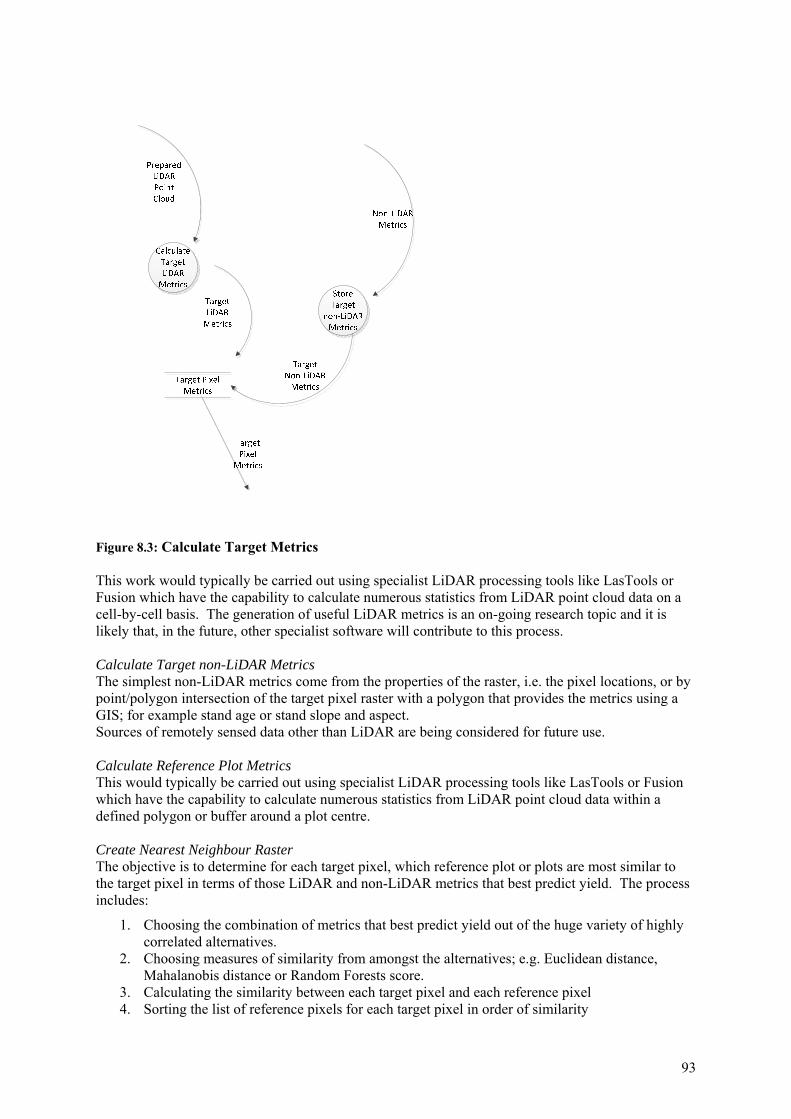
93

Figure 8.3: Calculate Target Metrics This work would typically be carried out using specialist LiDAR processing tools like LasTools or Fusion which have the capability to calculate numerous statistics from LiDAR point cloud data on a cell-by-cell basis. The generation of useful LiDAR metrics is an on-going research topic and it is likely that, in the future, other specialist software will contribute to this process. Calculate Target non-LiDAR Metrics The simplest non-LiDAR metrics come from the properties of the raster, i.e. the pixel locations, or by point/polygon intersection of the target pixel raster with a polygon that provides the metrics using a GIS; for example stand age or stand slope and aspect. Sources of remotely sensed data other than LiDAR are being considered for future use. Calculate Reference Plot Metrics This would typically be carried out using specialist LiDAR processing tools like LasTools or Fusion which have the capability to calculate numerous statistics from LiDAR point cloud data within a defined polygon or buffer around a plot centre. Create Nearest Neighbour Raster The objective is to determine for each target pixel, which reference plot or plots are most similar to the target pixel in terms of those LiDAR and non-LiDAR metrics that best predict yield. The process includes:

1. Choosing the combination of metrics that best predict yield out of the huge variety of highly correlated alternatives.

2. Choosing measures of similarity from amongst the alternatives; e.g. Euclidean distance, Mahalanobis distance or Random Forests score.

3. Calculating the similarity between each target pixel and each reference pixel 4. Sorting the list of reference pixels for each target pixel in order of similarity

94

The last two steps are largely mechanical but the first two include choices and, for the foreseeable future, are likely to require human intervention to decide which metrics and similarity measures are likely to be most satisfactory in a given survey. The yaImpute package in R (Crookston and Finley, 2008) has proven to be a very useful tool for this work. The LiDAR project team have developed R scripts that could provide a starting point for other users. Assign AOI Nearest Neighbours The simplest approach is to take all of the pixels from the nearest neighbour raster where the pixel centre falls within the boundary of the area of interest; a point/polygon or raster/polygon intersection using a GIS. Calculate Reference Plot Yield In a production environment this would typically be handled by generating product yields using specialised software, e.g. YTGen, for each combination of reference plot, yield scenario and future point in time, as a batch process. Results would typically be stored in a data base for re-use. Yields for other yield scenarios could be added as required. One of the simplifying assumptions that makes pre-calculation of yields possible is that the yields for a reference plot are completely independent of the pixels that will ultimately be the targets of imputation; but see “Yields that depend on the target pixel” below for an alternative. Calculate AOI Yield In the simplest case, the average yield for an AOI is simply the average of the yields for each target pixel in the AOI. The yield for a target pixel is the average for the reference plots that are the nearest neighbours to that target pixel, possibly weighted at the target pixel level by a measure of the similarity between target pixel and reference plot metrics. These are simple calculations that can be handled in SQL from a database even when more than one nearest neighbour (k > 1) is used with each target pixel. Calculating the variance of the average, for sampling error (e.g. PLE) calculations, is much more complex. This is because the yield estimates for one target pixel are not independent of the yield estimates for another target pixel. At the very least, two target pixels that share the same reference plot(s) have highly correlated yield estimates. On top of this is an extra layer of complexity if estimates from different reference plots are correlated because the reference plots are close together. Variance estimators for AOIs, using plot-imputation, is still an area of active research but practical model-based methods have been proposed (Mc Roberts et al., 2007) and tested in pilot-scale surveys. Because of the complexity of the calculations, these are best implemented using R scripts.

8.4 Alternatives 8.4.1 Yields that depend on the target pixel There is a view that some attributes of the target pixel should be influential in predicting yield. The easiest example to understand is with reference to crop age. Given a reference plot that was measured at age 20 and becomes the nearest neighbour to a target pixel aged 25 at the time of the survey, the question is: what measurement age should be used to predict the growth of the reference plot for the purposes of estimating future yield; 20 or 25? The data flows in Figure 8.2and the rest of this document use the assumption that the reference plot age will always be used. This has the advantage from a systems point-of-view that:

It reduces the number of yield estimates that must be pre-calculated. When the target pixel is influential then there must be a set of yields for every combination of reference pixel, target pixel age, yield scenario and future point in time. The number of required yield estimates

95

would increase exponentially with the number of yield-determining attributes from the target pixel.

It reduces the likelihood that growth modelling will fail due to serious mismatches between reference pixel age and assumed target pixel age. An example of how this happens is when a target pixel at the edge of a young stand picks up, in its LiDAR metrics, taller trees in a neighbouring older stand and, as a consequence, is matched with an older reference plot. This can result in trying to start a growth model using 30 year old trees from the reference plot with an assumed age of 5 from the target pixel.

Although age is used as an example, “site-quality”, altitude, latitude, soil type, rainfall, species, measurement history and any number of other variables from the target pixel might be used to influence the growth or product qualities of a reference pixel. An alternative to incorporating these attributes in the yield estimation process is to incorporate the important ones in the set of non-LiDAR metrics. This issue will only be resolved through experience. 8.4.2 Target pixel metrics that depend on the crop One weakness with a raster-based approach arises because pixels have a finite size and do not honour crop boundaries. A 30m square target pixel might pick up LiDAR data from two age classes and a fire break. Because of this it might be associated with a reference plot that is, in some way, unlike the crop in which the pixel centre falls. For example, any pixel that is centred on a road that is less than 30m wide will pick up some LiDAR returns from the tree canopy either side of the road and is likely to pick up some yield. This is not a forestry-specific problem; it is just an example of the more general problem of using discrete data (rasters) to represent continuous data when the dimensions of AOIs approach pixel size. One proposed solution to this problem is to clip each target pixel to crop boundaries, so that only LiDAR returns from the crop with which the pixel is associated are used to calculate pixel metrics. As a simple example, a pixel with a centre that falls on road wouldn’t use any canopy returns. This approach maintains independence between the target pixel metrics and the AOI but it does introduce the practical problem of deciding where the crop boundaries are; where the GIS says they are or where the LiDAR data says they are. It also means that if the crop boundaries change then the target pixel rasters must be re-generated. In the context of the system description, use of this approach would imply an extra data flow, in , that represented the dependency of the target pixel metrics on crop boundaries. An alternative proposal is to clip the target pixels to the AOI boundaries. This approach has two additional disadvantages:

The target pixel metrics and nearest neighbours would need to be generated anew for each set of areas of interest. This has computational and storage implications.

The total estimated yield in the forest would become dependent on how the forest was carved up into areas of interest.

In practise, this alternative approach is unlikely to be a serious contender except in situations where there is only one set of AOIs and they are relatively stable.

8.5 A Prototype implementation The following section provides details for software implementation intended to make a basic plot imputation system accessible for learning, experimentation and as a start to incorporating plot imputation into individual systems. It describes the programming structure based on LAStools; R (R-Development-Core-team, 2009) and YTGen software. Copies of the actual scripts that flow from the LiDAR point cloud data through to yield tables have been distributed to all the project participants.

96

HVP Plantations provided the project with the datasets used in this process; consisting of approximately 25,000 ha of LiDAR data, of which 9,500 ha overlapped P. radiata plantation. In addition, they supplied inventory data from 242 plots that covered 940 ha spatially coincident with the LiDAR data. The Prototype software implementation was developed using these data sets to provide a Prototype workflow from LiDAR point cloud data through to:

Product volume estimates, with standard errors, for areas of interest, at or after time of measurement,

Geo-referenced yield surfaces 8.5.1 Software dependencies The LAStools suite of point cloud processing software was used for processing LiDAR data to generate canopy metrics. This dependency only exists to the extent that early stages of data processing by R assume a CSV file in the format generated by LAStools lascanopy. Substitution of alternative software for processing point cloud data would not be difficult. The R programming language is used for the plot imputation and spatial processing. A method is provided for generating reference plot product yields using YTGen; largely because the plot measurement data used in the test case are in that format. However, the structure of yield estimates has been kept as generic as possible so that alternative methods of yield estimation can be readily substituted. This implementation does not depend on a specific GIS or database. Where inputs are spatial, they are provided as ESRI shape files or compressed LAS files. R provides enough spatial processing that a dedicated GIS is not required. There is considerable potential to use a database for storage of input and intermediate data but it was felt that doing so in a prototype would add an extra software dependency and extra complexity that were not required to meet the objectives of the prototype. Intermediate files are stored as R data objects in compressed (.rd) format. Where possible, use is made of existing R classes for storage. These include spatial data types from the sp package (SpatialPixelsDataFrame and SpatialPointsDataFrame) and the yai model class from the yaImpute package. Yield outputs are R data frames stored in compressed (.rd) format which can be exported to CSV format using one of the provided scripts. Yield surfaces are available in GDAL-supported, geo-referenced raster formats (e.g. GeoTiff, XYZ ) for viewing in image viewers or analysis in GIS packages. 8.5.2 User interface No graphical user interface is used in this Prototype. The Prototype implementation is distributed as a set of R scripts. Each script is run from the command-line using the R script executable from the base R distribution. Where a user has choices, these are selected as command-line options, rather than by editing R code. The range of options that are selectable from the command-line has been limited to those that are immediately useful. It is inevitable that user project participants will wish to extend the R code and this is encouraged. Each script has a --help command-line option which prints a short description of what the script does and the command-line options that it supports.

97

Data-flow diagrams are provided to illustrate entire workflow as a series of scripts that flow from LiDAR point cloud data through to yield tables. 8.5.3 Limitations

1. Reference plot yields do not depend on target pixel characteristics. For example, a reference plot that is known to be age 15 at time of measurement will have yields based on the assumption that it is age 15, even when it is selected as nearest neighbour for an age 16 target pixel.

2. Target pixel metrics, nearest neighbours and yields do not depend on AOI boundaries. This has the benefit that, no matter how a yield surface is divided into areas of interest, the total yield will be the same. It has the negative effect of “blurring” of yield at boundaries; for example the boundary between stocked area and roads.

3. It is assumed that spatial inputs will share a common, projected co-ordinate system; e.g. “GDA94 / MGA zone 55” (EPSG:28355). No provision has been made for re-projection of input data. On the other hand, in the interests of documentation, provision has been made to label R spatial objects with an appropriate co-ordinate reference system.

4. No provision is made for converting from a year-indexed yield table to an age-indexed yield table in the output.

8.5.4 Operating environment For Windows users, a 64 bit version of Windows 7 or 8 is recommended. The 64 bit version is recommended because the maximum memory allocated to applications is limited under 32 bit versions to an extent that is likely to pose problems with surveys of a reasonable size. The R scripts were initially developed and tested under a 64 bit version of Linux (Ubuntu 14.04) with 16 Gb of memory. They were subsequently tested under Windows 7 64 bit with 6 Gb of memory. Memory use with the test data is provided in a later section. In both cases, R version 3.1.1 was used. Most of the R scripts will make use of multiple CPU cores if these are available and the parallel package has been installed. Having multiple CPU cores is recommended. Lastools is limited to the Windows environment. 8.5.5 Installation and use R scripts are run from a command environment. Under Windows, the obvious choices are the traditional “DOS prompt” (cmd.exe) or the newer Windows Powershell. The latter is recommended because it has more features that make life in a Windows command-line environment more bearable.

Install lascanopy and lasindex from the LAStools suite and ensure that these are in the search path of the command environment

Install the base R package from http://cran.r-project.org/ . The 64 bit version is recommended because it allows for the processing of larger data sets than the 32 bit version. R 3.1 is recommended for larger data sets.

Install R package dependencies. First -level dependencies from outside the base R installation are:

o optparse for command-line option parsing. o gstat for spatial processing o rgdal for spatial processing o sp for spatial data classes o parallel to use multiple CPU cores to speed up processing. o GA for suggesting predictors using genetic algorithms o lattice for graphics o reshape for reshaping yield tables o yaImpute for building and using neighbour models

98

The parallel and lattice packages should be part of the base distribution. The easiest way to install a local copy of dependencies is to use the install.packages function from inside an interactive R session. This will also install secondary dependencies. e.g. install.packages(c(“optparse”,”gstat”,”sp”,”rgdal”,”GA”,”reshape”,”yaImpute”))

Ensure that Rscript.exe is in the search path of the command environment. The R installer should take care of this.

Install YTGen if this is to be used for generating yields. The installer places the executables in the search path of the Windows command environments.

LAStools, R and the additional R packages install binaries. This may have security implications in your operating environment. These are outside the scope of this report.

8.6 Use of R scripts R scripts are invoked using RScript.exe, which comes with the base R installation. Under Windows, Rscript.exe requires a full or relative path to script file. For example, assuming that the R scripts are in the bin directory under the directory containing project data then the following will work in a Windows envrionment: RScript.exe bin\export_yield_tables.R -v --input=aoi_wide_tables.rd --output=aoi_wide_tables.csv In Unix-like environments, including OS X and Linux, the R scripts, provided that they are in the search path, can be executed directly; e.g. export_yield_tables.R -v --input=aoi_wide_tables.rd --output=aoi_wide_tables.csv

8.7 Data flows Figure 8.4 to Figure 8.8 data flow diagrams show the use of the R scripts in the Prototype work flow. They extend Figure 8.2 to include information on the formats of the data flows and the specific R scripts used in transformations. The data flows start from a position in which the LiDAR point cloud data has been cleaned up, tiled and geo-referenced.

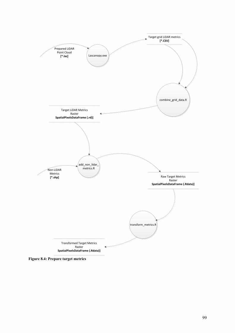
99

add_non_lidar_metrics.R

combine_grid_data.R

Lascanopy.exe

Target grid LiDAR metrics[*.CSV]

Non‐LiDARMetrics[*.shp]

Target LiDAR MetricsRaster

SpatialPixelsDataFrame (.rd)]

Raw Target MetricsRaster

SpatialPixelsDataFrame (.Rdata)]

Prepared LiDAR Point Cloud 

[*.laz]

Transformed Target MetricsRaster

SpatialPixelsDataFrame (.Rdata)]

transform_metrics.R

Figure 8.4: Prepare target metrics

100

Figure 8.5: Prepare Reference Plot Metrics

101

Figure 8.6: Develop imputation model

102

Figure 8.7: Calculate Area of Interest Yields

103

Figure 8.8: Miscellaneous transforms 8.7.1 Inputs

104

Survey boundary A shape file using the project co-ordinate system and containing one or more polygons or multi-polygons defining the survey area. LiDAR point cloud A tiled set of compressed LAS files (.laz) with tile size chosen to facilitate downstream processing, using the project co-ordinate system. Reference plot measurement data A set of YTGen population files, one per plot, with the plot number providing a reference plot identifier that is unique within the survey. Plot boundaries A shape file using the project co-ordinate system, with each polygon defining the boundary for a reference plot. This is identified using the same reference plot identifier in the measurement data. The boundary is used to clip LiDAR point cloud data when calculating reference plot LiDAR metrics. The use of a polygon to define the plot is more general than the use of a centroid and radius and is intended to allow use of non-circular and/or variable size plots. Plot Centres A shape file using the project co-ordinate system, with each point defining the centroid for a reference plot. This is identified using the same reference plot identifier in the measurement data. The plot centre is used to determine which grid cell a plot is associated with and for determining plot-to-plot distances in calculation of spatial correlation. Automatic inference of the plot centre from the boundary has not been provided in the prototype. Non-LiDAR metrics A shape file using the project co-ordinate system and containing a set of polygons. Attached to each polygon are attributes that will be used to generate potential non-lidar metrics for both the target raster and the reference plots. Area of interest boundaries A shape file using the project co-ordinate system and containing one or more non-overlapping polygons or multi-polygons each defining an area of interest. Yield scenario Each scenario is expressed as a YTGen yield request file containing a single yield request specifying cutting strategy, grade recovery rules, user variable rules and thinning events for a single population. Periods, including thinning timing, must be expressed using calendar years. The name of the population is not important. During processing it will be substituted by each of the populations in the reference plot set. A base yield scenario, suitable for variable selection, would consist of a single output period (at time of measurement) and no thinning events. 8.7.2 Internal data stores One of the design imperatives was to break the work flow into small chunks so the each R script, as far as is possible, is responsible for generating a single intermediate or output file. There are several reasons for using this approach:

re-usability of R scripts simplicity reduction of memory use availability of intermediate data sets for examination

105

ability to restart processing at intermediate stages The intermediate data-stores identified in Figure 8.4to Figure 8.8 are described in the following sub sections. Prepared LiDAR point cloud A tiled set of compressed LAS files (.laz) with tile size chosen to facilitate downstream processing and points defined using the project co-ordinate system. Points have been normalised (i.e. point heights expressed relative to local ground-level) and filtered to remove any points that are not useful for calculating canopy metrics. It is highly desirable that tile sets are indexed using lasindex to speed up downstream processing. Target Metrics Raster An R SpatialPixelsDataFrame object stored in compressed Rds format using the R saveRDS function. The SpatialPixelsDataFrame type is provided by the sp library (Pebesma and Bivand, 2005). Raster characteristics, including projection system and cell size are stored with the data. Each row represents a single cell in the target raster, identified by X,Y co-ordinates at the cell centroid using the project co-ordinate system. Other columns represent named LiDAR or non-LiDAR metrics. The raster is sparse, in the sense that cells that are outside the survey boundary, or have missing values, have been removed. This is to save both space and time. Reference Plot Metrics An R data frame stored in compressed Rds format using the R saveRDS function. Each row represents a single reference plot, identified in the row name by reference plot identifier. Other columns represent named LiDAR and non-LiDAR metrics. Nearest Neighbour Raster An R list stored in compressed Rds format using the R saveRDS function. The list contains the following named objects: ids: an R SpatialPixelsDataFrame object. Each row represents a single cell in the target raster, identified by X,Y co-ordinates at the cell centroid using the project co-ordinate system. The other columns, idk1-idkn, contain the reference plot identifiers for the n nearest neighbours to the target cell, ordered in by distance, with idk1 representing the nearest neighbour. The raster is sparse, in the sense that cells that are outside the survey boundary or have no assigned nearest neighbours have been removed. distances: an R SpatialPixelsDataFrame, identical to “ids” but containing the distance to each nearest neighbour. The units and meaning of distance depend on the distance convention of the imputation model. This output is optional and is not used in downstream scripts but is provided for completeness. k.model: an integer storing the value of k (the number of nearest neighbours) in the imputation model that was used to generate the grids. This might be different to the number of nearest neighbours stored in each grid. Reference Plot Yield An R data frame stored in compressed Rds format using the R saveRDS function Each row represents a single reference plot identified in the row name using the reference plot identifier. Each other column represents a single named “yield” variable, for example the basal area or the volume of a specific log grade at a point in time. Each data frame (file) contains a complete set of yields associated with a single yield scenario. Calculation of the average yield for an AOI makes no distinction between different types of yield and it is appropriate in a prototype with a potentially wide range of applications to avoid imposing too much in the way of external structure on the data that will be processed. One example of structure is the view that a yield table is a 2D matrix of product volume by point-in-time. The plot imputation

106

calculations do not need to be exposed to this structure. In the Prototype, any external structure in a set of yields is encoded in the yield names. e.g. Total_trv_CF_2014 or Sawlog_volume_CF_2014. 8.7.3 Transforms (R Scripts) Below is a list of all the R scripts in approximate workflow order. Some R scripts are used in more than one place in the workflow. For example transform_metrics.R is used for both reference plot metrics and target metrics. A more detailed description of each R script is provided in another report “A plot Imputation System” written by Brian Rawley (Silmetra Limited, NZ). This Report, along with the script programming, have been provided to all the project participants.

combine_grid_data.R add_non_lidar_metrics.R combine_reference_plot_data.R transform_metrics.R clip_grid.R compare_metrics.R generate_reference_plot_yields.R suggest_predictors.R create_nearest_neighbour_raster.R calculate_spatial_correlation.R calculate_aoi_yields.R reshape_aoi_yields.R export_yield_tables.R export_yield_surface.R

8.7.4 Outputs Three primary outputs are provided. However, all of the intermediate calculations are available for examination and use. Area of Interest Yield Estimates Without standard errors R data frame with each row representing a single area of interest and each column representing either the average yield for a single yield variable for that AOI. Yield variable name and point-in-time are encoded in the yield variable name. The AOI identifier is in the row name. With Standard Errors R data frame with each row representing a single area of interest and yield variable name with the mean (mu), variance (var) and standard error (se) of the estimate. The number of grid cells in the AOI (n) and the number of distinct reference plots included in the estimate (n.ref) are also included. Area of Interest Yield Table This is a rearrangement of the yield estimate data to provide either:

Long format: one row per AOI, period (point in time), harvest type (thinning or clearfell) and yield variable.

Semi-wide format: one row per AOI, period (point in time) and harvest type (thinning or clearfell) with one column per yield variable.

These can be exported from R data frame to CSV using export_yield_tables.R Yield surfaces Imputed yield rasters are stored internally as a SpatialPixelsDataFrame containing multiple yield variables per file. These can be exported using export_yield_surface.R to supported, GDAL-

107

compliant raster formats, including GeoTiff, with a single yield variable per file. After export they can be viewed and/or analysed using GIS software.

8.8 Scalability Scalability refers to the ability of the Prototype to process large survey areas without failing due to resource limitations. The primary limitations on scalability for this design relate to:

LAS file processing R data processing

Scalability in LAS file processing is handled by tiling of the input data files into manageable sizes and the use of LasTools, which, through spatial indexing, can handle very large survey areas without requiring the whole data be in memory at the same time. R requires that whole data frames are stored in memory for processing. This limits the size of the problem that can be handled using R before the data must be broken down. There are two areas where the size limitation is likely to be felt.

Rasters of target metrics Calculation of estimator variance for AOI yields

8.8.1 Raster size A sparse raster in R (SpatialPixelsDataFrame) uses about 8 bytes of memory for each variable, including the X,Y co-ordinates, for each grid cell. A survey area of 100,000 ha at 10 pixels per ha with X,Y co-ordinates and 30 yield variables or target metrics would take approximately 100,000 x 10 x 32 x 8 bytes or 256 Mb of computer memory for storage or less for disk storage when compression is used. Space in memory for more than one copy of a target grid is required. If the 64 bit version of R is used, this memory usage is not likely to be limiting until survey areas become very large. In the test case, using HVP Plantations data, the only step in the process where memory use was high enough to cause minor consternation was when it was necessary to convert the full rasters generated by LSAtools lascanopy into a single sparse raster. Lascanopy generates results for every cell in every tile. 8.8.2 Variance calculation Calculation of the variance for the average yield of an area of interest requires computation across a co-variance matrix of size N2xk2 where N is the number of cells in the AOI and k is the number of nearest neighbours per cell. For an AOI with 1 million cells, which can happen when the AOI is the whole survey area, and 5 nearest neighbours, the lower triangle of the co-variance matrix has 1.25 x 1013 cells and would take 10,000 Gb of system memory to store. This problem is reduced to manageable size in the prototype implementation by sampling from the co-variance matrix rather than processing it in its entirety as suggested by (Mc Roberts et al., 2007). 8.8.3 Resource use in test case Table 9.1 provides details on processing time and memory use for the Prototype workflow example using the data provided by HVP Plantations. The times were calculated on a PC with an Intel I7-2600K 3.4GHz processor with 4 cores (8 threads). A maximum of 4 cores were allocated to

108

processing. All data was stored on a local hard drive. Memory use is as reported by R for the data used by primary process. This is an under-estimate of total memory use because, in a multi-processor environment, each separate process used copies of some of the data. In the extreme case the total memory use will be the reported value multiplied by the number of cores used. There is a trade-off between processing time and memory use that is, to some extent, under the control of the user. Combining grid data from CSV files used the most memory. This memory use could be reduced significantly by removing empty grid cells from the CSV files in a separate step. The processing bottle-neck is in suggest_predictors.R. This requires the development of multiple imputation models using yaImpute. Using the randomForests yai method in suggest_predictors.R significantly increases elapsed time beyond what is shown in Table 8.1. Each pass through the genetic algorithm using randomForests takes roughly 2 hours. Using 4 CPU cores to generate 100 potential models using the genetic algorithm and randomForests would take approximately 2 days.

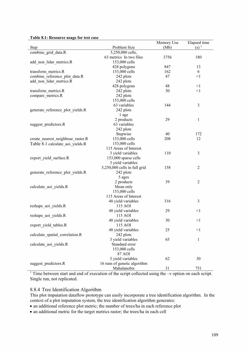
109

Table 8.1: Resource usage for test case Step

Problem Size

Memory Use (Mb)

Elapsed time (s) 1

combine_grid_data.R 5,250,000 cells, 63 metrics In two files 3756 180

add_non_lidar_metrics.R 153,000 cells 428 polygons 847 13

transform_metrics.R 153,000 cells 162 6 combine_reference_plot_data.R 242 plots 47 <1 add_non_lidar_metrics.R 242 plots

428 polygons 48 <1 transform_metrics.R 242 plots 30 <1 compare_metrics.R 242 plots

153,000 cells 63 variables 144 3

generate_reference_plot_yields.R 242 plots 1 age

2 products 29 1 suggest_predictors.R 63 variables

242 plots Stepwise 40 172

create_nearest_neighbour_raster.R 153,000 cells 208 12 Table 8.1 calculate_aoi_yields.R 153,000 cells

115 Areas of Interest 3 yield variables 110 3

export_yield_surface.R 153,000 sparse cells 3 yield variables

5,250,000 cells in full grid 158 2 generate_reference_plot_yields.R 242 plots

5 ages 2 products 39 2

calculate_aoi_yields.R Mean only 153,000 cells

115 Areas of Interest 48 yield variables 316 3

reshape_aoi_yields.R 115 AOI 48 yield variables 29 <1

reshape_aoi_yields.R 115 AOI 48 yield variables 30 <1

export_yield_tables.R 115 AOI 48 yield variables 25 <1

calculate_spatial_correlation.R 242 plots 3 yield variables 65 1

calculate_aoi_yields.R Standard error 153,000 cells

87 AOI 3 yield variables 62 30

suggest_predictors.R 16 runs of genetic algorithm Mahalanobis 31 751

1 Time between start and end of execution of the script collected using the –v option on each script. Single run, not replicated. 8.8.4 Tree Identification Algorithm This plot imputation dataflow prototype can easily incorporate a tree identification algorithm. In the context of a plot imputation system, the tree identification algorithm generates: an additional reference plot metric; the number of trees/ha in each reference plot an additional metric for the target metrics raster; the trees/ha in each cell

110

This is shown in Figure 8.9, where the Tree Count Raster can be viewed as an extra metric for the Target Metrics Raster and the Reference Plot Tree Count is an additional metric for the Reference Plot Metrics. Details of the tree identification algorithm developed for this project are presented in Chapter 4.

Figure 8.9: Incorporation of the Tree Identification Algorithm

111

9 Evaluation

9.1 Introduction The decision to change a key business process such as resource assessment cannot be taken lightly. Some of the questions arising when considering a LiDAR based inventory method as a substitute for the existing method include:

Does the LiDAR based method deliver all critical information products to the same standard as the existing method?

How likely is it that key resource estimates will change as a result of introducing the new inventory method?

Does the new method deliver new information products and do these add value to the business?

Can the new technology be integrated in the existing resource information infrastructure? Can old and new technology co-exist over a multi-year transition period? How do running costs of new and existing methods compare? What are the start-up costs of introducing the new technology? What software tools are available? What are the skill requirements and are they available? What is the risk of failure and how can it be mitigated?

Many of these questions have driven the research undertaken by this project and the following paragraphs will discuss project findings in a feasibility context.

9.2 Information outcomes Precision, accuracy and robustness of the information The project did not have the data to calculate the PLE or confidence interval of an operational LiDAR based inventory, be it at a population, planning unit or survey level. This is because (i) the data that were available to the project were not representative of an operational LiDAR based inventory and (ii) the techniques to calculate confidence intervals rely on having a reference dataset representative of such an inventory. Moreover, the techniques to calculate variance of small areas (say a planning unit) are still under development (Magnussen, 2013). However, the project has generated insights in model development and performance (Chapter 5); methods for optimising reference data collection (Chapter 6) and imputation outcomes (Chapter 7). Findings from this work inspire confidence in LiDAR based plot imputation:

Models have strong predictive power with regard to commercially important stand variables including log volumes by log assortments. Models accurately predicted diameter distributions of planning units even if models were not designed for this purpose. This indicated that plots were imputed that were truly representative of the forest at the point of imputation.

Imputation models calibrated using reference plots that were not of optimal size and had not been located with high accuracy still had strong predictive power.

Work into reference data sampling designs demonstrated that optimised sample selection methods can further improve imputation performance.

The various imputed information surfaces (volume, stocking, mean tree volume, basal area) showed no contradictions with one another. The imputed age, thinning state and productivity approached that of the known age, thinning state and productivity of plantations.

112

Further research is needed to objectively test the accuracy of LiDAR based inventory outcomes. Post-harvesting yield reconciliations should be carried out for any of the study area plantations undergoing harvesting. Tree form dependent product mix prediction Even amongst the softwood growers that are part of this project’s collaborative there is significant diversity in the information products expected from existing inventory systems. Some of these differences find their origin in marketing and sales processes, others in history and focus. One of the key differences is to what extent the inventory system is expected to generate product information based on product/feature mapping field sampling processes (i.e. overlapping feature inventory). This difference was noted in 5.2.2 where FSA and HVP field inventory datasets were compared. At FSA there never has been much focus on product assessments, possibly because on average tree form is less variable in this estate. At Hancock Queensland Plantations there is little focus on product assessment in field sampling procedures because of a stumpage sales system that does not require detailed product information. However, this may change as alternative sales systems are being explored. The new owner of the South Australian plantations (OneFortyOne Plantations) has flagged that in future there will be increased emphasis on management unit specific product assessment. The main rationale for this is that more accurate product information will benefit value recovery from stands. The project results have demonstrated that LiDAR based methods are capable of predicting mean tree volume, volumes by size assortments, sawlog volumes by size class and diameter distributions. The project results however also showed that volumes of roundwood could not be precisely predicted. The quantities of roundwood are highly dependent on tree form (straightness, branching, defects), especially at older age, and the LiDAR metrics employed in the study did not seem to explain tree form differences. It is possible that with introduction of new predictor variables tree form dependant prediction performance could be improved. It is also possible that product mix predictions could be improved by giving more weight to reference plots in the stand under assessment. But for now this has not been demonstrated. The methodology however appears quite capable of predicting product mix at an estate level. Table 5.7 shows quite clearly that even round wood volumes estimates, while imprecise, are essentially unbiased. For estate level assessment of product availability the approach certainly appears fit for purpose. Tree maps and spatially explicit information LiDAR based inventory provides several information products that are impossible to generate with conventional inventory techniques. However, because these information products are new no one has demonstrated their value adding potential. It was demonstrated in Chapter 4 that tree maps can be extracted from the LiDAR point cloud with good accuracy. It is likely that these maps could be further developed to show crown outlines, tree heights and predicted attributes such as DBH and volume. Tree maps are a stand-alone end-product that has long been on forester’s wish lists. One would think they could be used to assist harvesting planning as well as harvesting operations (perhaps entered into the harvester’s on-board computer). They could also provide the basis for alternative sampling designs for inventory purposes. Crown area maps may assist fertiliser decision support. Section 7.3.1 provided examples of maps showing the spatial variation of stand parameters such as basal area, stocking, recoverable volume, volumes to different small-end diameters, mean tree volume. These maps are new to foresters and their significance may not have been fully grasped yet. They simultaneously provide information both for large and small areas, serving strategic as well as operational purposes. New applications may develop in tactical and operational harvesting planning that would ultimately result in improved value recovery.

113

9.3 Technical feasibility One of the main drivers for selecting a plot imputation methodology was its clear pathway to integration with existing resource assessment and planning systems. The operational prototype, described in Chapter 8 and applied to corporate HVP resource datasets, indeed demonstrates that integration with GIS and yield table generators can be accomplished. In fact, an imputation inventory system can coexist with a conventional inventory system. This permits staged introduction of a LiDAR based inventory solution, and also, turning the clock back if such a solution proves to be unsatisfactory. The prototype is modular in design. There is often a commercially or publicly available software tool (Lastools, Fusion, an R package, YTGen) at the core of a module. The popular R statistical programming language is used to manage input, outputs and processing flows. The modular design makes it easier to customise processes to match individual company’s needs. The processing times achieved on average PCs are by no means excessive. An expensive computing infrastructure is not required. The skill set required to manage and operate this LiDAR plot imputation system are similar to those expected of a quantitative Forester operating systems such as YTGen, Woodstock or Tigermoth. In addition some R programming skills are required. Possibly the hardest part of the process is the development of the imputation model. The prototype provides some tools to assist this task but the practitioner would be urged to go beyond the tool, to deepen analysis and to try different things before settling on a final model. It is to be expected that a new model must be developed for each successive survey. Senior management needs to accept that changing models is part of standard operating procedure but also have to be provided with the details of a transparent decision process leading to the selection of the final model. Some service companies are developing specialist skills in the field of LiDAR based forest inventory applications. Some forest growers may prefer to rely on such companies rather than develop in-house capabilities.

9.4 Cost effectiveness 9.4.1 Introduction The business case for a LiDAR based inventory solution depends on its cost being lower than the conventional alternative. This is the starting point of the financial analysis performed in this section, consistent with the project objective stated in Chapter 1. LiDAR based inventory will be assessed as an ongoing programme, not as a one-off event. The value arising from by-products such as a digital terrain model or improved net stocked area datasets will be ignored. In conventional inventory unit costs are approximately indifferent to the area of the survey. LiDAR based inventory systems are characterised by decreasing unit costs as the area of the survey increases. The factor of scale will therefore be considered in the analysis. Scale itself is dependent on the standards set by the business for its inventory programme. The triggers for inventory updates may be (1) reaching of some threshold age, (2) the occurrence of harvesting operations or (3) plans for harvesting operations in the near future. For example the corporate standard could be to sample within one year of completion of a thinning operation. The

114

standard could be to sample within three years of the next planned harvesting event. The data freshness standard determines for how long areas of interest can be accumulated to produce larger surveys. 9.4.2 Cost of LiDAR data It is well known that LiDAR unit costs are dependent on scale. In 2007 when the whole Green Triangle was surveyed (2.8 million ha) the cost per hectare was 35c. In contrast a 1,800 ha area surveyed in 2013 cost $8.20 per hectare to fly. To better understand the drivers of LiDAR unit costs a LiDAR service provider (AAM Group) was engaged to provide breakdowns of costs by component for four survey areas of increasing area and decreasing degree of fragmentation. The AAM Group was asked to compare these components for two data densities (2 and 4 pulses m-2). They were also asked to compare unit costs relative to the largest area. Table 9.1 provides the logic for creating the survey areas. Essentially it corresponds to a resource assessment regime that targets young unthinned plantations as well as recently thinned plantations (post-harvesting). The difference between the first three scenarios lies in how frequently the resource data needs to be updated (yearly, biennial, triennial). These three scenarios are compared with the base scenario of surveying the whole estate. The areas are representative of the GT estate managed by FSA (owned by One Forty One Plantations). The corresponding maps are shown in Figure 9.1 and show decreasing levels of fragmentation as survey areas increase. A similar scenario could be envisaged where the focus is on plantations to be thinned (pre-harvesting inventory). Areas and degrees of fragmentation would be similar. Table 9.1: Details of four survey areas Scenario Area (ha) Areas targeted annual update 7,288 All plantations thinned over the past 12 months + 10 year old

plantations biennial update 14,421 All plantations thinned over the past 24 months + 9-10 year old

plantations triennial update 23,810 All plantations thinned over the past 36 months + 8-10 year old

plantations whole estate 75,768 All standing plantations

115

Figure 9.1: annual (top), biennial (middle) and triennial (bottom) survey; whole estate in grey

0 10 20 30 40 505Kilometers

0 10 20 30 40 505Kilometers

0 10 20 30 40 505Kilometers

116

Table 9.2 was lifted from the AAM report (areas were added by the author). It shows that the proportion of flying increases in the cost profile as the survey area increases. The flying is where the actual data capture takes place. For the smallest surveys more than 20% is spent on mobilisation (readying the equipment and flying it to the survey site). Table 9.2: Survey cost breakdown as function of Area of interest and data density, assuming typical mobilisation costs (same for all options) and ground control costs (same for all options).

Scenario Area 2 pulses m-2 4 pulses m-2

(ha) mobili sation flying

ground control office

mobili sation flying

ground control office

annual 7,288 22% 37% 22% 19% 20% 40% 20% 20% biennial 14,421 17% 44% 17% 22% 15% 47% 15% 23% triennial 23,810 15% 46% 15% 24% 13% 49% 13% 25% whole estate 75,768 8% 56% 8% 28% 7% 57% 7% 29%

Table 9.3 provides unit prices relative to the unit price for flying the whole estate at low density (2 pulses m-2). Source: AAM report. Table 9.3: Unit prices relative to the whole estate scenario @ 2 pulses m-2 (=100%) Scenario 2 pulses m-2 4 pulses m-2 annual 240% 270% biennial 180% 200% triennial 140% 160% whole estate 100% 115%

It is interesting that doubling the pulse density only adds 10-15% to the unit price. Reducing the survey area however results in exponential increase of the unit price (see Figure 9.2). This relationship will be used in the SA case study in 9.4.6.

Figure 9.2: Relationship between relative unit price and survey area

117

The AAM report offered further commentary: “

1. Factors that can influence flying time include: Point density – this can be controlled by any or all of sensor settings, flying height and

aircraft speed. Vertical accuracy required - generally the lower the flying height the greater the accuracy,

which translate into more flying. Size and shape of the area of interest – at 5 minutes per turn for scattered areas the time for

turns can easily exceed the time on line. Uneven terrain or large changes in elevation can require more aviation as swathes may need

to be flown closer together and / or at different altitudes. Sensor field of view – the field of view can be dictated by the nature of the terrain, the

vegetation coverage and the purpose of the LiDAR acquisition (emphasis on ground or non-ground, or both).

2. In assessing km2 areas of coverage it is not enough to simply consider the neat project areas.

More realistically it is necessary to assess the likely extent of coverage, which will typically be bounding rectangles. The coverage in excess is inversely proportional to the neat project areas, i.e. there will be considerable excess coverage on a percentage basis for the Annual coverage (say 250%) ranging down to less percentage excess coverage (say 160%) for the Whole Estate coverage.

3. The more fragmented and /or oddly shaped the areas of interest the greater the excess

coverage will generally be. “ 9.4.3 Cost of Field sampling If a LiDAR based inventory solution is going to be cost effective it will be because less field plots will be needed compared to a conventional inventory solution. But LiDAR based methods still require reference plots to function and this remains a substantial cost component of a LiDAR based inventory solution. Chapter 6 discussed the importance of effectively sampling the feature space in which the imputation model operates. The magnitude of the feature space is not necessarily directly linked to the area of the survey. It is expected that the number of plots required to calibrate an imputation model is not linearly proportional to the survey area. In Table 6.7 quantifies the relationship between the number of reference plots and the precision of the predictions of the surrogate variable mqh (mean quadratic height). Results showed that even for small samples of 50 plots the PLE at the planning unit level were below 10%. For 1000 plots the PLE had decreased to below 6%. The surrogate variable mqh has lower variance than the real variables of interest (volumes, stocking) and therefore an upward revision of plot numbers needs to be made. Furthermore, multi-response imputation models are less precise for an individual variable than single-response models. This again suggests an upward correction of recommended plot numbers. The work with the FSA dataset has demonstrated that with some 300 plots good prediction results can be achieved in a study area comprising:

2,500 ha of plantation Spread over two forests 40 km apart age range 14-32 years multi-thinned (one to four thinnings)

This provides a reference point.

118

A large 200,000 ha LiDAR based inventory is currently taking place in the Kaingaroa forest. The intent there is to establish one thousand 0.06 ha plots. This provides a further reference point. It would appear prudent for a first survey to measure a sufficiently large number of plots. This will provide confidence that the first survey will provide sufficient accuracy. In successive surveys, as yield reconciliations become available and confidence grows, the number of plots can be gradually reduced. This approach was taken with successive Site Quality surveys in South Australia. Plot numbers fell from 140 in the first survey to 80 in the second. The third survey only 60 plots will be measured. 9.4.4 Data processing LiDAR based plot imputation inventory systems can be automated to a significant extent as was demonstrated in Chapter 8. Processes that may require manual input are the correction of any spatial data layers based on the LiDAR data. This is in fact a good way to add value to the LiDAR data. The development of an imputation model can technically be automated but this is not recommended. The model and its behaviour should be scrutinised by a skilled analyst. Data processing times are manageable if the process described in Chapter 8 is adhered to. If alternative imputation and growth prediction options are used (see 7.2 and 7.5) data processing times may be significantly longer. LiDAR data processing is likely to take longer than conventional data processing. However, the difference in labour requirements will decrease as streamlined processing flows are established and consolidated. 9.4.5 Start-up costs A fully operational prototype was described in Chapter 8. Assuming that GIS and yield prediction systems are already in place software expenditure associated with this prototype are quite modest ($5,000). The prototype runs on medium specification PCs (see 8.8.3). At current data storage costs the large data volumes associated with LiDAR are not an impediment. The largest start-up cost is in staff development and customisation/optimisation of the process described in Chapter 8. The data flows and modules of the prototype have to be mapped against corporate GIS and yield prediction systems, and the necessary links built. These costs will differ from company to company. 9.4.6 South Australian case study The analysis below aims to compare the cost profile of the current South Australian inventory system with a LiDAR based inventory system. Conventional inventory

Young age site quality assessment (age 8-10) using LiDAR volume mapping, prior to any thinning

Inter-thinning inventory using 0.1 ha plots and overlapping feature inventory o Between T1 and T2: sampling intensity of 0.75%; $250 per plot o After T2: sampling intensity of 1.5%; $140 per plot

119

o On average plots are measured 1-5 years before next harvesting operation.

Table 9.4 shows estimates of conventional inventory costs. They are calculated for survey areas equal to those implied in an annual, biennial and triennial update of the estate as described in Table 9.1. Table 9.4: Conventional inventory costs associated with three information update scenarios

Scenario pre T1 post T1 post T2/T3 All Areas Triennial 6,823 3,135 13,852 23,810 Biennial 4,532 1,579 8,311 14,421 annual 2,288 956 4,044 7,288

Unit cost Triennial/biennial/annual $11.31 $18.75 $21.00 Total cost Triennial $77,191 $58,785 $290,890 $426,866 Biennial $51,269 $29,597 $174,525 $255,390 annual $25,888 $17,927 $84,914 $128,729

Young, mid and late inventory combined Triennial $17.93 Biennial $17.71 annual $17.66

Comments:

Costs do not include inventory planning and data processing Per hectare inventory costs range from $11.31 (young) to $21.00 (late rotation). This

compares to: o $15.51 - $20.16 (unnamed softwood grower). o $14.7-20.6 for young age inventory and $19.4-26.4 for post T2 inventory (Stone et

al., 2011b). As expected unit costs are not proportional to survey area

LiDAR based inventory

Cost estimated for annual, biennial or triennial surveys. LiDAR data unit costs are assumed to be proportional to survey area as shown in

Figure 9.2. The reference price used for flying the whole estate (75,768 ha) is $4 ha-1. It is assumed that for young age site quality assessment (age 8-10) the current LiDAR

volume mapping techniques will be used, but costs will be adjusted for survey area. For mid and late rotation inventory it is assumed that 0.1 ha plots will be used and

an overlapping feature inventory methodology will be applied: o Post T1: best estimate of reference plots requirements:100-150 plots

depending on scenario; high estimate: 200-300 plots; plot measurement costs are based on cost stated above.

o Post T2/T3: best estimate of reference plots requirements:250-350 plots depending on scenario; high estimate: 500-700 plots

Table 9.5 shows the inventory costs associated with a LiDAR based plot imputation methodology. Costs exclude planning, data processing and management overheads. Table 9.5: LiDAR based inventory costs associated with three information update scenarios LiDAR data Scenario Area cost per ha total cost Triennial 23,810 $5.98 $142,360 Biennial 14,421 $7.21 $104,007

120

Annual 7,288 $9.31 $67,846 Young age Scenario pre T1 (SQ) unit cost area cost Triennial $7.98 6,823 $54,468 Biennial $9.22 4,532 $41,765 Annual $11.31 2,288 $25,888 Mid/late Rotation: best estimate Scenario post T1 post T2/T3 Total LiDAR Reference plots LiDAR Reference plots cost cost n area cost cost n area cost Triennial $18,745 150 1000 $37,500 $82,820 350 1000 $49,000 $188,065 Biennial $11,385 125 1000 $31,250 $59,939 300 1000 $42,000 $144,573 Annual $8,901 100 1000 $25,000 $37,643 250 1000 $35,000 $106,543 Mid/late rotation: high estimate post T1 post T2/T3 Total LiDAR Reference plots LiDAR Reference plots cost cost n area cost cost n area cost Triennial $18,745 300 1000 $75,000 $82,820 700 1000 $98,000 $274,565 Biennial $11,385 250 1000 $62,500 $59,939 600 1000 $84,000 $217,823 Annual $8,901 200 1000 $50,000 $37,643 500 1000 $70,000 $166,543 Young, mid and late inventory combined Scenario total cost unit cost Best High Best High Triennial $220,908 $285,783 $9.28 $12.00 Biennial $168,026 $222,964 $11.65 $15.46 Annual $117,432 $162,432 $16.11 $22.29

Comments:

LiDAR data prices range between $5.98-9.31 depending on survey area. These prices ignore a possible upside when different forest companies jointly acquire LiDAR data to achieve economies of scale. ForestrySA has in the past achieved more favourable prices than those used in the analysis.

The number of reference plots assumed in the analysis ranged from 350-500 (best estimate) to 700-1000 (high estimate).

The overall per hectare costs of LiDAR based inventory range from $9.28 – 12.00 (three-yearly survey), $11.65-15.46 (two-yearly survey) to $16.11-22.29 (annual surveys). This compares to the cost of $17.75 of conventional inventory (Table 9.4). Biennial and triennial LiDAR surveys are clearly cost effective even when high numbers of reference plots are assumed. Annual LiDAR surveys are marginally cost-effective at best.

These results are valid for the South Australian estate. Other forest growers would have to repeat this analysis using company specific numbers. The case for LiDAR will strengthen if:

LiDAR data costs are lower than those assumed in this case study. Sampling intensities or plot measurement costs are higher than those assumed in this case

study. The financial equation of LiDAR applications more or less depends on whether the cost of LiDAR data can be recovered through reduced field sampling costs (labour). This equation is likely to evolve positively as LiDAR data costs are unlikely to go up while labour costs are likely to go up. Technological advancements in sensors and data processing software (see Appendix 1) will create new opportunities. One promising alternative to LiDAR point cloud data are point cloud data derived from cheaper aerial photography. Appendix 1 relates some positive research outcomes in Scandinavia. Advancements in unmanned aerial vehicle technology may increase the financial viability of small projects.

121

9.5 Conclusions A LiDAR based inventory solution using an imputation methodology was evaluated from the perspectives of information outcomes, technical feasibility and cost effectiveness. The project demonstrated that imputation models possess strong predictive capabilities for many commercially valuable parameters, appear robust and produce predictions that make sense. Since models are central in a model-based inventory system this provides confidence that a LiDAR based inventory system will be able to match the accuracy of conventional systems. Small-area predictions of tree size dependent product quantities (volumes by size assortments, sawlog volumes by size class) appear achievable. Small-area predictions of tree form dependent product quantities (roundwood, pulp, chip) are less reliable but appear unbiased when rolled up over a larger area. There appears to be further potential for model performance enhancement through optimising of systems of sample selection and use of predictors derived from individual tree analysis. LiDAR based inventory generates new information products such as maps of tree locations and tessellated surfaces showing the spatial variation of the parameter of interest. The operational prototype developed by the project demonstrated that a LiDAR based approach can be integrated with existing resource planning infrastructure and can if necessary co-exist with conventional inventory systems. The required computing infrastructure is modest. The greatest challenge is the development of new skills (R, Lastools, batch processing, model development) should a company chose to perform data processing in-house. The cost profile of LiDAR based forest inventory is scale dependent. This is because LiDAR data acquisition costs depend on the area and fragmentation of the survey area. Moreover, it is suspected that the number of reference plots is not directly proportional to the survey area: more plots are needed per unit of area for small surveys than for large surveys to achieve the same precision. Financial analysis showed that scenarios where inventories are refreshed annually are only marginally cost-effective. Scenarios where surveys take place every two to three years were however clearly cost-effective. Research needs:

Test how predictors derived from individual tree analysis (tree location, crown width/depth) can improve predictive power of models.

Perform yield reconciliations and independent validation of operational inventory predictions.

Quantify the relationship between reference dataset size and precision of predictions Explore how new LiDAR information products such as tree and volume maps can assist

forest management. Explore alternative sources of point cloud data, for instance photogrammetric point cloud

data (see Appendix 1) and unmanned aerial vehicles.

122

References Agresti, A. (2013) Categorical Data Analysis, Hoboken, N.J., John Wiley & Sons. Breidenbach, J., Næsset, E., Lien, V., Gobakken, T. and Solberg, S. (2010) Prediction of species

specific forest inventory attributes using a nonparametric semi-individual tree crown approach based on fused airborne laser scanning and multispectral data. Remote Sensing of Environment, 114, 911-924.

Breiman, L. (2001) Random Forests. Machine Learning, 45, 5-32. Chatterjee, S., Hadi, A. S. and Price, B. (2000) Regression analysis by example, New York, John

Wiley & Sons Chen, Y. and Zhu, X. (2012) Site quality assessment of a Pinus radiata plantation in Victoria,

Australia, using LiDAR technology. Southern Forests, 74 (4), 217-227. Cox, D. R. and Snell, E. J. (1989) The analysis of binary data, London, Chapman&Hall Crookston, N. L. and Finley, A. O. (2008) yaImpute: an R package for kNN Imputation. Journal of

Statistical Software, 23, 1-16. Efron, B. and Tibshirani, R. J. (1993) An introduction to the bootstrap, New York, Chapman & Hall Frazer, G. W., Magnussen, S., Wulder, M. A. and Niemann, K. O. (2011) Simulated impact of sample

plot size and co-registration error on the accuracy and uncertainty of LiDAR-derived estimates of forest stand biomass. Remote Sensing of Environment, 115, 636-649.

Garcia-Guttierez, J., Gonzalez-Ferreiro, E., Riquelme-Santos, J. C., Miranda, D., Dieguez-Aranda, U. and Navarro-Cerillo, R. M. (2013) Evolutionary feature selection to estimate forest stand variables using LiDAR. International Journal of Applied Earth Observation and Geoinformation, 26, 119-131.

Gobakken, T. and Næsset, E. (2008) Assessing effects of laser point density, ground sampling intensity, and field sample plot size on biophysical stand properties derived from airborne laser scanner data. Canadian Journal of Forest Research, 38, 1095-1109.

Grafström, A. and Lundström, N. L. P. (2013) Why well spread probability samples are balanced. Open Journal of Statistics, 3, 36-41.

Grafström, A., Saarela, S. and Ene, L. T. (2014) Efficient sampling strategies for forest inventories by spreading the sample in auxiliary space. Can. J. For. Res., 44, 1156-1164.

Grafström, A. and Schelin, L. (2014) How to select representative samples. Scandinavian Journal of Statistics, 41, 277-290.

Grafström, A. and Tillé, Y. (2013) Doubly balanced spatial sampling with spreading and restitution of auxiliary totals. Environmetrics, 24, 120-131.

Guyon, I. and Elisseeff, A. (2003) An Introduction to Variable and feature Selection. Journal of Machine Learning Research, 3, 1157-1182.

Harrell, F. E. (2014) Regression Modelling Strategies with Applications to Linear Models, Logistic Regression, and Survival Analysis, New York, Springer 2001

Hastie, T. and Tibishirani, R. (1990) Generalized additive models, London, Chapman & Hall Holmgren, J., Nilsson, M. and Olsson, H. (2003) Estimation of tree height and stem volume on plots

using airborne laser scanning. Forest Science, 49, 419-428. Holopainen, M., Haapanen, R., Tuominen, S. and Viitala, R. (2008) Performance of airborne laser

scanning and aerial photograph-based statistical and textural features in forest variable estimation. In Hill, R., Rosette, J. and Suarez, J. Silvilaser 2008 Proceedings, 105-112.

Hudak, A. T., Crookston, N. L., Evans, J. S., Falkowski, M. J., Smith, A. S., Gessler, P. E. and Morgan, P. (2006) Regression modeling and mapping of coniferous forest basal area and tree density from discrete-return lidar and multispectral satellite data. Can. J. Remote Sensing, 32, 1-13.

Hudak, A. T., Crookston, N. L., Evans, J. S., Hall, D. E. and Falkowski, M. J. (2008) Nearest neighbour imputation of species-level, plot-scale forest structure attributes from LiDAR data. Remote Sensing of Environment, 112, 2232-2245.

123

Hyyppä, J., Xiaowei, Y., Hyyppä, H., Vastaranta, M., Holopainen, M., Kukko, A., Kaartinen, H., Jaakkola, A., Vaaja, M., Koskinen, J. and Alho, P. (2012) Advances in forest inventory using airborne laser scanning. Remote Sensing, 4, 1190-1207.

Isenberg, M. LAStools: award winning software for rapid LiDAR processing. Junttila, V., Finley, A. O., Bradford, J. B. and Kauranne, T. (2013) Strategies for minimizing sample

size for use in airborne LiDAR-based forest inventory. Forest Ecology and Management, 292, 75-85.

Kaartinen, H., Hyyppä, J., Yu, X., Vastaranta, M., Hyyppä, H., Kukko, A., Holopainen, M., Heipke, C., Hirschmugl, M., Morsdorf, F., Naesset, E., Pitkänen, J., Popescu, S., Solberg, S., Wolf, B. M. and J-C, W. (2012) An international comparison of individual tree detection and extraction using airborne laser scanning. Remote Sensing, 4, 950-974.

Ke, Y. and Quakenbush, L. J. (2012) A review of methods for automatic individual tree-crown detection and delineation from passive remote sensing. International Journal of Remote Sensing, 32, 2725-2747.

Li, W., Jakubowski, M. K. and Kelly, M. (2012) A new method for segmenting individual trees from the Lidar point cloud. Photogrammetric Engineering & Remote Sensing, 78, 78-84.

Liaw, A. and Wiener, M. (2002) Classification and regression by randomForest. R News, 2, 18-22. Maclean, G., A. and Martin, G., L. (1984) Merchantable timber volume estimation using cross-

sectional photogrammetric and densitometric methods. Canadian Journal of Forest Research, 14, 803-810.

Magnussen, S. (2013) An assessment of three variance estimators for the k-nearest neighbour technique. Silva Fennica, 47, article id 925, 1-19.

Magnussen, S. and Boudewyn, P. (1998) Derivations of stand heights from airborne laser scanner data with canopy-based quantile estimators. Canadian Journal of Forest Research, 28, 1016-1031.

Maltamo, M., Eerikainen, K., Packalen, P. and Hyyppä, J. (2006a) Estimation of stem volume using laser scanning-based canopy height metrics. Forestry, 79, 217-229.

Maltamo, M., Malinen, J., Packalén, P., Suvanto, A. and Kangas, J. (2006b) Non-parametric estimation of stem volume using airborne laser scanning, aerial photography, and stand-register data. Canadian Journal of Forest Research, 36, 426-436.

Maltamo, M., Naesset, E., Bollandsås, O. M., Gobakken, T. and Packalén, P. (2009) Non-parametric prediction of diameter distributions using airborne laser scanner data. Scandinavian Journal of Forest Research, 24, 541-553.

Mc Gaughey, R. J. (2014) Fusion/LDV: Software for LiDAR data analysis and visualization - March 2014 – FUSION Version 3.42. United States Department of Agriculture, Forest Service, Pacific Northwest Research Station, http://forsys.cfr.washington.edu/fusion/FUSION_manual.pdf.

Mc Roberts, R. E., Tomppo, E. O., Finley, A. O. and Heikkinen, J. (2007) Estimating areal means and variances of forest attributes using the k-Nearest Neighbours technique and satellite imagery. Remote Sensing of Environment, 111, 466-480.

McRoberts, R. E. (2012) Estimating forest attribute parameters for small areas using nearest neighbors techniques. Forest Ecology and Management, 272, 3-12.

Moeur, M. and Stage, A. R. (1995) Most Similar Neighbor: an improved sampling inference procedure for natural resource planning. Forest Science, 41, 337-359.

Musk, R., Osborn, T. and Mannes, D. (2012) Operational forest inventory and planning using LiDAR is Tasmania. Silvilaser 2012, 16-19 Sept. 2012, Vancouver, Canada.

Næsset, E. (1997) Estimating timber volume of forest stands using airborne laser scanner data. Remote Sensing of Environment, 61, 246-253.

Næsset, E. (2002) Predicting forest stand characteristics with airborne scanning laser using a practical two-stage procedure and field data. Remote Sensing of Environment, 80, 88-99.

Nelson, R., Krabill, W. and Tonelli, J. (1988) Estimating forest biomass and volume using airborne laser data. Remote-Sensing-of-Environment, 24, 247-267.

Nilsson, M. (1996) Estimation of tree heights and stand volume using an airborne LiDAR system. Remote Sensing Environment, 56, 1-7.

Pebesma, E. J. and Bivand, E. S. (2005) Classes and methods for spatial data in R. R News vol.5.

124

Popescu, S. C. and Wynne, R. H. (2004) Seeing the trees in the Forest: Using Lidar and multispectral data fusion with local filtering and variable window size for estimating tree height. Photogrammetric Engineering & Remote Sensing, 589-603.

R-Development-Core-team (2009) R: A language and environment for statistical computing. R Foundation for Statistical Computing, Vienna, Austria. ISBN 3-900051-07-0.

Rombouts, J. (2011) Assessing site quality of South Australian radiata pine plantations using airborne LiDAR data. PhD dissertation, Department of Forest and Ecosystem Science, University of Melbourne

Rombouts, J. H., Ferguson, I. S. and Leech, J. W. (2010) Campaign and Site effects in LiDAR prediction models for Site Quality assessment of radiata pine plantations in South Australia. International Journal of Remote Sensing, 31, 1155-1173.

Scrucca, L. (2013) GA: A package for genetic algorithms in R. Journal of Statistical Software, 53, 1-37.

Sensing, T. A. S. f. P. R. (2013) LAS Specification Version 1.4. R13, P.28. Stone, C., Penman, T. and Turner, R. (2011a) Determining an optimal model for processing lidar data

at the plot level: results for a Pinus radiata plantation in New South Wales, Australia. New Zealand Journal of Forestry Science, 41, 191-205.

Stone, C., Turner, R., Kathuria, A., Carney, C., Worsley, P., Penman, T., Bi, H., Fox, J. and Watt, D. (2011b) Adoption of new airborne technologies for improving efficiencies and accuracyof estimating standing volume and yield modelling in Pinus radiata plantations. Project Number PNC058-0809. Forest and Wood Products Australia.

Sweets, J. A. (1988) Measuring the accuracy of diagnostic systems. Science, 240, 1285-1293. Tobler, W. R. (1970) A computer movie simulating urban growth in the Detroit region. Economic

Geography, 46, 234-240. Treitz, P., Lim, K., Woods, M., Pitt, D., Nesbitt, D. and Etheridge, D. (2012) LiDAR sampling

density for forest inventories in Ontario, Canada. Remote Sensing, 4, 830-848. Vastaranta, M., Kankare, V., Holopainen, M., Yu, X., Hyyppä, J. and Hyyppä, H. (2012)

Combination of individual tree detection and area-based approach in imputation of forest variables using airborne laser data. ISPRS Journal of Photogrammetry and Remote Sensing, 67, 73-79.

Vauhkonen, J., Ene, L., Gupta, S., Heinzel, J., Holmgren, J., Pitkänen, J., Solberg, S., Wang, Y., Weinacker, H., Hauglin, K. M., Lien, V., Packalén, P., Gobakken, T., Koch, B., Næsset, E., Tokola, T. and Maltamo, M. (2012) Comparative testing of single-tree detection algorithms under different types of forest. Forestry, 85, 27-40.

Venables, W. N. and Ripley, B. D. (2002) Modern applied statistics with S., New York, Springer Yu, X., Hyyppä, J., Holopainen, M. and Vastaranta, M. (2010) Comparison of area-based and

individual tree-based methods for predicting plot-level forest attributes. Remote Sensing, 2, 1481-1495.

125

Appendix 1: Alternate approaches to LiDAR-derived Canopy Height Models for softwood plantations. Introduction Elevation models represent geo-referenced terrain height based on elevations above sea level, and can be derived from various sources such as airborne digital photography, LiDAR (light detection and ranging), IFSAR (interferometric synthetic aperture radar; also abbreviated as InSAR) and stereo satellite images. These interpolated datasets can be used as Digital Surface Models (DSM; i.e. interpolated elevations of top surfaces of all features in the scene including natural terrain, vegetation and buildings) and Digital Terrain Models (DTM, i.e. interpolated elevations of bare-earth terrain features). Actual vegetation heights are obtained by subtracting a DTM from the DSM to generate a Canopy Height Model (CHM). Recently, LiDAR (also known as Airborne Laser Scanning (ALS)) has been favoured over digital stereo-photogrammetry for direct generation of high resolution DTMs and DSMs, in part due to its ability to produce multiple returns from a single pulse including points identified as hitting bare ground even when covered by vegetation, whereas photogrammetric measurements of closed canopies only give information on canopy surface. A LiDAR derived DTM can be generated from points identified as the ground returns using software such as TerraScan (Terrasolid) or LP360 (QCoherent). The ground points can then provide the basis for the construction of a DTM surface using common software such as an ESRI ArcGISTM implementation of Delaunay triangulation. The DSM is derived from the non-ground first returns. Subtracting the DTM from a DSM results in a normalised aboveground, object height surface (i.e. actual vegetation heights or CHM). Similarly, if a DTM and the classified LiDAR point cloud are supplied, the DTM may be used to normalize individual point heights to aboveground heights (White et al. 2013). Airborne LiDAR surveys, however, are still relatively expensive compared to the acquisition costs associated with camera imagery. White et al. (2013) claim that airborne imagery is about one-half to one-third of the cost of LiDAR data acquisition. Reasons for this include: 1) the higher number of flight lines needed to cover a given area compared to airborne digital photography and 2) the higher cost of the airborne LiDAR instrumentation. The acquisition of digital imagery has a distinct advantage over LiDAR, particularly over steep and/or complex terrain, due to the higher altitude and the larger field of view of the cameras at which imagery can be acquired relative to LiDAR (White et al. 2013). On the other hand, the acquisition of camera imagery is strongly influenced by solar illumination and weather conditions, thereby restricting the number of hours available for image acquisition. Driven by a desire to reduce the costs of repeat forest inventory estimates, there has been recent studies investigating cheaper options to regular acquisitions of LiDAR datasets. In particular, there has been growing interest in the use of image-based point clouds to provide three-dimensional information similar to that provided by LiDAR data. It is timely therefore, for the Australian plantation industry to examine these new approaches for acquiring and processing optical imagery in order to determine whether this approach is a viable alternative to repeated acquisitions of airborne LiDAR data.

Photogrammetry The manual technique based on stereo-viewing has been the basis for 3 dimensional (3D) mapping for decades and consisted of using stereo pairs of aerial photographs for mapping surfaces. When an object is imaged from two different perspectives, stereo-photogrammetry enables the measurement of its three-dimensional position relative to a reference datum (e.g. sea level) (White et al. 2013). Therefore, there are some fundamental differences between LiDAR and photogrammetric surface point calculation. Photogrammetric surface point calculation is based on finding corresponding points

126

in multiple images while LiDAR measures the target in monoscopic geometry. Software enabling the automation of the stereo-photogrammetric measurement process has been available since the 1990s. A major issue in photogrammetry has been related to image matching. In image matching, pixels in the left and right photographs that correspond to the same ground points are found automatically. This matching process is error prone where abrupt vertical changes are common such as presented by thinned stands (Næsset 2002; Wijanarto and Osborn 2007). Occlusion patterns and shadows in the photographs caused by, for example, trees, illumination conditions and viewing geometry can all impact on the reliability of the object heights derived from automatic matching. In addition, matching accuracy also depends on the initial processing of the raw photogrammetric data (e.g. filtering) (Wijanarto and Osborn 2007); the algorithm used and its parameterization as well as the photogrammetric quality (e.g. focal length and radiometrics) (St-Onge et al. 2008). Further research is required to identify the optimal image acquisition specifications which will minimize the rate of false returns from photogrammetric data caused by the incorrect matching of image points for different forest structures. The effects of occlusion and other distortions that arise from processing stereo pairs have been reduced by the recent advances in photogrammetric processing of multiple overlapping images (Stal et al. 2013). From overlapping images, an object can be visible on multiple image pairs, allowing for multi-view matching. This multi-view photogrammetry achieves ‘dense matching’ from simultaneous matches of multiple digital images at intervals similar or better than LiDAR pixels, resulting in the production of dense, 3D point clouds (Wiechert and Gruber 2009; Leberl et al. 2010; Stal et al. 2013). These images contain considerable point redundancy which is critical for reducing the opportunity for occlusions (White et al. 2013). Additionally, modern digital airborne cameras now facilitate the easy acquisition of these multiple overlapping images, for example, the Leica Geosystems’ ADS line scanner, the Zeiss Intergraph Digital Mapping Camera and the Microsoft UltraCam are all capable of providing multiple overlapping stereo coverages (Bohlin et al. 2012). Ofner et al. (2006) (cited in Nurminen et al. 2013), for example, acquired Vexcel UltraCamD images with a 90% forward overlap for the derivation of a detailed crown surface model by a matching approach involving multiple overlapping images. Accurate co-registration of the overlapping images is very important. St-Onge et al. (2008) identified bare earth control points taken on a LiDAR DTM to calculate the absolute orientation of the aerial photographs captured over a mixed species forest in south east Canada. A more robust approach is to accurately locate small distinctive features that are visible within the overlap of adjacent images (i.e. Ground Control Points). Aerial triangulation is performed using these ground control points to improve the accuracy of the external orientation of the camera. Recent advances in the complex algorithms required for multi-view matching have resulted in the generation of image-based point clouds and DSMs that compare favourably with LiDAR derived point clouds (e.g. Bohlin et al. 2012; Nurminen et al. 2013). The quality of a DSM derived from dense point matching, however, depends on the algorithms applied for this complex image processing, the structure of the surfaces and the geometric stability and radiometric dynamics of the camera. Software developments in this area, however, are advancing rapidly. New matching strategies permit accurate image matching and improved robustness in tolerating variability in illumination and in achieving reduced computation times (e.g. semiglobal matching) (Hirschmüller 2008; Nurminen et al. 2013). Numerous commercial software packages now exist capable of the automated extraction of 3D features through the application of these complex 3D geometry algorithms. For example, the Match-T imaging software (INPHO GmbH, Stuttgart, Germany) is capable of multi-image matching for deriving DSMs from aerial images (frame and pushbroom sensors) and various types of satellite imagery (e.g. WorldView-2, QuickBird and SPOT). Similarly, the eATE (enhanced automatic terrain extraction) module in the LPS suite (IMAGINE, ERDAS) can also utilise high point density datasets to generate high resolution surface models while software that that use ‘Global Image Matching’ (e.g BAE Systems SOCET SET and its NGATE module – Next Generation Automatic Terrain Extraction) seek to match each pixel in the image and can produce high quality resolution point clouds and

127

DSMs. However, it should be noted that these processes are very computationally intensive and slow to process (White et al. 2013). In addition to new multi-view solutions, new automated 3D reconstruction algorithms based on computer vision such as Structure from Motion (SfM) computer vision algorithms have been commercialised, which can now be applied to 3D point clouds acquired from regular digital photographs (Dandois and Ellis 2013). SfM differs from prior photogrammetric applications in that camera position and orientation data that are conventionally acquired using GPS (Global Positioning System) and IMU (Inertial Measurement Unit) instruments carried by the aircraft are removed from the 3D modelling equation, and instead, the 3D reconstruction of surface points is determined automatically based on the inherent “motion” of numerous overlapping images acquired from different locations (Snavely et al. 2010). Several commercial computer vision software packages now exist e.g. Agrisoft Photoscan (http://www.agrisoft.ru). Photoscan can provide a completely automated computer vision SfM pipeline, taking as input a set of images and automatically going through the steps of feature identification, matching and bundle adjustment for vegetation point cloud generation. These SfM point clouds are then geo-referenced and filtered to remove the ‘noise’ points (Dandois and Ellis 2013). Several studies have demonstrated the similarity of DSMs of relative homogeneous stands derived from LiDAR and multi-view imagery (e.g. Nurminen et al. 2013), however only LiDAR is capable of penetrating the canopy and provide an accurate ground surface model. The concept of composite photo-LiDAR CHMs obtained by computing the difference between imagery-derived DSMs and LiDAR-derived ground topography was proposed over ten years ago (Næsset 2002). Once a LiDAR DTM has been acquired, CHMs could be produced with each new digital aerial photo survey (St-Onge et al. 2004 and 2008). This hybrid approach permits the potential of percentile-based metrics to be extracted from the CHM (e.g. Bohlin et al. 2012; Breiden and Astrup 2012; Vastaranta et al. 2013). For example, Vastaranta et al. (2013) calculated a set of similar metrics from the vertical information provided by both the normalised LiDAR and imagery canopy surfaces. They reported that the LiDAR captured more variation in height measures and a more detailed description of the canopy surface but concluded that the stereo imagery had notable potential as a cost-effective method of estimating and updating forest inventory information. Steinmann et al. (2013) also extracted dense point clouds from aerial frame images and used a LiDAR-based DTM to obtain the above ground elevation for the 3D point cloud to estimate plot-level forest variables and concluded that LiDAR data led to only slightly better estimates compared to data from aerial photography. A similar conclusion was reported by Gobakken et al. (2012) and Nurminen et al. (2013). Nevertheless, there is a consensus among researchers that further studies are required in order to obtain a better understand of the similarities and differences between metrics generated from image-based DSMs or point clouds and LiDAR point clouds (White et al. 2013). We anticipate that the matching of image pixels and hence photo DSM precision, may be acceptable in closed, even-aged stands of P.radiata but more problematic in thinned stands.

Unmanned Aerial Systems Unmanned Aerial Systems are pre-programmed flying robots made up of an unmanned aerial vehicle (UAV) and a ground control system. Progress in the miniaturization and cost reduction of GPS devices, embedded computers and inertial sensors has provided aerial platforms with high flexibility in terms of potential applications requiring very high spatial and/or high temporal data. Small UAV platforms now exist that can carry either or both photo and LiDAR sensors (e.g. Kelcey and Lucieer 2012; Wallace et al. 2012; Lisen et al. 2013; Wallace et al. 2014a and 2014b; Turner et al. 2012; Zarco-Tejada et al., 2014). The miniaturization of the instruments installed on UAVs result in compromise between size, weight, specifications, and cost. UAVs are now capable of collecting very high spatial resolution, dense point cloud data but this requires a slow moving platform flying at low altitudes which significantly limits the areas surveyed in a single flight (Wallace et al. 2014a). At faster speeds or higher altitude, UAVs

128

produce poorer quality imagery than sensor systems on board manned aircraft with regard to radiometric integrity, sensor signal-to-noise characteristics, and optical geometry deformations (Turner et al. 2012; Zarco-Tejada et al. 2014). Precision is improving, however, through the development of new micro positioning and orientation instruments and the application of software incorporating structure-from-motion (SfM) and multiview-stereo (MVS) algorithms. These new software systems enable the semi-automatic generation of 3D geometry from an unordered collection of images. This can result in an extremely simple remote sensing instrument: an ordinary digital camera taking highly overlapping images while moving around or along objects (e.g. Lisein et al. 2013). Software packages such as Agrisoft PhotoScan are optimised for consumer-grade cameras with an uncalibrated focal length and close-range imagery acquired from different view angles. Examples are now being published where the quality of the 3D reconstructed surfaces is compatible with the forest surfaces obtained from airborne systems (e.g. Dandois and Ellis 2013; Lisein et al. 2013). Dandois and Ellis (2013) presented a data workflow methodology that applied photogrammetric SfM algorithms to large sets of highly overlapping low altitude (< 130 m) aerial photographs acquired using an inexpensive digital camera and light-weight hobbyist-grade UAS. Flying over a stand of temperate deciduous forest they generated a photo-DSM that was subsequently co-registered with a LiDAR-DTM. The resultant photo-CHM was well correlated to field measured tree heights and the LiDAR derived CHM. Also, Lisein et al. (2013) used a small UAS to acquire a dense photo point cloud which was compared with LiDAR data. Their results were variable, depending on the processing procedure and the structure of the forest study sites. One notable comment was the fact that the commercial computer vision software used in their study required 27 hours to produce a single 3D point cloud across a 250 m* 250 m site when run on a high-end computer graphics workstation with full utilisation of all CPU and RAM resources. Low altitude, multi-sensor UAS platforms, consisting of a small UAS carrying both a camera and a lightweight LiDAR, appear to have significant potential for inventories realized at the individual tree level (Wallace et al. 2012; Lisein et al. 2013): Wallace et al. (2012) developed a low-cost, mini rotor wing UAV-LiDAR system that acquired very high density point clouds on the measurement of location, height and crown width of individual trees. The standard deviation of tree height was shown to reduce from 0.26 m when using data with a density of 8 points m-2 to 0.15 m-2 when using very high density point clouds, up to 62 points m-2. In another study, Wallace et al. (2014b) accurately estimated crown base height of individually pruned trees in a Eucalyptus globulus plantation through analysis of the geometry presented by the dense point cloud. However, again further research is required to ascertain the repeatability of these metrics due to the potential variation in the properties of the dense point clouds collected under differing flight specifications. Finally, the operation of commercial UAV’s in forestry applications is regulated by the Australian Civil Aviation Safety Authority (CASA). Their obligatory requirements are designed to ensure universal safety during UAV operations. This includes the need for an UAV controllers certificate/remote pilot certificate and operating standards such a maintaining a visual line of sight of the airborne UAV. This later requirement can present issues when operating in mature forests or plantations which commonly have canopy heights exceeding 30 m.

Satellites Non stereo imagery Relative to airborne remote sensing, satellite datasets can have higher temporal resolution and much greater areal extent. In addition, there are now available a new generation of very high-resolution (VHR) multispectral satellites with improved geometric and radiometric characteristics including GeoEye-1 and WorldView-2 which can provide a ground spatial resolution of less than 100cm in the nadir direction (e.g. WorldView-2 by DigitalGlobe and GeoEye-1 by GeoEye). While not as spatially accurate as airborne sensors they do provide a cheaper option for updating forest information (Watt et al. 2013). Shamsoddini et al. (2013), for example, used non stereo WorldView-2 imagery of a P. radiata plantation in southern NSW to estimate plot-level mean height (m), mean DBH (cm), stocking (trees ha-1), basal area (m2 ha-1) and stand volume (m3 ha-1), applying a suite of spectral and textural

129

metrics in the predictive models. The satellite imagery was geo-referenced using an existing LiDAR derived CHM and the final regression models produced R2

adj s of 0.92 for mean height; 0.87 for mean DBH; 0.61 for stand volume; 0.0.57 for basal area and 0.87 for stocking. Reasonable estimates of stand height can also be obtained using lower spatial resolution satellite imagery but there are limitations related to the green biomass saturation of the red reflectance. For example, regression of Landsat 7 ETM+ (30m pixels) and IKONOS (4 m pixels) multispectral band data and field plot data of an English Sitka spruce plantation resulted in a reasonable prediction of height within the 0 – 10 m height range (up to canopy closure) but for heights above 10 m the modelled relationships deteriorated (Watt et al. 2006). Numerous other studies have demonstrated the limitations of using spectral data from non-overlapping multispectral satellite imagery to estimate stand biomass and leaf area index because the relationships tend to saturate after canopy closure (Watt 2013). Nevertheless, Watt et al. (2013) added a spectral index extracted from 5 m RapidEye images (BlackBridge, Berlin) to improve the performance of a regional model predicting P. radiata height based on stand age and Site Index. The inclusion of the Normalised Difference Red-Edge Index (REVI) added an updateable temporal dimension to the model. Stereo imagery 3D information can also be recovered from a range of satellite sensors due to their stereo capacity and modern photogrammetry software that apply dense image matching algorithms. Therefore, customers can now order DSMs as an image derived product from stereo pairs acquired by satellites such as WorldView-1, GeoEye-1 and IKONOS, however the accuracies of such imagery can be variable depending on the sensor and acquisition specifications, processing and scene characteristics (e.g. Neigh et al. 2014). The geo stereo accuracy of IKONOS imagery, for example, can be significantly improved through the use of Ground Control Points (Wang et al. 2005). These authors demonstrated that IKONOS stereo product accuracies can be enhanced from approx. 5 to 1.5 m in horizontal and from 7 to 2 m in vertical directions. Using WorldView-2 stereo images (PAN ground resolution of 0.5m) with ground control points, Hobi and Ginzler (2012) produced a canopy height model of forested areas with a mean error of -1.85 m but this was less accurate than the co-incident DSM derived from a Leica Airborne Digital Sensor ADS80 (an airborne pushbroom scanner) with a mean error = -1.12 m . This is partly due to the fact that the ADS80 DSM can retrieve more details and finer-scale variations of the forest canopy and also the stereo-processing is not as complex for airborne photogrammetry compared to 3D reconstruction from satellite stereo-pairs. Straub et al. (2013) also successfully produced a high-resolution DSM derived from both Cartosat-1 (2.5 m) and WorldView-2 stereo (0.5 m) data acquired over a mixed species forest in south east Germany. Differences between the satellite DSMs and the LiDAR DSMs were greatest in the sparse stands, while for closed canopies, with little height variation, the estimated stand height were much more similar.

Imaging radar Satellite radar sensors are active systems that can cover large areas quickly and unlike LiDAR or optical imagery, mapping can occur unhindered in high rainfall regions because it is not restricted by haze or cloudy weather conditions and acquisition costs are significantly lower than airborne LiDAR (Næsset et al. 2011). Synthetic aperture radar (SAR) images contain the following information at the pixel level: 1) radar backscattering intensity, 2) phase of the backscattered signal, and 3) range measurement based on the time of flight information of the radar pulse (Karjalainen et al., 2012; Persson and Fransson 2014). In addition, different SAR bands have different penetration properties, for example, with the X and C bands (with shorter wavelengths) the scattering takes place near the top of the forest canopy while the P or L bands (with longer wavelengths) can penetrate vegetation, striking tree stems and terrain surfaces (Sexton et al. 2009; Karjalainen et al. 2012). There are two approaches to extracting elevation information from SAR images: interferometry and radargrammetry.

130

SAR interferometry (InfSAR) can be applied through a series of different approaches including the use of backscatter intensity; coherence and phase based data which can be applied through numerous analytical methodologies (e.g. Sexton et al. 2009). Radar backscatter intensity typically increases with increasing forest biomass but this function saturates at a wavelength dependent biomass density and the form of the functional relationship between backscatter and biomass depends heavily on vegetation structure, which can confuse the retrieval of biomass (Balzter et al. 2007; Solberg et al. 2010). In addition, to the issue of saturation at higher biomass levels, inaccuracies also arise with the SAR data tending to tending to have lower signal-to-noise ratios than LiDAR datasets (Huang et al. 2009; Nelson et al. 2007; Solberg et al. 2010). Coherence based approaches are based on the estimation of the complex correlation coefficient between two SAR acquisitions (Balzter et al. 2007). In forest studies, the coherence value is correlated to stem volume if the time interval between image acquisitions is suitable (Karjalainen et al. 2012). Phase-based InSAR techniques (polarimetric SAR) exploit the interference patterns of two electromagnetic waves (Balzter et al. 2007). Garestier et al. (2008) for example, investigated the X-band on a single-pass PollnSAR dataset using the HH and HV channels and found large height differences between the HV and HH phase centres represented canopy height in a pine forest in France. The HV polarization was dominated by canopy backscatter, while the HH was dominated by ground backscatter. In dense forest, the height of the X-band scattering phase centre will most likely correspond to the top of the forest canopy. Therefore, canopy height can be measured by taking the difference the between the interferometric derived DSM and a LiDAR-DTM. However, while there may be no saturation effect (e.g. Solberg et al. 2010), numerous studies have demonstrated that terrain slope and aspect can significantly influences the accuracy of InfSAR from single pass acquisitions (e.g. Andersen et al. 2008; Balzter et al. 2007) as well as canopy moisture content (Sexton et al. 2009; Solberg et al. 2010). Radargrammetry, on the other hand, uses stereoscopic viewing applied to the backscatter intensity of radar images (Stereo-SAR). This approach has become more popular with the recent launch of VHSR (approx. 1 m) SAR satellites (e.g. TerraSAR-X and COSMO-SkyMed). These satellites provide two or more radar images with different viewing perspectives to be used to extract 3D information from the target area. Vastaranta et al. (2014) claimed that stereo-SAR-derived elevations derived from TerraSAR-X stereo data appeared to be linearly correlated with forest height and with the use of a LiDAR-derived DTM, were able to obtain predictions of Lorey’s height, basal area, stem volume and Above Ground Biomass. Although their results were promising they were circumspect because the predictions were biased. Part of the bias was due to stereo-SARs limited capacity to detect small canopy openings. Additionally, in a similar study, Persson and Fransson (2014) found that topography had a significant effect on the generated DSMs. Based on their results Vastaranta et al. (2014) concluded that the accuracy level that can be obtained by means of stereo-SAR was slightly worse than that obtained from low density (<1 pulse m-2) LiDAR data or digital stereo imagery derived DSM.

Choice of sensor platform Satellites and manned aircraft have been the traditional platforms for optical sensors. Recently, however, there has been considerable interest in unmanned airborne vehicles (UAVs) with significant developments in associated micro-electromechanical hardware and image processing systems. UAV operators claim that their systems are cheaper and can deliver 3D imagery faster than satellite or aircraft commission imagery. At present there is a trade-off between the size of the airborne platform and the instrumentation payload (e.g. Inertial Measurement Units, GPS and batteries) therefore restricting the area that can be covered by UAVs.

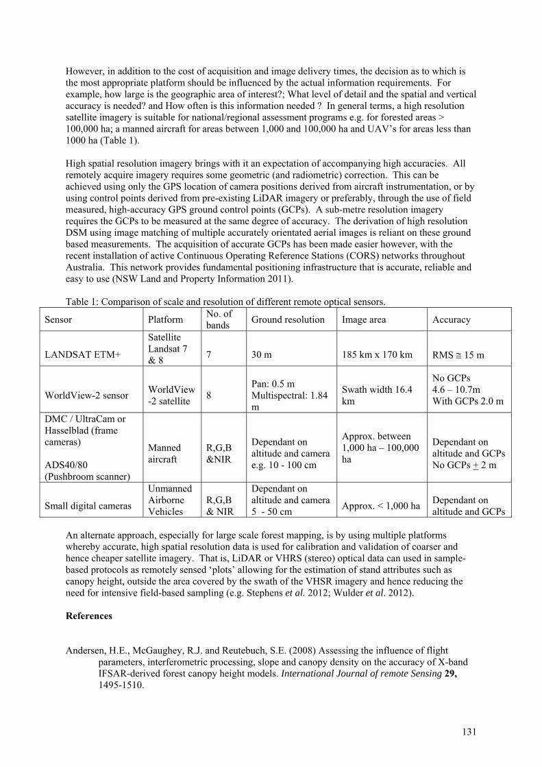
131

However, in addition to the cost of acquisition and image delivery times, the decision as to which is the most appropriate platform should be influenced by the actual information requirements. For example, how large is the geographic area of interest?; What level of detail and the spatial and vertical accuracy is needed? and How often is this information needed ? In general terms, a high resolution satellite imagery is suitable for national/regional assessment programs e.g. for forested areas > 100,000 ha; a manned aircraft for areas between 1,000 and 100,000 ha and UAV’s for areas less than 1000 ha (Table 1). High spatial resolution imagery brings with it an expectation of accompanying high accuracies. All remotely acquire imagery requires some geometric (and radiometric) correction. This can be achieved using only the GPS location of camera positions derived from aircraft instrumentation, or by using control points derived from pre-existing LiDAR imagery or preferably, through the use of field measured, high-accuracy GPS ground control points (GCPs). A sub-metre resolution imagery requires the GCPs to be measured at the same degree of accuracy. The derivation of high resolution DSM using image matching of multiple accurately orientated aerial images is reliant on these ground based measurements. The acquisition of accurate GCPs has been made easier however, with the recent installation of active Continuous Operating Reference Stations (CORS) networks throughout Australia. This network provides fundamental positioning infrastructure that is accurate, reliable and easy to use (NSW Land and Property Information 2011). Table 1: Comparison of scale and resolution of different remote optical sensors.

Sensor Platform No. of bands

Ground resolution Image area Accuracy

LANDSAT ETM+

Satellite Landsat 7 & 8

7

30 m

185 km x 170 km

RMS 15 m

WorldView-2 sensor

WorldView-2 satellite

8

Pan: 0.5 m Multispectral: 1.84 m

Swath width 16.4 km

No GCPs 4.6 – 10.7m With GCPs 2.0 m

DMC / UltraCam or Hasselblad (frame cameras) ADS40/80 (Pushbroom scanner)

Manned aircraft

R,G,B &NIR

Dependant on altitude and camera e.g. 10 - 100 cm

Approx. between 1,000 ha – 100,000 ha

Dependant on altitude and GCPs No GCPs + 2 m

Small digital cameras

Unmanned Airborne Vehicles

R,G,B & NIR

Dependant on altitude and camera 5 - 50 cm

Approx. < 1,000 ha

Dependant on altitude and GCPs

An alternate approach, especially for large scale forest mapping, is by using multiple platforms whereby accurate, high spatial resolution data is used for calibration and validation of coarser and hence cheaper satellite imagery. That is, LiDAR or VHRS (stereo) optical data can used in sample-based protocols as remotely sensed ‘plots’ allowing for the estimation of stand attributes such as canopy height, outside the area covered by the swath of the VHSR imagery and hence reducing the need for intensive field-based sampling (e.g. Stephens et al. 2012; Wulder et al. 2012). References Andersen, H.E., McGaughey, R.J. and Reutebuch, S.E. (2008) Assessing the influence of flight

parameters, interferometric processing, slope and canopy density on the accuracy of X-band IFSAR-derived forest canopy height models. International Journal of remote Sensing 29, 1495-1510.

132

Balzter, H., Luckman, A., Skinner, L., Rowland, C. and Dawson, T. (2007) Observations of stand top height and mean height from interferometric SAR and LiDAR over a conifer plantation at Thetford Forest, UK. International Journal of Remote Sensing 28, 1173-1197.

Bohlin, J., Wallerman, J. and Fransson, J. E.S. (2012) Forest variable estimation using photogrammetric matching of digital aerial images in combination with a high-resolution DEM. Scandinavian Journal of Forest Research 27, 692-699.

Breidenbach, J. and Astrup, R. (2012) Small area estimation of forest attributes in the Norwegian national forest inventory. European Journal Forest Research 131, 1255-1267.

Dandois, J.P. and Ellis, E.C. (2013) High spatial resolution three-dimensional mapping of vegetation spectral dynamics using computer vision. Remote Sensing of Environment 136, 259-276.

Garestier, F., Dubois-Fernandez, P.C and Papathanassiou, K.P. (2008) Pine forest height inversion using single-pass X-band PollnSAR data. IEEE Transactions on Geoscience and Remote Sensing 46, 59-68.

Gobakken, T., Næsset, E. & Bollandsås, O. (2012) Comparing forest stand characteristics predicted from digital aerial photogrammetry and airborne laser scanning. SilviLaser 2012, Sept. 16-19 2012, Vancouver, Canada. Paper No. SL2012-012.

Hobi, M.L. and Ginzler, C. (2012) Accuracy assessment of Digital Surface Models based on WorldView-2 and AD80 stereo remote sensing data. Sensors 12, 6347-6368.

Hirschmüller, H. (2008) Stereo processing by semi-global matching and mutual information. IEEE TPAMI 30, 328-341.

Huang, S., Hager, S.A., Halligan, K.Q., Fairweather, I.S., Swanson, A.K. and Crabtree, R.L. (2009) A comparison of individual tree and forest plot height derived from Lidar and InSAR. Photogrammetric Engineering & Remote Sensing 75, 159-167.

Karjalainen, M., Kankare, V., Vastaranta, M., Holopainen, M. and Hyyppä, J. (2012) Prediction of plot-level forest variables using TerraSAR-X steo SAR data. Remote Sensing of Environment 117, 338-347.

Kelcey, J. and Lucieer, A. (2012) Sensor correction of a 6-band multispectral imaging sensor for UAV remote sensing. Remote Sensing 4, 1462-1493.

Leberl, F., Irschara, A., Pock, T., Meixner, P., Gruber, M., Scholz, S. and Wiechert, A. (2010) Point clouds: Lidar versus 3D vision. Photogrammetric Engineering & Remote Sensing October, 1123-1134.

Lisein, J., Pierrot-Deseilligny, M., Bonnet, S. and Lejeune, P. (2013) A photogrammetric workflow for the creation of a forest canopy height model from small unmanned aerial; system imagery. Forests 4, 922-944.

Næsset, E. (2002) Determination of mean tree height of forest stands by digital photogrammetry. Scandinavian Journal of Forest Research 17, 446-459.

Næsset, E., Gobakken, T., Solberg, S., Gregoire, T.C., Nelson, R. et al. (2011) Model-assisted regional forest biomass estimation using LiDAR and InSAR as auxiliary data: A case study from a boreal forest area. Remote Sensing of Environment 115, 3599-3614.

Nelson, R.F., Hyde, P., Johnson, P., Emessiene, B., Imhoff, M.L., Campbell, R. and Edwards, W. (2007) Investigating RaDAR-LiDAR synergy in a North Carolina pine forest. Remote Sensing of Environment 110, 98-108.

Nurminen, K., Karjalainen, M., Yu, X., Hyyppä, J. And Honkavaara, E. (2013) Performance of dense digital surface models based on image matching in the estimation of plot-level forest variables. ISPRS Journal of Photogrammetry and Remote Sensing 83, 104-115.

Ofner, M., Hirschmugl, M., Raggam, H., Schardt, M. (2006) 3D stereo mapping by means of UltraCamD data. In: Proceedings of the International Workshop on 3D Remote Sensing in Forestry, 14th-15th February, Vienna, pp.353-359.

Persson, H. and Fransson, J.E.S. (2014) Forest variable estimation using radargrammetric processing of TerraSAR-X images in boreal forests. Remote Sensing 6, 2084-2107.

Sexton, J.O., Bax, T., Siqueira, P., Swenson, J.J. and Hensley, S. (2009) a comparison of lidar, radar, and field measurements of canopy height in pine and hardwood forests of southeastern North America. Forest Ecology and Management 257, 1136-1147.

Shamsoddini, A., Trinder, J.C. and Turner, R. (2013) Pine plantation structure mapping using WorldView-2 multispectral image. International Journal of Remote Sensing 34, 3986-4007.

133

Snavely, N., Simon, I., Goesele, M., Szeliski, R., Seitz, S. (2010) Scene reconstruction and visualization from community photo collections. Proceedings of the IEEE 98, 1370-1390.

Solberg, S., Astrup, R., Gobakken, T., Næsset, E. and Weydahl, D.J. (2010) Estimating spruce and pine biomass with interferometric X-band SAR. Remote Sensing of Environment 114, 2353-2360.

Stal, C., Tack, F., DeMaeyer, P., DeWulf, A. and Goossens, R. (2013) Airborne photogrammetry and lidar for DSM extraction and 3D change detection over an urban area – a comparative study. International Journal of Remote Sensing 34, 1087-1110.

Steinmann, K., Mandallz, D., Ginzler, C. and Lanz, A. (2013) Small area estimations of proportion of forest and timber volume combining Lidar data and stereo aerial images with terrestrial data. Scandinavian Journal of Forest Research 28, 373-385.

Stephens, P.R., Kimberley, M.O., Beets, P.N., Paul, T.S.H., Searles, N. Et al. (2012) Airborne scanning LiDAR in a double sampling forest carbon inventory. Remote Sensing of Environment 117, 348-357.

St-Onge, B. , Jumelet, J., Cobello, M. and Véga, C. (2004) Measuring individual tree height using a combination of steophotogrammetry and lidar. Canadian Journal of Forest Research 34, 2122-2130.

St-Onge, B., Vega, C., Fournier, R.A. and Hu, Y. (2008) Mapping canopy height using a combination of digital stereo-photogrammetry and lidar. International Journal of Remote Sensing 29, 3343-3364.

Straub, C., Tian, J., Seitz, R. and Reinartz, P. (2013) Assessment of Cartosat-1 and WorldView-2 stereo imagery in combination with a LiDAR-DTM for timber volume estimation in a highly structured forest in Germany. Forestry 86, 463-473.

Turner, D., Lucieer, A. and Watson, C. (2012) An automated technique for generating georectified mosaics from ultra-high resolution unmanned aerial vehicle (UAV) imagery, based on structure from motion (SfM) point clouds. Remote Sensing 4, 1392-1410.

Vastaranta, M., Niemi, M., Karjalainen, M., Peuhkurinen, J., Kankara, V. Et al. (2014) Prediction of forest stand attributes using TerraSAR-X stereo imagery. Remote Sensing 6, 3227-3246.

Vastaranta, M., Wulder, M.A., White, J.C., Pekkarinen, A., Tuominen, S., Ginzler, C., Kankare, V., Holopainen, M., Hyyppä, J. And Hyyppä, H. (2013) Airborne laser scanning and digital stereo imagery measures of forest structure: comparative results and implications to forest mapping and inventory update. Canadian Journal of Remote Sensing 39, 382-395.

Wallace, L., Lucieer, A., Watson, C. and Turner, D. (2012) Development of a UAV-LiDAR system with application to forest inventory. Remote Sensing 4, 1519-1543.

Wallace, L., Lucieer, A. And Watson, C. (2014a) Evaluating tree detection and segmentation routines on very high resolution UAV LiDAR data. IEEETransactions on Geoscience and Remote Sensing 52, 7619-7628.

Wallace, L., Watson, C. and Lucieer, A. (2014b) Detecting pruning of individual stems using Airborne Laser Scanning data captured from an Unmanned Aerial Vehicle. International Journal of Applied Earth Observation and Geoinformation 30, 76-85.

Wang, J.; Di, K.C.; Li, R. (2005) Evaluation and improvement of geopositioning accuracy of IKONOS stereo imagery. Journal of Surveying Engineering (ASCE) 131, 35-42.

Watt, P.J., Donoghue, D.N.M., McManus and Dunford, R.W. (2006) Predicting forest height from Ikonos, Landsat and LiDAR imagery. International Archives of Photogrammetry, Remote Sensing and Spatial Information Sciences XXXVI – 8/W2, 228-231.

White, J.C., Wulder, M.A., Vastaranta, M/, Coops, N.C., Pitt, D. and Woods, M. (2013) The utility of image-based point clouds for forest inventory: A comparison with airborne laser scanning. Forests 4, 518-536.

Wiechert , A. and Gruber, M. (2009) Photogrammetry versus Lidar: Clearing the air. Professional Surveyor Magazine August, 1-3.

Wijanarto, A. and Osborn, J. (2007) Mapping canopy height of radiata pine plantation in Tasmania, Australia using softcopy photogrammetry. International Journal of Geoinformatics 3, 61-71.

Wulder, M.A., White, J.C., Bater, C.W., Coops, N.C., Hopkinson, C. and Chen, G. (2012) Lidar plots – a new large-area data collection option: context, concepts, and case study. Canadian Journal of Remote Sensing 38, 600-618.

134

Zagalikis, G., Cameron, A.D. and Miller, D.R. (2005) The application of digital photogrammetry and image analysis techniques to derive tree and stand characteristics. Canadian Journal of Forest Research 35, 1224-1237.

Zarco-Tejada, P.J., Diaz-Varela, R., Angileri, V., Loudjani, P. (2014) Tree height quantification using

very high resolution imagery acquired from an unmanned aerial vehicle (UAV) and automatic

3D photo-reconstruction methods. European Journal of Agronomy 55, 89-99.