Project Compass 2.0: A

Preliminary Analysis An Arek’Jaalan Project

Authors: Mark726 and Faulx

A Multidisciplinary Division Research Initiative

1

Project Compass 2.0 Preliminary Analysis

Abstract

Data collected for the revamped Project Compass1 have been used to tentatively locate Anoikis

space in relation to New Eden. According to the data collected, Anoikis space is located

approximately 1250-1350 light years from the center of the New Eden cluster, roughly galactic

southeast from New Eden, in a plane roughly even with New Eden. To date, all Anoikis systems

surveyed have been found within 100 light years of each other, roughly matching New Eden’s

own size. Data were collected through locator services found in all control towers. Using the

principles of trilateration, Project Compass members were able to locate 294 Anoikis systems to

within a few light years of accuracy. The data and this report have been forwarded to Dr. Hilen

Tukoss and Eifyr and Co. for their review and commentary, though given Dr. Tukoss’s recent

absence, it is unknown if official commentary will be forthcoming.

Overview

Anoikis space has been accessible from New Eden since YC 111, when the Seyllin and related

main sequence stellar events somehow marked the opening of unstable wormholes.2 Since then,

there have been extensive attempts to understand the fundamentals of Anoikis, yet many

mysteries about even fundamental aspects remain. Project Compass is an attempt to lay the

foundations of further understanding of Anoikis.

Project Compass attempts to answer the key question of where Anoikis is located compared to

New Eden. Is it located in the same galaxy? The same part of the galaxy? Or across the universe

entirely? Are Anoikis systems even near each other? The revamped Project Compass was

proposed to answer these fundamental questions. The Project was conceived after the Authors

discovered a method by which control towers could be used to determine basic relations between

Anoikis and New Eden, through a process known as trilateration. By using this method, Project

Compass set out to determine the three-dimensional location of Anoikis systems in relation to

New Eden.

Methodology

To make logistics easier for corporations, control tower manufacturers have long included a little

known function to their basic control tower designs: the ability to determine, down to 1/10th of a

light year, the distance to all other anchored control towers owned by a corporation. No other

information is given by this feature. By using a process analogous to that used by scanner probes

to locate certain sites or ships within a solar system, Project Compass utilized this locator

function to determine, as much as possible, the location of Anoikis systems in relation to the

New Eden cluster.

1 The basic project portal is available here.

2 A full review of the events of the Seyllin Incident is available here.

2

In order to locate any point in a three-dimensional system, certain amounts of data are necessary.

One version, called trilateration, requires the coordinates of four reference points, as well as the

distance measurements from those reference points to the location in question. Using these data,

the intersection point of the four spheres (with centers on the reference points, and the measured

distances as radii) can be calculated. There will only be one point where the surfaces of all four

spheres intersect, marking the three-dimensional coordinates of the location in question.3

In order to utilize trilateration, Project Compass anchored four control towers throughout New

Eden to serve as reference points. The systems within which these control towers were anchored

(so-called Control Systems) were then cross-referenced with CONCORD databases that provide

the exact location of all New Eden systems within a common reference grid.4 With the Control

Systems established, researchers were then able to utilize the locator functions of a fifth control

tower in every surveyed Anoikis system to measure distances back to the Control Systems. Each

distance measurement to the Control Systems acts as the radius of one of the four spheres

described above. The intersection point of these four spheres can then be calculated, as described

in Appendix A.

Systems were identified and surveyed as they were discovered, and chains to other Anoikis

systems were followed as far as possible. Once collected, the data were entered into a

spreadsheet created to perform the calculations needed to derive the locations of the Anoikis

systems. A completely separate control tower network was also used to collect a second set of

data. Data were collected until CONCORD removed the functionality on March 13, YC 114.5

Potential Methodological Issues

Two primary problems present themselves in relation to the methodology of this Project. The

first revolves around the soundness of the underlying data. Simply put, it is unclear how the

locator function in the control towers works. Project Compass members have been unable to

determine the process control towers use to almost instantaneously calculate the distance

between themselves and their sister towers, despite apparently being over a thousand light years

away. However, it should be noted that the control towers are accurate within New Eden itself

(and thus can be externally verified utilizing the aforementioned CONCORD databases), lending

at least some credibility to the data. Furthermore, the data itself has been remarkably consistent,

lending further credibility to the data. As discussed below, there is remarkable clustering of

Anoikis systems, showing that at least if the long-distance measurements of the control towers

are in error, all data are probably in error by roughly the same amount, meaning that at least

some parts of the data are still usable. Given these two reasons, the authors believe that the

analysis of the data is certainly worthwhile to present, as long as this caveat is kept in mind.

3 A full overview of the math involved is available in Appendix A.

4 A link to the database used is available here. ((Please note that the static data dump was only used to verify

positions of New Eden systems, as the Project Leads deemed this as something that would be widely available.

Though Anoikis system locations are also contained within the database, they were not utilized for the purposes of

Project Compass. All data analyzed in this report derives solely from data collected from control towers.)) 5 CONCORD apparently only became aware of the locator function’s utility in Anoikis after inquiries by Project

Compass members. After these inquiries, CONCORD announced that they intended to require all control tower

manufacturers to remove the locator function, or at least disable its use in Anoikis. The reasons behind this

announcement are unknown.

3

The second methodological issue is much more practical in nature, and derives from trilateration

itself and the geometry of New Eden. In order to be able to most accurately derive the positions

of Anoikis systems, the Control Systems need as much distance between them as possible along

the x, y, and z axes. A smaller differential means that measurement errors become more

significant, especially along that axis. Due to New Eden’s geometry, this problem becomes most

notable along the y axis. Balancing concerns for security with the needs for maximum distance

yielded four systems suitable as Control Systems for Project Compass’s official towers, located

in Adacyne, Balle, Hemouner, and Kattegaud (Maximum differentials for x, y, and z axes,

respectively, in light-years: 30, 10, 28), with a second set of control towers established in

Gateway, Hemouner (at a separate control tower from Set 1), Horkkisen, and Sakulda

(Maximum differentials for x, y, and z axes, respectively, in light-years: 27, 14, 32), with Set 2

towers being placed entirely in low security space. Notably, due to New Eden’s fairly flat

distribution, Project Compass could only achieve a differential of 10 to 14 light years on the y

axis. This smaller differential could lead to substantial errors in certain system measurements.

However, this concern is balanced by the sheer size of the sample systems (see analysis, below,

for some effects). While individual systems may have an actual y-axis coordinate up to a few

light years different from the estimated coordinate, these errors should smooth out over the

aggregate. Indeed, the clustering of data (again, discussed below) again demonstrates the overall

soundness of the data. Individual data points may be slightly inaccurate, but overall trends can

still be analyzed. Furthermore, the existence of a second data set, even if similarly limited by

New Eden’s geographical limitations, helps to establish the data’s validity.

A third, more minor, methodological issue also presents itself in the form of potential selection

bias. Anoikis systems were selected at random as wormholes to these systems presented

themselves to the Project. Although wormhole topology was assumed fairly random for the

purposes of this Project,6 as-of-yet unidentified patterns may be of significance. Although only

roughly ten-percent of Anoikis systems were analyzed (out of the 2,498 known locus signatures),

all classes of Anoikis were surveyed and hopefully allay fears of selection bias. Adding to this is

the fact that no significant outliers were found from the core cluster of Anoikis that would

suggest the existence of a second cluster of Anoikis space that simply was not found. That does

not indicate the lack of a second cluster, only that it was not found in Project Compass’s surveys.

Experimental Data

Data were obtained from 294 Anoikis systems. Selected data is available in Appendix B while

the full data is available here. Each project member collected a variety of data on each system

surveyed. Beyond the distances to either the primary or secondary set of Control Systems (via a

control tower in each Anoikis system surveyed), the classification of each system as well as any

nearby stellar phenomena were also recorded. The general direction of most phenomenon was

also recorded from galactic north. All data is then entered into a spreadsheet to perform the

necessary calculations. These calculations derive the x, y, and z coordinates of each surveyed

Anoikis systems in light years from the (0, 0, 0) coordinates used by CONCORD. From there,

calculations are performed to find the distance from (0, 0, 0) as well as entered into a graphical

representation of the Anoikis cluster. A listing of the raw data are located in Appendix B.

6 Further research along these lines is ongoing under the auspices of Project Atlas. Details of the research is

available here.

4

Analysis

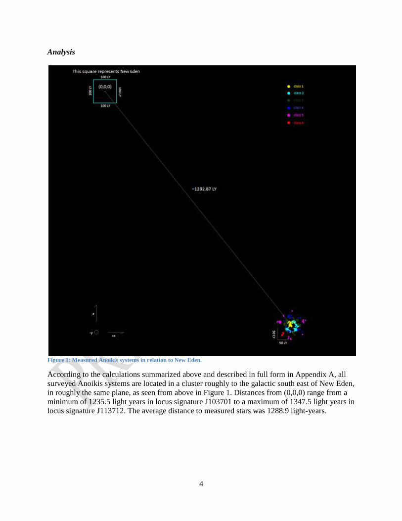
Figure 1: Measured Anoikis systems in relation to New Eden.

According to the calculations summarized above and described in full form in Appendix A, all

surveyed Anoikis systems are located in a cluster roughly to the galactic south east of New Eden,

in roughly the same plane, as seen from above in Figure 1. Distances from (0,0,0) range from a

minimum of 1235.5 light years in locus signature J103701 to a maximum of 1347.5 light years in

locus signature J113712. The average distance to measured stars was 1288.9 light-years.

5

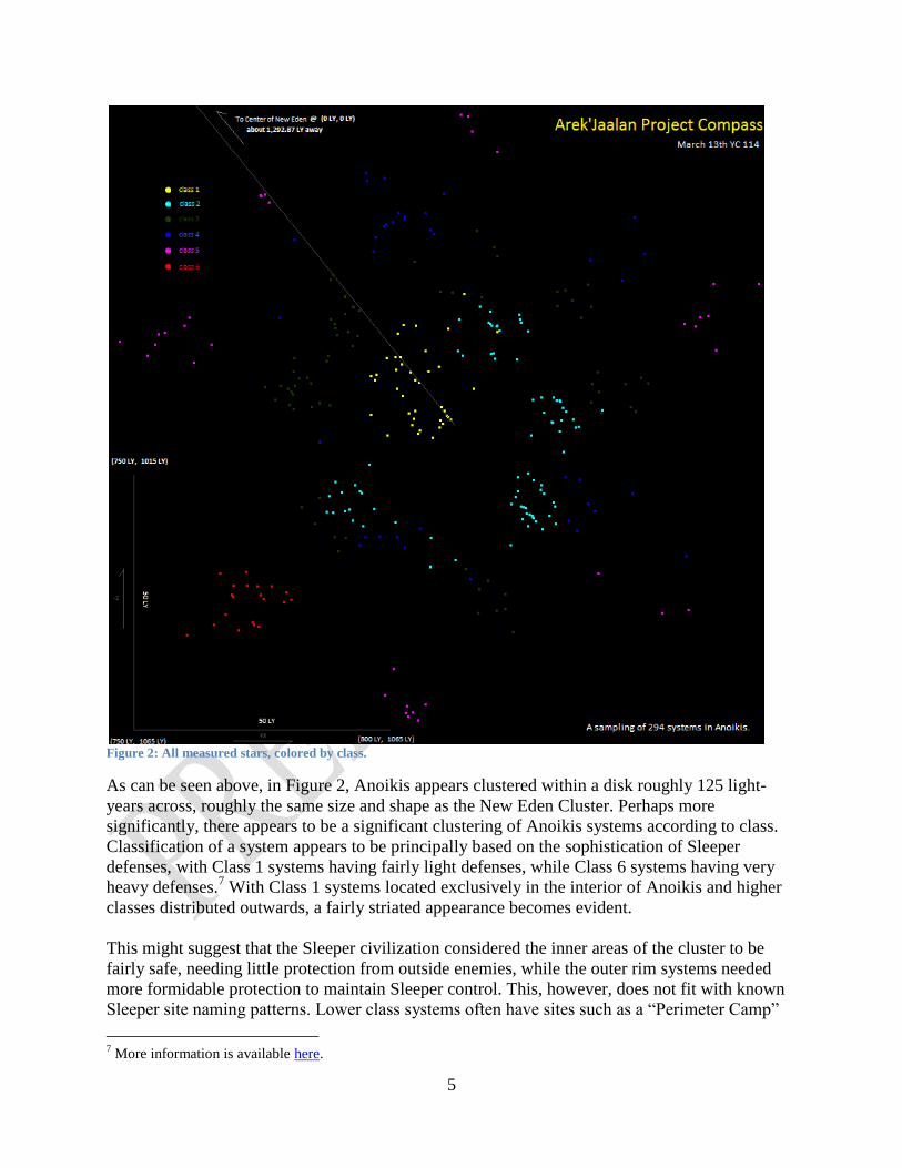
Figure 2: All measured stars, colored by class.

As can be seen above, in Figure 2, Anoikis appears clustered within a disk roughly 125 light-

years across, roughly the same size and shape as the New Eden Cluster. Perhaps more

significantly, there appears to be a significant clustering of Anoikis systems according to class.

Classification of a system appears to be principally based on the sophistication of Sleeper

defenses, with Class 1 systems having fairly light defenses, while Class 6 systems having very

heavy defenses.7 With Class 1 systems located exclusively in the interior of Anoikis and higher

classes distributed outwards, a fairly striated appearance becomes evident.

This might suggest that the Sleeper civilization considered the inner areas of the cluster to be

fairly safe, needing little protection from outside enemies, while the outer rim systems needed

more formidable protection to maintain Sleeper control. This, however, does not fit with known

Sleeper site naming patterns. Lower class systems often have sites such as a “Perimeter Camp”

7 More information is available here.

6

or a “Perimeter Hanger,” while higher class systems might have a “Core Citadel” or a “Core

Bastion.”8 These names, at least, suggest precisely the opposite: that Sleepers considered Class-6

systems to be strongholds while Class 1 systems were considered to be frontier territory. It is

also notable that unlike the other higher classes of wormhole space, Class 6 wormhole systems

are clustered in one area, which raises further questions about the development of Sleeper

civilization (especially given the propensity of Talocan relics to be found in higher classes of

Anoikis).

Another potential theory is that the physical locations of systems should be ignored when

analyzing Sleeper site distributions in favor of examining connections through wormholes. In

that sense, it is notable that Classes 1-3 of Anoikis are easily accessible from New Eden (thus

more easily being considered to be “frontier” or “perimeter” systems if wormholes to New Eden

are considered the frontier), while Classes 4-6 are only very rarely, if ever, accessible from New

Eden. Instead, these higher class systems are generally only accessible through other Anoikis

systems, perhaps lending themselves more easily to being called “core” systems. This

explanation yields even more questions, such as what shut down the original wormhole

networks. Whatever the reason, Sleeper astrocartography certainly warrants further investigation.

Measurement Errors

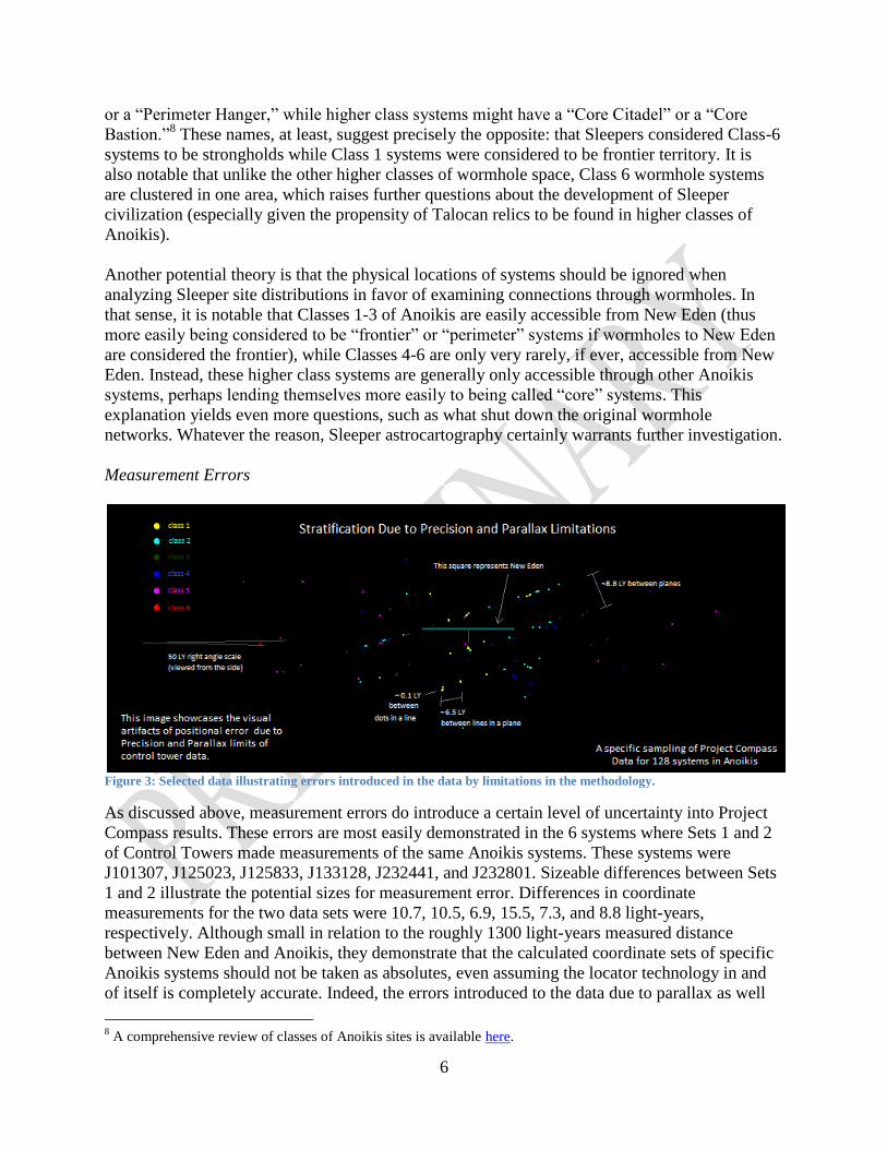
Figure 3: Selected data illustrating errors introduced in the data by limitations in the methodology.

As discussed above, measurement errors do introduce a certain level of uncertainty into Project

Compass results. These errors are most easily demonstrated in the 6 systems where Sets 1 and 2

of Control Towers made measurements of the same Anoikis systems. These systems were

J101307, J125023, J125833, J133128, J232441, and J232801. Sizeable differences between Sets

1 and 2 illustrate the potential sizes for measurement error. Differences in coordinate

measurements for the two data sets were 10.7, 10.5, 6.9, 15.5, 7.3, and 8.8 light-years,

respectively. Although small in relation to the roughly 1300 light-years measured distance

between New Eden and Anoikis, they demonstrate that the calculated coordinate sets of specific

Anoikis systems should not be taken as absolutes, even assuming the locator technology in and

of itself is completely accurate. Indeed, the errors introduced to the data due to parallax as well

8 A comprehensive review of classes of Anoikis sites is available here.

7

as the 1/10th of a light-year sensitivity of the control towers is most evident when the data set is

viewed from a certain angle, as demonstrated in Figure 3, above. The errors in the Compass data

sets are so significant (as compared to the data sets a capsuleer would obtain from using the same

calculations while scanning the system with probes) because the spheres from each of the

Control Towers meet at such acute angles. Regardless, given that Compass’s purpose was only to

provide a rough estimate of Anoikis’s location rather than precise coordinates, the authors

believe that these measurements errors do not hinder Compass’s overall goals.

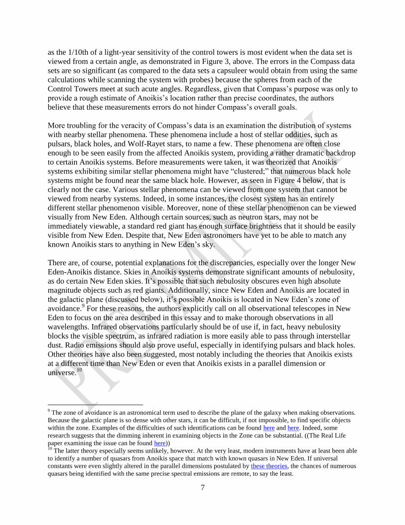
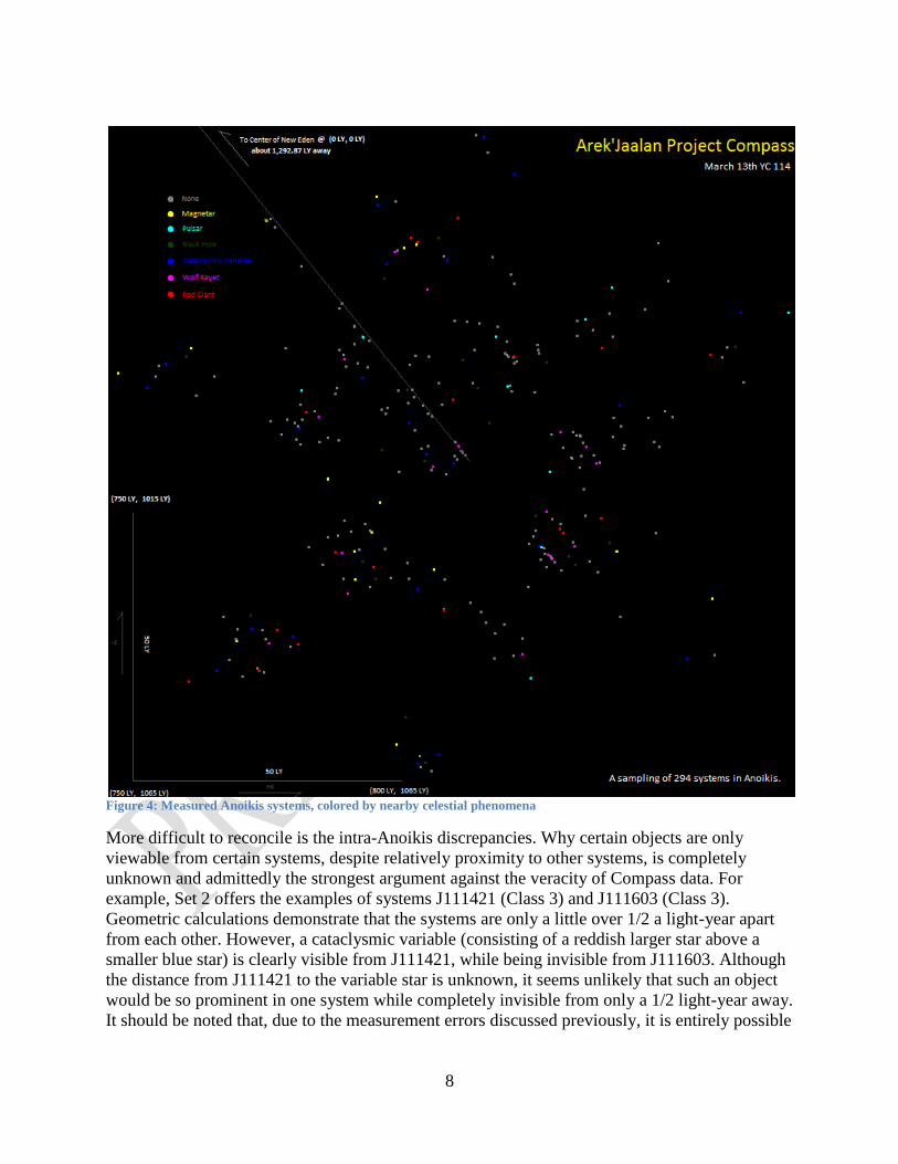
More troubling for the veracity of Compass’s data is an examination the distribution of systems

with nearby stellar phenomena. These phenomena include a host of stellar oddities, such as

pulsars, black holes, and Wolf-Rayet stars, to name a few. These phenomena are often close

enough to be seen easily from the affected Anoikis system, providing a rather dramatic backdrop

to certain Anoikis systems. Before measurements were taken, it was theorized that Anoikis

systems exhibiting similar stellar phenomena might have “clustered;” that numerous black hole

systems might be found near the same black hole. However, as seen in Figure 4 below, that is

clearly not the case. Various stellar phenomena can be viewed from one system that cannot be

viewed from nearby systems. Indeed, in some instances, the closest system has an entirely

different stellar phenomenon visible. Moreover, none of these stellar phenomenon can be viewed

visually from New Eden. Although certain sources, such as neutron stars, may not be

immediately viewable, a standard red giant has enough surface brightness that it should be easily

visible from New Eden. Despite that, New Eden astronomers have yet to be able to match any

known Anoikis stars to anything in New Eden’s sky.

There are, of course, potential explanations for the discrepancies, especially over the longer New

Eden-Anoikis distance. Skies in Anoikis systems demonstrate significant amounts of nebulosity,

as do certain New Eden skies. It’s possible that such nebulosity obscures even high absolute

magnitude objects such as red giants. Additionally, since New Eden and Anoikis are located in

the galactic plane (discussed below), it’s possible Anoikis is located in New Eden’s zone of

avoidance.9 For these reasons, the authors explicitly call on all observational telescopes in New

Eden to focus on the area described in this essay and to make thorough observations in all

wavelengths. Infrared observations particularly should be of use if, in fact, heavy nebulosity

blocks the visible spectrum, as infrared radiation is more easily able to pass through interstellar

dust. Radio emissions should also prove useful, especially in identifying pulsars and black holes.

Other theories have also been suggested, most notably including the theories that Anoikis exists

at a different time than New Eden or even that Anoikis exists in a parallel dimension or

universe.10

9 The zone of avoidance is an astronomical term used to describe the plane of the galaxy when making observations.

Because the galactic plane is so dense with other stars, it can be difficult, if not impossible, to find specific objects

within the zone. Examples of the difficulties of such identifications can be found here and here. Indeed, some

research suggests that the dimming inherent in examining objects in the Zone can be substantial. ((The Real Life

paper examining the issue can be found here)) 10

The latter theory especially seems unlikely, however. At the very least, modern instruments have at least been able

to identify a number of quasars from Anoikis space that match with known quasars in New Eden. If universal

constants were even slightly altered in the parallel dimensions postulated by these theories, the chances of numerous

quasars being identified with the same precise spectral emissions are remote, to say the least.

8

Figure 4: Measured Anoikis systems, colored by nearby celestial phenomena

More difficult to reconcile is the intra-Anoikis discrepancies. Why certain objects are only

viewable from certain systems, despite relatively proximity to other systems, is completely

unknown and admittedly the strongest argument against the veracity of Compass data. For

example, Set 2 offers the examples of systems J111421 (Class 3) and J111603 (Class 3).

Geometric calculations demonstrate that the systems are only a little over 1/2 a light-year apart

from each other. However, a cataclysmic variable (consisting of a reddish larger star above a

smaller blue star) is clearly visible from J111421, while being invisible from J111603. Although

the distance from J111421 to the variable star is unknown, it seems unlikely that such an object

would be so prominent in one system while completely invisible from only a 1/2 light-year away.

It should be noted that, due to the measurement errors discussed previously, it is entirely possible

9

that J111421 and J111603 are significantly farther apart, but these systems were chosen merely

as an example.

While this certainly casts some suspicions on Compass’s data, the authors truly believe that the

Compass data sets are worth releasing and analyzing. Although questions certainly are raised

about the data’s integrity, the data could still present a boon to intrepid researchers. Furthermore,

there could very well be natural explanations for the oddities observed, such as particularly thick

nebulosities that could obscure even closer objects. The authors still believe in the integrity of

the data, but given the potential problems with the data sets, they believe it was important to lay

all issues out in this report, and let the broader scientific community make its own judgments.

Reconciling Results from Original Project Compass

The original Project Compass used a very different methodology in determining the location of

Anoikis based on parallax and stellar spectroscopy.11

Under that methodology, the author

determined that Anoikis was probably located in a halo surrounding the New Eden cluster,

perhaps 500 light years away from New Eden. This conclusion was based on the identification of

a star cluster both in New Eden and Anoikis, nicknamed Orion. Based on changes in Orion’s

configuration from New Eden to Anoikis, the author concluded that the halo hypothesis was the

most reasonable hypothesis.

The halo hypothesis does not precisely match the data gathered in Compass 2.0. Contrary to the

halo hypothesis, the Anoikis Cluster apparently sits approximately 1300 light-years away from

New Eden in a cluster of its own. The reasons for the differences are not entirely clear at this

time. A number of possibilities present themselves, such as some kind of temporal differential

between Anoikis and New Eden. Also, errors in either the identification of Orion or its distance

from New Eden, both mentioned as possibilities in the original Project Compass report, are

possible. Interpretation of the original data may also have been incorrect.

Despite the lack of agreement on why, the question still exists as to which method should be

more trustworthy. On the one hand, the Original Compass methodology relies on known-world

physics and concrete observations. On the other hand, the new methodology relies on actual

numbers from what is seemingly an accurate method of distance determination on at least the

small scale, intra-cluster tests. The authors believe that despite the unknowns in the new

methodology, it is more reliable. The data have been too consistent with each other to be

otherwise. While further observations confirming the 1250-1350 light-year distance would

certainly be helpful, the original methodology’s numbers had enough of a margin of error to end

up possibly fitting the new numbers.

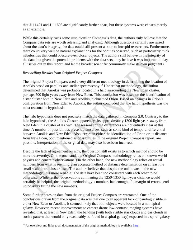
Some further notes on data from the original Project Compass are warranted. One of the

conclusions drawn from the original data was that due to an apparent lack of banding visible in

either New Eden or Anoikis, it seemed likely that both objects were located in a non-spiral

galaxy. However, recent improvements to camera drone low-contrast imaging systems have

revealed that, at least in New Eden, the banding (with both visible star clouds and gas clouds in

such a pattern that would only reasonably be found in a spiral galaxy) expected in a spiral galaxy

11

An overview and links to all documentation of the original methodology is available here.

10

is present. As such, the authors officially retract

that particular conclusion from the Original

Compass report. It is notable, however, that no

such patterns are visible in Anoikis space. This is

not altogether conclusive one way or another, as

many, if not all Anoikis systems, are surrounded

by thick layers of gas themselves, and may thus be

concealing the recently-revealed band patterns.

Further investigations will continue as camera

drone technology continues to improve.

Conclusion

Overall, then, the new Project Compass met the goals laid out in the experimental outline.

Although questions remain about the validity and precision of the data from control tower locator

functions, the data remain too cohesive to not be at least somewhat reliable. Even if the overall

1250-1350 light year distance to New Eden is incorrect due to some unknown error in the locator

function, the fact that the data points are in such close relation to each other suggests that

Anoikis in fact exists as a cluster. Even this revelation alone should provide fascinating insights

into the development of Sleeper and Talocan historical narratives, and hopefully help solve some

of the mysteries of Anoikis.

The data collected during the Project Compass survey was extensive. Although this paper should

be deemed the primary report for Project Compass, the data collected can use further analysis,

especially in the data deemed more secondary in nature (such as the nearby stellar phenomena,

Sleeper and Talocan structures discovered, and the distribution of classes of Anoikis space).

Although the primary purpose of Project Compass – attempting to locate Anoikis in relation to

New Eden – has for now been completed, the rich data sets collected for this project should

prove of use to researchers for some time to come.

Figure 5: A view of the galactic disc as viewed from New

Eden.

Appendix A

A-1

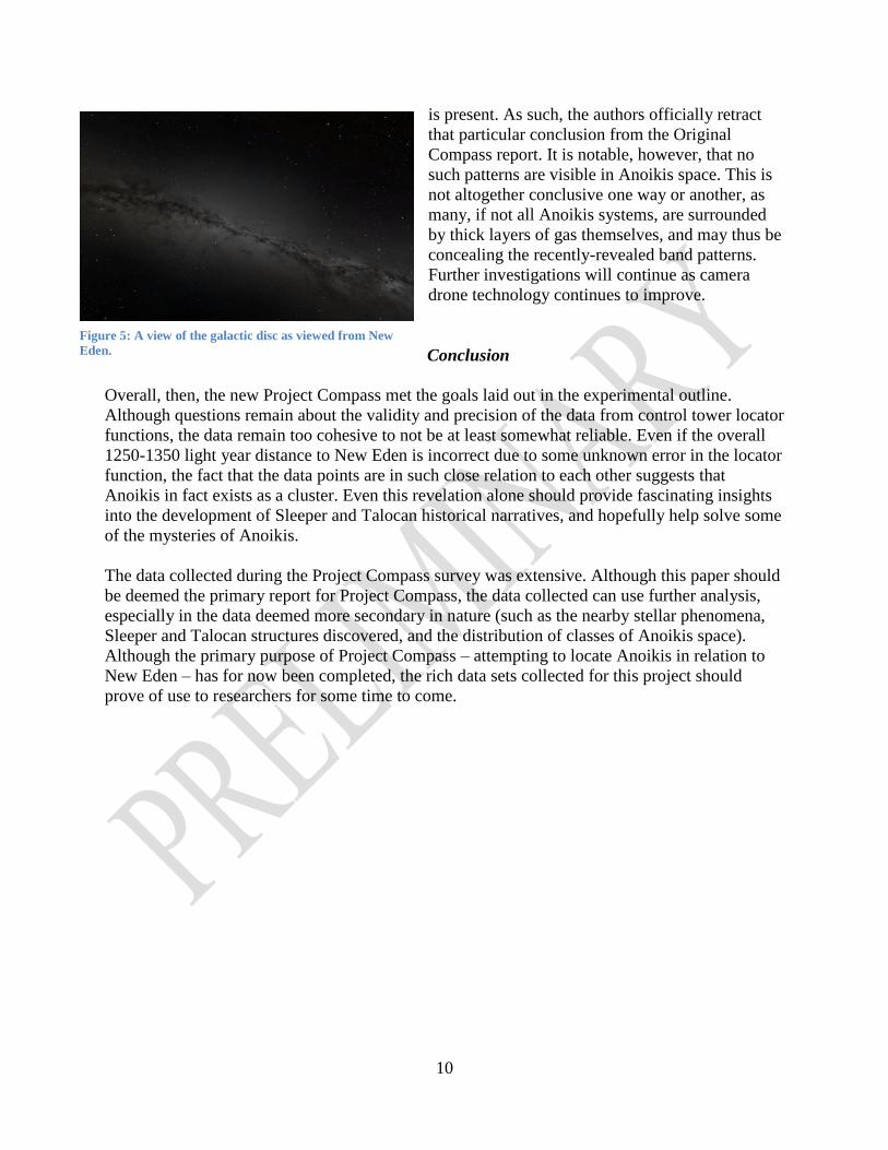
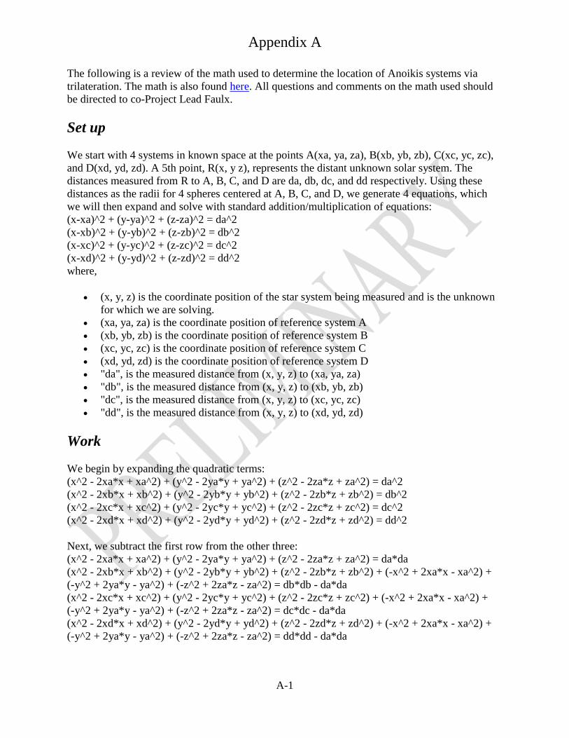
The following is a review of the math used to determine the location of Anoikis systems via

trilateration. The math is also found here. All questions and comments on the math used should

be directed to co-Project Lead Faulx.

Set up

We start with 4 systems in known space at the points A(xa, ya, za), B(xb, yb, zb), C(xc, yc, zc),

and D(xd, yd, zd). A 5th point, R(x, y z), represents the distant unknown solar system. The

distances measured from R to A, B, C, and D are da, db, dc, and dd respectively. Using these

distances as the radii for 4 spheres centered at A, B, C, and D, we generate 4 equations, which

we will then expand and solve with standard addition/multiplication of equations:

(x-xa)^2 + (y-ya)^2 + (z-za)^2 = da^2

(x-xb)^2 + (y-yb)^2 + (z-zb)^2 = db^2

(x-xc)^2 + (y-yc)^2 + (z-zc)^2 = dc^2

(x-xd)^2 + (y-yd)^2 + (z-zd)^2 = dd^2

where,

(x, y, z) is the coordinate position of the star system being measured and is the unknown

for which we are solving.

(xa, ya, za) is the coordinate position of reference system A

(xb, yb, zb) is the coordinate position of reference system B

(xc, yc, zc) is the coordinate position of reference system C

(xd, yd, zd) is the coordinate position of reference system D

"da", is the measured distance from (x, y, z) to (xa, ya, za)

"db", is the measured distance from (x, y, z) to (xb, yb, zb)

"dc", is the measured distance from (x, y, z) to (xc, yc, zc)

"dd", is the measured distance from (x, y, z) to (xd, yd, zd)

Work

We begin by expanding the quadratic terms:

(x^2 - 2xa*x + xa^2) + (y^2 - 2ya*y + ya^2) + (z^2 - 2za*z + za^2) = da^2

(x^2 - 2xb*x + xb^2) + (y^2 - 2yb*y + yb^2) + (z^2 - 2zb*z + zb^2) = db^2

(x^2 - 2xc*x + xc^2) + (y^2 - 2yc*y + yc^2) + (z^2 - 2zc*z + zc^2) = dc^2

(x^2 - 2xd*x + xd^2) + (y^2 - 2yd*y + yd^2) + (z^2 - 2zd*z + zd^2) = dd^2

Next, we subtract the first row from the other three:

(x^2 - 2xa*x + xa^2) + (y^2 - 2ya*y + ya^2) + (z^2 - 2za*z + za^2) = da*da

(x^2 - 2xb*x + xb^2) + (y^2 - 2yb*y + yb^2) + (z^2 - 2zb*z + zb^2) + (-x^2 + 2xa*x - xa^2) +

(-y^2 + 2ya*y - ya^2) + (-z^2 + 2za*z - za^2) = db*db - da*da

(x^2 - 2xc*x + xc^2) + (y^2 - 2yc*y + yc^2) + (z^2 - 2zc*z + zc^2) + (-x^2 + 2xa*x - xa^2) +

(-y^2 + 2ya*y - ya^2) + (-z^2 + 2za*z - za^2) = dc*dc - da*da

(x^2 - 2xd*x + xd^2) + (y^2 - 2yd*y + yd^2) + (z^2 - 2zd*z + zd^2) + (-x^2 + 2xa*x - xa^2) +

(-y^2 + 2ya*y - ya^2) + (-z^2 + 2za*z - za^2) = dd*dd - da*da

Appendix A

A-2

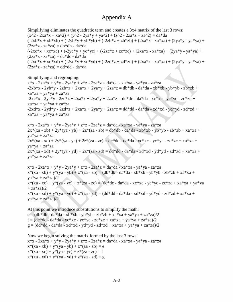
Simplifying eliminates the quadratic term and creates a 3x4 matrix of the last 3 rows:

(x^2 - 2xa*x + xa^2) + (y^2 - 2ya*y + ya^2) + (z^2 - 2za*z + za^2) = da*da

(-2xb*x + xb*xb) + (-2yb*y + yb*yb) + (-2zb*z + zb*zb) + (2xa*x - xa*xa) + (2ya*y - ya*ya) +

(2za*z - za*za) = db*db - da*da

(-2xc*x + xc*xc) + (-2yc*y + yc*yc) + (-2zc*z + zc*zc) + (2xa*x - xa*xa) + (2ya*y - ya*ya) +

(2za*z - za*za) = dc*dc - da*da

(-2xd*x + xd*xd) + (-2yd*y + yd*yd) + (-2zd*z + zd*zd) + (2xa*x - xa*xa) + (2ya*y - ya*ya) +

(2za*z - za*za) = dd*dd - da*da

Simplifying and regrouping:

x*x - 2xa*x + y*y - 2ya*y + z*z - 2za*z = da*da - xa*xa - ya*ya - za*za

-2xb*x - 2yb*y - 2zb*z + 2xa*x + 2ya*y + 2za*z = db*db - da*da - xb*xb - yb*yb - zb*zb +

xa*xa + ya*ya + za*za

-2xc*x - 2yc*y - 2zc*z + 2xa*x + 2ya*y + 2za*z = dc*dc - da*da - xc*xc - yc*yc - zc*zc +

xa*xa + ya*ya + za*za

-2xd*x - 2yd*y - 2zd*z + 2xa*x + 2ya*y + 2za*z = dd*dd - da*da - xd*xd - yd*yd - zd*zd +

xa*xa + ya*ya + za*za

x*x - 2xa*x + y*y - 2ya*y + z*z - 2za*z = da*da - xa*xa - ya*ya - za*za

2x*(xa - xb) + 2y*(ya - yb) + 2z*(za - zb) = db*db - da*da - xb*xb - yb*yb - zb*zb + xa*xa +

ya*ya + za*za

2x*(xa - xc) + 2y*(ya - yc) + 2z*(za - zc) = dc*dc - da*da - xc*xc - yc*yc - zc*zc + xa*xa +

ya*ya + za*za

2x*(xa - xd) + 2y*(ya - yd) + 2z*(za - zd) = dd*dd - da*da - xd*xd - yd*yd - zd*zd + xa*xa +

ya*ya + za*za

x*x - 2xa*x + y*y - 2ya*y + z*z - 2za*z = da*da - xa*xa - ya*ya - za*za

x*(xa - xb) + y*(ya - yb) + z*(za - zb) = (db*db - da*da - xb*xb - yb*yb - zb*zb + xa*xa +

ya*ya + za*za)/2

x*(xa - xc) + y*(ya - yc) + z*(za - zc) = (dc*dc - da*da - xc*xc - yc*yc - zc*zc + xa*xa + ya*ya

+ za*za)/2

x*(xa - xd) + y*(ya - yd) + z*(za - zd) = (dd*dd - da*da - xd*xd - yd*yd - zd*zd + xa*xa +

ya*ya + za*za)/2

At this point we introduce substitutions to simplify the math:

e = (db*db - da*da - xb*xb - yb*yb - zb*zb + xa*xa + ya*ya + za*za)/2

f = (dc*dc - da*da - xc*xc - yc*yc - zc*zc + xa*xa + ya*ya + za*za)/2

g = (dd*dd - da*da - xd*xd - yd*yd - zd*zd + xa*xa + ya*ya + za*za)/2

Now we begin solving the matrix formed by the last 3 rows:

x*x - 2xa*x + y*y - 2ya*y + z*z - 2za*z = da*da - xa*xa - ya*ya - za*za

x*(xa - xb) + y*(ya - yb) + z*(za - zb) = e

x*(xa - xc) + y*(ya - yc) + z*(za - zc) = f

x*(xa - xd) + y*(ya - yd) + z*(za - zd) = g

Appendix A

A-3

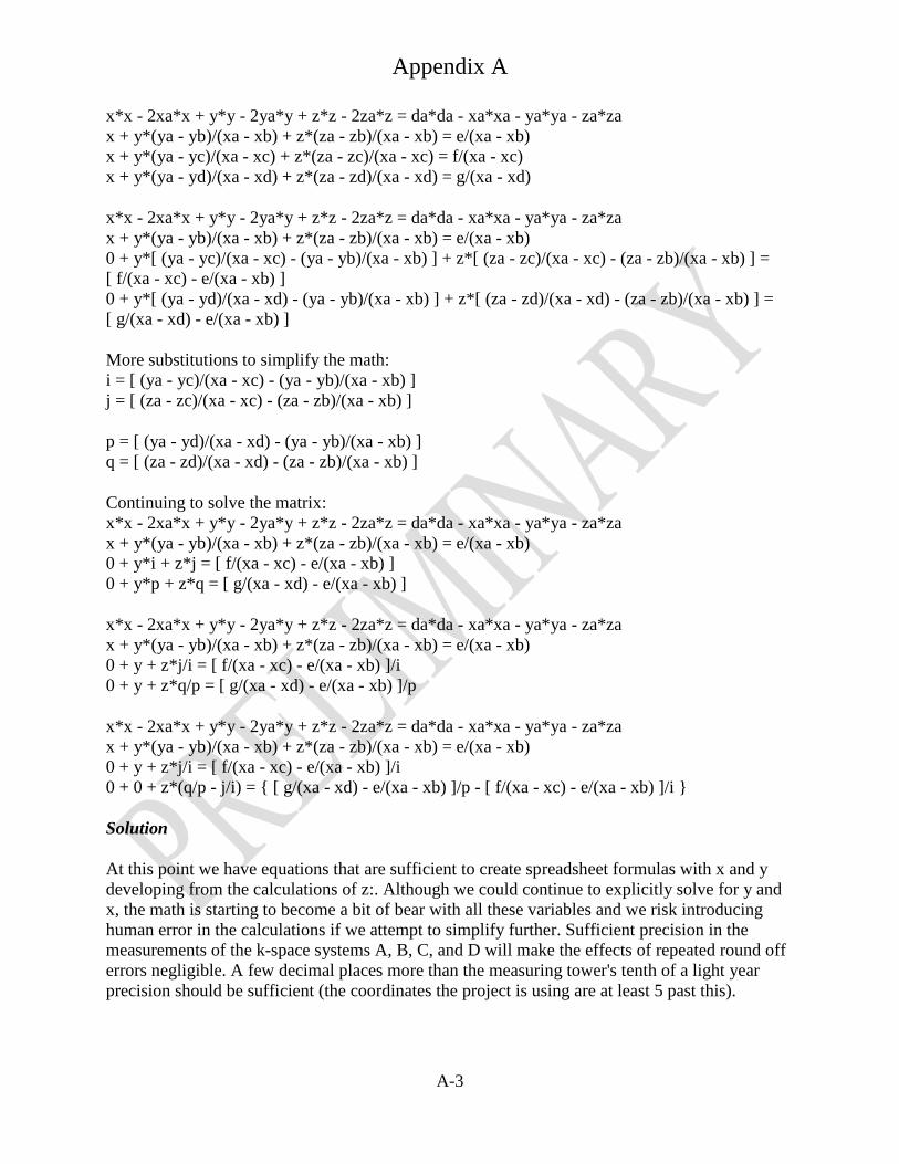
x*x - 2xa*x + y*y - 2ya*y + z*z - 2za*z = da*da - xa*xa - ya*ya - za*za

x + y*(ya - yb)/(xa - xb) + z*(za - zb)/(xa - xb) = e/(xa - xb)

x + y*(ya - yc)/(xa - xc) + z*(za - zc)/(xa - xc) = f/(xa - xc)

x + y*(ya - yd)/(xa - xd) + z*(za - zd)/(xa - xd) = g/(xa - xd)

x*x - 2xa*x + y*y - 2ya*y + z*z - 2za*z = da*da - xa*xa - ya*ya - za*za

x + y*(ya - yb)/(xa - xb) + z*(za - zb)/(xa - xb) = e/(xa - xb)

0 + y*[ (ya - yc)/(xa - xc) - (ya - yb)/(xa - xb) ] + z*[ (za - zc)/(xa - xc) - (za - zb)/(xa - xb) ] =

[ f/(xa - xc) - e/(xa - xb) ]

0 + y*[ (ya - yd)/(xa - xd) - (ya - yb)/(xa - xb) ] + z*[ (za - zd)/(xa - xd) - (za - zb)/(xa - xb) ] =

[ g/(xa - xd) - e/(xa - xb) ]

More substitutions to simplify the math:

i = [ (ya - yc)/(xa - xc) - (ya - yb)/(xa - xb) ]

j = [ (za - zc)/(xa - xc) - (za - zb)/(xa - xb) ]

p = [ (ya - yd)/(xa - xd) - (ya - yb)/(xa - xb) ]

q = [ (za - zd)/(xa - xd) - (za - zb)/(xa - xb) ]

Continuing to solve the matrix:

x*x - 2xa*x + y*y - 2ya*y + z*z - 2za*z = da*da - xa*xa - ya*ya - za*za

x + y*(ya - yb)/(xa - xb) + z*(za - zb)/(xa - xb) = e/(xa - xb)

0 + y*i + z*j = [ f/(xa - xc) - e/(xa - xb) ]

0 + y*p + z*q = [ g/(xa - xd) - e/(xa - xb) ]

x*x - 2xa*x + y*y - 2ya*y + z*z - 2za*z = da*da - xa*xa - ya*ya - za*za

x + y*(ya - yb)/(xa - xb) + z*(za - zb)/(xa - xb) = e/(xa - xb)

0 + y + z*j/i = [ f/(xa - xc) - e/(xa - xb) ]/i

0 + y + z*q/p = [ g/(xa - xd) - e/(xa - xb) ]/p

x*x - 2xa*x + y*y - 2ya*y + z*z - 2za*z = da*da - xa*xa - ya*ya - za*za

x + y*(ya - yb)/(xa - xb) + z*(za - zb)/(xa - xb) = e/(xa - xb)

0 + y + z*j/i = [ f/(xa - xc) - e/(xa - xb) ]/i

0 + 0 + z*(q/p - j/i) = { [ g/(xa - xd) - e/(xa - xb) ]/p - [ f/(xa - xc) - e/(xa - xb) ]/i }

Solution

At this point we have equations that are sufficient to create spreadsheet formulas with x and y

developing from the calculations of z:. Although we could continue to explicitly solve for y and

x, the math is starting to become a bit of bear with all these variables and we risk introducing

human error in the calculations if we attempt to simplify further. Sufficient precision in the

measurements of the k-space systems A, B, C, and D will make the effects of repeated round off

errors negligible. A few decimal places more than the measuring tower's tenth of a light year

precision should be sufficient (the coordinates the project is using are at least 5 past this).

Appendix A

A-4

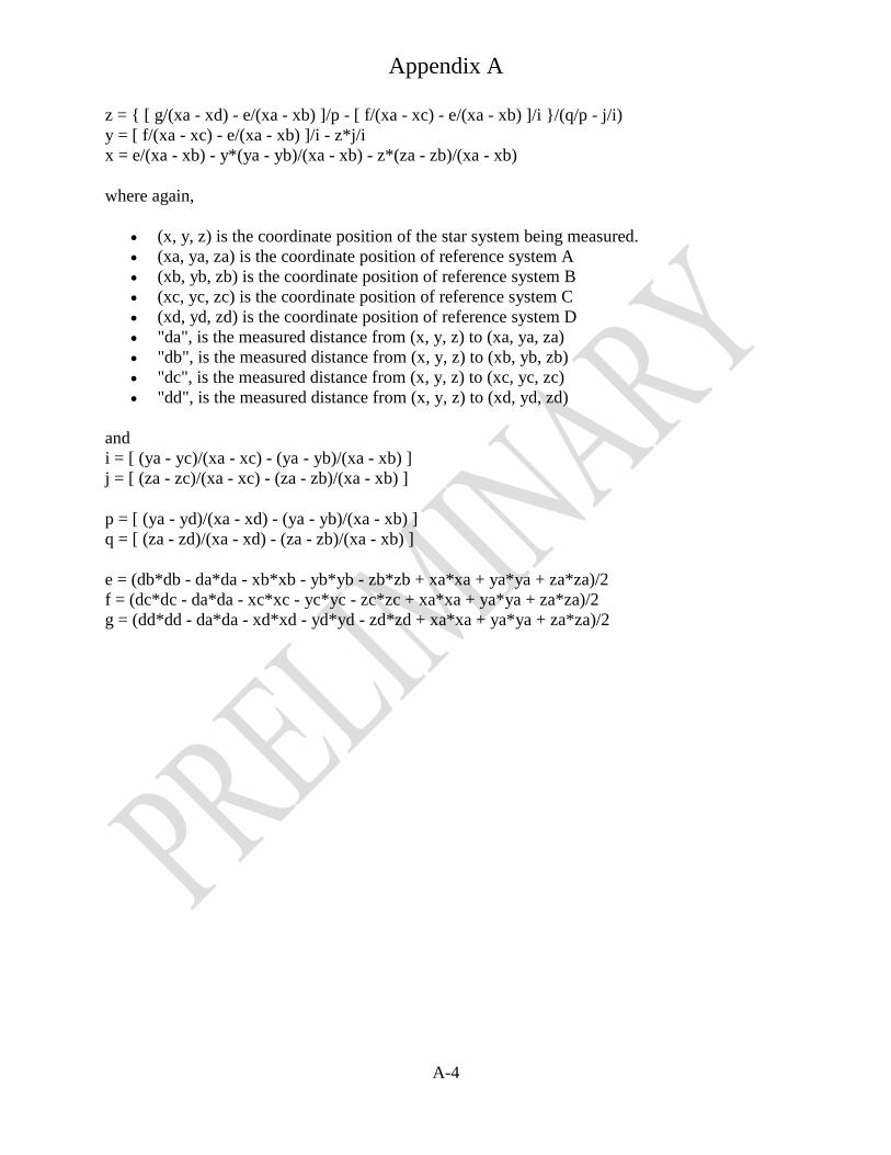
z = { [ g/(xa - xd) - e/(xa - xb) ]/p - [ f/(xa - xc) - e/(xa - xb) ]/i }/(q/p - j/i)

y = [ f/(xa - xc) - e/(xa - xb) ]/i - z*j/i

x = e/(xa - xb) - y*(ya - yb)/(xa - xb) - z*(za - zb)/(xa - xb)

where again,

(x, y, z) is the coordinate position of the star system being measured.

(xa, ya, za) is the coordinate position of reference system A

(xb, yb, zb) is the coordinate position of reference system B

(xc, yc, zc) is the coordinate position of reference system C

(xd, yd, zd) is the coordinate position of reference system D

"da", is the measured distance from (x, y, z) to (xa, ya, za)

"db", is the measured distance from (x, y, z) to (xb, yb, zb)

"dc", is the measured distance from (x, y, z) to (xc, yc, zc)

"dd", is the measured distance from (x, y, z) to (xd, yd, zd)

and

i = [ (ya - yc)/(xa - xc) - (ya - yb)/(xa - xb) ]

j = [ (za - zc)/(xa - xc) - (za - zb)/(xa - xb) ]

p = [ (ya - yd)/(xa - xd) - (ya - yb)/(xa - xb) ]

q = [ (za - zd)/(xa - xd) - (za - zb)/(xa - xb) ]

e = (db*db - da*da - xb*xb - yb*yb - zb*zb + xa*xa + ya*ya + za*za)/2

f = (dc*dc - da*da - xc*xc - yc*yc - zc*zc + xa*xa + ya*ya + za*za)/2

g = (dd*dd - da*da - xd*xd - yd*yd - zd*zd + xa*xa + ya*ya + za*za)/2

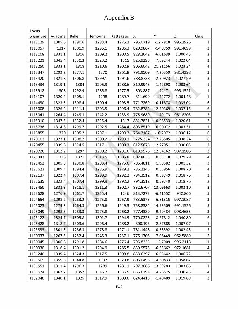
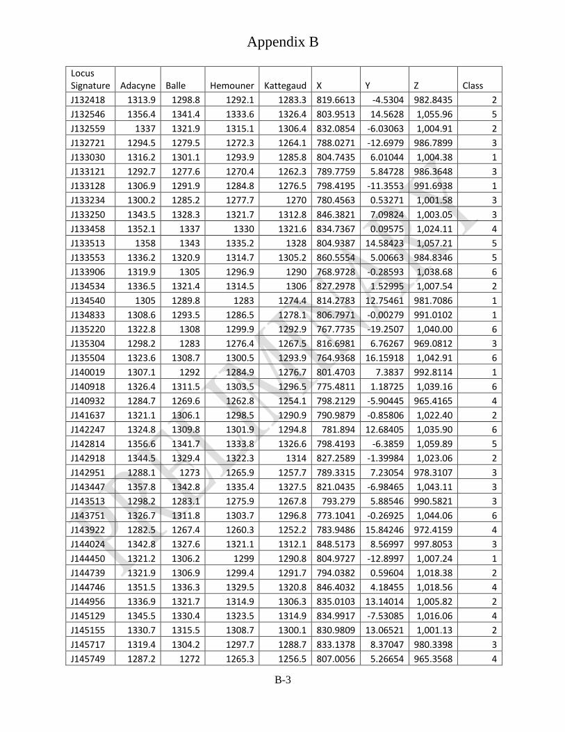
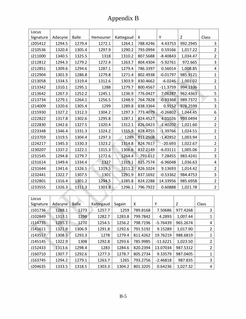
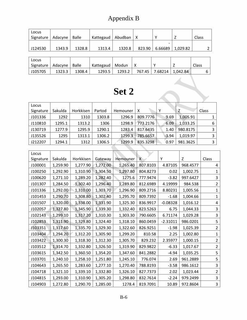
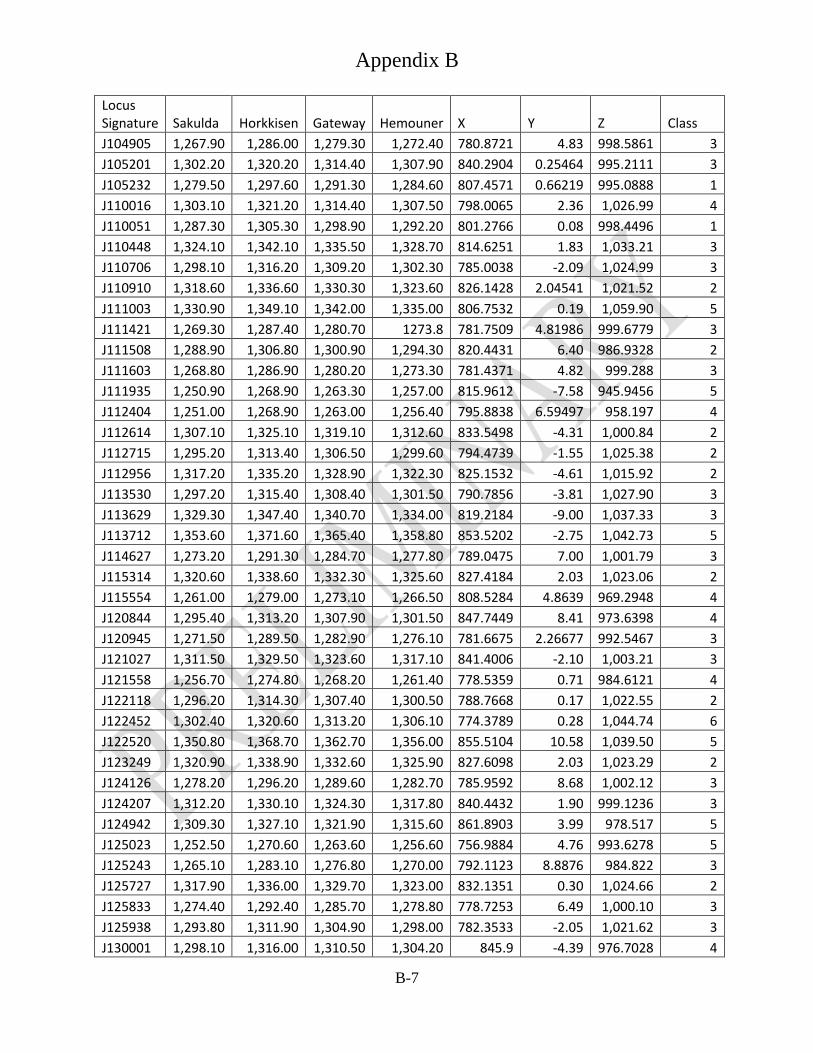
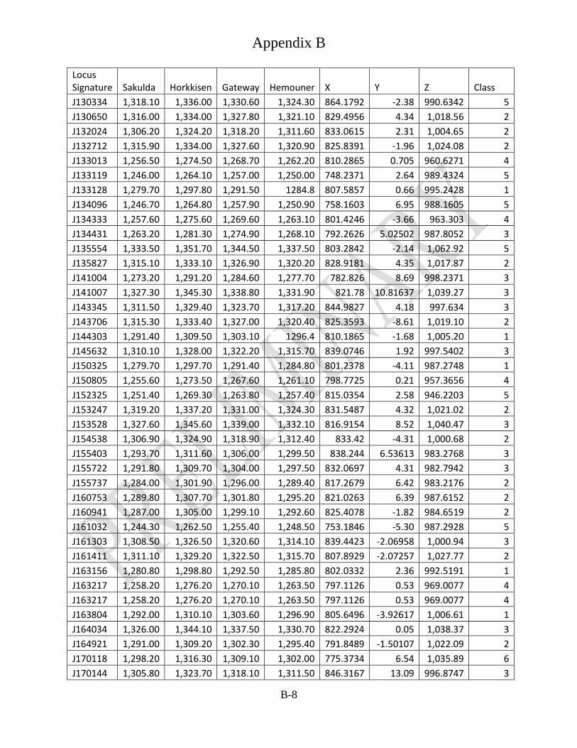
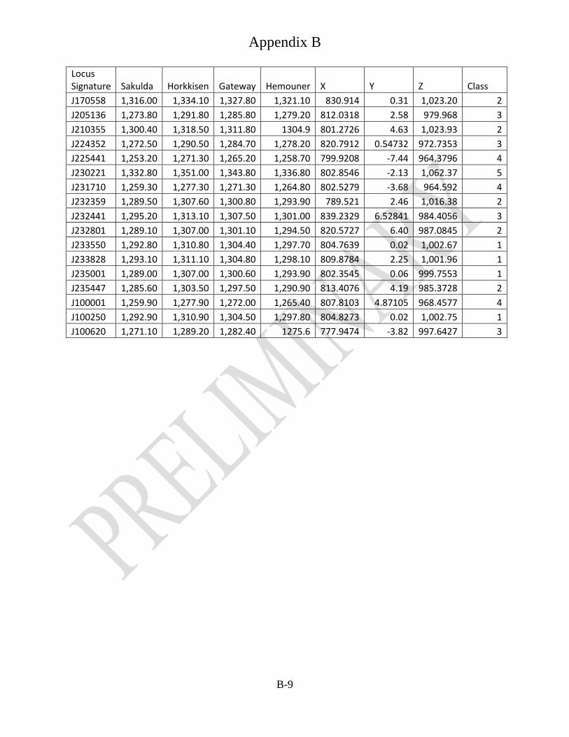
Appendix B

B-1

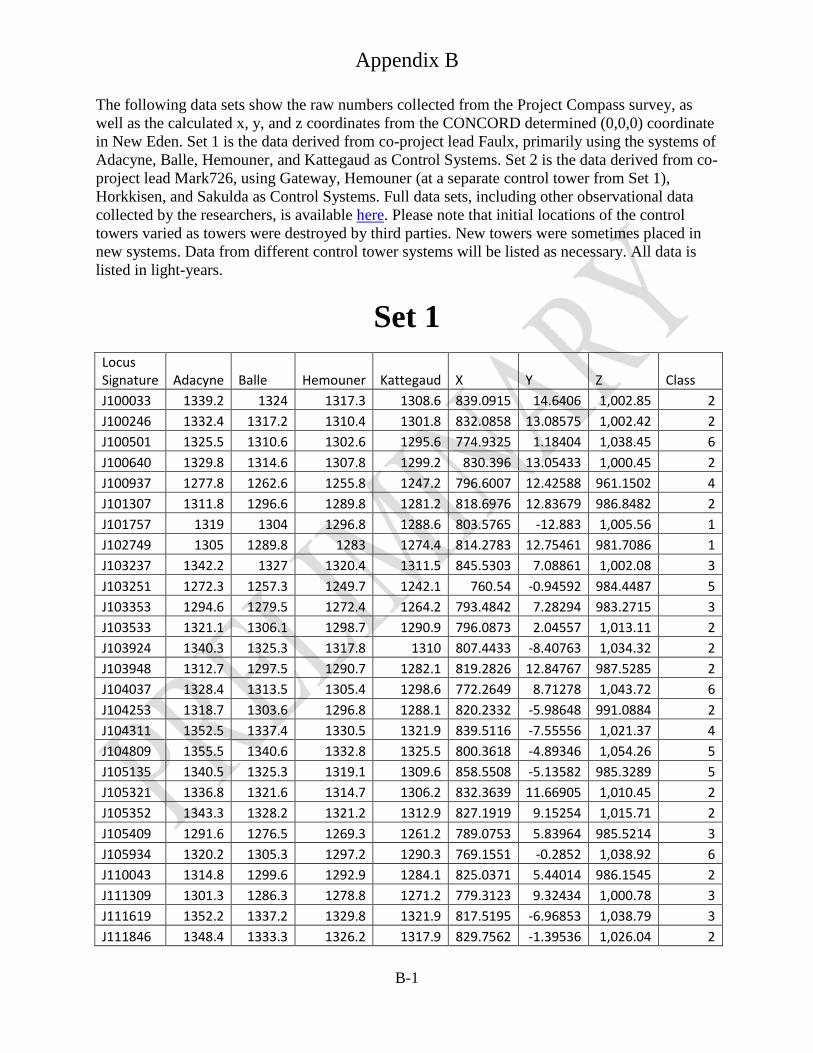
The following data sets show the raw numbers collected from the Project Compass survey, as

well as the calculated x, y, and z coordinates from the CONCORD determined (0,0,0) coordinate

in New Eden. Set 1 is the data derived from co-project lead Faulx, primarily using the systems of

Adacyne, Balle, Hemouner, and Kattegaud as Control Systems. Set 2 is the data derived from co-

project lead Mark726, using Gateway, Hemouner (at a separate control tower from Set 1),

Horkkisen, and Sakulda as Control Systems. Full data sets, including other observational data

collected by the researchers, is available here. Please note that initial locations of the control

towers varied as towers were destroyed by third parties. New towers were sometimes placed in

new systems. Data from different control tower systems will be listed as necessary. All data is

listed in light-years.

Set 1

Locus Signature Adacyne Balle Hemouner Kattegaud X Y Z Class

J100033 1339.2 1324 1317.3 1308.6 839.0915 14.6406 1,002.85 2

J100246 1332.4 1317.2 1310.4 1301.8 832.0858 13.08575 1,002.42 2

J100501 1325.5 1310.6 1302.6 1295.6 774.9325 1.18404 1,038.45 6

J100640 1329.8 1314.6 1307.8 1299.2 830.396 13.05433 1,000.45 2

J100937 1277.8 1262.6 1255.8 1247.2 796.6007 12.42588 961.1502 4

J101307 1311.8 1296.6 1289.8 1281.2 818.6976 12.83679 986.8482 2

J101757 1319 1304 1296.8 1288.6 803.5765 -12.883 1,005.56 1

J102749 1305 1289.8 1283 1274.4 814.2783 12.75461 981.7086 1

J103237 1342.2 1327 1320.4 1311.5 845.5303 7.08861 1,002.08 3

J103251 1272.3 1257.3 1249.7 1242.1 760.54 -0.94592 984.4487 5

J103353 1294.6 1279.5 1272.4 1264.2 793.4842 7.28294 983.2715 3

J103533 1321.1 1306.1 1298.7 1290.9 796.0873 2.04557 1,013.11 2

J103924 1340.3 1325.3 1317.8 1310 807.4433 -8.40763 1,034.32 2

J103948 1312.7 1297.5 1290.7 1282.1 819.2826 12.84767 987.5285 2

J104037 1328.4 1313.5 1305.4 1298.6 772.2649 8.71278 1,043.72 6

J104253 1318.7 1303.6 1296.8 1288.1 820.2332 -5.98648 991.0884 2

J104311 1352.5 1337.4 1330.5 1321.9 839.5116 -7.55556 1,021.37 4

J104809 1355.5 1340.6 1332.8 1325.5 800.3618 -4.89346 1,054.26 5

J105135 1340.5 1325.3 1319.1 1309.6 858.5508 -5.13582 985.3289 5

J105321 1336.8 1321.6 1314.7 1306.2 832.3639 11.66905 1,010.45 2

J105352 1343.3 1328.2 1321.2 1312.9 827.1919 9.15254 1,015.71 2

J105409 1291.6 1276.5 1269.3 1261.2 789.0753 5.83964 985.5214 3

J105934 1320.2 1305.3 1297.2 1290.3 769.1551 -0.2852 1,038.92 6

J110043 1314.8 1299.6 1292.9 1284.1 825.0371 5.44014 986.1545 2

J111309 1301.3 1286.3 1278.8 1271.2 779.3123 9.32434 1,000.78 3

J111619 1352.2 1337.2 1329.8 1321.9 817.5195 -6.96853 1,038.79 3

J111846 1348.4 1333.3 1326.2 1317.9 829.7562 -1.39536 1,026.04 2

Appendix B

B-2

Locus Signature Adacyne Balle Hemouner Kattegaud X Y Z Class

J112129 1305.6 1290.6 1283.4 1275.2 795.0719 -12.7818 995.2926 1

J113057 1317 1301.9 1295.1 1286.3 820.9867 -14.8759 991.4699 2

J113108 1331.1 1316 1309.2 1300.5 828.2642 -6.01639 1,000.45 2

J113221 1345.4 1330.3 1323.2 1315 825.9395 7.69244 1,022.04 2

J113250 1333.1 1318 1310.6 1302.9 806.6042 21.21156 1,023.34 4

J113347 1292.2 1277.1 1270 1261.8 791.9509 7.26359 981.4398 3

J113420 1321.8 1306.8 1299.1 1291.6 788.8738 -2.30923 1,027.59 3

J113434 1319.1 1304 1296.9 1288.6 810.9946 -1.42898 1,003.64 1

J113918 1308 1292.9 1285.8 1277.5 803.887 -1.44171 995.1521 1

J114107 1320.2 1305.1 1298 1289.7 811.699 -1.42772 1,004.48 1

J114430 1323.3 1308.4 1300.4 1293.5 771.7269 10.11878 1,035.04 6

J115008 1326.4 1311.4 1303.5 1296.4 782.8782 12.70369 1,037.15 6

J115041 1264.4 1249.3 1242.2 1233.9 775.9689 -1.49173 961.8203 5

J115310 1347.5 1332.4 1325.4 1317 831.7821 0.08533 1,020.61 2

J115738 1314.8 1299.7 1292.5 1284.4 803.8519 6.00072 1,003.31 1

J115855 1320 1305.2 1297.1 1290.2 764.2187 -10.2972 1,036.12 6

J120103 1323.1 1308.2 1300.2 1293.1 775.334 -7.76505 1,038.24 6

J120455 1339.6 1324.5 1317.1 1309.3 812.5875 12.27951 1,030.05 2

J120726 1312.2 1297 1290.2 1281.6 818.9576 12.84162 987.1506 2

J121347 1336 1321 1313.5 1305.8 802.8633 0.63718 1,029.29 4

J121452 1305.8 1290.8 1283.4 1275.6 786.4811 1.98382 1,001.32 3

J121623 1309.4 1294.4 1286.9 1279.2 786.2145 0.55956 1,008.70 4

J122137 1322.4 1307.4 1299.9 1292.2 794.3512 0.59749 1,018.76 2

J122635 1322.4 1307.4 1299.9 1292.2 794.3512 0.59749 1,018.76 2

J123450 1333.3 1318.1 1311.3 1302.7 832.6707 13.09663 1,003.10 2

J123628 1276.9 1261.7 1255.4 1246 813.7273 -6.41552 942.866 5

J124654 1298.2 1283.2 1275.8 1267.9 783.5373 -6.81315 997.1087 3

J125023 1279.3 1264.3 1256.6 1249.3 758.8384 14.93509 991.1526 5

J125049 1298.3 1283.3 1275.8 1268.2 777.4389 9.29484 998.4655 3

J125122 1324.7 1309.8 1301.7 1294.9 770.0223 8.67812 1,040.80 6

J125428 1318.7 1303.6 1296.4 1288.2 808.193 -2.87885 1,007.97 1

J125833 1301.3 1286.3 1278.8 1271.1 781.1448 0.53592 1,002.43 3

J130037 1267.5 1252.4 1245.3 1237.1 776.1705 7.06449 962.5889 5

J130045 1306.8 1291.8 1284.6 1276.4 795.8335 -12.7909 996.2118 1

J130330 1316.4 1301.2 1294.9 1285.5 839.9573 -6.53662 972.1681 4

J131240 1339.4 1324.3 1317.5 1308.8 833.6397 -6.03642 1,006.72 2

J131509 1359.8 1344.8 1337 1329.8 806.0495 14.60833 1,058.62 5

J131551 1311.4 1296.3 1289 1281.1 797.3086 13.39283 1,003.66 1

J131624 1367.2 1352 1345.2 1336.5 856.6294 4.26575 1,030.45 4

J132048 1340.1 1325 1317.9 1309.6 824.4415 -1.40489 1,019.69 2

Appendix B

B-3

Locus Signature Adacyne Balle Hemouner Kattegaud X Y Z Class

J132418 1313.9 1298.8 1292.1 1283.3 819.6613 -4.5304 982.8435 2

J132546 1356.4 1341.4 1333.6 1326.4 803.9513 14.5628 1,055.96 5

J132559 1337 1321.9 1315.1 1306.4 832.0854 -6.03063 1,004.91 2

J132721 1294.5 1279.5 1272.3 1264.1 788.0271 -12.6979 986.7899 3

J133030 1316.2 1301.1 1293.9 1285.8 804.7435 6.01044 1,004.38 1

J133121 1292.7 1277.6 1270.4 1262.3 789.7759 5.84728 986.3648 3

J133128 1306.9 1291.9 1284.8 1276.5 798.4195 -11.3553 991.6938 1

J133234 1300.2 1285.2 1277.7 1270 780.4563 0.53271 1,001.58 3

J133250 1343.5 1328.3 1321.7 1312.8 846.3821 7.09824 1,003.05 3

J133458 1352.1 1337 1330 1321.6 834.7367 0.09575 1,024.11 4

J133513 1358 1343 1335.2 1328 804.9387 14.58423 1,057.21 5

J133553 1336.2 1320.9 1314.7 1305.2 860.5554 5.00663 984.8346 5

J133906 1319.9 1305 1296.9 1290 768.9728 -0.28593 1,038.68 6

J134534 1336.5 1321.4 1314.5 1306 827.2978 1.52995 1,007.54 2

J134540 1305 1289.8 1283 1274.4 814.2783 12.75461 981.7086 1

J134833 1308.6 1293.5 1286.5 1278.1 806.7971 -0.00279 991.0102 1

J135220 1322.8 1308 1299.9 1292.9 767.7735 -19.2507 1,040.00 6

J135304 1298.2 1283 1276.4 1267.5 816.6981 6.76267 969.0812 3

J135504 1323.6 1308.7 1300.5 1293.9 764.9368 16.15918 1,042.91 6

J140019 1307.1 1292 1284.9 1276.7 801.4703 7.3837 992.8114 1

J140918 1326.4 1311.5 1303.5 1296.5 775.4811 1.18725 1,039.16 6

J140932 1284.7 1269.6 1262.8 1254.1 798.2129 -5.90445 965.4165 4

J141637 1321.1 1306.1 1298.5 1290.9 790.9879 -0.85806 1,022.40 2

J142247 1324.8 1309.8 1301.9 1294.8 781.894 12.68405 1,035.90 6

J142814 1356.6 1341.7 1333.8 1326.6 798.4193 -6.3859 1,059.89 5

J142918 1344.5 1329.4 1322.3 1314 827.2589 -1.39984 1,023.06 2

J142951 1288.1 1273 1265.9 1257.7 789.3315 7.23054 978.3107 3

J143447 1357.8 1342.8 1335.4 1327.5 821.0435 -6.98465 1,043.11 3

J143513 1298.2 1283.1 1275.9 1267.8 793.279 5.88546 990.5821 3

J143751 1326.7 1311.8 1303.7 1296.8 773.1041 -0.26925 1,044.06 6

J143922 1282.5 1267.4 1260.3 1252.2 783.9486 15.84246 972.4159 4

J144024 1342.8 1327.6 1321.1 1312.1 848.5173 8.56997 997.8053 3

J144450 1321.2 1306.2 1299 1290.8 804.9727 -12.8997 1,007.24 1

J144739 1321.9 1306.9 1299.4 1291.7 794.0382 0.59604 1,018.38 2

J144746 1351.5 1336.3 1329.5 1320.8 846.4032 4.18455 1,018.56 4

J144956 1336.9 1321.7 1314.9 1306.3 835.0103 13.14014 1,005.82 2

J145129 1345.5 1330.4 1323.5 1314.9 834.9917 -7.53085 1,016.06 4

J145155 1330.7 1315.5 1308.7 1300.1 830.9809 13.06521 1,001.13 2

J145717 1319.4 1304.2 1297.7 1288.7 833.1378 8.37047 980.3398 3

J145749 1287.2 1272 1265.3 1256.5 807.0056 5.26654 965.3568 4

Appendix B

B-4

Locus Signature Adacyne Balle Hemouner Kattegaud X Y Z Class

J145848 1284.1 1269 1262.3 1253.4 802.1097 -13.1579 962.0719 4

J145931 1316.3 1301.1 1294.4 1285.7 824.1636 14.33824 985.6206 2

J150341 1334.8 1319.6 1312.8 1304.1 835.5256 4.09818 1,005.92 2

J150700 1335.2 1320 1313.2 1304.6 833.9055 13.11959 1,004.53 2

J150745 1308.9 1293.8 1286.7 1278.5 802.6203 7.39821 994.1852 1

J151057 1280.2 1265.3 1257.6 1250.1 758.3336 -12.0475 992.5293 5

J151141 1305.2 1290.1 1282.9 1274.8 797.7374 5.93406 995.9495 1

J151811 1277.6 1262.6 1255 1247.5 762.0485 7.68818 986.9558 5

J152255 1355.7 1340.6 1333.7 1325.2 839.6674 1.5949 1,022.08 4

J152322 1343.7 1328.6 1321.5 1313.3 824.8534 7.67873 1,020.74 2

J153447 1286.2 1270.9 1264.5 1255.3 820.2945 10.57568 955.2391 5

J154900 1297.8 1282.8 1275.4 1267.6 781.4582 1.95153 995.1591 3

J155008 1292.3 1277.2 1270.1 1261.9 792.0148 7.2644 981.5161 3

J155029 1318.1 1302.9 1295.9 1287.6 815.8467 18.91691 999.2127 1

J155338 1330.4 1315.4 1307.8 1300.3 794.916 8.14829 1,027.95 4

J155600 1275.4 1260.5 1252.7 1245.4 751.1108 -4.80485 991.657 5

J155616 1313.1 1298 1291.1 1282.5 814.0713 -7.41646 991.4775 2

J155650 1327.2 1312.3 1304.3 1297.2 777.8388 -7.77876 1,041.47 6

J155935 1314.8 1299.7 1292.5 1284.4 803.8519 6.00072 1,003.31 1

J160307 1309.7 1294.6 1287.6 1279.1 809.3477 -8.84403 993.503 1

J160321 1354.7 1339.6 1332.6 1324.2 836.4066 0.10164 1,026.09 4

J160412 1315.7 1300.6 1293.8 1285 820.1428 -14.8638 990.4867 2

J160715 1316.9 1301.7 1295 1286.2 826.409 5.45334 987.7369 2

J161752 1354.7 1339.6 1332.7 1324.1 840.9321 -7.56333 1,023.04 4

J162159 1321.7 1306.8 1299.2 1291.6 786.5428 -10.8815 1,020.22 2

J162518 1323.5 1308.5 1300.9 1293.3 792.4853 -0.85374 1,024.27 2

J162753 1341.3 1326 1320 1310.3 869.154 7.98664 979.1697 5

J163641 1327.7 1312.7 1305.1 1297.5 795.1058 -0.84618 1,027.53 4

J164104 1292.2 1277.1 1270 1261.7 793.7699 -1.45984 983.0732 3

J164713 1296.7 1281.7 1274.3 1266.4 782.5933 -6.80884 995.9509 3

J164759 1314.2 1299 1292.2 1283.6 820.2574 12.86579 988.6622 1

J165058 1315.7 1300.4 1294.2 1284.8 844.9743 13.77353 967.9951 4

J165901 1310.6 1295.5 1288.4 1280.1 805.5519 -1.43873 997.1398 1

J170305 1285.2 1270.1 1263.2 1254.6 796.0564 -7.31795 970.3116 4

J170511 1298.8 1283.7 1276.4 1268.5 789.3263 13.23233 993.965 3

J171424 1311.7 1296.6 1289.7 1281.1 813.1673 -7.41151 990.4154 2

J171542 1302.3 1287.2 1280.4 1271.7 809.6117 -5.94691 978.7055 3

J171700 1312.7 1297.6 1290.5 1282.3 805.048 7.42884 997.0853 1

J172751 1299.5 1284.5 1277.1 1269.3 782.5256 1.95839 996.4691 3

J204350 1341.5 1326.3 1320.2 1310.5 863.6982 -12.7227 983.0425 5

Appendix B

B-5

Locus Signature Adacyne Balle Hemouner Kattegaud X Y Z Class

J205412 1294.5 1279.4 1272.1 1264.1 788.4246 4.43753 992.2945 3

J210536 1320.4 1305.4 1297.9 1290.2 793.0994 0.59166 1,017.22 2

J211000 1340.5 1325.5 1318 1310.2 807.5688 -8.40843 1,034.47 2

J212812 1294.3 1279.2 1272.4 1263.7 804.4304 -5.92761 972.665 3

J212851 1309.6 1294.6 1287.1 1279.4 786.3397 0.56014 1,008.85 4

J212904 1301.9 1286.8 1279.8 1271.4 802.4938 -0.01797 985.9121 1

J213058 1334.5 1319.4 1312.6 1303.9 830.4662 -6.0246 1,003.02 2

J213342 1310.1 1295.1 1288 1279.7 800.4567 -11.3759 994.1336 1

J213642 1267.3 1252.2 1245.1 1236.9 776.0427 7.06287 962.4363 5

J213734 1279.1 1264.1 1256.5 1248.9 764.7828 -0.93368 989.7372 5

J214009 1320.6 1305.4 1299 1289.8 838.3364 0.9152 978.2599 3

J215930 1327.2 1312.3 1304.2 1297.3 773.4079 -0.26802 1,044.45 6

J222822 1317.8 1302.6 1295.8 1287.1 824.4527 4.01026 993.0494 2

J222830 1342.6 1327.5 1320.4 1312.1 826.0423 -1.40202 1,021.60 2

J223348 1346.4 1331.3 1324.2 1315.9 828.4755 -1.39766 1,024.51 2

J223703 1319.5 1304.4 1297.3 1289 811.2508 -1.42852 1,003.94 1

J224217 1345.3 1330.3 1323.2 1314.8 824.7617 -20.693 1,022.67 2

J230207 1337.2 1322.1 1315.3 1306.6 832.2149 -6.03111 1,005.06 2

J231545 1294.8 1279.7 1272.6 1264.4 793.612 7.28455 983.4241 3

J231614 1349.4 1334.4 1327 1319.1 815.7574 -6.96048 1,036.63 4

J231644 1341.6 1326.5 1319.5 1311.2 826.1024 9.13693 1,014.42 2

J232441 1322.7 1307.5 1301 1291.9 837.1692 -0.53362 984.4753 3

J232801 1316.4 1301.2 1294.5 1285.8 824.2288 14.33956 985.6958 2

J233555 1326.3 1311.3 1303.8 1296.1 796.7922 0.60888 1,021.78 2

Locus Signature Adacyne Balle Kattegaud Sagain X Y Z Class

J101736 1288.1 1273 1257.7 1259 789.8168 7.50686 977.4268 3

J102849 1313.1 1298 1282.7 1283.8 799.7842 4.2893 1,007.44 1

J114735 1285.1 1270 1254.5 1256.2 798.7196 -5.76439 965.2674 4

J141611 1321.9 1306.9 1291.8 1292.6 791.5192 9.15289 1,017.90 2

J143517 1308.5 1293.3 1278 1279.4 811.4262 19.76219 988.6819 1

J145145 1322.9 1308 1292.8 1293.6 785.9985 -11.6221 1,023.50 2

J152433 1313.6 1298.4 1283 1284.6 820.2394 13.07034 987.5312 2

J160710 1307.7 1292.6 1277.3 1278.7 805.2734 9.33579 987.0405 1

J163745 1294.2 1279.1 1263.7 1265 793.2756 -2.46818 987.835 3

J204635 1333.5 1318.5 1303.3 1304.2 801.3205 0.64236 1,027.32 4

Appendix B

B-6

Locus Signature Adacyne Balle Kattegaud Abudban X Y Z Class

J124530 1343.9 1328.8 1313.4 1320.8 823.90 -

6.66689 1,029.82 2

Locus Signature Adacyne Balle Kattegaud Modun X Y Z Class

J105705 1323.3 1308.4 1293.5 1293.2 767.45 7.68214 1,042.84 6

Set 2

Locus Signature Sakulda Horkkisen Partod Hemouner X Y Z Class

J101336 1292 1310 1303.8 1296.9 809.7776 9.69 1,005.91 1

J110810 1295.1 1313.2 1306 1298.9 773.2176 6.09 1,033.25 6

J130719 1277.9 1295.9 1290.1 1283.4 817.6435 1.40 980.8175 3

J135526 1295 1313.1 1306.2 1299.3 785.6657 -3.94 1,019.97 3

J212207 1294.1 1312 1306.5 1299.9 835.3298 0.97 981.3625 3

Locus Signature Sakulda Horkkisen Gateway Hemouner X Y Z Class

J100001 1,259.90 1,277.90 1,272.00 1,265.40 807.8103 4.87105 968.4577 4

J100250 1,292.90 1,310.90 1,304.50 1,297.80 804.8273 0.02 1,002.75 1

J100620 1,271.10 1,289.20 1,282.40 1275.6 777.9474 -3.82 997.6427 3

J101307 1,284.50 1,302.40 1,296.40 1,289.80 812.6989 4.19999 984.538 2

J101336 1,292.00 1,310.00 1,303.70 1,296.90 809.2716 8.80231 1,005.56 1

J101453 1,290.70 1,308.80 1,302.40 1,295.70 809.7392 -1.68 1,004.66 1

J101507 1,320.00 1,338.00 1,331.90 1,325.30 836.9917 -0.08328 1,016.12 4

J102057 1,327.80 1,345.90 1,339.30 1,332.40 823.5263 6.75 1,044.33 3

J102143 1,299.10 1,317.20 1,310.30 1,303.30 790.6605 6.71174 1,029.28 3

J102853 1,311.90 1,329.80 1,324.40 1,318.10 860.0459 -2.31011 986.0201 5

J103351 1,317.60 1,335.70 1,329.30 1,322.60 826.9251 -1.98 1,025.39 2

J103404 1,294.20 1,312.20 1,305.90 1,299.20 810.58 2.25 1,002.80 1

J103422 1,300.30 1,318.30 1,312.30 1,305.70 829.232 2.35977 1,000.15 2

J103512 1,314.70 1,332.80 1,326.50 1,319.90 829.9822 -6.33 1,017.67 2

J103615 1,342.50 1,360.50 1,354.20 1,347.60 841.2882 -4.94 1,035.25 5

J103701 1,240.10 1,258.10 1,251.80 1,245.10 776.074 2.69 961.2889 5

J104643 1,265.50 1,283.60 1,277.10 1,270.40 788.8193 -3.58 986.1612 3

J104718 1,321.10 1,339.10 1,332.80 1,326.10 827.7373 2.02 1,023.44 2

J104815 1,293.00 1,310.90 1,305.20 1,298.80 832.7614 -2.24 979.2499 3

J104903 1,272.80 1,290.70 1,285.00 1278.4 819.7091 10.89 972.8604 3

Appendix B

B-7

Locus Signature Sakulda Horkkisen Gateway Hemouner X Y Z Class

J104905 1,267.90 1,286.00 1,279.30 1,272.40 780.8721 4.83 998.5861 3

J105201 1,302.20 1,320.20 1,314.40 1,307.90 840.2904 0.25464 995.2111 3

J105232 1,279.50 1,297.60 1,291.30 1,284.60 807.4571 0.66219 995.0888 1

J110016 1,303.10 1,321.20 1,314.40 1,307.50 798.0065 2.36 1,026.99 4

J110051 1,287.30 1,305.30 1,298.90 1,292.20 801.2766 0.08 998.4496 1

J110448 1,324.10 1,342.10 1,335.50 1,328.70 814.6251 1.83 1,033.21 3

J110706 1,298.10 1,316.20 1,309.20 1,302.30 785.0038 -2.09 1,024.99 3

J110910 1,318.60 1,336.60 1,330.30 1,323.60 826.1428 2.04541 1,021.52 2

J111003 1,330.90 1,349.10 1,342.00 1,335.00 806.7532 0.19 1,059.90 5

J111421 1,269.30 1,287.40 1,280.70 1273.8 781.7509 4.81986 999.6779 3

J111508 1,288.90 1,306.80 1,300.90 1,294.30 820.4431 6.40 986.9328 2

J111603 1,268.80 1,286.90 1,280.20 1,273.30 781.4371 4.82 999.288 3

J111935 1,250.90 1,268.90 1,263.30 1,257.00 815.9612 -7.58 945.9456 5

J112404 1,251.00 1,268.90 1,263.00 1,256.40 795.8838 6.59497 958.197 4

J112614 1,307.10 1,325.10 1,319.10 1,312.60 833.5498 -4.31 1,000.84 2

J112715 1,295.20 1,313.40 1,306.50 1,299.60 794.4739 -1.55 1,025.38 2

J112956 1,317.20 1,335.20 1,328.90 1,322.30 825.1532 -4.61 1,015.92 2

J113530 1,297.20 1,315.40 1,308.40 1,301.50 790.7856 -3.81 1,027.90 3

J113629 1,329.30 1,347.40 1,340.70 1,334.00 819.2184 -9.00 1,037.33 3

J113712 1,353.60 1,371.60 1,365.40 1,358.80 853.5202 -2.75 1,042.73 5

J114627 1,273.20 1,291.30 1,284.70 1,277.80 789.0475 7.00 1,001.79 3

J115314 1,320.60 1,338.60 1,332.30 1,325.60 827.4184 2.03 1,023.06 2

J115554 1,261.00 1,279.00 1,273.10 1,266.50 808.5284 4.8639 969.2948 4

J120844 1,295.40 1,313.20 1,307.90 1,301.50 847.7449 8.41 973.6398 4

J120945 1,271.50 1,289.50 1,282.90 1,276.10 781.6675 2.26677 992.5467 3

J121027 1,311.50 1,329.50 1,323.60 1,317.10 841.4006 -2.10 1,003.21 3

J121558 1,256.70 1,274.80 1,268.20 1,261.40 778.5359 0.71 984.6121 4

J122118 1,296.20 1,314.30 1,307.40 1,300.50 788.7668 0.17 1,022.55 2

J122452 1,302.40 1,320.60 1,313.20 1,306.10 774.3789 0.28 1,044.74 6

J122520 1,350.80 1,368.70 1,362.70 1,356.00 855.5104 10.58 1,039.50 5

J123249 1,320.90 1,338.90 1,332.60 1,325.90 827.6098 2.03 1,023.29 2

J124126 1,278.20 1,296.20 1,289.60 1,282.70 785.9592 8.68 1,002.12 3

J124207 1,312.20 1,330.10 1,324.30 1,317.80 840.4432 1.90 999.1236 3

J124942 1,309.30 1,327.10 1,321.90 1,315.60 861.8903 3.99 978.517 5

J125023 1,252.50 1,270.60 1,263.60 1,256.60 756.9884 4.76 993.6278 5

J125243 1,265.10 1,283.10 1,276.80 1,270.00 792.1123 8.8876 984.822 3

J125727 1,317.90 1,336.00 1,329.70 1,323.00 832.1351 0.30 1,024.66 2

J125833 1,274.40 1,292.40 1,285.70 1,278.80 778.7253 6.49 1,000.10 3

J125938 1,293.80 1,311.90 1,304.90 1,298.00 782.3533 -2.05 1,021.62 3

J130001 1,298.10 1,316.00 1,310.50 1,304.20 845.9 -4.39 976.7028 4

Appendix B

B-8

Locus Signature Sakulda Horkkisen Gateway Hemouner X Y Z Class

J130334 1,318.10 1,336.00 1,330.60 1,324.30 864.1792 -2.38 990.6342 5

J130650 1,316.00 1,334.00 1,327.80 1,321.10 829.4956 4.34 1,018.56 2

J132024 1,306.20 1,324.20 1,318.20 1,311.60 833.0615 2.31 1,004.65 2

J132712 1,315.90 1,334.00 1,327.60 1,320.90 825.8391 -1.96 1,024.08 2

J133013 1,256.50 1,274.50 1,268.70 1,262.20 810.2865 0.705 960.6271 4

J133119 1,246.00 1,264.10 1,257.00 1,250.00 748.2371 2.64 989.4324 5

J133128 1,279.70 1,297.80 1,291.50 1284.8 807.5857 0.66 995.2428 1

J134096 1,246.70 1,264.80 1,257.90 1,250.90 758.1603 6.95 988.1605 5

J134333 1,257.60 1,275.60 1,269.60 1,263.10 801.4246 -3.66 963.303 4

J134431 1,263.20 1,281.30 1,274.90 1,268.10 792.2626 5.02502 987.8052 3

J135554 1,333.50 1,351.70 1,344.50 1,337.50 803.2842 -2.14 1,062.92 5

J135827 1,315.10 1,333.10 1,326.90 1,320.20 828.9181 4.35 1,017.87 2

J141004 1,273.20 1,291.20 1,284.60 1,277.70 782.826 8.69 998.2371 3

J141007 1,327.30 1,345.30 1,338.80 1,331.90 821.78 10.81637 1,039.27 3

J143345 1,311.50 1,329.40 1,323.70 1,317.20 844.9827 4.18 997.634 3

J143706 1,315.30 1,333.40 1,327.00 1,320.40 825.3593 -8.61 1,019.10 2

J144303 1,291.40 1,309.50 1,303.10 1296.4 810.1865 -1.68 1,005.20 1

J145632 1,310.10 1,328.00 1,322.20 1,315.70 839.0746 1.92 997.5402 3

J150325 1,279.70 1,297.70 1,291.40 1,284.80 801.2378 -4.11 987.2748 1

J150805 1,255.60 1,273.50 1,267.60 1,261.10 798.7725 0.21 957.3656 4

J152325 1,251.40 1,269.30 1,263.80 1,257.40 815.0354 2.58 946.2203 5

J153247 1,319.20 1,337.20 1,331.00 1,324.30 831.5487 4.32 1,021.02 2

J153528 1,327.60 1,345.60 1,339.00 1,332.10 816.9154 8.52 1,040.47 3

J154538 1,306.90 1,324.90 1,318.90 1,312.40 833.42 -4.31 1,000.68 2

J155403 1,293.70 1,311.60 1,306.00 1,299.50 838.244 6.53613 983.2768 3

J155722 1,291.80 1,309.70 1,304.00 1,297.50 832.0697 4.31 982.7942 3

J155737 1,284.00 1,301.90 1,296.00 1,289.40 817.2679 6.42 983.2176 2

J160753 1,289.80 1,307.70 1,301.80 1,295.20 821.0263 6.39 987.6152 2

J160941 1,287.00 1,305.00 1,299.10 1,292.60 825.4078 -1.82 984.6519 2

J161032 1,244.30 1,262.50 1,255.40 1,248.50 753.1846 -5.30 987.2928 5

J161303 1,308.50 1,326.50 1,320.60 1,314.10 839.4423 -2.06958 1,000.94 3

J161411 1,311.10 1,329.20 1,322.50 1,315.70 807.8929 -2.07257 1,027.77 2

J163156 1,280.80 1,298.80 1,292.50 1,285.80 802.0332 2.36 992.5191 1

J163217 1,258.20 1,276.20 1,270.10 1,263.50 797.1126 0.53 969.0077 4

J163217 1,258.20 1,276.20 1,270.10 1,263.50 797.1126 0.53 969.0077 4

J163804 1,292.00 1,310.10 1,303.60 1,296.90 805.6496 -3.92617 1,006.61 1

J164034 1,326.00 1,344.10 1,337.50 1,330.70 822.2924 0.05 1,038.37 3

J164921 1,291.00 1,309.20 1,302.30 1,295.40 791.8489 -1.50107 1,022.09 2

J170118 1,298.20 1,316.30 1,309.10 1,302.00 775.3734 6.54 1,035.89 6

J170144 1,305.80 1,323.70 1,318.10 1,311.50 846.3167 13.09 996.8747 3

Appendix B

B-9

Locus Signature Sakulda Horkkisen Gateway Hemouner X Y Z Class

J170558 1,316.00 1,334.10 1,327.80 1,321.10 830.914 0.31 1,023.20 2

J205136 1,273.80 1,291.80 1,285.80 1,279.20 812.0318 2.58 979.968 3

J210355 1,300.40 1,318.50 1,311.80 1304.9 801.2726 4.63 1,023.93 2

J224352 1,272.50 1,290.50 1,284.70 1,278.20 820.7912 0.54732 972.7353 3

J225441 1,253.20 1,271.30 1,265.20 1,258.70 799.9208 -7.44 964.3796 4

J230221 1,332.80 1,351.00 1,343.80 1,336.80 802.8546 -2.13 1,062.37 5

J231710 1,259.30 1,277.30 1,271.30 1,264.80 802.5279 -3.68 964.592 4

J232359 1,289.50 1,307.60 1,300.80 1,293.90 789.521 2.46 1,016.38 2

J232441 1,295.20 1,313.10 1,307.50 1,301.00 839.2329 6.52841 984.4056 3

J232801 1,289.10 1,307.00 1,301.10 1,294.50 820.5727 6.40 987.0845 2

J233550 1,292.80 1,310.80 1,304.40 1,297.70 804.7639 0.02 1,002.67 1

J233828 1,293.10 1,311.10 1,304.80 1,298.10 809.8784 2.25 1,001.96 1

J235001 1,289.00 1,307.00 1,300.60 1,293.90 802.3545 0.06 999.7553 1

J235447 1,285.60 1,303.50 1,297.50 1,290.90 813.4076 4.19 985.3728 2

J100001 1,259.90 1,277.90 1,272.00 1,265.40 807.8103 4.87105 968.4577 4

J100250 1,292.90 1,310.90 1,304.50 1,297.80 804.8273 0.02 1,002.75 1

J100620 1,271.10 1,289.20 1,282.40 1275.6 777.9474 -3.82 997.6427 3