EUROPEAN ORGANIZATION FOR NUCLEAR RESEARCH European Laboratory for Particle Physics

CERN CH - 1211 Geneva 23

Switzerland Geneva, April 2011

sLHC Project Report 0054

Progress Report on SIMULINK Modelling of RF Cavity Control for SPL Extension to LINAC4

Theory and Analysis behind Simulation Results of SPL Model Using

I/Q Components in SIMULINK to Date, Including Lorentz Force Effects and Multiple Cavities Driven by Single Feedback Loop

Matias Hernandez

Wolfgang Höfle

Abstract

In the context of a luminosity upgrade for the LHC within the coming years, works have started on LINAC4 to provide an infrastructure for updating the LHC supplier chain. In order to achieve energy levels and particles per bunch necessary for the expected rate of events at LHC detectors and related experiments, a project proposal is underway for an appended Superconducting Proton LINAC (SPL) that will run from the normal conducting LINAC4 and LP-SPL onto the LHC supplier chain. Thus, the SPL will have two main functions: Firstly, to provide H- beam for injection into the PS2 which is compatible with LHC luminosity. For this purpose the SPL will accelerate the output beam of LINAC4 from 1GeV to 4GeV, removing, at the same time, the necessity for PSB operation in the LHC supply chain. Secondly, it will provide an infrastructure upgradeable to meet the needs of all potential high-power proton users at CERN (EURISOL) and possibly neutrino production facilities. For high-power applications of this nature the SPL will need to provide a 5GeV beam whose time-structure can be tailored to meet the specifications of each application. As of now, the design of the SPL is planned to make use of high-Q, 5-cell superconducting elliptical cavities pulsed at a resonant frequency of 704.4 MHz by multi-megawatt klystrons with a maximum repetition rate of 50 Hz, accelerating a 20/40 mA H beam with a maximum field of approximately 25 MV/m, depending on the output requirements of different applications. In the context of the development of a proposal for this conceptual design by mid-2011, this report consists on the progress to date of a SIMULINK model that follows the design specifications and will provide a useful means to foresee any issues that might arise with construction of the SPL, as well as a relatively precise feel for the costs involved in terms of power consumption and technology.

Acknowledgements: CEA team, in particular O.Piquet (SIMULINK model)

W. Höfle, G. Kotzian, P. Posocco, J. Tuckmantel, D. Valuch. Beams Department, Radio-Frequency Group SPL : This project has received funding from the European Community's Seventh Framework Programme (FP7/2007-2013) under the Grant Agreement no 212114

sLHC Project

Contents

1 Introduction 6

2 RF Cavity Theory 72.1 Cavity Equivalent Circuit . . . . . . . . . . . . . . . . . . . . . . . . 72.2 Coupling Between RF Generator, Cavity and Beam . . . . . . . . . . 10

2.2.1 Steady-State Analysis . . . . . . . . . . . . . . . . . . . . . . 112.2.2 Transient Analysis . . . . . . . . . . . . . . . . . . . . . . . . 15

2.3 Beam loading Theorem . . . . . . . . . . . . . . . . . . . . . . . . . . 20

3 RF Control of a 5-Cell 704.4 MHz Resonant Cavity 253.1 SPL Design and Modes of Operation . . . . . . . . . . . . . . . . . . 253.2 Power Requirements . . . . . . . . . . . . . . . . . . . . . . . . . . . 263.3 Sources of Perturbation . . . . . . . . . . . . . . . . . . . . . . . . . . 313.4 Feedback and Feed-Forward Control . . . . . . . . . . . . . . . . . . . 323.5 Kalman Filtering . . . . . . . . . . . . . . . . . . . . . . . . . . . . . 36

4 SIMULINK I-Q Model for SPL RF Components 414.1 Generator, Generator-Cavity Coupling . . . . . . . . . . . . . . . . . 454.2 Resonant Cavity Model . . . . . . . . . . . . . . . . . . . . . . . . . . 484.3 RF Feedback Loop . . . . . . . . . . . . . . . . . . . . . . . . . . . . 524.4 Dual Cavity Model . . . . . . . . . . . . . . . . . . . . . . . . . . . . 554.5 Graphical User Interface (GUI) . . . . . . . . . . . . . . . . . . . . . 624.6 Full SPL . . . . . . . . . . . . . . . . . . . . . . . . . . . . . . . . . . 66

5 Results of Model Analysis 695.1 Single Cavity (B=1) in the Absence of Lorentz

Detuning . . . . . . . . . . . . . . . . . . . . . . . . . . . . . . . . . . 695.1.1 Open Loop . . . . . . . . . . . . . . . . . . . . . . . . . . . . 695.1.2 Closed Loop . . . . . . . . . . . . . . . . . . . . . . . . . . . . 73

5.2 Single Cavity (B=1) with Lorentz Detuning Effects . . . . . . . . . . 795.2.1 Open Loop . . . . . . . . . . . . . . . . . . . . . . . . . . . . 795.2.2 Closed Loop . . . . . . . . . . . . . . . . . . . . . . . . . . . . 845.2.3 Variation of Source Beam Current: Low and High Power SPL

Operation . . . . . . . . . . . . . . . . . . . . . . . . . . . . . 905.3 Beam Speed Effects . . . . . . . . . . . . . . . . . . . . . . . . . . . . 93

5.3.1 B=1 Cavities . . . . . . . . . . . . . . . . . . . . . . . . . . . 935.3.2 B=0.65 Cavities . . . . . . . . . . . . . . . . . . . . . . . . . . 98

1

5.4 Dual-Cavity Case . . . . . . . . . . . . . . . . . . . . . . . . . . . . . 1035.4.1 The Need for Feed-Forward . . . . . . . . . . . . . . . . . . . 1035.4.2 Dual Cavity with Feed-Forward . . . . . . . . . . . . . . . . . 1075.4.3 Loaded Quality Factor Mismatch . . . . . . . . . . . . . . . . 108

5.5 Full SPL Simulation Results . . . . . . . . . . . . . . . . . . . . . . . 1125.6 Further Analysis and Stability Considerations . . . . . . . . . . . . . 116

6 Conclusion and Outlook 122

Bibliography 124

2

List of Figures

2.1 Pillbox cavity . . . . . . . . . . . . . . . . . . . . . . . . . . . . . . . 72.2 Cavity equivalent circuit . . . . . . . . . . . . . . . . . . . . . . . . . 92.3 Cavity coupled to beam and generator . . . . . . . . . . . . . . . . . 102.4 Steady-state cavity . . . . . . . . . . . . . . . . . . . . . . . . . . . . 112.5 Fourier spectrum relation between RF and DC beam current . . . . . 132.6 Cavity-beam interaction . . . . . . . . . . . . . . . . . . . . . . . . . 162.7 Cavity voltage gradients induced by generator and beam . . . . . . . 182.8 Effect of single bunch passage on cavity voltage . . . . . . . . . . . . 212.9 Voltage decay in detuned cavity . . . . . . . . . . . . . . . . . . . . . 222.10 Overall effect of beam loading on detuned cavity . . . . . . . . . . . . 222.11 Generator-beam power interaction in tuned cavity . . . . . . . . . . . 24

3.1 General SPL design . . . . . . . . . . . . . . . . . . . . . . . . . . . . 253.2 General SPL parameters . . . . . . . . . . . . . . . . . . . . . . . . . 263.3 General cryogenics parameters . . . . . . . . . . . . . . . . . . . . . . 273.4 Transient power in resonant cavity . . . . . . . . . . . . . . . . . . . 283.5 Negative feedback operation . . . . . . . . . . . . . . . . . . . . . . . 333.6 Effects of PID gain on output control performance . . . . . . . . . . . 343.7 Feedback and feed-forward complementary control . . . . . . . . . . . 353.8 Diagram of piezo-electric tuner control . . . . . . . . . . . . . . . . . 353.9 Kalman filtering operation . . . . . . . . . . . . . . . . . . . . . . . . 39

4.1 I/Q equivalence . . . . . . . . . . . . . . . . . . . . . . . . . . . . . . 424.2 SPL 1 cavity control high level diagram . . . . . . . . . . . . . . . . . 434.3 SPL single-cavity control SIMULINK model overview . . . . . . . . . 444.4 Coupler SIMULINK model (1/N) . . . . . . . . . . . . . . . . . . . . 454.5 Circulator SIMULINK model . . . . . . . . . . . . . . . . . . . . . . 454.6 RF generator high level diagram . . . . . . . . . . . . . . . . . . . . . 464.7 RF generator SIMULINK model . . . . . . . . . . . . . . . . . . . . . 474.8 Beam and generator-induced voltage gradients in cavity . . . . . . . . 484.9 Cavity high level diagram with beam loading and Lorentz detuning . 504.10 Cavity SIMULINK model with beam loading and Lorentz detuning . 514.11 PID feedback loop high-level diagram . . . . . . . . . . . . . . . . . . 534.12 PID feedback SIMULINK model . . . . . . . . . . . . . . . . . . . . . 544.13 Vector average block . . . . . . . . . . . . . . . . . . . . . . . . . . . 554.14 PID feedback loop high-level diagram . . . . . . . . . . . . . . . . . . 564.15 PID feedback SIMULINK model . . . . . . . . . . . . . . . . . . . . . 574.16 Kalman filter high-level diagram . . . . . . . . . . . . . . . . . . . . . 58

3

4.17 Kalman filter SIMULINK model . . . . . . . . . . . . . . . . . . . . . 594.18 High-level diagram of piezo-electric tuner control . . . . . . . . . . . . 604.19 SIMULINK diagram of piezo-electric tuner control . . . . . . . . . . . 614.20 Graphical user interface (1-Cavity) . . . . . . . . . . . . . . . . . . . 634.21 Graphical user interface (2-cavities) . . . . . . . . . . . . . . . . . . . 644.22 Graphical user interface (4-cavities) . . . . . . . . . . . . . . . . . . . 654.23 Full SPL high-level diagram . . . . . . . . . . . . . . . . . . . . . . . 674.24 Full SPL SIMULINK implementation diagram . . . . . . . . . . . . . 68

5.1 Cavity voltage magnitude and phase in the absence of Lorentz detun-ing (open loop) . . . . . . . . . . . . . . . . . . . . . . . . . . . . . . 70

5.2 Forward and reflected power in the absence of Lorentz detuning (openloop) . . . . . . . . . . . . . . . . . . . . . . . . . . . . . . . . . . . . 71

5.3 Power phasor diagram for open loop system . . . . . . . . . . . . . . 725.4 Cavity voltage magnitude and phase in the absence of Lorentz detun-

ing (closed loop) . . . . . . . . . . . . . . . . . . . . . . . . . . . . . 745.5 Cavity voltage magnitude detail . . . . . . . . . . . . . . . . . . . . . 755.6 Forward and reflected power in closed loop operation . . . . . . . . . 765.7 Feedback power added . . . . . . . . . . . . . . . . . . . . . . . . . . 775.8 Power phasor diagram for closed loop system . . . . . . . . . . . . . . 785.9 Resonant frequency shift due to Lorentz force cavity deformation . . 795.10 Cavity voltage magnitude and phase with Lorentz detuning (Open

Loop) . . . . . . . . . . . . . . . . . . . . . . . . . . . . . . . . . . . 805.11 Cavity voltage magnitude and phase detail . . . . . . . . . . . . . . . 815.12 Forward and reflected power with Lorentz detuning . . . . . . . . . . 825.13 Power phasor diagram for open loop system . . . . . . . . . . . . . . 835.14 Cavity voltage magnitude and phase with Lorentz detuning (Open

Loop) . . . . . . . . . . . . . . . . . . . . . . . . . . . . . . . . . . . 855.15 Cavity voltage magnitude and phase detail . . . . . . . . . . . . . . . 865.16 Forward and reflected power with Lorentz detuning . . . . . . . . . . 875.17 Feedback power added . . . . . . . . . . . . . . . . . . . . . . . . . . 885.18 Power phasor diagram for closed loop system . . . . . . . . . . . . . . 895.19 Effect of beam current variation on feedback power (matched operation) 905.20 Low-power operation of SPL (power considerations) . . . . . . . . . . 915.21 Effect of beam current variation on feedback loop power consumption

(mismatched operation) . . . . . . . . . . . . . . . . . . . . . . . . . 925.22 Cavity voltage envelope as seem by beams travelling at different

speeds relative to the speed of light . . . . . . . . . . . . . . . . . . . 945.23 Voltage deviation due to suboptimal speed beamloading . . . . . . . . 955.24 Suboptimal beam speed solution using feed-forward power drop at

beam arrival . . . . . . . . . . . . . . . . . . . . . . . . . . . . . . . . 975.25 Cavity voltage magnitude and phase for correct B=0.65 cavity operation 985.26 Forward and reflected power for correct B=0.65 cavity operation . . . 995.27 Additional power due to feedback correction . . . . . . . . . . . . . . 1005.28 Voltage deviation due to suboptimal speed beamloading . . . . . . . . 101

4

5.29 Suboptimal beam speed solution using feed-forward power drop atbeam arrival . . . . . . . . . . . . . . . . . . . . . . . . . . . . . . . . 102

5.30 Cavity voltage magnitude and phase of vector sum output, feedbackloop is ON . . . . . . . . . . . . . . . . . . . . . . . . . . . . . . . . . 104

5.31 Cavity voltage magnitude and phase for cavity 1 . . . . . . . . . . . . 1055.32 Cavity voltage magnitude and phase for cavity 2 . . . . . . . . . . . . 1065.33 Cavity phase for cavities controlled by a single loop, feed-forward

correction is applied . . . . . . . . . . . . . . . . . . . . . . . . . . . 1075.34 Recursively measured frequency corrections . . . . . . . . . . . . . . . 1085.35 Effect of 18k (1.5%) difference between loaded quality factors of res-

onant cavities . . . . . . . . . . . . . . . . . . . . . . . . . . . . . . . 1095.36 Effect of 26.5k (2.2%) difference between loaded quality factors of

resonant cavities . . . . . . . . . . . . . . . . . . . . . . . . . . . . . 1105.37 Probability distribution of energy jitter for different cavity voltage

errors along SPL . . . . . . . . . . . . . . . . . . . . . . . . . . . . . 1115.38 Beam deterioration due to cumulative effect of accelerating voltage

phase deviation . . . . . . . . . . . . . . . . . . . . . . . . . . . . . . 1135.39 Slow feed-forward scheme using small excitation . . . . . . . . . . . . 1145.40 Beam deterioration solution: randomising cumulative phase effects . . 1155.41 Curve fit for cavity voltage difference with varying loaded quality factor1185.42 Curve fit for cavity voltage magnitude difference with varying Lorentz

force detuning . . . . . . . . . . . . . . . . . . . . . . . . . . . . . . . 1185.43 Curve fit for cavity voltage phase difference with varying Lorentz force

detuning . . . . . . . . . . . . . . . . . . . . . . . . . . . . . . . . . . 1195.44 Bode plot of open-loop system . . . . . . . . . . . . . . . . . . . . . . 121

5

Chapter 1

Introduction

In conjunction with the restart of the Large Hadron Collider at CERN, studies on aluminosity upgrade for the machine started in April of 2008. The project, sLHC-PP,is aimed at gradually increasing the luminosity to reach levels up to ten times theoriginal design specifications of the LHC, providing a smooth transition onto a higherdiscovery potential of the synchrotron [1]. In order to achieve these goals, technicalimprovements need to be deployed on several areas of the CERN complex, includingnew focusing magnets in LHC at the experiment regions. CMS and ATLAS, asgeneral purpose detectors, will need to be prepared to record higher luminositycollisions, and finally, the LHC supplier chain will be updated. Construction hasstarted on LINAC4 to cater for this need. The whole project has been divided intoeight areas of interest referred to as Work Packages. WP1, 2, 3 and 4 are concernedwith project management and the coordination of accelerator and detector upgrades.WP5 is investigating protection and safety issues related to the increased radiationdue to higher luminosity, WP6 has been charged with developing the new focusingquadrupole magnets for the interaction areas of the LHC ring, WP7 is in charge ofdeveloping critical components for the injectors such as accelerating cavities and ahadron source, and finally, WP8 will develop the technology necessary for trackingdetectors from the power distribution point of view. Within the scope of workpackage 7, Low-Level Radio Frequency (LLRF) simulations for a new generation ofpulsed electric field superconducting LINAC have been commissioned. The idea isto provide a general idea of the possible setbacks that may arise during constructionand operation, and their solutions. This report is a detailed description of thefield stabilisation solutions when dealing with one or more superconducting cavitiesdriven by a single pulsed klystron from the RF point of view.

6

Chapter 2

RF Cavity Theory

Particle physics arose only a few decades ago following the creation of a devicecapable of reaching far into the nucleus of an atom, and detectors equipped toobserve matter constituting the building blocks of the building blocks of atoms.Particle accelerators have redefined particle physics and as they become increasinglymore powerful, we are able to penetrate deeper into the standard model and possiblyexpand on it. The idea is to accelerate particles to imbue them with energies capableof separating matter, and then make them crash against each other in an infinitelyprecise point to observe with gigantic detectors what comes out of their collision.In order to achieve this, we insert particles into a vacuum tube, using magnetsto ensure they stay within the vacuum, and accelerate them using electric fieldscontained within resonant cavities along the tube. From the point of view of RFpower, we are interested in observing the effects of a time-varying electric field ona beam of particles travelling through a resonant cavity powered by a powerfulgenerator (klystron). With this information, we can design the RF control systemfor a linear accelerator to suit a particular application.

2.1 Cavity Equivalent Circuit

Figure 2.1: Pillbox cavity [2]

Resonant modes of electromagnetic (EM) waves in cavities can be described by

7

resonant R-C-L circuits. For the simplest case, we limit ourselves to the analysis ofa single resonant cavity, which can be closely modelled via a pillbox with perfectelectric conducting walls (a circular waveguide with closed ends). In an ideal case,only a finite number of propagating modes, corresponding to a finite number offrequencies will propagate within the pillbox, in the presence of losses, however, thedelta function frequency response at different modes becomes a narrowband peakaround the resonant frequency for that mode. A measure of the sharpness of thispeak observed after an external excitation is the quality factor (Q) of that particularmode.Q is defined as the ratio of the time-average of the energy W stored within the cavitywalls to the energy loss per cycle.Q0 = ωW

Pdwhere Pd is the dissipated power in the cavity.

Ignoring the effects of losses due to vacuum impurities and surface irregularities(drift tubes), we calculate Q by integrating the power loss of wall currents over thecavity surface and the stored energy over the volume of the cavity

Pd =

∫δV

P′

ddA =1

2

∫δV

√ωµ

2κ|Htan|2dA (2.1)

W =

∫V

wdV =1

2

∫V

(ε

2|~E|2 +

µ

2|~H|2

)dV =

ε

2

∫V

|~E|2dV (2.2)

where P′

d is the energy loss in the cavity walls per unit area due to surface currents, wis stored energy within the cavity, and κ is the conductivity of the material [3]. TheQ factor as defined above is one of the main characteristics of an accelerator cavity,and together with the resonant frequency and shunt impedance, it is possible todescribe the cavity completely from an electrodynamics point of view. The resonantfrequency of a cavity depends mainly on its shape and it is thus too complex tocalculate analytically for all but the simplest of shapes, thus it is found by numericalor experimental methods and usually quoted by designer or manufacturer. The shuntimpedance of an accelerating cavity relates the voltage between two points in thecavity (e.g. between drift tubes) to the power dissipated in the cavity walls:

Rsh =U2

2Pd(circuit) (2.3)

For LINAC purposes, the shunt impedance definition is multiplied by a factor of two;therefore it is important when defining a shunt impedance to specify the conventionapplied. To calculate the shunt impedance, in any case we find the voltage betweentwo points U = |

∫ z2z1Ez(z)|.

This definition does not take into account the speed of the passing beam and itseffect on the accelerating voltage. It is related to the effective shunt impedance byRsh,eff = RshT

2, where the transit-time factor T is given by

T =|∫ z2z1Ez(z)eikzzdz|

|∫ z2z1Ez(z)dz|

(2.4)

8

Here, kz = 2πβλ

is the wavenumber in the direction of acceleration and depends onthe speed of the beam. This means that the shunt impedance is only meaningfulwhen related to a certain beam speed.Rsh,eff is useful to define the characteristic impedance of a resonant cavity, whichis defined as

Rsh(βx)

Q=

1

2ωW

∣∣∣∣ ∫ z2

z1

Ez(z)ei2πβxc

zdz

∣∣∣∣2 (2.5)

For a beam of speed v = βxc.This is a very useful quantity as it depends only on the geometry of the cavity asenergy scales with electric field. Going back to our R-C-L circuit, we know thatwhen a cavity resonates on a certain mode, the time-average of the energy storedin the electric field equals that in the magnetic field. In an RF period, the energyoscillates between magnetic and electric field as is the case with an L-C pair. R wasdefined before and it models the effective shunt impedance due to energy dissipationof the cavity walls [2].

Figure 2.2: Cavity equivalent circuit

If we therefore think of the capacitance as the effect of the electric field on the cavityand the inductance as related to the magnetic field, we find that the average storedenergy in the electric and magnetic fields respectively is given by

WsE =1

4CV 2 WsM =

1

4LI2 (2.6)

whereε

4

∫V

|E|2dV =µ

4

∫V

|H|2dV

At resonance, the total average energy stored is then the addition of both the mag-netic and electric:

Ws = WsE +WsM = 2WsE =1

2CV 2 (2.7)

9

If we take the power dissipated by the equivalent shunt resistance, bearing in mindω0 = 1√

LCwe find Pd = 1

2V 2

Rand therefore (CIRCUIT) Q0 = ω0RC.

Thus, with the knowledge of the quality factor, resonant frequency and the shuntimpedance, it is possible to construct an equivalent circuit for the resonant cavity.

2.2 Coupling Between RF Generator, Cavity and

Beam

Figure 2.3: Cavity coupled to beam and generator [4]

Until now, we have concentrated on the behaviour of a resonant cavity obtainedfrom a closed pillbox with perfectly conducting walls. We are now interested in theeffects on the cavity of coupling to a generator and the passage of beam. We willnow observe how the generator transmission line affects the quality factor of thecavity and how beam passage will induce a drop in the cavity voltage. Thus weintroduce the concept of the cavity to generator coupling factor

β0 =Q0

Qext

(2.8)

which gives rise to the loaded quality factor QL

1

QL

=1

Q0

+1

Qext

(2.9)

In superconducting cavities in particular, the loaded Q is virtually equal to theexternal Q as the unloaded Q is much greater than the external. This means thegenerator to cavity coupling will be of particular importance for the efficient perfor-mance of the system.

10

2.2.1 Steady-State Analysis

To start off, we assume steady-state voltages and currents. In figure 2.4, the beam isrepresented as a current source and the cavity, as previously shown, is equivalent toan L-C-R block, in this case coupled to a transmission line with complex impedanceZ, with an incident current wave (towards the cavity) Ig and a reflected wave Ir [5].

Figure 2.4: Steady-state cavity [5]

The generator emits a wave with frequency ω, which is not necessarily equal to thecavity resonant frequency ω0. We assume all variables are proportional to eiωt. In thecase of imperfect tuning, the frequency difference between the resonant frequencyand the generator frequency can be described as a mismatch between the generatorand the cavity angle in phasor terms. We can define the tuning angle between thegenerator current and cavity voltage as

tan Ψ = 2QL∆ω

ω

for small ∆ω.From transmission line theory, we know V = Z(Ig + Ir) and therefore Ir = V

Z− Ig.

From the circuit and the above equation, we get

ILCR = Ig − Ir − Ib,RF = 2Ig − Ib,RF −V

Z(2.10)

The current across the L-C-R block is also equal to the individual currents flowingthrough the passive components. So we can also say (j and i both refer to

√−1)

ILCR = IC + IL + IR = V

(1

jωL+ jωC +

1

R

)(2.11)

and equating both sides, we get

V

(jωC

(1− 1

ω2LC

)+

1

R+

1

Z

)= 2Ig − Ib,RF (2.12)

11

If ∆ω = ω0 − ω and ∆ω ω and , we can say that , and the equation becomes

V

(− i2∆ωC +

1

R+

1

Z

)= 2Ig − Ib,RF (2.13)

where ω0 = 1√LC

.Now we want to express this in cavity parameters. To find expressions for C, Rand Z, we use the capacitor voltage-capacitance relation, and the effect of a chargetravelling through a resonant cavity (note that all parameters are specified in theirLINAC definition):

∆V =q

C=qω

2

(R

Q

)(LINAC) (2.14)

C =2

ω(R/Q)(LINAC) (2.15)

Using this and the equivalent cavity values for the shunt impedance R and theexternal impedance Z:

R =Q0

2

(R

Q

)(LINAC) (2.16)

Z =Qext

2

(R

Q

)(LINAC) (2.17)

we find the circuit equation using cavity values to be given by the following equation:

V

(− i 2∆ω

ω(R/Q)+

1

(R/Q)

(1

Q0

+1

Qext

))= Ig −

1

2Ib,RF (2.18)

The RF beam current is a complex quantity, and as such can be expressed in termsof real and imaginary parts. For simplicity we can define the complex phase of allwaves such that the cavity voltage V is always purely real (this is not the case forthe model as shown later). Thus the cavity voltage is at the zero degree point inthe complex plane. The synchronous angle φs is the angle of the RF voltage whenthe beam arrives. With LINAC machines, as is the case with electron synchrotrons,we generally operate close to maximum power transmission. This means that thesynchronous angle is defined from the peak value of the RF voltage, i.e φs, LINAC =0. when the cavity voltage and the beam pulse are in-phase, as opposed to theproton synchrotron case, in which the synchronous angle is taken with 90 degreesof difference. Using the LINAC convention:

Ib,RF = |Ib,RF |(cosφs − i sinφs) (2.19)

The complex Fourier spectrum of a bunch train passing through the cavity is givenby a frequency train which, in case of infinitely short bunches, has equal value forall frequencies f = (−∞,∞). The corresponding real spectrum has no negativelines and corresponding frequencies add up, except for the DC term. Hence, the RFterms are twice the DC term, in the case of infinitely short bunches.

12

Figure 2.5: Fourier spectrum relation between RF and DC beam current

Thus Ib,RF = 2Ib,DC , except for finite bunches, in which case the factor 2 will becomelower for higher frequency components. To take this effect into account we add arelative bunch factor fb that is normalised to 1 for infinitely short bunches, so

Ib,RF = 2Ib,DCfb(cosφs − i sinφs) (2.20)

Substituting back into the previous equation, we find complex expressions for thegenerator and the reflected powers:

Ig =

[V

(R/Q)QL

+ Ib,DCfb cosφs, LINAC

]−i[Ib,DCfb sinφs, LINAC + V

2∆ω

ω(R/Q)

] (2.21)

Ir =

[V

(R/Q)

(1

Qext

− 1

Q0

)− Ib,DCfb cosφs, LINAC

]+i

[Ib,DCfb sinφs, LINAC + V

2∆ω

ω(R/Q)

] (2.22)

All equations above are defined using the LINAC convention for synchronous angleand R/Q. The LINAC definition for power, using peak values for current is

Px =1

4RLINAC|Ix|2

and therefore

Pg,r =1

4(R/Q)Qext|Ig,r|2 (2.23)

We can also find optimum detuning and loaded quality factor for the superconduct-ing LINAC case using

∆ωoptω

=−Ib,DCfb sinφs(R/Q)

2V(2.24)

13

QL,opt = Qext,opt =V

(R/Q)Ib,DCfb cosφs(2.25)

The SPL design involves two types of superconducting cavities along the lengthof the LINAC. These are built for beams of β = 0.65 and β = 1. In practice,however, the (heavy) hydrogen ion beam gradually accelerates along the length ofthe accelerator. This means that the beam speed will be mismatched in the majorityof cases with the cavity design. It is thus interesting to investigate the effects ofdifferent speed beamloading on the cavity voltage waveform.For a certain field inside a resonant cavity, the accelerating voltage that the beam”sees” depends on the speed at which it is travelling. We want to see, thus, what thesteady-state voltage of a cavity optimised for beam passage of a certain β0 will be ifwe operate it with a beam of different speed βx, in terms of the original steady-statevoltage. We define the ratio:

αT =VxVo

=T (βx)

T (β0)(2.26)

This ratio relates the accelerating voltage experienced by beams at different speedsfor a given electric field within the cavity. If we recall

Rsh(βx)

Q=

V 2x

2ωW

we can say (R

Q

)x

= α2T

(R

Q

)0

As we know, the forward and reflected currents interacting in a resonant cavityfed by constant generator power with constant beamloading are given by equations(2.21) and (2.22), where all voltages and currents are steady-state (t → ∞). Weassume that all cavities along the LINAC have been optimised for zero reactivebeamloading. This means that the imaginary part of the equation vanishes always,and from now on we only deal with the real parts, thus the generator/reflectedcurrent equations become (for a superconducting LINAC):

Ig =V t→∞

(R/Q)QL

+ Ib,DCfb cosφs (2.27)

Ir =V t→∞

(R/Q)QL

− Ib,DCfb cosφs (2.28)

Now, we optimise the coupling of the cavity for the design beam speed β0 by choosingthe external quality factor

Qext,opt = QL,opt =V t→∞

0

(R/Q)0Ib,DCfb cosφs(2.29)

If we insert (2.29) into (2.27) and (2.28) the generator and reflected currents become

I(0)g = 2Ib,DCfb cosφs I(0)

r = 0 (2.30)

14

We now maintain the same forward power and operate the cavity with a differentbeam. If the forward power is equal for both cases and they are given by (LINAC)

P (0)g =

1

4(R/Q)0QL|I(0)

g |2

P (x)g =

1

4(R/Q)xQL|I(x)

g |2(2.31)

then for (R/Q)x = α2T (R/Q)0, the forward current scales as I

(x)g =

I(0)g

αTwhen QL is

fixed. Bear in mind that all the values for current and voltage are virtual valuesdependent on the beam speed. The only absolute is the power.

The new current then is given by

I(x)g =

I(0)g

αT=

2Ib,DCfb cosφsαT

and equating to (2.27) for a compensated cavity (no reactive beamloading)

2Ib,DCfb cosφsαT

=V t→∞x

(R/Q)xQL

+ Ib,DCfb cosφs

but the external coupling is optimised for the β0 beam. If we insert our originalequation for the optimal loaded quality factor in terms of β0, we get

2Ib,DCfb cosφsαT

=V t→∞x (R/Q)0

V t→∞0 (R/Q)x

Ib,DCfb cosφs + Ib,DCfb cosφs

which means that the steady-state voltages for beams travelling through a resonantcavity fed by constant power at different speeds are related by:

V t→∞x = (2αT − α2

T )V t→∞0 (2.32)

where αT = T (βx)T (β0)

.

2.2.2 Transient Analysis

The superconducting proton LINAC will make use of pulsed generators, and so doesthe model developed for it. Hence, the scope of the project is not limited to steady-state analysis, and so it is that we now let go of our initial assumptions and plungeinto the realm of transient analysis. We begin again from the externally drivenL-C-R circuit. This time we include the external load in the loaded impedance [4].

RL = R||Zext (2.33)

Applying Kirchhoffs current rule

Icav = IRL + IC + IL

15

Figure 2.6: Cavity-beam interaction [4]

and the formulas

IL = V/L ˙IR = 2V /RL˙IC = CV

and translating into cavity values

1

RLC=

ω0

QL

1

LC= ω2

0

we find

V (t) +1

RLCV (t) +

1

LCV (t) =

1

CI(t) (2.34)

V (t) +ω0

QL

V (t) + ω20V (t) =

ω0RL

QL

I(t) (2.35)

The driving current Ig and the Fourier component of the pulsed beam Ib,RF areharmonic with eiωt. We now separate fast RF oscillation from the slowly changingamplitudes and phases of real and imaginary (I/Q) components of the field vector:

V (t) = (Vr(t) + iVi(t))eiωt

I(t) = (Ir(t) + iIi(t))eiωt

(2.36)

We insert this into the differential equation 2.28 and we end with the result

˙VRE + ω1/2VRE + ∆ωVIM = RLω1/2IRE˙VIM + ω1/2VIM −∆ωVRE = RLω1/2IIM

(2.37)

16

Where ω1/2 = ω0

2QLis the half bandwidth of the cavity. The driving current in

steady-state is given by I = 2Ig + Ib,RF . In the case of on-crest acceleration (zerosynchronous angle) for a train of infinitely short bunches passing through a cavityon resonance, we can approximate the resonant frequency component of the beamcurrent to twice its DC value I = 2(Ig− Ib,DC) , bearing in mind the 180 phase shiftof the beam. Filling a cavity with constant power results in an exponential increaseof the cavity voltage

Vg = RLIg

(1− e

−tτ

)where Vg represents the generator-induced cavity voltage and the LINAC conventionis taken for the loaded impedance. Similarly, a beam current injected at time tinjresults in an opposite voltage gradient within the cavity

Vb = −RLIb,DC

(1− e−

1τ

(t−tinj))

where Vb represents the beam-induced cavity voltage and τ = 1ω1/2

= 2QLω0

is the

filling constant of the cavity.The total cavity voltage is a superposition of the beam-induced and generator-induced voltages.

Vcav(t) = RLIg

(1− e

−tτ

)for t < tinj (2.38)

Vcav(t) = RLIg

(1− e

−tτ

)−RLIb,DC

(1− e

−(t−tinj)τ

)for tinj < t < tOFF (2.39)

In the case of superconducting cavities, the generator power is almost entirely trans-ferred to the beam. The injection time can then be chosen to arrive at an immediatesteady-state condition. In other words, if we time the beam in such a way that thepositive voltage gradient induced by the generator is equal to the negative voltagegradient induced by the beam on the cavity, the cavity voltage will remain constantduring beam loading. This can be achieved, for optimal matching and Ig = αIb,DC ,when the cavity field has reached 1− 1

αof its maximum:

tinj = lnα× τ (2.40)

Vcav(t) = RLIg

(1− e−

tτ

)−RLIb,DC

(1− αe−

tτ

)Vcav(t) = RLIg

(1− e−

tτ

)− RLIg

α

(1− αe−

tτ

) (2.41)

Vcav = Vmax

(1− 1

α

), where Vmax = RLIg (LINAC)

Figure 2.7 shows the effect on the cavity voltage of an infinitely short bunch train,with an average current Ib,DC passing through a cavity at the right injection time

17

Figure 2.7: Cavity voltage gradients induced by generator and beam

tinj such that the generator-induced gradient is cancelled by that induced by thebeam.Each infinitely short bunch is seen as an instant drop in the cavity voltage, whilethe generator-induced voltage has a continuous effect on the cavity. When both thebeam and generator are OFF, the cavity voltage decays exponentially.In the last section, we arrived at the conclusion that the beamloading effects interms of cavity voltage and beam acceleration differ depending on the speed of thebeam traversing a resonant cavity with a given electric field. As explained before,the accelerating voltage that a beam “sees” when passing through the resonantcavity will depend on its relativistic β factor, as it will experience a number ofcycles of the RF power. This means, when operating close to relativistic speeds,that beamloading will be weaker for a slower beam than a faster one. For example,a beam travelling at the speed of light will absorb more RF power from the cavitythan a slower one. This will result in a higher beam-induced voltage on the cavityand the steady-state equilibrium voltage inside the cavity will be lower for a givencoupling, forward power, and beam current.The cavity voltage envelope waveform needs to be specified for a certain beamspeed in order to have meaning. Until now, we have assumed a fixed geometricfactor (R/Q), which is expressed for the design beam speed of the cavity. Now, it isinteresting to investigate the transient effects during filling, injection and decay timeof the cavity with different beam speed. We assume again that the aforementionedvoltage envelope is actually the accelerating voltage that a beam travelling with aβ0 speed would experience when passing through the cavity. What happens if adifferent beam of speed βx is present at injection?Before beamloading, the voltage within the cavity can be expressed in terms of anybeam. Thus, if we know the behaviour of V0(t) for a β0 beam during filling, Vx(t)

18

is merely given by αTV0(t), where αT = TxT0

(T is the transit-time factor). In otherwords

V (βx, t) = αTV (β0, t) (2.42)

If the cavity is loaded up to the β0 steady-state voltage, at injection

V (βx, tinj) = αTVt→∞

0 (2.43)

The voltage will remain constant during beamloading (flat-top) for the β0 beam. Fora different beam, a new equilibrium will be reached. The cavity voltage will tendtowards the steady-state voltage for the new beam, and the voltage swing betweeninjection and the new steady-state will be given by V t→∞

x −αTV t→∞0 as seen by the

βx beam. If the new equilibrium voltage V t→∞x = (2αT −α2

T )V t→∞0 , then the voltage

swing during beamloading is

∆Vx = V t→∞x − Vx(tinj) = (2αT − α2

T − αT )V t→∞0 (2.44)

Therefore, the complete voltage envelope as seen by the new beam becomes

Vx(t < tinj) = αTV∞(

1− e−tτ

)(2.45)

Vx(t > tinj) = αTVt→∞

0

[1 + (1− αT )

(1− e

−(t−tinj)τ

)](2.46)

where V ∞ = RL0Ig is the steady-state voltage without beam as would be seen bythe β0 beam, and V t→∞

0 is the design accelerating voltage as seen by the β0 beam.

It is important to note that the above description is somewhat different in the caseof out of phase beam loading. It is important to bear in mind that when the beamarrives with a certain synchronous angle, the beam current is expressed by

Ib,RF = |Ib,RF |(cosφs − i sinφs) (2.47)

and similarly, the generator current is given by

Ig =

[V

(R/Q)QL

+ Ib,DCfb cosφs, LINAC

]−i[Ib,DCfb sinφs, LINAC + V

2∆ω

ω(R/Q)

] (2.48)

This means that the relationship between Ig and Ib becomes

Ig = α Ib,DC

where the underlining represents complex quantities. This means that the injectiontime would have to be complex in order to obtain flat-top operation, which is, ofcourse, physically impossible. In practice this means that the cavity voltage flat-top operation can be optimised with respect to the real part by means of optimal

19

coupling and with respect to the imaginary part by detuning the cavity. For thepurpose of our analysis, the focus is on the real part and thus the effects of flat-topdrift during beam loading due to reactive effects are in practice curbed by a fastfeedback loop in both magnitude and phase, though other methods life pre-detuningor half-detuning have proven successful in the past.

2.3 Beam loading Theorem

Until now, the passage of the beam through a resonant cavity has been representedby a DC current source pulled from the cavity. This is a good approximation andworks well to observe the beam effect on the magnitude of the cavity voltage. In real-ity, however, beam loading consists on the effects of several single bunches (modelledwith infinitely small width) accelerated by a resonant cavity. These bunches not onlyhave an effect in the cavity voltage magnitude, but also its phase. When a beam isperfectly in-phase with the RF voltage in a tuned cavity, the cavity voltage will stayin tune during beam passage, while its amplitude decays, however, the transienteffects of a detuned cavity and the beam synchronous angle remain to be discussed.As we will see during the course of this paper in both theory and practice, a beamthat arrives at the cavity with a synchronous angle φs will asymptotically pull thecavity voltage towards this angle (note that we use the LINAC definition for φs).After the passing of a point charge through a resonant cavity, an induced voltageVbn remains in each resonant mode (for simplicity we will consider the main modeonly). What fraction of Vbn does the charge “see”? We will prove this to be 1

2Vbn.

This result is called the fundamental theorem of beam loading [6]. The fundamentaltheorem of beam loading relates the energy loss by a charge crossing the cavity to theelectromagnetic properties of resonant modes in the cavity computed in the absenceof field. By superposition, the beam-induced voltage in a resonant cavity is the samewhether or not there is a generator-induced voltage already present. We observe theeffect of a charge passing through a cavity, being accelerated by generator-inducedfield present within said cavity. A single bunch passing through a cavity excites afield within it. Taking into account the fundamental resonant mode only, the excitedfield can be expressed as an exponentially decaying sine wave oscillating with thecavity’s resonant frequency ω0. In vector terms, the power delivered to the beam bythe RF, taking into account the beam-induced cavity voltage is given by

Pb,eff = −(~Vg + ~Vb) • ~Ib,RF

where the generator-induced voltage is not necessarily in-phase with the beam cur-rent component at the resonant frequency of the cavity. Vb represents the effec-tive beam-induced voltage seen by the beam. To find this voltage, the cavity gapimpedance (in transient mode) can be represented by a single capacitor

1

C=Rsh

Q0

ω0

and so the bunch-induced voltage in the cavity is given by

20

Vbunch =qbC

=qb2×(R

Q

)(LINAC)× ω0 (2.49)

The energy lost by the bunch and stored in the cavity (Capacitor) is then

W =1

2CV 2

bunch =1

2qbVbunch (2.50)

The power received by the beam is then the vector sum of the generator-inducedpower and the beam self-induced power.

Pb,eff = −~Vg • ~Ib,RF −1

2~Ib,RF • ~Vbunch = −(~Vg +

1

2~Vbunch) • ~Ib,RF (2.51)

and so, returning to our original result for the power delivered to the beam, it isclear that

~Vb =1

2~Vbunch (2.52)

The beam only “sees” half of its own induced voltage in the cavity [7].

Figure 2.8: Effect of single bunch passage on cavity voltage [6]. V +cav and V −cav refer

to cavity voltage before and after bunch passage respectively.

Now we are interested in computing the transient variation of the cavity voltage dueto the passing of a periodic bunch train (with infinitely small bunches). Considerfirst an undriven cavity with resonant frequency ω0 and a filling time constant τ .Suppose the cavity is initially charged to Vcav(0), and this voltage then decays ex-ponentially with the filling constant, while rotating at the RF frequency ω, whichis not necessarily the resonant frequency, i.e. the reference frame for the phasordiagram is chosen as the RF driving frequency.The time variation in magnitude and phase of the cavity voltage is given by

Vcav(t) = Vcav(0)e−tτ ejt∆ω

21

where ∆ω = ω0−ω,and the tuning angle is the angle between the generator currentand the cavity voltage and related to the frequency detuning by

tan Ψ = τ∆ω

These equations, in essence, explain that the RF field within an undriven cavitywith a resonant frequency that differs from the RF frequency will rotate in phase asit decays exponentially. Furthermore, the rotation in time will be proportional tothe frequency detuning (between RF and resonant frequencies). This effect is shownin figure 2.9.

Figure 2.9: Voltage decay in detuned cavity [6]

Figure 2.10: Overall effect of beam loading on detuned cavity [6]

If we now include the effect of several bunches and the generator voltage, note thatthe zero degree phase is set as the positive direction of the bunch-induced voltage, we

22

observe the effect of both the frequency detuning and the synchronous angle.If thecavity voltage starts in-phase with the generator voltage, we can see how each bunchpassage pulls the cavity voltage towards the synchronous angle (shown in figure 2.11with the zero phase angle set for the generator current). The spiral path in thefigure 2.10 shows the cavity voltage driven by the generator. The cavity voltagetends asymptotically towards the generator voltage, but the beam passage opposesthis effect, creating flat-top operation if timed right. The path is not straight, asshown in figure 2.9 due to the mismatch between cavity resonant frequency and RFgenerator frequency. Interestingly enough, the synchronous angle and the tuningangle can be such that their combined effects are somewhat cancelled, dependingon the magnitude of the bunch-induced voltage in the cavity and the frequencyof bunch passage in regards to the generator-induced voltage and the filling timeconstant of the cavity. In the case above, the time between bunch passages is suchthat Vc(t) returns to V −c after each bunch passage. If the tuning angle is zero, andthe injection time is such that the magnitude of the beam-induced cavity voltage isequal to that of the generator-induced voltage, the phase change of the total cavityvoltage will be driven by the beam current, as we will observe in the results section.

23

Figure 2.11: Generator-beam power interaction in tuned cavity

24

Chapter 3

RF Control of a 5-Cell 704.4 MHzResonant Cavity

3.1 SPL Design and Modes of Operation

Figure 3.1: General SPL Design [8]

LINAC4 and the SPL are being developed as a possible generic solution to manyof CERNs needs in terms of high-power beam experiments. Perhaps one of themost important features of the SPL, in order to meet these needs, is its flexibility.The SPL is planned to accelerate H− ions firstly for the purpose of injecting to theLHC supplier chain, that will include an upgrade to the proton synchrotron and theproton-synchrotron booster referred to as PS2. The second goal of the SPL is tocreate a beam that is upgradeable to feed all of CERNs high power proton usersor neutrino-production facilities. The SPL, as of now, is planned to accelerate a40mA beam pulse lasting 0.4 ms with a repetition rate of 50 Hz at high currentoperation, and a 20 mA beam lasting 0.8 ms at low current. The couplers from theRF generator to the resonant cavity will be optimised for 40 mA, where a movable-coupler scheme has been dismissed after budget considerations to favour a slightincrease in 20 mA operation power to compensate for the power reflection due tothe transmission line mismatch.In order to effectively accelerate the hydrogen ion beam over the energy range spec-ified for the SPL, its full design, from the RF point of view, consists of 254 resonantcavities operating at superconducting temperatures, spread along a beam pipe mea-suring about 550 meters in length. The RF accelerating effort is separated into two

25

sections dictated by the speed of the beam as it accelerates. The 54 cavities alongthe slower section are optimised for a beam travelling with a speed of β = 0.65 rel-ative to the speed of light, while 200 cavities along the faster section are optimisedfor β = 1. Of course, as the beam accelerates continuously, most cavities will notoperate with optimum beam loading. This is further analyzed in section 5.

Figure 3.2: General SPL parameters [9]

3.2 Power Requirements

The beam is expected to travel with a varying synchronous angle of around 15degrees with respect to the cavity voltage (LINAC convention). This implies thatnot all of the power delivered to the cavities will be absorbed by the beam, even inthe case of a matched coupler. The RF power will thus need to be raised above 1MW to operate the higher gradient cavities. The 20 mA case has a similar resultdue to both coupling mismatch and beam synchronous angle effects. The maximumaccelerating field is of around 19 MV/m for the low-speed section of the LINAC,and 25 MV/m at the high-speed end. These correspond to accelerating voltages of

26

Figure 3.3: General cryogenics parameters [9]

13.3 MV and 26.6 MV respectively. In order to maintain flat-top operation at thesevoltages, the injection time for 20/40 mA operation needs to be calculated as shownbelow. The total power needed for each scenario can then be specified to match thevoltage required at the calculated injection time [10].

27

Figure 3.4: Transient power in resonant cavity (figure taken from presentation byWolfgang Hofle at CERN) [10]

The low-speed and high-speed sections of the SPL have slightly different parameters.The following calculations correspond to the maximum accelerating fields for eachof the two speed-sections of the LINAC. The geometric factors are specified for abeam travelling at the cavity design speed.For 40 mA operation, the following parameters apply:

fRF = 704.4 MHz

Ib,DC ' 40 mA

φs = 15 (LINAC)

Eacc = 25 MV/m

lengthcav = β × λRF2× 5 (5 cell, π mode) = 1.064 m

Vacc = Eacc × lengthcav = 26.6 MV

Pb = Vacc × Ib,DC × cosφs = 1.0285 MW

RQ

= 570Ω (LINAC)

QL = VaccRQ×Ib,DC×cosφs

= 1.2078× 106

RL = QLRQ

= 688 MΩ (LINAC)

Ig = VaccRL

+ Ib,DC cosφs = 77.3 mA

28

α = IgIb,DC cosφs

= 2

τfill = 2QLωRF

= 0.5458 ms

tinj = τfill lnα = 0.3783 ms

tpulse = 0.4 ms

With a power consumption given by Pfwd = 14RL|Ig|2 = 1.0286 MW.

Now, if we recall the general equation for the generator current from the steady-stateanalysis of the theory, we find

Ig =

[V

(R/Q)QL

+ Ib,DCfb cosφs, LINAC

]−i[Ib,DCfb sinφs, LINAC + V

2∆ω

ω(R/Q)

] (3.1)

It is thus possible to compensate for reactive beam loading

Preactive BL =1

4|Ib sinφs|2 (3.2)

This value can be added on the power budget or corrected by detuning the cavityas we can see from the equation above, otherwise the feedback loop will have tocompensate for its effects. In these cases, it is also possible to use a half-detuningmethod, which means the cavity is detuned in between the optimum tuning forfilling and beam loading. This will result in compensation being necessary duringboth filling and beam loading, but at a lower power level.For the 20 mA case, the same reasoning applies. For the matched case, power con-sumption is halved while the optimum loaded quality factor and injection and fillingtimes double. This would imply, however, that the loaded quality factor needs tovary between 40 mA and 20 mA operation, which involves using variable couplingbetween generator and resonant cavity. In practice, this is bulky and very expensive.It is more viable to slightly increase the generator power requirements during mis-matched operation. So, if the loaded quality factor is matched for 40 mA operation,the operating values are as follows:

Ib,DC ' 20 mA

Pb = Vacc × Ib,DC × cosφs = 514 kW

QL = 1.2085× 106

Ig = VaccRL

+ Ib,DC cosφs = 58 mA

29

α = IgIb,DC cosφs

= 3

τfill = 2QLωRF

= 0.5458 ms

tinj = τfill lnα = 0.5996 ms

Iref = V accRQQext− Ib,DC cosφs = 19.3 mA

Pref = 14RL|Iref |2 = 64 kW

If we now compare the power requirements with matched operation, for one cavitywith 40 mA beam and for two cavities with 20 mA beam respectively, the powersare

P40 mA = 1.029 MW

P2×20 mA = 1.156 MW

This entails a 12.3% power increase for the mismatched case.

The power requirements for the β = 0.65 section of the LINAC are evaluated usingthe same method. When using 40 mA of current:

Ib,DC ' 40 mA

Eacc = 19.3 MV/m

lengthcav = β × λRF2× 5 (5 cell, π mode) = 0.6916 m

Vacc = Eacc × lengthcav = 13.348 MV

Pb = Vacc × Ib,DC × cosφs = 516 kW

QL = 1.1913× 106

Ig = VaccRL

+ Ib,DC cosφs = 77.3 mA

α = IgIb,DC cosφs

= 2

τfill = 2QLωRF

= 0.5383 ms

tinj = τfill lnα = 0.3731 ms

And for the mismatched beam current case:

Ib,DC ' 20 mA

Pb = Vacc × Ib,DC × cosφs = 258 kW

30

QL = 1.1913× 106

Ig = VaccRL

+ Ib,DC cosφs = 58 mA

α = IgIb,DC cosφs

= 3

τfill = 2QLωRF

= 0.5383 ms

tinj = τfill lnα = 0.5914 ms

Iref = V accRQQext− Ib,DC cosφs = 19.3 mA

Pref = 14RL|Iref |2 = 32.2 kW

The power difference is both modes of operation is given by:

P40 mA = 516 kW

P2×20 mA = 580 kW

This is a 12.4% power increase for mismatched operation.

3.3 Sources of Perturbation

Due to injection tolerances and stability requirements for the SPL injection onto theLHC supplier chain and other high-energy proton users at CERN, the cavity voltagemagnitude and phase have been specified to very accurate values. According to SPLdesign, the voltage magnitude deviation must be below 0.5% of the total value andits phase deviation must not exceed 0.5 degrees. This is clearly a challenge as theconstraints are quite restrictive. It is therefore important to anticipate and analyzethe main possible sources of perturbation and their effects on the overall performanceof the system. In this way, two main error causes have been identified; namelyMicrophonics and Lorentz Force Detuning. Superconducting cavities are made ofa thin niobium wall and are therefore subject to mechanical deformations due tovarious external factors. One such factor is the pressure of the liquid helium bath.Other factors can include structural resonances or even external conditions such asoutside temperature or ground movement. The overall effect is not easily modelleddue to the many possible environmental factors that cause cavity deformations. Theeffects of this deformation due to liquid helium bath pressure are usually referred toas microphonics [11]. The detuning may be mathematically described as a sum ofslowly modulated harmonic oscillations:

∆ωµ(t) =N∑i

∆ωi(t) sin (ωit+ φi) (3.3)

Perhaps a more important source of frequency detuning arises when resonant cav-ities are filled with powerful electric and magnetic fields. When a resonant cavity,

31

made of thin niobium is filled with a high-power electric field and its magnetic coun-terpart, the fields exert a pressure on the cavity walls that can result in mechanicdeformation. This is known as Lorentz Force Detuning. In mathematical terms, thewall pressure due to electric and magnetic fields within the cavity is given by

P ~E, ~H =1

4

(µ0| ~H|2 + ε0| ~E|2

)(3.4)

This gives rise to a change in volume, and thus a change in resonant frequency ofthe cavity given by

ω0 − ωω0

=

∫∆V

(ε0| ~E|2 − µ0| ~H|2

)∫V

(ε0| ~E|2 + µ0| ~H|2

) (3.5)

the integral of the change in volume over the total volume [4].In the case of a pillbox-like cavity, the pressure is concentrated in regions with highfield. In this way, the electric field close to the irises (drift tubes) contracts thecavity, while the magnetic fields along the equator expand it. This results in a moredisk-like cavity which results in a negative frequency change. Thus the frequencydeviation is found to be proportional to the negative square of the acceleratingfield: ∆f0 = −K × E2

acc, where K is referred to as the Lorentz detuning factor inHz/(MV/m)2 . Since the electric field varies and the cavity walls have an inertialmass, Lorentz detuning has a transient variation that can be seen as low frequencydamped oscillations with the cavity’s mechanical resonant modes. If we now takeinto account the main mechanical mode, we arrive at a 1st order differential equation:

τm∆ω(t) = −(∆ω(t)−∆ωT ) + 2πK · E2acc(t) (3.6)

This equation describes the time-variation of the frequency deviation with time. τmis the mechanical damping time constant and ∆ωT is a frequency shit due to anexternal mechanical excitation (such as a piezo-electric tuner).

3.4 Feedback and Feed-Forward Control

Until now, the sources of error have been identified and the need for a stable cavityvoltage in terms of both magnitude and phase has been stressed. In order to effec-tively control a resonant cavity to meet the necessary specifications, it is necessaryto predict errors using mathematical descriptions for the sources identified, and alsodevelop an automated system that can deal with unforeseen variations. The mostwidely used control technique and one that applies to our necessities is that of nega-tive feedback. The idea is to control a system‘s output by comparing it to a desiredsetpoint and feeding the error back to the input dynamically.The solution used in this particular implementation of the cavity control is doneusing I/Q components of the signal (refer to chapter 4). The advantage of this isthat phase and magnitude can be controlled simultaneously using a setpoint in I/Qdescription. Common feedback controllers use mathematical information of the error

32

Figure 3.5: Negative feedback operation

signal e(t) to determine a signal to be fed to the system input. In the context of thisreport, PID feedback is of interest. PID feedback stands for Proportional-Integral-Derivative Feedback. This means that not only a fraction of the error signal is fedback to the input, but also of its derivative and integral. The proportional valuedetermines a reaction to the current error, the integral value determines a reactionto the cumulative error, and the derivative term determines a reaction based on therate at which the error is changing. Together, they form a very powerful means forcontrolling the output of a system [12] [13]:

OutFB = Kpe(t) +Ki

∫ t

0

e(τ)dτ +Kdd

dte(t) (3.7)

A high proportional gain Kp results in a large change in the output for a giveninput change. If the proportional gain is too high, the system can become unsta-ble. In contrast, too small a gain can result in poor control effort with respect tothe output changes. Pure proportional control, furthermore, will not settle to thesetpoint value, but it will retain a steady-state error that depends on the propor-tional gain and the system (cavity) gain. It is the proportional term that usuallycontributes the bulk of the control effort. The control contribution from the integralterm is proportional to both the magnitude and the duration of the error. Summingthe instantaneous error corrects the accumulated offset that results from pure pro-portional gain. The integral gain Ki accelerates the process towards the setpointand eliminates the steady-state error. However, a high integral gain can cause thepresent value to overshoot responding to accumulated errors from the past. The rateof change of the system output error is calculated by determining its slope over time.The derivative term’s effect is most noticeable close to the controller setpoint, as therate of change varies the most. Derivative control is used to reduce the magnitudeof integral overshoot and improve closed-loop stability. Too much differential gainKd, however, can result in amplification of noise and instability. The overall effecton a step-change in the output can be observed in figure 3.6 [13].

Feed-forward is the opposite of feedback, as you might suspect from its name. The

33

Figure 3.6: Effects of PID gain on output control performance [13]

idea is to prevent a foreseen error. To do this, the opposite effect is purposely fed tothe system to counteract the known error at the time it arises. Combined feedbackand feed-forward control can significantly improve performance over simple feedbackarchitectures when there is a major disturbance to the system that can be measuredbeforehand [14].To eliminate the effect of the measured disturbance, we need to choose Qff so thatPd − PQff = 0, where P is the effect of the klystron and the cavity on the system.We can do this directly or by using an adaptive scheme.On top of feedback and feed-forward applied to the Klystron modulator as controlmeans, a piezo-electronic system is embedded onto the resonant cavities being de-veloped specifically for use on the SPL. The idea is to be able to control the actualshape of the resonant cavities within certain boundaries, which will give the user alittle big of wiggle room in terms of the cavity‘s resonant frequency, and can be asolution to the Lorentz deformation and its resulting detuning of the cavity. Thiscan work as an adaptive feed-forward scheme by measuring the cavity‘s detuningduring a beam pulse, and acting on the next beam pulse to counter-act the measuredeffect. The resulting (corrected) detuning will then be measured and added to thelast control effort, resulting in an adaptive scheme that optimises the overall effectto a minimal detuning after a few beam pulses.To measure the Lorentz detuning of a cavity containing high electric fields, we useinformation from the forward and cavity antenna voltages using a directional couplerand a cavity pickup respectively. The frequency deviation is then given by:

34

Figure 3.7: Feedback and feed-forward complementary control

∆ω =dφANT

dt− ω1/2

VFWD

VANT

sin(φFWD − φANT) (3.8)

The signal obtained in this way will then be recursively added to its last pulsemeasurement and filtered to avoid high frequency error accumulation. The overallpiezo-system is shown in figure 3.8.

Figure 3.8: Diagram of piezo-electric tuner control

35

3.5 Kalman Filtering

When the need arises for adaptive feed-forward, it is interesting to develop a practi-cally viable scheme to achieve the best possible efficiency and accuracy. The Kalmanfilter, in the presence of noisy measurements of a known system, is an ideal opti-miser with respect to most criteria in advanced signal processing, and introducesalmost no delay in the system as it implements a recursive algorithm. In the con-text of SPL resonant cavity control, it can be a possible means for measuring withoptimal accuracy any critical signal within the system (e.g. cavity antenna volt-age). The Kalman filter finds the best possible fit out of a noisy measurement of aknown system. This means we can estimate with the minimum possible error thereal output of a system from which we have a noisy measurement. The idea is tocharacterise the system using previous knowledge of its dynamics and compare anestimate given from that model to a real (noisy) measurement taken from the realprocess. Provided we have an appropriate model for the estimating part of the filterand the statistical description of the system and measurement noises, we can fit thebest estimate of the real output using our model, the noise corrupted measurement,and, of course, some very clever mathematics. Now, it is possible to write wholebooks on the underlying processes of Kalman filtering and its applications, but wewill concentrate on the applications that are relevant to our needs, namely adaptivefeed-forward. The secret to Kalman filtering stems from the power of iteration; itis possible to asymptotically reach a best fit by perpetuating trials towards a givenvalue, propagating the probability density function of the estimate, which narrowswith each trial [15]. The Kalman filter works with systems that fulfill the followingassumptions:

1. Noise is white Gaussian.

2. System is linear.

It might seem like an overly restrictive set of assumptions, but in signal processing,the fact is this is usually the case. Linear systems are common for many real appli-cations, and when a nonlinear system is more appropriate, the standard approachis to linearize about a certain point of interest. White noise has equal power acrossits whole frequency spectrum, which makes it of infinite power. However, bandpasscharacteristic of all real systems will limit the noise power, and even when the noiseis not equal for all spectra, we can use a shaping filter to “whiten” the noise, addingthe shaping filter’s characteristics to our system model within the Kalman filter.The Gaussian noise assumption can be defended using the central limit theorem. Inmany applications, measurement and process noise comes from a variety of sources,making their overall effect close to that of Gaussian noise. This means the mode,median and mean of the noise probability density function are all the same valueand thus the Kalman algorithm optimises with respect to all three [16]. Consider asystem governed by the linear stochastic differential equation

x(t) = F (t)x(t) +B(t)u(t) +G(t)w(t) (3.9)

from which we take a measurement at time t

36

z(t) = H(t)x(t) + v(t) (3.10)

With:

x(t) = system state vector (output).u(t) = control functions vector.w(t) = white Gaussian model noise vector with zero mean and variance Q.F (t) = continuous system dynamics matrix.B(t) = control input matrix (system dynamics).G(t) = noise input matrix, equal to 1 for our purposes.z(t) = measured output vector.H(t) = measured output matrix, equal to 1 for our purposes.v(t) = measurement noise vector with zero mean and variance R.

The Kalman filter, for our particular application, is defined a discrete-time optimalestimator. In order to characterise the hardware necessary to build the filter, it isnecessary to investigate the discrete-time difference equation of the system.The solution for this differential equation at time t is given by:

x(t) = Φ(t, t0)x0 +

∫ t

t0

Φ(t, τ)B(τ)u(t0)dτ +

∫ t

t0

Φ(t, τ)G(τ)dβ(τ) (3.11)

With:

x(t0) = x0.β(τ) = Brownian motion process [17].dβ(τ) = w(τ)dτ .Φ(t, t0) = state forward transition matrix.

Φ(t, t0) satisfies the differential equation,

d(Φ(t, t0)

)dt

= F (t)Φ(t, t0)

Φ(t0, t0) = I

(3.12)

For a certain sampling time ∆t, we can rewrite the process and measurement equa-tions as:

x(tk+1) = Φ(∆t)x(tk) +Bd(tk)u(tk) + wd(tk)

z(tk+1) = H(tk+1)x(tk+1) + vd(tk+1)(3.13)

With:

37

Bd(ti) =∫ ti+1

tiΦ(ti+1, τ)B(τ)dτ is the discrete control input matrix.

wd(ti) = discrete process noise vector, with mean and variance given by:

Ewd(ti) = 0Ewd(ti)wd(ti)T = Qd(ti) =

∫ ti+1

tiΦ(ti+1, τ)G(τ)QGT (τ)ΦT (ti+1, τ)dτ

vd(ti) = discrete measurement noise vector, with mean and variance given by:

Evd(ti) = 0Evd(ti)vd(ti)T = Rd(ti)

In practice, Q and R are the tuning parameters of the Kalman filter and are oftenset experimentally by trial and error.The expressions for the forward transition, control input, and noise matrices can befurther simplified using the following expressions:

Φ(ti+1, ti) ' I + F (ti)(ti+1 − ti)Bd(ti) ' B(ti)dt

This analysis tells us that all that is necessary to model a system for Kalman filteringapplications is:

A linear system corrupted with white Gaussian noise or the best approxima-tion.

A differential equation relating the measurable variable or state of interest toits derivative.

Knowledge of the initial conditions of the system.

Now we can concentrate on the Kalman filtering part of Kalman filtering. For thescope of this project, it is unnecessary, as mentioned previously, to look into theexhaustive proof of the Kalman algorithm. For a more complete explanation of theKalman filter, refer to [16] [17].The process of estimation of a particular state can be separated into two steps; thetime update and the measurement update [18]. During the time update stage, a“prediction” of the next value is calculated using our knowledge of the system andthe previous outputs. The information of the last outputs propagates through anerror covariance matrix that contains information about the innovation or amount ofnew (unpredicted) data of each new value. In other words, error equals innovation.

Exk = xk

Exk − xk = Pk(3.14)

Pk is the expected value of the innovation; it contains information about how farfrom the real value the prediction xk is at time/sample k.

38

The measurement update stage incorporates the information given by the noisymeasurement of the system of interest, weighting it more or less heavily dependingon its accuracy. In order to do this, a matrix known as the “Kalman Gain” becomesa part of the algorithm. The Kalman gain (K) is the main feature of the filter; itdecides what factor of information to take from the real measurements as opposedto the model prediction. Once the Kalman gain is calculated, the new (measured)value is incorporated to the prediction to create an estimate of the actual output.Finally, a new (a posteriori) error covariance matrix is calculated from the old (apriori) matrix. Just to be clear, a priori and a posterior refer to before and afterreceiving information from the actual (noisy) measurement.

Figure 3.9: Kalman filtering operation [18]

For the SPL case, we want to measure the frequency detuning of the resonantcavity due to Lorentz force effects, using a noisy measurement of the time-varyingcavity voltage. To do this, we measure and model the cavity voltage using a vectorstate-space with the in-phase and quadrature components of the voltage and theirrespective differential equations. If we recall the cavity voltage I/Q relationship tothe generator current pulse:

˙[Vre(t)Vim(t)

]=

[ −ω0

2QL−ω(t)

ω(t) −ω0

2QL

] [Vre(t)Vim(t)

] [−ω0

2RQ

0

0 −ω0

2RQ

] [Ire(t)Iim(t)

](3.15)

39

If we recall the state transition equation, we can distinguish clearly the Kalmanfilter parameters:

x(t) =

[Vre(t)Vim(t)

]u(t) =

[Ire(t)Iim(t)

]F (t) =

[ −ω0

2QL−ω(t)

ω(t) −ω0

2QL

]B =

[−ω0

2RQ

0

0 −ω0

2RQ

](3.16)

The tuning parameters of the filter will be the process and measurement noise vari-ances; this means that if the process noise adequately follows our models shortcom-ings, and the filter measurement noise is close to the actual noise, the output of thefilter will closely follow the real signal even in very poor SNR conditions. Refer tosection 4.4 for detailed schematics of the filter implementation.

40

Chapter 4

SIMULINK I-Q Model for SPLRF Components

Developing a project of great magnitude such as a high-power linear accelerator isa staggering task and demands careful consideration of all elements involved, suchas power budget, technology requirements and space and time necessary. In orderto foresee difficulties and answer some of the many questions that arise from theseconsiderations, it is useful to develop a virtual model of what we hope to achieve.This section describes the design of a model that hopes to achieve flexibility of designas well as accuracy of results and strives to follow reality as closely and as reliablyas possible. The SPL model described in this section (see overleaf) consists of aGenerator (Klystron) coupled via a circulator and transmission line to 1, 2 or moreresonant cavities, taking into account the effects of beam loading and Lorentz forcedetuning. The output is controlled by means of PID feedback and complementaryfeed-forward. The model also includes a versatile GUI (graphical user interface)which will be described further within this chapter. With this layout, it is possibleto observe many characteristics of the RF system. The outputs, in addition tothe cavity voltage amplitude and phase, include forward and reflected power (toand from cavity) with and without feedback and the additional power due to thefeedback loop, all displayed as a function of time. These results can be observedin open and closed loop operation for varying component values, in the presence orabsence of Lorentz detuning and source current fluctuation, and for different beamspeeds at low and high energy sections of the SPL. A phasor diagram of beam, cavity,forward and reflected powers is also available. In addition, for the multiple-cavitycases, the individual cavity waveforms are displayed, with the option of Lorentzdetuning correction using dedicated piezo-electric tuners. All calculations are donein baseband using Inphase and Quadrature components of complex signals. A bandlimited signal centered at a carrier frequency ω0 can be represented using slow-varying components in-phase I(t), named as such because they are 0 or cosinecomponents and in-quadrature Q(t) , which are the 90 or sine components of thesignal [19].In this section the modelling of each block is explained.

41

Fig

ure

4.1:

I/Q

equiv

alen

ce[1

9]

42

Fig

ure

4.2:

SP

L1

cavit

yco

ntr

olhig

hle

vel

dia

gram

43

Fig

ure

4.3:

SP

Lsi

ngl

e-ca

vit

yco

ntr

olSIM

UL

INK

model

over

vie

w

44

4.1 Generator, Generator-Cavity Coupling

The generator is modelled as a square wave current source that emits a currentpulse that lasts until cavity filling and beam loading have occurred, the frequencyresponse of the Klystron is modelled as a low pass filter with 1 MHz bandwidth (aswe are using I-Q components we work in baseband); this bandwidth is consideredhigh compared to the rest of the system so stability will not be affected by theKlystron bandwidth. The generator angle is set to zero and this is used as thereference angle for the cavity and beam phases. We can also observe the feedbackI-Q components adding to the input, all tags (goto) are used to display results. Thecoupling from the generator to the cavity is set to 1:1 ratio with no circulator lossfor present calculations. The diagram for the generator is shown in figures 4.6 and4.7.

Figure 4.4: Coupler SIMULINK model (1/N)

Figure 4.5: Circulator SIMULINK model

45

Fig

ure

4.6:

RF

gener

ator

hig

hle

vel

dia

gram

46

Fig

ure

4.7:

RF

gener

ator

SIM

UL

INK

model

47

4.2 Resonant Cavity Model

The resonant cavity is the most important and complex part of the entire model.It contains physical and mathematical descriptions on cavity performance as wellas beam loading effects and Lorentz force detuning due to physical deformation athigh voltages. In I-Q description, the cavity output behaves like coupled first orderdifferential equations driven by the generator current I-Q components.

RL(2Ig + Ib)inphase = τdVinphase

dt+ Vinphase − yVquad

RL(2Ig + Ib)quad = τdVquaddt

+ Vquad + yVinphase

(4.1)

Where y = − tan Ψ = 2QL∆ωω0

is the detuning caused by a frequency mismatch,

and τ = 2QLω0

is the cavity filling time. Beam loading can be viewed as a train ofinstantaneous voltage drops in the cavity voltage corresponding to infinitely narrowbunches passing every 2.8 nanoseconds. The voltage drop due to each bunch is givenby [11] [7]:

Vcav bunch = ωRF ×R

Q(circuit)× qb (4.2)

Where the synchronous angle φs is given by its LINAC definition, which means thebeam loading occurs with a phase shift of φs degrees before the positive maximumvalue of the RF field in the cavity. The injection-time parameter is chosen at a pointin the cavity filling time such that the negative gradient induced by the beam onthe cavity voltage is equal to the positive gradient induced by the generator, andso we observe flat-top operation during the beam pulse. After the beam has beenaccelerated, the generator is switched off until the next period of operation.

Figure 4.8: Beam and generator-induced voltage gradients in cavity

48

In I/Q representation, however, the current is modelled simply as a DC driving termto the cavity differential equations. In this way, we are able to observe the envelopeof the full effect. For a complete description of the beam effects it is therefore bestto investigate the characteristics of the cavity voltage signal and the phasor diagramof the generator-beam-cavity interaction available from the simulation results. Themodel also includes the effects of variations in the DC current of the beam sourceduring beamloading. Lorentz force effects are added to the tuning angle of the sys-tem as an extra shift in the cavity resonant frequency with respect to the generatorcentre frequency. Lorentz detuning is modelled, as of now, as a 1st order differentialequation driven by the square of the accelerating field [4].

d∆ω(t)

dt=

1

τ

(−∆ω(t) + ∆ωT + 2πKE2

acc

)(4.3)

Where K is known as the Lorentz detuning factor and relates the frequency shift tothe square of the electric field inside the cavity, its units being Hz/(MV/m)2 .

49

Fig

ure

4.9:

Cav

ity

hig

hle

vel

dia

gram

wit

hb

eam

load

ing

and

Lor

entz

det

unin

g

50

Fig

ure

4.10

:C

avit

ySIM

UL

INK

model

wit

hb

eam

load

ing

and

Lor

entz

det

unin

g

51

4.3 RF Feedback Loop

The goal of the model for both singular and multiple-cavity cases is to maintain thecavity voltage during beam loading within certain amplitude and phase values. Asthe output is affected by Lorentz detuning and synchronous angle mismatches aswell as microphonics effects and external conditions, a feedback loop is necessaryto maintain the output of our system within the specified parameters. In order toachieve this, a PID feedback model was used. The proportional gain was set usingstability considerations, taking into account a feedback loop with a 5 microseconddelay and a bandwidth of 100 kHz. The integral and differential gains were found bytrial and error to produce stable results shown in section 5. The integral gain wasadded to suppress any DC offset introduced between the setpoint and the output bythe proportional gain and the differential gain results in a smoother operation (lessoscillation). The SIMULINK model schematic for this block is shown in figure 4.12.

52

Fig

ure

4.11

:P

IDfe

edbac

klo

ophig

h-l

evel

dia

gram

53

Fig

ure

4.12

:P

IDfe

edbac

kSIM

UL

INK

model

54

4.4 Dual Cavity Model

Figures 4.14 and 4.15 show the layout for the two-cavity case. Both cavities areidentically modelled but some of their values can vary slightly to observe the effectsof a slight mismatch between the cavities in the actual SPL design. The real additionin this model is the feed-forward scheme using the piezo tuners and the possibilityof Kalman filtering to optimize accuracy. Figures 4.16 and 4.17 show the Kalmanfilter model and its operation. Figures 4.18 and 4.19 are diagrams that explain theoperation of the piezo tuner control. The feedback loop works on the vector averageof the outputs from the individual cavities (figure 4.13).

Figure 4.13: Vector average block

55

Fig

ure

4.14

:P

IDfe

edbac

klo

ophig

h-l

evel

dia

gram

56

Fig

ure

4.15

:P

IDfe

edbac

kSIM

UL

INK

model

57

Fig

ure

4.16

:K

alm

anfilt

erhig

h-l

evel

dia

gram

58

Fig

ure

4.17

:K

alm

anfilt

erSIM

UL

INK

model

59

Fig

ure

4.18

:H

igh-l

evel

dia

gram

ofpie

zo-e

lect

ric

tuner

contr

ol

60

Fig

ure

4.19

:SIM

UL

INK

dia

gram

ofpie

zo-e

lect

ric

tuner

contr

ol

61

4.5 Graphical User Interface (GUI)

In order to be able to display results quickly and conveniently, add versatility to themodel and shield the user from the low-level design of the project, a GUI has beendesigned, striving to be a user-friendly tool for the interpretation of data derivedfrom the model. The GUI, at its present state, can analyze the behaviour of single,double and quad-cavity operation with control loops in many different scenarios, de-pending on user inputs and display choices. A .exe file was also created in MATLABfor portability. It is, thus, not necessary to have MATLAB installed in the machineto operate the GUI. The GUI is displayed in figures 4.20, 4.21 and 4.22; followingis an explanation of its main features:

- Start Simulation: the button group labelled as such allows choosing betweensingle, double and quad-cavity operation in closed-loop and open-loop, as wellas possible feed-forward in all cases. Piezo feed-forward refers to Lorentzforce effects correction using a piezo-electric tuner, while β0 6= βx refers tosuboptimal beam speed beamloading. Simulation begins when the Simulatebutton is activated.

- Operating Parameters: within this box, the user can specify cavity, gen-erator and beam parameters to match their application. The loaded qualityfactor can be specified as fixed or left blank, in which case the program willcalculate the optimum for simulation. The Simulate button in the Start Simu-lation button group will not be enabled until numerical inputs for these valuesare added. Inputs that are not critical are set to zero without user input.

- Progress Bar: As it is impossible to maintain processing speed and outputdata from SIMULINK while a simulation is running, the progress bar does notshow the time left for the simulation to finish, but notifies the user when ithas, and shows the time elapsed during the last simulation.

- Axis Control: Both axes in the GUI behave in exactly the same way. Thereare two for the purpose of visually comparing graphs and result displays. Usingthe pop-up menu on the right, the user can choose to display different resultsfor interpretation. These include cavity voltage amplitude and phase, forwardand reflected power, power consumed by feedback loop, frequency shift withLorentz detuning, piezo tuner outputs, and a phasor diagram of the effects ofbeam loading with synchronous angle φs. Most graphs can also be zoomed toview critical areas in more detail. In addition, the plot to figure button can bechosen to plot outside the GUI, for saving or manipulating the graphs further.

62

Fig

ure

4.20

:G

raphic

aluse

rin

terf

ace

(1-C

avit

y)

63

Fig

ure

4.21

:G

raphic

aluse

rin

terf

ace

(2-c

avit

ies)

64

Fig

ure

4.22

:G

raphic

aluse

rin

terf

ace

(4-c

avit

ies)

65

4.6 Full SPL

In addition to the single cavity and dual cavity investigation with respect to thefields within the resonant cavities, a rough model focusing on the full effect of the254 cavities along the SPL on a beam of charged particles was developed. The ideais to observe the extent of the damage by the feedback loop transients at the headof each beam pulse, especially those of the cavity voltage phase. If we observe theresults from the next section, all of them have something in common: there is alwaysa spike in the cavity at the beginning of beamloading of around 0.3 degrees. Thisleads to believe that it can become a cumulative effect throughout the LINAC thatcan result in an unacceptable deterioration of the beam pulse head with respect tothe rest of the beam.The following model was developed to check the difference in ultimate energy (in-cluding rest energy) of the particles and the time they take to traverse the fullbeam pipe between a beam accelerated with nominal voltage as opposed to thataccelerated with an accumulated 0.3 degree error in the synchronous phase.

66

Fig

ure

4.23

:F

ull

SP

Lhig

h-l

evel

dia

gram

67

Fig

ure

4.24

:F

ull

SP

LSIM

UL

INK

imple

men

tati

ondia

gram

68

Chapter 5

Results of Model Analysis

In this section, modelling results are portrayed in a gradual fashion. The singlecavity case is observed for the ideal case, in the presence of Lorentz detuning, sourcefluctuations, beam speed mismatches, etc. and finally results are shown for thedual-cavity scheme. Bear in mind that all angles in the phase of the cavity voltageare those of the cavity with respect to the generator. The results given focus onthe cavities optimised for β = 1 beam speed operation as their parameters are morerestrictive. All results, thus, refer to these cavities unless otherwise specified insections 5.3 and 5.5, where the β = 0.65 section of the LINAC is investigated withrelation to mismatch in actual beam speed during beamloading and full SPL effecton the beam.

5.1 Single Cavity (B=1) in the Absence of Lorentz

Detuning

5.1.1 Open Loop

We start off with the simplest case, a single cavity with a matched loaded qualityfactor to beam current. At the time of injection, given by

tinj = ln 2× τfill

the beam arrives with a phase shift given by the synchronous angle. This explains thefact that the power delivered by the generator is not entirely absorbed by the beamand the cavity voltage increases with time. As the cavity is uncompensated, theunsynchronised beam causes the voltage amplitude to rise above the 0.5% tolerancelevel and detunes the cavity phase with respect to the generator (0 degree) phasetowards 15 degrees. This also means that some reflected power is observed duringbeam loading.

69

Figure 5.1: Cavity voltage magnitude and phase in the absence of Lorentz detuning(open loop)

70

Figure 5.2: Forward and reflected power in the absence of Lorentz detuning (openloop)

71

Figure 5.3: Power phasor diagram for open loop system

72

5.1.2 Closed Loop

It is clear from the results in the previous sub-section that feedback is necessary forthe correct operation of the system output. The following results were obtained byadding PID feedback with an ideal cavity output as a setpoint. The proportionalgain was set by stability considerations, assuming a feedback loop delay of 5 mi-croseconds. The integral and differential gains were set by trial and error. Both thecavity magnitude and phase are now within the design specifications, as shown byfigure 5.4. The feedback loop is closed (ON) right after the generator pulse begins,which means it is already ON when the beam arrives. Right after the beam haspassed, the feedback loop is turned OFF to save power, leaving the cavity detunedat a constant value depending on the oscillations resulting from the end of beamloading. The forward and reflected powers are as before, with the addition of thefeedback compensation. The power consumed by the feedback peaks at around 23kW at the moment of beam injection.

73

Figure 5.4: Cavity voltage magnitude and phase in the absence of Lorentz detuning(closed loop)

74

Figure 5.5: Cavity voltage magnitude detail

75

Figure 5.6: Forward and reflected power in closed loop operation

76

Figure 5.7: Feedback power added

77

Figure 5.8: Power phasor diagram for closed loop system

78

5.2 Single Cavity (B=1) with Lorentz Detuning

Effects

When a high electric field, and its associated magnetic field, is contained within aresonant cavity, the pressure exerted on the cavity walls due to their magnitudesis known as Lorentz force. Lorentz force can result in the physical deformation ofthe cavity, which, from the RF point of view, is seen as a damped variation in theresonant frequency of the cavity. This means the cavity is no longer matched tothe generator frequency, and this has repercussions on the cavity voltage and powerdelivered to the cavity, which means it has effects on the total beam accelerationduring beam loading. Taking into consideration the stiffness of the cavity and usingexperimental results from CEA Saclay, the Lorentz detuning coefficient was set to beof -1 Hz/(MV/m)2 for the purposes of our model. This results in a time-dependentfrequency shift given by a first order differential equation as shown in figure 5.9.

Figure 5.9: Resonant frequency shift due to Lorentz force cavity deformation

d∆ω(t)

dt=

1

τ

(2πKE2

acc + ∆ωT −∆ω(t))

(5.1)

Thus, a frequency shift of -1 Hz/(MV/m)2 results in about a 50 Hz decrease of thecavity’s resonant frequency for the given beam + generator pulse time.

5.2.1 Open Loop

The open-loop analysis reveals the effect of Lorentz force detuning on the cavityoutput, particularly in its output voltage phase. The effect of Lorentz detuningon the cavity voltage magnitude opposes the effect of the beam angle mismatch;now the beam absorbs less power from the generator but due to Lorenz detuning

79

the generator also delivers less power to the cavity. The Lorentz force (negativecoefficient) also opposes the phase shift in the cavity voltage resulting from thebeam synchronous angle. After beam loading, however, the cavity is out of tuneand the voltage phase will oscillate with a gradient proportional to the detuning.Once again, some reflected power will be observed during beam loading, but it isnegligible compared to the filling and dumping of the cavity before and after beamloading.

Figure 5.10: Cavity voltage magnitude and phase with Lorentz detuning (OpenLoop)

80

Figure 5.11: Cavity voltage magnitude and phase detail

81

Figure 5.12: Forward and reflected power with Lorentz detuning

82

Figure 5.13: Power phasor diagram for open loop system

83

5.2.2 Closed Loop

It is clear that for the correct operation of the system, the feedback needs to com-pensate for Lorentz detuning and beam angle effects. Now, as mentioned before,the feedback loop is closed (ON) during beam loading, and open (OFF) right afteruntil the next generator pulse. We can now see that both the cavity voltage magni-tude and phase are within design parameters, with the added phase shift when theloop if OFF due to the mismatch between generator frequency and cavity resonantfrequency. Due to the fact that negative Lorenz detuning opposes the effect of beamangle mismatch in both the cavity voltage amplitude and phase, the feedback powerrequired is actually lower than for the former case (no Lorentz detuning) as the beampulse progresses. For the case of a beam passing with a 15 degree synchronous anglethrough a cavity with a Lorentz coefficient of -1 Hz/(MV/m)2 , driven by a 1.03MW generator, the maximum feedback power required is of about 20 kW, but itdecreases during the beam pulse due to the Lorentz effects.

84

Figure 5.14: Cavity voltage magnitude and phase with Lorentz detuning (OpenLoop)

85

Figure 5.15: Cavity voltage magnitude and phase detail

86

Figure 5.16: Forward and reflected power with Lorentz detuning

87

Figure 5.17: Feedback power added

88

Figure 5.18: Power phasor diagram for closed loop system

89

5.2.3 Variation of Source Beam Current: Low and HighPower SPL Operation

In both high current and low current operation cases for the SPL specifications,the source repetition rate is of 50 Hz. The hydrogen ion source for the LINAChas a specified beam current that can vary within the beam pulse. This variationhas been observed to be up to 5% of the nominal beam current. For the purposeof our simulations, we added this variation to ensure that the control loop wasadequate. As shown in the following results, the feedback loop has no troublecompensating for the current variations, provided enough power is available. Thefeedback power requirements were found to be around 30kW/mA for the matchedcase, and around 20kW/mA for the mismatched (20mA beam current) case. The 20mA SPL operation has no significant differences with the 40 mA case with respectto cavity voltage phase and magnitude behaviour. It is interesting, however, tonote the effects of the power mismatch prior to beam loading and the effects of themismatched beam on the feedback loop. This would be the case if a lower currentbeam is sent to an RF system with a loaded quality factor that is optimised for 40mA operation. This will give us an idea of the power requirements for mismatchedoperation.

Figure 5.19: Effect of beam current variation on feedback power (matched operation)

90

Fig

ure

5.20

:L

ow-p

ower

oper

atio

nof

SP

L(p

ower

consi

der

atio

ns)

91

Figure 5.21: Effect of beam current variation on feedback loop power consumption(mismatched operation)

92

5.3 Beam Speed Effects

In chapter 2, it was explained how a beam arriving at a speed different to the cavitydesign will affect the voltage inside said cavity. In essence, we know that a beam witha different speed will have a weaker coupling to the cavity field, and this will resulton weaker beamloading. In this section we observe the effects of this phenomenon indetail, focusing on the accelerating voltage within both β = 1 and β = 0.65 cavities,and possible solutions to unideal behaviour caused by suboptimal beamloading.

5.3.1 B=1 Cavities

As explained before, the effective shunt impedance of a resonant cavity relates theaccelerating voltage to the power dissipated. The accelerating voltage “seen” by abeam travelling with a speed of βx relative to the speed of light is given by

Vacc(βx) =

∣∣∣∣ ∫gap

Ez(z)dz

∣∣∣∣× T =

∣∣∣∣ ∫gap

Ez(z)ei2πβxc

zdz

∣∣∣∣where

T (βx) =

∣∣∣∣ ∫gapEz(z)ei2πβxc

zdz

∣∣∣∣∣∣∣∣ ∫gapEz(z)dz

∣∣∣∣is the transit-time factor. Thus, the accelerating voltage seen by the ideal beamtravelling at β0c is related to the voltage seen by the unideal beam by

αT =T (βx)

T (β0)

and so Vacc(βx) = αT × Vacc(β0).According to SPL specifications, the beam accelerates from a kinetic energy of about660 MeV to 5000 MeV in the high-beta section of the machine. This translates intoa relativity factor of 0.81 at the beginning of the high-speed section. The followingresults depict what occurs when the 0.81 beam enters the first cavity in the high-betasection of the SPL.

93

Figure 5.22: Cavity voltage envelope as seem by beams travelling at different speedsrelative to the speed of light

94

Fig

ure

5.23

:V

olta

gedev

iati

ondue

tosu

bop

tim

alsp

eed

bea

mlo

adin

g

95

Now, how do we maintain the cavity voltage during beamloading without disturbingthe original generator pulse in terms of injection and pulse times. It is clear that thebeamloading is now weaker than in the optimal case. This is why the voltage deviatesfrom the flattop operation towards higher values as the generator supplies morepower to the cavity than the beam is absorbing. A possible solution is, therefore, tochange the shape of our generator pulse to drop in power by a calculated amountat the moment the beam arrives. This will result in the same filling and injectiontimes for all cavities as the beam accelerates, with varying drops of forward power atinjection time, pre-calculated in a feed-forward control scheme. Figure 5.24 showsin detail the resulting voltage and power signals using this scheme.The new generator power is found using the same concept explained in chapter 2to find the new equilibrium voltage. This time, we want to maintain the equilib-rium voltage by changing the forward power to complement the effects of weakerbeamloading. If we recall

Ig(0) =V

(0)0

(R/Q)0QL

+ I∗

Ig(x) =V

(x)x

(R/Q)xQL

+ I∗

(5.2)

Where I∗ = Ib,DC cosφs. We need to find the new (virtual) generator current such

that V(0)

0 = V(0)x = V

(x)x

αT. Equating the voltages:

(Ig(0) − I∗

)(R/Q)0QL =

(Igx − I∗

)(R/Q)xQL

αT(Ig(0) − I∗

)= αT

(Ig(x) − I∗

)and so finally, the new virtual current becomes

Ig(x) =Ig(0) + I∗(αT − 1)

αT(5.3)

and the new power, which is absolute. is therefore given by

Pg =1

4(R/Q)xQL

∣∣∣∣Ig(0) + I∗(αT − 1)

αT

∣∣∣∣2 (5.4)

96

Fig

ure

5.24

:Sub

opti

mal

bea

msp

eed

solu

tion

usi

ng

feed

-for

war

dp

ower

dro

pat

bea

mar

riva

l

97

5.3.2 B=0.65 Cavities

The SPL low-beta cavities have different specifications from their counterparts inthe high-speed section of the LINAC. In principle, however, there are no momentousdifferences between cavities with different geometric relativistic factors except in theratio of their electric fields to accelerating voltage experienced by a certain beam.This means the following results will follow those before. The electric field gradientfor the β = 0.65 section of the SPL was specified to Eacc = 19.3 MV/m, whichresults in an accelerating voltage of about Vacc = 13.348 MV. The forward power isaccordingly lower. The results below show the nominal operation of the low-betacavities under the effects of Lorentz detuning.

Figure 5.25: Cavity voltage magnitude and phase for correct B=0.65 cavity operation

98

Figure 5.26: Forward and reflected power for correct B=0.65 cavity operation

99

Figure 5.27: Additional power due to feedback correction

Now we investigate the effects of suboptimal beamloading on the cavity voltage. Ofparticular interest regarding to the low-beta cavities, is the fact that the design rangeof beam speeds for this section of the SPL is higher as this is the initial instanceof beam acceleration. In the low-speed section of the LINAC, the beam acceleratesfrom a kinetic energy of around 165 MeV to 660 MeV, which corresponds to rela-tivity factors of 0.53 and 0.81 at the beginning and end of the machine respectively.The optimal acceleration occurs somewhere in the middle, the ideal energy beingapproximately 296 MeV. The solution is as displayed for the high-speed case.

100

Fig

ure

5.28

:V

olta

gedev

iati

ondue

tosu

bop

tim

alsp

eed

bea

mlo

adin

g

101

Fig

ure

5.29

:Sub

opti

mal

bea

msp

eed

solu

tion

usi

ng

feed

-for

war

dp

ower

dro

pat

bea

mar

riva

l

102

5.4 Dual-Cavity Case

5.4.1 The Need for Feed-Forward

In context with the superconducting SPL project, there are a few possible schemesto use as a solution for power requirements and design constraints. Until this point,this report has dealt with the case of one 1.6 MW Klystron driving a single cavity toaccelerate a 40mA or 20mA beam, the following results deal with a different possiblescheme in which a single Klystron will be used to supply two cavities, and the modelis capable of dealing with a quad-cavity scheme driven by a single Klystron. As theresults for the 4-cavity case do not reveal new information on the operation ofthe feedback and feed-forward loops, or on power requirements, the results are notdisplayed in this report. They are observable, however, using the graphical userinterface. Figures 5.30, 5.31, and 5.32 below show the cavity voltage of both cavitiesseparately and of their vector sum. The cavities are identical but for their Lorentzdetuning coefficient (-1 and -0.5 Hz/(MV/m)2 respectively). If we are able to controlonly the vector sum output of two cavities, it is possible, as the figures suggest, toobserve a vector sum within specifications resulting from two cavities whose phasesare well outside the acceptance range of 0.5 degrees. The cavity voltage magnitudeis controlled acceptably for both cavities but, if the individual phase of each cavityis critical, the necessity for the addition of feed-forward becomes quite clear.

103

Figure 5.30: Cavity voltage magnitude and phase of vector sum output, feedbackloop is ON

104

Figure 5.31: Cavity voltage magnitude and phase for cavity 1

105

Figure 5.32: Cavity voltage magnitude and phase for cavity 2

106

5.4.2 Dual Cavity with Feed-Forward

The following results show the output of the cavity when using feed-forward. Themodel uses a piezo-electric tuner that acts on a measured cavity frequency deviationobtained from the forward voltage and cavity pickup voltage waveforms. The ideais to measure the frequency deviation during a given beam pulse and act on thenext pulse, recursively calibrating the input to the piezo-electric system in orderto obtain the best possible cavity tune for a given sampling rate and quantization.In the model, the measured frequency shift is directly subtracted from the actualdetuning (also modelled) in an effort to imitate the effects of a similar waveformproduced by the piezoelectric circuitry installed in the real cavities. There are acouple of shortcomings with this model that can be foreseen; first of all the piezocontrol has an additive recursion that can result in the addition of high-frequencyerrors (from the derivative part of the mathematical manipulation in the DSP board)and in addition there is the need for transfer function characteristics and powerconsumption of the piezoelectric circuit to really model the actual performance.

Figure 5.33: Cavity phase for cavities controlled by a single loop, feed-forwardcorrection is applied

As can be seen in figure 5.34, the measured frequency corrections have increasingnoise on each pulse. This is due to the fact that errors of this nature will be added

107

to the next correction effort as part of the measured frequency deviation. It mightbe necessary for prolonged operation of the system (which will most certainly be thecase) to use some sort of average of the correction waveform or a high-performancefilter.

Figure 5.34: Recursively measured frequency corrections

5.4.3 Loaded Quality Factor Mismatch

As previously mentioned; when feeding multiple cavities using a single Klystron, itis not possible to control each cavity output individually, but rather the vector sumof each voltage. This means that there is nothing we can do with the control loopto compensate for variations within the individual cavities in loaded quality factor.The control loop will optimise the vector sum while the individual cavities mightdiverge from the specifications of SPL operation. According to modelling results,for the deviation constraints for the cavity voltage magnitude of +-0.5% of the total(26.6× 106MV ), we find that the limit of QL difference lies around 1.5% differencein value between both cavities, where the optimum value is 1.2078× 106.

108

Figure 5.35: Effect of 18k (1.5%) difference between loaded quality factors of reso-nant cavities

109

Figure 5.36: Effect of 26.5k (2.2%) difference between loaded quality factors ofresonant cavities

110

At its most restrictive, the output specifications for the SPL in terms of energy jitteris of a maximum of 10 MeV peak to peak. Simulations of output jitter with differentcavity voltage errors in magnitude and phase were carried out at CERN by PieroPosocco [20].The figure below shows the probabilistic distribution of the beam jitter at the outputof the SPL with different errors in cavity voltage magnitude and phase along its high-beta section. The first 5 curves (ranging from 0.5% to 5.0%) correspond to coupledmagnitude deviations in cavity voltages, the next 3 (2.0% corr. to 5.0% corr.) referto the same situation with an equal correction applied to the phase of each cavity toaccount for the cavity voltage magnitude deviation’s effect on the beam synchronousangle at the beginning of the cavities. The next two observe the effects of Lorentzforce detuning effects and the original constraints for completeness. All simulationresults include the effects of input jitter (from LINAC4) and the low-beta sectioncavity voltage bounds of 0.5% in magnitude and 0.5 degrees in phase uncorrelated.If we take a probabilistic bound of 99% percent reliability of the output beam, itis clear that the maximum coupled magnitude deviation of the cavity voltage forthe 2-cavity per feedback loop operation is of about 1.5% for the uncorrected phaseoperation (5 MeV taken as ideal bound), and in its best case 3%. This correspondsof a maximum deviation in loaded quality factor between adjacent cavities of around5% and 10% respectively.

Figure 5.37: Probability distribution of energy jitter for different cavity voltageerrors along SPL (figure taken from report by Piero Antonio Posocco at CERN) [20]

111

5.5 Full SPL Simulation Results

When a beam passes through a resonant cavity with a certain field inside, it createsan excitation on the system. This excitation is then corrected by the feedback loop,but a small spike still exists due to the feedback effort response to the change insetpoint of the system. This fact leads to believe that in every single cavity that thebeam passes through, it will experience a small variation in effective voltage phasethat will almost negligibly deteriorate the head of the beam pulse with respect to themajority of the bunches in the pulse. This effect, however, can accumulate over the254 cavities in the LINAC and will result in an unacceptable deviation in terms ofkinetic energy at the SPL output and time of flight (TOF) of the affected particles.The results below show the variation in relativistic factor along the beam pipe for aproton travelling with nominal acceleration as opposed to that which is affected by a0.3 degree spike in synchronous angle. The cumulative effect clearly becomes unac-ceptable. The energy specifications at the output of the SPL allow for a maximum0.1% variation from the nominal, which is of about 5 MeV.In order to compensate for this effect, the simplest solution is to add a slow feed-forward excitation to the cavity before the arrival of the beam. The idea is todetune the voltage from its nominal offset to have a phase of -0.3 at the point ofbeam arrival. This results in the opposite experience of the beam to the normalfeedback transient deviation. If we intersperse the feed-forward cleverly along theSPL, we can correct the beam deviation to minimal deviations from nominal whichare within the required tolerances. The following results show the correction usingintermittent feedback. It is interesting to note that matching the positive/negativephase arrangement to the cryostat layout of the SPL can significantly increase thecorrecting effect of this feed-forward scheme.

112

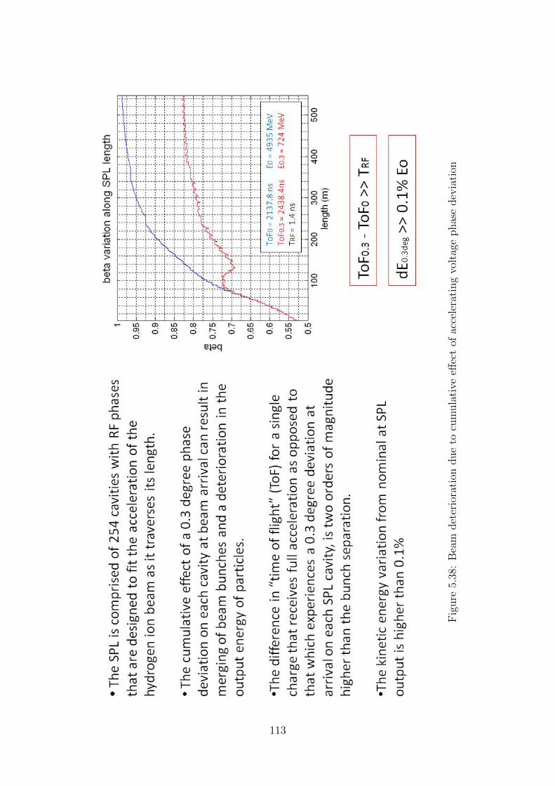
Fig

ure

5.38

:B

eam

det

erio

rati

ondue

tocu

mula

tive

effec

tof

acce

lera

ting

volt

age

phas

edev

iati

on

113

Fig

ure

5.39

:Slo

wfe

ed-f

orw

ard

schem

eusi

ng

smal

lex

cita

tion

114

Fig

ure

5.40

:B

eam

det

erio

rati

onso

luti

on:

random

isin

gcu

mula

tive

phas

eeff

ects

115

5.6 Further Analysis and Stability Considerations

Until this point in the report, we have shown the versatility of the model with regardto the stabilisation of the electric field within superconducting RF resonant cavitieswith the specifications needed to build the SPL. However, no analysis is full withoutpointing out some of the limitations of the system. As shown in the last chapter,a >1.5% difference in the cavities’ quality factor can result in a deviation on cav-ity voltage magnitude that cannot be resolved using feedback or feed-forward whenmore than a single cavity is driven by one Klystron. The feedback loop compensatesthe vector sum of the cavity voltages, keeping it within specifications (0.5% magni-tude and 0.5 phase deviations), but that does not mean that each cavity separatelyis also exhibiting the same behaviour. The cavity voltage magnitudes vary with thedifference in the loaded quality factors and their magnitudes and phases vary withthe difference in their Lorentz detuning coefficients. To observe the extent of thesevariations, a simulation “sweep” was carried out, recording the voltage magnitudedifference at the output, as well as the phase difference (voltage of cavity 1 minusvoltage of cavity 2). For both the loaded quality factor (QL) and Lorentz detuningcoefficient sweeps (K), it was found that fitting a curve based on the results was moresuited than an analytic approach. With this curve, an exhaustive analysis using amodel for the whole SPL length can be developed as a parallel project, to observe ifthe beam cannot ultimately tolerate the single cavity variations even though theiroverall effect (vector sum) might appear within specifications. The results are asfollows:

Cavity voltage difference between two cavities with different loaded qual-ity factors

QL optimal = 1.2078× 106

Measurements of the voltage difference between both cavities were taken with feed-back control on their vector sum. As the quality factor of the cavities has noimpact on their voltage phases, the analysis is restricted to cavity voltage magni-tudes. The sweep was done using values for QL1 and QL2 (for cavities 1 and 2respectively) from 1e6 to 1.5e6 at 1e4 intervals resulting in 51 different values of QL

and 51*51=2601 different QL1, QL2 combinations minus redundant values. Thus,the obtained Vdiff = f(QL1, QL2) curve was fitted using 1326 points. The polyno-mial equation relating the voltage output difference to the individual loaded qualityfactors of the cavities was found to be of the form

Vdiff (x, y) = p00 + p10x+ p01y + p20x2 + p11xy + p02y2 (5.5)

where x = QL1 and y = QL2, with coefficients:

p00 = 1.742× 106

p10 = 34.63p01 = −37.44

116

p20 = −8.286× 10−6

p11 = 1.477× 10−7

p02 = 9.261× 10−6

Figure 5.40 below shows the curve fit. The blue points are given by model experimen-tal results, while the continuous plane is given by the equation above. The individualcavity voltages can be reproduced as Vcav1 = Vacc +

Vdiff2

and Vcav2 = Vacc − Vdiff2

,where the low voltage corresponds to the cavity with lower QL.

Cavity voltage difference between two cavities with different Lorentz de-tuning coefficients

K optimal= 0 Hz/(MV/m)2

As before, measurements were taken in closed-loop operation with no feed-forward.In this case, however, both the cavity voltage magnitude and phase are affected byvarying Lorentz detuning coefficients. Two curves are therefore fitted, with values ofK from -1 Hz/(MV/m)2 to 0 Hz/(MV/m)2 using 0.01 Hz/(MV/m)2 intervals (5151points). Figures 5.41 and 5.42 show the fitted surfaces for magnitude and phasedifference respectively. The respective polynomials for the voltage magnitude andphase difference were found to be:

Vdiff (x, y) = p00 + p10x+ p01y + p20x2 + p11xy + p02y2 (5.6)

with coefficients:

p00 = −8.644p10 = −3.062× 1014

p01 = 2.988× 1014

p20 = −3.061× 1028

p11 = 2.37× 1026

p02 = 3.037× 1028

and:

Vdiff (x, y) = p00 + p10x+ p01y (5.7)

with coefficients:

p00 = 6.801× 10−4

p10 = 3.5× 1012

p01 = −3.498× 1012

where x=K1 and y=K2.

117

Once again, the individual cavity voltage magnitudes can be found using the afore-mentioned formula centered at Vacc. The phase equation is centered at 0.

Figure 5.41: Curve fit for cavity voltage difference with varying loaded quality factor

Figure 5.42: Curve fit for cavity voltage magnitude difference with varying Lorentzforce detuning

All system configurations described are part of an analysis whose goal is to prove theviability of a superconducting, high-power proton LINAC from the point of view of

118

Figure 5.43: Curve fit for cavity voltage phase difference with varying Lorentz forcedetuning

the RF systems. The SPL is not only a challenge because of the energies and bunchdensities involved, but the fact that the underground cavities are driven by pulsedklystrons operating from the surface adds complexity to the situation. The timedelay of the feedback loop becomes an issue when the connectors are of considerablelength, and the operating frequency of the system is of the order of hundreds ofmegahertz. In addition to this effect, pulsed generators introduce transients to thesystem with components in the whole frequency spectrum. A feedback delay of 5us is included in the model, and stability analysis was carried out using low-passfilters to model the feedback loop and generator frequency responses. Finally, theproportional feedback gain was set to ensure that the system is stable [21] [22]. Theopen-loop transfer function is given by:

HSPL(s) = HFB(s)HKly(s)HCav(s)HDelay(s)Hprobe(s) (5.8)

where

HFB(s) =GFBs

2πfcFB+ 1

HKly(s) =GFBs

2πfcKly+ 1

(5.9)

Hprobe(s) = Gprobe HDelay(s) = e−sτ (5.10)

HCav =

[Hs(s) −Hc(s)Hc(s) Hs(s)

](5.11)

The cavity self and cross-coupled transfer functions are given by

119

Hs(s) = σR

[s+ σ

(1− ∆ω

ωR

)(s+ σ)2 + (∆ω)2

]

Hc(s) =σ2R

ωR

[s+

(σ + ωR∆ω

σ

)(s+ σ)2 + (∆ω)2

] (5.12)

whereσ =

ωR2QL

ωR is the resonant frequency of the cavity, and ∆ω = ωR − ω0 is the frequencydeviation between RF source and resonant frequency of the system. The value waschosen as the maximum value observed in simulations.

We find that the problem of observing the characteristics of the system transferfunction is not as straightforward as expected, as the behaviour of the model is theresult of a coupled action between in-phase and quadrature signal components. Theoutput of the system can be expressed using the following coupled equations:

YI(s) = HK(s)Hs(s)XI(s)−HK(s)Hc(s)XQ(s)

YQ(s) = HK(s)Hs(s)XQ(s) +HK(s)Hc(s)XI(s)(5.13)

whereHK(s) = HFB(s)HKly(s)(s)HDelay(s)Hprobe(s)

I/Q refer to inphase and quadrature components, and s/c refer to the self and cross-coupled components of the cavity transfer function respectively. X and Y are inputsand outputs to the system. If we assume a purely inphase unit step input to thesystem to begin with, the system equations simplify to yield

YI(s) = HK(s)Hs(s)XI(s)

YQ(s) = HK(s)Hc(s)XI(s)(5.14)

and so we can investigate the stability behaviour of the system by analyzing thetransfer function given by

HK(s)(Hs(s) + iHc(s)

)in both magnitude and phase.We want to find GFB such that the open-loop transfer function is such that theclosed-loop system is stable. For a feedback loop with a 100 kHz bandwidth and a1 MHz bandwidth klystron driving an SPL cavity at its resonant frequency of 704.4MHz, we find a gain margin of about 43 dB (x150) as shown in figure 5.43.

120

Fig

ure

5.44

:B

ode

plo

tof

open

-loop

syst

em

121

Chapter 6

Conclusion and Outlook

Through the course of this report, a detailed analysis of a model for controlling thebeam acceleration along the superconducting proton linear accelerator has been de-scribed. The system consists of 254 accelerating structures with individual controlloops ensuring rigorous beam specifications in terms of output energy and time-structure. At its most restrictive of configurations, the SPL low speed section willconsist of 54 β = 0.65 resonant cavities accelerating a 40 mA beam with a time-structure of 0.4 ms pulses repeating every 20 ms with an accelerating field strengthclose to 19 MV/m, while the high speed 200 β = 1 cavities will reach electric fieldsof 25 MV/m. The challenges arise from the fast-pulsing H− source and the highfields within the thin walled niobium cavities, where Lorentz force effects induce adeformation in shape, resulting in a detuning in resonant frequency. The controlfor the low-speed section includes dedicated RF loops acting on a single klystronper cavity scheme whereas the high-speed section favours a 2 cavity per klystronconfiguration with control loops acting on the vector average of the cavity voltagesin terms of magnitude and phase. This gives rise to problems in dealing with slightlymismatched cavities in terms of Lorentz detuning factor and loaded quality factors.A piezo-electric system is in place to oppose the effects of Lorentz deformationsand full SPL simulation reveal a best case of just under 10% loaded quality factormismatch between adjacent cavities from ideal value. Fast RF feedback and slowfeed-forward are intended for compensating synchronous angle effects and cumula-tive phase errors, as well as other non-foreseeable or uncharacterised errors.From the RF control point of view, there is strong evidence to support the devel-opment of an I/Q system that can be successful in dealing with the foreseeabledrawbacks that arise when attempting an engineering feat of this magnitude.

122

Bibliography

[1] R. Garoby et al., “Project Periodic Report,” tech. rep., sLHC-PP Project,CERN, Geneva, Switzerland, May 2010.

[2] J. Le Duff, “High Frequency Non-Ferrite Cavities,” in Cern AcceleratorSchool Proceedings, Seeheim, Germany, May 2000. Edited by J. Miles, CERN-2005-003, p. 47.

[3] T. Weiland, M. Krasilnikov, R. Schuhmann, A. Skarlatos, and M. Wilke,“Review of Theory (I, II, III),” in Cern Accelerator School Proceedings,Seeheim, Germany, May 2000. Edited by J. Miles, CERN-2005-003, p. 1.

[4] T. Schilcher, Vector Sum Control of Pulsed Accelerating Fields inLorentz Force Detuned Superconducting Cavities. PhD thesis, HamburgUniversity, Hamburg, Germany, April 1998. TESLA-98-20.

[5] J. Tuckmantel, “Cavity-Beam-Transmitter Interaction Formula Collec-tion with Derivation.” Internal Note, CERN-ATS-NOTE-2011-002 TECH.

[6] P. B. Wilson, “Transient Beam Loading In Electron - Positron StorageRings,” Preprint, CERN-ISR-TH-78-23-rev.

[7] D. Boussard, “Beam Loading,” Preprint, CERN-SPS-86-10-ARF.

[8] F. Gerigk, “SPL Web.” https://twiki.cern.ch/twiki/bin/view/SPL/

SplWeb.

[9] F. Gerigk, “SPL parameter table.” https://twiki.cern.ch/twiki/bin/

view/SPL/SPLparameterList.

[10] W. Hofle, “SPL LLRF Simulations Feasibility and Constraints forOperation with more than one Cavity per Klystron Power Over-head,” in 3rd SPL Collaboration Meeting, Geneva, Switzerland, Novem-ber 2009. https://indico.cern.ch/materialDisplay.py?contribId=

80&sessionId=11&materialId=slides&confId=63935.

[11] M. Luong and O. Piquet, “RF Control System Modeling,” in IP-EUROTRANS / DM1 / WP1.3, June 2007.

[12] “PID controller.” http://en.wikipedia.org/wiki/PID_controller.

123

[13] K. J. Astrom and R. M. Murray, Feedback Systems. (Princeton UniversityPress, New Jersey, Oxfordshire, 2008), Electronic Edition Version 2.10c, Chap.10. http://www.cds.caltech.edu/~murray/amwiki.

[14] C. Brosilow and B. Joseph, Techniques of Model-Based Control. (PrenticeHall, New Jersey 2002), Chap. 9. www.bgu.ac.il/chem_eng/pages/Courses/oren%20courses/Chapter_9.pdf.

[15] M. Hoffman, “Digital Signal Processing Mathematics,” in Cern Accelera-tor School Proceedings, Sigtuna, Sweden, May-June 2007. Edited by D. Brandt,CERN-2008-003, p. 10.

[16] P. S. Maybeck, Stochastic Models, Estimation, and Control. (AcademicPress, New York, San Francisco, London, 1979), Vol.1, Chap. 1.

[17] P. S. Maybeck, Stochastic Models, Estimation, and Control. (AcademicPress, New York, San Francisco, London 1979), Vol.1, Chap. 3.

[18] G. Welch and G. Bishop, “An Introduction to The Kalman Filter,” tech.rep., TR 95-041, University of North Carolina at Chapel Hill, Department ofComputer Science, Chapel Hill, NC, USA, July 2006.

[19] J. Holma, “The Model and Simulations of the LHC 400 MHz CavityController,” Internal Note, CERN-AB-Note-2007-012.

[20] P. A. Posocco, “Longitudinal Error Studies Description.” CERN, Geneva,2011 (unpublished).

[21] R. Garoby, “Low-Level RF and Feedback,” in Joint US-CERN-Japan Ac-celerator School on Frontiers of Accelerator Technology Proceedings, Tsukuba,Japan, September 1996. Edited by S. Kurokawa, M. Month, and S. Turner, p.455, Article CERN-PS-97-034-RF.

[22] W. Hofle, “Cavity-Laplace.” CERN, Geneva, 2009 (unpublished).

124