progress in nodal methods for the solution …li.mit.edu/stuff/cnse/paper/lawrence86pne.pdf · 272...

Prooress in Nuclear Energy, Vol. 17, No. 3, pp. 271-301, 1986. 0149-1970/86 $0.00+.50 Printed in Great Britain. 1986 Pergamon Journals Ltd.

PROGRESS IN NODAL METHODS FOR THE SOLUTION OF THE NEUTRON DIFFUSION AND TRANSPORT EQUATIONS

R. D. LAWRENCE*

Applied Physics Division, Argonne National Laboratory, Argonne, Illinois 60439, U.S.A.

(Received 21 October 1985)

Abstract--Recent progress in the development of coarse-mesh nodal methods for the numerical solution of the neutron diffusion and transport equations is reviewed. In contrast with earlier nodal simulators, more recent nodal diffusion methods are characterized by the systematic derivation of spatial coupling relationships that are entirely consistent with the multigroup diffusion equation. These relationships most often are derived by developing approximations to the one-dimensional equations obtained by integrating the multidimensional diffusion equation over directions transverse to each coordinate axis. Both polynomial and analytic approaches to the solution of the transverse-integrated equations are discussed, and the Cartesian-geometry polynomial approach is derived in a manner which motivates the extension of this formulation to the solution of the diffusion equation in hexagonal geometry. Iterative procedures developed for the solution of the nodal equations are discussed briefly, and numerical comparisons for representative three-dimensional benchmark problems are given.

The application of similar ideas to the neutron transport equation has led to the development of coarse-mesh transport schemes that combine nodal spatial approximations with angular representations based on either the standard discrete-ordinate approximation or double P, expansions of the angular dependence of the fluxes on the surfaces of the nodes. The former methods yield improved difference approximations to the multidimensional discrete-ordinates equations, while the latter approach leads to equations similar to those obtained in interface- current nodal-diffusion formulations. The relative efliciencies of these two approaches are discussed, and directions for future work are indicated.

1. INTRODUCTION

It has been nearly 30 years since the initial implemen- tation of finite-difference techniques in computer codes designed to solve the few-group neutron diffusion equations in more than one spatial dimension. Codes such as the PDQ program 1 developed at Bettis Atomic Power Laboratory employed very novel iterative acceleration techniques, and their development represented a major advance in our capability to analyze nuclear reactors. Further improvements in solution algorithms, combined with continued advances in computer hardware, have made possible the solution of increasingly complicated problems in reactor physics. However, even with current computers, practical limitations on computer storage and execution time generally prohibit the explicit modeling of each fuel pin in a light water reactor (LWR). Instead, 'equivalent' few-group diffusion-theory parameters 2 are determined for relatively large homogeneous regions often consisting of entire fuel assemblies in the radial plane. With these parameters in hand, global solutions are computed for this homogenized-assem-

* Present address: Schlumberger-Doll Research, Old Quarry Road, Ridgefield, CT 06877-4108, U.S.A.

bly representation of the reactor. Solution of this problem using traditional finite-difference techniques requires a large number of mesh points in order to represent accurately the spatial variation of the neutron flux. The computational expense associated with these calculations motivated the early development of less rigorous, yet more computationally efficient techniques oriented towards the determination of the flux averaged over each homogeneous region or 'node'. This class of methods thus became known as nodal methods, and the FLARE model 3 developed in 1964 is representative of the first generation of these schemes.

The evolution of nodal methods over the 20 years since the development of the FLARE method has proceeded along two rather different paths. The first direction has focused on refinements to the initial one- group FLARE model, which involved parameters adjusted to match actual operating data or the results of more accurate calculations. A number of improved schemes have resulted from this work, and these methods, often referred to as 'simulators', are the subject of a review paper 4 which appeared in this Journal several years ago. (The reader is also referred to earlier review papers by Henry 5 and Wagner. 6) FLARE and its successors have been used extensively

271

272 R.D. LAWRENCE

by utilities and vendors in the analysis of LWR's, and with appropriate tuning of adjustable parameters, these models are capable of accurate predictions of conditions in an operating reactor. Most of these methods are,based on so-called 1.5 group theory 4 and most treat LWR reflectors using albedos computed from the results of auxiliary calculations or analytical procedures. As a consequence, in the limit of infinitely fine spatial mesh, these schemes do not yield solutions consistent with the exact solution of the few-group diffusion equation. This behavior, plus more practical concerns about the use of simplifying assumptions and adjustable parameters under different (e.g. transient) conditions, has led to the development over the past 10 years of an alternate class of nodal schemes. Some- times referred to as 'consistently formulated '6 or 'modern' 7 nodal methods, these schemes avoid the use of empirical parameters by computing inter-node coupling relationships using higher-order approximations to the multigroup diffusion equation. Therefore, unlike the earlier nodal simulators, these more recent nodal schemes can be viewed as true coarse-mesh approximations to the neutron diffusion equation, and thus can be expected to converge to the exact solution of the diffusion equation in the limit of zero mesh spacings. It is these consistently formulated nodal methods with which we will be concerned in this review paper.

As noted above, the use of nodal methods for global LWR calculations requires the determination of 'equivalent' parameters for each assembly. These homogenized parameters traditionally have been computed by weighting the spatially-dependent cross sections with the flux solution obtained in an assembly calculation with zero net current boundary conditions. Recent nodal schemes yield very accurate approximations to the diffusion equation, and the errors introduced by the use of flux-weighted cross sections may be much larger than the spatial truncation errors present in the nodal solution of the homogenized problem. Therefore, the development of accurate homogenization procedures is essential to the successful application of nodal diffusion methods to LWR analysis. This important aspect of nodal analysis is reviewed in a companion paper by Smith. s

In Section 2 of this paper, we review recent work in the development of nodal diffusion methods for global calculations, and indicate briefly how these methods are modified to accommodate recent advances in homogenization procedures. Both polynomial and analytic nodal formulations in Cartesian geometry are discussed, and the Cartesian-geometry polynomial method is derived in a manner which motivates the extension of this formulation to the solution of the

diffusion equation in hexagonal geometry. The high computational efficiency demonstrated for the consistently formulated nodal diffusion methods has prompted the application of analogous ideas to the numerical solution of the neutron transport equation, and two nodal transport formulations are discussed in Section 3. The first combines nodal spatial approximations with the conventional discrete-ordinates angular discretization, while the second uses double Pn expansions of the angular dependence of the nodal interface fluxes. The latter formulation is shown to yield interface current equations very similar to those obtained in the nodal diffusion methods.

2. NODAL METHODS FOR THE SOLUTION OF THE DIFFUSION EQUATION

2.1. Introduction

We begin with the multigroup neutron diffusion equation written in P1 form:

V ' Jg(r) + Y~(r)~g(r) = Qg(r), re v, (1)

J g ( r ) = - Dg(r)V~g(r), (2)

where

1 ~

ag(r)=~g~,=l ~gv~aY'(r)~b¢(r)+g,~l ~ 3z~g,(r)~¢(r), (3)

g'~g

2 denotes an eigenvalue, and the remaining notation is standard. 2 Equations (1) and (2) are solved subject to the conditions that the neutron flux ~bg(r) and the surface-normal component of the net current Jg(r) be continuous across all material interfaces contained with the reactor. Appropriate boundary conditions are imposed on all external surfaces.

Nodal procedures are based on subdividing the domain V into nodes V k, k = l , . . . , K , such that wV k= V and vkc~vZ=O, k:/:l, and then integrating equation (1) over an arbitrary node. Let us assume for the moment that homogenized cross sections are available for each node. As mentioned above, such parameters are often obtained by weighting the spatially-dependent cross sections with the flux obtained in a local calculation with zero net current conditions on the boundaries of the assembly. Inte- grating equation (1) over re V k, dividing by the node volume V k, and then applying the divergence theorem to the integrated leakage term yields the balance condition

- - n Jg(r,) + Y~o q~0- Qa, (4) vk d 2r~ ~ • ,.k k_ --k sgS k

Nodal diffusion and transport methods 273

where c~k o is the node-averaged flux,

~ko--V 1~ t ~d3r~bko(r)' dr tV

0~ is the node-averaged group source term, and ~,k denotes the value of the removal cross section averaged over V k. Apart from the determination of the homogenized cross sections, equation (4) is an exact balance equation; however, the solution of this equation requires additional equations relating the surface-averaged net current on each surface of the node to the fluxes in the two nodes on either side of the surface. It is these additional coupling relationships that characterize the various nodal schemes which have been developed for the solution of the neutron diffusion equation. Certainly one of the simplest means of obtaining these relationships is the approach used to derive the standard mesh-centered finite difference equations, in which the surface net currents are approximated by assuming that the flux varies linearly between the node centerpoint and the midpoint of any surface of the node. Eliminating the surface fluxes by enforcing continuity of net current and flux across each interface leads to equations involving only the node-averaged fluxes. Of course, the development of nodal schemes is motivated by the need for improved accuracy relative to the finite- difference method, and alternative procedures for deriving the coupling relationships in Cartesian and hexagonal geometries are discussed in the following sub-sections.

Before proceeding further, however, it is necessary to add several comments concerning the solution of equation (4) in light of recent advances in the development of homogenization procedures. Let us assume that we know the solution to equations (1) and (2) for the heterogeneous model of the reactor, and then use this reference solution to compute homogenized cross sections and diffusion coefficients (which can be directionally dependent). Irrespective of the manner in which the homogenized cross sections are determined, the solution of equation (4) using these homogenized values cannot reproduce the node-averaged reaction rates and leakages inferred from the reference solution without the introduction of additional degrees of freedom. This shortcoming has led to the development of more rigorous homogenization procedures based on 'equivalence theory', a concept introduced by Koebke 9.1o and subsequently generalized by Smith. l 1,12 Koebke demonstrated that it is possible to develop a homogenization method which is capable of reproducing rigorously all node-integrated properties (i.e. reaction and leakage rates) of the known reference heterogeneous solution. Equivalence theory requires

the introduction of additional degrees of freedom into the solution of the homogenized balance equation, equation (4), and the manner in which these parameters are introduced is the essential difference between Koebke's and Smith's formulations. This and other differences in the two developments are discussed in Refs 8 and 12, and for our purposes here, we simply note that both formulations require that the method developed for the solution of equation (4) permit the surface-averaged fluxes to be discontinuous across each nodal surface. This is accomplished in generalized equivalence theory 11'az by introducing additional homogenization parameters called 'discontinuity factors', which are defined by

t ~ h e t , k l k l _ TO

f0 -- (5) ~ h o r a , k l " T g

Here, kl denotes the surface common to nodes k and l, t~h,t.k~ is the surface-averaged flux obtained from the 0 reference heterogeneous solution, and ,~hom,U is the "r 0

surface-averaged flux implied by the solution to equation (4) for the k th node. Since the face-averaged heterogeneous flux must be continuous across an interface, equation (5) implies the following interface condition on the homogenized flux (which we write without the identifying superscript):

funk, =flk3tk (6) g T 0 a g ~ O "

Note that if the discontinuity factors are unity, equation (6) reduces to the usual flux-continuity condition. Of course, in practice the reference heterogeneous solution is not known, and the determination of the homogenization parameters (including the discontinuity factors) for practical situations is discussed in Refs 8-15. Therefore, in the following sub- sections, we will be concerned with approximations based on equations (4) and (6) with known values of the homogenization parameters.

2.2. Cartesian geometry Equation (1) takes the form

~xg- Jk°~ (x, y, z) + ~YO Joy Y, z) + ~Z j~(x, y, z )

,.k k z), (x, z)~ VL + x 0 q~0(x, y, z) = Q~(x, y, y, (7)

where, for example, the x-component of the net current is

k C3 k Jkx(x, y, z)= --D o t~x(%(x, y, z), (8)

and cross sections are assumed to be independent of

274 R.D. LAWRENCE

position within the node. It is convenient to take the center of the node as the origin in local coordinates, and define the k th node in terms of the mesh spacings:

vk: (X, y, Z) x e [ - - A x ' / 2 , +Ax' /2] , ye[- -Ayk/2

+ Ay k/2], Z e [ -- Az k/2, + Az'/2].

The node volume is given by the product of the mesh spacings, and in the following development we omit the node index on the mesh spacings. We use x + and x - to denote the plus-x-directed (right) and minus-x- directed (left) faces of the node, with similar notation for the y- and z-directed surfaces. Using this notation, the balance equation [equation (4)] is

t t , _ _ k k - - OY- ] Ax [J;x+ - J ; ~ - ] + ~yy [J;r+ j k

t r,k k__ --k + Azz [s;'~÷ - jko,_ ] + Y', ~o - Qo, (9)

where

, 1 I Az/2 (" Ay/2

c~°=Ax Xy Az d_,x,/2dz J_ar/2dY

f ax~2 -ax/£ dx ~bk(x, y, z), (t0)

and, for example, ark+ are the x-components of the net current averaged over the x-directed faces of the node:

t /. A~/2 f Ay/2 j~k± _ Ay Az 3 [_Az/2 dz / dy

, J - Ay/2

- o ~ ¢ : ¢ x , y, zL~ ±~/~. (t t)

All face-averaged currents and fluxes with node index k are evaluated in the limit as the node surface is approached from within the k th node. Surface-aver-

/'out,k~ and incoming (e.g. o0~+, aged outgoing (e.g. ~0~+, lin'k ~ partial currents are defined in an analgous manner, and the partial currents satisfy the usual relationships

jff:tik_j~,~ =ark+ (12a)

j ~ t , k _ j ~ , k = _ jkx_ (t2b)

2rro-t.k .a_ fi., , 1 - .~' (t 2c) L~OX± " ° g x ± J - - W ' O x ± ,

where ok0x ± denotes the face-averaged fluxes. Note that the balance condition, equation (9), can be written in terms of surface-averaged partial currents using equations (12a) and (12b).

2.2.1. The transverse-inteoration procedure. As noted in Section 2.1, it is the equations used to compute the surface currents in equation (9) which

distinguish one nodal formulation from another. However, nearly all recent nodal methods have one feature in common, and that is they are based on approximations to one-dimensional equations derived by integrating the three-dimensional equation over the two directions transverse to each coordinate axis. For example, operating on equations (7) and (8) with

1 (. Az/2 ( ' Ay/2

dz Ay Az J_a~/z J_, dy, yields the one-dimensional P - 1 form of the x- direction equation:

d ~ r,k k _ 1 L~r(x) dx :;x(x) + X, ,~o,,(x)- O.*ox(x) - Ay

1 - A-~ L ~ (x), (13a)

~xix)= - O ' d ~x(x), (tab) o dx

where f' Ayl2

d-az/2 J-ar/2 Y'

(14)

and the leakages transverse to the x-direction are defined by

Az d-a~12

(15a)

1 I Ay/2 k O ~l z=az/2 L k°z(x) ~-- Ayy ,J - a~,/2 d y - D o ~z $~(x, y, zm= - a~/2 .

(t5b)

Substitution of equation(13b) into equation (13a) yields the conventional second-order form of the transverse-integrated equations:

d , d , r ,k k

dx Do dxx ~°x(x) + x° q~'x(x)

1 1 L~, (x). (16) = ~?~(x) - yy L;, (x) - Az

The one-dimensional fluxes and transverse leakages are related to their respective node-averaged values by

t Ax/2 k k Ax .J-a~/2 dx q~o~(x) = ~ (17a)

1 [ Ax[2 - - dx Effy(x)= - ' - k _ j k Loy-d~r+ or- (17b) Ax d -~ /2


1 r A x / 2 r-k __ F-k - - k - - I d x L g ~ ( x ) = L g z - ~ = + - J ~ = _ . (17c) A x d - ~ x / 2

Integrating equation (13a) over x, dividing by Ax, and using equations (17) yields the nodal balance equation, equation (9). One-dimensional equations in the y- and z-directions are derived in an analogous manner.

The development of nodal schemes based on the approximation of equation (16) is motivated by the simple observation that it is generally easier to solve a one-dimensional equation than a two- or three- dimensional equation. Of course, in order to solve equation (16) it is necessary to have some knowledge of the shape of the transverse-leakage terms. As noted in Section l, nodal methods traditionally have been oriented towards the calculation of the node-averaged fluxes (and leakages), and equation (16) provides a convenient framework for the development of schemes with this objective. An important consequence of this approach is that the one-dimensional solutions contain only information concerning the shape of the one- dimensional fluxes, and it generally is not possible to reconstruct rigorously the multidimensional flux shape within the node using only the information from the solution of equation (16) and its y- and z-direction analogs. However, flux-reconstruction techniques ~6 based on the use of higher-order polynomial fits to the information obtained from the nodal calculation have been developed, and numerical tests 16 have shown that the reconstructed flux shapes agree well with fine- mesh finite-difference calculations. It should be noted that ultimately it is the flux shape in the heterogeneous node that is required, and this information can be obtained by modulating the solution computed in a local assembly calculation with a 'form function' representing the reconstructed flux in the homogeneous node. These procedures are described in Refs 13-16, and will not be discussed further here, other than to note that these procedures have made possible the accurate calculation of pin-power distributions in a LWR using the nodal methods discussed in this paper.

The use of solutions for one-dimensional problems to construct multidimensional nodal solutions appears to have originated with the development in the early 1970's of two very different nodal formulations, the Nodal Synthesis Method 1 v (NSM) of Wagner, and an analytical procedure S'~8 due to Antonopoulous and Henry. Both methods approximated the transverse-leakage terms using bucklings computed under the assumption that the flux within the node is separable into a normalized product of one-dimensional fluxes. Like the much earlier Gross-Coupling

Method, 19 the NSM used coupling coefficients defined by ratios of face-averaged partial currents to node- averaged fluxes, e.g.

~.x+ -= ~ x ~ .

Using these expressions to eliminate the surface currents in equation (9) yields a finite-difference-like equation for the nodal flux. The coupling coefficients in the NSM were evaluated from the results of one- dimensional finite-difference calculations for each one- dimensional 'channel' in the reactor, and these coefficients were recomputed periodically during the iterative solution of the nodal equations. The analytic procedure ~'ls did not involve any auxiliary calculations, but instead used truncated Taylor-series expansions of exact analytic expressions (for one energy group) relating the face-averaged net current to the average fluxes in the two nodes on either side of the surface. These expressions depend upon the global eigenvalue and the transverse bucklings, and hence it was necessary to update the coupling expressions during the iterative procedure.

The NSM and the one-group analytic method represented important steps in the development of nodal schemes with more consistent, more computationally-efficient procedures for the determination of the inter-node coupling relationships. The desire to eliminate the fine-mesh finite-difference calculations in the NSM led to the development of the well-known Nodal Expansion Method, Z 0-23 in which polynomials defined within each node are used to approximate the one-dimensional fluxes defined in equation (14). The analytic procedure has been extended to two groups, 24.25 and further refinements resulted in the very efficient Analytical Nodal Method 26'27 implemented in the QUANDRY code. The essential difference in the polynomial and analytic approaches suggests classification of the methods developed for the solution of equation (16) on the basis of whether information obtained from an analytic solution of the diffusion equation within the node is incorporated into the numerical scheme. In the first class, we include schemes in which the one-dimensional fluxes are approximated by a polynomial without the use of analytic information. Examples of the polynomial methods are the aforementioned Nodal Expansion Method, 20 23 the polynomial scheme 28'2~ developed by Sims, the NODLEG method 29 due to Maeder, and a polynomial method 3° developed for multigroup fast-reactor analysis. Examples of the second class, the analytic methods, are the Analytical Nodal Method, 2,-27 the Nodal Green's Function

276 R.D. LAWRENCE

Method 3~'a2 and the AN2D method. 33 The polynomial and analytic nodal methods are described in the following sub-sections.

2.2.2. The polynomial methods. The one-dimensional fluxes are approximated by polynomials of the general form

N

k ~ k a;xnfn(x) , Gx(X)= ~do(x)+ Y, n = l

x e [ - Ax/2, + Ax/2], N_> 2, (18)

where, in accordance with equation (17a), the basis functions satisfy

± lax,2 d x f . ( x ) = { l o n=O (19) Ax d_ax/2 n = 1 . . . . . N.

The node-averaged flux satisfies the balance condition, equation (9), and the choice of basis functions and the determination of the expansion coefficients ag~,k characterize the various methods. One feature common to the polynomial schemes discussed here is that in addition to the node-averaged flux, the principle unknowns are the face-averaged partial currents across the nodal interfaces. Equations for the partial currents can be derived by inserting equation (18) into Fick's law [equation (13b)] evaluated on the node surfaces. These interface current equations are solved in conjunction with the node balance equations.

As an example, we consider the earliest of the polynomial methods, the Nodal Expansion Method 20-23 (NEM). In the following development, the NEM approximations 22 are cast in a form 3° which parallels the application in Section 2.3 of similar ideas to the solution of the diffusion equation in hexagonal geometry. The basis functions are

fo(x) = 1 (20a)

X

f , ( x ) =- A x - ~ (20b)

f2(x) -- 3¢ 2 --¼ (20c)

f 3 ( x ) ~ ¢ ( ~ - - ½ ) (¢ + ½ ) (20d)

f,)()x = (~z _ ~oo) ({: -- ½) (~ + ½), (20e)

and so on. The NEM polynomial is constructed such that the two face-averaged fluxes in the x-direction are preserved, i.e.

k - - k ~g~( + Ax/2)= 05g~ ±.

These constraints are satisfied by setting k k k ag~l = 05,~+ - q~g~_ (21a)

akx2 k k = 05ox+ +050:, - - 2qSok, (21b)

and requiring that the higher-order basis functions satisfy the additional constraints:

f~( +_ Ax/2) = O, n = 3 . . . . . N.

Equations for the outgoing partial currents on the two x-directed surfaces of the node are readily obtained:

out,k k d J ~ + = - Do ifi~gx(X)]~ = a~/2 + J ~

Dk I 1 k , 1 k ] . - - i n k o k + ~ a o x 4 l + j d x T " = - Ax a°~l + 3ag~2 + 2 ag~3

L (22a)

j~7,.k= + D ~ d k in* dx (b gx(X)[" = - A:,/2 + J3~,'-

D k [ k I k l_k ] , . i , , k +AXXL aox' -3%~2 + 2agx3--5"gx4J -r'lgx~"

(22b)

Using equations (21) and (12c) to eliminate %xk 1 and in favor of the partial currents and node-averaged aox2

flux yields two coupled equations for the outgoing partial currents in terms of the node-averaged flux, the incoming partial currents on the x-directed surfaces, and the higher-order expansion coefficients. If, for the

k _ k =0 [i.e. N = 2 in moment, we assume aax 3 =aax 4 equation (18)], then equations (22), their y- and z- direction analogs, and the nodal balance equation represent a total of seven equations for the seven unknowns (the node-averaged flux and the six outgoing partial currents) per node. Since the incoming partial currents are simply outgoing partial currents from adjacent nodes, and the node source terms Okg are computed in terms of the node-averaged fluxes, this system of equations is well-posed. As will be discussed in Section 2.4, a slightly modified interface condition is required if the interface fluxes are discontinuous as in equation (6).

For N > 2 in equation (18), the higher-order coeffi- k , n>3, are determined by applying a cients aax n

weighted residual procedure to equation (13a). Mul- tiplying equation (13a) by weight function w,(x), n = O, . . . . N - 2 , and then integrating over x e [ - A x / 2 , + Ax/2] yields the moment equation

d _ 53. k k (w.(x) , {ix ~ , ( x ) ) + o" 050:'~

_ k 1 k 1 - Qgx. - Ay Lgyx" Az L°R~"' (23)

where the inner products are

J [" Ax/2

- A~ J-a~/2 dx w.(x)~Jko~(x) -- 05~.,

(24a)


<w,Cx), L~y(x)> - L+ky~,,, (24b)

k and the spatial moments Q k and L~,x, are defined in an analogous manner. The nodal balance equation is recovered using Wo(X ) - 1 and noting that ~bkg~o--~kg. Equations for the coefficients aox at' and a0~ak are obtained by weighting with w~(x) and w2(x ), where these functions are specified using either moments weighting 22,

%(x)=fl(x) (25a)

w2(x ) =fE(x), (25b)

or Galerkin weighting 2z,

wl(x)-f3(x ) (26a)

w2(x ) -f+(x). (26b)

Numerical studies 22 have shown that moments weighting yields superior accuracy relative to Galerkin weighting. Integrating the first term in equation (23) by parts, and then using equations (25) yields the following moment equations:

1 1 ~ + 1 DR k _l_]~r.kt~k 2Ax Ax Ax ao,a - + ",'oxt

1 k 1 k (27a) = ook.+, - a y - L , , = ,

1 1 Z~o~+ 3 D~ k ~_,r,.k,6t 2 Ax Axx Axx %x2 - -0 "ro~z

1 k 1 = o o k 2 - - Ayy L°r"2 AZ Lokzx2 (278)

where

~x -- J~x + + j k _ (28a)

~+ - J~x + -J~x_. (28b)

Substituting equations(18) and (25) into equation (24a) yields the following relationships between the higher-order expansion coefficients and the flux moments appearing in equations (27):

rents or flux moments, and then eliminating the flux moments (including the node-averaged flux) in favor of the source and higher-order leakage moments using the balance condition [equation (9)] and the moments equations [equations (27)]. The node-averaged leakages are eliminated in terms of the partial currents. Combining these results with the analogous equations in the y- and z-directions yields an interface current equation of the form

out,k - - k k k k in,k Jg - [ P g ] {Qa-L~}+[Rg]J9 ,

k = 1 . . . . . K; ,q = 1 . . . . . G, (30)

where

j o u t , k _ out,k /out ,k / ou t& /out ,k iou t ,k ./out,kq g =c°l[Jgx+'-ax- '~gy+ '~gr- ' ~ + '-g~

a ~ , k =. col[Jign.k+, j~xn~, j ~ y ~ , j ~ y ~ , j~n~k, j~n,_k ]

= )~o~Z¢ d~g + E (31) 2 2 f , k k ~',$,k~l~k ~ gg,-C'g,, 9'=1 g ' = l

g'~g

k _ k k r~k .hk ~ k k ~ = c o l [ ~ , ~

and

k k k k Egg--col[0, Lgk, , Lgky,, Lo~ , , Lox z , L,y 2 , Lg~2 3.

The components of the leakage vector L k involve sums of the higher-order transverse leakage moments, e.g.

1 k 1 k L,\. = ~ L~,~. + ~ L~=..

The matrices [P~] and [R~] contain nodal coupling coefficients which can be computed and stored for unique nodes characterized by mesh spacings and material zone assignment. Equation (30) is solved in combination with the balance equation and the equations for the flux moments.

The calculation of the transverse-leakage moments requires additional approximations to L~y(x) and L~(x) defined in equations (15). In the initial NEM development 2o, it was assumed that the transverse leakage and the one-dimensional fluxes have the same shape, i.e.

agxak = -- 120~bkxl + 10akxt (29a)

k k k %x4 = - 700~bgxz + 35%x2. (29b)

Equations (27) and (29), plus their y- and z-direction analogs, provide the additional equations required for the calculation of the higher-order expansion coefficients.

The final form of the partial current equations is obtained by first eliminating from equations (22) all expansion coefficients in favor of either partial cur-

1 1 _ _ k ~ 2 k k Ay Lky(x) + Azz La~(x)= [DB ]gx~gx(x). (32)

The bucklings are assumed constant within the node, and are determined by integrating equation (32) over xe [ - Ax/2, + Ax/2] to yield

[DB2"]~x=~o[-~y~Lgr + ~1 L-~o:]. (33)

This approximation is exact if the flux within the node

278 R.D. LAWRENCE

is separable, and it provides a simple means of relating the leakage moments to the flux moments:

1 k 1 k _ 2 k k L°~" ==-Ay L"'x" + Azz L ° ' x " - [ D B ],x~b,~,. (34)

Use of the buckling approximation leads to large errors in many realistic (highly nonseparable) problems, and thus an improved procedure 11 was developed in which the leakage is approximated by a quadratic polynomial, e.g.

k ~ k L,y(x) = p,y(x), xe V k, (35)

where

k - - r--k k k pgr(x) = Lgy + Poylfl(x) + pgy2f2(x), (36)

and fl(x) and f2(x) are defined in equations (20). The expansion coefficients are determined by assuming that pkoy(x ) extends over the k th node and its two immediate x-direction neighboring nodes (denoted by k + and k - ) , and then requiring that the polynomial, upon separate integration (using coordinates relative to the k th node) over x g V k+ and x e V k-, return the two average leakages qy+ and q T ' As indicated in equation (35), p~y(x) is used only to approximate the leakage in the k'h node, even though the coefficients are computed under the assumption that the poly-

.0 nomlal extends over the neighboring nodes as well. Substitution of equation(35) into equation(24b) makes it possible to evaluate the required leakage moments in terms of average leakages (and thus the face-averaged partial currents) in the adjacent nodes. The quadratic leakage fit has little theoretical basis because its derivation does not rely on the diffusion equation itself. Nevertheless, this approximation is used in nearly all recent nodal m e t h o d s 2°-23"25-32

because it produces acceptable accuracy with relative computational simplicity compared to more rigorous procedures (suggested in Ref. 7) based on solving additional equations for the spatial moments of the surface net currents. More recently, a somewhat modified p r o c e d u r e 22'23 has been implemented in the NEM in which flux and current continuity arguments are used to determine the quadratic coefficients. An informative numerical study of the errors associated with the use of the quadratic leakage fit is described in Refs 26 and 27.

Setting the leakage coefficients in equation (36) to zero yields a simple constant (or 'flat') approximation 24,25 to the transverse leakages:

k ~ r-'k Lor(x)=Lgy. (37)

Use of this approximation causes the leakage moments to vanish because the weight functions [equations (25) or (26)] are orthogonal to fo(X)= 1. As noted by

Maeder, 29 the polynomial approximations to the one-dimensional fluxes are then completely consistent with the multidimensional expansion

N N

Skg(x, y, z)= ~ + ~ a~x . f~(x) + ~ a~y. f.(y) n = l n = l

N

+ ~ a;z.f~(z). (38) n = l

A more general expansion 22 (including cross terms) has also been considered, and the quadratic leakage fit can, in principle, be viewed 22 as a means of computing additional cross terms in the general expansion.

The above derivation assumes spatially uniform cross sections within each node, and this basic formulation has been extended in Ref. 23 to include low-order polynomial representations of the spatial dependence of the cross sections within the node. This extension has been s h o w n 23 to be important for the accurate modeling of effects associated with space- dependent burnup and nonlinear feedback.

The polynomial nodal methods due to Sims 25'2s

and Maeder 29 also lead to interface current equations of the same form as equation (30). In Sim's method, the basis functions in equation (18) (with N = 4) are chosen such that the expansion coefficients aox .k , n = 1, . . . ,4, can be identified as J;~:*, j;~,_.k, j~.~ and J~"~. Applying the weighted residual procedure described above yields equations for the two outgoing partial currents on the x-directed surfaces. The higher-order source moments are evaluated directly in terms of the node-averaged fluxes and interface partial currents, and thus the higher-order source moments do not appear explicitly in the final equations. In the NOD- LEG method 29 developed by Maeder, the basis functions in equation (18) are Legendre polynomials p,(x), and thus the expansion coefficients are simply the Legendre moments. Unlike the NEM, the one- dimensional polynomial is not constrained to preserve the surface fluxes, and the two additional constraints are obtained by forming moments equations with weight functions p.(x), n = 1 , . . . , N, instead of with only f.(x), n = l . . . . . N - 2 , as in the (moment- weighted) NEM.

In summary, the polynomial nodal methods described here are based on interface current equations derived by applying polynomial approximations to the one-dimensional equations obtained by transverse integration of the multidimensional diffusion equation. It is appropriate that we mention here several coarse-mesh diffusion-theory methods which use higher-order multidimensional polynomials (with cross terms) to represent the flux shape within the node. Unlike the nodal methods described above,


these methods are not developed from the perspective of requiring additional interface equations in order to solve nodal balance equations for the node-averaged fluxes, and they do not rely on the solution of transverse-integrated equations. Following Ref. 7, we refer to these formulations as (polynomial) coarse- mesh methods in order to distinguish them from the polynomial nodal methods described above. One very successful method in this class is the QUABOX/CUB- BOX method reported initially 34 in 1973 and extended in later publications. 3s'36 The QUABOX/CUBBOX scheme uses an asymmetric weighted residual technique to determine the coefficients of the multidimensional flux expansions. Both separable polynomials such as equation (38) and more general nonseparable expansions have been implemented. 35,36 The principal unknowns in the method are the node centerpoint fluxes, and these fluxes satisfy finite-difference-like equations with coupling coefficients which involve ratios of surface midpoint fluxes to the node centerpoint fluxes. The QUABOX/CUBBOX method thus can be viewed more as a nonlinear, higher-order finite- difference method with iteratively generated coupling coefficients than as a linear nodal procedure based on the solution of the nodal balance equations. The QUABOX/CUBBOX codes 35 were developed primarily for transient applications, and the accuracy and computational efficiency of these schemes is comparable to that of the time-dependent formulations of the nodal methods described here. Modified formulations of the QUABOX/CUBBOX methods have been investigated by Rydin. 37'38 More recently, Dilber and Lewis 39 have developed two variational coarse-mesh methods in which complete multidimensional polynomials are used as trial functions. The more promis- ing of these schemes resembles the conventional nodal methods in that the nodal balance equation is automatically satisfied, but avoids the quadratic leakage fit by by using independent polynomial expansions of the surface net currents.

2.2.3. The analytic methods. We consider here nodal diffusion methods based on analytic solutions of the one-dimensional, transverse-integrated equations. Included in this class of methods are the several variants 5,18.24.-27 of the Analytic Nodal Method, the Nodal Green's Function Method 3L32 and the AN2D method. 33 The following discussion is limited to the transverse-integrated analytic nodal methods, and we simply note that several elaborate schemes 4°~3 have been developed which rely on analytic solutions (e.g. eigenfunctions of the Laplacian operator) to multidimensional problems.

The Analytic Nodal Method (ANM) is based on an

analytic solution to the transverse-integrated equations [equation (16)] with different assumed shapes for the transverse leakages. In one dimension, it is possible to obtain exact coupling expressions relating the surface net current to the average fluxes in the two nodes on either side of the surface. This is done by solving the P - 1 form of the diffusion equation analytically in each of the two adjacent nodes, and then eliminating the flux on the surface shared by the two nodes to yield an equation for the net current on this surface in terms of the two node-averaged fluxes. Substitution of these exact coupling relationships into the balance condition yields exact three-point difference equations for the node-averaged fluxes. The coupling coefficients in these finite-difference-like equations depend upon the global eigenvalue in addition to the cross sections and the mesh spacings, and thus must be updated during the outer iteration procedure.

The structure of the multidimensional ANM equations depends upon the assumed shape of the transverse leakages. Use of the buckling approximation given in equation (32) makes it possible to eliminate the leakages completely and thus obtain seven-point difference equations (in three dimensions) for the fluxes alone. As noted previously, this approach was used by Antonopoulous and Henry, 5"18 although they made low-order Taylor-series approximations to the exact coupling relationships. Shober 24'2s retained the analytic form of these relationships, and replaced the buckling approximation with the constant leakage representation shown in equation (37). With this leakage approximation, the coupling relationships involve average values of the transverse leakage in adjacent nodes in addition to the node-averaged fluxes in these nodes. Unlike the buckling formulation, it is not possible to eliminate the leakages and thus the seven-point flux equations include additional terms involving the adjacent-node leakages. Equations for the average leakages are obtained by subtracting the analytic expressions for the net currents [see equation (17b)], and these equations are solved in tandem with the flux equations. In order to further improve the accuracy of the ANM, Greenman and Smith 26'27 implemented the quadratic leakage representation shown in equation (36). This approximation leads to more complicated equations because, for example, the directed leakage is coupled to average transverse leakages in the two adjacent x-directed neighboring nodes plus the two 'second-neighbor' nodes in the x- direction. The quadratic-leakage formulation, with very efficient iterative solution strategies, has been implemented in the two-group code QUANDRY. 26.27 It should be noted that the quadratic representation of

280 R.D. LAWRENCE

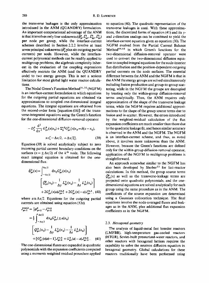
the transverse leakages is the only approximation introduced in the ANM (QUANDRY) formulation. An important computational advantage of the ANM is that it involves only four unknowns (~ , L-~gx, ~y, ~z) per node per group, while the interface-current schemes described in Section 2.2.2 involve at least seven principal unknowns (q~ plus six outgoing partial currents) per node. However, while the interface- current polynomial methods can be readily applied to multigroup problems, the algebraic complexity inherent in the evaluation of the coupling expressions effectively restricts the ANM (and the QUANDRY code) to two energy groups. This is not a serious limitation for most global light water reactor calculations.

The Nodal Green's Function Method 31.32 (NGFM) is an interface-current formulation in which equations for the outgoing partial equations are obtained via approximations to coupled one-dimensional integral equations. The integral equations are obtained from the second-order form [equation (16)] of the transverse-integrated equations using the Green's function for the one-dimensional diffusion-removal operator

d 2 - o~ ~ G~x(XlXo) + Z;'kG~(XlXo = 6(x- Xo),

xe[ -Ax /2 , + Ax/2]. (39)

Equation (39) is solved analytically subject to zero incoming partial current boundary conditions on the surfaces (x = + Ax/2) of the k th node. The following exact integral equation is obtained for the one- dimensional flux:

l ' a x l2

~x(x) = | dxoG;,,(XlXo) d - a x / 2

1 1 k [Qk,~(x0)- ~y L ~, (Xo) -- ~zz L,z (Xo) ]

k i n , k + 2Ggx(xla)J~x + + 2G~x(xl-aLl i"'k (40) / v f f X - ,

where a=Ax/2. Equations for the outgoing partial currents are obtained using equation (12c). j g o u t ,k l_,hk _ l i n , k

x ± ~ 2 W g x ± ~ g x ±

=½ I Ax/2 dxoG~x(+alxo ) d - a x / 2

I k 1 k 1 q P.gx(Xo)- ~ Lg,(~o) - ~ L;~(Xo)|

+ [G~x(ala)- ,1,i*.k + G~tal in,k --a)Jd:,T_ (41) - d ~ g x ±

The one-dimensional fluxes are expanded in quadratic polynomials with the expansion coefficients computed using a moments weighted residual procedure applied

to equation (40). The quadratic representation of the transverse leakages is used. With these approximations, the discretized forms of equation (41) and its y- and z-direction analogs can be combined to yield the interface-current equation given as equation (30). The NGFM evolved from the Partial Current Balance Method 44"45 in which Green's functions for the two-dimensional diffusion-removal operator were used to convert the two-dimensional diffusion equation to coupled integral equations for the node-interior flux distribution and the position-dependent outgoing partial currents on the node surfaces. The essential difference between the ANM and the NGFM is that in the ANM the energy groups are solved simultaneously including fission production and group-to-group scattering, while in the NGFM the groups are decoupled by treating only the within-group diffusion-removal terms analytically. Thus, the ANM requires only approximation of the shape of the transverse leakage terms, while the NGFM requires additional approximations to the shape of the group source terms due to fission and in-scatter. However, the errors introduced by the weighted-residual calculation of the flux expansion coefficients are much smaller than those due to the quadratic leakage fit, and hence similar accuracy is obseri, ed in the ANM and the NGFM. The NGFM is an interface-current scheme, and thus, as noted above, it involves more unknowns than the ANM. However, because the Green's functions are defined only for the within-group diffusion-removal operator, application of the NGFM to multigroup problems is straightforward.

An approach somewhat similar to the NGFM has also been developed by Shober 33 for fast-reactor calculations. In this method, the group source terms O kgx(x ) as well as the transverse-leakage terms are projected onto quadratic polynomials, and the one- dimensional equations are solved analytically for each group using the same procedure as in the ANM. The coefficients of the source expansion are determined using a Gaussian collocation technique. The final equations involve the node-averaged fluxes and leakages as in the ANM, plus additional flux expansion coefficients as in the NGFM.

2.3. Hexagonal geometry The analysis of liquid-metal fast breeder reactors

(LMFBR), high-temperature gas-cooled reactors (HTGR), Soviet-built pressurized-water reactors, and other reactors with hexagonal lattices requires the capability to solve the neutron diffusion equation in hexagonal geometry. Global calculations for these reactors traditionally have been performed using


conventional finite-difference methods applied on a uniform triangular grid introduced within each hexagonal fuel assembly. The success of the Cartesian- geometry nodal methods has prompted the development of analogous formulations 46-s° which can be applied directly on the hexagonal mesh. Other higher- order finite-difference schemes 51-54 have also been formulated in hexagonal geometry. As in Cartesian geometry both polynomial 47~9 and analytic 42'46'5° nodal approaches have been developed although, to date, only the polynomial methods have been applied to the one-dimensional equations obtained in the extension of the transverse-integration procedure to hexagonal geometry. In order to illustrate some important differences relative to the Cartesian-geometry case, we develop here a transverse-integrated polynomial method 45'49 which retains many of the features of the Cartesian-geometry formulation derived in Section 2.2.2.

For the sake of simplicity, we consider only two- dimensional hexagonal geometry in the following development. The extension to three-dimensional hexagonal-z geometry is straightforward, and the z- direction fluxes are approximated as shown in equation (18). The hexagonal node is defined in terms of local (x, y) coordinates:

Vk: (x, y) x ~ [ - h / 2 , +h/2], ye[-y~(x), +y~(x)],

1 y~(x) = ~ ( h - I x l ) , (42)

where h is the lattice pitch, and the x-axis is taken as perpendicular to one pair of opposite faces of the hexagon. The one-dimensional flux analogous to equation (14) is

1 I r,~:,) @kox(X) ~ 2~s(X) d-ys(x) dy dpko(x, y). (43)

However, because the y-direction mesh spacing depends upon x, it is more convenient to work with

- dy ¢kka(x, y). (44) d - y,(x)

In order to distinguish these fluxes, we refer to the flux in equation (44) as the partially-integrated flux, and denote it without the bar. The partially-integrated x- component of the net current is

O J~(x) -- [ r~tx) d y - D~ fix ~b,(x, y). (45)

d - ys(x)

Analogous partially-integrated fluxes and currents are defined for the two opposite faces. That is, the u- direction is rotated 60 ° counter-clockwise with respect

to the x-axis, and the v-direction is rotated 120 ° from the x-axis.

The P - 1 form of the transverse-integrated equations is derived by performing a simple neutron balance over the vertical strip defined by

6vk: (X, y) Xe.[X, x+dx] , ye[-y~(x), +y,(x)].

The result is

d . , ' k k dx J~x(x) + ~.o'~c~(x) = Q~(x)

2 x/3[J~(x, y~(x))-J~(x, -y~(x))], (46a)

where J~(x, + ydx)) are surface-normal components of the net current across the u- and v-directed faces. Applying Leibniz' rule for differentiating an integral with variable limits to equation (44) and then re- arranging yields

d J~x (x) - - D k dx dp~,,(x) + D~y'~(x)

[~b~(x, y~(x)) + dpkg(x, -- y.(x))], (46b)

where 1

y's(x) = - ~-j sgn(x). (47)

Note that equations (46) are the hexagonal-geometry analogs of equations (13).

It is clear that the partially-integrated net current introduced in equation (45) must be continuous over x e [ -h /2 , + h/2]. Therefore, with reference to equations (46b) and (47), it is also clear that the partially- integrated fluxes in the three hex-plane directions will exhibit first-derivative discontinuities of the form

lim - ~bkgx(x)

2o~ = ~/~ [~bk,(x, y~(x)) + c~k.(x, - ys(x))]x = o. (48)

This behavior, which does not appear in Cartesian geometry, must be represented by any polynomial used to approximate ~b~x(x ).

The partially-integrated fluxes in the three hex- plane directions are approximated by

d~:x(X)~2ys(x)[~Jk,+ ~=l a~,,.f.(x)], (49)

where k and k agxl agx2 are defined as in equations (21), and

X f~(x) - h = ~ (50a)

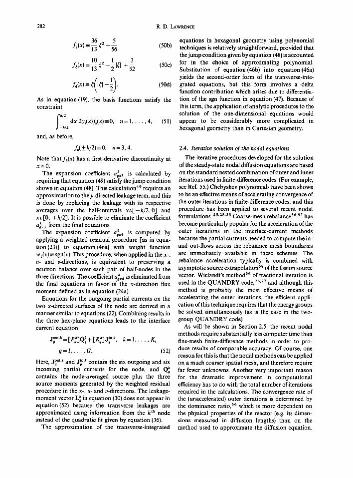
282 R.D. LAWRENCE

36 2 5 (50b) f2(x) - B ~ 56

10 2 1 3 f3(x) = ~ ~ -- ~ Ill + ~ (5Oc)

f4(x) =- ~(1~1- ~). (50d)

As in equation (19), the basis functions satisfy the constraint

f h/2 dx 2ys(x)f,(x)=O, n = 1 . . . . . 4, (51) -hi2

and, as before,

f,(+_h/2)=-O, n=3, 4.

Note that f3(x) has a first-derivative discontinuity at x=0 .

The expansion coefficient aox 3k is calculated by requiring that equation (49) satisfy the jump condition shown in equation (48). This calculation 49 requires an approximation to the y-directed leakage term, and this is done by replacing the leakage with its respective averages over the half-intervals x e [ - h / 2 , 0 ] and xe[O, + hi2]. It is possible to eliminate the coefficient

k from the final equations. agx3 The expansion coefficient agx4k is computed by

applying a weighted residual procedure [as in equation (23)] to equation(46a) with weight function wl(x ) = sgn(x). This procedure, when applied in the x-, u- and v-directions, is equivalent to preserving a neutron balance over each pair of half-nodes in the three directions. The coefficient k is eliminated from aox4 the final equations in favor-of the x-direction flux moment defined as in equation (24a).

Equations for the outgoing partial currents on the two x-directed surfaces of the node are derived in a manner similar to equations (22). Combining results in the three hex-plane equations leads to the interface current equation

out,k - - k k [ - R k ' ] J i n , k Jg - [Pg]Qg + k = 1, K, t . - - f f . i - - f f , • • •

g = 1 . . . . . G. (52)

Here, jo,t.k and .I in'k contain the six outgoing and six - - f f - - f f

incoming partial currents for the node, and Q~ contains the node-averaged source plus the three source moments generated by the weighted residual procedure in the x-, u- and v-directions. The leakage- moment vector L~ in equation (30) does not appear in equation (52) because the transverse leakages are approximated using information from the k th node instead of the quadratic fit given by equation (36).

The approximation of the transverse-integrated

equations in hexagonal geometry using polynomial techniques is relatively straightforward, provided that the jump condition given by equation (48) is accounted for in the choice of approximating polynomial. Substitution of equation (46b) into equation (46a) yields the second-order form of the transverse-integrated equations, but this form involves a .delta function contribution which arises due to differentia- tion of the sgn function in equation (47). Because of this term, the application of analytic procedures to the solution of the one-dimensional equations would appear to be considerably more complicated in hexagonal geometry than in Cartesian geometry.

2.4. Iterative solution of the nodal equations

The iterative procedures developed for the solution of the steady-state nodal diffusion equations are based on the standard nested combination of outer and inner iterations used in finite-difference codes. (For example, see Ref. 55.) Chebyshev polynomials have been shown to be an effective means of accelerating convergence of the outer iterations in finite-difference codes, and this procedure has been applied to several recent nodal formulations. 25,28,33 Coarse-mesh rebalance 56"57 has become particularly popular for the acceleration of the outer iterations in the interface-current methods because the partial currents needed to compute the in- and out-flows across the rebalance mesh boundaries are immediately available in these schemes. The rebalance acceleration typically is combined with asymptotic source extrapolation 5s of the fission source vector. Wielandt's method 56 of fractional iteration is used in the QUANDRY code, 26'27 and although this method is probably the most effective means of accelerating the outer iterations, the efficient application of this technique requires that the energy groups be solved simultaneously (as is the case in the two- group QUANDRY code).

As will be shown in Section 2.5, the recent nodal methods require substantially less computer time than fine-mesh finite-difference methods in order to produce results of comparable accuracy. Of course, one reason for this is that the nodal methods can be applied on a much coarser spatial mesh, and therefore require far fewer unknowns. Another very important reason for the dramatic improvement in computational efficiency has to do with the total number of iterations required in the calculations. The convergence rate of the (unaccelerated) outer iterations is determined by the dominance ratio, 56 which is more dependent on the physical properties of the reactor (e.g. its dimensions measured in diffusion lengths) than on the method used to approximate the diffusion equation.

Nodal diffusion and

On the other hand, the convergence rate of the inner iterations is determined by the spectral radius 56 of the associated iteration matrix, and this number is very sensitive to the choice of mesh spacings. For a given spatial approximation, the spectral radius increases (and thus the convergence rate decreases) as the spatial mesh becomes finer. Therefore, for these reasons, the nodal and finite difference methods require roughly the same number of outer iterations (although this depends upon the choice of acceleration techniques as well as the degree of convergence achieved during the inner iterations), but the nodal schemes, because they are applied on a much coarser spatial mesh, require far fewer inner iterations per outer iteration. Thus, simply stated, the nodal methods involve fewer unknowns, and these unknowns are recomputed far fewer times than in conventional finite-difference methods applied on a fine mesh.

The inner iterations in the interface-current methods consist of sweeps through the mesh for the purpose of computing all partial currents for a given group. Since equation (30) is derived by combining results from each coordinate direction, an obvious iterative procedure 2s.31 in Cartesian geometry is to solve first for the x-directed partial currents on each x-line of the mesh, followed by all y-directed and then all z-directed partial currents. For each direction, the transverse leakage terms are computed using the most recently available partial currents in the two transverse directions. A more computationally efficient algorithm, which accesses the partial current data in a more linear fashion, is obtained by sweeping the axial mesh planes in a one-dimensional (odd-even) checkerboard order- ing, i.e. the odd-numbered planes are processed first followed by the even-numbered planes. The x- and y- directed partial currents for each plane are computed from equation (30) using a red-black checkerboard sweep on the plane. The outgoing z-directed partial currents are then computed using a sequential sweep of the nodes on the plane. This procedure is easily extended to hexagonal geometry, where the hex-plane partial currents are computed using a 'four-color' checkerboard sweep. 46'47 If unity discontinuity factors are used in equation (6), the incoming partial currents are simply outgoing currents from neighboring nodes; otherwise, the following interface condition is used:

. x + = [ J ; ~ - + ~ J ; x + ], L I - J

where

and the x + surface of the k ,h node corresponds to the

transport methods 283

x- - surface of the neighboring I th node. For light- water reactor problems on an assembly-size mesh, only one or two checkerboard partial current sweeps typically are required for each group at each outer iteration. Optimized finite-difference codes, 55 on the other hand, require at least 10 inner iterations when applied on the fine spatial mesh necessary for acceptable accuracy.

A very efficient iterative strategy based on the use of discontinuity factors has been developed indepen- dently by Koebke 1°'59'6° and Smith. 61 To demonstrate, suppose we have available both a higher-order method (e.g. a nodal diffusion or a nodal transport scheme) and a corresponding lower-order method (e.g. a mesh-centered finite-difference diffusion method or a nodal diffusion method, respectively). Using discontinuity factors, it is possible to modify the coupling relationships in the lower-order scheme such that they will reproduce exactly the known interface net currents computed with the higher-order method. Therefore, instead of solving the higher-order equations at each step of the calculation, the majority of the computational effort may be shifted to the less expensive solution of the lower-order equations, with coupling coefficients (i.e. discontinuity factors) periodically updated in order to match the most recent iterate of the higher- order method. Smith's approach was developed for the primary purpose of reducing the amount of storage required for the coupling coefficients in QUANDRY. Koebke 59 has applied this approach to the solution of nodal transport equations (discussed in Section 3.3), as well as to the solution of the NEM equations using a low-order flux approximation [N = 2 in equation (18)] as the lower-order scheme. 1°'6° The procedure out- lined here can be applied to all of the nodal diffusion methods discussed in this paper.

2.5. Numerical examples

2.5.1. The Cartesian-geometry IAEA benchmark problem. The IAEA benchmark problem 62 has been an important standard used to measure progress in the development of coarse-mesh diffusion-theory methods. Although this problem represents a highly simplified model of a pressurized water reactor, the large thermal flux gradients at the core-reflector interface present a severe (and reasonable) test of numerical diffusion-theory methods. The problem is specified using two energy groups, and both two- and three-dimensional models have been defined. The two- zone core consists of 177 (homogenized) fuel assemblies 20 cm on a side, and is reflected radially and axially by 20 cm of water. Each of nine fully inserted control rods is represented as a smeared absorber within a single homogenized fuel assembly. Four additional

284 R.D. LAWRENCE

partially inserted control rods are included in the three-dimensional model.

Comprehensive numerical comparisons for the two- dimensional configuration have been given in Refs 7 and 32, and Table 1 summarizes nodal and finite- difference results for the three-dimensional IAEA problem. The errors are with respect to a reference solution 62,63 obtained by extrapolation of the finite difference results. A reasonable accuracy criterion is that the assembly-averaged power densities be computed to within 2% of the reference solution, and each of the nodal methods shown in Table 1 achieves this level of accuracy using a uniform 20 cm mesh. The mesh-centered finite-difference method requires a very fine mesh, 1.67 cm in the radial direction and 3.33 cm axially, in order to obtain similar accuracy. The original finite-difference calculations 63 used an older version of the VENTURE code 64, and two of these calculations were repeated using the optimized finite- difference option 5S'65 in the DIF3D code in order to obtain more realistic computing times for these calculations. Using these DIF3D calculations as a basis, it appears that the 1.67 cm finite-difference calculation might require roughly 2hr on the IBM 370/195, or at least two orders of magnitude more c6mputing time than the nodal calculations.

In comparing the nodal results shown in Table 1, it is necessary to note that the extrapolated finite- difference solution used as a reference is probably not fully converged spatially, and therefore the errors with respect to the true diffusion-theory reference solution may differ slightly from those shown in Table 1. The

nodal methods all use the quadratic leakage fit shown in equation (35), but we expect the QUANDRY solution to be the most accurate because, unlike the other methods, this is the only approximation introduced in this method. The small errors observed in the QUANDRY calculation thus demonstrate the very acceptable accuracy of the quadratic leakage approximation. The polynomial methods use either N = 4 (DIF3D) or N = 5 (NEM and NODLEG) in equation (18), and the fact that the errors are only slightly larger than the QUANDRY errors indicate that the one-dimensional fluxes are adequately approximated by these polynomials. A fortuitous cancellation of the errors due to the leakage representation and the weighted-residual flux approximation in the N G F M is apparently responsible for the smaller value of em~ x in the N G F M calculation. Comparison of the execution times is complicated by the use of different computers and planar symmetry options. However, after adjust- ing for these factors, the QUANDRY execution time appears to be the smallest, as would be expected based on the smaller number of unknowns. The remaining methods are all based on interface-current formulations, and the NEM and the DIF3D nodal method appear to be somewhat faster than the N G F M and the NODLEG method, probably due to more efficient iteration strategies. Independent of the question of which method is faster, one conclusion is clear: recent nodal methods, using either polynomial or analytic approximations to the transverse-integrated equations, are capable of very high accuracy in LWR calculations with one node per assembly, and for

Table 1. Comparison of nodal and finite difference results for the three-dimensional IAEA benchmark problem a

Radial/axial mesh CPU

Method Reference spacings (cm) kef f ek(% ) era,z(% ) Time b (min) Computer

Polynomial nodal DIF3D/NODAL 30 20.0/20.0 1.02898 -0.005 1.5 0.3/0.4 IBM 370/195 NEM 22,63 20.0/20.0 1.02911 +0.008 0.9 1.0/-- CDC 6600 NODLEG 29 ,66 20.0/20.0 1.02895 -0.008 1.3 1.7/-- CDC 6600

Analytic nodal ANM (QUANDRY) 26 ,27 20.0/20.0 1.02902 -0.001 0.7 0.2/0.3 IBM 370/195 NGFM 32 20.0/20.0 1.02909 +0.006 0.4 --/1.0 CYBER 175

Finite difference VENTURE 63,64 5.0/10.0 1.02864 -0.039 13.7 --/49 IBM 360/91 VENTURE 63,64 2.5/5.0 1.02887 -0.016 4.9 --/192 IBM 360/91 VENTURE 63,64 1.67/3.33 1.02896 -0.007 2.1 --/360 IBM 360/195 DIF3D 55,65 5.0/10.0 1.02864 -0.039 13.7 --/3 IBM 370/195 DIF3D 55,65 2.5/5.0 1.02887 -0.016 4.9 --/40 IBM 370/195

"e k =error in kef f with respect to reference eigenvalue (1.02903). era, z = maximum error in assembly-averaged power densities.

b The execution times are for calculations using eighth-core/quarter-core planar symmetry.

Nodal diffusion and

comparable accuracy, very substantial reductions in computer time are observed relative to optimized finite-difference codes. However, it is important to note that the IAEA problem involves spatially- constant cross sections within each node, and the inclusion of space-dependent burnup and nonlinear feedback can introduce additional errors beyond the spatial truncation errors considered here. The accurate modeling of such effects requires either the use of a finer spatial mesh (e.g. 2 by 2 within each fuel assembly), or an explicit representation of the spatial dependence ofthe cross sections within the node. 23

2.5.2. The hexagonal-geometry SNR benchmark problem. The SNR benchmark problem 67"6s is a 4-group model of a 300 MWe homogeneous-core LMFBR originally specified in both Cartesian and triangular geometries. The modified problem 6s solved here is obtained by altering the outer boundary of the triangular-geometry model (while preserving the volume of the core) to allow imposition of boundary conditions along surfaces of hexagons. The model consists of a two-zone core surrounded by radial and axial blankets without a reflector. The height of the active core is 95 cm, and each axial blanket is 40 cm thick. A total of 11 rings of hexagons (including the central hexagon) are included in the model, with a lattice pitch of 11.2003 cm. Vacuum boundary conditions are imposed on the outer surfaces of the blankets. The full-core model includes a total of 18 control rods, with 6 of these rods parked at the core-upper axial blanket interface, and the remaining 12 rods inserted to the core midplane. All calculations were performed using sixth-core planar symmetry.

Results for the three-dimensional SNR benchmark


problem are summarized in Table 2. The calculations were done using the hexagonal-geometry nodal option 49"69 and the mesh-centered triangular-geometry finite-difference option 65 in the DIF3D code. The finite-difference calculations used either 6 or 24 triangular mesh cells per hexagonal fuel assembly, and the nodal calculations used the hex-plane approximation shown in equation (49) in combination with a cubic axial approximation [ N = 3 in equation (18)'1. The calculations with 8 and 18 axial mesh planes used 4 and 10 mesh planes, respectively, in the active core, and 2 and 4 mesh planes, respectively, in each axial blanket. Extrapolated results assuming an infinite number of axial mesh planes have been included in order to allow isolation of the errors due to the axial approximations in the nodal and finite difference schemes. For example, these results show that the 0.16% eigenvalue error in the 8-plane nodal calculation involves contributions of 0.13 % and 0.03 % due to the hex-plane and axial approximations, respectively. Similar analysis of the finite difference results shows that the axial contribution to the total eigenvalue error in the 18-plane and 36-plane calculations is 0. 30% and 0.074).08%, respectively. Similar trends are observed in the flux errors, although there is some fortuitous cancellation of hex-plane and axial errors in the finite- difference results for the inner core and radial blanket. We conclude that the axial accuracy of the nodal scheme with 8 axial planes is superior to that of the finite difference approximation using 36 planes. Furth- ermore, although the overall accuracy of the 8-plane nodal calculation is superior to that of the 36-plane 6 triangles-per-hexagon finite difference results, the nodal calculation required a factor of 8 less computing time than this finite difference calculation.

Table 2. Comparison of nodal and finite-difference results for the three-dimensional SNR benchmark problem a

No. of CPU Method axial planes kef f £K(%) eic(O//o) eoc(%) eR,(%) CA.(%) ~CR(%) Time (min)

DIF3D (NODAL) 8 1.01150 0.16 -0.17 0.23 0.95 -0.30 -0.60 0.2 DIF3D (NODAL) 18 1.01125 0.13 -0.18 0.22 0.96 -0.11 -0.44 0.6 DIF3D (NODAL) ~ 1.01120 0.13 -0.18 0.22 0.96 -0.07 -0.39 --- DIF3D (6A) 18 1.01505 0.52 -0.18 0.52 0.22 -2.55 -2.56 0.6 DIF3D (6A) 36 1.01280 0.29 -0.27 0.42 0.47 -0.60 - 1.72 1.6 DIF3D (6A) oo 1.01205 0.22 -0.29 0.38 0.56 -0.06 - 1.44 --- DIF3D (24A) 18 1.01342 0.35 -0.05 0.23 -0.20 -2.61 - 1.48 3.1 DIF3D (24A) 36 1.01118 0.13 -0.04 0.13 0.05 -0.64 -0.64 6.0 DIF3D (24A) oo 1.01043 0.05 -0.08 0.09 0.14 0.02 -0.36 -- Reference b - - 1 .00989 . . . . . . . .

"e~c, eoc , era , eAa, and ecR, are errors in the group- and region-averaged fluxes for the inner core, outer core, radial blanket, axial blanket, and control rod regions, respectively.

b The reference solution is obtained by Richardson extrapolation of the DIF3D(6A)-18 plane and DIF3D(24A)-36 plane solutions.

286 R.D. LAWRENCE

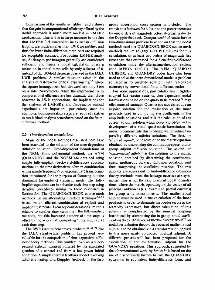
Comparison of the results in Tables 1 and 2 shows that the gain in computational efficiency offered by the nodal approach is much more modest in LMFBR applications. This is due in large measure to the fact that LMFBR fuel assemblies, measured in diffusion lengths, are much smaller than LWR assemblies, and thus far fewer finite-difference mesh cells are required for acceptable accuracy. For routine LMFBR analy- ses, 6 triangles per hexagon generally are considered sufficient, and hence a nodal calculation offers a reduction in radial mesh cells by only a factor of 6, instead of the 100-fold decrease observed in the IAEA LWR problem. A similar situation exists in the analysis of fast-reactor critical experiments, 3° where the square homogenized fuel 'drawers' are only 5 cm on a side. Nevertheless, while the improvements in computational efficiency are less dramatic than those observed in LWR applications, the implications for the analysis of LMFBR's and fast-reactor critical experiments are important, particularly since no additional homogenization steps are required relative to established analysis procedures based on the finite- difference method.

2.6. Time-dependent formulations Many of the nodal methods discussed here have

been extended to the solution of the time-dependent diffusion equation. Time-dependent formulations of the NEM, Sim's polynomial method, the ANM (QUANDRY), and the NGFM are obtained using simple fully-implicit (backward-difference) approximations to the time derivatives, often in combination with a simple 'frequency' (or 'exponential') transformation introduced for the purpose of factoring out the dominant (asymptotic) transient mode. The fully- implicit equations can be solved at each time step using iterative procedures similar to those discussed in Section 2.4. The QUABOX/CUBBOX coarse-mesh methods use an alternating direction technique 34'35 based on an efficient combination of explicit and implicit treatments. Accuracy considerations limit this scheme to smaller time steps than the fully-implicit methods, but this increased number of time steps is offset by the very small computing times required at each time step.

The BWR kinetics benchmark problem, 62'68'7° like the IAEA steady-state problem, has proved very valuable for the comparison of time-dependent diffusion-theory methods. This problem involves a super- prompt critical transient initiated by the simulated ejection of a control rod from a low-power initial condition. A simple thermal feedback model involving adiabatic heatup and Doppler feedback in the fast-

group absorption cross section is included. The transient is followed for 3.0 s, and the power increases by nine orders of magnitude before decreasing due to the Doppler feedback. Comparison 32 of results for the two-dimensional problem have shown that the nodal methods (and the QUABOX/CUBBOX coarse-mesh method) require roughly 1-3 CPU minutes for this calculation, or at least two orders of magnitude less time than that estimated for a 5 cm finite-difference calculation using the alternating-direction explicit code MEKIN (Ref. 71). The NEM, QUABOX/ CUBBOX, and QUANDRY codes have also been used to solve the three-dimensional model, a problem so large as to preclude solution (with reasonable accuracy) by conventional finite-difference codes.

For some applications, particularly small, tightly- coupled fast-reactor systems, time-dependent nodal formulations based on the quasi-static method 72 may offer some advantages. Quasi-static models require an adjoint solution for the evaluation of the inner products used in computing the coeffÉcients of the amplitude equations, and it is the calculation of the correct adjoint solution which poses a problem in the development of a nodal quasi-static formulation. In order to demonstrate this problem, we introduce two possibly different adjoint solutions. The first, or 'physical adjoint', is the solution to the matrix equation obtained by discretizing the continuous-space, multigroup adjoint diffusion equation. The second, or 'mathematical adjoint', is the solution to the matrix equation obtained by discretizing the continuous- space, multigroup forward diffusion equation, and then transposing the coefficient matrices. The two adjoints are equivalent in finite-difference diffusion- theory methods since the leakage r0atrices are symmetric. This is not the case in recent nodal formulations, where the matrix operating on the vector of all principal unknowns (e.g. fluxes and partial currents) for group g is nonsymmetric. The mathematical adjoint must be used in the calculation of the inner products in order to eliminate first-order errors in the reactivity expression, but direct calculation of this solution is complicated by the unusual coupling introduced by transposing the in-group nodal coefficient matrices. However, as shown in recent work 73 on nodal perturbation theory, the required mathematical adjoint can be obtained via a transformation applied to the more easily computed physical adjoint. A different procedure 74 has been proposed for the calculation of the mathematical adjoint for the QUANDRY equations. This approach, suggested by the aforementioned work by Smith, 61 is based on the use of discontinuity factors to cast the QUANDRY equations in equivalent finite-difference form, and


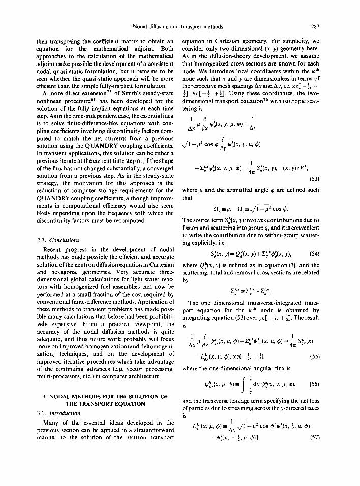
then transposing the coefficient matrix to obtain an equation for the mathematical adjoint. Both approaches to the calculation of the mathematical adjoint make possible the development of a consistent nodal quasi-static formulation, but it remains to be seen whether the quasi-static approach will be more efficient than the simple fully-implicit formulation.

A more direct extension 7s of Smith's steady-state nonlinear procedure 6~ has been developed for the solution of the fully-implicit equations at each time step. As in the time-independent case, the essential idea is to solve finite-difference-like equations with coupling coefficients involving discontinuity factors computed to match the net currents from a previous solution using the QUANDRY coupling coefficients. In transient applications, this solution can be either a previous iterate at the current time step or, if the shape of the flux has not changed substantially, a converged solution from a previous step. As in the steady-state strategy, the motivation for this approach is the reduction of computer storage requirements for the QUANDRY coupling coefficients, although improvements in computational efficiency would also seem likely depending upon the frequency with which the discontinuity factors must be recomputed.

2.7. Conclusions Recent progress in the development of nodal

methods has made possible the efficient and accurate solution of the neutron diffusion equation in Cartesian and hexagonal geometries. Very accurate three- dimensional global calculations for light water reactors with homogenized fuel assemblies can now be performed at a small fraction of the cost required by conventional finite-difference methods. Application of these methods to transient problems has made possible many calculations that before had been prohibiti- vely expensive. From a practical viewpoint, the accuracy of the nodal diffusion methods is quite adequate, and thus future work probably will focus more on improved homogenization (and dehomogenization) techniques, and on the development of improved iterative procedures which take advantage of the continuing advances (e.g. vector processing, multi-processors, etc.) in computer architecture.

3. NODAL METHODS FOR THE SOLUTION OF THE TRANSPORT EQUATION

3.1. Introduction Many of the essential ideas developed in the

previous section can be applied in a straightforward manner to the solution of the neutron transport

equation in Cartesian geometry. For simplicity, we consider only two-dimensional (x-y) geometry here. As in the diffusion-theory development, we assume that homogenized cross sections are known for each node. We introduce local coordinates within the k th node such that x and y are dimensionless in terms of the respective mesh spacings Ax and Ay, i.e. xe[-½, +

y [ - ~ , +½]. Using these coordinates, the two- dimensional transport equation 76 with isotropic scattering is

1 O k 1 Axx " ?xx O°(x' y' "' 49) + Ay

k cos th ~yy O.(x. y, , . 4~)

1 k + x~k¢¢~, y. f,. 6 ) = ~ s , (~ . y). (x. y ) e V k,

(53)

where # and the azimuthal angle ~b are defined such that

f~x-#, fJr---x/1 _ . 2 COS q~.

The source term S~(x, y) involves contributions due to fission and scattering into group 9, and it is convenient to write the contribution due to within-group scattering explicitly, i.e.

S~o(x. y)= Q~(x. y)+ Z;'k~b~(x. y). (54)

where Q~(x. y) is defined as in equation (3). and the scattering, total and removal cross sections are related by

y~.k_ zt.k E~.k O - - - -g - - - -9 "

The one dimensional transverse-integrated transport equation for the k 'h node is obtained by integrating equation (53) over ye [ - ½, + ½]. The result is

1 ~ k ~,k k 1 - - 4))+~ O.~(x,., S~x(X)

k -L,,(x. ,. 4,). xe(-½. +½). (55)

where the one-dimensional angular flux is 1

k X f - - ~kox ( . , . ~b) i dy ~Oko(x. y. , . qS). (56)

and the transverse leakage term specifying the net loss of particles due to streaming across the y-directed faces is

1 2 L k,(x, = c o s , .

- ~bko(x. -- ½... q~)]. (57)

288 R.D. LAWRENCE

The nodal approximations developed in the following subsections are derived from the integral form of equation (55) obtained by solving equation (55) as a simple ordinary differential equation in the x variable. For/~ > 0, the integral form is

dx o - exp[ - Y.(x - xo)/la] O~x(X, l, >o, 4))= Ax _~ #

S ~ x ( X o ) - L a r ( X o , / z>O, 4~)

in ,k + O~x- (~, 4~)exp[ - l~(x + ½)/~],

(58)

where

~ i n , k ( k 1 ~- ,~ , 4,)= ¢) ~'a~(- ~, ~>0,

is the incoming angular flux on the left (or minus-x directed) surface of the node, and

Z -- l~'*Ax.

Evaluating this result at x = + ½ yields an equation for the outgoing angular flux across the right (plus-x directed) surface of the node:

f - I 1 o~t,k x e x p [ - 1~(½- Xo)//~ ] ~a-~ + (1~, dp) = A ~ d x o

in ,k + 0g~-(~t, q~)exp[ - E//O. (59)

Solving equation (55) for /~<0 yields two similar equations for 0~(x,/l < 0, ¢) and qJax"k'- t#, ¢). Repeating this procedure in the y-direction yields four analogous equations.

Two classes of angular approximations will be discussed here. The first, developed in Section 3.2, is based on a conventional multidimensional discrete- ordinates approximation of the angular dependence. In Section 3.3, an alternate approach is developed in which the angular dependence of the surface fluxes is represented by a low-order double P, expansion. A comparison of numerical results obtained using the different angular representations is given in Sec- tion 3.4.

3.2. N o d a l d iscre te ord inates me thods

The methods in this class can be viewed as higher- order spatial approximations to the multidimensional discrete-ordinates equations. An attractive feature of these schemes is that they converge to the exact solution of the discrete-ordinates equations in the limit of infinitely-fine spatial mesh. Included in this class of

methods are the Discrete Nodal Transport Method 77-79 (DNTM), the TWOTRAN nodal method 8°-s2 due to Waiters, and an exponential expansion method 83'84 developed by Pevey. In order to illustrate these methods, we begin with the basic development of the DNTM, and then indicate some extensions and modification to this basic formulation.

In the following development, we denote the i tla

ordinate by the direction cosines (/a i, q.), where r / -

f~r=x/1 - # ~ cos ~b. Equations (58) and (59) are evaluated along the i th ordinate, and thus

Okox(x, ~>0, ~)- ,¢#x , u,, ~,), ~,>0,

and so on. The one-dimensional spatial dependence of the node-interior fluxes and sources, and the spatial dependence of the transverse leakage terms are expanded in low-order polynomials:

N /c ~ k Oar( x , Izi, qi) = ~, a.Oax.(~ i, r l ) f . (x ) , 0<N<2,_ _ (60a)

n = 0

N

S~ox(x) ~- ~, a.S~x.f.(x) (608) n = 0

N S k , ~ Lay (x, I&, rli) = ~. * a .Lay. (Ui, rl~)f.(x), N S < N , (60e)

n = 0

where, as in equations (20),

fo(x) =- 1

L ( x ) = x

f~(x)- 3x 2_ -I.

The constants a. are defined by 1

f 1 _ ~ dx[f.(x)] 2, [a.] -½

and thus

ao= 1

a1=12

a 2 = 20.

Although the original DNTM formulation 79 used Legendre polynomials as the basis functions, the slightly modified form shown in equation (60) is used here so that the resulting spatial moments for the scalar flux are identical to those employed in the diffusion-theory development in Section 2.2.2. As in equation (24a) [with w , ( x ) = f , ( x ) ] , the scalar-flux moments are given by

1

dpax. - dxdp~,(x) f . (x) . (61) -½

and thus k q~,,o is the node-averaged flux. The scalar-


flux moments are computed as in any discrete- ordinates method, i.e,

1

rkka~. = ~ w,~bk~,(#i, r/i), (62) i = 1

where w i are the angular quadrature weights. Equa- tions (60a) and (62) imply the following expansion of the scalar flux:

N

#akox(X) ~-- ~ a.~kox.f.(x). (63) n = O

The source moments sk~. in equation (60b) can be computed from the scalar-flux moments.

An equation for the spatial moments of the angular flux is obtained using a moments weighted residual procedure very similar to that described in Sec- tion2.2.2. Substituting equations(60) into (58), weighting with f,,(x), m = 0 . . . . . N, and then integrating over x~(-½, +½) yields

*~(/~i, r/,)= [Gg~(U,)] {S~-Lko,(#i, qi)} x + in,k +[Gg (#i)]~bg~_(#i, th), /~i>0. (64)

where ,kg~, Skgx, and Lkgy are vectors containing the respective spatial moments. Substituting equations (60b) and (60c) into equation (59) yields the discretized equation for the outgoing angular flux on the right surface:

~/out,k~ + x T k k ,~, + t#i, r/i) = [Go (#,)] {Sg~- Lg,(/~ i, r/i)} + d xin,k ~g~_ e x p [ - E//~/h #i > 0. (65)

The entries of the matrices shown in equations (64) and (65) involve weighted integrals of the exponentials appearing in equations (58) and (59), and the unique entries of these matrices can either be pre-computed and stored or re-computed during the mesh sweeps.

Several different approximations for the transverse leakage terms have been developed. The original DNTM formulation used a flat approximation [as in equation (37)] in which the x-dependent leakage is replaced by its average value over the node. Thus, NS--O in equation (60c), and from equation (57) we find

k l t k Lg~,o (Hi, r/i) = ~yy r/ i [O;;:; (#,, r/i)

~ i n , k -q~gr-t/~i, ql)], r/i >0. (66)

Construction of higher-order approximations to the transverse leakage requires calculation of additional moments in the leakage expansion [equation (60c)]. From equation (57), it is clear that the higher-order leakage moments involve additional spatial moments of the angular fluxes on the two transverse surfaces.

Since only average (zero-moment) values of these fluxes are available from the solution of equation (65) and its y-direction analog, one possibility is to use adjacent-node information as in the quadratic leakage fit utilized nodal diffusion theory. For example, if #i>0, r/i>0, the linear m o m e n t Lgkyl(#i, r/i) can be computed by fitting the average fluxes on the y- directed faces of the k th node and the node immediately to its left. More elaborate fits which employ additional information are also possible, but one suspects that fitting procedures in general will be less accurate in transport theory than in diffusion theory because of the more rapid spatial variations exhibited by the angular current than by the scalar current. Neverthe- less, numerical tests s5 of this linear fitting procedure showed substantial improvements in accuracy relative to the fiat approximation, although iterative convergence difficulties ultimately forced this scheme to be abandoned, s6

A more rigorous approach s°'ss to the calculation of the leakage moments is based on the introduction of additional equations 7 for the spatial moments of the surface angular flux. To illustrate, we introduce the 'transverse' flux moment

1 ;f Oko:,T( x, I1i, r/i) -- dy yOko(x, y,/-t i, r/ih (67)

and note that this moment, evaluated at x = ½ (right surface), can be used to construct a linear approximation to the y-dependent flux on the right surface, e.g.

out,k 1 ~out,k~ qJgx + ~gi,

12--out,k • , + ~llgxT+l, lli, r/i)Y, /2i> 0. (68)

The analogous expansion on the top (y +) surface is out,k 1 ~ out,k 0g (x, ~, ~i, r/i)= ~0gr + (Ul, r/i)

l ~--out.k, + z~0rr+U~i, r/i)x, r/i>0. (69)

Note that this expansion has the same form as the linear expansion [ N S - 1] in equation (60c) and thus the following expression is obtained for the first moment of the transverse leakage:

Lgkl (#i' r/i)

= ~ y r l ~ / g y ~ + t ~ / i , r / i out k , r / i ) - - ~lgyTin'k- (/ti ' r/i)], r/i > 0. (70)

An equation for the transverse flux moment defined in equation (67) is obtained by operating on the discrete- ordinates form of equation (53) with

l

f~l dyy ,

290 R.D. LAWRENCE

to yield

/~ 0 k q~)+ ~o ~gxT(X, I~, q~) Ax a-x ~oxr(X, ~ , ,.~ k

=S~xT(X)-- rti ~,k, 1 2~y L~U°tx' ~'/~i, qi)

.~ ~]ko(x, - - 2'1 [~i' I~i ) -- 2~b~(x,/~i, q,)]- (71)

Equation (71) is converted to an integral form similar to equation (59), and the resulting equation approximated to yield the required equations for the linear moments of the surface fluxes. No additional node- interior unknowns are introduced if, as in Ref. 80, the two-dimensional source is represented using equation (60b) and its y-analog without cross terms:

Sk(x, y) ~ ~ + 12Sko,,, x + 12sok,, y, (72)

which leads to

k ~ k S~x T (X) = SOy 1"

Numerical comparisons a°'8~ have shown that the linear surface-flux approximation described here yields improved accuracy relative to the flat approximation; however, as will be discussed below, the computing time per mesh cell can be considerably greate~ for the linear surface approximation due to the increased number of surface unknowns.

Equations for the transverse surface-flux moments were first introduced in Ref. 7 for the purpose of reconstructing the intra-node flux shape from the results of a converged nodal solution. The essential idea of the reconstruction scheme 7 is to use the transverse-moments equations to compute the cross- term coefficients of a full biquadratie expansion of the node-interior flux. Walters 8° used these same equations in the manner described above to compute the linear surface moments required for his linear leakage approximation. The original DNTM formulation 79 used quadratic and constant approximations [i.e. N = 2 and NS=O in equations(60)] to the node- interior sources and leakages, respectively; following the terminology used in Ref. 80, we refer to this as the constant-quadratic (CQ) approximation. Waiters 8° combined his linear surface-flux approximation with a linear source representation, and this LL formulation subsequently has been extended to three dimensions, av

The nodal discrete-ordinates equations are solved using directed sweeps through the mesh very similar to those used in standard S u codes. 76 Consider the ease for /~ > 0, t/~ > 0. The in-flow information on the left and bottom surfaces is available from the calculations of the outflow in adjacent nodes processed during the current mesh sweep. The node-interior source infor-

mation is available from either the previous outer iteration (fission source) or the previous inner iteration (within-group scattering source). Using this information, the outflow quantities on the right and top surfaces can be computed using equation (65), and its y-analog, and, in the case of the linear surface-flux approximation, the two additional equations for first moments of the surface fluxes. These equations are coupled through the transverse-leakage terms, but they can be solved simultaneously for the average fluxes and flux moments on the outgoing surfaces:

i ~ o u t , k i . + t~,. 7 , ) - - [ e~ ( l , , . ~ , ) ] s . ~

+l-Tk(/t,, ~/,)]~-_.k(#,, q,), # ,>0, r/,>0. (73)

Here, q;~,k contains the out-flow information on the top and right surfaces, d~ i".k contains the in-flow

T 0 --

information on the left and bottom surfaces, and Sk0 contains the spatial moments of the node-interior source. Equation (73) represents a 2 by 2 system for the constant leakage approximation, and a 4 by 4 system for the linear surface-flux approximation. (In three dimensions, this becomes a 9 by 9 system involving an average flux and two transverse flux moments on each of the three outgoing faces.) At each node encountered in a sweep for a specified ordinate, equation (73) is solved to yield the out-flow data, and then this information is used in equation (64) to compute the node-interior flux moments.

As noted above, the increased complexity introduced by the linear surface-flux approximation leads to much longer execution times per mesh cell than in the constant leakage case. For this reason, Waiters sl,82 has developed a simplified linear-linear scheme [which he refers to as the linear nodal (LN) formulation] where the coupling inherent in equation (73) is reduced by neglecting the linear moment of the leakage term appearing in the equation for the first moment of the surface flux. This additional approximation makes it possible to cast the equations in an 'augmented' a2 weighted-difference form in which the weights do not depend upon the solution itself. These equations are solved by first computing the average angular flux in the node, and then extrapolating (analogous to the usual diamond-difference algorithm) to obtain the outflow information. The use of the augmented weighted-difference formulation makes possible a significant reduction in the computational effort relative to the solution of the (exact) linear-linear equations east in the form shown in equation (73). A very similar procedure has been reported in Ref. 88, where it is stated that the (exact) linear-linear equations can be cast in an augmented weighted-difference form. However, the coefficients in the final equations

Nodal diffusion and

shown in Ref. 88 are derived using the same simplifying approximation as introduced in Waiters' simplified linear-linear method.

The approximations used in the linear-linear nodal discrete-ordinates method are very similar to those used in the linear characteristic (LC) method, s9'9° Both methods assume a linear variation of the angular flux along the in-flow surface, and both assume the linear source representation shown in equation (72). Using these approximations, the LC method solves analytically for the two-dimensional angular flux within the node. Taking spatial moments of this solution yields equations for the constant and linear flux moments on the outgoing surfaces. The LC method does not use the transverse integration procedure, and thus, in contrast to the nodal method, the calculation of the angular flux across an out-flow surface does not require an approximation to the shape of the angular flux on the other out-flow surface. For example, consider the solution f o r / ~ - r / > 0 in a square, pure-absorber node with a spatially uniform (incoming) angular flux on the left surface and a zero angular flux on the bottom surface. While the LC method will correctly predict a zero angular flux along the right surface of the node, the nodal method will not because it requires an additional approximation to the unknown angular flux on the top surface. However, as shown in Ref. 91, the nodal and LC methods exhibit the same order of convergence in the limit of zero mesh spacing. An advantage in favor of the nodal approach is its more straightforward extension to three dimensions.

The nodal discrete-ordinates methods discussed so far use low-order polynomials to approximate the spatial dependence of the node-interior and node- surface angular fluxes. An alternate procedure, developed by Pevey, s3's4 is to approximate equations (58) and (59) using simple exponentials as basis functions. The transverse leakage is approximated using either a flat representation or an exponential shape derived from a full two-dimensional solution similar to that used in the linear characteristic method. Results s 5 for a test problem representative of a nuclear well-logging application indicate that while the exponential method is somewhat more accurate than the linear-linear nodal method discussed above, it requires considerably longer execution times.

Experience with nodal discrete ordinates methods in geometries other than Cartesian is relatively limited. Wahers 92 has developed a method for an equilateral- triangle mesh which combines approximations similar to those embodied in the linear nodal and characteristic methods. This procedure has been generalized 93 to treat arbitrary triangular meshes. An extension of


the transverse-integrated nodal method to the solution of the discrete-ordinates equations in r-z geometry is sketched in Ref. 94.

A very important issue which bears directly on the ultimate computational efficiency of the nodal discrete ordinates methods is the development of more efficient techniques for accelerating convergence of the inner iterations on the within-group scattering source. The development of efficient diffusion-synthetic acceleration (DSA) techniques 9~'96 for the diamond-difference S~ equations has made possible very significant reductions in computational cost relative to conventional acceleration methods such as coarse-mesh rebalance (which is used in most nodal discrete ordinates codes). DSA utilizes diffusion-theory solutions to accelerate the transport iterations, and the stability of this method is very dependent upon the choice of a diffusion model which is consistent with the approximation techniques embodied in the transport m e t h o d itself. 96 For this reason, application of the DSA technique to more complicated transport methods is not straightforward, and it is only very recently 97.98 that this acceleration method has been extended to include nodal approximations. Although the schemes developed in Refs 97 and 98 have been applied only to lower-order nodal approximations (constant-linear in Ref. 97 and constant-constant in Ref. 98), the results are encouraging, and the further refinement of these techniques is important for the efficient application of nodal discrete ordinates methods to problems with high scattering ratios. We shall return to this point in Section 3.4.

3.3. Nodal interface-current methods

Interface current methods 99 have been used to solve neutron transport problems for a number of years. Based on the multidimensional integral form of the transport equation, these methods precompute source and transmission probabilities using a polynomial representation of the intra-node source and low-order double Pn expansions of the angular dependence of the interface fluxes. The nodal approach described here combines interface angular expansions with nodal spatial approximations similar to those applied in the previous sub-section to the discrete-ordinates equations.

In 1979 M. R. Wagner 1°° reported a nodal transport method based on the approximation of one- dimensional equations derived, for example, by integrating the two-dimensional transport equation [equation (53)] over the y-direction and the azimuthal angle ~b defined as in equation (53). The resulting equation, which can also be derived by integrating

292 R.D. LAWRENCE

equation (55) over 0 < ¢ < 2n, takes the form

1 c3 k t k k 1 k " ~ Ux ¢,,~(x. ~) + X; ¢,,x(x. ~) = ~ S L ix ) - L L ix. u).

(74)

where, with reference to equations (56) and (57),

I: O~x(X,/~)= d¢ k x ~O.~( , U, ¢ ) (75)

fo Lok,(x. #) = d¢ k Lgy(x, #, dp). (76)

Wagner 1°°'1°a solves equation(74) using a one- dimensional discrete-ordinates approximation applied on a fine spatial mesh introduced within the node, in combination with double P. approximations of the surface-averaged angular fluxes. The transverse- leakage term is assumed independent of /~, or 'isotropic',l°° i.e.

1 k Lgk r (X, ~ ) ~ ~L.r (x), (77 )

and the x-dependence in equation (77) is then represented by a constant or quadratic fit as in diffusion theory. This approximation is equivalent to a double Po representation of the surface angular currents. 3o Because one-dimensional discrete-ordinates approximations are used, this scheme x°°'l°~ is called the Nodal Discrete-Ordinates Method (NDOM); however, it is important to note that this approach is very different from the nodal discrete-ordinates methods discussed in Section 3.2 because it does not converge to the exact solution of the multidimensional discrete- ordinates equations, and it involves additional angular approximations to the interface fluxes. An important characteristic of the NDOM is that the final equations resemble the Nodal Expansion Method 22 diffusion- theory equations, and thus can be solved without introducing a scattering source iteration.

In this section, we develop a method 3° which draws on many of the ideas introduced in the NDOM, but which more closely parallels the nodal diffusion- theory and nodal discrete-ordinates developments given in Sections 2.2.2 and 3.2, respectively. Unlike the NDOM, the transport method developed here is based on the approximation of the one-dimensional integral equations shown in equations (58) and (59). The surface-averaged angular fluxes are approximated by a double Pt expansion which accounts for azimuthal dependence. For example, the outgoing flux on the plus-x-directed face of the two-dimensional node is given by

1 out,k ~ out,k out,k

where

1 1"19/out,k (adlout,k-] + ~L*~ax+ --~WOx+ JP"

1 out,k COS ~ , + ~ [ 3 j ; ~ r + ix/1 _/~2

~x-,u, fly- 1 ~ - ~ 2cos4,,

(78)

f 2"dq ~ f 1 ,/,out.k _ d/z --out.h, v-,x+ = ~t,x+ t/t, q~) (79) do do

f O n f O' 'b°ut'k{ t °ut'k = d e d # / ~ ~-,x + ,/~, ¢) (80) " gx+ --

f?fo 7out.k de d# x/ l - / f i cos ¢ ~out.k, ~'gx+ t/~, ¢). ~gxT+ ~

(81)

Two different approximations to the angle dependence k of the transverse-leakage term Lgr(x, #, ¢) will be

described here. The first approximation is the isotropic assumption shown in equation (77). In this case, the azimuthal term in equation (78) is unnecessary (it always integrates to zero) and the approximation given in equation (78) reduces to a simple, one- dimensional (azimuthally-symmetric) double /'1 expansion. A more consistent approach, which we refer to as the angle-dependent leakage formulation, is obtained by using the y-direction analogs of equation (78) to evaluate the full angular dependence of the transverse-leakage term Lky(x, I~, ¢) appearing in the x-direction equations.

We first consider the isotropic-leakage scheme. Using equation (77), equation (58) and its analog for /~<0 can be integrated over their respective half- ranges to yield an equation for the one-dimensional scalar flux:

! ? 4,"~(x) = Ax dxo E , [Xlx - Xol]

1 k k ~[ S~x(Xo)- Lg,(Xo)]

+ d . 0~'k_bu) e x p [ - X(½+x)/~] 0 j.o

+ d/t i..k qJgx + (U) exp[ - Z(½ - x)/Jl.tl], (82) - 1

where E.(x) is the exponential integral function

;o' E,(x) -= d~ ~"- 2 exp[ - x/l~],

and

in,k d e , / ) . ,k / , , ~gxAU) - ~gx ± , . , ~). (83)


The scalar flux, the source term skx(x), and the transverse-leakage term Lky(x) are expanded in up to quadratic polynomials as in equations (63), (60b) and (35), respectively. The incoming angular fluxes are approximated by double PI expansions analogous to equation (78). Substituting all of these expansions into equation (82), and then taking spatial moments as indicated in equation(61) yields the following equation 3o for the scalar-flux moments:

k k l s,k k k k in,k ~gx= [Ag~] ~{Eg t~g~ + Qg~- Lgy/+ [Bg~]~gx , (84)

where k - - k k k Cgx=COl[4'gxO, 4'gxl, ~g,~2]

I]/gx + ' =col[Jj~+

As in equation (54), the source contribution due to within-group scattering has been written explicitly, and Q ~ contains moments of the source due to fission and scatter into group g, Solving for d~kgx yields

k k S k k k in,k d~g x = [?g~ ] {Qg~ - L , , } + [T;~]~#x . (85)

Applying similar approximations to equation (58) leads eventually to an equation of the form 3°

out,k __ k 1 s,k k k k k m k d/g~ - [Cg~ ] ~{Zg 0g~ + Qg~- Lgy} + [Dg~ ] ~ , ' .

(86)

Using equation (85) to eliminate d~x yields

~ / o u t , k [ p k ] k k [ R k "]~/in,k (87) g~ - ~- #x~ {Ogx- Lg,} + ~--gx~g~ •

The entries in the matrices shown in equations (84) and (86) are computed in terms of the integrals

dxf,(x) f_ dxof xo)E,[XlX-Xol] (88)

1

[3i~--- f ~ dxfi(x)E~[Z(½+x)], (89,

which can be evaluated analytically. The goal in this development is to cast the nodal

transport equations in the same interface-current form [equation (30)] as in nodal diffusion theory. This form is obtained by combining equation (86) with its y- dependent analog (and its z-direction analog in three dimensions), and then eliminating the constant component of the transverse-leakage term in favor of the scalar partial currents. The result 3° is

k k ~ k in,k xg~l/°ut'k = t-F/~k]--g ~ {Qg- Lg} + [Rg ]~g , (90)

where Qk and Lkg are defined exactly as in diffusion theory, d~ °~t'k contains an outgoing face-averaged x g partial current [equation (80)] and an outgoing half-

angle integrated flux [equation (79)] for each of the six faces in a three-dimensional node. As indicated above, the source contribution due to (isotropic) within-group scattering is included in the calculation of the matrices [pk] and [R~ , and thus the nodal transport method does not require an iteration on the scattering source. Instead, equation (90) is solved using iterative procedures identical to those used to solve the diffusion- theory equations [equation (30)]. The elimination of the scattering-source iteration can lead to very significant reductions in computational cost, particularly for problems characterized by high scattering ratios.

The above formulation has been implemented as the nodal transport-theory (NTT) option in the DIF3D code. A surprising trend observed in results obtained using both NDOM (see Ref. 101) and DIF3D(NTT) is that the isotropic leakage assumption [equation (77)], when combined with a flat spatial approximation to the leakage, actually yields better accuracy than when it is combined with the usual quadratic fit. The spatial and angular approximations both artificially redistri- bute neutrons crossing the transverse surfaces, and it is apparent that the errors associated with these effects are of opposite sign when the flat spatial approximation is used. This approximate cancellation of errors thus permits somewhat better accuracy than would otherwise be expected using these rather crude approximations. For example, calculations 3° for a fast- reactor critical experiment have shown that the DIF3D nodal transport option, with a flat, isotropic leakage approximation, gives results that are almost as accurate as an S 4 angular approximation. An obvious cause for concern, however, is that in the limit of infinitely fine mesh spacing, the error in the spatial approximation of the leakage goes to zero, but the error in the angular approximation does not. As the spatial mesh is refined, more node surfaces are introduced, and hence refining the spatial mesh has the effect of introducing more isotropic-leakage approximations. Thus, even though the spatial accuracy is improved, the solution may actually move further from the true transport solution as the mesh is refined. This poor convergence behavior provides a strong impetus to develop improved angular representations of the transverse leakage.

Before discussing the angle-dependent leakage approximation, several comments are in order. The isotropic-leakage approximation shown in equation (77) is based on the assumption that k L g y ( x , ~ ) i s

independent of/~. However, it is possible to represent the l~-dependence without retaining the final (azimuthal) term in equation (78). We first write the azimuthally-symmetric form of equation (78) for the y- direction, i.e.

294 R.D. LAWRENCE

1 i]/out,kt ~ - - [" A ~ b O u t , k - - ~fou t , k 1 gy+ qz, ~b) 2nL--~'gY+ wgy+ j

out,k out,k 2 + l [ 1 2 J j y + -6q/g,+ ] ~ cos ~b,

and then substitute this result into equations (57) and (76) (with either a flat or quadratic representation of the spatial dependence). A similar approach 3° is to make an azimuthally-symmetric double Pz approximation to the angular currents on the transverse surfaces. However, numerical tests of both procedures showed very little difference in either with respect to the isotropic approximation. These results suggest that the azimuthal term in equation (78) is important nfor the approximation of the transverse leakages in the y-direction equations. Additional support for this conclusion has been provided by analysis 1°2 of a model problem, and by the improved accuracy observed in numerical results obtained using the azimuthally-dependent leakage approximation discussed in the following paragraph.

As noted above, the angle-dependent approximation to the transverse-leakage terms is obtained by retraining the final (azimuthal) term in the expansion [equation (78)-I of the interface fluxes, and using the y- direction analogs of equation (78) to evaluate the transverse leakage terms in the x-direction equations. The isotropic leakage approximation involves two outgoing unknowns (the partial current and half- angle-integrated flux) per surface. The angle-dependent leakage formulation introduces one additional unknown (the transverse component [equation (81)1 of the outgoing current) per surface in two-dimensional applications, and a second additional transverse component in three dimensions. These equations can be cast in the form shown in equation (90), with correspondingly larger dimensions. The angle-dependent leakage formulation, which is discussed in more detail in Ref. 30, introduces additional integrals similar to equations (88) and (89), only involving Bickley- Nayler functions instead of exponential integral functions. Unlike more traditional interface current methods, 99 these one-dimensional integrals can be evaluated analytically without the use of any numerical quadratures. The numerical behavior 3° of the angle-dependent leakage formulation is more satisfy- ing in that the accuracy is improved by replacing the flat spatial approximation with the quadratic representation.

Although the angle-dependent leakage formulation reduces the errors associated with the isotropic- leakage approximation, it suffers from several disad- vantages. Two-dimensional calculations for relatively fine meshes have shown that use of this approximation

leads to divergence of the red-black checkerboard iteration used to solve equation (90) at each outer iteration. This behavior apparently is caused by loss of diagonal dominance in the global iteration matrix formed from the local response matrix [ ~ ] shown in equation (90). Another drawback of the angle-dependent formulation is the increased number of surface unknowns (four per surface in three-dimensions) relative to the isotropic-leakage scheme with only two

,/,o,t.~ and lout ,k~ unknowns (e.g. v-gx+ ~0x+, per surface. It is possible that the iterative convergence difficulties can be overcome by casting the equations in a form different than equation(90). For example, these approximations can be implemented such that the resulting equations can be solved using iterative procedures very similar to those used in the nodal discrete ordinate methods. This would introduce an iteration on the scattering source, but it would also eliminate the need to store the additional surface unknowns.

An alternate approach to the construction of angle- dependent transverse leakages in NDOM has recently been developed by Wagner. 101 Instead of introducing an additional (azimuthal) component of the surface current as in equation (78), the NDOM procedure uses the information available for the node and its immediate neighbors to reconstruct the full angular dependence of the cornerpoint fluxes; this latter information is then used to obtain the quadratic spatial shape and #-dependence of the transverse leakage shown in equation (76). Numerical results 1°1 have shown that this approach does improve the accuracy relative to the isotropic-leakage NDOM, but at the expense of doubling the execution time due to the complexity of the fitting procedure.

Very accurate angular representations (up to P3 in each angular quadrant) have been developed by Stephanek lo3.to4 in his SURCU method. Unlike the nodal methods discussed here, SURCU is based on the two-dimensional integral form of the transport equation and thus more closely resembles traditional interface current methods. 99 Separate expansions are made for the spatial dependence on the surfaces and in the node-interior, and these approximations, coupled with the high-order angular representation, have been shown t°4 to give very accurate solutions to the transport equation for a difficult test problem.

3.4. Numerical examples

Computational benchmark problems such as the IAEA problem discussed in Section 2.5.1 have provided a convenient basis for the comparison of coarse- mesh diffusion-theory methods. With the exception of

Nodal diffusion and

the one-group 'pool reactor ' analyzed in Ref. 104 (and Ref. 30), essentially no inter-comparisons of nodal transport methods have appeared. In this sub-section, several of the nodal transport approximations discussed in Sections 3.2 and 3.3 are applied to a two- dimensional (x-y) version of the 4-group, hexagonal- geometry SNR benchmark problem discussed in Section 2.5. The x-y model retains the essential features of the hexagonal-geometry version, and a complete description of this problem is given in Ref. 67. The model analyzed here corresponds to the rods-in (or upper-core) configuration of Ref. 67.

Table 3 summarizes S 4 discrete-ordinates results t°5 obtained using the T W O T R A N ( N O D A L ) method developed by Walters, 8°-s2 and the diamond-difference (DD) codes T W O T R A N (Ref. 106) and T W O - D A N T (Ref. 107). T W O D A N T uses diffusion-synthetic acceleration (DSA) coupled with a multigrid method for the diffusion solution, while T W O T R A N and T W O T R A N ( N O D A L ) use the same rebalance algorithm. The errors in Table 3 are with respect to spatially-converged (exact) S 4 solution obtained by extrapolating the T W O D A N T results. Using the same spatial mesh, the CL and LN schemes require about 50% more C P U time than DD, but the accuracy of the nodal schemes is better. The LL and LN errors are very similar, thus justifying the simplifying assumption made in deriving the LN scheme; the simplified computational form of the LN equations is responsible for the reduction in C P U time relative to the full LL


method. The LN method is the most efficient nodal option, and its accuracy appears roughly comparable to D D applied on the next finest mesh. For example, the 19 x 19 LN calculation required 79 s in order to produce a result that is similar in accuracy to the 38 x 38 T W O T R A N - D D results, which took 188 s. Thus, for this problem, the LN scheme runs about 2.4 times faster than D D to produce results with comparable accuracy. This is a reasonable comparison because, as noted above, the nodal and D D schemes in T W O T R A N use identical rebalance techniques. How- ever, when the nodal schemes are compared with the diffusion-accelerated T W O D A N T code, the advantage for the LN method disappears completely. T W O D A N T is an order of magnitude faster than the D D option in T W O T R A N , although some of this speed-up (perhaps a factor of 2) is due to additional vectorization in T W O D A N T . It is clear that although the nodal scheme shows a definite gain in efficiency relative to the D D method when both schemes use the same acceleration techniques, this improvement is more than offset when DSA is applied to the D D method. This example demonstrates the importance of developing an effective DSA technique for the nodal discrete-ordinates methods.

Table 4 compares results using the nodal interface- current methods described in Section 3.3 with spatially-converged S N solutions (obtained by extrapolating the T W O D A N T results) and with a nodal diffusion-theory solution. The errors shown in this

Table 3. Summary of $4 discrete-ordinates results for the two-dimensional (x~y) SNR benchmark problem a

Spatial CPU Method approximation b Mesh k~f r q~cr ek(%) e.,(%) time c (s)

TWOTRAN(NODAL) CL 19 x 19 1.11799 2.503 0.060 -0.48 --/78 CL 38 x 38 1.11758 2.510 0.023 -0.20 --/294 LL 19 x 19 1.11675 2.518 -0.051 0.12 --/'98 LL 38 × 38 1.11723 2.514 0.008 -0.04 --/398 LN 19 x 19 1.11673 2.518 -0.053 0.12 --/79 LN 38 x 38 1.11723 2.514 0.008 -0.04 --/267

TWOTRAN DD 19 x 19 1.11588 2.542 -0.129 1.07 ---/57 DD 38 x 38 1.11690 2.523 -0.038 0.32 ~,188

TWODANT DD 19 x 19 1.11588 2.542 -0.129 1.07 --/'5 DD 39 x 39 1.11688 2.523 -0.039 0.32 47/7 DD 78 × 78 1.11720 2.516 -0.011 0.04 173/18 DD 156 × 156 1.11729 2.515 -0.003 0.00 736/58

Reference ($4) o~ 1.11732 2.515 - - - -

' ~bcr is the group 1 flux (x 10 a) averaged over the control-rod region (material M5), normalized to (3.1 x 10 l° fiss/watt-s) for the quarter-core model, e k and e~ are the errors in kef f and ~bcr relative to the reference

b CL = constant surface, linear interior nodal approximation. LL-= linear surface, linear interior nodal approximation. LN-= linear nodal (simplified linear-linear). DD = diamond difference. The CPU times are for the IBM 370-195/CRAY-1 computers.

0.75 watt solution.

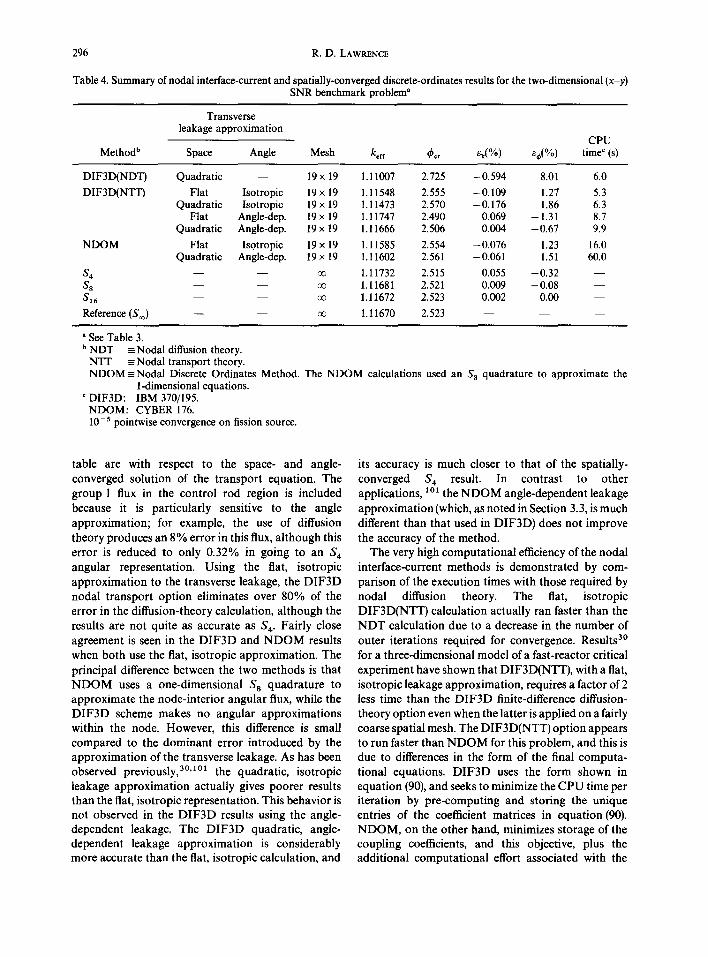
296 R.D. LAWRENCE

Table 4. Summary of nodal interface-current and spatially-converged discrete-ordinates results for the two-dimensional (x-y) SNR benchmark problem a

Transverse leakage approximation

CPU Method b Space Angle Mesh kerf ~bcr ek(%) e~(%) time c (s)

DIF3D(NDT) Quadratic

DIF3D(NTT) Flat Quadratic

Flat Quadratic

NDOM Flat Quadratic

s, $8 S16 Reference (S~)

- - 19 x 19 1.11007 2.725 -0.594 8.01 6.0

Isotropic 19 x 19 1.11548 2.555 -0.109 1.27 5.3 Isotropic 19 x 19 1.11473 2.570 -0.176 1.86 6.3

Angle-dep. 19×19 1.11747 2.490 0.069 -1.31 8.7 Angle-dep. 19 x 19 1.11666 2.506 0.004 -0.67 9.9

Is0tropic 19 × 19 1.11585 2.554 -0.076 1.23 16.0 Angle-dep. 19 x 19 1.11602 2.561 -0.061 1.51 60.0

- - oo 1.11732 2.515 0.055 -0.32 - - - - ~ 1.11681 2.521 0.009 -0.08 - - - - oo 1.11672 2.523 0.002 0.00 - -

- - oo 1.11670 2.523 - - - - - -

a See Table 3. b NDT =- Nodal diffusion theory.

NTT =Nodal transport theory. NDOM =Nodal Discrete Ordinates Method. The NDOM calculations used an S s quadrature to approximate the

t-dimensional equations. c DIF3D: IBM 370/195.

NDOM: CYBER 176. 10-5 pointwise convergence on fission source.

table are with respect to the space- and angle- converged solution of the transport equation. The group 1 flux in the control rod region is included because it is particularly sensitive to the angle approximation; for example, the use of diffusion theory produces an 8% error in this flux, although this error is reduced to only 0.32% in going to an S 4 angular representation. Using the fiat, isotropic approximation to the transverse leakage, the D I F 3 D nodal transport option eliminates over 80% of the error in the diffusion-theory calculation, although the results are not quite as accurate as S 4. Fairly close agreement is seen in the D I F 3 D and N D O M results when both use the fiat, isotropic approximation. The principal difference between the two methods is that N D O M uses a one-dimensional S s quadrature to approximate the node-interior angular flux, while the D I F 3 D scheme makes no angular approximations within the node. However, this difference is small compared to the dominant error introduced by the approximation of the transverse leakage. As has been observed previously, 3°'~°~ the quadratic, isotropic leakage approximation actually gives poorer results than the flat, isotropic representation. This behavior is not observed in the D I F 3 D results using the angle- dependent leakage, The D I F 3 D quadratic, angle- dependent leakage approximation is considerably more accurate than the fiat, isotropic calculation, and

its accuracy is much closer to that of the spatially- converged S 4 result. In contrast to other applications, 1 o 1 the N D O M angle-dependent leakage approximation (which, as noted in Section 3.3, is much different than that used in DIF3D) does not improve the accuracy of the method.

The very high computational efficiency of the nodal interface-current methods is demonstrated by comparison of the execution times with those required by nodal diffusion theory. The fiat, isotropic DIF3D(NTT) calculation actually ran faster than the N D T calculation due to a decrease in the number of outer iterations required for convergence. Results 3° for a three-dimensional model of a fast-reactor critical experiment have shown that DIF3D(NTT), with a fiat, isotropic leakage approximation, requires a factor of 2 less time than the D I F 3 D finite-difference diffusion- theory option even when the latter is applied on a fairly coarse spatial mesh. The DIF3D(NTT) option appears to run faster than N D O M for this problem, and this is due to differences in the form of the final computational equations. D I F 3 D uses the form shown in equation (90), and seeks to minimize the C P U time per iteration by pre-computing and storing the unique entries of the coefficient matrices in equation (90). N D O M , on the other hand, minimizes storage of the coupling coefficients, and this objective, plus the additional computational effort associated with the


use of a fine spatial mesh within the node, increases the computing time per iteration. The two strategies reflect the different intended applications of the codes: DIF3D is used primarily for the three-dimensional analysis of fast-reactor critical experiments where many nodes have the same dimensions and material compositions, while NDOM is intended primarily for LWR calculations involving large numbers of different compositions.

In order to compare the relative efficiencies of the nodal interface-current and nodal discrete-ordinates methods, it is necessary to establish an acceptable level of accuracy. The errors in the spatially-converged S n results given in Table 4 are due to the respective angular approximations, and on this basis we assume that S 4 angular accuracy is sufficient. The errors shown in Table 3 are due to the respective spatial approximations, and it is clear that the 19 × 19 LN calculation is a sufficiently accurate approximation to the S 4 equations. Therefore, under these assumptions, it is reasonable to compare the 19 × 19 LN solution with the quadratic, angle-dependent DIF3D(NTT) calculation since both give roughly the same S 4 accuracy. (One difficulty in this comparison is that the space and angle errors sometimes cancel; for example, the 38 × 38 LN calculation is a less accurate approximation to the exact transport solution than the 19× 19 LN solution.) Allowing for differences in computer speeds, it would appear that the nodal interface-current scheme is at least an order of magnitude faster than the LN scheme. This comparison hinges on the acceptability of S 4 accuracy since the angular approximations made in DIF3D(NTT) and NDOM limit the accuracy to about this level. (Of course, improved accuracy could be obtained at increased cost using higher-order angular representations, lo3) Furthermore, this problem is characterized by high scattering ratios (>0.9 in all groups except group 1), and this poses a severe (but still realistic) test of discrete-ordinates methods such as TWOTRAN and TWOTRAN(NODAL) which do not use diffusion-synthetic acceleration. Thus, within the framework discussed here, the nodal interface current approach offers a definite advantage in computational efficiency, but this advantage may be less pronounced in problems where transport effects are more important.

3.5. Summary and conclusions

It is appropriate that we close this section with a brief discussion of the relative advantages of the two classes of nodal transport methods discussed here. Two important advantages of the nodal discrete-

ordinates methods are (i) convergence to the exact solution of the multidimensional discrete-ordinates equations in the limit of infinitely-fine spatial mesh, and (ii) the straightforward incorporation of anisotropic scattering. The nodal interface-current methods offer the following advantages: (i) at present, they require significantly less computer time than the nodal discrete-ordinates methods, and (ii) they are less susceptible to ray effects 76 introduced by the discrete- ordinates approximation. Obvious directions for future work are suggested by the principal short- comings of each formulation. For the nodal discrete- ordinates methods, the slow iterative convergence for problems with high scattering ratios requires the further development of effective diffusion-synthetic acceleration techniques along the lines of those proposed in Refs 97 and 98. The high computational efficiency of the nodal interface-current methods is impressive, but further improvements in the angular approximations (perhaps along the lines of Ref. 103) and possibly the incorporation of anisotropic scattering are needed in order to take full advantage of this computational speed.

4. OVERVIEW

Given the high computational efficiency of present nodal diffusion methods, it is likely that future work in this area will focus more on related applications such as homogenization and dehomogenization than on new nodal procedures for solving the diffusion equation. Experience gained in the development of nodal diffusion methods has made possible the rapid extension of these ideas to the solution of the neutron transport equation. The development of effective" diffusion synthetic acceleration techniques for the nodal discrete ordinates methods is essential if these methods are to realize fully their potential for efficient three-dimensional calculations. The computational efficiency of the nodal interface-current methods is already quite high, but further improvements in the angular approximations are required for many applications of interest. Beyond these immediate needs, much exciting work remains in the development of more efficient algorithms tailored to advanced computer architectures, and in the further extension and refinement of these ideas for the solution of problems encountered in areas such as fluid flow ~°8 and charged-particle transport. 109

Acknowledgements--The author is grateful to M. R. Wagner and W. F. Walters for providing numerical results for the SNR benchmark problem. Helpful discussions with E. M. Gelbard, H, Khalil, K. S. Smith, M. R. Wagner and W. F. Waiters are acknowledged.

298 R.D. LAWRENCE

This work was supported by the United States Department of Energy while the author was in the Applied Physics Division of Argonne National Laboratory, and was com- pleted after the author joined Schlumberger-Doll Research.

REFERENCES

1. Bilodeau G. G. et al. (1957) PDQ--An IBM-704 Code to solve the two-dimensional few-group neutron diffusion equations, WAPD-TM-70, Bettis Atomic Power Labora- tory, Westinghouse Electric Corp. 2. Henry A. F. (1975) Nuclear Reactor Analysis, MIT Press, Cambridge, MA. 3. Delp D. L., Fischer D. L., Harriman J. M. and Stedwell M. J. (1964) FLARE, A three-dimensional boiling water reactor simulator, GEAP-4598, General Electric Com- pany. 4. Gupta N. K. (1981) Nodal methods for three-dimensional simulators. Prog. Nucl. Energy 7, 127. 5. Henry A. F. (1972) Refinements in accuracy of coarse- mesh finite-difference solution of the group-diffusion equations. Proc. Seminar on Numerical Reactor Calcula- tions, p. 447, Vienna, 17-21 January, International Atomic Energy Agency. 6. Wagner M. R. (1975) Current trends in multidimensional static reactor calculations. Proc. Conf. Computatio- nal Methods in Nuclear Engineering p. I-l, CONF-750413, Charleston, SC, 15-17 April, American Nuclear Society. 7. Dorning J. J. (1979) Modern coarse-mesh methods--A development of the 70's. Proc. Conf. Computational Methods in Nuclear Engineering, p. 3-1, Williamsburg, VA, 23-25 April, American Nuclear Society. 8. Smith K. S. (1986) Assembly homogenization techniques for light water reactors. Prog. Nucl. Energy 17, 303. 9. Koebke K. (1978) A new approach to homogenization and group condensation, IAEA-TECDOC-231, Inter- national Atomic Energy Agency.

10. Koebke K. (1981) Advances in homogenization and dehomogenization. Proc. Conf. Advances in Mathematical Methods for the Solution of Nuclear Engineering Problems, p. 59, Vol. II, Munich, 27-29 April, American Nuclear Society.

11. Smith K. S. (1980) Spatial homogenization methods for light water reactors, Thesis, Department of Nuclear Engineering, Mass. Inst. of Tech., Cambridge, MA.

12. Smith K. S. and Henry A. F. (1980) The determination of homogenized diffusion theory parameters for coarse mesh nodal analysis. Proc. Conf. 1980 Advances in Reactor Physics and Shielding, p. 294, Sun Valley, 14-19 Sep- tember, American Nuclear Society.

13. Finck P. J. et al. (1982) The application of nodal methods to light water reactors. Proc. Topical Meeting on Advances in Reactor Physics and Core Thermal Hydraulics, p. 348, Kiamesha Lake, New York, 22-24 September, NUREG/CP-0034, U.S. Nuclear Regulatory Commission.

14. Khalil H. S., Finck P. J. and Henry A. F. (1983) Reconstruction of pin powers from nodal results. Proc. Meeting on Advances in Reactor Computations, p. 367, Salt Lake City, 28-31 March, American Nuclear Society.

15. Koebke K., Hetzelt L., Wagner M. R. and Winter H.-J. (1984) Principles and application of advanced nodal reactor analysis methods. Proc. Topical Meeting on Reactor Physics and Shielding, p. 134, Chicago, 17-19 Sep- tember, American Nuclear Society.

16. Koebke K. and Wagner M. R. (1977) The determination of the pin power distribution in a reactor core on the basis

of nodal coarse mesh calculations. Atomkernenergie 30, 136.

17. Wagner M. R. (1974) Nodal synthesis method and imbedded flux calculations. Trans. Am. Nucl. Soc. 18, 152.

18. Antonopoulous P. T. (1972) Large mesh model development study, Thesis, Department of Nuclear Engineering, Mass. Inst. Tech., Cambridge, MA.

19. Wachspress E. L., Burgess R. D. and Baron S. (1962) Multi-channel flux synthesis. Nucl. Sci. Engr. 12, 381.

20. Bennewitz F., Finnemann H. and Moldaschl H. (1975) Solution of the multidimensional neutron diffusion equation by nodal expansion. Proc. Conf. Computational Methods in Nuclear Engineering, p. 1-99, CONF-750413, Charleston, S.C., 15-17 April, American Nuclear Society.

21. Bennewitz F., Finnemann H. and Wagner M. R. (1975) Higher-order corrections in nodal reactor calculations. Trans. Am. Nucl. Soc. 22, 250.

22. Finnemann H., Bennewitz F. and Wagner M. R. (1977) Interface current techniques for multidimensional reactor calculations. Atomkernenergie 30, 123.

23. Wagner M. R., Koebke K. and Winter H.-J. (1981) A nonlinear extension of the nodal expansion method. Proc. Conf. Advances in Mathematical Methods for the Solution of Nuclear Engineering Problems, p. 43, Vol. II, Munich, 27-29 April, American Nuclear Society.

24. Shober R. A. (1976) Nonlinear methods for solving the diffusion equation, Thesis, Department of Nuclear Engin- eering, Mass. Inst. of Tech., Cambridge, MA.

25. Shober R. A., Sims R. N. and Henry A. F. (1977) Two nodal methods for solving time-dependent group diffusion equations. Nucl. Sci. Engr. 64, 582.

26. Smith K. S. (1979) An analytic nodal method for solving the two-group, multidimensional, static and transient neutron diffusion equations. Nuc. Engr. Thesis, Depart- ment of Nuclear Engineering, Mass. Inst. of Tech., Cambridge, MA.

27. Greenman G., Smith K. S. and Henry A. F. (1979) Recent advances in an analytic nodal method for static and transient reactor analysis. Proc. Computational Methods in Nuclear Engineering, p. 3-49, Williamsburg, VA, 23-25 April, American Nuclear Society.

28. Sims R. (1977) A coarse-mesh nodal diffusion method based on response matrix considerations. Thesis, Depart- ment of Nuclear Engineering, Mass. Inst. of Tech., Cambridge, MA.

29. Maeder C. (1978) A nodal diffusion method with Legendre polynomials. Proc. Topical Meeting on Advances in Reactor Physics, p. 121, Gatlinburg, TN, 11~12 April, American Nuclear Society.

30. Lawrence R. D. (1984) Three-dimensional nodal diffusion and transport methods for the analysis of fast-reactor critical experiments. Proc. Topical Meeting on Reactor Physics and Shielding, p. 814, Chicago, 17-19 September, American Nuclear Society. See also: Lawrence R. D. (1986) Prog. Nucl. Energy, to appear.

31. Lawrence R. D. (1979) A nodal Green's function method for multidimensional neutron diffusion calculations. Thesis, Nuclear Engineering Program, Univ. of Illinois, Urbana.

32. Lawrence R. D. and Dorning J. J. 0980) A nodal Green's function method for multidimensional neutron diffusion calculations. Nucl. Sci. Engr. 76, 218.

33. Shober R. A. (1979) A nodal method for fast reactor analysis. Proc. Computational Methods in Nuclear Engin- eering, p. 3-33, Williamsburg, VA, 23-25 April, American Nuclear Society.


34. Birkhofer A. and Werner W. (1973) Efficiency of various methods for the analysis of space-time kinetics. Proc. Conf. Mathematical Models and Computational Techniques for Analysis of Nuclear Systems, Vol. II, p. IX-31, CONF730414, Ann Arbor, MI, 9-11 April, American Nuclear Society.

35. Langenbuch S., Maurer W. and Werner W. (1977) Coarse-mesh flux expansion method for the analysis of space-time effects in large light water reactor cores. Nucl. Sci. Engr. 63, 437.

36. Langenbuch S., Maurer W. and Werner W. (1977) High-order schemes for neutron kinetics calculations, based on a local polynomial approximation. Nucl. Sci. Engr. 64, 508.

37. Rydin R. A. and Sullivan T. M. (1978) A new approach to the QUABOX-CUBBOX coarse-mesh methods. Proc. Topical Meeting on Advances in Reactor Physics, p. 131, Gatlinburg, TN, 10-12 April, American Nuclear Society.

38. Rydin R. A., Robinson M. A. and Wantuck P. J. (1979) Recent advances in the QUAD and CUBE coarse-mesh diffusion theory methods. Proc. Conf. Computational Methods in Nuclear Engineering, p. 3 73, Williamsburg, VA, 23-25 April, American Nuclear Society.

39. Dilber I. and Lewis E. E. (1984) Two-dimensional variational coarse-mesh methods. Proc. Topical Meeting on Reactor Physics and Shielding, p. 149, Chicago, 17-19 September, American Nuclear Society.

40. Bonalumi R. A. et al. (1978) MUSIC--A Mesh- Unrestricted Simulation Code. Proc. Topical Meeting on Advances in Reactor Physics, p. 169, Gatlinburg, TN, 10-12 April, American Nuclear Society.

4t. Melice M. (1978) A nodal-modal coarse-mesh method for solving the few-group diffusion equation. NEACRP-L-228, Elektrobel, Brussels.

42. Arkuszewski J. J. and Makai M. (1981) Analytic coarse- mesh approximations for solving diffusion equations in hexagonal and square geometries. Proc. Conf. Advances in Mathematical Models for the Solution of Nuclear Engin- eering Problems, p. 75, Vol. II, Munich, 27 29 April, American Nuclear Society.

43. Makai M. and Maeder C. (1983) A fast nodal neutron diffusion method for cartesian geometry. Nucl. Sci. Engr. 84, 390.

44. Burns T. J. (1975) The partial current balance method: a local Green's function technique for the numerical solution of multidimensional neutron diffusion problems. Thesis, Nuclear Engineering Program, Univ. of Illinois, Urbana.

45. Burns T. J. and Doming J. J. (1975) Multidimensional applications of an integral balance technique for neutron diffusion computations. Proc. Conf. Computational Meth- ods in Nuclear Engineering, p. V-57, CONF-750413, Char- leston, SC, 15-17 April, American Nuclear Society.

46. Kaloinen E., Siltanen P. and Terasvirta R. (1979)Two- group nodal calculations in hexagonal fuel assembly geometry. Proc. Specialists' Meetin 9 on Calculation of Three-Dimensional Rating Distributions in Operating Reac- tors, p. 111, Paris, 26--28 November, OECD, Paris.

47. Duracz T. (1981) A nodal method in hexagonal geometry. Proc. Conf. Advances in Mathematical Methods .for the Solution of Nuclear Engineering Problems, p. 423, Vol. I, Munich, 27-29 April, American Nuclear Society.

48. Lawrence R. D. (1981) A nodal interface current method for multigroup diffusion calculations in hexagonal geometry. Trans. Am. Nucl. Soc. 39, 461.

49. Lawrence R. D. (1983) A nodal method for three- dimensional fast reactor calculations in hexagonal geo-

metry. Proc. Conf. Advances in Reactor Computations, p. 1030, Vol. II, Salt Lake City, UT, 28-31 March, American Nuclear Society.

50. Makai M. and Arkuszewski, J. (1981) A hexagonal coarse-mesh program based on symmetry considerations. Trans. Am. Nucl. Soc. 38, 347.

51. Askew J. R. et al. (1972) Methods for three-dimensional fuel management studies on high temperature reactors. Proc. Conf. New Developments in Reactor Physics and Shielding, CONF-720901, p. 68, Book 1, Kiamesha Lake, NY, 12-15 September, American Nuclear Society.

52. Dodds H. L., Honeck H, C. and Hostetler D. E. (1977) A coarse-mesh method for multidimensional, mixed-lattice diffusion calculations. Nucl. Sci. Engr. 62, 751.

53. Takeda T. et al. (1979) Effective one-group coarse-mesh method for calculating three-dimensional power distribution in fast reactors. Annals Nucl. Energy 6, 65.

54. Lukas H. and Wehmann U. (1981) A fast two- and three-dimensional one group coarse-mesh diffusion program in hexagonal geometry. Proc. Conf. Advances in Mathematical Methods for the Solution of Nuclear Engin- eering Problems, p. 299, Vol. I, Munich, 27-29 April, America Nuclear Society.

55. Ferguson D. R. and Derstine K. L. (1977) Optimized iteration strategies and data management considerations for fast reactor finite difference diffusion theory codes. Nucl. Sci. Engr. 64, 593.

56. Wachspress E. L. (1966) Iterative solution of elliptic systems. Prentice-Hall Inc., Englewood Cliffs, NJ.

57. Froehlich R. (1967) A theoretical foundation for coarse- mesh variational techniques. GA-7870, Gulf General Atomic.

58. Wagner M. R. (1968) GAUGE: A two-dimensional few group neutron diffusion-depletion for a uniform triangular mesh. GA-8307, Gulf General Atomic.

59. Wagner M. R. and Koebke K. (1983) Progress in nodal reactor analysis. Proc. Conf. Advances in Reactor Compu- tations, p. 941, 28-31 March, Salt Lake City, UT, Ameri- can Nuclear Society.

60. Koebke K. (1984) Private Communication. 61. Smith K. S. (1983) Nodal method storage reduction by

nonlinear iteration. Trans. Am. Nucl. Soc. 44, 265. 62. Argonne Code Center: Benchmark Problem Book

(1977) ANL-7416, Suppl. 2, Argonne National Labora- tory. Descriptions of the IAEA benchmark problem also appear in Refs 6 and 43.

63. Wagner M. R., Finnemann H., Koebke K. and Winter H.-J. (1977) Validation of the nodal expansion method and the depletion program MEDIUM-2 by benchmark calculation and direct comparison with experiment. Atomkerne- nergie 30, 129.

64. Vondy D. R., Fowler T. B. and Cunningham G. W. (1975) VENTURE: A code block for solving multigroup neutronics problems applying the finite-difference diffusion-theory approximation to neutron transport. ORNL-5062, Oak Ridge National Laboratory.

65. Derstine K. L. (1984) DIF3D: A code to solve one-, two- and three-dimensional finite-difference diffusion theory problems. ANL-82-64, Argonne National Laboratory.

66. Maeder C., et al. (1979) Calculations with the EIR light water reactor code system. Proc. Specialists' Meeting on Calculation of Three-Dimensional Rating Distributions in Operating Reactors, p. 181, Paris, 26-28 November, OECD, Paris.

67. Buckel G,, Kufner K. and Stehle B. (1977) Benchmark calculations for a sodium-cooled breeder reactor by two-

300 R.D. LAWRENCE

and three-dimensional diffusion methods. Nucl. Sci. Engr. 6,1, 75.

68. Benchmark Problem Book (1986) ANL-7416, Supple. 3, Argonne National Laboratory, to appear.

69. Lawrence R. D. (1983) The DIF3D nodal neutronics option for two- and three-dimensional diffusion theory calculations in hexagonal geometry. ANL-83-1, Argonne National Laboratory.

70. Werner W., Finnemann H. and Langenbuch S: (1976) Two- and three-dimensional BWR kinetics benchmark problems. Trans. Am. Nucl. Soc. 23, 215.

71. Bowring R. W., Stewart J. W., Shober R. A. and Sims R. N. (1975) MEKIN: MIT-EPRI nuclear reactor core kinetics code. EPRI-227, Electric Power Research Insti- tute.

72 Meneley D. A. et al. (1972) A kinetics model for fast reactor analysis in two dimensions. In: Dynamics of Nuclear Systems, p. 483 (Hetrick D. L. ed.), The University of Arizona Press, Tucson.

73. Lawrence R. D. (1984) Perturbation theory within the framework of a higher-order nodal method. Trans. Am. Nucl. Soc. 46, 402.

74. Taiwo T. A. and Henry A. F. (1985) Perturbation theory based on a nodal model. Proc. International Meeting on Advances in Nuclear Engineering Computational Methods, p. 527, Vol. II, Knoxsville, TN, 9-11 April, American Nuclear Society.

75. Hoxie C. L. (1985) A nonlinear coupling coefficient iteration for solving the nodal three-dimensional transient diffusion equation. Proc. International Meeting on Advances in Nuclear Engineering Computational Methods, p. 595, Vol. II, Knoxsville, TN, 9-11 April, American Nuclear Society.

76. Lewis E. E. and Miller W. F. (1984) Computational Methods of Neutron Transport, John Wiley and Sons, New York.

77. Lawrence R. D. and Doming J. J. (1979) New coarse- mesh diffusion and transport theory methods for the efficient numerical calculation of multi-dimensional reactor power distributions. Proc. Spec. Meeting on the Calculation of Three-Dimensional Rating Distributions in Operating Reactors, p. 383, Paris, 26-28 November, NEACRP/OECD.

78. Doming J. J., Lawrence R. D. and Ougouag A. M. (1979) application of a new coarse-mesh computational method to the determination of power distributions in a heterogeneous-core large fast reactor. Proc. IAEA Sym- posium Fast Reactor Physics, p. 383, Aix-en-Provence, 24--28 September, IAEA, Vienna.

79. Lawrence R. D. and Doming J. J. (1980) A discrete nodal integral transport theory method for multidimensional reactor physics and shielding calculations. Proc. Conf. 1980 Advances in Reactor Physics and Shielding, p. 840, Sun Valley, ID, 14-19 September, American Nuclear Society.

80. Waiters W. F. and O'Dell R. D. (1980) Nodal methods for discrete-ordinates transport problems in (x-y) geometry. Proc. Conf. Advances in Mathematical Methods for the Solution of Nuclear Engineering Problems, p. 115, Vol. I, Munich, 27-29 April, American Nuclear Society.

81. Waiters W. F. and O'Dell R. D. (1981) A comparison of linear nodal, linear discontinuous, and diamond schemes for solving the transport equation in (x, y) geometry. Trans. Am. Nucl. Soc. 39, 465. See also: Waiters W. F. (1982) Recent developments in nodal and characteristic methods in transport theory. Trans. Am. Nucl. Soc. 43, 611.

82. Waiters W. F. (1985) Augmented weighted diamond form of the linear nodal scheme for cartesian coordinate systems. Proc. International Meeting on Advances in Nuclear Engineering Computational Methods, p. 452, Vol. II, Knoxville, TN, 9-11 April, American Nuclear Society.

83. Pevey R. E. (1982) Development of a new two- dimensional cartesian geometry nodal multigroup discrete ordinates method. ORNL/CSD/TM-182, Oak Ridge National Laboratory.

84. Pevey R. E. and Dodds H. L (1981) A two-dimensional exponential expansion discrete-ordinates nodal method. Trans. Am. Nucl. Soc. 39, 751.

85. Ullo J. J., Doming J. J., Dodds H. L. and Pevey R. E. (1982) A comparison of nodal transport methods based on exponential and polynomial expansions. Trans. Am. Nucl. Soc. 43, 367.

86. Ullo J. J. (1985) Private communication. 87. Badruzzaman A. and Xie Zhong-Zeng (1984) A three-

dimensional linear nodal transport method. Trans. Am. Nucl. Soc. 47, 223. See also: Badruzzaman A. et al. (1985) A discrete nodal transport method for three-dimensional reactor physics and shielding calculations. Proc. Topical Meeting on Reactor Physics and Shielding, p. 170, Chicago, 17-19 September, American Nuclear Society.

88. Badruzzaman A. (1985) An efficient algorithm for nodal transport solutions in multidimensional geometry. Nucl. Sci. Engr. 89, 281.

89. Alcouffe R. E. and Larsen E. W. (1981) A review of characteristic methods used to solve the linear transport equation. Proc. Conf. Advances in Mathematical Methods for the Solution of Nuclear Engineering Problems, p. 3, Vol. I, Munich, 27-29 April, American Nuclear Society.

90. Larsen E. W. and Alcouffe R. E. (1981) The linear characteristic method for spatially discretizing the discrete ordinates equations in (x, y) geometry. Proc. Conf. Advances in Mathematical Methods for the Solution of Nuclear Engineering Problems, p. 99, Vol. I, Munich, 27-29 April, American Nuclear Society.

91. Beernick K. P. and Doming J. J. (1983) The relationships between the nodal, and moments characteristic, transport methods and their errors. Proc. Conf. Advances in Reactor Computations, p. 737, Vol. II, Salt Lake City, UT, 28-31 March, American Nuclear Society.

92. Waiters W. F. (1983) The TLC scheme for numerical solution of the transport equation on equilateral triangular meshes. Proc. Conf. Advances in Reactor Computations, p. 151, Vol. I, Salt Lake City, UT, 28-31 March, American Nuclear Society.

93. Paternoster R. R. and Waiters W. F. (1984) A linear characteristic-nodal transport method for arbitrary triangular meshes in (x, y) Geometry. Trans. Am. Nucl. Soc. 46, 431.

94. Sanchez R. and McCormack N. J. (1982) A review of transport approximations. Nucl. Sci. Engr. 811, 481.

95. Alcouffe R. E. (1977) Diffusion synthetic acceleration methods for the diamond-differenced discrete-ordinates equations. Nucl. Sci. Engr. 64, 344.

96. Larsen E. W. (1983) Diffusion-synthetic acceleration methods for the discrete-ordinates equations. Proc. Conf. Advances in Reactor Computations, p. 705, Vol. II, Salt Lake City, UT, 28-31 March, American Nuclear Society.

97. Khalil H. (1985) A nodal diffusion technique for synthetic acceleration of nodal 5', calculations. Nucl. Sci. Engr. 9@, 263.

98. Azmy Y. Y. and Doming J. J. (1985) Diffusion synthetic


acceleration of the multidimensional discrete nodal transport method. Pro~. International Meeting on Advances in Nuclear Engineering Computational Methods, p. 440, Vol. II, Knoxsville, TN, 9-11 April, American Nuclear Society.

99. Mohanakrishnan P. (1981) Angular current approximations in neutron transport calculations using interface currents--a review. Prog. Nucl. Energy 7, 1.

100. Wagner M. R. (1979) A nodal discrete-ordinates method for the numerical solution of the multidimensional transport equation. Proc. Conf. Computational Methods in Nuclear Engineering, p. 4-117, Williamsburg, VA, 23 25 April, American Nuclear Society.

101. Wagner M. R. and Muller B. (1984) The nodal discrete ordinates method and its application to LWR lattice problems. Proc. Topical Meeting on Reactor Physics and Shielding, p. 376, Chicago, 17-19 September, American Nuclear Society.

102. Gelbard E. M. (1985) Model problem study of transverse-leakage treatment in nodal transport methods. Trans. Am. Nucl. Soc. 49, 214.

103. Stepanek J. (1981) The DPN and QPN surface flux integral transport methods in one-dimensional geometries and x ~ geometry. Proc. Conf. Advances in Mathematical Methods for the Solution of Nuclear Engineering Problems,

p. 51, Vol. I, Munich, 27 29 April, American Nuclear Society.

104. O'Dell R. D., Stepanek J. and Wagner M. R. (1983) Intercomparison of the finite difference and nodal discrete ordinates and surface flux transport methods for a LWR pool reactor benchmark problem in x y geometry. Proc. Conf. Advances in Reactor Computations, p. 757, Vol. II, Salt Lake City, UT, 28 31 March, American Nuclear Society.

105. The TWOTRAN and TWOTRAN(NODAL) results, plus the TWODANT CPU times for the CRAY-I, were provided by W. F. Waiters.

106. Lathrop K. D. and Brinkley F. W. Jr. (1973) TWOTRAN-II: An interfaced exportable version of the TWOTRAN code for two-dimensional transport. LA-4848-MS, Los Alamos National Laboratory.

107. Alcouffe R. E., et al. (1984) User's guide for TWO- DANT. LA-10049-M, Los Alamos National Laboratory.

108. For example, see: Azmy Y. Y. and Dorning J. J. (1983) A nodal integral approach to the numerical solution of partial differential equations. Proc. Conf. Advances in Reactor Computations, p. 893, Vol. II, Salt Lake City, UT, 28 31 March, American Nuclear Society.

109. Waiters W. F. (1985) Private communication.

progress in nodal methods for the solution …li.mit.edu/stuff/cnse/paper/lawrence86pne.pdf · 272...

Documents