Progress in Computational Complexity Theory

Jin-Yi Cai ∗

Computer Sciences Department

University of Wisconsin

Madison, WI 53706. USA.

Email: jyc@cs.wisc.edu

and

Tsinghua University

Beijing, China

Hong Zhu†

Computer Sciences Department,

Fudan University

Shanghai 200433, China.

Email: hzhu@fudan.edu.cn

Abstract

We briefly survey a number of important recent achievements in Theoretical Computer Sci-ence (TCS), especially Computational Complexity Theory. We will discuss the PCP Theorem,its implications to inapproximability on combinatorial optimization problems; space boundedcomputations, especially deterministic logspace algorithm for undirected graph connectivityproblem; deterministic polynomial-time primality test; lattice complexity, worst-case to average-case reductions; pseudorandomness and extractor constructions; and Valiant’s new theory ofholographic algorithms and reductions.

Key words: Theoretical Computer Science, Computational Complexity Theory, PCP Theo-rem, Inapproximability, Logspace complexity, Reingold’s Theorem, GAP problem, Primality test-ing, Complexity of lattice problems, Worst-case to average-case reductions, Pseudorandomness,Extractors, Holographic algorithms.

1 Background

The field of Theoretical Computer Science (TCS), especially Computational Complexity Theory, isarguably the most foundational aspect of Computer Science. It deals with fundamental questionssuch as, what is feasible computation, and what can and cannot be computed with a reasonableamount of computational resources in terms of time and/or space. It offers new and profound insightinto concepts which have fascinated mankind for generations—proof and verification, randomness,efficiency, security, and of course computation.

This field is also one of the most vibrant. A great deal of fascinating research is being conductedwith ever more sophisticated mathematical techniques. The results are deep, elegant and surprising.In this brief survey of some recent striking developments, we wish to sample a few of the highlights,to give the reader a flavor of this great achievement. We decided not to write something likean “executive survey” which only scratches the surface with some vague generalities. Instead wedecided to delve deeper, to offer a glimpse of the true frontier as an active researcher sees it. Andwhat a glorious frontier it is! We hope the earnest reader will come away with a new appreciation

∗Supported by an NSF Grant, USA (CCR-0208013 and CCR-0511679).†Supported by a grant from National Natural Science Fund grant #60496321

1

of this great intellectual edifice that is being built called Computational Complexity Theory. Andif some young reader finds this subject so attractive as to devote himself in the study, we will feelamply rewarded.

With such a short survey, it is impossible to do justice to all the interesting and important topicsin Complexity Theory. And in order to discuss some topics with a certain depth, it is necessary tochoose only a small number of topics. We made this choice based on personal taste. This reflectsthe limitations of the authors, both in their insight as well as in their knowledge. We also apologizebeforehand for any errors.

We assume the readers are acquainted with a basic knowledge of Theoretical Computer Science,such as the notion of computability (by Turing machines), time and space bounded computationsand their respective hierarchy theorems, polynomial time reductions and NP-completeness theory.In short we assume the readers are familiar with the theory of computing at the level of knowledgerepresented by [21, 30].

The reader is likely to have also known some more recent developments such as a) the use ofrandomness in computation, b) randomized complexity classes, c) pseudorandomness as rigorouslyformulated by Blum-Micali [12] and Yao [73], as being indistinguishable from true randomness byany bounded computations such as polynomial time, and d) interactive proof systems.

2 The PCP Theorem

We speak of a computational task being “easy” if it can be accomplished by a Turing machinein polynomial time. This is the class P. The complexity class NP [19] was first defined as a proofsystem where a true statement can be easily certified to be so, while the system does not erroneouslyaccept any false statement. E.g., consider the claim that a boolean formula ϕ is satisfiable. If ϕ issatisfiable, then this claim can be easily certified to be so by any satisfying assignment to ϕ. If ϕis not satisfiable, then no purported satisfying assignment can convince us that ϕ is satisfiable.

Interactive Proof (IP) systems were proposed by Goldwasser, Micali and Rackoff in [27] as aprobabilistic and interactive version of NP which is capable of proving an (apparently) wider classof statements. In such a system a Prover P is computationally unrestricted (called all powerful—logically, this means that his moves are existential) which interacts with a computationally restrictedVerifier V (usually by probabilistic polynomial time). It is required that, when statement ϕ is truethen P can convince V of its truth after a sequence of interactions. (This is called completenessrequirement. In Logic, a proof system that can prove all true statements within the system iscalled complete.) Because V is polynomially bounded this sequence of interactions is, of necessity,also polynomially bounded. However, in this sequence of interactions the verifier V can also userandom moves. For an IP system it is also required that when a statement is false, then anydishonest prover P ′ can not convince our verifier V that ϕ is true, with probability > 1%, say.(This is called soundness requirement. In Logic, a proof system that only proves true statementswithin the system is called sound. Here 1% can be easily made exponentially small by a polynomialnumber of repetitions of the protocol.)

Here is an example of an IP system. It is for graph non-isomorphism (GNI). Clearly graphisomorphism (GI) is in NP: To prove two graphs are isomorphic, one only need to exhibit anisomorphism, which can be easily checked. However, it is not clear there is any universal propertywhich proves two graphs are non-isomorphic and can be checked in polynomial time. Listing allpossible maps and then verify that none is an isomorphism takes exponential time. Therefore GNIis not known to be in NP. However, consider the following game: A prover P claims that twolabeled graphs A and B are non-isomorphic, and invites any verifier V to pick one of them in

2

secret. Then V can apply a secret permutation to its vertices and present the resulting graph Gback to P , and challenge P to identify which one of A and B was picked by V . V will acceptP ’s claim of non-isomorphism iff P answers this challenge correctly. Note that if A and B arenot isomorphic then the permuted graph G is isomorphic to exactly one of A and B, and P cansucceed in this case. However, If A and B are isomorphic, and V chooses among A and B withequal probability and then applies a uniformly chosen permutation, then his graph G is a uniformsample from all graphs isomorphic to both A and B. Hence no cheating prover P ′ can meet thechallenge with success probability greater than 1/2. n parallel iterations (where they play this gameindependently in parallel n times, and V accepts iff all the answers P gives are correct) reduce thesuccess probability of any cheating prover down to 1/2n.

It might appear that the use of secrecy in the random choice by V was essential. Independently,Babai [9] (see also [10]) proposed a public coin version of IP system called Arthur-Merlin games.Here the prover is called Merlin, and he can see all the coin flips the verifier (Arthur) makes. Itwas quite a surprise that Goldwasser and Sipser [28] showed that these two versions of IP systemsare equivalent in computational power.

One interesting consequence of the fact that GNI having a constant round IP protocol is thatGI is not NP-complete, unless the Polynomial Hierarchy PH collapses. Whether GI is NP-completehas been an open problem since the original paper on NP-completeness by Karp [33].

There followed a remarkable sequence of development in TCS starting in the late 80’s andearly 90’s that eventually led to the celebrated PCP Theorem. Lund, Fortnow, Karloff and Nisan[42], following an initial breakthrough by Nisan, first showed that the permanent function Permhas an IP system. Perm is known to be hard for NP, in fact #P-hard, and thus hard for theentire Polynomial-time Hierarchy PH. Shortly afterwards A. Shamir [60] proved that the class ofproperties provable by IP is exactly the class PSPACE, the problems solvable in polynomial space.

The concept of Multiprover Interactive Proof (MIP) system [11] was introduced sometime afterIP systems, and was apparently for purely intellectual purposes, with no practical applicationsin mind. After Shamir’s result of IP = PSPACE, the power of MIP was also characterized asNEXP, non-deterministic exponential time. More importantly, the MIP concept eventually led tothe concept of Probabilistically Checkable Proofs (PCP).

The next breakthrough came in a 1991 paper by Feige, Goldwasser, Lovasz, Safra, and Szegedy[24]. In this paper, they first established a close relationship between the approximability of MAX-CLIQUE problem and two prover interactive proof systems. In very rough terms, the “proofs” theprovers offer become vertices and their mutual consistencies become edges in a certain graph onwhich, either there is a large clique (a copy of the complete graph Km) or there are only smallcliques. This becomes a reduction, so that, in essence, one can reduce a decision problem to a gapproblem (here the gap problem refers to the gap in the clique size, which is either small or large.)Thus any approximation algorithm with a performance guarantee within that gap translates intoa decision algorithm for the original decision problem.

Many rounds of improvements eventually culminated in the following PCP Theorem.

Theorem 2.1 (Arora, Lund, Motwani, Sudan, Szegedy) Fix any ǫ > 0. Every set S ∈ NPhas a proof scheme as follows: There is a polynomial time proof checker C which can flip coins,such that

• ∀x ∈ S, there exists a “short proof” y, C will accept x with probability 1 after it examines aconstant number of randomly chosen bits of y.

• ∀x 6∈ S, for any purported “short proof” y, C will reject x with probability ≥ 1 − ǫ after itexamines a constant number of randomly chosen bits of y.

3

Building on this result, a great many inapproximability results followed, including MAXSAT,MAXCUT, Clique, Vertex Cover etc. E.g., it is shown that approximating Clique size to n1−ǫ forany ǫ > 0 is NP-hard. Research has since moved ahead with tremendous vigor. Today, the knownresults are quite amazingly broad and strong, and research is still advancing rapidly.

The interested reader can find much more information and many interesting pointers at thefollowing web pagehttp://www-cse.ucsd.edu/users/~mihir/pcp.html

3 Reingold’s Theorem

Space bounded computation is only second in importance to time bounded computations. Themodel of space bounded computation is an off-line Turing machine where the input tape is readonly (size n) and does not count toward its space complexity. The space complexity is measured bythe usage of the off-line read/write work tape. This way one can discuss sublinear o(n) space com-plexity, in particular O(log n) or (log n)O(1) bounded computations, which turn out to be extremelyimportant and interesting.

Clearly both deterministic logspace L (= DSAPCE[O(log n)]) and non-deterministic logspaceNL (= NSAPCE[O(log n)]) are subclasses of P. NL is represented, and in a technical sense in anessential way, by the following concrete problem called GAP (Graph Accessibility Problem): Givena directed graph G, and two vertices s and t, is there a directed path from s to t? Clearly onecan solve GAP by Depth-First-Search, which takes linear time but it also takes linear space. Non-deterministically one can guess a path step by step, only remembering the current vertex visited.The question is can one do better deterministically in terms of space complexity?

Savitch [59] gave a recursive algorithm which solves GAP in space O((log n)2). Unfortunatelythe time complexity is super-polynomial nO(log n).

Major progress has been made for undirected graphs: Given an undirected graph G, is Gconnected? This problem is usually phrased as follows, and called USTCON: Given an undirectedgraph G and two vertices s and t, is there a path from s to t in G?

The first truly beautiful result on this problem is due to Aleliunas,, Karp, Lipton, Lovasz andRackoff [7] in 1979. They showed that a random walk of length O(n3) is most likely to visit allvertices of an undirected graph, no matter what n-vertex graph it is or which vertex the walk startsat. This gives a randomized algorithm as follows: To decide if one can reach from vertex s to t,one simply starts a random walk at s of length O(n3), and check that vertex t is ever reached.The remarkable fact is that this algorithm uses only O(log n) space—essentially it only needs toremember the name of the vertex it is currently visiting.

Subsequent improvements came with attempts to derandomize this algorithm, and more gener-ally to derandomize all algorithms in randomized logspace RL or BPL. Here in analogy to random-ized polynomial time classes, we define RL to consist of languages L acceptable by probabilisticlogspace Turing Machines M such that whenever x ∈ L then Pr[M(x) = 1] ≥ 1/2 and for x 6∈ L,Pr[M(x) = 1] = 0. Here the probability Pr is taken over a sequence of polynomially many randombits, which the logspace Turing Machine M can access only on a one-way read-only tape. Machinesaccepting languages in RL have only one-sided error (when x ∈ L). BPL is the same except weallow two-sided error.

Nisan in 1992 [48] gave a pseudorandom generator which uses seed length O((log n)2) andproduces a polynomially long sequence of pseudorandom bits provably indistinguishable by anylogspace bounded computation. While it did not improve the space bound of Savitch directly,Nisan showed that his generator can be used to prove an interesting result: The undirected graph

4

( u, a ) u, a’)(

( v, b’) ( v, b)

Gu

v

a’

H

a’

H

H

u

v

x x’x x’

y y’

y y’

a

b’ bb’

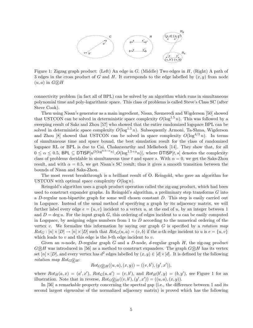
Figure 1: Zigzag graph product: (Left) An edge in G, (Middle) Two edges in H, (Right) A path of3 edges in the cross product of G and H. It corresponds to the edge labelled by (x, y) from node(u, a) in G z©H

connectivity problem (in fact all of BPL) can be solved by an algorithm which runs in simultaneouspolynomial time and poly-logarithmic space. This class of problems is called Steve’s Class SC (afterSteve Cook).

Then using Nisan’s generator as a main ingredient, Nisan, Szemeredi and Wigderson [50] showedthat USTCON can be solved in deterministic space complexity O(log1.5 n). This was followed by asweeping result of Saks and Zhou [57] who showed that the entire randomized logspace BPL can besolved in deterministic space complexity O(log1.5 n). Subsequently Armoni, Ta-Shma, Wigdersonand Zhou [8] showed that USTCON can be solved in space complexity O(log4/3 n). In termsof simultaneous time and space bound, the best simulation result for the class of randomizedlogspace RL or BPL is due to Cai, Chakaravarthy and Melkebeek [14]. They show that, for all

0 ≤ α ≤ 0.5, BPL ⊆ DTISP[nO(log0.5−αn), O(log1.5+αn)], where DTISP[t, s] denotes the complexityclass of problems decidable in simultaneous time t and space s. With α = 0, we get the Saks-Zhouresult, and with α = 0.5, we get Nisan’s SC result; thus it gives a smooth transition between thebounds of Nisan and Saks-Zhou.

The most recent breakthrough is a brilliant result of O. Reingold, who gave an algorithm forUSTCON with optimal space complexity O(log n).

Reingold’s algorithm uses a graph product operation called the zig-zag product, which had beenused to construct expander graphs. In Reingold’s algorithm, a preliminary step transforms G intoa D-regular non-bipartite graph for some well chosen constant D. This step is easily carried outin Logspace. Instead of the usual method of specifying a graph by its adjacency matrix, we willfurther label every edge e = u, v incident to a vertex u, at the end of u, by an integer between 1and D = deg u. For the input graph G, this ordering of edges incident to u can be easily computedin Logspace, by assigning edges numbers from 1 to D according to the numerical ordering of thevertex v. We formalize this information by saying our graph G is specified by a rotation mapRotG : [n]× [D] → [n]× [D] such that RotG(u, a) = (v, b) if the a-th edge incident to u is e = u, vwhich leads to v and this edge is the b-th edge incident to v.

Given an n-node, D-regular graph G and a D-node, d-regular graph H, the zig-zag productG z©H was introduced in [56] as a method to construct expanders. The graph G z©H has its vertexset [n]×[D], and every vertex has d2 edges labelled by (x, y) ∈ [d]×[d]. It is defined by the followingrotation map RotG z©H :

RotG z©H((u, a), (x, y)) = ((v, b′), (y′, x′)),

where RotH(a, x) = (a′, x′), RotG(u, a′) = (v, b′), and RotH(b′, y) = (b, y′), see Figure 1 for anillustration. Note that in reverse, RotG z©H((v, b′), (y′, x′)) = ((u, a), (x, y)).

In [56] a remarkable property concerning the spectral gap (i.e., the difference between 1 and itssecond largest eigenvalue of the normalized adjacency matrix) is proved which has the following

5

direct consequence [55]:

1 − λ(G z©H) ≥ 1

2(1 − λ(H)2)(1 − λ(G))

where λ(X) denotes the second largest eigenvalue of the normalized adjacency matrix of graphX. Essentially this shows that if H is chosen to be a good expander (i.e., a graph with a smallsecond largest eigenvalue), then G z©H will have a spectral gap not much smaller than that of G.Meanwhile a powering of X will increase the spectral gap of X, since λ(Xk) = (λ(X))k . Reingoldchose D = d16 and an appropriate H with D vertices. Then (G z©H)8 is D-regular again, and hasan increased spectral gap than G by the spectral gap formula above.

The main part of Reingold’s algorithm is to repeatedly apply the zig-zag product and graphpowering to the input graph G, to obtain a G′ after O(log n) steps. G′ is connected iff G isconnected. Now each connected component of G′ is an expander with second largest eigenvalue atmost 1/2. Being an expander, this implies that any pair of nodes in the same connected componentof G′ are joined by a path of length at most O(log n). Thus, on G′, one can solve connectivityproblem in deterministic logspace.

The zig-zag product operation has turned out to be extremely powerful. It was initially usedfor the construction of explicit families of expander graphs, which is a rich subject with enormouslyimportant applications by itself. But we will not go into that in this article. There has alreadybeen some important follow ups. Dinur [23] has shown how to use a similar approach to give asimpler proof of the PCP Theorem, which has some stronger parameters.

There is at least one other important result regarding space complexity in the last twentyyears which we should mention. Immerman and Szelepcsenyi [31] [63] independently proved thatNL is closed under complement. Thus NL = coNL. If NL is the space analogue of NP for spacecomplexity, then the alternating space hierarchy, the space analogue of PH, collapses to NL. Theanalogous collapse for non-deterministic polynomial time would be NP = coNP, the opposite ofwhich is conjectured to be true by most researchers.

There is a subfield of Complexity Theory, called Proof Complexity, which is devoted to thegoal of proving NP 6= coNP. Currently Proof Complexity mainly produces strong lower bounds forvery weak proof systems. Even so, these proof techniques have been rather powerful. For example,it is well established that for Resolution, a proof system widely used in AI, there are exponentiallower bounds for very simple formulas. These exponential lower bounds hold even for much morepowerful proof systems than Resolution. Therefore, even in more practical areas of work, it isunwise to pin too much hope on proof systems such as Resolution.

4 AKS Primality Testing

Perhaps the problem of Primality Testing and the related problem of Factoring are the single mostcomprehensible computational problem, if a complexity theorist has to explain to someone, who isgenerally educated but has no particular knowledge of this subject, “What is complexity theory”.

The problem of Primality Testing is the following: Given an integer N , decide whether N is aprime. The question is whether there is an efficient algorithm that will always decide this questioncorrectly for any input integer N . (Of course, the complexity of any algorithm is measured in

6

⌈log2 N⌉, the binary length of the input N .) The problem of Factoring is to find the unique primefactorization of an input N . Clearly if one can factor N , one can tell if it is a prime.

This problem is clearly computable, as the Sieve of Eratosthenes 200 BC already shows how tofactor N by testing divisibility of all integers up to

√N . However, this procedure takes exponential

time (in input length ⌈log2 N⌉.)The search for an efficient algorithm was already discussed by Gauss in his Disquisitiones

Arithmeticae in 1801. Clearly if a number N is not a prime, there is an easy proof: just give a non-trivial factorization. Thus Primality is in coNP. It is also known that Primality is in NP, a resultdue to Pratt [52]. In the mid 1970s, a pair of algorithms, one due to Solovay and Strassen [62],and one due to Rabin [53] based on an earlier algorithm of Gary Miller [46], showed that thereare probabilistic algorithms for Primality, which works for every input with high probability. Moreprecisely, their probabilistic algorithms run in polynomial time, and guarantees the following: If Nis composite, then with probability at least 99% the algorithm will say so; if N is prime, then thealgorithm will always answer “looks like a prime”. (There is a small error probability, ≤ 1%, whenN is composite, yet the algorithm says “looks like a prime”. As usual, the constant ≤ 1% can beeasily reduced to exponentially small by running the algorithm a polynomial number of times.) Incomplexity terms, this means Primality ∈ coRP. The running time of these probabilistic algorithmscan be shown to be O(n2 log n log log n). (We will write O(n2) to indicate this, ignoring poly-logfactors.)

A great theoretical achievement was accomplished in early 1990s when Adleman and Huang [1]showed that there is a polynomial time probabilistic algorithm for Primality which never makes anydefinite errors. More precisely, upon any input N , it will only answer, in polynomial time, either“prime”, or “composite”, or “unclear”, and, for any N , with probability at least 99% (or with anexponentially small error probability by repetition) it does not answer “unclear”. Such an algorithmis called Las-Vegas, and in complexity terms, this means Primality ∈ ZPP, Zero-error ProbabilisticPolynomial time. The Adleman-Huang algorithm uses some most advanced mathematics such asJacobian varieties, using work by the Fields Medalist G. Faltings. But their algorithm is of purelytheoretical interest, since it has an estimated running time of O(n30).

On August 6, 2002, Manindra Agrawal, Neeraj Kayal and Nitin Saxena (AKS) released on theInternet a manuscript which proves that Primality is in P. This is a sensational achievement. Eventhe New York Times covered this just two days later. (US newspapers seldom cover anything thatis a true mathematical achievement.)

The status of the deterministic complexity of Primality prior to the AKS work is as follows.Using an unproven yet widely accepted number theoretic hypothesis called the Extended RiemannHythothesis (ERH), one can show that the randomized Primality test can be done deterministicallyin polynomial time. The ERH implies a great deal of “regularity” on various number theoreticdistributions, and Miller’s original Primality test in fact was deterministic, whose polynomial timecomplexity is only proved using ERH. (It was Rabin’s insight to substitute this reliance on unprovenhypothesis by randomization.) A year earlier than AKS, Agrawal and colleagues had searched foralternative randomized algorithms for Primality. The idea was to find some alternative algorithmswhich can be derandomized, without using any unproven number theoretic assumptions. It is aremarkable fact (and a bit of irony) that while the Solovay-Strassen and Miller-Rabin randomizedalgorithms for Primality ushered in an era of tremendous research activity on randomized algorithmin general, the problem Primality itself is actually shown to be in P.

The AKS proof uses a number theoretic estimate proven by Fouvry in 1980 (without anyunproven hypothesis such as the Extended Riemann Hythothesis (ERH).) There was some non-constructiveness in that Fouvry estimate. While Fouvry’s proof is unconditional, it asserts somenumber theoretic property which is true for all sufficiently large N . Exactly how large must N be,

7

the Fouvry estimate does not say, but the AKS algorithm uses this bound. If the ERH is true, thenthis bound can be effectively computed (but in that case there are already better deterministicalgorithms for Primality.) If the ERH is false, then this bound can also be effectively estimated,but in this case it seems to depend on the smallest counter example to ERH, which is, of course,unknown.

In their journal paper in Ann. of Math. in 2004 [2], AKS managed to circumvent this problem.using an idea of Lenstra, they found a constructive algorithm without using the Fouvry result whichruns in O(n10.5), and also to reduce the running time of the Fouvry-based algorithm to O(n7.5).This has been improved by Lenstra and Pomerance (2005) to O(n6) for the constructive versionof the algorithm. Also Bernstein has developed a ZPP algorithm for Factoring in time O(n4+ǫ),which is a major improvement over the Adleman-Huang algorithm.

We will not go any further into the technical details of these algorithms, because much has beenwritten on this. The readers are encouraged to consult the original papers, as well as a write upby Aaronson

http://www.scottaaronson.com/writings/prime.pdfSee also http://mathworld.wolfram.com/AKSPrimalityTest.html One can find there many ci-

tations and pointers to the articles in downloadable form. In particular, one can consult an articleby Granville [22], and a forthcoming 2nd Edition of a book by Crandall and Pomerance.

Those are the good news for Primality. Perhaps the more interesting problem is Factoring. Notethat in all these algorithms, when they declare a certain number composite, it does not provideits prime factorizations. The best general Factoring algorithm runs in time O(cn1/3(log n)2/3

), wheren = log N , and c ≈ 1.902. (The proof of the running time is not totally rigorous mathematically.)Shor [61] gave a polynomial expected time quantum algorithm for Factoring. Thus a quantumcomputer, if one can be built, can break the RSA scheme. This suggests that Factoring is notNP-hard. There is another indication that the problem is not NP-hard, due to its membership inthe complexity class UP, but we will not discuss that any further. The complexity of Factoring isstill wide open. There are no completeness result or meaningful lower bounds.

5 Lattice Problems

Complexity Theory primarily focuses on worst-case complexity of computational problems. Whenwe say, it is conjectured that Factoring is not solvable in P, we mean that there is no algorithm thatwill factor every integer in polynomial time. However, in many situations, especially in cryptogra-phy, the worst-case complexity measure is not the right measure. E.g., the security of RSA publickey system using a composite number N = pq as its modulus is based on the intractability of factor-ing N , where N is the product of two somewhat randomly chosen primes p and q. Here one wouldlike to have some evidence that factoring is hard on the average for N = pq. This average-casehardness clearly implies the hardness of Factoring in the worst-case (since any universal factoringalgorithm which can factor any N certainly can factor numbers of the form N = pq on average.)As yet, there appears to have no hope to prove the hardness of Factoring either in the worst-caseor in the average-case. However, one might hope to prove a logical implication, that if the problemis hard in the worst-case (which we strongly believe) then it is also hard in the average-case (whichwe need in cryptography). Such a proof, however, is still unavailable for Factoring.

So can one prove any such conditional hardness for a problem in NP? In recent work by MiklosAjtai, such a reduction is established for the first time for certain lattice problems, which are inNP.

A lattice is a discrete additive subgroup in some Rn. Discreteness means that every lattice

8

point is an isolated point in the topology of Rn. An alternative definition is that a lattice consistsof all the integral linear combinations of a set of linearly independent vectors,

L = ∑

i

nibi | ni ∈ Z, for all i,

where the vectors bi’s are linearly independent over R. Such a set of generating vectors are calleda basis. The dimension of the linear span, or equivalently the number of bi’s in a basis is the rank(or dimension) of the lattice, and is denoted by dimL.

The Shortest Vector Problem (SVP) is the following: Given a lattice by its basis vectors, findthe shortest non-zero vector in the lattice. There are several other related problems. The ClosestVector Problem (CVP) is as follows: Given a lattice by its basis vectors and a point x in space,find the closest lattice vector to x. One also studies the shortest basis problem which asks for abasis which is shortest in some well defined sense.

These lattice problems have many important applications. This includes the polynomial timealgorithm to factor polynomials, breaking certain public-key cryptosystems, solving integer pro-gramming in fixed dimensions in polynomial time, and solving simultaneous Diophantine approx-imations. Research in the algorithmic aspects of lattice problems has been active in the past,especially following Lenstra-Lenstra-Lovasz basis reduction algorithm in 1982 [38, 39, 40]. Therecent wave of activity and interest can be traced in large part to two seminal papers written byAjtai in 1996 and in 1997 respectively.

In his 1996 paper [4], Ajtai found a remarkable worst-case to average-case reduction for someversions of the shortest lattice vector problem (SVP). Such a connection is not known to hold forany other problem in NP believed to be outside P. In his 1997 paper [5], building on previouswork by Adleman, Ajtai further proved the NP-hardness of SVP (in L2 norm), under randomizedreduction. The NP-hardness of SVP in L2 norm has been a long standing open problem. Stimulatedby these breakthroughs, many researchers have obtained new and interesting results for these andother lattice problems [6, 17, 25, 26, 44, 47].

The worst-case to average-case reduction for these lattice problems by Ajtai give the followingreduction: Suppose there is a polynomial time algorithm A that can solve approximately a randominstance of a certain version of SVP, with probability at least 1/nc over the random choices of thelattice, then there is a probabilistic algorithm A which can solve approximately some other versionsSVP (including the shortest basis problem) with probability 1 − 2−n for every lattice.

More technically, we need to define a family of lattices as follows: Let n, m and q be arbitraryintegers. Let Zn×m

q denote the set of n × m matrices over Zq, and let Ωn,m,q denote the uniformdistribution on Zn×m

q . For any X ∈ Zn×mq , the set Λ(X) = y ∈ Zm | Xy ≡ 0 mod q (where

the congruence is component-wise) defines a lattice of dimension m. Let Λ = Λn,m,q denote theprobability space of lattices consisting of Λ(X) by choosing X according to Ωn,m,q.

By Minkowski’s First Theorem, it can be shown that

∀c ∃c′ s.t. ∀Λ(X) ∈ Λn,c′n,nc ∃v (v ∈ Λ(X) and 0 < ||v|| ≤ n).

In the following theorem, we will use the standard notation for Minkowski’s successive minima,namely λ1(L) is the length of the shortest non-zero vector v1 in L, λ2(L) is the length of theshortest vector in L not in the linear span of v1, etc.

Now we can state Ajtai’s theorem.

Theorem 5.1 (Ajtai) Suppose there is a probabilistic polynomial time algorithm A such that forall n, when given a random lattice Λ(X) ∈ Λn,m,q where m = αn log n and q = nβ for appropriate

9

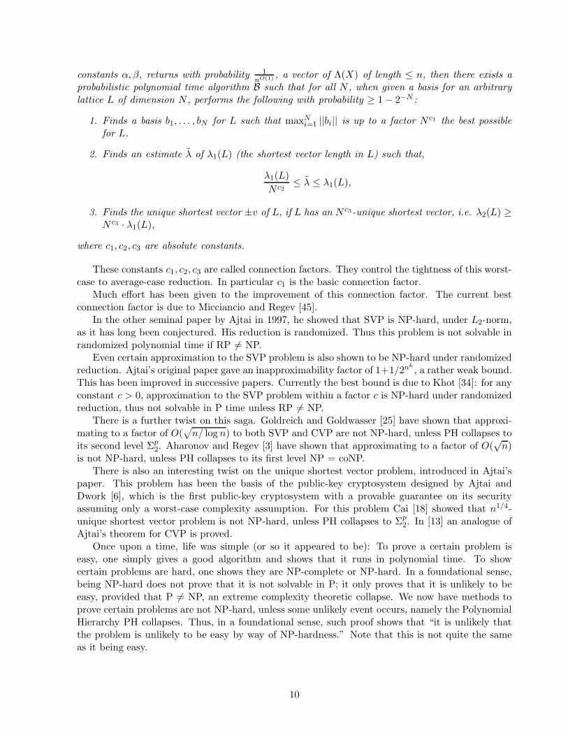
constants α, β, returns with probability 1nO(1) , a vector of Λ(X) of length ≤ n, then there exists a

probabilistic polynomial time algorithm B such that for all N , when given a basis for an arbitrarylattice L of dimension N , performs the following with probability ≥ 1 − 2−N :

1. Finds a basis b1, . . . , bN for L such that maxNi=1 ||bi|| is up to a factor N c1 the best possible

for L.

2. Finds an estimate λ of λ1(L) (the shortest vector length in L) such that,

λ1(L)

N c2≤ λ ≤ λ1(L),

3. Finds the unique shortest vector ±v of L, if L has an N c3-unique shortest vector, i.e. λ2(L) ≥N c3 · λ1(L),

where c1, c2, c3 are absolute constants.

These constants c1, c2, c3 are called connection factors. They control the tightness of this worst-case to average-case reduction. In particular c1 is the basic connection factor.

Much effort has been given to the improvement of this connection factor. The current bestconnection factor is due to Micciancio and Regev [45].

In the other seminal paper by Ajtai in 1997, he showed that SVP is NP-hard, under L2-norm,as it has long been conjectured. His reduction is randomized. Thus this problem is not solvable inrandomized polynomial time if RP 6= NP.

Even certain approximation to the SVP problem is also shown to be NP-hard under randomizedreduction. Ajtai’s original paper gave an inapproximability factor of 1+1/2nk

, a rather weak bound.This has been improved in successive papers. Currently the best bound is due to Khot [34]: for anyconstant c > 0, approximation to the SVP problem within a factor c is NP-hard under randomizedreduction, thus not solvable in P time unless RP 6= NP.

There is a further twist on this saga. Goldreich and Goldwasser [25] have shown that approxi-mating to a factor of O(

√

n/ log n) to both SVP and CVP are not NP-hard, unless PH collapses toits second level Σp

2. Aharonov and Regev [3] have shown that approximating to a factor of O(√

n)is not NP-hard, unless PH collapses to its first level NP = coNP.

There is also an interesting twist on the unique shortest vector problem, introduced in Ajtai’spaper. This problem has been the basis of the public-key cryptosystem designed by Ajtai andDwork [6], which is the first public-key cryptosystem with a provable guarantee on its securityassuming only a worst-case complexity assumption. For this problem Cai [18] showed that n1/4-unique shortest vector problem is not NP-hard, unless PH collapses to Σp

2. In [13] an analogue ofAjtai’s theorem for CVP is proved.

Once upon a time, life was simple (or so it appeared to be): To prove a certain problem iseasy, one simply gives a good algorithm and shows that it runs in polynomial time. To showcertain problems are hard, one shows they are NP-complete or NP-hard. In a foundational sense,being NP-hard does not prove that it is not solvable in P; it only proves that it is unlikely to beeasy, provided that P 6= NP, an extreme complexity theoretic collapse. We now have methods toprove certain problems are not NP-hard, unless some unlikely event occurs, namely the PolynomialHierarchy PH collapses. Thus, in a foundational sense, such proof shows that “it is unlikely thatthe problem is unlikely to be easy by way of NP-hardness.” Note that this is not quite the sameas it being easy.

10

6 Pseudorandomness and Extractors

Monte-Carlo algorithms have been used for many years since the time of Nicholas Metropolis andStanislaw Ulam [43]. Closely related is the notion of a pseudorandom generator. In the traditionaltreatment, e.g. in the multi volume treatise by Knuth [37], the study of pseudorandom generatorsas used in algorithms was given substantial coverage, mainly in terms of various statistical tests.Here the set up is as follows. One has some particular process to generate a sequence of numbersor bits, such as a linear congruential generator. Then we can design a certain statistical test, andsay that a sequence of numbers generated by this process passes the statistical test, if it behavessimilarly to the statistical test as a true random sequence. If this is so, the generating processis called a pseudorandom generator. As an example of a simple minded statistical test, one cancount the number of bits 0’s and 1’s, and a pseudorandom sequence should have roughly the samenumber of 0’s and 1’s.

This ad hoc view of pseudorandom generator was revolutionized by the work of Blum and Micali[12] and by Yao [73] in 1982. Assume a complexity theoretic hardness on the problem of DiscreteLogarithm (This is the following problem: given a prime modulus p and a generator g ∈ Z∗p, fory = gx mod p find the index x), Blum and Micali gave a pseudorandom generator which provablyhas the following property to any polynomial time bounded computer: Given any initial segmentof the bits of the sequence, the next bit is essentially unpredictable. It was Yao who gave whathas become the standard definition of pseudorandomness: No polynomial time bounded computerM can tell apart the pseudorandom sequence and true random sequence. More precisely, supposeGn is a generator mapping 0, 1k(n) → 0, 1n, n ∈ N, then for all polynomial p(n) and for allpolynomial time bounded TM M , for all sufficiently large n,

∣

∣

∣Prx∈0,1n [M(x) = 1] − Pry∈0,1k(n) [M(Gn(y)) = 1]∣

∣

∣ <1

p(n).

Yao proved that his general notion of pseudorandomness is equivalent to Blum-Micali’s next-bitunpredictability against all polynomial time bounded TM. He also showed that starting with anyone-way permutation one can construct a polynomial time computable pseudorandom generator.A function is called a one-way function if it is easy to compute but difficult to invert, all formallydefined in terms of polynomial time computability. The Discrete Logarithm function used byBlum and Micali is an example of a (presumed) one-way permutation. This idea of passing allpolynomial time statistical tests, and its equivalence to the next-bit unpredictability test, has beenthe foundation of all the development that follows.

After a great deal of successive improvements by many researchers, finally Hastad, Impagliazzo,Levin and Luby [29] succeeded in proving the following definitive theorem: Starting with anyone-way function, one can construct a pseudorandom generator.

This proof has two main ideas, besides many technical details. The first is the idea of Goldreichand Levin of a hardcore bit. They showed that if f is a one-way function mapping 0, 1n to 0, 1n,then a random inner product bit X · Y is unpredictable (the hardcore bit) to any polynomial timeadversary, given a uniformly chosen random Y ∈ 0, 1n, and f(X) ∈ 0, 1n where X is chosenuniformly random (but hidden to the adversary) from 0, 1n. The second main idea in thiselaborate proof is the idea of universal hashing (which is due to Carter and Wegman from 1979[20], an idea originated within Theoretical Computer Science and found many practical applicationsall over computer science.)

Another important theorem that came out of Yao’s ground breaking work on the pseudoran-domness is his famous XOR lemma. This essentially says that if f : 0, 1n → 0, 1 and f(X) is

11

slightly unpredictable to a polynomial time adversary, for uniformly chosen X ∈ 0, 1n, then theExclusive-Or bit f(X1) ⊕ f(X2) ⊕ . . . ⊕ f(Xm) is exponentially (in m) more unpredictable.

We now go on to discuss extractor constructions. This is a topic that has seen some of the mostbrilliant ideas and technical depth, and is still very active. We will only be able to describe a smallpart of it.

In the early 1980s, people started to be interested in the question of what happens if therandom source given to a randomized algorithm is not really random, but correlated in some way.For example, maybe the sequence is generated by a linear congruential generator. (In most softwaresystems whenever you call a RANDOM number in a program, this linear congruential generatoror some versions of it is most likely what you get.) Or maybe the sequence is generated by anunderlying random process, such as a Markov chain, which has a bias depending on the underlying(hidden) state. Or maybe the sequence is generated by a physical process which has a certainguarantee (based on quantum mechanics?) that every next bit Xi generated has a certain amountof randomness, such as Pr[Xi = 1] ∈ [ǫ, 1 − ǫ], but nevertheless is dependent on the previous bits(or even controlled by an adversary).

There are results in both the positive and negative directions. As an example of an earlyresult in the positive direction, Santha and U. Vazirani [58], and U. Vazirani and V. Vazirani[72] showed how to construct guaranteed pseudorandom sequences from “slightly-random” sources.(We omit their formal definitions here as they are generally subsumed by the subsequent extractormachineries.) On the negative side, it was shown that linear congruential generators are insufficientfor Quicksort.

It was Nisan and Zuckerman in 1996 [51] who first realized the unifying concept and defined thenotion of an Extractor. We first define min-entropy: Given a distribution X on 0, 1n, the min-entropy, H∞(X), is defined as H∞(X) = minx(− log2(Pr[X = x])). Thus, 2−H∞(X) is the largestprobability assigned to any point. Intuitively H∞(X) represents the number of true random bitscontained in X.

An extractor extracts the randomness contained in a random source X, with the help of someadditional true random bits.

Definition 6.1 An (n, d, k,m, ǫ)-extractor is a function Ext : 0, 1n × 0, 1d → 0, 1m, suchthat whenever a distribution X on 0, 1n has H∞(X) ≥ k,

||Ext(X,Ud) − Um|| ≤ ǫ.

Here Uℓ is the uniform distribution on 0, 1ℓ, and || · || denotes statistical distance. The statis-tical distance between two distributions X and Y on the same set is defined to be ||X − Y || =maxD |PrX [D]−PrY [D]|. Ideally, we would like to maximize m to be close to k, while minimize dand ǫ.

It can be shown that without using additional random bits Ud, this is impossible. Non-constructively it can be shown that for every n, k ≤ n and ǫ > 0, there exists a (n, d, k,m, ǫ)-extractor with m = k and d = O(log(n/ǫ)). However the challenging task is to construct explicitextractors, computable in polynomial time.

Explicit constructions of extractors have many applications. Among them: simulation of ran-domized algorithms, constructions of oblivious samplers, randomness-efficient error reductions, ex-plicit constructions of expanders, sorting networks, hardness of approximation, and pseudorandomgenerators for space-bounded computations.

In 2003, Lu, Reingold, Vadhan, and Wigderson [41] gave a construction that is optimal up tosome constant factors: for every constants α > 0, ǫ > 0, they gave a (n, d, k,m, ǫ)-extractor, for all

12

n, k ≤ n and, m = (1 − α)k and d = O(log n). That is, their extractor can extract m = (1 − α)kbits of entropy from any source with H∞(X) ≥ k, using only O(log n) bits of additional randombits.

However, their construction uses many previous constructions and techniques, and these tech-niques have undergone many rounds of improvements, that it is infeasible to give a coherent ac-count in a few pages. Instead we will give an account of an elegant construction by Trevisan [65],as improved by Raz, Reingold and Vadhan [54]. This construction introduced techniques that areimportant in many aspects, and it is representative of the more recent research in ComputationalComplexity Theory, such as the use of finite fields, the connection to coding theory, and the use ofcombinatorial designs.

There are two main ingredients of this construction. The first is the use of error correctingcode. The second is a combinatorial design, first used by Nisan and Wigderson.

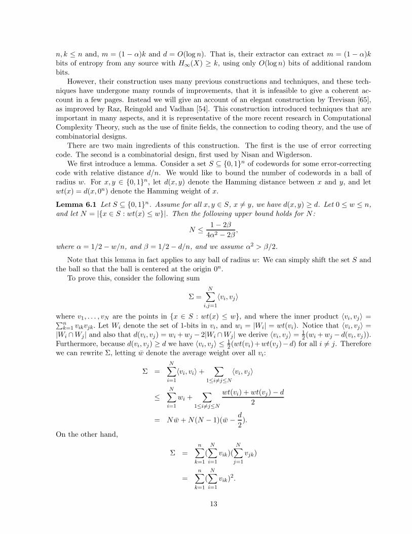
We first introduce a lemma. Consider a set S ⊆ 0, 1n of codewords for some error-correctingcode with relative distance d/n. We would like to bound the number of codewords in a ball ofradius w. For x, y ∈ 0, 1n, let d(x, y) denote the Hamming distance between x and y, and letwt(x) = d(x, 0n) denote the Hamming weight of x.

Lemma 6.1 Let S ⊆ 0, 1n. Assume for all x, y ∈ S, x 6= y, we have d(x, y) ≥ d. Let 0 ≤ w ≤ n,and let N = |x ∈ S : wt(x) ≤ w|. Then the following upper bound holds for N :

N ≤ 1 − 2β

4α2 − 2β,

where α = 1/2 − w/n, and β = 1/2 − d/n, and we assume α2 > β/2.

Note that this lemma in fact applies to any ball of radius w: We can simply shift the set S andthe ball so that the ball is centered at the origin 0n.

To prove this, consider the following sum

Σ =N

∑

i,j=1

〈vi, vj〉

where v1, . . . , vN are the points in x ∈ S : wt(x) ≤ w, and where the inner product 〈vi, vj〉 =∑n

k=1 vikvjk. Let Wi denote the set of 1-bits in vi, and wi = |Wi| = wt(vi). Notice that 〈vi, vj〉 =|Wi ∩Wj | and also that d(vi, vj) = wi + wj − 2|Wi ∩Wj| we derive 〈vi, vj〉 = 1

2 (wi + wj − d(vi, vj)).Furthermore, because d(vi, vj) ≥ d we have 〈vi, vj〉 ≤ 1

2(wt(vi)+wt(vj)−d) for all i 6= j. Thereforewe can rewrite Σ, letting w denote the average weight over all vi:

Σ =N

∑

i=1

〈vi, vi〉 +∑

1≤i6=j≤N

〈vi, vj〉

≤N

∑

i=1

wi +∑

1≤i6=j≤N

wt(vi) + wt(vj) − d

2

= Nw + N(N − 1)(w − d

2).

On the other hand,

Σ =n

∑

k=1

(N

∑

i=1

vik)(N

∑

j=1

vjk)

=n

∑

k=1

(N

∑

i=1

vik)2.

13

Let Xk =∑N

i=1 vik be the number of vi that have a 1 in the kth position. Then∑

k Xk is the totalnumber of 1’s over all vi, and therefore

∑

k Xk = Nw. By convexity, we obtain the lower bound:

Σ =n

∑

k=1

X2k ≥ n

(∑

k Xk

n

)2

=(Nw)2

n.

Combining these two bounds, we get

N ≤d2n

( wn )2 − ( w

n ) + d2n

=1 − 2β

4α′2 − 2β,

where β = 12 − d

n and α′ = 12 − w

n . As each wi ≤ w, we have w ≤ w, and so for α = 12 − w

n we haveα′ ≥ α, and it follows that

N ≤ 1 − 2β

4α2 − 2β.

Setting α =√

γ and β = γ/2. We get:

Corollary 6.1 If every pair of points in S ⊆ 0, 1n has relative distance at least 1−γ2 , then every

ball of relative radius at most 1/2 −√γ contains at most 1/3γ < 1/γ points in S.

We briefly review the Reed-Soloman Code. Let F = GF [2m], and let α0, α1, . . . , αk−1 ∈ F. TheReed-Solomon (RS) encoding of α = α0 . . . αk−1 interprets the αi as coefficients of a polynomial ofdegree k − 1; that is, α defines the polynomial

fα(x) = α0 + α1x + α2x2 + . . . + αk−1x

k−1.

Then the RS encoding of α, RS(α), is the concatenation of function values of fα evaluated at allpoints ai in the field F:

RS : α 7→ (fα(a1), fα(a2), . . . , fα(a|F|)).

Equivalently, we may consider the 2m × k matrix

M =

1 a1 a21 a3

1 . . . ak−11

1 a2 a22 a3

2 . . . ak−12

1 a3 a23 a3

3 . . . ak−13

......

......

. . ....

and let α = (α0, . . . , αk−1)T , so that the RS encoding of α is Mα. Note that if α 6= β then the

corresponding polynomials fα 6= fβ can agree on at most k − 1 points. It follows that the RSencodings RS(α) and RS(β) must disagree on at least |F| − (k − 1) = 2m − (k − 1) entries.

Our goal is to design a binary code of polynomial length (and polynomial time computable)with the property that the relative distance of code words is almost 1/2. Even though the RS codehas the property that two distinct words differ on most entries, measured as a binary code, twodifferent values in F may still have many identical bit positions. One easy method to get aroundthis is via a process called code concatenation.

Thus we introduce the Hadamard code (Had). This code has 2m code words each of length 2m.Consider a 2m × 2m matrix Hm with 0, 1 entries. Each row and column of Hm = (hx,y) is indexedby x, y ∈ Zm

2 , and has the value hx,y = 〈x, y〉 mod 2, the inner product mod 2. Each m bit stringx ∈ Zm

2 is coded as a 2m long code word Had(x) = (hx,y)y∈Zm2

. Note that whenever x 6= x′, Had(x)and Had(x′) differ by exactly half of 2m entries.

14

Now we can consider the concatenation of the Reed-Soloman code with the Hadamard code.Given α ∈ 0, 1n, the Reed-Solomon code treats α as specifying the coefficients of a degreed

.= ⌈n/m⌉ − 1 polynomial over a field F where |F| = 2m. For α 6= α′, the code words RS(α) and

RS(α′) differ on at least 2m − d entries. By taking

ECn,m(α) = (Had(pα(a1)),Had(pα(a2)), . . . ,Had(pα(a|F|))),

we get a binary code of length 22m and relative distance at least (2m−d)2m/222m ≥ 1

2 − n2m+1 . For any

δ > 0, we let m = ⌈log(n/δ2)⌉, then n = 22m = O(n2/δ4) is the length of the code, and the relative

distance ≥ 12 − δ2

2 . We will denote this code ECn,m as ECn,δ(α) from now. Therefore, by theCorollary, any ball of relative radius 1

2 − δ contains at most 1δ2 points from the code.

Lemma 6.2 For all n ∈ N and δ > 0, there exists an error-correcting code ECn,δ : 0, 1n →0, 1n, where n = poly(n, 1

δ ), such that every Hamming ball of relative radius 12 − δ in 0, 1n

contains at most 1δ2 codewords. Furthermore, ECn,δ can be computed in time poly(n, 1

δ ), and n isa power of 2.

A second ingredient of this extractor construction is the idea of a combinatorial design. Tre-visan’s construction directly uses a design first used by Nisan and Widgerson. The RRV construc-tion (by Raz, Reingold and Vadhan) uses a slightly improved version called a weak design. Wewant a set system of large cardinality but with pairwise small intersections. The Nisan-Widgersondesign requires that this intersection being small for all pairs, the RRV weak design only requiresthis in an aggregate sense.

More formally,

Definition 6.2 For ℓ ∈ N, ρ ≥ 1, an (ℓ, ρ)-design is a collection S = S1, . . . , Sm with Si ⊂ [d]such that:

• ∀i, |Si| = ℓ, and

• ∀i 6= j, |Si ∩ Sj | ≤ log ρ.

The Nisan-Widgerson design uses low degree polynomials as follows. Let q be a prime power,d = q2, then each set Si is determined by a polynomial f of some degree bound D, such thatSi = (a, f(a)) | a ∈ Fq. Then each |Si| = q and Si ⊂ [d]. Since distinct polynomials of degree atmost D can agree at most D points, |Si ∩ Sj| ≤ D, for i 6= j. The astute reader will recognize thatthis is a generalization of the projective plane (here actually an affine plane) over a finite field. (Inthe projective plane, we use linear polynomials. Here the polynomials f are of degree bounded bysome upper bound D.)

A weak design is defined as follows:

Definition 6.3 For ℓ ∈ N, ρ ≥ 1, a weak (ℓ, ρ)-design is a collection S = S1, . . . , Sm withSi ⊂ [d] such that:

• ∀i, |Si| = ℓ, and

• ∀i,∑

j<i 2|Si∩Sj | ≤ ρ(m − 1).

Note that if S is a (ℓ, ρ)-design, then it is also a weak (ℓ, ρ)-design.We are now ready to describe the Trevisan and RRV extractor. Let m ≤ k ≤ n, and ǫ > 0.

It takes an imperfect random source of n bits with min-entropy k as well as d uniform bits, and

15

outputs m bits that are ǫ-close to uniform. Let δ = ǫ/4m, and consider the error correctingcode ECn,δ.

1 Define ℓ = log2 n and let S be a weak (ℓ, ρ)-design. We will first apply ECn,δ to theimperfect random bits to generate n bits. Then these n bits is viewed as a truth table for a Booleanfunction u on ℓ bits. We will then apply the function u to different subsets of the d random bits,choosing which subsets using the design S, and this will be the output of the generator. (This lastpart of the extractor—choosing different subsets using a design, and then evaluating a function atthese subsets of bits—is just the Nisan-Wigderson generator using u as the hard function with seedy ∈U 0, 1d.)

ExtS : 0, 1n × 0, 1d → 0, 1m

ExtS(u, y) = NWS,u(y) = u(y|S1) · · · u(y|Sm)

where u = ECn,δ(u).We now outline a proof that ExtS is an extractor. In fact it is a strong extractor, i.e., even

with the additional d random bits present, (Ud,ExtS(X,Ud)) is ǫ-close to the uniform distributionUm+d for any X with H∞(X) ≥ k.

We prove by contradiction. Suppose this is not true, then for some distribution X on 0, 1n

with H∞(X) ≥ k, the output of (Ud,ExtS) can be distinguished from the uniform distribution by> ǫ. Then by a classical argument due to Yao, using an interpolation of distributions, one can showfor some i, there exists a next-bit predictor A : 0, 1d × 0, 1i−1 → 0, 1,

Pry∈U0,1d,u←X

[A(y, u(y|S1), . . . , u(y|Si−1)) = u(y|Si)] >1

2+

ǫ

m.

In other words, when given y ∈U 0, 1d and u(y|S1), . . . , u(y|Si−1), A will provide the correct valueof u(y|Si) with probability > 1/2 + ǫ/m.

Consider the set B of “bad” u, for which A provides a good prediction to u(y|Si),

Pry∈U0,1d

[A(y, u(y|S1), . . . , u(y|Si−1)) = u(y|Si)] >1

2+

ǫ

2m.

For any u, letp = Pr

y[A(y, u(y|S1), . . . , u(y|Si−1)) = u(y|Si)].

If we focus on the ℓ = |Si| bits within Si, by an averaging argument, we can set all the other bits0, 1d − Si to some particular 0-1 assignment, and preserve this probability p.

Prx

[A(y(x), u(y(x)|S1), . . . , u(y(x)|Si−1)) = u(x)] ≥ p,

where x = y|Si , and y(x) is y with all the bits in 0, 1d − Si already set to some 0-1 constants.Now, each function u(y(x)|Sj ), for j < i, is a Boolean function on Si ∩ Sj , which can be speci-

fied by a truth table of length 2|Si∩Sj |, Therefore the set of sequences of Boolean functions x 7→(y(x), u(y(x)|S1), . . . , u(y(x)|Si−1)) can be counted by a binary string of length

∑

j<i 2|Si∩Sj | ≤

ρ(m − 1). Let F denote the set of all such sequences of Boolean functions. Then |F| < 2ρm. Thisis a consequence of the weak-design S.

Then, each u ∈ B satisfies the following property: There exists some f ∈ F , such that

Prx

[A(f(x)) = u(x)] = Prx

[A(y(x), u(y(x)|S1), . . . , u(y(x)|Si−1)) = u(x)] ≥ p >1

2+

ǫ

2m.

1The output size of the extractor is customarily denoted as m, and is unrelated to the field size chosen for ECn,δ ,which is ≈ n/δ2.

16

But we can view the Boolean function A(f(·)) as a binary string, via its truth table, of lengthn, and then the probability Prx[A(f(x)) 6= u(x)] has another interpretation, namely the relativeHamming distance between these two strings in 0, 1n. Thus Prx[A(f(x)) = u(x)] > 1

2 + ǫ2m is the

same as relative Hamming distance < 12 − ǫ

2m .Now recall our u is the output of our error correcting code ECn,δ, it follows that within the

relative Hamming distance 12 − ǫ

2m of A(f(·)) there can be at most (2m/ǫ)2 strings u. This is aconsequence of the error correcting code ECn,δ.

Thus|B| ≤ (2m/ǫ)2|F| < (2m/ǫ)22ρm.

It is possible to have a weak-design S with ρ = (k−3 log2(m/ǫ)−3)/m. Since X has min-entropyk, it follows that

Pru←X

[u ∈ B] < (2m/ǫ)22ρm · 2−k = ǫ/2m.

On the other hand, if u 6∈ B, then by definition

Pry∈U0,1d

[A(y, u(y|S1), . . . , u(y|Si−1)) = u(y|Si)] ≤1

2+

ǫ

2m.

Combining,

Pry∈U0,1d,u←X

[A(y, u(y|S1), . . . , u(y|Si−1)) = u(y|Si)] ≤ Pru←X

[u ∈ B] + Pru←X

[u 6∈ B]

(

1

2+

ǫ

2m

)

≤ ǫ

2m+

(

1

2+

ǫ

2m

)

=1

2+

ǫ

m,

This contradicts the performance of the predictor A.

Theorem 6.1 ∀n, k,m ∈ N, ǫ > 0,m ≤ k ≤ n, there exists an explicit (n, d, k,m, ǫ)-extractor with

d = O

(

log2(nǫ)

log( km

)

)

.

7 Valiant’s New Theory of Holographic Algorithms

In a remarkable paper, Valiant [69] in 2004 has proposed a completely new theory of HolographicAlgorithms or Holographic Reductions. The theory is quite unlike anything before that it is prob-ably fair to say that at this point few people in the world understands or appreciates its full reachand potentials. (We are certainly not among those.)

It is a delicate theory that will be difficult to explain without all the definitions. At the heart ofthe new theory, one can say that Valiant has succeeded in devising a custom made process which iscapable of carrying out a seemingly exponential computation with exponentially many cancellationsso that the computation can actually be done in polynomial time. One can view this new theoryas another algorithmic design paradigm, much like greedy algorithms, or divide-and-conquer, ordynamic programming etc, which pushes back the frontier of what is solvable by polynomial time.Admittedly, at this early stage, it is still premature to say what drastic consequence it might haveon the landscape of the big questions of complexity theory, such as P vs. NP. But the new theoryhas already been used by Valiant to devise polynomial time algorithms for a number of problems.All these problems appear to be very close to NP-complete or NP-hard problems in one way or

17

another. All of which were thought to have no known polynomial time algorithms, and all appearto need the new machinery to show their membership in P. 2

Unless and until a proof of P 6= NP is found, one should regard this conjecture as just that, anunproven conjecture. We can ask ourselves on what basis we derive confidence on the truth of thisconjecture. In our view, frankly, it is not for any partial lower bound. While generally ingeniousand difficult to prove, all lower bounds we currently have are either for very restricted models ofcomputation or are still very weak. Fundamentally this source of confidence in P 6= NP comes fromthe fact that all existing algorithmic approaches do not seem to tackle these NP-complete problems.Well, when there is a new algorithmic design paradigm being found, one must re-examine all thesebeliefs critically.

We now give a brief description of this theory. Playing what seems to be a fundamental role isthe planar matching problem. Given a graph G, a matching of G is a set of edges no two of whichshare a vertex. A perfect matching M is a matching such that every vertex of G is incident to oneedge of M . The decision problem of whether there is a perfect matching in G is computable in P,one of the notable achievements in the study of Algorithms. However, it is known that countingthe number of perfect matchings in G is #P-complete.

We assign to every edge e = (i, j) a variable xij, where i < j. Then we define the followingpolynomial

PerfMatch(G) =∑

M

∏

(i,j)∈M

xij ,

where the sum is over all perfect matchings M . PerfMatch(G) is a polynomial on(n2

)

many variablesxij, where 1 ≤ i < j ≤ n. If the graph is a weighted graph with weights wij, we can also evaluatePerfMatch(G) at xij = wij. Note that if all the weights are 1, then PerfMatch(G) just counts thenumber of perfect matchings in the graph.

A most remarkable result due to Fisher, Kasteleyn and Temperly (FKT), ([64], [35], and [36])from statistical physics is that for planar graphs, this Perfect Matching polynomial PerfMatch(G)can be evaluated in polynomial time. In fact it can be evaluated as a Pfaffian of a skew-symmetricmatrix which is constructible from a planar embedding of G in polynomial time, (and a planarembedding of G can also be computed from a planar graph G given by its adjacency matrix inpolynomial time).

In effect, all of Valiant’s successes on these problems for which he found P time algorithms for thefirst time are obtained by a certain reduction to this planar Perfect Matching polynomial evaluation.These reductions are called holographic reductions, because they carry out exponentially manycancellations in a pattern of interference that is “tailor made” for the problem.

Consider a graph which is a line segment with 4 vertices 1, 2, 3, 4 and 3 edges (1, 2), (2, 3), (3, 4)with weights −1, 1 and 1 respectively. The PerfMatch(G) is −1, as (1, 2), (3, 4) is the uniqueperfect matching. If we remove either the left or the right end vertex then there are no more perfectmatchings and therefore PerfMatch(G − 1) = PerfMatch(G − 4) = 0. If we remove both endvertices then we have a unique perfect matching again (2, 3) and PerfMatch(G − 1, 4) = 1.

Generally we define a planar matchgate Γ as a triple (G,X, Y ) where G is a planar embeddingof a weighted planar graph (V,E,W ), where X ⊆ V is a set of input nodes, Y ⊆ V is a set ofoutput nodes, and X ∩ Y = ∅. Furthermore in the planar embedding of G, counter-clock wise oneencounters vertices of X, labeled 1, . . . , |X| and then vertices of Y , labeled |Y |, . . . , 1. Now the

2In a most recent version of [69], available in ECCC, Valiant has found that for a few problems on that list, thereis an alternative approach using classical reductions from a problem called #PL-CUT. This works with respect to aparticular basis called b2. But even for this basis, macthgates of arity 4 still appear to be out of reach by classicalreductions.

18

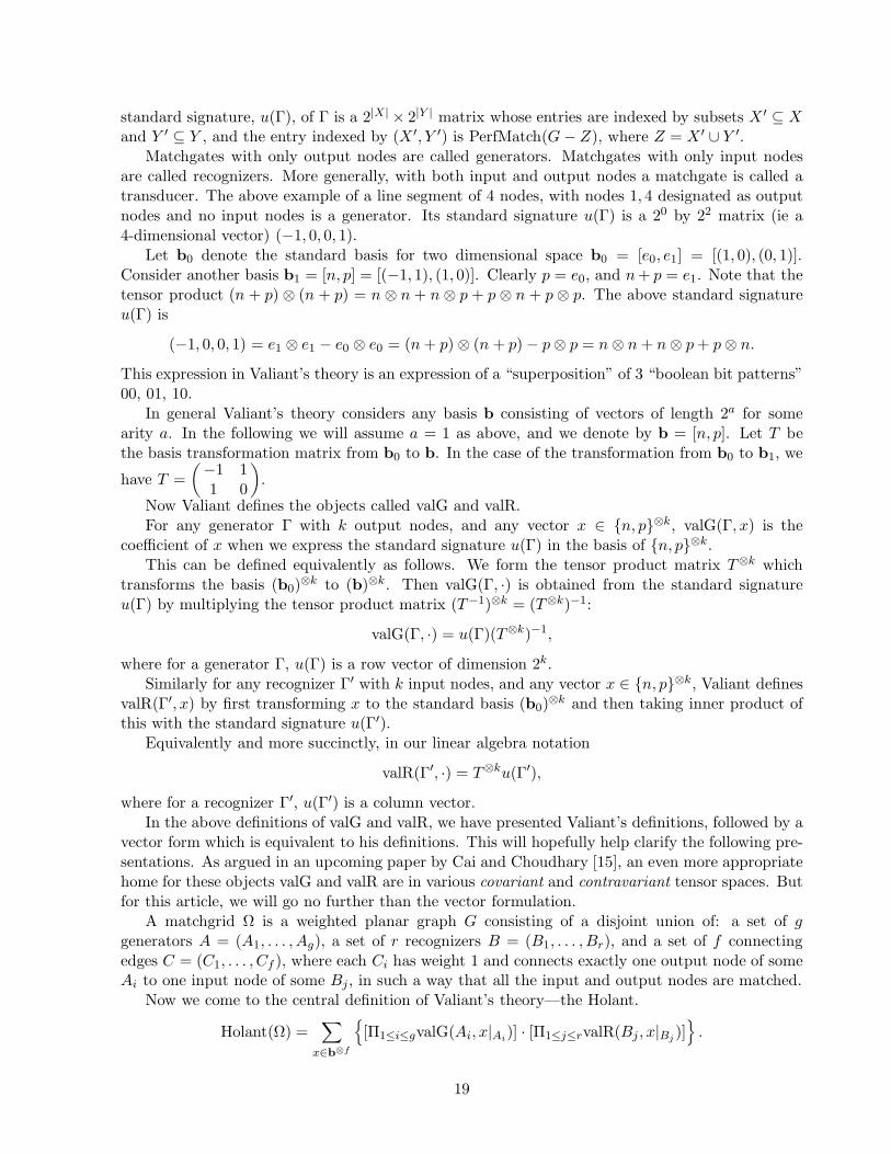
standard signature, u(Γ), of Γ is a 2|X| × 2|Y | matrix whose entries are indexed by subsets X ′ ⊆ Xand Y ′ ⊆ Y , and the entry indexed by (X ′, Y ′) is PerfMatch(G − Z), where Z = X ′ ∪ Y ′.

Matchgates with only output nodes are called generators. Matchgates with only input nodesare called recognizers. More generally, with both input and output nodes a matchgate is called atransducer. The above example of a line segment of 4 nodes, with nodes 1, 4 designated as outputnodes and no input nodes is a generator. Its standard signature u(Γ) is a 20 by 22 matrix (ie a4-dimensional vector) (−1, 0, 0, 1).

Let b0 denote the standard basis for two dimensional space b0 = [e0, e1] = [(1, 0), (0, 1)].Consider another basis b1 = [n, p] = [(−1, 1), (1, 0)]. Clearly p = e0, and n + p = e1. Note that thetensor product (n + p) ⊗ (n + p) = n ⊗ n + n ⊗ p + p ⊗ n + p ⊗ p. The above standard signatureu(Γ) is

(−1, 0, 0, 1) = e1 ⊗ e1 − e0 ⊗ e0 = (n + p) ⊗ (n + p) − p ⊗ p = n ⊗ n + n ⊗ p + p ⊗ n.

This expression in Valiant’s theory is an expression of a “superposition” of 3 “boolean bit patterns”00, 01, 10.

In general Valiant’s theory considers any basis b consisting of vectors of length 2a for somearity a. In the following we will assume a = 1 as above, and we denote by b = [n, p]. Let T bethe basis transformation matrix from b0 to b. In the case of the transformation from b0 to b1, we

have T =

(−1 11 0

)

.

Now Valiant defines the objects called valG and valR.For any generator Γ with k output nodes, and any vector x ∈ n, p⊗k, valG(Γ, x) is the

coefficient of x when we express the standard signature u(Γ) in the basis of n, p⊗k.This can be defined equivalently as follows. We form the tensor product matrix T⊗k which

transforms the basis (b0)⊗k to (b)⊗k. Then valG(Γ, ·) is obtained from the standard signature

u(Γ) by multiplying the tensor product matrix (T−1)⊗k = (T⊗k)−1:

valG(Γ, ·) = u(Γ)(T⊗k)−1,

where for a generator Γ, u(Γ) is a row vector of dimension 2k.Similarly for any recognizer Γ′ with k input nodes, and any vector x ∈ n, p⊗k, Valiant defines

valR(Γ′, x) by first transforming x to the standard basis (b0)⊗k and then taking inner product of

this with the standard signature u(Γ′).Equivalently and more succinctly, in our linear algebra notation

valR(Γ′, ·) = T⊗ku(Γ′),

where for a recognizer Γ′, u(Γ′) is a column vector.In the above definitions of valG and valR, we have presented Valiant’s definitions, followed by a

vector form which is equivalent to his definitions. This will hopefully help clarify the following pre-sentations. As argued in an upcoming paper by Cai and Choudhary [15], an even more appropriatehome for these objects valG and valR are in various covariant and contravariant tensor spaces. Butfor this article, we will go no further than the vector formulation.

A matchgrid Ω is a weighted planar graph G consisting of a disjoint union of: a set of ggenerators A = (A1, . . . , Ag), a set of r recognizers B = (B1, . . . , Br), and a set of f connectingedges C = (C1, . . . , Cf ), where each Ci has weight 1 and connects exactly one output node of someAi to one input node of some Bj, in such a way that all the input and output nodes are matched.

Now we come to the central definition of Valiant’s theory—the Holant.

Holant(Ω) =∑

x∈b⊗f

[Π1≤i≤gvalG(Ai, x|Ai)] · [Π1≤j≤rvalR(Bj , x|Bj )]

.

19

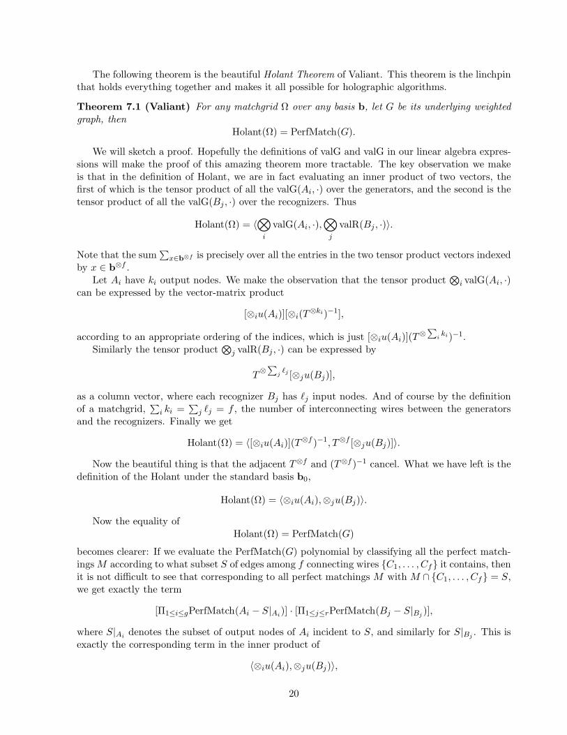
The following theorem is the beautiful Holant Theorem of Valiant. This theorem is the linchpinthat holds everything together and makes it all possible for holographic algorithms.

Theorem 7.1 (Valiant) For any matchgrid Ω over any basis b, let G be its underlying weightedgraph, then

Holant(Ω) = PerfMatch(G).

We will sketch a proof. Hopefully the definitions of valG and valG in our linear algebra expres-sions will make the proof of this amazing theorem more tractable. The key observation we makeis that in the definition of Holant, we are in fact evaluating an inner product of two vectors, thefirst of which is the tensor product of all the valG(Ai, ·) over the generators, and the second is thetensor product of all the valG(Bj , ·) over the recognizers. Thus

Holant(Ω) = 〈⊗

i

valG(Ai, ·),⊗

j

valR(Bj , ·)〉.

Note that the sum∑

x∈b⊗f is precisely over all the entries in the two tensor product vectors indexedby x ∈ b⊗f .

Let Ai have ki output nodes. We make the observation that the tensor product⊗

i valG(Ai, ·)can be expressed by the vector-matrix product

[⊗iu(Ai)][⊗i(T⊗ki)−1],

according to an appropriate ordering of the indices, which is just [⊗iu(Ai)](T⊗

∑

iki)−1.

Similarly the tensor product⊗

j valR(Bj , ·) can be expressed by

T⊗

∑

jℓj [⊗ju(Bj)],

as a column vector, where each recognizer Bj has ℓj input nodes. And of course by the definitionof a matchgrid,

∑

i ki =∑

j ℓj = f , the number of interconnecting wires between the generatorsand the recognizers. Finally we get

Holant(Ω) = 〈[⊗iu(Ai)](T⊗f )−1, T⊗f [⊗ju(Bj)]〉.

Now the beautiful thing is that the adjacent T⊗f and (T⊗f )−1 cancel. What we have left is thedefinition of the Holant under the standard basis b0,

Holant(Ω) = 〈⊗iu(Ai),⊗ju(Bj)〉.

Now the equality ofHolant(Ω) = PerfMatch(G)

becomes clearer: If we evaluate the PerfMatch(G) polynomial by classifying all the perfect match-ings M according to what subset S of edges among f connecting wires C1, . . . , Cf it contains, thenit is not difficult to see that corresponding to all perfect matchings M with M ∩ C1, . . . , Cf = S,we get exactly the term

[Π1≤i≤gPerfMatch(Ai − S|Ai)] · [Π1≤j≤rPerfMatch(Bj − S|Bj )],

where S|Ai denotes the subset of output nodes of Ai incident to S, and similarly for S|Bj . This isexactly the corresponding term in the inner product of

〈⊗iu(Ai),⊗ju(Bj)〉,

20

proving the Theorem.

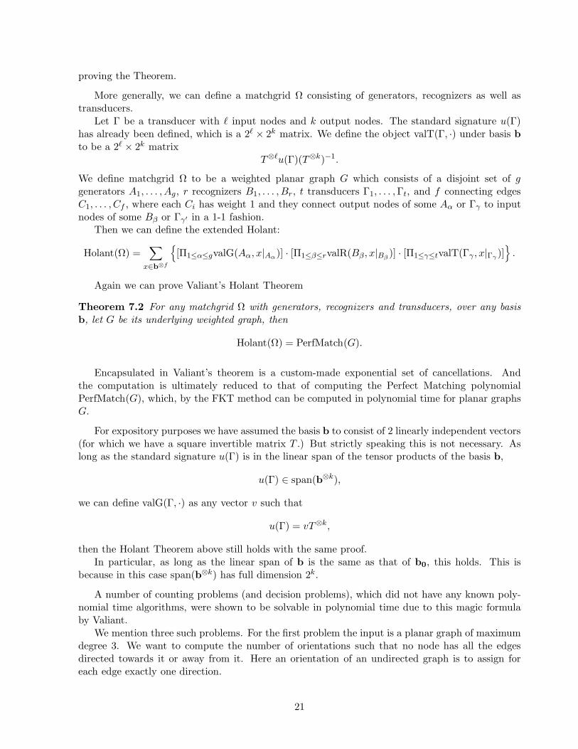
More generally, we can define a matchgrid Ω consisting of generators, recognizers as well astransducers.

Let Γ be a transducer with ℓ input nodes and k output nodes. The standard signature u(Γ)has already been defined, which is a 2ℓ × 2k matrix. We define the object valT(Γ, ·) under basis bto be a 2ℓ × 2k matrix

T⊗ℓu(Γ)(T⊗k)−1.

We define matchgrid Ω to be a weighted planar graph G which consists of a disjoint set of ggenerators A1, . . . , Ag, r recognizers B1, . . . , Br, t transducers Γ1, . . . ,Γt, and f connecting edgesC1, . . . , Cf , where each Ci has weight 1 and they connect output nodes of some Aα or Γγ to inputnodes of some Bβ or Γγ′ in a 1-1 fashion.

Then we can define the extended Holant:

Holant(Ω) =∑

x∈b⊗f

[Π1≤α≤gvalG(Aα, x|Aα)] · [Π1≤β≤rvalR(Bβ, x|Bβ)] · [Π1≤γ≤tvalT(Γγ , x|Γγ )]

.

Again we can prove Valiant’s Holant Theorem

Theorem 7.2 For any matchgrid Ω with generators, recognizers and transducers, over any basisb, let G be its underlying weighted graph, then

Holant(Ω) = PerfMatch(G).

Encapsulated in Valiant’s theorem is a custom-made exponential set of cancellations. Andthe computation is ultimately reduced to that of computing the Perfect Matching polynomialPerfMatch(G), which, by the FKT method can be computed in polynomial time for planar graphsG.

For expository purposes we have assumed the basis b to consist of 2 linearly independent vectors(for which we have a square invertible matrix T .) But strictly speaking this is not necessary. Aslong as the standard signature u(Γ) is in the linear span of the tensor products of the basis b,

u(Γ) ∈ span(b⊗k),

we can define valG(Γ, ·) as any vector v such that

u(Γ) = vT⊗k,

then the Holant Theorem above still holds with the same proof.In particular, as long as the linear span of b is the same as that of b0, this holds. This is

because in this case span(b⊗k) has full dimension 2k.

A number of counting problems (and decision problems), which did not have any known poly-nomial time algorithms, were shown to be solvable in polynomial time due to this magic formulaby Valiant.

We mention three such problems. For the first problem the input is a planar graph of maximumdegree 3. We want to compute the number of orientations such that no node has all the edgesdirected towards it or away from it. Here an orientation of an undirected graph is to assign foreach edge exactly one direction.

21

For the second problem the input is a planar graph of maximum degree 3. We want to computethe cardinality of a smallest subset of vertices such that its removal renders the graph bipartite.This problem is NP-complete for maximum degree 6.

The third problem is called #X-Matchings. After its description we will describe its solutionusing the Holant Theorem. The solutions to the other two problems as well as several others canbe found in [69].

The input to #X-Matchings is a planar weighted bipartite graph G = (V,E,W ) where V ispartitioned into V1 and V2, and every node in V1 has degree 2. The output is the sum of the massesof all matchings of all sizes where the mass of a matching is the product of (1) the weights of allthe edges present in the matching, and (2) the quantity −(w1 + . . . + wk) for all nodes in V2 whichare unmatched, where w1, . . . , wk are all the weights of edges incident to that unmatched node.

Now we will define a matchgrid.For this purpose we will consider the basis b1 = [n, p], and the following gadgets for generators

Ai and recognizers Bj. Each vertex ui of V1 is replaced by a generator Ai, and each Ai is the samegadget. This gadget is the line graph with 4 vertices described as an example earlier illustratingthe Perfect Matching polynomial PerfMatch(G). Its standard signature u(Ai) = (−1, 0, 0, 1) =n⊗ n + n⊗ p + p⊗ n. One can say that this generator generates the “bit pattern” (nn, np, pn, pp)with coefficients (1, 1, 1, 0) under the basis b1. If we think of this corresponds to a “logical bitpattern”, with n for no and p for yes, then this corresponds to allowing having zero or one (eitherone) but not both edges at ui being picked. Such a scenario naturally corresponds to a (notnecessarily perfect) matching at the vertex ui ∈ V1.

The recognizer gadget for each vertex v in V2 of degree d is a “star graph” B with one vertex v0

at the center and d many vertices outside, each connected to v0 by an edge: The vertex set of B isv0, v1, . . . , vd, and edge set is (v0, v1), . . . , (v0, vd), where each edge (v0, vi) inherits the weightin the input graph for the ith edge at v. If the ith edge at v is connected to u ∈ V1, then vi isconnected to an output node of the gadget A for u, and with weight 1. These 2|V1| =

∑

v∈V2deg(v)

edges are the f connecting edges described in the general matchgrid construction.It is clear that this local replacement procedure starting from the planar graph G produces still

a planar graph, which is our matchgrid.For the “star graph” B as a recognizer with d outside vertices as its input nodes, the standard

signature u(B) has dimension 2d. Every subset Z ⊆ 1, . . . , d produces no perfect matchings inB − Z, except those Z which has cardinality exactly d − 1, and in which case the entry in u(B) iswi.

Now consider valR(B, ·). It is not difficult to show that valR(B, ·) is a vector with most entries0, except those entries labelled by x = x1 ⊗ x2 ⊗ . . . ⊗ xd with either all, or all except one, xi = n.If xi = p for one i, and all the rest are n, then the value of valR is wi, where wi is the weight of theith edge at v ∈ V2. If all xi = n, then the value of this entry valR(B,n⊗ n⊗ . . .⊗n) = −∑d

i=1 wi.We can see this as follows: Suppose some x = x1 ⊗ x2 ⊗ . . . ⊗ xd, where xi = n = (−1, 1) or

xi = p = (1, 0), has a non-zero inner product with u(B). We only need to focus on those entriesof u(B) indexed by a subset Z of cardinality exactly d − 1. At an arbitrary entry indexed by Z,the value in the vector x is a product of the second or the first entries of xi, depending on i ∈ Zor not. Thus if |Z| = d − 1, we take the product from the first entry for one xi, and the secondentry from the other xi’s for exactly d − 1 times. If there are more than one xi = p, then for each|Z| = d − 1, for at least one i ∈ Z we have xi = p, and the corresponding factor is the secondentry 0 in p = (1, 0), giving the product value 0. For those x with exactly zero or one xi = p thevalR(B, ·) values are clearly as stated.

Again by a “bit pattern” interpretation with n for no and p for yes, at a vertex v ∈ V2, theonly non-zero valR(B,x) values are those having zero or one xi = p corresponds to (not necessarily

22

perfect) matchings.Now the Holant definition expresses exactly the sum to be computed by the problem #X-

Matchings. On the other hand, the Holant Theorem shows that the Holant can be computed byevaluating the PerfMatch polynomial on the matchgrid via the FKT method in polynomial time.

It was shown by Jerrum [32] that the problem of counting the number of (not necessarilyperfect) matchings in a planar graph is #P-complete. Vadhan [66] showed that this was trueeven for planar bipartite graphs of degree 6. If all vertices have degree 2, the problem is trivial.Therefore the above polynomial time algorithm for #X-Matchings is quite remarkable. Note thatif all vertices in V2 have degree 4 and we set all weights to 1, and evaluate everything modulo 5,then −∑d

i=1 wi = −4 ≡ 1 mod 5. Then we would be evaluating the number of (not necessarilyperfect) matchings in the planar bipartite graph modulo 5, in polynomial time.

Valiant’s Theory of Holographic Algorithms were developed along with a closely related theoryof matchgates in terms of Pfaffians and simulations of certain quantum computations [68, 67, 70, 71].In the Pfaffian based development, one drops the planarity requirement, but adds a complicationof order-overlaps; in this parallel theory, instead of signatures one has the notion of characters. Itappears that there is a great deal of depth and richness to this theory. For instance, these matchgatessatisfy a set of matchgate identities which follow from the Grassmann-Plucker identities. Valiantshowed a set of 5 identities to be satisfied by 2-input 2-output matchgates. Cai, Choudhary andKumar have found a complete set of 10 identities characterizing these matchgates [16]. It turns outthat, using these identities and Jacobi’s Theorem on determinantal compounds, we can show thatthe invertible characters form a group. We can also show a certain equivalence of the two theories.Many structural properties and the limit of these computations are still open.

Acknowledgments

We would like to thank Leslie Valiant and Andrew Yao for helpful comments. We also thankVinay Choudhary, Rakesh Kumar and Anand Sinha for many interesting discussions, and to VinayChoudhary for his help in the bibliography.

References

[1] L. Adleman and M.-D. Huang. Recognizing primes in random polynomial time. In Proc. 19thACM Symposium on Theory of Computing, 1987, 462–469.

[2] Manindra Agrawal, Neeraj Kayal, and Nitin Saxena. PRIMES is in P. Annals of Mathematics,160: 781–793 (2004).

[3] Dorit Aharonov and Oded Regev. Lattice Problems in NP ∩ coNP. In Proc. 45th IEEESymposium on Foundations of Computer Science, 2004, 362–371.

[4] M. Ajtai. Generating hard instances of lattice problems. In Proc. 28th ACM Symposium onthe Theory of Computing, 1996, 99–108. Full version available from ECCC as TR96-007.

[5] M. Ajtai. The shortest vector problem in L2 is NP-hard for randomized reductions. In Proc.30th ACM Symposium on the Theory of Computing, 1998, 10–19. Full version available fromECCC as TR97-047.

[6] M. Ajtai and C. Dwork. A public-key cryptosystem with worst-case/average-case equivalence.In Proc. 29th ACM Symposium on the Theory of Computing, 1997, 284–293. Full versionavailable from ECCC as TR96-065.

23

[7] R. Aleliunas, R. M. Karp, R. J. Lipton, L. Lovasz, and C. Rackoff. Random Walks, UniversalTraversal Sequences, and the Complexity of Maze Problems. In Proc. 20th IEEE Symposiumon Foundations of Computer Science, 1979, 218–223.

[8] R. Armoni, Amnon Ta-Shma, A. Wigderson, and S. Zhou. An O(log(n)4/3) space algorithmfor (s, t) connectivity in undirected graphs. Journal of the ACM, 47(2): 294–311 (2000).

[9] Laszlo Babai. Trading Group Theory for Randomness. In Proc. 17th ACM Symposium onTheory of Computing, 1985, 421–429

[10] Laszlo Babai, Shlomo Moran. Arthur-Merlin Games: A Randomized Proof System, and aHierarchy of Complexity Classes. Journal of Computer and System Sciences, 36(2): 254-276(1988).

[11] Michael Ben-Or, Shafi Goldwasser, Joe Kilian, Avi Wigderson. Multi-Prover InteractiveProofs: How to Remove Intractability Assumptions. In Proc. 20th ACM Symposium on Theoryof Computing, 1988, 113–131.

[12] Manuel Blum and Silvio Micali. How to Generate Cryptographically Strong Sequences ofPseudo Random Bits. In Proc. 23rd IEEE Symposium on Foundations of Computer Science,1982, 112–117.

[13] J-Y. Cai. A Worst-Case to Average-Case Connection for Closest Vector Problem. In Proc.42nd IEEE Symposium on Foundations of Computer Science, 2001, 308–317.

[14] J-Y. Cai, V. T. Chakaravarthy, D. van Melkebeek. Time-Space Tradeoff in Derandomiz-ing Probabilistic Logspace. In Proc. 21st International Symposium on Theoretical Aspects ofComputer Science, 2004, 571–583.

[15] J-Y. Cai and V. Choudhary. Valiant’s Holant Theorem and Matchgate Tensors. Avail-able from ECCC, Electronic Colloquium on Computational Complexity TR05-118, athttp://www.eccc.uni-trier.de/eccc/.

[16] J-Y. Cai, V. Choudhary and R. Kumar. On Valiant’s holographic algorithms. To appear.

[17] J-Y. Cai and A. Nerurkar. An Improved Worst-Case to Average-Case Connection for LatticeProblems. In Proc. 38th IEEE Symposium on Foundations of Computer Science, 1997, 468–477.

[18] J-Y. Cai. A Relation of Primal-Dual Lattices and the Complexity of Shortest Lattice VectorProblem. Theoretical Computer Science 207:105–116, 1998.

[19] S. A. Cook. The complexity of theorem proving procedures. In Proc. 3rd ACM Symposiumon Theory of Computing, 1971, 151–158.

[20] L. Carter and M. Wegman. Universal Hash Functions. Journal of Computer and SystemSciences, 18: 143–154 (1979).

[21] Thomas H. Cormen, Charles E. Leiserson, Ronald L. Rivest, and Cliff Stein. Introduction toAlgorithms (Second Edition). MIT Press and McGraw-Hill, 2001.

[22] A. Granville, It Is Easy to Determine Whether a Given Integer Is Prime. Bull. Amer. Math.Soc. 42, 3-38, 2005.

24

[23] Irit Dinur. The PCP theorem by gap amplification. Electronic Colloquium on Com-putational Complexity, Report TR05-046. http://eccc.uni-trier.de/eccc-reports/2005/TR05-046/index.html

[24] Uriel Feige, Shafi Goldwasser, Lszl Lovsz, Shmuel Safra, Mario Szegedy. Interactive Proofsand the Hardness of Approximating Cliques. Journal of the ACM, 43(2): 268–292 (1996).

[25] O. Goldreich and S. Goldwasser. On the Limits of Non-Approximability of Lattice Problems.In Proc. 30th ACM Symposium on Theory of Computing, 1998, 1–9. J. Comput. Syst. Sci.60(3): 540-563 (2000).

[26] O. Goldreich, S. Goldwasser, and S. Halevi. Public-key cryptosystems from lattice reductionproblems. In Advances in Cryptology – CRYPTO ’97, Burton S. Kaliski Jr. (Ed.), LectureNotes in Computer Science, 1294: 112-131, Springer-Verlag, 1997.

[27] Shafi Goldwasser, Silvio Micali, Charles Rackoff. The Knowledge Complexity of InteractiveProof Systems. SIAM Journal on Computing, 18(1): 186–208 (1989).

[28] Shafi Goldwasser, Michael Sipser. Private Coins versus Public Coins in Interactive ProofSystems. In Proc. 18th ACM Symposium on Theory of Computing, 1986, 59–68.

[29] J. Hastad, R. Impagliazzo, L. Levin and M. Luby. A Pseudorandom Generator from anyOne-way Function. SIAM Journal on Computing, 28(4): 1364–1396 (1999).

[30] J. E. Hopcroft and J. D. Ullman. Introduction to Automata Theory, Languages, and Compu-tation. Addison Wesley, 1979.

[31] Neil Immerman. Nondeterministic space is closed under complementation. SIAM Journal onComputing, 17(5): 935–938 (1988).

[32] M. Jerrum. Two-dimensional monomer-dimer systems are computationally intractible, J. Stat.Phys. 48 (1987) 121-134; erratum, 59 (1990) 1087-1088.

[33] Richard Karp. Reducibility Among Combinatorial Problems. In Proc. of a Symposium on theComplexity of Computer Computations, 1972. In Miller, R. E. and Thatcher, J. W., editors,Complexity of Computer Computations, pages 85–103. Plenum Press, New York, NY.

[34] Subhash Khot. Hardness of Approximating the Shortest Vector Problem in Lattices. In Proc.45th IEEE Symposium on Foundations of Computer Science, 2004, 126–135.

[35] P. W. Kasteleyn. The statistics of dimers on a lattice. Physica, 27: 1209-1225 (1961).

[36] P. W. Kasteleyn. Graph Theory and Crystal Physics. In Graph Theory and Theoretical Physics,(F. Harary, ed.), Academic Press, London, 43-110 (1967).

[37] Donald E. Knuth. The Art of Computer Programming, Third Edition. Reading, Massachusetts:Addison-Wesley, 1997.

[38] A. K. Lenstra, H. W. Lenstra, and L. Lovasz. Factoring polynomials with rational coefficients.Mathematische Annalen, 261: 515–534, 1982.

[39] H. W. Lenstra, Jr. Integer programming with a fixed number of variables. Mathematics ofOperations Research, 8:538–548, 1983.

25

[40] L. Lovasz. An Algorithmic Theory of Numbers, Graphs and Convexity. SIAM, Philadelphia,1986.

[41] Chi-Jen Lu, Omer Reingold, Salil P. Vadhan, Avi Wigderson. Extractors: optimal up toconstant factors. In Proc. 35th ACM Symposium on the Theory of Computing, 2003, 602–611.

[42] Carsten Lund, Lance Fortnow, Howard J. Karloff, Noam Nisan. Algebraic Methods for Inter-active Proof Systems. In Proc. 31st IEEE Symposium on Foundations of Computer Science,1990, 2–10.

[43] N. Metropolis and S. Ulam The Monte Carlo Method. Journal of American Statistical Asso-ciation, 44:335–341 (1949).

[44] D. Micciancio. The Shortest Vector in a Lattice is Hard to Approximate to within SomeConstant. In Proc. 39th IEEE Symposium on Foundations of Computer Science, 1998, 92–98.

[45] Daniele Micciancio and Oded Regev. Worst-Case to Average-Case Reductions Based on Gaus-sian Measures. In Proc. 45th IEEE Symposium on Foundations of Computer Science, 2004,372–381.

[46] G. L. Miller. Riemann’s hypothesis and tests for primality. In Proc. Seventh Annual ACMSymposium on the Theory of Computing, 1975, 234–239.

[47] P. Nguyen and J. Stern. A converse to the Ajtai-Dwork security proof and its cryptographicimplications. Available from ECCC as TR98-010.

[48] N. Nisan. Pseudorandom generators for space-bounded computation. Combinatorica, 12(4):449–461 (1992).

[49] Noam Nisan. RL ⊆ SC . In Proc. 24th ACM Symposium on the Theory of Computing, 1992,619–623.

[50] Noam Nisan, Endre Szemeredi, and Avi Wigderson. Undirected connectivity in O(log1.5 n)space. In Proc. 33rd IEEE Symposium on Foundations of Computer Science, 1992, 24–29.

[51] Noam Nisan, David Zuckerman. Randomness is Linear in Space. Journal of Computer andSystem Sciences, 52(1): 43–52 (1996).

[52] V. R. Pratt. Every prime has a succinct certificate. SIAM Journal on Computing, 4: 214-220(1975).

[53] M. O. Rabin. Probabilistic algorithm for testing primality. Journal of Number Theory, 12:128-138 (1980).

[54] Ran Raz, Omer Reingold, Salil P. Vadhan. Extracting all the Randomness and Reducingthe Error in Trevisan’s Extractors. Journal of Computer and System Sciences, 65(1): 97–128(2002).

[55] O. Reingold. Undirected st-connectivity in log-space. In Proc. 37th ACM Symposium on theTheory of Computing, 2005. To appear.

[56] O. Reingold, S. Vadhan, and A. Wigderson. Entropy waves, the zig-zag graph product, andnew constant-degree expanders. Annals of Mathematics, 155(1): 157–187 (2001).

26

[57] M. Saks and S. Zhou. BPHSPACE(S) ⊆ DSPACE(S3/2). Journal of Computer and SystemSciences, 58:376–403 (1999).

[58] M. Santha and U. V. Vazirani. Generating Quasi-random Sequences from Semi-randomSources. Journal of Computer and System Sciences, 33(1): 75–87 (1986).

[59] W. J. Savitch. Relationships between nondeterministic and deterministic tape complexities.Journal of Computer and System Sciences, 4(2): 177–192 (1970).

[60] Adi Shamir. IP = PSPACE. Journal of the ACM, 39(4): 869-877 (1992).

[61] P. Shor. Algorithms for Quantum Computation: Discrete Logarithms and Factoring. In Proc.35th Annual Symposium on Foundations of Computer Science, 1994, 124–134.

[62] R. Solovay and V. Strassen. A fast Monte-Carlo test for primality. SIAM Journal on Com-puting, 6: 84–85 (1977).

[63] Robert Szelepcsenyi. The method of forcing for nondeterministic automata. Bulletin of theEuropean Association for Theoretical Computer Science, 33:96–100 (1987).

[64] H. N. V. Temperley and M. E. Fisher. Dimer problem in statistical mechanics – an exactresult. Philosophical Magazine 6: 1061– 1063 (1961).

[65] Luca Trevisan. Extractors and pseudorandom generators. Journal of the ACM, 48(4): 860–879(2001).

[66] Salil P. Vadhan. The Complexity of Counting in Sparse, Regular, and Planar Graphs. SIAMJ. Comput. 31(2): 398-427 (2001).

[67] Leslie G. Valiant. Expressiveness of Matchgates. Theoretical Computer Science, 281(1): 457-471 (2002). See also 299: 795 (2003).

[68] Leslie G. Valiant. Quantum circuits that can be simulated classically in polynomial time.SIAM Journal of Computing, 31(4): 1229-1254 (2002).

[69] Leslie G. Valiant. Holographic Algorithms (Extended Abstract). In Proc. 45th IEEE Sympo-sium on Foundations of Computer Science, 2004, 306–315. A more detailed version appearedin Electronic Colloquium on Computational Complexity Report TR05-099.

[70] Leslie G. Valiant. Holographic circuits. In Proc. 32nd International Colloquium on Automata,Languages and Programming, 2005. To appear.

[71] Leslie G. Valiant. Completeness for parity problems. In Proc. 11th International Computingand Combinatorics Conference, 2005. To appear.

[72] U. V. Vazirani, V. V. Vazirani. Random Polynomial Time Is Equal to Slightly-random Poly-nomial Time In Proc. 26th IEEE Symposium on Foundations of Computer Science, 1985,417–428.

[73] Andrew Chi-Chih Yao, Theory and Applications of Trapdoor Functions (Extended Abstract).In Proc. 23rd IEEE Symposium on Foundations of Computer Science, 1982, 80–91.

27