program analysis - uio.no fileprogram logic (pl) pl lets us express and prove properties about...

Program Analysis

INF4140

05.10.11

Lecture 6

INF4140 (05.10.11) Program Analysis Lecture 6 1 / 31

Program Logic (PL)

PL lets us express and prove properties about programs

Formulas are on the form

{P} S {Q}

S : program statement(s)P and Q: assertions over program statesP: PreconditionQ: Postcondition

If we can use PL to prove some property of a program, then this property

will hold for all executions of the program


PL rules from last week

Sequential composition Consequence

{P} S1; {R} {R} S2; {Q}{P} S1; S2; {Q}

P ′ ⇒ P {P} S ; {Q} Q ⇒ Q ′

{P ′} S {Q ′}

Conditional while loop

{P ∧ B} S ; {Q} (P ∧ ¬B)⇒ Q

{P} if (B) S ; {Q}{I ∧ B} S ; {I}

{I} while (B) S ; {I ∧ ¬B}

• Blue: proof obligations the while rule needs a• for loop: exercise 2.22! loop invariant!


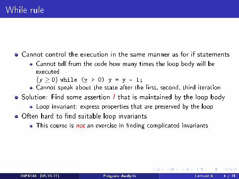
While rule

Cannot control the execution in the same manner as for if statements

Cannot tell from the code how many times the loop body will beexecuted{y ≥ 0} while (y > 0) y = y - 1;

Cannot speak about the state after the �rst, second, third iteration

Solution: Find some assertion I that is maintained by the loop body

Loop invariant: express properties that are preserved by the loop

Often hard to �nd suitable loop invariants

This course is not an exercise in �nding complicated invariants


While rule

{I ∧ B} S ; {I}{I} while (B) S ; {I ∧ ¬B}

Can use this rule to reason about the more general case:

{P} while (B) S {Q}

where

P need not be the loop invariant

Q need not match (I ∧ ¬B) syntacticallyCombine While rule with Consequence rule to prove:

Entry: P ⇒ I

Loop: {I ∧ B} S {I}Exit: I ∧ ¬B ⇒ Q


While rule: example

{0 ≤ n} k = 0; {k ≤ n} while (k < n) k = k+ 1; {k == n}

Composition rule splits a proof in two: assignment and loop.

Let k ≤ n be the loop invariant

Entry: k ≤ n follows from itself

Loop:k < n⇒ k + 1 ≤ n

{k ≤ n ∧ k < n} k = k+ 1 {k ≤ n}

Exit: (k ≤ n ∧ ¬(k < n))⇒ k == n


await statement

{P ∧ B} S; {Q}{P} < await (B); S;> {Q}

Remember that we are reasoning about safety properties

Termination is assumed

Noting bad will happen

The rule does not speak about waiting or progress


Concurrent execution

Assume two statements S1 og S2 such that:

{P1} < S1;> {Q1}{P2} < S2;> {Q2}

First attempt for a co..oc rule in PL:

{P1} < S1;> {Q1} {P2} < S2;> {Q2}{P1 ∧ P2} co < S1;> || < S2;> oc {Q1 ∧ Q2}

Example (Problem with this rule)

{x == 0} < x = x+ 1;> {x == 1}{x == 0} < x = x+ 2;> {x == 2}

{x == 0} co < x = x+ 1;> || < x = x+ 2;> oc {x == 1 ∧ x == 2}

but this conclusion is not true: the postcondition should be x == 3!


Interference problem

S1 : {x == 0} < x = x+ 1;> {x == 1}S2 : {x == 0} < x = x+ 2;> {x == 2}

The execution of S2 interferes with the pre- and postconditions for S1The assertion x == 0 need not hold when S1 starts execution

The execution of S1 interferes with the pre- and postconditions for S2The assertion x == 0 need not hold when S2 starts execution

Solution: weaken the assertions to account for the other process:

S1 : {x == 0 ∨ x == 2} < x = x+ 1;> {x == 1 ∨ x == 3}S2 : {x == 0 ∨ x == 1} < x = x+ 2;> {x == 2 ∨ x == 3}


Interference problem

Now we can try to apply the rule:

{x == 0 ∨ x == 2} < x = x+ 1;> {x == 1 ∨ x == 3}{x == 0 ∨ x == 1} < x = x+ 2;> {x == 2 ∨ x == 3}{PRE} co < x = x+ 1;> || < x = x+ 2;> oc {POST}

where:

PRE : (x == 0 ∨ x == 2) ∧ (x == 0 ∨ x == 1)POST : (x == 1 ∨ x == 3) ∧ (x == 2 ∨ x == 3)

which gives:

{x == 0} co < x = x+ 1;> || < x = x+ 2;> oc {x == 3}


Concurrent execution

Assume {Pi} Si {Qi} for all S1, . . . , Sn

{Pi} Si; {Qi} are interference free

{P1 ∧ . . . ∧ Pn} co S1; || . . . ||Sn; oc {Q1 ∧ . . . ∧ Qn}

Critical conditions are assertions outside critical sections (Pi ,Qi )

Interference freedom: The value of a critical condition is not changed

by execution of other processes


Interference freedom

Interference freedom

{C ∧ pre(S)} S {C}

C : critical condition

S : statement in some other process with precondition pre(S)

The critical condition �survives� execution of the the other process

{P1} S1; {Q1} {P2} S2; {Q2}{P1 ∧ P2} co S1; ||S2; oc {Q1 ∧ Q2}

Four interference requirements:

{P2 ∧ P1} S1 {P2} {P1 ∧ P2} S2 {P1}{Q2 ∧ P1} S1 {Q2} {Q1 ∧ P2} S2 {Q1}


Avoiding interference: Weakening assertions

S1 : {x == 0} < x = x+ 1;> {x == 1}S2 : {x == 0} < x = x+ 2;> {x == 2}

Here we have interference, for instance the precondition of S1 is not

maintained by execution of S2:

{(x == 0) ∧ (x == 0)} x = x+ 2; {x == 0}

is not true

However, after weakening:

S1 : {x == 0 ∨ x == 2} < x = x+ 1;> {x == 1 ∨ x == 3}S2 : {x == 0 ∨ x == 1} < x = x+ 2;> {x == 2 ∨ x == 3}

{(x == 0 ∨ x == 2) ∧ (x == 0 ∨ x == 1)} x = x+ 2 {x == 0 ∨ x == 2}

(Correspondingly for the other three critical conditions)


Avoiding interference: Disjoint variables

Read set: variables referred to by a process

Write set: variables written to by a process

Reference set: variables referred to by conditions in a proof of the

process

No interference if:

Write set of S1 is disjoint from reference set of S2

Write set of S2 is disjoint from reference set of S1

However, variables in a critical condition of one process will often be

among the write variables of another


Avoiding interference: Global invariants

Some condition that only refers to global (shared) variables

Holds initially

Preserved by all assignments

We avoid interference if critical conditions are on the form {I ∧ L} where:I is a global invariant

L only refers to local variables of the considered process


Avoiding interference: Synchronization

Hide critical conditions

MUTEX to critical sections

co . . . ; S ; . . . || . . . ; S1; {C}S2; . . . oc

S might interfere with C

Hide the critical condition by a critical region:

co . . . ; S ; . . . || . . . ;<S1; {C}S2;> . . . oc


Example: Producer/ consumer synchronization

Let Producer be a process that delivers data to a Consumer process

PC : c ≤ p ≤ c + 1 ∧ a[0 : n − 1] == A[0 : n − 1] ∧(p == c + 1)⇒ (buf == A[p − 1])

Let PC be a global invariant of the program:

int buf, p = 0, c = 0;

process Producer { process Consumer {

int a[n]; int b[n];

while (p < n) { while (c < n) {

< await (p == c) ; > < await (p > c) ; >

buf = a[p] b[c] = buf

p = p+1; c = c+1;

} }

} }


Example: Producer


process Producer {

int a[n];

{IP : PC ∧ p <= n} // loop invariant

while (p < n) {

{PC ∧ p < n}

< await (p == c); >

{PC ∧ p < n ∧ p == c}

buf = a[p];

{PC ∧ p < n ∧ p == c ∧ buf == A[p]}

p = p + 1;

{IP}

}

{PC ∧ p == n} // exit loop

}


Example: Producer


process Producer {

int a[n];


while (p < n) { {PC ∧ p < n}< await (p == c); >

{PC ∧ p < n ∧ p == c}

buf = a[p];

{PC ∧ p < n ∧ p == c ∧ buf == A[p]}

p = p + 1;

{IP}

}


}


Example: Producer


process Producer {

int a[n];


while (p < n) { {PC ∧ p < n}< await (p == c); > {PC ∧ p < n ∧ p == c}buf = a[p];

{PC ∧ p < n ∧ p == c ∧ buf == A[p]}

p = p + 1;

{IP}

}


}


Example: Producer


process Producer {

int a[n];


while (p < n) { {PC ∧ p < n}< await (p == c); > {PC ∧ p < n ∧ p == c}buf = a[p]; {PC ∧ p < n ∧ p == c ∧ buf == A[p]}p = p + 1;

{IP}

}


}


Example: Producer


process Producer {

int a[n];


while (p < n) { {PC ∧ p < n}< await (p == c); > {PC ∧ p < n ∧ p == c}buf = a[p]; {PC ∧ p < n ∧ p == c ∧ buf == A[p]}p = p + 1; {IP}

}


}


Example: Producer


process Producer {

int a[n];


while (p < n) { {PC ∧ p < n}< await (p == c); > {PC ∧ p < n ∧ p == c}buf = a[p]; {PC ∧ p < n ∧ p == c ∧ buf == A[p]}p = p + 1; {IP}

} {PC ∧ p == n} // exit loop

}


Example: Consumer


process Consumer {

int b[n];

{IC : PC ∧ c <= n ∧ b[0 : c − 1] == A[0 : c − 1]} // loop invariant

while (c < n) {

{IC ∧ c < n}

< await (p > c) ; >

{IC ∧ c < n ∧ p > c}

b[c] = buf;

{IC ∧ c < n ∧ p > c ∧ b[c] == A[c]}

c = c + 1;

{IC}

}

{IC ∧ c == n} # exit loop

}


Example: Consumer


process Consumer {

int b[n];


while (c < n) { {IC ∧ c < n}< await (p > c) ; >

{IC ∧ c < n ∧ p > c}

b[c] = buf;

{IC ∧ c < n ∧ p > c ∧ b[c] == A[c]}

c = c + 1;

{IC}

}


}


Example: Consumer


process Consumer {

int b[n];


while (c < n) { {IC ∧ c < n}< await (p > c) ; > {IC ∧ c < n ∧ p > c}b[c] = buf;

{IC ∧ c < n ∧ p > c ∧ b[c] == A[c]}

c = c + 1;

{IC}

}


}


Example: Consumer


process Consumer {

int b[n];


while (c < n) { {IC ∧ c < n}< await (p > c) ; > {IC ∧ c < n ∧ p > c}b[c] = buf; {IC ∧ c < n ∧ p > c ∧ b[c] == A[c]}c = c + 1;

{IC}

}


}


Example: Consumer


process Consumer {

int b[n];


while (c < n) { {IC ∧ c < n}< await (p > c) ; > {IC ∧ c < n ∧ p > c}b[c] = buf; {IC ∧ c < n ∧ p > c ∧ b[c] == A[c]}c = c + 1; {IC}

}


}


Example: Consumer


process Consumer {

int b[n];


while (c < n) { {IC ∧ c < n}< await (p > c) ; > {IC ∧ c < n ∧ p > c}b[c] = buf; {IC ∧ c < n ∧ p > c ∧ b[c] == A[c]}c = c + 1; {IC}

} {IC ∧ c == n} # exit loop

}


Example: Producer/Consumer

The �nal state of the program satis�es:

PC ∧ p == n ∧ IC ∧ c == n

which ensures that all elements in a are received and occur in the same

order in b

Interference freedom is ensured by the global invariant and await

statements

If we combine the two assertions after the await statements, we get:

PC ∧ p < n ∧ p == c ∧ IC ∧ c < n ∧ p > c

which gives false!

At any time, only one process can be after the await statement!


Monitor Invariant

monitor name {

monitor variable # shared global variable

initialization # for the monitor's procedures

procedures

}

A monitor invariant (I ) is used to describe the monitor's inner state

Express relationship between monitor variables

Maintained by execution of procedures:

Must hold after initializationMust hold when a procedure terminatesMust hold when we suspend execution due to a call to wait

Can assume that the invariant holds after wait and when a procedurestarts

Should be as strong as possible!


Axioms for Signal and Continue (1)

Assume that the monitor invariant I and predicate P does not mention cv.

Then we can set up the following axioms:

{I} wait(cv) {I}{P} signal(cv) {P} for arbitrary P

{P} signal_all(cv) {P} for arbitrary P


Monitor solution to reader/writer problem

Veri�cation of the invariant over request_read

I : (nr == 0 ∨ nw == 0) ∧ nw ≤ 1

procedure request_read() {

{I}

while (nw > 0) {

{I ∧ nw > 0}{I}

wait(oktoread);

{I}

}

{I ∧ nw == 0}

nr = nr + 1;

{I}

}

(I ∧ nw > 0)⇒ I

(I ∧ nw == 0)⇒ Inr ←(nr+1)




I : (nr == 0 ∨ nw == 0) ∧ nw ≤ 1


{I}while (nw > 0) {

{I ∧ nw > 0}{I}

wait(oktoread);

{I}

}

{I ∧ nw == 0}

nr = nr + 1;

{I}}

(I ∧ nw > 0)⇒ I

(I ∧ nw == 0)⇒ Inr ←(nr+1)




I : (nr == 0 ∨ nw == 0) ∧ nw ≤ 1


{I}while (nw > 0) {

{I ∧ nw > 0}

{I} wait(oktoread); {I}}

{I ∧ nw == 0}

nr = nr + 1;

{I}}

(I ∧ nw > 0)⇒ I

(I ∧ nw == 0)⇒ Inr ←(nr+1)




I : (nr == 0 ∨ nw == 0) ∧ nw ≤ 1


{I}while (nw > 0) { {I ∧ nw > 0}


{I ∧ nw == 0}

nr = nr + 1;

{I}}

(I ∧ nw > 0)⇒ I

(I ∧ nw == 0)⇒ Inr ←(nr+1)




I : (nr == 0 ∨ nw == 0) ∧ nw ≤ 1


{I}while (nw > 0) { {I ∧ nw > 0}


{I ∧ nw == 0}nr = nr + 1;

{I}}

(I ∧ nw > 0)⇒ I

(I ∧ nw == 0)⇒ Inr ←(nr+1)



Assume that the invariant can mention the number of processes in the

queue to a condition variable.

Let #cv be the number of processes waiting in the queue to cv .

The test empty(cv) is then identical to #cv == 0

wait(cv) is modelled as an extension of the queue followed by processor

release:

wait(cv) :

{?}

#cv = #cv + 1;

{I}

sleep

{I}

by assignment axiom:

wait(cv) : {I#cv ←(#cv+1)} #cv = #cv + 1; {I} sleep{I}








release:

wait(cv) :

{?}

#cv = #cv + 1;

{I}

sleep{I}










release:

wait(cv) :

{?}

#cv = #cv + 1; {I} sleep{I}










release:

wait(cv) : {?} #cv = #cv + 1; {I} sleep{I}





signal(cv) can be modelled as a reduction of the queue, if the queue is not

empty:

signal(cv) :

{?}

if (#cv != 0) #cv = #cv − 1

{P}

signal(cv) : {((#cv == 0)⇒ P) ∧ ((#cv 6= 0)⇒ P#cv ←(#cv−1))}if (#cv != 0) #cv = #cv − 1

{P}

signal_all(cv):

{P#cv ←0}

#cv = 0

{P}




empty:

signal(cv) :

{?}

if (#cv != 0) #cv = #cv − 1 {P}


{P}

signal_all(cv):

{P#cv ←0}

#cv = 0

{P}




empty:

signal(cv) : {?} if (#cv != 0) #cv = #cv − 1 {P}


{P}

signal_all(cv):

{P#cv ←0}

#cv = 0

{P}




empty:



{P}

signal_all(cv):

{P#cv ←0}

#cv = 0 {P}




empty:



{P}

signal_all(cv): {P#cv ←0} #cv = 0 {P}



Together this gives:

{I#cv ←(#cv+1)} wait(cv) {I}{((#cv == 0)⇒ P) ∧ ((#cv 6= 0)⇒ P#cv ←(#cv−1))} signal(cv) {P}

{P#cv ←0} signal_all(cv) {P}

If we know that #cv 6= 0 whenever we signal, then the axiom for

signal(cv) be simpli�ed to:

{P#cv ←(#cv−1)} signal(cv) {P}

Note! #cv is not allowed in statements!

Only used for reasoning


Example: FIFO semaphore veri�cation (1)

monitor FIFO_semaphore {

int s = 0; # value of semaphore

cond pos; # signalled only when s>0

procedure Psem() {

if (s==0)

wait(pos);

else

s = s-1;

}

procedure Vsem() {

if empty(pos)

s=s+1;

else

signal(pos);

}

}

Consider the following monitor invariant:

s ≥ 0 ∧ (s > 0⇒ #pos == 0)

No process is waiting if the semaphore value is positive



I : s ≥ 0 ∧ (s > 0⇒ #pos == 0)

procedure Psem() {

{I}

if (s==0)

{I ∧ s == 0}{I#pos←(#pos+1)}

wait(pos);

{I}

else

{I ∧ s 6= 0}{Is←(s−1)}

s = s-1;

{I}{I}

}



I : s ≥ 0 ∧ (s > 0⇒ #pos == 0)

procedure Psem() {

{I}if (s==0)

{I ∧ s == 0}{I#pos←(#pos+1)}

wait(pos);

{I}

else

{I ∧ s 6= 0}{Is←(s−1)}

s = s-1;

{I}{I}

}



I : s ≥ 0 ∧ (s > 0⇒ #pos == 0)

procedure Psem() {

{I}if (s==0)

{I ∧ s == 0}{I#pos←(#pos+1)}

wait(pos);

{I}

else

{I ∧ s 6= 0}{Is←(s−1)}

s = s-1;

{I}

{I}}



I : s ≥ 0 ∧ (s > 0⇒ #pos == 0)

procedure Psem() {

{I}if (s==0) {I ∧ s == 0}

{I#pos←(#pos+1)}

wait(pos);

{I}

else {I ∧ s 6= 0}

{Is←(s−1)}

s = s-1;

{I}

{I}}



I : s ≥ 0 ∧ (s > 0⇒ #pos == 0)

procedure Psem() {

{I}if (s==0) {I ∧ s == 0}

{I#pos←(#pos+1)}

wait(pos); {I}else {I ∧ s 6= 0}

{Is←(s−1)}

s = s-1; {I}{I}}



I : s ≥ 0 ∧ (s > 0⇒ #pos == 0)

procedure Psem() {

{I}if (s==0) {I ∧ s == 0}{I#pos←(#pos+1)} wait(pos); {I}

else {I ∧ s 6= 0}

{Is←(s−1)}

s = s-1; {I}{I}}



I : s ≥ 0 ∧ (s > 0⇒ #pos == 0)

procedure Psem() {

{I}if (s==0) {I ∧ s == 0}{I#pos←(#pos+1)} wait(pos); {I}

else {I ∧ s 6= 0}{Is←(s−1)} s = s-1; {I}

{I}}



I : s ≥ 0 ∧ (s > 0⇒ #pos == 0)

This gives two proof obligations:

If branch:

(I ∧ s == 0)⇒ I#pos←(#pos+1)

s == 0 ⇒ s ≥ 0 ∧ (s > 0⇒ #pos + 1 == 0)s == 0 ⇒ s ≥ 0

Else branch:

(I ∧ s 6= 0) ⇒ Is←(s−1)(s > 0 ∧#pos == 0)⇒ s − 1 ≥ 0 ∧ (s − 1 ≥ 0⇒ #pos == 0)(s > 0 ∧#pos == 0)⇒ s > 0 ∧#pos == 0



I : s ≥ 0 ∧ (s > 0⇒ #pos == 0)

procedure Vsem() {

{I}

if empty(pos)

{I ∧#pos == 0}{Is←(s+1)}

s=s+1;

{I}

else

{I ∧#pos 6= 0}{I#pos←(#pos−1)}

signal(pos);

{I}{I}

}



I : s ≥ 0 ∧ (s > 0⇒ #pos == 0)

procedure Vsem() {

{I}if empty(pos)

{I ∧#pos == 0}{Is←(s+1)}

s=s+1;

{I}

else

{I ∧#pos 6= 0}{I#pos←(#pos−1)}

signal(pos);

{I}

{I}}



I : s ≥ 0 ∧ (s > 0⇒ #pos == 0)

procedure Vsem() {

{I}if empty(pos) {I ∧#pos == 0}

{Is←(s+1)}

s=s+1;

{I}

else {I ∧#pos 6= 0}

{I#pos←(#pos−1)}

signal(pos);

{I}

{I}}



I : s ≥ 0 ∧ (s > 0⇒ #pos == 0)

procedure Vsem() {

{I}if empty(pos) {I ∧#pos == 0}

{Is←(s+1)}

s=s+1; {I}else {I ∧#pos 6= 0}


signal(pos); {I}{I}}



I : s ≥ 0 ∧ (s > 0⇒ #pos == 0)

procedure Vsem() {

{I}if empty(pos) {I ∧#pos == 0}{Is←(s+1)}s=s+1; {I}

else {I ∧#pos 6= 0}


signal(pos); {I}{I}}



I : s ≥ 0 ∧ (s > 0⇒ #pos == 0)

procedure Vsem() {

{I}if empty(pos) {I ∧#pos == 0}{Is←(s+1)}s=s+1; {I}

else {I ∧#pos 6= 0}{I#pos←(#pos−1)} signal(pos); {I}

{I}}



I : s ≥ 0 ∧ (s > 0⇒ #pos == 0)

As above, this gives two proof obligations:

If branch:

(I ∧#pos == 0) ⇒ Is←(s+1)

(s ≥ 0 ∧#pos == 0)⇒ s + 1 ≥ 0 ∧ (s + 1 > 0⇒ #pos == 0)(s ≥ 0 ∧#pos == 0)⇒ s + 1 ≥ 0 ∧#pos == 0

Else branch:

(I ∧#pos 6= 0) ⇒ I#pos←(#pos−1)(s == 0 ∧#pos 6= 0)⇒ s ≥ 0 ∧ (s > 0⇒ #pos − 1 == 0)s == 0 ⇒ s ≥ 0


program analysis - uio.no fileprogram logic (pl) pl lets us express and prove properties about...

Documents