Profex User Manual

Version 3.9.0 Nicola DobelinMay 1, 2016

Contents

1. Introduction 5

2. Installation 62.1. Windows . . . . . . . . . . . . . . . . . . . . . . . . . . . . . . . . . . . . . . . . . . . . 6

2.1.1. Profex-BGMN bundle . . . . . . . . . . . . . . . . . . . . . . . . . . . . . . . . 62.2. Linux . . . . . . . . . . . . . . . . . . . . . . . . . . . . . . . . . . . . . . . . . . . . . . 6

2.2.1. Getting the source . . . . . . . . . . . . . . . . . . . . . . . . . . . . . . . . . . 72.2.2. Compiling from source code . . . . . . . . . . . . . . . . . . . . . . . . . . . . 7

2.3. Mac OS X . . . . . . . . . . . . . . . . . . . . . . . . . . . . . . . . . . . . . . . . . . . . 7

3. Setup 83.1. Automatic setup . . . . . . . . . . . . . . . . . . . . . . . . . . . . . . . . . . . . . . . . 8

3.1.1. Windows . . . . . . . . . . . . . . . . . . . . . . . . . . . . . . . . . . . . . . . . 83.1.2. Linux . . . . . . . . . . . . . . . . . . . . . . . . . . . . . . . . . . . . . . . . . . 83.1.3. Mac OS X . . . . . . . . . . . . . . . . . . . . . . . . . . . . . . . . . . . . . . . 9

3.2. Manual setup . . . . . . . . . . . . . . . . . . . . . . . . . . . . . . . . . . . . . . . . . 93.3. Using WINE on Linux . . . . . . . . . . . . . . . . . . . . . . . . . . . . . . . . . . . . 113.4. Structure, Device, and Preset Database . . . . . . . . . . . . . . . . . . . . . . . . . . . 11

3.4.1. Structure Template Files . . . . . . . . . . . . . . . . . . . . . . . . . . . . . . . 113.4.2. STR File Handling . . . . . . . . . . . . . . . . . . . . . . . . . . . . . . . . . . 123.4.3. Device Configuration Files . . . . . . . . . . . . . . . . . . . . . . . . . . . . . 133.4.4. Refinement Preset Files . . . . . . . . . . . . . . . . . . . . . . . . . . . . . . . 14

4. First steps 16

5. Main Window 185.1. User Interface Elements . . . . . . . . . . . . . . . . . . . . . . . . . . . . . . . . . . . 185.2. Dockable windows . . . . . . . . . . . . . . . . . . . . . . . . . . . . . . . . . . . . . . 19

5.2.1. Projects . . . . . . . . . . . . . . . . . . . . . . . . . . . . . . . . . . . . . . . . . 195.2.2. Plot options . . . . . . . . . . . . . . . . . . . . . . . . . . . . . . . . . . . . . . 215.2.3. Refinement protocol . . . . . . . . . . . . . . . . . . . . . . . . . . . . . . . . . 215.2.4. Global Parameters and GOALs . . . . . . . . . . . . . . . . . . . . . . . . . . . 215.2.5. Local Parameters . . . . . . . . . . . . . . . . . . . . . . . . . . . . . . . . . . . 225.2.6. Chemistry . . . . . . . . . . . . . . . . . . . . . . . . . . . . . . . . . . . . . . . 225.2.7. Context Help . . . . . . . . . . . . . . . . . . . . . . . . . . . . . . . . . . . . . 225.2.8. Convercence Progress . . . . . . . . . . . . . . . . . . . . . . . . . . . . . . . . 22

5.3. The Plot Area . . . . . . . . . . . . . . . . . . . . . . . . . . . . . . . . . . . . . . . . . 245.3.1. Central Data Area . . . . . . . . . . . . . . . . . . . . . . . . . . . . . . . . . . 255.3.2. Left Margin Area . . . . . . . . . . . . . . . . . . . . . . . . . . . . . . . . . . . 265.3.3. Bottom Margin Area . . . . . . . . . . . . . . . . . . . . . . . . . . . . . . . . . 265.3.4. Stacking Scans . . . . . . . . . . . . . . . . . . . . . . . . . . . . . . . . . . . . 28

5.4. Text Editors . . . . . . . . . . . . . . . . . . . . . . . . . . . . . . . . . . . . . . . . . . 285.4.1. Control File specific features . . . . . . . . . . . . . . . . . . . . . . . . . . . . 28

2

5.4.2. Control and Structure File specific features . . . . . . . . . . . . . . . . . . . . 305.5. Tool bars . . . . . . . . . . . . . . . . . . . . . . . . . . . . . . . . . . . . . . . . . . . . 315.6. Menu Structure . . . . . . . . . . . . . . . . . . . . . . . . . . . . . . . . . . . . . . . . 31

5.6.1. File . . . . . . . . . . . . . . . . . . . . . . . . . . . . . . . . . . . . . . . . . . . 315.6.2. Edit . . . . . . . . . . . . . . . . . . . . . . . . . . . . . . . . . . . . . . . . . . . 335.6.3. View . . . . . . . . . . . . . . . . . . . . . . . . . . . . . . . . . . . . . . . . . . 335.6.4. Project . . . . . . . . . . . . . . . . . . . . . . . . . . . . . . . . . . . . . . . . . 345.6.5. Run . . . . . . . . . . . . . . . . . . . . . . . . . . . . . . . . . . . . . . . . . . . 355.6.6. Results . . . . . . . . . . . . . . . . . . . . . . . . . . . . . . . . . . . . . . . . . 365.6.7. Instrument . . . . . . . . . . . . . . . . . . . . . . . . . . . . . . . . . . . . . . . 365.6.8. Window . . . . . . . . . . . . . . . . . . . . . . . . . . . . . . . . . . . . . . . . 375.6.9. Help . . . . . . . . . . . . . . . . . . . . . . . . . . . . . . . . . . . . . . . . . . 37

6. Preferences 386.1. General . . . . . . . . . . . . . . . . . . . . . . . . . . . . . . . . . . . . . . . . . . . . . 386.2. Text Editors . . . . . . . . . . . . . . . . . . . . . . . . . . . . . . . . . . . . . . . . . . 386.3. Graphs . . . . . . . . . . . . . . . . . . . . . . . . . . . . . . . . . . . . . . . . . . . . . 39

6.3.1. Fonts . . . . . . . . . . . . . . . . . . . . . . . . . . . . . . . . . . . . . . . . . . 406.3.2. Scan Styles . . . . . . . . . . . . . . . . . . . . . . . . . . . . . . . . . . . . . . . 40

6.4. BGMN . . . . . . . . . . . . . . . . . . . . . . . . . . . . . . . . . . . . . . . . . . . . . 406.4.1. Structure File Handling . . . . . . . . . . . . . . . . . . . . . . . . . . . . . . . 436.4.2. Limits . . . . . . . . . . . . . . . . . . . . . . . . . . . . . . . . . . . . . . . . . 446.4.3. Summary Table . . . . . . . . . . . . . . . . . . . . . . . . . . . . . . . . . . . . 44

6.5. Fullprof . . . . . . . . . . . . . . . . . . . . . . . . . . . . . . . . . . . . . . . . . . . . . 466.6. Reference Structures . . . . . . . . . . . . . . . . . . . . . . . . . . . . . . . . . . . . . 476.7. Chemical Composition . . . . . . . . . . . . . . . . . . . . . . . . . . . . . . . . . . . . 476.8. Text Blocks . . . . . . . . . . . . . . . . . . . . . . . . . . . . . . . . . . . . . . . . . . . 48

7. Adding and Removing Structure Files 497.1. Project organization . . . . . . . . . . . . . . . . . . . . . . . . . . . . . . . . . . . . . . 507.2. ,,Refinement Preset” . . . . . . . . . . . . . . . . . . . . . . . . . . . . . . . . . . . . . 51

7.2.1. Creating and using presets . . . . . . . . . . . . . . . . . . . . . . . . . . . . . 53

8. Exporting data 568.1. Graphs . . . . . . . . . . . . . . . . . . . . . . . . . . . . . . . . . . . . . . . . . . . . . 56

8.1.1. ASCII free format (XY) . . . . . . . . . . . . . . . . . . . . . . . . . . . . . . . . 568.1.2. ASCII HKL List (HKL) . . . . . . . . . . . . . . . . . . . . . . . . . . . . . . . . 578.1.3. Pixel image (PNG) . . . . . . . . . . . . . . . . . . . . . . . . . . . . . . . . . . 578.1.4. Gnuplot (GPL) . . . . . . . . . . . . . . . . . . . . . . . . . . . . . . . . . . . . 588.1.5. Grace plots (AGR) . . . . . . . . . . . . . . . . . . . . . . . . . . . . . . . . . . 588.1.6. Scalable vector graphics (SVG) . . . . . . . . . . . . . . . . . . . . . . . . . . . 588.1.7. Fityk Session (FIT) . . . . . . . . . . . . . . . . . . . . . . . . . . . . . . . . . . 59

8.2. Printing to PDF . . . . . . . . . . . . . . . . . . . . . . . . . . . . . . . . . . . . . . . . 608.3. Refinement results . . . . . . . . . . . . . . . . . . . . . . . . . . . . . . . . . . . . . . 60

8.3.1. CSV tables . . . . . . . . . . . . . . . . . . . . . . . . . . . . . . . . . . . . . . . 60

3

9. Chemical composition 62

10. Limits of Quantification and Detection 63

11. Profex-specific Control File Variables 69

12. Scan batch conversion 70

13. CIF and ICDD XML import 7113.1. Automatic conversion of thermal displacement parameters . . . . . . . . . . . . . . . 72

14. Instrument configurations 75

15. Scan File Handling 77

A. Bundle File Structure 84A.1. Windows . . . . . . . . . . . . . . . . . . . . . . . . . . . . . . . . . . . . . . . . . . . . 84A.2. Mac OS X . . . . . . . . . . . . . . . . . . . . . . . . . . . . . . . . . . . . . . . . . . . . 84A.3. Linux . . . . . . . . . . . . . . . . . . . . . . . . . . . . . . . . . . . . . . . . . . . . . . 85

Index 87

4

1. Introduction

Profex is a graphical user interface for Rietveld refinement of powder X-ray diffraction data withthe program BGMN [1]. It provides a large number of convenience features and facilitates the useof the BGMN Rietveld backend in many ways. Some of the program’s key features include:

• Support for a variety of raw data formats, including all major instrument manufacturers(Bruker / Siemens, PANalytical / Philips, Rigaku, Seifert / GE, and generic text formats)

• Export of diffraction patterns to various text formats (ASCII, Gnuplot scripts, Fityk scripts),pixel graphics (PNG), and vector graphics (SVG)

• Batch conversion of raw data scans

• Automatic control file creation and output file name management

• Conversion of CIF and ICDD PDF-4+ XML structure files to BGMN structure files

• Internal database for crystal structure files, instrument configuration files, and predefinedrefinement presets.

• Computation of chemical composition from refined crystal structures

• Batch refinement

• Export of refinement results to spread sheet files (CSV format)

• Context help for BGMN variables

• Syntax highlighting

• Enhanced text editors for structure and control file management and editing

• Generic support for FullProf.2k [2] as an alternative Rietveld backend to BGMN.

• And many more. . .

Profex runs on Windows, Linux, and Mac OS X operating systems and is available as free softwarelicensed under the GNU General Public License (GPL) version 2 or any later version. The latestversion of the program can be downloaded from [3]. This website provides the Profex sourcecode, bundles of Profex and BGMN for easy installation on Windows and Mac OS X (requiringzero configuration), and a default set of crystal structure and instrument configuration files.

5

2. Installation

2.1. Windows

2.1.1. Profex-BGMN bundle

Since Profex requires a Rietveld refinement backend, a bundle containing both Profex and BGMNis offered for download on the Profex website. Using the bundle is the preferred way of installa-tion if no previous installation is present on the computer. The directory and file structure of thebundle is shown in appendix ??. The software does not need installation. The downloaded archivecan be extracted to any location on the computer. Automatic configuration of Profex will be ableto locate the BGMN installation if the relative paths of the BGMNwin and Profex-3.9.0 folders aremaintained. Therefore, it is recommended to copy the entire bundle to the same location on thehard disk, as shown in Fig. 1. Follow these instructions to install BGMN and Profex:

1. Download Profex-BGMN-Bundle-3.9.0.zip from [3]

2. Extract the bundle to your harddisk (e. g. C:\Program Files)

3. Run Profex by executing the file profex.exe (e. g. C:\Program Files\Profex-BGMN-Bundle\Profex\profex.exe)

The file and directory structure of the bundle is explained in appendix A. Profex is also availablefor download without BGMN. This is the preferred way of installation if BGMN is already in-stalled on the computer, or if previous versions of Profex are to be upgraded. The Profex binaryarchive does not need installation. Extracting the archive to the local hard drive is sufficient.

If a previous version is installed on the same computer, using a new version will not interfere withthe existing installation. Old and new versions can be used at the same time, they will share theconfiguration options.

2.2. Linux

A binary archive of BGMN for Linux (i686) is available for download on the Profex website [3].Profex, however, must be compiled from source. It requires a C++ compiler environment and theQt toolkit version 5 to be installed [4], including header files. Qt version 5.4 or later is required.The following Qt 5 modules and header files must be installed:

widgets, xml, printsupport, sql, svg

Support for Bruker BRML raw data files requires the 3rd party libraries zlib [5] and QuaZip [6].Both libraries are included in the Profex source code archive and linked statically into the binaryin order to avoid version conflicts with system-wide installed libraries linked against Qt version4.

6

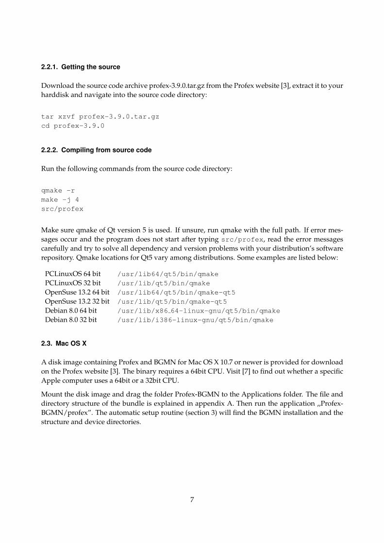
2.2.1. Getting the source

Download the source code archive profex-3.9.0.tar.gz from the Profex website [3], extract it to yourharddisk and navigate into the source code directory:

tar xzvf profex-3.9.0.tar.gzcd profex-3.9.0

2.2.2. Compiling from source code

Run the following commands from the source code directory:

qmake -rmake -j 4src/profex

Make sure qmake of Qt version 5 is used. If unsure, run qmake with the full path. If error mes-sages occur and the program does not start after typing src/profex, read the error messagescarefully and try to solve all dependency and version problems with your distribution’s softwarerepository. Qmake locations for Qt5 vary among distributions. Some examples are listed below:

PCLinuxOS 64 bit /usr/lib64/qt5/bin/qmakePCLinuxOS 32 bit /usr/lib/qt5/bin/qmakeOpenSuse 13.2 64 bit /usr/lib64/qt5/bin/qmake-qt5OpenSuse 13.2 32 bit /usr/lib/qt5/bin/qmake-qt5Debian 8.0 64 bit /usr/lib/x86 64-linux-gnu/qt5/bin/qmakeDebian 8.0 32 bit /usr/lib/i386-linux-gnu/qt5/bin/qmake

2.3. Mac OS X

A disk image containing Profex and BGMN for Mac OS X 10.7 or newer is provided for downloadon the Profex website [3]. The binary requires a 64bit CPU. Visit [7] to find out whether a specificApple computer uses a 64bit or a 32bit CPU.

Mount the disk image and drag the folder Profex-BGMN to the Applications folder. The file anddirectory structure of the bundle is explained in appendix A. Then run the application ,,Profex-BGMN/profex”. The automatic setup routine (section 3) will find the BGMN installation and thestructure and device directories.

7

Profex-BGMN-Bundle-3.9.0.zipBGMNwin

BGMN.EXE...

Profex-3.9.0profex.exe...Structures

*.strDevices

*.geq / *.ger

*.sav / *.tplPresets

*.pfp

(a) Structure of the bundle archive.

C:\Program Files\Profex-BGMNBGMNwin

BGMN.EXE...

Profex-3.9.0profex.exe...Structures

*.strDevices

*.geq / *.ger

*.sav / *.tplPresets

*.pfp

(b) Structure on the hard disk.

Figure 1: When extracting the Profex-BGMN-Bundle to the hard disk, automatic setup will only besuccessful if the BGMNwin and Profex-3.9.0 directories are copied to the same location.

3. Setup

3.1. Automatic setup

When starting Profex for the first time, the program will try to locate the BGMN installation di-rectory and structure and device database directories automatically. Automatic configuration willalso be executed later if the configured paths are invalid. It is therefore possible to force automaticsetup later by deleting the paths to BGMN and the database directories in the preferences dialog.Automatic setup is platform specific. The locations scanned automatically are listed below.

3.1.1. Windows

Three directories named ,,Structures”, ,,Devices”, and ,,Presets” are expected to be located in thedirectory of ,,profex.exe”. ,,BGMN.EXE” is expected to be found in a directory called BGMNwinstored next to the parent directory of ,,profex.exe”. In other words, automatic setup on Windowswill work if BGMN and Profex directories are organized as shown in Figure 1.

3.1.2. Linux

On Linux, a list of directories is scanned for the executable file ,,bgmn”. Scanning will stop at thefirst match. The directories are scanned in the following order:

1. /home/<user>/BGMN/

2. /home/<user>/BGMNwin/

8

3. /opt/bgmnwin/

4. /opt/bgmn/

5. /opt/BGMNwin/

6. /usr/bin/

7. /usr/local/bin/

Directories named ,,Structures” ,,Devices”, and ,,Presets” will be searched in the following orderat:

1. /opt/BGMN-Templates/Structures/opt/BGMN-Templates/Devices/opt/BGMN-Templates/Presets

2. /home/<user>/Documents/BGMN-Templates/Structures/home/<user>/Documents/BGMN-Templates/Devices/home/<user>/Documents/BGMN-Templates/Presets

3. /home/<user>/BGMN-Templates/Structures/home/<user>/BGMN-Templates/Devices/home/<user>/BGMN-Templates/Presets

3.1.3. Mac OS X

On Mac OS X the BGMN installation and Structures and Devices directories will be scanned rela-tive to the path of the Profex application bundle. Profex expects to find the following files, startingat the position of the Profex application bundle:

• <location of profex.app>/../BGMNwin/bgmn

• <location of profex.app>/../BGMN-Templates/Structures

• <location of profex.app>/../BGMN-Templates/Devices

• <location of profex.app>/../BGMN-Templates/Presets

3.2. Manual setup

The following sections describe how to configure Profex to find the BGMN backend, as well asthe structure, device, and preset database directories manually. There are some scenarios whenautomatic setup will fail and the backend and database directories are not found, or when theautomatic configuration is not desired:

• if only Profex was downloaded instead of a Profex-BGMN bundle

9

(a) Set the default project type to BGMN. (b) Select the BGMN executable files (red), as well asstructure, device, and preset database directories(green).

Figure 2: Manual configuration of the BGMN backend in Profex.

• if the Profex and BGMN folders from the bundle were not copied to the same location on theharddisk

• if other structure and device repositories will be used than the ones provided with the bun-dle. E. g. centrally stored on a network shared drive, or from a previous installation.

• on Linux no bundles are available

In these cases, manual configuration is necessary. Follow these instructions to set up Profex man-ually:

1. Run Profex and go to ,,Edit→ Preferences . . . ”.

2. On the page ,,General” set the ,,Default Project Type” to ,,BGMN” (Fig. 2).

3. Go to page ,, BGMN” and check the configuration of ,,BGMN Backend”. If auto-detectionwas successful, the lines for executable files and files directories are not empty (Fig. 2).

4. If the lines are empty, click the button on the right of each line and navigate to the corre-sponding executable file. The file names depend on the operating system. On Windows, thefiles are called BGMN.EXE, MAKEGEQ.EXE, GEOMET.EXE, and OUTPUT.EXE. On Linux andMac OS X these files are called bgmn, makegeq, geomet, and output.

5. Verify the location of the Structure, Device, and Preset directories. If they are empty or pointto the wrong location, click on the button on the right and select the correct directories.

10

3.3. Using WINE on Linux

Profex supports running the Windows version of BGMN on Linux using WINE. In that case, a,,BGMNwin” directory from a Windows installation can be copied to any location on a Linuxsystem. The executable files of the BGMN backend will then be called BGMN.EXE, MAKEGEQ.EXE,GEOMET.EXE, OUTPUT.EXE, and GERTEST.EXE. Checking the box ,,Run in WINE” and enteringthe WINE executable in the configuration dialog (Fig. 2), which is usually /usr/bin/wine, willlet Profex call the BGMN backend in WINE. However, for performance reasons it is recommendedto use the native Linux version of BGMN if available.

3.4. Structure, Device, and Preset Database

Profex supports databases for crystal structures, device configurations, and refinement presets forthe BGMN backend. These databases are directories containing template files. Official Profex-BGMN bundles usually contain default template files for structures and devices. The location ofthese directories can be chosen freely. For example, installations on several computers can accessstructures, device files, and presets stored on a network share and maintained centrally. In thatcase, new structure files, device configurations, or presets will immediately become available toall users using the same database directories. Write access is not required for normal use, only formaintenance. Configuration (automatic or manual) is explained in section 2. Several structure filedirectories can be specified, but only one directory for device and preset files, respectively.

3.4.1. Structure Template Files

Template files for crystal structures are normal BGMN structure files (*.str) stored at a centralplace in the ,,Structures” database directory. When appending a structure file from the database toa refinement using Profex’s ,,Add / Remove Phase” dialog, the file will be copied to the locationof the XRD scan. The original file will never be modified.

The following information is relevant when creating new structure files:

• Use the file extension *.str, other files will be ignored by Profex

• Profex will display the name given after the keyword ,,PHASE=” in the ,,Add / RemovePhase” dialog.

• It is recommended to add further information, e. g. an original database code (PDF, AMCSD,COD) after a comment sign (//) trailing the ,,PHASE=” keyword (see following example).This text will be shown as a comment in the ,,Add / Remove Phase” dialog.

The following lines show an example of the file ,,lime.str”.

11

Figure 3: Profex allows to modify structure files automatically to apply custom profile functionsand goals.

PHASE=CaO // 04-007-9734SpacegroupNo=225 HermannMauguin=F4/m-32/m //PARAM=A=0.4819_0.4771ˆ0.4867 //RP=4 k1=0 k2=0 B1=ANISOˆ0.01 GEWICHT=SPHAR2 //GOAL=GrainSize(1,1,1) //GOAL:CaO=GEWICHT*ifthenelse(ifdef(d),exp(my*d*3/4),1)E=CA+2 Wyckoff=a x=0.0000 y=0.0000 z=0.0000 TDS=0.00350000E=O-2 Wyckoff=b x=0.5000 y=0.5000 z=0.5000 TDS=0.00440000

3.4.2. STR File Handling

Depending on where structure files are obtained from (created manually, exported from databases,converted, downloaded, shared with others) they may contain different profile parameters RP, B1,k1, k2, GEWICHT etc. Altering these files in the structure file database will also affect other usersaccessing the same database, and may thus not be desired. Profex offers a feature to modify thestructure files while copying them from the database to the working directory. Choose ,,Edit →Preferences→ BGMN→ Structure File Handling” to access the settings (Fig. 3). The individualoptions on this page are explained in more detail in section 6.4.1.

12

3.4.3. Device Configuration Files

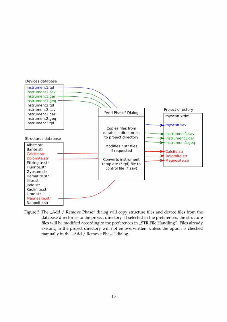
For each device configuration Profex expects to find four different files in the device databasedirectory. These file names are supposed to have the same file name, but different file extensions(Fig. 5):

*.sav Containing the description of the device configuration. To be processed with GEOMET.

*.ger Containing the raytraced profile shape. To be processed with MAKEGEQ.

*.geq Containing the interpolated profile.

*.tpl A sample *.sav control file for the refinement, not containing any file names or phases (op-tional).

The *.tpl file is specific to Profex, all other files will be required by BGMN. The *.tpl file can be anyexisting refinement control file, but all output file names (LIST=, OUTPUT=, DIAGRAMM=), all scanfile names VAL[n]=, and all structure file names STRUC[n]= should be empty. *.tpl files allow toadd goals, calculations, numbers of threads and similar customizations, which will be applied bydefault when creating a new file set from the database. An example is shown below. All devicefile names, structure files, scan files, and the various output files will be filled in automaticallyby Profex. The automatic processes running in the background when using the ,,Add / RemovePhase” dialog are illustrated in Fig. 5. More information on the ,,Add / Remove Phase” dialogcan be found in section 7.

% Theoretical instrumental functionVERZERR=% WavelengthLAMBDA=CU% Phases% Measured dataVAL[1]=% Minimum Angle (2theta)% WMIN=10% Maximum Angle (2theta)% WMAX=60% Result list outputLIST=% Peak list outputOUTPUT=% Diagram outputDIAGRAMM=% Global parameters for zero point and sample displacementEPS1=0PARAM[1]=EPS2=0_-0.001ˆ0.001betaratio=0

13

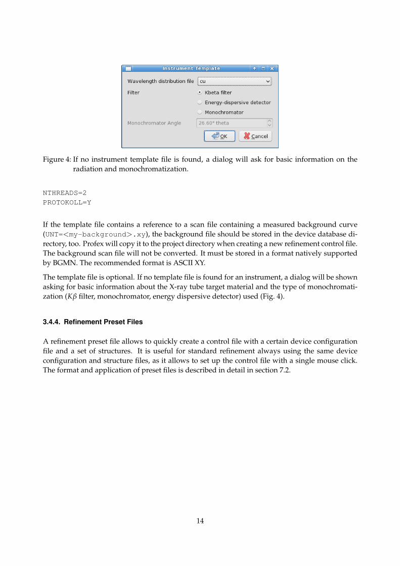
Figure 4: If no instrument template file is found, a dialog will ask for basic information on theradiation and monochromatization.

NTHREADS=2PROTOKOLL=Y

If the template file contains a reference to a scan file containing a measured background curve(UNT=<my-background>.xy), the background file should be stored in the device database di-rectory, too. Profex will copy it to the project directory when creating a new refinement control file.The background scan file will not be converted. It must be stored in a format natively supportedby BGMN. The recommended format is ASCII XY.

The template file is optional. If no template file is found for an instrument, a dialog will be shownasking for basic information about the X-ray tube target material and the type of monochromati-zation (Kβ filter, monochromator, energy dispersive detector) used (Fig. 4).

3.4.4. Refinement Preset Files

A refinement preset file allows to quickly create a control file with a certain device configurationfile and a set of structures. It is useful for standard refinement always using the same deviceconfiguration and structure files, as it allows to set up the control file with a single mouse click.The format and application of preset files is described in detail in section 7.2.

14

Structures database

Albite.strBarite.strCalcite.strDolomite.strEttringite.strFluorite.strGypsum.strHematite.strIllite.strJade.strKaolinite.strLime.strMagnesite.strNahpoite.str

Devices database

Instrument1.tplInstrument1.savInstrument1.gerInstrument1.geqInstrument2.tplInstrument2.savInstrument2.gerInstrument2.geqInstrument3.tpl

Project directory

myscan.xrdml

myscan.sav

Instrument1.savInstrument1.gerInstrument1.geq

Calcite.strDolomite.strMagnesite.str

Copies files fromdatabase directoriesto project directory

Modifies *.str filesif requested

Converts instrumenttemplate (*.tpl) file to

control file (*.sav)

"Add Phase" Dialog

Figure 5: The ,,Add / Remove Phase” dialog will copy structure files and device files from thedatabase directories to the project directory. If selected in the preferences, the structurefiles will be modified according to the preferences in ,,STR File Handling”. Files alreadyexisting in the project directory will not be overwritten, unless the option is checkedmanually in the ,,Add / Remove Phase” dialog.

15

4. First steps

When Profex and BGMN have been installed and configured correctly as described in sections 2and 3, and at least one device configuration and structure file has been stored in the databases(section 3.4), the program is ready for a first refinement:

1. Click ,,File→ Open Graph. . . ”, or alternatively press Ctrl+G or the corresponding button inthe main tool bar.

2. In the opening file dialog set the file format at the bottom to the format of your raw scanfile, and open the file. See Tab. 1 for supported file formats. If a format is not supported, orsupport is broken, other software such as PowDLL [11] is required to convert the scan to aformat supported by Profex.

3. The scan will be loaded as a new project.1

4. Double click on the strongest peak or select a reference structure from the reference structuredropdown menu to identify your main phase.

5. Click ,,Edit → Add / Remove Phase. . . ”, or press F8 or the corresponding button in theproject tool bar create a control file. The dialog shown in Fig. 12 will be shown.

6. Select your instrument configuration from the dropdown menu, your phase from the struc-tures list (it may be pre-selected), and verify that the option ,,Generate default control file”is active. Then click ,,OK”.

7. Click ,,Run→ Run Refinement. . . ”, press F9, or click the corresponding button in the refine-ment tool bar to start the refinement.

8. Wait for the refinement to complete.

9. If more phases are present, repeat steps 4–7, but make sure the option ,,Generate defaultcontrol file” is not active anymore.

10. If the refinement is complete, click ,,File→ Export Global Parameters and GOALs”, or pressCtrl+E or the corresponding button in the project tool bar to export the results to a CSV file.

11. Optionally, also click ,,File→ Export Local Parameters and GOALs”, or press Shift+Ctrl+Eor the corresponding button in the project tool bar to export the local results to a CSV file.

The exported CSV files can be opened in a spreadsheet program such as Microsoft Excel, Libre-Office Calc, or Softmaker PlanMaker. Specify the semicolon ,,;” as field separator and use thespreadsheet program’s sort feature to sort the parameters as needed.

1At the first start of the program, all reference structures in the structure database directory will be indexed. Depend-ing on the number of files and the speed of the computer, this may take up to several minutes. A progress dialog isshown while indexing is in progress.

16

Table 1: Data file formats supported for import by Profex. Level of support (LoS): A = full sup-port based on the file format specification, including multi-range files; B = good support,reverse-engineered; C = basic support, reverse engineered.

Manufacturer Extension File format Version LoS

Bruker *.raw Binary V1, V2, V3, V4 ABruker *.brml XML Compressed archive BBruker *.brml XML Single XML file with XML data

containerB

Bruker *.brml XML Single XML file with binarydata container

B

PANalytical *.xrdml XML 1.0 - 1.5 APhilips *.rd Binary - CPhilips *.udf ASCII - CSeifert/FPM *.val ASCII - BRigaku *.bin Binary - CRigaku *.dat, *.rig, *.dif ASCII - CRigaku *.raw Binary - CMDI Jade *.xml XML - CMDI Jade *.dif ASCII - CSTOE *.pro ASCII - CSTOE *.raw Binary - CGeneric *.xy ASCII Field separators: ; : , space tab

Comment signs: ! % & #A

BGMN *.dia ASCII - AFullprof.2k *.prf ASCII Only PRF=3 AFullprof.2k *.dat ASCII Only INS=10 A

17

5. Main Window

The program’s main window features a menu bar and several tool bars to access all functions andsettings (Fig. 6). The central area of the main window is occupied by the plot area, and optionallyone or several text editors, which are accessible by tabs at the top of the plot area. The plot areacannot be closed, but text editors can be closed by clicking the close button on their tab.

The central area is surrounded by several dockable windows showing additional information andgiving access to more features. These dockable windows can be closed and opened from the,,Window” menu. They can also be re-arranged (Fig. 7) by clicking on the title bar showing thewindow’s name, and dragging it to another location. Dockable windows can be stacked on top ofeach other to hide less frequently used windows, or detached from the main window, e. g. to beplaced on another screen, or closed.

5.1. User Interface Elements

The following list explains the elements of the user interface shown in Fig. 6 in more detail.

1 Menu bar gives access to most features, as well as the program’s preferences. All menu itemsare discussed in section 5.6.

2 Main tool bar gives access to file operating features such as opening, saving, etc.

3 Project tool bar gives access to project related functions, such as opening/closing structurefiles, exporting results, adding/removing phases etc.

4 Refinement tool bar gives access to starting/stopping refinements or batch refinements.

5 Reference structure tool bar allows to select reference structures to display hkl indices, as wellas to start scanning and indexing new structure files. See section 5.5 for more information.

6 Plot area displays raw or refined scans, and opens text editors for control files, results files,structure files, or generic text files.

7 Projects window lists all open projects and the refinement status. Selecting a project from thislist will show it in the central plot area.

8 Plot options lists all scans loaded in the plot area. The ,,Show” checkbox can be used toshow/hide certain scans to customize the appearance of the plot.

9 Refinement protocol shows output generated by the refinement backend.

10 Global Parameters and GOALs shows a summary table of refined global parameters. ListingEPS parameters can be configured in the program’s preferences dialog.

11 Local Parameters and GOALs shows a summary table of refined local parameters. The pa-rameters shown here can be customized in the program’s preferences dialog.

12 Context help shows the context help text when pressing ,,F1” on a keyword in a control file.

18

13 Chemical composition shows the bulk chemical composition of all crystalline phases, calcu-lated from refined crystal structures and phase quantities.

14 Status bar shows various information such as mouse cursor coordinates on the graph, and thewavelength used to transform 2θ angles to d values.

5.2. Dockable windows

All windows arranged around the central plot and editor area (no. 7–13 in Fig. 6) can be rear-ranged or closed to match the user’s preferences. They are called dockable windows, becausethey can be docked to different areas of the main window. Some examples are shown in Fig. 7 andexplained below:

Moving: Grab the dockable window at it’s title bar (e. g. the bar (green rectangles on Fig. 7) anddrag it to a different location. If the window can be docked, the area will be highlighted.

Stacking: Drag the dockable window onto another dockable window. The dragged window willbe stacked on top. Tab buttons will automatically appear to give access to both windows.Unlimited numbers of windows can be stacked.

Detaching: Drag a window outside of the main window and release it when no dockable area ishighlighted. The window is now detached from the main window and floating freely on thescreen. Use this configuration to place windows on a second screen. Detached windows canalso be stacked. Drag the detached window back into the main window to dock it.

Closing / Opening: Dockable windows can be closed by clicking on the close button (x) in the titlebar. To open it again, use the menu ,,Window” in the main window’s menu bar.

5.2.1. Projects

This list shows all open projects and their current status. Click on a project to view it in the plot andeditor area. Most actions from the menu and toolbar will apply to the currently shown project.

Projects can be edited while another project is refining. Multiple projects can be refined at a time,but refinement may be slow depending on CPU power and number of CPU cores.

Running a batch refinement (see section 5.6.5) will allow to refine all open projects in a sequence,rather than parallel.

19

Figu

re6:

The

Prof

exm

ain

win

dow

.Ele

men

ts1–

14ar

ede

scri

bed

inse

ctio

n5.

1.

20

5.2.2. Plot options

This list shows all scans loaded in the currently shown project. To change the scans’ drawing style(color, line style, line width), refer to the graph preferences discussed in section 6.3.

If a scan is clicked on with the mouse, it is set to active, as indicated by the symbol ,,A” shownnext to the checkbox. Clicking it again will deactivate the scan. Active scans are shown in bolderline width than inactive scans. Only one scan can be set to active at a time. The active scan canbe scaled by holding the middle mouse button and moving the mouse vertically. Clicking withthe right mouse button will reset the scale. If a rescaled scan is deactivated, it will not be reset bya right mouse click anymore, until it is activated again. The only purpose of activating scans isto visually highlight them and to allow mouse scaling. Currently there is no other functionalityrelated to scan activation.

Visibility of each scan can be changed by checking or unchecking the box in front of the scanname. For refined scans Profex distinguishes between main scans (usually Iobs, Icalc, Idi f f , and thebackground curve), as well as phase patterns. All phase patterns can be toggled on or off at onceby using the function ,,View→ Show/Hide phase patterns”. This change is persistent and appliesto all open projects. It is a convenience function for easy showing or hiding all phase patterns, butthe same result can be obtained by manually checking or unchecking all phase patterns of all openprojects.

hkl tick marks are considered as part of phase patterns. Showing/hiding a phase pattern will alsoshow or hide the phase’s hkl lines. By using the functions in ,,View → Plot” (see section 5.6.3),drawing of hkl lines and phase patterns can be controlled separately. This allows to draw eitherno phase information, hkl lines only, phase patterns only, or both.

Double-clicking on a scan parameter (name, scale factor, vertical or horizontal offset) allows toedit the parameter directly. The changes will not be persistent, as they will get lost after closingthe scan file or running a refinement. They will, however, be preserved when exporting the scansto ASCII, GNUplot, SVG, or PNG format.

Scans can be added or removed to the project by the functions ,,File→ Insert Graph File. . . ” and,,File → Remove Scan. . . ”. However, as soon as the main graph file is reloaded, for exampleautomatically during a refinement, and added or removed scans will be reset and only the contentof the reloaded file will be shown.

5.2.3. Refinement protocol

This windows shows the output of the Rietveld refinement backend.

5.2.4. Global Parameters and GOALs

At the end of the refinement, this window shows a summary of the refinement results. The dis-played parameters depend on the Rietveld refinement backend. For BGMN, the table shows

21

all global goals and parameters, including estimated standard deviations (ESD) as calculated byBGMN. Some configuration options are available in the preferences as described in section 6.4.3.Values summarized here can also be exported to a CSV table using the function ,,File → ExportGlobal Parameters and GOALs (Ctrl+E)” (see section 5.6.1).

5.2.5. Local Parameters

At the end of the refinement, this window shows a summary of refined local (phase related) pa-rameters. This function depends on the Rietveld refinement backend and is not available for allbackends. In case of BGMN, is is available and can be configured in the preferences as describedin section 6.4.3. Values summarized here can also be exported to a CSV table using the function,,File→ Export Local Parameters” (see section 5.6.1).

5.2.6. Chemistry

The ,,Chemistry” dock window shows the refined chemical composition of the sample. This infor-mation is only available for BGMN, but not for other Rietveld refinement backends. See sections9 for more information.

Clicking with the right mouse button allows to copy the table to the clipboard. It can be pasted toa spread sheet program. The semicolon character ,,;” is used as a field separator.

5.2.7. Context Help

This window shows the context help, which can be accessed by placing the mouse cursor on akeyword in a control file, and pressing ,,F1”. Context help is available for BGMN, but may not beavailable for other Rietveld refinement backends (see section 5.6.9).

5.2.8. Convercence Progress

The ,,Convergence Progress” window shows a live graph of Rwp, Rexp, and χ2 = 1.50. Rwp startsat 100 % and converges towards Rexp as the refinement progresses. The line χ2 = 1.50 showsacceptable goodness of fit. For optimum goodness of fit Rwp reaches Rexp.

Clicking with the right mouse button allows to toggle the legend visibility, and to export thegraph data to text files or PDF files. Clicking with the left mouse button toggles the y-axis scalingbetween full scale (0–100 %) and zoomed in on the latest values (Fig. 8).

22

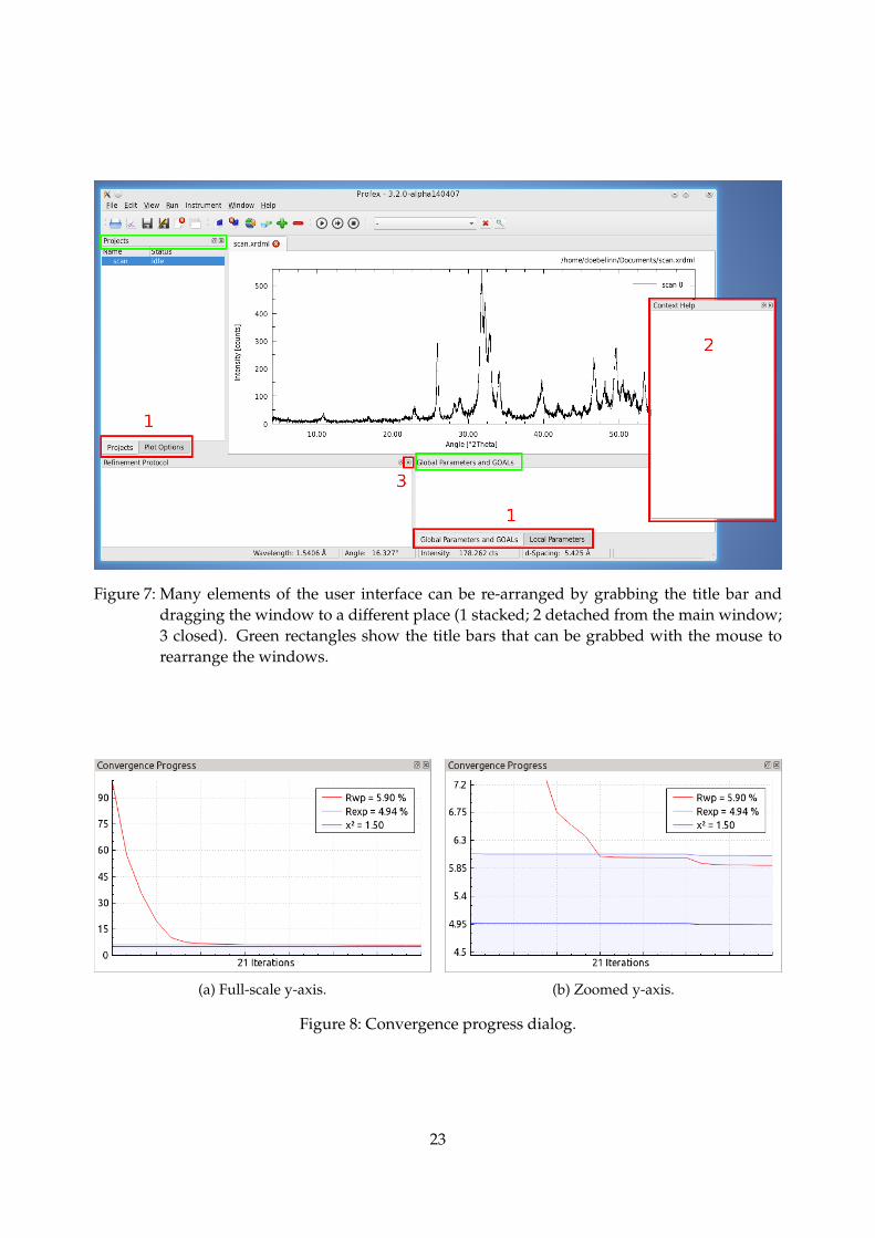
Figure 7: Many elements of the user interface can be re-arranged by grabbing the title bar anddragging the window to a different place (1 stacked; 2 detached from the main window;3 closed). Green rectangles show the title bars that can be grabbed with the mouse torearrange the windows.

(a) Full-scale y-axis. (b) Zoomed y-axis.

Figure 8: Convergence progress dialog.

23

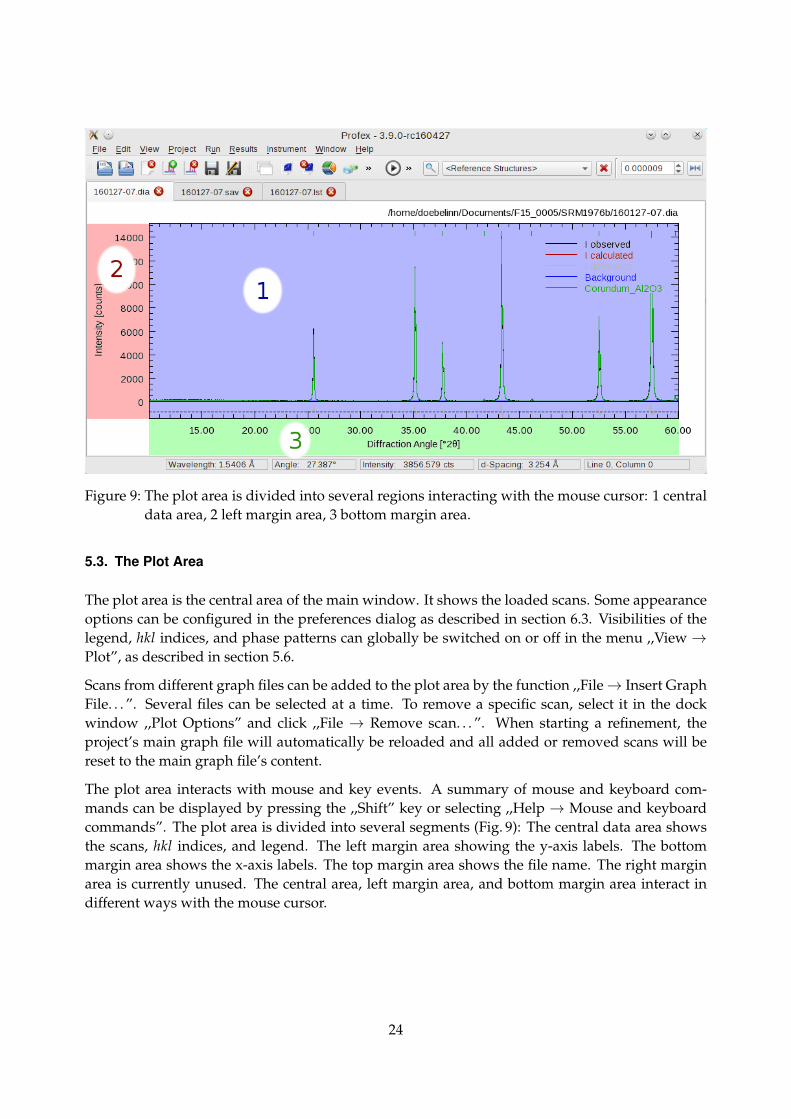
Figure 9: The plot area is divided into several regions interacting with the mouse cursor: 1 centraldata area, 2 left margin area, 3 bottom margin area.

5.3. The Plot Area

The plot area is the central area of the main window. It shows the loaded scans. Some appearanceoptions can be configured in the preferences dialog as described in section 6.3. Visibilities of thelegend, hkl indices, and phase patterns can globally be switched on or off in the menu ,,View→Plot”, as described in section 5.6.

Scans from different graph files can be added to the plot area by the function ,,File→ Insert GraphFile. . . ”. Several files can be selected at a time. To remove a specific scan, select it in the dockwindow ,,Plot Options” and click ,,File → Remove scan. . . ”. When starting a refinement, theproject’s main graph file will automatically be reloaded and all added or removed scans will bereset to the main graph file’s content.

The plot area interacts with mouse and key events. A summary of mouse and keyboard com-mands can be displayed by pressing the ,,Shift” key or selecting ,,Help → Mouse and keyboardcommands”. The plot area is divided into several segments (Fig. 9): The central data area showsthe scans, hkl indices, and legend. The left margin area showing the y-axis labels. The bottommargin area shows the x-axis labels. The top margin area shows the file name. The right marginarea is currently unused. The central area, left margin area, and bottom margin area interact indifferent ways with the mouse cursor.

24

5.3.1. Central Data Area

Moving the mouse cursor: The cursor position will be displayed in the status bar at the bottomof the main window. The horizontal and vertical position will be shown in degrees 2θ andcounts or counts per second, depending on the unit of the y-axis (see section 6). Addition-ally, the horizontal position will also be shown as d value in A. The wavelength is used tocalculate d values. If no wavelength information is found in the scan file, Profex will use thedefault wavelength specified in the preferences (see section 6).

Hovering the mouse pointer on a hkl index line at the top of the plot will show a tool tipdisplaying the phase name, hkl Miller indices, and the texture factor.

Left Mouse Button – Zooming: Use the left mouse button and drag the mouse to zoom into theplot.

Alternatively use the mouse scroll wheel to zoom horizontally to the location of the mousecursor, or hold the Ctrl key and use the scroll wheel to zoom vertically to the location of themouse cursor.

Hold the Ctrl key and left mouse button to move the zoomed scan.

Right Mouse Button – Unzooming: Click the right mouse button in the data area to view the en-tire scan range.

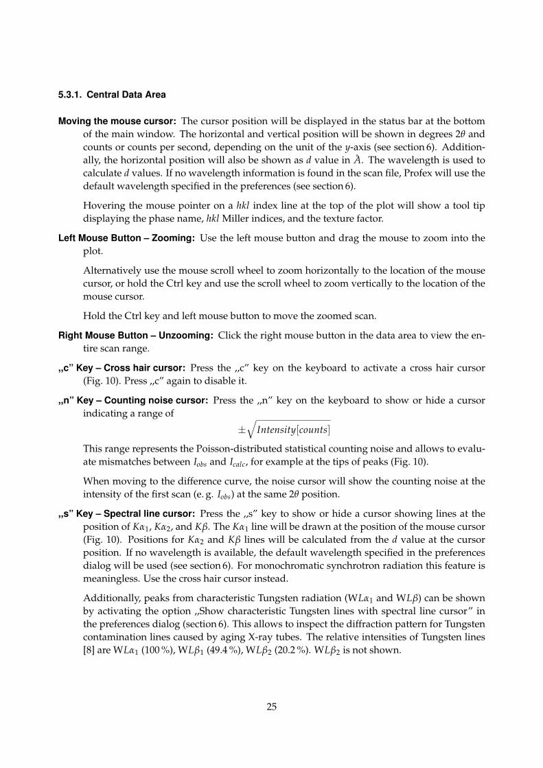
,,c” Key – Cross hair cursor: Press the ,,c” key on the keyboard to activate a cross hair cursor(Fig. 10). Press ,,c” again to disable it.

,,n” Key – Counting noise cursor: Press the ,,n” key on the keyboard to show or hide a cursorindicating a range of

±√

Intensity[counts]

This range represents the Poisson-distributed statistical counting noise and allows to evalu-ate mismatches between Iobs and Icalc, for example at the tips of peaks (Fig. 10).

When moving to the difference curve, the noise cursor will show the counting noise at theintensity of the first scan (e. g. Iobs) at the same 2θ position.

,,s” Key – Spectral line cursor: Press the ,,s” key to show or hide a cursor showing lines at theposition of Kα1, Kα2, and Kβ. The Kα1 line will be drawn at the position of the mouse cursor(Fig. 10). Positions for Kα2 and Kβ lines will be calculated from the d value at the cursorposition. If no wavelength is available, the default wavelength specified in the preferencesdialog will be used (see section 6). For monochromatic synchrotron radiation this feature ismeaningless. Use the cross hair cursor instead.

Additionally, peaks from characteristic Tungsten radiation (WLα1 and WLβ) can be shownby activating the option ,,Show characteristic Tungsten lines with spectral line cursor” inthe preferences dialog (section 6). This allows to inspect the diffraction pattern for Tungstencontamination lines caused by aging X-ray tubes. The relative intensities of Tungsten lines[8] are WLα1 (100 %), WLβ1 (49.4 %), WLβ2 (20.2 %). WLβ2 is not shown.

25

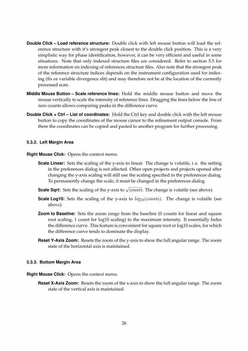
Double Click – Load reference structure: Double click with left mouse button will load the ref-erence structure with it’s strongest peak closest to the double click position. This is a verysimplistic way for phase identification, however, it can be very efficient and useful in somesituations. Note that only indexed structure files are considered. Refer to section 5.5 formore information on indexing of references structure files. Also note that the strongest peakof the reference structure indices depends on the instrument configuration used for index-ing (fix or variable divergence slit) and may therefore not be at the location of the currentlyprocessed scan.

Middle Mouse Button – Scale reference lines: Hold the middle mouse button and move themouse vertically to scale the intensity of reference lines. Dragging the lines below the line ofzero counts allows comparing peaks in the difference curve.

Double Click + Ctrl – List of coordinates: Hold the Ctrl key and double click with the left mousebutton to copy the coordinates of the mouse cursor to the refinement output console. Fromthere the coordinates can be copied and pasted to another program for further processing.

5.3.2. Left Margin Area

Right Mouse Click: Opens the context menu:

Scale Linear: Sets the scaling of the y-axis to linear. The change is volatile, i. e. the settingin the preferences dialog is not affected. Other open projects and projects opened afterchanging the y-axis scaling will still use the scaling specified in the preferences dialog.To permanently change the scale, it must be changed in the preferences dialog.

Scale Sqrt: Sets the scaling of the y-axis to√

counts. The change is volatile (see above).

Scale Log10: Sets the scaling of the y-axis to log10(counts). The change is volatile (seeabove).

Zoom to Baseline: Sets the zoom range from the baseline (0 counts for linear and squareroot scaling, 1 count for log10 scaling) to the maximum intensity. It essentially hidesthe difference curve. This feature is convenient for square root or log10 scales, for whichthe difference curve tends to dominate the display.

Reset Y-Axis Zoom: Resets the zoom of the y-axis to show the full angular range. The zoomstate of the horizontal axis is maintained.

5.3.3. Bottom Margin Area

Right Mouse Click: Opens the context menu:

Reset X-Axis Zoom: Resets the zoom of the x-axis to show the full angular range. The zoomstate of the vertical axis is maintained.

26

(a)

(b)

(c)

Figure 10: Different cursors of the plot area: (a) counting noise cursor, (b) cross hair cursor, (c)spectral lines cursor.

27

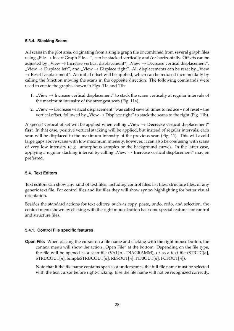
5.3.4. Stacking Scans

All scans in the plot area, originating from a single graph file or combined from several graph filesusing ,,File→ Insert Graph File. . . ”, can be stacked vertically and/or horizontally. Offsets can beadjusted by ,,View→ Increase vertical displacement”, ,,View→ Decrease vertical displacement”,,,View→ Displace left”, and ,,View→ Displace right”. All displacements can be reset by ,,View→ Reset Displacement”. An initial offset will be applied, which can be reduced incrementally bycalling the function moving the scans in the opposite direction. The following commands wereused to create the graphs shown in Figs. 11a and 11b:

1. ,,View→ Increase vertical displacement” to stack the scans vertically at regular intervals ofthe maximum intensity of the strongest scan (Fig. 11a).

2. ,,View→Decrease vertical displacement” was called several times to reduce – not reset – thevertical offset, followed by ,,View→ Displace right” to stack the scans to the right (Fig. 11b).

A special vertical offset will be applied when calling ,,View → Decrease vertical displacement”first. In that case, positive vertical stacking will be applied, but instead of regular intervals, eachscan will be displaced to the maximum intensity of the previous scan (Fig. 11). This will avoidlarge gaps above scans with low maximum intensity, however, it can also be confusing with scansof very low intensity (e. g. amorphous samples or the background curve). In the latter case,applying a regular stacking interval by calling ,,View→ Increase vertical displacement” may bepreferred.

5.4. Text Editors

Text editors can show any kind of text files, including control files, list files, structure files, or anygeneric text file. For control files and list files they will show syntax highlighting for better visualorientation.

Besides the standard actions for text editors, such as copy, paste, undo, redo, and selection, thecontext menu shown by clicking with the right mouse button has some special features for controland structure files.

5.4.1. Control File specific features

Open File: When placing the cursor on a file name and clicking with the right mouse button, thecontext menu will show the action ,,Open File” at the bottom. Depending on the file type,the file will be opened as a scan file (VAL[n], DIAGRAMM), or as a text file (STRUC[n],STRUCOUT[n], SimpleSTRUCOUT[n], RESOUT[n], PDBOUT[n], FCFOUT[n]).

Note that if the file name contains spaces or underscores, the full file name must be selectedwith the text cursor before right-clicking. Else the file name will not be recognized correctly.

28

(a)V

erti

cally

stac

ked

(b)V

erti

cally

and

hori

zont

ally

stac

ked

(c)R

egul

arof

fset

(d)A

dapt

ive

offs

et

Figu

re11

:Sta

cked

scan

s.

29

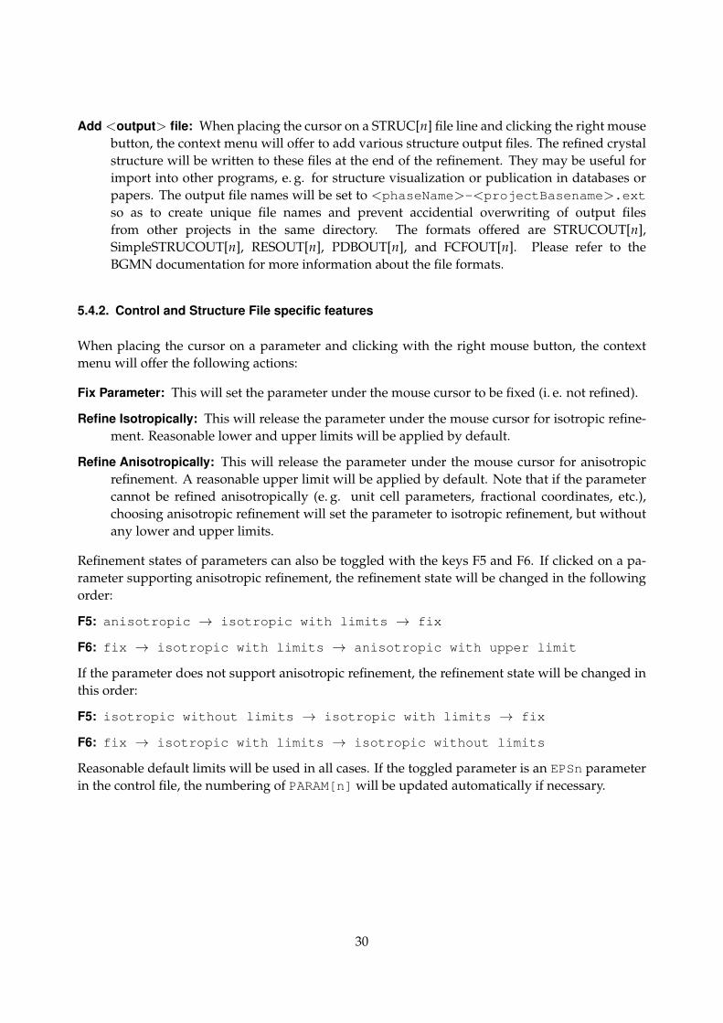
Add <output> file: When placing the cursor on a STRUC[n] file line and clicking the right mousebutton, the context menu will offer to add various structure output files. The refined crystalstructure will be written to these files at the end of the refinement. They may be useful forimport into other programs, e. g. for structure visualization or publication in databases orpapers. The output file names will be set to <phaseName>-<projectBasename>.extso as to create unique file names and prevent accidential overwriting of output filesfrom other projects in the same directory. The formats offered are STRUCOUT[n],SimpleSTRUCOUT[n], RESOUT[n], PDBOUT[n], and FCFOUT[n]. Please refer to theBGMN documentation for more information about the file formats.

5.4.2. Control and Structure File specific features

When placing the cursor on a parameter and clicking with the right mouse button, the contextmenu will offer the following actions:

Fix Parameter: This will set the parameter under the mouse cursor to be fixed (i. e. not refined).

Refine Isotropically: This will release the parameter under the mouse cursor for isotropic refine-ment. Reasonable lower and upper limits will be applied by default.

Refine Anisotropically: This will release the parameter under the mouse cursor for anisotropicrefinement. A reasonable upper limit will be applied by default. Note that if the parametercannot be refined anisotropically (e. g. unit cell parameters, fractional coordinates, etc.),choosing anisotropic refinement will set the parameter to isotropic refinement, but withoutany lower and upper limits.

Refinement states of parameters can also be toggled with the keys F5 and F6. If clicked on a pa-rameter supporting anisotropic refinement, the refinement state will be changed in the followingorder:

F5: anisotropic → isotropic with limits → fix

F6: fix → isotropic with limits → anisotropic with upper limit

If the parameter does not support anisotropic refinement, the refinement state will be changed inthis order:

F5: isotropic without limits → isotropic with limits → fix

F6: fix → isotropic with limits → isotropic without limits

Reasonable default limits will be used in all cases. If the toggled parameter is an EPSn parameterin the control file, the numbering of PARAM[n] will be updated automatically if necessary.

30

5.5. Tool bars

All functions shown in the main toolbar, project toolbar, and refinement toolbar are also accessiblein the menu bar and are described in detail in section 5.6. Toolbars can be re-arranged by draggingthe left end to another position, or shown / hiden by right-clicking on a toolbar and checking orunchecking the toolbar in the context menu.

Elements of the reference structure toolbar are only visible if at least one project is loaded. Theyare not accessible through a menu, only by the toolbar buttons:

Reference structures: A menu allowing to select a reference structure from all STR files foundin the structure database directory. If selected, the STR file’s hkl lines will be shown in thegraph. This is a generic way of phase identification. When using the ,,Add Phase” dialogwhile a reference structure is displayed, this structure file will be pre-selected in the ,,AddPhase” dialog.

If STR files have not been indexed before, hkl indices will be calculated on the fly when thestructure is selected. On modern computers, this only takes a second or two. Afterwardsthe hkl positions will be buffered and be available instantly. The buffer can be cleared asdescribed in section 6.6. Note that the double-click function described in section 5.3 is onlyavailable for indexed reference structures.

Reset reference structure: This button will reset the reference structure dropdown menu andhide reference hkl lines. After resetting, no structure will be pre-selected in the ,,Add Phase”dialog anymore.

Search and index new reference structures: Pressing this button will scan the structure databasedirectory for new STR files and index all new files. The reference structures become imme-diately available in all projects.

5.6. Menu Structure

5.6.1. File

Open Text File. . . (Ctrl+O) Opens a file in a text editor. If a project with the same name as thetext file’s base name is already open, the file is opened in this project. Else a new project iscreated.

If the text file is a control or results file, Profex will automatically locate all other control andresults files of the same project, as well as the scan file, and open them, too. Non-existingfiles are ignored.

BGMN structure files (*.str) are always opened in the currently shown project, regardless ofthe project name.

Open Graph File. . . (Ctrl+G) Opens a scan file in the graph page. If a control and/or results filewith the same base name is found, Profex will open it, too.

31

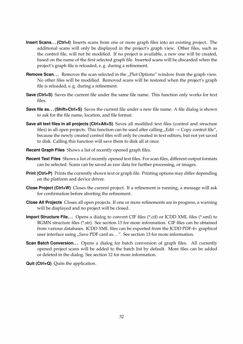
Insert Scans. . . (Ctrl+I) Inserts scans from one or more graph files into an existing project. Theadditional scans will only be displayed in the project’s graph view. Other files, such asthe control file, will not be modified. If no project is available, a new one will be created,based on the name of the first selected graph file. Inserted scans will be discarded when theproject’s graph file is reloaded, e. g. during a refinement.

Remove Scan. . . Removes the scan selected in the ,,Plot Options” window from the graph view.No other files will be modified. Removed scans will be restored when the project’s graphfile is reloaded, e. g. during a refinement.

Save (Ctrl+S) Saves the current file under the same file name. This function only works for textfiles.

Save file as. . . (Shift+Ctrl+S) Saves the current file under a new file name. A file dialog is shownto ask for the file name, location, and file format.

Save all text files in all projects (Ctrl+Alt+S) Saves all modified text files (control and structurefiles) in all open projects. This function can be used after calling ,,Edit→ Copy control file”,because the newly created control files will only be created in text editors, but not yet savedto disk. Calling this function will save them to disk all at once.

Recent Graph Files Shows a list of recently opened graph files.

Recent Text Files Shows a list of recently opened text files. For scan files, different output formatscan be selected. Scans can be saved as raw data for further processing, or images.

Print (Ctrl+P) Prints the currently shown text or graph file. Printing options may differ dependingon the platform and device driver.

Close Project (Ctrl+W) Closes the current project. If a refinement is running, a message will askfor confirmation before aborting the refinement.

Close All Projects Closes all open projects. If one or more refinements are in progress, a warningwill be displayed and no project will be closed.

Import Structure File. . . Opens a dialog to convert CIF files (*.cif) or ICDD XML files (*.xml) toBGMN structure files (*.str). See section 13 for more information. CIF files can be obtainedfrom various databases. ICDD XML files can be exported from the ICDD PDF-4+ graphicaluser interface using ,,Save PDF card as. . . ”. See section 13 for more information.

Scan Batch Conversion. . . Opens a dialog for batch conversion of graph files. All currentlyopened project scans will be added to the batch list by default. More files can be addedor deleted in the dialog. See section 12 for more information.

Quit (Ctrl+Q) Quits the application.

32

5.6.2. Edit

Undo (Ctrl+Z) Reverts the last change in the currently shown text file.

Redo (Shift+Ctrl+Z) Restores the last undone change in the currently shown text file.

Copy Control File Copies the current project’s control file to other projects and adapts all inputand output file names to match the projects’ base names. A dialog will allow to select whichprojects’ control file shall be modified. Existing control files will be overwritten.

Note that this function does not check whether referenced structure files are actually presentin all project directories. It only manages control files, but not structure files.

Insert Text Block Inserts the selected pre-defined text block to the current text editor at the cur-sor’s position. If a graph is shown, this action will do nothing. Text blocks can be configuredin the preferences dialog.

Reset File Reverts the current project’s control file to the state before the last refinement. Thisfunction is only used for the Fullprof.2k backend, but not for BGMN, because BGMN usuallydoes not modify STR and SAV files.

Find and Replace. . . (Ctrl+F) Searches a string in a control or structure file, and replaces it. If,,use Regular Expression” is checked, the ,,Find” keyword will be interpreted as a regularexpression pattern.

Preferences. . . Opens the program’s preferences dialog. All preference options are discussed indetail in section 6.

5.6.3. View

Switch to Graphs (Ctrl+1) Raises the Graph page of all projects.

Switch to Control Files (Ctrl+2) Raises page 2 (usually the control file) of all projects.

Switch to Output Files (Ctrl+3) Raises page 3 (usually the results file) of all projects.

Set Zoom Range. . . Opens a dialog to zoom the graph to precise upper and lower limits for angleand intensity.

Reset margin color Resets the color of the graph margin to idle color. This is useful for takingscreenshots after completed refinements.

Show/Hide Phase Patterns (Ctrl+0) Activates or deactivates visibility of all phases. This optionapplies to all open projects. It only checks or unchecks the visibility boxes of all phase pat-terns in the Plot Options list for convenient displaying or hiding of all phases. Individualphases can be shown or hidden by selecting or un-selecting the ,,show” option in the PlotOptions list. More information is given in section 5.2.2.

Plot Configure the visibility of the following elements on the plot:

Phase Patterns Shows or hides patterns of phases.

33

Legend Shows or hides the plot legend.

hkl Indices Shows or hides the hkl index tick marks at the top of the plots.

Increase Vertical Displacement (Ctrl+Up) Applies a regular vertical offset to all scans. The initialoffset will correspond to the maximum intensity of the strongest scan. When called again,this function will increase the previous offset by a constant value.

Decrease Vertical Displacement (Ctrl+Down) Reduces the vertical offset of all scans by a constantvalue. If no vertical offset exists, an initial adaptive offset will be applied, with a verticaldisplacement of each scan corresponding to the maximum intensity of the scan below.

Displace left (Ctrl+Left) If no horizontal offset exists, it will apply a horizontal offset to the left toall scans. If an offset to the left exists, the offset will be increased by a constant value. If anoffset to the right exists, the offset will be reduced by a constant value.

Displace right (Ctrl+Right) If no horizontal offset exists, it will apply a horizontal offset to theright to all scans. If an offset to the right exists, the offset will be increased by a constantvalue. If an offset to the left exists, the offset will be reduced by a constant value.

Reset Displacement (Ctrl+Space) Resets all horizontal and vertical offsets.

5.6.4. Project

Add / Remove Phase. . . (F8) Opens a dialog to create or manage a control file. New phases canbe added or existing phases can be removed from the refinement. If no control file existsyet, a new one will be created. In that case, the correct instrument configuration file must beselected. The option to create a default control file is automatically activated or deactivated,depending on whether or not a control file already exists.

If a phase is activated in the Reference Phase box, it will be pre-selected in the Add Phaselist.

If a default control file is created despite an existing control file, the existing one will beoverwritten, any previously added modifications or phases will be lost.

Selected structure files and instrument configuration files will be copied from the structureand device database directory to the project directory. Files already existing in the destina-tion directory will be skipped. If the option ,,overwrite existing files” is checked, existingstructure files will be overwritten with the file copied from the structure file database. Seesection 7 for more information.

When removing a phase from the control file, the structure file can optionally be deleted.Deleting structure files may cause problems with other projects stored in the same directoryand accessing the same structure files.

Open all project STR files (Ctrl+F8) Opens all BGMN structure files (*.str) referenced in the cur-rent project’s control file (*.sav) in new pages.

34

Close all project STR files (Ctrl+F7) Closes all BGMN structure files (*.str) shown in the currentproject.

Set Internal Standard Allows to define one refined phase as internal standard phase with a givenquantity. The calculation of phase quantities will be changed to apply the internal standardcorrection, and the standard phase will no longer be shown in the summary table.

Unset Internal Standard Reverts the internal standard calculation of refined phase quantities. Allphases will be shown in the summary table in quantities normalized to the sum of all phases.

Refinement Presets Lists all refinement presets to create refinement control files. Select one ofthem to apply the preset to the current project. See section 7.2 for more information onrefinement presets.

Save as Refinement Preset. . . Creates a new refinement preset from the currently loaded project.See section 7.2 for more information on refinement presets.

Save Project Backup (Ctrl+B) Creates a ZIP compressed archive of the current project. The filename is determined automatically as projectBasename-YYYYMMDD-hhmm.zip. It willbe stored inside the current project’s working directory. The archive includes the raw datafile, all instrument files, structure files, and output files of the project.

Save Project Backup As. . . (Ctrl+Shift+B) Creates a ZIP compressed archive of the currentproject. The file name and path can be selected by the user. The archive includes theraw data file, all instrument files, structure files, and output files of the project. The ZIParchives can be stored as a backup or shared with other users, as they contain all projectrelevant data.

5.6.5. Run

Run Refinement (F9) Starts the refinement of the currently shown project.

Run Batch Refinement (F10) Starts a batch refinement of all open projects.

Abort Current Refinement (Ctrl+C) Aborts refinement of the currently shown project. In batchrefinement mode all projects scheduled for batch refinement will be unscheduled. If the cur-rently shown project is not running but scheduled, it will be unscheduled but the remainingbatch refinement will not be interrupted. In either case refinements started outside of thebatch will not be interrupted.

Abort All Refinemet (Shift+Ctrl+C) Aborts all running projects and batches. If more projects thanthe currently shown one are affected, the user will be asked for confirmation.

Follow Active Refinement When processing a batch refinement, activate this function to alwaysraise the currently refining project. If a project refinement has completed, the next scheduledproject will automatically be raised. This allows to monitor the batch refinement on screen.The function can be toggled on and off at any time, also during a running batch. It is au-tomatically deactivated as soon as the user selects a text editor of any open project, so as toavoid automatically raising a different project while a text file is being edited or read.

35

5.6.6. Results

Export Global Parameters and GOALs (Ctrl+E) Exports the global parameters and goals (e. g.phase quantities) to a semicolon separated spread sheet (*.csv). See section 8.3.1 for moreinformation.

Export Local Parameters and GOALs (Shift+Ctrl+E) Exports the local parameters and goals (e. g.structural parameters) to a semicolon separated spread sheet (*.csv). See section 8.3.1 formore information.

Export Chemistry. . . Writes the calculated chemical composition to a semicolon separated spreadsheet (*.csv). See section 8.3.1 for more information.

Export CIF file from LST file This function reads LST files of all open projects and writes crystalstructure information to CIF files. One CIF file will be created for each crystal structurefound. The file will be stored in the project directory. Information on saved files is shown inthe refinement protocol console.

Export CELL file from RES file This function reads RES files of all open projects and writes crystalstructure information to CELL files for the software Castep [9]. One CELL file will be createdfor each crystal structure found. The file will be stored in the project directory. Informationon saved files is shown in the refinement protocol console. If no RES file is available for aspecific phase, a tag RESOUT[n]=filename.res must be added to the control file (*.sav)and the refinement must be repeated.

5.6.7. Instrument

New Configuration. . . Read some hardware information from Bruker RAW V4, Bruker BRML V5,and PANalytical XRDML files to create a BGMN instrument configuration file from scratch.Other raw data formats are not supported. Usually several variable required by BGMN willstill not be available from the raw data files and will thus have to be entered manually. Seesection 14 for more information.

Edit Configuration. . . Opens a dialog to process BGMN instrument configurations. See section14 for more information.

Learn Profile. . . Opens a dialog to process BGMN instrument configurations using the ,,LearntProfile” approach.

Show Peak Shape. . . Opens a dialog that calculates the theoretical peak shapes for a selectedinstrument configuration file.

36

5.6.8. Window

Projects Shows or hides the Projects list window.

Plot Options Shows or hides the Plot Options window.

Refinement Protocol Shows or hides the Refinement Protocol window.

Global Parameters and GOALs Shows or hides the summary table window for global parametersand goals.

Local Parameters Shows or hides the summary table window for local parameters and goals.

Chemistry Shows or hides the table showing the refined chemical composition in oxide form.

Context Help Shows or hides the context help display.

Convergence Progress Shows or hides the window showing a graph with Rwp and Rexp valuesduring a refinement.

5.6.9. Help

Context Help. . . (F1) Shows the context help of the keyword under the text cursor. The ,,ContextHelp” window (,,View” menu) must be shown to display the context help.

BGMN Variables. . . Opens a web browser showing the BGMN variables documentation page.

BGMN SPACEGRP.DAT. . . Opens a dialog to browse spacegroups and atomic positions sup-ported by BGMN.

BGMN Atomic Scattering Factors. . . Opens a dialog to browse atomic scattering (form) factorssupported by BGMN. The dialog reads the file AFAPARM.DAT, which is part of the BGMNsoftware distribution.

Mouse and Keyboard Commands Shows a dialog with mouse and keyboard commands for plotwindows.

About Profex. . . Shows information about Profex.

37

6. Preferences

6.1. General

Toolbar Layout Select how icons and text in Profex’ toolbars are shown. ,,Follow Style” will matchthe system-wide style used by the operating system.

Restore open projects If checked, Profex will load all previously open graph files upon programstart. If unchecked, Profex will not load any projects or files at program start.

Default Project Type For file formats not specific for either BGMN or Fullprof.2k, this option de-termines which type of project will be created when such a file is opened. The file type isidentified by the file extension.

File extensions can also be associated with either of the two backends by adding the ex-tension either to the list of ,,File Extensions associated with BGMN” or ,,File Extensionsassociated with Fullprof”.

Number of CPU cores used by BGMN Specifies how many CPU cores will be used by the refine-ment backend (only available for BGMN). ,,Automatic” will use all available cores.

File Extensions associated with Fullprof These file types will always be opened as Fullprofprojects, regardless of the default project type. Enter the extension in small letters withoutasterisks and periods, separated by a space character. Example: pcr dat sum prf

File Extensions associated with BGMN These file types will always be opened as BGMNprojects, regardless of the default project type. Enter the extension in small letters withoutasterisks and periods, separated by a space character. Example: sav lst dia str

Default Wavelength This wavelength, given in A, is used for scan files not containing any infor-mation about the wavelength.

Always use default Wavelength If checked, Profex will ignore the wavelength read from the scanfile and always use the default wavelength to calculate d values from diffraction angles. Usethis option with care. Any wavelength information read from raw data files will be ignoredif this option is checked.

6.2. Text Editors

Font Sets the font of the text editor and refinement protocol window.

38

6.3. Graphs

Use AntiAliasing for Graphs (slow!) Uses anti aliasing to draw the plots. If checked, lines looksmoother but also wider. Drawing will be slower if checked.

Show characteristic Tungsten lines with spectral line cursor When using the spectral line cursor(5.3), additional lines will be shown for characteristic Tungsten radiation (WLα1 and WLβ1).This allows to inspect the diffraction pattern for Tungsten contamination lines caused byaging X-ray tubes.

Show major grid lines Show or hide vertical and horizontal grid lines at the positions of majortick marks. Major grid lines will be drawn as medium dashed lines.

Show minor grid lines Show or hide vertical and horizontal grid lines at the positions of minortick marks. Minor grid lines will be drawn as light dotted lines.

Display Line Width Width in pixels of all lines (plots, axes, tick marks) of the graph on computerscreens. If plot lines are too fine (e. g. on high-resolution displays) increase this value.

Printing Line Width Width in points of all lines (plots, axes, tick marks) of the graph on printouts.This value should usually be greater than the display line width. It has to be matched to theprinter device driver by printing test plots.

Symbol Size Size of the measured data points when not using solid lines (e. g. dots or crosses) inpixels.

Y-axis Scaling Scaling of the y-axis. Options are linear, logarithmic with a base of 10 (log10), orsquare root (sqrt).

Y-axis unit Shows the y-axis unit either in counts, or in counts per second (cps). Counts persecond may not be available, depending on the file format of the loaded scan. If the time perstep is not available, Profex will fall back to the unit ,,Counts” and assume a counting timeof 1 second per step.

Only the display of scans will be affected by the choice of the unit. Internally, all calcula-tions and file format conversions will be performed in ,,Counts”. As a consequence, whenconverting a format supporting ,,Counts per second” (such as XRDML) to a format not sup-porting it (such as ASCII XY), the displayed unit may change from [cps] to [counts].

Multi-Scan Files Select whether multi-range files will be shown as individual scans, as the sumof all ranges, or as the average of all ranges.

Create Thumbnail If checked, a thumbnail picture of the refined plot will be created atthe end of the refinement. This file is stored in the project directory with the nameproject-basename tn.png. It allows easy browsing of refined projects. The widthof the picture can be specified in pixels. The height is calculated from the displayed aspectratio.

Background color idle Select the color of the graph’s margin in idle state. Usually white is thepreferred option.

39

Background color active Select the color of the graph’s margin in active state (during refine-ments). The default is light red. If no color change is preferred, select the same color asfor idle state.

Background color complete Select the color of the graph’s margin in complete state (after con-vergence of refinements). The default is light green. If no color change is preferred, selectthe same color as for idle state. The margin color can be set back to idle color by clicking,,View→ Reset margin color”.

6.3.1. Fonts

Font Title Select the font of the file name at the top-right of the graph.

Font Axis Labels Select the font of the graph axis labels.

Font Tick Marks Select the font of the graph tick marks.

Font Legend Select the font of the graph legend.

6.3.2. Scan Styles

Color Customize the list of colors to be used to draw scans by double-clicking on the color cell. Ifmore scans are loaded than colors are available from the list, a random color will be createdand added to the list. It can be changed manually later. Line widths can be changed on theGraph’s General Appearance page.

Point Style Select the style to draw scans. ,,Solid” draws the scan as a solid line. ,,Points” draws adot at the measured position, ,,Cross” draws a cross at the measured position. Symbol sizesof crosses and points can be changed on the Graph’s General Appearance page.

+ Add another color to the color list.

− Remove the currently selected color from the list.

6.4. BGMN

BGMN Executable Selects the BGMN executable file. This file is part of the BGMN installation. Itis called BGMN.EXE on Windows, and bgmn on Mac OS X and Linux.

MakeGEQ Executable Selects the MakeGEQ executable file. This file is part of the BGMN instal-lation. It is called MakeGEQ.EXE on Windows, and makegeq on Mac OS X and Linux.

Geomet Executable Selects the Geomet executable file. This file is part of the BGMN installation.It is called GEOMET.EXE on Windows, and geomet on Mac OS X and Linux.

Output Executable Selects the Output executable file. This file is part of the BGMN installation.It is called OUTPUT.EXE on Windows, and output on Mac OS X and Linux.

40

Verzerr Executable Selects the Verzerr executable file. This file is part of the BGMN installation.It is called VERZERR.EXE on Windows, and verzerr on Mac OS X and Linux.

Gertest Executable Selects the Gertest executable file. This file is part of the BGMN installation.It is called GERTEST.EXE on Windows, and gertest on Mac OS X and Linux.

Run in WINE This box is only available on Linux and Mac OS X. It allows to use the Windowsversion of BGMN to be run in WINE. Check this option if the executable files specifiedabove belong to the Windows version of BGMN.

Structure Files Directory Specifies the location where BGMN structure files (*.str) are stored. Sev-eral directories can be entered. Sub-directories will be scanned for *.str files, too. This allowsto use a shared network structure repository and a local personal one simultaneously.

Device Files Directory Specifies the location where BGMN instrument files (*.sav, *.ger, *.geq,*.tpl) are stored.

Presets Directory Specifies the location where refinement preset files (*.pfp) are stored. See sec-tion 7.2 for more information on presets.

Convert raw scans to XY format If checked, raw scan files will be converted to ASCII XY freeformat (*.xy) prior to starting the refinement.

This option must only be disabled if the raw file format is directly supported by the BGMNbackend (e. g. *.val, *.rd).

Manage phase quantification GOALs If this option is checked, a GOAL to compute relative phasequantities will be added automatically if a new phase is added from the ,,Add / RemovePhase” dialog. Example: Adding a new structure ,,vaterite.str” to a control file with thefollowing phase content:

STRUC[1]=calcite.strSTRUC[2]=aragonite.str...sum=calcite+aragoniteGOAL[1]=calcite/sumGOAL[2]=aragonite/sum

If this option is checked, the control file will be modified as follows:

STRUC[1]=calcite.strSTRUC[2]=aragonite.strSTRUC[3]=vaterite.str...sum=calcite+aragonite+vateriteGOAL[1]=calcite/sumGOAL[2]=aragonite/sumGOAL[3]=vaterite/sum

41

The GOAL section will be completely rewritten each time a phase is added or removed. Anycustomizations will be overwritten.

If this option is not checked, the file will be modified as follows:

STRUC[1]=calcite.strSTRUC[2]=aragonite.strSTRUC[3]=vaterite.str...sum=calcite+aragoniteGOAL[1]=calcite/sumGOAL[2]=aragonite/sum

Note that in the second case, no GOALs will be modified. Any customizations will be pre-served, but the GOAL computation for the newly added or removed phase must be updatedmanually.

Spectral line cursor shows all wavelengths from BGMN *.lam file By default Profex uses a hard-coded table of characteristic wavelengths to display the spectral lines of Kα1, Kα2, and Kβ

with the spectral line cursor. The primary wavelength is read from the scan file (raw data fileor refined profile), and all related secondary wavelengths are found in the hard-coded table.If this option is checked, Profex will try to locate the *.lam file specified in the BGMN refine-ment control file using the keyword LAMBDA=, and read all wavelengths specified there.

The radiation spectrum in the *.lam file is often modeled by overlapping Lorentzian curves.It is therefore not unusual to use 4 or more emission lines with slightly different wavelength,widths, and intensities to model Kα1 and Kα2 with realistic emission line profiles. If addition-ally Kα3 satellites and Kβ are modeled, even more emission lines are required. The emissionspectrum described in the *.lam file can therefore be relatively complex, and displaying alllines with the spectral line cursor can lead to a cluttered plot display. For most users usingconventional X-ray tubes with characteristic radiation spectra, with or without Kβ filters ormonochromators, leaving this option unchecked is recommended.

If the *.lam file was not specified, cannot be found, or cannot be parsed, Profex falls backto the internal hard-coded table of characteristic wavelengths, just as if this option wasunchecked.

Any comment trailing the emission line parameters will be used to label the line. For exam-ple, to add line labels to the file ,,cu bergmann83.lam”, which is part of the Profex-BGMN-Bundle distribution:

% Cu-K-alpha doublet as measured in october 1983 by J. BergmannILAM=4 TITEL=CU_vom_Oktober_19830.401939 6.49098 0.00109810.266445 6.49013 0.00198750.167844 6.47504 0.00125440.163773 6.47400 0.0017246

42

add comments to each data line:

% Cu-K-alpha doublet as measured in october 1983 by J. BergmannILAM=4 TITEL=CU_vom_Oktober_19830.401939 6.49098 0.0010981 % CuKa1 (1)0.266445 6.49013 0.0019875 % CuKa1 (2)0.167844 6.47504 0.0012544 % CuKa2 (1)0.163773 6.47400 0.0017246 % CuKa2 (2)

Now the emission lines will be labelled as ,,CuKa1 (1)”, ,,CuKa1 (2)” etc. when activatingthe spectral line cursor. *.lam files with parametrized intensities are also supported, as forexample the default ,,cu.lam” file distributed with the Profex-BGMN-Bundle package:

% Berger CuK1,2,3 + Kb XPERT BERNILAM=60.01586*ifthenelse(ifdef(alpha3ratio),(alpha3ratio)/0.01586,1) 6.51571 0.00783 % CaKa30.56768*ifthenelse(ifdef(alpha2ratio),(1-alpha2ratio)/0.64369,1) 6.49099 0.00092 % CuKa1 (1)0.07601*ifthenelse(ifdef(alpha2ratio),(1-alpha2ratio)/0.64369,1) 6.48905 0.00126 % CuKa1 (2)0.25107*ifthenelse(ifdef(alpha2ratio),(alpha2ratio)/0.35631,1) 6.47496 0.00109 % CuKa2 (1)0.08688*ifthenelse(ifdef(alpha2ratio),(alpha2ratio)/0.35631,1) 6.47366 0.00130 % CuKa2 (2)0.00249*ifthenelse(ifdef(betaratio),(betaratio)/0.00249,1) 7.18206 0.00151 % CuKb

6.4.1. Structure File Handling

Custom Profile Function

Use custom profile function Check this option if Profex should automatically change the profileparameters of BGMN Structure files (*.str). The files will be modified when they are copiedfrom the structure database to the project directory by calling ,,Edit→ Add Phase. . . ”. If thisoption is disabled, the profile parameters will not be changed.

Profile Function (RP) Specify the RP=n parameter.

Scaling (GEWICHT) Specify the GEWICHT parameter. Choose SPHARn for refinement of preferredorientation, or ISOTROPIC for untextured samples.

Lorenzian Size Broadening (B1) Specify B1, enter ANISO for anisotropic crystallite sizes. Check,,refine” to refine this parameter.

Gaussian Size Broadening (k1) Specify k1. Check ,,refine” to refine this parameter.

Micro Strain (k2) Specify k2, enter ANISO4 for anisotropic micro-strain. Check ,,refine” to refinethis parameter.

GOALs

Add Default Goals Check this option if a set of default goals is to be added to each copied BGMNStructure file (*.str). Specify the goals in the text field below. Example:GrainSize(1,1,1) //

43

Micro-Absorption Correction

Add Correction for Micro-Absorption Check this option if a correction for micro-absorption(Brindley correction) shall be added to each copied structure file.

Default Function If checked, the correction formula is hard coded to a default function.

Custom Function Check this line and enter a custom correction function if a correction formulaother than the default one shall be used.

6.4.2. Limits

Unit Cell Parameters Specifies the range for upper and lower limits of unit cell parameters to beadded automatically to BGMN Structure files (*.str) created from CIF or ICDD XML structurefiles. The same limits will be applied if unit cell parameters are released for refinement inthe control file.

Fractional Coordinates Upper and lower limits are added to fractional coordinates released forrefinement. The unit of this value is in fractional coordinates. Example: Releasing the coor-dinates of the following atom for refinement with a limit of 0.05:

E=SI Wyckoff=f x=0.25 y=0.5 z=0.1234 TDS=0.02

will result in (without line break):

E=SI Wyckoff=f PARAM=x=0.25_0.20ˆ0.30 PARAM=y=0.5_0.45ˆ0.55PARAM=z=0.1234_0.0734ˆ0.1734 TDS=0.02

6.4.3. Summary Table

Global Parameters and GOALs

Show warnings for values below detection and quantification limit If activated, Profex willshow a warning for phase quantities getting small relative to their ESD. For example, ifthe limit of quantification (LOQ) is defined as 0.25, the relative standard deviation ESD /value must be smaller than 25 %, or, in other words, the refined value must be greater than4 · its ESD. Else a warning ,,¡ LOQ” will be shown in the summary table. See section 10 formore information.

Limit of quantification (LOQ): ESD / Value = Defines the threshold for ,,< LOQ” (below limit ofquantification) warnings. Typical values are 0.25 if the refined value must be at least fourtimes its ESD in order to be quantifiable, or 0.10 if it must be at least 10 times greater than itsESD. This variable can also be set in the control file (*.sav), see section 11. Values read fromthe control file override values specifiec in the preferences dialog. See section 10 for moreinformation.

44

Limit of detection (LOD): ESD / Value = Defines the threshold for ,,< LOD” (below limit of detec-tion) warnings. Typical values are 0.50 if the refined value must be at least twice its ESDin order to be detectable, or 0.33 if it must be at least three times greater than its ESD. Thisvariable can also be set in the control file (*.sav), see section 11. Values read from the controlfile override values specifiec in the preferences dialog. See section 10 for more information.

Minimum ESD (ignore ESDs below) = For phase quantities approaching 0.0, the ESD also ap-proaches 0.0. Such phases appear to be detectable and quantifiable even at infintesimallysmall quantities, but in fact it is an artifact of the ESD computation. In order to avoid this,a minimum ESD can be specified here. Refined ESDs below this value will be ignored andhard set to the minimum ESD. Typical values are 0.05 wt-%. Set this value to 0.00 to use allrefined ESD values, regardless of how small they are. See section 10 for more information.

Listed GOALs A list of global GOAL names that will be read from the BGMN list file (*.lst) andshown in the summary table for global parameters and goals. If the text field is empty,all global GOALs will be shown. This text field supports regular expression patterns. Forexample, instead of listing all EPSn values separately:

EPS1EPS2EPS3EPS4

one can use a regular expression to list all refined EPS values:

ˆEPS[1-4]$

or alternatively:

ˆEPS\d$

Regular expressions are useful to identify GOALs describing a phase quantity. QuantityGOALs managed by Profex always have a unique name ending on /sum. A regular expres-sion pattern describing GOAL names of type <any name>/sum can thus be used to list onlyphase quantity GOALs. The following pattern only matches GOALs with names ending on/sum:

ˆ[ˆ\/]+\/sum$

Numerous tutorials on regular expressions can be found on the internet.

Reset Pressing this button erases the text field with global parameters and GOALs and inserts adefault set of parameters.

45

Local Parameters and GOALs

Listed GOALs Enter the parameters to be read from the local parameters and goals section in theBGMN list file (*.lst) and shown in the summary table for local parameters and goals. Thetext field supports regular expression patterns. For example, instead of listing all unit cellparameters separately:

ABCALPHABETAGAMMA

one could use a regular expression patter

ˆA|B|C|ALPHA|BETA|GAMMA$

or alternatively:

ˆ[A-C]$ˆALPHA|BETA|GAMMA$

However, with regular expression patterns the parameters may be listed in arbitrary order.Regular expressions are particularly useful for GrainSize results. Printing all refined Grain-Sizes is achieved by the following pattern:

ˆGrainSize\(\d,\d,\d\)$

Reset Pressing this button erases the text field with local parameters and GOALs and inserts adefault set of parameters.

6.5. Fullprof

Fullprof Executable Specifies the path to the Fullprof executable fp2k.exe.

Structure files directory Specifies the location of the directory with structure template files.

Device files directory Specifies the location of the directory with device template files.

Stop on convergence Normally Fullprof aborts the refinement when convergence criteria arereached. Checking this option forces Fullprof to always perform the number of refinementcycles specified with the parameter Ncy.

Divergence slit angle As Fullprof expects all scans to be measured with a fixed divergence slitsetting, Profex will attempt to convert scans measured with automatic or variable divergenceslit. The slit opening in degreees specified here is the opening the scans will be converted to.A value less than 1.0 degree is recommended.

46

6.6. Reference Structures

Automatically select best matching reference phase When opening a graph file, automaticallysearch and select the reference phase with it’s strongest peak at the position of the scan’shighest intensity. This is the same as double clicking at the strongest peak just after loadingthe scan file. Note that only indexed reference structures will be considered.

Automatically index new structure files If checked, Profex will scan the structure file directoryfor new structure files each time Profex is started and the first project is loaded.

If not checked, new structures will be indexed the first time they are selected in the ReferenceStructures box.

Structures will not be available for double-click phase identification as long as they have notbeen indexed.

Color of Reference hkl Lines Color of the hkl lines when selecting a reference structure from theReference Structures box.

Clear hkl index buffer Clears the buffer file with structure file hkl indices. Profex must berestarted for this to take effect. All structure files will be re-indexed either automatically,or when selected from the Reference Structures box.

hkl reference line range Specifies the lower and upper 2θ angle for hkl indices to be calculated.Larger ranges will require more time to index. The range may be smaller or larger than scanfile ranges.

6.7. Chemical Composition

The chemical composition page allows to edit the oxide forms and their molecular weights usedto calculate the elemental composition of the sample. Elements with empty molecular weight,or with molecular weight of 0.0 g/mol, will be ignored. It is recommended to leave the oxideand molecular weight cells of oxygen (element No. 8) empty to suppress display of oxygen as aseparate element in the chemistry results table.

A dialog to select the oxide form and automatically calculate the corresponding molecular weightcan be opened by double-clicking on the element symbol (left column).

Double-clicking an oxide cell (middle column) or molecular weight cell (right column) allows toenter oxide names and molecular weights directly by bypassing the dialog mentioned above.

Element, Oxide, and Molecular Weight table This table holds the oxide formula and oxide molec-ular weight for each element. Edit the values by double clicking a cell. Double clicking anelement cell will open a dialog to determine oxides and their molecular weight. Doubleclicking any other cell allows direct input of oxide formulas and values.

Reset Resets the table to the internal default values. All customizations will be lost.

47

6.8. Text Blocks

Text blocks are pre-defined sections of text that needs to be inserted in control or structure filesregularly. Instead of entering the text manually each time, a text block can be selected from themenu and inserted conveniently at the mouse cursor position in the currently shown text editor.Click the + button to create a new text block, then enter the text in the editor. All changes will besaved automatically when closing the preferences dialog. Click − to delete the current text block.The block will be deleted permanently when closing the preferences dialog with the ,,OK” button.Close the dialog with ,,Abort” if the text block was deleted accidentally.

A common scenario for text blocks is the structure file code to activate sub-phase refinement. Thesame code is needed occasionally in structure files. It can thus be pre-defined in the preferencesand applied from the menu ,,Edit → Insert Text Blocks”. An example of the code is shown be-low.

RefMult=2

PARAM=pG=0.5_0ˆ1GEWICHT[1]=pG*GEWICHTGEWICHT[2]=(1-pG)*GEWICHT

PARAM=pB1=1_0.1ˆ10B1[1]=B1B1[2]=pB1*B1

48

7. Adding and Removing Structure Files

One of Profex’ central components is the ,,Add / Remove Phase” dialog (Fig. 12). It is accessedby clicking ,,Project→ Add / Remove Phase. . . ”, or pressing F8 or the corresponding button onthe project tool bar. This dialog is used to easily create or modify the refinement control file.It will automatically add a STRUC[n] reference and related GOALs for phase quantification tothe control file, and copy the selected STR files from the structure file database to the workingdirectory (Fig. 5). The individual elements of this dialog are described in detail below.

Generate default control file: If this option is checked, Profex will generate a default control filefor the selected instrument configuration. If a template file is found (section 3.4), it will beused to create the control file. Else Profex will present a dialog asking for basic informationabout the instrument configuration. If the option is active, an existing control file will beoverwritten. The default state of this option depends on the presence of a previous controlfile:

• If a control file was found, this function will be unchecked. Manually activating theoption will overwrite the existing control file with a newly created default file.

• If no control file was found, this function will be active.

Instrument configurations: This dropdown menu lists all instrument configurations found in thedevice database directory (section 3.4).

Structures: This list shows all structure files found in the structure file database directories (sec-tion 3.4). Files stored in a sub-directory will be shown in a tree structure that can be collapsedor expanded. Clicking on the header of the table (,,File Name”, ,,Phase”, or ,,Comment”) willsort the table in ascending or descending order of the clicked column. Structures selectedin the first column will be added to the control file. If a reference structure is shown on themain graph, it will be pre-selected in this dialog.

Expand/Collapse: If structure files are organized in sub-directories in the structure database di-rectory, they will be organized in a tree structure in this dialog. Clicking ,,Expand/Collapse”will expand or collapse all items in the tree structure for easy navigation.

Overwrite existing files: If a selected structure file is already present in the project directory, itwill normally not be overwritten. This preserves customized files. Checking this option willforce overwriting of existing files. Use this option with care, as other projects accessing thesame structure files will be affected, too.

Remove Phases: The phases listed here are currently referenced in the control file. Check theones that shall be removed from the refinement.

Delete Files: If this option is checked, the removed file will also be deleted from the hard diskin the project directory. This may cause problems with other projects residing in the samedirectory and referencing the same structure file. It is recommended to use this option withcare.

49

If the control file contains multiple references to the same structure file, only the first occur-rence will be removed. In that case, the option ,,Delete STR Files” will be ignored until thelast reference to this file was removed from the control file.

Note that only copies of structure files in the local project directory will be deleted. Thestructure file database directory will remain unchanged.

The ,,Add / Remove Phase” dialog will not allow to add the same phase more than once to acontrol file. If a selected file is already referenced in the control file, it will just be skipped by thedialog. If multiple entries of the same structure file are requested, the control file will have to bemodified by hand.

Figure 12: The ,,Add / Remove Phase” dialog showing all instrument configuration files (top),structure files found in the database directories, and structure files currently referencedin the control file.

7.1. Project organization

When working with several datasets (= projects) at a time, it is important to understand how Pro-fex’ ,,Add / Remove Phase” function handles structure and instrument files in the background.

By default the ,,Add / Remove Phase” dialog will copy selected structure and instrument files tothe location of the currently loaded scan file as shown in Fig. 12. It will check whether a file withthe same name is already present. If yes, the present file will not be overwritten, unless the option,,overwrite existing files” was activated for structure files, and ,,generate default control file” wasactivated manually for instrument files.

50

Since several raw scan files can be located in the same directory, a structure file will only be presentonce, even if it was added multiple times for each project. Modifying, removing, or overwritingthis structure file will affect all projects within this directory (Fig. 13).

If common structure files are not desired, there are several options to avoid shared access bymultiple projects:

• Distribute the raw scans on several sub-directories, as shown in Fig. 13. The ,,Add / RemovePhase” dialog will have to be called for each project separately, but each project will receiveit’s own copy of the instrument and structure files.

• Manually manage the structure files. E. g. create a copy of structure 1.str and nameit structure 1a.str. Then change the STRUC[1]=structure 1.str line in the corre-sponding control file to STRUC[1]=structure 1a.str.

• Manually manage structure files by creating sub-directories for structure files only.E. g. create a copy of structure 1.str in strFiles 1/structure 1.str. Thenchange the STRUC[1]=structure 1.str line in the corresponding control file toSTRUC[1]=strFiles 1/structure 1.str. The project directory remains unchanged,but it will access the structure files in a specific sub-directory, which can be managedmanually for each project.

7.2. ,,Refinement Preset”

For routine analyses or refinements of series of measurements it is often recommended to useexactly the same structure files and refinement strategy. Instead of using the ,,Add Phase” dialogeach time to select the device configuration and structure files, this information can also be loadedfrom a refinement preset file. A preset thus automates the choice of device configuration andstructure files, and reduces the user input to a single mouse click.

Preset files store their data in XML format. Their storage location can be configured in ,,Edit →Preferences. . .→ BGMN→ Configuration→ Presets directory”, as described in section 3.4. Whenopened in a text editor, the file must have the following structure:

<?xml version="1.0" encoding="UTF-8"?><preset name="anyName">

<device>../Devices/myInstrument.geq</device><template>../Devices/myTemplate.tpl</template><structures>

<structure>../Structures/myPhaseA.str</structure><structure>../Structures/myPhaseB.str</structure><structure>../Structures/myPhaseC.str</structure>

</structures><other>

<textfile>description.txt</textfile>

51

Projects sharing structure files

working directoryscan 1.savscan 2.savstructure 1.strstructure 2.str

scan 1.sav:STRUC[1]=structure 1.strSTRUC[2]=structure 2.str

scan 2.sav:STRUC[1]=structure 1.strSTRUC[2]=structure 2.str

Projects in sub-directories

working directorydataset 1

scan 1.savstructure 1.strstructure 2.str

dataset 2scan 2.savstructure 1.strstructure 2.str

scan 1.sav:STRUC[1]=structure 1.strSTRUC[2]=structure 2.str

scan 2.sav:STRUC[1]=structure 1.strSTRUC[2]=structure 2.str

Manually renamed structure files

working directoryscan 1.savscan 2.savstructure 1a.strstructure 2a.strstructure 1b.strstructure 2b.str

scan 1.sav:STRUC[1]=structure 1a.strSTRUC[2]=structure 2a.str

scan 2.sav:STRUC[1]=structure 1b.strSTRUC[2]=structure 2b.str

Structure files in sub-directories

working directoryscan 1.savscan 2.savstrFiles 1

structure 1.strstructure 2.str

strFiles 2structure 1.strstructure 2.str

(a) File structure

scan 1.sav:STRUC[1]=strFiles 1/structure 1.strSTRUC[2]=strFiles 1/structure 2.str

scan 2.sav:STRUC[1]=strFiles 2/structure 1.strSTRUC[2]=strFiles 2/structure 2.str

(b) Control file content

Figure 13: Projects and structure files can be organized in different ways, depending on whetherstructure and instrument files shall be shared or not.

52

<textfile>some-other-text-file.txt</textfile><binaryfile>some-other-binary-file.jpg</binaryfile>

</other></preset>

Exactly one <device> and <template> node must be present. If one of them is missing, apply-ing the preset will be refused. If more than one of these nodes is present, all but the first will beignored. An arbitrary number of <structure> and <other><file> nodes may be present. Allpaths can either be absolute or relative to the location of the preset file. Device and template filesdo not need to have the same file name. It is possible to use different template files with the samedevice file.

Files specified in

<other><textfile>\dots</textfile>

</other>

and

<other><binaryfile>\dots</binaryfile>

</other>

tags will be copied to the project directory. These tags can be used for arbitrary files, such asdescriptions, background scans, raw data, report files etc. It is important to specify whether thefile is stored in text or binary format. For text format files Profex will convert the line endingsto the target platform to maintain platform independence. Binary files will be copied withoutmodification.

Note that custom profile functions (,,Edit→ Preferences. . .→ BGMN→ STR File Handling”) willnot be applied when using presets, as it would undermine the purpose of reproducing preciselydefined refinement scenarios.

7.2.1. Creating and using presets

Presets can be created from an existing refinement or manually. To create a preset from an existingrefinement, set up an example refinement. Add all phases, GOALs, custom calculations etc. andmodify the structure files as desired. Then select ,,Project → Save as Refinement Preset. . . ” andsave the file in the Preset directory specified in the Preferences dialog (section 3). The preset isnow ready to use. Note that write access to the Presets directory is required.

53

Manually creating a Refinement Preset The following example for manual preset creation as-sumes that the ,,Devices”, ,,Structures”, and ,,Presets” directories are stored at the same place,for example inside a Profex-BGMN application bundle as described in section A. The goal of thishypothetical example is to create a preset file for a standard refinement according to ISOxyz, toquantify impurities of phaseB and phaseC in a sample of phaseA. Since only traces of impuritiesare expected, no texture or peak broadening shall be refined in phaseB and phaseC. Additionally,the angular range of the file measured from 5–60◦ 2θ shall be restricted to 10–60◦ 2θ. Instrumentconfiguration xpert-ads-10mm.geq will be used to measure the data, and a control file tem-plate xpert-ads-10mm.tpl has already been created along with the instrument configurationfiles.

1. Create a new directory ,,ISOxyz” in the ,,Presets” directory.

2. Copy the structure files phaseA.str, phaseB.str, and phaseC.str from the ,,Struc-tures” to the ,,Presets/ISOxyz” directory.

3. Modify the phase*.str files to your needs; i. e. refine texture and peak broadening inphaseA.str, but fix them in phaseB.str and phaseC.str.

4. Copy the instrument and template files xpert-ads-10mm.geq and xpert-ads-10mm.tplfrom the ,,Devices” to the ,,Presets/ISOxyz” directory.

5. Edit the template file xpert-ads-10mm.tpl to your needs by adding WMIN=10.

6. Create a new preset file in the ,,Presets/ISOxyz” directory with the following content:

<?xml version="1.0" encoding="UTF-8"?><preset name="ISOxyz">

<device>xpert-ads-10mm.geq</device><template>xpert-ads-10mm.tpl</template><structures>

<structure>phaseA.str</structure><structure>phaseB.str</structure><structure>phaseC.str</structure>

</structures></preset>

The preset is now ready for use. The following files should be present:

PresetsISOxyz

ISOxyz.pfpxpert-ads-10mm.geqxpert-ads-10mm.tplphaseA.strphaseB.strphaseC.str

54

It can be applied as follows:

1. Load your raw data using ,,File→ Open Graph File. . . ”.

2. Select ,,Project→ Refinement Presets→ ISOxyz” or use the button in the project toolbar tocreate the control file.

3. Click ,,Run→ Run Refinement”.

55

8. Exporting data

8.1. Graphs

Scans shown in the plot area can be exported to various formats. Depending on the export format,some information may get lost if it is not supported by the output format. Scans can be exportedas follows:

1. Make sure the graph to be exported is shown by selecting the project and showing the,,Graph” tab.

2. Select ,,File→ Save File As. . . ”.

3. Select the format for the export in the file format dropdown menu.

4. Specify the file name and save the file.

Profex exports some generic file formats, and some formats specific for other applications. Thegeneric formats are useful for most users interested in further data processing or creation of fig-ures. They will be discussed in further detail in the following paragraphs.

8.1.1. ASCII free format (XY)

A generic text format writing the data in columns, starting with the angle, followed by columnswith intensities for each scan. These files can be imported in spreadsheet or plotting software forfurther processing. Spreadsheet software includes Microsoft Excel, LibreOffice Calc, SoftMakerPlanMaker, and others. Plotting software includes OriginLab Origin, GNUplot, and others.

hkl lines will not be exported. Scan colors, line styles, and the legend will also get lost during theexport. Visibilities of scans will be ignored, all scans will be exported. A white space character isused for field separation.

The following example shows an exported ASCII free format file with all scans written into onefile. The first column contains the x-values (2θ angle), the following columns contain y-values Iobs,Icalc, Idi f f , Ibackground, and two phase patterns. Note that the phase patterns include the backgroundintensity:

4.007500 22.000000 21.070000 0.930000 21.050000 21.050000 21.0700004.022500 19.000000 20.910000 -1.910000 20.890000 20.890000 20.9100004.037500 20.000000 20.760000 -0.760000 20.740000 20.740000 20.7600004.052500 22.000000 20.610000 1.390000 20.590000 20.590000 20.6100004.067500 24.000000 20.470000 3.530000 20.450000 20.450000 20.4700004.082500 13.000000 20.330000 -7.330000 20.310000 20.310000 20.330000...

56

8.1.2. ASCII HKL List (HKL)

If the graph contains hkl tick lines, the data will be written to a text file. The output file starts witha header line, followed by hkl tick mark information of all phases. Note that the lines are sortedby phase number, not by 2θ angle. An example of an ASCII HKL list file is shown below:

"Phase Name" "Angle" "Phase No." "HKL" "Texture""Adularia" 22.501230 0 "0 2 1" 1.263500"Adularia" 24.476712 0 "2 0 -1" 0.915900"Adularia" 26.213459 0 "1 1 1" 1.328900..."Calcite" 26.835628 1 "1 -1 2" 0.968500"Calcite" 34.275930 1 "1 -1 -4" 1.053900"Calcite" 36.669943 1 "0 0 6" 1.049000..."Plagioclase_Albite" 22.106786 2 "0 2 -1" 1.174800"Plagioclase_Albite" 23.578835 2 "0 2 1" 1.363700"Plagioclase_Albite" 25.646178 2 "2 0 -1" 0.723100..."Quartz" 24.264737 3 "1 -1 0" 1.029900"Quartz" 31.030320 3 "1 -1 1" 1.037600"Quartz" 31.030320 3 "1 -1 -1" 0.970300..."Zincite" 37.055257 4 "1 -1 0" 1.000000"Zincite" 40.184602 4 "0 0 2" 1.000000"Zincite" 40.184602 4 "0 0 -2" 1.000000...

8.1.3. Pixel image (PNG)

Pixel image export will write the file to a Portable Network Graphics (PNG) image. A dialog willopen to ask for the output size in pixels. PNG uses lossless compression, therefore relatively smallfiles free of compression artifacts will be created.

If the line width or font size is too small, it will have to be changed prior to the export in the graphpreferences (see section 6.3). Use ,,display line width” to change the export line width.

All elements visible on screen will be exported, including hkl lines and the legend. Visibility ofthe scans will be considered, invisible scans will also be invisible on the exported file. The exportwill create a high-resolution image of the on-screen graph.

Pixel images can be edited in any photo editing software, such as Adobe Photoshop, GIMP,Paintshop Pro, Corel PhotoPaint, and others.

57

8.1.4. Gnuplot (GPL)

Gnuplot [12] is a powerful cross-platform graphing utility able to create quality graphs in variousformats. Scans exported as Gnuplot files are saved as Gnuplot scripts with inline data. The graphsare a fairly accurate but not perfectly identical representation of the plot as displayed in Profex. Itincludes hkl indices, a legend, all selected scans, and it preserves scan colors and symbol styles.The output file may be edited to optimize the appearance of the Gnuplot graph or to change theoutput terminal. Gnuplot code created by Profex version 3.9.0 was tested with Gnuplot versions4.6 and 5.0.

On a system with a working Gnuplot installation, the following command entered in a terminalemulator will output the graph ,,scan.gpl” to the default terminal:

gnuplot −p scan . gpl

8.1.5. Grace plots (AGR)

The displayed graph is exported to a file for the Grace plotting program [13]. All colors and hkltick marks are preserved. Grace is described on wikipedia as follows:

Grace is a free WYSIWYG 2D graph plotting tool, for Unix-like operating systems.The package name stands for ,,GRaphing, Advanced Computation and Explorationof data.” Grace uses the X Window System and Motif for its GUI. It has been portedto VMS, OS/2, and Windows 9*/NT/2000/XP (on Cygwin). In 1996, Linux Journaldescribed Xmgr (an early name for Grace) as one of the two most prominent graphingpackages for Linux.

8.1.6. Scalable vector graphics (SVG)

Scalable vector graphics (SVG) is a resolution-independent vector graphics format ideal for post-processing of graphs. All elements (scans, axes, hkl lines, text) are exported as editable paths ortext elements, allowing to change fonts, sizes, places, colors, line widths, or add annotations easilyin the exported file. It is the most powerful and flexible of all export formats to create high-qualityfigures. However, it is necessary to use vector drawing software and convert the format beforeimporting into a word processor, as most programs, including Microsoft Word, LibreOffice Writer,SoftMaker TextMaker, and LATEX, do not import SVG files directly.

All modern webbrowsers are capable of viewing SVG files natively. SVG files can therefore beviewed and printed easily on all operating systems without requiring any additional software.In order to edit the files, a vector drawing program such as Adobe Illustrator, Inkscape, CorelDRAW, or others is necessary. Note that not all vector drawing programs interpret SVG filescorrectly. Wrong SVG drawing may need manual optimization.

The recommended workflow to add a scan to a manuscript in high quality is the following:

58

1. Exort the scan to SVG as described above.

2. Open or import the SVG file in a vector drawing program of your choice.

3. Make sure the SVG file looks as expected. Modify if necessary.

4. Select the entire plot and copy to the clipboard.

5. Special-paste it into the word processor or presentation program, for example as an extendedmetafile.

8.1.7. Fityk Session (FIT)

Fityk scripts can be opened directly with the program Fityk [14], version 0.9.8 or later. This exportfilter was specifically designed for phase quantification of calcium phosphate phases for medicaldevices according to the standard procedure described in ASTM F2024-10. It may not be of muchuse for anyone not performing this specific analysis.

The Fityk Session export offers several different export modes. ,,Entire File” will write the entiremeasured range to a script. All other modes are described in more detail:

Corundum (104) peak: This export mode is to be used with the corundum reference data set. Itwill export the range from 34.0 to 36.2◦ 2θ around the corundum (1 0 4) peak. Running thescript in Fityk will fit a linear function to the background signal. Afterwards, it will integratethe intensities Iobs − Ibackground from 34.4 to 35.9◦ and print the result. This is the corundumreference intensity to be used for ASTM F2024-10.

b-TCP range: This mode, which is to be used with the CaP data set, will export the range from27.0 to 35.0◦ 2θ. Running the script in Fityk will fit a linear function to the background andPearsonVII functions to all peaks except β-TCP (0 2 10), and then integrate the difference be-tween all fitted curves and the observed curve from 30.5 to 31.5◦ 2θ. This integrated intensitywill be used to quantify β-TCP in the sample.

CaO range: This mode will export the range from 36.0 to 38.8◦ 2θ. Running the script in Fitykwill fit a linear function to the background, and integrate the difference Iobs− Ibackground from37.0 to 38.5◦ 2θ. This integrated intensity will be used to quantify CaO.

HA range: This mode will export the range from 37.5 to 59.5◦ 2θ. Running the script in Fityk willfit a linear function to the background and integrate the intensities Iobs − Ibackground in therange from 38.5 to 59.0◦ 2θ to quantify hydroxyapatite.

All CaP ranges to separate files: This mode will export all three ranges (β-TCP, CaO, HA) ana-lyzed with the CaP sample to separate files.

59

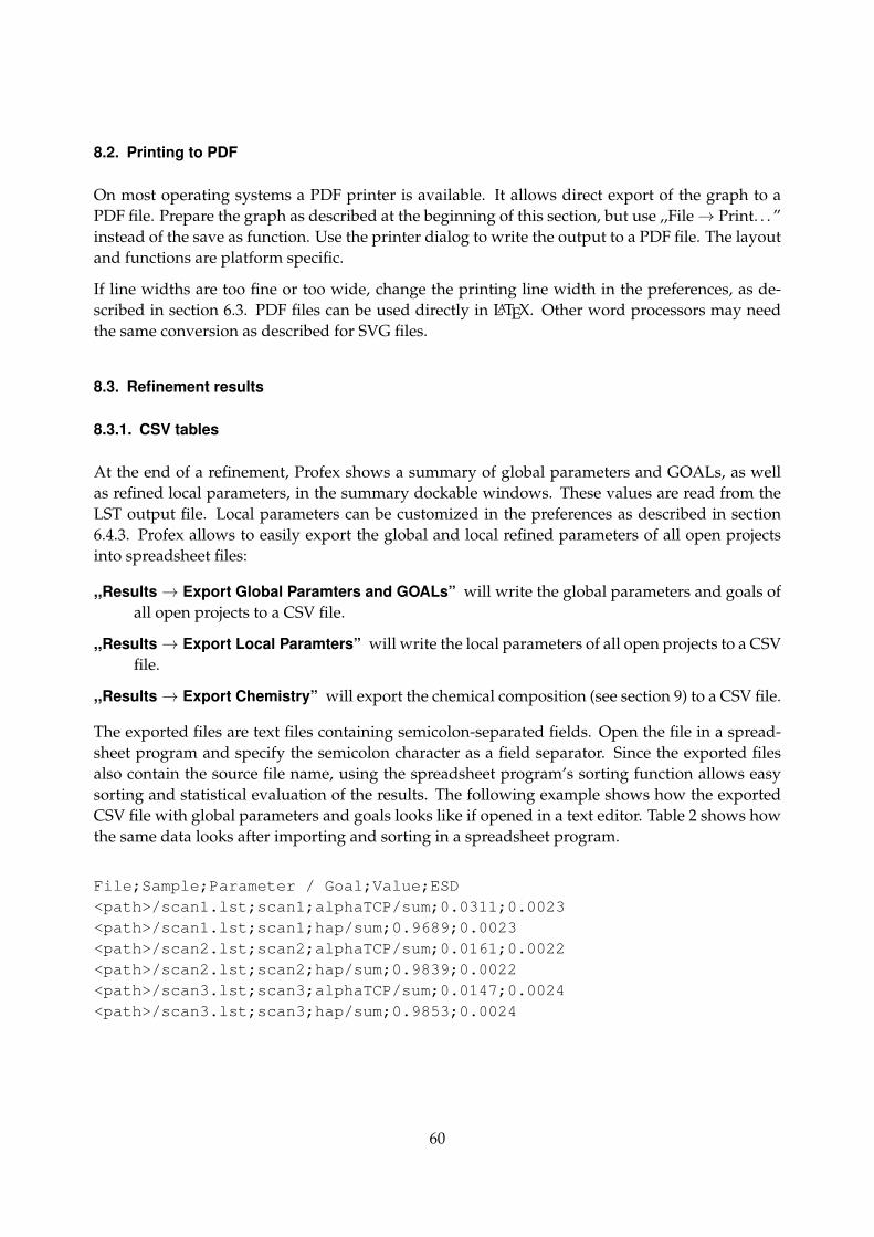
8.2. Printing to PDF

On most operating systems a PDF printer is available. It allows direct export of the graph to aPDF file. Prepare the graph as described at the beginning of this section, but use ,,File→ Print. . . ”instead of the save as function. Use the printer dialog to write the output to a PDF file. The layoutand functions are platform specific.

If line widths are too fine or too wide, change the printing line width in the preferences, as de-scribed in section 6.3. PDF files can be used directly in LATEX. Other word processors may needthe same conversion as described for SVG files.

8.3. Refinement results

8.3.1. CSV tables

At the end of a refinement, Profex shows a summary of global parameters and GOALs, as wellas refined local parameters, in the summary dockable windows. These values are read from theLST output file. Local parameters can be customized in the preferences as described in section6.4.3. Profex allows to easily export the global and local refined parameters of all open projectsinto spreadsheet files:

,,Results→ Export Global Paramters and GOALs” will write the global parameters and goals ofall open projects to a CSV file.

,,Results→ Export Local Paramters” will write the local parameters of all open projects to a CSVfile.

,,Results→ Export Chemistry” will export the chemical composition (see section 9) to a CSV file.

The exported files are text files containing semicolon-separated fields. Open the file in a spread-sheet program and specify the semicolon character as a field separator. Since the exported filesalso contain the source file name, using the spreadsheet program’s sorting function allows easysorting and statistical evaluation of the results. The following example shows how the exportedCSV file with global parameters and goals looks like if opened in a text editor. Table 2 shows howthe same data looks after importing and sorting in a spreadsheet program.

File;Sample;Parameter / Goal;Value;ESD<path>/scan1.lst;scan1;alphaTCP/sum;0.0311;0.0023<path>/scan1.lst;scan1;hap/sum;0.9689;0.0023<path>/scan2.lst;scan2;alphaTCP/sum;0.0161;0.0022<path>/scan2.lst;scan2;hap/sum;0.9839;0.0022<path>/scan3.lst;scan3;alphaTCP/sum;0.0147;0.0024<path>/scan3.lst;scan3;hap/sum;0.9853;0.0024

60

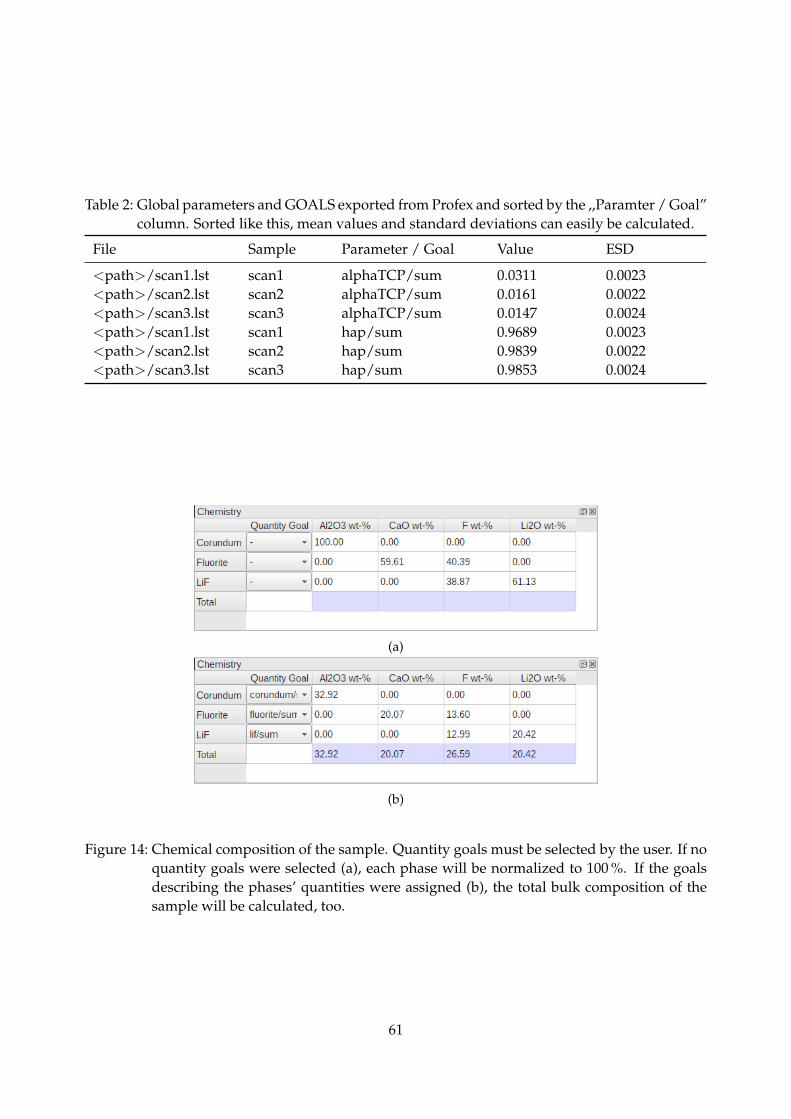
Table 2: Global parameters and GOALS exported from Profex and sorted by the ,,Paramter / Goal”column. Sorted like this, mean values and standard deviations can easily be calculated.

File Sample Parameter / Goal Value ESD

<path>/scan1.lst scan1 alphaTCP/sum 0.0311 0.0023<path>/scan2.lst scan2 alphaTCP/sum 0.0161 0.0022<path>/scan3.lst scan3 alphaTCP/sum 0.0147 0.0024<path>/scan1.lst scan1 hap/sum 0.9689 0.0023<path>/scan2.lst scan2 hap/sum 0.9839 0.0022<path>/scan3.lst scan3 hap/sum 0.9853 0.0024

(a)

(b)

Figure 14: Chemical composition of the sample. Quantity goals must be selected by the user. If noquantity goals were selected (a), each phase will be normalized to 100 %. If the goalsdescribing the phases’ quantities were assigned (b), the total bulk composition of thesample will be calculated, too.

61

9. Chemical composition

After the refinement, Profex will calculate the bulk chemical composition of the sample from thestructural information and refined site occupancies reported in the list file (*.lst). The elemen-tal composition, expressed in wt-% of the oxide, is shown in the ,,Chemistry” dockable widget(Fig. 14). In a first step, Profex will calculate the chemical composition of each phase, and nor-malize it to 100 % (Fig. 14a). In order to calculate the bulk composition of the entire sample, Profexneeds to know the relative quantity of each phase, which is normally calculated as a global goal.Profex will attempt to identify the correct ,,Quantity Goal” by comparing global goal names withthe phase name. If a goal name of format phase name/some string is found, with phase namematching the phases PHASE variable (case insensitive), the goal will be automatically selected.Else no ,,Quantity Goal” will be selected and the user will have to select it manually.

As an example, the following ,,Quantity Goal” will be recognized and assigned automatically,because the phase name and goal name match (matching is case insensitive):

STR file: PHASE=CorundumGOAL:corundum=GEWICHT

SAV file: GOAL[1]=corundum/sum

But the following ,,Quantity Goal” will not be recognized automatically, because the phase nameand goal name do not match. The user will have to select it manually:

STR file: PHASE=CorundumGOAL:Al2O3=GEWICHT

SAV file: GOAL[1]=Al2O3/sum

Once a valid ,,Quantity Goal” has been selected for a phase, the element composition will benormalized to the phase’s quantity. The total chemical composition will be calculated only whenall phases were assigned a valid ,,Quantity Goal” (Fig. 14b).

The oxides and their molecular weights used to calculate the composition can be accessed andcustomized in the preferences by calling ,,Edit → Preferences. . .→ Chemistry” (Fig. 15a). Ele-ments without molecular weight value, or with a value of 0.0, will be ignored for the calculation.It is recommended to leave the molecular weight of oxygen (element No. 8) empty or at 0.0 toavoid listing oxygen as a separate element in the chemistry output table. See section 6.7 for moreinformation on customizing the oxide parameters.

Select ,,Project→ Export Chemistry. . . ” to export the data to a csv file.

Clicking with the right mouse button on the table allows to copy the table to the clipboard. Thecontent can be pasted to a spread sheet program. The semicolon character ,,;” is used as fieldseparator. The entire table will be copied, cell selections will be ignored.

62

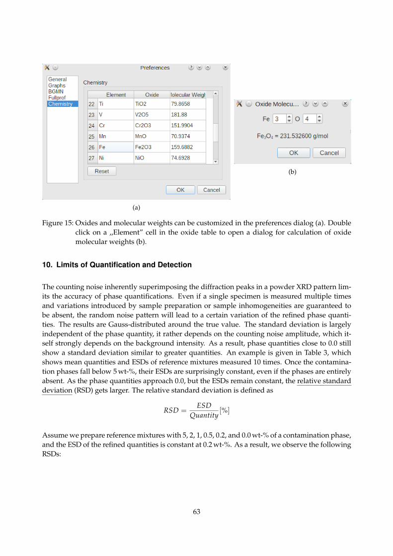
(a)

(b)

Figure 15: Oxides and molecular weights can be customized in the preferences dialog (a). Doubleclick on a ,,Element” cell in the oxide table to open a dialog for calculation of oxidemolecular weights (b).

10. Limits of Quantification and Detection

The counting noise inherently superimposing the diffraction peaks in a powder XRD pattern lim-its the accuracy of phase quantifications. Even if a single specimen is measured multiple timesand variations introduced by sample preparation or sample inhomogeneities are guaranteed tobe absent, the random noise pattern will lead to a certain variation of the refined phase quanti-ties. The results are Gauss-distributed around the true value. The standard deviation is largelyindependent of the phase quantity, it rather depends on the counting noise amplitude, which it-self strongly depends on the background intensity. As a result, phase quantities close to 0.0 stillshow a standard deviation similar to greater quantities. An example is given in Table 3, whichshows mean quantities and ESDs of reference mixtures measured 10 times. Once the contamina-tion phases fall below 5 wt-%, their ESDs are surprisingly constant, even if the phases are entirelyabsent. As the phase quantities approach 0.0, but the ESDs remain constant, the relative standarddeviation (RSD) gets larger. The relative standard deviation is defined as

RSD =ESD

Quantity[%]

Assume we prepare reference mixtures with 5, 2, 1, 0.5, 0.2, and 0.0 wt-% of a contamination phase,and the ESD of the refined quantities is constant at 0.2 wt-%. As a result, we observe the followingRSDs:

63

Quantity [wt-%] ESD [wt-%] RSD [%]

5.0 0.2 4.02.0 0.2 10.01.0 0.2 20.00.5 0.2 40.00.2 0.2 100.00.0 0.2 ∞

For small quantities the scattering of the values becomes excessively large compared to the meanvalue, which is expressed by huge RSDs. In other words, the refined quantity becomes unreliable.Many textbooks, guidelines and standards define the limits of quantification and detection (LOQand LOD) as a relative standard deviation. For example, they specify that for quantification themean value must be at least 4 times greater than its standard deviation, or the standard deviationmust be less than one quarter of the value (RSD ≤ 25%). And for detection, the mean value mustbe at least 2 times greater than its standard deviation, or the standard deviation must be less thanhalf the value (RSD ≤ 50%). The actual limits might depend on the source of the information.

The example in Table 3 also shows that, with the exception of phase C, none of the contaminationphases reach 0.0 wt-% in the sample absolutely free of contaminations (bottom line). Once thepeak intensities drown in the counting noise, the refinement algorithm will be able to fit positiveintensities into the noise pattern. This has some undesired side effects: These residual intensities,even when reported as ,,not detected”, reduce the quantity of the main phase, as long as they aretaken into the normalization of phase quantities to 100 %. In Table 3 the quantity of phase A isreduced to 99.10 wt-% due to accumulated residual intensities, even though no contaminationswere present. In order to avoid this problem, which can become even more pronounced if morenon-existent phases are added to the refinement, it is recommended to remove phases below thedetection limit from the project and repeat the refinement. This process should be repeated untilnone of the refined phases is below the detection limit. Profex’ facilitates this strategy by high-lighting phases below the detection and quantification limits and by showing a warning in thesummary table. The feature has to be enabled in the preferences dialog (Edit→ Preferences. . .→BGMN → Summary Tables → ,,Show warnings for values below detection and quantificationlimit”). In the same dialog the relative standard deviations (RSD) used as limits of quantificationand detection can be defined. In the example shown in Figure 16 the limit of quantification isreached when the refined quantity falls below 8 times its ESD (RSD ≥ 12.5 %), and the limit ofdetection is reached when it falls below 4 times its ESD (RSD ≥ 25 %).

Some phases actually converge towards 0.0 wt-% despite a considerable noise pattern. In thatcase the ESD may reach 0.0 wt-%, too. However, this is an artifact of the refinement algorithmand its error propagation, as there cannot be an absolute certainty of absence of a particular phaseas long as there is noise superimposing the diffraction signal. After all, there always might be asignal hidden in the noise. If the ESD reaches 0.0, the refined quantity might never fall below thequantification and detection limit, as the ESD shrinks along with the value rather than remainingconstant, and the RSD may or may not exceed the LOQ or LOD at a certain point. In order to avoidthis undesired result, Profex allows to define a minimum ESD. Any refined ESD below this value

64

will be considered to be an artifact, i. e. an unrealistically low ESD, and instead the minimum ESDspecified in the preferences dialog will be used. That way, a hard-coded minimum LOQ and LODis introduced. For example, the limit of detection in Figure 16 is defined as

LOD =ESDvalue

= 0.250

If we refine a phase quantity to 0.06 wt-% with an ESD of 0.01, its RSD is:

RSD =0.010.06

= 0.167

The RSD does not exceed the LOD, therefore the phase quantity of 0.06 wt-% should be considereddetectable, Profex will not show the warning ,,< LOD”. However, it is quite obvious that a quan-tity of 0.06 wt-% cannot be detected in most real datasets collected on conventional instrumentswith standard settings. Also an ESD of 0.01 wt-% is impossible to achieve if there is countingnoise in the pattern. The low ESD must therefore be an artifact. Applying Profex’ minimum ESDat 0.05 wt-% (which is a realistic choice), the equation changes as follows

RSD =minESD

0.06=

0.050.06

= 0.833

The RSD exceeds the LOD of 0.250 by far, and the quantity of 0.06 wt-% is flagged as ,,< LOD”. Infact, any quantity below

minESDLOD

=0.050.250

= 0.20

will be flagged as ,,< LOD”, regardless of its refined ESD.

If the minimum ESD is set to 0.0, the feature is deactivated and all refined ESDs will be used asread from the results file. This is not recommended. The minimum ESD should be set to a positivevalue. The non-existent phases B and D in Table 3 that converged to a positive residual intensity(bottom line) had residual ESDs of 0.06 and 0.14 wt-%. It is a reasonable guess to use a value justbelow the residual ESDs of non-existent phases as a minimum ESD. In this example, 0.05 wt-%seems to be a good choice.

65

Figure 16: Warnings for quantities below LOQ and LOD can be activated in the preferences dialog.Relative standard deviations (ESD/value) used as LOQ and LOD are also specified onthe same page.

66

Figu

re17

:Pro

fex

show

ing

war

ning

sfo

rph

ases

belo

wth

ede

tect

ion

limit

(<LO

D).

67

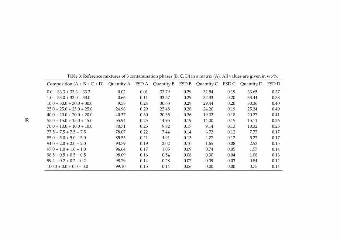
Table 3: Reference mixtures of 3 contamination phases (B, C, D) in a matrix (A). All values are given in wt-%.

Composition (A + B + C + D) Quantity A ESD A Quantity B ESD B Quantity C ESD C Quantity D ESD D

0.0 + 33.3 + 33.3 + 33.3 0.02 0.01 33.79 0.29 32.54 0.19 33.65 0.371.0 + 33.0 + 33.0 + 33.0 0.66 0.11 33.57 0.29 32.33 0.20 33.44 0.3810.0 + 30.0 + 30.0 + 30.0 9.58 0.24 30.63 0.29 29.44 0.20 30.36 0.4025.0 + 25.0 + 25.0 + 25.0 24.98 0.29 25.48 0.28 24.20 0.19 25.34 0.4040.0 + 20.0 + 20.0 + 20.0 40.37 0.30 20.35 0.26 19.02 0.18 20.27 0.4155.0 + 15.0 + 15.0 + 15.0 55.94 0.25 14.95 0.19 14.00 0.15 15.11 0.2670.0 + 10.0 + 10.0 + 10.0 70.71 0.25 9.82 0.17 9.14 0.13 10.32 0.2577.5 + 7.5 + 7.5 + 7.5 78.07 0.22 7.44 0.14 6.72 0.12 7.77 0.1785.0 + 5.0 + 5.0 + 5.0 85.55 0.21 4.91 0.13 4.27 0.12 5.27 0.1794.0 + 2.0 + 2.0 + 2.0 93.79 0.19 2.02 0.10 1.65 0.08 2.53 0.1597.0 + 1.0 + 1.0 + 1.0 96.64 0.17 1.05 0.09 0.74 0.05 1.57 0.1498.5 + 0.5 + 0.5 + 0.5 98.09 0.16 0.54 0.08 0.30 0.04 1.08 0.1399.4 + 0.2 + 0.2 + 0.2 98.79 0.14 0.28 0.07 0.09 0.03 0.84 0.12100.0 + 0.0 + 0.0 + 0.0 99.10 0.15 0.14 0.06 0.00 0.00 0.75 0.14

68

11. Profex-specific Control File Variables

Profex reads some additional variables from BGMN control files (*.sav) that are not mandatory forthe BGMN refinement backend. Some of them are only parsed by Profex and ignored by BGMN,and some of them are used for specific calculations of GOALs.

sum This variable is used to compute relative phase quantities normalized to 100 %. Normallyit holds the sum of the GEWICHT variables of all phases. If one phase is set as an internalstandard, the sum variable is used for the normalization to the internal standard quantity.sum is automatically managed by Profex if phases are added, removed, or set and unset asinternal standard.

ISTD Holds the phase name of the internal standard phase. It is only present if an internal stan-dard has been defined. It is added and removed by Profex if an internal standard is set orunset.

ISTDQ Holds the phase quantity of the internal standard phase normalized to 1.0 (not to 100 %).It is only present if an internal standard has been defined. It is added and removed by Profexif an internal standard is set or unset.

LOQ Relative standard deviation (ESD / value) considered as the limit of quantification (LOQ).This value will override the value set in the preferences dialog. It will only be parsed if theoption ,,Show warnings for values below detection and quantification limit” is set active inthe preferences dialog. If the ratio ESD / value of a refined phase quantity exceeds LOQ,it will be highlighted in the summary table and a warning ,,< LOQ” will be shown. Seesection 10 for more information.

LOD Relative standard deviation (ESD / value) considered as the limit of detection (LOD). Thisvalue will override the value set in the preferences dialog. It will only be parsed if theoption ,,Show warnings for values below detection and quantification limit” is set active inthe preferences dialog. If the ratio ESD / value of a refined phase quantity exceeds LOD,it will be highlighted in the summary table and a warning ,,< LOD” will be shown. Seesection 10 for more information.

MINESD Sets the minimum ESD that is considered realistic for refined phase quantities. This vari-able overrides the value set in the preferences dialog ,,Minimum ESD (ignore ESDs below)=”. See section 10 for more information.

69

12. Scan batch conversion

Several scan files can be converted to other data formats at a time using the ,,File → Scan batchconversion. . . ” feature. However, due to limitations given by the formats, SVG and pixel images(PNG) are not available for batch conversion.

When opening the batch conversion dialog by clicking ,,File→ Scan batch conversion. . . ”, the filequeue will contain all currently opened scan files by default. More files can be added by clickingthe ,,Add File” button and selecting one or more files, and selected files can be removed from thequeue by clicking the ,,Remove File” button.

Some output format support multiple scans stored in a single file. The option ,,Write scans to onefile” will instruct Profex to store all scans found in a source file into one single file. In that case, allscans Iobs, Icalc, Idi f f , Ibackground, and all sub phase patterns found in a DIA file will be stored in asingle output file. Use ,,Write scans to individual files” to write these patterns into single outputfiles instead. Note that storing multiple scans in one file must be supported by the output formatas well as by Profex’ output filter, which is currently only the case for ASCII and Gnuplot files.

Click ,,Convert” to start the conversion process, or ,,Close” to close the dialog without conver-sion. Output files will be stored at the location of their source files using the same base file name.Existing output files will be overwritten without warning.

70

13. CIF and ICDD XML import

Crystal structure files retrieved from online or commercial databases are usually supplied in theCIF format [10] or in an XML file format if exported from the ICDD PDF-4+ database. Beforethey can be used with BGMN, the structure information needs to be converted the the BGMN STRfile format. Profex provides support to facilitate the conversion process for both CIF and XMLformats. PDF-4+ XML files are usually complete and require very little user input. CIF files, onthe other hand, often lack important information and require manual revision. The import andconversion process in Profex is identical to both CIF and XML formats. The following instructionsshow how to convert a CIF file to a BGMN STR file using Profex’ CIF import feature.

1. Retrieve a CIF file from an external resource (online or local database).

2. Start Profex and choose ,,File→ Import CIF. . . ” to open the CIF file.

3. If no space group number was found in the CIF file, Profex will display a dialog to selectthe number (Fig. 18a). Select the space group number of your structure. It has to be knownor determined from an external source. The field ,,Supported Settings” shows all HermannMauguin symbols of the selected space group number. The correct number must contain asymbol remotely similar to the symbol read from the CIF file. Due to the lack of standard-ization, CIF and BGMN Hermann Mauguin symbols often look similar, but not identical.

4. If more than one space group setting is available, select the correct one from the dialogshown in Fig. 18b. Again, the available Hermann Mauguin symbol often looks similar butnot identical to the one read from the CIF file.

5. The STR file will be created and shown in an editor (Fig. 19). Most likely the STR file is in-complete due to information missing in the CIF file. Some warnings are issued in the dialog.Check manually for complete information. Typically Wyckoff sequences and element typesare often missing.

The dialog also shows the original CIF file on a second tab. It may be useful to verify the STRfile or to retrieve more information if it was not extracted automatically. The XML file shownon the third tab is the intermediate format used by Profex. It is only shown for debuggingpurposes.

6. Once the STR file is complete, choose ,,Save STR” to save the file in the structure file databasedirectory.

Sometimes it is helpful to browse the space group numbers and symbols in the form supported byBGMN. Open ,,Help→ BGMN SPACEGRP.DAT” to open a dialog which shows all space groupnumbers, settings, and Wyckoff sequences in the nomenclature used by BGMN (Fig. 20).

The assignment CIF file tags to STR parameters is described in Table 4.

71

(a) Space group number (b) Space group setting

Figure 18: Importing a CIF file: If no space group number is found in the CIF file, it has to beentered manually in dialog (a). If more than one setting for the space group is available,it has to be choosen manually from dialog (b).

13.1. Automatic conversion of thermal displacement parameters

During the conversion from CIF to STR format Profex automatically transforms the thermal dis-placement parameters to the format supported by BGMN. Depending on the source format, thefollowing conversions are calculated (anisotropic βij values are not supported by the CIF for-mat.):

Isotropic B: Isotropic B is the format supported by BGMN. However, BGMN uses a differentunit than normally provided in the CIF file. Automatic conversion therefore performs thefollowing conversion:

Biso[nm2] = 0.01 · Biso[A2]

Anisotropic Bij: Anisotropic Bij are converted to isotropic B values in the expected unit [15]:

Biso[nm2] = 0.01 · 13 ∑

i∑

jBija∗i a∗j Ai Aj

with reciprocal lattice parameters a∗[A−1] and real lattice parameters A[A].

Anisotropic Uij: Anisotropic Uij are converted to Uequiv using the expression [15]:

Uequiv =13 ∑

i∑

jUija∗i a∗j Ai Aj

with reciprocal lattice parameters a∗[A−1] and real lattice parameters A[A]. Uequiv is con-verted to Biso by the following equation.

Isotropic Uequiv: Isotropic Uequiv values are converted to isotropic B:

Biso[nm2] = 0.01 · 8.0 · π2 ·Uequiv

72

Figure 19: After importing a CIF file and adding all space group information, the STR file is dis-played. It may still be incomplete. Check the warnings at the bottom of the dialog andfix the STR file text manually. The CIF file is also shown in the second tab for compar-isong. The XML file in the third tab is only used internally by Profex.

Figure 20: ,,Help→ BGMN SPACEGRP.DAT” opens a dialog to browse all space group numbers,settings, and atomic positions.

73

CIF File STR File

chemical name mineral PHASE=namechemical name common PHASE=namechemical name systematic PHASE=namedatabase code [a-z] Reference=namechemical formula [a-z] Formula=namesymmetry Int Tables number SpacegroupNo=numberspace group IT number SpacegroupNo=numbersymmetry space group name H-M HermannMauguin=symbolspace group name H-M alt HermannMauguin=symbolcell length a / b / c A= / B= / C=valuecell angle alpha / beta / gamma ALPHA= / BETA= / GAMMA=valueatom site label E=M±n(value)atom site type symbol E=M±n(value)atom site Wyckoff symbol Wyckoff=symbolatom site occupancy E=M±n(value)atom site fract x / y / z x= / y= / z=valueatom site B iso or equiv TDS=valueatom site U iso or equiv TDS=valueatom site aniso U [1-3] TDS=valueatom site aniso B [1-3] TDS=value

Table 4: Assignment of CIF parameter tags to BGMN STR variables.

74

14. Instrument configurations

Raytraced geometric peak profiles must be calculated by BGMN prior to refinement. The instru-ment configuration is described in a control file, and the two programs GEOMET and MAKEGEQ,which are part of the BGMN software distribution, are used to calculate and interpolate the peakprofile in a specific 2θ range. For more information please refer to the BGMN documentation [1].

Profex allows editing instrument control files in a simple text editor, and runs GEOMET andMAKEGEQ to generate the output files. A common workflow to modify an existing device con-figuration is shown below.

1. Run Profex and click ,,Instrument→ Edit Configuration. . . ”. Profex will open a file dialog inthe Device database directory. Select the instrument control file (*.sav) you intend to modify.

2. The instrument dialog shown in Fig. 21 will be shown. Edit the file as intended.

3. Save the file under a new name using the dialog’s ,,Save As” button. Be sure to save it in adirectory with write access.

4. Check the options ,,Raytrace (GEOMET)” and ,,Interpolate (MakeGEQ)”. The option ,,Cal-culate Profile (GERTEST)” is optional.

5. Check the option ,,Create Template for Refinement Control File” and select your tube’s targetmaterial and the type of monochromator you use.

6. Click the ,,Run” button and wait until the progress dialog has completed. Depending onhardware, simulated angular range, and device configuration, this process may take severalminutes to complete.

Once the process has completed, BGMN has created two new files (*.ger and *.geq), which are re-quired for refinements. If they were created outside of the Device database directory, they shouldbe moved there in order to appear in the ,,Add Phase” dialog. It is also recommended to manuallycreate a template file for the new configuration, as described in section 3.4.3.

Using ,,Instrument→New Configuration. . . ” will allow to read some hardware information fromBruker RAW V4, Bruker BRML V5, and PANalytical XRDML files to create a BGMN instrumentconfiguration file from scratch. Other raw data formats are not supported. Usually several vari-able required by BGMN will still not be available from the raw data files and will thus have to beentered manually.

The resulting theoretical peak shape computed by GERTEST and MakeGEQ can be displayed byclicking ,,Instrument → Show Peak Shape. . . ”. In the dialog click the button ,,Load InstrumentControl File” at the bottom left and load your instrument *.sav file. After computing the peakshape, the horizontal slider can be used to skip through the 2θ range and show the peak shape(Fig. 22). Displayed peaks can be exported to various formats using the export buttons at thebottom left.

75

Figure 21: ,,Instrument → Edit Configuration. . . ” opens a dialog to edit an existing instrumentconfiguration.

76

Figure 22: ,,Instrument→ Show Peak Shape. . . ” opens a dialog display the theoretical peak shapecomputed for a specific instrument configuration.

15. Scan File Handling

In contrast to the BGMN Rietveld backend, which only supports a limited number of scan file for-mats natively, Profex reads a wide and growing range of file formats. When running a refinementon a scan file format not supported by BGMN, Profex will by default automatically convert the filein the background and modify the control file accordingly. This section describes the conversionprocess and the settings allowing the user to control the conversion.

Automatic scan file conversion can be switched on and off in the preferences dialog by checkingor unchecking the option ,,Edit→ Preferences. . .→ BGMN→ Convert raw scans to XY format”.Scan file handling by Profex will be different depending on this setting. Unless conversion is notdesired for specific reasons, users are strongly advised to activate this option.

It is a surprisingly complex task to determine the correct file name of a project’s raw scan (VAL[n]keyword in the control file). The possible scenarios to be considered are manifold. Profex hassophisticated routines to determine the best guess for a VAL file name under all circumstances.These routines are illustrated in Figures 24–27.

In principle, when creating a new project, a raw scan file as obtained from the instrument is openedand a new control file is created either by using the ,,Add a new phase” dialog or the ,,Copy con-trol file” function (see section 4). Either way the loaded raw scan file determines the location andthe base name of the project, and all input and output file names in the control file will automat-ically be set to this scan’s file base name. More information on file name handling is given insection 3.4.3. The scan file name to be read by the BGMN Rietveld backend is specified with theVAL[n]=ScanFile.xxx line in the control file. The scan file name is given by the project name,

77

as described above, but the file format and extension is determined by Profex automatically, de-pending on the raw scan format and the setting of ,,Edit → Preferences. . .→ BGMN → Convertraw scans to XY format”. If a format natively supported by BGMN is detected, the file will be usedwithout conversion. If the format is not supported, the behavior will depend on the setting ,,Con-vert raw scans to XY format”: If active, the file will be converted to *.xy format and the VAL[n] fileentry will be adapted accordingly. If inactive, no conversion will be done and it is in the user’sresponsibility to guarantee correct file names and formats. See Fig. 23 for more explanations.

However, the processes described above represent relatively simple scenarios, when the raw scanfile is opened and the format and file name are known. In many situations it gets a lot trickierto determine the correct file name. The following situation represents a worst case: A DIA file isopened, conversion to *.xy is inactive, and the control file is created from another project using the,,Copy control file” feature. Normally, when a DIA file exists, a control file should also exist witha valid VAL[n] entry. However, when sharing or moving DIA files, or when the base name of theDIA and control file do not match, it may still occur that a DIA file is present but the correspondingcontrol file cannot be located. Trying to find the correct raw scan file used to create die DIA file isdifficult in such a situation:

1. The control file copied over from another project contains input and output file names (VAL,DIAGRAMM, OUTPUT, etc.) of the source project. All file names must be changed to thedestination project. The VAL file name found in this control file must not be used.

2. The displayed scan is a DIA file, which cannot be used as input file.

3. Converting the DIA file to *.xy is not allowed.

4. There is no reference to the raw scan in any of the available files.

5. In that case, Profex will scan the directory of the DIA file for a raw scan file in a formatnatively supported by BGMN. But there is no guarantee that such a file is found.

This is one of many scenarios when finding the correct VAL file name is not trivial. However,the complex processes illustrated in Figures 24–27 cover most situations, and if no solution can befound, a warning will be issued.

78

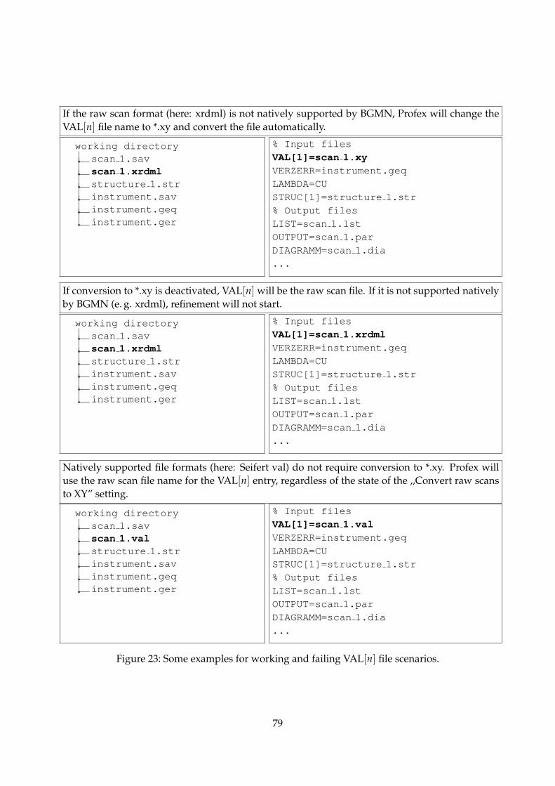
If the raw scan format (here: xrdml) is not natively supported by BGMN, Profex will change theVAL[n] file name to *.xy and convert the file automatically.

working directoryscan 1.savscan 1.xrdmlstructure 1.strinstrument.savinstrument.geqinstrument.ger

% Input filesVAL[1]=scan 1.xyVERZERR=instrument.geqLAMBDA=CUSTRUC[1]=structure 1.str% Output filesLIST=scan 1.lstOUTPUT=scan 1.parDIAGRAMM=scan 1.dia...

If conversion to *.xy is deactivated, VAL[n] will be the raw scan file. If it is not supported nativelyby BGMN (e. g. xrdml), refinement will not start.

working directoryscan 1.savscan 1.xrdmlstructure 1.strinstrument.savinstrument.geqinstrument.ger

% Input filesVAL[1]=scan 1.xrdmlVERZERR=instrument.geqLAMBDA=CUSTRUC[1]=structure 1.str% Output filesLIST=scan 1.lstOUTPUT=scan 1.parDIAGRAMM=scan 1.dia...

Natively supported file formats (here: Seifert val) do not require conversion to *.xy. Profex willuse the raw scan file name for the VAL[n] entry, regardless of the state of the ,,Convert raw scansto XY” setting.

working directoryscan 1.savscan 1.valstructure 1.strinstrument.savinstrument.geqinstrument.ger

% Input filesVAL[1]=scan 1.valVERZERR=instrument.geqLAMBDA=CUSTRUC[1]=structure 1.str% Output filesLIST=scan 1.lstOUTPUT=scan 1.parDIAGRAMM=scan 1.dia...

Figure 23: Some examples for working and failing VAL[n] file scenarios.

79

Start ,,Generate de-fault control file” in,,Add Phase” dialog

Temporarily store pre-vious VAL[n] = file

name if available

Apply control file con-tent from template

Previous VAL filename available?

VAL[n] = previous VAL file

VAL[n] = remains empty

Proceed to ,,Verify VAL file”

yes

no

Figure 24: VAL file handling when calling the ,,Add Phase” dialog and activating the option ,,Gen-erate default control file” to create a control file from a template file.

80

Start ,,Copy control file”Temporarily store

file name of previousVAL[n] = entry if available

Apply new con-trol file content

Previous VAL[n] =empty?

VAL[n] = previous VAL file

Convert to *.xy?VAL[n] = dis-played scan file

Disp. scan file =native BGMN

format?

VAL[n] = dis-played scan file

Search natively supportedfile with the same base

name at the same locationas the displayed scan file

Alternative scan filefound?

VAL[n] = alter-native scan file

Leave VAL[n] =

empty, display warningProceed to ,,VALfile verification”

no

yes

yes

no

yes

no

yes

no

Figure 25: VAL file name handling when using the ,,Copy control file” function.

81

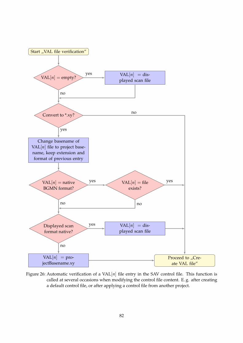
Start ,,VAL file verification”

VAL[n] = empty?VAL[n] = dis-played scan file

Convert to *.xy?

Change basename ofVAL[n] file to project base-name, keep extension andformat of previous entry

VAL[n] = nativeBGMN format?

VAL[n] = fileexists?

Displayed scanformat native?

VAL[n] = dis-played scan file

VAL[n] = pro-jectBasename.xy

Proceed to ,,Cre-ate VAL file”

yes

no

yes

no

yes

no

yes

no

yes

no

Figure 26: Automatic verification of a VAL[n] file entry in the SAV control file. This function iscalled at several occasions when modifying the control file content. E. g. after creatinga default control file, or after applying a control file from another project.

82

Start ,,Create VAL file”

VAL[n] = file existson hard disk?

Convert displayedscan file to *.xy

Launch BGMN re-finement process

yes

no

Figure 27: Immediately before running the refinement process, Profex checks whether the VALfile referenced in the control file exists on the hard disk. If not, a *.xy file will be createdfrom the currently displayed scan file.

83

A. Bundle File Structure

A.1. Windows

Profex-BGMN-Bundle-3.9.0.zipBGMNwin

BGMN.EXEMakeGEQ.EXE...

Profex-3.9.0Devices

Instrument 1.savInstrument 1.gerInstrument 1.geqInstrument 1.tplInstrument 2.sav...

StructuresStructure 1.strStructure 2.str...

PresetsPreset 1.pfpPreset 2.pfp...

profex.exe...

A.2. Mac OS X

Profex-BGMN-Bundle-3.9.0.dmgProfex-BGMN

profex.appBGMNwin

bgmnmakegeq...

BGMN-TemplatesDevices

Instrument 1.savInstrument 1.gerInstrument 1.geqInstrument 1.tplInstrument 2.sav...

StructuresStructure 1.str

84

Structure 2.str...

PresetsPreset 1.pfpPreset 2.pfp...

A.3. Linux

An RPM file for OpenSuse Leap 42.1 x86 64 is provided with the following file structure./

optProfex-BGMN

Profexprofexprofex.png

BGMNwinbgmnmakegeq...

BGMN-TemplatesDevices

Instrument 1.savInstrument 1.gerInstrument 1.geqInstrument 1.tplInstrument 2.sav...

StructuresStructure 1.strStructure 2.str...

PresetsPreset 1.pfpPreset 2.pfp...

usrshare

applicationsprofex.desktop

85

References

[1] http://www.bgmn.de/

[2] https://www.ill.eu/sites/fullprof/

[3] http://profex.doebelin.org/

[4] http://qt-project.org/

[5] http://www.zlib.net/

[6] http://quazip.sourceforge.net/

[7] http://support.apple.com/kb/ht3696/

[8] Andrew, V.J. ,,The Re1ative Intensities of the Lα1, β1, β2, and γ1, Lines in Tantalum, Tungsten,Iridium, and Platinum”. Phys. Rev. 42(5), 591 (1932).

[9] http://www.castep.org/

[10] http://www.iucr.org/resources/cif/spec/version1.1/cifsyntax/

[11] http://users.uoi.gr/nkourkou/powdll/

[12] http://www.gnuplot.info/

[13] http://plasma-gate.weizmann.ac.il/Grace/

[14] http://fityk.nieto.pl/

[15] Fischer, R.X., Tillmanns, E. The equivalent isotropic displacement factor. Acta Cryst. C44, 1988,775–776.

86

Index

Bij, 72Biso, 72Uequiv, 72Uij, 72

Abort, 35About Profex, 37Add Phase, 16, 34, 49Anisotropic, 30AntiAliasing, 39ASCII free format, 56ASCII HKL list, 57Atomic Scattering Factor, 37Axis

Font Labels, 40y-axis Scaling, 39

B1, 43Backend, 6, 21, 22Backup, 35Batch Conversion, 32, 70Batch Refinement, 35BGMN Variables, 37BGMN.EXE, 8, 11, 40BGMNwin, 8Brindley, 44

Chemical Composition, 19Chemical composition, 22Chemistry, 22, 62CIF File

Import, 32, 71Color, 21Context Help, 18, 22, 37Context menu, 28Control file, 28Convergence, 22, 37Coordinates, 26Copy Control File, 33Counting Noise, 25CPU Cores, 38Cross Hair, 25Cursor, 25Custom Profile Function, 43

Default Control File, 16, 49Default Project Type, 38Device Configuration, 13Device Database, 9, 11, 13, 41Displacement

Left, 34Reset, 34Right, 34Vertical, 34

Dockable Window, 18, 19, 23Closing, 19Detaching, 19Moving, 19Opening, 19Stacking, 19

Double Click, 26

EPS, 18Export, 36, 56

CELL, 36Chemistry, 36CIF, 36Global Parameters, 36Graphs, 56Local Parameters, 36Results, 16, 60

Find, 33First Steps, 16Fityk, 59Fix parameter, 30Font, 38

Axis Labels, 40hkl Indices, 40Legend, 40Title, 40

GEOMET.EXE, 11, 40, 75GERTEST.EXE, 11, 41GEWICHT, 43Gnuplot, 58GOAL, 18, 21, 22, 36, 37, 43Grace, 58Graph File

Open, 31

87

Remove, 32Save, 32Save As, 32

GraphFileOpen, 16

Grid lines, 39

hkl Indices, 21, 24, 34, 47Font, 40Range, 47

ICDDImport, 32

ImportCIF File, 71ICDD XML, 71

Insert Scans, 32Installation, 6

Bundle, 6Compiling, 7Linux, 6Mac OS X, 7Windows, 6

Instrument, 36Instrument Configuration, 16, 36, 49, 75Internal Standard, 35Isotropic, 30

k1, 43k2, 43

Legend, 24, 34Font, 40

Line Style, 21Line Width, 21

Display, 39Printing, 39

List Coordinates, 26

Main Window, 18, 20, 24MAKEGEQ.EXE, 11, 40, 75Margin Color, 33, 39, 40Menu, 31Menu Bar, 18Micro-Absorption, 44Multi-Scan Files, 39

Open file, 28

OUTPUT.EXE, 11, 40

ParametersChemistry, 36, 37Global, 18, 21, 36, 37Local, 18, 22, 36, 37

PDF, 60Phase

Add, 49Remove, 49

Phase Pattern, 21, 24, 33Pixel Image, 57, 70Plot, 33Plot Area, 18, 24Plot Options, 18, 21, 37PNG, 57, 70Preferences, 33, 38

BGMN, 40Chemical Composition, 47Fonts, 40Fullprof, 46General, 38Graph, 39Limits, 44Reference Structure, 47Scan Styles, 40Structure File Handling, 43Summary Table, 44Text Blocks, 48Text Editors, 38

Preset Database, 9, 11, 14, 51Presets, 14, 35, 51Presets Database, 41Print, 32, 60profex.exe, 8Project, 34

Close, 32Close All, 32Organization, 50

Projects, 18, 19, 37

Quit, 32

RecentGraph Files, 32Text Files, 32

Redo, 33Reference Structure, 26, 31, 47

88

Automatic Indexing, 47Clear Buffer, 47hkl Range, 47Index, 31Reset, 31

Refine parameter, 30Refinement, 35

Abort, 35Run, 16, 35Run Batch, 35

Refinement Protocol, 18, 21, 37Remove Phase, 16, 34, 49Remove Scan, 32Replace, 33Reset File, 33Restore open projects, 38Results, 36RP, 43Run, 35

Scalable vector graphics, 58, 70Scaling, 39Scan

Insert, 32Remove, 32

Scan Style, 40Color, 40Point Style, 40

Setup, 8Automatic, 8Linux, 8Mac OS X, 9Manual, 9Windows, 8

SPACEGRP.DAT, 37, 71Spectral line cursor, 25, 42Stacking, 28

Left, 34Reset, 34Right, 34Vertical, 34

Status Bar, 19STR File Handling, 12Structure, 49Structure Database, 9, 11, 41Structure File, 50

Close All, 35

Open All, 34Structure file, 30SVG, 58, 70Switch to

Control File, 33Graph, 33Output File, 33

Symbol Size, 39

TDS, 72Template, 13Template File, 11Text Blocks, 33Text Editor, 18Text File

Open, 31Save, 32Save As, 32

Thermal Displacement Parameters, 72Thumbnail, 39Title

Font, 40Tool Bar, 18, 31

Layout, 38Main Tool Bar, 18Project Tool Bar, 18Reference Structure, 31Reference Structure Tool Bar, 18Refinement Tool Bar, 18

Tungsten, 25

Un-Zoom, 25Undo, 33User Interface, 18

VERZERR.EXE, 41View, 33Visibility, 21

Wavelength, 38, 42Window, 37WINE, 11, 41

XMLImport, 32

XML FilImport, 71

Zoom, 25, 33

89

Zoom Range, 33

90