prof. haim wolfson structural bionformatics 2004

Structural Bionformatics 2004 Prof. Haim Wolfson


Flexible Docking - general methodology

Major approaches :

• Rigid subpart docking (place and join):– Split the flexible molecule into rigid subparts.– Dock independently each subpart.– Pair the top hypotheses for each subpart to detect

hinge consistency.Example : Des Jarlais, Sheridan, Dixon, Kuntz,

Venkatraghavan (1986).


• Incremental construction method :– Position a ‘preferred’ anchor fragment. – Rotate sequentially the flexible bonds to position the

other fragments.Example: Leach & Kuntz (1992); Lengauer et al. - FLEXX.

• Hinge scoring method:– Incorporate bond information already in the initial

filtering steps by accumulating information at the hinges. – No preference for specific parts. Reminds the place and

join method yet exploits the consistency of neighboring part placement in the initial stages.

Example : Sandak, Nussinov, Wolfson (1995).


Search in multi-dimensional degrees of freedom (torsion angle) space :

• Evolutionary/Genetic Algorithms : – Represent degrees of freedom as strings.– Create offsprings by (genetic) combination of parents.– Re-evaluate fitness of each string and prune “weak”

hypotheses.– Jones et al. J. Mol. Bio . Vol 245 (1995), pp. 43-

….• Simulated Annealing :

AutoDock – Goodsell et al. Proteins 1990.


GGH based flexible docking

Applies either to flexible ligands or to flexible receptors.


General Algorithm outline

Can be applied either to a dataset of ligands vs a receptor or a dataset of receptors vs. a ligand.

• Calculate the molecular surface of the receptor and the ligands and their interest points (+ normals).

• Match the interest points and recover candidate multi-transformations.

• Check for inter-molecule and intra-molecule penetrations and score the amount of contact.

• Rank by energies.


Point Matching algorithm- prepr.• For each database molecule :

– Define r.f.’s at every hinge.– For each minimal feature (e.g. triplet) compute an r.f.

and shape signature.– For each (triplet based) reference frame compute the

transformation btwn that frame and the hinge based frame and store (molec., part, r.f., transf.) in a hash (lookup) table at an entry addressed by the r.f. shape signature.


Point Matching algorithm-recognition

• For the target molecule :– For each minimal feature compute an r.f. and shape

signature.– Access the table by the shape signature, and for

each transformation appearing there :• transform the r.f. to ‘hypothesized’ hinge position;• advance the counter of that hinge location for the appropriate

molecule and part.

– Check highest scoring hinges .– Verify the resulting transformations .


Flexible DockingCalmodulin with M13 ligand


Flexible Docking HIV Protease Inhibitor


The FlexX Algorithm

• Rarey, …, Lengauer. J. Mol. Bio., vol. 261, (1996), pp. 470-

• An incremental construction algorithm


The general schema

Incremental construction

Scoring function

Receptor-ligand interactions

Ligand conformational flexibility

Modeling

Algorithm

Base selection

Base placement


The Ligand conformational flexibility

• Approximated by a discrete set of conformations.– rotatable single bond - modeled by a

discrete set of preferred torsion angles from the MIMUMBA DB.

– Ring system - A set of ring conformations is computed with the program CORINA.


The model of receptor-ligand interactions

• Modeled by a few special types of interactions

• hydrogen bonds• metal acceptors bonds• hydrophobic contacts


The model of protein-ligand interactions – Cont.

• To each interaction group, we assign:– Interaction types – Interaction geometry ( center + surface)


Two groups interact if :• The centers of the groups lie approximately on the

surface of the counter group.• The interaction types are compatible

• The intermolecular interactions can be classified by the strength of their geometric constrains


Scoring function• Estimates the free binding energy in the complex

• The function is additive in the ligand atoms.

match score

contact score


Overall docking algorithm

1. Ligand fragmentation2. Select & Place a set of base fragments3. Construct the ligand by linking the

remaining fragments.


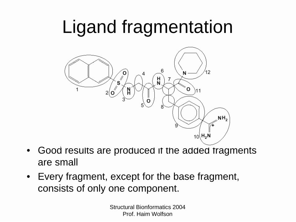
Ligand fragmentation

• The ligand is decomposed into components by cutting at each acyclic bond.

• Fragmentation is a partition of the components of the molecule, such that every part, called fragment, is connected in the component tree.


Ligand fragmentation

• Good results are produced if the added fragments are small

• Every fragment, except for the base fragment, consists of only one component.


Selecting a base fragment

• The problem: Find a fragment which leads to low energy docking solution.

• Good base fragment properties:– Placeability– Specificity


Selecting a base fragment –Cont.• We look for fragments maximizing the

function:


Rules for selecting a set of fragments

• No base fragment is fully contained in another base fragment

• Each component occurs in at most two base fragments

• Each component in a base fragment must be either necessary for the connectivity of the fragment or it must have interaction centers.


The base placement algorithm

• Goal: find positions of the base fragment in the active site such that sufficient number of favorable interactions between the fragment and the protein can occur simultaneously.

• Solution: pose clustering.


The base placement algorithm –Cont.

• Preparation: Store all triangles of interaction points (IP) of the protein in a hash table.

• Find all the compatible fragment IP’s triangles.

• Clustering of the legal transformations


The incremental construction algorithm

• Input: solution set - set of partial placements with the ligands constructed up to and including fragment i-1

• Output: set of partial placements with the ligands constructed up to and including fragment i


The complex construction algorithm – cont.

• Adding the next fragment in all the possible conformations

• Reject extended placements that have strong overlap with the receptor or internal overlap with the ligand.

• Searching for new interactions• Optimizing the positions of the partial ligand• Selecting a new solution set• Clustering the solution set


Optimizing the positions of the partial ligand

• The placement is optimized when:– New interactions are found.– The placement contains slightly overlapping

atoms between the receptor and the ligand.

( )2

rlw iii −∑


Selecting a new solution set

• Select k best-scoring solutions• Problem: the scoring values cannot be

compared directly when different fragments are involved.

• Solution: estimate the score of the whole ligand, given a partial placement.


Clustering partial solutions

• If no placement contains the other, the distance is infinity

• Otherwise, the distance is defined to be the RMSD of the intersecting atoms.

• A cluster is reduced to a single placement.


Exploring receptor Flexibility


Protein flexibility - motivation• Induced fit – side chain or even backbone

adjustments upon docking of different ligands to the same protein.

• Even small conformational changes are critical for docking applications e.g. if a rotatable bond prevents a ligand from binding in the correct position.


Protein flexibelity• Main idea: describe the protein structure

variations with a set of protein structures representing the flexibility, mutation or alternative models of a protein.

• The variability considered by FlexE is defined by the differences within the given input structures.


United protein description

• Data structure that handles the protein structures variations.

• Contains an ensemble of up to 30 possible conformation of the protein.

• Most of them are low energy conformations of the same protein.


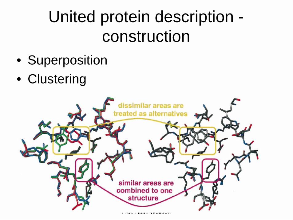
United protein description -construction

• Superposition• Clustering

Add picture - 8


Notation

• Component : all the atoms which belong to the same amino acid or mutation of the amino acid. Contains a backbone part and a side chain part

• Part : set of instances• Instance : one of the

alternative conformations.


United protein description -clustering

• The superimposed structures are combined by clustering each part separately

• Complete linkage hierarchical cluster• The clustered instances can be

recombined to form new valid protein structures.


Incompatibility

• Two instances of the united protein description are incompatible if they cannot be realized simultaneously. – Logical: two instances are

alternative to each other– Geometric: two logically

compatible instances overlap– Structural: two instances of

the same chain are unconnected


Incompatibility graph

{ }}bleincompatiaandE

cesinsV

vve jiij=

= tan


Incompatibility graph• The incompatibility is

internally represented as a graph by using the instances as nodes and the connecting pairs of incompatible nodes by an edge.

• Valid protein structures correspond to independent sets in the graph.


Selection of instances

• The ligand is placed fragment by fragment into the active site by the incremental construction algorithm.

• After each construction step, all possible interactions are determined.

• Apply the scoring function for each instance.

• We chose the IS with the highest score.


• The IS can be assembled from IS of the connected components.

• Apply a modified version of the Bron-Kerbosch algorithm.

Select the optimal IS


Evaluation

• FlexE was evaluated with ten protein structures ensembles containing 105 crystal structure from the PDB.

• The structures within the ensemble – highly similar backbone trace– Different conformations for several side

chains.


Evaluation – Cont.

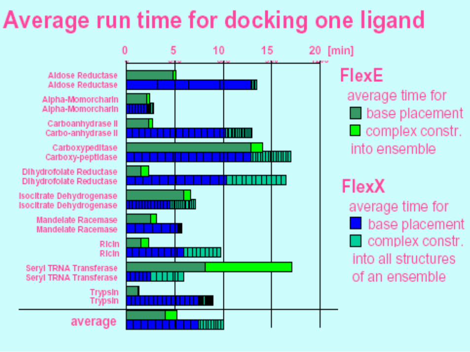
• FlexE finds a ligand position with RMSD below 2 A in 67% of the cases.

• Average CPU time for the incremental construction algorithm is 5.5 minutes.


Discussion

• The ensemble approach is able to cope with several side-chains conformations and even movements of loops.

• Motions of larger backbone segments or even domains movements are not covered by this approach.


FlexDockFlexDock: Algorithm Stages: Algorithm Stages

Rigid Parts Docking via Geometric Hashing

BB

Assembly of partial dockings into a flexible result

AA

AA

AAAA

BBAA

AA


Flexible Assembly StageFlexible Assembly Stage

NODE: NODE: transformation, scoretransformation, score

Part 1 resultsPart 1 results Part 2 resultsPart 2 results Part 3 resultsPart 3 results


Results CompatibilityResults Compatibility

BB22

BB11

AA AA

Two docking results are compatible if and only if:

(1) Their transformations superimpose the hinge point into the same location (approximately).

(2) The parts are not penetrating.

AA

BB11BB22

Note: compatible results may have some shape complementarity


Flexible AssemblyFlexible Assembly

ss tt

NODE: NODE: transformation, scoretransformation, score

Part 1 resultsPart 1 results Part 2 resultsPart 2 results Part 3 resultsPart 3 results

EDGE: EDGE: parts docking scoreparts docking score


Flexible Assembly GraphFlexible Assembly Graph

DAG:DAG: Directed Acyclic Graph.Directed Acyclic Graph.

NODE:NODE: part transformation, score.part transformation, score.

EDGE:EDGE: connects compatible parts, score of connects compatible parts, score of docking between the parts.docking between the parts.

DOCKING PATH:DOCKING PATH: a path between s and t.a path between s and t.

PATH SCORE:PATH SCORE: sum of nodes and edges scores.sum of nodes and edges scores.

Goal:Goal: find find KK best paths in the assembly graph.best paths in the assembly graph.

Solution:Solution: dynamic programming.dynamic programming.

prof. haim wolfson structural bionformatics 2004

Documents