prof. dr. alexander bobenko - tu berlinpage.math.tu-berlin.de/~bobenko/lehre/skripte/rs.pdf ·...

Differentialgeometrie III

Compact Riemann Surfaces

Prof. Dr. Alexander Bobenko

CONTENTS 1

Contents

1 Definition of a Riemann Surface and Basic Examples 3

1.1 Non-singular Algebraic Curves . . . . . . . . . . . . . . . . . . . . . . . . 4

1.2 Quotients under Group Actions . . . . . . . . . . . . . . . . . . . . . . . . 7

1.3 Euclidean Polyhedral Surfaces as Riemann Surfaces . . . . . . . . . . . . . 9

1.4 Complex Structure Generated by Metric . . . . . . . . . . . . . . . . . . . 10

2 Holomorphic Mappings 15

2.1 Algebraic curves as coverings . . . . . . . . . . . . . . . . . . . . . . . . . 18

2.2 Quotients of Riemann Surfaces as Coverings . . . . . . . . . . . . . . . . . 20

3 Topology of Riemann Surfaces 22

3.1 Spheres with Handles . . . . . . . . . . . . . . . . . . . . . . . . . . . . . 22

3.2 Fundamental group . . . . . . . . . . . . . . . . . . . . . . . . . . . . . . . 25

3.3 First Homology Group of Riemann surfaces . . . . . . . . . . . . . . . . . 27

4 Abelian differentials 32

4.1 Differential forms and integration formulas . . . . . . . . . . . . . . . . . . 32

4.2 Abelian differentials of the first, second and third kind . . . . . . . . . . . 36

4.3 Periods of Abelian differentials. Jacobi variety . . . . . . . . . . . . . . . 42

4.4 Harmonic differentials and proof of existence theorems . . . . . . . . . . . 44

5 Meromorphic functions on compact Riemann surfaces 51

5.1 Divisors and the Abel theorem . . . . . . . . . . . . . . . . . . . . . . . . 51

5.2 The Riemann-Roch theorem . . . . . . . . . . . . . . . . . . . . . . . . . . 54

5.3 Special divisors and Weierstrass points . . . . . . . . . . . . . . . . . . . . 59

5.4 Jacobi inversion problem . . . . . . . . . . . . . . . . . . . . . . . . . . . . 62

6 Hyperelliptic Riemann surfaces 64

6.1 Classification of hyperelliptic Riemann surfaces . . . . . . . . . . . . . . . 64

6.2 Riemann surfaces of genus one and two . . . . . . . . . . . . . . . . . . . 67

7 Theta functions 71

7.1 Definition and simplest properties . . . . . . . . . . . . . . . . . . . . . . 71

7.2 Theta functions of Riemann surfaces . . . . . . . . . . . . . . . . . . . . . 72

7.3 Theta divisor . . . . . . . . . . . . . . . . . . . . . . . . . . . . . . . . . . 75

CONTENTS 2

8 Holomorphic line bundles 80

8.1 Holomorphic line bundles and divisors . . . . . . . . . . . . . . . . . . . . 80

8.2 Picard group. Holomorphic spin bundle. . . . . . . . . . . . . . . . . . . . 83

1 DEFINITION OF A RIEMANN SURFACE AND BASIC EXAMPLES 3

1 Definition of a Riemann Surface and Basic Examples

Let ℛ be a two-real dimensional manifold and {U�}�∈A an open cover of ℛ, i. e.∪�∈AU� = ℛ. A local parameter (local coordinate, coordinate chart) is a pair (U�, z�)of U� with a homeomorphism z� : U� → V� to an open subset V� ⊂ ℂ. Two coordinatecharts (U�, z�) and (U�, z�) are called compatible if the mapping

f�,� = z� ∘ z−1� : z�(U� ∩ U�)→ z�(U� ∩ U�),

which is called a transition function is holomorphic. The local parameter (U�, z�) willbe often identified with the mapping za if its domain is clear or irrelevant.

If all the local parameters {U�, z�}�∈A are compatible, they form a complex atlas A ofℛ. Two complex atlases A = {U�, z�} and A = {U�, z�} are compatible if A ∪ A is acomplex atlas. An equivalence class Σ of complex atlases is called a complex structure.It can be identified with a maximal atlas A∗, which consists of all coordinate charts,compatible with an atlas A ⊂ Σ.

Definition 1.1 A Riemann surface is a connected one-complex-dimensional analyticmanifold, that is, a two-real dimensional connected manifold ℛ with a complex structureΣ on it.

When it is clear, which complex structure is considered we use the notation ℛ for theRiemann surface.

Remark If {U, z} is a coordinate on ℛ then for every open set V ⊂ U and everyfunction f : ℂ→ ℂ, which is holomorphic and injective on z(V ), {V, f ∘z} is also a localparameter on ℛ.

Remark The coordinate charts establish homeomorphisms of domains in ℛ with do-mains in ℂ. This means, that locally the Riemann surface is just a domain in ℂ. Butfor any point P ∈ ℛ there are many possible choices of these homeomorphisms. There-fore one can associate to ℛ only the notions from the theory of analytic functions in ℂ,which are invariant with respect to biholomorphic maps, i. e. for definition of which oneshould not specify a local parameter. For example one can talk about an angle betweentwo smooth curves and on ℛ, intersecting at some point P ∈ ℛ. This angle equalsto the one between the curves z( ) and z( ), which lie in ℂ and intersect at the pointz(P ), where z is some local parameter at P . This definition is invariant with respect tothe choice of z.

Remark If (ℛ,Σ) is a Riemann surface, then the manifold ℛ is orientable. Thetransition function f�,� written in terms of real coordinates (z = x+ iy)

(x�, y�)→ (x�, y�)

preserves orientation

dx� ∧ dy� =i

2dz� ∧ dz� =

i

2

∣∣∣∣dz�dz�

∣∣∣∣2dz� ∧ dz� =

∣∣∣∣dz�dz�

∣∣∣∣2dx� ∧ dy�.


The simplest examples of Riemann surfaces are any domain (connected open subset)U ⊂ ℂ in a complex plane, the complex plane ℂ itself and the extended complex plane(or Riemann sphere) ℂ = ℂℙ1 = ℂ ∪ {∞}. The complex structures on U and ℂ aredefined by single coordinate charts (U, id) and (ℂ, id). The extended complex plane isthe simplest compact Riemann surface. To define the complex structure on it we usetwo charts (U1, z2), (U2, z2) with

U1 = ℂ, z1 = z,

U2 = (ℂ∖{0}) ∪ {∞}, z2 = 1/z.

The transition functions

f1,2 = z1 ∘ z−12 , f2,1 = z2 ∘ z−1

1 : ℂ∖{0} → ℂ∖{0}

are holomorphicf1,2(z) = f2,1(z) = 1/z.

In large extend the beauty of the theory of Riemann surfaces is due to the fact thatRiemann surfaces can be described in many completely different ways. Interrelationsbetween these descriptions comprise an essential part of the theory. The basic examplesof Riemann surfaces we are going to discuss now are exactly these foundation stones thewhole theory is based on.

1.1 Non-singular Algebraic Curves

Definition 1.2 An algebraic curve C is a subset in ℂ2

C = {(�, �) ∈ ℂ2 ∣ P(�, �) = 0}, (1)

where P is an irreducible polynominal in � and �

P(�, �) =

N∑i=0

M∑j=0

pij�i�j .

The curve C is called non-singular if

gradℂP∣P=0=

(∂P∂�

,∂P∂�

)∣P(�,�)=0

∕= 0. (2)

To introduce a complex structure on the non-singular curve (1, 2) one uses a complexversion of the implicit function theorem.

Theorem 1.1 Let P(�, �) be an analytic function of � and � in a neighbourhood of apoint (�0, �0) ∈ ℂ2 with P(�0, �0) = 0, and, in addition

∂P∂�

(�0, �0) ∕= 0.


Then in a neighbourhood of (�0, �0) the set

{(�, �) ∈ ℂ2 ∣ P(�, �) = 0}

is described as{(�(�), �) ∣ � ∈ U},

where U ⊂ ℂ is a neighbourhood of �0 ∈ U and �(�) is an analytic function. Thederivative of the function �(�) is equal

d�

d�= −∂P/∂�

∂P/∂�.

The complex structure on C is introduced as follows: the variable � is taken to be a localparameter in the neighbourhoods of the points where ∂P/∂� ∕= 0, and the variable � isa local parameter near the points where ∂P/∂� ∕= 0. The holomorphic compatibility ofthe introduced local parameters results from Theorem 1.1.

The surface C can be made a compact Riemann surface C by joining point(s)∞(1), . . . ,∞(N)

C = C ∪ {∞(1)} ∪ . . . ∪ {∞N}

at infinity �→∞, �→∞, and introducing proper local parameters at this(ese) point(s).In oder to explain this compactification let us define Riemann surfaces with punctures.

Definition 1.3 Let ℛ be a Riemann surface such that there exists an open subset U∞

U (1)∞ ∪ . . . ∪ U (N)

∞ = U∞ ⊂ ℛ

such that ℛ∖U∞ is compact and U(n)∞ are homeomorphic to punctured discs

zn : U (n)∞ → D∖{0} = {z ∈ ℂ ∣ 0 < ∣z∣ < 1},

where homomorphisms zn are holomorphically compatible with the complex structure ofℛ. Then ℛ is called a compact Riemann surface with punctures.

z1

∞(2)

∞(1)

z2

Figure 1: A compact Riemann surface with punctures.

Let us extend the homeomorphisms zn to D

zn : U (n)∞ = U (n)

∞ ∪∞(n) → D = {z ∣ ∣z∣ < 1}, (3)


defining punctures ∞(n) by the condition zn(∞(n)) = 0, n = 1, . . . , N . A complexatlas for a new Riemann surface

ℛ = ℛ∪ {∞(1)} ∪ . . . ∪ {∞(n)}

is defined as a union of a complex atlas A of ℛ with the coordinate charts (3) compatiblewith A due to Definition 1.3. We call ℛ a compactification of ℛ.

Hyperelleptic Curves.

Let us consider the important special case of hyperelleptic curves 1

�2 =

N∏j=1

(�− �j), N ≥ 3, �j ∈ ℂ. (4)

The curve is non-singular if all the points �j are different

�j ∕= �i, i, j = 1, . . . , N.

In this case the choice of local parameters can be additionally specified. Namely, inthe neighbourhood of the points (�0, �0) with �0 ∕= �j ∀j, the local parameter is thehomeomorphism

(�, �)→ �. (5)

In the neighbourhood of each point (0, �j) it is defined by the homeomorphism

(�, �)→√�− �j . (6)

Indeed, near (0, �i)

� =√�− �i

⎛⎝√√√⎷ N∏j=1

(�i − �j) + o(1)

⎞⎠ , �→ �i,

and the local parameter√�− �j is equivalent to �.

The hyperelleptic curve (4) is a compact Riemann surface with a puncture (or punctures)at � → ∞. To show this one should consider the cases of even N = 2g + 2 and oddN = 2g + 1 separately. The formulas

m =�

�g+1, l =

1

�

describe a biholomorphic map (�, �) 7→ (m, l) of a neighbourhood of infinity

U∞ = {(�, �) ∈ C ∣ ∣�∣ > c > ∣�i∣, i = 1, . . . , N}

onto the punctured neighbourhood

V0 = {(m, l) ∈ C ′ ∣ 0 < ∣l∣ < c−1}1When N = 3 or 4 the curve (4) is called elliptic


of the point (m, l) = (0, 0) of the curve

m2 = l

2g+1∏i=1

(1− l�i) (7)

for N = 2g + 1, or onto punctured neighbourhoods of the points (m, l) = (±1, 0) of thecurve

m2 =

2g+2∏i=1

(1− l�i) (8)

for N = 2g+ 2. Formulas (5), (6) show that at the point (0, 0) of the curve (7) the localparameter is

√l and at the points (±1, 0) of the curve (8) the local parameters are l.

Finally, for odd N = 2g + 1 the curve (4) has one puncture ∞

P ≡ (�, �)→∞⇐⇒ �→∞,

and the local parameter in its neighbourhood is given by the homeomorphism

z∞ : (�, �)→ 1√�. (9)

For even N = 2g + 2 there are two punctures ∞± distinguished by the condition

P ≡ (�, �)→∞± ⇐⇒ �

�g+1→ ±1, �→∞,

and the local parameters in the neighbourhood of both points are given by the homeo-morphism

z∞± : (�, �)→ �−1. (10)

Theorem 1.2 The local parameters (5, 6, 9, 10) describe a compact Riemann surface

C = C ∪ {∞} if N is odd,

C = C ∪ {∞±} if N is even,

of the hyperelleptic curve (4).

Later on we consider basically compact Riemann surfaces and call C shortly the Riemannsurface of the curve C.

It turnes out that all compact Riemann surfaces can be described as compactificationsof algebraic curves.

1.2 Quotients under Group Actions

Definition 1.4 Let Δ be a domain2 in ℂ. A group G : Δ→ Δ of holomorphic transfor-mations acts discontinously on Δ if for any P ∈ Δ there exists a neighbourhood V ∋ Psuch that

gV ∩ V = ∅, ∀g ∈ G, g ∕= I. (11)

2Similarly one can consider action of groups of holomorphic transformations on ℂ.


One can introduce the equivalence relation between the points of Δ :

P ∼ P ′ ⇔ ∃g ∈ G, P ′ = gP,

and the quotient space Δ/G of the equivalence classes.

Theorem 1.3 Δ/G is a Riemann surface.

Proof. Let us denote by� : Δ→ Δ/G

the canonical projection, which associate to each point of Δ its equivalence class. Wedefine the factor topology on Δ/G: a subset U ⊂ Δ/G is called open if �−1(U) ⊂ Δ isopen. Both Δ and Δ/G are connected. Every finite point P ∈ Δ has a neighbourhoodV satisfying (11). Then U = �(V ) is open and �∣V : V → U is a homeomorphism. Itsinversion z : U → V ⊂ Δ ⊂ ℂ is a local parameter. One can cover Δ/G by domainsof this type. Let us consider two local parameters z : U → V and z : U → V . Thetransition function f = z ∘ z : V → V satisfies

�(z) = �(f(z)).

For each point z ∈ V there is a group element g ∈ G such that

f(z) = g(z). (12)

Since f : V → V is a homeomorphism and G acts discontinuously, the group elementg ∈ G in (12) is the same for all z ∈ V . This proves that the transition functions areholomorphic and ℛ is a Riemann surface.

Tori

Let us consider the case Δ = ℂ and the group G generated by two shifts

z → z + w, z → z + w′,

where w,w′ ∈ ℂ are two non-parallel vectors, Im w′/w ∕= 0. The group G is commutativeand consists of the elements

gn,m(z) = z + nw +mw′, n,m ∈ ℤ. (13)

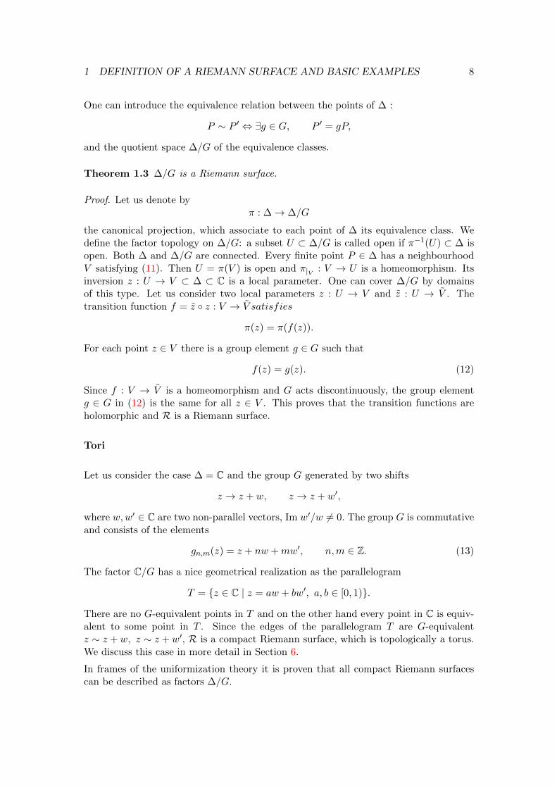
The factor ℂ/G has a nice geometrical realization as the parallelogram

T = {z ∈ ℂ ∣ z = aw + bw′, a, b ∈ [0, 1)}.

There are no G-equivalent points in T and on the other hand every point in ℂ is equiv-alent to some point in T . Since the edges of the parallelogram T are G-equivalentz ∼ z +w, z ∼ z +w′, ℛ is a compact Riemann surface, which is topologically a torus.We discuss this case in more detail in Section 6.

In frames of the uniformization theory it is proven that all compact Riemann surfacescan be described as factors Δ/G.


w0

w′ w + w′

Figure 2: A complex torus

1.3 Euclidean Polyhedral Surfaces as Riemann Surfaces

It is not difficult to build a Riemann surface glueing together pieces of the complex planeℂ.

Consider a finite set of disjoint Euclidean triangles Fi and identify their elements (verticesand edges) is such a way that they comprise a compact oriented Euclidean polyhedralsurface. A polyheder in 3-dimensional Euclidean space is an example of such a surface.A required identification of edges and vertices is shown in Fig. 3. It is characterized bythe following properties.

(i) If two triangles have common elements then these may be either a common vertex ora common edge.

(ii) Every edge of the surface belongs exactly to two triangles.

(iii) Triangles with a common vertex P are successively glued along edges passing throughP (as in Fig. 3), i.e. the triangles with a common vertex P are arranged in a cyclicsequence F1, F2, . . . , Fn such that each pair Fi, Fi+1 as well as Fn, F1 has a common edgecontaining P .

(iv) All triangles can be oriented so that their orientations correspond.

In order to define a complex structure on an Euclidean polyhedral surface let us distin-guish three kinds of points:

1. inner points of triangles,

2. inner points of edges,

3. vertices.

�2

�1

�n

Figure 3: Three kinds of points on an Euclidean polyhedral surface


It is clear how to define local parameters for the points of the first and the secondkind. By an Euclidean isometry one can map the corresponding triangles (or pairs ofneighbouring triangles) into ℂ. This provides us with local parameters at the points ofthe first and the second kind. Next let P be a vertex and Fi, . . . , Fn the sequence ofsuccessive triangles with this vertex (see the point (iii) above). Denote by �i the angleof Fi at P . Then define

=2�∑ni=1 �i

.

Consider a suitably small ball neighbourhood of P, which is the union U r = ∪iF ri , whereF ri = {Q ∈ Fi ∣ ∣ Q − P ∣< r}. Each F ri is a sector with angle �i at P . We map it asabove into ℂ with P mapped to the origin and then apply z 7→ z , which produces asector with the angle �i. The mappings corresponding to different triangles Fi can beadjusted to provide a homeomorphism of U r onto a disc in ℂ.

All transition functions of the constructed charts are holomorphic since they are com-positions of maps of the form z 7→ az + b and z 7→ z (away from the origin).

Using the algebraic curve representation of compact Riemann surfaces it is not diffi-cult to show that any compact Riemann surface can be recovered from some Euclideanpolyhedral surface [Bost].

1.4 Complex Structure Generated by Metric

There is a smooth version of the previous construction. Let (ℛ, g) be a two-real dimen-sional orientable differential manifold with a metric g. In local coordinate (x, y) : U ⊂ℛ → ℝ2 one has

g = a dx2 + 2b dxdy + c dy2, a > 0, c > 0, ac− b2 > 0. (14)

Definition 1.5 Two metrics g and g are called conformally equivalent if they differ bya function on ℛ

g ∼ g ⇔ g = fg, f : ℛ → ℝ+. (15)

The relation (15) defines the classes of conformally equivalent metrics.

Remark The angles between tangent vectors are the same for conformally equivalentmetrics.

We show that there is one to one correspendence between the conformal equivalenceclasses of metrics on an orientable two-manifold ℛ and the complex structures on ℛ. Interms of the complex variable3 z = x+ iy one rewrites the metric as

g = Adz2 + 2Bdzdz + Adz2, A ∈ ℂ, B ∈ ℝ, B > ∣A∣, (16)

witha = 2B +A+ A, b = i(A− A), c = 2B −A− A. (17)

3Note that the complex coordinate z is not compatible with the complex structure we will define onℛ with the help of g.


Definition 1.6 A coordinate w : U → ℂ is called conformal if the metric in this coor-dinate is of the form

g = e�dwdw, (18)

i.e. it is conformally equivalent to the standard metric of ℝ2 = ℂ

dwdw = du2 + dv2, w = u+ iv.

Remark If F : U ⊂ ℝ2 → ℝ3 is an immersed surface in ℝ3 then the first fundamentalform < dF, dF > induces a metric on U . When the standard coordinate (x, y) of ℝ2 ⊃ Uis conformal, the parameter lines

F (x,Δm), F (Δn, y), x, y ∈ ℝ, n,m ∈ ℤ, Δ→ 0

comprise an infinitesimal square net on the surface. The problem of conformal coor-dinates was studied already by Gauss, who proved their existence in the real-analyticcase.

We start with a simple

Theorem 1.4 Every compact Riemann surface admits a conformal Riemannian metric.

Proof. Each point P ∈ ℛ possesses a local parameter zP : UP → DP ⊂ ℂ, where DP isa small open disc. Since ℛ is compact there exists a finite covering ∪ni=1UPi = ℛ. Foreach i choose a smooth function mi : DPi → ℝ with

mi > 0 on Di, mi = 0 on ℂ ∖Di.

mi(zPi)dzPi dzPi is a conformal metric on UPi . The sum of these metrics over i = 1, . . . , nyields a conformal metric on ℛ.

Let us show how one finds conformal coordinates. The metric (16) can be written asfollows (we suppose A ∕= 0 )

g = s(dz + �dz)(dz + �dz), s > 0, (19)

where

� =A

2B(1 + ∣�∣2), s =

2B

1 + ∣�∣2.

Here ∣�∣ is a solution of the quadratic equation

∣�∣+ 1

∣�∣=

2B

∣A∣,

which can be chosen ∣�∣ < 1

∣�∣ = 1

∣A∣(B −

√B2 − ∣A∣2). (20)


Comparing (19) and (18) we get

dw = �(dz + �dz)

ordw = �(dz + �dz).

In the first case the map w(z, z) satisfies the equation

wz = �wz (21)

and preserves the orientation w : U ⊂ ℂ → V ⊂ ℂ since ∣�∣ < 1 : for the map z → wwritten in terms of the real coordinates

z = x+ iy, w = u+ iv

one hasdu ∧ dv = ∣wz∣2(1− ∣�∣2)dx ∧ dy.

In the second case w : U → V inverses the orientation.

Definition 1.7 Equation (21) is called the Beltrami equation and �(z, z) is called theBeltrami coefficient.

Let us postpone for a moment the discussion of the proof of existence of solutions tothe Beltrami equation and let us assume that this equation can be solved in a smallneighbourhood of any point of ℛ.

Theorem 1.5 Let ℛ be a two-dimensional orientable manifold with a metric g and anoriented atlas ((x�, y�) : U� → ℝ2)�∈A on ℛ. Let (x, y) : U ⊂ ℛ → ℝ2 be one ofthese coordinate charts with a point P ∈ U, z = x+ iy, �(z, z) - the Beltrami coefficient(20) and w�(z, z) be a solution to the Beltrami equation (21) in a neighbourhood V� ⊂V = z(U) with P ∈ U� = z−1(V�). Then the coordinate w� is conformal and the atlas(w� : U� → ℂ)�∈B defines a complex structure on ℛ.

Proof. To prove the holomorphicity of the transition function let us consider two localparameters w : U → ℂ, w : U → ℂ with a non-empty intersection U ∩ U ∕= ∅. Bothcoordinates are conformal

g = e�dwdw = e�dwd ¯w,

which happens in one of the two cases

∂w

∂w= 0 or

∂w

∂w= 0 (22)

only. The transition function w(w) is holomorphic and not antiholomorphic since themap w → w preserves orientation.

Repearting the arguments of the proof of Theorem 1.5 one immeadeately observes thatconformaly equivalent metrics generate the same complex structure. Finally, we obtainthe following


Theorem 1.6 Conformal equivalence classes of metrics on an orientable two-manifoldℛ are in one to one correspondence with the complex structures on ℛ.

On Solution to the Beltrami Equation

For the real-analytic case � ∈ C! the existence of the solution to the Beltrami equationwas known already to Gauss. It can be proven using the Cauchy-Kowalewski theorem.

Theorem 1.7 (Cauchy-Kowalewski)Let

∂mui∂xm0

= Fi(x0, x, u,∂m0+...+mn

∂xm00 . . . ∂xmnn

u),

i = 1, . . . , k, x ∈ ℝn,n∑j=0

mj ≤ m, m0 < m, m ≥ 1,

be a system of k partial differential equations for k functions u1(x, x0), . . . , uk(x, x0).The Cauchy problem

∂jui

∂xj0

∣∣∣∣�

= �ij(x), i = 1, . . . , k; j = 0, . . . ,m− 1,

where � = {(x, x0), x0 = 0, x ∈ Ω0, Ω0 is a domain in ℝn} with real-analytic data(all Fi, �ij are real-analytic functions of all their arguments), has a unique real-analyticsolution u(x, x0) in some domain Ω ⊂ ℝn+1 of variables (x, x0) with Ω0 ⊂ Ω.

In terms of real variables

z = x+ iy, w = u+ iv, � = p+ iq

the Beltrami equation reads as follows:(u

v

)y

=1

(1 + p)2 + q2

(2q p2 + q2 − 1

1− p2 − q2 2q

)(u

v

)x

. (23)

If � is real-analytic and ∣�∣ < 1 all the coefficients in (23) are real-analytic, which impliesthe existence of a real-analytic solution to the equation.

Solutions to the Beltrami equation exist in much more general case but the proof is muchmore involved.

Recall that a function is of Holder class of order � (0 < � < 1) on W , f ∈ C�(W ) ifthere exists a constant K such that

∣f(p)− f(q)∣ ≤ K∣p− q∣�, ∀p, q ∈W.

If all mixed n-th order derivatives of f exist and are C� then f ∈ Cn+�(W ).

Theorem 1.8 Let z : U → V ⊂ ℂ be a coordinate chart at some point P ∈ U and � ∈C�(V ) be the Beltrami coefficient. There is a solution w(z, z) to the Beltrami equationof the class w ∈ C�+1(W ) in some neighbourhood W of the point z(P ) ∈W ⊂ V .


Sketch of the proof of Theorem 1.8.

The Beltrami equation can be rewritten as an integral equation using

Lemma 1.9 (∂-Lemma)Given g ∈ C�(V ), the formula

f(z) =1

2�i

∫V

g(�)

� − zd� ∧ d�

defines a C�+1(V ) solution to the equation

fz(z) = g(z).

In case g ∈ C∞ or g ∈ C1 this lemma is a standard result in complex analysis. For theproof in the case formulated above see [Bers] and [Spivak], v.4.

The ∂-Lemma implies that the solution of

w(z) = ℎ(z) +1

2�i

∫V

�(�)w�(�)

� − zd� ∧ d�, (24)

where ℎ is holomorph, satisfies the Beltrami equation. The proof of the existence ofthe solution to the integral equation (24) is standard: it is solved by iterations. Let usrewrite the equation to be solved as

w = Tw, (25)

where Tw is the right-hand side of (24). Let us suppose that there complete metricspace ℋ such that

i) Tℋ ⊂ ℋ

ii) T is a contraction in ℋ, i. e. ∥Tw − Tw′∥ < c∥w − w′∥ for any w,w′ ∈ ℋ withsome c < 1.

Then there exists a unique solution w∗ ∈ ℋ of (25) and this solution can be obtainedfrom any starting point w0 ∈ ℋ by iteration

w∗ = limn→∞

Tnw0.

For the choice of the function space ℋ and details of the proof see [Bers] and [Spivak],v.4.

The theorem above holds true also after replacing �→ �+ n, n ∈ ℕ.

2 HOLOMORPHIC MAPPINGS 15

2 Holomorphic Mappings

Definition 2.1 A mappingf : M → N

between Riemann surfaces is called holomorphic (or analytic) if for every local parameter(U, z) on M and every local parameter (V,w) on N with U ∩ f−1(V ) ∕= ∅, the mapping

w ∘ f ∘ z−1 : z(U ∩ f−1(V ))→ w(V )

is holomorphic.

A holomorphic mapping into ℂ is called a holomorphic function, a holomorphic mappinginto ℂ is called a meromorphic function.

The following lemma characterizes a local behaviour of holomorphic mappings.

Lemma 2.1 Let f : M → N be a holomorphic mapping. Then for any a ∈ M thereexist local parameters (U, z), (V,w) such that a ∈ U, f(a) ∈ V and F = w ∘ f ∘ z−1 :z(U)→ w(V ) equals

F (z) = zk, k ∈ ℕ. (26)

Proof Let us normalize local parameters z near a and w near f(a) to vanish at thesepoints: z(a) = w(f(a)) = 0. Since F (z) is holomorphic and F (0) = 0 it can be rep-resenred as F (z) = zkg(z), where g(z) is holomorphic and g(0) ∕= 0. The map z → zwith

z = zℎ(z), ℎk(z) = g(z)

is biholomorphic and in terms of the local parameter z the mapping w ∘ f ∘ z−1 is givenby (26).

Corollary 2.2 Let f : M → N be a non-constant holomorphic mapping, then f is open,i.e. an image of any open set is open.

Corollary 2.3 Let f : M → N be a non-constant holomorphic mapping and M com-pact. Then f is surjective f(M) = N and N is also compact.

Proof The previous corollary implies that f(M) is open. On the other hand, f(M)is compact since it is a continuous image of a compact set. f(M) is open, closed andnon-empty, therefore f(M) = N and N compact.

Theorem 2.4 (Liouville)There are no non-constant holomorphic functions on compact Riemann surfaces.


Proof An existence of a non-constant holomorphic mapping f : M → ℂ contradicts tothe previous corollary since ℂ is not compact.

Non-constant holomorphic mappings of Riemann surfaces f : M → N are discrete: forany point P ∈ N the set SP = f−1(P ) is discrete, i.e. for any point a ∈ M thereis a neighbourhood V ⊂ M intersecting with SP in at most one point, ∣V ∩ SP ∣ ≤ 1.Non-discreteness of S for a holomorphic mapping would imply the existence of a limitingpoint in SP and finally f = const, f : M → P ∈ N. Non-constant holomorphic mappingsof Riemann surfaces are also called holomorphic coverings.

Definition 2.2 Let f : M → N be a holomorphic covering. A point P ∈ M is called abranch point of f if it has no neighbourhood V ∋ P such that f

∣∣V

is injective. A coveringwithout branch points is called unramified (ramified or branched covering in the oppositecase).4

The number k ∈ ℕ in Lemma 2.1 can be described in topological terms. There existneighbourhoods U ∋ a, V ∋ f(a) such that for any Q ∈ V ∖{f(a)} the set f−1(Q) ∩ Uconsists of k points. One says that f has the multiplicity k at a. Lemma 2.1 allows us tocharacterize the branch points of a holomorphic covering f : M → N as the points withthe multiplicity k > 1. Equivalently, P is a branch point of the covering f : M → N if

∂(w ∘ f ∘ z−1)

∂z

∣∣∣∣z(P )

= 0, (27)

where z and w are local parameters at P and f(P ) respectively (due to the chain rule thiscondition is independent of the choice of the local parameters). The number bf (P ) = k−1is called the branch number of f at P ∈ M. The next lemma also immediately followsfrom Lemma 2.1.

Lemma 2.5 Let f : M → N be a holomorphic covering. Then the set of branch points

B = {P ∈M ∣ bf (P ) > 0}

is discrete. If M is compact, then B is finite.

Proof Let P ∈ M . Then exists U ∋ P , such that F (z) := (w ∘ f ∘ z−1)(z) = zk on U ,where k = bf + 1. Since the map zk is locally injective for all z ∕= 0, the point P is theonly possible branch point in U .

Now, if you suppose B to be infinite, this contradicts the discreteness of B, because aninfinite subset in a compact set M has a limiting point P ∈M and therefore there wouldbe infinitely many points with bf > 0 in any neighbourhood of P .

4Note that there are various definitions of a covering of manifolds used in the literature (see forexample [Bers, Jost, Beardon]). In particular often the term ”covering” is used for unramified coveringsof our definition. Ramified coverings are important in the theory of Riemann surfaces.


b = 2

b = 1b = 1

N

f

M

Figure 4: Covering

Theorem 2.6 Let f : M → N be a non-constant holomorphic mapping between twocompact Riemann surfaces. Then there exists m ∈ ℕ such that every Q ∈ N is assumedby f precisely m times - counting multiplicities; that is for all Q ∈ N∑

P∈f−1(Q)

(bf (P ) + 1) = m. (28)

Proof The set of branch points B is finite, therefore its projection A = f(B) is alsofinite. Any two points Q1, Q2 ∈ N∖A can be connected by a curve l ⊂ N∖A. Sincef−1(l) ∩ B = ∅, the map f is a homeomorphism near each component of f−1(l), andf−1(l) consists of m non-intersecting curves l1, . . . , lm (m is finite, otherwise the setf−1(Q1) has a limiting point and f is constant). This shows that the number of preimagesfor any points in N∖A is the same.

Generally (see Fig. 4), for a point Q ∈ N there are n preimages P1, . . . , Pn with f(Pi) =Q and the corresponding branch numbers b(Pi). These points have non-intersectingneighbourhoods U1, . . . , Un, Pi ∈ Ui, �(Ui) = U ∀i, Ui ∩ Uj = ∅ such that for anyQ ∈ U∖{Q} there are exactly b(Pi) + 1 points of f−1(Q) lying in Ui. Since Q ∈ N∖Athe previous consideration implies (28).

Definition 2.3 The number m above is called the degree of f . The covering f : M → Nis called m-sheeted.

Applying Theorem 2.6 to holomorphic mappings f : ℛ → ℂ we get

Corollary 2.7 A non-constant meromorphic function on a compact Riemann surfaceassumes every its value in ℂ m times, where m is the number of its poles (countingmultiplicities).

Remark A single non-constant meromorphic function f : ℛ → ℂ completely determinesthe complex structure of the Riemann surface. A local parameter vanishing at P0 ∈ ℛis given by

(f(P )− f(P0))1/k(P0) for f(P0) ∕=∞,where k(P0) = bf (P0) + 1. For f(P0) = ∞ one uses the local coordinate 1/z for a

neighbourhood of ∞ in ℂ, and a local parameter is given by

(f(P ))−1/k(P0) for f(P0) =∞.


0

Figure 5: Riemann surface of√�

2.1 Algebraic curves as coverings

Let C be a non-singular algebraic curve (1) and C its compatification. The mapping

(�, �)→ � (29)

defines a holomorphic covering C → ℂ. If N is the degree of the polynomial P(�, �) in�

P(�, �) = �NpN (�) + �N−1pN−1(�) + . . .+ p0(�),

where all pi(�) are polynomials, then � : C → ℂ is an N -sheeted covering.

The points with ∂P/∂� = 0 are the branch points of the covering � : C → ℂ. Indeed,at these points ∂P/∂� ∕= 0, and � is a local parameter. The derivative of � with respectto the local parameter vanishes

∂�

∂�= −∂P/∂�

∂P/∂�= 0,

which characterizes (27) the branch points of the covering (29). In the same way Ccovers (�, �) → � the complex plane of �. The branch points of this covering are thepoints with ∂P/∂� = 0.

Hyperelliptic curves

Considering the hyperelliptic case let us remind a conventional description of the Rie-mann surface of the function � =

√� from the basic course of complex analysis. One

imagines oneself two copies of the complex plane ℂ with a cut [0,∞] glued together cross-wise along this cut (see Fig. 5). The image in Fig. 5 is in one to one correspondencewith the points of the curve

C = {(�, �) ∈ ℂ2 ∣ �2 = �},

and the point � = 0 gives an idea of a branch point.

The compactification C of the hyperelliptic curve

C = {(�, �) ∈ ℂ2 ∣ �2 =N∏i=1

(�− �i)} (30)


ℂ ℂ

Figure 6: Topological image of a hyperelliptic surface

�6�1

�2

�5

�4�3

Figure 7: Hyperelliptic surface C as a two-sheeted cover. The parts of the curves on Cthat lie on the second sheet are indicated by dotted lines.

is a two sheeted covering of the extended complex plane � : C → ℂ. The branch pointsof this covering are

(0, �i), i = 1, . . . , N and ∞ for N = 2g + 1,

(0, �i), i = 1, . . . , N for N = 2g + 2,

with the branch numbers b� = 1 at these points. Only the branching at � =∞ possiblyneeds some clarification. The local parameter at ∞ ∈ ℂ is 1/�, whereas the localparameter at the point ∞ ∈ C of the curve C with N = 2g + 1 is 1/

√� due to (9). In

these coordinates the covering mapping reads as (compare with (26))

1

�=

(1√�

)2

,

which shows that b�(∞) = 1.

One can imagine oneself the Riemann surface C with N = 2g+2 as two Riemann sphereswith the cuts

[�1, �2], [�3, �4], . . . , [�2g+1, �2g+2]

glued together crosswise along the cuts. Fig. 6 presents a topological image of thisRiemann surface. Later on we will use the image shown in Fig. 7, where we see theRiemann surface ”from above” or ”the first” sheet on the covering � : C → ℂ and shouldadd the points at infinity to this image. In the case N = 2g + 1 one should move thebranch point �2g+2 to infinity.

The hyperelliptic curves obey a holomorphic involution

ℎ : (�, �)→ (−�, �), (31)


Figure 8: Two equivalent images of a hyperelliptic Riemann surface

which interchanges the sheets of the covering � : C → ℂ and is called hyperelliptic. Thebranch points of the covering are the fixed points of ℎ.

Remark The cuts in Fig. 7 are conventional and belong to the image shown in Fig. 7and not to the hyperelliptic Riemann surface itself, which is determined by its branchpoints. In particular, the images shown in Fig.8 correspond to the same Riemann surfaceand to the same covering (�, �)→ �.

2.2 Quotients of Riemann Surfaces as Coverings

In Section 1.2 we defined the complex structure on the factor Δ/G, where Δ is a domainin ℂ, so that the canonical projection

� : Δ→ Δ/G

is holomorphic. This construction can be also applied to Riemann surfaces.

Theorem 2.8 Let ℛ be a (compact) Riemann surface and G a finite group of its holo-morphic automorphisms5 of order ordG. Then ℛ/G is a Riemann surface with thecomplex structure determined by the condition that the canonical projection

� : ℛ → ℛ/G

is holomorphic. This is an ordG-sheeted covering, ramified at fixed points of G.

Proof The consideration for the case when P ∈ ℛ is not a fixed point of G (there arefinitely many fixed points of G) is the same as for Δ/G above. The canonical projection� defines an ordG-sheeted covering unramified at these points. Let P0 be a fixed pointand denote by

GP0 = {g ∈ G ∣ gP0 = P0}

the stabilizer of P0. It is always possible to choose a neighborhood U of P0 with noother fixed point than P0 in U , which is invariant with respect to all elements of GP0

and such that U ∩ gU = ∅ for all g ∈ G ∖ GP0 . Let us normalize the local parameter zon U by z(P0) = 0. The local parameter w in �(U), which is ordGP0-sheetedly coveredby U is defined by the product of the values of the local parameter z at all equivalentpoints lying in U . In terms of the local parameter z all the elements of the stabilizerare represented by the functions g = z ∘ g ∘ z−1 : z(U) → z(U), which vanish at z = 0.

5We will see later that this group is always finite if the genus ≥ 2.


Since g(z) are also invertible they can be represented as g(z) = zℎg(z) with ℎg(0) ∕= 0.Finally the w − z coordinate charts representation of �

w ∘ � ∘ z−1 : z → zordGP0∏

g∈GP0

ℎg(z)

shows that the branch number of P0 is ordGP0 .

The compact Riemann surface C of the hyperelliptic curve

�2 =

2N∏n=1

(�2 − �2n), �2

i ∕= �2j , �k ∕= 0 (32)

has the following group of holomorphic automorphisms

ℎ : (�, �)→ (−�, �)

i1 : (�, �)→ (�,−�)

i2 = ℎi1 : (�, �)→ (−�,−�).

The hyperelliptic involution ℎ interchanges the sheets of the covering � : C → ℂ, there-fore the factor C/ℎ is the Riemann sphere. The covering

C → C/ℎ = ℂ

is ramified at all the points � = ±�n.

The involution i1 has four fixed points on C: two points with � = 0 and two points with� =∞. The covering

C → C1 = C/i1 (33)

is ramified at these points. The mapping (33) is given by

(�, �)→ (�,Λ), Λ = �2,

and C1 is the Riemann surface of the curve

�2 =2N∏n=1

(Λ− �2n).

The involution i2 has no fixed points. The covering

C → C2 = C/i2 (34)

is unramified. The mapping (34) is given by

(�, �)→ (M,Λ), M = ��, Λ = �2,

and C2 is the Riemann surface of the curve

M2 = Λ

2N∏n=1

(Λ− �2n).

3 TOPOLOGY OF RIEMANN SURFACES 22

3 Topology of Riemann Surfaces

3.1 Spheres with Handles

We have seen in Section 1 that any Riemann surface is a two-real-dimensional orientablesmooth manifold. In this section we present basic facts about topology of these mani-folds focusing on the compact case. We start with an intuitively natural fundamentalclassification theorem and comment its proof later on.

Theorem 3.1 (and Definition) Any compact Riemann surface is homeomorphic toa sphere with handles 6. The number g ∈ ℕ of handles is called the genus of ℛ. Twomanifolds with different genera are not homeomorphic.

b2

b1

a2

a1

Figure 9: Sphere with 2 handles

The genus of the compactification C of the hyperelliptic curve (30) with N = 2g + 1 orN = 2g + 2 is equal to g.

For many purposes it is convenient to use planar images of spheres with handles.

Proposition 3.2 Let Πg be an extended plane7 with 2g holes bounded by the non-intersecting curves

1, ′1, . . . , g,

′g. (35)

and the curves i ≈ ′i, i = 1, . . . , g are topologically identified in such a way that theorientations of these curves with respect to Πg are opposite (see Fig. 10). Then Πg ishomeomorphic to a sphere with g handles.

1

g ′g

′1

Πg

Figure 10: Planar image of a sphere with g handles

6By a sphere with handles we mean a topological manifold homeomorphic to a sphere with handlesin Euclidean 3-space.

7By an extended plane we mean ℝ2 ∪ {∞}, which is homeomorphic to S2.


To prove this proposition one should cut up all the handles of a sphere with g handles.

A normalized simply-connected image of a sphere with g handles is described by thefollowing proposition.

Proposition 3.3 Let Fg be a 4g-gon with the edges

a1, b1, a′1, b′1, . . . , ag, bg, a

′g, b′g, (36)

listed in the order of traversing the boundary of Fg and the curves

ai ≈ a′i, bi ≈ b′i, i = 1, . . . , g

are topologically identified in such a way that the orientations of the edges ai and a′i aswell as bi and b′i with respect to Fg are opposite (see Fig. 11). Then Fg is homeomorphicto a sphere with g handles. The sphere without handles (g = 0) is homeomorphic to the2-gon with the edges

a, a′, (37)

identified as above.

b′1

b1

b′g

a′1

a1

a′g

ag

Fgbg

Figure 11: Simply-connected image of a sphere with g handles

Proof is given in Figs. 12, 13. One choice of closed curves a1, b1, . . . , ag, bg on a spherewith handles is shown in Fig. 9.

a

b≃ ≃b

a

a′

b′a

b′

b

Figure 12: Gluing a torus

Let us consider a triangulation T of ℛ, i.e. a set {Ti} of topological triangles on ℛ,which cover ℛ

∪Ti = ℛand the intersection Ti∩Tj for any Ti, Tj is either empty or consists of one common edgeor of one common vertex (compare with Section 1.3). Obviously, compact Riemannsurfaces are triangularizable by finite triangulations8.

8Due to Rado’s theorem (see for example [AlforsSario]) any Riemann surface is triangularizable.


∼=∼= ∼=a

lb

a′

b′

l

a

a′

b alb′

b

a

b

Figure 13: Gluing a handle

Definition 3.1 Let T be a triangulation of a compact two-real dimensional manifold ℛand F be the number of triangles, E - the number of edges, V - the number of verticesof T . The number

� = F − E + V (38)

is called the Euler characteristics of ℛ.

Proposition 3.4 The Euler characteristic �(ℛ) of a compact Riemann surface9 ℛ isindependent of the triangulation of ℛ.

Proof. Introduce a conformal metric eu dzdz on a Riemann surface (Theorem 1.4). TheGauss–Bonnet theorem provides us with the following formula for the Euler characteristic

�(ℛ) =1

2�

∫ℛK, (39)

whereK = −2uzze

−u

is the curvature of the metric. The right hand side in (39) is independent of the triangu-lation, the left hand side is independent of the metric we introduced on ℛ. This provesthat the Euler characteristics is a topological invariant of ℛ.

Corollary 3.5 The Euler characteristics �(ℛ) of a compact Riemann surface ℛ ofgenus g is equal

�(ℛ) = 2− 2g. (40)

For the proof of this corollary it is convenient to consider the simply-connected modelFg of Proposition 3.3.

Sketch of the proof of Theorem 3.1. Let ℛ be a compact Riemann surface and T atriangulation of ℛ oriented in accordance with the orientation of ℛ. Each triangle Tican be mapped onto an Euclidean triangle. Successively mapping neighboring triangleswe finally obtain a n+ 2-gon, where n is the number of triangles in T . Since each side ofthis polygon is identified with precisely one other side, the polygon has an even number

9The statement of the Proposition holds true also for general two-real dimensional manifolds. Theproof is combinatorial.


of edges. Let us label the edges of this polygon, labelling one of the identified edgesby c and the other by c′. We call the word obtained by writing the letters in orderof traversing the boundary the symbol of the polygon. By cutting up the polygon andpasting it after that in another way one can simplify the symbol. The simplificationto the normal form (35) (g > 0) or (36) (g = 0) can be described explicitly. All thedetails of this process can be found for example in [Springer, Bers]. We see that ℛ ishomeomorphic to Fg with some g. In its turn, due to Proposition 3.3 Fg is obviouslyhomeomorphic to a sphere with g handles.

Directly from Definition 3.1 one gets that the Euler characteristics of two homeomorphicmanifolds coincide. This implies that Fg and Fg are homeomorphic if and only if g = g,which completes the proof.

Theorem 3.6 (Riemann-Hurwitz)Let f : ℛ → ℛ be an N -sheeted covering of compact Riemann surfaces and ℛ is of genusg. Then the genus g of ℛ is given by

g = N(g − 1) + 1 +b

2, (41)

whereb =

∑P∈ℛ

bf (P ) (42)

is the total branching number.

Proof As it was shown in Lemma 2.5 the set B = {P ∈ ℛ ∣ bf (P ) > 0} is finite. Wetriangulate ℛ so that every point of A = f(B) ⊂ ℛ is a vertex of the triangulation.Let us assume that the triangulation has F faces, E edges and V vertices. Then theinduced triangulation lifted to ℛ via the mapping f has NF faces, NE edges and NV −bvertices, where b is given by (42). For the Euler characteristics of ℛ and ℛ this implies

�(ℛ) = N�(ℛ)− b,

which is equivalent to (41) because of (38).

3.2 Fundamental group

Let P and Q be two points on ℛ and PQ a curve, i.e. a continuous map : [0, 1]→ ℛ,connecting them PQ(0) = P, PQ(1) = Q.

Definition 3.2 Two curves 1PQ,

2PQ on ℛ with the initial point P and the termi-

nal point Q are called homotopic if they can be continuously deformed one to another,i.e. provided there is a continuous map : [0, 1] × [0, 1] → ℛ such that (t, 0) = 1PQ(t), (t, 1) = 2

PQ(t), (0, �) = P, (1, �) = Q. The set of homotopic curves formsa homotopic class, which we denote by ΓPQ = [ PQ].


If the terminal point of 1 coincides with the initial point of 2 the curves can bemultiplied:

1 ⋅ 2(t) =

{ 1(2t) 0 ≤ t ≤ 1

2 2(2t− 1) 1

2 ≤ t ≤ 1.

This multiplication is well-defined also for the corresponding homotopic classes

Γ1 ⋅ Γ2 = [ 1 ⋅ 2].

Any two closed curves through P can be multiplied. The set of homotopic classes ofthese curves forms a group �1(ℛ, P ) with the multiplication defined above. The curves,which can be contracted to a point correspond to the identity element of the group.It is easy to see that the groups �1(ℛ, P ) and �1(ℛ, Q) based at different points areisomorphic as groups. Considering this group one can omit the second argument in thenotation

�1(ℛ, P ) ≈ �1(ℛ, Q) ≈ �1(ℛ).

Definition 3.3 The group �1(ℛ) is called the fundamental group of ℛ.

Examples

1. Sphere with N holes

D1

2D2DN

N

1

Figure 14: Fundamental group of a sphere with N holes

ℛ = S ∖ {∪Nn=1Dn}.

The fundamental group is generated by the homotopic classes of the closed curves 1, . . . , N each going around one of the holes (Fig 14). The curve 1 2 . . . N can becontracted to a point, which implies the relation

Γ1Γ2 . . .ΓN = 1 (43)

in �1(S ∖ {∪Nn=1Dn}).

2. Compact Riemann surface of genus g.


a1

b1

a−11

b−11

ag

bg

b−1g

a−1g

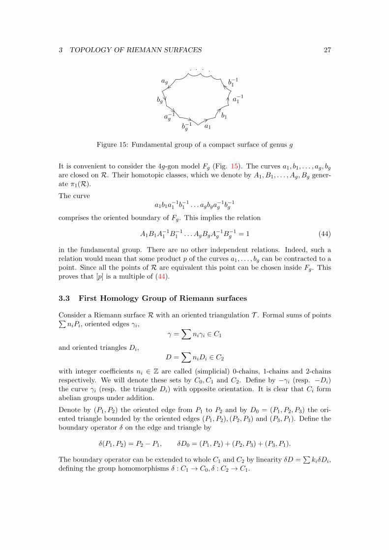
Figure 15: Fundamental group of a compact surface of genus g

It is convenient to consider the 4g-gon model Fg (Fig. 15). The curves a1, b1, . . . , ag, bgare closed on ℛ. Their homotopic classes, which we denote by A1, B1, . . . , Ag, Bg gener-ate �1(ℛ).

The curvea1b1a

−11 b−1

1 . . . agbga−1g b−1

g

comprises the oriented boundary of Fg. This implies the relation

A1B1A−11 B−1

1 . . . AgBgA−1g B−1

g = 1 (44)

in the fundamental group. There are no other independent relations. Indeed, such arelation would mean that some product p of the curves a1, . . . , bg can be contracted to apoint. Since all the points of ℛ are equivalent this point can be chosen inside Fg. Thisproves that [p] is a multiple of (44).

3.3 First Homology Group of Riemann surfaces

Consider a Riemann surface ℛ with an oriented triangulation T . Formal sums of points∑niPi, oriented edges i,

=∑

ni i ∈ C1

and oriented triangles Di,

D =∑

niDi ∈ C2

with integer coefficients ni ∈ ℤ are called (simplicial) 0-chains, 1-chains and 2-chainsrespectively. We will denote these sets by C0, C1 and C2. Define by − i (resp. −Di)the curve i (resp. the triangle Di) with opposite orientation. It is clear that Ci formabelian groups under addition.

Denote by (P1, P2) the oriented edge from P1 to P2 and by D0 = (P1, P2, P3) the ori-ented triangle bounded by the oriented edges (P1, P2), (P2, P3) and (P3, P1). Define theboundary operator � on the edge and triangle by

�(P1, P2) = P2 − P1, �D0 = (P1, P2) + (P2, P3) + (P3, P1).

The boundary operator can be extended to whole C1 and C2 by linearity �D =∑ki�Di,

defining the group homomorphisms � : C1 → C0, � : C2 → C1.


C1 contains two important subgroups - of cycles and of boundaries. A 1-chain with� = 0 is called a cycle, a 1-chain = �D is called a boundary. We denote thesesubgroups by

Z = { ∈ C1 ∣ � = 0}, B = �C2.

Due to �2 = 0 every boundary is a cycle and we have B ⊂ Z ⊂ C1.

One can introduce an equivalence relation between elements of C1. Two 1-chains arecalled homologous if their difference is a boundary:

1 ∼ 2, 1, 2 ∈ C1 ⇔ 1 − 2 ∈ B, i.e. ∃D ∈ C2 : �D = 1 − 2.

Definition 3.4 The factorgroup

H1(ℛ,ℤ) = Z/B

is called the first homology group of ℛ.

All the groups we consider are abelian and the elements of H1(ℛ,ℤ) can be describedas equivalence classes10

[ ] ∈ {1− cycles}{1− dimensional boundaries}

.

Any closed oriented continuous curve (i.e. periodic continuous map : [0, 1] → ℛ)can be deformed homotopically into a 1-cycle in the triangulation T . To show thisone should consider the triangles of T close to and construct the 1-cycle using theedges of their boundaries. Details of this construction can be found in [Springer]. Sincehomotopical simplicial 1-cycles are obviously homologous, this insight allows us to definethe homology group as a homology group of cycles composed of arbitrary closed curvesrather than symplicial 1-cycles on ℛ. We call such a curve a simple cycle on ℛ.

This definition of homologous continuous cycles later will be shown to be independentof T . Directly from the definition follows that freely homotopic closed curves are ho-mologous. Note that the converse is however false in general as one can see from theexample in Fig. 16.

Figure 16: A cycle homologous to zero but not homotopic to a point.

10Considering n-chains on a triangulated manifold one can analogously define n-th homology group.Homology groups can be also introduced over arbitrary fields if one considers formal linear combinationswith coefficients in these fields. For example so one can define H1(ℛ,ℤ2), Hn(ℛ,ℝ) etc.


The first homology group is the fundamental group ”made commutative”11. Indeed,let be a 1-cycle on ℛ with a point P0 ∈ and Γ1, . . . ,Γn be generators of �(ℛ, P0).Denote by [ ], [Γ1], . . . , [Γn] ∈ H1(ℛ,ℤ) the corresponding homology classes. The cycle is homotopic to

= Γj1i1 . . .Γjkik, i1, . . . , ik ∈ {1, . . . , n}, ji ∈ ℤ,

which implies for the homology classes

[ ] = j1[Γi1 ] + . . . jk[Γik ].

By linearity this representation can be extended to arbitrary combination of cycles inH1(ℛ,ℤ). As in Section 3.2 it is easy to see that [Γi] are independent of P0. Finally we seethat the homology group is the abelian group generated by the elements [Γi], i = 1, . . . , n.This shows in particular that the whole construction is independent of the triangulationT we started with.

To introduce intersection numbers of elements of the first homology group it is convenientto represent them by smooth cycles. Every element of H1(ℛ,ℤ) can be represented by aC∞-cycle. Moreover given two elements of H1(ℛ,ℤ) one can represent them by smoothcycles intersecting transversally in finite number of points.

Let 1 and 2 be two curves intersecting transversally at the point P . One associates tothis point a number ( 1 ∘ 2)P = ±1, where the sign is determined by the orientation ofthe basis ′1(P ), ′2(P ) as it is shown in Fig. 17.

1 2

2 1

( 1 ∘ 2)P = 1

P P

( 1 ∘ 2)P = −1

Figure 17: Intersection number at a point.

Definition 3.5 Let 1, 2 be two smooth cycles intersecting transversally at the finiteset of their intersection points. The intersection number of 1 and 2 is defined by

1 ∘ 2 =∑

P∈Intersection set

( 1 ∘ 2)P . (45)

Lemma 3.7 The intersection number of any boundary � with any cycle vanishes, i.e. ∘ � = 0.

11Precisely

H1(ℛ,ℤ) =�(ℛ)

[�(ℛ), �(ℛ)],

where the denominator is the commutator subgroup, i.e. the subgroup of �(ℛ) generated by all elementsof the form ABA−1B−1, A,B ∈ �(ℛ).


Proof. Since (45) is bilinear it is enough to prove the statement for a boundary of adomain � = �D and a simple cycle . In this case the statement follows from the simplefact that the cycle goes as many times inside D as outside (see Fig. 18).

D

�D

Figure 18: ∘ �D = 0.

To define the intersection number on homologies represent , ′ ∈ H1(ℛ,ℤ) by C∞-cycles

=∑i

ni i, ′ =∑j

mj ′i,

where i, ′j are smooth curves intersecting transversally. Define ∘ ′ =

∑ij nimj i ∘ ′j .

Due to Lemma 3.7 the intersection number is well defined on homologies.

Theorem 3.8 The intersection number is a bilinear skew-symmetric map

∘ : H1(ℛ,ℤ)×H1(ℛ,ℤ)→ ℤ.

Examples

1. Homology group of a sphere with N holes.

The homology group is generated by the loops 1, . . . , N−1 (see Fig. 14). For thehomology class of the loop N one has

N = −N−1∑i=1

i,

since∑N

i=1 i is a boundary.

2. Homology group of a compact Riemann surface of genus g.

Since the homotopy group is generated by the cycles a1, b1, . . . , ag, bg shown in Fig. 15it is also true for the homology group. The intersection numbers of these cycles are asfollows

ai ∘ bj = �ij , ai ∘ aj = bi ∘ bj = 0. (46)

The cycles a1, b1, . . . , ag, bg build a basis of the homology group. They are distinguishedby their intersection numbers and as a consequence are linearly independent.


Definition 3.6 A homology basis a1, b1, . . . , ag, bg of a compact Riemann surface ofgenus g with the intersection numbers (46) is called canonical basis of cycles.

Remark Canonical basis of cycles is by no means unique. Let (a, b) be a canonicalbasis of cycles. We represent it by a 2g-dimensional vector

(ab

), a =

⎛⎜⎝ a1...ag

⎞⎟⎠ , b =

⎛⎜⎝ b1...bg

⎞⎟⎠ .

Any other basis (a, b) of H1(ℛ,ℤ) is then given by the transformation(a

b

)= A

(ab

), A ∈ SL(2g,ℤ). (47)

Substituting (47) into

J =

(a

b

)∘ (a, b), J =

(0 I−I 0

)we obtain that the basis (a, b) is canonical if and only if A is symplectic A ∈ Sp(g,ℤ),i.e.

J = AJAT . (48)

Two examples of canonical basis of cycles are presented in Figs. 19, 20. The curves biin Fig. 19 connect identified points of the boundary curves and therefore are closed. InFig. 20 the parts of the cycles lying on the ”lower” sheet of the covering are marked bydotted lines.

b1a1

ag

bg

Πg

Figure 19: Canonical basis of cycles on the planar model Πg of a compact Riemannsurface.

4 ABELIAN DIFFERENTIALS 32

�2g �2g+2�2 �4 �2g−1 �2g+1�1 �3

b1

b2 bg

a2a1 ag

Figure 20: Canonical basis of cycles of a hyperelliptic Riemann surface.

4 Abelian differentials

Our main goal is to construct functions on compact Riemann surfaces with prescribedanalytical properties (for example, meromorphic functions with prescribed singularities).This and next sections are devoted to this problem. We start with a description ofmeromorphic differentials, which are much simpler to handle than the functions andwhich are the basic tool to investigate and to construct functions.

4.1 Differential forms and integration formulas

We recall the theory of integration on 2-dimensional C∞-manifolds using complex nota-tions. Let ℛ be such a manifold and

z : U ⊂ ℛ → V ⊂ ℂ

be local parameters. The transition functions z(z, z) defined for non-trivial intersectionsU ∩ U

z ∘ z−1 : z(U ∩ U)→ z(U ∩ U) (49)

are C∞.

If to each local coordinate on ℛ there are assigned complex valued functions12

f(z, z), p(z, z), q(z, z), s(z, z) such that

f = f(z, z),

! = p(z, z)dz + q(z, z)dz, (50)

S = s(z, z)dz ∧ dz.

are invariant under coordinate changes (49) one says that the function (0-form) f , thedifferential (1-form) ! and the 2-form S are defined on ℛ. The identification

dz = dx+ idy, dz = dx− idy12We will not treat the problems in the most general setup and assume that the functions are smooth.

It will be enough for applications in the Riemann surface theory.


implies the standard description of !, S in real coordinates x, y. The exterior productof two 1-forms !1 and !2 is the 2-form

!1 ∧ !2 = (p1q2 − p2q1)dz ∧ dz.

If we let !(1,0) = p(z, z)dz, !(0,1) = q(z, z)dz, the forms !(1,0) and !(0,1) are independentof the choice of the local holomorphic coordinate and therefore are differentials definedglobally on ℛ. The 1-form ! is called a form of type (1,0) (resp. a form of type (0,1)) ifflocally it may be written ! = p dz (resp. ! = q dz), i.e. its (0,1)-part (resp. (1,0)-part)vanish. The space of differentials is obviously a direct sum of the subspaces of (1,0) and(0,1) forms.

One can integrate:

1. 0-forms over 0-chains, which are finite sets {P�}� of points P� ∈ ℛ:∑�

f(P�),

2. 1-forms over 1-chains (paths, i.e. smooth oriented curves, and their finite unions):∫

!,

3. 2-forms over 2-chains (finite unions of domains):∫D

S.

Here if : [0, 1]→ U and D ⊂ U are contained in a single coordinate disc, the integralsare defined by

∫

! =

1∫0

(p(z( (t)), z( (t)))

dz( )

dt+ q(z( (t)), z( (t)))

dz( )

dt

)dt,

∫U

S =

∫V

s(z, z)dz ∧ dz.

Due to invariance of (50) under coordinate changes the integrals are well-defined.

The differential operator d, which transforms k-forms into (k + 1)-forms is defined by

df = fzdz + fzdz,

d! = (qz − pz)dz ∧ dz, (51)

dS = 0.


Definition 4.1 A differential df is called exact. A differential ! with d! = 0 is calledclosed.

One can also easily check using (51), that

d2 = 0

whenever d2 is defined andd(f!) = df ∧ ! + fd! (52)

for any function f and 1-form !. This implies in particular that any exact form is closed.

The most important property of d is contained in

Theorem 4.1 (Stokes)Let D be a 2-chain with a piecewise smooth boundary ∂D. Then the Stokes formula∫

D

d! =

∫∂D

! (53)

holds for any differential !.

Our principal interest will be in 1-forms. Let PQ be a curve connecting P and Q. Whendoes the integral

∫ PQ

! depend on the points P,Q and not on the integration path?

Corollary 4.2 A differential ! is closed, d! = 0, if and only if for any two homologicalpaths and ∫

! =

∫

!

holds.

Proof The difference of two homological curves − is a boundary for some D.Applying (53) we have ∫

! −∫

! =

∫∂D

! =

∫D

d! = 0.

The differential ! is closed since D is arbitrary.

Corollary 4.3 Let ! be a closed differential, Fg be a simply connected model of Riemannsurface of genus g (see Section 3) and P0 be some point in Fg. Then the function

f(P ) =

P∫P0

!, P ∈ Fg,

where the integration path lies in Fg is well-defined on Fg.


One can easily check the identity

d(

P∫P0

!) = !(P ). (54)

Let 1, . . . , n be a homology basis of ℛ and ! a closed differential. Periods of ! aredefined by

Λi =

∫ i

!.

Any closed curve on ℛ is homological to∑ni i with some ni ∈ ℤ, which implies∫

! =∑

niΛi,

i.e. Λi generate the lattice of periods of !. In particular, if ℛ is a Riemann surface ofgenus g with the canonical homology basis a1, b1, . . . , ag, bg, we denote the correspondingperiods by

Ai =

∫ai

!, Bi =

∫bi

!.

Theorem 4.4 (Riemann’s bilinear identity)Let ℛ be a Riemann surface of genus g with a canonical basis ai, bi, i = 1, . . . , g andFg be its simply-connected model. Also let ! and !′ be two closed differentials on ℛ andAi, Bi, A

′i, B

′i, i = 1, . . . , g be their periods. Then∫

ℛ

! ∧ !′ =∫∂Fg

!′(P )

P∫P0

! =

g∑j=1

(AjB′j −A′jBj), (55)

where P0 is some point in Fg and the integration path [P0, P ] lies in Fg.

Proof The Riemann surface ℛ cut along all the cycles ai, bi, i = 1, . . . , g of the fun-damental group is the simply connected domain Fg with the boundary (see Figs. 11,15)

∂Fg =

g∑i=1

ai + a−1i + bi + b−1

i . (56)

The first identity in (55) follows directly from the Stokes theorem with D = Fg, Corollary4.3, (52) and (54).

The curves aj and a−1j of the boundary of Fg are identical on ℛ but have opposite

orientation. For the points Pj and P ′j lying on aj and a−1j respectively and coinciding

on ℛ we have (see Fig. 21)

!′(Pj) = !′(P ′j),

Pj∫P0

! −P ′j∫P0

! =Pj∫P ′j

! = −Bj . (57)


In the same way for the points Qj ∈ bj and Q′j ∈ b−1j coinciding on ℛ one gets

!′(Qj) = !′(Q′j),

Qj∫P0

! −Q′j∫P0

! =Qj∫Q′j

! = Aj . (58)

Substituting, we obtain

∫∂Fg

!′(P )

P∫P0

! =

g∑j=1

(−Bj

∫aj

!′ +Aj

∫bj

!′)

=

=

g∑j=1

(AjB′j −A′jBj).

Finally, to prove Riemann’s bilinear identity for an arbitrary canonical basis of H1(ℛ,ℂ)one can directly check that the right hand side of (55) is invariant with respect to thetransformation (47, 48).

Q′j

P ′jQj

Pj

b−1j

a−1j

ajbj

Figure 21: To the proof of the Riemann bilinear relations.

4.2 Abelian differentials of the first, second and third kind

Let now ℛ be a Riemann surface. The transition functions (49) are holomorphic andone can define more special differentials on ℛ.

Definition 4.2 A differential ! on a Riemann surface ℛ is called holomorphic (or anAbelian differential of the first kind) if in any local chart it is represented as

! = ℎ(z)dz

where ℎ(z) is holomorphic. The differential ! is called anti-holomorphic.

Holomorphic and anti-holomorphic differentials are closed.

Holomorphic differentials form a complex vector space, which is denoted by H1(ℛ,ℂ).What is its dimension?


Lemma 4.5 Let ! be a non-zero (! ∕≡ 0) holomorphic differential on ℛ. Then itsperiods Aj , Bj satisfy

Im

g∑j=1

AjBj < 0.

Proof The periods of ! are Aj , Bj . Apply Theorem 4.4 to ! and ! and use

i! ∧ ! = i∣ℎ∣2dz ∧ dz = 2∣ℎ∣2dx ∧ dy > 0.

Corollary 4.6 If all a-periods of the holomorphic differential ! are zero∫aj

! = 0, j = 1, . . . , g,

then ! ≡ 0.

Corollary 4.7 If all periods of a holomorphic differential ! are real, then ! ≡ 0.

Corollary 4.8 dim H1(ℛ,ℂ) ≤ g.

Proof If !1, . . . , !g+1 are holomorphic, then there exists a linear combination of them∑g+1i=1 �i!i with all zero a-periods. Corollary 4.6 implies

∑g+1i=1 �i!i ≡ 0, i.e. the differ-

entials are linearly dependent.

Theorem 4.9 The dimension of the space of holomorphic differentials of a compactRiemann surface is equal to its genus

dim H1(ℛ,ℂ) = g(ℛ).

We give a proof of this theorem in Section 4.4. When the Riemann surface ℛ is con-cretely described, one can usually present the basis !1, . . . , !g of holomorphic differentialsexplicitly.

Theorem 4.10 The differentials

!j =�j−1d�

�, j = 1, . . . , g (59)

form a basis of holomorphic differentials of the hyperelliptic Riemann surface

�2 =

N∏i=1

(�− �i) �i ∕= �j , (60)

where N = 2g + 2 or N = 2g + 1.


Proof The differentials (57) are obviously linearly independent. Their holomorphicityat all the points (�, �) with � ∕= �k, � ∕=∞ is evident. Local parameters at the branchpoints � = �k are zk =

√�− �k. In terms of zk the differentials !j are holomorphic

!j ≈�j−1k d�√∏N

i=1,i ∕=k(�k − �i)√�− �k

=2�j−1

k√∏Ni=1,i ∕=k(�k − �i)

dzk, �→ �k.

If N = 2g + 2 there are two infinity points ∞±, and z∞ = 1/� is a local parameter atthese points. The differentials !j are holomorphic at these points

!j ≈ ±�j−1

�g+1d� = ±zg−j∞ dz∞, �→∞±.

If N = 2g + 1 there is one ∞ point and z∞ = 1/√�. At the point ∞ the differentials

are holomorphic

!i ≈�j−1

�g+1/2d� = z2(g−j)

∞ dz∞, �→∞.

One more example is the holomorphic differential

! = dz

on the torus ℂ/G of Section 2. Here z is the coordinate of ℂ.

Corollary 4.6 implies that the matrix of a-periods

Aij =

∫ai

!j

of any basis !j , j = 1, . . . , g of H1(ℛ,ℂ) is invertible. Therefore the basis can benormalized as in the following

Definition 4.3 Let aj , bj j = 1, . . . , g be a canonical basis of H1(ℛ,ℤ). The dual basisof holomorphic differentials !k, k = 1, . . . , g normalized by∫

aj

!k = 2�i�jk

is called canonical.

We consider also differentials with singularities.

Definition 4.4 A differential Ω is called meromorphic or Abelian differential if in anylocal chart z : U → ℂ it is of the form

Ω = g(z)dz,


where g(z) is meromorphic. The integral

P∫P0

Ω

of a meromorphic differential is called the Abelian integral.

Let z be a local parameter at the point P, z(P ) = 0 and

Ω =∞∑

k=N(P )

gkzkdz, N ∈ ℤ (61)

be the representation of the differential Ω at P . The numbers N(P ) and g−1 do notdepend on the choice of the local parameter and are characteristics of Ω only. N(P ) iscalled the order of the point P . If N(P ) is negative −N(P ) is called the order of thepole of Ω at P . g−1 is called the residue of Ω at P . It also can be defined by

resPΩ ≡ g−1 =1

2�i

∫

Ω, (62)

where is a small closed simple loop going around P in the positive direction.

Let S be the set of singularities of Ω

S = {P ∈ ℛ ∣ N(P ) < 0}.

S is discrete and if ℛ is compact then S is also finite.

Lemma 4.11 Let Ω be an Abelian differential on a compact Riemann surface ℛ. Then∑Pj∈S

resPjΩ = 0,

where S is the singular set of Ω.

Proof Use the simply connected model Fg of ℛ and the equivalent definition of resPjΩvia the integral ∑

Pj∈SresPjΩ =

1

2�i

∑j

∫ j

Ω =1

2�i

∫∂F

Ω = 0.

Here we used that Ω is holomorphic on ℛ ∖ S and (56).

Definition 4.5 A meromorphic differential with singularities is called an Abelian dif-ferential of the second kind if the residues are equal to zero at all singular points. Ameromorphic differential with non-zero residues is called an Abelian differential of thethird kind.


Lemma 4.11 motivates the following choice of basic meromorphic differentials. The

differential of the second kind Ω(N)R has only one singularity. It is at the point R ∈ ℛ

and is of the form

Ω(N)R =

(1

zN+1+O(1)

)dz, (63)

where z is the local parameter at R with z(R) = 0. The Abelian differential of the thirdkind ΩRQ has two singularities at the points R and Q with

resRΩRQ = −resQΩRQ = 1,

ΩRQ =

(1

zR+O(1)

)dzR near R,

ΩRQ =

(− 1

zQ+O(1)

)dzQ near Q, (64)

where zR and zQ are local parameters at R and Q with zR(R) = zQ(Q) = 0. For thecorresponding Abelian integrals this implies

P∫Ω

(N)R = − 1

NzN+O(1) P → R, (65)

P∫ΩRQ = log zR +O(1) P → R,

P∫ΩRQ = − log zQ +O(1) P → Q. (66)

Remark The Abelian integrals of the first and second kind are single-valued on Fg.The Abelian integral of the third kind ΩRQ is single-valued on Fg ∖ [R,Q], where [R,Q]is a cut from R to Q lying inside Fg.

Remark The Abelian differential of the second kind Ω(N)R depends on the choice of the

local parameter z.

One can add Abelian differentials of the first kind to Ω(N)R , ΩRQ preserving the form of

the singularities. By addition of a proper linear combination∑g

i=1 �i!i the differentialcan be normalized as follows: ∫

aj

Ω(N)R = 0,

∫aj

ΩRQ = 0 (67)

for all a-cycles j = 1, . . . , g.

Definition 4.6 The differentials Ω(N)R , ΩRQ with the singularities (63), (64) and all

zero a-periods (67) are called the normalized Abelian differentials of the second and thirdkind.


Theorem 4.12 Given a compact Riemann surface ℛ with a canonical basis of cyclesa1, b1, . . . , ag, bg, points R,Q ∈ ℛ, a local parameter z at R and N ∈ ℕ there exist unique

normalized Abelian differentials of the second Ω(N)R and of the third ΩRQ kind.

The existence will be proven in Section 4.4. The proof of the uniqueness is simple. Theholomorphic difference of two normalized differentials with the same singularities has allzero a-periods and vanishes identically due to Corollary 4.6.

Remark Due to Corollary 4.7 Abelian differentials of the second and third kind canbe normalized by a more symmetric then (67) condition. Namely all the periods can benormalized to be pure imaginary

Re

∫

Ω = 0, ∀ ∈ H1(ℛ,ℤ).

Corollary 4.13 The normalized Abelian differentials form a basis in the space of Abeliandifferentials on ℛ.

Again, as in the case of holomorphic differentials, we present the basis of Abelian differ-entials of the second and third kind in the hyperelliptic case

�2 =M∏k=1

(�− �k).

Denote the coordinates of the points R and Q by

R = (�R, �R), Q = (�Q, �Q).

We consider the case when both points R and Q are finite �R ∕=∞, �Q ∕=∞. The case�R =∞ or �Q =∞ is reduced to the case we consider by a fractional linear transforma-tion. If R is not a branch point, then to get a proper singularity we multiply d�/� by1/(� − �R)n and cancel the singularity at the point �R = (−�R, �R) by multiplicationby a linear function of �.

The following differentials are of the third kind with the singularities (64)

ΩRQ =

(�+ �R�− �R

−�+ �Q�− �Q

)d�

2�if �R ∕= 0, �Q ∕= 0,

ΩRQ =

(�+ �R

�(�− �R)− 1

�− �Q

)d�

2if �R ∕= 0, �Q = 0,

ΩRQ =

(1

�− �R− 1

�− �Q

)d�

2if �R = �Q = 0.

The differentials

Ω(N)R =

�+ �[N ]R

(�− �R)N+1

d�

2�if �R ∕= 0,


where �[N ]R is the Taylor series at R up to the term of order N

�[N ]R = �R +

∂�

∂�

∣∣∣∣R

(�− �R) + . . .+1

N !

∂N�

∂�N

∣∣∣∣R

(�− �R)N

have the singularities at R of the form(z−N−1 + o(z−N−1)

)dz (68)

with z = � − �R. If R is a branch point �R = 0 the following differentials have thesingularities (68) with z =

√�− �R

Ω(N)R =

d�

2(�− �R)n�

√√√√⎷ N∏i=1i ∕=R

(�R − �i) for N = 2n− 1,

Ω(N)R =

d�

2(�− �R)nfor N = 2n− 2.

Taking proper linear combinations of these differentials with different N ′s we obtainthe singularity (63). The normalization (67) is obtained by addition of holomorphicdifferentials (57)

4.3 Periods of Abelian differentials. Jacobi variety

Definition 4.7 Let aj , bj , j = 1, . . . , g be a canonical homology basis of ℛ and !k, k =1, . . . , g the dual basis of H1(ℛ,ℂ). The matrix

Bij =

∫bi

!j (69)

is called the period matrix of ℛ.

Theorem 4.14 The period matrix is symmetric and its real part is negative definite

Bij = Bji, (70)

Re(B�,�) < 0, ∀� ∈ ℝg ∖ {0}. (71)

Proof For the proof of (70) substitute two normalized holomorphic differentials ! = !iand !′ = !j into the Riemann bilinear identity (55). The vanishing of the left hand side!i ∧ !j ≡ 0 implies (70). Lemma 4.5 with ! =

∑�k!k yields

0 > Im

g∑j=1

AjBj = Im

⎛⎝ g∑j=1

2�i�j

g∑k=1

Bjk�k

⎞⎠ = 2�Re(B�,�).

The period matrix depends on the homology basis. Let us use the column notations(a

b

)=

(A BC D

)(a

b

),

(A BC D

)∈ Sp(g,ℤ). (72)


Lemma 4.15 The period matrices B and B of the Riemann surface ℛ correspondingto the homology basis (a, b) and (a, b) respectively are related by

B = 2�i(DB + 2�iC)(BB + 2�iA)−1,

where A,B,C,D are the coefficients of the symplectic matrix (72).

Proof Let ! = (!1, . . . , !g) be the canonical basis of holomorphic differentials dual to(a, b). Labeling columns of the matrices by differentials and rows by cycles we get∫

a

! = 2�iA + BB,

∫b

! = 2�iC + DB.

The canonical basis of H1(ℛ,ℂ) dual to the basis (a, b) is given by the right multiplica-tion

! = 2�i!(2�iA + BB)−1.

For the period matrics this implies

B =

∫b

! = (2�iC + DB)2�i(2�iA + BB)−1

Using the Riemann bilinear identity the periods of the normalized Abelian differentialsof the second and third kind can be expressed in terms of the normalized holomorphicdifferentials.

Lemma 4.16 Let !j ,Ω(N)R ,ΩRQ be the normalized Abelian differentials from Definition

4.6. Let also z be a local parameter at R with z(R) = 0 and

!j =

∞∑k=0

�k,jzkdz P ∼ R (73)

the representation of the normalized holomorphic differentials at R. The periods of

Ω(N)R , ΩRQ are equal to: ∫

bj

Ω(N)R =

1

N�N−1,j (74)

∫bj

ΩRQ =

R∫Q

!j , (75)

where the integration path [R,Q] in (75) does not cross the cycles a, b.


Proof Substitute ! = Ω(N)R , !′ = !j into (55). The integral∫

∂Fg

!j(P )

P∫Ω

(N)R

can be calculated by residues. The integrand is a meromorphic function on Fg with onlyone singularity, which is at the point R. Multiplying (65) and (73) we have

resR !j(P )

P∫Ω

(N)R = − 1

N�N−1,j .

On the right hand side of (55) only the term with A′j = 2�i does not vanish, which yields(74). The same calculation with ! = !j , !

′ = ΩRQ proves (75)

∫∂Fg

ΩRQ(P )

P∫P0

!j = 2�i

⎛⎝ R∫P0

!j −Q∫

P0

!j

⎞⎠ = 2�i

R∫Q

!j = 2�i

∫bj

ΩRQ.

At the end of this section we introduce two notions, which play a central role in thestudies of functions on compact Riemann surfaces.

Let Λ be the latticeΛ = {2�iN +BM, N,M ∈ ℤg}

generated by the periods of ℛ. It defines an equivalence relation in ℂg : two points ofℂg are equivalent if they differ by an element of Λ.

Definition 4.8 The complex torus

Jac(ℛ) = ℂg/Λ

is called the Jacobi variety (or Jacobian) of ℛ.

Definition 4.9 The map

A : ℛ → Jac(ℛ), A(P ) =

P∫P0

!, (76)

where ! = (!1, . . . , !g) is the canonical basis of holomorphic differentials and P0 ∈ ℛ,is called the Abel map.

4.4 Harmonic differentials and proof of existence theorems

As we mentioned in Section 1 angles between tangent vectors are well defined on Riemannsurfaces. In particular one can introduce rotation of tangent spaces on angle �/2. Theinduced transformation of the differentials13 is called the conjugation operator

! = f dz + g dz 7→ ∗! = −if dz + ig dz.

13For X + iY = Z ∈ TPℛ we defined ∗!(Z) = !(−iZ) or equivalently ∗!(X,Y ) = !(Y,−X).


Clearly ∗∗ = −1. In terms of the conjugation operator the differentials of type (1, 0)(resp. of type (0, 1)) can be characterized by the property ∗! = −i! (resp. ∗! = i!).

Let ℛ be a Riemann surface (not necessarily compact !). Consider the Hilbert spaceL2(ℛ) of square integrable differentials with the scalar product

(!1, !2) =

∫ℛ!1 ∧ ∗!2. (77)

In local coordinate z : U ⊂ ℛ → V ⊂ ℂ one has∫U!1 ∧ ∗!2 = 2

∫V

(f1f2 + g1g2)dx ∧ dy.

One can easily see that formula (77) defines a Hermitian scalar product, i.e.

(!2, !1) = (!1, !2),

(!, !) ≥ 0 and (!, !) = 0⇔ ! = 0.

Introduce the subspaces E and E∗ of exact and co-exact differentials

E = {df ∣ f ∈ C∞0 (ℛ)},E∗ = {∗df ∣ f ∈ C∞0 (ℛ)},

where C∞0 (ℛ) is the space of smooth functions on ℛ with compact support and the bardenotes the closure in L2(ℛ). Consider the orthogonal complements E⊥ and E∗⊥ andtheir intersection

H := E⊥ ∩ E∗⊥.

Let us note that E and E∗ are orthogonal. It is enough to check this statement for exactand co-exact C∞-differentials

(df, ∗dg) =

∫ℛdf ∧ dg =

∫ℛg d(df) = 0.

Here we used the Stokes theorem for functions with compact support and d2 = 0. Weobtain the orthogonal decomposition

L2(ℛ) = E ⊕ E∗ ⊕H

shown in Fig. 22.

To get an idea of interpretation of these subspaces one should consider smooth differen-tials. A C1-differential � is said to be closed (resp. co-closed) iff d� = 0 (resp. d∗� = 0).

Lemma 4.17 Let � ∈ L2(ℛ) be of class C1. Then � ∈ E⊥ (resp. � ∈ E∗⊥) iff � isco-closed (resp. closed).

Proof follows directly from the Stokes theorem: � ∈ E∗⊥ is equivalent

0 = (�, ∗df) =

∫ℛ� ∧ df =

∫ℛfd�

for arbitrary f ∈ C∞0 (ℛ). This implies d� = 0.


E (exact)(co-closed)E⊥

H (harmonic)

E∗⊥ (closed)

E∗ (co-exact)

Figure 22: Orthogonal decomposition of L2(ℛ).

Corollary 4.18 Let � ∈ H be of class C1. Then locally � = f dz + g dz, where f isholomorphic and g is antiholomorphic functions.

Definition 4.10 A differential ℎ is called harmonic if it is locally(z : U ⊂ ℛ → V ⊂ ℂ) of the form

ℎ = dH

with H ∈ C∞(V ) a harmonic function, i.e. ∂2

∂z∂zH = 0.

Harmonic and holomorphic differentials are closely related.

Lemma 4.19 A differential ℎ is harmonic iff it is of the form

ℎ = !1 + !2, !1, !2 −holomorphic. (78)

A differential ! is holomorphic iff it is of the form

! = ℎ+ i ∗ ℎ, ℎ −harmonic. (79)

Proof Let ℎ be harmonic and locally ℎ = dH. Since Hzz = 0 the differential Hzdz isholomorphic and the differential Hzdz is antiholomorphic. Conversely, ℎ = f dz + g dzwith holomorphic f and antiholomorphic g can be rewritten as ℎ = d(F + G) withholomorphic F and antiholomorphic G defined by Fz = f,Gz = g. The function F +Gis obviously harmonic. To prove the second part of the lemma note that for ℎ given by(78) the sum

ℎ+ i ∗ ℎ = 2!1

is always holomorphic. Conversely, given holomorphic !,

ℎ =! − !

2

is a harmonic differential satisfying (79).

To prove the next theorem we need an L2-characterization of holomorphic functions.


Lemma 4.20 (Weil’s lemma). Let f be a square integrable function on the unit discD. Then f is holomorphic iff ∫

Df�z dz ∧ dz = 0

for every � ∈ C∞0 (D) (with compact support).

Proof See [FarkasKra, Jost].

Theorem 4.21 The space H is the space of harmonic differentals.

Proof A harmonic differential ℎ is closed, co-closed and of class C1. Lemma 4.17 impliesℎ ∈ H.

Conversely, suppose � ∈ H. For any � ∈ C∞0 (ℛ) we have

(�, d�) = (�, ∗d�) = 0. (80)

Take local coordinate z : U → V . For � = f dz + g dz formulas (80) imply∫Vf�zdz ∧ dz =

∫Vg�zdz ∧ dz = 0.

for every � ∈ C∞0 (V ). Holomorphicity of f and g follows from Weil’s lemma. Lemma4.19 completes the proof.

Corollary 4.22 Every square integrable differential � on ℛ can be uniquely representedas an orthogonal sum of its exact df , co-exact ∗dg and harmonic ℎ parts:

� = df + ∗dg + ℎ. (81)

Now let us show how to construct 2g linearly independent harmonic differentials on acompact Riemann surface ℛ. Take a simple (without self-intersections) loop on ℛ.Consider a small strip Γ containing . It is an annulus and splits it into two annuliΓ+ and Γ−. Take a smaller strip Γ0 (with corresponding one-sided strips Γ±0 ) around in Γ (see Fig. 23). Construct a real-valued function F on ℛ satisfying

F∣Γ−0= 1, F∣ℛ∖Γ− = 0, F ∈ C∞(ℛ ∖ ).

Define a smooth differential

� =

{dF on Γ ∖ 0 on (ℛ ∖ Γ) ∪ .

Consider now a simply connected model Fg of ℛ and take one of the basic cyclesa1, b1, . . . , ag, bg, say a1 as . The differential � we constructed has a non-vanishingperiod along the cycle b1. Chosing properly the orientation we obtain∫

b1

� = 1


whereas all other periods of � vanish. The differential � is closed and non-exact. Itcan be decomposed into its exact df and harmonic ℎ components

� = df + ℎ .

Note that both parts are automatically smooth. The harmonic differential ℎ has thesame periods as the original differential � .

Chosing different cylces from a1, b1, . . . , ag, bg as one constructs 2g linearly independentharmonic differentials. For the dimension we obtain

dim H ≥ 2g. (82)

Consider again holomorphic and antiholomorphic differentials and denote their spacesby ℋ = H1(ℛ,ℂ) and ℋ respectively. These spaces are obviously orthogonal ℋ ⊥ ℋ.

Γ+Γ+0Γ−

0Γ−

Figure 23: Consruction of a closed non-exact form.

Proposition 4.23 Let ℛ be a compact Riemann surface of genus g. Then

dim H1(ℛ,ℂ) ≥ g.

Proof The spaces ℋ and ℋ are orthogonal and have the same dimension. On the otherhand due to Lemma 4.19

H ⊂ ℋ⊕ ℋ,

which implies dim H ≤ 2 dim ℋ. The inequality (82) completes the proof.

Theorem 4.9 follows from Proposition 4.23 and Corollary 4.8.

As a corollary of Theorem 4.9 we obtain dim H ≤ 2g, and finally dim H = 2g. Thisobservation combined with the construction of harmonic differentials ℎ above impliesthe following

Proposition 4.24 Given a compact Riemann surface with a canonical basis of cyclesa1, b1, . . . , ag, bg there exist unique 2g harmonic differentials ℎ1, . . . , ℎ2g with the periods∫

aj

ℎi =

∫bj

ℎg+i = �ij ,

∫aj

ℎg+i =

∫bj

ℎi = 0, i = 1, . . . , g.


Let us now construct Abelian differentials of the second kind Ω(N)R . Consider nested

neighborhoods R ∈ U0 ⊂ U1 ⊂ ℛ of the point R and a smooth function � ∈ C∞(ℛ)satisfying

� =

{1 on U0

0 on ℛ ∖ U1.

Let z be be a local parameter in U1 with z(R) = 0. Take a differential

:= d(− �

NzN

)=(− �zNzN

+�

zN+1

)dz −

( �zNzN

)dz

with the same kind of singularity as the one of Ω(N)R . The (0, 1)-part of is smooth on

ℛ and can be decomposed into its closed, co-closed and harmonic components14

− i ∗ = df + ∗dg + ℎ ∈ E(ℛ)⊕ E∗(ℛ)⊕H(ℛ).

Consider� := − df.

Lemma 4.25 The differential � is harmonic on ℛ ∖R and the differential �− dzzN+1 is

harmonic on U0.

Proof Chose a closed U ⊂ U0. For � we have

� = d(− �

NzN+1

)− df,

which implies � ⊥ E∗(ℛ ∖ U). On the other hand

� = i ∗ + ∗dg + ℎ,

which implies � ⊥ E(ℛ∖ U). Combining these two observations we obtain � ∈ H(ℛ∖ U)for arbitrary U ∋ R. Concerning the representation of � in U0 let us observe that − dz

zN+1 ∣U0≡ 0. On U0 this implies:

�− dz

zN+1= −df = ∗dg + ℎ.

As above �− dzzN+1 must be orthogonal to both E(U0) and E∗(U0) and therefore belongs

to H(U0).

As a direct corollary of Lemmas 4.19, 4.25 we obtain the following

Proposition 4.26 The differential

Ω :=1

2(�+ i ∗ �)

is holomorphic on ℛ ∖R and the differential Ω− dzzN+1 is holomorphic on U0.

14We have incorporated ℛ into the notations of the spaces E(ℛ), E∗(ℛ) and H(ℛ) since we willconsider spaces corresponding to various Riemann surfaces.


The existence of the normalized differential of the second kind Ω(N)R claimed in Theorem

4.12 follows from Proposition 4.26.

To prove existence of differentials of the third kind one should start with the differential

P1P2 = d

(� log

z − z1

z − z2

),

where z1 = z(P1) and z2 = z(P2) are local coordinates of two points P1, P2 ∈ U0.Applying the same technique as above one obtains an Abelian differential of the thirdkind ΩP1P2 with

resP1ΩP1P2 = −resP2ΩP1P2 = 1.

Finally, any Abelian differential of the third kind ΩRQ on a compact Riemann surfacecan be obtained as a finite sum of these basic differentials ΩP1P2 .

5 MEROMORPHIC FUNCTIONS ON COMPACT RIEMANN SURFACES 51

5 Meromorphic functions on compact Riemann surfaces

5.1 Divisors and the Abel theorem

Analyzing functions and differentials on Riemann surfaces one characterizes them interms of their zeros and poles. It is convenient to consider formal sums of points on ℛ.(Later these points will become zeros and poles of functions and differentials).

Definition 5.1 The formal linear combination

D =

N∑j=1

njPj , nj ∈ ℤ, Pj ∈ ℛ (83)

is called a divisor on the Riemann surface ℛ. The sum

deg D =

N∑j=1

nj

is called the degree of D.

The set of all divisors with the obviously defined group operations

n1P + n2P = (n1 + n2)P, −D =

N∑j=1

(−nj)Pj

forms an Abelian group Div(ℛ). A divisor (83) with all nj ≥ 0 is called positive (orintegral, or effective). This notion allows us to define a partial ordering in Div(ℛ)

D ≤ D′ ⇐⇒ D′ −D ≥ 0.

Definition 5.2 Let f be a meromorphic function on ℛ and P1, . . . , PM be its zeroswith the multiplicities p1, . . . , pM > 0 and Q1, . . . , QN be its poles with the multiplicitiesq1, . . . , qN > 0. The divisor

D = p1P1 + . . .+ pMPM − q1Q1 − . . .− qNQN = (f)

is called the divisor of f and is denoted by (f) . A divisor D is called principal if thereexists a function with (f) = D.

Obviously we have(fg) = (f) + (g), (const ∕= 0) = 0,

where f and g are two meromorphic functions on ℛ.

Definition 5.3 Two divisors D and D′ are called linearly equivalent if the divisor D−D′is principal. The corresponding equivalence class is called the divisor class.


We denote linearly equivalent divisors by D ≡ D′. Divisors of Abelian differentials arealso well-defined. We have seen already, that the order of the point N(P ) defined by (61)is independent of the choice of a local parameter and is a characteristic of the Abeliandifferential. The set of points P ∈ ℛ with N(P ) ∕= 0 is finite.

Definition 5.4 The divisor of an Abelian differential Ω is

(Ω) =∑P∈ℛ

N(P )P,

where N(P ) is the order of the point P of Ω.

Since the quotient of two Abelian differentials

Ω1/Ω2

is a meromorphic function any two divisors of Abelian differentials are linearly equivalent.The corresponding class is called canonical. We will denote it by C.Any principal divisor can be represented as the difference of two positive linearly equiv-alent divisors

(f) = D0 −D∞, D0 ≡ D∞,

where D0 is the zero divisor and D∞ is the pole divisor of f . Corollary 2.7 implies that

deg(f) = 0,

i.e. all principal divisors have zero degree. Also all canonical divisors have equal degrees.

The Abel map is defined for divisors in a natural way

A(D) =

N∑j=1

nj

Pj∫P0

!. (84)

If the divisor D is of degree zero, then A(D) is independent of P0

D = P1 + . . .+ PN −Q1 − . . .−QN ,

A(D) =N∑i=1

Pi∫Qi

!. (85)

Theorem 5.1 (Abel)The divisor D ∈ Div (ℛ) is principal if and only if:

1) deg D = 0,

2) A(D) ≡ 0.


Proof The necessity of the first condition is already proven. Let f be a meromorphicfunction with the divisor

(f) = P1 + . . .+ PN −Q1 − . . .−QN

(these points are not necessarily assumed to be different). Then

Ω =df

f= d(log f)

is an Abelian differential of the third kind. All periods of Ω are integer multiples of 2�i:∫ak

Ω = 2�i nk,

∫bk

Ω = 2�imk; nk,mk ∈ ℤ.

Applying the Riemann bilinear identity (55) with ! = !j , !′ = Ω (compare with the

proof of formula (75)) one obtains

N∑k=1

Qk∫Pk

!j =∑P

res Ω(P)

P∫P0

!j =1

2�i

∫∂Fg

Ω(P)

P∫P0

!j

= 2�imj −N∑k=1

nk

∫bk

!j ≡ 0

and finallyA(D) ≡ 0. (86)

Conversely, if (86) is fulfilled, let us choose [Pi, Qi], which do not intersect the cycles, andconsider the normalized Abelian differentials of the third kind ΩPiQi . The differential

Ω =

N∑i=1

ΩPiQi

has all zero a-periods, and its b-periods belong to the Jacobian lattice (because of (75))∫b

Ω =

N∑i=1

∫b

ΩPiQi =

N∑i=1

Pi∫Qi

! = 2�iN +BM, N,M ∈ ℤg.

Then all the periods of the differential

Ω−g∑j=1

!jMj , M = (M1, . . . ,Mg)

are multiples of 2�i. Finally, the meromorphic function

f(P ) = exp

⎛⎝ P∫ ( N∑i=1

ΩPiQi −g∑j=1

!jMj

)⎞⎠has the divisor D.


Corollary 5.2 All linearly equivalent divisors are mapped by the Abel map to the samepoint of the Jacobian.

ProofA((f) +D) = A((f)) +A(D) = A(D).

Remark The Abel theorem can be formulated in terms of any basis ! = (!1, . . . , !g)of holomorphic differentials. In this case the second condition of the theorem reads

N∑i=1

Pi∫Qi

! ≡ 0 (mod periods of !).

5.2 The Riemann-Roch theorem

Let D∞ be a positive divisor on ℛ. A natural problem is to describe the vector spaceof meromorphic functions with poles at D∞ only. More generally, let D be a divisor onℛ. Let us consider the vector space

L(D) = {f meromorphic functions on ℛ ∣ (f) ≥ D or f ≡ 0}.

Let us splitD = D0 −D∞

into negative and positive parts

D0 =∑

niPi, D∞ =∑

mkQk,

where both D0 and D∞ are positive. The space L(D) of dimension

l(D) = dim L(D)

is comprised by the meromorphic functions with zeros of order at least ni at Pi and withpoles of order at most mk at Qk.

Similarly, let us denote by

H(D) = {Ω Abelian differential on ℛ ∣ (Ω) ≥ D or Ω ≡ 0}

the corresponding vector space of differentials, and by

i(D) = dim H(D)

its dimension, which is called the index of speciality of D.

Remark The following properties are obvious:

1. D1 ≥ D2 implies L(D1) ⊂ L(D2) and l(D1) ≤ l(D2)


2. The space L(0) consists of constants, l(0) = 1

3. degD ≥ 0, D ∕= 0 implies l(D) = 0.

4. i(0) = g since H(0) is the space of holomorphic differentials.

Lemma 5.3 l(D) and i(D) depend only on the divisor class of D, and

i(D) = l(D − C), (87)

where C is the canonical divisor class.

Proof The existence of ℎ with (ℎ) = D1 − D2 is equivalent to D1 ≡ D2. The mapL(D2)→ L(D1) defined by the multiplication

L(D2) ∋ f −→ ℎf ∈ L(D1)

is an isomorphism, which proves l(D2) = l(D1).

Let Ω0 be a non-zero Abelian differential and C = (Ω0) be its divisor. The map H(D)→L(D − C) defined by

H(D) ∋ Ω −→ Ω

Ω0∈ L(D − C)

is an isomorphism of linear spaces, which proves i(D) = l(D − C).

Theorem 5.4 (Riemann-Roch)Let ℛ be a compact Riemann surface of genus g and D a divisor on ℛ. Then

l(−D) = deg D − g + 1 + i(D). (88)

We prove the Riemann-Roch theorem in several steps.

Lemma 5.5 The Riemann-Roch theorem holds for positive divisors D.

Proof Due to the Remark, formula (88) holds for D = 0. Let D be positive and D ∕= 0.We give a proof for the case when all points of the divisor have multiplicity one

D = P1 + . . .+ Pk.

Treatment of the general case requires no essential additional work, but complicatesnotations. If f ∈ L(−D) then its differential df lies in the space of differentials

df ∈ H(−D(+1)),

whereD(+1) = 2D = 2P1 + . . .+ 2Pk.


Moreover, df lies in the subspace H0(−D(+1)) ⊂ H(−D(+1))

H0(−D(+1)) = {Ω Abelian differentials on ℛ ∣ (Ω) ≥ −D(+1);

resPjΩ = 0 ∀j ;∫ai

Ω = 0 ∀i or Ω ≡ 0}.

The normalized differentials of the second kind Ω(1)Pj, j = 1, . . . , k form a basis for

H0(−D(+1)),dim H0(−D(+1)) = k = degD.

Let us denote the linear operator f → df by

d : L(−D) −→ H0(−D(+1)).

Since only constant functions lie in the kernel of d

l(−D) = 1 + dim Image d. (89)

The image of d can be described explicitly

df =k∑j=1

fjΩ(1)Pj, (90)

where fj are constants such that all the b-periods of df vanish∫bj

df = 0, i = 1, . . . , g. (91)

The conditions (91) is a system of g linear equations for degD variables fj . This obser-vation immediately implies

dim Image d ≥ deg D − g.

Theorem 5.6 (Riemann’s inequality)For any positive divisor D

l(−D) ≥ deg D + 1− g.

We interrupt the proof of Lemma 5.5 for two simple corollaries of Riemann’s inequality.

Corollary 5.7 For any positive divisor D with deg D = g+ 1 there exists a non-trivialmeromorphic function in L(−D).

Corollary 5.8 Any Riemann surface of genus 0 is conformally equivalent to the complexsphere ℂ.


Proof Let us consider a divisor which consists of one pointD = P . Riemann’s inequalityimplies l(−P ) ≥ 2. There exists a non-trivial function f with 1 pole on ℛ. It is aholomorphic covering f : ℛ → ℂ. Since f has only one pole, every value is assumedonce (Corollary 2.7), therefore ℛ and ℂ are conformally equivalent.

Due to (74) the system (90), (91) can be rewritten as

k∑j=1

fj�0,i(Pj) = 0, i = 1, . . . , g.

In the matrix form this reads as

(f1, . . . , fk)H = 0, (92)

where H is the matrix

H =

⎛⎜⎝�0,1(P1) . . . �0,g(P1)...

...�0,1(Pk) . . . �0,g(Pk)

⎞⎟⎠This is a linear map H : ℂg → ℂdegD, and due to (92)

dim Image d = dim ker HT = degD − rankH. (93)

Near the points Pj the normalized holomorphic differentials !i have the following asymp-totics

!i = (�0,i(Pj) + o(1))dzj .

This shows that the linear spaces ker H and H(D) are isomorphic

(�1, . . . , �g) ∈ ker H ⇐⇒g∑i=1

�i!i ∈ H(D).

This observation implies

i(D) = dim H(D) = dim ker H = g − rankH,

which combined with (89, 93) completes the proof of Lemma 5.5.

Corollary 5.9 The degree of the canonical class is

deg C = 2g − 2.

Proof The differential dz on the complex sphere has a double pole at z =∞

dz = − 1

�2d�, � =

1

z.

Since the degree is a characteristics of a divisor class, this proves the statement for g = 0.If g > 0 then there exists a non-trivial holomorphic differential !. Its divisor (!) = C ispositive. Lemma 5.5 yields

l(−C) = degC − g + 1 + i(C).


Remarks 5.2 and Lemma 5.3 imply

l(−C) = i(0) = g, i(C) = l(0) = 1,

which completes the proof of the corollary.

Corollary 5.10 On a compact Riemann surface there is no point where all holomorphicdifferentials vanish simultaneously.

Proof Suppose there exists a point P ∈ ℛ where all holomorphic differentials vanish,i.e. i(P ) = g. Applying the Riemann-Roch theorem for the divisor D = P one obtainsl(−P ) = 2, i.e. there exists a non-constant meromorphic function f with the only pole.Due to Corollary 2.7 f : ℛ → ℂ is bi-holomorphic, which implies g = 0. Due to Corollary5.9 there are no holomorphic differentials on a Riemann surface of genus g = 0.

Lemma 5.11 The Riemann-Roch theorem holds for the divisors D, if D or C −D arelinearly equivalent to a positive divisor.

Proof If D is linearly equivalent to a positive divisor the statement is trivial, since bothl(−D) and i(D) depend on the divisor class only. Applying Lemma 5.5 to the positivedivisor C −D one gets

l(D − C) = deg (C −D)− g + 1 + i(C −D)

or using Lemma 5.3, Corollary 5.9 and formula (88) for D

i(D) = 2g − 2− deg D − g + 1 + l(−D).

Lemma 5.12

l(−D) > 0 ⇐⇒ D ≡ D+ ≥ 0,

i(D) > 0 ⇐⇒ C −D ≡ D+ ≥ 0.

Proof l(−D) > 0 implies the existence of f ∈ L(−D). Since (f) ≥ −D we get that thedivisor (f) +D ≥ 0 is positive. Similarly i(D) > 0 is equivalent to l(D − C) > 0. Thisimplies (f) + C −D ≥ 0, where f ∈ L(D − C).

Finishing of the proof of Theorem 5.4. Due to Lemma 5.11 and Lemma 5.12 only onecase remains to consider. We should prove that i(D) = l(−D) = 0 implies deg D = g−1.Represent D as a difference of two positive divisors

D = D1 −D2, D2 ∕= 0.

Then Riemann’s inequality implies

l(−D1) ≥ deg D1 − g + 1 = deg D + deg D2 − g + 1.


Let us suppose that deg D ≥ g. Then

l(−D1) ≥ deg D2 + 1

and there exists a function in L(−D1) with the zero divisor ≥ D2. This yields l(−D) > 0,which contradicts our assumption. We have proven that deg D ≤ g − 1.

In the same way using i(D) = l(D − C) = 0 one gets

deg (C −D) ≤ g − 1.

Combined with Corollary 5.9 this implies deg D ≥ g − 1, and finally

deg D = g − 1,

which completes the proof of the Riemann-Roch theorem.

5.3 Special divisors and Weierstrass points

Definition 5.5 A positive divisor D of degree deg D = g is called special if i(D) > 0,i. e. there exists a holomorphic differential ! with

(!) ≥ D. (94)

The Riemann-Roch theorem implies that (94) is equivalent to the existence of a non-constant function f with (f) ≥ −D. Since the space of holomorphic differentials isg-dimensional, (94) is a homogeneous linear system of g equations in g variables. Thisshows that most of the positive divisors of degree g are non-special.

Proposition 5.13 Let the divisor

D = P1 + . . .+ Pg

be non-special. There exist neighborhoods U1, . . . , Ug of the points of the divisor Pj ∈Uj , j = 1, . . . , g such that any divisor

D′ = P ′1 + . . .+ Pg′

with P ′j ∈ Uj , j = 1, . . . , g is non-special. Arbitrary close to any special divisor D thereexists a non-special positive divisor of degree g.

This proposition will be proved later (see Lemma 5.14) for divisors which are multiplesof a point D = gP . The proof of the general case is analogous. Note that special divisorsmay be ”non-rigid”. In particular, if l(−D1) ≥ 2 for some D1 > 0, degD1 < g then thedivisor D = D1 +D2 is special with arbitrary D2 > 0,degD2 = g − degD1.

Definition 5.6 A point P ∈ ℛ is called the Weierstrass point if the divisor D = gP isspecial.


The Weierstrass points are special points of ℛ. We prove that these points exist andestimate their number.

Remark There are no Weierstrass points on Riemann surfaces of genus g = 0 or g = 1.

Lemma 5.14 Let !k = ℎk(z)dz, k = 1, . . . , g be the local representation of a basis ofholomorphic differentials in a neighborhood of P0. The point P0 is a Weierstrass pointif and only if

Δ[ℎ1, . . . , ℎg] ≡ det

⎛⎜⎜⎜⎝ℎ1 . . . ℎgℎ′1 . . . ℎ′g...

...

ℎ(g−1)1 . . . ℎ

(g−1)g

⎞⎟⎟⎟⎠ (95)

vanishes at P0.

Proof Δ vanishes at P0 iff the matrix in (95) has a non-trivial kernel vector (�1, . . . , �g)T .

In this case the differential∑g

k=1 �kℎk has a zero of order g at P0, which impliesi(gP0) > 0.

Since Δ is holomorphic in a neighborhood of P0 the Weierstrass points are isolated.Moreover their number is finite due to compactness of ℛ.

Definition 5.7 Let P0 be a Weierstrass point on ℛ and z a local parameter at P0, withz(P0) = 0. The order �(P0) of the zero of Δ at P0

Δ = z�(P0)O(1) (96)

is called the weight of the Weierstrass point P0.

It turns out that Δ is well defined on ℛ globally.

Definition 5.8 If to every local coordinate z : U ⊂ ℛ → V ⊂ ℂ there assigned aholomorphic function r(z) such that

r = r(z)dzq, q ∈ ℤ (97)

is invariant under holomorphic coordinate changes (49) one says that the holomorphicq-differential r is defined on ℛ.

In the same way as for the Abelian differentials one defines the divisor (r) of the q-differentials.

Lemma 5.15 deg (r) = (2g − 2)q

Proof Let ! be an Abelian differential. Then

f =r

!q


is a meromorphic function on ℛ, which implies deg (f) = 0 and

deg (r) = deg (!q) = qdeg (!) = q(2g − 2).

Theorem 5.16 Δ[ℎ1, . . . , ℎg] defined by (95) is a (non-trivial) holomorphic q-differentialon ℛ with

q =g(g + 1)

2.

Proof We have to check that ℎk(z)dz = ℎk(z)dz implies Δdzq = Δdzq. It is easy toverify that

Δ = det

⎛⎜⎜⎜⎝ℎ1 . . . ℎgddz ℎ1 . . . d

dz ℎg...

...dg−1

dzg−1 ℎ1 . . . dg−1

dzg−1 ℎg

⎞⎟⎟⎟⎠

=

(dz

dz

)g(g−1)/2

det

⎛⎜⎜⎜⎝ℎ1 . . . ℎgddz ℎ1 . . . d

dz ℎg...

...dg−1

dzg−1 ℎ1 . . . dg−1

dzg−1 ℎg

⎞⎟⎟⎟⎠=

(dz

dz

)g(g−1)/2

Δ

[ℎ1dz

dz, . . . , ℎg

dz

dz

]. (98)

On the other hand algebraic properties of determinant imply also

Δ[fℎ1, . . . , fℎg] = fgΔ[ℎ1, . . . , ℎg], (99)

where f is an arbitrary holomorphic function. Combined with (98) for f = dzdz this yields

Δ =

(dz

dz

)g(g+1)/2

Δ.

Since the differentials !i are linearly independent Δ ∕≡ 0.

Lemma 5.15 and Theorem 5.16 imply

Corollary 5.17 The number N of the Weierstrass points on a Riemann surface ℛ ofgenus g is less or equal then

NW ≤ g3 − g.

Moreover ∑�(Pk) = g3 − g (100)

holds, where the sum is taken over all the Weierstrass points of ℛ.


5.4 Jacobi inversion problem

Now we are in a position to prove more complicated properties of the Abel map. Let usfix a point P0 ∈ ℛ.

Proposition 5.18 The Abel map

A : ℛ → Jac(ℛ)

P 7→∫ P

P0

! (101)

is an embedding, i.e. the mapping (101) is an injective immersion (the differentialvanishes nowhere on ℛ).

Proof From corollary 5.10 of the Riemann-Roch theorem we know, that not all holo-morphic differentials can vanish simultaniously at a point P . Therefore dA(P) = !(P) ∕=0, which shows that the Abel map is an immersion.Now suppose there exist P1, P2 ∈ ℛ with A(P1) = A(P2). According to the Abel theo-rem the divisor P1−P2 is principal. A function with one pole does not exist for Riemannsurfaces of genus g > 0, thus the points must coincide P1 = P2.

Although the next theorem looks technical it is an important result often used in thetheory of Riemann surfaces and its applications.

Theorem 5.19 (Jacobi inversion)Let Dg be the set of positive divisors of degree g. The Abel map on this set

A : Dg → Jac(ℛ)

is surjective, i.e. for any � ∈ Jac(ℛ) there exist a degree g positive divisor P1+. . .+Pg ∈Dg (Pi are not necessarily different) satisfying

g∑i=1

∫ Pi

P0

! = �. (102)

Proof Start with a non-special divisor DR = R1 + . . . + Rg. In a neighborhood Uof DR the differential of the Abel map does not vanish and all divisors are non-special(Proposition 5.13). Choosing sufficiently large N ∈ ℕ one can achieve that A(DR)+�/Nlies in A(U) and therefore can be represented as

A(DQ) = A(DR) + �/N, DQ = Q1 + . . .+Qg ∈ U .

The problem (102) is equivalent to

A(P1 + . . .+ Pg) = N(A(DQ)−A(DR)).

Applying the Riemann inequality to the divisor N(DQ −DR) + gP0 we get

l(−N(DQ −DR)− gP0) ≥ 1,


i.e. there exists a function f with (f) ≥ N(−DQ + DR) − gP0. Applying the Abeltheorem one obtains for the rest g zeros P1, . . . , Pg of this function

A(P1 + . . .+ Pg) = NA(DQ −DR) = �,

which coincides with (102).

6 HYPERELLIPTIC RIEMANN SURFACES 64

6 Hyperelliptic Riemann surfaces

6.1 Classification of hyperelliptic Riemann surfaces

Let us investigate in more detail hyperelliptic Riemann surfaces, which are the simplestRiemann surfaces existing for arbitrary genus. We give a new definition of these surfaces.The equivalence of this definition with the one of Section 1.1 will be proven.

Definition 6.1 A compact Riemann surface ℛ of genus g ≥ 2 is called hyperellypticprovided there exists a positive divisor D on ℛ with

deg D = 2, l(−D) ≥ 2.

Equivalently, ℛ is hyperellyptic if and only if there exists a non-constant meromorphicfunction Λ on ℛ with precisely 2 poles counting multiplicities. If ℛ carries such afunction, it defines a two-sheeted covering of the complex sphere

Λ : ℛ → ℂ. (103)

All the ramification points of this covering have branch numbers 1. The Riemann-Hutwitz formula (41) gives the number of these points

NB = 2g + 2.

Let Pk be one the branch points of the covering (103). Λ(P )−Λ(Pk) has a zero of order2 at Pk and no other zeros. This implies Λ(Pk) ∕= Λ(Pm) for k ∕= m. The function

W (P ) =1

Λ(P )− Λ(Pk)(104)

has the only pole at the point Pk and this pole is of order 2. This proves that all thebranch points of (103) are the Weierstrass points of ℛ.

Lemma 6.1 The Weierstrass points of the hyperellyptic surface ℛ are of the weightg(g − 1)/2 and coincide with the branch points of the covering (103).

Proof Let Pk be one of the branch points of the covering (103). The functions1,W (P ),W 2(P ), . . . ,W g−1(P ) have the pole divisors 0, 2Pk, 4Pk, . . . , 2(g − 1)Pk. re-spectively. For the vector spaces L(−2nPk) we have

1,W (P ), . . . ,Wn(P ) ∈ L(−2nPk),

which implies for their dimensions

l(−2nPk) ≥ n+ 1.

For the dimensions of the corresponding spaces of holomorphic differentials this yieldsdue to the Riemann-Roch theorem

i(2nPk) ≥ g − n. (105)


One can choose a basis !1, . . . , !g of holomorphic differentials !n = ℎn(z)dz, z(Pk) = 0such that

ℎn = zmngn(z), gn(z) ∕= 0

with0 ≤ m1 < m2 < . . . < mg, mn ∈ ℤ.

andmn ≥ 2(n− 1) (106)

because of (105). This observation allows us to estimate the weight of the Weierstrasspoint Pk. Using (99) we get

Δ[ℎ1, . . . , ℎg] = Δ[zm1g1, . . . , zmggg] =

= (zm1g1)gΔ[1, zm2−m1 g2g1, . . . , zmg−m1 gg

g1] =

= (zm1g1)gΔg−1[(zm2−m1 g2g1

)′, . . . , (zmg−m1 ggg1

)′] =

= (zm1g1)gΔg−1[zm2−m1−1g1, . . . , zmg−m1−1gg−1],

where gk(z) defined by

zmk−m1−1gk =

(zmk+1−m1

gk+1

g1

)′are holomorphic near z = 0 and gk(z) ∕= 0. Proceeding futher we get for the order of thezero of Δ at Pk

ord ≥ gm1 + (g − 1)(m2 −m1 − 1) + (g − 2)(m3 −m2 − 1) + . . .

+(mg −mg−1 − 1) =∑g

n=1(mn − n+ 1).

Combined with (106) this yields

�(Pk) ≥g∑

n=1

(n− 1) =g(g − 1)

2.

But there are 2g+ 2 branch points of the covering (103) and the sum of their weights is≤ g(g − 1)(g + 1). Applying identity (100) we obtain

�(Pk) =g(g − 1)

2.

Moreover the points Pk, k = 1, . . . , 2g + 2 are the only Weierstrass points of ℛ.

Lemma 6.2 Let ℛ be a hyperellyptic Riemann surface in the sence of Definition 6.1.Then the above mentioned (103) function Λ : ℛ → ℂ is unique up to fractional lineartransformations.


Proof Let Λ : ℛ → ℂ and Λ : ℛ → ℂ be two hyperelliptic covering as in Definition6.1. We know that their branch points coincide and are the Weierstrass points of ℛ.Consider the functions Λ and Λ on ℛ. Their polar divisors are Q1 + Q2 and Q1 + Q2

respectively. Let Pk be one of the Weierstrass points with Λ(Pk) ∕= ∞, Λ(Pk) ∕= ∞(one can always find such a point from 2g + 2 Weierstrass points). The existence of thefunctions

1

Λ(P )− Λ(Pk),

1

Λ(P )− Λ(Pk)

shows that the divisors Q1 +Q2 and Q1 + Q2 are equivalent

Q1 +Q2 ∼ 2Pk ∼ Q1 + Q2.

There exists a meromorphic function � with the divisor (�) = Q1 + Q2 − Q1 − Q2,establishing the isomorphism of L(−Q1 −Q2) and L(−Q1 − Q2)

�L(−Q1 −Q2) = L(−Q1 − Q2).

Since {1,Λ} and {1, Λ} form the basises of L(−Q1−Q2) and L(−Q1− Q2) respectivelywe get

Λ = ��Λ + ��1

1 = �Λ + ��1,

and finally eliminating �

Λ =�Λ + �

Λ + �.

Remark It is not difficult to prove [FarkasKra] that the hyperelliptic surfaces give thelower bound for the number of the Weierstrass points

2g + 2 ≤ NW ≤ g3 − g.

Theorem 6.3 Definition 6.1 is equivalent to the definition of the compact Riemannsurface of hyperelliptic curve in Section 1.1.

Proof Let C be a compact Riemann surface of hyperelliptic curve as in Theorem 1.2.For any �0 the pole divisor of the function

Λ =1

�− �0

provides us the divisor D of Definition 6.1. On the other hand, let � : ℛ → ℂ be ameromorphic function with 2 poles as in Definition 6.1. Let �k = �(Pk), k = 1, . . . , 2g−2be the values of � at the Weierstrass points. We have seen above that all of them aredifferent �k ∕= �m for k ∕= m. At this point it is easy to check that the complex structure


of ℛ coincides with the complex structure of the compactification C of the hyperellypticcurve

�2 =

2g+2∏k=1

(�− �k),

described in Section 1.1

Theorem 6.3 and Lemma 6.2 imply the following

Corollary 6.4 Two hyperelliptic Riemann surfaces are conformally equivalent if andonly if their branch points differ by fractional linear transformation.

Proposition 6.5 Let ℛ be a hyperelliptic Riemann surface and � : ℛ → ℂ the corre-sponding two-sheeted covering. A positive divisor D of degree g is singular if and onlyif it contains a paar of points

(�0, �0), (−�0, �0)

with the same �-coordinate or a double branch point

2(0, �k).

Proof i(D) > 0 implies that there exists a differential ! with (!) ≥ D. The differential! is holomorphic and due to Theorem 4.10 can be represented as

! =Pg−1(�)

�d�,

where Pg−1(�) is a polynominal of degree g − 1. The differential ! has g − 1 pairs ofzeros

(�n, �n), (−�n, �n), n = 1, . . . , g − 1, Pg−1(�n) = 0.

Since D is of degree g it must contain at least one of these pairs.

6.2 Riemann surfaces of genus one and two

As it was proven in Corollary 5.8 there exists only one Riemann surface of genus zero,it is the Riemann sphere ℂ. In this section we classify Riemann surfaces of genus oneand two.

Let ℛ be a Riemann surface of genus one and ! a holomorphic differential on it. Takea point P0 ∈ ℛ. Due to Corollary 5.9 ! does not vanish on ℛ, therefore by ! = dz itdefines a local parameter z : U → ℂ, z(P0) = 0 in a neighbourhood of P0 ∈ U . TheRiemann-Roch theorem implies l(−2P0) = 2, thus there exists a non-constant functiong with a double pole in P0. Normalizing we have the following asymptotics of g at z = 0:

g(z) =1

z2+ o(1), z → 0.


This asymptotics can be further detalized using the fact that g! and g2! are Abeliandifferentials on ℛ. Indeed, these differentials are singular at P0 only and therefore musthave vanishing residues at this point (Lemma 4.11)

resP0 g! = resP0 g2! = resP0 g

3! = 0.

For the asymptotics of g this implies

g(z) =1

z2+ az2 + bz4 + o(z4).

Define another function ℎ := dg/! on ℛ. It is holomorphic on ℛ ∖ P0 with a pole at P0

ℎ(z) = − 2

z3+ 2az + 4bz3 + o(z3).

A direct computation shows that the function ℎ2− 4g3 + 20ag+ 28b vanishes at P0. Onthe other hand this function is holomorphic on ℛ and therefore must vanish identically

ℎ2 = 4g3 − 20ag − 28b. (107)

Lemma 6.6 The zeros of the cubic polynomial

P3(x) := 4x3 − 20ax− 28b

are all different.

Proof Suppose P3(x) has a double zero at x0, i.e.

ℎ2 = 4(g − x0)2(g + 2x0)

or equivalently

4(g + 2x0) =

(ℎ

g − x0

)2

.

Since g + 2x0 is of degree 2 the meromorphic function ℎ/(g − x0) has only one pole onℛ and must establish a holomorphic isomorphism ℛ = ℂ. This contradiction proves thelemma.

By an appropriate affine coordinate change � = �ℎ, � = �g + we can reduce (107) to

�2 = �(�− 1)(�−A)

with some A ∈ ℂ ∖ {0, 1} which can be explicitly computed in terms of a and b.

Proposition 6.7 Every compact Riemann surface of genus one is the compactificationC of an elliptic curve C

�2 = �(�− 1)(�−A), A ∈ ℂ ∖ {0, 1}.


Proof Consider the elliptic curve C and its compactification C = C ∪{∞} (see Section1.1). The holomorphic covering

f : ℛ ∖ P0(�,�)−→ C

can be extended to P0 by f(P0) =∞. So defined holomorphic covering f : ℛ → C is anisomorphism of Riemann surfaces. Indeed f−1(∞) = P0 and f is unramified at P0 (thelocal parameter �/� on C at ∞ is equivalent to z).

As we have shown in Section 6.1 the branch points are parameters in the module spaceof hyperelliptic curves. The complex dimension of this space is 2g − 1. Indeed, thereare 2g + 2 branch points and three of them can be normalized to 0, 1,∞ by a fractionallinear transformation. We see that for g = 2 this dimension coincides with the complexdimension 3g − 3 of the space of Riemann surfaces of genus g.

This simple observation gives a hint that there exist non-hyperellyptic Riemann surfaceswith g ≥ 3 and that all Riemann surfaces of genus g = 2 are hyperelliptic.

Theorem 6.8 Any Riemann surface of genus g = 2 is hyperelliptic.

Proof Let ! be a holomorphic differential on ℛ and P1 + P2 its zero divisor (of degree2g − 2). Since i(P1 + P2) > 0, the Riemann-Roch theorem implies

l(−P1 − P2) ≥ 2.

There exists a non-constant function � with the pole divisor P1 + P2 and ℛ is hyperel-liptic.

In Section 6.1 it was shown that the values �k of the function � at the branch pointsof � : ℛ → ℂ are all different. Normalizing three of them by affine transformations ofcoordinates to 0, 1 and ∞ we prove the following proposition.

Proposition 6.9 Every compact Riemann surface of genus two is the compactificationC of a hyperelliptic curve C

�2 = �(�− 1)(�−A1)(�−A2)(�−A3), Ai ∈ ℂ ∖ {0, 1}, Ai ∕= Aj .

Riemann surfaces of genus one can be also classified using the Abel map. Let us fix apoint P0 ∈ ℛ. In Section 5.4 it was shown that the Abel map is an embedding.

Proposition 6.10 A Riemann surface of genus one is conformally equivalent to itsJacobi variety.

Proof The Jacobi variety of a Riemann surface of genus one is a one-dimensionalcomplex torus, which is itself a Riemann surface of genus one (see Section 1.2). TheAbel map (101) is obviously an unramified holomorphic covering (it is holomorphic withnon-vanishing derivative). The surjectivity of (101) follows from the Jacobi inversionTheorem 5.19. The injectivity is a simple corollary of the Abel theorem proved inProposition 5.18.


Theorem 6.11 Every Riemann surface of genus one is conformally equivalent to a one-dimensional complex torus ℂ/Λ� , where Λ� is the lattice

Λ� = {n+ �m ∣ n,m ∈ ℤ}, Im � > 0.

Every torus ℂ/Λ� is a Riemann surface of genus one. The tori corresponding to dif-ferent � are conformally equivalent ℂ/Λ� ∼= ℂ/Λ� iff � and � are related by a modulartransformation

� =c+ d�

a+ b�,

(a bc d

)∈ SL(2,ℤ). (108)

Proof The first statement follows from Proposition 6.10 if one uses another normaliza-tion of the Abel map

P 7→ z =1

2�i

∫ P

P0

!.

In this normalization the period lattice is generated by 1 and � = B/2�i, where B is theperiod of the Riemann surface. The conditions Im � > 0 and Re B < 0 are equivalent.Chosing another canonical homology basis of ℛ one obtains a period which differs by themodular transformation (48) described in Lemma 4.15. In terms of � this is equivalentto (108) since Sp(1,ℤ) = SL(2,ℤ).

On the other hand a bi-holomorphic map f : ℂ/Λ� → ℂ/Λ� can be lifted to the corre-sponding (unramified) covering

z ∈ ℂ F→ ℂ ∋ w↓ ↓

ℂ/Λ�f→ ℂ/Λ� .

Any conformal automorphism F : ℂ→ ℂ is of the form (see for example [Beardon])

w = �z + �, �, � ∈ ℂ, � ∕= 0.

For the corresponding lattices this implies Λ� = �Λ� . Basises 1, � and �, �� of thelattice Λ� are related by a modular transformation(

1�

)=

(a bc d

)(��

),

(a bc d

)∈ SL(2,ℤ),

which proves (108).

We see that the theory of meromorphic functions on Riemann surfaces of genus oneis equivalent to the theory of elliptic functions, i.e. of doubly periodic meromorphicfunctions.

7 THETA FUNCTIONS 71

7 Theta functions

7.1 Definition and simplest properties

We start with a notion of an Abelian torus which is a natural generalization of the Jacobivariety. Consider a g-dimensional complex torus ℂg/Λ where Λ is a lattice of full rank:

Λ = AN +BM, A,B ∈ gl(g,ℂ), N,M ∈ ℤg, (109)

and all 2g columns of A,B are ℝ-linearly independent. Non-constant meromorphicfunctions on ℂg/Λ exist only (see, for example, [Siegel]) if the complex torus is anAbelian torus, i.e. after an appropriate linear choice of coordinates in ℂg/Λ it is asdescribed in the following

Definition 7.1 Let B be a symmetric g × g matrix with negative real part15 and A adiagonal matrix of the form

A = 2�i diag(a1 = 1, . . . , ag), ak ∈ ℕ, ak ∣ ak+1.

The complex torus ℂg/Λ with the lattice (109) is called an Abelian torus.

An Abelian torus with a1 = . . . = ag = 1 is called principally polarized. Jacobi varietiesof Riemann surfaces are principally polarized Abelian tori. Meromorphic functions onAbelian tori are constructed in terms of theta functions, which are defined by theirFourier series.

Definition 7.2 Let B be a symmetric g × g matrix with negative real part. The thetafunction is defined by the following series

�(z) =∑m∈ℤg

exp{1

2(Bm,m) + (z,m)}, z ∈ ℂ.

Here(Bm,m) =

∑ij

Bijmimj , (z,m) =∑j

zjmj .

Since ReB < 0 the series converge absolutely and defines an entire function on ℂg.

Proposition 7.1 The theta function is even

�(−z) = �(z)

and possesses the following periodicity property:

�(z + 2�iN +BM) = exp{−1

2(BM,M)− (z,M)}�(z), N,M ∈ ℤg. (110)

15Note that B is not necessarily a period matrix of a Riemann surface.


Proof is a direct computation

�(z + 2�iN +BM) = �(z +BM) =∑m∈ℤg exp{1

2(B(m+M), (m+M)) + (z,m+M)− (z,M)− 12(BM,M)} =∑

m∈ℤg exp{−12(BM,M)− (z,M)}�(z).

It is useful also to introduce the theta functions with characteristics [�, �]

�

[��

](z) =

∑m∈ℤg

exp

{1

2(B(m+ �),m+ �) + (z + 2�i�,m+ �)

}= (111)

�(z + 2�i� +B�) exp

{1

2(B�,�) + (z + 2�i�, �)

}, z ∈ ℂg, �, � ∈ ℝg.

with the corresponding transformation laws

�

[��

](z + 2�iN +BM) = (112)

exp{−1

2(BM,M)− (z,M) + 2�i((�,N)− (�,M))}�

[��

](z)

Theta functions with half-integer characteristics �k, �k ∈ {0, 1/2}, ∀k are most useful. Ahalf-integer characteristic is called even (resp. odd) according to the parity of 4(�, �) =4∑�k�k. The corresponding theta functions with these characteristics are even (resp.

odd) with respect to z. There are 4g half-integer characteristics, 2g−1(2g − 1) of whichare odd and 2g−1(2g + 1) are even.

7.2 Theta functions of Riemann surfaces

From now on we consider the case of an Abelian torus being a Jacobi variety ℂ/Λ =Jac(ℛ) and theta functions generated by Riemann surfaces. In this case combiningthe theta function with the Abel map one obtains the following useful mapping on aRiemann surface

Θ(P ) := �(AP0(P )− d), AP0(P ) =

∫ P

P0

!. (113)

Here we incorporated the based point P0 ∈ ℛ in the notation of the Abel map, and theparameter d ∈ ℂg is arbitrary. The periodicity properties of the theta function (110)imply the following

Proposition 7.2 Θ(P ) is an entire function on the universal covering ℛ of ℛ. Underanalytical continuation along a- and b-cycles on the Riemann surface it is transformedas follows:

ℳak Θ(P ) = Θ(P ),

ℳbk Θ(P ) = exp{−12Bkk −

∫ PP0!k + dk} Θ(P ). (114)

The zero divisor (Θ) of Θ(P ) on ℛ is well defined.


Theorem 7.3 The theta function Θ(P ) either vanishes identically on ℛ or has exactlyg zeros (counting multiplicities):

deg(Θ) = g.

Proof Suppose Θ ∕≡ 0. As in Section 4 consider the simply connected model Fg of theRiemann surface. The differential d log Θ is well defined on Fg and the number of zerosof Θ is equal

deg(Θ) =1

2�i

∫∂Fg

d log Θ(P ).

using the periodicity properties of Θ we get16 for the values of d log Θ at the correspond-ing points

d log Θ(Q′j) = d log Θ(Qj),

d log Θ(P ′j) = d log Θ(Pj)− !j(Pj). (115)

For the number of zeros of the theta function this implies

deg(Θ) =1

2�i

g∑j=1

∫aj

!j = g.

The location of the zeros of Θ can be described by the following Jacobi inversion problem,which is important for further study of theta functions in Section 7.3.

Proposition 7.4 Let Θ ∕≡ 0. Then its g zeros P1, . . . , Pg satisfy17

g∑i=1

∫ Pi

P0

! = d−K, (116)

where K is the vector of Riemann constants

Kk = �i+Bkk

2− 1

2�i

∑j ∕=k

∫aj

!j

∫ P

P0

!k. (117)

Proof Consider the integral

Ik =1

2�i

∫∂Fg

d log Θ(P )

∫ P

P0

!k.

along the boundary of the simply connected model Fg of ℛ ∋ P0. Note that the Riemannbilinear identity can not be applied in this case since d log Θ is not a differential on ℛ.The integral Ik can be computed by residues

Ik =

g∑i=1

∫ P

P0

!k.

16For notations see Section 4.1 and in particular Theorem 4.4.17The identities are, of course, in Jac(R), i.e. modulo periods.


On the other hand, comparing again the integrand in the corresponding points Pj ≡ P ′jand Qj ≡ Q′j (which coincide on ℛ, see Fig. 21) one has∫ Q′j

P0

!k =

∫ Qj

P0

!k − 2�i�jk,

∫ P ′j

P0

!k =

∫ Pj

P0

!k +Bjk,

which combined with (115) implies

1

2�i

∫aj+a

−1j

d log Θ(P )

∫ P

P0

!k =1

2�i

∫aj

{d log Θ(P )

∫ P

P0

!k −

(d log Θ(P )− !j(P ))(

∫ P

P0

!k +Bjk)} =1

2�i

∫aj

!j(P )

∫ P

P0

!k.

Note that we compute Ik modulo periods which allowed us to cancel the additional term

Bjk −Bjk1

2�i

∫aj

d log Θ(P )

in the last identity. The same computation for the b-periods is shorter

1

2�i

∫bj+b

−1j

d log Θ(P )

∫ P

P0

!k = �jk

∫bj

d log Θ(P ).

For Ik this implies

Ik =1

2�i

g∑j=1

∫aj

!j(P )

∫ P

P0

!k +

∫bk

d log Θ(P ). (118)

This expression can be simplified further. Let R1, R2, R3 be the vertices of Fg (on ℛthese three points correspond to the same point R) connected by the cycles ak and bkas in Fig. 24.

Using the periodicity (114) one obtains∫bk

d log Θ(P ) = log Θ(R3)− log Θ(R2) = −1

2Bkk + dk −

∫ R2

P0

!k.

This integral should be combined with one of the integrals in the sum in (118)

1

2�i

∫ak

!k(P )

∫ P

P0

!k =1

4�i

∫ak

d

(∫ P

P0

!k

)2

=

1

4�i

((∫ R2

P0

!k

)2

−(∫ R1

P0

!k

)2)

=

∫ R2

P0

!k − �i,

where one uses that R1 differs from R2 by the period ak. Finally comparing of thederived expressions for Ik completes the proof.

One can easily check that K ∈ Jac(ℛ) is well defined by (117), i.e. is independent of theintegration path. On the other hand K depends on the choice of the canonical homologybasis and the base point P0. To emphasize the last dependence we denote it by

KP0 .


bk

R1

ak R3

R2

Figure 24: To the proof of Proposition 7.4.

7.3 Theta divisor

Let us denote by Jk the set of equivalence classes (of linear equivalent divisors, seeSection 6.1) of divisors of degree k. The Abel theorem and the Jacobi inversion allow usto identify Jg with the Jacobi variety

D ∈ Jg ←→ A(D) ∈ Jac(ℛ).

The zero set of the theta function of a Riemann surface, which is called theta divisor canalso be characterized in terms of divisors on ℛ.

Theorem 7.5 The theta divisor is isomorphic to the set Jg−1 of equivalence classes ofpositive divisors of degree g − 1:

�(e) = 0⇔ ∃D ∈ Jg−1, D ≥ 0 : e = A(D) +K.

Proof Suppose �(e) = 0. Then there exists s ∈ ℕ and positive divisors D1, D2 ∈ Jssuch that

�(AP0(D1)−AP0(D2)− e) ∕= 0

and for all positive divisors D1, D2 ∈ Jk of lower degree k = 0, . . . , s − 1 the thetafunction

�(AP0(D1)−AP0(D2)− e) = 0

vanishes. The existence of such an s ≤ g follows from the Jacobi inversion (see Section5.4). Take now two points P1 in D1 and P2 in D2

D1 = P1 +D′1, D2 = P2 +D′2, D′1, D

′2 ≥ 0, D′1, D

′2 ∈ Js−1

and consider the theta-function

f(P ) = �

(∫ P

P2

! +A(D′1)−A(D′2)− e)

on ℛ. Due to our assumption f vanishes at the divisor D2

(f) ≥ D2

and does not vanish identically. Proposition 7.4 implies for the zero divisor D3 := (f)

AP2(D3) = e−AP2(D′1) +AP2(D′2)−KP2 . (119)


Since D3 can be decomposed into the sum (degD3 = g)

D3 = D2 +D′, D′ ≥ 0, degD′ = g − s,

one obtains from (119)e = AP2(D′1 +D′) +KP2 .

The divisor D′1 +D′ is of degree g − 1.

Conversely, let D = P0 + D′, degD′ = g − 1, D′ ≥ 0 be a non-special divisor of degreeg. Take

e = AP0(D) +KP0

and considerΘ(P ) = �(AP0(P )− e).

If Θ(P ) does not vanish identically its zero divisor DΘ := (Θ) is of degree g. Proposition7.4 implies

AP0(DΘ) = e−KP0 = AP0(D).

Since the divisor D is non-special we get D = DΘ and Θ(P0) = 0, i.e.

�(AP0(D′) +KP0) = 0. (120)

On the other hand if Θ(P ) vanishes identically it vanishes also at P0 and thus again(120) holds. The claim is proven for the dense set and therefore for any positive divisorof degree g − 1.

Remark For any D ∈ Jg−1 the expression AP0(D) + KP0 ∈ Jac(ℛ) is independent ofthe choice of P0 and therefore P0 can be omitted in the formulation of Theorem 7.5.

Using the characterization of the theta divisor one can complete the description of Propo-sition 7.4 of the divisor of the function Θ

Theorem 7.6 Let Θ(P ) = �(AP0(P ) − d) be the theta function (113) on a Riemannsurface and the divisor D ∈ Jg, D ≥ 0 a Jacobi inversion (102) of d−K

d = A(D) +K.

Then the following alternative holds:

(i) Θ ≡ 0 iff i(D) > 0, i.e. the divisor D is special,

(ii) Θ ∕≡ 0 iff i(D) = 0 i.e. the divisor D is non-special. In the last case D is preciselythe zero divisor of Θ.

Proof Evenness of theta function and Theorem 7.5 imply that �(d − A(P )) ≡ 0 isequivalent to existence (for any P ) of a positive divisor DP of degree g − 1 satisfyingA(D)+K−A(P ) = A(DP )+K. Due to the Abel theorem the last identity holds if andonly if the divisors D and DP + P are linearly equivalent, i.e. there exists a function inL(−D) vanishing at (arbitrary) point P . In terms of the dimension of L(−D) the lastproperty can be formulated as l(−D) > 1, which is equivalent to i(D) > 0.


Suppose now thatD is non-special. Then as we have proven above Θ ∕≡ 0 and Proposition7.4 implies for the zero divisor of Θ

A((Θ)) = A(D).

Non-speciality of D implies D = (Θ).

Although the vector of Riemann constants K appeared in Proposition 7.4 just as aresult of computation K plays an important role in the theory of theta functions. Thegeometrical nature of K is partially clarified by the following

Proposition 7.72K = −A(C),

where C is a canonical divisor.

The proof of this proposition is based on the following lemma

Lemma 7.8 Let D be a positive divisor of degree 2g − 2 such that for any D1 ≥0, degD1 = g − 1 there exists D2 ≥ 0, degD2 = g − 1 such that D ≡ D1 + D2.Then l(−D) ≥ g, or equivalently i(D) > 0.

Proof Suppose l(−D) = s < g and f1, . . . , fs is a basis of L(−D). Choose Ps ∈ ℛ suchthat fs(Ps) ∕= 0. The functions

�k(P ) = fk(P )fs(Ps)− fs(P )fk(Ps), k = 1, . . . , s− 1,

form a basis of L(−D + Ps). Proceeding further this way we find s ≤ g − 1 pointsP1, . . . , Ps with l(−D + P1 + . . . + Ps) = 0, which contradicts to the assumption of thelemma.

Proof of Proposition 7.7. Take an arbitrary D1 ∈ Jg−1, D1 ≥ 0. Due to Theorem 7.5theta function vanishes at

e = A(D1) +K.

Theorem 7.5 applied to �(−e) = 0 implies the existence of a divisor D2 ∈ Jg−1, D2 ≥ 0with

−e = A(D2) +K.

For 2K this gives2K = A(D1 +D2)

with an arbitrary D1 ∈ Jg−1, D1 ≥ 0. Applying Lemma 7.8 to the divisor D1 +D2 weget i(D1 +D2) > 0, i.e. D1 +D2 = (!) for some holomorphic differential !.

Vanishing of theta functions at some points follows from their algebraic properties.


Definition 7.3 Half-periods of the period lattice

Δ = 2�i�+B�, � = (�1, . . . , �g), � = (�1, . . . , �g), �k, �k ∈ {0,1

2}.

are called half periods or theta characteristics. A half period is called even (resp. odd)according to the parity of 4(�, �) = 4

∑�k�k.

We denote the theta characteristics by Δ = [�, �]. A simple calculation

�(Δ) = �(−Δ + 4�i�+ 2B�) = �(−Δ) exp(−4�i(�, �))

shows that theta function �(z) vanishes in all odd theta characteristics.

Corollary 7.9 To any odd theta characteristic Δ there corresponds

Δ = A(DΔ) +K (121)

a positive divisor DΔ of degree g − 1 such that

2DΔ ≡ C.

Proof The existence of DΔ follows from �(Δ) = 0. Since 2Δ belongs to the lattice ofJac(ℛ) doubling of (121) yields

A(2DΔ) = −2K = A(C).

The claim of the next corollary follows from the Abel theorem.

Corollary 7.10 For any odd theta characteristic Δ there exists a holomorphic differ-ential !Δ with18

(!Δ) = 2DΔ. (122)

In particular all zeros of !Δ are of even multiplicity.

The differential !Δ of Corollary 7.10 can be described explicitly in theta functions.

To any point z of the Abelian torus on can associate a number s(z) determined by thecondition that all partial derivatives of � up to order s(z)−1 vanish at z and there existsa non-vanishing at z partial derivative of order s(z). For most of the points s = 0. Thepoints of the theta divisor are precisely those with s > 0, in particular s(Δ) > 0 for anyodd theta characteristics Δ. An odd theta characteristics Δ is called non-singular iffs(Δ) = 1.

Proposition 7.11 Let Δ be a non-singular odd theta characteristics and DΔ the cor-responding (121) positive divisor of degree g − 1. Then the holomorphic differential !Δ

of Corollary 7.10 is given by the expression

!Δ =

g∑i=1

∂�

∂zi(Δ)!i,

where !i are normalized holomorphic differentials.

18Note, that identity (122) is an identity on divisors and not only on equivalence classes of divisors.


Proof Let D = P1 + . . . + Pg−1 be a positive divisor of degree g − 1. Consider thefunction f(P1, . . . , Pg−1) = �(A(D) +K) of g− 1 variables. Since f vanishes identicallydifferentiating it with respect to Pk one obtains∑

i

∂�

∂zi(A(D) +K)!i(Pk) = 0

for all points Pk. The holomorphic differential

ℎ =∑i

∂�

∂zi(e)!i

with e given by e = A(D) + K vanishes at all points Pk. Note that we have proven(ℎ) ≥ D only in the case when all the points of D have multiplicity one.

Let Δ be an odd non-singular theta characteristics. Define DΔ ∈ Jg−1 by (121). Let usshow that DΔ is uniquely determined by the identity (121), i.e. i(DΔ) = 1. Supposei(DΔ) > 1, i.e. there exists a non-constant function f ∈ L(−DΔ). The divisor off − f(P0) is P0 + DP0 − DΔ with some DP0 ∈ Jg−2, DP0 ≥ 0, and P0 is arbitrary.Consider

ℎΔ :=∑i

∂�

∂zi(Δ)!i.

As it was shown above ℎΔ vanishes in all points of the divisor DΔ and in the same wayof the divisor P0 +DP0 . Thus we obtain ℎΔ(P0) = 0 for arbitrary P0 ∈ ℛ which impliesℎΔ(P0) ≡ 0 and contradicts to non-singularity of Δ. Assume19 that all points of DΔ

are different. As we have shown above (ℎΔ) ≥ DΔ. On the other hand the differential!Δ of Corollary 7.10 also vanishes at DΔ. Since the space of holomorphic differentialsvanishing at DΔ is one-dimensional (i(DΔ) = 1) the differentials !Δ and ℎΔ coincide upto a constant.

We finish this Section with the complete description of the theta divisor by Riemann.The proof of this classical theorem can be found for example in [FarkasKra, Lewittes].It is based on considerations similar to the ones in the present Section.

Theorem 7.12 The following two characterizations of a point e ∈ Jac(ℛ) are equiva-lent:

∙ Theta function and all its partial derivatives up to order s− 1 vanish in e and thereexists a non-vanishing in e partial derivative of order s.

∙ e = A(D) +K where D is a positive divisor of degree g and i(D) = s.

19Proof for the case of multiple points in D is more technically involved.

8 HOLOMORPHIC LINE BUNDLES 80

8 Holomorphic line bundles

In this section we reformulate results of the previous sections in the language of holo-morphic line bundles. This language is useful for generalizations to manifolds of higherdimension, where one does not have so concrete tools as in the case of Riemann surfacesand should rely on more abstract geometric constructions.

8.1 Holomorphic line bundles and divisors

Let (U�, z�) be coordinate charts of an open cover ∪�∈AU� = ℛ of a Riemann surface.The geometric idea behind the concept of the holomorphic line bundle is the following.One takes the union U�×ℂ over all � ∈ A and ”glue” them together identifying (P, ��) ∈U�×ℂ with (P, ��) ∈ U�×ℂ for P ∈ U�∩U� linearly holomorphically, i.e. �� = g(P )��where g(P ) is holomorphic.

Let us make this ”constructive” definition rigorous. Denote by

O∗(U) ⊂ O(U) ⊂ℳ(U)

the sets of nowhere vanishing holomorphic, holomorphic and meromorphic functions onU ⊂ ℛ respectively. A holomorphic line bundle is given by its transition functions,which are holomorphic non-vanishing functions g�� ∈ O∗(U� ∩ U�) satisfying

g��(P )g� (P ) = g� (P ) ∀P ∈ U� ∩ U� ∩ U . (123)

Remark Identity (123) implies in particular

g�� = 1, g��g�� = 1.

Introduce on triples [P,U�, �], P ∈ U�, � ∈ A, � ∈ ℂ the following equivalence relation20:

[P,U�, �] ∼ [Q,U�, �]⇔ P = Q ∈ U� ∩ U�, � = g��. (124)

Definition 8.1 The union of U�×ℂ identified by the equivalence relation (124) is calleda holomorphic line bundle L = L(ℛ). The mapping � : L→ ℛ defined by [P,U�, �] 7→ Pis called the canonical projection. The linear space LP := �−1(P ) ∼= P × ℂ is called afibre of L.

The line bundle with all g�� = 1 is called trivial.

A set of meromorphic functions �� ∈ ℳ(U�), ∀� ∈ A such that ��/�� ∈ O∗(U� ∩U�) ∀�, � is called a meromorphic section � of a line bundle L(ℛ) defined by the tran-sition functions21

g�� = ��/��.

20The condition (123) implies that the relation (124) is indeed an equivalence relation.21The bundle condition (123) is automatically satisfied.


Note that the divisor (�) of the meromorphic section � is well defined by

(�)∣∣∣U�

= (��)∣∣∣U�.

In the same way one defines a line bundle L(U) and its sections on an open subsetU ⊂ ℛ. Bundles are locally trivializable, i.e. there always exist local sections: a localholomorphic section over U� can be given simply by

U� ∋ P 7→ [P,U�, 1]. (125)

One immediately recognizes that holomorphic (Abelian) differentials (see Definitions4.2, 4.4) are holomorphic (meromorphic) sections of a holomorphic line bundle. Thisline bundle given by the transition functions

g��(P ) =dz�dz�

(P )

is called canonical and denoted by K.

Note that obviosly a line bundle is completely determined by its meromorphic section. InSections 4,6 we deal with meromorphic sections directly and formulate results in termsof sections without using the bundle language.

The following proposition can be used as an alternative (”descriptive”) definition ofholomorphic line bundles.

Proposition 8.1 A holomorphic line bundle � : L→ ℛ is holomorphic projection � of atwo-dimensional complex manifold L with a ℂ-linear structure on each fibre �−1(P ), suchthat for any point P ∈ ℛ there exists an open U ∋ P with a bi-holomorphic trivialization�U : L(U) = �−1(U) → U × ℂ preserving the linear structure of fibres. Holomorphic(meromorphic) sections of L are holomorphic (meromorphic) mappings s : ℛ → L with� ∘ s = id.

Proof Local coordinates on L can be introduced using local coordinates z� on ℛ

Z� : U� × ℂ→ z�(U�)× ℂ ⊂ ℂ2, [P,U�, �] 7→ (z�(P ), �).

The transition functions Z� ∘ Z−1� are obviously holomorphic. All other claims of the

proposition can also be easily checked

Let L be a holomorphic line bundle (124) with trivializations (125) on U�. Local sections

U� ∋ P 7→ [P,U�, ℎ�(P )],

where ℎ� ∈ O∗(U�) define another holomorphic line bundle L′ which is called (holomor-phically) isomorphic to L. We see that fibres of isomorphic holomorphic line bundles canbe holomorphically identified ℎ� : L(U�) → L′(U�). This is equivalent to the followinghomological definition22.

22Refining the coverings of L and L′ if necessary one may assume that the line bundles are definedthrough the same open covering.


Definition 8.2 Two holomorphic line bundles L and L′ are isomorphic if their transi-tion functions are related by

g′�� = g��ℎ�ℎ�

(126)

with some ℎ� ∈ O∗(U�).

We have seen that holomorphic line bundles can be described through their meromorphicsections. Therefore it is not suprising that holomorphic line bundles and divisors areintimately related. To each divisor one can naturally associate a class of isomorphicholomorphic line bundles. Let D be a divisor on ℛ. Consider a covering {U�} suchthat each point of the divisor belongs to only one U�. Take �� ∈ ℳ(U�) such that thedivisor of �� is presicely the part of D lying in U�

(��) = D� := D ∣U� .

One can take for example �� = zni� , where z� is a local parameter vanishing at the pointPi ∈ U� of the divisor D =

∑niPi. The meromorphic section � determines a line bundle

L associated with D. If �′� ∈ ℳ(U�) are different local sections with the same divisorD = (�′), then ℎ� = �′�/�� ∈ O∗(U�) and �′ determines a line bundle L′ isomorphicto L. We see that a divisor D determines not a particular line bundle but a class ofisomorphic line bundles together with corresponding meromorphic sections � such that(�) = D. This relation is clearly an isomorphism. Let us denote by L[D] isomorphicline bundles determined by D. The degree degD is called the degree of the line bundleL[D].

It is natural to get rid of sections in this relation and to describe line bundles in termsof divisors.

Lemma 8.2 Divisors D and D′ are linearly equivalent iff the holomorphic line bundlesL[D] and L[D′] are isomorphic.

Proof Chose a covering {U�} such that each point of D and D′ belongs to only one U�.Take ℎ ∈ℳ(ℛ) with (ℎ) = D−D′. This function is holomorphic on each U�∩U�, � ∕= �.If � is a meromorphic section of L[D] then ℎ� is a meromorphic section of L[D′], whichimplies (126) for the transition functions. Conversely, let � and �′ be meromorphicsections of isomorphic line bundles L[D] and L[D′] respectively, (�) = D, (�′) = D′.Identity (126) implies that ��ℎ�/�

′� is a meromorphic finction on ℛ. The divisor of this

function is D −D′, which yields D ≡ D′.

Lemma 8.2 clarifies in particular why equivalent divisors are called linearly equivalent.

It turnes out that Lemma 8.2 provides us a complete classification of holomorphic linebundles. Namely every holomorphic line bundle L comes as a bundle associated to thedivisor L = L[(�)] of its meromorphic section �, provided the last one exists.

Lemma 8.3 Every holomorphic line bundle possesses a meromorphic section.


I do not know an analytic proof of this lemma. Proofs based on homological methodsare rather involved [GriffithsHarris, Gunning, Springer].

The following fundamental classification theorem follows immediately from Lemmas8.2,8.3.

Theorem 8.4 There is a one to one correspondence between classes of isomorphic holo-morphic line bundles and classes of linearly equivalent divisors.

Thus, holomorphic line bundles are classified by elements of Jn (see Section 7.3), where nis the degree of the bundle n = degL. Due to the Abel theorem and the Jacobi inversionelements of Jn can be identified with the points of the Jacobi variety. Namely, chosesome D0 ∈ Jn as a reference point. Then due to the Abel theorem the class of divisorD ∈ Jn is given by the point

A(D −D0) =

∫ D

D0

! ∈ Jac(ℛ).

Conversely, due to the Jacobi inversion, given some D0 ∈ Jn to any point d ∈ Jac(ℛ)there corresponds D ∈ Jn satisfying A(D −D0) = d.

¿From now on we do not distinguish isomorphic line bundles and denote by L[D] iso-morphic line bundles associated with the divisor class D.

8.2 Picard group. Holomorphic spin bundle.

The set of line bundles can be equiped with an Abelian group structure. If L and L′ arebundles with transition functions g�� and g′�� respectively, then the line bundle23 L′L−1

is defined by the transition functions g′��g−1�� .

Definition 8.3 The Abelian group of line bundles on ℛ is called the Picard group of ℛand denoted by Pic(ℛ)

Using the classification of Section 8.1 of holomorphic line bundles in terms of divisorsone immediately obtains the following result.

Theorem 8.5 The Picard group Pic(ℛ) is isomorphic to the group of divisors Div(ℛ)modulo linear equivalence.

Proof Take meromorphic sections � and �′ of L and L′ respectively. Then �′/� isa meromorphic section of L′L−1. For the divisors of the sections one has (�′/�) =(�′)−(�). The claim of the theorem for bundles follows from passing to the correspondingequivalence classes of the divisors.

Holomorphic q-differentials of Definition 5.8 are holomorphic sections of the bundle Kq.

23This is a special case of the tensor product L′ ⊗ L∗ defined for vector bundles.


Corollary 8.6 The holomorphic line bundles L1, L2, L3 satisfy

L3 = L2L−11

if and only if

degL3 = degL2 − degL1 and A(D3 −D2 +D1) = 0,

where Di are the divisors corresponding to Li = L[Di].

For the proof one uses the characterization of line bundles through their meromorphicsections �1, �2, �3 and applies the Abel theorem to the meromorphic function �3�1/�2.

Since the canonical bundle K is of even degree one can define a ”square root” of it.

Definition 8.4 A holomorphic line bundle S satisfying

SS = K

is called holomorphic spin bundle. Holomorphic (meromorphic) sections of S are calledholomorphic (meromorphic) spinors.

Spinors are differentials of order 1/2 and their local description s(z)√dz is not familiar

from the standard course of complex analysis.

Proposition 8.7 There exist exactly 4g non-isomorphic spin bundles on a Riemannsurface of genus g.

Proof Fix a reference point P0 ∈ ℛ. As it was already mentioned at the end of Section8.1 the classes of linear equivalend divisors are isomorphic to points of the Jacobi variety

D ∈ Jn ↔ d = AP0(D) = A(D − nP0) ∈ Jac(ℛ).

For the divisor class DS of a holomorphic spin bundle Corollary 8.6 implies

degDS = g − 1 and 2AP0(DS) = AP0(C),

where C is the canonical divisor. Proposition 7.7 provides us with general solution tothis problem

AP0(DS) = −KP0 + Δ,

whereKP0 is the vector of Riemann constants and Δ is one of 4g half-periods of Definition7.3. Due to the Jacobi inversion the last equation is solvable (the divisor DS ∈ Jg−1 is notnecessarily positive) for any Δ. We denote by DΔ ∈ Jg−1 the divisor class correspondingto the half-period Δ and by SΔ the corresponding holomorphic spin bundle SΔ := L[DΔ].The line bundles with different half-periods can not be isomorphic since the images oftheir divisors in the Jacobi variety are different.

Note that we obtained a geometrical interpretation for the vector of Riemann constants.


Corollary 8.8 Up to a sign the vector of Riemann constants is the Abel map of thedivisor of the holomorphic spin bundle with the zero theta characteristic

KP0 = −A(D[0,0] − (g − 1)P0).

This corollary clarifies the dependence of KP0 on the base point and on the choice ofcanonical homology basis.

Remark In the same way one can show that for a given line bundle L which degree isa multiple of n ∈ ℕ, degL = nm there exist exactly n2g different ”n-th roots” of L, i.e.line bindles L1/n satisfying (L1/n)n = L.

Finally, let us give a geometric interpretation of the Riemann-Roch theorem. Denote byℎ0(L) the dimension of the space of holomorphic sections of the line bundle L.

Theorem 8.9 (Riemann-Roch)For any holomorphic line bundle � : L→ ℛ over a Riemann surface of genus g holds

ℎ0(L) = degL− g + 1 + ℎ0(KL−1). (127)

Proof This theorem is just a reformulation of Theorem 5.4. Indeed, let D = (�) be thedivisor of a meromorphic section of the line bundle L = L[D] and let ℎ be a holomorphicsection of L. The quotient ℎ/� is a meromorphic function with the divisor (ℎ/�) ≥ −D.On the other hand, given f ∈ ℳ(ℛ) with (f) ≥ −D the product f� is a holomorphicsection of L. We see that the space of holomorphic sections of L can be identified with thespace of meromorphic functions L(−D) defined in Section 5.2. Similarly, holomorphicsections of KL−1 can be identified with Abelian differentials with divisors (Ω) ≥ D.This is the space H(D) of Section 5.2 and its dimension is i(D). Now the claim followsfrom (88).

The Riemann-Roch theorem does not help to compute the number of holomorphic sec-tions of a spin bundle. The identity (127) implies only trivial degS = g−1. Computationof ℎ0(S) is a rather delicate problem. It turnes out that the dimension of the space ofholomorphic sections of SΔ depends on the theta-characteristics Δ and is even for eventheta-characteristics and odd for odd theta-characteristics [Atiah]. Spin bundles withnon-singular theta-characteristics have no holomorphic sections if the characteristic iseven and have a unique holomorphic section if the characteristic is odd.

Results of Section 7.3 allow us to prove this easily for odd theta-characteristics.

Proposition 8.10 Spin bundles SΔ with odd theta-characteristics Δ possess global holo-morphic sections.

Proof Take the differential !Δ of Corollary 7.10. The square root of it√!Δ is a

holomorphic section of SΔ.

If Δ is a non-singular theta-characteristic then the corresponding positive divisor DΔ ofdegree g − 1 is unique (see the proof of Proposition 7.11). This implies the uniqueness


of the differential with (!) = DΔ and ℎ0(SΔ) = 1. This holomorphic section is given by√√√⎷ g∑i=1

∂�

∂zi(Δ)!i.

REFERENCES 87

References

[AlforsSario] Alfors L., Sario, L., Riemann Surfaces, Princeton Univ. Press, Princeton,N.J. (1960).

[Atiah] Atiah, M., Riemann surfaces and spin structures, Annales Scientifiques deL’Ecole Normale Superieure, v. 4 (1971)

[Beardon] Beardon, A.F., A Primer on Riemann Surfaces, London Math. Society LectureNotes 78, Cambridge University Press (1984).

[Bers] Bers, L., Riemann Surfaces, Lectures New York University (1957-58), Notes by:R. Pollak, J. Radlow.

[Bost] Bost, J.-B., Introduction to Compact Riemann Surfaces, Jacobians, and AbelianVarieties, In: Waldschmidt, M., Moussa, P., Luck, J.-M., Itzykson, C. (eds.) FromNumber Theory to Physics, Springer, Berlin (1992).

[FarkasKra] Farkas, H., Kra, I., Riemann Surfaces, Springer, Berlin (1980).

[GriffithsHarris] Griffiths, P., Harris J., Principles of Algebraic Geometry, John Willey& Sohns, New York (1978).

[Gunning] Gunning, R., Lectures on Riemann Surfaces, Princeton math. Notes, Prince-ton University Press (1966)

[Jost] Jost, J., Compact Riemann Surfaces, Springer, Berlin (1997).

[Lewittes] Lewittes, J., Riemann Surfaces and the Theta Functions, Acta Math. 111(1964) 35-61.

[Siegel] Siegel, C.L., Automorphic functions of several variables.

[Spivak] Spivak, M., A Comprehensive Introduction to Differential Geometry, Publishor Perish, Boston (1975).

[Springer] Springer, G., Introduction to Riemann Surfaces, Chelsea Publishing Co., NewYork (1981).

prof. dr. alexander bobenko - tu berlinpage.math.tu-berlin.de/~bobenko/lehre/skripte/rs.pdf ·...

Documents