productivity growth and international capital flows in an ... · lent guidance, caring, patience,...
TRANSCRIPT

Productivity Growth And International Capital Flows
In An Integrated World
Hung Ly-Dai
Universitat Bielefeld
Universite Paris 1 Pantheon-Sorbonne
A thesis submitted for the degree of
Doctor in Economics
Bielefeld, 2016
I

This thesis has been written within the program of European Doctorate in Eco-
nomics - Eramus Mundus (EDEEM), with the purpose of obtaining a joint doc-
torate degree in economics at the Department of Business Administration and
Economics in Universitat Bielefeld and at the Department of Economics in Uni-
versite Paris 1 Pantheon-Sorbonne.
Hung Ly-Dai,
November 2016.
©2016, Hung Ly-Dai
All right reserved. Without limiting the rights under copyright reserved above,
no part of this Thesis may be reproduced, stored in or introduced into a retrieval
system, or transmitted, in any form or by any means (electronic, mechanical,
photocopying, recording or otherwise) without the written permission of both the
copyright owner and the author of the Thesis.
II

PhD Committee
Advisors:
Prof.Dr. Christiane CLEMENS (Supervisor)
Prof.Dr. Jean-Bernard CHATELAIN (Supervisor)
Other members:
Prof.Dr. Henri SNEESSENS (Reporter)
Prof.Dr. Thomas STEGER (Reporter)
Prof.Dr. Cuong LE VAN
Prof.Dr. Gerald WILLMANN
III

Acknowledgements
This dissertation was accomplished during my PhD study at Universitat Bielefeld
and at Universite Paris I - Pantheon Sorbonne. I could not finish it without the
help and support of many people who are gratefully acknowledged here.
First of all, I would like to express my deepest gratitude to my advisors, Prof.
Dr. Christiane Clemens and Prof. Dr. Jean-Bernard Chatelain, for their excel-
lent guidance, caring, patience, and providing me with an excellent atmosphere
for doing research throughout my PhD study. During the stay at the Univer-
sity of Bielefeld, Prof. Clemens guided me into the study of international finance
and open-macroeconomics. Her deep knowledge and rich research experience have
been offering me great and continuous help in research; I would never have fin-
ished this study without her immense support. In the University of Paris 1, I have
been learning a lot from Prof. Chatelain. His profound knowledge and insights on
macroeconomics, econometric and the instructive advice led me to better under-
standing of the research topics; his important suggestions of critical issues, as well
as the criticisms made this thesis possible. I thank him for always having time for
me and for being a great mentor, which is definitely a lifelong benefit to me.
Besides, I am highly indebted to the other professors, colleagues and friends for
providing me with a wide perspective and a solid foundation in research. I thank
Cuong Le Van, Ha Huy Thai, Ngoc-Sang Pham, Nicolas Coeurdacier, Quoc-Anh
Do for the meetings and discussions during the internal seminars. And among
others are Volker Bohm, Herbert Dawid, Mirko Wiederholt, Tomoo Kikuchi, Thu
Hien Dao, Ghislain Herman Demeze, Phemelo Tamasiga, Mathiew Segol, Math-
iew Bullot, Nhung Luu, Hanh Nguyen Thi Bich, Anna Petronevich, Yuanyuan
LI, Sheng Bi who offered me usefull suggestions and comments during seminars,
colloquiums and workshops, as well as joy in the spare time.
Moreover, I appreciate the funding from the European Commissions Education,
Audiovisual and Culture Executive Agency (EACEA), under the program of the
European Doctorate in Economics - Erasmus Mundus (EDEEM). I also wish to
extend my thanks to all the local administrative colleagues, Ulrike Haake, Diana
Grieswald-Schulz, Helga Radtke, Loıc Sorel.
Last but not least, I would like to thank my family, especially my wife, Hoan
Nguyen-Thi-Thuy, who have never failed to have faith in me and to give me
unconditional support all the way of my study. I am indeed thankful for their
support, caring and encouragement.
IV

Contents
1 General Introduction 1
1.1 Safe Assets Accumulation and International Capital Flows . . . . . 2
1.2 Non-Linear Pattern of International Capital Flows . . . . . . . . . . 5
1.3 Savings, Capital Accumulation and International Capital Flows . . 7
1.4 Outline of Thesis . . . . . . . . . . . . . . . . . . . . . . . . . . . . 10
2 Global Imbalances with Safe Assets in a Monetary Union 11
2.1 Introduction . . . . . . . . . . . . . . . . . . . . . . . . . . . . . . . 12
2.2 The model . . . . . . . . . . . . . . . . . . . . . . . . . . . . . . . . 15
2.2.1 The economic setting . . . . . . . . . . . . . . . . . . . . . . 15
2.2.2 Characterization of equilibrium . . . . . . . . . . . . . . . . 18
2.3 Safe Assets and Risk-sharing . . . . . . . . . . . . . . . . . . . . . . 21
2.4 International Capital Flows . . . . . . . . . . . . . . . . . . . . . . 23
2.4.1 Current Account . . . . . . . . . . . . . . . . . . . . . . . . 23
2.4.2 Net Foreign Assets . . . . . . . . . . . . . . . . . . . . . . . 24
2.4.3 Cross-border capital flows and Productivity . . . . . . . . . 25
2.5 Empirical Analysis . . . . . . . . . . . . . . . . . . . . . . . . . . . 26
2.5.1 Descriptive Statistics . . . . . . . . . . . . . . . . . . . . . . 27
2.5.2 Evidences . . . . . . . . . . . . . . . . . . . . . . . . . . . . 30
2.6 Conclusion . . . . . . . . . . . . . . . . . . . . . . . . . . . . . . . . 35
Appendices 36
2.A Empirical analysis . . . . . . . . . . . . . . . . . . . . . . . . . . . . 36
2.B Proofs . . . . . . . . . . . . . . . . . . . . . . . . . . . . . . . . . . 37
2.C Extended model: Safe assets scarcity . . . . . . . . . . . . . . . . . 43
2.D Extended model: Exorbitant privilege . . . . . . . . . . . . . . . . . 45
3 Non-Linear Pattern of International Capital Flows 48
3.1 Introduction . . . . . . . . . . . . . . . . . . . . . . . . . . . . . . . 49
V

3.2 Empirical analysis . . . . . . . . . . . . . . . . . . . . . . . . . . . . 52
3.3 Theory . . . . . . . . . . . . . . . . . . . . . . . . . . . . . . . . . . 55
3.3.1 Production . . . . . . . . . . . . . . . . . . . . . . . . . . . 57
3.3.2 Consumption . . . . . . . . . . . . . . . . . . . . . . . . . . 58
3.3.3 Bank . . . . . . . . . . . . . . . . . . . . . . . . . . . . . . . 59
3.3.4 Government . . . . . . . . . . . . . . . . . . . . . . . . . . . 60
3.3.5 Equilibrium . . . . . . . . . . . . . . . . . . . . . . . . . . . 60
3.4 International Capital Flows . . . . . . . . . . . . . . . . . . . . . . 64
3.4.1 Direction of International Capital Flows . . . . . . . . . . . 65
3.4.2 Non-Linear Pattern of International Capital Fows . . . . . . 67
3.5 Conclusion . . . . . . . . . . . . . . . . . . . . . . . . . . . . . . . . 69
Appendices 70
3.A Data appendix . . . . . . . . . . . . . . . . . . . . . . . . . . . . . 70
3.B Proofs . . . . . . . . . . . . . . . . . . . . . . . . . . . . . . . . . . 75
3.C Extended model: Public expenditure . . . . . . . . . . . . . . . . . 77
4 Saving Wedge, Productivity Growth and International Capital
Flows 82
4.1 Introduction . . . . . . . . . . . . . . . . . . . . . . . . . . . . . . . 83
4.2 Saving wedge: Definition . . . . . . . . . . . . . . . . . . . . . . . . 87
4.3 Empirical evidences . . . . . . . . . . . . . . . . . . . . . . . . . . . 89
4.4 Benchmark Model: Productivity growth and International capital
flows . . . . . . . . . . . . . . . . . . . . . . . . . . . . . . . . . . . 92
4.4.1 Production . . . . . . . . . . . . . . . . . . . . . . . . . . . 94
4.4.2 Consumption . . . . . . . . . . . . . . . . . . . . . . . . . . 95
4.4.3 Government . . . . . . . . . . . . . . . . . . . . . . . . . . . 96
4.4.4 Equilibrium . . . . . . . . . . . . . . . . . . . . . . . . . . . 97
4.4.5 International capital flows . . . . . . . . . . . . . . . . . . . 97
4.5 Long-run capital accumulation . . . . . . . . . . . . . . . . . . . . . 102
4.6 Conclusion . . . . . . . . . . . . . . . . . . . . . . . . . . . . . . . . 107
Appendices 108
4.A Data Appendix . . . . . . . . . . . . . . . . . . . . . . . . . . . . . 108
4.B Extended model: Public debt . . . . . . . . . . . . . . . . . . . . . 113
4.C Extended model: capital flows in the club of convergence . . . . . . 116
5 General Conclusion 121
VI

Chapter 1
General Introduction
The financial globalization for the past decades witnesses the global imbalance phe-
nomenon in which the deficit current accounts by some large advanced economies
are continuously financed by some developing economies with the high output
growth rates and the scarce capital stocks. On the theoretical ground, the Neo-
Classical growth model implies that one economy with scarcity of capital would
have a high marginal product of capital and a high autarky interest rate. There-
fore, at the integration with the free mobile capital, that country would experience
the net total capital inflows so that the domestic interest rate equals to the rest of
world’s rate (Lucas (1990)). Furthermore, one economy growing faster than the
rest of world would also have a higher investment demand and should experience
the inflows of net total capitals (Gourinchas and Jeanne (2013)).
The global imbalances are the result of the heterogeneity in the patterns of sav-
ings and investments across countries. Indeed, one country experiences an inflow
of capital if its saving is less than its investment: that country borrows from the
rest of world to finance the excess investment demand. Similarly, one country
would lend to the rest of world if its saving is higher than its investment. The
Thesis would employ the productivity growth to shed the refresh lights on this
heterogeneity across countries.
By a model with the perfect financial market, chapter 2 studies the role of produc-
tivity level on the allocation of savings into a portfolio including both the risky
and risk-free assets. Both the theoretical model and empirical evidences stress
the role of the safe assets accumulation as the main driver of international cap-
ital flows. Chapter 3 relaxes the perfect market assumption by introducing the
financial frictions on both the saving and investment. These frictions are the key
elements of the threshold over which an increase of productivity growth raises the
1

inflows of net total capitals but below threshold, the reverse holds. Therefore, this
chapter can capture the non-linear dependence pattern of net total capital inflows
on the productivity growth. Chapter 4 endogenizes the financial friction on the
savings to model the simultaneous impacts of the productivity growth on both the
saving and investment. If the productivity growth raises the saving more than the
investment, one fast-growing economy can experience the outflows of capitals.
The Thesis provides the new insights into the pattern of international capital
flows over the past decades. Chapter 2 proves that even the advanced economies
also demand for the safe assets while most of literature focus on the developing
economies as the main drivers of safe assets accumulation. Moreover, Chapter
3 solves the controversy both in theory and empirical evidence on whether there
exist an allocation puzzle on the international finance. In particular, the allo-
cation puzzle exists but only for the country which has a too low productivity
growth rate (i.e, under one threshold). Finally, chapter 4 proves that, in both
developing and advance countries, an increase of productivity growth can lead to
outflows of capitals by raising the savings more than investment. Therefore, by
combining the high growth rate with the low financial development, the chapter
can explain simutaneously the outflows of capitals and the low long-run capital
accumulation in one developing economies. Each of these main contributions and
the mechanisms underlining them will be presented in details on the next sections.
1.1 Safe Assets Accumulation and International
Capital Flows
The international macro-finance literature employs the portfolio choice approach
to the current account. Pavlova and Rigobon (2010a) analyze the two-country
endowment economies with log utility preference. They realize the valuation gains
as the result of the fluctuation on the exchange rate and the differential rates of
return between the gross foreign assets and gross foreign liabilities. Since the val-
uation gains are negatively correlated with the current account, they can offset
apart or fully the changes in the current account. Farhi, Caballero and Gour-
inchas (2008) focus on the safe asset scarcity as the main driver of the pattern
of international capital flows. The developing economies exhibit the shortage of
financial assets since they have the capitalization rate of the domestic output (i.e,
the ratio of financial assets over GDP). That assets’ shortage raises the assets’
price and depresses the autarky interest rate. At integration, the capital flows
2

out of developing economies to the advanced economies in seeking the storage of
savings. On Chapter 2, we pursue this portfolio approach but focus on the case
of Euro zone.
The global imbalance phenomenon in Euro zone are interesting for three reasons.
First, all countries use the same currency. Therefore, the exchange of financial
assets among countries is based on the difference on the real rates of return rather
than the fluctuation of exchange rate and asset prices. Second, both the exporters
and importers of capitals are the advanced economies. For instance, Germany,
Netherlands usually run the surplus current accounts while France, Italy run the
deficit current accounts. Third, the role of risk-free Bonds dominates the Equities
and FDI on shaping the pattern of international capital flows. In sum, any model
for Euro zone needs to account for the pattern of Bonds but to rule out both the
exchange rate fluctuation and the asymmetric financial development levels.
We build up a continuous time two-country economy, based on Turnovsky (1997)
where each country issues one risky equity which is the claim on the domestic
mean-variance stochastic output process. The mean-variance framework captures
the trade-off between the macroeconomic performance and the associated risks.
We add one risk-free bond which brings the holder one constant interest rate and
is free mobile across countries. Therefore, the portfolio investment is enriched
with two risky assets and one risk-free bond. By construction, the model falls into
the class of classical portfolio choice model (Merton (1969), Samuelson (1969))
where the agent with the constant-relative-risk-aversion coefficient allocates the
constant share of wealth for each asset in one portfolio including both the risky
and risk-free assets.
The model has two main implications for the international capital flows. First,
a higher productivity level can lead to a higher accumulation of safe assets. The
reason is that an increase of productivity level raises both the mean and variance
of output growth rate. At a too high productivity level, the increase of variance
outweighs the increase of mean. Therefore, the agent would raises the demand for
the safe assets to insure against a higher variance of output. Second, there exists
the capital gains on the net international investment position, which are driven
by the differential productivity levels and the variance of the output. Since the
capital gains are negatively correlated with the current account, they can offset
the deficit current account. This mechanism is stressed in the literature on the
international financial adjustment (Gourinchas and Rey (2007a)).
With these theoretical implications, we carry out the empirical analysis for the
case of Euro zone. The data sample is collected by two sources: the main one is
3

the quarterly data from Eurostat and another one is the annual data from Alfaro,
Kalemli-Ozcan and Volosovych (2014) for the robustness check.
The empirical evidences show that a higher productivity level leads to a higher
accumulation of safe asset (e.g, Bonds). In particular, 1% increase of the domestic
productivity level raises the claim of foreign bonds by 5.6 % over the domestic
output. The domestic investment-output ratio, however, is reduced by 0.14%.
Therefore, a higher productivity level motivates the agents to reduce the position
on the domestic risky investment to have more wealth for the accumulation the
foreign risk-free bonds. This result is consistent with the implication of the theo-
retical model on the safe assets accumulation.
The empirical analysis, however, reveal that the role of capital gains is unimpor-
tant on shaping the dependence pattern of capital flows on the productivity levels
in Euro zone. As Pavlova and Rigobon (2010a), we measure the real capital gains
as the difference between the negative value of current account and the negative
change of net international investment position. The evidences show that the
productivity level has an insignificant effect on the real capital gains but a signif-
icantly negative effect on the negative value of current account as the standard
measure of net total capital inflows. Therefore, the real capital gain is not strong
enough to shape the dependence pattern of capital flows on the productivity level
on Euro zone.
We also decompose the net international investment position into sub-flows by
type of assets. The analysis shows that the impact of productivity on the capital
flows is mainly driven by the Bonds’ flows while its impacts on the Equity and
FDI investment flows are quite modest. Therefore, the evidences stress the role of
safe assets on shaping the dependence pattern of capital flows on the productivity
on Euro zone.
Finally, the theoretical model is flexible to capture the role of safe assets accumu-
lation on the global imbalances between the advanced and developing economies.
The advanced economies can borrow the cheap funds by issuing the risk-free bonds
to the developing economies to invest on the risky assets with the higher returns.
Therefore, the formers can enjoy the exorbitant priviledge on their international
investment positions. This role of safe assets is presented in the appendix of
Chapter 2.
4

1.2 Non-Linear Pattern of International Capital
Flows
There exist the controversy on the pattern of international capital flows. On a
sample of Non-OECD countries, Gourinchas and Jeanne (2013) show that the
country growing faster tends to export the net total capital to the rest of world.
On a larger sample of both Non-OECD and OECD countries, Alfaro, Kalemli-
Ozcan and Volosovych (2014), however, find the contradicted result that the
fast-growing economies still experience the net total capital inflows. On Chap-
ter 3, we rationalize both these two evidences by proving that there exists one
non-linear dependence pattern of international capital flows on the productivity
growth rate.
On the empirical analysis, we employ one cross-section dataset of international
capital flows for 160 economies, in which each variable is averaged over the time
period 1980-2013. The regression shows that the net total capital inflows has a
non-linear dependence on the productivity growth rate: at low and high value of
productivity growth rate, an increase of productivity raises the net total capital
inflows as predicted by the Neo-Classical growth model. At the middle range of
value, however, an increase of productivity growth reduces the net total capital
inflows (the Allocation puzzle). On the next step, we construct the saving and
investment wedge to examine which one can account for the non-linear pattern
of capital flows. The result shows that the pattern of capital flows on the saving
wedge is non linear while its pattern on the investment wedge is linearly decreas-
ing. Therefore, only the investment wedge can not account for the pattern of
international capital flows and we need to take into account both the saving and
investment wedges.
On theoretical ground, we build up one multi-country OLG economy to char-
acterize the pattern of cross-border capital flows. With the endogenous world
integration interest rate, the capital would flows into the economy which has a
higher interest rate at autarky than at integration. Since the interest rate is a
function of the domestic productivity growth, labor force growth and financial
frictions, the condition on the capital inflows turns out to be the condition on the
productivity growth rate. Indeed, if the domestic productivity growth rate passes
over one threshold which depends on the world average productivity growth and
the financial frictions, the net total capital inflows are increasing on the produc-
tivity growth. Below that threshold, the net total capital inflows are decreasing on
the productivity growth. In sum, the dependence pattern of the net total capital
5

inflows on the productivity growth is non linear.
The empirical evidences rely on the construction of productivity level and the fi-
nancial frictions (saving and investment wedges). First, the real productivity level
employed from the updated version of Penn World Table (Feenstra, Inklaar and
Timmer (2015)) is on constant 2005 national prices. On this updated version, the
labor share is allowed to vary across countries and time periods. Moreover, the
capital stock is aggregated over the different types of capitals such as machine,
buildings. Each type of capitals has the different price and discount rates. There-
fore, the productivity level is more accurate than previous PWT versions and
overcomes the controversy on computing the labor share and the capital stocks in
the growth accounting literature. Second, the savings wedge is computed based on
the data from World Development Indicators on the lending and deposit interest
rates for each country. The investment wedge is computed based on the method
of Caselli and Feyrer (2007) by which the computation of the marginal product
of capital takes into account the price of investment (not price of consumption)
and the share of productive capital (which is different to the natural capital such
as land). With two key variables, our strategy is to regress the net total capital
inflows on the productivity growth and then on the financial frictions to observe
which type of friction can account for the pattern of international capital flows.
The theoretical mechanism relies on the construction of the capital taxation. With
the lump-sum capital taxation, the mechanism does not depend on the inter-
temporal elasticity of substitution coefficient. The reason is that the marginal
saving rate is always decreasing on the saving wedge while the investment rate is
always decreasing on the investment wedge. On an alternative model in which the
taxation is used to finance the public expenditure, the mechanism is still validated
excepting for the case that the inter-temporal elasticity of substitution coefficient
is low and the saving curve is steeper than the investment curve. On the latter
case, the savings is increasing on the financial friction so that one country with
high friction level would have high savings supply and then, it runs a surplus cur-
rent account at integration. This alternative set-up is presented in the Appendix
of chapter 3.
6

1.3 Savings, Capital Accumulation and Interna-
tional Capital Flows
Many models focus on the high savings supply in the developing economies which
export the capitals to the rest of world. The idea is to use the financial frictions
to depress the autarky interest rate in the economy with the high productivity
growth rate. Since the capital flows from the economy with low autarky interest
rate to the economy with high autarky interest rate so that the capital accumu-
lation is equalized across countries at integration, the fast-growing economies can
still experience the outflows of net total capital. In Angeletos and Panousi (2011),
the idiosyncratic risk motivates the precautionary savings and this mechanism is
stronger in the developing economies with weak financial systems. Therefore, these
economies can have the high savings and low autarky interest rates even with the
high productivity growth rates. At integration, the developing economies experi-
ence the outflows of net total capital to the advanced economies which are better
in insuring against the idiosyncratic risks. In Coeurdacier, Guibaud and Jin
(2015), for the developing economies have the more severe borrowing constraints
than the advanced economies, the young agents borrow less, the middle-aged and
old agents save more than their counterparts in the advanced economies. There-
fore, the developing economies would have higher savings and lower interest rate
at autarky. At integration, the capital flows from the developing economies to
the advance economies so that the excess savings by the middle-age agents in the
former economies serve the excess borrowing by the young agents in the latter
economies.
While these aforementioned model can explain the outflows of net total capital
from the developing economies which have the high aggregate savings, they also
implies the convergence of the long-run capital accumulation across countries on
the financial globalization with free mobile capital. However, the data set on
the developing economies from 1980 to 2013 on the capital-effective-labor ratio (a
measure of long-run capital accumulation) shows that the convergence of capital
accumulation level only happens for some developing economies (for instance, Re-
public of Korea). Most of developing economies, such as China and India, can not
converge to the same capital-effective-labor ratio as the advanced economies. This
observation suggests that we need to account for the non-convergence of long-run
capital accumulation on analyzing the international capital flows.
In Chapter 4, we provide one model of endogenous saving wedge to explain the
flow of net total capital from the developing economies which have two crucial
7

features: (1) a high productivity growth rate; (2) a lower long-run capital accu-
mulation level than the advanced economies.
The model is characterized by two key features. First, the financial friction is en-
dogenously increasing on the domestic productivity growth rate. The government
collects the capital taxation to finance the public expenditure which is comple-
mentary to the private output. Therefore, a higher productivity growth rate raises
the demand for public expenditure and a higher taxation which, in turn, raises the
wedge between the domestic and the world interest rate. This feature is different
to the model in Buera and Shin (2009) when the productivity growth depends
on the exogenous financial friction. On their model, a large-scale reform reduces
the financial friction which raises the productivity growth rate by a more efficient
allocation of resources. Second, there exists the credit constraint which prevents
the domestic firms to borrow such that the domestic marginal product of capital
equalizes the interest rate. The interaction between the endogenous financial fric-
tion and credit constraint plays an important role on explaining the outflows of
capitals from the developing economies.
The pattern of international capital flows relies on the endogenous financial fric-
tion. An increase of productivity growth raises simultaneously the investment rate
by raising the marginal product of capital and the saving rate by depressing the
domestic interest rate. If the saving rate goes up faster than the investment rate,
that increase of productivity growth can lead to the outflows of net total capital.
The stress on the marginal saving rate differs our paper to Song, Storesletten and
Zilibotti (2011) in which the author focus on the aggregate savings. On their pa-
per, an economic transition, which moves the labor force from the financial firms
with the low productivity levels to the entrepreneur firms with the high produc-
tivity levels, raises the wage rate, then the aggregate savings. At the same time,
the reduction on the investment demand by the financial firms pushes down the
aggregate investment. Therefore, one transition economy like China can expe-
rience simultaneously the high productivity growth rate and the outflows of net
total capitals.
The non-convergence of long-run capital accumulation relies on the difference on
the tightness of credit constraint between one country and the rest of world. We as-
sume that the rest of world includes the advanced economies with unbinding credit
constraint. Therefore, its capital-effective-labor ratio satisfies the condition that
the marginal product of capital equals the interest rate. The small open economy
in case of binding constraint, however, would converge to one capital-effective-
labor ratio which is increasing on the tightness of credit constraint. Therefore, we
8

find on threshold on the credit constraint such that one small open economy has
lower capital-effective-labor ratio than the rest of world at the steady state.
The low long-run capital accumulation in our model is an ex-post measure of cap-
ital stock not an ex-ante measure of capital stock such as the low initial capital,
which is investigated intensively by other models. In Matsuyama (2004), one
poor economy with the low initial capital stock can converge to a lower steady
state than one rich economy. Since the economy with lower steady state also has
a lower investment demand, the capital flows from the poor to rich economy. The
difference on the investment demand also is the key mechanism in Boyd and Smith
(1997) where the rich economy has more income to afford the high agency cost
associated with the capital investment. In stead of the divergence of initial capital
stocks between the rich and poor economies (ex-ante difference), our model focus
on the divergence of steady-state capital stocks among the poor economies (ex-
post difference). Indeed, with the similar initial capital stocks in 1980s, only some
developing economies such as Korea can converge to the same capital-effective-
labor ratio of the advanced economies but others such as China and India could
not. In sum, the feature of ex-post capital accumulation differs our model to rest
of literature on explaining the paradox raised byLucas (1990) that why capital
does not flows to the poor countries.
In order to generate the simultaneous increases of both the saving and investment
rates, the model relies on the low value of the inter-temporal substitution coeffi-
cient such as the income effect dominates the substitution effects for the impact
of the change of interest rate on the marginal saving rate. For other models in
which the substitution effect is strong enough, the reduction of interest rate due
to the surge of productivity growth rate would reduce the saving rate and amplify
the inflows of net total capitals. The empirical literature, however, confirms a low
value of the inter-temporal substitution coefficient (?, Guvenen (2006)), which
lays out the ground for our analysis.
On the appendix, we provide two extensions for the main model. On the first
extension, we allow the government to issue the public debt to finance the public
expenditure. The capital taxation on savings, now, is a function of the public
expenditure-output and public debt-output ratios. Then, an increase of public
debt can raises the taxation and depresses the domestic interest rate. Therefore,
the savings in this extended model can raise more than in the main model. And
the outflows of capitals can be amplified. On the second extension, we endogenize
the productivity level as a concave fuction of the expenditure on Research and
Development. But we also rule out the endogenous saving wedge to focus on the
9

role of R&D expenditure on shaping the pattern of capital flows. The result shows
that the capital would flow from the country with low R&D expenditure to the
country with high R&D expenditure. By the concave function of productivity
level on the R&D expenditure, the country exporting capitals also has a higher
productivity growth rate. Therefore, this extended model can explain simultane-
ously both the high productivity growth rate and outflows of capitals from the
developing economies. In sum, the first extension tries to incorporate the public
debt on the pattern of capital flows while the second one employs the theory of
endogenous growth.
1.4 Outline of Thesis
The rest of Thesis consists three self-contained chapters which can be read inde-
pendently. Each chapter provides both the theoretical model and the empirical
analysis, starting with the role of safe asset accumulation on Chapter 2 to the
non-linear pattern of international capital flows on Chapter 3 and the long-run
capital accumulation on Chapter 4. The Thesis closes with the general conclusion
for future research avenues.
10

Chapter 2
Global Imbalances with Safe
Assets in a Monetary Union
Abstract
In a two-country economy with the stochastic mean-variance output process, the
safe assets help the consumers to attain the full risk-sharing across the domestic
and foreign risky investments. A higher domestic productivity level raises both the
mean and variance of the domestic output, and can lead to a greater accumulation
of the safe assets. The empirical analysis on the 19 countries of Eurozone confirms
this theoretical implication. Moreover, it also reveals that the accumulation of the
safe assets is the main driver of the global imbalances in Eurozone.
11

2.1 Introduction
The global imbalances in Eurozone are featured by three stylized facts.
Fact 1: The net total capital inflows for each country have been increasing from
1990s (when the European Economic Area is established to allow the free move-
ment of capital across countries) and have boosted up substantially from 2000s
when the introduction of one common currency.
Fact 2: Both exporters and importers of capital are the advanced economies. The
panel A in Figure 2.1.1 shows that Germany, Netherlands and Austria are the
main exporters of capital while France, Italy, Spain are the main importers of
capitals. This flow of capital from developed to developed economies is different
to the up-hill capital flows from developing to developed economies (Lucas para-
dox).
Fact 3: The Debt flows dominate the FDI and Portfolio flows on shaping the pat-
tern of capital flows across countries. The panel B demonstrates that the negative
of net total capital inflows is driven mainly by the negative of net debt inflows for
Germany. This structure of capital flows is the same for Spain (Panel C).
Despite a large body of literature on global imbalances for last decades, there
are a few formal structures to analyze the case of Eurozone. On many models,
capital can flow out from developing countries with the severe financial friction.
Both creditors and debtors in Eurozone, however, do not differ by level of financial
friction (Panel A). Some models argue that the advanced economies can have the
valuation gains on the international investment position due to the exchange rate
fluctuation and differential rate of returns on foreign assets and liabilities. The
same currency in Eurozone, however, rules out the effect of the exchange rate on
the international investment position. Furthermore, the dominant role of bonds
on shaping the pattern of capital flows has not been explored yet (Panel B and
C).
The main purpose of this paper is to provide a framework of endogenous portfo-
lio choice to analyze the international capital flows when both foreign assets and
liabilities are denominated into one common currency. We stresses the role of the
safe assets on shaping the pattern of capital flows. We use this model to show
that the dominant features in Figure 2.1.1 can arise from the interaction between
the productivity level and the available supply of the safe asset.
We decompose the net total capital inflows into the flows of the risky investments
(FDI and Portfolio) and the risk-free Bonds. To generate the heterogeneity rate of
return on the risky assets across countries, the productivity level is allowed to be
12

different across countries. To analyze the demand for risk-free bonds, we employ
a mean-variance output growth process with the risk-averse agents. With an AK
production function, a higher productivity level raises both the mean and variance
of the rate of return on the risky investment, and motivates the agents to hold the
safe asset to insure against the high variance in the risky investments. With these
key features, the model sheds light on the motivation behind the flows of both
the risky and the risk-free investments across countries with the similar economic
fundamentals.
Next, we carry out the empirical analysis on one panel data from Eurostat on 19
countries in Eurozone. The empirical result strongly supports that a higher pro-
ductivity level results in a greater accumulation of foreign bonds. The empirical
test using the data from Alfaro, Kalemli-Ozcan and Volosovych (2014) provides
the same result.
The paper offers a theory of the international capital flows across countries in one
monetary union. Past papers on the current account adjustment in Eurozone rely
on the low saving and high investment rates due to convergence in output per
capita (Blanchard and Giavazzi (2002)), on the convergence and growth expec-
tations (Lane and Pels (2012)), on the allocation of imported capital between
tradable and non-tradable sectors (Giavazzi and Spaventa (2011)). Some dis-
tinguishing elements mark our theory from the aforementioned papers. First, we
separate the risky investments’ flows (FDI and portfolio) to the risk-free invest-
ments’ flows (bonds) by allowing the agents to hold a rich portfolio choice including
both risky and safe assets. Second, we emphasize the change of net foreign assets
rather than the conventional current account to account for the role of the real
unexpected capital gains on shaping the cross-border capital flows. Third, we ap-
proach the global imbalances with a balance between the theory and the empirical
analysis.
Our paper is related to the literature on the role of the safe asset on the global
economy. Farhi and Maggiori (2016) focus on the competition on supplying the
safe asset as the key element on the architectrure of the international monetary
system. Farhi, Caballero and Gourinchas (2008) argue the high supply of the fi-
nancial assets in advanced economies helps them to attract net total capital flows
from developing economies. He, Krishnamurthy and Milbradt (2016) character-
ize the safe assets based on the float of the sovereign bonds and the fundamentals
available to rollover the public debt. Taking the supply side as given, we focus on
the demand side of safe assets to shed light on the pattern of international capital
flows across countries. Within a mean-variance production process, an increase of
13

Figure 2.1.1: GLOBAL IMBALANCES IN EUROZONE
Sources: Alfaro, KalemliOzcan, and Volosovych (2014)
14

productivity can lead to a greater accumulation of the safe asset if the agent is
risk averse enough.
Our work is also related to the growing theoretical macro-finance literature that
incorporates endogenous portfolio choice into models of open economy macroecon-
omy, such as with the asymmetric information (Tille and Wincoop (2010), home
bias on equity (Coeurdacier and Rey (2013)). These papers provide a various
approximation technique to analyze current account around the steady state. Our
paper produces an exact closed-form characterization of the equilibrium. This
feature is familiar with Pavlova and Rigobon (2010a)’s pure-exchange economy.
Our model, however, shuts down the price adjustment process and elaborates one
open production economy with more general utility function.
The paper proceeds as follows. Section 2.2 describes the economic environment
and characterizes the equilibrium. Section 2.3 focuses on the role of safe assets.
Section 2.4 analyzes the international capital flows. Section 2.5 presents the em-
pirical evidence to support the theory. Section 2.6 concludes and the appendix
presents two extended models.
2.2 The model
2.2.1 The economic setting
We work with a continuous-time production economy populated by two countries:
Home and Foreign. Home is the core economy with a higher productivity level
than Foreign as the periphery one: a > a∗.
Technology
Both countries produce one common free mobile good which can be consumed or
accumulated as capital and traded in a perfectly integrated world capital market.
The flows of outputs at Home (dy) and at Foreign (dy∗) are produced by means
of the stochastic linear production functions, using domestic domiciled capitals
dy = akdt+ akσdz (2.1)
dy∗ = a∗k∗dt+ a∗k∗σ∗dz∗ (2.2)
where (a, k); (a∗, k∗) are productivity levels and capital stocks in Home and For-
eign respectively. The parameters (σ;σ∗) are non-negative constants, representing
the variance. The terms (dz; dz∗) represent the proportional productivity shocks
15

in Home and Foreign. The set-up features the mean-variance analysis (Turnovsky
(1997)) to address important trade-offs between the level of macroeconomic per-
formance and the associated risks.
z and z∗ are Wiener processes with the increments that are normally distributed
with zero mean (E[dz] = E[dz∗] = 0) and variance (E[dz2] = E[dz∗2] = dt). The
productivity shock is assumed to be country-specific: Cov(dz, dz∗) = 0.
Beside the two risky assets, there are also the risk-free Bonds which we call the
safe assets. The supply of safe assets is exogenous so that the safe interest rate
is endogenous determined. The exogeneity of safe assets supply can be intepreted
as the monetary union, as a whole, can borrow from the rest of world. The main
reason is that, technically, since both Home and Foreign agents have the same risk
averse coefficient, there is no motivation for one economy to issue the safe assets
(risk-free Bonds) to the other. And the model of endogenous supply of safe assets
need to rely on the heterogeneity of risk averse coefficient (Farhi and Maggiori
(2016)). The exogenous supply of the safe assets, therefore, is necessary to assure
the market clearing conditions. This feature is also the key on Farhi, Caballero
and Gourinchas (2008) in which the supply of safe assets is a constant fraction
of domestic output. In the Appendix, we present two alternative models which
incorporate the heterogenity on the risk aversion and on the supply of safe assets
across countries. These two alternative models, however, are more appropriate
to capture the global imbalance between two blocks of economies: advanced and
developing economies while our main model focus on the imbalances between the
advanced and advanced economies.
Preferences and Portfolio choice
The Home representative consumer holds three assets: domestic risky capital (kd),
foreign risky capital (kd,∗) and risk-free bonds (b), subject to the wealth (w) con-
straint.
kd + kd,∗ + b = w (2.3)
Consumers are assumed to purchase output over the instant dt at the nonstochastic
rate cdt out of income generated by their holding of assets. Their objective is
to select their portfolio of assets and the rate of consumption to maximize the
expected value of lifetime utility
E
∫ ∞0
1
γcγe−βtdt (2.4)
16

whereby (−∞ < γ < 1) and the discount factor satisfies: 0 < β < 1. Note that
the relative risk averse coefficient (which is defined as−cu′′(c)u′(c)
) is contant at (−γ)
and satisfies 0 < (1− γ) <∞.
The stochastic wealth accumulation equation is:
dw = w[nddRk + nd,∗dRk,∗ + nbdRb]− cdt (2.5)
whereby:
nd ≡ kd
w= portfolio share of the domestic risky capital,
nd,∗ ≡ kd,∗
w= portfolio share of the foreign risky capital,
nb ≡ b
w= portfolio share of the risk-free bonds,
dRi = real rate of return on assets i = (k, k∗, b).
The rates of return on the Home capital, Foreign capital and risk-free bonds are:
dRk ≡ dy
k= adt+ aσdz (2.6)
dRk,∗ ≡ dy∗
k∗= a∗dt+ a∗σ∗dz∗ (2.7)
dRb = rdt (2.8)
Plugging (2.6), (2.7), (2.8) into (2.5), the stochastic optimization problem can be
expressed as being to choose the consumption-output ratio c/w, and the portfolio
shares nd, nd,∗, nb to maximize
E
∫ ∞0
1
γcγe−βtdt (2.9)
subject to the dynamic budget constraint and the wealth constraint:
dw
w=
[and + a∗nd,∗ + rnb − c
w
]dt+
[andσdz + a∗nd,∗σ∗dz∗
](2.10)
≡ (ρ− c
w)dt+ dw ≡ ψdt+ dw (2.11)
1 = nd + nd,∗ + nb (2.12)
Whereby, we define
ρ ≡ and + a∗nd,∗ + rnb, as the disposable income,
17

ψ ≡ ρ− c
w, as the deterministic growth rate of wealth accumulation,
dw ≡ ndaσdz + nd,∗a∗σ∗dz∗, as the stochastic part of wealth accumulation.
Similarly, the Foreign agent chooses the consumption rate and the portfolio shares
to maximize the lifetime utility:
E
∫ ∞0
1
γc∗γe−βtdt (2.13)
subject to the dynamic budget constraint and the wealth constraint:
dw∗
w∗= ψ∗dt+ dw∗
ψ∗ ≡ anf + a∗nf,∗ + rnb,∗ − c∗
w∗≡ ρ∗ − c∗
w∗
1 = nf + nf,∗ + nb,∗ ≡ kf
w∗+kf,∗
w∗+b∗
w∗
dw∗ ≡ nfaσdz + nf,∗a∗σ∗dz∗
Each country is characterized by the initial wealth and constant productivity level:
(w0, a) for Home, and (w∗0, a∗) for Foreign.
2.2.2 Characterization of equilibrium
Definition 2.2.1. The equilibrium is the list of allocation in consumption and in-
vestment Z := (c, kd, kd,∗, b) for Home agent and Z∗ := (c∗, kf , kf,∗, b∗) for Foreign
agent such that:
1 Z and Z∗ maximize the expected utility (2.4, 2.13) subject to the dynamic
budget constraints (2.5,2.11) respectively.
2 The market clearing conditions on:
2.1 Consumption and investment good: c+ c∗ + k + k∗ = y + y∗
2.2 Home capital stock: k = kd + kf
2.3 Foreign capital stock: k∗ = kd,∗ + kf,∗
2.4 Bonds: b+ b∗ = b
The constrained utility maximization falls into the clasical Samuelson-Merton
portfolio choice problem where the agent with the constant-relative-risk-aversion
utility function allocates the constant portfolio shares among the risky and risk-
free assets, which we summarize in the following proposition
18

Proposition 2.2.1. Suppose that the productivity shocks are country-specific, then
the equilibrium is characterized by the constant portfolio shares, the safe interest
rate and the tranversality condition.
nd = nf =1
(1− γ)
(a− r)a2σ2
nd,∗ = nf,∗ =1
(1− γ)
(a∗ − r)a∗2σ∗2
nb = nb,∗ = 1− nd − nd,∗
r =[1/(aσ2) + 1/(a∗σ∗2)] + (1− γ)[b/(w + w∗)− 1)]
1/(a2σ2) + 1/(a∗2σ∗2)
ρ = ρ∗ = and + a∗nd,∗ + rnb
c
w=
c∗
w∗=
1
(1− γ)[β − γρ+
1
2γ(1− γ)σ2
w]
ψ = ψ∗ =1
(1− γ)[ρ− β − 1
2γ(1− γ)σ2
w]
σ2w = σ2
w∗ = (nd)2a2σ2 + (nd,∗)2a∗2σ∗2
limt→∞E[w(t)γe−βt] = 0; limt→∞E[w(t)∗γe−βt] = 0
Proof. Appendix �
Merton (1969) and Turnovsky (1997) show that the transversality condition
implies a strictly positive consumption over wealth ratio. Since the risk aversion
coefficient and the portfolio shares are the same across countries, the trading of
assets is only driven by the difference in initial wealth.
Parameters restrictions.
We also needs the restrictions on the parameters for (1) the positive safe interest
rate and risk premiums: (0 < r < a∗ < a) and (2) the feasible portfolio shares:
(nd, nd,∗, nb) ∈ (0, 1). Note that a∗ < a is by assumption, then the first condition
turns out to be 0 < r < a∗. Then, the portfolio shares are positive. Therefore,
the second contion reduces to be (2) (nd, nd,∗) < 1; 0 < nb < 1.
In particular, the condition for the positive safe interest rate (r > 0) is as following:
(1− γ)(1− b
w + w∗) <
1
aσ2+
1
a∗σ∗2
This inequality implies that the exogenous supply of safe assets needs to be high
enough to meet the demand of safe assets.
b
w + w∗> 1− 1/(aσ2) + 1/(a∗σ∗2)
1− γ(2.14)
19

Another intepretation is that the agents should have a low enough risk averse
coefficient:
(1− γ) <1/(aσ2) + 1/(a∗σ∗2)
1− b/(w + w∗)(2.15)
The condition for the positive risk premiums (r < a∗) is as following:
(1− γ)(1− b
w + w∗) >
1
aσ2(1− a∗
a)
The condition can be intepreted as the exogenous supply of safe assets needs to
be low enough or the agents should have a high enough risk averse coefficient.
b
w + w∗< 1− 1
aσ2
1− a∗/a1− γ
⇔ (1− γ) >(1/(aσ2))(1− a∗/a)
1− b/(w + w∗)(2.16)
Combining (2.14), (2.15) with (2.16), we end up with two equivalent conditions:
1− 1/(aσ2) + 1/(a∗σ∗2)
1− γ<
b
w + w∗< 1− 1
aσ2
1− a∗/a1− γ
(1/(aσ2))(1− a∗/a)
1− b/(w + w∗)< (1− γ) <
1/(aσ2) + 1/(a∗σ∗2)
1− b/(w + w∗)
Next, we find the condition for the feasible portfolio shares. In details,
nd < 1 ⇔ (1− γ)σ2a2 − a+ r > 0
nd,∗ < 1 ↔ (1− γ)σ∗2a∗2 − a∗ + r > 0
nb > 0 ⇔ b
w + w∗> 0
The first and second inequalities are satisfied because they are the quadratic func-
tion with the negative discriminant1. The last inequality is satified by assumption
of the positive exogenous supply of safe assets.
Finally, we also assume that σ ≥ σ∗. Combining with the asumption that a > a∗,
this implies that the risk premium on Home risky capital is higher or at least
equal to the risk premium on Foreign one2 : (1 − γ)a2σ2 > (1 − γ)a∗2σ∗2. Our
result, however, does not depend on this assumption for two reasons. First, the
mean-variance framework implies that the Home’s risky capital provides a higher
mean but also a higher variance than Foreign’s. Therefore, the Home agent still
1∆ = 1 − 4(1 − γ)σ2 < 0; ∆∗ = 1 − 4(1 − γ)σ∗2 < 0. And (1 − γ)σ2 > 0; (1 − γ)σ∗2 > 0.
Then, the quadratic functions are always positive.2For σ is lower enough than σ∗, we can have a2σ2 = a∗2σ∗2, then, nd > nd,∗. But for σ ≥ σ∗
and a > a∗, we can not compare between nd and nd,∗.
20

has the motivation to buy the Foreign asset and bonds to diversify the variance.
Second, the existence of the safe assets makes the dicision on the portfolio shares
by both Home and Foreign to be dependent on the relative return to the safe inter-
est rate, not by the difference on the relative returns between Home and Foreign
risky asset. And the risk premium between one risky asset and the risk-free bond
would determines the share of wealth on that risky asset. In sum, an agent would
buy both the risky and riskfree assets.
Endogenous risk prenium.
The risk premium on the Home risky asset is the difference between the Home
risky rate of return (a) and the risk-free interes rate (r).
a− r =(a− a∗)/(a∗2σ∗2) + (1− γ)(1− b/(w + w∗))
1/(a2σ2) + 1/(a∗2σ∗2)(2.17)
As a result, the more scarcity the supply of safe assets (i.e, the ratio b/(w+w∗) is
lower) raises the risky prenium. The reason is the scarcity of safe assets reduces
the safe interest rate. Indeed, by using the solution for the safe interest rate, we
have:∂r
∂b> 0 (2.18)
Our model provides an alternative explaination for raising risk premium after the
2008 financial crisis as documented by Caballero and Farhi (2014). The crisis has
reduces substaintially the world supply of safe assets: many assets fall out of AAA
ranking group, some sovereign debts become risky because of a higher probability
of default. This reduction in the supply of safe assets raises the risk premium by
reducing the safe interest rate. Recently, Caballero, Farhi and Gourinchas (2015)
show that the scarcity of safe assets at the zero lower bound can push the economy
into the safe trap in which the only way to restore the equilibirum is a reduction
of aggregate demand.
2.3 Safe Assets and Risk-sharing
The demand for the safe assets arises from the risk-sharing motivation. The exis-
tence of the safe assets helps the agents to mitigate the output shocks by providing
the risk-free interest rate on any case. Therefore, with the safe assets, the model
solution attains the perfect risk sharing between Home and Foreign economy (cf.
Obstfeld (1994)).
With a set-up without the mean-variance stochastic production function, the in-
crease of productivity would unambiguously attract more investment. Within a
21

mean-variance framework, however, a higher productivity level raises both mean
and variance of output. Therefore, the household faces the trade-off between
higher mean and lower variance of output. Around the equilibrium, we have:
∂nd
∂a=
(a2σ2 + a∗2σ∗2 − (a− a∗)2aσ2
(1− γ)− (1− b
w + w∗)2aσ2a∗2σ∗2
[(a2σ2) + (a∗2σ∗2)]2(2.19)
∂nb
∂a= −∂n
d
∂a(2.20)
Therefore, by setting∂nd
∂a> 0, we find the condition on the relative risk averse
coefficient such that an increase of productivity level raises the safe asset accumu-
lation.
Proposition 2.3.1. If the agent has a high enough coefficient of relative risk
averse, i.e, (1−γ) > (1− γ), then a higher productivity level raises the safe assets
accumulation:∂nd
∂a< 0;
∂nb
∂a> 0. Whereby, (1− γ) ≡ a∗2σ∗2 + 2aa∗σ2 − a2σ2
2aσa∗2σ∗2[1− b/(w + w∗)]
If the agent has a low relative risk averse coefficient, an increase of productivity
raises the demand for domestic risky investment because she evaluates the gain
from the increase of mean to be more than the lost from the increase of variance.
And the agent de-accumulates the safe asset to have more funds for the risky
asset. If she has a high relative risk averse coefficient, however, an increase of pro-
ductivity reduces the demand for domestic risky investment because she evaluates
the gain from the increase of mean to be less than the lost from the increase of
variance. And she demands more the safe assets.
The reason for the existence of the threshold relies on the mean-variance output
process. Since the productivity level enters both the mean and variance, its in-
crease raises both the mean and variance of the risky assets (equation 2.6) and of
the wealth (2.5). This trade-off motivates an agent to accumulate the safe assets
to insure against a higher variance on the growth rate of wealth accumulation.
An interesting result is that the threshold (1 − γ) is increasing on the supply of
safe assets (b). When supply of safe assets become more scare (i.e, bdeclines),
(1− γ) goes down. The condition that (1− γ) > (1− γ) tends to be held easier.
An increase in the productivity level, therefore, is more likely to raise the demand
for the safe asset. This might contribute on explaining the increase of the demand
for safe asset for the last decades (for instance, panel B and C in Figure 2.1.1)
when the supply of safe assets reduces.
Another interpretation of the previous proposition is that the negative impact of
22

domestic productivity level on the domestic investment is a marginal effect at a
high level of productivity and a high domestic investment-output ratio. The data
sample from Eurostat shows that this ratio for 19 economies in Euro area is be-
tween 20% and 40%, which is quite high. This observation, in turn, might suggest
a great motivation to accumulate the safe assets in Euro area.
Note that an increase of the variance of the output’s shock unambiguously reduces
the demand for domestic risky investment and raises the demand for the safe as-
sets:∂nd
∂σ2< 0 and
∂nb
∂σ2> 0. There is no threshold since the shock only raises the
variance, which in turn only lead to a higer demand for safe assets.
2.4 International Capital Flows
We measure the net total capital outflows by two alternative measures (the current
account and the change in the net foreign assets) and show that once the real
unexpected capital gains are taken into account, the difference between the two
measures can be significant.
2.4.1 Current Account
The conventional measure of the Home’s current account, applied in international
finance textbooks, is:
Current Account = Trade Balance + Net Dividend Payments + Net Interest
Payments
The trade balance is the rest of domestic output after being subtracted by the
domestic consumption and investment:
TB ≡ dy − dk − cdt (2.21)
The Home’s agent receives the dividend on foreign assets, pays the dividend on
foreign liabilities 3 .
(a∗kd,∗ + rb− akf )dt
Therefore, the current account is:
CA ≡ dy − dk − cdt+ (a∗kd,∗ + rb− akf )dt (2.22)
3As in Pavlova and Rigobon (2010a), only the deterministic part of the dividend is accounted
for the current account.
23

2.4.2 Net Foreign Assets
The Net Foreign Asset (NFA) is the difference between total foreign assets (kd,∗+b)
and total foreign liabilities (kf ). Therefore, the change in the net foreign asset
(NFA) position of the Home country follows:
dNFA = d(kd,∗ − kf + b) (2.23)
where the first two terms are the Home’s investment in the Foreign capital stock
minus Foreign’s investment in the Home capital stock, and the last term is Home’s
balance on the bond account. The consistency condition implies that k = kd +kf .
By definition, the Home’s wealth equals its portfolio value, w = kd + kd,∗ + b.
Hence, we can rewrite as:
dNFA = d[(kd + kd,∗ + b)− (kf,∗ + kd)] = dw − dk
Using the definition of dw on (2.5) and the trade balance accounting on (2.21):
dw = kddRk + kd,∗dRk,∗ + bdRb − cdt= (akd + a∗kd,∗ + rb)dt+ akdσdz + a∗kd,∗σ∗dz∗ + TB − dy + dk
But, by equation (4.4.1), dy = ak(dt+ σdz) = a(kd + kf )(dt+ σdz), then:
dNFA = TB + (a∗kd,∗ − akf + rb)dt+ (a∗kd,∗σ∗dz∗ − akfσdz) ≡ CA+KG
The change of Net Foreign Assets differs the Current Account by the stochastic
component: KG ≡ (a∗kd,∗σ∗dz∗ − akfσdz). We label this term as the ”real
unexpected capital gain”4. It is real since we do not have the prices and exchange
rate changes. It is unexpected since it would turn to be zero under expectation:
E(a∗kd,∗σ∗dz∗ − akfσdz) = 0, since both dz, dz∗ are normally distributed with
zero means. This real unexpected capital gain depends on the differential rates
of return, on the portfolio shares and also on the variance of productivity shocks
across two countries. The capital gain term is positive if the total returns on
foreign asset holdings exceeds the return the Foreign country makes on its holdings
of Home’s assets.
Moreover, the capital gain term can offset the change in the current account.
Given the same portfolio shares held by Home and Foreign agent, the extend
of the offsetting would be depend on the difference between Foreign and Home
productivity levels and on the initial wealth level.
4Conceptually, this term is only a part of the ”valuation effect” which incorporate both the
expected and unexpected fluctuations of the asset prices and exchange rate. Devereux and
Sutherland (2010) show that the unexpected capital gain is more important than the expected
term on affecting the capital flows.
24
Proposition 2.4.1. Under the country-specific output shocks, the correlation be-
tween the current account and the capital gain is negative: corr(CA,KG) < 0.
Proof. Appendix �
The negative correlation between the current account and the capital gains in
the international investment position is emphasized by the ”valuation effect” ap-
proach to the international financial adjustment by Gourinchas and Rey (2007a),
Devereux and Sutherland (2010), Pavlova and Rigobon (2010b). In comparison
with their models, ours does not have the price adjustment, therefore there is no
exchange rate adjustment. Our model, however, still preserves the unexpected
capital gains induced by the differential rates of returns and productivity shocks.
The model with exchange rate adjustment is suitable for one country which can
improve the deficit current account by the domestic currency devaluation. The
model without the exchange rate, however, is more suitable for the countries in
one monetary union which cannot improve the deficit current account by adjusting
the monetary policy.
2.4.3 Cross-border capital flows and Productivity
Rewriting the dNFA as:
dNFA = ((nd,∗ + nb)ψw − nfψ∗w∗)dt+ ((nd,∗ + nb)wdw − nfw∗dw∗)≡ µdNFAdt+ dwdNFA
Where we denote the drift part as µdNFA and the diffusion part as dwdNFA. At
the beginning of each instantaneous time period dt, the Home and Foreign agents
take the wealth as given, (w,w∗), and the change in Net Foreign Asset depends on
the portfolio shares, on the relative comparison of Home wealth over Foreigner’s,
and on the realization of production shocks. Around the equilibrium,
∂µdNFA
∂a= ((nd,∗ + nb)w − nfw∗)∂ψ
∂a+ (
∂nb
∂aψw − ∂nf
∂aψw∗) (2.24)
Since (∂ψ/∂a > 0), the deterministic growth rate of wealth accumulation unam-
biguously goes up, which increases the Net Foreign Assets. We label this im-
pact as the income effect. The impact of productivity improvement on portfolio
shares, however, is ambiguous. With a low coefficient of relative risk averse (i.e,
(1− γ) > (1− γ)), both Home and Foreign agents reduce their net claim on bond
(∂nb/∂a < 0) and raise the investment on Home’s capital stock (∂nf/∂a > 0).
25

With a high coefficient of relative risk averse, they would increase the net claim
on bonds. We label this impact as the portfolio effect. We summarize the analysis
by the following proposition.
Proposition 2.4.2. The impact of Home productivity on Net total capital flows
depends on the relative magnitude of the income effect and the portfolio effect as
characterized by the equation (2.24) .
The impact of an improvement of the Home’s productivity on the capital gains is
much clearer. We denote the elasticity coefficient of the Foreign’s investment on
the Home capital with respect to the Home’s productivity as εnfa ≡ −
∂nf
∂a
a
nf.
∂KG
∂a= −nfwσdz(1− εnfa ) (2.25)
Proposition 2.4.3. If (1− γ) < (1− γ) or ((1− γ) > (1− γ); 0 < εnfa < 1), then,
∂KG
∂a< 0. Otherwise,
∂KG
∂a> 0.
Proof. On case that (1− γ) < (1− γ)⇒ ∂nf
∂a> 0⇒ ε
nfa ≡ −
∂nf
∂a
a
nf< 0. Then,
(1− εnfa ) > 0 and∂KG
∂a< 0.
On case that (1−γ) > (1− γ)⇒ ∂nf
∂a< 0⇒ ε
nfa > 0. If (0 < ε
nfa < 1),
∂KG
∂a< 0.
On other cases,∂KG
∂a> 0. �
If the agents have a low coefficient of relative risk averse, an increase of the Home’s
productivity level raises the Foreign’s investment on the risky asset by reducing
her net position on the safe assets. Since the Home investment on the Foreign
risky assets does not change, the increase of Foreign’s investment reduces the real
capital gains for the Home agents. This is because the Home economy would have
to pay more on her foreign liabilities. This mechanism is same for a high coefficient
of relative risk averse but a low elasticity coefficient of the Foreign’s investment
on Home capitals.
2.5 Empirical Analysis
We carry out the test over two alternative samples of the 19 countries in Eurozone:
one quarterly panel data from Eurostat as the main sample and one yearly panel
from Alfaro, Kalemli-Ozcan and Volosovych (2014) as the robust sample.
26

Specification of the empirical model
The empirical analysis aims to find the evidences for the theoretical implications
on the role of productivity level on the equilibrium portfolio shares and on the
pattern of net total capitals inflows.
For the choice of explaination variables, we rely on the equilibrium portfolio share
in the proposition 2.2.1. Indeed, since the risky rates of returns and the safe inter-
est rate affects the equilibrium portfolio shares, we use them as the explaination
variables. Moreover, other factors that can affect the portfolio shares are assumed
to be uncorrelate to the explaination variables and be included into the error term.
For the functional form, we assume that both the portfolio shares and the net to-
tal capital flows are the linear functions of the productivity level and the risk-free
interest rate in the population sample. In fact, the linear functions are the direct
implication by the proposition 2.2.1: since the shares are linear on the explaina-
tion variables, the net total capital inflows which are determined by the portfolio
shares will also be linear on them. Indeed, the linear solutions for the portfolio
shares rely on the AK structure of production function in the theoretical model.
Other types of production function would complicate model and may require the
numerical solution. So, it is much more difficult to specific one appropriate func-
tion form for the empirical model.
Note that since the theoretical model is on the continuous-time, then its implica-
tions can be test over the quarterly or yearly data sample.
2.5.1 Descriptive Statistics
Portfolio shares. Conceptually, the portfolio shares on the risky assets are mea-
sured by the gross capitals. Indeed, by focusing on one economy, the share of
domestic wealth on the foreign risky assets ((nd,∗)) are measured by the gross
foreign assets in the risky assets such as FDI and Portfolio investment, scaled by
domestic output. And the share of domestic wealth on the domestic risky as-
set (nd) is measured by the ratio of domestic gross capital formation over GDP.
However, the portfolio share on the safe assets is measured by the net concept.
Since one economy can buy foreign bonds and the rest of world can buy the bonds
issued by that economy. So, the net position on Bonds = (gross foreign assets
- gross foreign liabilities)/GDP. This measure is consistent with our theoretical
model when the net position of bonds enters the wealth accumulation.
For each country (called the Home country), we calculate the Home’s portfolio
shares by scaling total assets by Home’s output, and scaling total liabilities by the
27

sum of output of all other countries (called the Rest of World). This calculation
is consistent with the definition of portfolio shares in our theoretical model: the
Home’s investment on the Foreign’s risky capital and on bonds are the ratios over
the Home’s wealth while the Foreign’s investments on the Home’s risky capital
are the ratio over the Foreign’s wealth.
Capital flows. The database from the statistical office of the European Union
(Eurostat) is the main source for the international Investment position of which
the main categories include the Direct investment, Portfolio investment, Financial
derivatives, Other investment and Official reserve assets. The foreign direct inves-
ment (FDI) data includes equity capital, reinvested earnings and other capital.
Portfolio investment data includes equity securities (PEqt), bonds and notes (B),
money market instruments (M). The financial derivatives data (Fin) includes
the financial instruments that are linked to, and whose value is contingent to, a
specific financial instrument, indicator or commodity, and through which specific
financial risks can be traded in financial markets in their own right. The other in-
vesmtent data (O) includes four types of instruments are identified: trade credits,
loans, currency and deposits, other assets and other liabilities. Reserves asset data
(Re) includes the Eurosystem’s reserve assets, i.e. the ECB’s reserve assets and
the reserve assets held by the national central banks of the participating Member
States. Each type of assets has total assets and total liabilities on million euros
at current price, which are available on a quarterly base starting from 1990Q1 to
2014Q1.
Since Eurostat does not have data from 1980 to 1990, we employ also the updated
and extended version of dataset of net private and public capital flows constructed
by Alfaro, Kalemli-Ozcan and Volosovych (2014) for the robustness check. We
employ the part of data which is explored from International Financial Statistic
(IFS). The main categories of capital flows include FDI, portfolio equity invest-
ment, and debt inflows. FDI includes greenfield investments, investments into the
equity capital of existing companies, reinvesting of earnings, and other types of
intercompany debt between affiliated enterprizes. Portfolio equity investment in-
cludes investments into shares, stock participation, and similar instruments that
denote ownership of equity. Debt includes short-term external debt, long-term
external debt, and the use of the IMF credit. The FDI and Portfolio equity in-
vestment can be considered as the risky assets while the Debt is the safe assets in
our theoretical model. The role of debt as the close substitute for the safe assets
is also emphasized on Gorton (2010) and on Stein (2011). The net flows for
each type of assets from 1980 to 2013 is normalized by the annual nominal GDP
28

at current price on U.S dollar from World Development Indicators. The data on
bonds from the database of Eurostat is included into the debt category in the
database of Alfaro et all (2014). Therefore, we use the data on bond flows from
Eurostat and on Debt flows from Alfaro et all as proxy for the risk-free asset in
our model.
We scale net flows by population, instead of scaling the net total capital flows
by GDP like Alfaro et al (2014). First, the scaling over population rules out the
country size effect. Second, the scaling by population can help us to focus on the
impact of productivity level on net total capital flows. The scaling over output,
however, cannot differ the impact of productivity on net capital flows to its im-
pact on output. For instance, a higher productivity level can increase the output
which, in turn, decreases the net capital flows per output ratio, even when the net
capital flows is unchanged. In details, we use the GDP deflator to convert the net
capital inflows into the real value, before dividing over the population. For the
sample from Eurostat, the capital flows data is converted into the market price
at chain linked volumne 2010, in million 2010 euro. For the sample from Alfaro
et al, the capital flows data is converted into the constant 2011 national price, in
million US dollar.
Table 2.1: DESCRIPTIVE STATISTICS
Obs Mean Std. Dev. Min Max
Eurostat quaterly data 1990Q1− 2014Q1: 19 countries in Eurozone
Negative change of Net Foreign Asset per capita (negDNFApc) in euro 732 -23.81369 4848.272 -55567.69 37601.01
Negative Current Account per capita (negCApc) in euro 1389 -28.90942 519.8331 -3520.348 2473.101
Net Foreign Direct Investment inflows per capita (FDINetpc) in euro 864 5149.91 67237.34 -146175.6 718425.6
Net Equities investment inflows per capita (PEqtNetpc) in euro 874 104240.6 440754.7 -16669.55 2322798
Net Bonds and Notes inflows per capita(BNetpc) in euro 821 -66670.27 279323.5 -1576895 17347.07
Net Money Market Instrument inflows per capita(MNetpc) in euro 818 -17682.84 74415.34 -539376.8 7726.973
Net Financial Derivatives inflows per capita (FinNetpc) in euro 872 -624.9154 4875.975 -47577.5 20896.96
Net Other investment inflows per capita (ONetpc) in euro 890 -17641.93 98356.04 -653180.3 52996.7
Real labour productivity per hour worked, 2010=100, (A2h) 1478 90.29276 13.58468 41.5 123.3
EMU convergence criterion bond yields (RREU) on % 1769 6.675534 3.758459 1.34 25.4
Alfaro, Kalemli-Ozcan and Volosovych (2014) annual data 1980− 2013: 19 countries in Eurozone
Negative change of Net Foreign Asset per capita (negDNFApc) in US dollar 600 299.4898 3997.726 -35049.55 27694.3
Negative Current Account per capita (negCApc) in US dollar 823 -61.27403 1296.041 -9022.555 3652.21
Net Foreign Direct Investment inflows per capita (FDINetpc) in US dollar 768 9.967989 4229.331 -84649.16 36375.12
Net Equties inflows per capita (PEqtNetpc) in US dollar 746 1994.757 17146.98 -44985.32 254336.4
Net total Debt inflows per capita (TDebtNetpc) in US dollar 769 -1674.114 17814.9 -202347.1 90628.8
Productivity level, based on AK production function (A) in US dollar 848 .2622039 .1469731 .0984078 1.283636
Productivity level at constant 2005 national price (US dollar) (TFP ) in US dollar 848 .9413703 .139847 .4723747 1.493684
EMU convergence criterion bond yields (RREU) on % 592 6.660203 3.527734 1.4 24.13
Productivity level. For database from Eurostat, we use the real productivity per
hour worked, an index data with 2010 = 100. For database from Alfaro et al,
we use the data on real productivity level at constant 2011 national price (in US
29

dollars) from World Penn Table 9.0 (June 2016), an index data with 2011 = 100.
We also use the real output and capital stock at constant 2011 national price (in
US dollar) to calculate the productivity level as implied by the AK production
function, for robustness check.
Risk-free interest rate. We use the Maastricht convergence criterion bond yields
for the European Monetary Union as the risk-free interest rate. The data is the
interest rates for long-term government bonds denominated in national currencies,
gross of tax, with a residual maturity of around 10 years. The bond of the basket
is replaced regularly to avoid any maturity drift. Table 2.1 shows descriptive
statistics on 19 countries using Euro from Eurostat and Alfaro et al (2014). The
negative change of Net foreign assets has a mean of (−23.81) with a standard
deviation of (4848.27) in the sample from Eurostat; (−299.5) with (3997.7) in the
sample from Alfaro et al. The negative current account has a lower mean in the
first sampe but a lower mean in the second sample but its standard deviation
are more than the negative change of Net foreign assets in both of two samples.
Moreover, the data on net capital inflows for the sub categories shows a high
variation. The real productivity per hour worked and bond yields in Eurostat
shows the variations of (13.58) and (3.75). On the data sample from Alfaro et
al (2014), the productivity level computed by AK production function has lower
mean (0.262) and variance (0.146) than the productivity level from PWT 8.1:
(0.94) and (0.13) respectively. Therefore, the data set offers rich variation for
exploring the relationship between the productivity level and net total capital
inflows.
2.5.2 Evidences
We perform the panel data analysis to capture the pattern of capital inflows over
time on average across countries. Furthermore, the fixed-effect regression can con-
trol for the unobserved heterogeneity which is constant over time in each country.
Safe assets and Risk-sharing
Table 2.2 shows the regression result of the portfolio shares by the rest of world
on the Home’s productivity level. The main result is that the safe assets (bonds)
plays an important role on risk-sharing across countries: a higher productivity
level raises the demand for foreign bond and reduces the domestic investment.
Column 1 of table 2 demonstrates that 1% of increase on the productivity per
hour worked (index with 2011 as base year) raises the ratio of foreign bond over
30

Table 2.2: Fixed-effect regressions of portfolio shares on Home’s productivity:
1990Q1-2014Q4
(1) (2) (3) (4) (5) (6) (7) (8)
VARIABLES B2y Invest2y FDI2ROWlia PEqt2ROWlia B2ROWlia M2ROWlia Fin2ROWlia O2ROWlia
Productivity level (A2h) 2.811** -0.142*** 0.0672*** 0.0788*** 0.0640*** 0.00580* 0.0487** 0.123***
(1.373) (0.0118) (0.0236) (0.0146) (0.0223) (0.00310) (0.0208) (0.0141)
Long-term interest rate (RREU) 10.43* -0.552*** -0.234** -0.00199 -0.180** -0.0481*** -0.267*** 0.334***
(5.387) (0.0485) (0.0941) (0.0587) (0.0898) (0.0125) (0.0822) (0.0563)
Constant 87.41 39.03*** 3.749 0.204 5.564** 0.789** -1.123 1.287
(142.3) (1.252) (2.452) (1.504) (2.294) (0.319) (2.151) (1.466)
Observations 753 1,300 796 878 881 881 806 825
R-squared 0.008 0.124 0.026 0.035 0.019 0.027 0.028 0.098
Countries 17 18 18 18 18 18 18 18
Notes: Standard errors in parentheses. *** p<0.01, ** p<0.05, * p<0.1. Samples: 19 countries in Eurozone. Data on quarterly from 1990Q1 to
2014Q4 from Eurostat. Categories of assets includes Direct investment (FDI), Portfolio equities (PEqt), Bonds and Notes (B), Money market
instrument (M), Financial derivatives (Fin) and Other investment (O). Assets (as) are scaled by Home’s GDP (on percent). Liabilities (lia) are
scaled by sum of GDP over all foreign countries on the Rest of World (on percent). Invest2y is ratio of Gross capital formation over GDP (on
percent).
domestic output by 2.8%. Column 2 shows that 1% of increase on the productivity
level reduces the investment-output ratio by 0.14%. These results are consistent
with the theoretical implication that the safe asset is used to insure against the
higher variance of domestic output, induced by a higher productivity level.
Column 3 to 9 of table 2 show that a higher productivity level attracts more invest-
ment from the Rest of World. Among various type of investment, the portfolio
equities experiences the highest increase (0.15%) while financial derivatives the
lowest (0.04%). These evidence supports the theoretical result that the domestic
productivity level is a driven signal for the foreign investment.
Moreover, the regression results of the long-term interest rate on the portfolio
shares are also consistent with the theoretical model. An increase of safe interest
rate raises the net purchasing of the safe assets by 10.43% while reduces the in-
vestment on the domestic capital by 0.56%. These evidences confirm the theory
that an increase of safe interest rate reduces the portfolio shares on the risky assets
and raises the share on the safe assets. Column 3 to 9 show that the portfolio
investments from the rest of workd are also decreasing on the safe interest rate.
In sum, the empirical evidences support the positive effect of safe interest rate on
the safe assets accumulation and its negative effect on the risky investments.
Table 2.3 investigates the role of productivity of the Rest of World on the domestic
investment on abroad. One common feature is that a higher productivity level on
Rest of World motivates domestic agents to raise the investment on abroad, for all
type of assets. Among them, the direct investment increases most (17.28%)while
31

Table 2.3: Fixed-effect regressions of portfolio shares on ROW’s productivity:
1990Q1-2014Q4
(1) (2) (3) (4) (5) (6)
VARIABLES B2yas FDI2yas PEqt2yas M2yas Fin2yas O2yas
ROW’s productivity level (A2hROW ) 8.830*** 17.28*** 7.329*** 2.364*** 4.306*** 10.64***
(1.018) (4.277) (1.650) (0.735) (0.505) (1.574)
Long-term interest rate (RREU) -2.793 -18.14 0.988 3.270 -6.084*** 15.42***
(3.418) (15.50) (5.780) (2.471) (1.812) (5.733)
Constant -16.22 -656.3 -160.8 -92.95 -319.3*** -148.5
(102.4) (430.8) (166.1) (74.00) (50.86) (158.7)
Observations 753 796 806 752 807 822
R-squared 0.101 0.026 0.025 0.014 0.112 0.056
Countries 17 18 18 17 18 18
Notes: Standard errors in parentheses. *** p<0.01, ** p<0.05, * p<0.1. Samples: 19 countries in Eurozone.
Categories of assets includes Direct investment (FDI), Portfolio equities (PEqt), Bonds and Notes (B), Money
market instrument (M), Financial derivatives (Fin) and Other investment (O). Assets (as) are scaled by Home’s
GDP (on percent).
money market instrument least (2.36%). Another interesting result is that the
magnitude of increase on the demand for the foreign bonds induced by the for-
eign productivity (8.83% in column 1, table 2.3) is higher than the demand for
the foreign bonds induced by the domestic productivity (5.6% in column 1, table
2.2). The regression result proves that Foreign’s productivity level determines the
decision of Home’s households to invest on abroad.
In summary, the productivity level raises the accumulation of the safe assets
(Bonds). Moreover, the productivity and the risk-free interest rate jointly de-
termine the portfolio choice in Eurozone.
International capital flows
Table 2.4 reports the fixed-effect regression of quarterly capital flows on real pro-
ductivity per hour worked, controlling for the interest rate on long-term govern-
ment’s bond. The table reveals that the pattern of capital flows on the safe assets
(bonds) is reversal to that of risky assets (FDI and Portfolio equities) and the
former dominates the latter on shaping the pattern of net total capital inflows. A
higher index of productivity (with 2011 as base year) has an insignificant impact
on the inflows of the bond and FDI but a positive impact on the inflows of the
portfolio equities (890 euro per capita, in column 5) and other type of investment
(1140 euro per capita, in column 7). A higher level of productivity, however,
significantly raises the bond (629 euro in column 2), portfolio equities (849 euro
in column 6) and other types of investment (1036 euro per capita in column 8).
While the portfolio equities and other type of investment experience the positive
32

Table 2.4: Fixed-effect regressions of capital flows per capita: 1990Q1-2014Q4
(1) (2) (3) (4) (5) (6) (7) (8) (9) (10) (11)
VARIABLES BInpc BOutpc FDIInpc FDIOutpc EqtInpc EqtOutpc OInpc OOutpc negDNFApc negCApc KGpc
Productivity level 131.3 629.6*** -943.1 -669.7 890.0* 849.6** 1,140*** 1,036*** -23.17 -6.439*** 13.99
(A2h) (243.1) (153.3) (1,029) (762.7) (454.6) (331.9) (288.8) (323.4) (24.97) (1.174) (24.96)
Long-term interest rate -2,039** -101.1 -8,647** -6,080** 1,111 1,017 3,890*** 2,991** 36.27 -17.46*** -57.22
(RREU) (980.8) (601.7) (4,103) (3,040) (1,831) (1,302) (1,152) (1,288) (99.36) (4.948) (99.30)
Constant 43,120* 65,249*** 288,105*** 243,546*** 98,594** 6,349 -11,420 22,293 2,036 641.0*** -1,143
(25,062) (15,898) (106,921) (79,233) (46,889) (34,473) (29,994) (33,602) (2,594) (122.5) (2,592)
Observations 881 753 796 796 878 806 825 822 676 1,208 676
R-squared 0.006 0.025 0.006 0.005 0.004 0.008 0.025 0.015 0.002 0.027 0.001
Number of ncode 18 17 18 18 18 18 18 18 17 18 17
Notes: Standard errors in parentheses. *** p<0.01, ** p<0.05, * p<0.1. Samples: 19 countries in Eurozone, from Eurostat. Categories of assets
includes Direct investment (FDI), Portfolio equities (E), Bonds and Notes (B), Money market instrument (M), Financial derivatives (Fin) and Other
investment (O). Capital flows are expressed at chain linked volumes 2010, euro per capita. In denotes for the inflows, Out denotes for the outflows. Net
flows = Inflows - Outflows. Regression with Money market instrument and Financial derivatives are insignificant, so they are dropped to save space.
KGpc = DNFApc− CApc.
net capital inflows, the bond experiences the positive net capital outflows. On
net, productivity level raises net total capital outflows, measured by the negative
current account (about 6.4 euro per capita in column 10). To conclude, the net
total capital outflows are mainly driven by the accumulation of the safe assets.
Another finding is that a higher long-term interest rate reduces the net FDI in-
vestment inflows but raises net Other type of investment inflows. Therefore, the
interest rate has a negative effect on the net total capital inflows. The regression
result of the negative change of Net Foreign Assets and capital gain term on the
productivity level and the interest rate are insignificant.
Table 2.5 repeats the same regression like Table 2.4 but with the data on capital
flows from Alfaro, Kalemli-Ozcan and Volosovych (2014) and the data on produc-
tivity level from Penn World Table 9.0 (2016). The table reveals the same result
as the previous regression with a quarterly data sample from Eurostat: a higher
productivity level raises the net total debt outflows, increases the net FDI and
Portfolio equities inflows and pushes up the net total capital outflows. Column 1
and 2 shows that one percent of increase on productivity level index (2011 as base
year) results in an increase of 37, 314 USD per capita of Debt outflows, which is
higher than an increase of 24, 386 USD per capita of debt inflows. Column 3 to 6
demonstrates the reversal pattern for FDI and Portfolio net inflows when the total
capital inflows is higher than the total capital outflows. Column 8 reports the net
total capital outflows is 2559 USD per capita. In sum, the negative relationship
between the net total capital inflows and productivity level is mostly driven by the
negative relationship between the net total debt inflows and productivity level.
33

Table 2.5: Fixed-effect regressions of capital flows per capita: 1980-2013
(1) (2) (3) (4) (5) (6) (7) (8) (9)
VARIABLES TDebtInpc TDebtOutpc FDIInpc FDIOutpc PEqtInpc PEqtOutpc negDNFApc negCApc KGpc
Real productivity level (TFP ) 24,386*** 37,314*** 5,590*** 5,334*** 19,624*** 8,123*** -4,472 -2,559*** 321.1
(6,398) (6,154) (1,383) (1,136) (2,671) (1,401) (3,225) (627.4) (3,224)
Long-term interest rate (RREU) -57.29 182.0 45.00 -16.56 160.5** 7.558 -8.852 -10.41 -9.119
(184.4) (177.4) (39.87) (32.74) (76.93) (40.34) (89.61) (18.09) (91.47)
Chinn-Ito openness (kaopen) 800.3 1,266** 275.0* 201.4* 756.5*** 256.3* 319.3 160.6** -305.3
(657.6) (632.5) (142.1) (116.7) (274.5) (143.9) (328.4) (64.49) (343.6)
Constant -21,585*** -36,500*** -5,263*** -4,473*** -20,496*** -7,751*** 4,356 2,356*** -60.18
(7,051) (6,782) (1,524) (1,252) (2,943) (1,543) (3,633) (691.5) (3,682)
Observations 383 383 383 383 380 380 355 383 334
R-squared 0.070 0.121 0.062 0.111 0.158 0.125 0.010 0.067 0.004
Number of ncode 17 17 17 17 17 17 17 17 17
Notes: Standard errors in parentheses. *** p<0.01, ** p<0.05, * p<0.1. Samples: 19 countries in Eurozone, based on data of International Financial
Statistics (IFS) from Alfaro, Kalemli-Ozcan and Volosovych (2014). Categories of assets includes Direct investment (FDI), Portfolio equities (PEqt),
Total Debt (TDebt). Capital flows are expressed in constant 2005 national price in USD, per capita. In denotes for the inflows, Out denotes for
the outflows. Net flows = Inflows - Outflows.
In the Appendix, we divide the sample into the sub-samples by the year of estab-
lishing the Euro area (2000) and the year of global financial crisis (2008). By using
the year 2000, we get the same resutls as the full sample. In Table 2.6 and Table
2.7, a higher productivity level still results in the outflows of net total capitals by
raising the safe assets accumulation and reducing the domestic investment-output
ratio before 2000. And, in Table 2.8 and Table 2.9, the magnitude of these impact
are even greater after 2000. By using the year 2008, the role of safe assets ac-
cumulation becomes insignificant after 2008 as in Table 2.12. Moreover, a higher
productivity level raises the invesment-output ratio before 2008 but reduce it after
2008 as shown in Table 2.13. The occurence of financial crisis in 2008, followed
by the Euro debt crisis in 2009, has reduces the supply of safe assets and changes
the impact of productivity level on the safe assets accumulation. Moreover, on
the crisis, the decrease of the investment-output ratio can be due to other reasons
rather than only the productivity level. In short, the introduction of euro amplifies
the role of productivity level on shaping the portfolio investment shares and the
pattern of capital flows, but the financial crisis change this role to be insignificant.
In summary, the empirical analysis supports the same mechanism that the accu-
mulation of the foreign bonds is the main driver of net total capital outflows from
the country with an improvement of the productivity level, excepting after the
financial crisis 2008.
34

2.6 Conclusion
We construct a two-country economy to analyze the role of productivity level
on shaping the pattern of international capital flows. The theory implies that a
higher productivity level raises the variance of output which motivates households
to accumulate more foreign bonds. The empirical analysis over one panel sample
of 19 economies on Eurozone supports the theory. Moreover, the pattern of in-
ternational capital flows on the productivity level is two-way in the sense that a
higher productivity level raises net total FDI and Portfolio equities inflows but it
induces more net total Bond’s outflows.
Our results suggest that along with the policy of improving the domestic produc-
tivity level, one country also needs the policy which can reduce the variance of
output. Moreover, providing more the safe assets for domestic households can pre-
vent the outflows of domestic savings, which is important for the long-run capital
accumulation and economic growth of one country with an increasing path of the
productivity level.
Although the theoretical model explains successfully the pattern of the safe assets’
flows, it can not account fully the two-way pattern of capital flows. In our model,
to accumulate more bonds, both Home and Foreign’s households need to reduce
the position on risky investments. Our next step would be to handle this problem.
Another interesting extension would be to corporate the exchange rate adjust-
ment by allowing different prices across two countries. In that case, the capital
gain term can capture both the differential rates of return and price adjustment
across countries.
35

Appendix
2.A Empirical analysis
We divide the data sample into two sub-samples. The first way is to use 2008
when the global financial crisis occurs. It also cover the time of Euro debt crisis
from 2009. The second way is to use 2000 when the Euro becomes the common
currency.
The regressions give us more insights into the role of productivity level on the
portfolio investment. For the role of safe assets, column (1) in Table 2.6 and
Table 2.8 shows that the safe interest rate has a positive impact on the safe assets
accumulation. However, the coefficients of the productivity level turn out to be
insignificant both before and after 2000. These patterns are the same when we
divide the sample using the year of 2008. Column (1) in Table 2.10 and Table 2.12
confirm the positive coefficients of the safe interest rate but the insignificant of
the productivity level. These results might suggest that we can find an alternative
measure of rate of return on the domestic risky investment, although using the
productivity level is consistent for our AK production function. This extension
can be done in the future research avenue.
For the domestic risky investment, column 2 in Table 2.6 shows that the coefficient
of productivity level on the domestic investment-output ratio is negative before
2000. Table 2.8 illustrates that the magnitudes of this coefficient becomes more
stronger after 2000. Next, column 2 in Table 2.10 and 2.12 show that the negative
effect of the domestic productivity level on the domestic investment is driven
mainly by the sample after 2008: the coefficient is 0.04 before 2008, −0.099 after
2008 and negative for all data sample.
For the pattern of international capital flows, Table 2.7 and 2.9 show that an
increase of productivity level raises the outflows of net total capitals by a higher
safe assets accumulation in both the sub-sample before and after 2000. Table ??
shows that a higher productivity level raises more the outflows of capitals by more
36
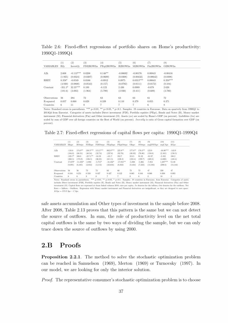
Table 2.6: Fixed-effect regressions of portfolio shares on Home’s productivity:
1990Q1-1999Q4
(1) (2) (3) (4) (5) (6) (7) (8)
VARIABLES B2y Invest2y FDI2ROWlia PEqt2ROWlia B2ROWlia M2ROWlia Fin2ROWlia O2ROWlia
A2h 2.608 -0.113*** 0.0208 0.146** -0.00692 -0.00176 0.00843 -0.00416
(1.925) (0.0324) (0.0207) (0.0609) (0.0308) (0.00432) (0.00642) (0.0398)
RREU 8.358* -0.0549 0.0166 -0.0912 0.0975 0.0313*** 0.00643 0.350***
(4.930) (0.0808) (0.0543) (0.157) (0.0792) (0.0111) (0.0172) (0.104)
Constant -351.5* 32.35*** 0.189 -8.123 2.436 0.0989 -0.678 2.626
(181.6) (3.083) (1.964) (5.799) (2.930) (0.411) (0.609) (3.780)
Observations 56 284 72 63 63 63 61 72
R-squared 0.057 0.068 0.029 0.339 0.110 0.379 0.055 0.371
Countries 6 11 8 7 7 7 6 8
Notes: Standard errors in parentheses. *** p<0.01, ** p<0.05, * p<0.1. Samples: 19 countries in Eurozone. Data on quarterly from 1990Q1 to
2014Q4 from Eurostat. Categories of assets includes Direct investment (FDI), Portfolio equities (PEqt), Bonds and Notes (B), Money market
instrument (M), Financial derivatives (Fin) and Other investment (O). Assets (as) are scaled by Home’s GDP (on percent). Liabilities (lia) are
scaled by sum of GDP over all foreign countries on the Rest of World (on percent). Invest2y is ratio of Gross capital formation over GDP (on
percent).
Table 2.7: Fixed-effect regressions of capital flows per capita: 1990Q1-1999Q4
(1) (2) (3) (4) (5) (6) (7) (8) (9) (10) (11)
VARIABLES BInpc BOutpc FDIInpc FDIOutpc PEqtInpc PEqtOutpc OInpc OOutpc negDNFApc negCApc KGpc
A2h -110.8 174.9** 130.5*** 115.5*** 692.8*** 225.8** 177.8** 178.3** 123.9 -16.80*** -143.9
(104.8) (68.31) (40.54) (32.74) (237.6) (92.76) (88.83) (76.00) (150.0) (2.161) (150.5)
RREU -535.7* 106.0 -217.1** -34.59 -411.7 352.7 313.5 91.32 -81.87 -2.452 108.2
(268.5) (174.9) (106.5) (86.05) (611.5) (238.2) (233.4) (199.7) (409.3) (4.698) (410.4)
Constant 17,679* -11,250* -4,982 -5,715* -44,432* -17,941** -5,826 -5,366 -7,854 1,387*** 9,148
(9,891) (6,445) (3,853) (3,112) (22,616) (8,832) (8,444) (7,223) (14,102) (200.6) (14,142)
Observations 56 56 72 72 63 60 72 72 47 220 47
R-squared 0.104 0.251 0.558 0.427 0.427 0.122 0.065 0.164 0.068 0.300 0.093
Countries 6 6 8 8 7 7 8 8 2 10 2
Notes: Standard errors in parentheses. *** p<0.01, ** p<0.05, * p<0.1. Samples: 19 countries in Eurozone, from Eurostat. Categories of assets
includes Direct investment (FDI), Portfolio equities (E), Bonds and Notes (B), Money market instrument (M), Financial derivatives (Fin) and Other
investment (O). Capital flows are expressed at chain linked volumes 2010, euro per capita. In denotes for the inflows, Out denotes for the outflows. Net
flows = Inflows - Outflows. Regression with Money market instrument and Financial derivatives are insignificant, so they are dropped to save space.
KGpc = DNFApc− CApc.
safe assets accumulation and Other types of investment in the sample before 2008.
After 2008, Table 2.13 proves that this pattern is the same but we can not detect
the source of outflows. In sum, the role of productivity level on the net total
capital outflows is the same by two ways of dividing the sample, but we can only
trace down the source of outflows by using 2000.
2.B Proofs
Proposition 2.2.1. The method to solve the stochastic optimization problem
can be reached in Samuelson (1969), Merton (1969) or Turnovsky (1997). In
our model, we are looking for only the interior solution.
Proof. The representative consumer’s stochastic optimization problem is to choose
37

Table 2.8: Fixed-effect regressions of portfolio shares on Home’s productivity:
2000Q1-2014Q4
(1) (2) (3) (4) (5) (6) (7) (8)
VARIABLES B2y Invest2y FDI2ROWlia PEqt2ROWlia B2ROWlia M2ROWlia Fin2ROWlia O2ROWlia
A2h 1.665 -0.127*** 0.0539* 0.0547*** 0.0598** 0.00332 0.0583** 0.0933***
(1.658) (0.0151) (0.0286) (0.0165) (0.0246) (0.00354) (0.0249) (0.0157)
RREU 14.21** -0.785*** -0.277** 0.0325 -0.256*** -0.0543*** -0.317*** 0.313***
(6.218) (0.0648) (0.108) (0.0645) (0.0966) (0.0139) (0.0932) (0.0593)
Constant 220.2 38.70*** 5.789** 2.672 6.837*** 1.113*** -1.764 5.089***
(166.8) (1.533) (2.885) (1.656) (2.470) (0.355) (2.506) (1.585)
Observations 697 1,016 724 815 818 818 745 753
R-squared 0.009 0.159 0.015 0.014 0.017 0.020 0.025 0.074
Countries 17 18 18 18 18 18 18 18
Notes: Standard errors in parentheses. *** p<0.01, ** p<0.05, * p<0.1. Samples: 19 countries in Eurozone. Data on quarterly from 1990Q1 to
2014Q4 from Eurostat. Categories of assets includes Direct investment (FDI), Portfolio equities (PEqt), Bonds and Notes (B), Money market
instrument (M), Financial derivatives (Fin) and Other investment (O). Assets (as) are scaled by Home’s GDP (on percent). Liabilities (lia) are
scaled by sum of GDP over all foreign countries on the Rest of World (on percent). Invest2y is ratio of Gross capital formation over GDP (on
percent).
Table 2.9: Fixed-effect regressions of capital flows per capita: 2000Q1-2014Q4
(1) (2) (3) (4) (5) (6) (7) (8) (9) (10) (11)
VARIABLES BInpc BOutpc FDIInpc FDIOutpc PEqtInpc PEqtOutpc OInpc OOutpc negDNFApc negCApc KGpc
A2h -490.0 555.9*** -930.6 -670.8 817.3 898.0** 971.3*** 898.4** -10.60 -4.547*** 4.196
(322.1) (184.2) (1,274) (944.3) (535.0) (402.2) (355.8) (399.0) (29.37) (1.467) (29.33)
RREU -2,597** -293.0 -9,734** -6,849* 1,150 791.5 4,309*** 3,306** 26.71 -27.12*** -58.17
(1,208) (690.8) (4,795) (3,553) (2,092) (1,508) (1,342) (1,500) (111.0) (6.271) (110.8)
Constant -19,277 82,147*** 306,584** 261,504*** 118,617** 8,904 12,377 45,427 810.5 505.0*** -134.6
(32,402) (18,533) (128,348) (95,112) (53,703) (40,507) (35,824) (40,217) (2,956) (148.4) (2,953)
Observations 697 697 724 724 815 746 753 750 629 988 629
R-squared 0.010 0.014 0.006 0.006 0.003 0.007 0.022 0.012 0.000 0.025 0.001
Number of countries 17 17 18 18 18 18 18 18 17 18 17
Notes: Standard errors in parentheses. *** p<0.01, ** p<0.05, * p<0.1. Samples: 19 countries in Eurozone, from Eurostat. Categories of assets
includes Direct investment (FDI), Portfolio equities (E), Bonds and Notes (B), Money market instrument (M), Financial derivatives (Fin) and Other
investment (O). Capital flows are expressed at chain linked volumes 2010, euro per capita. In denotes for the inflows, Out denotes for the outflows. Net
flows = Inflows - Outflows. Regression with Money market instrument and Financial derivatives are insignificant, so they are dropped to save space.
KGpc = DNFApc− CApc.
Table 2.10: Fixed-effect regressions of portfolio shares on Home’s productivity:
1990Q1-2007Q4
(1) (2) (3) (4) (5) (6) (7) (8)
VARIABLES B2y Invest2y FDI2ROWlia PEqt2ROWlia B2ROWlia M2ROWlia Fin2ROWlia O2ROWlia
A2h 0.790 0.0439*** 0.0873*** 0.0934*** 0.0547** 0.00912*** 0.0178*** 0.120***
(1.129) (0.0164) (0.0136) (0.0215) (0.0234) (0.00205) (0.00409) (0.0213)
RREU -8.921 0.0402 0.0769 -0.0595 0.0228 0.00649 -0.0156 0.469***
(5.946) (0.0661) (0.0722) (0.121) (0.132) (0.0116) (0.0230) (0.113)
Constant 374.6*** 19.83*** -2.120 -1.647 1.967 -0.218 -1.024** -1.605
(124.4) (1.739) (1.498) (2.383) (2.592) (0.228) (0.455) (2.346)
Observations 344 832 382 426 429 429 372 391
R-squared 0.024 0.013 0.144 0.084 0.020 0.066 0.105 0.080
Countries 17 18 18 18 18 18 18 18
Notes: Standard errors in parentheses. *** p<0.01, ** p<0.05, * p<0.1. Samples: 19 countries in Eurozone. Data on quarterly from 1990Q1 to
2014Q4 from Eurostat. Categories of assets includes Direct investment (FDI), Portfolio equities (PEqt), Bonds and Notes (B), Money market
instrument (M), Financial derivatives (Fin) and Other investment (O). Assets (as) are scaled by Home’s GDP (on percent). Liabilities (lia) are
scaled by sum of GDP over all foreign countries on the Rest of World (on percent). Invest2y is ratio of Gross capital formation over GDP (on
percent).
38

Table 2.11: Fixed-effect regressions of capital flows per capita: 1990Q1-2007Q4
(1) (2) (3) (4) (5) (6) (7) (8) (9) (10) (11)
VARIABLES BInpc BOutpc FDIInpc FDIOutpc PEqtInpc PEqtOutpc OInpc OOutpc negDNFApc negCApc KGpc
A2h -433.5* 939.0*** 1,134*** 1,165*** 2,619** 2,464*** 1,890*** 2,262*** -11.93 -3.491* 11.80
(233.6) (343.0) (366.5) (383.5) (1,016) (846.0) (527.0) (683.7) (34.73) (1.864) (34.93)
RREU -1,540 2,219 4,206** 4,768** 12,311** 11,604*** 8,374*** 10,489*** 70.40 -5.055 -6.303
(1,230) (1,806) (1,948) (2,039) (5,743) (4,439) (2,803) (3,635) (189.3) (8.002) (190.3)
Constant -28,574 14,761 -30,469 -31,424 -144,342 -196,650** -111,099* -141,863* 915.3 287.2 -1,340
(25,732) (37,778) (40,458) (42,339) (112,693) (93,470) (58,178) (75,521) (3,826) (196.8) (3,848)
Observations 344 344 382 382 426 372 391 388 291 760 291
R-squared 0.010 0.025 0.026 0.025 0.017 0.026 0.035 0.031 0.003 0.005 0.001
Countries 17 17 18 18 18 18 18 18 14 18 14
Notes: Standard errors in parentheses. *** p<0.01, ** p<0.05, * p<0.1. Samples: 19 countries in Eurozone, from Eurostat. Categories of assets
includes Direct investment (FDI), Portfolio equities (E), Bonds and Notes (B), Money market instrument (M), Financial derivatives (Fin) and Other
investment (O). Capital flows are expressed at chain linked volumes 2010, euro per capita. In denotes for the inflows, Out denotes for the outflows. Net
flows = Inflows - Outflows. Regression with Money market instrument and Financial derivatives are insignificant, so they are dropped to save space.
KGpc = DNFApc− CApc.
Table 2.12: Fixed-effect regressions of portfolio shares on Home’s productivity:
2008Q1-2014Q4
(1) (2) (3) (4) (5) (6) (7) (8)
VARIABLES B2y Invest2y FDI2ROWlia PEqt2ROWlia B2ROWlia M2ROWlia Fin2ROWlia O2ROWlia
A2h 0.245 -0.0987*** 0.0226 0.0711*** -0.0261 -0.00950** 0.0801 -0.0113
(2.745) (0.0334) (0.0446) (0.0233) (0.0242) (0.00468) (0.0493) (0.0221)
RREU 15.83** -0.507*** -0.264** -0.0985* -0.342*** -0.0324*** -0.240** 0.217***
(6.484) (0.0804) (0.105) (0.0564) (0.0586) (0.0113) (0.117) (0.0525)
Constant 312.1 33.35*** 10.72** 2.199 18.69*** 2.669*** -3.083 17.56***
(281.9) (3.448) (4.574) (2.405) (2.499) (0.482) (5.057) (2.270)
Observations 409 468 414 452 452 452 434 434
R-squared 0.015 0.088 0.017 0.032 0.073 0.024 0.019 0.042
Countries 17 18 18 18 18 18 18 18
Notes: Standard errors in parentheses. *** p<0.01, ** p<0.05, * p<0.1. Samples: 19 countries in Eurozone. Data on quarterly from 1990Q1 to
2014Q4 from Eurostat. Categories of assets includes Direct investment (FDI), Portfolio equities (PEqt), Bonds and Notes (B), Money market
instrument (M), Financial derivatives (Fin) and Other investment (O). Assets (as) are scaled by Home’s GDP (on percent). Liabilities (lia) are
scaled by sum of GDP over all foreign countries on the Rest of World (on percent). Invest2y is ratio of Gross capital formation over GDP (on
percent).
Table 2.13: Fixed-effect regressions of capital flows per capita: 2008Q1-2014Q4
(1) (2) (3) (4) (5) (6) (7) (8) (9) (10) (11)
VARIABLES BInpc BOutpc FDIInpc FDIOutpc PEqtInpc PEqtOutpc OInpc OOutpc negDNFApc negCApc KGpc
A2h -393.7 229.6 -279.3 -255.1 1,174* 787.1* 186.3 339.5 -64.27 -11.94*** 51.20
(546.3) (266.5) (2,078) (1,438) (604.7) (457.8) (645.2) (631.1) (58.76) (2.992) (58.51)
RREU -2,631** -1,129* -11,405** -7,995** -960.6 -885.3 3,208** 2,363 -2.392 -30.16*** -27.36
(1,291) (629.5) (4,919) (3,404) (1,460) (1,086) (1,531) (1,497) (143.5) (7.281) (142.9)
Constant -18,386 119,628*** 296,191 261,868* 109,375* 24,959 96,310 109,446* 6,302 1,293*** -4,905
(56,113) (27,367) (213,297) (147,579) (62,323) (46,994) (66,222) (64,777) (6,040) (308.4) (6,014)
Observations 409 409 414 414 452 434 434 434 385 448 385
R-squared 0.011 0.011 0.014 0.014 0.011 0.010 0.010 0.006 0.003 0.062 0.002
Countries 17 17 18 18 18 18 18 18 17 18 17
Notes: Standard errors in parentheses. *** p<0.01, ** p<0.05, * p<0.1. Samples: 19 countries in Eurozone, from Eurostat. Categories of assets
includes Direct investment (FDI), Portfolio equities (E), Bonds and Notes (B), Money market instrument (M), Financial derivatives (Fin) and Other
investment (O). Capital flows are expressed at chain linked volumes 2010, euro per capita. In denotes for the inflows, Out denotes for the outflows. Net
flows = Inflows - Outflows. Regression with Money market instrument and Financial derivatives are insignificant, so they are dropped to save space.
KGpc = DNFApc− CApc.
39

consumption and portfolio shares to maximize
E
∫ ∞0
1
γcγe−βtdt,−∞ < γ < 1
subject to the stochastic wealth accumudation equation.
dw
w= (ρ− c
w)dt+ dw
1 = nd + nd,∗ + nb
ρ = and + a∗nd,∗ + rnb
dw = ndaσdz + nd,∗a∗σ∗dz∗
σ2w = n2
da2σ2 + n∗d
2a∗2σ∗2
We define the differential generator of the value function V (w, t) by:
Lw[V (w, t)] :=∂V
∂t+(ρ− c
w
)w∂V
∂w+
1
2σ2ww
2∂2V
∂w2(2.B.1)
Given the exponential time discounting, V can be assumed to be of the time-
separable form:
V (w, t) = e−βtX(w)
The formal optimization problem is now to choose c, nd, n∗d, nB to maximize the
Lagrangean expression:
e−βt1
γcγ + Lw[eβtX(w)] + e−βtη[1− nd − n∗d − nB]
Taking partial derivatives of this expression, and canceling e−βt yields:
(c) : cγ−1 = Xw
(nd) : (aXww − η)dt+ cov(dw, aσdz)Xwww2 = 0
(nd,∗) : (α∗Xww − η)dt+ cov(dw, a∗σ∗dz∗)Xwww2 = 0
(nb) : rXww − η = 0
1 = nd + nd,∗ + nb
These equations determine the optimal values for c/w, nd, nd,∗, nb, η as functions
of Xw, Xww. In addition, the value function must satisfy the Bellman equation:
maxc,nd,nd,∗,nb
{1
γcγe−βt + Lw[e−βtX(w)]
}= 0 (2.B.2)
40

We postulate a solution of the form:
X(w) = δwγ
Where δ is the coefficient to be determined. Then, Xw = δγwγ−1;Xww = δγ(γ −1)wγ−2. The F.O.Cs become:
(c) :c
w= (δγ)1/(γ−1)
(nd) : (αδγwγ − η)dt+ cov(dw, ασdz)δγ(γ − 1)wγ = 0
(nd,∗) : (α∗δγwγ − η)dt+ cov(dw, α∗σ∗dz∗)δγ(γ − 1)wγ = 0
(nb) : rδγwγ − η = 0
Substituting for (c
w) into the Bellman equation (2.B.2) and the value function
(2.B.1) leads to:
1
γ[(δγ)1/(γ−1)w]γ − βδwγ + [ρ− (δγ)1/(γ−1)]wδγwγ−1 +
1
2σ2ww
2δγ(γ − 1)w(γ−2) = 0
⇒ˆ( cw
)= (δγ)1/(γ−1) =
β − ργ − 1
2γ(γ − 1)σ2
w
1− γ
The F.O.Cs dividing by (δγwγ):
(nb) : r =η
δγwγ
(nd) :
(a− η
δγwγ
)dt = (1− γ)cov(dw, aσdz)
(nd,∗) :
(a∗ − η
δγwγ
)dt = (1− γ)cov(dw, a∗σ∗dz∗)
By substitute the equilibrium value ofˆ( cw
)into the Bellman equation, we find:
δ =1
γ
ˆ( cw
)γ−1
From this system of F.O.Cs, and with the country-specific shocks (cov(dz, dz∗) =
41

0), we get the macroeconomic equilibrium in Home country:
nd =1
(1− γ)
(a− r)a2σ2
nd,∗ =1
(1− γ)
(a∗ − r)a∗2σ∗2
nb = 1− nd − nd,∗c
w=
1
1− γ
(β − ργ +
1
2γ(1− γ)σ2
w
)ψ =
1
(1− γ)
(ρ− β − 1
2γ(1− γ)σ2
w
)ρ = and + a∗nd,∗ + rnb
σ2w = nd
2a2σ2 + nd,∗
2a∗2σ∗2
Similar steps for the Foreign country.
Finally, the safe assets market clearing condition (b + b∗ = nbw + nb,∗w∗ = b)
implies the safe interest rate as:
r =[1/(aσ2) + 1/(a∗σ∗2)] + (1− γ)[b/(w + w∗)− 1)]
1/(a2σ2) + 1/(a∗2σ∗2)(2.B.3)
�
Proposition 2.4.1
Proof.
CA = (andw + a∗nd ∗ w + rnBw −c
ww − ndwψ − nfw∗ψ∗)dt
+ [(1− nd)ndw + (1− nf )nfw∗]aσdz − [ndn∗dw + nfn
∗fw∗]a∗σ∗dz∗
KG = k∗daσ∗dz∗ − kfασdz = n∗dwa
∗σ∗dz∗ − nfw∗aσdz
With the assumption that Cov(dz, dz∗) = 0,
Cov(CA,KG) = [−n∗dw(ndn∗dw + nfn
∗fw
∗)a∗2σ∗2 − nfw∗((1− nd)ndw + (1− nf )nfw∗)a2σ2]dt < 0
V ar(CA) = [((1− nd)ndw + (1− nf )nfw∗)2a2σ2 + (ndn
∗dw + nfn
∗fw
∗)2a∗2σ∗2]dt
V ar(KG) = [n∗d2w2a∗2σ∗2 + n2fw
∗2α2σ2]dt
corr(CA,KG) =cov(CA,KG)√
V ar(CA)√V ar(KG)
< 0
�
42

2.C Extended model: Safe assets scarcity
We assume that the exogenous supply of safe assets is different across countries.
In each country, the share of safe assets over the domestic wealth is different. This
share can be intepreted as the capitalization rate of financial assets over domestic
income as in Farhi, Caballero and Gourinchas (2008). Indeed, an advanced econ-
omy have a higher capitalization rate than the developing economies. Since the
capitalization determines the autarky safe interest rate, it shapes the pattern of
capital flows. In comparision with an exogenous total supply of safe assets in the
main text, this extended model can capture the pattern of capital flows between
the advanced economy (Home) and the developing economy (Foreign).
The structure of model is almost the same as in the main text. The only difference
is that the exogenous supply of safe assets is δw at Home while δ∗w∗ at Foreign.
The key feature is that Home has a higher supply of safe assets:
δ > δ∗ (2.C.1)
Autarky equilibrium
At autarky, each agent only allocate her wealth between the domestic risky asset
and the safe assets. We focus on the Home economy, but the analysis for Foreign
is similar. The equilibrium portfolio shares are:
nd =1
1− γa− ra2σ2
nb = 1− nd
The market clearing condition on the safe assets is as following:
nbw = δw ⇔ 1− 1
1− γa− rH
a2σ2= δ
Therefore, the Home autarky safe interest rate is:
rH = a− (1− γ)(1− δ)a2σ2 (2.C.2)
It is clear that the autarky safe interest rate is increasing on the capitalization
rate over output (δ): given the demand, a higher supply of safe assets reduces the
safe asset’s price and therefore, depresses the interest rate.
Similarly, the autarky safe interest rate in the Foreign economy is:
rF = a∗ − (1− γ)(1− δ∗)a∗2σ∗2 (2.C.3)
43

Integration equilibrium
At integration, each agent can invest on the foreign risky asset. The equilibrium
portfolio shares are the similar to the model in the main text, but only the equilib-
rium safe interest rate is modified. In details, one world interest rate (rw) prevails
to clear the world market for safe assets.
nd = nf =1
1− γα− rw
a2σ2
nd,∗ = nf,∗ =1
1− γα∗ − rw
a∗2σ∗2
nb = nb,∗ = 1− nd − nd,∗
The world market clearing condition equalizes the aggregate demand to the ag-
gregate supply of safe assets.
nbw + nb,∗w∗ = δw + δ∗w∗
Therefore, the world safe interest rate is as following:
rw =[1/(aσ2) + 1/(a∗σ∗2)]− (1− γ)(1− δ)
1/(a2σ2) + 1/(a∗2σ∗2)(2.C.4)
whereby, the world supply of safe assets is an average value of safe assets supplies
across two countries:
δ ≡ w
w + w∗δ +
w∗
w + w∗δ∗ ⇒ δ > δ > δ∗ (2.C.5)
We can show that the world interest rate is the linear combination of the autarky
safe interest rate. Therefore, the world interest rate is between the highest and
lowest autarky interest rate. For j = H,F ,
rw = ν + ΣjλjΣjµ
jrj ⇒ rH > rw > rF (2.C.6)
whereby,
ν ≡ (w∗
w + w∗aa∗2σ∗2 +
w
w + w∗a∗a2σ2)/(a2σ2 + a∗2σ∗2)
λH ≡ a∗2σ∗2
a2σ2 + a∗2σ∗2
λF ≡ a2σ2
a2σ2 + a∗2σ∗2
µH ≡ w
w + w∗
µF ≡ w∗
w + w∗
44
Exporter of Safe assets
At the world integration, the difference between the supply and demand of safe
assets in each country is evaluated at the world safe interest rate:
δw − nbw = δ − δ > 0 (2.C.7)
δ∗w∗ − nb,∗w∗ = δ∗ − δ < 0 (2.C.8)
Since Home has a higher capitalization of safe assets (δ > δ > δ∗), its supply
of asset is greater than its domestic demand at the integration. Home economy
exports the safe assets to the Foreign. Therefore, the Home agent enjoys the
positive return on the safe assets which is paid by the Foreign one5 .
rw(δ − nb)w > 0 (2.C.9)
On this model, the Home enjoys a positive capital gains by a comparative advan-
tage on providing the safe assets, a mechnism is emphasized by Farhi, Caballero
and Gourinchas (2008).
2.D Extended model: Exorbitant privilege
We allow the supply of safe assets is endogenously determined at equilibrium.
The idea is employed from Farhi and Maggiori (2016) where one economy with
risk-neutral utility issues the bonds to the rest of world whose a risk-averse utility.
We extend the model in the main text by allowing the Home agent is a less risk
averse than Foreign. We will show that this difference on the risk-taking behavior
results in the positive supply of safe assets at equilbirum.
The structure is the same as the model in the main text. Now, the Home agent
has a less risk averse coefficent than the Foreign one.
(1− γ) < (1− γ∗) (2.D.1)
Equilibrium
The equilibrium portfolio shares for Home are as following: The world market
clearing condition for the safe assets captures the zero net supply at equilibrium,i.e,
total supply is exactly equal to total demand for safe assets.
nbw + nb,∗w∗ = 0 (2.D.2)
5By world market clearing condition (2.C.5), rw(δ − nb)w = rw(nb,∗ − δ∗)
45

Home Foreign
nd =1
1− γa− ra2σ2
; nf =1
1− γ∗a− ra2σ2
nd,∗ =1
1− γa∗ − ra∗2σ∗2
; nf,∗ =1
1− γ∗a∗ − ra∗2σ∗2
nb = 1− nd − nd,∗; nb,∗ = 1− nf − nf,∗
Plugging the portfolio share (nb, nb,∗) into the market clearing condition, we end
up with the safe interest rate:
r =
(w
1− γ+
w∗
1− γ∗)(
1
aσ2 + a∗σ∗2)− (w + w∗)
(w
1− γ+
w∗
1− γ∗)(
1
a2σ2+
1
a∗2σ∗2)
(2.D.3)
For the positive safe interest rate, the Home agent needs to be risk neutral enough.
r > 0⇔ (1− γ) < ξ(γ∗) ≡ w
(w + w∗)(aσ2a∗2σ∗2
aσ2 + a∗σ∗2)− w∗
1− γ∗
(2.D.4)
Whereby, the threshold is decreasing on (1− γ∗): ∂ξ(γ∗)
∂(1− γ∗)< 0.
The threshold is intuitive since more risk averse the Foreign agent is (higher (1−γ∗)), more risk neutral the Home agent should be: (1−γ) needs to be lower. This
condition would ensure that Home economy would supply the safe assets to Foreign
economy. This result is similar to the model by Caballero and Farhi (2014), in
which one Neutral agent with the risk-neutral utility issues the safe assets to the
Knightian agent with infinite risk averse coefficient, so that the condition (2.D.4)
is always satisfied.
Exporter of safe assets
At the integration equilibrium, the Home agent less risk averse (γ > γ∗) would
issues the safe asset to the Foreign agent. This intuition follows by the result that:
γ > γ∗ ⇔ (B = nbw < 0;B∗ = −B = nb,∗w∗ > 0) (2.D.5)
It means that the Home agent invests the risky assets more than her wealth while
the Foreign investment on the risky assets is less than her wealth.
Kd +Kd,∗ = W −B > W (2.4.6)
Kf +Kf,∗ = W ∗ −B∗ < W ∗ (2.4.7)
46

The Home economy borrows a fraction of B∗ from the Foreigng one to invest on
the risky assets. With the constant portfolio shares, the differential rate of returns
that Home agent gains is:
B∗(and + a∗nd,∗ − r) (2.4.8)
Plugging the equilibrium portfolio share and the safe interest rate (2.D.3), aftersome manupulation, we end up with:
B∗
1
(1− γ)
(a− a∗)2
(a2σ2 + a∗2σ∗2)+
1
aσ2+
1
a∗σ∗2
1
a2σ2+
1
a∗2σ∗2
w∗(γ − γ∗)
(1− γ∗)w + (1− γ)w∗+
(w + w∗)(1
a2σ2+
1
a∗2σ∗2)−1
(w
1− γ+
w∗
1− γ∗)
> 0 (2.4.9)
This term is coined as the exorbitant priviledge (Gourinchas, Rey and Govillot
(2010)) which is the rent that one country with the reserve currency (like United
States) can gain by borrowing with low cost from the Rest of Word in order to
invest on the risky assets with higher rate of returns. The exorbitant rent is
increasing on the value of safe assets (B∗). The rent is also increasing on the
Foreign’s coefficient of relative risk averse since, when the Foreign agent become
more risk averse, she demands more safe assets. And the Home agents can enjoy
a higher rent on issuing the safe assets. Finally, the rent is also increasing on the
risky rate of returns while decreasing on the safe interest rate. Therefore, a higher
differential rates of return between the risky and safe assets raises the exorbitant
privilege.
The exorbitant rent for the Home agent arises in our model because of two reasons.
The first reason is the heterogeneity in the risk aversion across countries. The
Home agent is less risk averse than the Fereign one. Therefore, she is provider
of safe assets at equilibrium.This intuition is captured by the positive term (γ −γ∗). The Foreign agent is more risk averse, then she demands the safe assets at
equilibrium. More risk averse the Foreign agent is, more demand for safe assets
and higher safe premium that she has to pay for the Home agent. This intuition
is captured by the term (1− γ∗). The second reason is the enriched portfolio with
two risky assets and one safe assets. As long as there is difference on the rate of
returns between the Home and Foreign risky assets, the risk diversification would
help the Home agent to allocate her wealth by the most efficient way. This reason
is captured by the positive term (a− a∗)2. In sum, the Home agent earns the rent
on her investment as the award to her higher risk-taking attitude in comparision
with the Foreign counterpart.
47

Chapter 3
Non-Linear Pattern of
International Capital Flows
Abstract
The empirical analysis on one panel sample of 165 countries from 1980 to 2013
reveals one non-linear pattern of dependence of the net total capital inflows on the
productivity growth. We rationalize this new finding by building up one multi-
country OLG economy to show that there exists one threshold over which an
increase of the productivity growth raises the net total capital inflows as implied
by the Neo-Classical growth model. Below that threshold, however, the reversal
pattern holds (allocation puzzle). The financial frictions and the world average
productivity growth rate are the key elements of the threshold.
48

3.1 Introduction
The past decades witnesses a diversification of the pattern of the international
capital flows across the developing and advanced economies (Figure 3.1.1). On
one hand, the exporters of capital can be the advanced economies with the low
growth rates (Japan (JPN), Germany (DEU), Netherlands (NLD)) or emerging
economies with the high growth rates (China (CHN), Korea (KOR), Singapore
(SGP)). On other hand, the importers of capital can be the slow-growing advanced
economies (United States (USA), United Kingdoms (GBR), Australia (AUS)) or
the fast-growing emerging economies (Cyprus (CYP), Thailands (THA), Pakistan
(PAK)). The mixed patterns of the net total capital inflows raise the concern over
the linear dependence of the net total capital inflows on the productivity growth
rate.
Figure 3.1.1: Pattern of International capital flows by countries
Notes: All variables are averaged over 1980-2013. The net total capital inflows is the
negative value of the current account as percentage of GDP and GDPpc is real output-
side GDP per capita at constant 2005 national price.
The Neo-Classical growth model predicts that one country growing faster would in-
vest more and experience a net total capital inflow. The recent empirical evidence1
documents that the fast-growing economies tend to experience a net total capital
outflow (Allocation puzzle). Our paper rationalizes both of these two arguments
1Prasad, Rajan, and Subramanian (2007),Gourinchas and Jeanne (2013)
49

by showing that the pattern of the net total capital inflows on the productivity
growth rate is non-linear: the allocation puzzle exits but there is one threshold
over which the prediction by the Neo-Classical growth model works.
We prove the non-linear pattern of international capital flows by both the empir-
ical evidences and the theoretical model. On empirical ground, the analysis of a
sample of 165 countries from 1980 to 2013 shows that the allocation puzzle only
applies for the middle range of the productivity growth rate. For the low and high
range of the productivity growth rate, however, an increase of the growth rate
raises the net total capital inflows. In sum, the empirical evidence demonstrates
that there exists one threshold over which the net total capital inflow is increasing
on the productivity growth rate.
On theoretical ground, we construct one multi-country economy where each coun-
try differs by the level of productivity growth and the financial frictions. At
autarky, the interest rate depends on the domestic productivity growth rate and
financial frictions. At integration, the interest rate is equalized across countries
and depends on the world average growth rate and the financial frictions. With the
free mobile capital, the capital flows into the country which has a higher interest
rate at autarky than at integration. This condition turns out to be one threshold
only over which there exits the positive relationship between the net total capital
inflows and the productivity growth rate, as implied by the Neo-Classical growth
model. In sum, the interaction between the productivity growth rate and the fi-
nancial frictions can generate one non-linear dependence of the net total capital
inflows on the productivity growth rate.
Our paper belongs to the literature on the relationship between the international
capital flows and the productivity growth rate (see Gourinchas and Rey (2015)
for a recent survey). Lucas (1990) questions why the capital does not flow to the
poor countries in which, because of the capital scarcity, the marginal product of
capital is higher than in the advanced economies. Gourinchas and Jeanne (2013)
raises a deeper question why the capital does not flow to the emerging economies
which grow faster and invest more than the advanced economies. Their models,
however, are the small open economies. Therefore, there is no implication for the
pattern of capital flows across the developing and advanced economies. Moreover,
the direction of capital flows is linear in the sense that the net total capital flows
can either flow into or out of a small open economy. Our paper proposes an ex-
tension of these models to the multi-country economy which takes into account
the interaction of the productivity growth rate and the financial friction levels.
Therefore, we can build up one threshold on the productivity growth rate to ac-
50

count for the non-linear pattern of the international capital flows.
There are also many multi-country models to account for the dependence of inter-
national capital flows on the productivity growth. In Gertler and Rogoff (1990),
the capital market imperfections are endogenously determined by the asymmet-
ric information problem which is less severe in the rich countries. Therefore, the
domestic loan rate is lower in the rich than in the poor economies, which implies
that the investment demand is higher in the rich than in the poor. In Boyd and
Smith (1997), the rich economy also has a higher investment demand because
its high income can afford for the agency cost induced by the asymmetric infor-
mation on lending. In Matsuyama (2004), the rich country having the higher
initial capital stock would converge to a higher steady sate capital accumulation
and also has a higher investment demand than the poor economies. This role of
the initial capital stock is quite similar as in Dechert and Nishimura (2012): with
an unconvex technology, an optimal path converges to a steady state only if the
inital capital stock is above a critical value. The main mechanism of these models
is that the capital flows from the poor to rich economies to finance a higher invest-
ment demand in the rich economies. Our paper takes into account the differential
investment demands but focuses more on the differential saving supplies as the
driver of the international capital flows.
Farhi, Caballero and Gourinchas (2008) focus on the savings of the developing
economies which have a higher output growth rate than the advanced economies.
The supply of financial assets, however, is lower in the developing than in the
advanced economies. The low supply of financial assets, in turn, results in a lower
interest rate in the developing economies. Therefore, the savings flows from the
developing to the advanced economies on seeking the financial assets. While their
paper focuses on the supply side, ours focuses on the demand side for the financial
asset. Indeed, on country with a low saving wedge (i.e, a low capital taxation),
the savings is high and then, the demand for the assets is high. The high demand
raises the asset’s price and depresses the autarky interest rate. At integration, the
capital flows out of that country for a higher foreign interest rate. Therefore, in
our model, the heterogeneity on the saving wedge shapes the pattern of interna-
tional capital flows.
Coeurdacier, Guibaud and Jin (2015) analyze the differential age-saving profiles
between the developing (China) and advanced economy (United States) by focus-
ing the borrowing constraint which is tighter on the former. The aging population
in China raises the savings by the middled-age people more than the borrowing
by the young people. The case, however, is reversal in the United States. There-
51

fore, there is excess saving in China and capital flows to US for the interest rate
is equalized across countries. The excess saving in the developing economies at
autarky is also the key mechanism in Angeletos and Panousi (2011), in which
the high level of the idiosyncratic risk motivates the precautionary saving in the
developing economies. Our model also generates the high saving rate in the de-
veloping economies, but the autarky capital accumulation is not necessary high
in the developing economies like the aforementioned papers. In particular, one
economy with a low saving wedge and high investment wedge can have both the
high savings and low capital accumulation.
The paper is structured as follows. After the introduction, section (3.2) provides
the empirical evidence on the non-linear pattern of international capital flows.
Then, section (3.3) lays out the model and characterize the equilibrium. Section
(3.4) presents the core result on the pattern of international capital flows across
countries. And section (3.5) concludes and is followed by the Appendix.
3.2 Empirical analysis
Table 3.1: Fixed-effect regression of the long-run net total capital inflows: 65
Non-OECD countries (1980-2013)
(1) (2) (3)
VARIABLES anegCA2y anegCA2y anegCA2y
Output per capita growth rate (aGDPpcgrowth) -0.825*** - -
(0.295)
Saving wedge (atau) - 8.155** -
(3.824)
Investment wedge (agammaPL) - - -0.709***
(0.256)
Openness (akaopen) -1.399*** -1.836*** -1.118*
(0.518) (0.546) (0.621)
Constant 3.902*** -1.213 1.723***
(0.789) (1.804) (0.593)
Observations 65 63 48
R-squared 0.232 0.188 0.229
Notes: standard errors in parentheses. *** p<0.01, ** p<0.05, * p<0.1. (anegCA2y)
is the average of current account-output ratios (%) over 1980-2013; (aGDPpcgrowth) is
the average of the output-per-capita growth rates; (atau) is the average of saving wedges;
(agammaPL) is the average of investment wedges; (akaopen) is the Chinn-Ito index of
capital account openness. Data on the net total capital inflows (anegCA2y) is from
Alfaro, Kalemli-Ozcan and Volosovych (2014); the output-per-capita growth rate is the
per capita value of the real output at constant 2005 national prices from Penn World Table
8.1. The saving wedge = (lending rate - deposit rate)/lending rate. The investment wedge
= (PMPKL-lending rate)/PMPKL, where PMPKL is the estimated marginal product of
capital taking into account the difference in price of output and capital, and the share
of the reproducible capital (Caselli and Feyrer (2007)). Variables are the average value
over 1980-2013, on percentage. See data appendix for more details.
52

Table 3.1 reports the estimation result of the net total capital inflows on the pro-
ductivity growth rate and on the interest rate wedges for 65 Non-OECD countries,
as the sample analyzed by Gourinchas and Jeanne (2013). Column 1 shows that
one country with a higher productivity growth rate tends to export the capital, a
phenomenon labeled as the allocation puzzle: one country which grows faster and
invests more tends to export the capital to the rest of world. Column 2 confirms
their result that the net total capital inflow is increasing on the saving wedge
while column 3 shows that it is decreasing on the investment wedge. In short, the
regression on the sample of Non-OECD countries confirms one linear dependence
of the net total capital inflows on the productivity growth rate.
Table 3.2 presents the regression result of the net total capital inflows on the pro-
ductivity growth rate for a sample including both OECD and Non-OECD coun-
tries. Column 1 and 2 show that the coefficient of the productivity growth rate is
insignificant, up to its quadratic term. Column 3 demonstrates that the impact
of the productivity growth rate on the net total capital inflows is significant only
when we consider the impact as one cubic function. In sum, the regression on the
full sample proves one non-linear dependence of the net total capital inflows on
the productivity growth rate.
Table 3.3 examines the role of the saving wedge on the accounting for the pattern
of the net total capital inflows. Column 1 shows that the relationship between the
net total capital inflows and the saving wedge follows one cubic function. Column
2 and 3 trace down the pattern of the savings, as the driver of the net total capital
inflows (by definition, Net total capital inflows = Investments - Savings). The
savings is one cubic fuction of the wedge, and the sign is reversal to the sign of the
net total capital inflows. The table provides the strong evidences that the saving
wedge can account for the pattern of the net total capital inflows.
Figure 3.2.1 plots the regression results of the net total capital inflows on the
productivity growth rate and the interest rate wedges. On the panel A, the allo-
cation puzzle only applies for the middle range of value of the productivity growth
rate. At low or high value, however, an increase of the productivity growth rate
raises the net total capital inflows. On the panel B, the net total capital inflows
is increasing on the saving wedge only for the middle range of wedge. For low
and high saving wedges, it is decreasing on the wedge. Since one country with a
high productivity growth rate tends to have a low saving wedge (indeed, for the
full sample, corr(aGDPpcgrowth, atau) = −0.3724), the saving wedge is a strong
candidate to explain the relationship between the net total capital inflows and the
productivity growth rate. On the panel C, the net total capital inflows has one
53

Table 3.2: Fixed-effect regression of the long-run net total capital inflows: 169
countries (1980-2013)
(1) (2) (3)
VARIABLES anegCA2y anegCA2y anegCA2y
Output-per-capita growth rate (aGDPpcgrowth) 0.424 0.0852 1.936**
(0.373) (0.669) (0.783)
(aGDPpcgrowth)2 - 0.0585 -1.127***
(0.0958) (0.304)
(aGDPpcgrowth)3 - - 0.111***
(0.0272)
Constant 2.962*** 3.173*** 4.327***
(0.991) (1.052) (1.043)
Observations 162 162 162
R-squared 0.008 0.010 0.105
Notes: standard errors in parentheses. *** p<0.01, ** p<0.05, * p<0.1. (anegCA2y)
is average of the current account-output ratios over 1980-2013. (aGDPpcgrowth) is the
average of output-per-capita growth rates over 1980-2013. Data on the net total capital
inflows is from Alfaro, Kalemli-Ozcan and Volosovych (2014); the output-per-capita
growth rate is the per capita value of the real output at constant 2005 national prices
from Penn World Table 8.1. Variables are the average value over 1980-2013, on percentage.
See data appendix for more details.
Table 3.3: Fixed-effect regression of the long-run net total capital inflows and
savings: 169 countries (1980-2013)
(1) (2) (3)
VARIABLES anegCA2y aS2GNI aS2y
Saving wedge (atau) -252.0*** 89.40** 246.6***
(53.71) (43.30) (58.92)
(atau)2 868.6*** -317.3*** -865.6***
(125.3) (101.1) (137.6)
(atau)3 -780.8*** 271.2*** 777.0***
(91.03) (73.46) (99.97)
Constant 15.38** 19.18*** 10.97
(7.776) (6.256) (8.515)
Observations 169 166 166
R-squared 0.423 0.104 0.373
Notes: standard errors in parentheses. *** p<0.01, ** p<0.05, * p<0.1.
(anegCA2y) is the average of current account-output ratios over 1980-2013;
(aS2GNI, aS2y) are the average of savings over output ratios over 1980-2013; (atau)
is the average of saving wedges over 1980-2013. Data on the net total capital inflows
is from Alfaro, Kalemli-Ozcan and Volosovych (2014). Two measures of total sav-
ings: Gross savings as percentage of Gross National Income (GNI) (S2GNI) and
Gross savings as percentage of GDP (S2y). The saving wedge = (lending rate -
deposit rate)/lending rate. All these latter data are from World Development Indi-
cators. Variables are the average value over 1980-2013. See data appendix for more
details.
54

linear relationship with the investment wedge. This proves that only the invest-
ment wedge can not fully account for the pattern of the net total capital inflows.
We need to take into account both the saving and investment wedges to explain
the pattern of the net total capital inflows and the productivity growth rate. The
empirical analysis shows that the net total capital inflows has one non-linear rela-
tionship with the productivity growth rate. Indeed, there exists one threshold of
the productivity growth rate, over which an increase of productivity growth raises
the net total capital inflows.
In the next section, we develop a theory of international capital flows taking into
account the interaction between the productivity growth rate and the interest rate
wedges to be consistent with these empirical evidences.
3.3 Theory
The world economy includes many large open countries, populated with the over-
lapping generations of households who live for two periods2. Each household
supplies one unit of labor when young and retires when old. All countries use the
same technology to produce one homogeneous good, which is used for consumption
and investment, and is traded freely and costlessly. Preferences and production
technologies have the same structure and parameter values across countries. The
capital is free mobile but labor is immobile across countries. Finally, firms are
subject to changes in the country-specific productivity levels and labor forces.
Specification of the thereotical model
The model is constructed to be consitent with the empirical evidences. The em-
pirical analysis uses the cross-section data sample for about 160 economies, both
OECD (advanced economy) and Non-OECD (developing economy). By taking
the average over the time period, we want to focus on the long-run measure of
variables. By collecting data on 160 economies, we want to capture the pattern of
capital flows for both the advanced and developing economies. These two empiri-
cal features will be captured by the theoretical model.
On the theoretical model, we employ an OLG framework where each agent lives
for two periods: young and old. Since we focus on the steady state of the economy,
all the theoretical implications apply for the long run variables, which are proxied
2The model is an extension of small open economy on Gourinchas and Jeanne (2013) to
multi-country economy, but with OLG framework like Coeurdacier, Guibaud and Jin (2015).
55

Allocation puzzle
-2 2 4 6 8 10aGDPpcgrowth
-10
-5
5
10
anegCA2y
Panel A: Net total capital inflows and Productivity growth rate
0.2 0.4 0.6 0.8atau
-40
-20
20
40
anegCA2y
Panel B: Net total capital inflows and saving wedge
Panel C: Net total capital inflows and investment wedge
Figure 3.2.1: The regression result of the Net total capital inflows (anegCA2y) on
the productivity growth rate (aGDPpcgrowth), the saving wedge (atau) and the
investment wedge (agammaPL)
Notes: anegCA2y = 4.327 + 1.936 ∗ aGDPpcgrowth − 1.127 ∗ (aGDPpcgrowth)2 + 0.111 ∗(aGDPpcgrowth)3; anegCA2y = 15.38 − 252 ∗ atau + 868.6 ∗ (atau)2 − 780.8 ∗ (atau)3; anegCA2y = 3.72 −−3.29 ∗ agammaPN.
56

by the average over the time period 1980-2013 in the data sample. On other word,
even we use the Ramsey multi-period living agents, we would also focus on the
steady state and use the cross-section data sample.
Furthermore, we employ a multi-country model each one of which has an influ-
ence on the world equilibrium. This structure allows us to derive the implication
for the large-open developed economies and developing economies. This structure
is implemented by Coeurdacier, Guibaud and Jin (2015) to analyze the global
imbalances between United States and China. Although not all 160 economies in
our sample can be large enough to affect the other economies, one large economy
can be thought as a combination of small open economies. For example, VietNam
and Singapore are the small economies, but the Association of Southeast Asian
Nations (ASEAN) can be considered to be a large economy.
In sum, the multi-country OLG model is appropriate to account for the cross-
section data analysis over a large sample of countries in the previous empirical
section.
3.3.1 Production
For any country j, let Kt denote the capital stock at the begining of period t, and
Nt the total labor input employed in period t. The output is:
Yt = (Kt)α(AtNt)
(1−α)
where 0 < α < 1, and At is country-specific productivity. The capital stock is
fully depreciated and is augmented by investment It−1, with the law of motion:
Kt = It−1
The factor markets are perfect competitive so that each factor, capital and labor,
earns its marginal product. Given the rental rate of capital (Rt), the capital stock
and the wage rate per unit of labor are as following:
Kt = (α
Rt
)1/(1−α)AtNt
wt = (1− α)KtαAt
(1−α)Nt−α = (1− α)(
α
Rt
)α/(1−α)At
Given the expected rental rate of capital at the next period (Ret+1), the investment
demand by firm at time t is:
It = Kt+1 = (α
Ret+1
)1/(1−α)At+1Nt+1
Let gAt and gNt denote the growth rate of productivity and of the size of consecutive
cohorts, respectively, so that: At = (1 + gAt )At−1 and Nt = (1 + gNt )Nt−1.
57

3.3.2 Consumption
For any country j, one household born in period t earns the competitive wage
rate wt. Let cyt and cot+1 denote the consumption of an agent when young and old
respectively. The lifetime utility of a household born in period t is:
Ut = u(cyt ) + βu(cot+1)
with standard isoelastic preferences u(c) = (c1−1/σ − 1)/(1− 1/σ) where σ is the
intertemporal elasticity of substitution coefficient. The discount factor β satisfies
0 < β < 1.
Let st denote the saving at the end of period t of an agent born at t. The sequence
of budget constraints is as following:
cyt + st = wt (3.3.1)
cot+1 = Rdt+1st + zt+1 (3.3.2)
When young, each individual works to receive the wage rate. She allocates the
income between consumption and saving as deposit into the bank. When old, she
receives the deposit interest rate (Rdt+1) on her savings and the income transfer
(zt+1) from the government.
Let denote Rlt+1 is the lending interest rate which prevails to clear capital mar-
ket, which equalizes the total saving supplied by households and total investment
demanded by firm. We assume that the government levies the tax rate (τ) on
the domestic saving. Therefore, each individual only receives the after-tax rate of
return paid by the bank.
Rdt+1 = (1− τ)Rl
t+1 (3.3.3)
In general, τ can illustrate the financial frictions (taxation, corruption...) which
generate a gap between the lending interest rate (Rlt+1) and the deposit interest
rate Rdt+1 which accrues to the saving by households.
Plug (3.3.3) into (3.3.2), the consumption at old age of one agent born at t is:
cot+1 = (1− τ)Rlt+1st + zt+1
By solving the utility maximization problem, the wedge enters the Euler equation,
then, affects the saving rate by the young agent.
u′(cyt )
u′(cot+1)= β(1− τ)Rl
t+1 ⇒ st =wt − (β(1− τ)Rl
t+1)−σzt+1
1 + β−σ((1− τ)Rlt+1)(1−σ)
Therefore, on aggregation, the total supply of savings at time t follows:
St = Ntst =wtNt − (β(1− τ)Rl
t+1)−σNtzt+1
1 + β−σ((1− τ)Rlt+1)(1−σ)
(3.3.4)
58

3.3.3 Bank
For any country j, one representative bank collects saving to lend to firms. It
covers the capital taxation (γ) which is a fraction of total revenue gained by
lending to the firms.
Πt = RtLBt−1 −Rl
tDBt−1 − γRtL
Bt−1
The deposit market clearing condition requires the total demand of the deposit
DBt−1 to be equal to the total supply of the saving by households St−1. The loans
market clearing condition requires the total demand of the investment It−1 to be
equal to the total supply of the fund by bank LBt−1.
Autarky economy
At autarky, the total supply of the fund is equal to the total demand of the deposit.
In other words, the total saving supply is equal to the total investment demand.
This condition gives the equilibrium lending interest rate (Rlt).
DBt−1 = LBt−1 ⇔ St−1 = It−1
The zero-profit condition and the autarky interbank market clearing condition
imply that the capital taxation (γ) generates an investment wedge between the
lending interest rate and the rental rate of capital.
Rt =Rlt
(1− γ)
Integration economy
At financial integration, one international bank receives all deposits from house-
holds and lends to firms across countries. Then, one world interest rate (Rl,wt )
prevails such that the world total demand of investments equals to the world total
supply of savings.
ΣjSjt−1 = ΣjI
jt−1
The zero profit condition for banks still implies that the domestic rental rate of
capital is related to the world lending interest rate by the investment wedge3
Rjt =
Rl,wt
(1− γj)3One bank collects an amount of deposit M j
t−1 from the world market with the interest rate
Rl,wt and lends all of this deposit to domestic firm to receive the rental rate of capital Rjt . With
the transaction cost γj , the zero-profit condition implies that Rjt (1− γj) = Rl,wt .
59

Therefore, one country with a high investment wedge would suffer a high cost of
capital, even the lending interest rate is equalized to the world rate.
3.3.4 Government
The government collects the taxation and transfers all tax revenue to the house-
holds4. We assume that only the old agents receive transfer. This assumption
helps us to focus on the distortion that the taxation generates on the consump-
tion and saving. In the Appendix, we relax this assumption by introducing the
public expenditure. In details, the income transfer per each old agent in the
country j at autarky follows:
zt =ZtNt−1
≡ τRltNt−1st−1 + γRtIt−1
Nt−1
(3.3.5)
whereby, the first term is the tax revenue by taxing the saving and the second
term is the tax revenue by taxing the investment.
At integration with one world common lending interest rate, the income transfer
is:
zjt =Zjt
N jt−1
≡τ jRl,w
t N jt−1s
jt−1 + γjRj
tIjt−1
N jt−1
3.3.5 Equilibrium
Autarky equilibrium
Definition 3.3.1. The autarky temporary equilibrium.
Given the value determined by the last period (St−1) and the expected interest rate
(Rl,et+1), the temporary equilibrium is a list of prices (Rl
t, Rdt , Rt, wt) and allocations
(cyt , cot , st, It), aggregate variables (Kt, St, Lt, Yt) such that5 :
1. Profit maximization and Utility maximization subjected to budget constraint.
2. Market clearing condition:
4This approach is also applied by Gourinchas and Jeanne (2013).5Indeed, we have:
• Price: Rt =Rlt
(1− γ);Rdt = (1− τ)Rlt and wt = (1− α)At
[α(1− γ)
Rlt
]α/(1−α)
≡ w(Rlt)
• Allocation: LDt = Nt;Kt =
[α(1− γ)
Rlt
]1/(1−α)
AtNt ≡ K(Rlt);Yt =
[α(1− γ)
Rlt
]α/(1−α)
AtNt;
st =w(Rlt)− (β(1− τ)R
l,et+1)−σzt+1
1 + β−σ(Rl,et+1(1− τ))(1−σ)
≡ s(Rlt, Rl,et+1); c
yt = w(Rlt)− s(R
lt, R
l,et+1); cot = Rltst−1
60

a Labor market: Lt = Nt
b Capital market: Kt = St−1 = Nt−1st−1
c Good market: Ntcyt +Ntst +Nt−1c
ot = Yt
Definition 3.3.2. The autarky inter-temporal equilibrium.
Given an initial lending interest rate (Rlt=0), an inter-temporal equilibrium with
perfect foresight is a sequence of temporary equilibria that satisfies for all t > 0
the condition that:
Rl,et+1 = Rl
t+1
K(Rlt+1, γ) = S(Rl
t, Rlt+1, τ)
Plug the income transfer (3.3.5) into the total saving supply (3.3.4), taking into
account the shares over output by labor income (wtNt = (1 − α)Yt) and capital
income (Rt+1It+1 = αYt+1), we end up with the total savings at equilibrium.
St =(1− α)Yt − [β(1− τ)Rl
t+1]−σγαYt+1
1 + [β(1− τ)]−σ(Rlt+1)(1−σ)
(3.3.6)
With the income transfer by the government, the saving wedge enters the marginal
saving rate with the power (−σ). Therefore, the saving rate is always decreasing
on level of saving wedge, no matter the inter-temporal elasticity of substitution
coefficient. As a result, one country with a low saving wedge would have a higher
saving supply.
Since the saving-output ratio is always decreasing on the saving wedge for all val-
ues of the intertemporal elasticity of substitution coefficient while the investment-
output ratio is independent to the intertemporal elasticity of substitution coeffi-
cient, we can focus on the case of log utility (σ = 1) without losing generality.
The autarky interest rate is the solution for the capital market clearing condition6,
which equalizes the demand for capital (4) and supply of saving (13).
Rlt =
α
(1− α)
YtYt−1
µ(γ, τ) + (1− γ)
ϑ(τ)(3.3.7)
where ϑ(τ) ≡ β(1− τ)
1 + β(1− τ)and µ(γ, τ) ≡ γ
1 + β(1− τ).
6For σ 6= 1, the interest rate solves the equation:[1− γ + γ
YtYt−1
][β(1− τ)]−σ
α
(1− α)(Rlt)
(1−σ) −Rlt +α(1− γ)
(1− α)
YtYt−1
= 0
61

Theorem 3.1. There exists an unique, stable steady state for an autarky economy.
At steady state,∂Rl
∂g> 0;
∂Rl
∂τ> 0;
∂Rl
∂γ< 0; whereby g ≡ (1 + gA)(1 + gL)− 1.
Proof. Appendix �
Both the productivity growth rate and the interest rate wedges can affect the
equilibrium lending interest rate (Rl). Indeed, a higher growth rate raises the
demand for investment, which in turn raises the interest rate, given the saving
supply. A higher saving wedge reduces the saving supply, which in turn raises the
interest rate, given the investment demand. A higher investment wedge, however,
reduces the investment demand and depresses the interest rate, given the saving
supply. In sum, the interaction of the productivity growth rate and the interest
rate wedges can generate the various patterns of the autarky interest rate: one
country with a high productivity growth rate does not necessarily have a high
interest rate if it also has a low saving wedge and/or a high investment wedge.
The negative relationship between interest rate and saving wedge, however, is
not always be held. In the Appendix, we show that in one alternative model
where taxation is not transferred to households but to finance public expenditure,
the relationship between marginal saving rate and tax depends on the range of
value of the inter-temporal elasticity of substitution coefficient. In particular, for
0 < σ < 1, the interest rate is decreasing on saving wedge because a higher saving
wedge raises the saving supply, which reduces the autarky interest rate, given the
investment demand.
Integration Equilibrium
At integration, capital is free mobile, then interest rates are equalized across coun-
tries: Rl,jt = Rl,w
t ,∀j. Since the interest rate wedges are country-specific, the
deposit interest rate and the rental rate of capital are different across countries.
Therefore, the supply of saving, the demand for capital and then capital accumu-
lation are different across countries.
Definition 3.3.3. The integration temporary equilibrium.
Given the value determined by the last period (Sjt−1) and the expected interest
rate (Rl,w,et+1 ), the temporary equilibrium is a list of price (Rl,w
t , Rd,jt , Rj
t , wjt ) and
allocations (cy,jt , co,jt , sjt , I
jt ), aggregate variables (Kj
t , Sjt , L
jt , Y
jt ) in each country j
such that7 :
7Indeed, we have:
62

1. Profit maximization and Utility maximization subjected to budget constraint
in each country.
2. Market clearing condition:
a Labor market : LD,jt = N jt
b World capital market: ΣjKjt = ΣjS
jt−1 ≡ ΣjN
jt−1s
jt−1
c World good market: Σj(Njt cy,jt +N j
t sjt +N j
t−1co,jt ) = ΣjY
jt
Definition 3.3.4. The integration inter-temporal equilibrium.
Given an initial world lending interest rate (Rl,wt=0), an inter-temporal equilibrium
with perfect foresight is a sequence of temporary equilibria that satisfies for all
t > 0 the condition:
Rl,w,et+1 = Rl,w
t+1
ΣjKD,j(Rl,w
t+1, γj) = ΣjS
j(Rl,wt , Rl,w
t+1, τj)
The saving-output ratio depends both the saving and investment wedges since
the latters determine the income transfer by the government. Moreover, the
investment-output ratio only depends on the investment wedge since the latter
affects the cost of capitals for firms.
Sjt−1
Y jt−1
= (1− α)ϑ(τ j)− α
Rl,wt
Y jt
Y jt−1
µ(γj, τ j) (3.3.8)
Ijt−1
Y jt−1
=α(1− γj)Rl,wt
Y jt
Y jt−1
(3.3.9)
The world capital market clearing condition, ΣjIjt−1 = ΣjS
jt−1, gives the world
interest rate.
Rl,wt =
α
(1− α)
Y wt
Y wt−1
µ+ 1− γϑ
(3.3.10)
whereby, µ ≡ ΣjY jt
Y wt
µ(γj, τ j); γ ≡ ΣjY jt
Y wt
γj; ϑ ≡ Σj
Y jt−1
Y wt−1
ϑ(τ j).
• Price: Rjt =
Rl,wt
(1− γ);Rd,jt = (1− τj)Rl,wt and w
jt = (1− α)A
jt
[α(1− γj)
Rl,wt
]α/(1−α)
• Allocation: Ljt = N
jt ;K
jt =
[α(1− γj)
Rl,wt
]1/(1−α)
AjtN
jt ≡ K(R
l,wt , γj);Y
jt =
[α(1− γj)
Rl,wt
]α/(1−α)
AjtN
jt ;
sjt =
wj(Rl,wt )−
[β(1− τj)Rl,w,et+1
]−σzjt+1
1 + β−σ(Rl,w,et+1 (1− τj))(1−σ)
≡ s(Rl,wt , Rl,w,et+1 ); c
y,jt = w(R
l,wt )− s(Rl,wt , R
l,w,et+1 ); c
o,jt = R
l,wt s
jt−1
63

Theorem 3.2. There exists an unique, stable steady state for an integration
world economy. And the world interest rate, given by equation (3.3.10), satisfies:
minjRl,jt < Rl,w
t < maxjRl,jt .
Proof. Appendix �
Since the world interest rate lies between the lowest and the highest autarky
rates, the capital flows out of country with a low autarky rate into country with
a high autarky rate until the interest rate is equalized across countries. We apply
this principle to analyze the pattern of the international capital flows in the next
sections.
3.4 International Capital Flows
Let denote Bjt+1 as the stock of net foreign assets at the end of period t in the
country j. The savings by the young agents is allocated between the net foreign
assets and the domestic capital stock: Sjt = Bjt+1 +Kj
t+1. Therefore,
Bjt+1
Y jt+1
=Sjt
Y jt
Y jt
Y jt+1
−Kjt+1
Y jt+1
Let denote CAjt as the country j’s current account at period t, which is the change
of net foreign assets between (t+ 1) and t: CAjt = Bjt+1 −B
jt . Therefore,
CAjt
Y jt
=Bjt+1
Y jt+1
Y jt+1
Y jt
− Bjt
Y jt
At steady state, the ratios of net foreign assets and current account over output
are constant.
Bj
Y j=
Sj
Y j
1
(1 + gA,j)(1 + gN,j)− Kj
Y j(3.4.1)
CAj
Y j= (gA,j + gN,j + gA,jgN,j)
Bj
Y j(3.4.2)
By (3.3.9), the capital-output ratio is as following:
Kjt
Y jt
=Ijt−1
Y jt−1
Y jt−1
Y jt
=α(1− γj)Rl,wt
(3.4.3)
Evaluating (3.3.8) and (3.4.3) at steady state, and plugging the result into (3.4.1):
Bj
Y j=
α
Rl,w(µ(γj, τ j) + 1− γj)− (1− α)ϑ(τ j)
(1 + gA,j)(1 + gN,j)(3.4.4)
64

The autarky interest rate (3.3.7) at steady state is:
Rl,j =α
(1− α)(1 + gA,j)(1 + gN,j)
µ(γj, τ j) + (1− γj)ϑ(τ j)
(3.4.5)
Using the last equation to rewrite the net foreign assets as:
Bj
Y j= α(µ(γj, τ j) + 1− γj)(Rl,w −Rl,j)
Rl,wRl,j(3.4.6)
Therefore, the net total capital inflows which is measured by the negative current
account would be as following:
−CAj
Y j= (gA,j + gN,j + gA,jgN,j)α(µ(γj, τ j) + 1− γj)(Rl,j −Rl,w)
Rl,wRl,j
Therefore, one country experiences a positive net total capital inflow only if its
autarky steady state interest rate is higher than the world rate. Moreover, both the
interest rate wedges and the growth rates determines the pattern of international
capital flows.
− CAj
Y j> 0⇔ Rl,j > Rl,w (3.4.7)
3.4.1 Direction of International Capital Flows
In order to focus on the role of the heterogeneity of the interest rate wedges on
the direction of the international capital flows, we assume the symmetric growth
rates of total effective units of labor across countries (gA,j = gA, gN,j = gN∀j). By
(3.3.10), the world interest rate at steady state is:
Rl,w =α
(1− α)(1 + gA)(1 + gN)
µ+ 1− γϑ
(3.4.8)
Replacing (3.4.5) and (3.4.8) into the inequality (3.4.7), we end up with one con-
dition on the interest rate wedges.
−CAj
Y j> 0⇔ ϑ(τ j)
µ(γj, τ j) + 1− γj<
ϑ
µ+ 1− γFigure 3.4.1 illustrates the role of the interest rate wedges on determining the di-
rection of the international capital flows by comparing two countries with different
levels of the interest rate wedges.
Panel A focuses on the saving wedge: τ j ∈ [τ , τ ], and γj = 0,∀j. The country with
a lower saving wedge (graph on the right) would have a higher saving supply at
65

S/Y, I/Y
Rl S/Y (τ)
I/Y
Rl(τ)
Rl,wCA/Y <0
S/Y, I/Y
Rl S/Y (τ)
I/Y
Rl(τ)
Rl,wCA/Y >0
A: Saving wedge and Current account
S/Y, I/Y
Rl S/Y
I/Y (γ)
Rl(γ)
Rl,wCA/Y <0
S/Y, I/Y
Rl S/Y
I/Y (γ)
Rl(γ)
Rl,wCA/Y >0
B: Investment wedge and Current account
S/Y, I/Y
Rl S/Y (τ , γ)
S/Y (τ∗, γ)
I/Y (γ)
Rl(τ, γ)
Rl(τ , γ)
Rl,w
(CA/Y )′<0
(CA/Y )<0
S/Y, I/Y
Rl
S/Y (τ , γ)
S/Y (τ∗, γ)
I/Y (γ)
Rl(τ, γ)
Rl(τ , γ)
Rl,w
(CA/Y )>0
(CA/Y )′>0
C: Interest rate wedges and Current account
Figure 3.4.1: Direction of International Capital Flows
66

each value of the interest rate: (S/Y )(τ) > (S/Y )(τ). Given the same investment
demand curve across two countries, that country has a lower autarky interest rate
than the country with a higher saving wedge (graph on the left): Rl(τ) < Rl(τ).
Therefore, at world integration, the country with a low saving wedge experiences
a net total capital outflows since the saving supply is higher than the investment
demand at equilibrium world interest rate.
Panel B focuses on the investment wedge: γj ∈ [γ, γ], and τ j = 0,∀j. The
country with a higher investment wedge (graph on the right) would have a lower
investment demand at each value of the interest rate: (I/Y )(γ) < (I/Y )(γ).
And it would have a lower autarky interest rate than the country with a lower
investment wedge: Rl(γ) < Rl(γ). Therefore, at world integration, the country
with a high investment wedge experiences a net total capital outflows.
Panel C takes into account both the saving and investment wedges. For two
country with the same saving wedge (τ∗), the country with higher investment
wedge (γ > γ) would has a lower investment demand: the curve (I/Y )(γ) is on
the left of the curve (I/Y )(γ). Thefeore, the country with the high investment
wedge would export the capitals to the country with the low investment wedge:
(CA/Y )(τ∗, γ) > 0 > (CA/Y )(τ∗, γ). Next, if the country with higher investment
wedge also has a lower saving wedge (τ = τ), which is confirmed by data that
corr(τ, γ) = −0.1559 < 0, its savings is higher: the saving curve moves further
to the right: (S/Y )(τ , γ) > (S/Y )(τ∗, γ). This case is depicted on the right.
Similarly, in the country with both lower investment wedge and higher saving
wedge, the saving curve moves to the left: (S/Y )(τ , γ) < (S/Y )(τ∗, γ). This
latter case is depicted on the left. In either case in which the saving wedge become
larger or smaller, the flow of net total capital is amplified.
τ∗ < τ ⇒ |(CA/Y )(τ∗, γ)| < |(CA/Y )(τ , γ)|τ∗ > τ ⇒ |(CA/Y )(τ∗, γ)| < |(CA/Y )(τ , γ)|
In summary, the interaction of the saving and investment wedges can generate the
various directions of the net total capital inflows across countries.
3.4.2 Non-Linear Pattern of International Capital Fows
With multi-country context, we can generalize the case when countries have the
heterogeneity on the productivity growth rate and the investment wedges. By
(3.3.10), the world interest rate at steady state with asymmetric growth rates
across countries depends on the average growth rates across countries and one
67
term that captures the financial frictions of all countries.
Rl,w =α
(1− α)(1 + g)
µ+ 1− γϑ
(3.4.9)
whereby, for any variable xj, x ≡ Σjνjt−1x
j, for νjt−1 ≡yjAjt−1N
jt−1
Σj yjAjt−1N
jt−1
.
The interaction between the productivity growth rate and the interest rate wedges
enriches the pattern of the international capital inflows.
Proposition 3.4.1. At integration steady state with asymmetric growth rates, one
country imports capital only if its growth rate is high enough (i.e, passing over one
threshold):
−CAj
Y j> 0⇔ (1 + gj) > H(g, γj, τ j) ≡ (1 + g)
[µ+ 1− γ] /ϑ
[β(1− τ j)]−1 + 1− γj
Proof. Appendix �
The proposition justifies the non-linear dependence of the net total capital inflows
on the productivity growth rate as documented by the empirical analysis. Let’s
consider one country growing faster than rest of world (gj > g), but has a low
saving wedge (for instance, the domestic government subsidies the saving) and/or
a high investment wedge (for instance, the low financial development and the high
transaction cost on lending). That country would suffer a very high threshold,
since the threshold is decreasing on the saving wedge but increasing on the invest-
ment wedge8 : (∂H
∂τ j< 0;
∂H
∂γj> 0). Therefore, only if that country passes this
threshold, it experiences positive net total capital inflows, like the prediction of
Neo-Classical growth model: one country growing faster would invest more and
imports capital from the rest of world. In contrast, one country growing slower
than ROW, but with a high saving wedge (for instance, taxing the saving) and/or
a low investment wedge (for instance, an advanced financial system) would have
a very low threshold. Therefore, if the growth rate is just enough to pass the
threshold, that slow-growing economy can still experience a positive net total cap-
ital inflow from the rest of world. In sum, the existence of the threshold breaks
the linear dependence of the net total capital inflows on the productivity growth
rate.
Our result can explain the mixed evidence on the pattern of capital flows across
8For the case with only investment wedge, the threshold is: H(γj) =(1 + β)/β − γ(1 + β)/β − γj
(1 + g)
68

countries. The literature on up-hill capital flows postulates that capital flows
from developing economies with high output growth rate to advanced economies
with low growth rate, while recent empirical evidence (Alfaro, Kalemli-Ozcan and
Volosovych (2014), Gourinchas and Jeanne (2013)) finds that the private capital
still flows down hill to fast-growing economies and only the public capital flows
up-hill. In our model, only the growth rate is not just enough to account for the
pattern of capital flows, it is indispensable to take into account its interaction with
the financial frictions, captured by the saving and investment wedges.
3.5 Conclusion
Our paper proves the non-linear dependence of the net total capital inflows on the
productivity growth rate. On empirical ground, we analyze the cross-section data
sample of 165 countries to show that the allocation puzzle about the negative
relationship between the net total capital inflows and the productivity growth
rate only applies for the middle range of the productivity growth rates. Then,
we construct one multi-country OLG open economy to show that there exits one
threshold over which an increase of the productivity growth raises the net total
capital inflows, as implied by the Neo-Classical growth model.
The threshold is country-specific and increasing on the investment wedge. There-
fore, our model implies that the policy directed to increase the productivity growth
rate needs to be equipped with the policy which reduces the financial friction on
lending to domestic firm (the investment wedge).
Our model can capture the upper threshold but not the lower threshold on the
productivity growth rate. On the next step, it is necessary to take into account
both these two thresholds. Moreover, decomposing the net total capital inflows
into the subflows like the public and private flows, or the debt and the portfolio
flows would be an important extension in the future research revenue. For in-
stance, we can analyze the interaction of public and private flows by allowing the
government to issue the debt to finance the public expenditure. However, we also
need to introduce the uncertainty into the model, such as the risky capital invest-
ment, so that the public saving differs the private saving. Without the uncertainty,
the households only care the aggregate savings at equilibirum since the arbitrage
condition implies the interest rate on public savings equals on the private savings.
69

Appendix
3.A Data appendix
Descriptive statistics
All variables on the empirical analysis are the average value over time from 1980 to
2013. The data on the net total capital inflows are from the updated and extended
version of the dataset of net private and public capital flows constructed by Alfaro,
Kalemli-Ozcan and Volosovych (2014). Following these authors, we measure the
long-run net total capital inflows as the average over time period (1980-2013) of
the negative current account per output ratio on percentage (anegCA2y). More-
over, we also use the negative change in the Net Foreign Assets (anegdNFA) and
the current account per capita (anegCApc) as the alternative measures for the
robustness check. The results are quite similar.
The data on the productivity growth rates are from the Penn World Table 8.1
(2015). We provide three alternative measures. First, the output per capita
growth rate (GDPpcgrowth) is computed as the growth rate of the real out-
put at constant 2005 national price (in USD) divided by the total population
(explored from World Development Indicators). Second, the real productivity
growth rate (TFPgrowth) is the growth rate of the real productivity at constant
2005 national price (2005=100). Third, the PPP-adjusted productivity growth
rate (cTFPgrowth) is the growth rate of the productivity at current PPP price
(USA=1). Then, all these growth rates are averaged over 1980 - 2013.
The data on the deposit (Rdt ) and lending interest rate (Rl
t) are from the World
Development Indicators from 1980 to 2013. For each country, the saving wedge
follows:
taut =Rlt −Rd
t
Rlt
To compute the investment wedge, we need to estimate the marginal product of
capital. We follow Caselli and Feyrer (2007) to make four estimations of the
70

marginal product of capital. On the first estimation, the marginal product of
capital is the share of total capital income on the total income (αw), multiplied by
the ratio of the output-side real GDP (cgdpo) over the capital stock (ck) (all at
current PPPs in million 2005USD). The second estimation takes the share of the
productive capital (αk) on the total income, instead of the share of total capital
income. On the third estimation, we employ the first estimation but accounting
for the different prices of output (plgdpo) and capital stocks (plk). On the fourth
estimation, we employ the second estimation accounting for the different prices
of output and capital. In details, the estimation of marginal product of capital
follows:
MPKN = αw ∗cgdpo
ck∗ 100
MPKL = αk ∗cgdpo
ck∗ 100
PMPKN = αw ∗plgdpo ∗ cgdpoplk ∗ ck
∗ 100
PMPKL = αk ∗plgdpo ∗ cgdpoplk ∗ ck
∗ 100
Then, the investment wedge is computed as, for instance,
gammaNt =MPKNt −Rl
t
MPKNt
whereby (Rlt) is the real lending interest rate. We have four different measures
of the investment wedge with four different measures of the marginal product of
capital.
Table 3.A.1: DESCRIPTIVE STATISTICS
Variable Obs Mean Std. Dev. Min Max
Net total capital inflows (anegCA2y) (%) 184 3.003955 17.98838 -206.175 38.93217
Output-per-capita growth rate (aGDPpcgrowth) (%) 164 1.839335 1.911317 -2.852451 10.20622
Saving wedge (atau) 172 .4847783 .1556737 -.0458484 .9384465
Investment wedge (agammaN), computed by MPKN 121 .5427404 .5810634 -2.213042 3.395791
Investment wedge (agammaL), computed by MPKL 87 -.1884486 2.0008 -11.10505 3.371339
Investment wedge (agammaPN), computed by PMPKN 121 .437458 .7272942 -2.676132 4.175607
Investment wedge (agammaPL), computed by PMPKL 87 -.5635968 2.472551 -12.27182 4.111995
Chinn-Ito openness index (kaopen) 182 .0902266 1.31536 -1.888895 2.389668
The data on the output and capital stock are from Penn World Table 8.1 and the
data on the shares of capital income over total income are from Caselli and Feyrer
(2007). On the paper, we focus on the investment wedge which is computed by
71

the fourth method, but also provide the alternative measures for the robustness
check.
The openness index of capital account is the Chinn-Ito index from 1980 to 2013.
We follow Gourinchas and Jeanne (2013) to use this variable to capture the fi-
nancial integration of each country.
Table 3.A.1 shows descriptive statistics on the cross-section data sample of 165
countries. All variables are measured by averaging over period of 1980-2013. The
net total capital inflows has the mean of (3%) with the standard deviation of
(17.98) while the output per capita growth rate has (1.84%) and (1.91%) respec-
tively. In comparison with the output per capita growth rate, the saving wedge
has a lower mean (0.48) and a lower standard deviation (0.15). The mean of the
investment wedge by taking into account the share of unproducible capitals (e.g,
lands) has a much lower mean than the one by the first measure (−0.56 compared
with 0.54). The investment wedge with the unproducible capitals, however, has a
much higher standard deviation (2.47) than the one by the first measure (0.58). In
summary, the data set offers rich variation for exploring the relationship between
the productivity growth rate and the net total capital inflows.
Empirical analysis
Graph of Net total capitals inflows for 165 economies.
See Figure 3.A.1
Cubic function of capital flows
The regression in the table 3.2 is sensitive to the case that there is a flat regression
on the middle range of values of the output-per-capita growth rate and of the
saving wedge. We would check whether there is flat in the center or not by
running the regression on the middle range of values.
The regression results of the net total capital inflows show that the coeffcient
of aGDPpcgrowth is negative, but insignificant, while the coefficient of atau is
positive and significant. These results confirm the cubic function of capital inflows
on the wedge while they do not rule out the case of flat regression of capital
inflows on the productivity growth. However, the graph (3.A.3) of the capital
flows over the middle range of productivity shows that there can be a decreasing
line. Therefore, the graph can suggest the cubic fuction.
72

Figure 3.A.1: Pattern of International capital flows by countries: 165 economies
Notes: All variables are averaged over 1980-2013. The net total capital inflows is the
negative value of the current account as percentage of GDP and GDPpc is real output-
side GDP per capita at constant 2005 national price.
Figure 3.A.3: International capital flows by countries for aGDPpcgrowth ∈ [1, 6]
Notes: All variables are averaged over 1980-2013. The net total capital inflows is the
negative value of the current account as percentage of GDP and GDPpc is real output-
side GDP per capita at constant 2005 national price.
73

Figure 3.A.5: International capital flows by countries for atau ∈ [0.04, 0.7]
Notes: All variables are averaged over 1980-2013. The net total capital inflows is the
negative value of the current account as percentage of GDP and GDPpc is real output-
side GDP per capita at constant 2005 national price.
Table 3.A.2: Regression results of Capital flows on the middle range of value of
productivity growth and saving wedge.
anegCA2yjt = 4.683372 - 0.653251 ∗ aGDPpcgrowth + ujtp− value (0.008) (0.312)
Std.Err (0.6426472) (1.717728)
anegCA2yjt = −1.652627 + 12.50851 ∗ atau + ujtp− value (0.544) (0.027)
Std.Err (2.718045) (5.602625)
74

3.B Proofs
Theorem3.1
Proof. We focus on the case of σ = 1,
∆(Rlt+1, R
lt) ≡ KD(Rl
t+1)− S(Rlt, R
lt+1)
=
[(α(1− γ))1/(1−α) +
γα[α(1− γ)]α/(1−α)(β(1− τ))2
1 + β(1− τ)
]At+1Nt+1
(Rlt+1)1/(1−α)
− (1− α)(α(1− γ))α/(1−α)β(1− τ)
1 + β(1− τ)
AtNt
(Rlt)α/(1−α)
1 Existence of steady state.
limRlt+1→0 ∆(Rlt+1, R
lt) > 0 and limRlt+1→∞∆(Rl
t+1, Rlt) < 0
2 Uniqueness and Global stability.
Since∂∆(Rl
t+1, Rlt)
∂Rlt+1
6= 0, then we can express Rlt+1 as a function of Rl
t. Let denote
by: Rlt+1 = h(Rl
t). By the implicit function theorem,
∂∆
∂Rlt+1
= −[(α(1− γ))
1/(1−α)+γα[α(1− γ)]α/(1−α)(β(1− τ))2
1 + β(1− τ)
]At+1Nt+1
(1− α)(Rlt+1)(2−α)/(1−α)< 0
∂∆
∂Rlt=
(1− α)(α(1− γ))α/(1−α)β(1− τ)
1 + β(1− τ)
AtNt
(Rlt)1/(1−α)
> 0
Then,∂Rl
t+1
∂Rlt
> 0. Therefore, h(Rlt) is a monotonic increasing function, and it
would converge to one positive value if any.
Moreover, by l’Hopital rule,
limRlt→∞
Rlt+1
Rlt
= 0 < 1
In sum, Rlt+1 = h(Rl
t) is both monotonic increasing and concave function since its
graph would be below the 45 degree line for a large enough value of Rlt. Then, it
would converge to one finite positive value 0 < Rl <∞.
The comparative statics is straitforward since we have a closed form solution for
the interest rate for σ = 1. �
Theorem 3.2
75

Proof.
∆(Rl,wt+1, Rl,wt ) ≡ ΣjK
D,j(Rl,wt+1, τj , γj)− ΣjS
j(Rl,wt , Rl,wt+1, τj , γj)
=
(1
Rl,wt+1
)1/(1−α)
Σj
[(α(1− γj))1/(1−α) +
γjα[α(1− γj)]α/(1−α)(β(1− τ j))2
1 + β(1− τ j)
]Ajt+1N
jt+1
−
(1
Rl,wt
)α/(1−α)
Σj(1− α)(α(1− γ))α/(1−α)β(1− τ j)
(1 + β(1− τ j))AjtN
jt
1 Existence of steady state.
limRl,wt+1→0 ∆(Rl,wt+1, R
l,wt ) > 0 and limRl,wt+1→∞
∆(Rlt+1, R
lt) < 0
2 Uniqueness and Global stability.
Since∂∆(Rl,w
t+1, Rl,wt )
∂Rl,wt+1
6= 0, then Rl,wt+1 is a function of Rl,w
t : Rl,wt+1 ≡ h(Rl,w
t ).
By the implicit function theorem,∂∆
∂Rl,wt+1
< 0 and∂∆
∂Rl,wt
> 0. Then,∂Rl,w
t+1
∂Rl,wt
> 0.
Therefore, h(Rl,wt ) is a monotonic increasing function, and it would converge to
one positive value if any.
Moreover, by l’Hopital rule,
limRl,wt →∞
Rl,wt+1
Rl,wt
= 0 < 1
In sum, Rl,wt+1 = h(Rl,w
t ) is both monotonic increasing and concave function since
its graph would be below the 45 degree line for a large enough value of Rl,wt . Then,
it would converge to one finite positive value 0 < Rl,w <∞.
For the case of symmetric growth rate across countries,
Rl,wt =
α
(1− α)
Y wt
Y wt−1
(Σjλ
j [µ(γj, τ j) + 1− γj]ϑ
)=
α
(1− α)
Y wt
Y wt−1
Σjλj ϑ
j
ϑ
([µ(γj, τ j) + 1− γj]
ϑj
)=
α
(1− α)
Y wt
Y wt−1
Σjθj
([µ(γj, τ j) + 1− γj]
ϑj
)= Σjθ
jRl,jt
Therefore, minjRl,jt < Rl,w
t < maxjRl,jt �
Proposition 3.4.1
76

Proof. At integration steady state, for νjt−1 ≡yjAjt−1N
jt−1
Σj yjAjt−1N
jt−1
,
(Y jt
Y jt−1
)|ss = (1 + gj)(
Y wt
Y wt−1
)|ss =
Σj(Yjt /A
jtN
jt )AjtN
jt
Σj(Yjt−1/A
jt−1N
jt−1)Ajt−1N
jt−1
= Σjνjt−1(1 + gj) = (1 + g)
Rl,j > Rl,w ⇔ α
(1− α)(1 + gj)
µ(γj, τ j) + 1− γj
ϑ(τ j)>
α
(1− α)(1 + g)
µ+ 1− γϑ
⇔ (1 + gj) > H(γj, τ j) ≡ (1 + g)[µ+ 1− γ] /ϑ
[µ(γj, τ j) + 1− γj] /ϑ(τ j)
For the case with only investment wedge,
Rl,j =α
(1− α)(1 + gj)
[(1 + β)/β − γj
]Rl,w =
α
(1− α)
(Y wt
Y wt−1
)|ss [(1 + β)/β − γ] =
α
(1− α)(1 + g) [(1 + β)/β − γ]
Therefore, Rl,j > Rl,w ⇔ (1 + gj) > H(γj) ≡ (1 + g)(1 + β)/β − γ(1 + β)/β − γj
. �
3.C Extended model: Public expenditure
We present one model where the government uses the taxation to finance the
public expenditure without making the transfer to the households. While the
saving rate is always decreasing on the saving wedge with the income transfer,
the relationship between marginal saving rate and saving wedge would depend on
the intertemporal elasticity of substitution coefficient in the model with the public
expenditure.
Since we want to focus on the role of saving wedge on pattern of capital flows,
we assume that γj = 0,∀j. This implies that Rlt = Rt. In comparison with
the model in the main text, only the budget constraint of households and good
market clearing condition need to be modified to take into account the role of
public expenditure.
77

Consumption
maxcyt ,cot+1,st+1Ut = u(cyt ) + βu(cot+1)
cyt + st = wt
cot+1 = Rdt+1st = (1− τ)Rl
t+1st
The Euler equation gives the saving rate by the household and the aggregation
saving supply are as following:
st =wt
1 + β−σ[(1− τ)Rl
t+1
](1−σ)⇒ St = Ntst =
wtNt
1 + β−σ[(1− τ)Rl
t+1
](1−σ)
Therefore, the aggregate saving supply is increasing on the saving wedge if the
coefficient of substitution is low. For σ > 1, the savings is decreasing on the
saving wedge, and we end up with the same mechanism on the main text.
∂(St/Yt)
∂τ> 0⇔ 0 < σ < 1
Government
The government uses the capital taxation to finance public expenditure. We as-
sume that government always keeps the balanced budget constraint.
Gt = Tt = τRltSt−1
In comparison with the model with the income transfer, only the market clearing
condition on good needs to be modified both at autarky and integration equilib-
rium.
Ntcyt +Ntst +Nt−1c
ot +Gt = Yt
Σj(Njt cy,jt +N j
t sjt +N j
t−1co,jt +Gj
t) = ΣjYjt
Autarky equilibrium
The lending interest rate prevails to clear the autarky capital market:
(1− α)
1 + β−σ(1− τ)1−σ(Rlt)
1−σ =α
Rlt
YtYt−1
(3.C.1)
Theorem. There exists an unique, stable steady state for an autarky economy
with public expenditure. All else equals, the interest rate is decreasing on the
saving wedge only the substitution coefficient is low:∂Rl
t
∂τ< 0⇔ 0 < σ < 1.
78

Proof.
∆(Rlt+1, R
lt) ≡ Kt+1 − St
=
(α
Rlt+1
)1/(1−α)
At+1Nt+1 −(1− α)(α)α/(1−α)AtNt
Rltα/(1−α)
1
1 + β−σ(Rlt+1(1− τ))(1−σ)
≡(
α
Rlt+1
)1/(1−α)
At+1Nt+1 −(1− α)(α)α/(1−α)AtNt
Rltα/(1−α)
ϕ(Rlt+1, τ)
1 Existence of steady state.
For σ ≥ 1, limRlt+1→0 ∆(Rlt+1, R
lt) > 0 and limRlt+1→∞∆(Rl
t+1, Rlt) < 0.
For 0 < σ < 1, limRlt+1→0 ∆(Rlt+1, R
lt) > 0 and limRlt+1→∞∆(Rl
t+1, Rlt) < 0 if
the saving is less elastic to interest rate than investment.
limRlt+1→0 ∆(Rlt+1, R
lt) < 0 and limRlt+1→∞∆(Rl
t+1, Rlt) > 0 if the saving is
more elastic to interest rate than investment.
2 Uniqueness and Global stability
Since∂∆(Rl
t+1, Rlt)
∂Rlt+1
6= 0, then we can express Rlt+1 as a function of Rl,w
t . Let
denote by: Rlt+1 = h(Rl,w
t ). By the implicit function theorem, if saving is
less elastic to interest rate than investment,∂Rl,w
t+1
∂Rl,wt
> 0. Therefore, h(Rl,wt )
is a monotonic increasing function, then, it would converge to one positive
value if any.
Moreover, by l’Hopital rule,
limRlt→∞
Rlt+1
Rlt
= 0 < 1
In sum, Rlt+1 = h(Rl
t) is both monotonic increasing and concave function
since its graph would be below the 45 degree line for a large enough value
of Rlt. Then, it would converge to one finite positive value 0 < Rl <∞.
We can also verify, by the implicit function theorem, that∂Rl
t
∂τ< 0 for 0 < σ < 1
and when saving is less elastic to interest rate than investment. In details, at
steady state, for 0 < σ < 1, then, the lending interest rate satisfies:
G ≡ (1− α)ϕ(Rl, τ)− α(1 + g)
Rl= 0⇒ ∂G
∂Rl> 0;
∂G
∂τ> 0⇒ ∂Rl
t
∂τ< 0
�
79

A higher saving wedge would depress the deposit interest rate, which in turn raises
the marginal saving rate by domestic households on case that 0 < σ < 1. Given
the investment demand, a high saving supply requires a lower lending interest rate
to satisfy the capital market clearing condition. This feature marks this model to
be different to the model with the lump-sum taxation in the main text, in which
the country with high saving wedge would have lower saving supply, and a higher
autarky interest rate.
Integration equilibrium and International capital flows
The world interest rate is the solution for the world capital market clearing con-
dition.
α
Rl,wt
Y wt
Y wt−1
= Σj
Y jt−1
Y wt−1
(1− α)
1 + β−σ(1− τ)(1−σ)(Rl,wt )(1−σ)
≡ Σjλj(1− α)ϕs(Rl,w
t , τ j)
Where the marginal saving rate is increasing on the saving wedge for 0 < σ < 1:∂ϕs(Rl,w
t , τ j)
∂τ j> 0.
Lemma Suppose that τ = maxjτj and τ = minjτ
j. Then, Rl(τ) < Rl,w < Rl(τ)
Proof.
α(1 + g)
Rl,w= Σjλ
jϕs(Rl,w, τ j)
ϕs(Rl,j, τ j)ϕs(Rl,j, τ j) = Σjθ
jϕs(Rl,j, τ j) = Σjθjα(1 + g)
Rl,j
⇒ minjRl,j < Rl,w < maxjR
l,j ⇒ Rl(τ) < Rl,w < Rl(τ)
�
Following the same steps in the main text, we compute the net total capital inflows.
The aggregate savings by the young agents at the end of (t) has two components:
the net foreign assets (Bt+1) and the capital stock (Kt+1). Therefore,
Bjt+1
Y jt+1
=N jt s
y,jt
Y jt
Y jt
Y jt+1
−Kjt+1
Y jt+1
= (1− α)ϕ(Rl,wt+1, τ
j)Y jt
Y jt+1
− α
Rl,wt+1
CAjt
Y jt
=Bjt+1 −B
jt
Y jt
At steady state,
−Bj
Y j=
α
Rl,w− (1− α)ϕ(Rl,w, τ j)
(1 + gA,j)(1 + gN,j)(3.C.2)
−CAj
Y j= (gA,j + gN,j + gA,jgN,j)(−B
j
Y j) (3.C.3)
80
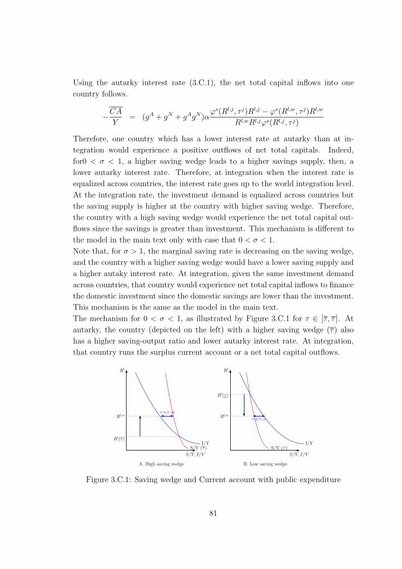
Using the autarky interest rate (3.C.1), the net total capital inflows into one
country follows.
−CAY
= (gA + gN + gAgN)αϕs(Rl,j, τ j)Rl,j − ϕs(Rl,w, τ j)Rl,w
Rl,wRl,jϕs(Rl,j, τ j)
Therefore, one country which has a lower interest rate at autarky than at in-
tegration would experience a positive outflows of net total capitals. Indeed,
for0 < σ < 1, a higher saving wedge leads to a higher savings supply, then, a
lower autarky interest rate. Therefore, at integration when the interest rate is
equalized across countries, the interest rate goes up to the world integration level.
At the integration rate, the investment demand is equalized across countries but
the saving supply is higher at the country with higher saving wedge. Therefore,
the country with a high saving wedge would experience the net total capital out-
flows since the savings is greater than investment. This mechanism is different to
the model in the main text only with case that 0 < σ < 1.
Note that, for σ > 1, the marginal saving rate is decreasing on the saving wedge,
and the country with a higher saving wedge would have a lower saving supply and
a higher autaky interest rate. At integration, given the same investment demand
across countries, that country would experience net total capital inflows to finance
the domestic investment since the domestic savings are lower than the investment.
This mechanism is the same as the model in the main text.
The mechanism for 0 < σ < 1, as illustrated by Figure 3.C.1 for τ ∈ [τ , τ ]. At
autarky, the country (depicted on the left) with a higher saving wedge (τ) also
has a higher saving-output ratio and lower autarky interest rate. At integration,
that country runs the surplus current account or a net total capital outflows.
S/Y, I/Y
Rl
S/Y (τ)I/Y
Rl(τ)
Rl,wCA/Y >0
S/Y, I/Y
Rl
S/Y (τ)I/Y
Rl(τ)
Rl,wCA/Y <0
A. High saving wedge B. Low saving wedge
Figure 3.C.1: Saving wedge and Current account with public expenditure
81

Chapter 4
Saving Wedge, Productivity
Growth and International Capital
Flows
Abstract
In one open OLG economy, the interaction of endogenous saving wedge and credit
constraint can explain the pattern of international capital flows for the emerg-
ing economies. A higher productivity growth rate leads to a higher saving by
raising the capital taxation and depressing the domestic interest rate. A lower
financial development level (tighter credit constraint) reduces the capital accumu-
lation in long run. Therefore, the emerging economies with the high productivity
growth and low financial development level can experience (1) the net total cap-
ital outflows; (2) the high saving-output ratio and (3) the low long-run capital
accumulation.
82

4.1 Introduction
The international financial integration of the emerging economies whose the high
output growth rates into the world economy for the last decades is featured by
three stylized facts.
Fact 1: The emerging economies experience the net total capital outflows (e.g,
China and Korea in Figure 4.1.1A). Furthermore, the value of net total capital
inflows fluctuates over time. The net total capital inflows for China has decreased
gradually to the bottom of −9% in 2007, then, it has increased again.
Fact 2: The emerging economies have the higher saving rates than the advanced
economies: on average, 40 % in China compared with 16 % in United States (Fig-
ure 4.1.1B). Moreover, the saving-output ratios increase substantially over time in
the emerging economies.
Fact 3: Some emerging economies have the persistently low capital-effective-labor
ratio than the advanced economies even after many years of integration: about
55000 USD in China compared with about 280000 USD in United States in 2013
(Figure 4.1.1C). Some economies, however, can converge to the same ratio with
the advance economies (in Korea, from 40000 USD in 1980 to 210000 USD in
2013).
The combination of the high saving rate and low capital accumulation in the capi-
tal exporters whose the high output growth rates (the fast-growing or the emerging
economies) raises the challenge for the existing theoretical models. Many models
can generate the high savings (fact 2) and low interest rate in the fast-growing
economies so that these economies experience the net capital outflows at integra-
tion (fact 1). These models, however, cannot account for the fact 3 since the high
saving also results in the high capital accumulation. Other models can depress
the investment demand on the fast-growing economies so that they converge to a
low long-run capital accumulation (fact 3) and export capital to the rest of world
(fact 1). These models, however, ignore the high saving rates on the emerging
economies (fact 2). In sum, there is still a research gap on the literature for the
explanation of these three facts simultaneously.
Our paper presents the theory of the endogenous financial friction to rationalize
these facts together. In the benchmark open OLG economy, the wedge between
the domestic interest rate on saving and the world rental rate of capital is increas-
ing on the domestic output growth rate. A higher growth rate not only increases
the investment but also the saving by raising the wedge and depressing the do-
mestic interest rate. Then, one economy which grows faster can experience the
83

outflows of net total capital if the saving increases faster than the investment.
Therefore, the benchmark model can account for the highly correlated between
the productivity growth and capital flows not only in the developing economies
but also in the advanced economies. In the extended economy with the credit
constraint (a measure of financial development level) for the domestic firms, the
capital accumulation is increasing on the tightness of the constraint. Therefore,
the heterogeneity on the tightness of the constraint generates the difference on
the long-run capital accumulation levels across countries. By combining the high
output growth rate and low financial development level, our model can explain
the high saving rate (fact 2) and low capital accumulation (fact 3) in the emerging
economies who export the capital to the rest of world (fact 1).
The paper belongs to the literature on the international capital flows (see ? for a
recent survey). Some papers focus on the transition economies by employing one
small open economy which takes the interest rate as exogenous given. Buera and
Shin (2009) analyze the large-scale reforms which reduce the financial friction on
investment and improve the contract’s enforcement in one small open economy.
The reform raises the productivity growth by a more efficient allocation of eco-
nomic resources and at the same time, it also results in the outflows of net total
capital since the saving rate surges but the investment rate increases with lag.
The financial friction is endogenous determined by the productivity growth rate
in our model while the productivity growth is endogenously determined by the
financial frictions in their model. Therefore, the capital outflows is driven by the
productivity growth in our model, instead of the reduction of the financial friction
as theirs.
Song, Storesletten and Zilibotti (2011) also explain the high productivity growth
rate and capital outflows in an transition economy like China with two types of
firms: the entrepreneurial firms with the high productivity level but credit con-
straint and the financial firms with the low productivity level with the abundant
finance. The reform in term of moving of labor force from the financial to en-
trepreneurial firms raises the wage rates and the aggregate savings through the
wealth effect. This reform also results in the net total capital outflows since the
aggregate savings increase while aggregate investments decrease because of the re-
duction of investment demand by the financial firms. Instead of aggregate savings,
our model focuses on the change in the marginal saving rate as the driving force
of the increasing savings-output ratio and the net capital outflows.
None of two aformentioned papers accounts for the non-convergence of the emerg-
ing economies toward the long-run capital accumulation levels of advanced economies.
84

Figure 4.1.1: Three Stylized Facts
Notes: (a) Net total inflows (negative Current account) per Output; (b) Aggregate
savings is the sum of private and public savings; both (a) and (b) are from Alfaro,
Kalemli-Ozcan and Volosovych (2014); (c) Capital-effective-labor ratio equals to capital
stock at constant 2005 national prices (in millions USD) divided by total effective units
of labor, which is the productivity level at constant 2005 national prices multiplied by
number of people engaged (in millions). Data from PWT 8.1
85

In comparison with their model, ours captures the increasing saving-output ratio
(fact 2) while still explains the outflows of net total capital from the emerging
economies (fact 1).
Some papers endogenize the interest rate by building up the multi-country econ-
omy. On Coeurdacier, Guibaud and Jin (2015), the borrowing constraint, which is
more severe in the developing economies than in the advanced economies, generates
the excess savings and low interest rate in the developing economies at autarky.
Then, at integration, the capital flows out of these economies for a higher interest
rate in the advanced economies. The high saving and low interest rate at autarky
economy are also the key implications on Angeletos and Panousi (2011) where
the idiosyncratic investment risk motivates the precautionary savings by house-
holds. The common mechanism on these model is that the developing economies
have a higher capital accumulation and a lower interest rate at autarky than the
advanced economies. At integration, the capital flows from the developing to ad-
vanced economies to equalize the capital accumulation and the interest rate across
countries. This implication is inconsistent to the fact 3 that the some developing
economies could not converge to the same long-run capital accumulation with the
advanced economies even at integration.
Other multi-country models focus on the investment demand as the driver of in-
ternational capital flows. On Boyd and Smith (1997), the rich economy has a
higher investment demand since it has much more income than the poor one to
afford the agency cost on the financial market. Therefore, the capital flows out
from the developing economies to the advanced economies for a higher investment
demand. The difference in the investment demand across countries is also the
key feature on Matsuyama (2004) in which two economies face the same credit
constraint converge to asymmetric steady states because of the difference on the
initial capital stock. Indeed, the capital flows from the poor to the rich economy
since the latter has a higher steady state capital accumulation. These two papers,
however, do not account for the fact 2 that the exporters of capital also have the
high saving-output ratios.
There are two key features that distinguishes our paper to these multi-country
models. First, our model can explain simultaneously the high saving-output ratio
and low capital accumulation on the emerging economies who export the capital
to the rest of world. Second, while the financial friction is exogenous in the afore-
mentioned papers, it is endogenously determined by the productivity growth rate
in our model. Therefore, the net total capital inflows can fluctuate over time as
presented in Firgure 4.1.1.A.
86

The paper is related to the literature on the puzzling high correlation between
saving and investment on the open economy (Feldstein and Horioka (1979)). On
Carroll, Overland and Weil (2000), the utility depends partly on how consump-
tion compares to a habit stock determined by past consumption. Therefore, an
increase on the output growth rate can cause an increase on the saving rate by lim-
iting the motive of consumption smoothing. In stead of using the habit formation,
Kraay and Ventura (2000) employ the classical Merton-Samuelson portfolio choice
approach to the current account. On their model, the agent with CRRA utility
function would allocate the constant fraction of wealth between the riskfree and
risky assets. Therefore, a positive income shock can raises both the wealth accu-
mulation growth rate (saving) and the portfolio investment. Our model, however,
employs one endogenous saving wedge to explain the high correlation between sav-
ing and investment. This key opens the channel through which the output growth
affects both the saving and investment rates. Indeed, a high output growth rate
raises the investment to keep the domestic marginal product of capital to be equal
to the world rental rate of capital. Moreover, a higher growth rate raises the sav-
ing by depressing the domestic rate of return on the saving. Therefore, both the
saving and investment go up for a higher growth rate.
The paper also makes contribution on the literature on interest rate spread, such
as Campbell and Shiller (1991), Bernanke and Blinder (1992),Ho and Saunders
(1981). Our different position is to emphasize the capital taxation as the key to
create the gap between lending interest rate for the firms and the deposit interest
rate for the households. Since the government collects tax to finance a public ex-
penditure which is complementary to private output, an increase of future output
growth rate raises the tax rate and widens the interest rate spread. Therefore, the
future output growth rate is an important predictor for the interest rate spread,
not vice versa like the rest of literature.
The paper is organized as follows. After the introduction, section 4.2 provides
the definition of interest rate wedge and the empirical analysis on the relation-
ship between productivity growth and international capital flows. Section 4.3 and
4.4 lay out the theoretical models to explain the empirical evidence. Section 4.5
concludes and is followed by Appendix.
4.2 Saving wedge: Definition
Gourinchas and Jeanne (2013) define the saving wedge as the difference between
the domestic interest rate (Rj) and world interest rate (Rw) which is exogenous
87

for one small open economy j.
Rj = (1− wedgej)Rw
They calibrate the wedge such that the net total capital flows predicted by model
fit the cross-section data sample of Non-OECD countries. The result is that the
wedge is higher in African economies and lower for emerging Asian economies
(for instance, China and Korea): countries with low productivity growth rate
tax saving while countries with high productivity growth rate subsidy saving.
Moreover, the wedge is decreasing on the level of financial development and on
the income per capita.
The saving wedge can be one type of financial friction that creates the gap between
the rental rate of capital for domestic firms (which equals to world interest rate
for one small open economy without credit constraint) and the rate of return on
savings for households. Since there does not exist one world lending interest rate
across countries, we can not compute the exact measure of saving wedge by data.
In fact, we can only observe the deposit interest rate (Rd,jt ) which is the rate of
return on saving and the lending interest rate (Rl,jt ) which is the cost of capital in
one country j at time t. Then, we define the wedge as the relative gap between
the lending and deposit interest rates.
wedgejt ≡Rl,jt −R
d,jt
Rl,jt
On the theoretical ground, the wedge, as one type of financial friction, should be
decreasing on output growth rate and on the income levels. Indeed, one country
with the high economic growth or income level can be affordable to finance a better
but costly financial system (Lucas (1988), Greenwood and Jovanovic (1990)) or
better institutional quality (Levine, Loayza and Beck (2000), Rajan and Zingales
(1998)). A higher level of financial development can, in turn, reduce the financial
friction level, such as the cost induced by the asymmetric information like state-
verifying cost, agency cost (Hubbard (1998), Gertler and Rogoff (1990),Bernanke
and Gertler (1989)). Moreover, a higher level financial development can push up
the economic growth an efficient allocation of the capital to the most productive
project (Beck and Levine (2004), King and Levine (1993)). To sum up, the theory
suggests that, on controlling for the level of financial development, the economic
growth and income level should have negative impacts on the saving wedge.
88

4.3 Empirical evidences
We carry out the empirical tests for a sample of 169 countries from 1980 to 2013.
The objective is to use the saving wedge and the financial development level to
shed the new lights on the relationship between the productivity growth rate and
the net total capital inflows. We perform the fixed-effect panel data analysis
to capture the pattern of capital inflows over time and also to control for the
unobserved heterogeneity which is constant over time in each country.
Productivity growth and International capital flows: the role of saving
wedge
Table 4.3.1: Fixed-effect estimation results of saving wedge: 1980-2013.
(1) (2) (3)
VARIABLES wedge wedge wedge
Time trend (t) 0.0137*** 0.0118*** 0.0118***
(0.000498) (0.000368) (0.000383)
Financial development level (FinDev) -0.00143*** -0.00155*** -0.00156***
(0.000204) (0.000183) (0.000178)
Openness (kaopen) 0.0148*** 0.0234*** 0.0162***
(0.00372) (0.00303) (0.00312)
Productivity growth rate (TFPgrowth) 0.00239***
(0.000805)
Output-per-capita growth rate (GDPpcgrowth) 0.000847*
(0.000486)
Output (GDP ) 3.03e-08***
(6.84e-09)
Constant -26.85*** -23.12*** -23.08***
(0.990) (0.732) (0.762)
Observations 2,191 3,722 3,232
R-squared 0.356 0.307 0.316
Number of countries 99 161 145
Note: standard errors in parentheses. *** p<0.01, ** p<0.05, * p<0.1. (wedge) is the saving
wedge; (FinDev) is the financial development level measured by domestic credit to private
sector; (kaopen) is the Chinn-Ito index of openness; (TFPgrowth) is the productivity growth
rate; (GDPpcgrowth) is the output-per-capita growth rate and (GDP ) is the output measured
as Gross Domestic Product. Productivity is at constant national prices (2005=1). Output is
the real GDP at constant 2005 national prices (in mil. 2005USD). Output-per-capita is the
real GDP at constant 2005 national prices (in mil. 2005USD) per number of persons engaged
(in millions).
Table 4.3.1 investigates the determinants of the interest rate wedge. In all these
columns, the wedge is decreasing on the level of financial development, a confir-
mation that the wedge can illustrate for the level of financial friction. Column
1 shows that the wedge is increasing on the productivity growth. Column 2 and
column 3 demonstrate that the wedge is still increasing on the output-per-capita
89

Table 4.3.2: Fixed-effect estimation results of the net total capital inflows: 1980 -
2013.
(1) (2) (3) (4)
VARIABLES annual negCA2y ifs annual negCA2y ifs annual negCApc ifs annual negCApc ifs
Time trend (t) -0.0942*** -0.0664*** -7.816*** -11.28***
(0.0167) (0.0201) (1.760) (2.484)
Saving wedge (wedge) -4.461*** -278.2**
(0.831) (109.5)
Productivity growth rate (TFPgrowth) -0.250*** -1.025
(3.452) (3.252)
Output growth rate (GDPgrowth) -14.48*** -97.77
(320.4) (372.4)
Constant 190.1*** 136.0*** 15,588*** 22,550***
(33.32) (40.02) (3,512) (4,934)
Observations 2,934 2,219 4,237 3,172
R-squared 0.031 0.040 0.011 0.018
Number of countries 109 103 162 151
Note: standard errors in parentheses. *** p<0.01, ** p<0.05, * p<0.1. Two alternative measures of the annual net total capital
inflows: one as the ratio over GDP (negCA2y ifs) and other as the ratio over Population (negCApc ifs); (TFPgrowth) is
the productivity growth rate; (GDPgrowth) is the output growth rate. Productivity is at constant national prices (2005=1).
Output is the real GDP at constant 2005 national prices (in mil. 2005USD).
growth rate and the output level. These results prove that the direct impact of
economic growth rate on the saving wedge is positive, on controlling for the level
of financial development.
The positive dependence of the wedge on the productivity growth rate is contra-
dicted to the prediction by theory on the financial friction. This puzzling fact,
however, does not reject that the wedge is one type of financial friction but only
reveals that the wedge can contain other indicators which are positively dependent
on the productivity growth.
Since a higher productivity growth rate raises the saving wedge, we can expect
the wedge to be one channel for the growth rate to affect the savings and then
the net total capital inflows. Following Alfaro, KalemliOzcan, and Volosovych
(2008), the strategy is to add the saving wedge into the regression of the net total
capital inflows on the productivity growth rate. If the coefficient of the productiv-
ity growth rate turns to be insignificant, we conclude that the saving wedge can
account for the impact of the productivity growth on the net total capital inflows.
We employ this strategy in the next regression.
Table 4.3.2 shows the role of the saving wedge on solving the puzzling positive
relationship between the net total capital inflows and the productivity growth
rate (Allocation puzzle). Column 1 shows that the 1 % of increase on the pro-
ductivity growth rate reduces 0.25 % of the net total capital inflows: one country
90

Table 4.3.3: Fixed-effect estimation results of output-effective-labor ratio (K2AL)
and capital-effective-labor ratio (Y 2AL).
(1) (2) (3) (4)
VARIABLES K2AL K2AL Y2AL Y2AL
Time trend (t) 955.6*** 545.5*** 338.4*** 227.3***
(51.72) (95.27) (12.34) (21.23)
Financial development level (FinDev) 206.3*** 218.9*** 43.27*** 53.55***
(20.66) (19.32) (4.929) (4.306)
Productivity growth rate (TFPgrowth) -614.2*** -490.1*** -92.95*** -63.84***
(8,806) (8,206) (2,101) (1,829)
Human capital 24,001*** 5,190***
(4,175) (930.4)
Government size 639.8*** -149.3***
(124.3) (27.71)
Constant -1.821e+06*** -1.073e+06*** -644,000*** -433,236***
(102,764) (181,256) (24,518) (40,391)
Observations 3,008 2,973 3,008 2,973
R-squared 0.229 0.282 0.328 0.407
Number of countries 109 109 109 109
Note: robust standard errors in parentheses. *** p<0.01, ** p<0.05, * p<0.1. (Y 2AL) is the output-
effective-labor ratio and (K2AL) is the capital-effective-labor ratio; (FinDev) is the financial devel-
opment measured by domestic credit to private sector; (TFPgrowth) is the productivity growth rate;
Human capital is the index of human capital per person; Government size is the public expenditure
per output ratio. Capital-effective-labor ratio equals to capital stock at constant 2005 national prices
(in million USD) divided by total effective units of labor, which is the productivity level at constant
2005 national prices multiplied by number of people engaged. Output-effective-labor ratio equals to
GDP at constant 2005 national prices (in million USD) divided by total effective units of labor.
which grows faster tends to export the capital to the rest of world. Column 2
demonstrates that the addition of the saving wedge makes the coefficient of the
productivity growth to be insignificant. And, a higher saving wedge reduces the
net total capital inflows. Therefore, the regression results prove that the saving
wedge is crucial to explain the allocation puzzle. Column 3 and 4 repeat the same
exercise for the other measures of net total capital inflows and economic growth.
The increase of 1 % on the output growth rate raises 14.48 % of net total capital
outflows per capita. Adding the saving wedge, however, makes the coefficient of
output growth rate to be insignificant. And the wedge has a significantly negative
impact on the net total capital inflows. Therefore, the regression also supports
the important role of the saving wedge on solving the Allocation puzzle.
Capital accumulation: the role of financial development
Table 4.3.3 examines the role of financial development on determining the capi-
tal accumulation. Column 1 shows that a higher level of financial development
increases the long-run capital accumulation, as measured by the capital-effective-
91

labor ratio. Column 2 demonstrates that the result is maintained when we control
for the productivity growth rate, the government’ size and the human capital 1.
Column 3 and 4 prove that a higher financial development level also raises the
output-effective-labor ratio, even controlling for the government’s size and the hu-
man capital. On short, the financial development level has a positive impact on
the long-run capital accumulation and output.
We summarize the empirical evidence as three stylized facts:
1. The saving wedge is increasing on the productivity growth rate. This puz-
zling fact reveals that the wedge contains the variable which is increasing on
the productivity growth.
2. The saving wedge is an important channel for productivity growth rate to
affect the cross-border capital flows.
3. The long-run capital accumulation is increasing on the financial development
level.
In the next section, we develop one benchmark model of the international capital
flows based on the endogenous saving wedge to be consistent with the first two
empirical stylized facts. Indeed, we will show that in one country, an increase
of productivity growth can raise the net total capital outflows. On the extended
economy, we add the credit constraint for firms as the measure of financial devel-
opment level to explain the long-run capital accumulation. Then, we will show
that the capital can flows out of the country with the high productivity growth
rate and low capital-effective-labor ratio.
4.4 Benchmark Model: Productivity growth and
International capital flows
The model is one small open economy which take the world interest rate as ex-
ogenous given. There is one homogeneous good, which is used for consumption
and investment, and is traded freely and costlessly. Capital is free mobile between
the country and the rest of world but labor is immobile, and firms are subject to
changes in the productivity and labor force.
1Levine, Loayza and Beck (2000a, b) find that the human capital and government size have
positive impact on capital accumulation and output
92

Specification of the thereotical model
The theoretical model is constructed to be consistent with the empirical evidences,
which are based on a panel-data yearly sample for 160 economies. The time
dimension on the panel sample allows us to study the dynamics of the dependence
pattern of capital flows on the productivity growth over time. And the cross-
section dimension on the panel sample helps us to capture the common pattern
of capital flows among the different countries. These two features are both taken
into account on the construction of the theoretical model.
The theoretical model is one small open OLG economy which takes the interest
rate as exogenous given by the world capital market. With the exogenous interest
rate, the model is ready to capture the dynamics of the interested variables over
time, such as the saving and investment rates. This approach is also employed
by Gourinchas and Jeanne (2013) to analyze the pattern of capital flows on the
productivity growth rate. Moreover, the heterogenous agents (young and old)
of OLG helps us to focus on the distortion induced by the capital taxation on
the marginal saving rate. Indeed, since an agent only lives for two period, the
future income become unplegible. Therefore, she can not use the future incomes
by the incomming young agents to smooth her consumption, one key mechanism
in the Ramsey representative agent framework. On other word, the Ricardian
equivalence on the unrelevant timming of taxation does not hold on our model.
In sum, the small open OLG model is appropriate to analyze role of the capital
taxation on shaping the pattern of capital flows on the productivity growth.
There is also a problem with the OGL framework. In details, the model is not
a perfect replication of the yearly time series. Indeed, since each agent lives for
two periods (young and old), each time period is appropriated of 30 years in the
real life time. This structure is at odd with the yearly frequency on our data
sample. Althouth a multi-period OLG economy can capture this time frequency,
the cost is that we need to rely on the numerical solution rather than an analytical
solution in the two-period OLG economy. Therefore, by comparing between the
benefits and cost of an small open OLG model, we conclude that the model is still
a convenient framework to capture the dynamic pattern of capital flows on the
productivity growth.
Furthermore, the small open economy can be an easy way to approach the large
open economy. Indeed, the analysis of one large open economy is in the middle
between one closed economy (which fully affect the world equilibrium) and one
small open economy (which can not affect the world equilibrium). Therefore, using
one small open economy to analyze the case of large economy will miss the partial
93

effect of that economy on the world equilibrium. The advantage, however, is one
tractable framework which helps us to focus on the other endogenous variables
rather than the equilibrium interest rate. This approach is employed by Song,
Storesletten and Zilibotti (2011) for one small open economy version of China.
In sum, the small open economy in our theory can be an appropriate set-up to
capture the pattern of capital flows for a sample of many economies although we
admitedly can not capture fully this pattern.
4.4.1 Production
The domestic output is produced by one representative firm which employs the
capital (Kt) and labor (Nt) with the constant-return-scale technology.
Yt = Kαt (AtNt)
(1−α)gηt (4.4.1)
The production function is a la Barro and Sala-I-Martin (2002) in which the
public expenditure (gt) is one type of production factor. In details, gt =Gt
AtNt
,
whereby Gt is the public expenditure.
Let’s define κt =Kt
Nt
as the capital-labor ratio and κt =Kt
AtNt
as the capital-
effective-labor ratio. Then, the output-effective-labor ratio is:
yt ≡YtAtNt
= καt gηt (4.4.2)
The profit maximization problem for the firm facing the world exogenous interest
rate (Rw) and the wage rate (wt) is as following:
Πt = Kαt (AtNt)
(1−α)gηt −RwKt − wtNt (4.4.3)
With depreciation rate (0 < δ < 1), the law of motion for capital follows:
Kt = It + (1− δ)Kt−1 (4.4.4)
With the perfect market for factor of production, the interest rate equals to the
marginal product of capital.
Rw = ακ(α−1)t gηt (4.4.5)
Therefore, the economy’s total demand for capital takes the form:
K(Rw, At, Nt) = AtNtκt = AtNt
( α
Rw
)1/(1−α)
gη/(1−α)t (4.4.6)
94

and the corresponding real wage is equal to the marginal product of labor:
wt = (1− α)At
( α
Rw
)α/(1−α)
gη/(1−α)t (4.4.7)
Plugging (4.4.6) into (4.4.1), the output is:
Yt = AtNt
( α
Rw
)α/(1−α)
gη/(1−α)t (4.4.8)
4.4.2 Consumption
There are Nt newborn agents at t, each supplies one unit of labor at young and
retires at old. Let denote (cyt , syt ) as the consumption and saving by the young
agent at t and (cot+1) as the consumption by that agent at old.
The utility maximization problem is:
max(cyt ,cot+1,s
yt )u(cyt ) + βu(cot+1)
cyt + syt = wt
cot+1 = Rwsyt − tt+1
Whereby the utility function u(c) =c1−1/σ
1− 1/σwith the inter-temporal elasticity
of substitution coefficient σ and the discount factor satisfies 0 < β < 1. We will
focus on the case that (0 < σ < 1) which implies that the income effect dominates
the substitution effect. This range of value is consistent with literature on asset
pricing (Guvenen (2006) for one discussion) and many empirical papers (Hall
(1988), Ogaki and Reinhart (1998)) which estimate the coefficient of substitution
below 1.
The tt+1 is the capital taxation levied by the government. We assume that the
government follows the residence principle in taxation: tax based on where the
agents live, no matter the source of income is from the domestic or foreign markets.
We also impose that the taxation is proportional to the capital income:
tt+1 = τt+1Rwsyt (4.4.9)
The Euler equation is:
u′(cyt ) = βRw(1− τt+1)u′(cot+1)
Therefore, the capital taxation affects the marginal saving rate:
syt = ϕs(τt+1)wt (4.4.10)
95

where we define the marginal saving rate
ϕs(τt+1) ≡ 1
1 + β−σ[Rw(1− τt+1)](1−σ)
For 0 < σ < 1, the marginal saving rate is increasing on the capital taxation (i.e,
∂ϕ(τt+1)/∂τt+1 > 0) since a higher tax reduces the rate of return on the savings,
then raises the marginal saving rate.
4.4.3 Government
As on Barro and Sala-I-Martin (2002), the government demands for the public
good such that its marginal product of expenditure (∂Yt/∂Gt) equals to its price,
which is 1.
Gt = ηYt (4.4.11)
In order to finance the public expenditure, the government levies the capital tax-
ation:
Tt = τtRwNt−1s
yt−1
We assume that the government always keeps the balanced budget2.
τtRwNt−1s
yt−1 = ηYt (4.4.12)
Replacing (4.4.7) into (4.4.10), and the result into (4.4.12), we get an equation
determining the endogenous capital taxation:
τtRwϕs(τt) =
η
(1− α)
YtYt−1
(4.4.13)
Therefore, by the implicit function theorem, the capital taxation is increasing on
the output growth rate.∂τt
∂(Yt/Yt−1)> 0
Since the public expenditure is complementary to the private output, a higher
output growth rate raises the demand for the public expenditure. With a balanced
budget constraint, the government needs to raises the capital taxation.
2The balanced government’s budget constraint differs our theory to the literature on inter-
national taxation where government involves in debt and has to issue the bond and increase tax
to finance public debt
96

4.4.4 Equilibrium
Plugging the public expenditure (4.4.11) into (4.4.8), the output is:
Yt =( α
Rw
)α/(1−(α+η))
ηη/(1−(α+η))AtNt (4.4.14)
Taking into account that (4.4.11) implies gt = ηyt and using (4.4.5), we have the
capital-effective-labor ratio:
κ =( α
Rw
)(1−η)/(1−(α+η))
ηη/(1−(α+η)) (4.4.15)
Therefore, the demand for capital is as following:
Kt = κtAtNt =( α
Rw
)(1−η)/(1−(α+η))
ηη/(1−(α+η))AtNt (4.4.16)
Finally, replacing (4.4.11) into (4.4.7), the wage rate is:
wt = (1− α)( α
Rw
)α/(1−(α+η))
ηη/(1−(α+η))At (4.4.17)
4.4.5 International capital flows
With the productivity and labor force growth rates, the steady state is constructed
by scaling all key variables by output.
Dividing (4.4.16) by (4.4.14), the capital-output ratio is:
Kt
Yt=
α
Rw(4.4.18)
Plug (4.4.18) into (4.4.4) and scaling by the output, we end up with the share of
investment in current output.
ItYt
=Kt+1
Yt+1
Yt+1
Yt− (1− δ)Kt
Yt
By (4.4.14), the output growth rate is as following.
Yt+1
Yt= (1 + gAt+1)(1 + gNt+1) (4.4.19)
Therefore, we end up with:
ItYt
=[(1 + gAt+1)(1 + gNt+1)− 1 + δ
] α
Rw(4.4.20)
97

The investment-output ratio is increasing on the productivity and labor force
growth rates since they raise the demand for capital to keep the marginal product
of capital to be equal to the world exogenous interest rate. It is decreasing on the
interest rate since the latter is the cost of capital for domestic firms.
Using the solution for the wage in (4.4.17) and the assumption of zero earning in
old age, a typical date t young agent saves the amount.
syt = (1− α)( α
Rw
)α/(1−(α+η))
ηη/(1−(α+η))Atϕs(τt+1) (4.4.21)
Let denote (Syt , Sot ) as the stocks of the aggregate savings by the young and old
agents at the end of t. Since sot = −syt−1, we have:
Syt ≡ Ntsyt = (1− α)ϕs(τt+1)Yt
Sot ≡ Nt−1sot = (1− α)ϕs(τt)Yt−1
The stock of the aggregate savings (St) at the end of t is the sum of the savings
by the young and old agents.
StYt
=Nts
yt −Nt−1s
yt−1
Yt= (1− α)ϕs(τt+1)− (1− α)ϕs(τt)
(1 + gAt )(1 + gNt )(4.4.22)
The saving-output ratio depends on the expected productivity and labor force
growth rates through the capital taxation. Indeed, a higher growth rate raises the
capital tax rate and depresses the domestic rate of return on saving. Therefore,
for 0 < σ < 1, a higher future productivity growth rate raises the marginal saving
rate by the young agents.
The saving of the young has two components, net foreign assets (Bt+1) and the
capital stock that will be used in the production in the next period.
Syt = Bt+1 +Kt+1 (4.4.23)
Therefore, by using (4.4.21), (4.4.19) and (4.4.18), the net stock of foreign assets,
measured as a fraction of output, is:
Bt+1
Yt+1
=SytYt
YtYt+1
− Kt+1
Yt+1
=(1− α)ϕs(τt+1)
(1 + gAt+1)(1 + gNt+1)− α
Rw(4.4.24)
The current account is the change in the net stock of foreign assets .
CAtYt
=Bt+1
Yt+1
Yt+1
Yt− Bt
Yt(4.4.25)
98

At steady state of constant productivity and labor force growth rates (gA, gN), the
output growth rate is constant, then by (4.4.13),the capital tax rate is constant
(τt = τt+1 = τ). Moreover, all key variables scaled by the total effective units of
labor are constant. Therefore, the steady-state net foreign assets at the beginning
of period is:B
Y=
(1− α)ϕs(τ)
(1 + gA)(1 + gN)− α
Rw(4.4.26)
Replacing (4.4.26) into (4.4.25), the steady-state current account to finance the
net foreign assets is as following.
CA
Y= (gA + gN + gAgN)
B
Y(4.4.27)
To analyze the impact of an increase on the productivity growth rate, we assume
that the economy has an initial zero net foreign assets position at the productivity
growth rate (gA,∗), that isCA
Y(gA,∗) =
B
Y(gA,∗) = 0. Then, we carry out the
Taylor expansion to get the net total capital inflows (measured by the negative
current account) for an increase of the productivity growth rate from gA,∗ to gA.
− CA
Y(gA) ≈ ∂(−CA/Y )
∂gA|gA,∗ (gA − gA,∗) (4.4.28)
By taking into account the dependence of the marginal saving rate on the produc-
tivity growth rate through the capital taxation, the change of the net total capital
inflows is:
∂(−CA/Y )
∂gA|gA,∗= (gA,∗ + gN + gA,∗gN)
∂(−B/Y )
∂gA|gA,∗ (4.4.29)
Therefore, all the change in the net total capital inflows are from the change in
the net foreign asset stock.
∂(−B/Y )
∂gA|gA,∗ =
(1− α)
(1 + gA,∗)(1 + gN)
ϕs
gA,∗
[gA,∗
(1 + gA,∗)− εϕ
gA,∗
](4.4.30)
Where we define the elasticity coefficient of the marginal saving rate by the young
agent w.r.t the productivity growth rate as: εϕgA,∗≡ ∂ϕs
∂gA,∗gA,∗
ϕs. For 0 < σ < 1,
∂ϕs
∂gA,∗> 0 and therefore, εϕ
gA,∗> 0.
Placing (4.4.30) into (4.4.29), then the result into 4.4.28, we end up with:
− CA
Y(gA) =
(gA,∗ + gN + gA,∗gN)
(1 + gA,∗)(1 + gN)
(1− α)ϕs
gA,∗
[gA,∗
(1 + gA,∗)− εϕ
gA,∗
](gA − gA,∗)
(4.4.31)
99

A higher productivity growth rate has two effects that tends to offset each other.
The traditional channel is that a higher growth rate reduces the share of the
saving by current young agents over the following period’s output. Indeed, a
higher productivity growth rate leads to a higher investment demand to keep the
marginal product of capital to be equal to the world exogenous rental rate of
capital. Given the share of savings by current young agents over current output,
a higher productivity growth rate makes the saving by current young agents to
be not enough for a higher investment demand. Therefore, the country needs to
borrow from the rest of world to finance the increase of investment demand. We
label this effect as the Neo-Classical growth effect, which implies that one country
growing faster would experience net capital inflows to finance domestic investment,
given the domestic saving is unaffected by the growth rate.
One new channel emerges within our model with the endogenous saving wedge. A
higher productivity growth rate raises the share of the savings by current young
agents over the current output. Since the public expenditure is complementary
to the the private output, a higher growth rate requires the government to raise
the capital taxation in order to finance a higher public expenditure. A higher tax
rate, in turn, depresses the domestic interest rate and raises the marginal saving
rate for the low value of the inter-temporal substitution coefficient. Therefore, the
savings by the young agents goes up. Given the investment demand, the country
lends the capital, which is dued to the increase of savings, to the rest of world.
We label this effect as the saving-wedge effect.
The impact of an increase of the productivity growth rate on the net total capital
inflows depends on the relative magnitude of the Neo-Classical growth effect and
the saving-wedge effect, which is summarized on the following proposition.
Proposition 4.4.1. Suppose that the net foreign assets is zero at the initial pro-
ductivity growth rate gA,∗. At a higher productivity growth gA > gA,∗, the net total
capital inflows is positive if εϕgA,∗
<gA,∗
(1 + gA,∗)and negative if εϕ
gA,∗>
gA,∗
(1 + gA,∗).
Proof. The result is implied directly by the equation (4.4.31). �
Note that since a higher productivity growth raises both the saving and investment
rates, the threshold on the elasticity coefficient of marginal saving rate is increasing
on the initial productivity growth rate:gA,∗
1 + gA,∗. Indeed, the condition that
εϕgA,∗
>gA,∗
1 + gA,∗implicitly implies that the saving raises more than the investment.
Moreover, without the endogenous saving wedge (εϕgA,∗
= 0), a higher productivity
100

growth only raises the investment rate, and then an increase on the inflows of
capital.
S/Y, I/Y
R
S/Y I/Y (gA,∗) I/Y (gA)
CA/Y < 0Rw
S/Y, I/Y
R
S/Y (gA,∗)S/Y (gA)
I/Y (gA,∗) I/Y (gA)
CA/Y > 0Rw
A. Without endogenous wedge B. With endogenous wedge
Figure 4.4.1: Saving wedge and Current account
Figure 4.4.1 demonstrates the role of the endogenous saving wedge on shaping the
pattern of the international capital flows, given the initial zero capital flows. On
panel A, the saving-output ratio is independent on the productivity growth rate.
A higher growth rate raises the investment demand by shifting the investment
curve to the right. The current account turns to be deficit. On panel B, the
saving-output ratio depends on the productivity growth rate. A higher growth
rate not only shifts to the right the investment curve (Neo-Classical growth effect)
but also the saving curve (Saving-wedge effect). If εϕgA> gA,∗/(1 + gA,∗), the sav-
ing curve moves further than the investment curve, the current account turns to
be surplus. Therefore, one fast-growing economy still experiences the outflows of
net total capital if the saving-wedge effect overshadows the Neo-Classical growth
effect.
Our theory justifies the empirical evidence that a higher growth rate can lead to
an increase of the net total capital outflows. Indeed, a higher growth rate raises
the investment demand like the prediction by the Neo-Classical growth model. A
higher productivity growth rate can also raises the saving by raising the capital
tax rate and depresses the rate of return on saving. If the saving supply increases
more than the investment demand, the fast-growing economy experiences an in-
crease of net total capital outflows.
The endogenous saving wedge is the key channel through which the productivity
growth rate can affect both the savings and the net total capital inflows. The
101

saving rate is increasing on the productivity growth since the intertemporal elas-
ticity of substitution coefficient is lower than 1. Coeurdacier, Guibaud and Jin
(2015) also employ this range of value to prove the outflows of capital from the
fast-growing economies with a tight credit constraint for the households.
Since the productivity growth raises both the saving and investment rates, our
model can account for the high correlation between the productivity growth rate
and the net total capital inflows over time. Figure 4.4.2 illustrates the case of
China and United States in which the fluctuation of the productivity growth rate
can be the predictor of the net total capital inflows. In China, the positive cor-
relation between the productivity growth and current account is clear over period
1995-2013. In United States, this positive co-movement pattern also appears for
some periods of time, such as 1983-1989, or 2007-2013.
Figure 4.4.2: Net total capital outflows and Productivity growth.
Notes: (a) TFPgrowth is gross growth rate of productivity level at constant national prices (2005=1). Data
from PWT 8.1; (b) Current account per GDP ratio from Alfaro, KalemliOzcan, and Volosovych (2015).
The benchmark model can explain the dependence pattern of international capital
flows on the productivity growth for both the advanced and developing economies.
In the next section, we employ the endogenous saving wedge to focus on the pattern
of net total capital outflows from the fast-growing country with the low long-run
capital accumulation.
4.5 Long-run capital accumulation
We add the credit constraint for the firms in the benchmark model to analyze
the role of financial development on the long-run capital accumulation. Only the
102

profit maximization problem for the firms is different to the benchmark model.
Production
The representative firm faces the credit constraint so that the total value of capital
stock can not excess a constant fration of output.
RwKt ≤ θYt (4.5.1)
The tightness of the parameter θ measures the financial development level as in
Song, Storesletten and Zilibotti (2011). Indeed, a higher θ illustrates for a better
financial system in which there are more financial resources for the domestic firms
to satisfy their investment demands.
We rewrite the profit maximization for the firms as:
Πt = Yt −RwKt − wtNt (4.5.2)
st : RwKt ≤ θYt (4.5.3)
Let denotes λt as the Lagrange multiplier for the credit constraint. With the bind-
ing credit constraint, the domestic firms can not satisfy their investment demand.
Therefore, the marginal product of capital is greater or at least equal to the world
interest rate as the cost of capital:
λt ≥ 0;∂Yt∂Kt
≥ Rw (4.5.4)
As the benchmark model, the government chooses the public expenditure to max-
imize the domestic output. Then, the public expenditutre constributes a constant
fraction of output: Gt = ηYt. Therefore, the output is3 :
Yt = (Kt)α(AtNt)
(1−α)gηt = ηη/(1−η)(κt)α/(1−η)AtNt (4.5.5)
Low capital-effective-labor ratio in long run
We will focus on the case of binding credit constraint. In fact, the constraint
would bind for a low value of financial development level (θ) or a high demand of
investment (KDt ) or a combination of both of these two features. By assuming the
binding credit constraint, we want to characterize the developing economies with
the low financial development levels and the high capital demands because of the
domestic scarcity of capitals.
3yt = (κt)α(gt)
η = (κt)α(ηyt)
η ⇒ y = (κt)α/(1−η)η(η/(1−η)). Then, Yt = ytAtNt
103

The binding credit constraint implies that: Kt =θ
RwYt. Dividing both sides by
AtNt, we have:
κt =θ
Rwyt (4.5.6)
Plugging (4.5.5) into the last equation, we get the capital-effective-labor ratio at
binding credit constraint is as following:
κb =
(θ
Rw
) (1− η)
1− (α + η)η
η
1− (α + η) (4.5.7)
The long-run capital accumulation with the binding constraint is decreasing on the
world lending interest rate since the latter is the cost of capital for the domestic
firms. It is increasing on the financial development level since the latter allows the
domestic firms to borrow more to build up the domestic capital stock.
The rest of world is assumed to include the advanced economies with a very high
level of financial development such that the credit constraint never binds. Then,
its capital-effective-labor ratio in long run is determined such that the marginal
product of capital equates the world lending interest rate. Moreover, we allow
that the rest of world’s production fuction can have a different share of capital:
αw ≥ α. By using 4.4.15, we have:
κw =
(αw
Rw
) (1− η)
1− (αw + η)η
η
1− (αw + η) (4.5.8)
On the next step, we can find one condition on the parameter θ so that one small
open economy would have a lower capital-effective-labor ratio in long run than the
rest of world, even when the capital is free mobile.
κb ≤ κw ⇔ θ ≤ θ ≡ (Rw)
α− αw
1− (αw + η) (αw)
1− (α + η)
1− (αw + η)η
η
1− ηαw − α
1− (αw + η)
(4.5.9)
A too low level of financial development generates the persistently low long-run
capital accumulation in the long run for one small open economy. Since firms
can only borrow a quite low amount of loans from the international financial
market, the small open economy could not accumulate enough capital to depress
its domestic rate of return on capital to be equal to the world interest rate.
104

θ
κ
θ
κb = h(θ, Rw)
θ′
κw
Figure 4.5.1: Financial development and long-run capital accumulation
Figure 4.5.1 illustrates the role of financial development on the long-run capital
accumulation4 With a low financial development level (θ < θ), one country con-
verges to a lower capital-effective-labor ratio than the world’s ratio: κb < κw.
With a high financial development level (θ ≥ θ), one country converges to the
world long-run capital-effective-labor ratio. In Figure 4.1.1, the Korea can con-
verge to the same capital-effective-labor ratio as the advanced economies while the
China cannot. Our result suggests that the reason for the convergence of Korea
can rely on its financial market has been improved to pass the threshold θ.
If the rest of world has the same share of capital on output (αw = α), the threshold
turns out to be exactly the capital share:
θ = α (4.5.10)
A more interesting result arises if the rest of world has a greater share of capital
on output (αw > α). The threshold is decreasing on the world interest rate.
∂θ
∂Rw< 0 (4.5.11)
4Below the threshold, κb is a concave function of θ. At the threshold, it is constant at κw.
105

The decrease of world lending interest rate raises the threshold on financial de-
velopment for the small open economy. With a higher threshold, one country
tends to fall into the area of low long run capital-effective-labor ratio. When the
world lending interest rate declines over last decades (Figure 4.5.2), there might
be more countries fall into the club of low persistent capital accumulation in long
run. In Figure (4.5.1), the decline of world interest rate raises the threshold θ.
Therefore, the countries with θ ≤ θ < θ′
would experience a reduction on the
capital-effective-labor ratio.
Figure 4.5.2: Real interest rate by country
Note: Real interest rate is the lending interest rate adjusted by the inflation, from World Development Indicators.
International capital flows
The ratio of the capital stock over output now depends on the tightness of credit
constraint.Kt
Yt=
θ
Rw
Plugging the above equation into the net foreign assets position (4.4.26), we have:
B
Y=
(1− α)ϕs(τ)
(1 + gA)(1 + gN)− θ
Rw(4.5.12)
106

Therefore, the impact of the productivity growth on the net foreign assets posi-
tion, then, on the capital flows is the same as the benchmark model. If a higher
productivity growth raises the saving more than the investment, it would result in
an outflows of net total capitals. In sum, within the framework of binding credit
constraint, one fast growing economy can experience both (1) the outflows of net
total capitals since the savings raises more than the investment and (2) the low
long-run capital accumulation since its low financial development level.
4.6 Conclusion
With the exogenous lending interest rate, the flow of capitals is the difference be-
tween the savings-output and the investment-output ratios. The savings-output
ratio goes up for the decrease of the deposit interest rate endogenously induced
by a higher producivity growth rate. The investment-output ratio also raises for
a surge in the rate of return on the capital. Therefore, the capital can flow out
of a fast-growing economy if the savings-output ratio increases more than the
investment-output ratio (Figure 4.1.1 A).
If its level of financial development is too low (below a threshold), one developing
economy converges to a lower long-run capital-effective-labor ratio than the ad-
vanced economies’ ratio (Figure 4.1.1 C).
In the appendix, the addition empirical test are carried out to test the robustness
of the empirical evidences. Moreover, we present two extentions for the benchmark
model: one with the public debt and one with endogenous productivity growth.
For the future research avenue, we can extend the model to analyze the capital
flows through the banking system. Since the banking capital flows are driven by
both the risky and risk-free assets, introducing the risky investment could generate
the motivation for cross-border portfolio flows.
107

Appendix
4.A Data Appendix
Descriptive statistics
Data on international capital flows is extracted from the updated and extended
version of dataset of net private and public capital flows constructed by Alfaro,
Kalemli-Ozcan and Volosovych (2014). The net capital inflows is measured by the
minus of the annual current account divided by output, denoted by (negCA2y ifs)
or divided by total population, denoted by (negCApc ifs).
The productivity level at constant 2005 USD is explored by the Penn World Table
8.1 (updated version 2015). On this updated version, the productivity level is
computed with three novelty. First, the share of factor income is different across
countries and across time. Second, the physical capital stocks is decomposed by
type of assets, each of which has one specific depreciation rate. These are combined
with the human capital index which takes into account average year of schooling
to result in total factor productivity. One key feature is that the production em-
ployed in PWT 8.1 is Harrod-neutral production function, which is also exactly
the one we use in the model. Therefore, we prefer this measure on our analysis.
In comparison with the approach by Gourinchas and Jeanne (2013), Caselli and
Feyrer (2007), the computation of productivity level does not take into account
the natural land and capital. However, on case that these natural capital does
not change much over time, the productivity level from PWT 8.1 still validates
the theoretical implication in our model because we use the growth rate of pro-
ductivity, not its level. Moreover, Alfaro, Kalemli-Ozcan and Volosovych (2014)
use the growth rate of output per capita, in stead of productivity growth rate, on
explaining the pattern of capital flows across countries. That measure does not
differ the source of growth rate induced by the productivity to the one induced
by the capital accumulation. In our paper, the focal point would be on the role
of productivity growth rate on pattern of capital flows across countries. But we
108

also use an alternative measure as the output per capita growth rate from Alfaro,
Kalemli-Ozcan and Volosovych (2014) database if necessary.
The output and capital stock at constant 2005 national prices (in millions USD)
and number of people engaged are from Penn World Table 8.1(2015). Then, the
capital-effective-labor ratio, a measure of capital accumulation, equals to the real
capital stock divided by the total effective units of labor, which is the productivity
level multiplied by the number of people engaged. And the output-effective-labor
ratio equals to the real output divided by total effective units of labor.
The level of financial development is measured by there alternatives ratios from
World Development Indicators: (1) Domestic credit to private sector as the per-
centage of GDP; (2) Private credit by deposit money banks and other financial
institutions to GDP and (3) Private credit by deposit money banks to GDP. We
would focus on the first measure on the analysis, but, the regressions with two
other alternative measures of financial development give the similar results.
The interest rate wedge is computed from the data on lending and deposit interest
rate, which are from World Development Indicators 2016. The terms and condi-
tions attached to these rates differ by country5. Therefore, even we can construct
one common world interest rate based on the weight that equalizes to the share
of output of each country over the world economy, the result would be no accu-
rate. Then, our strategy is to use directly the domestic lending interest rate to
compute the interest rate wedge. This measure can still validate our set-up where
the wedge illustrates the financial friction between the cost of capital that domes-
tic firms have to pay and the rate of return on saving that domestic households
receives.
Other independent variables includes (1) the government size, measured by the
ratio of public expenditure to output ratio from WDI; (2) index of human capital
per person based on years of schooling (Barro/Lee, 2012) and returns to educa-
tion (Psacharopoulos 1994) from PWT 8.1. These two variables are proved to
have a positive impact on economic growth (Levine, Loayza and Beck (2000)).
And the openness of one country is measured by the Chinn-Ito index of capi-
tal account openness, which measures the extensity of capital controls based on
the information from the IMF’s Annual Report on Exchange Arrangement and
Exchange Restrictions. It combines variables which indicates the presence of mul-
tiple exchange rate, the restrictions on current account transactions, restrictions
5In details, the data appendix in WDI states that: ”Countries use a variety of reporting
formats, sample designs, interest compounding formulas, averaging methods, and data presen-
tations for indices and other data series on interest rates”.
109

Table 4.A.1: Descriptive Statistics
Variables Obs Mean Std. Dev. Min Max
Net total capital inflows per output (annual negCA2y ifs) 4973 3.751759 13.55661 -304.0221 240.4958
Net total capital inflows per capital (annual negCApc ifs) 5100 -91.29572 1661.487 -28141.84 16484.09
Saving wedge (wedge) 4198 .4768908 .292787 -11.49206 .998
Finnancial Development (FinDev) 5339 55.48431 50.53333 -114.6937 367.6798
Output-effective-labor ratio (Y 2AL) 3369 33582.95 30395.53 984.8127 276551.6
Capital-effective-labor ratio (K2AL) 3369 95312.51 86905.77 971.2172 685227.4
Productivity growth rate (TFPgrowth) 3259 .1053784 .5.34612 -66.07364 52.59184
Output growth rate (GDPgrowth) 4875 3.57206 .6.61251 -66.11992 106.2798
Public expenditure-output ratio (Government size) 5489 16.72256 8.274957 0 156.5315
Chinn-Ito index of Capital account Openness (kaopen) 5462 .0736314 1.559328 -1.888895 2.389668
Human capital 4064 2.315615 .5850802 1.086181 3.618748
on capital account transactions and requirement of the surrender of export pro-
ceeds.
Table 4.A.1 provides summary statistics on the panel sample of 160 countries from
1980 to 2013. There is considerable variation for each variable. For examples, the
net total capital inflows per output has a mean of −3.75% with a standard devi-
ation of about 13.5%. The net total capital inflows per capita exhibits a mean of
(−91 USD) with standard deviation of (1661 USD). The saving wedge has a mean
of 0.47, with about 0.29 of standard deviation. Similarly, the productivity growth
rate and output growth rate also exhibit quite large deviation, with means of 0.1%
and 3.5% respectively. Thus, the data set offers rich variation for exploring the
relationship between productivity growth and net total capital inflows.
Empirical Analysis
We conduct the regressions for two subsamples: (1) the sample when the outliers
of wedge is droped out; and (2) the sample of only Non-OECD.
Table 4.A.2 shows the regression result when ruling out the outlier observation on
the saving wedge. The wedge is still decreasing on the financial development level.
Moreover, it is increasing on the productivity growth, although the coefficient on
GDPpcgrowth is insignificant. On Table 4.A.3, the wedge still has a negative ef-
fect on the net total capital inflows (column 2). Other columns, however, turn to
be insignificant. This can because the observations which have the dropped value
of wedges below 0 and above 0.9 also have the productivity growth rate which are
highly correlated to the net total capital inflows. Therefore, dropping the outliers
also reduces the significance of the regression results.
Table 4.A.4 and 4.A.5 show the regression results on the sample of Non-OECD
110

countries. The wedge now is only increasing on the financial development level
and on the output. On the regressions of net total capitals inflows, the wedge,
however, still has the negative impacts on the inflows of capitals.
In summary, the regressions shows that the results in the main text are still
quite robust to the existence of outliers and to a smaller sample without OECD
economies. This, in turn, provides the ground for the theoretical model in the
main text.
Table 4.A.2: Fixed-effect estimation results of saving wedges: 1980 - 2013, for
(0 < wedge < 0.9).
(1) (2) (3)
VARIABLES wedge wedge wedge
t (time trend) 0.0121*** 0.0108*** 0.0107***
(0.000453) (0.000326) (0.000349)
FinDev (Financial Development) -0.00117*** -0.00138*** -0.00135***
(0.000185) (0.000163) (0.000163)
kaopen(Chinn-Ito index of openness) 0.0113*** 0.0169*** 0.0120***
(0.00327) (0.00263) (0.00278)
TFPgrowth (Productivity growth) 0.00129*
(0.000720)
GDPpcgrowth (Output per capita growth) 0.000295
(0.000422)
GDP (Output) 3.09e-08***
(6.06e-09)
Constant -23.66*** -21.09*** -20.89***
(0.899) (0.649) (0.694)
Observations 2,098 3,568 3,126
R-squared 0.348 0.317 0.319
Number of countries 99 161 145
Note: standard errors in parentheses. *** p<0.01, ** p<0.05, * p<0.1. (wedge) is the saving
wedge; (FinDev) is the financial development level measured by domestic credit to private
sector; (kaopen) Chinn-Ito index of openness; (TFPgrowth) is the productivity growth rate;
(GDPpcgrowth) is the output-per-capita growth rate and (GDP ) is the output. Productivity
is at constant national prices (2005=1). Output is the real GDP at constant 2005 national
prices (in mil. 2005USD). Output-per-capita is the real GDP at constant 2005 national prices
(in mil. 2005USD) per number of persons engaged (in millions).
Table 4.A.3: Fixed-effect estimation results of the net total capital inflows: 1980-
2013 for (0 < wedge < 0.9).
(1) (2) (3) (4)
VARIABLES annual negCA2y ifs annual negCA2y ifs annual negCApc ifs annual negCApc ifs
t (time trend) -0.116*** -0.0474** -11.00*** -9.468***
(0.0177) (0.0213) (1.953) (2.329)
wedge (saving wedge) -5.954*** -144.3
(1.052) (119.3)
TFPgrowth (Productivity growth) -0.00439 0.0106
(0.0341) (0.0340)
GDPgrowth (Output growth) 2.378 2.573
(3.425) (3.429)
Constant 233.1*** 98.92** 21,905*** 18,905***
(35.31) (42.31) (3,899) (4,621)
Observations 2,117 2,117 3,059 3,059
R-squared 0.021 0.036 0.011 0.011
Number of countries 103 103 151 151
Note: standard errors in parentheses. *** p<0.01, ** p<0.05, * p<0.1. Two alternative measures of the annual net total capital inflows:
one as the ratio over GDP (negCA2y ifs) and other as the ratio over Population (negCApc ifs); (TFPgrowth) is the productivity growth
rate; (GDPgrowth) is the output growth rate. Productivity is at constant national prices (2005=1). Output is the real GDP at constant
2005 national prices (in mil. 2005USD).
111

Table 4.A.4: Fixed-effect estimation results of saving wedges: Non-OECD
economies, 1980 - 2013.
(1) (2) (3)
VARIABLES wedge wedge wedge
t (time trend) 0.0122*** 0.0110*** 0.0108***
(0.000461) (0.000332) (0.000351)
FinDev (Financial development) -0.00168*** -0.00192*** -0.00187***
(0.000214) (0.000185) (0.000184)
kaopen (Chinn-Ito openess) 0.0107*** 0.0165*** 0.0104***
(0.00344) (0.00274) (0.00290)
TFPgrowth (Productivity growth) 0.000927
(0.000709)
GDPpcgrowth (Output-per-capita growth) 1.39e-05
(0.000420)
GDP (Output) 3.21e-08***
(5.97e-09)
Constant -23.94*** -21.44*** -21.07***
(0.918) (0.660) (0.698)
Observations 1,677 3,130 2,692
R-squared 0.370 0.326 0.330
Number of countries 79 141 125
Note: standard errors in parentheses. *** p<0.01, ** p<0.05, * p<0.1. (wedge) is the saving wedge;
(FinDev) is the financial development level measured by domestic credit to private sector; (kaopen)
Chinn-Ito index of openness; (TFPgrowth) is the productivity growth rate; (GDPpcgrowth) is the output-
per-capita growth rate and (GDP ) is the output. Productivity is at constant national prices (2005=1).
Output is the real GDP at constant 2005 national prices (in mil. 2005USD). Output-per-capita is the real
GDP at constant 2005 national prices (in mil. 2005USD) per number of persons engaged (in millions).
Table 4.A.5: Fixed-effect estimation results of the net total capital inflows: Non-
OECD economies, 1980-2013
(1) (2) (3) (4)
VARIABLES annual negCA2y ifs annual negCA2y ifs annual negCApc ifs annual negCApc ifs
t (Time trend) -0.102*** -0.0142 -2.083 0.864
(0.0217) (0.0261) (1.839) (2.190)
wedge (Saving wedge) -7.829*** -285.9**
(1.338) (115.6)
TFPgrowth (Productivity growth) 0.000640 0.0189
(0.0380) (0.0378)
GDPgrowth (Output growth) 1.585 1.921
(3.047) (3.047)
Constant 205.5*** 34.01 4,136 -1,619
(43.26) (51.89) (3,672) (4,344)
Observations 1,681 1,681 2,623 2,623
R-squared 0.014 0.034 0.001 0.003
Number of countries 82 82 130 130
Note: standard errors in parentheses. *** p<0.01, ** p<0.05, * p<0.1. Two alternative measures of the annual net total capital inflows:
one as the ratio over GDP (negCA2y ifs) and other as the ratio over Population (negCApc ifs); (TFPgrowth) is the productivity growth
rate; (GDPgrowth) is the output growth rate. Productivity is at constant national prices (2005=1). Output is the real GDP at constant
2005 national prices (in mil. 2005USD).
112

4.B Extended model: Public debt
Government
We allow the government to issue the debt to finance the public expenditure.
Denote BGt+1 to be the value of public bonds at the end of t. We assume that the
government can borrow at the same interest rate as the domestic firms6. Then,
the public budget constraint is:
BGt+1 −BG
t = Tt + rwBGt −Gt (4.B.1)
Whereby the net interest rate satisfies: Rw = 1 + rw.
We focus on the case in which the government follows the policy of constant debt-
output ratio:
BGt
Yt= −d (4.B.2)
Dividing (4.B.1) by Yt+1, we have:
d
(Rw − Yt+1
Yt
)=TtYt− Gt
Yt
Indeed, from the main text,
Tt = τtRwNt−1s
yt−1
Gt = ηYtYt+1
Yt= (1 + gAt+1)(1 + gNt+1)
Therefore, we end up with:
ηRw
(Yt/Yt−1)
τt1 + β−σ[Rw(1− τt)](1−σ)
−(Rw − Yt+1
Yt
)d− η = 0 (4.B.3)
The implicit function theorem implies that:∂τt
∂(Yt/Yt−1)> 0 and
∂τt∂d
> 0.
6Without the uncertainty, the non-arbitrage condition would imply the net rates of return
on two different assets need to be equal. This assumption also is consistent with the residence
principle for the capital taxation. Indeed, the households would have the same after-tax rate on
return when they buy the public bonds or invest on the domestic firms.
113

International capital flows
Let denote Bt+1 as the net stock of foreign assets at the end of t. The young
agents allocates their saving into the domestic capital stock, the public bonds and
the foreign assets.
Syt = Kt+1 +BGt+1 +Bt+1 (4.B.4)
Therefore, the net foreign asset is:
Bt+1 = Syt −Kt+1 −BGt+1 (4.B.5)
Scaling the last equation by the output and taking into account (4.B.2), we end
up with:
Bt+1
Yt+1
=η
1 + β−σ[Rw(1− τt+1)](1−σ)
1
(1 + gAt+1)(1 + gNt+1)− α
Rw− d (4.B.6)
Evaluating the (4.B.6) at steady state, we end up with:
B
Y=
η
1 + β−σ[Rw(1− τ)](1−σ)
1
(1 + gA)(1 + gN)− α
Rw− d
Therefore, the net total capital inflows is
− CA
Y= (gA + gN + gAgN)
(−BY
)(4.B.7)
Around the initial steady state of zero net foreign assets, the impact of an increase
of the domestic public debt on the net total capital inflows is as following.
∂(−B/Y )
∂d=
(1− α)
(1 + gA)(1 + gN)
ϕs
d
[(1 + gA)(1 + gN)d
(1− α)ϕs− εϕ
d
](4.B.8)
∂(−CA/Y )
∂d= (gA + gN + gAgN)
∂(−B/Y )
∂d(4.B.9)
whereby, the elasticity coefficient of the marginal saving rate by young agents w.r.t
the public debt is:
εϕd≡ ∂ϕs
∂d
d
ϕs> 0
Therefore, if the elasticity coefficient of the marginal saving rate by young agents
w.r.t the public debt is great enough, an increase of public debt raises the net
total capital outflows because of the increase of private savings.
εϕd>
(1 + gA)(1 + gN)d
(1− α)ϕs⇒ ∂(−B/Y )
∂d< 0 (4.B.10)
114

In summary, we can observe that one country with a higher public debt runs the
surplus current account and exports the net total capital flows if the elasticity
coefficient of the marginal saving rate w.r.t the public debt is high enough. Like
the benchmark model, the mechanism relies on the endogenous saving wedge: a
higher public debt raises the capital tax rate, depresses the domestic interest rate
and raises the saving by young agents.
On the alternative set-up where the taxation is lump-sum and levied into the
young’s labor income, a higher public debt only raises the net total capital inflows,
no matter the inter-temporal substitution coefficient. In details, we only need to
modify the utility maximization problem:
max(cyt ,cot+1,s
yt )u(cyt ) + βu(cot+1) (4.B.11)
cyt + syt = wt − τt (4.B.12)
cot+1 = Rwsyt (4.B.13)
Euler equation gives the saving function:
syt =wt − τt
1 + β−σRw(1−σ)⇒ Syt =
wtNt −Ntτt
1 + β−σRw(1−σ)=
wtNt − Tt1 + β−σRw(1−σ)
On aggregation, the total savings by young agents scaled by the output is:
SytYt
=η
1 + β−σRw(1−σ)− TtYt
(4.B.14)
The public budget constraint is:
BGt+1 = RwBG
t + Tt −Gt
We also assume that the public debt over output ratio is constant:BGt
Yt= −d.
Then, scaling the public budget constraint by the output at (t+ 1), we have:
TtGt
= d(Rw − Yt+1
Yt) + η (4.B.15)
Placing (4.B.15) into (4.B.14), the aggregate saving by young agents is:
SytYt
=η
1 + β−σRw(1−σ)− d(Rw − Yt+1
Yt)− η (4.B.16)
Therefore, an increase of the public debt from (d∗) to (d) leads to the change in
the saving-output ratio as:
S
Y(d) ≈ S
Y(d∗) +
∂S/Y
∂d(d− d∗) (4.B.17)
115

whereby, given the conventional view that the gross interest rate is greater than
the gross output growth rate: Rw > (1 + gA)(1 + gN),
∂(S/Y )
∂d= −[Rw − (1 + gA)(1 + gN)] < 0 (4.B.18)
Therefore, the saving-output ratio goes down:
S
Y(d) <
S
Y(d∗) (4.B.19)
Therefore, an increase of public debt reduces the disposable income and the sav-
ings, raises the inflows of net total capital. Note that the value of σ does not affect
the result.
4.C Extended model: capital flows in the club
of convergence
We develop one two-country economy to employ the endogenous growth theory to
explain the pattern of international capital flows. The main idea is from the theory
on the club of convergence by Aghion, Howitt, Brant-Collett and Garca-Pealosa
(1998). Only the countries which invest on the research and development (R&D)
can converge to the world technology frontier and belong to the club of conver-
gence. In this club, the countries which are at the frontier have a high expenditure
on R&D to invent the new technology and push forward the world frontier. The
countries which are far from the frontier only need a lower expenditure on R&D
since it only needs to imitate the technology at the frontier. Moreover, further
from the world frontier one country is, higher growth rate that country experi-
ences since the imitation of technology is more easier than the invention of new
technology.
To capture the idea of the club of convergence, we assume that the public ex-
penditure on R&D is exogenous and is different across countries. Moreover, the
productivity level is a concave function of the public expenditure on R&D. And
the government levies the income taxation to finance the public expenditure. The
assumption that only the government invests on research and development simpli-
fies the model and is ready to be extended for the role of the private involvement
in R&D.
There are two periods: 0 and 1. Two countries: Home (H) and Foreign (F). There
is one good which is used for consumption and investment and its price is normal-
ized to be 1. The population is normalized to 1 in each country. The capital is free
116

mobile across two countries but the labor is immobile. The country is denoted by
j = H,F .
Production
The production takes place in the period 1. It follows a CRS function:
Y j = Aj(Kj)α(N j)(1−α)
The firm in the country j solves the profit maximization problem:
Πj = Y j −RjKj − wjN j
The factor market is perfect competitive, each factor earns its marginal product.
With full depreciation rate and the labor supply being normalized to 1, the capital
demand and the wage rate are as following
Kj =
(αAj
Rj
)1/(1−α)
(4.C.1)
wj = (1− α)Aj(Kj
N j
)α= (1− α)(Aj)1/(1−α)
( αRj
)α/(1−α)
(4.C.2)
Consumption
One representative agent who supplies one unit of labor in the country j. She
chooses the consumption and saving rates to maximize the life-time utility subject
to the budget constraint.
U j0 = u(cj0) + βu(cj1)
st : cj0 + sj = wj0 − T j
cj1 = Rjsj + wj
At period 0, the agent receives an exogenous endowment wj0. She has to cover the
taxation imposed by the domestic government. Then, she allocates the disposable
income between consumption and saving. At period 1, she receives the wage rate
and the interest rate on the savings. Then, she consumes all available income.
Since the taxation is only levied in the period 0, it only affect the disposable
income and does not affect the marginal saving and consumption rates. Therefore,
we would employ the log utility function without losing the generality. The Euler
equation gives the saving rate as:
sj =β
1 + β(wj0 − T j)−
wj
Rj(1 + β)(4.C.3)
117

Government
The government collects the tax to finance the public expenditure on R&D. The
public expenditure is exogenous at Zj. It keeps the balanced budget:
Zj = T j (4.C.4)
The Home economy is assumed to be an advanced economy at the world technology
frontier while the Foreign one is a developing economy which is far from the
frontier. Therefore, Home’s public expenditure is higher than Foreign’s.
ZH > ZF (4.C.5)
Endogenous productivity growth
The productivity level is assumed to be a concave function of the expenditure on
the research and development. This function captures the idea of the decreasing
return to scale on the R&D sector. Moreover, it also assures the convergence of
productivity growth rate.
Aj = (Zj)Φ; 0 < Φ < 1 (4.C.6)
Autarky equilibrium
At autarky, the saving is equal to the investment demand.
sj = Kj (4.C.7)
Plugging the wage rate (4.C.2) and the public balanced budget (4.C.4) into the
saving function (4.C.3), we have the supply of savings as:
sj =β
1 + β(wj0 − Zj)− (1− α)
(1 + β)αα/(1−α)ZjΦ/(1−α)
Rj1/(α−1)(4.C.8)
Then, we replacing the public balanced budget into the investment demand (4.C.1),
Kj = α1/(1−α)ZjΦ/(1−α)Rj1/(α−1)
(4.C.9)
The autarky equilibrium implies the interest rate as:
Rj =
α(β
1 + β)(α−1)ZjΦ
(wj0 − Zj)(α−1)
(1 +1− αα
1
1 + β)(α−1)
(4.C.10)
118

Therefore, the interest rate is increasing on the R&D expenditure:
∂Rj
∂Zj= Rj(
Φ
Zj+
1− αwj − Zj
) (4.C.11)
Since the taxation reduces the disposable income for the consumer, a higher tax
results in a lower supply of savings. Therefore, given the investment demand, the
interest rate needs to be higher to clear the capital market. Note that the depen-
dence of interest rate on the R&D expenditure is independent on the structure of
the function of productivity level. Whenever Φ > 0,∂Rj
∂Zj> 0.
Integration equilibrium
At integration, the capital is free mobile across countries. The world interest rate
(Rw) prevails to clear the world capital market:
sH + sF = KH +KF (4.C.12)
Therefore, the world interest rate is:
Rw =
α(β
1 + β)(α−1)
(1 +1− αα
1
1 + β)(α−1)
[(wH0 − ZH) + (wF0 − ZF )
(ZH)Φ/(1−α) + (ZF )Φ/(1−α)
](α−1)
(4.C.13)
Then, we can show that the world interest rate is related to the autarky interest
rates by an decreasing function F (x) = x1/(α−1).
(Rw)1/(α−1) = λH(RH)1/(α−1) + λF (RF )1/(α−1) (4.C.14)
Whereby, λj ≡ (Zj)Φ/(1−α)
Σj(Zj)Φ/(1−α). And 0 < λj < 1; Σjλ
j = 1. The world interest rate
is between the lowest autarky rate and highest autarky rate:
minj(Rj) < Rw < maxj(R
j) (4.C.15)
International capital flows
For each country j, the savings at the end of period 0 is divided between the net
foregn assets (Bj1) and the capital stock (Kj
1). Given the zero initial net foreign
asset Bj0 = 0, the current account is:
CAj ≡ Bj1 = sj −Kj
119

Evaluating the saving function (4.C.3) and the capital investment (4.C.1) at the
world interest rate, taking into account the autarky interest rate (4.C.10), the
net total capital inflows depends on the difference between the autarky and world
interest rates.
−CAj = α1/(1−α)(Zj)Φ/(1−α)(1 +1
1 + β
1− αα
)
[1
(Rw)1/(1−α)− 1
(Rj)1/(1−α)
]Since the Home economy has a higher R&D expenditure than the Foreign and
the interest rate is increasing on the R&D expenditure, the Home economy would
experience an inflows of net total capitals.
− CAH > 0⇔ RH > Rw > RF ⇔ ZH > ZF (4.C.16)
By the concave function of the productivity level, at higher R&D level, the pro-
ductivity growth is lower.
gj ≡ dAj
Aj=
Φ
Zj(4.C.17)
Therefore, since Home’s expenditure on R&D is higher, its productivity growth
rate is lower than Foreign’s.
In sum, the Home country with a high R&D expenditure can have both an inflows
of net total capital and the low productivity growth. Indeed, since the Home econ-
omy is at the world frontier and needs a higher R&D expenditure to inovate the
new technology. Therefore, it also needs to impose a higher income taxation than
the Foreign. The high taxation, in turn, reduces the supply of savings and raises
the autarky interest rate. At world integration, the Home’s economy experiences
the inflows of net total capitals to compensate the shortage of savings. On other
words, the flow of capitals from the developing to advanced economies is used
to finance the higher expenditure on R&D, which is necessary for the advanced
economies to push forward the world technolofy frontier.
The developing economies, in our model, are willing to export capitals since they
only need a lower R&D expenditure to immitate the new technology at the fron-
tier. We also conjecture that when one developing economy approachs the world
technology frontier, its R&D expenditure increases. Therefore, both the outflows
of net total capitals and the productivity growth rate reduce when one developing
economy approach the world technology frontier.
120

Chapter 5
General Conclusion
The Thesis focuses on the dependence pattern of the international capital flows on
the productivity growth. Chapter 2 builds up one two-country stochastic economy
with two risky assets and one risk-free bond, then carries out the empirical test for
the panel sample of Euro zone. We show that a higher productivity level can raise
the accumulation of safe assets (i.e, risk-free Bonds) and the safe assets’s flows
is the main driver of international capital flows in Euro zone. Chapter 3 proves
one non-linear dependence pattern of net total capital inflows on the productivity
growth by both the multi-country OLG model and the cross-section analysis of
160 economies. Indeed, at the low and high range of value of productivity growth,
a higher growth rate leads to a higher inflow of net total capital but at the mid-
dle range of value, a higher growth rate reduces the inflows of net total capital.
Chapter 4 focuses on the net total capital outflows from the emerging economies
which have both the high productivity growth rates and the low long-run capital
accumulation. In the benchmark small open economy with the endogenous saving
wedge, a higher productivity growth can raise both the saving and investment.
Therefore, if the saving goes up more than the investment, one fast-growing econ-
omy experiences an outflow of capitals. By adding the credit constraint for firms,
the long-run capital accumulation is increasing on the financial development level.
Therefore, there exist one threshold of credit constraint below which one economy
converges to the lower capital accumulation level than the rest of world’s.
The model on Chapter 2 can be extended to account for the role of safe asset
scarcity on shaping the cross-border capital flows. For the last decades, United
States turns from being the world banker who provides the loans to the rest of
world to being the world venture capitalism who borrows the cheap funds from the
rest of world in order to makes the foreign investments with the higher rates of re-
121

turn such as Equities and FDI (Gourinchas and Rey (2007b)). This phenomenon
raises the question why the rest of world (mostly the developing economies) is
willing to lend the cheap funds to US even with low interest rate? Farhi and
Maggiori (2016) construct one two-country stochastic economy when one Home
country supplies the safe assets to meet the demand by Foreign. The Home coun-
try enjoys the excess return on the risky investment while Foreign one smooths
consumption over time. Since both of two economies can access the same risky
investment, their model does not capture the difference on the rates of return on
the risky investment between US and the rest of world. Therefore, by adding the
mechanim underling the supply of safe assets into the model with the differential
rates of return across countries in Chapter 2, we hope to characterize the role of
US as the world venture capitalism.
The analysis of Chapter 3 can be extended to separate the public and private capi-
tal flows. We can allow the government in each country collects taxation and issues
debt to finance the public expenditure. With the policy of constant debt-output
ratio, the model can characterize the capital taxation needed to finance the debt.
The taxation, in turn, can affect the savings and then, the inflows of net total
capital. To analyze both public and private flows, we also need to allow both the
international capital market for the public debt and for the private investment.
Moreover, we also need to add another feature (such as the uncertainty on the
domestic investment) so that the public debt differs the domestic investment. To
do this, we might use the approach of Bruno and Shin (2014) when they employ
the banking sector to analyze the gross banking capital flows.
The model of endogenous saving wedge in Chapter 4 can be extended to study
the capital controls which have played one central role on the debate on the finan-
cial globalization (Frenkel, Razin and Yuen (1996)). The recent strong monetary
policy implemented by the advanced economiess central banks limits the room for
the multilateral coordination and raises the demand for the capital control as the
natural instrument for the macro and financial stability (Blanchard (2016)). On
the empirical ground, Cowan and Gregorio (2007) find that the capital control
contributes on promoting the economic growth in Chile while Prasad and Wei
(2007) argue the capital control has been implemented successfully to affect the
composition of the capital flows in China. We can decompose the capital taxation
on Chapter 4 into the the taxation on making the foreign investment and the tax-
ation on receiving the foreign investment from the rest of world. The separation
between the taxation on the inflows and outflows of capitals can account for role
of the capital controls on the gross capital flows in one open economy.
122

Bibliography
Aghion, Philippe, Peter Howitt, Maxine Brant-Collett, and Cecilia Garca-Pealosa. En-
dogenous growth theory. MIT press, 1998.
Alfaro, Laura, Sebnem KalemliOzcan, and Vadym Volosovych. ”Sovereigns, upstream
capital flows, and global imbalances.” Journal of the European Economic Association
12.5 (2014): 1240-1284.
Alfaro, Laura, Sebnem Kalemli-Ozcan, and Vadym Volosovych. ”Why doesn’t capital
flow from rich to poor countries? An empirical investigation.” The Review of Eco-
nomics and Statistics 90.2 (2008): 347-368.
Amable, Bruno, and Jean-Bernard Chatelain. ”Can financial infrastructures foster eco-
nomic development?.” Journal of Development Economics 64.2 (2001): 481-498.
Angeletos, George-Marios, and Vasia Panousi. ”Financial integration, entrepreneurial
risk and global dynamics.” Journal of Economic Theory 146.3 (2011): 863-896.
Aiyagari, S. Rao. ”Uninsured idiosyncratic risk and aggregate saving.” The Quarterly
Journal of Economics (1994): 659-684.
Barro, Robert J. and Sala-I-Martin, X. ”Economic Growth.” Second edition, (2002).
Becker, R., Bosi, S., Le Van, C., and Seegmuller, T. . On existence and bubbles of
Ramsey equilibrium with borrowing constraints. Economic Theory, (2015): 58(2),
329-353.
Bekaert, Geert, Campbell R. Harvey, and Christian Lundblad. ”Does financial liberal-
ization spur growth?.” Journal of Financial economics 77.1 (2005): 3-55.
Bernanke, Ben, and Mark Gertler. ”Agency costs, net worth, and business fluctuations.”
The American Economic Review (1989): 14-31.
Bernanke, Ben S., and Alan S. Blinder. ”The federal funds rate and the channels of
monetary transmission.” The American Economic Review (1992): 901-921.
123

Beck, Thorsten, and Ross Levine. ”Stock markets, banks, and growth: Panel evidence.”
Journal of Banking and Finance 28.3 (2004): 423-442.
Blanchard, Olivier, and Francesco Giavazzi. ”Current account deficits in the euro area:
the end of the Feldstein-Horioka puzzle?.” Brookings papers on economic activity
2002.2 (2002): 147-209.
Blanchard, Olivier. ”Currency Wars, Coordination, and Capital Controls.” No.w22388.
National Bureau of Economic Research, 2016.
Buera, Francisco J., and Yongseok Shin. Productivity growth and capital flows: The
dynamics of reforms. No. w15268. National Bureau of Economic Research, 2009.
Boyd, John H., and Bruce D. Smith. ”Capital market imperfections, international credit
markets, and nonconvergence.” Journal of Economic theory 73.2 (1997): 335-364.
Caballero, Ricardo J., and Emmanuel Farhi. The safety trap. No. w19927. National
Bureau of Economic Research, 2014.
Caballero, Ricardo J., Emmanuel Farhi, and Pierre-Olivier Gourinchas. Global Imbal-
ances and Currency Wars at the ZLB. No. w21670. National Bureau of Economic
Research, 2015.
Campbell, John Y., and Robert J. Shiller. ”Yield spreads and interest rate movements:
A bird’s eye view.” The Review of Economic Studies 58.3 (1991): 495-514.
Carroll, Christopher D., Jody Overland, and David N. Weil. ”Saving and growth with
habit formation.” American Economic Review (2000): 341-355.
Caselli, Francesco, and Nicola Gennaioli. ”Dynastic management.” Economic Inquiry
51.1 (2013): 971-996.
Caselli, Francesco, and James Feyrer. ”The Marginal Product of Capital.” The Quarterly
Journal of Economics (2007): 535-568.
Clemens, Christiane, and Susanne Soretz. ”Optimal fiscal policy, uncertainty, and
growth.” Journal of Macroeconomics 26.4 (2004): 679-697.
Coeurdacier, Nicolas, Stphane Guibaud, and Keyu Jin. ”Credit constraints and growth
in a global economy.” The American Economic Review 105.9 (2015): 2838-2881.
Coeurdacier, Nicolas, and Helene Rey. ”Home bias in open economy financial macroe-
conomics.” Journal of Economic Literature 51.1 (2013): 63-115.
124

Cowan, Kevin, and Jos De Gregorio. ”International borrowing, capital controls, and the
exchange rate: lessons from Chile.” Capital Controls and Capital Flows in Emerging
Economies: Policies, Practices and Consequences. University of Chicago Press, 2007.
241-296.
Dechert, W. Davis, and Kazuo Nishimura. ”A complete characterization of optimal
growth paths in an aggregated model with a non-concave production function.” Non-
linear Dynamics in Equilibrium Models. Springer Berlin Heidelberg, 2012. 237-257.
Devereux, Michael B., and Alan Sutherland. ”Valuation effects and the dynamics of net
external assets.” Journal of international Economics 80.1 (2010): 129-143.
Devereux, Michael B., and Alan Sutherland. ”Country Portfolios in Open Economy
MacroModels.” Journal of the european economic Association 9.2 (2011): 337-369.
Farhi, Emmanuel, and Matteo Maggiori. A Model of the International Monetary System.
No. w22295. National Bureau of Economic Research, 2016.
Farhi, Emmanuel, Ricardo Caballero, and Pierre-Olivier Gourinchas. ”An Equilibrium
Model of Global Imbalances and Low Interest Rates.” American Economic Review
98.1 (2008).
Feldstein, Martin S., and Charles Yuji Horioka. ”Domestic savings and international
capital flows.” Economic Journal (1979), XC, 314-329.
Feenstra, Robert C., Robert Inklaar and Marcel P. Timmer. ”The Next Generation of
the Penn World Table” American Economic Review (2015), 105(10), 3150-3182.
Frenkel, Jacob A., Assaf Razin, and Chi-Wa Yuen. Fiscal policies and growth in the
world economy. MIT press, 1996.
Gertler, Mark, and Kenneth Rogoff. ”North-South lending and endogenous domestic
capital market inefficiencies.” Journal of monetary Economics 26.2 (1990): 245-266.
Giavazzi, Francesco, and Luigi Spaventa. ”Why the current account matters in a mon-
etary union: lessons from the financial crisis in the euro area.” (2010). In The Euro
Area and The Financial Crisis, edited by Miroslav Beblavy, David Cobham, and
Ludovit Odor, 5980. Cambridge University Press.
Gorton, Gary B. Slapped by the invisible hand: The panic of 2007. Oxford University
Press, 2010.
Gourinchas, Pierre-Olivier, and H. . Rey. ”External Adjustment, Global Imbalances,
Valuation Effects.” Handbook of International Economics 4 (2014): 585-645.
125

Gourinchas, Pierre-Olivier, and Hlne Rey. ”International Financial Adjustment.” Jour-
nal of Political Economy 115.4 (2007a): 665-703.
Gourinchas, Pierre-Olivier, and Helene Rey. ”From world banker to world venture cap-
italist: US external adjustment and the exorbitant privilege.” G7 Current Account
Imbalances: Sustainability and Adjustment. University of Chicago Press, 2007. 11-66.
Gourinchas, Pierre-Olivier, and Olivier Jeanne. ”Capital flows to developing countries:
The allocation puzzle.” The Review of Economic Studies (2013).
Gourinchas, Pierre-Olivier, Hlne Rey, and Nicolas Govillot. Exorbitant privilege and
exorbitant duty. No. 10-E-20. Institute for Monetary and Economic Studies, Bank of
Japan, 2010.
Greenwood, Jeremy, and Boyan Jovanovic. ”Financial Development, Growth, and the
Distribution of Income.” Journal of Political Economy 98.5 (1990): 1076-1107.
Guvenen, Fatih. ”Reconciling conflicting evidence on the elasticity of intertemporal
substitution: A macroeconomic perspective.” Journal of Monetary Economics 53.7
(2006): 1451-1472.
Hall, Robert E. ”Intertemporal Substitution in Consumption.” Journal of Political Econ-
omy 96.2 (1988): 339-357.
Ho, Thomas SY, and Anthony Saunders. ”The determinants of bank interest margins:
theory and empirical evidence.” Journal of Financial and Quantitative analysis 16.04
(1981): 581-600.
Hubbard, R. Glenn. ”Capital-Market Imperfections and.” Journal of Economic Litera-
ture 36 (1998): 193-225.
He, Zhiguo, Arvind Krishnamurthy, and Konstantin Milbradt. A model of safe asset
determination. No. w22271. National Bureau of Economic Research, 2016.
King, Robert G., and Ross Levine. ”Finance, entrepreneurship and growth.” Journal of
Monetary economics 32.3 (1993): 513-542.
Kraay, Aart, et al. ”Country portfolios.” Journal of the European Economic Association
3.4 (2005): 914-945.
Kraay, Aart, and Jaume Ventura. ”Current accounts in debtor and creditor countries.”
quarterly Journal of Economics (2000): 1137-1166.
Lane, Philip R., and Gian Maria Milesi-Ferretti. ”Europe and global imbalances.” Eco-
nomic Policy 22.51 (2007): 520-573.
126

Lane, Philip, and Barbara Pels. Current Account Imbalances in Europe. IIIS Discussion
Paper No. 397 (2012).
La Porta, Rafael, Florencio Lopez-de-Silanes, Andrei Shleifer and Robert W.Vishy. ”Le-
gal determinants of external finance.” Journal of finance (1997): 1131-1150.
Levine, Ross, Norman Loayza, and Thorsten Beck. ”Financial intermediation and
growth: Causality and causes.” Journal of monetary Economics 46.1 (2000): 31-77.
Lucas, Robert E. ”On the mechanics of economic development.” Journal of monetary
economics 22.1 (1988): 3-42.
Lucas, Robert E. ”Why doesn’t capital flow from rich to poor countries?.” The American
Economic Review 80.2 (1990): 92-96.
Matsuyama, Kiminori. ”Financial Market Globalization, SymmetryBreaking, and En-
dogenous Inequality of Nations.” Econometrica 72.3 (2004): 853-884.
Merton, Robert C. ”Lifetime portfolio selection under uncertainty: The continuous-time
case.” The review of Economics and Statistics (1969): 247-257.
Obstfeld, Maurice. ”Risk-Taking, Global Diversification, and Growth.” The American
Economic Review (1994): 1310-1329.
Ogaki, Masao, and Carmen M. Reinhart. ”Measuring intertemporal substitution: The
role of durable goods.” Journal of Political Economy 106.5 (1998): 1078-1098.
Pavlova, Anna, and Roberto Rigobon. ”An asset-pricing view of external adjustment.”
Journal of International Economics 80.1 (2010): 144-156.
Pavlova, Anna, and Roberto Rigobon. ”International Macro-Finance.” NBER Working
Paper Series (2010): 16630.
Prasad, Eswar S., Raghuram G. Rajan, and Arvind Subramanian. Foreign capital and
economic growth. No. w13619. National Bureau of Economic Research, 2007.
Prasad, Eswar, and Shang-Jin Wei. ”The Chinese approach to capital inflows: pat-
terns and possible explanations.” Capital Controls and Capital Flows in Emerging
Economies: Policies, Practices and Consequences. University of Chicago Press, 2007.
421-480.
Rajan, Raghuram G., and Luigi Zingales. ”Financial Dependence and Growth.” The
American Economic Review 88.3 (1998): 559-586.
127

Samuelson, Paul A. ”Lifetime portfolio selection by dynamic stochastic programming.”
The review of economics and statistics (1969): 239-246.
Stein, Jeremy C. Monetary policy as financial-stability regulation. No. w16883. National
Bureau of Economic Research, 2011.
Bruno, Valentina, and Hyun Song Shin. ”Cross-border banking and global liquidity.”
The Review of Economic Studies (2014): rdu042.
Song, Zheng, Kjetil Storesletten, and Fabrizio Zilibotti. ”Growing like china.” The Amer-
ican Economic Review 101.1 (2011): 196-233.
Tille, Cedric, and Eric Van Wincoop. ”International capital flows.” Journal of interna-
tional Economics 80.2 (2010): 157-175.
Turnovsky, Stephen J. International macroeconomic dynamics. MIT University press,
1997.
Wickens, Michael. Macroeconomic theory: a dynamic general equilibrium approach.
Princeton University Press, 2011.
128