production smoothing and cost performance in a … · 117 production smoothing and cost performance...

117

Production Smoothing and Cost Performance in a Production-inventory System

Synáková Lucie

AbstractThis paper considers a decentralized two-echelon supply chain: a single retailer holds finished goods inventory to meet customer demand and a single manufacturer produces the retailer’s replenishment orders for a single item on a make-to-order basis. The finite production capacity in each period is considered. The manufacturer operates close to this production capacity. In this setting, the retailer’s order decision has a direct impact on the manufacturer’s production utiliza-tion. Most inventory-focused literature research control inventory levels and allow production levels to vary substantially each period. The manufacturer, however, prefers a stable level of production, i.e. a smooth order pattern from the retailer.

Competitiveness of a supply chain is set by its performance as a whole. In a decentralized chain, each link focuses on its own interests. Can the supplier pursuing his/her own goals improve the performance of the whole chain? In this paper, we explore the effects of production smoothing on total system per-unit costs while considering inventory as well as production related costs.

Keywords: production-inventory system, supply chain, base-stock policy, total system costs JEL Classification: M11, M21, C44

1. INTRODUCTIONMany manufacturing systems are subject to tight capacity constraints in practice. A produced quantity is limited by existing workforce, facilities and raw material availability. The production capacity effectively limits possible output quantities.

Production capacity constraints are often ignored in the existing research on supply chain man-agement or inventory control. The capacity is often the outcome of prior decisions about invest-ment and by the time the production quantities need to be determined, the capacity is fixed.

Inventory represents one of the answers to capacity restrictions. In the inventory control re-search, the system control is predominantly achieved through controlling and optimizing inven-tory levels while permitting production levels to vary substantially from one period to another. However, these fluctuations in production levels may be very costly and disruptive to the manu-facturer and are connected with human implications. Overtime and idling of workforce both negatively influence the per-unit costs of production.

It is well known that in decentralized supply chains, the legitimate decisions of their individual members to optimize their own profit lead to inefficiencies and loss of profit for the supply chain as a whole. Spengler (1950) described this effect as a double marginalization. However, if a supply chain wants to compete successfully with others, it has to optimize the total chain costs, even in decentralized chains.

▪

Vol. 9, Issue 1, pp. 11�� - 1��, March �01��pp. 11�� - 1��, March �01�� ISSN 1804-1��1X (Print), ISSN 1804-1��8 (On-line), DOI: 10.��441/joc.�01��.01.08

Journal of Competitiveness

Journal of Competitiveness 118

This paper is based on the author’s rich experience from automotive industry, its supply chain; where there is pressure to produce to order, to keep minimum stock or no stock at all and moreo-ver, to deliver just in time. The production is continuous, shortage costs are high. What struck the author is how often the production hits the capacity stated and how much the production fluctuates despite advanced planning systems in use.

From the following literature review, we will see that inventory control in a supply chain with a capacitated continuous production has been paid little attention. This paper does not concen-trate on inventory only, but focuses on production, its stabilization and the effects on total chain per-unit costs – in other words, competitiveness of the supply chain.

The paper considers a decentralized two-echelon supply chain consisting of a single retailer and a single supplier operating close to his/her finite production capacity that was agreed mutually in advance by both parties. In such a setting, smooth production levels are preferred by the sup-plier. The retailer optimizes his/her inventory related costs by following a modified base-stock policy in the replenishment orders towards the supplier who produces to order.

This paper does not seek optimal parameters of the base-stock policy, e.g. the optimal order-up-to-level. It strives to explore the effects of production smoothing on total system per-unit costs. Does a smoother order and production pattern bring about lower per-unit costs for the supplier and for the total system?

The effects of production smoothing will be explored by comparing two models, one where the retailer follows the optimal ordering policy (hereinafter referred to as “OUT model”), the other one (hereinafter referred to as “MOQ model”) where the supplier contractually imposes a minimum ordering quantity to the retailer in order to achieve smoother production levels across time periods.

The periodic-review capacitated inventory control problem for systems facing stochastic de-mand is considered to be computationally challenging (Levi et al., �008). The effects of produc-tion smoothing on the total chain costs will be explored via a simulation numerical study in this paper.

1.1 Research objectives and hypothesesThe main objective of this paper is to analyze the effects of production smoothing on total chain per-unit costs in a capacitated production-inventory system in the defined environment.

As mentioned above, we are not going to seek the optimal parameters. We will rather assess the effects of production smoothing in a model that is based on the author’s experience from automotive environment.

While looking for an answer to the main objective of this paper, we will try to confirm these two hypotheses:

The average per-unit cost of the supplier is lower in the MOQ model than in the OUT model.

The average per-unit cost of the total chain is lower in the MOQ model than in the OUT model.

119

The first hypothesis shall confirm that the production smoothing really makes sense for the supplier, and therefore, he/she is willing to impose such conditions on the retailer. The second hypothesis will be the core of this paper and it shows whether the whole supply chain is better off with a smother production.

2. THEORETICAL FRAMEWORKIn view of the voluminous literature on the topic of inventory control and supply chain, this review will be restricted to work that is closely related in terms of substance and problem formu-lation to the model studied in this paper.

2.1 Inventory modelsInventory literature is plentiful and can be classified by many attributes. Basic classification distinguishes e.g. type of demand and supply (deterministic versus stochastic, stationary or non-stationary), planning horizon (finite or infinite), number of levels (single versus multi-level), number of products (single item versus multiple items), capacity or resource constraints (capaci-tated versus uncapacitated), inventory shortage (backlogging versus lost sales), continuous- or discrete-type models, and static models with one replenishment only and dynamic models with repeated inventory replenishment.

Basic well-known single-item single-level models that are repeatedly used in further work are the “newsvendor problem” that tries to determine the optimal stock of a perishable product in the face of uncertain one-time demand, and the “economic order quantity model” which was first formulated by Harris (191�) and was further developed by Wilson (19�4). The EOQ is a dynamic model where the minimal total costs are reached as trade-off between ordering/set-up costs and inventory holding costs. This is also a key issue in a deterministic model with time-varying demand known as Wagner-Whitin model (Wagner and Whitin, 1958).

Karlin and Scarf (1958) extending the work of Arrow, Harris and Marschak (1951) consider a multiple period version of the newsvendor problem. They show that a base-stock policy (also called “order-up-to”) is optimal under discounted cost criterion if unfilled demand is backor-dered.

2.2 Inventory decisions in supply chainsThe issue of optimal ordering and inventory policies in a multiechelon production and inventory systems without any capacity constraints was the focus of Clark and Scarf (1960). In their semi-nal work, they consider a purely serial supply chain (known as a multiechelon system), periodic review, linear holding and backorder costs, no set up cost and stochastic demand from the end customer at the downstream installation. In the finite-horizon setting introducing the concept of echelon stock, they prove that a base-stock policy is optimal. Federgruen and Zipkin (1984) extend the multiechelon result to an infinite-time horizon. Chen and Zheng (1994) provide a simple way to show the optimality of the base-stock policy. Cachon (1999) considers a lost-sales version of this model.


Federgruen and Zipkin (1986a, 1986b) consider a discrete-time, single-stage, single-item, peri-odic review inventory model with stationary stochastic demand limited by a finite production capacity and they establish the optimality of the modified base-stock policy under an average cost criterion and discounted cost criterion, respectively. In the modified base-stock policy, pro-duction levels are allowed to vary up to a pre-specified maximum per period capacity. The focus is on the minimization of inventory holding and backorder costs.

Tayur (199�) provides a method for computing the optimal base-stock level. In his analysis, Tayur uses a shortfall process (modeled as a Markov chain) to describe the evolution of orders that have not been produced due to the capacity constraint.

In capacitated systems, Kapuscinski and Tayur (1998) extend the findings of Federgruen and Zipkin to a system facing stochastic cyclical demand. Aviv and Federgruen (199��) consider a capacitated system where parameters vary in a cyclical manner.

Research on a multiechelon system with a limited capacity at each installation is far more limited. Glasserman and Tayur (1994, 1995) study the stability of capacitated multi-echelon systems as-suming that the system operates under a base-stock policy. They show that if the mean demand per period is smaller than the capacity at every node, then inventories and backlogs are stable.

2.3 Integrated systemsIt is well known that decentralized supply chains, i.e. supply chains where each agent makes decisions in its own interest, lead to inefficiencies and loss of profits. In a supply chain with one supplier and one retailer, Spengler (1950) observed that when the supplier and the retailer make decentralized decisions, the aggregate profits are lower than when a central decision-maker im-poses price and quantity decisions, an effect called a double-marginalization.

Goyal (19��) is considered to be the first to express the thought of a buyer-vendor coordination. He strived to minimize the total relevant costs of the buyer as well as the vendor through order quantity in a deterministic two-stage supply chain.

Ground-breaking extension of Goyal’s work was provided in the contribution of Banerjee (1986) who considered a limited rate of replenishment at the vendor facility, thus considering it as a manufacturer for the first time. Total relevant costs included inventory holding and ordering costs as well as the vendor’s production costs. Not unlike the classic EOQ model, he calculates optimal ordering quantity as “Joint economic lot size”.

The ever growing body of literature in this field goes basically in two directions (Sari et al., �01�): relaxing the model’s assumptions or dealing with more complex problems. In the first stream, Affisco et al. (�00�) treat imperfect quality, Pujawan and Kingsman (�00�) allow multi-ple deliveries for one order, Ben-Daya and Hariga (�004) consider variable lead time and Hoque and Goyal (�006) controllable lead time, Ertogral et al. (�00��) include transportation, while Chang et al. (�006) consider setup and order-cost reduction. Chang and Chiu (�005) provide an overview of literature concerned with the use of batches, Pentico and Drake (�011) review models with partial backordering and discounts, Chang et al. (�008) provide review of inventory models with trade credits.

121

In the second stream, we find models with multiple buyers – single vendor (see e.g. Banerjee and Burton, 1994) or models with single buyer – multiple vendors (see e.g. Glock, �011).

A comprehensive review of the literature was prepared by Ben-Daya et al. (�008) or Glock (�01�).

2.4 Production smoothingIn most inventory-focused research, control of the system is achieved through controlling the inventory level while permitting production to vary substantially each period. However, fluc-tuations in production levels may be very costly, sometimes even technologically impossible. Modigliani and Hohn (1955) provide one of the earliest models of production smoothing, basic framework was summarized e.g. by Johnson and Montgomery (19��4).

Production facilities have an upper limit of the production capacity, mainly due to installed equipment, staffing level, or combination of both. If demand exceeds this capacity, this excess demand can be satisfied from inventory, backordered, or lost. To absorb the increased demand, it might be possible to use overtime, but that comes at some additional costs.

If the demand is lower than the production capacity, and the company decides not to produce to stock, equipment and workers would sit idle. Both overtime and idling have implications. Hu-man implications include tired workers with a higher inclination to mistakes, idling workers lose their skills and motivation.

Both idling of workers and use of overtime affect the per-unit cost of production. Therefore, Chan and Muckstadt (1999) consider the effects of constraining production to be between a lower production limit (minimum facility utilization) and an upper production limit (maximum capacity). Extending the traditional concept of shortfall (as seen in Tayur, 199�), they introduce and analyze a net inventory shortfall (as a Markov chain) and prove that production should be controlled by a modified-modified base-stock policy. This policy minimizes the expected system cost per period over an infinite horizon.

3. THE MODELAs suggested, the model has been inspired by the author’s own experience in the automotive industry where there is high pressure on lean production with minimum stock. The types of production can vary from highly labour intensive to highly capital intensive ones.

We consider a single-item, two-echelon, periodic review production-inventory system consisting of a single supplier (manufacturer) with a limited production capacity and a single retailer facing independent and identically distributed demand. The production capacity per period is a result of mutual contractual agreement of both players, the supplier and the retailer, and is set closely above average demand per period. The demand has to be satisfied at the end of each period, otherwise it is lost (i.e. no backorders are allowed). The supplier produces to order, i.e. keeps no inventory of the finished product. The retailer keeps finished goods inventory to satisfy the stochastic demand of final customers and would prefer to control the inventory level by an or-der-up-to (OUT) policy, i.e. base-stock policy, as it was proved optimal by Clark and Scarf (1960).


However, as the production capacity is limited, the retailer in our first model can only place an order up to the production capacity (mutually agreed in advance), thus, he follows the modified base-stock policy introduced by Federgruen and Zipkin (1986a).

In the second model, results of which will be compared with the first one, not only the produc-tion capacity is limited. But at the same time, the supplier contractually imposes a lower limit for the retailer’s orders, i.e. a minimum order quantity (MOQ). The retailer follows a base-stock policy where the ordered quantity complies with an upper bound of the supplier’s production capacity and a lower bound of the MOQ. In other words, the retailer follows a modified-modi-fied base-stock policy as introduced by Chan and Muckstadt (1999).

3.1 Model notationThe following notation will be used to describe the system:

C = fixed production capacity mutually agreed in advance (C > 0); S = order-up-to-level (S > 0); Dn = demand during period n (i.i.d. nonnegative, integer-valued random variable); In = physical inventory level at the end of period n; Pn = actual production during period n (0 ≤ Pn ≤ C).

Fig. 1 – Sequence of events. Source: Adapted from Kijima and Takimoto (1999)

The basis of our model is constructed similarly to Kijima and Takimoto (1999). The sequence of events in the model in each period can be described as follows (see also Fig. 1): the retailer re-views his/her inventory In-1, the retailer places replenishment order Rn to raise his/her inventory to the order-up-to level S (with the exception when he hits the upper or lower ordering limit), supplier starts production Pn according to order, the total end customer demand Dn during the period is identified, the new production Pn is shipped from the supplier to the retailer, the retailer satisfies final customer demand D, if stock is insufficient, customer demand is lost, the inventory In is reviewed again.

The replenishment order is made to raise the inventory to the order-up-to level S. In the first model, the retailer is limited by a mutually agreed production capacity of the supplier. Thus the decision about replenishment volume looks as follows:

Rn = min {S-In-1;C} (1)

P iPerio

Deman

Replenishment d

Inventory review Production

order

dod n

nd Delivery to customers

Inventory reviewProduction

i dreceived

123

In the second model, however, the supplier strives to achieve a smoother production pattern, and contractually imposes on the retailer a minimum ordering quantity. Thus the retailer’s re-plenishment decision looks as follows:

Rn = max {min{S-In-1; C};MOQ} (�)

As the supplier holds no inventory of the finished goods (this can be a result of a contractual agreement), the supplier produces exactly the volume of replenishment order:

Pn = Rn (�)

The replenishment order is made before the demand of a particular period is known and delivery to customers can be described as follows:

Deln = min {Dn; In-1 + Pn } (4)

No backorders are allowed in the model, customers are impatient and their demand has to be satisfied in the same period. If the inventory level (and production) is insufficient, the excessive demand is lost:

Dlostn = Dn - Deln (5)

At the end of each period, the inventory level is reviewed again:

In = I(n-1) + Pn - Deln (6)

3.2 Costs in the modelThe retailer sells a final product to his/her customers at a fixed price pr. He/she buys the product from supplier at a fixed price ps and carries the costs connected with ordering (OC ) and holding (HC ) the inventory. In case of inventory shortage the demand is lost and the retailer incurs high shortage costs (SC ). Therefore, the retailer will tend to hold high safety stock to satisfy as much of the demand as possible.

OC = fixed ordering costs per order, independent of the order’s size;

HC = holding costs per unit in stock per period;

SC = shortage costs per unit of demand lost per period.

The retailer total costs in a period n:

RTCn = OC + (In + In-1 )/2 HC + Dlostn SC + Pn ps (��)

The supplier sells his/her product to the retailer at a price ps. He/she buys material for this prod-uct from his/her suppliers (MC ), and carries personnel costs (PC ) and fixed costs (FC ) for the installed machinery. This list is not comprehensive, but we can consider these costs as typical cost, i.e. variable costs, fixed costs and costs that can behave as “semi-variable”.

MC = material costs per unit produced per period;

PC = personnel costs per period;

FC = fixed costs for the installed machinery, incurred every period independent of the produced volume.


Although the economic theory usually considers personnel costs as variable, the length (or rather the shortness) of time period considered in the model does not allow to change number of em-ployees, therefore, personnel costs behave as fixed costs.

The supplier total costs in a period n:

STCn = Pn MC + PC + FC (8)

Total costs of the system in a period n are a sum of retailer’s costs and supplier’s costs:

TC_n = RTCn + STCn (9)

As the total costs are influenced by the volume of units delivered to customers, it is more ap-propriate to study the behaviour of cost per unit. In case of the retailer, the costs per unit in a period n:

RCUn = 1/Deln (OC+(In+In-1)/2 HC + Dlostn SC + Pn ps ) (10)

Supplier costs per unit in a period n can be described as follows:

SCUn = 1/Pn (P_n MC + PC + FC) = MC + 1/Pn (PC + FC) (11)

Total cost per unit in a period n is a sum of retailer’s and supplier’s costs per unit:

CUn = RCUn +SCUn (1�).

4. NUMERICAL sTUDyThis section reports the results obtained through a numerical simulation study. The first part explores a model where the production level is restricted strictly by the capacity mutually agreed in advance by both parties, the retailer and the supplier. The second subchapter explores a model where the supplier to accommodate the retailer’s wishes about even higher production (as it hap-pens often in a real world) uses overtime to expand the production capacity.

4.1 Model setting with no overtimeWe consider i.i.d. demand with mean of 500 units per period and standard deviation ��5. The capacity of the system is set 5 percent above the mean demand to C=5�5 units per period. One period is one week and each simulation consists of 5� weeks. Each scenario runs in 1 000 simulations. The final customers’ price is pr = 4 000, the supplier sell to the retailer at ps = � 000. Retailer’s costs are ordering costs OC = 50 per order, holding costs per unit per period HC = 10, shortage costs per unit of demand lost per period SC = 1 000. Suppliers costs are considered in 9 different scenarios to illustrate various types of production, i.e. production with a high propor-tion of material costs as well as production with high proportion of fixed (fixed and personnel) costs, and their various combinations. The variants considered are shown in the first columns of Tab. 1.

These proportions are valid for full capacity usage, when total supplier’s costs in the period are 1 181 �50 (i.e. � �50 per unit). Of course, as the production utilization goes down, the absolute costs are going down, too, but the per-unit costs are going up, as well as the proportion of fixed costs per unit.

125

The retailer’s order-up-to level is set at S = 6��4 units, and the initial stock level I0 = 1��5 units.

In the first model (hereinafter called OUT), the retailer is limited in his/her order only by the up-per bound of a production capacity, otherwise orders up-to level S. In the second model (herein-after called MOQ), the supplier contractually imposes also a lower bound on the retailer’s orders in a form of minimum order quantity MOQ = 4��5 (5 % below the mean demand).

Fig. 2 – Demand and replenishment order. Source: own

The already suggested aim of the supplier imposing a minimum order quantity on the retailer in the model MOQ is to limit fluctuations in the utilization of his/her production capacity com-pared to the OUT model. As one can easily anticipate, when the replenishment orders are bound from both sides, the result is a much more stable curve (see illustration from one of the simula-tions in Fig. �). Using not only a graphical illustration, but referring to a bullwhip measure intro-duced by Disney et al. (�006) as ratio of replenishment order variance to variance of demand:

Bullwhip= (σ2R)/(σ2

D ) (1�),

we can confirm that in the OUT model this bullwhip ratio reaches 0,�6�, whereas the MOQ model’s bullwhip ratio reaches 0,090. Both models dampen the bullwhip effect as the ratio is smaller than 1, but the MOQ dampens the variability more strongly.

Stabilizing production levels shall intuitively lead to lower per-unit supplier’s costs. It can also be seen in Tab. 1 that supplier’s costs per unit are lower in the more stable MOQ environment than in the OUT model. At 5% significance level in all 9 scenarios this per-unit supplier’s costs improvement is confirmed.

The main question of this paper, however, is the effect on the total supply chain. The imposed minimum order quantity leads in many cases to the retailer ordering significantly more than he/she would wish, making his/her average stock level rise. The retailer on one side incurs higher holding costs which increases the total supply chain per-unit costs, but on the other side, this higher stock allows him/her to better avoid shortages in case of high demand in a period, thus leading to higher total deliveries to customers, a higher total profit (from more units sold) and through higher deliveries to customers, the total chain per-unit costs have the tendency to decline again. The main question then is which influence is the strongest and prevails.

300

350

400

450

500

550

600

650

1 2 3 4 5 6 7 8 9 10 11 12 13 14 15 16 17 18 19 20 21 22 23 24 25 26 27 28 29 30

Uni

ts

Period

Demand RO - OUT RO - MOQ


Tab. 1 – Supplier’s and total costs per unit. Source: ownSc

enar

io

Mat

eria

l Cos

ts

Fixe

d +

Per

sonn

el

Cos

ts

Supp

lier’s

cos

ts p

er

unit

OU

T

Supp

lier’s

cos

ts p

er

unit

MO

Q

Stat

istic

ally

sign

ifi-

cant

impr

ovem

ent

Tota

l cha

in c

osts

pe

r uni

t OU

T

Tota

l cha

in c

osts

pe

r uni

t MO

Q

Stat

istic

ally

sign

ifi-

cant

impr

ovem

ent

1 90% 10% � �6�,4 � �6�,� Yes 5 �68,� 5 ��4,5 No� 80% �0% � ��6,�� 4,� Yes 5 �81,6 5 �86,�� No� ��0% �0% � �90,1 � �86,5 Yes 5 �95,0 5 �98,9 No4 60% 40% � �0�,5 � �98,�� Yes 5 �08,� 5 �11,0 No5 50% 50% � �16,9 � �10,8 Yes 5 ��1,�� 5 ��,� No6 40% 60% � ��0,� � ��,0 Yes 5 ��5,1 5 ��5,4 No�� 0% ��0% � �4�,6 � ��5,� Yes 5 �48,5 5 �4��,5 No8 �0% 80% � �5��,0 � �4��,4 Yes 5 �61,8 5 �59,�� No9 10% 90% � ��0,� � �59,5 Yes 5 ��5,� 5 ��1,9 Yes

In Tab. 1, we can see the numerical simulation results for individual scenarios. In scenarios with a high proportion of material costs (the highest in scenario 1, then going stepwise down) the production smoothing has a negative impact on the total chain costs per unit. However, with a decreasing proportion of material costs and an increasing proportion of fixed (fixed and person-nel) costs, the influence on total chain costs per unit is turning out less negative and in scenario ��, the total per-unit costs are lower in the MOQ model than in the OUT model. However, only in scenario 9 with 90% fixed costs and only 10% material costs, this improvement of total chain per-unit costs can be confirmed on 5% significance level.

We can sum up that in the defined environment a supplier imposing a minimum order quantity on a retailer’s orders leads in all of the scenarios (production cost types) to more stable produc-tion levels, and improvement in a supplier’s per-unit costs. However, the influence on the total supply chain per-unit cost is ambivalent, the higher the proportion of fixed costs in the produc-tion the more positive effect the production smoothing has on total supply chain per-unit costs and only in one scenario, the improvement of the total supply chain per-unit costs is statistically significant.

4.2 Model setting with overtimeIn this version, we start with the same definitions as in the previous chapter. The only difference is that here the supplier answers the wish of a retailer for more production and uses overtime to expand the production capacity by 5%, i.e. Ce = 551 units per period. This is the upper bound for a retailer’s replenishment orders.

For the overtime, the supplier has to pay wages increased by �5% (overtime rate: OR = 1,�5) to his/her employees. In this model, the split between a supplier’s fixed costs and personnel costs is important. The personnel cost can be considered as “semi-variable”. Within the standard

127

production capacity it is fixed, but for the units produced while using overtime only as much personnel costs is incurred as much personnel is needed, but with a higher wage rate. In other words, within the standard production capacity C = 5�5 units per period, the supplier incurs the fixed costs, the personnel costs and material costs as in the previous chapter, but for the units he/she produces with overtime, he/she only incurs additional costs in the form of material costs and increased personnel costs, no additional fixed costs. So, for the periods where overtime is used, the supplier’s total costs are as follows:

STCOn = Pn MC + FC+ PC + OR ((Pn-C)PC)/ C (14).

Behavior of the supplier costs per unit is illustrated on two scenario examples with different proportions of production costs in Fig. �. From the picture, it is clear that depending on the pro-portion of costs the supplier’s per-unit costs can go down with an increasing volume while using the overtime, or can even go up, if the proportion of personnel costs is high.

Fig. 3 – Supplier’s per-unit costs (model with overtime). Source: own

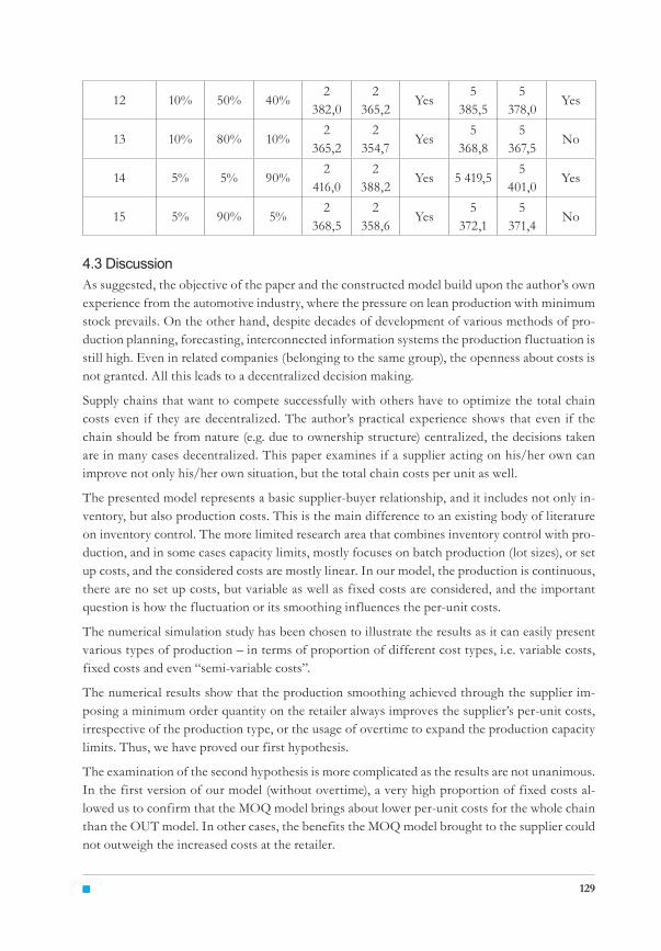
This time, we explore the effects of production smoothing (MOQ vs OUT model) on the exam-ple of 15 different scenarios to illustrate various types of production, i.e. with various propor-tions of material costs, fixed costs and personnel costs. The list is not as comprehensive as in the previous chapter, but the selected 15 scenarios should cover and illustrate a whole range of pos-sible cost type proportions as each of the cost type would be represented in its low and also high proportion with various combinations of the other two cost types. The scenarios considered are shown in the first columns of Tab. �.

Again the usage of MOQ to limit the retailer’s replenishment orders causes stabilizing of pro-duction level. The bullwhip ratio (equation 1�) for OUT model is 0,58� whereas for the MOQ model 0,1��. As a result, the supplier’s per-unit costs are always lower in the MOQ model than in the OUT model (see Tab. �).

The question of total chain costs per unit gets more complex. The number of influences is get-ting higher and the evaluation of their effect more intricate. We can state that when the propor-

2 100

2 150

2 200

2 250

2 300

2 350

2 400

500 505 510 515 520 525 530 535 540 545 550

MC 10 - FC 10 - PC 80 MC 10 - FC 80 - PC 10


tion of material costs (a truly variable cost type) is high, there is not much point in smoothing the production, it may even have negative effects on the chain costs. However, as the proportion of fixed and especially the proportion of the personnel costs are getting higher, the more positive effect on total chain per-unit costs stabilizing the production level has. In Tab. �, we can see the results of all 15 scenarios.

We can sum up that in the defined environment, a supplier imposing a minimum order quantity on a retailer’s orders leads in all of the scenarios to more stable production levels, and improve-ment in supplier’s per-unit costs. However, the influence on the total supply chain per-unit cost is ambivalent, in some scenarios, the production smoothing leads to statistically significant im-provement of total chain per-unit costs, in others, it even has a negative effect on these costs.

Tab. � – Supplier’s and total costs per unit (with overtime). Source: own

Scen

ario

Mat

eria

l Cos

ts

Fixe

d C

osts

Pers

onne

l Cos

ts

Supp

lier’s

cos

ts p

er

unit

OU

T

Supp

lier’s

cos

ts p

er

unit

MO

Q

Stat

istic

ally

sign

ifi-

cant

impr

ovem

ent

Tota

l cha

in c

osts

per

un

it O

UT

Tota

l cha

in c

osts

per

un

it M

OQ

Stat

istic

ally

sign

ifi-

cant

impr

ovem

ent

1 90% 5% 5%�

�65,0�

�6�,0Yes

5 �68,5

5 ��5,8

No

� 80% 10% 10%�

��9,9�

��6,0Yes

5 �8�,5

5 �88,8

No

� 60% �0% 10%�

�04,��

�98,5Yes

5 �0��,9

5 �11,� No

4 45% 10% 45%�

�4�,1�

��,5Yes

5 �45,��

5 �40,4

Yes

5 40% 50% 10%�

��8,��

��1,0Yes

5 ��,�

5 ��,8

No

6 �5% �0% �5%�

�48,��

��5,�Yes

5 �5�,�

5 �48,1

Yes

�� ,�% ��,�% ��,�%�

�49,8�

��6,6Yes

5 �5�,4

5 �49,4

Yes

8 �5% 50% �5%�

�55,��

�4�,1Yes

5 �58,9

5 �55,9

Yes

9 15% ��0% 15%�

�61,9�

�50,8Yes

5 �65,5

5 �6�,��

No

10 10% 10% 80%�

404,�� 9,1 Yes

5 40��,9

5 �91,9

Yes

11 10% �0% 60%�

�9�,1�

��,1Yes

5 �96,��

5 �85,0

Yes

129

1� 10% 50% 40%�

�8�,0�

�65,�Yes

5 �85,5

5 ��8,0

Yes

1� 10% 80% 10%�

�65,��

�54,��Yes

5 �68,8

5 �6��,5

No

14 5% 5% 90%�

416,0�

�88,�Yes 5 419,5

5 401,0

Yes

15 5% 90% 5%�

�68,5�

�58,6Yes

5 ��,1

5 ��1,4

No

4.3 DiscussionAs suggested, the objective of the paper and the constructed model build upon the author’s own experience from the automotive industry, where the pressure on lean production with minimum stock prevails. On the other hand, despite decades of development of various methods of pro-duction planning, forecasting, interconnected information systems the production fluctuation is still high. Even in related companies (belonging to the same group), the openness about costs is not granted. All this leads to a decentralized decision making.

Supply chains that want to compete successfully with others have to optimize the total chain costs even if they are decentralized. The author’s practical experience shows that even if the chain should be from nature (e.g. due to ownership structure) centralized, the decisions taken are in many cases decentralized. This paper examines if a supplier acting on his/her own can improve not only his/her own situation, but the total chain costs per unit as well.

The presented model represents a basic supplier-buyer relationship, and it includes not only in-ventory, but also production costs. This is the main difference to an existing body of literature on inventory control. The more limited research area that combines inventory control with pro-duction, and in some cases capacity limits, mostly focuses on batch production (lot sizes), or set up costs, and the considered costs are mostly linear. In our model, the production is continuous, there are no set up costs, but variable as well as fixed costs are considered, and the important question is how the fluctuation or its smoothing influences the per-unit costs.

The numerical simulation study has been chosen to illustrate the results as it can easily present various types of production – in terms of proportion of different cost types, i.e. variable costs, fixed costs and even “semi-variable costs”.

The numerical results show that the production smoothing achieved through the supplier im-posing a minimum order quantity on the retailer always improves the supplier’s per-unit costs, irrespective of the production type, or the usage of overtime to expand the production capacity limits. Thus, we have proved our first hypothesis.

The examination of the second hypothesis is more complicated as the results are not unanimous. In the first version of our model (without overtime), a very high proportion of fixed costs al-lowed us to confirm that the MOQ model brings about lower per-unit costs for the whole chain than the OUT model. In other cases, the benefits the MOQ model brought to the supplier could not outweigh the increased costs at the retailer.


In the second model (with overtime), the results are even more ambivalent. In case the truly vari-able costs proportion is high, we cannot confirm the hypothesis, as the production smoothing brings higher per-unit costs for the whole chain. The higher the proportion of the fixed costs and especially the personnel costs (“semi-variable”) the more positive effect on the whole chain per-unit costs. In a number of presented scenarios, we can confirm the second hypothesis and state that the production smoothing (MOQ model) brings about lower whole chain per-unit costs than in the OUT model. Thus we extend the findings of Chan and Muckstadt (1999) and state that while considering variable, fixed and “semi-variable” production costs, the produc-tion smoothing through a modified-modified base-stock policy might not always bring about improvement of the whole chain per-unit costs. It depends on the cost type proportions.

In this paper, we examine the total chain per-unit costs and in some cases with production smoothing (MOQ model), they are decreasing. However, the advantages are on the side of the supplier and the retailer finds himself in a worse situation than before. For the chain to improve its competitiveness, the supplier’s advantage would have to be shared also with the retailer, and to such an extent that brings also the retailer to a more advantageous position than in the OUT model. Only then, the retailer can share part of the benefit with the final customer, in other words, make the chain more competitive. The mechanisms of this benefit sharing between a supplier and a retailer reaches beyond the scope of this paper and we refer the reader to, e.g., Govindan and Popiuc (�011) who discuss the coordination in supply chains via contracts.

5. CONCLUsIONIn this paper, we explore and evaluate the effects of production smoothing on total chain costs in a decentralized capacitated production-inventory system consisting of one retailer holding stock of a finished product and one supplier producing to retailer’s order and holding no inven-tory. The novel contribution of this paper is considering a continuous (no set-ups considered) production running close to its full capacity. The capacity utilization plays an important role. Therefore, material, personnel as well as fixed costs of the supplier’s production are considered when evaluating the effects of production smoothing.

The retailer orders in an order-up-to predefined level manner (OUT) and is constrained by the production capacity level mutually agreed in advance. The production smoothing in the second model is achieved “unilaterally” by the supplier by imposing a minimum order quantity (MOQ) on the retailer, thus constricting the retailer’s replenishment orders between an upper (capacity) and lower (MOQ) bound.

The effects of the production smoothing is observed in two settings, one without any use of overtime, the second with a use of overtime to expand the limited production capacity, and in multiple scenarios with various combinations of production cost type proportions.

In both settings, the production smoothing brings about improvement of supplier’s per-unit costs, while the effects on the total chain per-unit costs is ambivalent. In the model setting without using the overtime, the higher the proportion of fixed and personnel costs is, the more positive effects of production smoothing on total chain per-unit costs are. In the model with us-ing the overtime, the higher the proportion of fixed and especially personnel costs is, the more positive effect on total chain per-unit costs is.

131

ReferencesAffisco, J. F., Paknejad, M. J., & Nasri, F. (�00�). Quality improvement and setup reduction in the joint economic lot size model. European Journal of Operational Research, 14�(�), 49��-508. http://dx.doi.org/10.1016/S0��-��1��(01)00�08-�

Arrow, K. J., Harris, T., & Marschak, J. (1951). Optimal inventory policy. Econometrica: Journal of the Econometric Society, �50-��. http://dx.doi.org/10.��0��/190681�

Aviv, Y., & Federgruen, A. (199��). Stochastic inventory models with limited production capacity and periodically varying parameters. Probability in the Engineering and Informational Sciences, 11, 10��-1�5. http://dx.doi.org/10.101��/S0�69964800004��1X

Banerjee, A. (1986). A joint economic-lot-size model for purchaser and vendor. Decision Sciences, 1�� (�), �9�-�11. ISSN 0011-��15. http://dx.doi.org/10.1111/j.1540-5915.1986.tb00��8.x

Banerjee, A., & Burton, J. S. (1994). Coordinated vs. independent inventory replenishment policies for a vendor and multiple buyers. International Journal of Production Economics, �5 (1-�), �15-��. http://dx.doi.org/10.1016/09�5-5��(94)90084-1

Ben-Daya, M., & Hariga, M. (�004). Integrated single vendor single buyer model with stochastic demand and variable lead time. International Journal of Production Economics, 9�(1), ��5-80. http://dx.doi.org/10.1016/j.ijpe.�00�.09.01�

Ben-Daya, M., Darwish, M., & Ertogral, K. (�008). The joint economic lot sizing problem: Review and extensions. European Journal of Operational Research, 185(�), ��6-��4�. http://dx.doi.org/10.1016/j.ejor.�006.1�.0�6

Cachon, G. (1999). Competitive and cooperative inventory management in a two-echelon supply chain with lost sales. Fuqua School of Business, Duke University, Durham, NC. Working paper.

Chan, E. W., & Muckstadt, J. A. (1999). The Effects of load smoothing on inventory levels in a capacitated production and inventory system. School of Operations Research and Industrial Engineering (No. 1�51). Technical Report.

Chang, C. T., Teng, J. T., & Goyal, S. K. (�008). Inventory lot-size models under trade credits: a review. Asia-Pacific Journal of Operational Research, �5(01), 89-11�. http://dx.doi.org/10.114�/S0�1��595908001651

Chang, H. C., Ouyang, L. Y., Wu, K. S., & Ho, C. H. (�006). Integrated vendor–buyer cooperative inventory models with controllable lead time and ordering cost reduction. European Journal of Operational Research, 1��0(�), 481-495.

Chang, J. H., & Chiu, H. N. (�005). A comprehensive review of lot streaming. International Journal of Production Research, 4�(8), 1515-15�6. http://dx.doi.org/10.1080/00�0��54041��1��5�96

Chen, F., & Zheng, Y. S. (1994). Lower bounds for multi-echelon stochastic inventory systems. Management Science, 40(11), 14�6-144�. http://dx.doi.org/10.1�8��/mnsc.40.11.14�6

Clark, A. J., & Scarf, H. (1960). Optimal policies for a multi-echelon inventory problem. Management science, 6(4), 4��5-490.

1.

�.

�.

4.

5.

6.

��.

8.

9.

10.

11.

1�.

1�.

14.


Disney, S. M., Farasyn, I., Lambrecht, M., Towill, D., & Van de Velde, W. (�006). Dampening variability by using smoothing replenishment rules. Available at SSRN 8��588. http://dx.doi.org/10.�1�9/ssrn.8��588

Ertogral, K., Darwish, M., & Ben-Daya, M. (�00��). Production and shipment lot sizing in a vendor–buyer supply chain with transportation cost. European Journal of Operational Research, 1��6(�), 159�-1606.

Federgruen, A., & Zipkin, P. (1984). Computational issues in an infinite horizon multiechelon inventory model. Operations Research. ��(4) 818–8�6. http://dx.doi.org/10.1�8��/opre.��.4.818

Federgruen, A., & Zipkin, P. (1986a). An inventory model with limited production capacity and uncertain demands I. The average-cost criterion. Mathematics of Operations Research, 11(�), 19�-�0��. http://dx.doi.org/10.1�8��/moor.11.�.19�

Federgruen, A., & Zipkin, P. (1986b). An inventory model with limited production capacity and uncertain demands II. The discounted-cost criterion. Mathematics of Operations Research, 11(�), �08-�15. http://dx.doi.org/10.1�8��/moor.11.�.�08

Glasserman, P., & Tayur, S. (1994). The stability of a capacitated, multi-echelon production-inventory system under a base-stock policy. Operations Research. 4�(5) 91�–9�5. http://dx.doi.org/10.1�8��/opre.4�.5.91�

Glasserman, P., & Tayur, S. (1995). Sensitivity analysis for base-stock levels in multiechelon production-inventory systems. Management Science. 41(�) �6�–�81. http://dx.doi.org/10.1�8��/mnsc.41.�.�6�

Glock, C. H. (�011). A multiple-vendor single-buyer integrated inventory model with a variable number of vendors. Computer & Industrial Engineering, 60 (1), 1��-18�. http://dx.doi.org/10.1016/j.cie.�010.11.001

Glock, C. H. (�01�). The joint economic lot size problem: A review. International Journal of Production Economics, 1�5, 6��1-686. ISSN 09�5-5��. http://dx.doi.org/10.1016/j.ijpe.�011.10.0�6

Govindan, K., & Popiuc, M. N. (�011). Overview and classification of coordination contracts within forward and reverse supply chains. Discussion Papers on Business and Economics, ��, 5-��.

Goyal, S. K. (19��). An integrated inventory model for a single supplier-single customer problem. The International Journal of Production Research, 15 (1), 10��-111. ISSN 1�66-588X. http://dx.doi.org/10.1080/00�0��54��0894�10��

Harris, F. W. (191�). How many parts to make at once. Factory, The Magazine of Management, 191�, vol 10, iss. �, pp. 1�5-1�6.

Hoque, M. A., & Goyal, S. K. (�006). A heuristic solution procedure for an integrated inventory system under controllable lead-time with equal or unequal sized batch shipments between a vendor and a buyer. International Journal of Production Economics, 10�(�), �1��-��5. http://dx.doi.org/10.1016/j.ijpe.�005.0�.01�

Johnson, L. A., & Montgomery, D. C. (19��4). Operations research in production planning, scheduling, and inventory control (Vol. 6). New York: Wiley.

15.

16.

1��.

18.

19.

�0.

�1.

��.

��.

�4.

�5.

�6.

��.

�8.

133

Kapuscinski, R., & Tayur, S. (1998). A capacitated production-inventory model with periodic demand. Operations Research, 46(6), 899-911.

Karlin, S., & Scarf, H. (1958). Inventory models of the Arrow-Harris-Marschak type with time lag. Studies in the mathematical theory of inventory and production, 1, 155.

Kijima, M., & Takimoto, T. (1999). A (T, S) inventory/production system with limited production capacity and uncertain demands. Operations research letters, �5(�), 6��-��9. http://dx.doi.org/10.1016/S016��-6��(99)000��-4

Levi, R., Roundy, R. O., Shmoys, D. B., & Truong, V. A. (�008). Approximation algorithms for capacitated stochastic inventory control models. Operations Research, 56(5), 1184-1199. http://dx.doi.org/10.1�8��/opre.1080.0580

Modigliani, F., & Hohn, F. E. (1955). Production planning over time and the nature of the expectation and planning horizon. Econometrica, Journal of the Econometric Society, 46-66. http://dx.doi.org/10.��0��/1905580

Pentico, D. W., & Drake, M. J. (�011). A survey of deterministic models for the EOQ and EPQ with partial backordering. European Journal of Operational Research, �14(�), 1��9-198. http://dx.doi.org/10.1016/j.ejor.�011.01.048

Pujawan, I. N., & Kingsman, B. G. (�00�). Joint optimisation and timing synchronisation in a buyer supplier inventory system. International Journal of Operations and Quantitative Management, 8(�), 9�-110.

Sari, D. P., Rusdiansyah, A., & Huang, L. (�01�). Models of joint economic lot-sizing problem with time-based temporary price discounts. International Journal of Production Economics, 1�9(1), 145-154. http://dx.doi.org/10.1016/j.ijpe.�011.1�.014

Spengler, J. (1950). Vertical integration and antitrust policy. Journal of Political Economy, 58, �4��–�5�. http://dx.doi.org/10.1086/�56964

Tayur, S. R. (199�). Computing the Optimal Policy for Capacitated Inventory Models. Communication in Statistics, Stochastic Models, 9(4), 585-598. http://dx.doi.org/10.1080/15��6�49�0880��8�

Wagner, H. M., & Whitin, T. M. (1958). Dynamic version of the economic lot size model. Management science, 5(1), 89-96. http://dx.doi.org/10.1�8��/mnsc.5.1.89

Wilson, R. H. (19�4). A scientific routine for stock control. Harvard business review, 1�(1), 116-1�8.

Contact informationIng. Lucie Synáková, MBATechnical University of Liberec, Faculty of EconomicsStudentská 1402/2, 46117 Liberec, Czech RepublicEmail: [email protected]

�9.

�0.

�1.

��.

��.

�4.

�5.

�6.

��.

�8.

�9.

40.

production smoothing and cost performance in a … · 117 production smoothing and cost performance...

Documents