production-process modelling based on production ...msc.fe.uni-lj.si/papers/ijcim_gradisar.pdf ·...

Production-process modelling based on production-managementdata: a Petri-net approach

D. GRADISAR*{{ and G. MUSIC{

{Faculty of Electrical Engineering, University of Ljubljana, Trzaska 25, 1000 Ljubljana, Slovenia{Jozef Stefan Institute, Jamova 39, 1000 Ljubljana, Slovenia

During the development of a production control system, an appropriate model of the

production process is needed to evaluate the various control strategies. This paper

describes how to apply timed Petri nets and existing production data to the modelling of

production systems. Information concerning the structure of a production facility and the

products that can be produced is usually given in production-data management systems.

We describe a method for using these data to construct a Petri-net model algorithmically.

The timed Petri-net simulator, which was constructed in Matlab, is also described. This

simulator makes it possible to introduce heuristics, and, in this way, various production

scenarios can be evaluated. To demonstrate the applicability of our approach, we applied

it to a scheduling problem in the production of furniture fittings.

Keywords: Timed Petri nets; Modelling; Scheduling; Production systems; Simulation

1. Introduction

As the role played by information systems in production

control increases, the need for a proper evaluation of the

various decisions in both the design and operational stages

of such systems is becoming more and more important.

In general, an appropriate model of a production process

is needed in order to cope with its behaviour. However, this

behaviour is often extremely complex. When the behaviour

is described by a mathematical model, formal methods can

be used, which usually improve the understanding of

systems, allow their analysis and help in implementation.

Within the changing production environment the effective-

ness of production modelling is, therefore, a prerequisite

for the effective design and operation of manufacturing

systems.

Scheduling is a fundamental problem in the control of

any resource-sharing organization. Scheduling problems

are very complex and many have been proven to be NP

hard (Jain and Meeran 1999). There are several major

approaches to scheduling. Formal, theoretically oriented

approaches have to ignore many practical constraints in

order to solve these problems efficiently (Richard and

Proust 1998). This is the reason why only a few real

applications exist in the industrial environment (Hauptman

and Jovan 2004). Mathematical programming approaches

are computationally demanding and often cannot achieve

feasible solutions to practical problems (Jain and Meeran

1999). Soft-computing approaches, e.g. genetic algorithms

and neural networks, require considerable computation

and only yield sub-optimal solutions. Instead, heuristic

dispatching rules (Panwalker and Iskaneder 1977,

Blackstone et al. 1982), such as Shortest Processing Time

(SPT) or Longest Processing Time (LPT), are commonly

used in practice. An interesting property of heuristic

dispatching rules is that they can easily be used in

conjunction with production models derived within differ-

ent mathematical modelling frameworks, e.g. the disjunc-

tive graph model (Bła_zewicz et al. 1996, 2000), timed

automata (Abdeddaim et al. 2006), and Petri nets (Murata

1989, Zhou and Venkatesh 1999).

Petri nets (PN) represent a powerful graphical and

mathematical modelling tool. The different abstraction

levels of Petri-net models and their different interpretations

make them especially usable for life-cycle design (Silva and

Teruel 1997). Many different extensions of classical Petri

*Corresponding author. Email: [email protected]

International Journal of Computer Integrated Manufacturing, Vol. 00, No. 0, Month 2007, 1 – 17

International Journal of Computer Integrated ManufacturingISSN 0951-192X print/ISSN 1362-3052 online ª 2007 Taylor & Francis

http://www.tandf.co.uk/journalsDOI: 10.1080/09511920601103064

nets exist, and these are able to model a variety of real

systems. In particular, timed Petri nets can be used to

model and analyse a wide range of concurrent discrete-

event systems (Zuberek 1991, Van der Aalst 1996, Zuberek

and Kubiak 1999, Bowden 2000). Several previous studies

have addressed the timed-Petri-net-based analysis of

discrete-event systems. Lopez-Mellado (2002), for example,

deals with the simulation of the deterministic timed Petri

net for both timed places and timed transitions by using the

firing-duration concept of time implementation. Van der

Aalst (1998) discusses the use of Petri nets in the context of

workflow management. Gu and Bahri (2002) discuss the

usage of Petri nets in the design and operation of a batch

process. There is a lot of literature on the applicability of

PNs in the modelling, analysis, synthesis and implementa-

tion of systems in the manufacturing-applications domain.

A survey of the research area and a comprehensive biblio-

graphy can be found in Zhou and Venkatesh (1999).

Recalde et al. (2004) give an example-driven tour of Petri

nets and manufacturing systems where the use of Petri-net

production models through several phases of the design

life-cycle is presented.

A straightforward way of using the heuristic rules within

a Petri-net modelling framework is to incorporate the rules

for the conflict-resolution mechanism in an appropriate

Petri-net simulator. Many different Petri-net simulators

exist, some of which also support timed Petri nets, and they

usually support random decisions to make a choice in the

case of conflicts. The Petri-net toolbox for Matlab

(Matcovschi et al. 2003) allows the use of priorities or

probabilities to make a choice about a conflicting transition

to fire. CPN Tools can also be used for the modelling,

simulating and analyses of untimed and timed Petri nets

(Ratzer et al. 2003).

One of the central issues when using Petri nets in

manufacturing is the systematic synthesis of Petri-net

models for automated manufacturing systems. Problems

arise when the complexity of a real-world system leads to a

large Petri net having many places and transitions (Zhou

et al. 1992). A common approach is to model the com-

ponents and build the overall systems in a bottom-up

manner. However, a Petri net constructed by merging

arbitrary sub-nets is difficult to analyse, and, furthermore,

an early design error can lead to an incorrect model. Zhou

et al. (1992) propose a hybrid methodology that builds a

model by combining the top-down refinement of operations

and the bottom-up assignment of resources. Another

approach is the use of well-defined net modules and

restricting their interaction. By merging corresponding

sub-nets in a predefined way a set of desired properties of

the resulting net is maintained (Jeng 1997). But the

synthesis of complex models remains tedious and error-

prone. Therefore, a number of researchers have put toward

the idea of modelling a flexible manufacturing system

(FMS) with a FMS modelling language. The language

model is then automatically translated into one of the

standard PN classes, such as Coloured Petri nets – CPN

(Arjona-Suarez and Lopez-Mellado 1996) or Generalized

stochastic Petri nets – GSPN (Xue et al. 1998). Some

researchers have also proposed the translation into special

PN classes, e.g. B-nets (Yu et al. 2003a). Other approaches

to the automatic synthesis of PN models are presented by

Camurri et al. (1993), Ezpeleta and Colom (1997) and

Basile et al. (2006) and special PN classes appropriate for

modelling FMS appear in Proth et al. (1997), Van der Aalst

(1998) and Janneck and Esser (2002).

On the other hand, Huang et al. (1995) use a discrete-

event matrix model of a FMS, which can be built based on

standard manufacturing data, and can also be interpreted

as a Petri net. This latter approach is particularly attractive

when there are data concerning the production process

available within some kind of production-management

information system. Using these data, a model-building

algorithm can be embedded within the information system.

In this paper we propose a method for using the data from

management systems, such as Manufacturing Resource

Planning (MRP II) systems (Wortmann 1995), to automate

the procedure of building up the Petri-net model of a

production system. Instead of using a discrete-event matrix

model, the Petri net is built directly in a top-down manner,

starting from the bill of materials (BOM) and the routings

(Wortmann 1995). The BOM and the routing data,

together with the available resources, form the basic

elements of the manufacturing process. These data can be

effectively used to build up a detailed model of the

production system with Petri nets. The product structure

given in the form of the BOM and the process structure in

the form of routings have also been used by other

researchers. Czerwinski and Luh (1994) propose a method

for scheduling products that are related through the BOM

using an improved Lagrangian Relaxation technique. An

approach presented by Yeh (1997) maintains production

data by using a bill of manufacture (BOMfr), which

integrates the BOM and the routing data. Production data

are then used to determine the production jobs that need to

be completed in order to meet demands. Compared to

previous work, the method proposed in this paper builds a

Petri-net model that can be further analysed, simulated and

used for scheduling purposes.

First we define timed Petri nets, where time is introduced

by using the holding-durations concept. A general class of

place/transition (P/T) nets supplemented by timed transi-

tions is used. Although several special classes of PNs have

been defined, there was no need to either restrict the

behaviour of the P/T nets or extend their modelling power

during the work presented in this paper. The use of some

kind of high-level Petri nets would, however, probably be

needed in a real industrial implementation. Practical

2 D. Gradisar and G. Musi�c

experience also shows that, for most applications in a real

manufacturing environment, the use of deterministic time

delays is sufficient. Adopting the class of timed P/T nets, a

method for modelling the basic production activities with

such a Petri net is described. A corresponding algorithm of

automatic model building is presented. For a defined, timed

Petri net a simulator was built, for which different heuristic

rules can be introduced for scheduling purposes. The

applicability of the proposed approach was illustrated

using a practical scheduling problem, where data con-

cerning the production facility is given with the BOM and

the routings. The model constructed using the proposed

method was used to determine a schedule for the pro-

duction operations.

In the next section we describe timed Petri nets that can be

used for the modelling and analysis of a production system.

In section 3 the method for modelling the production system

using data from the production-management system is

presented. Section 4 explains the simulator/scheduler that

was built for the purposes of scheduling; it can use different

heuristic dispatching rules. An illustrative application of

modelling an assembly process and developing a schedule

using timed Petri nets is given in section 5. Finally, the

conclusions are presented in section 6.

2. Timed Petri nets

Petri nets are a graphical and mathematical modelling tool

that can be used to study systems that are characterized as

being concurrent and asynchronous.

The basic Place/Transition Petri net (Zhou and

Venkatesh 1999) is represented by the multiple

PN ¼ ðP;T; I;O;M0Þ;

where P¼ {p1, p2, . . . , pg} is a finite set of places; T¼ t1,

t2, . . . , th is a finite set of transitions; I : ðP� TÞ ! IN is the

input arc function. If there exists an arc with weight k

connecting pi to tj, then I(pi, tj)¼ k, otherwise I(pi, tj)¼ 0;

O : ðP� TÞ ! IN is the output arc function. If there exists

an arc with weight k connecting tj to pi, then O(pi, tj)¼ k,

otherwise O(pi, tj)¼ 0; M : P ! IN is the marking; and M0

is the initial marking.

Functions I and O define the weights of the directed arcs,

which are represented by numbers placed along the arcs. In

the case when the weight is 1, this marking is omitted, and in

the case when the weight is 0, the arc is omitted. Let .tj�P

denote the set of places which are inputs to transition tj2T,

i.e. there exists an arc from every pi2 .tj to tj. A transition tjis enabled by a given marking if, and only if, M(pi)� I

(pi, tj),8pi2 .tj. An enabled transition can fire, and as a

result remove tokens from input places and create tokens in

output places. If the transition tj fires, then the new marking

is given by M0(pi)¼M(pi)þO(pi, tj)7 I(pi, tj), 8pi2P.

The structure of the Petri net can also be given in a

matrix representation (Zhou and Venkatesh 1999). We

define a g6h input matrix I, whose (i, j) entry is I(pi, tj).

Similarly, we define an output matrix O of the same

size, whose elements are defined by O(pi, tj). Matrices I

and O precisely describe the structure of the Petri net

and make it possible to explore the structure using linear

algebraic techniques. Furthermore, the marking vector M

where Mi¼M(pi), and a firing vector u with a single non-

zero entry uj¼ 1, which indicates a transition tj that fires,

are defined. Using these matrices we can now write a

state equation Mkþ1¼Mkþ (O7 I) � uk. The subscript k

denotes the kth firing in some firing sequence.

An important concept in PNs is that of conflict. Two

events are in conflict if either one of them can occur, but

not both of them. Conflict occurs between transitions

that are enabled by the same marking, where the firing of

one transition disables the other transition. Also, parallel

activities or concurrency can easily be expressed in terms

of a PN. Two events are parallel if both events can

occur in any order without conflicts. A situation

where conflict and concurrency are mixed is called a

confusion.

The concept of time is not explicitly given in the original

definition of Petri nets. However, for the performance

evaluation and scheduling problems of dynamic systems it

is necessary to introduce time delays. Given that a

transition represents an event, it is natural that time delays

should be associated with transitions. Time delays may be

either deterministic or stochastic. In this work, timed Petri

nets with deterministic time delays are used to model the

behaviour of a production system.

As described by Bowden (2000) there are three basic

ways of representing time in Petri nets: firing durations,

holding durations and enabling durations. The firing-

duration principle says that when a transition becomes

enabled it removes the tokens from input places immedi-

ately but does not create output tokens until the firing

duration has elapsed. Zuberek (1991) gives a well-defined

description of this principle. When using the holding-

duration principle, a created token is considered unavail-

able for the time assigned to the transition that created the

token. The unavailable token cannot enable a transition

and therefore causes a delay in the subsequent transition

firings. This principle is graphically represented in figure 1,

where the available tokens are schematized with the

corresponding number of undistinguishable (black) tokens

and the unavailable tokens are indicated by the center not

being filled. The time duration of each transition is given

beside the transition, e.g. f(t1)¼ td. When the time duration

is 0 this denotation is omitted. In figure 1, t denotes a model

time represented by a global clock and tf denotes the firing

time of a transition. With enabling durations the firing of

the transitions happens immediately and the time delays are

Production-process modelling based on production-management data 3

represented by forcing transitions that are enabled to stay

so for a specified period of time before they can fire.

Holding durations and firing durations are in fact the

same way of representing time. We prefer the use of holding

durations, because in comparison with firing durations they

do not have transitions that remain active over periods of

time. Thus, the schematics of holding durations are closer

to those of non-timed Petri nets. The main difference

between using holding and enabling durations can be seen

in a Petri net where confusion appears. In this case, more

transitions are enabled by one marking. When the enabling

duration policy is used, the firing of one transition can

interrupt the enabling of other transitions, as the marking,

which has enabled the previous situation, has changed

(Bowden 2000). It is reasonable to use holding durations

when modelling production processes where the operations

are non pre-emptive.

By using holding durations the formal representation of

the timed Petri net is extended with the information of time,

represented by the multiple

TPN ¼ ðP;T; I;O; s0; fÞ;

where P, T, I, O are the same as above, s0 is the initial state

of the timed Petri net, and f : T ! IRþ0 is the function that

assigns a non-negative deterministic time-delay to every

tj2T. The delays can be represented by 16h row vector f

whose jth entry is f(tj).

The state of a timed Petri net is a combination of three

functions

s ¼ ðm; n; rÞ;

where m :P ! IN is a marking function of available tokens.

It defines a g61 column vector m whose ith entry is m(pi);

n :P ! IN is a marking function of unavailable tokens. It

defines a g61 column vector n whose ith entry is n(pi); and

r is the remaining-holding-time function that assigns values

to a number of local clocks that measure the remaining

time for each unavailable token (if any) in a place.

Assuming l unavailable tokens in pi, i.e. n(pi)¼ l, the

remaining-holding-time function r(pi) defines a vector of

l positive real numbers denoted by r(pi)¼ [r(pi)[1],

r(pi)[2], . . . , r(pi)[l]]; r is empty for every pi, where n(pi)¼ 0.

A transition tj is enabled by a given marking if, and only

if, m(pi)� I(pi, tj),8 pi2 .tj. The firing of transitions is

considered to be instantaneous. A new local clock is created

for every newly created token and the initial value of the

clock is determined by the delay of the transition that

created the token. When no transition is enabled, the time

of the global clock is incremented by the value of the

smallest local clock. An unavailable token in a place where

a local clock reaches zero becomes available and the clock

is destroyed. The enabling condition is checked again. The

procedure for determining a new state is described in detail

in section 4.

3. The modelling of production systems

This section deals with models for production facilities.

These models play a role in the design and the operational

control of a plant. Petri nets are a family of tools that

provide a framework or working paradigm which can be

used for many of the problems that appear during the life-

cycle of a production system (Silva and Teruel 1997). If

used in all stages, an additional benefit of improving the

communication between these stages is achieved.

We present a method for modelling production systems

using timed Petri nets based on data from production-

management systems for the purpose of performance

control. Van der Aalst (1996) provides a method for

mapping scheduling problems onto timed Petri nets, where

the standard Petri-net theory can be used. To support the

modelling of scheduling problems, he proposed a method

to map tasks, resources and constraints onto a timed Petri

net. In this paper a different representation of time in Petri

nets is used, and the structure of the model is derived from

existing production-management data (Wortmann 1995). A

method for recognizing basic production elements from the

management system’s database is provided.

When timed Petri nets are used, it is possible to derive

performance measures such as makespan, throughput, pro-

duction rates, and other temporal quantities. In this work

the simulation of a timed Petri net is used to estimate the

performance measures and evaluate different priority rules.

3.1. The class of production system

With the method presented here, several scheduling pro-

blems that appear in production systems can be solved. The

production systems are considered where management

systems (MRP II) are used to plan the production process.

Figure 1. Timed Petri net with holding durations.


The system generates work orders that interfere with the

demands for the desired products. Different jobs are needed

to produce a desired product. In general, more operations

have to be performed using different resources in order to

complete a specific job. To complete a specific product,

more sub-products may be needed. The BOM defines a list

of components. These components determine sub-jobs that

are needed to manufacture a parent item. In this way the

general scheduling problem is defined and can be given as:

. n jobs are to be processed: J¼ {Jj}, j¼ 1, . . . , n;

. m resources are available: M¼ {Mi}, i¼ 1, . . . , m;

. each job Ji is composed of nj operations: Oj¼ {ojk},

k¼ 1, . . . , nj;

. each operation can be processed on (more) different

sets of resources Sjkl2R; l determines the number of

different sets;

. the processing time of each operation ojkl, using

resource set Sjkl, is defined as Tjkl;

. precedence constraints are used to define that one job

has to be performed before another.

Using this definition, the following assumptions have to be

considered.

. Resources are always available and never break

down.

. Each resource can process a limited number of

operations. This limitation is defined by the capacity

of resources.

. Operations are non pre-emptive.

. When an operation is performed, it is desirable to

free the resources so that they can become available

as soon as possible. Intermediate buffers between

processes are common solutions.

. Processing times are deterministic and known in

advance.

. Work orders define the quantity of desired products

and the starting times. Orders that are synchronized

in time are considered jointly.

. In the case where a job requires sub-products, for

each of the additions, sub-jobs are to be defined.

3.2. The modelling of production activities

First, a method of describing the production-system

activities with timed Petri nets using the holding-duration

representation of time is presented. The places represent

resources and jobs/operations, and the transitions represent

decisions or rules for resource assignment/release and for

starting/ending jobs.

To make a product, a set of operations has to be per-

formed. We can think of an operation as a set of events and

activities. Using a timed PN, events are represented by

transitions and activity is associated with the presence of a

token in a place.

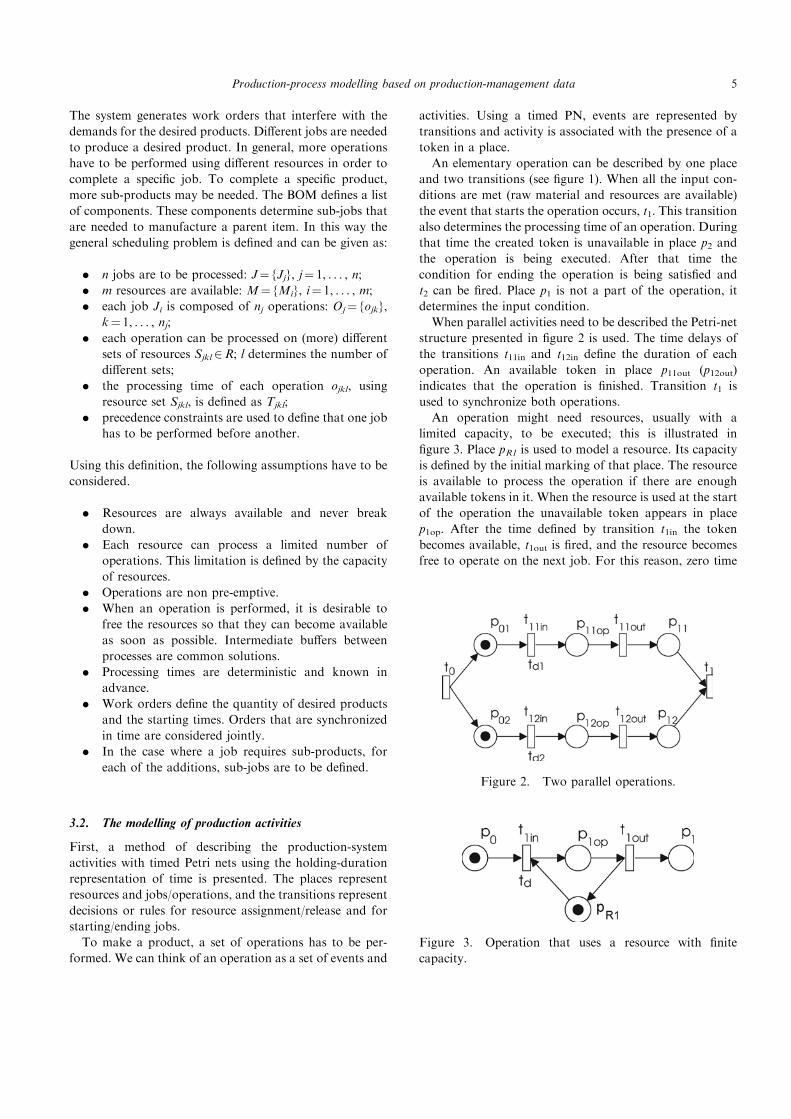
An elementary operation can be described by one place

and two transitions (see figure 1). When all the input con-

ditions are met (raw material and resources are available)

the event that starts the operation occurs, t1. This transition

also determines the processing time of an operation. During

that time the created token is unavailable in place p2 and

the operation is being executed. After that time the

condition for ending the operation is being satisfied and

t2 can be fired. Place p1 is not a part of the operation, it

determines the input condition.

When parallel activities need to be described the Petri-net

structure presented in figure 2 is used. The time delays of

the transitions t11in and t12in define the duration of each

operation. An available token in place p11out (p12out)

indicates that the operation is finished. Transition t1 is

used to synchronize both operations.

An operation might need resources, usually with a

limited capacity, to be executed; this is illustrated in

figure 3. Place pR1 is used to model a resource. Its capacity

is defined by the initial marking of that place. The resource

is available to process the operation if there are enough

available tokens in it. When the resource is used at the start

of the operation the unavailable token appears in place

p1op. After the time defined by transition t1in the token

becomes available, t1out is fired, and the resource becomes

free to operate on the next job. For this reason, zero time

Figure 2. Two parallel operations.

Figure 3. Operation that uses a resource with finite

capacity.


needs to be assigned to the transition t1out. An additional

place p1 models the control flow. When the token is present

in this place, the next operation can begin.

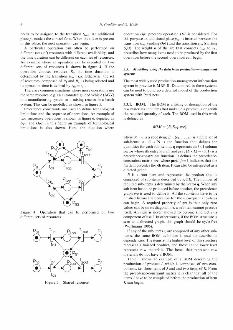
A particular operation can often be performed on

different (sets of) resources with different availability, and

the time duration can be different on each set of resources.

An example where an operation can be executed on two

different sets of resources is shown in figure 4. If the

operation chooses resource R3, its time duration is

determined by the transition t2in¼ td2. Otherwise, the set

of resources, composed of R1 and R2, is being selected and

its operation time is defined by t1in¼ td1.

There are common situations where more operations use

the same resource, e.g. an automated guided vehicle (AGV)

in a manufacturing system or a mixing reactor in a batch

system. This can be modelled as shown in figure 5.

Precedence constraints are used to define technological

limitations and the sequence of operations. An example of

two successive operations is shown in figure 6, depicted as

Op1 and Op2. In this figure an example of technological

limitations is also shown. Here, the situation where

operation Op1 precedes operation Op3 is considered. For

this purpose an additional place ppr1 is inserted between the

transition t1out (ending Op1) and the transition t3in (starting

Op3). The weight n of the arc that connects ppr1 to t2inprescribes how many items need to be produced by the first

operation before the second operation can begin.

3.3. Modelling using the data from production-management

systems

The most widely used production-management information

system in practice is MRP II. Data stored in these systems

can be used to build up a detailed model of the production

system with Petri nets.

3.3.1. BOM. The BOM is a listing or description of the

raw materials and items that make up a product, along with

the required quantity of each. The BOM used in this work

is defined as

BOM ¼ ðR;E; q; preÞ;

where R¼ r1 is a root item; E¼ {e1, . . . , ei} is a finite set of

sub-items; q : E ! IN is the function that defines the

quantities for each sub-item ei. q represents an i61 column

vector whose ith entry is q(ei); and pre : (E6E)! {0, 1} is a

precedence-constraints function. It defines the precedence-

constraints matrix pre, where pre(i, j)¼ 1 indicates that the

ith item precedes the jth item. It can also be interpreted as a

directed graph.

R is a root item and represents the product that is

composed of sub-items described by ei2E. The number of

required sub-items is determined by the vector q. When any

sub-item has to be produced before another, the precedence

graph pre is used to define it. All the sub-items have to be

finished before the operation for the subsequent sub-items

can begin. A required property of pre is that only zero

values can be on its diagonal, i.e. a sub-item cannot precede

itself. An item is never allowed to become (indirectly) a

component of itself. In other words, if the BOM structure is

seen as a directed graph, this graph should be cycle-free

(Wortmann 1995).

If any of the sub-items ei are composed of any other sub-

items, the same BOM definition is used to describe its

dependencies. The items at the highest level of this structure

represent a finished product, and those at the lower level

represent raw materials. The items that represent raw

materials do not have a BOM.

Table 1 shows an example of a BOM describing the

production of product I, which is composed of two com-

ponents, i.e. three items of J and and two items of K. From

the precedence-constraint matrix it is clear that all of the

items J have to be completed before the production of item

K can begin.

Figure 4. Operation that can be performed on two

different sets of resources.

Figure 5. Shared resource.


The mathematical representation of the BOM of item I

would be

BOM ¼ ðR;E; q; preÞ; where R ¼ fIg;

E ¼ fJ Kg; q ¼ ½3 2� and pre ¼ 0 1

0 0

� �:

To start, let us assume that, for each item from the BOM,

only one operation is needed. As stated before, each

operation can be represented with one place and two

transitions (figure 1). To be able to prescribe how many of

each item is required, the transition tRin and the place pRin

are added in front, and pRout and tRout are added behind

this operation. The weight of the arcs that connect tRin with

pRin and pRout with tRout are determined by the quantity q0of the required items. In this way an item I is represented by

a Petri net as defined in figure 7.

The finished product is defined by a structure of BOMs.

In this way the construction of the overall Petri net is an

iterative procedure that starts with the root of the BOM

and continues until all the items have been considered. If

the item requires any more sub-assemblies (i.e. items from a

lower level) the operation, the framed area of the PN

structure presented in figure 7, is substituted by lower-level

items. If there are more than one sub-items, they are given

as parallel activities.

The substitution of an item with sub-items is defined as

follows.

. Remove the place pXop and its input/output arcs.

. Define the PN structure for sub-components, as it is

defined with a BOM: function PN¼ placePN(R, E,

q, pre). Consider the precedence constraints.

. Replace the removed place pXop by the sub-net

defined in the previous step. The input and output

transitions are merged with the existing ones:

PN¼ insertPN(PN, PN1). Structure PN1 is inserted

in the main structure PN.

The result of building the PN model of this example

(table 1) is given in figure 8.

3.3.2. Routings. For each item that can appear in the

production process, and does not represent a raw material,

a routing is defined. It defines a sequence of operations,

each requiring processing by a particular machine for a

certain processing time. The routing information is usually

defined by a routing table. The table contains a header,

where the item that is being composed is defined, and the

lines, where all the required operations are described. For

each operation, one line is used.

As an example, the routing table for item K is presented

in table 2. Two operations are needed to produce this item.

The first can be performed on two different resources,

where the processing of each demands a different proces-

sing time. This is followed by the next operation, which

needs two sets of resources: one resource of R1 and three of

Figure 6. Precedence constraint.

Table 1. Example of the BOM structure.

Item Sub-item Quantity Precedence

constraint

I J 3 0 1

K 2 0 0

Figure 7. PN structure representing one item in the BOM.


R3. A similar notation can be used for the other possible

cases. Within the routing table, concurrent operations are

considered as a single operation with a parallel internal

structure, as shown in figure 2.

The implementation of the routing data in one compo-

nent of a BOM is defined as follows.

. Remove the place pXop and its input/output arcs.

. Define a PN structure for the sub-components, as it is

defined with routing data: function PN1¼ con-

structPN(PN, datRoute).

. Replace the removed place pXop by the sub-net

defined in the previous step. The input and output

transitions are merged with the existing ones:

PN¼ insertPN(PN, PN1). Structure PN1 is inserted

in the main structure PN.

Each operation that appears in the routing is placed in the

model using the function constructPN(). From the routing

table the function yields the corresponding sequence of

production operations and for each operation build a timed

Petri net as defined in section 3.2. All the placed operations

are connected as prescribed by the required technological

sequence, and each operation is assigned to the required

places representing appropriate resources.

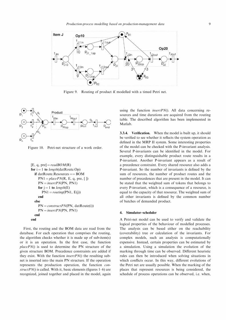
The PN structure in figure 9 is achieved if the sequence

of operations described by the routing table (table 2) is

modelled. The resulting PN structure is inserted into the

main PN model using the function insertPN().

The routings are sub-models that are inserted (by sub-

stitution, as defined previously) into the main model

defined by the BOM structure. However, some activities

of any sub-item may also be described with a BOM, i.e. in

the case they are composed of semi-products. The con-

struction of the overall Petri-net model can be achieved by

combining all of the intermediate steps.

3.3.3. Procedure for building the PN model. The work

order (WO) determines which and how many of the

finished products have to be produced. Each product can

be represented by a Petri-net model, shown in figure 7,

where one place is added in front and one at the end of the

structure to determine the start and end of the work. The

weight of the arc that connects tRin and pRin determines

the number of required products. To be able to consider

different starting times for different quantities of one

product the general structure shown in figure 10 is used.

The clocks, which are assigned to the tokens that are in

starting places, determine the starting time of every batch

of products.

The modelling procedure can be summarized by the

following algorithm:

Algorithm 1

[R, q, st]¼ readWO()

For i¼ 1 to length(R)

E¼ readBOM(R(i))

PN¼ placePN(R(i), E, q(i), [ ], st(i), x0, y0)

PN¼ routing(PN, R(i))

end

First, the data concerning the WO are read. The products

that are needed to be produced are given in R; in vector q

the quantities of the desired products are passed; and

vector st is used to determine the starting time of each

product. For each product the Petri-net structure, shown in

figure 10, is determined and placed in the model. The step

when the routing() is called is described in more detail by

algorithm 2:

Algorithm 2

function PN¼ routing(PN, R)

datRoute¼ readRouting(R)

Figure 8. BOM structure defined by PN.

Table 2. Routing of product K.

J Operations Duration Resources

Op10 10 s/9 s R1/R2

Op20 20 s R1, 3R3


[E, q, pre]¼ readBOM(R)

for i¼ 1 to length(datRoute.Op)

if datRoute.Resources¼¼BOM

PN1¼ placePN(R, E, q, pre, [ ])

PN¼ insertPN(PN, PN1)

for j¼ 1 to length(E)

PN1¼ routing(PN1, E(j))

end

else

PN¼ constructPN(PN, datRoute(i))

PN¼ insertPN(PN, PN1)

end

end

First, the routing and the BOM data are read from the

database. For each operation that comprises the routing,

the algorithm checks whether it is made up of sub-item(s)

or it is an operation. In the first case, the function

placePN() is used to determine the PN structure of the

given structure BOM. Precedence constraints are added if

they exist. With the function insertPN() the resulting sub-

net is inserted into the main PN structure. If the operation

represents the production operation, the function con-

structPN() is called. With it, basic elements (figures 1–6) are

recognized, joined together and placed in the model, again

using the function insertPN(). All data concerning re-

sources and time durations are acquired from the routing

table. The described algorithm has been implemented in

Matlab.

3.3.4. Verification. When the model is built up, it should

be verified to see whether it reflects the system operation as

defined in the MRP II system. Some interesting properties

of the model can be checked with the P-invariant analysis.

Several P-invariants can be identified in the model. For

example, every distinguishable product route results in a

P-invariant. Another P-invariant appears as a result of

a precedence constraint. Every shared resource also adds a

P-invariant. So the number of invariants is defined by the

sum of resources, the number of product routes and the

number of precedences that are present in the model. It can

be stated that the weighted sum of tokens that belongs to

every P-invariant, which is a consequence of a resource, is

equal to the capacity of that resource. The weighted sum of

all other invariants is defined by the common number

of batches of demanded product.

4. Simulator–scheduler

A Petri-net model can be used to verify and validate the

logical properties of the behaviour of modelled processes.

The analysis can be based either on the reachability

(coverability) tree or calculation of the invariants. For

complex models, such an analysis is computationally

expensive. Instead, certain properties can be estimated by

a simulation. Using a simulation the evolution of the

marking through time can be observed. Different heuristic

rules can then be introduced when solving situations in

which conflicts occur. In this way, different evolutions of

the Petri net are usually possible. When the marking of the

places that represent resources is being considered, the

schedule of process operations can be observed, i.e. when,

Figure 9. Routing of product K modelled with a timed Petri net.

Figure 10. Petri-net structure of a work order.


and using which resource, a job has to be processed.

Usually, different rules are needed to improve different

predefined production objectives (makespan, throughput,

production rates, and other temporal quantities).

To demonstrate the practical applicability of the

proposed modelling method for the purposes of scheduling

we built a simulator in Matlab that takes a Petri-net model

generated by the above algorithm. The simulator allows

different priority dispatching rules to be implemented. With

the simulation a marking trace of a timed Petri net can be

achieved. The marking trace of places that represent

resources is characterized as a schedule. The simulator is

able to deal with situations in which a conflict occurs, the

conflict being solved by a decision maker. By introducing

different heuristic dispatching rules (priority rules) deci-

sions can be made easily. In this way, only one path from

the reachability graph is calculated, which means that the

algorithm does not require a lot of computational effort.

Depending on the given scheduling problem a convenient

rule should be chosen.

The procedure of each simulation step computes a new

state skþ1¼ (mkþ1, nkþ1, rkþ1) of a timed Petri net in the

next calculation interval.

(i) Obtain the marking of the classical (untimed) Petri

net, i.e. only available tokens are considered.

Calculate the corresponding firing vector uk of

the untimed Petri net. At this point a conflict re-

solution is also applied.

. mk! uk.

(ii) If no transition is being fired (uk¼ 0), the time

passes on – the values of the local clocks are de-

creased by the value of the smallest local clock.

. Mk¼mkþ nk,

. Ts¼min pi2P(minl(rk(pi)[l])), r(pi) is not

empty,

. rkþ1(pi)¼ rk(pi)7Ts, 8r(pi)[l], 8 pi2P and r(pi)

is not empty – remove clocks for tokens that

became zero,

. nkþ1(pi)¼ dim(rkþ1(pi)), 8pi2P and r(pi) is not

empty,

. mkþ1¼Mk7 nkþ1.

(iii) In other cases (uk 6¼ 0), the time remains the same.

The firing vector uk defines the new state of the

timed Petri net, i.e. the distribution of tokens over

the places and the values of local clocks corre-

sponding to newly created tokens.

. Mk¼mkþ nk,

. Mkþ1¼Mkþ (O7 I) � uk,

. nkþ1(pi)¼ nk(pi)þO(pi, tj) � ukj, 8pi2P and 8tj2{t2T : f(t)4 0},

. rkþ1(pi)¼ rk(pi); rkþ1(pi)[h]¼ f(tj), for h¼ nk(pi)þ1, . . . ,nkþ1(pi),

. mkþ1¼Mkþ17 nkþ1.

In step (i) the firing vector uk is determined. In the case of

conflict it has to determine which transition to fire from

among all those that are enabled. Different heuristics can

be applied at this point. In step (ii), when no transitions are

enabled, first the sum of the available and unavailable

tokens is defined (Mk). Next the value of the smallest local

clock has to be recognized (Ts). The values of every clock

are then decreased for Ts. If the value of any clock becomes

zero, this clock has to be destroyed. As the number of

unavailable tokens has changed, vector n has to be

redefined in the next stage. Vector Mk can then be used

to determine mkþ1, as the number of tokens in a place does

not change. Step (iii) deals with the situation when firing

has to be performed as determined by firing vector uk.

Again, first the sum of the available and unavailable tokens

is defined (Mk). Firing vector uk determines the new

amount of all tokensMkþ1. The new number of unavailable

tokens can be calculated separately. In the next stage

the clocks for each token have to be determined rkþ1(pi).

While previous local clocks remain the same, new local

clocks have to be defined for every newly created token.

The initial state of the clock is determined by the delay of

the transition that created that token. The vector of

available tokens can now easily be determined from Mkþ1

and nkþ1.

The simulation is finished when there are no unavailable

tokens in the model or the global clock reaches the pre-

defined stop time.

In this algorithm the firing of the transitions is instan-

taneous. This is solved by the fact that time is not passed on

when any transition is enabled. It is assumed that the

situations where the enabling (firing) of a transition at

one time instant is cycling are prohibited. This kind

of situation would only occur in the case of incorrect

modelling.

After the simulation is finished the marking over time

can be observed. A Gantt chart can be produced if

evolution of the marking in the places that represent the

resources is observed. From the chart the schedule of the

modelled process can be obtained.

5. Case study: the production of furniture fittings

The applicability of our approach will be demonstrated on

a model of a production system where furniture fittings are

produced. The production system is divided into a number

of departments. The existing information-technology sys-

tems include a management system, which is used to plan

the production, and a supervisory system, which is used to

supervise the production process. To implement a detailed

schedule, how the work should be done, an additional

scheduling system should be implemented. The scheduling

can be performed using timed Petri nets. The data needed

to produce a Petri-net model can be retrieved from the


existing information systems. In the presented model, only

a small part of the production process will be considered.

The process under consideration is an assembly process

where different finished products are assembled from a

number of sub-items. During the production process,

different production facilities are used to produce sub-items

and finished products. The production facility considered in

this example is shown in figure 11. The process route of each

finished product starts with a punching machine. The

process continues through different resources, such as

assembly lines, a paint chamber, and galvanization lines.

At the final stage there is another assembly line where the

finished products are assembled and packed.

In the considered problem, four different types of pro-

ducts are produced: ‘Corner clamp L’, ‘Corner clamp R’,

‘Clamp holder’ and ‘Angle-bar’. The request for what and

how many products to produce is given by work orders.

Each work order also has its starting time. Table 3 lists the

work orders considered in our case.

Each product is composed of one or more sub-assembly

items. The structure of all products is described by the bill

of materials (table 4). When there are no precedence

constraints between sub-items, all the elements of the

precedence-constraints matrix are 0, and the matrix is

simply represented by [0].

To build a particular item from the BOM list, some

process steps are needed. These steps are described by

routing data and are given in tables 5–7. A description of

the data presented in the table will be given later during the

modelling procedure.

The final product of one production stage represents the

input material for the next stage. In this way the scheduling

procedure should ensure that work orders are timely

adjusted and thus ensure that, at each stage, sufficient

semi-products are produced. This kind of schedule is

feasible. Using different heuristic rules it is possible to

obtain a schedule that satisfies different objectives.

5.1. Modelling

Data from the BOM and the routings were used to build a

Petri-net model. The development of the model will be

presented for the part of the production where the left

corner clamp is produced. As we can see from table 3, there

are two work orders: the first has to start immediately with

its production, while the starting time of the second is 80

time units later. When we apply the first step of our

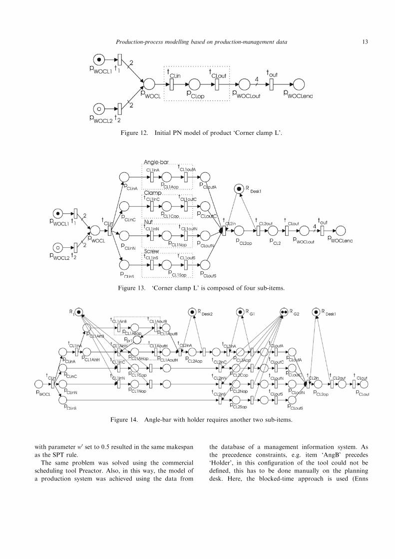
algorithm, the PN structure, shown in figure 12, is obtained.

The production of different amounts of products starts at

different times. Starting times are defined by the tokens in

the starting places pWOCL1 and pWOCL2, and the quantity of

each is defined by the weights of the corresponding arcs.

From table 5 the routing data concerning the product

‘Corner Clamp L’ (CL) are read. The first operation in this

table (Op1) shows that the sub-items should be produced

first as prescribed by ‘BOM_CCL’. This BOM is defined in

table 4, and, as we can see, four different sub-items are

needed (‘Angle-bar with holder L’, ‘Clamp’, ‘Nut’ and

‘Screw’). It is clear from the table that, for each item, a

designation character is given with its item name. These

characters are used in the Petri-net model to indicate the

item. When these subitems are produced, the production

proceeds with an assembly – Op2. This situation is demo-

nstrated by the Petri-net structure shown in figure 13.

In the following, the algorithm recognizes the routing

data for each of these sub-items. The routing data needed

to build the sub-items of a ‘Corner Clamp L’ are given in

table 5. There is one operation needed to produce the sub-

item ‘Screw’, two operations to produce ‘Nut’ and ‘Clamp’,

and three operations to produce the ‘Angle-bar with holder

L’. Using these data the structure as defined in figure 14 is

achieved. Some denotations of the transitions and places

are omitted to achieve a clearer representation of the

model. Also, the nodes that designate the start and end of

production are not shown.

Figure 11. Production plant.


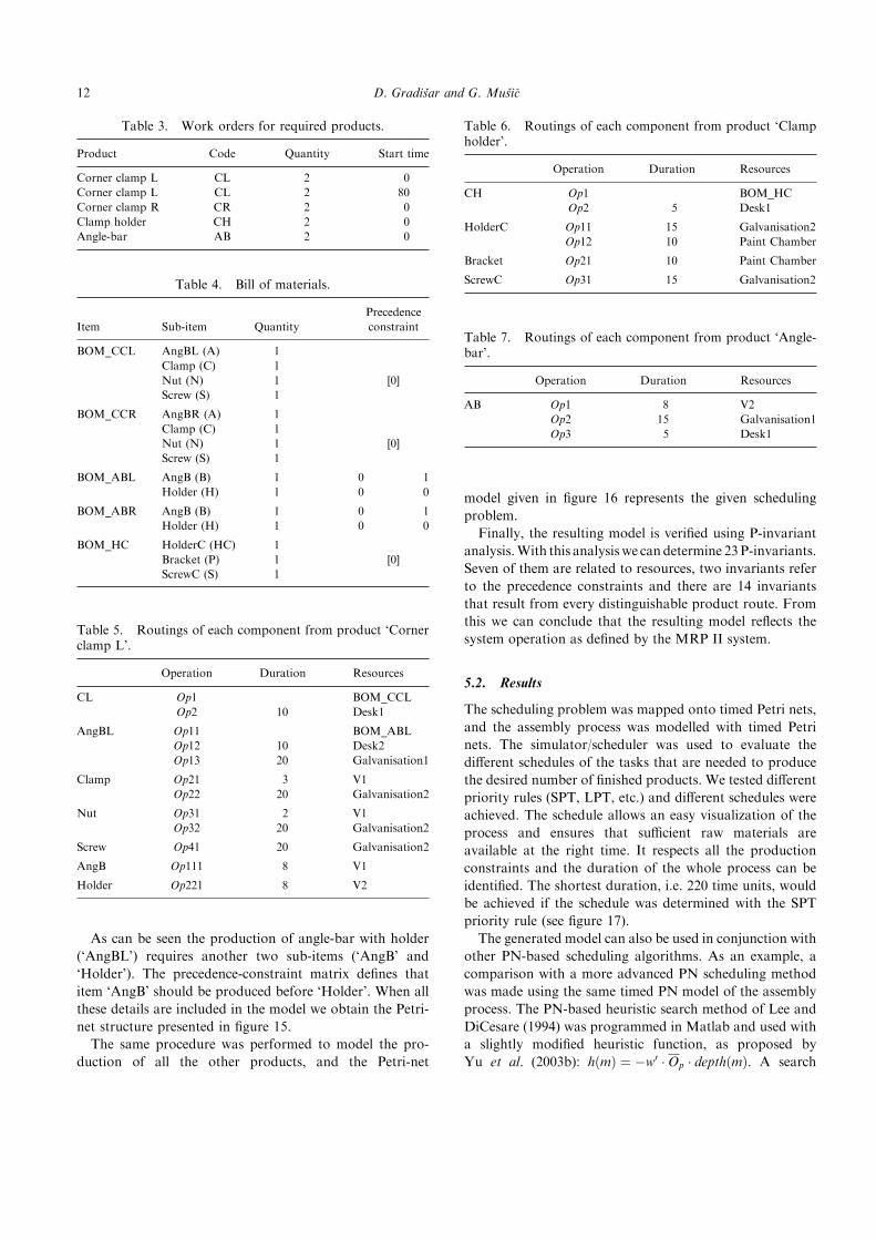
As can be seen the production of angle-bar with holder

(‘AngBL’) requires another two sub-items (‘AngB’ and

‘Holder’). The precedence-constraint matrix defines that

item ‘AngB’ should be produced before ‘Holder’. When all

these details are included in the model we obtain the Petri-

net structure presented in figure 15.

The same procedure was performed to model the pro-

duction of all the other products, and the Petri-net

model given in figure 16 represents the given scheduling

problem.

Finally, the resulting model is verified using P-invariant

analysis.With this analysiswe candetermine 23P-invariants.

Seven of them are related to resources, two invariants refer

to the precedence constraints and there are 14 invariants

that result from every distinguishable product route. From

this we can conclude that the resulting model reflects the

system operation as defined by the MRP II system.

5.2. Results

The scheduling problem was mapped onto timed Petri nets,

and the assembly process was modelled with timed Petri

nets. The simulator/scheduler was used to evaluate the

different schedules of the tasks that are needed to produce

the desired number of finished products. We tested different

priority rules (SPT, LPT, etc.) and different schedules were

achieved. The schedule allows an easy visualization of the

process and ensures that sufficient raw materials are

available at the right time. It respects all the production

constraints and the duration of the whole process can be

identified. The shortest duration, i.e. 220 time units, would

be achieved if the schedule was determined with the SPT

priority rule (see figure 17).

The generated model can also be used in conjunction with

other PN-based scheduling algorithms. As an example, a

comparison with a more advanced PN scheduling method

was made using the same timed PN model of the assembly

process. The PN-based heuristic search method of Lee and

DiCesare (1994) was programmed in Matlab and used with

a slightly modified heuristic function, as proposed by

Yu et al. (2003b): hðmÞ ¼ �w0 �Op � depthðmÞ. A search

Table 3. Work orders for required products.

Product Code Quantity Start time

Corner clamp L CL 2 0

Corner clamp L CL 2 80

Corner clamp R CR 2 0

Clamp holder CH 2 0

Angle-bar AB 2 0

Table 4. Bill of materials.

Item Sub-item Quantity

Precedence

constraint

BOM_CCL AngBL (A) 1

Clamp (C) 1

Nut (N) 1 [0]

Screw (S) 1

BOM_CCR AngBR (A) 1

Clamp (C) 1

Nut (N) 1 [0]

Screw (S) 1

BOM_ABL AngB (B) 1 0 1

Holder (H) 1 0 0

BOM_ABR AngB (B) 1 0 1

Holder (H) 1 0 0

BOM_HC HolderC (HC) 1

Bracket (P) 1 [0]

ScrewC (S) 1

Table 5. Routings of each component from product ‘Cornerclamp L’.

Operation Duration Resources

CL Op1 BOM_CCL

Op2 10 Desk1

AngBL Op11 BOM_ABL

Op12 10 Desk2

Op13 20 Galvanisation1

Clamp Op21 3 V1


Nut Op31 2 V1


Screw Op41 20 Galvanisation2

AngB Op111 8 V1

Holder Op221 8 V2

Table 6. Routings of each component from product ‘Clampholder’.


CH Op1 BOM_HC

Op2 5 Desk1

HolderC Op11 15 Galvanisation2

Op12 10 Paint Chamber

Bracket Op21 10 Paint Chamber

ScrewC Op31 15 Galvanisation2

Table 7. Routings of each component from product ‘Angle-bar’.


AB Op1 8 V2


Op3 5 Desk1


with parameter w0 set to 0.5 resulted in the same makespan

as the SPT rule.

The same problem was solved using the commercial

scheduling tool Preactor. Also, in this way, the model of

a production system was achieved using the data from

the database of a management information system. As

the precedence constraints, e.g. item ‘AngB’ precedes

‘Holder’, in this configuration of the tool could not be

defined, this has to be done manually on the planning

desk. Here, the blocked-time approach is used (Enns

Figure 12. Initial PN model of product ‘Corner clamp L’.

Figure 13. ‘Corner clamp L’ is composed of four sub-items.

Figure 14. Angle-bar with holder requires another two sub-items.


1996) to schedule jobs. In this way, all operations for a

selected job (order) are scheduled, starting with the first

operation and then forward in time to add later

operations. The next job is then loaded until all the

jobs have been done. The result using this tool is

presented in figure 18. From this Gantt chart we can see

that this schedule would finish the job in 238 time units

(table 8).

Figure 15. PN model of product ‘Corner clamp L’.

Figure 16. PN model of all products.


Figure 17. Schedule of the tasks in a production process using the SPT priority rule.

Figure 18. Schedule of the tasks in a production process using Preactor.


6. Conclusion

To be able to analyse a production system, a mathematical

model of the system is required. Timed Petri nets represent

a powerful mathematical formalism. In our work, timed

Petri nets with the holding-duration principle of time

implementation were used to automate the modelling of a

type of production system described by data from

production-management systems. The production data

are given with the BOM and the routings. The procedure

for building a model using these data is presented. For the

particular timed Petri net we present a simulator that can

be used to simulate models built with timed Petri nets. For

the purposes of scheduling, different heuristic rules can be

introduced into the simulator. The same timed Petri-net

model can also be used in conjunction with other Petri-net

scheduling algorithms, e.g. heuristic search. The applic-

ability of the proposed approach was illustrated for an

assembly process for producing furniture fittings. The

model developed with the proposed method was used to

determine a schedule for production operations. The results

were compared with a commercial scheduling tool. For

future work we plan to investigate the applicability of high-

level Petri nets to the proposed modelling method as well as

the use of the generated models for the testing of various

heuristic search algorithms.

References

Abdeddaim, Y., Asarin, E. and Maler, O., Scheduling with timed

automata. Theoretical Computer Science, 2006, 354, 272–300.

Arjona-Suarez, E. and Lopez-Mellado, E., Synthesis of coloured Petri nets

for FMS task specification. International Journal of Robotics and

Automation, 1996, 11, 111–117.

Basile, F., Chiacchio, P., Mazzocca, N. and Vittorini, V., Modeling and

control specification of flexible manufacturing systems using behavioral

traces and Petri nets building blocks. Journal of Intelligent Manufactur-

ing, to appear.

Blackstone, J.H., Phillips, D.T. and Hogg, G.L., A state-of-the-art survey

of dispatching rules for manufacturing job shop operations. International

Journal of Production Research, 1982, 20, 27–45.

Bła _zewicz, J., Domschke, W. and Pesch, E., The job shop scheduling

problem: conventional and new solution techniques. European Journal of

Operational Research, 1996, 93, 1–33.

Bła _zewicz, J., Pesch, E. and Sterna, M., The disjunctive graph machine

representation of the job shop scheduling problem. European Journal of

Operational Research, 2000, 127, 317–331.

Bowden, F.D.J., A brief survey and synthesis of the roles of time in Petri

nets. Mathematical & Computer Modelling, 2000, 31, 55–68.

Camurri, A., Franchi, P., Gandolfo, F. and Zaccaria, R., Petri net

based process scheduling: a model of the control system of flexible

manufacturing systems. Journal of Intelligent and Robotic Systems, 1993,

8, 99–123.

Czerwinski, C.S. and Luh, P.B., Scheduling products with bills of materials

using an improved Lagrangian relaxation technique. IEEE Transactions

on Robotics and Automation, 1994, 10, 99–111.

Enns, S.T., Finite capacity scheduling systems: performance issues

and comparisons. Computers and Industrial Engineering, 1996, 30,

727–739.

Ezpeleta, J. and Colom, J.M., Automatic synthesis of colored Petri nets for

the control of FMS. IEEE Transactions on Robotics and Automation,

1997, 13, 327–337.

Gu, T. and Bahri, P.A., A survey of Petri net applications in batch pro-

cesses. Computers in Industry, 2002, 47, 99–111.

Hauptman, B. and Jovan, V., An approach to process producion reactive

scheduling. ISA Transactions, 2004, 43, 305–318.

Huang, H.H., Lewis, F.L., Pastravanu, O.C. and Gurel, A., Flow shop

scheduling design in an FMS matrix framework. Control Engineering

Practice, 1995, 3, 561–568.

Jain, A.S. and Meeran, S., Deterministic job-shop scheduling: past,

present and future. European Journal of Operational Research, 1999, 113,

390–434.

Janneck, J.W. and Esser, R., Higher-order petri net modelling – techniques

and applications, in Formal Methods in Software Engineering and

Defence Systems. Conferences on Research and Practice in Information

Technology, 2002, pp. 17–25.

Jeng, M.D., A Petri net synthesis theory for modelling flexible manufactur-

ing systems. IEEE Transactions on Systems, Man, and Cybernetics – Part

B: Cybernetics, 1997, 27, 169–183.

Lee, D.Y. and DiCesare, F., Scheduling flexible manufacturing systems

using Petri nets and heuristic search. IEEE Transactions on Robotics and

Automation, 1994, 10, 123–132.

Lopez-Mellado, E., Analysis of discrete event systems by simulation of

timed Petri net models. Mathematics and Computers in Simulation, 2002,

61, 53–59.

Matcovschi, M.H., Mahuela, C. and Pastravanu, O., Petri net toolbox for

MATLAB, in 11th IEEE Mediterranean Conference on Control and

Automation, MED’03, 2003.

Murata, T., Properties, analysis and applications. Proceedings of the IEEE,

1989, 77, 541–580.

Panwalkar, S.S. and Iskaneder, W., A survey of Scheduling Rules.

Operations research, 1977, 25, 45–61.

Proth, J.M., Wang, L. and Xie, X., A class of Petri nets for manufacturing

system integration. IEEE Transactions on Robotics and Automation,

1997, 13, 317–326.

Ratzer, A., Wells, L., Lassen, H., Laursen, M., Qvortrup, J., Stissing, M.,

Westergaard, M., Christensen, S. and Jensen, K., CPN tools for editing,

simulating, and analysing coloured Petri nets, in 24th ICATPN, 2003,

pp. 450–462.

Recalde, L., Silva, M., Ezpeleta, J. and Teruel, E. In Petri Nets and

Manufacturing Systems: An Examples-Driven Tour, Lectures on

Concurrency and Petri Nets, Vol. 3098, pp. 742–788, 2004 (Springer:

Berlin).

Richard, P. and Proust, C., Solving scheduling problems using Petri nets

and constraint logic programming. RAIRO – Recherche Operationnelle –

Operations Research, 1998, 32, 125–143.

Silva, M. and Teruel, E., Petri nets for the design and operation of

manufacturing systems. European Journal of Control, 1997, 3, 82–

199.

Van der Aalst, W.M.P., Petri net based scheduling. OR Spectrum, 1996, 18,

219–229.

Table 8. Results.

Algorithm Time of execution

SPT rule 220

LPT rule 225

PN-based heuristic search 220

Preactor 238


Van der Aalst, W.M.P., The application of Petri nets to workflow

management. Journal of Circuits, Systems and Computers, 1998, 8,

21–66.

Wortmann, H., Comparison of information systems for engineer-to-order

and make-to-stock situations. Computers in Industry, 1995, 26, 261–

271.

Xue, Y., Kieckhafer, R.M. and Choobineh, F.F., Automated construction

of GSPN models for flexible manufacturing systems. Computers in

Industry, 1998, 37, 17–25.

Yeh, C.H., Schedule based production. International Journal of Production

Economics, 1997, 51, 235–242.

Yu, H., Reyes, A., Cang, S. and Lloyd, S., Combined Petri net modelling

and AI-based heuristic hybrid search for flexible manufacturing systems –

Part I: Petri net modelling and heuristic search. Computers and Industrial

Engineering, 2003, 44, 527–543.

Yu, H., Reyes, A., Cang, S. and Lloyd, S., Combined Petri net modelling

and AI-based heuristic hybrid search for flexible manufacturing

systems—Part II: Heuristic hybrid search. Computers and Industrial

Engineering, 2003, 44, 545–566.

Zhou, M., DiCesare, F. and Desrochers, A.A., A hybrid methodology for

synthesis of Petri net models for manufacturing systems. IEEE

Transactions on Robotics and Automation, 1992, 8, 350–361.

Zhou, M.C. and Venkatesh, K., Modelling, Simulation, and Control of

Flexible Manufacturing Systems: A Petri Net Approach, 1999 (World

Scientific: New York).

Zuberek, W.M., Timed Petri nets: definitions, properties and applications.

Microelectronics and Reliability, 1991, 31, 627–644.

Zuberek, W.M. and Kubiak, W., Timed Petri nets in modeling and analysis

of simple schedules for manufacturing cells. Computers and Mathematics

with Applications, 1999, 37, 191–206.


production-process modelling based on production ...msc.fe.uni-lj.si/papers/ijcim_gradisar.pdf ·...

Documents