1

Production and

Resource Use -

Supply Side

Chapters 3, 4, and 6

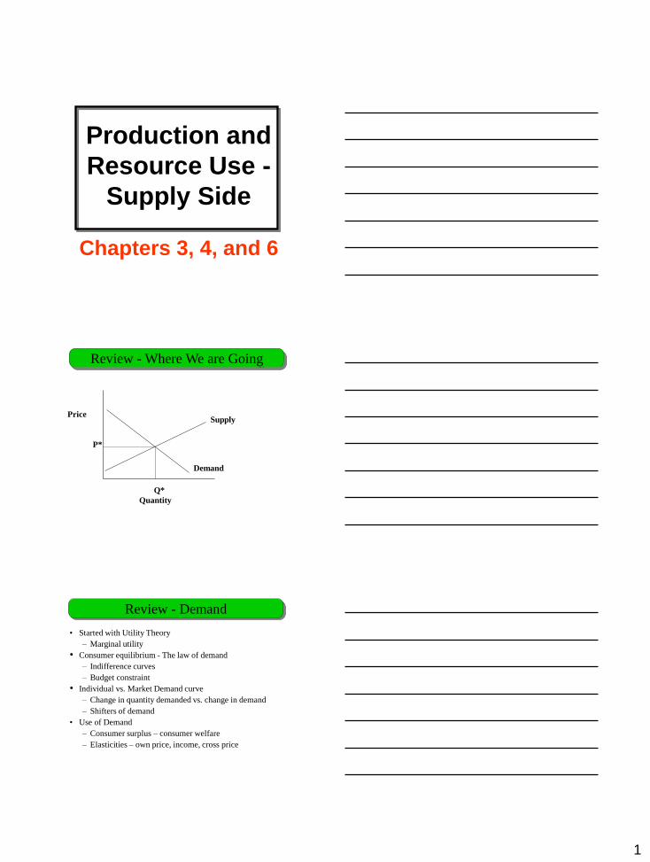
Review - Where We are Going

Q*

Quantity

Supply

Demand

Price

P*

Review - Demand

• Started with Utility Theory

– Marginal utility

• Consumer equilibrium - The law of demand

– Indifference curves

– Budget constraint

• Individual vs. Market Demand curve

– Change in quantity demanded vs. change in demand

– Shifters of demand

• Use of Demand

– Consumer surplus – consumer welfare

– Elasticities – own price, income, cross price

2

• Conditions of perfect competition

• Classification of inputs

• Important production relationships (for one variable input –TPP, APP, MPP)

• Assessing short run business costs (TC, AC,TVC, AVC, MC)

• Economics of short-run decisions

Topics of Discussion

• Expand production concepts to two inputs

• Concepts are analogous consumers

• Isoquants – Indifference curves

• MRTS – MRS

• Iso-cost lines - Budget constraint

• Least cost combinations – Consumer equilibrium

• Firm Specific

• Production Possibility Frontier

• Iso-revenue

• Long-run firm size

Topics of Discussion

• Homogeneous products

– Products from different producers are perfect

substitutes

• No barriers to entry or exit

– Resources are free to move in and out of the sector

• Large number of buyers and sellers

– No market power – price takers

• Perfect information

– Including quantities, prices, quality, sources of

resources etc.

Conditions for Perfect

Competition

3

• Land - includes renewable (forests) and non-

renewable (minerals) resources

• Labor - all owner and hired labor services,

excluding management

• Capital - manufactured goods such as fuel,

chemicals, tractors and buildings

• Management - production decisions

designed to achieve specific economic goal

Classification of Inputs

• Mathematical relationship that characterizes

the physical relationship between the use of

inputs and the level of outputs

What Are Production Functions?

Output = f(labor | capital, land, and

management)

Start with

one variable

input

Assume all other inputs

fixed at their current

levels…

Pickers

Corn

Dozen

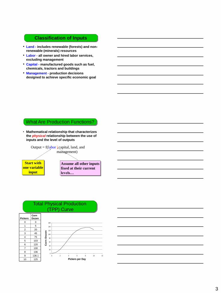
0 0

1 5

2 20

3 45

4 75

5 103

6 120

7 130

8 136

9 136.1

10 125

Total Physical Production

(TPP) Curve

0

20

40

60

80

100

120

140

160

0 2 4 6 8 10 12

Pickers per Day

Co

rn

Do

zen

4

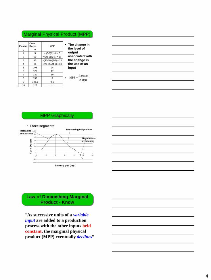
• The change in

the level of

output

associated with

the change in

the use of an

input

•

Pickers

Corn

Dozen MPP

0 0 --

1 5 = (5-0)/(1-0) = 5

2 20 =(20-5)/(2-1) = 15

3 45 =(45-20)/(3-2) = 25

4 75 =(75-45)/(4-3) = 30

5 103 28

6 120 17

7 130 10

8 136 6

9 136.1 0.1

10 125 -11.1

Marginal Physical Product (MPP)

input

outputMPP

-15

-10

-5

0

5

10

15

20

25

30

35

0 2 4 6 8 10 12

Pickers per Day

Co

rn D

oze

n

• Three segments

MPP Graphically

Increasing

and positive

Decreasing but positive

Negative and

decreasing

“As successive units of a variable

input are added to a production

process with the other inputs held

constant, the marginal physical

product (MPP) eventually declines”

Law of Diminishing Marginal

Product - Know

5

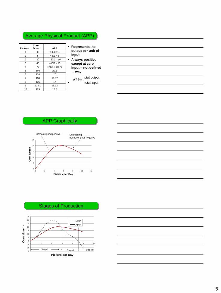
• Represents the

output per unit of

input

• Always positive

except at zero

input – not defined

– Why

•

Pickers

Corn

Dozen APP

0 0 = 0 /0 = --

1 5 = 5/1 = 5

2 20 = 20/2 = 10

3 45 =45/3 = 15

4 75 =75/4 = 18.75

5 103 20.6

6 120 20

7 130 18.57

8 136 17

9 136.1 15.12

10 125 12.5

Average Physical Product (APP)

inputtotal

outputtotalAPP

0

5

10

15

20

25

0 2 4 6 8 10 12

Pickers per Day

Co

rn D

ozen

APP Graphically

Increasing and positive Decreasing

but never goes negative

-15

-10

-5

0

5

10

15

20

25

30

35

0 2 4 6 8 10 12

Pickers per Day

Co

rn d

oze

n ~

MPP

APP

Stages of Production

Stage I Stage II Stage III

6

-15

-10

-5

0

5

10

15

20

25

30

35

0 2 4 6 8 10 12

Pickers per Day

Co

rn d

oze

n ~

0

20

40

60

80

100

120

140

160

0 2 4 6 8 10 12

Co

rn D

ozen

`

Stage IIIStage IIStage I

0

20

40

60

80

100

120

140

160

0 2 4 6 8 10 12

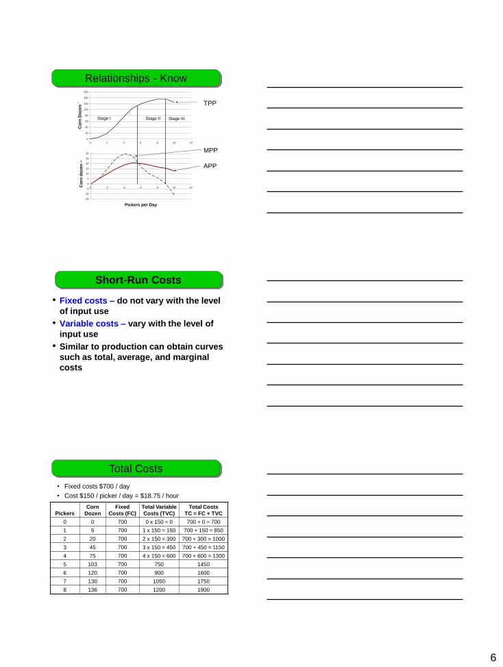
Relationships - Know

TPP

MPP

APP

• Fixed costs – do not vary with the level

of input use

• Variable costs – vary with the level of

input use

• Similar to production can obtain curves

such as total, average, and marginal

costs

Short-Run Costs

Pickers

Corn

Dozen

Fixed

Costs (FC)

Total Variable

Costs (TVC)

Total Costs

TC = FC + TVC

0 0 700 0 x 150 = 0 700 + 0 = 700

1 5 700 1 x 150 = 150 700 + 150 = 850

2 20 700 2 x 150 = 300 700 + 300 = 1000

3 45 700 3 x 150 = 450 700 + 450 = 1150

4 75 700 4 x 150 = 600 700 + 600 = 1300

5 103 700 750 1450

6 120 700 900 1600

7 130 700 1050 1750

8 136 700 1200 1900

Total Costs

• Fixed costs $700 / day

• Cost $150 / picker / day = $18.75 / hour

7

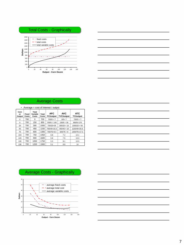
Total Costs - Graphically

0

200

400

600

800

1000

1200

1400

1600

1800

2000

0 20 40 60 80 100 120 140 160

Output - Corn Dozen

Do

llars

fixed costs

total costs

total variable costs

Corn

or

Output

Fixed

Costs

Total

Variable

Costs

Total

Costs

AFC FC/output

AVC TVC/output

ATC TC/output

0 700 0 700 700/0 = ? 0/0= ? 700/0 = ?

5 700 150 850 700/5 = 140 150/5 = 30 850/5=170

20 700 300 1000 700/20=35 300/20 = 15 1000/20 = 50

45 700 450 1150 700/45=15.5 450/45 = 10 1150/45=25.6

75 700 600 1300 700/75=9.3 600/75 = 8 1300/75=17.3

103 700 750 1450 6.8 7.2 14.1

120 700 900 1600 5.8 7.5 13.3

130 700 1050 1750 5.3 8.1 13.5

136 700 1200 1900 5.1 8.8 14

Average Costs

• Average = cost of interest / output

Average Costs - Graphically

0

10

20

30

40

50

60

0 20 40 60 80 100 120 140 160

Output - Corn Dozen

Do

llars

average fixed costs

average total cost

average variable costs

8

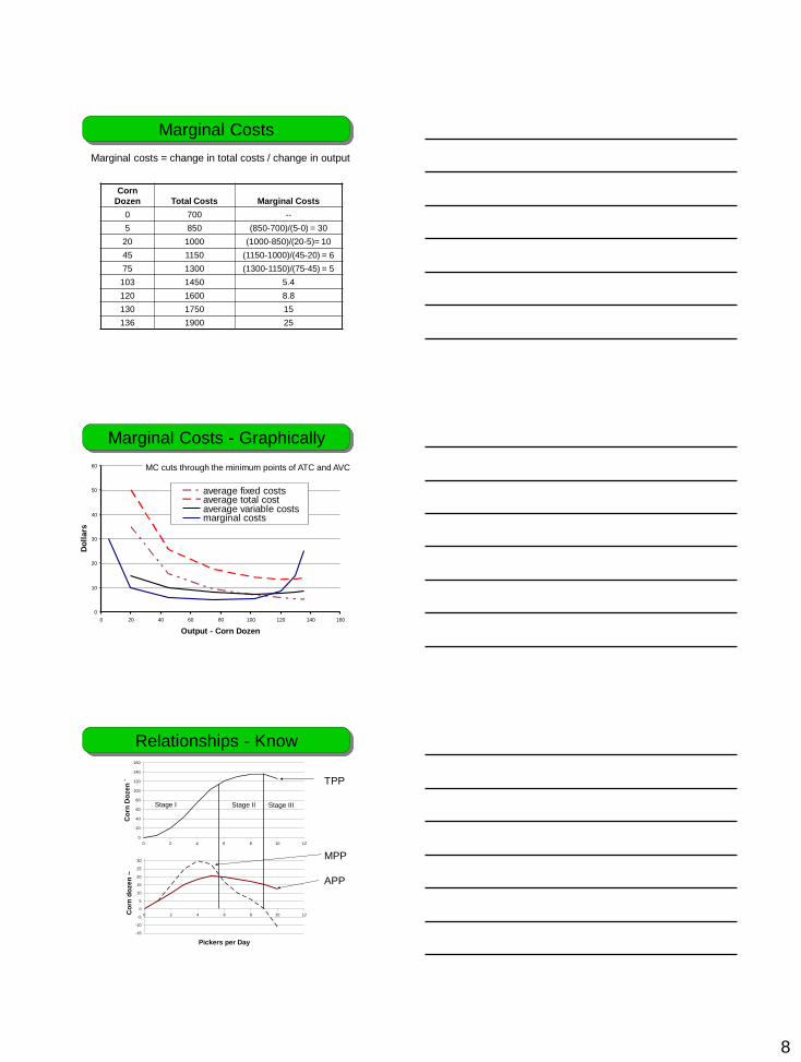
Corn

Dozen Total Costs Marginal Costs

0 700 --

5 850 (850-700)/(5-0) = 30

20 1000 (1000-850)/(20-5)= 10

45 1150 (1150-1000)/(45-20) = 6

75 1300 (1300-1150)/(75-45) = 5

103 1450 5.4

120 1600 8.8

130 1750 15

136 1900 25

Marginal Costs

Marginal costs = change in total costs / change in output

Marginal Costs - Graphically

0

10

20

30

40

50

60

0 20 40 60 80 100 120 140 160

Output - Corn Dozen

Do

llars

average fixed costsaverage total costaverage variable costsmarginal costs

MC cuts through the minimum points of ATC and AVC

-15

-10

-5

0

5

10

15

20

25

30

35

0 2 4 6 8 10 12

Pickers per Day

Co

rn d

oze

n ~

0

20

40

60

80

100

120

140

160

0 2 4 6 8 10 12

Co

rn D

ozen

`

Stage IIIStage IIStage I

0

20

40

60

80

100

120

140

160

0 2 4 6 8 10 12

Relationships - Know

TPP

MPP

APP

9

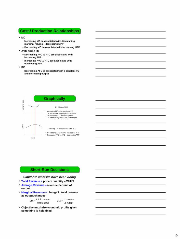
• MC

– Increasing MC is associated with diminishing

marginal returns – decreasing MPP

– Decreasing MC is associated with increasing MPP

• AVC and ATC

– Decreasing AVC & ATC are associated with

increasing APP

– Increasing AVC & ATC are associated with

decreasing APP

• FC

– Decreasing AFC is associated with a constant FC

and increasing output

Cost / Production Relationships

Input

Ma

rgin

al co

st

Ou

tpu

t

U – Shaped MC

• Increasing MC – decreasing MPP

Increasing output per unit of input

• Decreasing MC - increasing MPP

Decreasing output per unit of input

Similarly – U Shaped AVC and ATC

• Decreasing ATC or AVC - increasing APP

• Increasing ATC or AVC – decreasing APP

Graphically

Similar to what we have been doing

• Total Revenue = price x quantity – WHY?

• Average Revenue – revenue per unit of

output

• Marginal Revenue – change in total revenue

as output changes

• Objective maximize economic profits given

something is held fixed

Short-Run Decisions

output

revenueMR

outputtotal

revenuetotalAR

10

Corn

Dozen TC MC

Total Revenue

P x Q MR

Economic Profit

TR - TC

0 700 0 x 20 = 0 0 – 700 = -700

5 850 30 5 x 20 = 100 (100-0)/(5-0)

= 20 100 - 850 = -750

20 1000 10 20 x 20 = 400 (400-100)/(20-5)

=20 400 - 1000 = -600

45 1150 6 45 x 20 = 900 20 900 – 1150 = -250

75 1300 5 75 x 20 = 1500 20 1500 – 1300 = 200

103 1450 5.4 2060 20 610

120 1600 8.8 2400 20 800

130 1750 15 2600 20 850

136 1900 25 2720 20 820

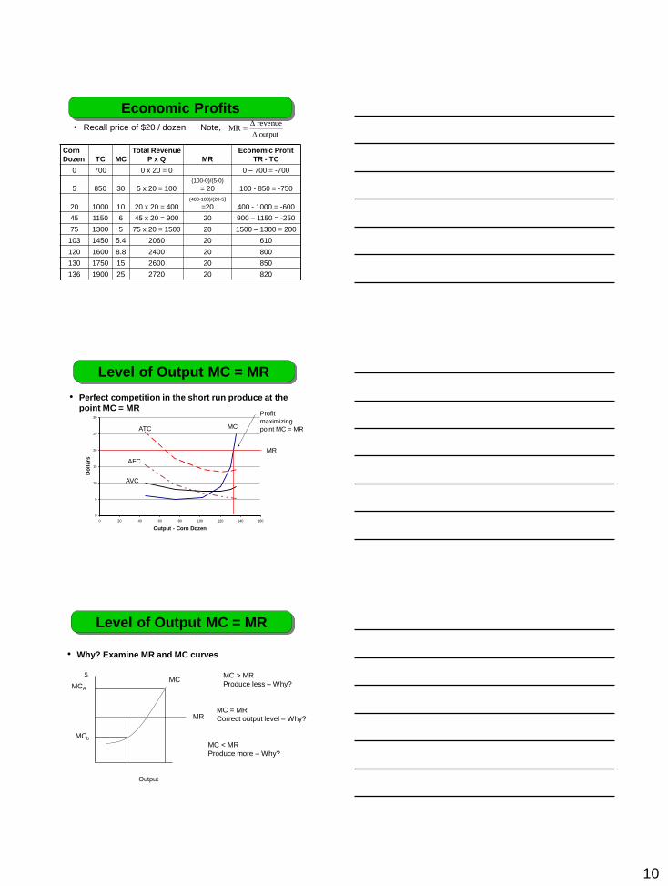
Economic Profits

• Recall price of $20 / dozen Note, output

revenueMR

0

5

10

15

20

25

30

0 20 40 60 80 100 120 140 160

Output - Corn Dozen

Do

llars

0

• Perfect competition in the short run produce at the

point MC = MR

Level of Output MC = MR

ATC

AFC

AVC

MC

Profit

maximizing

point MC = MR

MR

• Why? Examine MR and MC curves

Level of Output MC = MR

MC

MR

MCb

MCA

MC < MR

Produce more – Why?

MC > MR

Produce less – Why?

MC = MR

Correct output level – Why?

Output

$

11

Corn

Dozen TC MC

Total

Revenue MR

Economic Profit

TR - TC

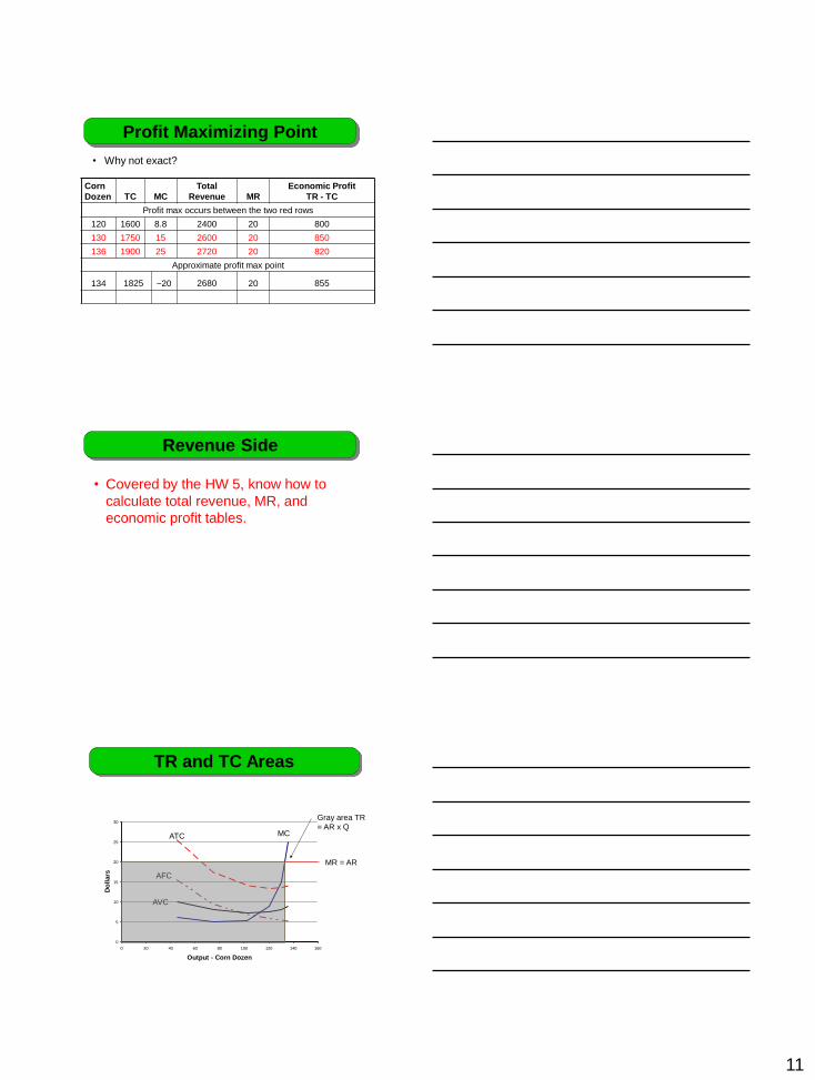
Profit max occurs between the two red rows

120 1600 8.8 2400 20 800

130 1750 15 2600 20 850

136 1900 25 2720 20 820

Approximate profit max point

134 1825 ~20 2680 20 855

Profit Maximizing Point

• Why not exact?

Revenue Side

• Covered by the HW 5, know how to

calculate total revenue, MR, and

economic profit tables.

0

5

10

15

20

25

30

0 20 40 60 80 100 120 140 160

Output - Corn Dozen

Do

llars

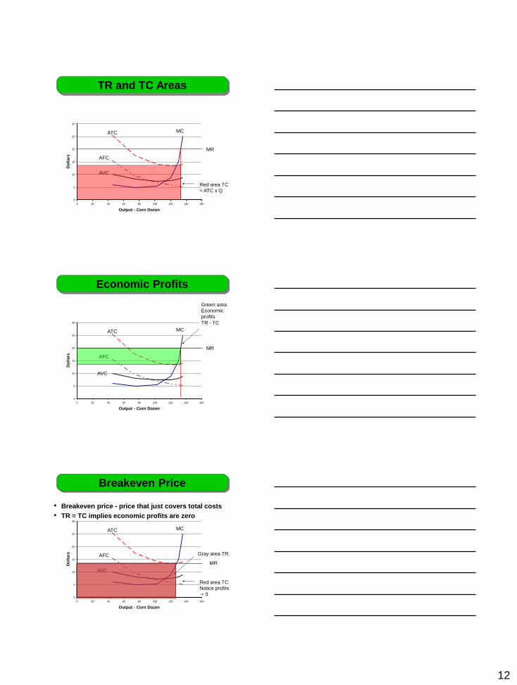
TR and TC Areas

ATC

AFC

AVC

MC

Gray area TR

= AR x Q

MR = AR

12

0

5

10

15

20

25

30

0 20 40 60 80 100 120 140 160

Output - Corn Dozen

Do

llars

TR and TC Areas

ATC

AFC

AVC

MC

MR

Red area TC

= ATC x Q

0

5

10

15

20

25

30

0 20 40 60 80 100 120 140 160

Output - Corn Dozen

Do

llars

Economic Profits

ATC

AFC

AVC

MC

Green area

Economic

profits

TR - TC

MR

0

5

10

15

20

25

30

0 20 40 60 80 100 120 140 160

Output - Corn Dozen

Do

llars

• Breakeven price - price that just covers total costs

• TR = TC implies economic profits are zero

Breakeven Price

ATC

AFC

AVC

MC

Gray area TR

Red area TC

Notice profits

= 0

MR

13

0

5

10

15

20

25

30

0 20 40 60 80 100 120 140 160

Output - Corn Dozen

Do

llars

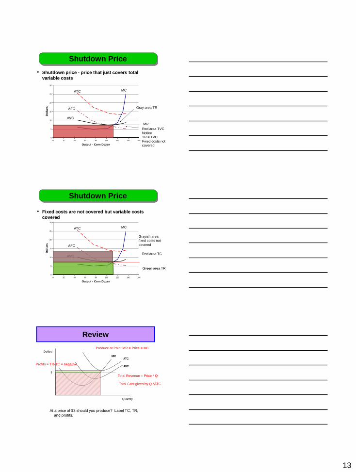
• Shutdown price - price that just covers total

variable costs

Shutdown Price

ATC

AFC

AVC

MC

Gray area TR

Red area TVC

Notice

TR = TVC

Fixed costs not

covered

MR

0

5

10

15

20

25

30

0 20 40 60 80 100 120 140 160

Output - Corn Dozen

Do

llars

• Fixed costs are not covered but variable costs

covered

Shutdown Price

ATC

AFC

AVC

MC

Grayish area

fixed costs not

covered

Red area TC

Green area TR

Review

At a price of $3 should you produce? Label TC, TR,

and profits.

MC ATC

AVC

Quantity

3

MC ATC

AVC

Dollars Produce at Point MR = Price = MC

Total Revenue = Price * Q

Total Cost given by Q *ATC

Profits = TR-TC = negative

14

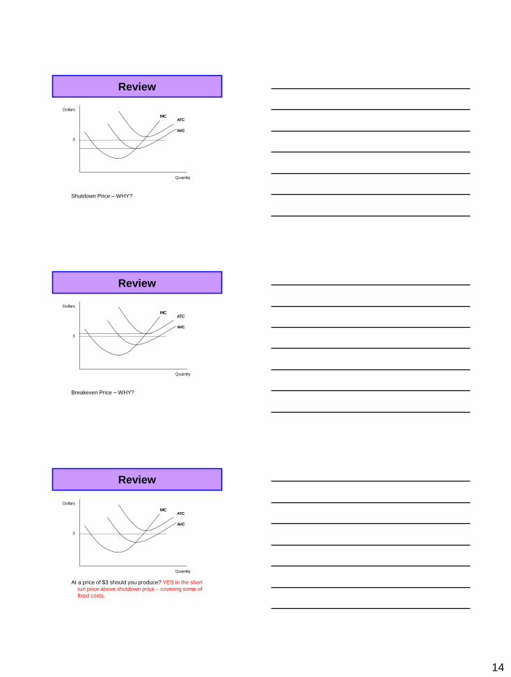
Review

Shutdown Price – WHY?

MC ATC

AVC

Quantity

3

MC ATC

AVC

Dollars

Review

Breakeven Price – WHY?

MC ATC

AVC

Quantity

3

MC ATC

AVC

Dollars

Review

At a price of $3 should you produce? YES in the short

run price above shutdown price – covering some of

fixed costs.

MC ATC

AVC

Quantity

3

MC ATC

AVC

Dollars

15

0

5

10

15

20

25

30

0 20 40 60 80 100 120 140 160

Output - Corn Dozen

Do

llars

• MC curve above the AVC

Firm’s Short-Run Supply Curve

ATC

AFC

AVC

MC

Own-Price Elasticity of Supply

• Measures the relationship between change in

quantity supplied and a change in price

Own-price

Elasticity

of Supply Percentage change in own price

Percentage change in quantity supplied =

]2/)P+P[()P-P(

]2/)Q+Q[()Q-Q(

=

BA

BA

SBSA

SBSA

Own-Price Elasticity of Supply

• Positive – Why?

If the elasticity is Supply is % in quantity is

Greater than 1.0 Elastic Greater than % in price

Less than 1.0 Inelastic Less as % in price

Equal to 1.0 Unitary Equal to % in price

Equal to 0 Perfectly

inelastic

Zero

Vertical supply curve

Equal to positive

infinity

Perfectly

elastic

% in price = zero

Horizontal supply curve

16

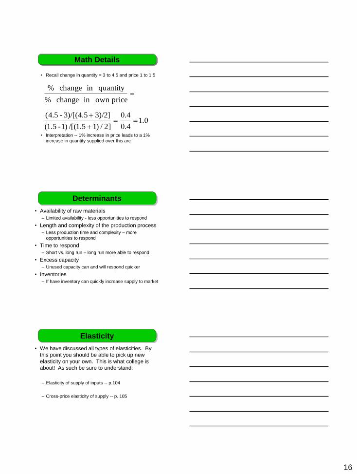
• Recall change in quantity = 3 to 4.5 and price 1 to 1.5

• Interpretation -- 1% increase in price leads to a 1%

increase in quantity supplied over this arc

Math Details

1.0 0.4

0.4

]2/)15.1/[()1 -5.1(

)/2]33)/[(4.5-5.4(

priceowninchange%

quantityinchange%

Determinants

• Availability of raw materials

– Limited availability - less opportunities to respond

• Length and complexity of the production process

– Less production time and complexity – more

opportunities to respond

• Time to respond

– Short vs. long run – long run more able to respond

• Excess capacity

– Unused capacity can and will respond quicker

• Inventories

– If have inventory can quickly increase supply to market

Elasticity

• We have discussed all types of elasticities. By

this point you should be able to pick up new

elasticity on your own. This is what college is

about! As such be sure to understand:

– Elasticity of supply of inputs -- p.104

– Cross-price elasticity of supply -- p. 105

17

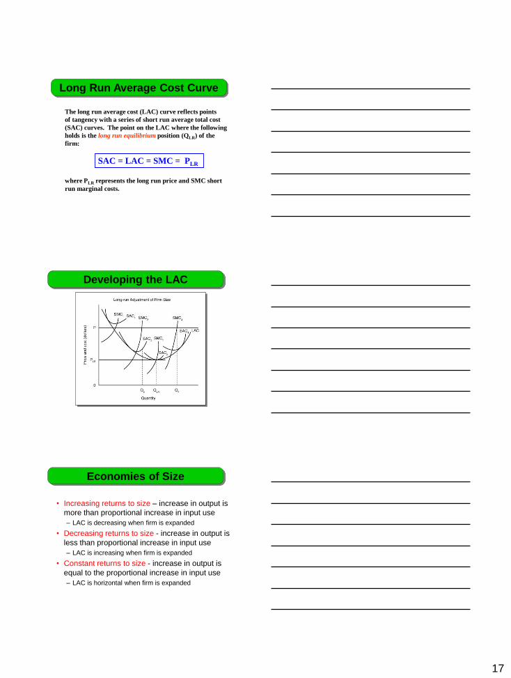
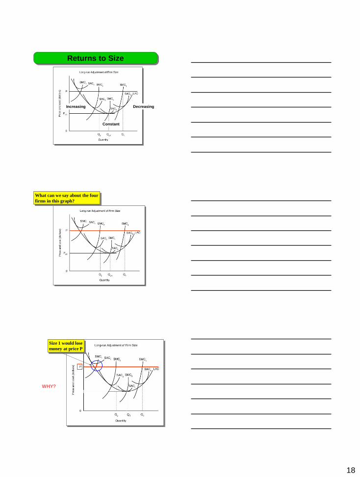
The long run average cost (LAC) curve reflects points

of tangency with a series of short run average total cost

(SAC) curves. The point on the LAC where the following

holds is the long run equilibrium position (QLR) of the

firm:

SAC = LAC = SMC = PLR

where PLR represents the long run price and SMC short

run marginal costs.

Long Run Average Cost Curve

Developing the LAC

• Increasing returns to size – increase in output is

more than proportional increase in input use

– LAC is decreasing when firm is expanded

• Decreasing returns to size - increase in output is

less than proportional increase in input use

– LAC is increasing when firm is expanded

• Constant returns to size - increase in output is

equal to the proportional increase in input use

– LAC is horizontal when firm is expanded

Economies of Size

18

Returns to Size

Decreasing Increasing

Constant

What can we say about the four

firms in this graph?

Q3

WHY?

Size 1 would lose

money at price P

19

Q3

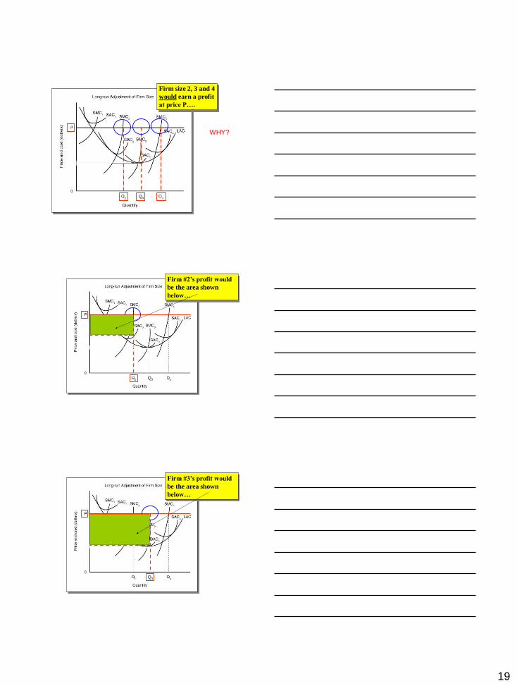
Firm size 2, 3 and 4

would earn a profit

at price P….

WHY?

Q3

Firm #2’s profit would

be the area shown

below…

Q3

Firm #3’s profit would

be the area shown

below…

20

Q3

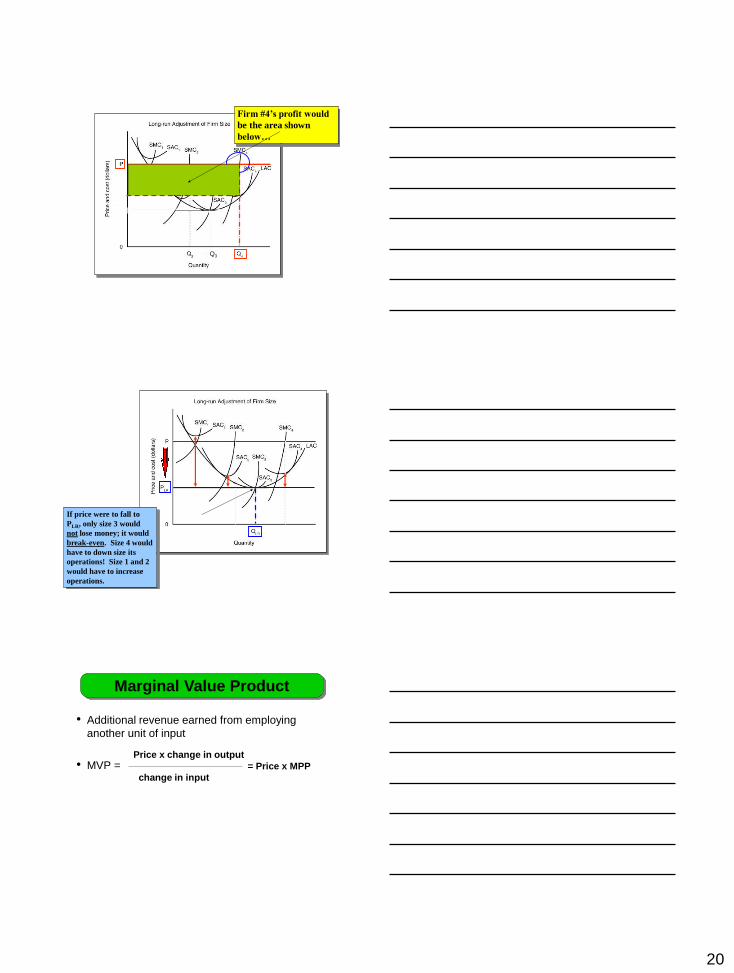
Firm #4’s profit would

be the area shown

below…

If price were to fall to

PLR, only size 3 would

not lose money; it would

break-even. Size 4 would

have to down size its

operations! Size 1 and 2

would have to increase

operations.

• Additional revenue earned from employing

another unit of input

• MVP =

Marginal Value Product

Price x change in output

= Price x MPP

change in input

21

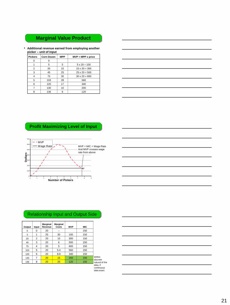
• Additional revenue earned from employing another

picker – unit of input

Marginal Value Product

Pickers Corn Dozen MPP MVP = MPP x price

0 0

1 5 5 5 x 20 = 100

2 20 15 15 x 20 = 300

3 45 25 25 x 20 = 500

4 75 30 30 x 20 = 600

5 103 28 560

6 120 17 340

7 130 10 200

8 136 6 120

0

100

200

300

400

500

600

700

0 1 2 3 4 5 6 7 8 9

Number of Pickers

Do

lla

rs

MVP

Wage Rate

Profit Maximizing Level of Input

MVP = MIC = Wage Rate

And MVP crosses wage

rate from above

Output Input

Marginal

Revenue

Marginal

Costs MVP MIC

0 0 20 -- 150

5 1 20 30 100 150

20 2 20 10 300 150

45 3 20 6 500 150

75 4 20 5 600 150

103 5 20 5.4 560 150

120 6 20 8.8 340 150

130 7 20 15 200 150

136 8 20 25 120 150

Relationship Input and Output Side

Within

discrete

natural of the

data, if

continuous

data exact.

22

• Exam one will cover all material to this point

Exam One to this point

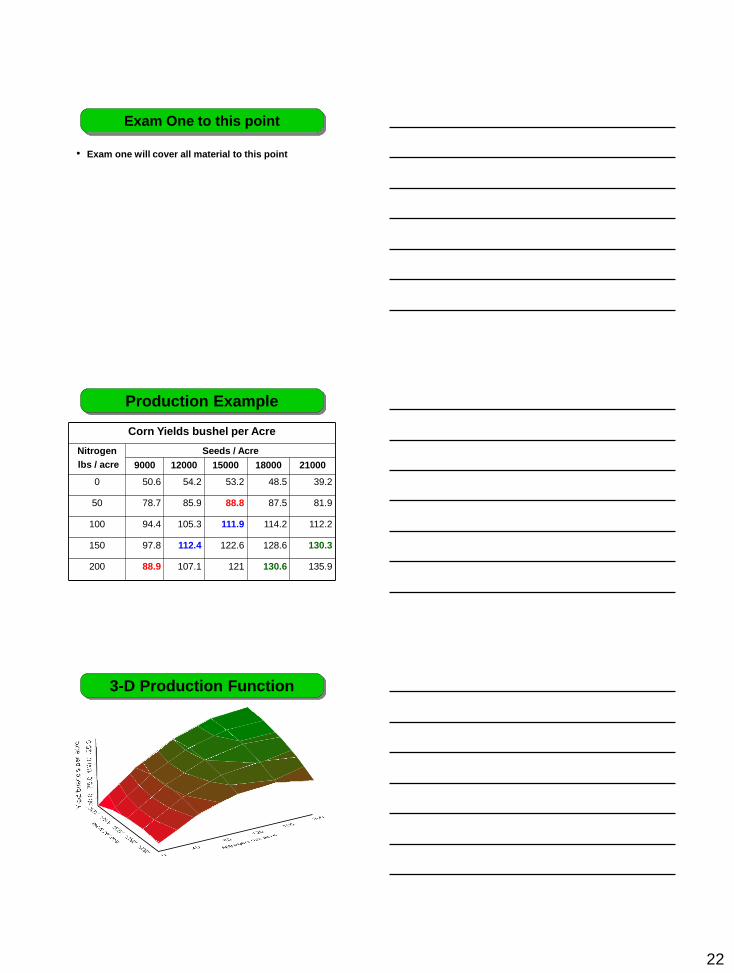
Production Example

Corn Yields bushel per Acre

Nitrogen

lbs / acre

Seeds / Acre

9000 12000 15000 18000 21000

0 50.6 54.2 53.2 48.5 39.2

50 78.7 85.9 88.8 87.5 81.9

100 94.4 105.3 111.9 114.2 112.2

150 97.8 112.4 122.6 128.6 130.3

200 88.9 107.1 121 130.6 135.9

3-D Production Function

23

0

5000

10000

15000

20000

25000

0 50 100 150 200 250Nitrogen per Acre

Seed

s p

er

Acre

.

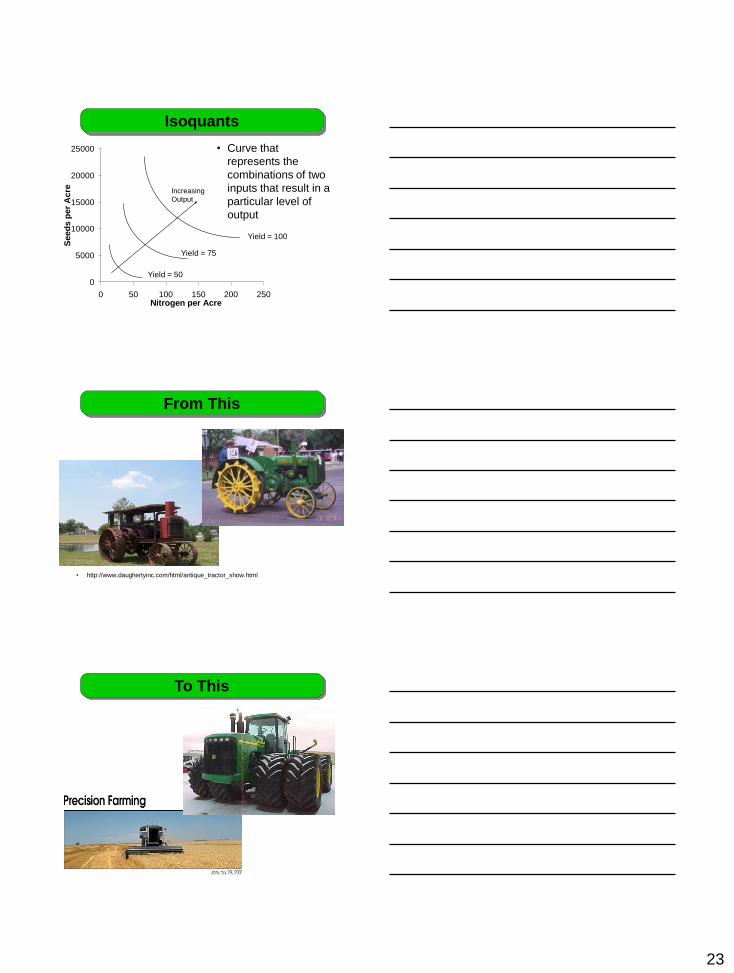
Yield = 100

Yield = 75

Yield = 50

Increasing

Output

Isoquants

• Curve that

represents the

combinations of two

inputs that result in a

particular level of

output

• http://www.daughertyinc.com/html/antique_tractor_show.html

From This

To This

24

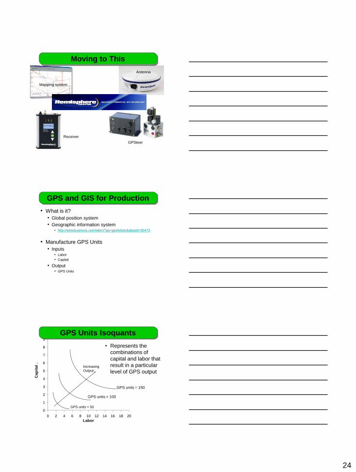
GPSteer

Mapping system

Antenna

Receiver

Moving to This

• What is it?

• Global position system

• Geographic information system • http://winebusiness.com/wbm/?go=getArticle&dataId=30473

• Manufacture GPS Units

• Inputs • Labor

• Capital

• Output • GPS Units

GPS and GIS for Production

0

1

2

3

4

5

6

7

8

9

10

0 2 4 6 8 10 12 14 16 18 20

Labor

Cap

ital

.

GPS units = 150

GPS units = 100

GPS units = 50

Increasing

Output

GPS Units Isoquants

• Represents the

combinations of

capital and labor that

result in a particular

level of GPS output

25

0

1

2

3

4

5

6

7

8

9

10

0 1 2 3 4 5 6 7 8 9 10

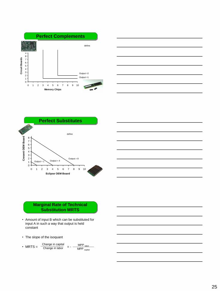
Memory Chips

Cir

cu

it B

oa

rds

Perfect Complements

define

Output =2

Output =1

0

1

2

3

4

5

6

7

8

9

10

0 1 2 3 4 5 6 7 8 9 10

Eclipse OEM Board

Cre

sen

t O

EM

Bo

ard

`

Perfect Substitutes

define

Output = 4 Output = 8

Output = 1

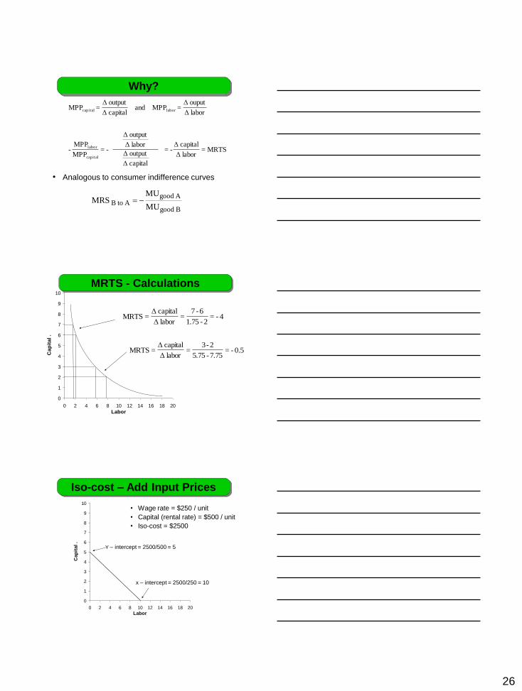
Marginal Rate of Technical

Substitution MRTS

• Amount of input B which can be substituted for

input A in such a way that output is held

constant

• The slope of the isoquant

• MRTS = = -

Change in capital

Change in labor MPP labor

MPP capital

26

• Analogous to consumer indifference curves

Why?

Bgood

AgoodAtoB

MU

MUMRS

MRTS=laborΔ

capitalΔ-=

capitalΔ

outputΔ

laborΔ

outputΔ

-=MPP

MPP-

laborΔ

ouputΔ=MPPand

capitalΔ

outputΔ=MPP

capital

labor

laborcapital

0

1

2

3

4

5

6

7

8

9

10

0 2 4 6 8 10 12 14 16 18 20

Labor

Cap

ital

.

MRTS - Calculations

4 -=2-1.75

6-7=

laborΔ

capitalΔ=MRTS

5.0 -=7.75-5.75

2-3=

laborΔ

capitalΔ=MRTS

Iso-cost – Add Input Prices

0

1

2

3

4

5

6

7

8

9

10

0 2 4 6 8 10 12 14 16 18 20

Labor

Ca

pit

al

.

Y – intercept = 2500/500 = 5

• Wage rate = $250 / unit

• Capital (rental rate) = $500 / unit

• Iso-cost = $2500

x – intercept = 2500/250 = 10

27

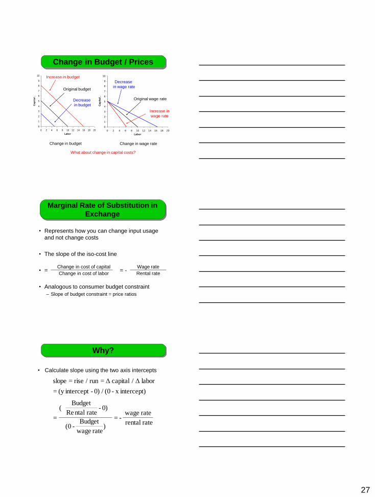
Change in Budget / Prices

0

1

2

3

4

5

6

7

8

9

10

0 2 4 6 8 10 12 14 16 18 20

Labor

Ca

pit

al

.

Increase in budget

Change in budget

Original budget

Decrease

in budget

0

1

2

3

4

5

6

7

8

9

10

0 2 4 6 8 10 12 14 16 18 20

Labor

Ca

pit

al

.

Change in wage rate

Increase in

wage rate

Original wage rate

Decrease

in wage rate

What about change in capital costs?

Marginal Rate of Substitution in

Exchange

• Represents how you can change input usage

and not change costs

• The slope of the iso-cost line

• = = -

• Analogous to consumer budget constraint

– Slope of budget constraint = price ratios

Change in cost of capital

Change in cost of labor

Wage rate

Rental rate

• Calculate slope using the two axis intercepts

Why?

raterental

ratewage- =

)rate wage

Budget - 0(

0) - ratentalRe

Budget(

=

intercept) x - (0 / 0) -intercept (y =

laborΔ/capitalΔ =run/rise = slope

28

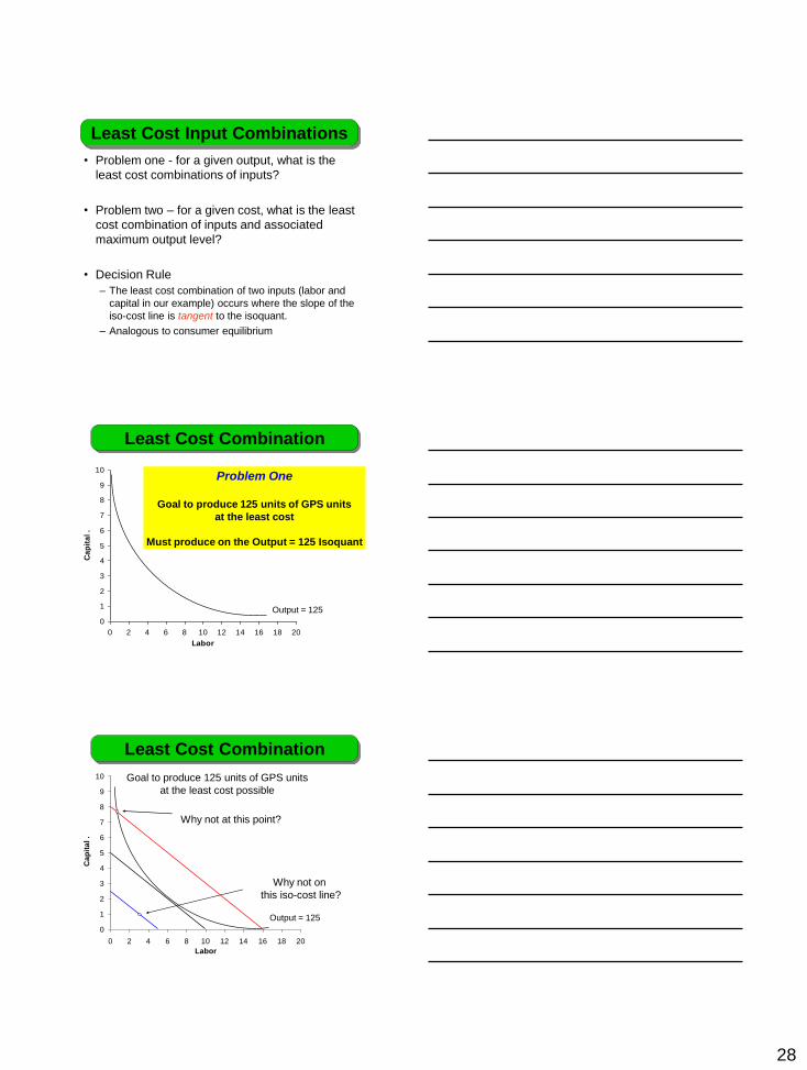
• Problem one - for a given output, what is the

least cost combinations of inputs?

• Problem two – for a given cost, what is the least

cost combination of inputs and associated

maximum output level?

• Decision Rule

– The least cost combination of two inputs (labor and

capital in our example) occurs where the slope of the

iso-cost line is tangent to the isoquant.

– Analogous to consumer equilibrium

Least Cost Input Combinations

0

1

2

3

4

5

6

7

8

9

10

0 2 4 6 8 10 12 14 16 18 20

Labor

Ca

pit

al

.

Least Cost Combination

Output = 125

Problem One

Goal to produce 125 units of GPS units

at the least cost

Must produce on the Output = 125 Isoquant

0

1

2

3

4

5

6

7

8

9

10

0 2 4 6 8 10 12 14 16 18 20

Labor

Ca

pit

al

.

Least Cost Combination

Output = 125

Goal to produce 125 units of GPS units

at the least cost possible

Why not at this point?

Why not on

this iso-cost line?

29

0

1

2

3

4

5

6

7

8

9

10

0 2 4 6 8 10 12 14 16 18 20

Labor

Ca

pit

al

.

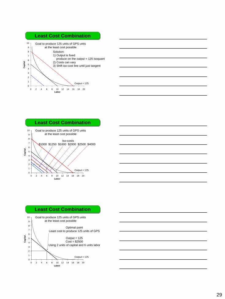
Least Cost Combination

Output = 125

Goal to produce 125 units of GPS units

at the least cost possible

Solution:

1) Output is fixed

produce on the output = 125 isoquant

2) Costs can vary

3) Shift iso-cost line until just tangent

0

1

2

3

4

5

6

7

8

9

10

0 2 4 6 8 10 12 14 16 18 20

Labor

Ca

pit

al

.

Least Cost Combination

Output = 125

Goal to produce 125 units of GPS units

at the least cost possible

Iso-costs

$1000 $1250 $1600 $2000 $2500 $4000

0

1

2

3

4

5

6

7

8

9

10

0 2 4 6 8 10 12 14 16 18 20

Labor

Ca

pit

al

.

Least Cost Combination

Output = 125

Goal to produce 125 units of GPS units

at the least cost possible

Optimal point

Least cost to produce 125 units of GPS

Output = 125

Cost = $2500

Using 2 units of capital and 6 units labor

30

0

1

2

3

4

5

6

7

8

9

10

0 2 4 6 8 10 12 14 16 18 20

Labor

Ca

pit

al

.

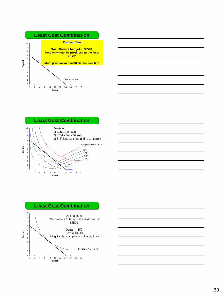
Least Cost Combination

Cost = $3500

Problem Two

Goal: Given a budget of $3500,

how much can be produced at the least

cost?

Must produce on the $3500 Iso-cost line

0

1

2

3

4

5

6

7

8

9

10

0 2 4 6 8 10 12 14 16 18 20

Labor

Ca

pit

al

.

Least Cost Combination

Output – GPS Units

175

150

125

100

25

Solution:

1) Costs are fixed

2) Production can vary

3) Shift isoquant line until just tangent

0

1

2

3

4

5

6

7

8

9

10

0 2 4 6 8 10 12 14 16 18 20

Labor

Ca

pit

al

.

Least Cost Combination

Optimal point

Can produce 150 units at a least cost of

$3500

Output = 150

Cost = $3500

Using 3 units of capital and 8 units labor

Output = 150 units

31

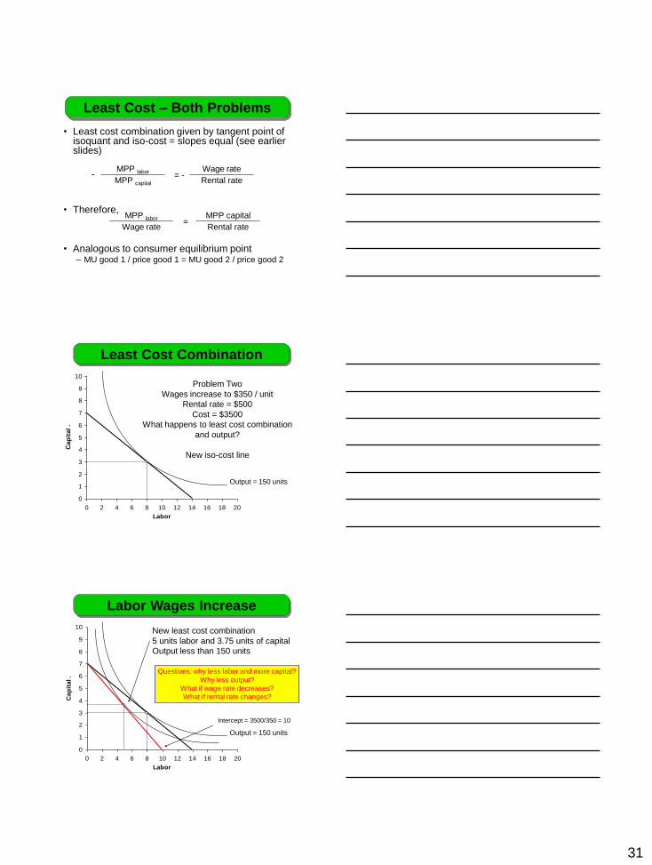
• Least cost combination given by tangent point of isoquant and iso-cost = slopes equal (see earlier slides)

-

• Therefore,

• Analogous to consumer equilibrium point

– MU good 1 / price good 1 = MU good 2 / price good 2

Least Cost – Both Problems

MPP labor

MPP capital

Wage rate

Rental rate

= -

MPP labor

Wage rate

MPP capital Rental rate

=

0

1

2

3

4

5

6

7

8

9

10

0 2 4 6 8 10 12 14 16 18 20

Labor

Ca

pit

al

.

Least Cost Combination

Problem Two

Wages increase to $350 / unit

Rental rate = $500

Cost = $3500

What happens to least cost combination

and output?

New iso-cost line

Output = 150 units

0

1

2

3

4

5

6

7

8

9

10

0 2 4 6 8 10 12 14 16 18 20

Labor

Ca

pit

al

.

Labor Wages Increase

Output = 150 units

Intercept = 3500/350 = 10

New least cost combination

5 units labor and 3.75 units of capital

Output less than 150 units

Questions: why less labor and more capital?

Why less output?

What if wage rate decreases?

What if rental rate changes?

32

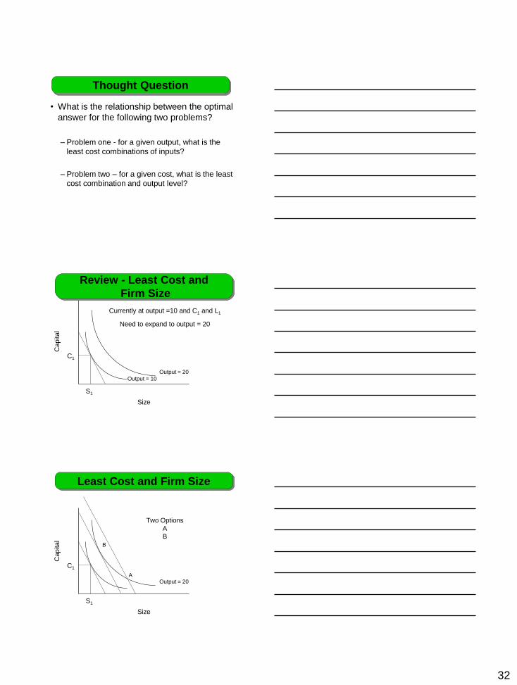
• What is the relationship between the optimal

answer for the following two problems?

– Problem one - for a given output, what is the

least cost combinations of inputs?

– Problem two – for a given cost, what is the least

cost combination and output level?

Thought Question

Size

Output = 10

Capital

C1

S1

Output = 20

Review - Least Cost and

Firm Size

Currently at output =10 and C1 and L1

Need to expand to output = 20

Least Cost and Firm Size

Size

Capital

C1

S1

Output = 20

Two Options

A

B

A

B

33

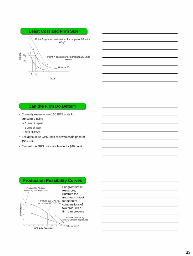
Least Cost and Firm Size

Point A costs more to produce 20 units

Why?

Size

Capital

C1

S1

Output = 20 A

B

Point B optimal combination for output of 20 units

Why?

S2

C2

• Currently manufacture 150 GPS units for

agriculture using

– 3 units of capital

– 8 units of labor

– Cost of $3500

• Sell agriculture GPS units at a wholesale price of

$50 / unit

• Can sell car GPS units wholesale for $40 / unit

Can the Firm Do Better?

0

50

100

150

200

250

300

0 20 40 60 80 100 120 140 160

GPS Units Agriculture

GP

S U

nit

s C

ars

• For given set of

resources,

illustrate the

maximum output

for different

combinations of

two products a

firm can produce

Production Possibility Curves

If produce 100 GPS Ag.

can produce 113 GPS Car

Produce 204 GPS Car

no GPS Ag. can be produced

Produce 150 GPS Ag.

no GPS Cars can be produced

Why not here?

34

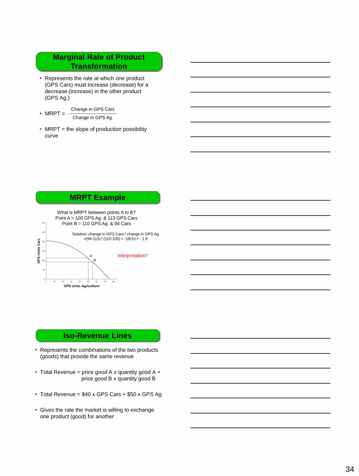
• Represents the rate at which one product

(GPS Cars) must increase (decrease) for a

decrease (increase) in the other product

(GPS Ag.)

• MRPT =

• MRPT = the slope of production possibility

curve

Marginal Rate of Product

Transformation

Change in GPS Cars

Change in GPS Ag.

0

50

100

150

200

250

300

0 20 40 60 80 100 120 140 160

GPS Units Agriculture

GP

S U

nit

s C

ars

MRPT Example

A

B

What is MRPT between points A to B?

Point A = 100 GPS Ag. & 113 GPS Cars

Point B = 110 GPS Ag. & 94 Cars

Solution: change in GPS Cars / change in GPS Ag.

=(94-113) / (110-100) = -19/10 = - 1.9

Interpretation?

• Represents the combinations of the two products

(goods) that provide the same revenue

• Total Revenue = price good A x quantity good A +

price good B x quantity good B

• Total Revenue = $40 x GPS Cars + $50 x GPS Ag

• Gives the rate the market is willing to exchange

one product (good) for another

Iso-Revenue Lines

35

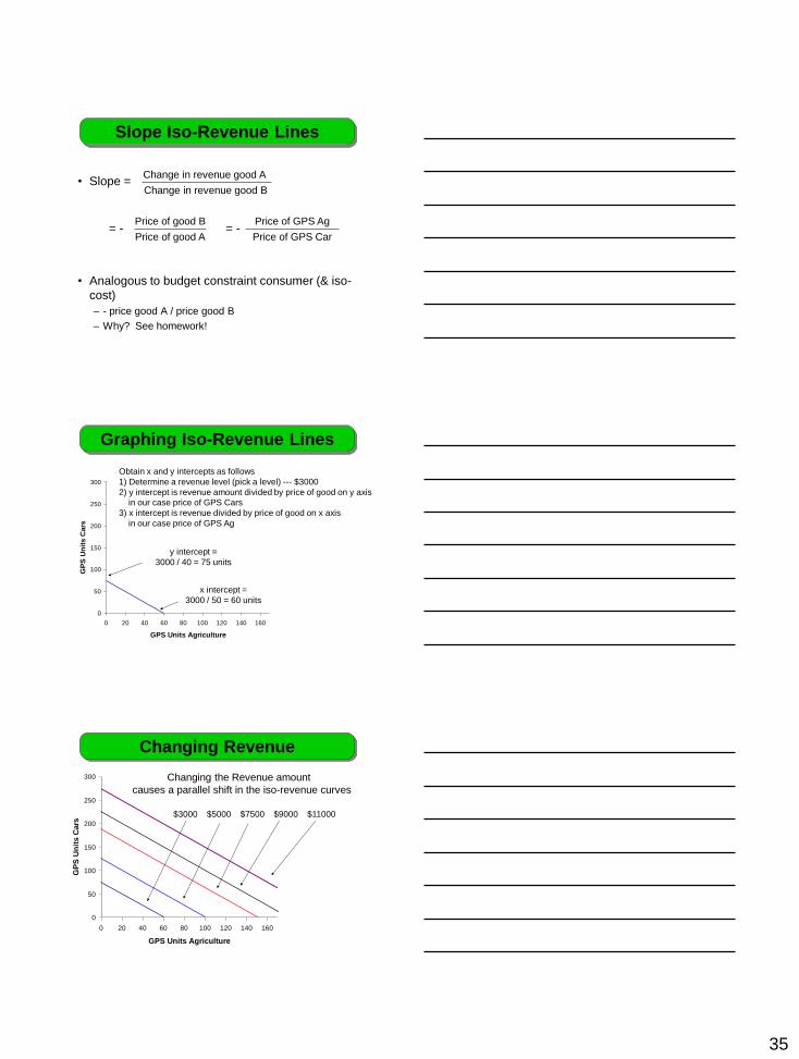
• Slope =

= - = -

• Analogous to budget constraint consumer (& iso-

cost)

– - price good A / price good B

– Why? See homework!

Slope Iso-Revenue Lines

Change in revenue good A

Change in revenue good B

Price of good B

Price of good A

Price of GPS Ag

Price of GPS Car

Graphing Iso-Revenue Lines

0

50

100

150

200

250

300

0 20 40 60 80 100 120 140 160

GPS Units Agriculture

GP

S U

nit

s C

ars

Obtain x and y intercepts as follows

1) Determine a revenue level (pick a level) --- $3000

2) y intercept is revenue amount divided by price of good on y axis

in our case price of GPS Cars

3) x intercept is revenue divided by price of good on x axis

in our case price of GPS Ag

x intercept =

3000 / 50 = 60 units

y intercept =

3000 / 40 = 75 units

Changing Revenue

0

50

100

150

200

250

300

0 20 40 60 80 100 120 140 160

GPS Units Agriculture

GP

S U

nit

s C

ars

$3000 $5000 $7500 $9000 $11000

Changing the Revenue amount

causes a parallel shift in the iso-revenue curves

36

0

50

100

150

200

250

300

0 20 40 60 80 100 120 140 160

GPS Units Agriculture

GP

S U

nit

s C

ars

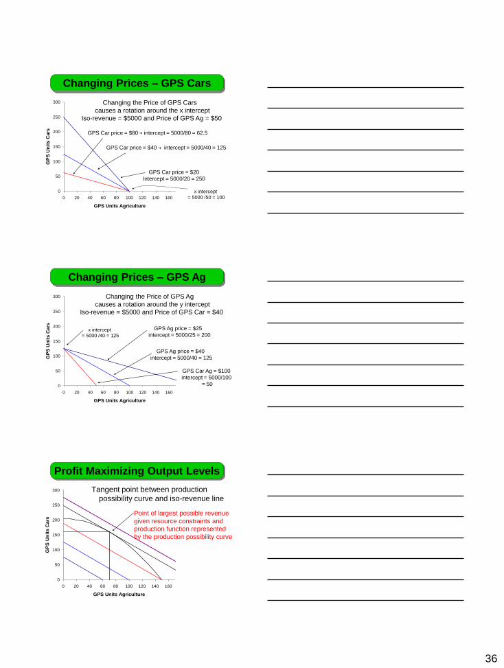
Changing Prices – GPS Cars

GPS Car price = $80 intercept = 5000/80 = 62.5

Changing the Price of GPS Cars

causes a rotation around the x intercept

Iso-revenue = $5000 and Price of GPS Ag = $50

GPS Car price = $40 intercept = 5000/40 = 125

GPS Car price = $20

Intercept = 5000/20 = 250

x intercept

= 5000 /50 = 100

0

50

100

150

200

250

300

0 20 40 60 80 100 120 140 160

GPS Units Agriculture

GP

S U

nit

s C

ars

Changing Prices – GPS Ag

GPS Ag price = $25

intercept = 5000/25 = 200

Changing the Price of GPS Ag

causes a rotation around the y intercept

Iso-revenue = $5000 and Price of GPS Car = $40

GPS Ag price = $40

intercept = 5000/40 = 125

GPS Car Ag = $100

intercept = 5000/100

= 50

x intercept

= 5000 /40 = 125

0

50

100

150

200

250

300

0 20 40 60 80 100 120 140 160

GPS Units Agriculture

GP

S U

nit

s C

ars

Tangent point between production

possibility curve and iso-revenue line

Profit Maximizing Output Levels

Point of largest possible revenue

given resource constraints and

production function represented

by the production possibility curve

37

0

50

100

150

200

250

300

0 20 40 60 80 100 120 140 160

GPS Units Agriculture

GP

S U

nit

s C

ars

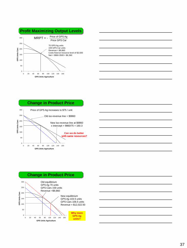
MRPT = -

Profit Maximizing Output Levels

Price of GPS Ag

Price GPS Car

70 GPS Ag units

159 GPS Car units

Revenue = $9,860

Costs fixed at resource level of $3,500

Net = 9860-3500 = $6,360

0

50

100

150

200

250

300

0 20 40 60 80 100 120 140 160

GPS Units Agriculture

GP

S U

nit

s C

ars

Change in Product Price

Old iso-revenue line = $9860

New iso-revenue line at $9860

x intercept = 9860/75 = 160.3

Price of GPS Ag increases to $75 / unit

Can we do better

with same resources?

0

50

100

150

200

250

300

0 20 40 60 80 100 120 140 160

GPS Units Agriculture

GP

S U

nit

s C

ars

Change in Product Price

Old equilibrium

GPS Ag 70 units

GPS Cars 159 units

Revenue =$9,860

New equilibrium

GPS Ag 103.5 units

GPS Cars 106.5 units

Revenue = $12,022.50

Why more

GPS Ag

units?

38

Summary #1 - Know

• Production function and related curves

– TPP, APP, and MPP

• Cost Curves

– FC, AVC, VC, AVC, TC, ATC, and MC

• Revenue Curves

– TR, AR, and MR

• Input Side - MVP

• Profit maximizing points

–MR = MC, MVP = MIC

• Short-run supply curve

–MC above AVC

• Concepts of iso-cost line and isoquants

• Marginal rate of technical substitution (MRTS)

• Least cost combination of inputs for a specific

output level

• Effects of change in input price

• Level of output and combination of inputs for

a specific budget

• Key decision rule …seek point where MRTS =

ratio of input prices, or where MPP per dollar

spent on inputs are equal.

Summary #2

• Concepts of iso-revenue line and the production possibilities frontier

• Marginal rate of product transformation (MRPT)

• Concept of profit maximizing combination of products

• Effects of change in product price

• Key decision rule – maximize profits where MRPT equals the ratio of the product prices

Summary #3