Procyclicality of US Bank Leverage

Christian Laux∗ and Thomas Rauter∗

First Version: February 19, 2014This Version: July 3, 2015

Abstract

We investigate the determinants of procyclical leverage for US commercial and savingsbanks. Understanding these determinants is important for identifying possible problemsand remedies that are as diverse as financial reporting, regulation, and bank manage-ment. We find that leverage is strongly procyclical, even after controlling for a large setof economic and bank-specific drivers of leverage. Our evidence is not consistent with thenotion that fair value accounting contributes to procyclical leverage or that historical costaccounting reduces procyclicality. Moreover, we only find a limited effect of risk-basedcapital regulation. Overall, the business model of banks seems to be more important forprocyclical bank leverage than accounting or regulation.

JEL-Classification: E32, G20, G28, G32, M41

Keywords: Procyclicality, Leverage, Banks, Fair Value Accounting, FinancialCrisis, Risk-Based Capital Regulation

∗WU (Vienna University of Economics and Business) and VGSF (Vienna Graduate School of Finance),Vienna, Austria. Corresponding author: christian.laux@wu.ac.at.

We thank Tobias Berg, Jannis Bischof, Jose Garcıa-Montalvo, Alois Geyer, Robert Kremslehner,Christian Leuz, Florian Nagler, Nikola Tarashev and seminar participants at Goethe University Frankfurt,Vienna University of Economics and Business, the 2015 European Accounting Association Meeting (Glas-gow), the 2014 European Finance Association Meeting (Lugano), the 2014 Barcelona Summer Forum,as well as the 2014 Basel Committee and Deutsche Bundesbank Joint Conference (Eltville) for helpfulcomments and suggestions.

1 Introduction

We investigate the determinants of procyclical leverage for US commercial and savings

banks to understand the role of standard setters and regulators relative to economic fac-

tors such as the business model of banks. Our findings suggest that the bank’s business

model is more important for procyclical leverage than fair value accounting or risk-based

capital regulation. Understanding the determinants of procyclical leverage is important

for identifying potential remedies that are as diverse as financial reporting, regulation, and

bank management.

The financial crisis of 2007-2009 triggered a vigorous debate about the role of fair value

accounting and revived discussions about procyclicality in banking. While the evidence

suggests that fair value accounting did not play a major role during the crisis, there is

still the concern that fair value accounting contributes to procyclical leverage.1 Procyclical

leverage arises if banks disproportionally increase debt when expanding their balance sheet

and disproportionally reduce debt when contracting total assets.2 If securities are carried

at fair value on the balance sheet, unrealized gains increase equity, which then allows a

bank to raise debt and expand. As a consequence, fair value accounting could contribute

to overheating the economy. If then a crisis hits, banks are in a worse position to deal

with distress and the disproportional reduction of debt further magnifies problems in the

financial system.

A main reference for procyclical bank leverage is the work by Adrian and Shin (2010).

1See, e.g., Benston (2008), Ryan (2008), Securities and Exchange Commission (2008), Laux and Leuz(2009), Barth and Landsman (2010), Laux and Leuz (2010), Bhat et al. (2011), Badertscher et al. (2012),and Huizinga and Laeven (2012) for the debate about the role of fair value accounting during the financialcrisis including empirical evidence. For a discussion about the significance and origin of procyclical bankleverage, see, for example, Persaud (2008), Plantin et al. (2008), International Monetary Fund (2008),Bank for International Settlements (2009), and Financial Services Authority (2009).

2We use the terms “procyclical (bank) leverage”, “leverage procyclicality”, “procyclicality”, and “pro-cyclical leverage pattern” interchangeably.

1

We adopt their definition of leverage procyclicality to allow for a direct comparison and

interpretation of results.3 The authors regress the growth rate of a bank’s book leverage on

the growth rate of its total book assets. Leverage is procyclical if the regression coefficient

is positive and significant. To identify potential determinants of procyclical bank leverage,

we extend this empirical model in several ways. First, as drivers of procyclical leverage

might vary for different types of banks, we split our sample into three subgroups: savings

banks, commercial banks with less than 20% of total assets measured at fair value (i.e.,

trading assets and AfS securities), and commercial banks with more than 20% fair value

assets. Second, we include bank-level and macroeconomic controls to see whether they can

“explain” procyclical leverage by simultaneously driving leverage growth and asset growth.

Third, we interact the growth rate of total assets with potential drivers of procyclical

leverage to identify whether these drivers magnify the link between leverage growth and

asset growth. In this context, we look at several bank and market characteristics, including

unrealized and realized gains and losses on AfS securities, realized gains and losses from

the sale of loans, trading income, and GDP growth. Finally, we investigate which types of

assets and liabilities change disproportionally when banks expand or contract their balance

sheet (that is, when total assets increase or decrease).

The focus of our analysis is on US commercial and savings banks (holding company

level) between Q3-1990 and Q1-2013. While banks in our sample hold very few trading

assets, they have a high fraction of AfS securities, which are recognized at fair value. The

variation in the types of assets that these banks hold and the differences in business models

make it particularly interesting to look at the determinants of leverage procyclicality for

these institutions.

3Regulators, the business press, and academics often refer to this study when they argue that fairvalue accounting contributes to procyclical leverage. See, for example, Financial Times (2008), Economist(2008), Beccalli et al. (2015), and Damar et al. (2013).

2

We find that leverage is strongly procyclical even after controlling for a large set of

potential determinants of bank capital structure, including macroeconomic conditions and

bank fundamentals. Despite the concern that fair value accounting could magnify pro-

cyclicality, our results are inconsistent with the notion that fair value accounting drives

procyclical leverage. In addition, we only find limited evidence that leverage procyclicality

is associated with risk-based capital regulation. Instead, procyclical leverage is related to

the bank’s business model and overall economic conditions.

First, procyclical leverage is statistically significantly higher for savings banks than for

commercial banks, including those commercial banks with more than 20% fair value assets.

Furthermore, there is no significant difference between the procyclical leverage pattern of

banks with more than 95% of total assets recognized at historical cost and banks with

more than 30% of total assets recognized at fair value. The distribution of changes in

total assets is also similar for both types of banks. As an additional test, we compare

leverage procyclicality in the period before and after the widespread introduction of fair

value accounting in the US in the mid-1990s and find that procyclical leverage was stronger

before fair value accounting was in place.

Second, the coefficient of the interaction term of unrealized gains on AfS securities with

total asset growth is insignificant for both the full sample and the different types of banks.

In contrast to unrealized gains on AfS securities, realized gains on AfS and HtM securities

do affect regulatory capital. Nevertheless, the coefficients of the corresponding interaction

terms are also insignificant. The findings for securities contrast with the findings for loans.

The interaction term of realized gains on loans is positive and significant for the full sample

as well as for savings banks and commercial banks with less than 20% fair value assets. As

loans are measured at historical cost, banks have to sell them to recognize a gain. Looking

at a subset of banks for which we can directly measure involvement in securitization,

3

we find that leverage procyclicality is stronger for those banks that are more active in

securitization.

Third, the interaction term of banks’ regulatory capital ratio is insignificant for the

whole sample and the different types of banks. One explanation might be that regula-

tory capital constraints are not binding since banks hold precautionary buffers. Another

reason might be that banks can increase their leverage without changing the regulatory

capital ratio if the average risk weight of assets decreases (Amel-Zadeh et al. (2015)). To

understand the role of regulatory risk weights, we interact changes in average risk weighted

assets with the growth in total assets and distinguish between expansions and contractions

of the balance sheet. For commercial banks with more than 20% fair value assets, we

find a negative and significant coefficient for balance sheet expansions. This is consistent

with the argument that banks which increase their balance sheet can increase leverage if

the average risk weight (of total assets) decreases. However, the coefficient is insignificant

for savings banks and commercial banks with less than 20% fair value assets. Indeed, we

find that these banks disproportionally increase loans, not securities (which generally have

lower risk weights), when expanding leverage and total assets. For commercial banks, a

procyclical reduction of leverage is strongly associated with an increase in the average risk

weight if balance sheets contract. The increase in average risk weight might force banks

to disproportionally reduce leverage if their leverage constraint is binding. However, for

both expansions and contractions of the balance sheet, the relation between changes in

average risk weighted assets and procyclical leverage might not be causal. Irrespective of

the change in regulatory risk weighted assets, banks may view liquid securities as being

less risky and therefore choose higher leverage if the fraction of liquid assets increases. In

addition, when banks reduce cash and sell liquid assets with low risk weights as a response

to an outflow of deposits, both leverage and total assets decrease while the average risk

4

weight increases.

Fourth, GDP growth is positively associated with procyclical leverage for commercial

banks. Therefore, banks do react to changes in the business environment by increasing

(decreasing) leverage and total assets. The procyclical leverage pattern of commercial

banks is also stronger if leverage is low, which is consistent with banks using an expansion

of their business to increase their leverage towards some target ratio.

We perform a range of analyses to evaluate the robustness of our findings. Overall,

we do not find any evidence supporting the claim that unrealized gains on AfS securities

contribute to procyclical leverage. The evidence on trading income is mixed and sensitive to

the inclusion of lags and the use of quarterly or yearly data. In many cases, we do not find

a significant association between the level of trading income and procyclical leverage. In

other cases, the coefficient is significant, but has sometimes a different sign than predicted.

Taken together, our results suggest that the business model and economic conditions

are more important for the procyclicality of US bank leverage than prevailing financial

reporting standards and regulatory capital requirements.

We contribute to the literature on procyclical bank leverage. Adrian and Shin (2011)

and Greenlaw et al. (2008) document a procyclical leverage pattern for US commercial

banks. These papers focus on the consequences of procyclical bank leverage on aggre-

gate liquidity, economic growth, and systemic risk. In contrast, our paper is the first

comprehensive analysis of the determinants of procyclical leverage for US commercial and

savings banks. Beccalli et al. (2015) find that the leverage procyclicality of US banks is

stronger if they are more involved in securitization. However, they do not consider the

role of accounting or capital regulation.4 Closest to our work is a contemporaneous paper

4Damar et al. (2013) find a positive effect of wholesale funding on procyclical leverage for Canadianbanks.

5

by Amel-Zadeh et al. (2015), who analyze whether regulatory risk weights and fair value

accounting contribute to the procyclical leverage of US commercial banks. They conclude

that fair value accounting does not contribute to leverage procyclicality and argue that reg-

ulation explains procyclical leverage for banks facing a binding leverage constraint while

it contributes to procyclicality for those banks that do not have a binding constraint.5

Our paper more broadly explores potential sources of procyclical bank leverage. Towards

this end, we include savings banks, study several additional determinants such as GDP

growth, and perform an asset- and liability-component analysis of procyclical leverage. We

conclude that the bank’s business model is more important for procyclical leverage than

accounting or regulation.

Xie (2015) examines whether fair value accounting increases the procyclicality of bank

lending, using approval/denial decisions on residential mortgage applications. She finds

no evidence that greater fair value accounting exposure is associated with lower (higher)

mortgage denial rates during expansionary (recessionary) periods. Her finding is consistent

with our finding that fair value accounting is not associated with procyclical leverage.

In Section 2, we develop our research questions and hypotheses. In Section 3, we present

the methodology. We describe the data in Section 4 and discuss our results in Section 5.

In Section 6, we present several robustness checks and extensions. We conclude in Section

7.

5In a previous version, Amel-Zadeh et al. (2015) argued that capital regulation explains procyclicalityfor US commercial banks since the relation between leverage growth and growth in total assets becomesinsignificant when they add the change in average risk weight as control variable to the baseline regressionmodel of Adrian and Shin (2010). In the current version, using an extended sample period, they no longerfind evidence that regulation explains procyclicality for the whole sample. Their new results, which supporta more limited role of bank regulation, are closer to our conclusion regarding the role of regulatory riskweights for procyclical leverage. Moreover, as we discuss above, it is not clear to what extent the relationbetween changes in regulatory risk weights and procyclical leverage can be interpreted as causal.

6

2 Research Questions and Hypotheses

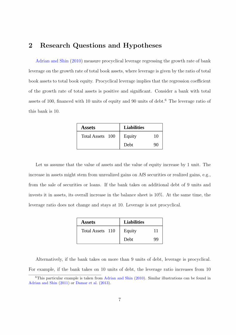
Adrian and Shin (2010) measure procyclical leverage regressing the growth rate of bank

leverage on the growth rate of total book assets, where leverage is given by the ratio of total

book assets to total book equity. Procyclical leverage implies that the regression coefficient

of the growth rate of total assets is positive and significant. Consider a bank with total

assets of 100, financed with 10 units of equity and 90 units of debt.6 The leverage ratio of

this bank is 10.

Assets Liabilities

Total Assets 100 Equity 10

Debt 90

Let us assume that the value of assets and the value of equity increase by 1 unit. The

increase in assets might stem from unrealized gains on AfS securities or realized gains, e.g.,

from the sale of securities or loans. If the bank takes on additional debt of 9 units and

invests it in assets, its overall increase in the balance sheet is 10%. At the same time, the

leverage ratio does not change and stays at 10. Leverage is not procyclical.

Assets Liabilities

Total Assets 110 Equity 11

Debt 99

Alternatively, if the bank takes on more than 9 units of debt, leverage is procyclical.

For example, if the bank takes on 10 units of debt, the leverage ratio increases from 10

6This particular example is taken from Adrian and Shin (2010). Similar illustrations can be found inAdrian and Shin (2011) or Damar et al. (2013).

7

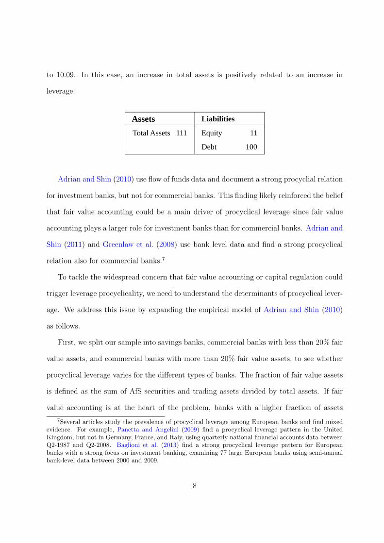
to 10.09. In this case, an increase in total assets is positively related to an increase in

leverage.

Assets Liabilities

Total Assets 111 Equity 11

Debt 100

Adrian and Shin (2010) use flow of funds data and document a strong procyclial relation

for investment banks, but not for commercial banks. This finding likely reinforced the belief

that fair value accounting could be a main driver of procyclical leverage since fair value

accounting plays a larger role for investment banks than for commercial banks. Adrian and

Shin (2011) and Greenlaw et al. (2008) use bank level data and find a strong procyclical

relation also for commercial banks.7

To tackle the widespread concern that fair value accounting or capital regulation could

trigger leverage procyclicality, we need to understand the determinants of procyclical lever-

age. We address this issue by expanding the empirical model of Adrian and Shin (2010)

as follows.

First, we split our sample into savings banks, commercial banks with less than 20% fair

value assets, and commercial banks with more than 20% fair value assets, to see whether

procyclical leverage varies for the different types of banks. The fraction of fair value assets

is defined as the sum of AfS securities and trading assets divided by total assets. If fair

value accounting is at the heart of the problem, banks with a higher fraction of assets

7Several articles study the prevalence of procyclical leverage among European banks and find mixedevidence. For example, Panetta and Angelini (2009) find a procyclical leverage pattern in the UnitedKingdom, but not in Germany, France, and Italy, using quarterly national financial accounts data betweenQ2-1987 and Q2-2008. Baglioni et al. (2013) find a strong procyclical leverage pattern for Europeanbanks with a strong focus on investment banking, examining 77 large European banks using semi-annualbank-level data between 2000 and 2009.

8

carried at fair value should exhibit stronger leverage procyclicality than banks with fewer

assets carried at fair value.

Second, we include control variables that could drive both leverage growth as well

as asset growth. If leverage and a particular control variable are positively related, the

coefficient on the control variable will be positive. In addition, if the control variable is also

positively related to asset growth, its inclusion reduces the magnitude of the coefficient on

asset growth. In this case, the control can explain (parts of) procyclical bank leverage. A

typical example is GDP growth. When the economy expands and GDP growth increases,

banks may increase both leverage and total assets. Another example is the change in

average risk weighted assets. Amel-Zadeh et al. (2015) show formally that if a bank’s

regulatory capital constraint is binding, procyclicality can only arise if the average risk

weight of assets decreases (increases) upon balance sheet expansions (contractions). We

therefore control for GDP growth and changes in average risk weighted assets. In addition,

we include unrealized gains and losses on AfS securities and net income as control variables.

We also split net income into (i) realized gains and losses on AfS and HtM securities, (ii)

gains from the sale of loans, (iii) trading income, and (iv) residual net income, which is

defined as net income minus (i), (ii), and (iii). The direct effect of these income variables

is to reduce leverage. However, if banks respond directly by raising debt, the regression

coefficient could be positive.

Third, and more importantly, we interact our key variables of interest with the change

in total assets to more directly identify the determinants of procyclical leverage. There are

several reasons for why the distinction between unrealized gains and losses on AfS securities

and the different components of net income is interesting. For example, unrealized gains

and losses on AfS securities do not affect the regulatory capital of US banks. Opponents

of fair value accounting are nevertheless concerned that its recognition could magnify pro-

9

cyclical leverage as it makes a bank look healthier and its assets more attractive. Still, the

differences in regulatory treatment might result in a difference between realized and unre-

alized gains and losses. A bank might sell AfS securities to repay debt, thereby realizing

gains from AfS securities when total assets and leverage decrease, while total unrealized

gains might result in a balance sheet expansion and an increase in leverage. Moreover,

given the focus of the discussion about procyclical leverage on securities, it is interesting

to see whether there is indeed a difference between changes in the value of securities held

as AfS and gains from the sale of loans.

A bank realizes a gain (or loss) on a loan if it decides to sell the loan to finance an

expansion of its business (e.g., increase lending) or to repay debt (reduce leverage). In

both cases, the bank’s willingness to sell the loan is higher if the realized gain from the sale

is larger. Therefore, higher gains from the sale of loans could be associated with stronger

procyclical leverage. As a result, we predict a positive coefficient on the interaction term

of realized gains on loan sales with changes in total assets.

In contrast, a bank has to report unrealized gains and losses on AfS securities as long

as these securities are held on the balance sheet and not other than temporarily impaired.

If the critics of fair value accounting are right and banks expand their balance sheet and

leverage when reporting higher unrealized gains on AfS securities, the coefficient on the

interaction term of unrealized gains on AfS securities with changes in total assets should

be positive and significant for expansions of the balance sheet. If unrealized gains are low

or even negative, a bank might be less willing to sell AfS securities. Indeed, if a US bank

holds an AfS debt security on which it reports an unrealized loss, it can avoid a negative

effect on regulatory capital by not selling the security and arguing that the impairment

is temporary. Therefore, lower unrealized gains or higher unrealized losses might reduce

procyclical leverage when total assets decrease, resulting in a positive interaction term.

10

However, opponents of fair value accounting might be concerned that the reverse is true

and that recognizing unrealized losses during a crisis might trigger a downward spiral where

banks downsize and reduce leverage. In this case, the coefficient of the interaction term

would be negative when total assets decrease.

In our robustness section, we distinguish between expansions and contractions of the

balance sheet when looking at the interaction terms of changes in total assets with unreal-

ized gains on AfS securities, realized gains on AfS and HtM securities, and trading income.

We make the same distinction for the interaction of GDP growth with changes in total

assets to account for the possibility that the coefficient has different signs for balance sheet

expansions and contractions.

To identify the role of capital regulation, we interact the level of regulatory capital

as well as the change in average risk weighted assets with the change in total assets. If

regulatory capital is high, banks are less constrained to increase leverage when they expand

such that procyclical leverage can be stronger. To capture the effect of changes in the

average risk weight, we distinguish between increases and decreases of the balance sheet.

If changes in average risk weighted assets magnify procyclical leverage, the coefficient of the

interaction term should be negative and significant upon balance sheet expansions since a

decrease in average risk weighted assets allows banks to increase leverage. In contrast, when

balance sheets contract, a positive and significant interaction term is consistent with banks

using liquid assets with low risk weights to repay debt. However, even if the coefficient of

the interaction term is significant, it is not clear to what extent the changes in regulatory

risk weights have a causal effect on procyclical leverage. Lower risk weights may go along

with lower risk and banks might increase leverage as a response to the lower risk (not the

lower risk weights). Moreover, when depositors withdraw funds, banks might use cash and

liquid assets with low risk weights to repay the depositors, which increases the average risk

11

weight and decreases total assets and leverage.

Fourth, we look at the types of assets and liabilities that are associated with procycli-

cal expansions and contractions of the balance sheet. For example, banks may expand via

securities or loans. Expansions of securities (carried at fair value) are consistent with a

decrease in the average risk weight or a lower perceived risk of these assets. In contrast,

expansions of loans are consistent with procyclical leverage being associated with the stan-

dard business model of banks and loan origination for securitization. For balance sheet

contractions it is interesting to see whether deposits, cash, and liquid assets decrease.

Fifth, we perform several additional analyses to evaluate the robustness of our findings

and to further deepen our understanding of procyclical leverage. In a first set of tests,

we investigate whether procyclical leverage is stronger for balance sheet contractions or

expansions, whether the procyclical leverage pattern prevails if we do not consider the

financial crisis, and whether procyclicality was lower before the widespread introduction of

fair value accounting in the US in the 1990s. As alternative tests of the role of fair value

accounting and the bank’s business model, we investigate the relation between procyclical

leverage and (i) the fraction of fair value assets recognized on the balance sheet (continuous

variable), (ii) the ratio of non-interest income to interest income, as well as (iii) involvement

in securitization. In a second set of robustness tests, we re-run our empirical analyses based

on yearly data and include the previous two quarters in our quarterly model to account

for the possibility that banks respond to unrealized and realized gains with some time lag.

As a final set of robustness tests, we distinguish between increases and decreases of the

balance sheet for the interactions of securities and GDP growth.

12

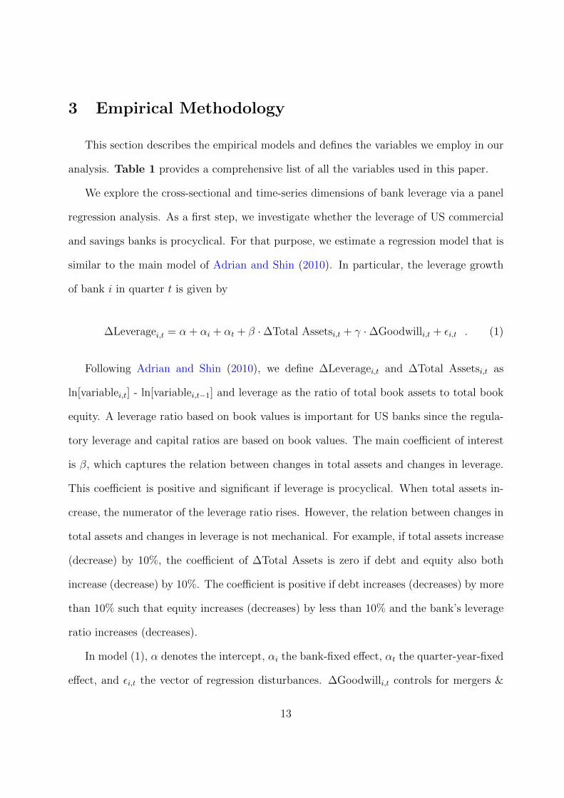
3 Empirical Methodology

This section describes the empirical models and defines the variables we employ in our

analysis. Table 1 provides a comprehensive list of all the variables used in this paper.

We explore the cross-sectional and time-series dimensions of bank leverage via a panel

regression analysis. As a first step, we investigate whether the leverage of US commercial

and savings banks is procyclical. For that purpose, we estimate a regression model that is

similar to the main model of Adrian and Shin (2010). In particular, the leverage growth

of bank i in quarter t is given by

∆Leveragei,t = α + αi + αt + β · ∆Total Assetsi,t + γ · ∆Goodwilli,t + εi,t . (1)

Following Adrian and Shin (2010), we define ∆Leveragei,t and ∆Total Assetsi,t as

ln[variablei,t] - ln[variablei,t−1] and leverage as the ratio of total book assets to total book

equity. A leverage ratio based on book values is important for US banks since the regula-

tory leverage and capital ratios are based on book values. The main coefficient of interest

is β, which captures the relation between changes in total assets and changes in leverage.

This coefficient is positive and significant if leverage is procyclical. When total assets in-

crease, the numerator of the leverage ratio rises. However, the relation between changes in

total assets and changes in leverage is not mechanical. For example, if total assets increase

(decrease) by 10%, the coefficient of ∆Total Assets is zero if debt and equity also both

increase (decrease) by 10%. The coefficient is positive if debt increases (decreases) by more

than 10% such that equity increases (decreases) by less than 10% and the bank’s leverage

ratio increases (decreases).

In model (1), α denotes the intercept, αi the bank-fixed effect, αt the quarter-year-fixed

effect, and εi,t the vector of regression disturbances. ∆Goodwilli,t controls for mergers &

13

acquisitions. It is defined as the fraction of [Goodwilli,t - Goodwilli,t−1] to [Total Assetsi,t

- Total Assetsi,t−1].8

We estimate our empirical model by ordinary least squares and adjust standard errors

for within-bank clusters (see Petersen (2009)).9 We run this regression for the whole sample

as well as separately for savings banks, commercial banks with less than 20% fair value

assets, and commercial banks with more than 20% fair value assets. The fraction of fair

value assets equals the sum of trading assets and AfS securities divided by total assets.

We extend regression model (1) by including macroeconomic conditions and bank fun-

damentals as controls since these variables might influence both ∆Leverage and ∆Total

Assets. The leverage growth of bank i in quarter t is now given by

∆Leveragei,t = α + αi + β · ∆Total Assetsi,t + γ · ∆GDPt + δ · Leveragei,t−1 (2)

+ ζ · qi,t−1 + η · Total Reg Capital Ratioi,t−1 + θ · ∆Risk Weighti,t

+ ι · Accounting Itemsi,t + κ · ∆Goodwilli,t + εi,t .

We employ ∆GDP as macroeconomic variable (defined as log difference of real GDP).

The real US GDP is an indicator of the overall economic condition in the US.10 Since

∆GDP is constant across banks within each quarter, this variable is perfectly collinear with

8Mergers & acquisitions increase total assets and, depending on the leverage ratios and the relativesize of the two banks, the book leverage of the combined bank will be larger or smaller. We do not havedata on mergers & acquisitions. Instead, we use the growth of a bank’s goodwill since the goodwill ofthe combined/surviving entity typically increases strongly after mergers & acquisitions (the residual of thepurchase price and book value of net assets is recognized as goodwill). Many small banks in our samplehave zero goodwill on their balance sheet such that ∆Goodwill based on log differences is not defined forthese banks. To overcome this problem, we use the above definition of ∆Goodwill, which is economicallyvery similar to the log definition, but has the benefit that [Total Assetsi,t - Total Assetsi,t−1] is typicallynon-zero.

9As a robustness check, we cluster standard errors at the quarter level, which slightly strengthens thestatistical significance of our results.

10We use the real GDP chained to the year 2005. As a robustness test, we use the S&P500 index andnominal GDP instead of real GDP, which does not change the nature of our results.

14

the quarter-year dummy. Therefore, we drop the quarter-year-fixed effect from regression

model (2). Leveragei,t−1 denotes the leverage ratio at the beginning of the period (lagged

leverage). qi,t−1 is the bank’s lagged market-to-book ratio of equity to control for a bank’s

growth opportunities, but also to capture possible differences between the leverage ratio

based on market and book values. We include a bank’s total regulatory capital ratio

and the change in the average risk weight, ∆Risk Weighti,t, to capture possible effects of

regulation. The total regulatory capital ratio is defined as the sum of tier 1 and tier 2

capital divided by risk-weighted assets, as specified by the Basel Committee on Banking

Supervision. The average risk weight is equal to the ratio of risk-weighted assets to total

assets and ∆Risk Weighti,t is again defined as a log difference.

In the simplest regression specification, the vector Accounting Itemsi,t contains unreal-

ized gains and losses on AfS securities as well as net income. In an extended specification,

we split up net income as discussed in Section 2. The vector then contains unrealized gains

and losses on AfS securities, realized gains and losses on AfS & HtM securities, realized

gains and losses from the sale of loans, trading income (for commercial banks), and residual

net income. We divide all accounting items by lagged total assets.

In our main empirical model, we interact potential drivers of procyclical leverage with

∆Total Assets. We estimate the following regression

15

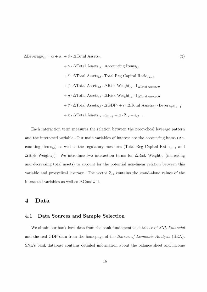
∆Leveragei,t = α + αi + β · ∆Total Assetsi,t (3)

+ γ · ∆Total Assetsi,t · Accounting Itemsi,t

+ δ · ∆Total Assetsi,t · Total Reg Capital Ratioi,t−1

+ ζ · ∆Total Assetsi,t · ∆Risk Weighti,t · 1∆Total Assets>0

+ η · ∆Total Assetsi,t · ∆Risk Weighti,t · 1∆Total Assets<0

+ θ · ∆Total Assetsi,t · ∆GDPt + ι · ∆Total Assetsi,t · Leveragei,t−1

+ κ · ∆Total Assetsi,t · qi,t−1 + µ · Zi,t + εi,t .

Each interaction term measures the relation between the procyclical leverage pattern

and the interacted variable. Our main variables of interest are the accounting items (Ac-

counting Itemsi,t) as well as the regulatory measures (Total Reg Capital Ratioi,t−1 and

∆Risk Weighti,t). We introduce two interaction terms for ∆Risk Weighti,t (increasing

and decreasing total assets) to account for the potential non-linear relation between this

variable and procyclical leverage. The vector Zi,t contains the stand-alone values of the

interacted variables as well as ∆Goodwill.

4 Data

4.1 Data Sources and Sample Selection

We obtain our bank-level data from the bank fundamentals database of SNL Financial

and the real GDP data from the homepage of the Bureau of Economic Analysis (BEA).

SNL’s bank database contains detailed information about the balance sheet and income

16

statement of all active, acquired/defunct and listed/non-listed US financial institutions

that report to the SEC, the Federal Reserve System, the FDIC or the Comptroller of the

Currency. We focus on US commercial and savings banks at the holding company level

that file Y-9C and 10-Q reports.11 Our sample covers the time period from Q3-1990 to

Q1-2013.12

We include a bank in our sample if it has non-missing and positive values for total

assets and total (book) equity. We eliminate outliers by excluding the top and bottom 1%

of observations based on the growth of total assets and the growth of leverage.13 These

selection criteria result in an initial sample of 42670 bank-quarter observations attributable

to 934 banks. Focusing our attention on banks for which all regression variables are non-

missing reduces our sample to 21620 bank-quarter observations (800 institutions).14

4.2 Descriptive Statistics

Table 2 reports averages for key characteristics of our sample banks (full sample and by

business model). The average balance sheet size is $11.34 billion. With average total assets

11All US bank holding companies are directly regulated and supervised by the Federal Reserve Systemand, if total book assets exceed $150 million ($500 million as of 2006), required to file a quarterly Y-9Creport (Consolidated Financial Statements of Holding Companies). If the holding company has more than300 shareholders, it is also required to register with the SEC and to file quarterly 10-Q and annual 10-Kreports.

12Broker-dealers that became a bank holding company during the financial crisis (e.g., Goldman Sachsand Morgan Stanley) are not included in the sample. Broker-dealers that were acquired by a commercialor savings bank are considered. For example, Merrill Lynch was a pure broker-dealer before its acquisitionby Bank of America in 2009. We do not include Merrill Lynch in our sample before 2009. However, MerrillLynch implicitly became part of our sample once it got absorbed by Bank of America. There are very fewsuch cases.

13We first cut by the growth of leverage and then by the growth of total assets. Our results do notchange qualitatively if we reverse the order or if we use different exclusion thresholds. A possible reason foroutliers are large mergers and acquisitions. By cutting the top/bottom 1% we do not eliminate the effectsof medium-sized and small mergers and acquisitions. Therefore, we control for these business combinationsby including ∆Goodwilli,t in our regression analysis. We exclude outliers for which ∆Goodwilli,t > 1 or∆Goodwilli,t < -1. Our results remain qualitatively unchanged if we do not remove these observations.

14The number of unique banks per quarter increases from 75 in Q3-1990 to 702 in Q1-2007 and stabilizesaround 700 thereafter.

17

of $1.92 billion, savings banks are smaller than commercial banks. Among commercial

banks, those with more than 20% fair value assets are significantly larger (average balance

sheet of $22.32 billion). The average leverage ratio is 11.36 and thus lower than the leverage

of large US investment banks, which is in the range of 20 to 35 (see, for example, Figure

16 in Adrian and Shin (2010)). The average savings bank has a lower leverage ratio and

a higher regulatory capital ratio than the average commercial bank. Loans are the largest

asset class and account for 65.85% of total bank assets on average. AfS securities constitute

the second largest asset class (17.60%) and HtM securities only equal 3.81% of total assets.

Trading assets play a minor role for most banks in our sample (on average 0.21% of total

assets). Deposits and senior debt are the two dominant sources of funding.

Table 3 shows summary statistics for the variables of our empirical analysis. Between

Q3-1990 and Q1-2013, the average growth of total assets and leverage of our sample banks

was 1.72% and 0.17% per quarter. Commercial banks tend to have a higher net income

and a higher market-to-book ratio of equity (qi,t−1) than savings banks. Average realized

gains on loans (0.33‰ of total assets) are higher than realized gains on AfS & HtM

securities (0.05‰), unrealized gains and losses on AfS securities (0.03‰), and trading

income (0.02‰). For savings banks, trading income is zero for 97.75% of all observations.

This lack of empirical variation makes a reliable statistical inference impossible. Therefore,

we exclude trading income in our regressions for savings banks (stand-alone and interaction

with ∆Total Assets).

18

5 Results

Figure 1 plots ∆Total Assets and ∆Leverage for all bank-quarter observations of our

sample and Figure 2 visualizes the same relation for savings and commercial banks. Each

of the graphs shows a strong procyclical leverage pattern.

In Table 4, we provide the estimation results of regression models (1) and (2) for the

full sample. The coefficient of ∆Total Assets is positive and highly statistically significant

across all regression models. When we include controls to account for macroeconomic con-

ditions and bank fundamentals, the coefficient of ∆Total Assets slightly increases. There-

fore, the procyclical leverage pattern does not seem to be heavily driven by these additional

variables.15

To quantify the economic magnitude of procyclical leverage, we look at our average

sample bank, which has total assets of $11.34 billion and a leverage ratio of 11.36. The

bank’s expected balance sheet and leverage at the end of the subsequent quarter is $11.54

billion and 11.38, respectively. The procyclical leverage coefficient of 0.758 in the full

regression model implies that a one standard-deviation increase in asset growth results in

a balance sheet of $11.94 billion and a leverage ratio of 11.69 at the end of the next quarter.

This asset growth implies an increase in the balance sheet of $408 million, which stems

from an increase of debt of $400 million and an increase of equity of $8 million. Therefore,

the marginal leverage ratio of the additional assets is 51 and more than 4 times the leverage

ratio of the bank’s initial balance sheet.

The coefficient of ∆Risk Weight is negative, which implies that an increase in the aver-

15In untabulated results, we quantify the incremental explanatory power of the bank-fixed effect and thequarter-year-fixed effect. Adding the bank-fixed effect to regression model (1) increases the adjusted R2

from 19.5% (model without any fixed effects) to 22.1%. The quarter-year-fixed effect raises the explanatorypower to 26.4%. Including both types of fixed effects results in an adjusted R2 of 28.9% as reported inTable 4 ([1]). The coefficient of ∆Total Assets is positive and highly statistically significant across allspecifications.

19

age risk weight goes along with a reduction in the leverage ratio. However, the coefficient

is only weakly significant and becomes insignificant in the full regression model.

Table 5 provides the estimation results of regression (2) by business model, splitting net

income into different components. We find strong procyclicality both for savings banks and

commercial banks. Indeed, the coefficient of ∆Total Assets is significantly higher for savings

banks than for commercial banks with more than 20% fair value assets. The difference in

coefficients is 0.144 and the p-value of the null hypothesis that this difference is zero equals

0.00%. This result arises despite the fact that savings banks hold substantially less AfS

securities and trading assets. As an alternative test, we compare the procyclical leverage

pattern of all sample banks with more than 30% fair value assets with the procyclical

leverage pattern of banks with at least 95% of total assets recognized at historical cost.

We do not find that leverage procyclicality is significantly stronger for banks that mainly

use fair value accounting (difference: 0.013; p-value: 40.52%). Importantly, the distribution

of ∆Total Assets is also similar for both types of banks. Again, this finding suggests that

fair value accounting is not a driver of procyclical bank leverage or that historical cost

accounting reduces procyclicality. Increases in unrealized gains on AfS securities and the

different components of net income directly feed into equity and thus reduce leverage,

which is reflected in the negative and statistically significant coefficients.

In Table 6, we provide the estimation results of regression model (3) for the whole

sample. The interaction term with unrealized gains and losses on AfS securities has a

negative and statistically insignificant coefficient. Therefore, higher unrealized fair value

gains on AfS securities do not magnify the procyclical leverage pattern of our sample banks.

In contrast, the coefficients of the interaction terms with net income and ∆GDP are both

positive and significant. Thus, banks’ profitability and business environment are positively

related to procyclical leverage. We also find that the procyclical leverage pattern is weaker

20

for banks with a high leverage and a high market-to-book ratio. The interaction term of

the regulatory capital ratio is insignificant. Regulatory capital constraints might not be

binding since banks hold precautionary buffers. Another reason might be that banks can

increase their leverage and balance sheet without changing the regulatory capital ratio.

The interaction term of changes in average risk weighted assets with changes in total

assets is negative and significant for balance sheet expansions. In addition, we find that a

procyclical reduction of leverage is strongly associated with an increase in the average risk

weight if balance sheets contract. The increase in average risk weight might force banks

to disproportionally reduce leverage, given a binding leverage constraint. However, it is

also possible that the coefficient captures the mechanical effect of banks reducing cash and

selling liquid assets (both have low risk weights) as a response to an outflow of deposits,

which is consistent with our findings below.

Table 7 provides the estimation results of regression (3) by business model, splitting net

income into different components. As for the full sample, the interaction term of unrealized

gains on AfS securities is insignificant for all three types of banks, again suggesting that fair

value accounting does not contribute to procyclical leverage. For savings banks, realized

gains on loans is the only variable for which the coefficient of the interaction term is

significant. The estimate is positive.

The interactions of ∆GDP, the leverage ratio, and ∆Risk Weight upon balance sheet

contractions are significant for both types of commercial banks. An interesting difference

arises with respect to the interaction of ∆Total Assets with ∆Risk Weight if total assets

increase. The coefficient is negative and highly statistically significant only for commercial

banks with more than 20% fair value assets.

To understand the drivers of procyclical leverage, it is important to investigate which

types of assets banks increase and reduce. Therefore, we take a closer look at the different

21

asset classes of our sample banks. In particular, we split ∆Total Assets from model (1)

into the quarterly growth rates of loans, AfS securities, HtM securities, and cash. Table 8

provides the estimation results for the asset-component analysis of procyclical leverage. We

distinguish between balance sheet expansions and contractions and find that for expansions

the coefficient of ∆Loans is the largest (highly significant) across all banks. This result

is not due to the fact that loans are the largest asset class on the balance sheet as the

regression coefficient captures the sensitivity of leverage to percentage changes in loans.

For balance sheet contractions, the coefficient of ∆Loans is not significant. Consequently,

banks disproportionally expand loans, not securities, when they increase leverage and total

assets. In contrast, our sample banks reduce securities and cash upon procyclical balance

sheet contractions.

In Table 9, we investigate how banks finance procyclical expansions and which types

of liabilities banks reduce upon procyclical contractions. Specifically, we replace ∆Total

Assets in model (1) with the quarterly changes of deposits, senior debt, and subordinated

debt. Leverage procyclicality is mainly associated with disproportional expansions and

contractions of deposits. Looking again separately at increases and decreases of the bal-

ance sheet, we find that for savings banks deposits are only significant when total assets

increase, not when they decrease. For commercial banks, the coefficient of ∆Deposits is

significant both for increasing and decreasing total assets. This finding is consistent with

savings banks relying more on insured deposits than commercial banks such that large,

sudden withdrawals are less likely. Unfortunately, for reasons of data availability, we can-

not differentiate between insured and uninsured deposits or interbank and non-interbank

deposits.

22

6 Robustness and Extensions

To further deepen our understanding of procyclical leverage, we extend regression model

(2) by including several additional variables that we interact with ∆Total Assets. We report

the results of this analysis in Table 10.

First, we investigate whether procyclical leverage is stronger for balance sheet contrac-

tions or expansions. In particular, we introduce a dummy variable that is equal to one if

∆Total Assets is negative and zero otherwise. The interaction term of this dummy with

∆Total Assets is positive and statistically significant, which implies that procyclicality is

stronger if banks contract their balance sheets.

Second, we analyze the impact of the recent financial crisis on procyclical leverage. We

introduce a dummy variable for the crisis period (Q3-2007 to Q4-2009), which we interact

with ∆Total Assets. The coefficient of the interaction term is negative but not statistically

significant. Therefore, leverage procyclicality was not materially different during the crisis

period and leverage remains procyclical even if we exclude the financial crisis.

Third, we compare the magnitude of procyclical leverage before and after the widespread

introduction of fair value accounting in the 1990s to test whether procyclicality increased.

We define a dummy variable, which is one for the time period Q3-1990 to Q4-1991 (pre

fair value accounting) and zero for the quarters Q1-1994 to Q1-2013 (post fair value ac-

counting). We exclude the years 1992 and 1993 from our analysis since SFAS 107 already

became effective for fiscal years ending after December 15, 1992. This accounting standard

required the disclosure of fair values for certain financial instruments and was a predecessor

of SFAS 115, which introduced the fair value recognition rules for fiscal years ending after

December 15, 1993. As a result, fiscal years 1992 and 1993 were already affected by fair

value accounting. To examine whether leverage procyclicality changed after the introduc-

23

tion of the fair value recognition rule, we interact the time dummy with ∆Total Assets.

The interaction term is positive and statistically significant.16 Therefore, the introduction

of fair value accounting did not magnify procyclical leverage. However, one needs to be

cautious not to overinterpret the results of this analysis due to potential effects associated

with the earlier introduction of SFAS 107 or other confounding events (e.g., implementation

of Basel I risk-based capital requirements in the US in Q3-1993).

Fourth, we investigate the relation between procyclical leverage and the fraction of fair

value assets recognized on a bank’s balance sheet. In line with our previous results, we

find that the interaction term of ∆Total Assets with the lagged fraction of fair value assets

is statistically insignificant.

Fifth, we use the ratio of non-interest income to interest income as an alternative

measure capturing the business model of banks. The corresponding interaction term is

positive and statistically significant. Consistent with our previous findings, the business

model is an important determinant of procyclical leverage.

Finally, we investigate the relation between procyclical leverage and off-balance sheet

guarantees provided by large commercial banks for special purpose vehicles (conduits)

through which these banks engage in securitization. Off-balance sheet guarantees are a

good proxy for a bank’s securitization activity as the amount of these guarantees increases

with the bank’s involvement in securitization. We use the data of Acharya et al. (2013),

which we retrieve from the homepage of Philipp Schnabl. The authors collect US and

European conduit-level data from rating reports by Moody’s Investor Services from Jan-

uary 2001 to December 2009. We manually match this data to our quarterly panel of US

16We estimate regression model (2) without unrealized gains on AfS securities. As this variable is onlyavailable for the post fair value accounting period, the time dummy would always take a value of onesuch that the interaction term and ∆Total Assets would be perfectly collinear. In unreported results, wealternatively define the post fair value accounting period as 1994 to 2000, 1994 to 1995, or 1994 and findthat the interaction term remains positive but becomes statistically insignificant.

24

commercial and savings banks. Only few, very large commercial banks engage in securi-

tization through special-purpose vehicles. As a result, we are able to match the data on

off-balance sheet guarantees to only 12 large commercial banks in our sample. Our fo-

cus is on liquidity guarantees since commercial banks primarily use this type of guarantee

(see, for example, Acharya et al. (2013)). The interaction term of ∆Total Assets with the

amount of off-balance sheet guarantees is positive and statistically significant for these 12

banks. Therefore, leverage procyclicality is stronger for banks that are more involved in

securitization, consistent with Beccalli et al. (2015).

We use quarterly data to investigate the leverage procyclicality of US commercial and

savings banks. For robustness, we also estimate our regressions with annual data (Table

11). Leverage remains highly procyclical. However, the coefficient of ∆Total Assets is

smaller compared to our analysis based on quarterly data (0.524 versus 0.770 for the full

sample). The interaction term of unrealized gains on AfS securities remains insignificant

for the full sample and all individual bank splits. Realized gains on AfS & HtM securities

are now positively related to procyclical leverage for commercial banks with less than 20%

fair value assets. Finally, the interaction of trading income with ∆Total Assets becomes

negative and statistically significant for commercial banks with more than 20% fair value

assets. However, these results are sensitive to whether we consider balance sheet expansions

or contractions as we discuss below.

Banks might react to both unrealized and realized gains with a time lag. To test for

this possibility, we add the previous two quarters to the corresponding accounting items of

the current quarter and re-run our empirical analyses (Table 12). The interaction terms

of unrealized gains on AfS securities and realized gains on AfS & HtM securities remain

insignificant for the full sample and subsamples. Realized gains on loan sales are no longer

significantly related to procyclical leverage for savings banks. In contrast, the interaction

25

of trading income becomes positive and statistically significant for commercial banks with

less than 20% fair value assets.

As discussed in Section 2, it might be important to distinguish between expansions and

contractions of the balance sheet for the interaction terms of securities reported at fair value

and GDP growth. We perform this analysis for our main empirical model as well as for

the versions with lagged accounting variables and yearly data (Table 13). All interaction

terms of unrealized gains on AfS securities remain insignificant with one exception. For

commercial banks with less than 20% fair value assets, the coefficient becomes marginally

significant for balance sheet expansions when including the previous two quarters. However,

the coefficient is negative, not positive. Therefore, higher unrealized gains on AfS securities

are associated with weaker, not stronger, leverage procyclicality when these banks expand

their balance sheet (controlling for the direct negative effect that unrealized gains on AfS

securities have on leverage). For the quarterly models, the interaction terms of realized

gains on AfS & HtM securities remain insignificant for the full sample and all types of

banks. However, when looking at yearly data, higher realized gains on AfS & HtM securities

are associated with stronger procyclical leverage for commercial banks. Interestingly, for

commercial banks with less than 20% fair value assets, the effect is only present for balance

sheet expansions. In contrast, for commercial banks with more than 20% fair value assets,

we find the effect only for balance sheet contractions. The latter finding is consistent with

the argument that banks are more willing to sell AfS & HtM securities to reduce leverage

when the sale of these securities results in a gain.

In our main empirical model, the interaction term of trading income becomes positive

and significant when commercial banks with less than 20% fair value assets expand their

balance sheet. This is in line with the argument that trading income might contribute to

procyclical leverage. However, for commercial banks with more than 20% fair value assets,

26

the coefficient is not significant for increasing total assets although these banks have a

much higher fraction of trading assets. Instead, the coefficient is positive and significant

for balance sheet contractions. Therefore, when these banks reduce their balance sheet,

deleveraging (procyclicality) is stronger when trading gains are higher, not when they are

lower. If we include the previous two quarters, the interaction term of trading income for

balance sheet contractions is no longer significant for commercial banks with more than

20% fair value assets. In addition, for yearly data, the interactions of trading income are

insignificant for the individual banks, but marginally significant and negative for the full

sample if total assets decrease.

Overall, we do not find any evidence supporting the claim that unrealized gains on

AfS securities contribute to procyclical leverage. The evidence on trading income is mixed

and sensitive to the inclusion of lags and the use of quarterly or yearly data. While most

people do not question the use of fair value accounting for trading assets, they might still

be concerned about its effect on procyclical leverage. Therefore, it is interesting that we

do not find a clear and strong effect of trading income on leverage procyclicality. Indeed,

in many cases we do not find a significant association between the level of trading income

and procyclical leverage. In other cases, the coefficient is significant, but has a different

sign than predicted. However, the banks in our sample only hold very little trading assets.

Moreover, those banks that do hold trading assets may do so for very different reasons

(e.g., proprietary trading, market making, and hedging) with different effects on procyclical

leverage.

Following the literature, we derive our measure of procyclicality from a regression that

relates the growth rate of a bank’s assets to the growth rate of its leverage. A positive

coefficient does not imply that leverage increases as total assets increase over time. Indeed,

as Figure 3 shows, the balance sheet of the average (equally-weighted) bank in the full

27

sample increased by a factor of nearly three between 1990 and 2013. During the same

time period, the average leverage ratio decreased from 14 to 10. This pattern also holds

individually for savings banks as well as commercial banks with more, respectively less,

than 20% of fair value assets. Therefore, procyclical bank leverage is not at odds with

banks having time-invariant target leverage ratios (Berger et al. (2008) and Gropp and

Heider (2010)).

7 Conclusion

We provide empirical evidence on the prevalence and determinants of procyclical lever-

age for US commercial and savings banks between Q3-1990 and Q1-2013. Understanding

the determinants of procyclical bank leverage is important for the identification of possible

problems and remedies that are as diverse as financial reporting, regulation, and bank

management.

Leverage is strongly procyclical for both savings and commercial banks, even after

controlling for a large set of economic and bank-specific determinants of leverage. We do

not find any evidence that fair value accounting contributes to procyclical leverage or that

historical cost accounting reduces procyclicality. Procyclical leverage is higher for savings

banks than for commercial banks, including those commercial banks with more than 20%

fair value assets. Moreover, the interaction term of unrealized gains on AfS securities with

changes in total assets is insignificant for the full sample and the different types of banks.

We find limited evidence that risk-based capital regulation systematically magnifies

procyclical leverage. The interaction term with the regulatory capital ratio is insignificant

for all regression specifications. Only for commercial banks with more than 20% fair value

assets, a reduction of the average risk weight contributes to procyclical leverage when

28

balance sheets expand. The lack of significance for the other banks is consistent with our

finding that leverage procyclicality is mainly driven by an expansion of loans (high risk

weights), not securities (low risk weights). Reductions (outflows) in deposits go along with

reductions in cash and liquid securities.

Taken together, our findings suggest that the business model and economic conditions

are more important for the procyclicality of US bank leverage than prevailing financial

reporting standards and regulatory capital requirements.

29

References

Acharya, V., Schnabl, P. and Suarez, G. (2013), ‘Securitization Without Risk Transfer’,Journal of Financial Economics 107(3), 515–536.

Adrian, T. and Shin, H. S. (2010), ‘Liquidity and Leverage’, Journal of Financial Inter-mediation 19(3), 418–437.

Adrian, T. and Shin, H. S. (2011), ‘Financial Intermediary Balance Sheet Management’,Annual Review of Financial Economics 3, 289–307.

Amel-Zadeh, A., Barth, M. E. and Landsman, W. R. (2015), ‘The Contribution of BankRegulation and Fair Value Accounting to Procyclical Leverage’, Working Paper, StanfordUniversity .

Badertscher, B. A., Burks, J. J. and Easton, P. D. (2012), ‘A Convenient Scapegoat: FairValue Accounting by Commercial Banks During the Financial Crisis’, The AccountingReview 87(1), 59–90.

Baglioni, A. S., Beccalli, E., Boitani, A. and Monticini, A. (2013), ‘Is the Leverage ofEuropean Banks Procyclical?’, Empirical Economics 45, 1251–1266.

Bank for International Settlements (2009), ‘The Role of Valuation and Leverage in Pro-cyclicality’, Committee on the Global Financial System (34).

Barth, M. E. and Landsman, W. R. (2010), ‘How Did Financial Reporting Contribute tothe Financial Crisis?’, European Accounting Review 19(3), 399–423.

Beccalli, E., Boitani, A. and Di Giuliantonio, S. (2015), ‘Leverage Pro-Cyclicality andSecuritization in US Banking’, Journal of Financial Intermediation 24(2), 200–230.

Benston, G. J. (2008), ‘The Shortcomings of Fair-Value Accounting Described in SFAS157’, Journal of Accounting and Public Policy 27(2), 101–114.

Berger, A., DeYoung, R., Flannery, M. J., Lee, D. and Oztekin, O. (2008), ‘How Do LargeBanking Organizations Manage Their Capital Ratios?’, Journal of Financial ServicesResearch 34(2), 123–149.

Bhat, G., Frankel, R. and Martin, X. (2011), ‘Panacea, Pandora’s Box, or Placebo: Feed-back in Bank Holdings of Mortgage-Backed Securities and Fair Value Accounting’, Jour-nal of Accounting and Economics 52(2-3), 153–173.

Damar, H. E., Meh, C. A. and Terajima, Y. (2013), ‘Leverage, Balance-Sheet Size andWholesale Funding’, Journal of Financial Intermediation 22(4), 639–662.

Economist (2008), ‘The Financial System: What Went Wrong’.

30

Financial Services Authority (2009), ‘The Turner Review: A Regulatory Response to theGlobal Banking Crisis’.

Financial Times (2008), ‘Insight: True Impact of Mark-to-Market on the Credit Crisis’.

Greenlaw, D., Hatzius, J., Kashyap, A. K. and Shin, H. S. (2008), ‘Leveraged Losses:Lessons from the Mortgage Market Meltdown’, US Monetary Policy Forum Report No.2 .

Gropp, R. and Heider, F. (2010), ‘The Determinants Of Bank Capital Structure’, Reviewof Finance 14(4), 587–622.

Huizinga, H. and Laeven, L. (2012), ‘Bank Valuation and Accounting Discretion During aFinancial Crisis’, Journal of Financial Economics 106(3), 614–634.

International Monetary Fund (2008), ‘Chapter 3: Fair Value Accounting and Procyclical-ity’, Global Financial Stability Report .

Laux, C. and Leuz, C. (2009), ‘The Crisis of Fair-Value Accounting: Making Sense of theRecent Debate’, Accounting, Organizations and Society 34(6-7), 826–834.

Laux, C. and Leuz, C. (2010), ‘Did Fair-Value Accounting Contribute to the FinancialCrisis?’, Journal of Economic Perspectives 24(1), 93–118.

Panetta, F. and Angelini, P. (2009), ‘Financial Sector Pro-Cyclicality: Lessons from theCrisis’, Banca D’Italia: Occasional Paper (44).

Persaud, A. (2008), ‘Regulation, Valuation and Systemic Liquidity’, Banque de France,Financial Stability Review: Special Issue on Valuation (12).

Petersen, M. A. (2009), ‘Estimating Standard Errors in Finance Panel Data Sets: Com-paring Approaches’, Review of Financial Studies 22(1), 435–480.

Plantin, G., Sapra, H. and Shin, H. S. (2008), ‘Fair Value Accounting and Financial Sta-bility’, Banque de France, Financial Stability Review: Special Issue on Valuation (12).

Ryan, S. G. (2008), ‘Accounting in and for the Subprime Crisis’, The Accounting Review83(6), 1605–1638.

Securities and Exchange Commission (2008), ‘Report and Recommendations Pursuant toSection 133 of the Emergency Economic Stabilization Act of 2008: Study on Mark-to-Market Accounting’.

Xie, B. (2015), ‘Does Fair Value Accounting Exacerbate the Procyclicality of Bank Lend-ing?’, Working Paper, Pennsylvania State University .

31

Table

sand

Fig

ure

s

Table

1:

Definit

ion

of

Regre

ssio

nV

ari

able

sT

his

tab

led

efin

esth

eva

riab

les

use

din

our

pan

elre

gre

ssio

nan

aly

sis

an

din

dic

ate

sth

eir

resp

ecti

ved

ata

sou

rce.

Vari

ab

leD

efi

nit

ion

Data

Sou

rce

Tot

alA

sset

s i,t

Book

valu

eof

all

ass

ets

reco

gn

ized

on

the

bala

nce

shee

tof

ban

ki

at

the

end

of

qu

art

ert

SN

LF

inan

cial

Lev

erag

e i,t

Tot

alA

sset

s i,t

/T

ota

lB

ook

Equ

ityi,t

SN

LF

inan

cial

GD

Pt

Rea

lU

Sgr

oss

dom

esti

cpro

du

ctat

the

end

of

qu

art

ert

BE

A

qi,t

Mar

ket

Cap

itali

zati

oni,t

/T

ota

lB

ook

Equ

ity

i,t

SN

LF

inan

cial

RW

Ai,t

Tot

alri

sk-w

eighte

dass

ets

of

ban

ki

at

the

end

of

qu

art

ert

SN

LF

inan

cial

Tot

alR

eg.

Cap

ital

Rat

ioi,t

Tot

alti

er1

and

tier

2ca

pit

al

of

ban

ki

at

the

end

of

qu

art

ert

/R

WA

i,t

SN

LF

inan

cial

Ris

kW

eigh

t i,t

Tot

alri

sk-w

eighte

dass

ets

of

ban

ki

at

the

end

of

qu

art

ert

/T

ota

lA

sset

s i,t

SN

LF

inan

cial

Good

will i,t

Exce

ssof

pu

rch

ase

pri

cep

aid

over

valu

eof

net

ass

ets

acqu

ired

of

ban

ki

at

the

end

of

qu

art

ert

SN

LF

inan

cial

∆T

otal

Ass

ets i,t

ln(T

otal

Ass

ets i,t

)-

ln(T

ota

lA

sset

s i,t−

1)

SN

LF

inan

cial

∆L

ever

age i

,tln

(Lev

erag

e i,t

)-

ln(L

ever

age i

,t−

1)

SN

LF

inan

cial

∆G

DPi,t

ln(G

DPt)

-ln

(GD

Pt−

1)

BE

A

∆R

isk

Wei

ght i,t

ln(R

isk

Wei

ght i,t

)-

ln(R

isk

Wei

ght i,t−

1)

SN

LF

inan

cial

∆G

ood

wil

l i,t

(Good

wil

l i,t

-G

ood

wil

l i,t−

1)

/(T

ota

lA

sset

s i,t

-T

ota

lA

sset

s i,t−

1)

SN

LF

inan

cial

Un

real

ized

Gai

ns

AfS

i,t

Ch

ange

inn

etu

nre

ali

zed

gain

on

AfS

secu

riti

esof

ban

ki

du

rin

gqu

art

ert

/T

ota

lA

sset

s i,t−

1S

NL

Fin

an

cial

Net

Inco

me i

,tN

etin

com

eof

ban

ki

du

rin

gqu

art

ert

/T

ota

lA

sset

s i,t−

1S

NL

Fin

an

cial

Rea

lize

dG

ain

sL

oan

s i,t

Net

gain

son

the

sale

of

loan

sof

ban

ki

du

rin

gqu

art

ert

/T

ota

lA

sset

s i,t−

1S

NL

Fin

an

cial

Rea

lize

dG

ain

sA

fS&

HtM

i,t

Net

gain

son

the

sale

of

HtM

an

dA

fSse

curi

ties

of

bank

id

uri

ng

qu

art

ert

/T

ota

lA

sset

s i,t−

1S

NL

Fin

an

cial

Tra

din

gIn

com

e i,t

Rea

lize

d&

un

reali

zed

gain

san

dlo

sses

from

trad

ing

ass

ets

of

ban

ki

du

rin

gqu

art

ert

/T

ota

lA

sset

s i,t−

1

SN

LF

inan

cial

Res

idu

alN

etIn

com

e i,t

Net

Inco

me i

,t-

Rea

lize

dG

ain

sL

oan

s i,t

-R

eali

zed

Gain

sA

fS&

HtM

i,t

-T

rad

ing

Inco

me i

,tS

NL

Fin

an

cial

32

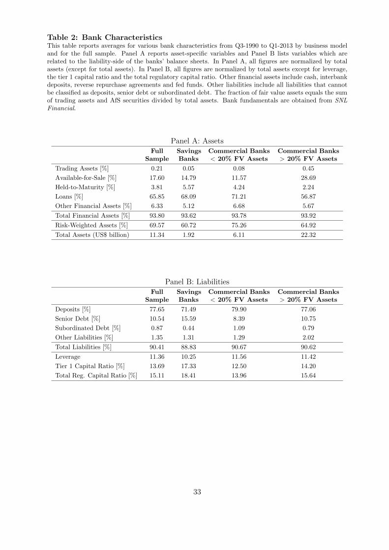
Table 2: Bank CharacteristicsThis table reports averages for various bank characteristics from Q3-1990 to Q1-2013 by business modeland for the full sample. Panel A reports asset-specific variables and Panel B lists variables which arerelated to the liability-side of the banks’ balance sheets. In Panel A, all figures are normalized by totalassets (except for total assets). In Panel B, all figures are normalized by total assets except for leverage,the tier 1 capital ratio and the total regulatory capital ratio. Other financial assets include cash, interbankdeposits, reverse repurchase agreements and fed funds. Other liabilities include all liabilities that cannotbe classified as deposits, senior debt or subordinated debt. The fraction of fair value assets equals the sumof trading assets and AfS securities divided by total assets. Bank fundamentals are obtained from SNLFinancial.

Panel A: AssetsFull

SampleSavingsBanks

Commercial Banks< 20% FV Assets

Commercial Banks> 20% FV Assets

Trading Assets [%] 0.21 0.05 0.08 0.45

Available-for-Sale [%] 17.60 14.79 11.57 28.69

Held-to-Maturity [%] 3.81 5.57 4.24 2.24

Loans [%] 65.85 68.09 71.21 56.87

Other Financial Assets [%] 6.33 5.12 6.68 5.67

Total Financial Assets [%] 93.80 93.62 93.78 93.92

Risk-Weighted Assets [%] 69.57 60.72 75.26 64.92

Total Assets (US$ billion) 11.34 1.92 6.11 22.32

Panel B: LiabilitiesFull

SampleSavingsBanks

Commercial Banks< 20% FV Assets

Commercial Banks> 20% FV Assets

Deposits [%] 77.65 71.49 79.90 77.06

Senior Debt [%] 10.54 15.59 8.39 10.75

Subordinated Debt [%] 0.87 0.44 1.09 0.79

Other Liabilities [%] 1.35 1.31 1.29 2.02

Total Liabilities [%] 90.41 88.83 90.67 90.62

Leverage 11.36 10.25 11.56 11.42

Tier 1 Capital Ratio [%] 13.69 17.33 12.50 14.20

Total Reg. Capital Ratio [%] 15.11 18.41 13.96 15.64

33

Table 3: Descriptive StatisticsThis table reports descriptive statistics for key variables of our empirical analysis. We report the 1% quantile (Q0.01), 25%quantile (Q0.25), median, mean, 75% quantile (Q0.75), 99% quantile (Q0.99), standard deviation (SD) and the number ofobservations (N). Panel A provides the statistics of the macroeconomic variables. Panels B to E list the descriptive statisticsof bank-related variables for the full sample, savings banks, commercial banks < 20% fair value assets and commercial banks> 20% fair value assets. The fraction of fair value assets equals the sum of trading assets and AfS securities divided bytotal assets. ∆GDP, ∆Leverage, ∆Total Assets, ∆Risk Weight, ∆Goodwill and the lagged total regulatory capital ratioare denoted in percent. Unrealized gains AfS, net income, realized gains loans, realized gains AfS & HtM, trading income,and residual net income are given in per mil of total assets. Total assets are denoted in US$ billion. Bank fundamentalsare obtained from SNL Financial and real GDP is retrieved from the homepage of the Bureau of Economic Analysis (USDepartment of Commerce).

Q0.01 Q0.25 Median Mean Q0.75 Q0.99 SD NPanel A: Macroeconomic Variables

∆GDP [%] -2.33 0.32 0.59 0.50 0.84 1.78 0.67 42670Panel B: Full Sample

∆Leverage [%] -16.83 -2.25 -0.07 0.17 2.45 15.40 5.10 42670∆Total Assets [%] -5.87 -0.42 1.32 1.72 3.32 14.15 3.60 42670∆Risk Weight [%] -10.22 -1.56 0.17 0.07 1.77 9.50 4.09 33421∆Goodwill [%] -7.52 0.00 0.00 0.20 0.00 13.38 5.07 38097Unrealized Gains AfS [‰] -5.10 -0.53 0.01 0.03 0.67 4.49 1.69 35638Net Income [‰] -7.56 1.35 2.25 1.92 3.00 5.49 2.38 42370Realized Gains Loans [‰] -0.06 0.00 0.05 0.33 0.27 4.72 1.16 36494Realized Gains AfS & HtM [‰] -1.51 0.00 0.00 0.05 0.06 1.68 0.90 42029Trading Income [‰] -0.05 0.00 0.00 0.02 0.00 0.56 0.22 40549Residual Net Income [‰] -9.14 0.91 1.90 1.50 2.73 5.04 2.56 34756Total Regulatory Capital Ratiot−1 [%] 9.06 12.13 13.9 15.13 16.53 35.31 5.02 38013qt−1 0.18 0.89 1.31 1.41 1.79 3.84 0.75 39331Leveraget−1 4.59 9.30 10.97 11.35 12.86 21.92 3.80 42670Total Assets [US$ billion] 0.16 0.31 0.61 11.34 1.64 167.83 102.96 42670

Panel C: Savings Banks∆Leverage [%] -13.13 -1.69 0.30 0.72 2.82 15.36 4.81 6956∆Total Assets [%] -5.81 -0.71 0.89 1.31 2.73 13.42 3.43 6956∆Risk Weight [%] -11.25 -1.42 0.33 0.26 1.93 11.41 4.09 4773∆Goodwill [%] -2.45 0.00 0.00 0.15 0.00 8.43 3.52 5644Unrealized Gains AfS [‰] -4.98 -0.35 0.00 0.01 0.44 4.14 1.77 6151Net Income [‰] -8.25 0.84 1.66 1.38 2.36 5.51 2.44 6936Realized Gains Loans [‰] -0.13 0.00 0.06 0.45 0.33 6.88 1.47 6351Realized Gains AfS & HtM [‰] -1.87 0.00 0.00 0.07 0.05 2.21 1.31 6796Residual Net Income [‰] -11.06 0.40 1.26 0.79 1.94 4.74 2.68 5690Total Regulatory Capital Ratiot−1 [%] 10.00 13.10 16.10 18.54 21.44 48.66 7.99 5335qt−1 0.20 0.78 1.06 1.17 1.44 3.50 0.62 6531Leveraget−1 3.81 7.67 9.83 10.19 12.14 21.40 4.06 6956Total Assets [US$ billion] 0.15 0.26 0.52 1.92 1.27 25.01 4.93 6956

Panel D: Commercial Banks < 20% FV Assets∆Leverage [%] -18.99 -2.14 0.00 0.18 2.45 15.50 5.20 20657∆Total Assets [%] -5.92 -0.33 1.48 1.86 3.57 13.89 3.64 20657∆Risk Weight [%] -9.57 -1.49 0.15 0.06 1.70 9.20 4.33 16448∆Goodwill [%] -7.58 0.00 0.00 0.20 0.00 13.29 5.15 18952Unrealized Gains AfS [‰] -3.01 -0.38 0.01 0.03 0.49 2.60 1.01 17687Net Income [‰] -8.56 1.33 2.29 1.88 3.06 5.59 2.60 20507Realized Gains Loans [‰] -0.07 0.00 0.06 0.36 0.30 5.34 1.29 18138Realized Gains AfS & HtM [‰] -1.47 0.00 0.00 0.02 0.02 1.38 0.60 20434Trading Income [‰] -0.02 0.00 0.00 0.02 0.00 0.39 0.23 19942Residual Net Income [‰] -10.13 0.87 1.98 1.46 2.81 5.13 2.81 17491Total Regulatory Capital Ratiot−1 [%] 8.80 11.70 13.17 13.97 15.10 28.20 3.81 18794qt−1 0.17 0.91 1.34 1.42 1.81 3.87 0.77 18948Leveraget−1 5.40 9.60 11.09 11.53 12.90 22.14 3.84 20657Total Assets [US$ billion] 0.16 0.30 0.56 6.11 1.52 106.11 41.27 20657

Panel E: Commercial Banks > 20% FV Assets∆Leverage [%] -15.73 -2.65 -0.27 -0.03 2.43 15.26 5.11 12942∆Total Assets [%] -5.74 -0.42 1.28 1.66 3.20 14.19 3.53 12942∆Risk Weight [%] -10.08 -1.66 0.16 0.04 1.83 9.28 3.71 10891∆Goodwill [%] -8.42 0.00 0.00 0.24 0.00 15.03 5.31 11986Unrealized Gains AfS [‰] -6.89 -1.05 0.08 0.06 1.33 5.96 2.38 11304Net Income [‰] -5.67 1.64 2.44 2.20 3.10 5.26 1.98 12869Realized Gains Loans [‰] -0.04 0.00 0.03 0.21 0.22 2.57 0.62 11278Realized Gains AfS & HtM [‰] -1.53 0.00 0.00 0.08 0.16 1.95 1.08 12842Trading Income [‰] -0.08 0.00 0.00 0.02 0.00 0.72 0.20 12592Residual Net Income [‰] -5.57 1.26 2.15 1.89 2.85 5.10 1.97 10978Total Regulatory Capital Ratiot−1 [%] 9.98 12.85 14.82 15.65 17.29 30.93 4.37 12182qt−1 0.20 0.97 1.40 1.50 1.90 4.03 0.78 12009Leveraget−1 5.67 9.41 11.01 11.43 12.81 21.47 3.35 12942Total Assets [US$ billion] 0.16 0.36 0.68 22.32 1.82 713.62 172.17 12942

34

Figure 1: Procyclical Leverage of US Commercial and Savings BanksThis scatter plot shows the positive and highly significant relation between ∆Total Assets and ∆Leverage(procyclical leverage) of US commercial and savings banks between Q3-1990 and Q1-2013 (42670 bank-quarter observations). ∆Total Assets and ∆Leverage are defined as ln[variablet] - ln[variablet−1] and thedata is obtained from SNL Financial.

−5% 0% 5% 10% 15%−20%

−10%

0%

10%

20%

∆Le

vera

ge

∆Total Assets

Full Sample

35

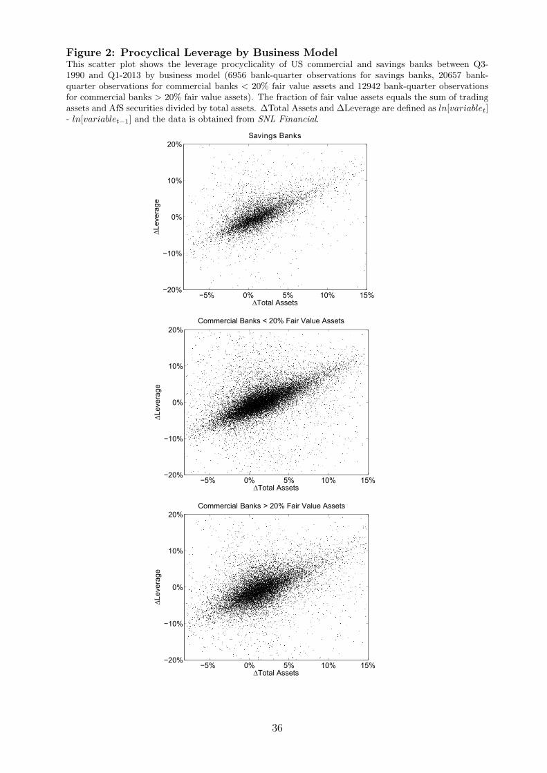
Figure 2: Procyclical Leverage by Business ModelThis scatter plot shows the leverage procyclicality of US commercial and savings banks between Q3-1990 and Q1-2013 by business model (6956 bank-quarter observations for savings banks, 20657 bank-quarter observations for commercial banks < 20% fair value assets and 12942 bank-quarter observationsfor commercial banks > 20% fair value assets). The fraction of fair value assets equals the sum of tradingassets and AfS securities divided by total assets. ∆Total Assets and ∆Leverage are defined as ln[variablet]- ln[variablet−1] and the data is obtained from SNL Financial.

−5% 0% 5% 10% 15%−20%

−10%

0%

10%

20%

∆Le

vera

ge

∆Total Assets

Savings Banks

−5% 0% 5% 10% 15%−20%

−10%

0%

10%

20%

∆Le

vera

ge

∆Total Assets

Commercial Banks < 20% Fair Value Assets

−5% 0% 5% 10% 15%−20%

−10%

0%

10%

20%

∆Le

vera

ge

∆Total Assets

Commercial Banks > 20% Fair Value Assets

36

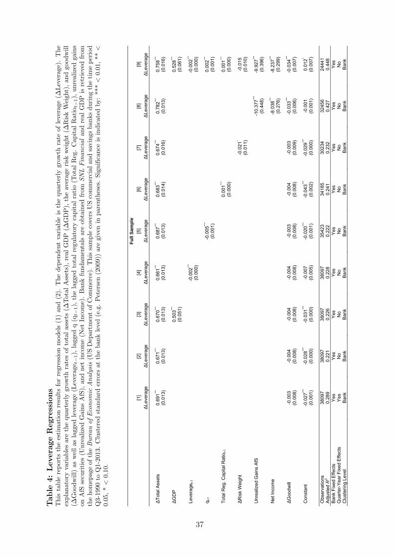
Table

4:

Levera

ge

Regre

ssio

ns

Th

ista

ble

rep

orts

the

esti

mat

ion

resu

lts

for

regr

essi

onm

od

els

(1)

an

d(2

).T

he

dep

end

ent

vari

ab

leis

the

qu

art

erly

gro

wth

rate

of

leve

rage

(∆L

ever

age)

.T

he

exp

lan

ator

yva

riab

les

are

the

qu

arte

rly

grow

thra

tes

ofto

tal

ass

ets

(∆T

ota

lA

sset

s),

real

GD

P(∆

GD

P),

the

aver

age

risk

wei

ght

(∆R

isk

Wei

ght)

,an

dgood

wil

l(∆

Good

wil

l)as

wel

las

lagg

edle

vera

ge(L

ever

age t

−1),

lagg

edq

(qt−

1),

the

lagged

tota

lre

gu

lato

ryca

pit

al

rati

o(T

ota

lR

eg.

Cap

ital

Rati

ot−

1),

un

reali

zed

gain

son

AfS

secu

riti

es(U

nre

aliz

edG

ain

sA

fS),

and

net

inco

me

(Net

Inco

me)

.B

an

kfu

nd

am

enta

lsare

ob

tain

edfr

om

SNLFinancial

an

dre

al

GD

Pis

retr

ieve

dfr

om

the

hom

epag

eof

theBureauofEconomic

Analysis

(US

Dep

art

men

tof

Com

mer

ce).

Th

issa

mp

leco

vers

US

com

mer

cial

an

dsa

vin

gs

banks

du

rin

gth

eti

me

per

iod

Q3-

1990

toQ

1-20

13.

Clu

ster

edst

andar

der

rors

atth

eb

ank

leve

l(e

.g.

Pet

erse

n(2

009))

are

giv

enin

pare

nth

eses

.Sig

nifi

can

ceis

ind

icate

dby:

***<

0.0

1,

**<

0.05

,*<

0.10

.

Fu

ll Sa

mpl

e

[1]

[2]

[3]

[4]

[5]

[6]

[7]

[8]

[9]

∆

Leve

rage

∆

Leve

rage

∆

Leve

rage

∆L

ever

age

∆Lev

erag

e ∆

Leve

rage

∆

Leve

rage

∆

Leve

rage

∆

Leve

rage

∆T

otal

Ass

ets

0.69

1***

0.67

1***

0.67

0***

0.66

1***

0.68

7***

0.68

3***

0.67

4***

0.78

2***

0.75

8***

(0

.013

) (0

.013

) (0

.013

) (0

.013

) (0

.013

) (0

.014

) (0

.016

) (0

.013

) (0

.016

)

∆G

DP

0.50

3***

0.

528**

*

(0.0

51)

(0

.061

)

Le

vera

get-1

-0.0

02**

*

-0

.002

***

(0.0

00)

(0.0

00)

q t-1

-0

.005

***

0.

002**

*

(0.0

01)

(0

.001

)

To

tal R

eg. C

apita

l Rat

iot-1

0.00

1***

0.00

1***

(0.0

00)

(0.0

00)

∆Ris

k W

eigh

t

-0

.021

*

-0.0

15

(0

.011

)

(0.0

10)

Unr

ealiz

ed G

ains

AfS

-10.

377**

* -9

.927

***

(0.4

48)

(0.3

96)

Net

Inco

me

-8

.038

***

-8.2

37**

*

(0

.276

) (0

.299

)

∆G

oodw

ill

-0.0

03

-0.0

04

-0.0

04

-0.0

04

-0.0

03

-0.0

04

-0.0

03

-0.0

33**

* -0

.034

***

(0

.008

) (0

.008

) (0

.008

) (0

.008

) (0

.008

) (0

.008

) (0

.009

) (0

.006

) (0

.007

)

C

onst

ant

-0.0

27**

* -0

.028

***

-0.0

31**

* -0

.007

-0

.020

***

-0.0

43**

* -0

.029

***

-0.0

01

0.01

2*

(0.0

01)

(0.0

00)

(0.0

00)

(0.0

05)

(0.0

01)

(0.0

02)

(0.0

00)

(0.0

01)

(0.0

07)

Obs

erva

tions

38

097

3809

7 38

097

3809

7 35

423

3418

5 30

234

3245

6 24

441

Adju

sted

R2

0.28

9 0.

221

0.22

6 0.

228

0.22

2 0.

241

0.23

2 0.

427

0.44

8 Ba

nk F

ixed

Effe

cts

Yes

Yes

Yes

Yes

Yes

Yes

Yes

Yes

Yes

Qua

rter-Y

ear F

ixed

Effe

cts

Yes

No

No

No

No

No

No

No

No

Clu

ster

ing

Leve

l B

ank

Ban

k B

ank

Bank

B

ank

Ban

k B

ank

Ban

k B

ank

37

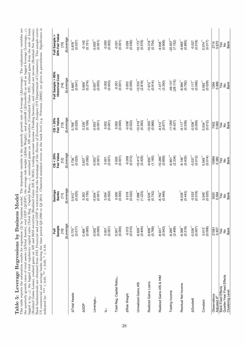
Table

5:

Levera

ge

Regre

ssio

ns

by

Busi

ness

Model

Th

ista

ble

rep

ort

sth

ees

tim

ati

on

resu

lts

for

regre

ssio

n(2

)by

bu

sin

ess

mod

el.

Th

ed

epen

den

tvari

ab

leis

the

qu

art

erly

gro

wth

rate

of

lever

age

(∆L

ever

age)

.T

he

exp

lan

ato

ryvari

ab

les

are

the

qu

art

erly

gro

wth

rate

sof

tota

lass

ets

(∆T

ota

lA

sset

s),

real

GD

P(∆

GD

P),

the

aver

age

risk

wei

ght

(∆R

isk

Wei

ght)

,an

dgood

will

(∆G

ood

will)

as

wel

las

lagged

lever

age

(Lev

erage t

−1),

lagged

q(q

t−1),

the

lagged

tota

lre

gu

lato

ryca

pit

al

rati

o(T

ota

lR

eg.

Cap

ital

Rati

ot−

1),

un

realize

dgain

son

AfS

secu

riti

es(U

nre

alize

dG

ain

sA

fS),

reali

zed

gain

sfr

om

the

sale

of

loan

s(R

ealize

dG

ain

sL

oan

s),

realize

dgain

son

AfS

an

dH

tMse

curi

ties

(Rea

lize

dG

ain

sA

fS&

HtM

),tr

ad

ing

acc

ou

nt

inco

me

(Tra

din

gIn

com

e),

an

dre

sid

ual

net

inco

me

(Res

idu

al

Net

Inco

me)

.B

an

kfu

nd

am

enta

lsare

ob

tain

edfr

om

SNL

Financial

an

dre

al

GD

Pis

retr

ieved

from

the

hom

epage

of

theBureauofEconomic

Analysis

(US

Dep

art

men

tof

Com

mer

ce).

Th

issa

mp

leco

ver

sU

Sco

mm

erci

al

an

dsa

vin

gs

ban

ks

du

rin

gth

eti

me

per

iod

Q3-1

990

toQ

1-2

013.

Clu

ster

edst

an

dard

erro

rsat

the

ban

kle

vel

(e.g

.P

eter

sen

(2009))

are

giv

enin

pare

nth

eses

.S

ign

ifica

nce

isin

dic

ate

dby:

***<

0.0

1,

**<

0.0

5,

*<

0.1

0.

Fu

ll

Sam

ple

Savi

ngs

Ban

ks

CB

< 2

0%

Fair

Valu

e C

B >

20%

Fa

ir Va

lue

Full

Sam

ple

> 95

%

His

toric

al C

ost

Full

Sam

ple

> 30

% F

air V

alue

[10]

[1

1]

[12]

[1

3]

[14]

[1

5]

∆

Leve

rage

∆L

ever

age

∆Le

vera

ge

∆Lev

erag

e ∆

Leve

rage

∆

Leve

rage

∆To

tal A

sset

s 0.

770**

* 0.

912**

* 0.

736**

* 0.

768**

* 0.

865**

* 0.

878**

*

(0.0

17)

(0.0

25)

(0.0

25)

(0.0

29)

(0.0

41)

(0.0

37)

∆

GD

P 0.

484**

* 0.

263*

0.63

7***

0.23

9**

0.66

9**

-0.1

45

(0

.065

) (0

.150

) (0

.092

) (0

.109

) (0

.274

) (0

.151

)

Leve

rage

t-1

-0.0

02**

* -0

.004

***

-0.0

03**

* -0

.003

***

-0.0

07**

* -0

.005

***

(0

.000

) (0

.001

) (0

.001

) (0

.001

) (0

.003

) (0

.001

)

q t-1

0.

001*

0.00

4* 0.

001

0.00

2 -0

.002

-0

.000

(0.0

01)

(0.0

02)

(0.0

01)

(0.0

01)

(0.0

03)

(0.0

02)

To

tal R

eg. C

apita

l Rat

iot-1

0.

001**

0.

000

0.00

0 0.

000

-0.0

01

-0.0

01

(0

.000

) (0

.000

) (0

.001

) (0

.000

) (0

.001

) (0

.001

)

∆R

isk

Wei

ght

-0.0

12

0.01

9 -0

.009

-0

.036

* 0.

003

0.02

6

(0.0

10)

(0.0

22)

(0.0

12)

(0.0

22)

(0.0

05)

(0.0

36)

U

nrea

lized

Gai

ns A

fS

-9.9

29**

* -7

.088

***

-10.

413**

* -1

0.51

8***

-12.

533**

* -1

0.17

2***

(0

.444

) (1

.223

) (0

.425

) (0

.393

) (2

.819

) (0

.579

)

Rea

lized

Gai

ns L

oans

-9

.858

***

-9.5

35**

* -9

.650

***

-10.

555**

* -7

.972

***

-10.

318**

*

(0.7

68)

(0.7

42)

(1.1

65)

(0.9

66)

(0.9

14)

(0.7

04)

R

ealiz

ed G

ains

AfS

& H

tM

-8.9

31**

* -8

.762

***

-10.

280**

* -8

.512

***

-7.4

77**

-9.9

36**

*

(0.5

43)

(0.9

49)

(0.8

59)

(0.6

77)

(3.3

50)

(0.9

08)

Tr

adin

g In

com

e -8

.265

***

-6

.901

***

-11.

055*

-49.

131*

-20.

007**

*

(2.4

06)

(2

.334

) (6

.427

) (2

8.11

5)

(7.1

52)

R

esid

ual N

et In

com

e -8

.368

***

-8.0

39**

* -8

.146

***

-9.1

17**

* -8

.564

***

-9.6

65**

*

(0.3

19)

(0.4

43)

(0.4

35)

(0.5

38)

(0.7

92)

(0.8

65)

∆

Goo

dwill

-0

.036

***

-0.0

33*

-0.0

37**

* -0

.036

***

-0.1

17**

-0.0

27

(0

.007

) (0

.019

) (0

.012

) (0

.009

) (0

.056

) (0

.018

)

Con

stan

t 0.

013*

0.04

5* 0.

049**

* 0.

034**

* 0.

092**

* 0.

074**

*

(0.0

08)

(0.0

25)

(0.0

14)

(0.0

12)

(0.0

29)

(0.0

17)

Obs

erva

tions

21

581

3020

10

984

7402

12

64

2714

A

djus

ted

R2

0.45

7 0.

594

0.38

0 0.

560

0.48

6 0.

670

Ban

k Fi

xed

Effe

cts

Yes

Yes

Yes

Yes

Yes

Yes

Qua

rter-Y

ear F

ixed

Effe

cts

No

No

No

No

No

No

Clu

ster

ing

Leve

l Ba

nk

Ban

k Ba

nk

Ban

k B

ank

Bank

38

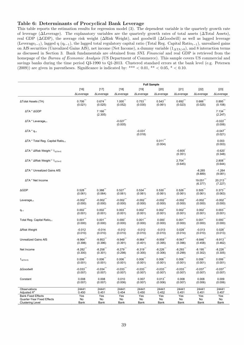
Table 6: Determinants of Procyclical Bank LeverageThis table reports the estimation results for regression model (3). The dependent variable is the quarterly growth rateof leverage (∆Leverage). The explanatory variables are the quarterly growth rates of total assets (∆Total Assets),real GDP (∆GDP), the average risk weight (∆Risk Weight), and goodwill (∆Goodwill) as well as lagged leverage(Leveraget−1), lagged q (qt−1), the lagged total regulatory capital ratio (Total Reg. Capital Ratiot−1), unrealized gainson AfS securities (Unrealized Gains AfS), net income (Net Income), a dummy variable (1∆TA>0), and 8 interaction termsas discussed in Section 3. Bank fundamentals are obtained from SNL Financial and real GDP is retrieved from thehomepage of the Bureau of Economic Analysis (US Department of Commerce). This sample covers US commercial andsavings banks during the time period Q3-1990 to Q1-2013. Clustered standard errors at the bank level (e.g. Petersen(2009)) are given in parentheses. Significance is indicated by: *** < 0.01, ** < 0.05, * < 0.10.

Full Sample

[16] [17] [18] [19] [20] [21] [22] [23]

∆Leverage ∆Leverage ∆Leverage ∆Leverage ∆Leverage ∆Leverage ∆Leverage ∆Leverage

∆Total Assets (TA) 0.706*** 0.674*** 1.000*** 0.753*** 0.543*** 0.692*** 0.666*** 0.895*** (0.021) (0.025) (0.052) (0.030) (0.061) (0.023) (0.025) (0.108) ∆TA * ∆GDP 7.166*** 7.134*** (2.305) (2.247) ∆TA * Leveraget-1 -0.027*** -0.022*** (0.005) (0.006) ∆TA * qt-1 -0.031* -0.047** (0.018) (0.021) ∆TA * Total Reg. Capital Ratiot-1 0.011*** 0.003 (0.004) (0.003) ∆TA * ∆Risk Weight * 1(∆TA>0) -0.605* -0.620* (0.351) (0.348) ∆TA * ∆Risk Weight * 1(∆TA<0) 2.704*** 2.808*** (0.645) (0.644) ∆TA * Unrealized Gains AfS -8.265 -1.264 (8.889) (9.081) ∆TA * Net Income 19.051*** 20.213*** (6.377) (7.227) ∆GDP 0.528*** 0.388*** 0.527*** 0.534*** 0.530*** 0.526*** 0.505*** 0.373*** (0.061) (0.064) (0.061) (0.061) (0.061) (0.061) (0.061) (0.063) Leveraget-1 -0.002*** -0.002*** -0.002*** -0.002*** -0.002*** -0.002*** -0.002*** -0.002*** (0.000) (0.000) (0.000) (0.000) (0.000) (0.000) (0.000) (0.000) qt-1 0.002*** 0.002*** 0.003*** 0.002*** 0.002*** 0.002*** 0.002** 0.003*** (0.001) (0.001) (0.001) (0.001) (0.001) (0.001) (0.001) (0.001) Total Reg. Capital Ratiot-1 0.001*** 0.001*** 0.000** 0.001*** 0.000* 0.001*** 0.001*** 0.000*** (0.000) (0.000) (0.000) (0.000) (0.000) (0.000) (0.000) (0.000) ∆Risk Weight -0.012 -0.014 -0.012 -0.012 -0.013 0.028** -0.013 0.028** (0.010) (0.010) (0.010) (0.010) (0.010) (0.014) (0.010) (0.013) Unrealized Gains AfS -9.964*** -9.953*** -9.949*** -9.964*** -9.959*** -9.947*** -9.846*** -9.913*** (0.398) (0.396) (0.391) (0.401) (0.395) (0.396) (0.458) (0.462) Net Income -8.282*** -8.258*** -8.279*** -8.319*** -8.226*** -8.293*** -8.195*** -8.226*** (0.300) (0.301) (0.298) (0.300) (0.306) (0.299) (0.302) (0.305) 1(∆TA>0) 0.006*** 0.006*** 0.006*** 0.006*** 0.006*** 0.006*** 0.006*** 0.006*** (0.001) (0.001) (0.001) (0.001) (0.001) (0.001) (0.001) (0.001) ∆Goodwill -0.033*** -0.034*** -0.033*** -0.033*** -0.033*** -0.033*** -0.037*** -0.037*** (0.007) (0.007) (0.007) (0.007) (0.007) (0.007) (0.007) (0.007) Constant 0.008 0.008 0.010 0.007 0.013** 0.008 0.008 0.009 (0.007) (0.007) (0.006) (0.007) (0.006) (0.007) (0.006) (0.006) Observations 24441 24441 24441 24441 24441 24441 24441 24441 Adjusted R2 0.450 0.451 0.454 0.450 0.452 0.451 0.451 0.457 Bank Fixed Effects Yes Yes Yes Yes Yes Yes Yes Yes Quarter-Year Fixed Effects No No No No No No No No Clustering Level Bank Bank Bank Bank Bank Bank Bank Bank

39

Table 7: Determinants of Procyclical Bank Leverage by Business ModelThis table reports the estimation results for regression (3) by business model. The dependent variable is the quarterly growthrate of leverage (∆Leverage). The explanatory variables are the quarterly growth rates of total assets (∆Total Assets), realGDP (∆GDP), the average risk weight (∆Risk Weight), and goodwill (∆Goodwill) as well as lagged leverage (Leveraget−1),lagged q (qt−1), the lagged total regulatory capital ratio (Total Reg. Capital Ratiot−1), unrealized gains on AfS securities(Unrealized Gains AfS), realized gains from the sale of loans (Realized Gains Loans), realized gains on AfS and HtM securities(Realized Gains AfS & HtM), trading account income (Trading Income), residual net income (Residual Net Income), a dummyvariable (1∆TA>0), and 11 interaction terms as discussed in Section 3. Bank fundamentals are obtained from SNL Financialand real GDP is retrieved from the homepage of the Bureau of Economic Analysis (US Department of Commerce). Thissample covers US commercial and savings banks during the time period Q3-1990 to Q1-2013. Clustered standard errors atthe bank level (e.g. Petersen (2009)) are given in parentheses. Significance is indicated by: *** < 0.01, ** < 0.05, * < 0.10.

Full Sample Savings Banks CB < 20% FV CB > 20% FV [24] [25] [26] [27] ∆Leverage ∆Leverage ∆Leverage ∆Leverage ∆Total Assets (TA) 0.945*** 0.702*** 0.885*** 0.897*** (0.110) (0.212) (0.143) (0.175) ∆TA * ∆GDP 7.525*** -0.861 9.126** 8.232* (2.509) (5.665) (3.606) (4.263) ∆TA * Leveraget-1 -0.025*** 0.000 -0.021*** -0.020** (0.006) (0.016) (0.008) (0.009) ∆TA * qt-1 -0.044* 0.032 -0.052 -0.067** (0.024) (0.039) (0.032) (0.033) ∆TA * Total Reg. Capital Ratiot-1 0.001 0.006 -0.000 0.003 (0.003) (0.006) (0.004) (0.005) ∆TA * ∆Risk Weight * 1(∆TA>0) -0.629* -0.057 -0.385 -1.562*** (0.354) (0.680) (0.352) (0.596) ∆TA * ∆Risk Weight * 1(∆TA<0) 2.999*** 0.566 3.071** 3.588*** (0.707) (1.199) (1.192) (1.066) ∆TA * Unrealized Gains AfS -2.565 -17.885 -16.707 4.652 (9.866) (15.885) (20.177) (12.281) ∆TA * Realized Gains Loans 31.923*** 47.574** 33.522*** 22.579 (8.258) (19.124) (9.698) (34.141) ∆TA * Realized Gains AfS & HtM 21.713 -5.121 10.850 25.472 (18.772) (15.088) (20.589) (32.937) ∆TA * Trading Income 65.055 55.907 274.931 (67.526) (50.961) (178.065) ∆TA * Residual Net Income 19.645** 14.003 22.556** 13.147 (7.796) (11.439) (9.742) (14.054) ∆GDP 0.326*** 0.243 0.435*** 0.075 (0.067) (0.165) (0.098) (0.105) Leveraget-1 -0.002*** -0.004*** -0.003*** -0.003*** (0.000) (0.001) (0.001) (0.001) qt-1 0.002*** 0.004 0.002* 0.004*** (0.001) (0.003) (0.001) (0.001) Total Reg. Capital Ratiot-1 0.000** 0.000 0.001 -0.000 (0.000) (0.000) (0.000) (0.000) ∆Risk Weight 0.032** 0.024 0.024 0.039 (0.014) (0.033) (0.017) (0.030) Unrealized Gains AfS -9.906*** -7.069*** -10.139*** -10.573*** (0.510) (1.089) (0.426) (0.505) Realized Gains Loans -10.294*** -9.837*** -10.080*** -11.128*** (0.655) (0.860) (1.033) (0.964) Realized Gains AfS & HtM -8.832*** -8.495*** -9.835*** -8.682*** (0.515) (0.938) (0.854) (0.654) Trading Income -9.061*** -7.194*** -17.614** (2.558) (2.215) (7.004) Residual Net Income -8.306*** -7.804*** -8.045*** -9.258*** (0.325) (0.451) (0.445) (0.573) 1(∆TA>0) 0.006*** 0.001 0.007*** 0.006*** (0.001) (0.002) (0.001) (0.002) ∆Goodwill -0.038*** -0.040** -0.039*** -0.033*** (0.007) (0.017) (0.012) (0.009) Constant 0.011 0.048** 0.041*** 0.033*** (0.007) (0.024) (0.012) (0.012) Observations 21581 3020 10984 7402 Adjusted R2 0.465 0.596 0.390 0.567 Bank Fixed Effects Yes Yes Yes Yes Quarter-Year Fixed Effects No No No No Clustering Level Bank Bank Bank Bank

40

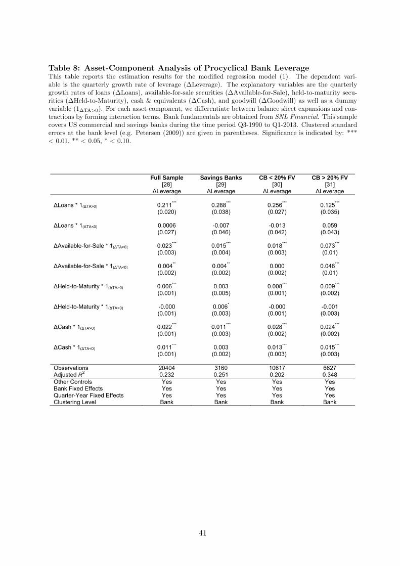
Table 8: Asset-Component Analysis of Procyclical Bank LeverageThis table reports the estimation results for the modified regression model (1). The dependent vari-able is the quarterly growth rate of leverage (∆Leverage). The explanatory variables are the quarterlygrowth rates of loans (∆Loans), available-for-sale securities (∆Available-for-Sale), held-to-maturity secu-rities (∆Held-to-Maturity), cash & equivalents (∆Cash), and goodwill (∆Goodwill) as well as a dummyvariable (1∆TA>0). For each asset component, we differentiate between balance sheet expansions and con-tractions by forming interaction terms. Bank fundamentals are obtained from SNL Financial. This samplecovers US commercial and savings banks during the time period Q3-1990 to Q1-2013. Clustered standarderrors at the bank level (e.g. Petersen (2009)) are given in parentheses. Significance is indicated by: ***< 0.01, ** < 0.05, * < 0.10.

Full Sample Savings Banks CB < 20% FV CB > 20% FV [28] [29] [30] [31] ∆Leverage ∆Leverage ∆Leverage ∆Leverage ∆Loans * 1(∆TA>0) 0.211*** 0.288*** 0.256*** 0.125*** (0.020) (0.038) (0.027) (0.035) ∆Loans * 1(∆TA<0) 0.0006 -0.007 -0.013 0.059 (0.027) (0.046) (0.042) (0.043) ∆Available-for-Sale * 1(∆TA>0) 0.023*** 0.015*** 0.018*** 0.073*** (0.003) (0.004) (0.003) (0.01) ∆Available-for-Sale * 1(∆TA<0) 0.004** 0.004** 0.000 0.046*** (0.002) (0.002) (0.002) (0.01) ∆Held-to-Maturity * 1(∆TA>0) 0.006*** 0.003 0.008*** 0.009*** (0.001) (0.005) (0.001) (0.002) ∆Held-to-Maturity * 1(∆TA<0) -0.000 0.006* -0.000 -0.001 (0.001) (0.003) (0.001) (0.003) ∆Cash * 1(∆TA>0) 0.022*** 0.011*** 0.028*** 0.024*** (0.001) (0.003) (0.002) (0.002) ∆Cash * 1(∆TA<0) 0.011*** 0.003 0.013*** 0.015*** (0.001) (0.002) (0.003) (0.003) Observations 20404 3160 10617 6627 Adjusted R2 0.232 0.251 0.202 0.348 Other Controls Yes Yes Yes Yes Bank Fixed Effects Yes Yes Yes Yes Quarter-Year Fixed Effects Yes Yes Yes Yes Clustering Level Bank Bank Bank Bank

41

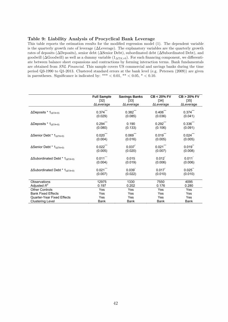
Table 9: Liability Analysis of Procyclical Bank LeverageThis table reports the estimation results for the modified regression model (1). The dependent variableis the quarterly growth rate of leverage (∆Leverage). The explanatory variables are the quarterly growthrates of deposits (∆Deposits), senior debt (∆Senior Debt), subordinated debt (∆Subordinated Debt), andgoodwill (∆Goodwill) as well as a dummy variable (1∆TA>0). For each financing component, we differenti-ate between balance sheet expansions and contractions by forming interaction terms. Bank fundamentalsare obtained from SNL Financial. This sample covers US commercial and savings banks during the timeperiod Q3-1990 to Q1-2013. Clustered standard errors at the bank level (e.g. Petersen (2009)) are givenin parentheses. Significance is indicated by: *** < 0.01, ** < 0.05, * < 0.10.

Full Sample Savings Banks CB < 20% FV CB > 20% FV [32] [33] [34] [35] ∆Leverage ∆Leverage ∆Leverage ∆Leverage ∆Deposits * 1(∆TA>0) 0.374*** 0.382*** 0.406*** 0.374*** (0.029) (0.085) (0.036) (0.041) ∆Deposits * 1(∆TA<0) 0.294*** 0.190 0.292*** 0.336*** (0.080) (0.133) (0.106) (0.091) ∆Senior Debt * 1(∆TA>0) 0.020*** 0.069*** 0.019*** 0.024*** (0.004) (0.016) (0.005) (0.005) ∆Senior Debt * 1(∆TA<0) 0.022*** 0.037* 0.021*** 0.019** (0.005) (0.020) (0.007) (0.008) ∆Subordinated Debt * 1(∆TA>0) 0.011*** 0.015 0.012* 0.011* (0.004) (0.019) (0.006) (0.006) ∆Subordinated Debt * 1(∆TA<0) 0.021*** 0.039* 0.017* 0.025** (0.007) (0.022) (0.010) (0.010) Observations 12975 1330 7550 4095 Adjusted R2 0.197 0.202 0.176 0.280 Other Controls Yes Yes Yes Yes Bank Fixed Effects Yes Yes Yes Yes Quarter-Year Fixed Effects Yes Yes Yes Yes Clustering Level Bank Bank Bank Bank

42

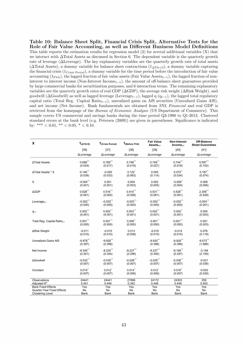
Table 10: Balance Sheet Split, Financial Crisis Split, Alternative Tests for theRole of Fair Value Accounting, as well as Different Business Model DefinitionsThis table reports the estimation results for regression model (2) for several additional variables (X) thatwe interact with ∆Total Assets as discussed in Section 6. The dependent variable is the quarterly growthrate of leverage (∆Leverage). The key explanatory variables are the quarterly growth rate of total assets(∆Total Assets), a dummy variable for balance sheet contractions (1∆TA<0), a dummy variable capturingthe financial crisis (1Crisis Period), a dummy variable for the time period before the introduction of fair valueaccounting (1FVA), the lagged fraction of fair value assets (Fair Value Assetst−1), the lagged fraction of non-interest to interest income (Non-Interest Incomet−1), the amount of off-balance sheet guarantees providedby large commercial banks for securitization purposes, and 6 interaction terms. The remaining explanatoryvariables are the quarterly growth rates of real GDP (∆GDP), the average risk weight (∆Risk Weight), andgoodwill (∆Goodwill) as well as lagged leverage (Leveraget−1), lagged q (qt−1), the lagged total regulatorycapital ratio (Total Reg. Capital Ratiot−1), unrealized gains on AfS securities (Unrealized Gains AfS),and net income (Net Income). Bank fundamentals are obtained from SNL Financial and real GDP isretrieved from the homepage of the Bureau of Economic Analysis (US Department of Commerce). Thissample covers US commercial and savings banks during the time period Q3-1990 to Q1-2013. Clusteredstandard errors at the bank level (e.g. Petersen (2009)) are given in parentheses. Significance is indicatedby: *** < 0.01, ** < 0.05, * < 0.10.

X 1(∆TA<0) 1(Crisis Period) 1(Before FVA) Fair Value Assetst-1

Non-Interest Incomet-1

Off-Balance Sheet Guarantees

[36] [37] [38] [39] [40] [41]

∆Leverage ∆Leverage ∆Leverage ∆Leverage ∆Leverage ∆Leverage

∆Total Assets 0.688*** 0.769*** 0.746*** 0.748*** 0.744*** 0.597*** (0.024) (0.017) (0.016) (0.027) (0.019) (0.102)

∆Total Assets * X 0.146*** -0.055 0.122* 0.055 0.070** 0.167** (0.039) (0.033) (0.063) (0.114) (0.034) (0.074)

X -0.004*** 0.001 0.004 0.002 -0.009** 0.008(0.001) (0.001) (0.003) (0.005) (0.004) (0.006)

∆GDP 0.528*** 0.516*** 0.914*** 0.531*** 0.528*** 2.359*** (0.061) (0.063) (0.058) (0.061) (0.061) (0.529)

Leveraget-1 -0.002*** -0.002*** -0.003*** -0.002*** -0.002*** -0.004*** (0.000) (0.000) (0.000) (0.000) (0.000) (0.001)

qt-1 0.002*** 0.002*** 0.003*** 0.002*** 0.002** 0.005(0.001) (0.001) (0.001) (0.001) (0.001) (0.003)

Total Reg. Capital Ratiot-1 0.001*** 0.001*** 0.000** 0.001** 0.001*** 0.001(0.000) (0.000) (0.000) (0.000) (0.000) (0.003)

∆Risk Weight -0.011 -0.015 0.013 -0.015 -0.014 0.076(0.010) (0.010) (0.008) (0.010) (0.010) (0.119)

Unrealized Gains AfS -9.978*** -9.928*** -9.930*** -9.929*** -9.573*** (0.397) (0.396) (0.396) (0.399) (1.688)

Net Income -8.345*** -8.230*** -8.227*** -8.237*** -8.169*** -3.148(0.301) (0.304) (0.298) (0.300) (0.297) (2.159)

∆Goodwill -0.032*** -0.035*** -0.028*** -0.035*** -0.036*** -0.021(0.007) (0.007) (0.007) (0.007) (0.007) (0.038)

Constant 0.014** 0.012* 0.014** 0.012* 0.016** -0.003(0.007) (0.007) (0.006) (0.006) (0.007) (0.039)

Observations 24441 24441 27686 24172 24303 259Adjusted R2 0.451 0.449 0.342 0.448 0.449 0.453Bank Fixed Effects Yes Yes Yes Yes Yes YesQuarter-Year Fixed Effects No No No No No NoClustering Level Bank Bank Bank Bank Bank Bank

43

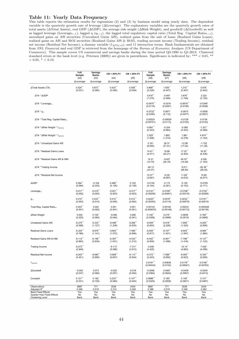
Table 11: Yearly Data FrequencyThis table reports the estimation results for regressions (2) and (3) by business model using yearly data. The dependentvariable is the quarterly growth rate of leverage (∆Leverage). The explanatory variables are the quarterly growth rates oftotal assets (∆Total Assets), real GDP (∆GDP), the average risk weight (∆Risk Weight), and goodwill (∆Goodwill) as wellas lagged leverage (Leveraget−1), lagged q (qt−1), the lagged total regulatory capital ratio (Total Reg. Capital Ratiot−1),unrealized gains on AfS securities (Unrealized Gains AfS), realized gains from the sale of loans (Realized Gains Loans),realized gains on AfS and HtM securities (Realized Gains AfS & HtM), trading account income (Trading Income), residualnet income (Residual Net Income), a dummy variable (1∆TA>0), and 11 interaction terms. Bank fundamentals are obtainedfrom SNL Financial and real GDP is retrieved from the homepage of the Bureau of Economic Analysis (US Department ofCommerce). This sample covers US commercial and savings banks during the time period Q3-1990 to Q1-2013. Clusteredstandard errors at the bank level (e.g. Petersen (2009)) are given in parentheses. Significance is indicated by: *** < 0.01, **< 0.05, * < 0.10.

Full Sample

Savings Banks

CB < 20% FV CB > 20% FV Full

SampleSavings Banks

CB < 20% FV CB > 20% FV

[42] [43] [44] [45] [46] [47] [48] [49] ∆Leverage ∆Leverage ∆Leverage ∆Leverage ∆Leverage ∆Leverage ∆Leverage ∆Leverage

∆Total Assets (TA) 0.524*** 0.873*** 0.423*** 0.558*** 0.868*** 1.055** 1.210*** 0.676* (0.031) (0.065) (0.048) (0.049) (0.229) (0.447) (0.407) (0.402) ∆TA * ∆GDP 3.618*** -0.497 3.676** 2.222 (1.270) (3.599) (1.746) (2.150) ∆TA * Leveraget-1 -0.0475*** -0.0316 -0.0618*** -0.0348* (0.0119) (0.0281) (0.0195) (0.0206) ∆TA * qt-1 -0.0722** 0.0871 -0.0815* -0.0836 (0.0340) (0.115) (0.0477) (0.0527) ∆TA * Total Reg. Capital Ratiot-1 0.00524 -0.00629 -0.0126 0.0138 (0.00701) (0.0113) (0.0153) (0.0120) ∆TA * ∆Risk Weight * 1(∆TA>0) -0.981*** -0.324 -0.369 -1.321**

(0.323) (0.864) (0.423) (0.568) ∆TA * ∆Risk Weight * 1(∆TA<0) 2.525** 1.893 1.981 4.974*** (1.008) (1.210) (2.278) (1.742) ∆TA * Unrealized Gains AfS 0.161 28.37 -12.96 -1.102 (8.505) (31.51) (17.02) (11.39) ∆TA * Realized Gains Loans 14.91*** 16.88 17.32*** 18.35** (4.471) (25.21) (5.402) (8.436) ∆TA * Realized Gains AfS & HtM 14.31 -9.427 45.33*** 4.036 (10.70) (26.19) (14.48) (7.183) ∆TA * Trading Income -46.13 9.511 -92.38*** (33.37) (56.90) (28.30) ∆TA * Residual Net Income 10.37*** 12.20 11.69** 10.80 (3.657) (9.097) (4.672) (6.577) ∆GDP 0.284*** -0.164 0.498*** 0.102 -0.0130 -0.172 0.126 -0.0759 (0.084) (0.225) (0.126) (0.139) (0.104) (0.261) (0.153) (0.171) Leveraget-1 -0.017*** -0.019*** -0.021*** -0.017*** -0.0141*** -0.0185*** -0.0168*** -0.0152*** (0.002) (0.005) (0.003) (0.003) (0.00206) (0.00461) (0.00319) (0.00288) qt-1 0.015*** 0.033*** 0.015*** 0.012*** 0.0220*** 0.0278** 0.0232*** 0.0191*** (0.003) (0.010) (0.005) (0.004) (0.00353) (0.0115) (0.00579) (0.00510) Total Reg. Capital Ratiot-1 0.003*** 0.002 0.001 0.001 0.00143 0.00192 0.00233 -0.000248 (0.001) (0.002) (0.001) (0.001) (0.000870) (0.00148) (0.00172) (0.00139) ∆Risk Weight 0.025 0.154** -0.006 0.006 0.149*** 0.219** 0.0639 0.189***

(0.025) (0.060) (0.040) (0.041) (0.0358) (0.0989) (0.0519) (0.0685) Unrealized Gains AfS -8.370*** -5.333*** -8.496*** -9.285*** -8.509*** -6.918*** -7.806*** -9.200*** (0.598) (1.127) (1.239) (0.635) (0.803) (2.228) (1.525) (0.859) Realized Gains Loans -6.324*** -8.876*** -5.603*** -7.485*** -6.935*** -8.727*** -6.603*** -8.964*** (0.786) (1.141) (1.072) (0.956) (0.817) (1.421) (1.097) (1.960) Realized Gains AfS & HtM -6.112*** -6.196*** -6.367*** -5.533*** -6.442*** -6.061*** -7.788*** -5.137***

(0.863) (0.934) (1.631) (1.212) (0.900) (1.098) (1.418) (1.122) Trading Income -8.472*** -9.113* -7.311* -3.049 -10.14** 7.445* (2.949) (5.098) (3.912) (4.425) (4.683) (4.058) Residual Net Income -6.203*** -8.085*** -5.808*** -6.113*** -6.372*** -7.588*** -6.093*** -6.330*** (0.421) (0.690) (0.607) (0.644) (0.423) (0.692) (0.623) (0.609) 1(∆TA>0) 0.0191*** 0.00838 0.0178*** 0.0156** (0.00434) (0.0122) (0.00647) (0.00762) ∆Goodwill -0.042 0.073 -0.025 -0.018 -0.0556 0.0467 -0.0439 -0.0244 (0.037) (0.060) (0.057) (0.040) (0.0364) (0.0643) (0.0567) (0.0413) Constant 0.121*** 0.182* 0.233*** 0.147*** 0.0886*** 0.180* 0.148** 0.121** (0.031) (0.100) (0.060) (0.045) (0.0325) (0.0928) (0.0621) (0.0467) Observations 6887 771 3536 2434 6887 771 3536 2434Adjusted R2 0.356 0.519 0.312 0.428 0.388 0.519 0.349 0.462 Bank Fixed Effects Yes Yes Yes Yes Yes Yes Yes Yes Quarter-Year Fixed Effects No No No No No No No No Clustering Level Bank Bank Bank Bank Bank Bank Bank Bank

44

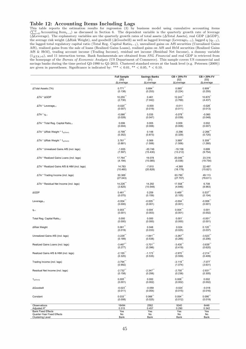
Table 12: Accounting Items Including LagsThis table reports the estimation results for regression (3) by business model using cumulative accounting items(∑2

i=0 Accounting Itemt−i) as discussed in Section 6. The dependent variable is the quarterly growth rate of leverage(∆Leverage). The explanatory variables are the quarterly growth rates of total assets (∆Total Assets), real GDP (∆GDP),the average risk weight (∆Risk Weight), and goodwill (∆Goodwill) as well as lagged leverage (Leveraget−1), lagged q (qt−1),the lagged total regulatory capital ratio (Total Reg. Capital Ratiot−1), unrealized gains on AfS securities (Unrealized GainsAfS), realized gains from the sale of loans (Realized Gains Loans), realized gains on AfS and HtM securities (Realized GainsAfS & HtM), trading account income (Trading Income), residual net income (Residual Net Income), a dummy variable(1∆TA>0), and 11 interaction terms. Bank fundamentals are obtained from SNL Financial and real GDP is retrieved fromthe homepage of the Bureau of Economic Analysis (US Department of Commerce). This sample covers US commercial andsavings banks during the time period Q3-1990 to Q1-2013. Clustered standard errors at the bank level (e.g. Petersen (2009))are given in parentheses. Significance is indicated by: *** < 0.01, ** < 0.05, * < 0.10.

Full Sample Savings Banks CB < 20% FV CB > 20% FV [50] [51] [52] [53] ∆Leverage ∆Leverage ∆Leverage ∆Leverage ∆Total Assets (TA) 0.771*** 0.684*** 0.565** 0.909*** (0.138) (0.253) (0.224) (0.255) ∆TA * ∆GDP 10.255*** 0.461 12.243*** 10.870** (2.730) (7.042) (3.769) (4.437) ∆TA * Leveraget-1 -0.020*** -0.000 -0.011 -0.026* (0.007) (0.019) (0.011) (0.013) ∆TA * qt-1 -0.066** 0.035 -0.078** -0.060 (0.028) (0.047) (0.039) (0.048) ∆TA * Total Reg. Capital Ratiot-1 0.006 0.005 0.009 0.002 (0.004) (0.006) (0.008) (0.007) ∆TA * ∆Risk Weight * 1(∆TA>0) -0.799** 0.148 -0.296 -2.266*** (0.352) (0.873) (0.329) (0.720) ∆TA * ∆Risk Weight * 1(∆TA<0) 3.761*** 0.569 3.569** 5.359*** (0.881) (1.506) (1.506) (1.260) ∆TA * Unrealized Gains AfS (incl. lags) -1.655 -20.746 -19.158 0.699 (7.597) (15.430) (13.212) (9.754) ∆TA * Realized Gains Loans (incl. lags) 17.764*** 19.078 20.046*** 23.316 (4.194) (15.085) (5.038) (19.754) ∆TA * Realized Gains AfS & HtM (incl. lags) 14.783 -7.810 -4.369 22.487 (10.460) (20.828) (18.178) (15.821) ∆TA * Trading Income (incl. lags) 50.369* 63.790** 49.113 (27.043) (27.707) (78.611) ∆TA * Residual Net Income (incl. lags) 14.226*** 14.292 17.558*** 6.708 (3.825) (10.548) (4.846) (8.983) ∆GDP 0.461*** 0.259 0.469*** 0.537*** (0.070) (0.159) (0.105) (0.104) Leveraget-1 -0.004*** -0.005*** -0.004*** -0.006*** (0.000) (0.001) (0.001) (0.001) qt-1 0.003*** 0.004* 0.004*** 0.001 (0.001) (0.003) (0.001) (0.002) Total Reg. Capital Ratiot-1 0.000 0.000 0.001* -0.001** (0.000) (0.000) (0.000) (0.001) ∆Risk Weight 0.061*** 0.048 0.024 0.120*** (0.019) (0.033) (0.025) (0.037) Unrealized Gains AfS (incl. lags) -3.229*** -1.841*** -3.267*** -3.523*** (0.189) (0.538) (0.266) (0.206) Realized Gains Loans (incl. lags) -3.467*** -3.701*** -3.430*** -3.639*** (0.277) (0.396) (0.419) (0.620) Realized Gains AfS & HtM (incl. lags) -2.155*** -1.173** -2.970*** -2.214*** (0.320) (0.535) (0.559) (0.409) Trading Income (incl. lags) -3.794*** -3.119*** -7.077* (0.992) (1.074) (3.631) Residual Net Income (incl. lags) -2.732*** -2.347*** -2.750*** -2.831*** (0.158) (0.206) (0.238) (0.305) 1(∆TA>0) 0.005*** 0.000 0.008*** 0.002 (0.001) (0.002) (0.002) (0.002) ∆Goodwill -0.023** -0.059 -0.024* -0.018 (0.011) (0.054) (0.015) (0.016) Constant 0.033*** 0.066*** 0.054*** 0.090*** (0.008) (0.025) (0.012) (0.019) Observations 18494 2562 9340 6446 Adjusted R2 0.315 0.457 0.290 0.342 Bank Fixed Effects Yes Yes Yes Yes Quarter-Year Fixed Effects No No No No Clustering Level Bank Bank Bank Bank

45

Table

13:

Bala

nce

Sheet

Exp

an

sion

san

dC

ontr

act

ions

Th

ista

ble

rep

ort

sth

ees

tim

ati

on

resu

lts

for

regre

ssio

n(3

)by

bu

sin

ess

mod

el,

dis

tin

gu

ish

ing

bet

wee

nb

ala

nce

shee

tex

pan

sion

san

dco

ntr

act

ion

sfo

rth

eb

ase

lin

em

od

elas

wel

las

the

ver

sion

sw

ith

lagged

acc

ou

nti

ng

item

san

dyea

rly

data

.T

he

dep

end

ent

vari

ab

leis

the

qu

art

erly

gro

wth

rate

of

lever

age

(∆L

ever

age)

.T

he

exp

lan

ato

ryvari

ab

les

are

the

qu

art

erly

gro

wth

rate

sof

tota

lass

ets

(∆T

ota

lA

sset

s),

real

GD

P(∆

GD

P),

the

aver

age

risk

wei

ght

(∆R

isk

Wei

ght)

,an

dgood

will

(∆G

oodw

ill)

as

wel

las

lagged

lever

age

(Lev

erage t

−1),

lagged

q(q

t−1),

the

lagged

tota

lre

gu

lato

ryca

pit

al

rati

o(T

ota

lR

eg.

Cap

ital

Rati

ot−

1),

un

realize

dgain

son

AfS

secu

riti

es(U

nre

alize

dG

ain

sA

fS),

realize

dgain

sfr

om

the

sale

of

loan

s(R

ealize

dG

ain

sL

oan

s),

realize

dgain

son

AfS

an

dH

tMse

curi

ties

(Rea

lize

dG

ain

sA

fS&

HtM

),tr

ad

ing

acc

ou

nt

inco

me

(Tra

din

gIn

com

e),

resi

du

al

net

inco

me

(Res

idu

al

Net

Inco

me)

,a

du

mm

yvari

ab

le(1

∆T

A>

0),

an

d15

inte

ract

ion

term

sas

dis

cuss

edin

Sec

tion

6.

Ban

kfu

nd

am

enta

lsare

ob

tain

edfr

om

SNL

Financial

an

dre

al

GD

Pis

retr

ieved

from

the

hom

epage

of

theBureauofEconomic

Analysis

(US

Dep

art

men

tof

Com

mer

ce).

Th

issa

mp

leco

ver

sU

Sco

mm

erci

al

an

dsa

vin

gs

ban

ks

du

rin

gth

eti

me

per

iod

Q3-1

990

toQ

1-2

013.

Clu

ster

edst

an

dard

erro

rsat

the

ban

kle

vel

(e.g

.P

eter

sen

(2009))

are

giv

enin

pare

nth

eses

.S

ign

ifica

nce

isin

dic

ate

dby:

***<

0.0

1,

**<

0.0

5,

*<

0.1

0.

B

asel

ine

Mod

el

Acc

ount

ing

Item

s In

clud

ing

Lags

Ye

arly

Dat

a

Full

Sam

ple

Savi

ngs

Ban

ksC

B <

20%

FV

CB

> 2

0% F

V Fu

ll Sa

mpl

eSa

ving

s B

anks

C

B <

20%

FV

CB

> 2

0% F

V Fu

ll Sa

mpl

e Sa

ving

s B

anks

C

B <

20%

FV

CB

> 2

0% F

V

[54]

[5

5]

[56]

[5

7]

[58]

[5

9]

[60]

[6

1]

[62]

[6

3]

[64]

[6

5]

∆

Leve

rage

∆

Leve

rage

∆Le

vera

ge∆

Leve

rage

∆Le

vera

ge∆

Leve

rage

∆

Leve

rage

∆Le

vera

ge∆

Leve

rage

∆Le

vera

ge∆

Leve

rage

∆Le

vera

ge

∆

Tota

l Ass

ets

(TA)

0.

940**

* 0.

699**

* 0.

891**

* 0.

888**

* 0.

768**

* 0.

721**

* 0.

572**

0.

907**

* 0.

873**

* 1.

043**

1.

201**

* 0.

734*

(0

.109

) (0

.213

) (0

.143

) (0

.174

) (0

.139

) (0

.261

) (0

.225

) (0

.254

) (0

.231

) (0

.452

) (0

.411

) (0

.404

)

∆

TA * ∆

GD

P *

1(∆

TA>0

) 7.

210**

-0

.326

8.

840*

6.59

0 11

.285

***

4.88

7 14

.341

***

10.8

84**

3.42

5**

0.03

1 2.

492

3.01

1

(3.1

74)

(7.0

77)

(4.5

29)

(5.2

18)

(3.4

43)

(8.9

47)

(4.7

31)

(5.4

64)

(1.3

37)

(4.2

60)

(1.8

44)

(2.2

88)

∆

TA * ∆

GD

P *

1(∆

TA<0

) 9.

233**

-1

.822

9.

767

15.4

79*

5.38

4 -1

2.88

5 3.

174

11.5

32

5.74

3 -5

.237

14

.764

**

-2.9

78

(4

.560

) (7

.171

) (6

.832

) (8

.849

) (4

.970

) (9

.009

) (7

.207

) (7

.471

) (4

.127

) (9

.090

) (6

.564

) (6

.799

)

∆

TA *

Lev

erag

e t-1

-0.0

24**

* 0.

001

-0.0

21**

* -0

.020

**

-0.0

20**

* -0

.001

-0

.011

-0

.026

* -0

.048

***

-0.0

31

-0.0

62**

* -0

.038

*

(0.0

06)

(0.0

16)

(0.0

08)

(0.0

09)

(0.0

07)

(0.0

19)

(0.0

11)

(0.0

13)

(0.0

12)

(0.0

28)

(0.0

20)

(0.0

21)

∆

TA *

q t-1

-0.0

44*

0.02

9 -0

.054

* -0

.067

**

-0.0

67**

0.03

5 -0

.082

**

-0.0

62

-0.0

74**

0.09

1 -0

.076

-0

.089

*

(0.0

24)

(0.0

41)

(0.0

32)

(0.0

32)

(0.0

28)

(0.0

52)

(0.0

39)

(0.0

47)

(0.0

34)

(0.1

18)

(0.0

48)

(0.0

53)

∆

TA *

Tot

al R

eg. C

apita

l Rat

io

0.00

1 0.

006

-0.0

00

0.00

3 0.

006

0.00

4 0.

008

0.00

2 0.

005

-0.0

07

-0.0

11

0.01

2

(0.0

03)

(0.0

06)

(0.0

04)

(0.0

05)

(0.0

04)

(0.0

06)

(0.0

08)

(0.0

07)

(0.0

07)

(0.0

11)

(0.0

15)

(0.0

12)

∆

TA * ∆

Ris

k W

eigh

t * 1

(∆TA

>0)

-0.6

08*

-0.0

17-0

.387

-1.5

54**

*-0

.818

**0.

334

-0.3

26-2

.300

***

-0.9

67**

*-0

.258

-0.3

33-1

.329

**

(0

.348

) (0

.612

) (0

.351

) (0

.593

) (0

.354

) (0

.823

) (0

.332

) (0

.720

) (0

.323

) (0

.910

) (0

.420

) (0

.556

)

∆

TA * ∆

Ris

k W

eigh

t * 1

(∆TA

<0)

2.92

8***

0.57

9 3.

177**

3.

298**

* 3.

984**

* 1.

150

3.77

6**

5.21

9***

2.50

7**

1.90

6 1.

393

5.51

9***

(0

.747

) (1

.208

) (1

.277

) (1

.032

) (0

.923

) (1

.523

) (1

.613

) (1

.265

) (1

.001

) (1

.266

) (2

.258

) (1

.771

)

∆

TA *

Unr

ealiz

ed G

ains

AfS

* 1 (

∆TA>

0)

5.83

0 -1

1.96

5 -2

4.82

1 8.

870

-5.3

42

-9.1

30

-31.

712*

-1.9

10

2.75

6 49

.731

-6

.189

-2

.561

(12.

061)

(4

2.12

7)(2

7.61

1)(1

3.71

6)(9

.300

)(2

0.40

0)

(18.

294)

(11.

826)

(9.6

86)

(40.

850)

(20.

851)

(13.

596)

∆

TA *

Unr

ealiz

ed G

ains

AfS

* 1 (

∆TA<

0)

-30.

094

-26.

336

9.65

3 -1

4.45

2 8.

307

-51.

115

33.0

83

9.11

5 -2

1.43

8 -7

3.38

1 -1

08.3

58

26.4

16

(2

6.21

7)

(23.

752)

(4

0.81

2)

(26.

499)

(1

5.43

3)

(47.

501)

(2

5.05

1)

(16.

180)

(3

1.85

3)

(71.

792)

(7

8.10

7)

(30.

911)

∆

TA *

Rea

lized

Gai

ns L

oans

31

.905

***

47.5

89**

33.5

27**

* 22

.046

17

.658

***

17.4

10

20.1

41**

* 23

.837

15

.022

***

15.2

53

17.9

40**

* 16

.713

*

(8.3

20)

(18.

619)

(9

.776

) (3

4.91

5)

(4.2

23)

(15.

552)

(5

.104

) (1

9.77

1)

(4.4

88)

(25.

177)

(5

.360

) (9

.086

)

∆

TA *

Rea

lized

Gai

ns A

fS &

HtM

* 1 (

∆TA>

0)

29.1

40

2.73

3 29

.905

26

.634

19

.350

45

.717

-2

8.60

6 14

.826

17

.177

-1

1.71

2 59

.190

***

-1.1

60

(2

8.31

9)

(24.

688)

(4

5.44

5)

(44.

361)

(1

3.57

5)

(32.

799)

(3

2.00

1)

(16.

301)

(1

2.60

1)

(25.

878)

(1

2.20

5)

(8.1

00)

∆

TA *

Rea

lized

Gai

ns A

fS &

HtM

* 1 (

∆TA<

0)

2.23

4 -2

3.72

7 -5

.697

29

.185

8.

806

-71.

081

39.6

31

51.5

72

-19.

791

67.8

18

-72.

042

62.7

71**

(2

9.89

0)

(44.

056)

(4

0.12

7)

(53.

628)

(2

6.15

3)

(43.

526)

(3

2.15

8)

(38.

582)

(3

1.26

4)

(120

.321

) (4

8.95

2)

(31.

572)

∆

TA *

Trad

ing

Inco

me

* 1(∆

TA>0

)13

4.41

8 21

6.94

3**33

.123

69.6

3512

5.95

2**-7

.379

-20.

061

17.0

42-7

5.88

6

(89.

701)

(87.

449)

(1

72.3

46)

(53.

343)

(57.

819)

(1

05.1

64)

(35.

210)

(55.

655)

(6

3.48

8)

∆

TA *

Trad

ing

Inco

me

* 1(∆

TA<0

) -9

3.92

4

-262

.536

16

68.7

05**

* 14

.336

-33.

530

251.

871

-226

.282

*

-87.

017

-157

.347

(234

.261

)

(255

.613

) (5

89.4

32)

(48.

484)

(60.

586)

(1

57.0

90)

(120

.044

)

(177

.759

) (1

68.9

47)

∆

TA *

Res

idua

l Net

Inco

me

19.7

52**

13.8

00

22.6

77**

14.8

94

14.0

23**

* 14

.138

17

.569

***

7.30

0 10

.462

***

11.6

56

11.9

57**

* 10

.627

(7.8

50)

(11.

744)

(9

.795

) (1

4.19

1)

(3.8

44)

(10.

576)

(4

.889

) (9

.048

) (3

.640

) (9

.472

) (4

.584

) (6

.509

)

Obs

erva

tions

21

581

3020

10

984

7402

18

494

2562

93

40

6446

68

87

771

3536

24

34

Adju

sted

R2

0.46

6 0.

596

0.39

00.

567

0.31

50.

460

0.29

00.

342

0.38

90.

519

0.35

10.

463

Sta

nd-A

lone

Var

iabl

es

Yes

Yes

Yes

Yes

Yes

Yes

Yes

Yes

Yes

Yes

Yes

Yes

Ban

k Fi

xed

Effe

cts

Yes

Yes

Yes

Yes

Yes

Ye

s Ye

s Ye

s Ye

s Y

es

Yes

Yes

Qua

rter-

Year

Fix

ed E

ffect

s N

o N

o N

o N

o N

o N

o N

o N

o N

o N

o N

o N

o C

lust

erin

g Le

vel

Bank

Ba

nk

Bank

Ba

nk

Bank

Ba

nk

Bank

Ba

nk

Bank

Ba

nk

Bank

Ba

nk

46

Figure 3: Time-Series of Leverage, Capital Ratios and Total AssetsThis figure shows the evolution of leverage, capital ratios and total assets from Q3-1990 to Q1-2013 forthe average (equally weighted) US commercial and savings bank. Leverage is defined as the ratio of totalassets to total book equity. The tier 1 and the total regulatory capital ratio are given in percent. Totalassets are denoted in US$ billion. The data is obtained from SNL Financial.

0

5

10

15

20

7

9

11

13

15

17

1990 1993 1995 1998 2000 2003 2005 2008 2010 2013

Leverage Tier 1 Capital Ratio Total Reg. Capital Ratio Total Assets

Full Sample

Levera

ge a

nd C

apital R

atios

To

tal A

sse

ts (

US

$ b

n.)

47