procyclicality in basel iii in the visegrád countries · hypothesis 2: the correlation between gdp...
TRANSCRIPT

663
Procyclicality in Basel III in the Visegrád Countries
Petra Šobotníková
Charles University in Prague, Czech Republic
Institute of Economic Studies, Faculty of Social Science
Opletalova 26
Prague 110 00
Czech Republic
e-mail: [email protected]
Petr Teplý
Charles University in Prague, Czech Republic
Institute of Economic Studies, Faculty of Social Science
Opletalova 26
Prague 110 00
Czech Republic
e-mail: [email protected]
Abstract
The term procyclicality refers to the ability of a system to amplify business cycles. The recent financial
crisis has revealed that the current bank regulatory framework Basel II affects the business cycle in
exactly that manner. As a result, the newly published Basel III has introduced tools that should
mitigate the procyclical nature of regulatory framework. As the Basel III framework was published in
December 2010, there are few studies analyzing its effect on procyclicality. The aim of the paper is to
analyze whether the new tools are effective and whether the procyclicality under Basel III has been
mitigated compared to Basel II. We employ a regression model with households and firm sector in
order to conduct such analysis. Using the OLS estimation method we estimate the sensitivity of Basel
risk weights to the business cycle under both Basel II and Basel III conditions. The main contribution
of this paper consists of implementation of Basel III countercyclical tools and of comparison between
both frameworks. The paper further contributes to the existing literature by conducting the analysis on
the data for the Visegrád Group (the Czech Republic, Slovakia, Hungary and Poland). When applying
a standard regulatory formula, we show that results for Hungary differ greatly from the rest of the
region as this country has shown a completely different pattern in the input data. This conclusion that
regulatory rules cannot be applied generally for all countries should be appealing for both regulators
and bankers.
Keywords: procyclicality, Basel II, Basel III, banking supervision
JEL codes: E32, E44, E58, G21
1. Introduction (First-level heading, Times New Roman 11, bold)
The global crisis has raised many talks about bank regulatory framework and revealed that
current rules for supervision are not sufficient as they failed to predict or even avoid such a crisis. As a
result, a revision of current banking regulation Basel II was needed to reflect the current trends in the
world financial markets and in December 2010 the Basel Committee on Banking Supervision (BCBS)
issued new proposals for international bank regulation Basel III. One of the objectives of Basel III is,
among others, to mitigate the procyclicality of the previous banking regulation framework Basel II.
Under a Basel II capital adequacy formula the required amount of capital was assumed to grow in
times of economic downswing and vice versa. With a higher amount of capital necessary to keep as a
capital adequacy banks may offer less credits and force the economy deeper into recession. Put

664
differently, Basel II has reported procyclicality what was demonstrated by Gordy and Howells (2004),
Gerali et al. (2009) or Angelini et al. (2010).
The aim of this paper is to analyze how much procyclicality has been mitigated under the new
rules Basel III compared to Basel II. We will analyze it on a macroeconomic level concentrating on
the Visegrad countries (the Czech Republic, Slovakia, Poland and Hungary) by comparing
development of the risk weights of Basel capital adequacy to the business cycle for both regulatory
frameworks. We will examine three hypotheses. A first hypothesis states that there is a strong negative
correlation between the business cycle and the risk weights for Basel II. A second hypothesis assumes
that such correlation will be weaker for Basel III framework. A final hypothesis verifies whether the
effect of Basel Accords differs in different the countries towards the financial crisis.
The paper continues as follows. In the next section we review and report on some of the
previous research that has looked at procyclicality under Basel I and Basel II. Section 3 looks in more
detail at the applied methodology. In Section 4 we provide empirical analysis of procyclicality under
both Basel II and Basel III the Visegrad countries. Section 5 concludes the paper and states final
remarks.
2. Literature Review
In recent years many studies covering this topic with respect to Basel II have been published
such as Lall (2009) or Teplý (2010). Immediately after the release of Basel II in 2004, many experts
started to deliver analyses of the possible impact of more risk sensitive approach on the economy. All
the studies were driven by the same concern emerging from the stronger link between risk exposure
and capital. Should the loans during an economic downturn become more risky, banks would be
required to hold more regulatory capital which would negatively affect their willingness to grant
further credits and would deepen the recession. Such concerns further increased after the start of the
crisis. The procyclicality might be researched on two main levels: and on portfolio level or on
macroeconomic level, what is the core of our study. For more details on the research of procyclicality
we refer to the works Kashyap and Stein (2004), Repullo, Saurina and Trucharte (2009), Saurina
(2009) or Varsanyi (2007).
In this paper we analyze potential procyclicality rather on macroeconomic level, what has not
been done by many studies, however. For instance, Gerali et al. (2009) set their study into a dynamic
stochastic general equilibrium model (DSGE) that is into an equilibrium model which explains
economic variables on macroeconomic level while being derived from microeconomic principles. As
the name of the model suggests, DSGE explains the evolution of economic variables over time and
takes into account random shocks. The main advantage of such model is that DSGE does not yield to
the Lucas critique. DSGE models incorporating financial frictions have been first introduced at the end
of 1990s but have not actively included any financial intermediaries such as banks.
Gerali et al. (2009) contributed substantially to the DSGE literature as they provide first model
which incorporates banking sector and therefore connect credit and financial markets. This allows to
“understand the role of banking intermediation in the transmission of monetary impulses and to
analyze how shocks originate in credit markets and are transmitted to the real economy” (Gerali et al.,
2009). The model presented in the paper covers simple economy populated by households and firms
and complemented by banks and central bank and introduces set of equations which describe basic
relationships in the economy related to utility maximization, loan and deposit demand, interest rate
setting and labor market. Linearized model of equations then uses the Bayesian approach to estimate
its parameters. Authors use data from the years 1998 to 2008, de-trended by the Hodrick-Prescott
filter. Gerali et al. (2009) further use the estimated parameters to study the dynamics of the model.
They do so through the use of impulse response functions. Impulses induced to the model are
monetary policy shock and technology shock. A paper presented by Gerali et al. (2009) serves as a
starting point to the paper from Angelini et al. (2010), who adopted this model and extended it with
risk weights. Having calculated the required capital and corresponding risk weights the authors use
regression to estimate risk sensitivity of risk weights on the business cycle. To approximate
probabilities of default delinquency rates for US loans are used. The authors then compare the
procyclicality of Basel I and Basel II with impulse response functions, testing the sensitivity of
economy on positive technological shock as well as positive monetary policy shock. The functions are

665
based on parameters of DSGE model estimated by Gerali et al. (2009). The results clearly show the
pronounced procyclicality of Basel II when compared to economy under Basel I regulatory regime.
However, the extent of added procyclicality obtained by Angelini et al. (2010) is not as large as
expected.
When analyzing the proposed tools to mitigate procyclicality of Basel II the authors study
impulse response functions for positive technology shock and expansionary monetary policy shock
under the regime of passive countercyclical requirements with time varying capital ratio and
alternative regulatory regimes.
3. Methodology
Our model is partially based both on Angelini et al. (2010) and Gerali et al. (2009). Both
studies have incorporated banking sector into the DSGE framework and Angelini et al. (2010)
included risk weights to analyze the impact of Basel II capital regulation. We adopt the economy
settings presented in those papers. The aim of the paper is to broaden the model to incorporate Basel
III changes and compare the procyclicality of both regulatory frameworks. Throughout the model we
approximate the cyclical conditions with the changes in GDP. Such an approximation is reflected in
the formulation of the hypotheses the paper has stipulated. Our hypotheses are as follows:
Hypothesis 1: Basel II rules reports a strong negative correlation between GDP and the risk
weighted assets.
This hypothesis covers the expected procyclicality of Basel II with the business cycle being
approximated by the GDP development. If Basel II is procyclical, the risk weights will grow as a GDP
will decrease.
Hypothesis 2: The correlation between GDP and risk weighted assets will be less negative for
Basel III framework.
This hypothesis reflects the assumption of lower procyclicality of Basel III in comparison to
Basel II.
Hypothesis 3: Effect of Basel II and Basel III proposals on procyclicality will differ among the
countries.
Given the knowledge about recent economic development and policies in the countries
observed we assume that the procyclicality and its change will not be the same among all countries of
the region.
As already mentioned, setting the analysis into DSGE framework provides us with the opportunity to measure the impact of both Basel II and Basel III rules on a macro level. It does not
yield to the Lucas critique and connects the model to the real economy. There have been many studies
published proving the procyclicality of Basel II such as Angelini et al. (2010), Gerali et al. (2009) or
Šobotníková (2011). We therefore focus on comparison between Basel II and Basel III. To start our
analysis let us assume simple model within an economy with four key players: households (HH), firms
(F), banks (B) and monetary authority. There are two types of households which differ in their degree
of patience. Patient households prefer future consumption and save money in form of deposits while
impatient households prefer current consumption and take loans from banks. Simple economy coheres
with a simple balance sheet of banks. The asset side of the banking sector is composed of loans to
firms and impatient households while the liabilities side consists of household deposits and capital.
The budget constraint of banks is captured in (1):
(1)
where denotes loans to households at time t,
- loans to firms at time t, - deposits at
time t and - capital at time t.
Both Basel Accords set minimal a capital-to-assets ratio . When banks deviate from this ratio
they face a cost in quadratic form given by (2):
(1)
666
where measures the bank capital in time t, C is the corresponding cost in time t and is the
parameter assigned to the cost of deviating from optimal capital-to-assets ratio. The real capital-to-
assets ratio is adjusted for risk weights separately for households and for firms and denoted as
and respectively. Both Basel II and Basel III let the risk weights vary over time in order to capture
the changing risks in the economy. As Angelini (2010) points out, setting
would
approximate the risk insensitive setting of the original Basel 1 framework.
3.1 Basel II model
In order to assess the procyclicality of Basel II and Basel III we analyze the correlation
between the risk weights and the business cycle. Let us assume that the risk weights are subject to a
motion in form given by (3):
(3)
Through this equation we presume the risk weights to be dependent on cyclical conditions
approximated by the year-on-year change in output.1 We also presume some persistence in the risk
weights adjustment represented by the previous value of risk weights . The parameter in the
equations measures just the sensitivity to cyclical conditions which is of particular importance to our
study. The parameter determines the level of persistence in the model as it multiplies the previous
value of risk weights.
Since Basel II has been effective only for short period of time there are no time series for risk
weights that would satisfy our model. Therefore we have to calculate them based on the Basel
formulae for capital adequacy. Both Basel II and Basel III specify exact formula to calculate required
capital on loans as provided in (4).
(2)
According to the formula, the required capital is a function of probability of default PD, loss
given default LGD and the correlation parameter .2 In both the Standard approach and the foundation
IRB approach LGD is given by supervisors. We assume and , what
follows Gerali et al. (2009). Regarding the correlation parameter Basel Accords specify its calculation
depending on the size of the creditor. For firms we have used the formula for small and medium-sized
enterprises (SMEs) in (5).
(Chyba! Záložka není
definována.)
Households in this paper follow the formula for retail exposures defined in (6).
(Chyba! Záložka není
definována.)
Under Basel II the capital adequacy ratio is set to 8%. Therefore we can finally compute risk
weights as:
(7)
1 As it will be explained in the next part we are working with quarterly data. Therefore the year-on-year change
in output is measured as 2 For simplicity and due to the fact that we build the model on macroeconomic level and do not work with
portfolios of individual banks we neglect the effect of maturity.

667
This process provides us with time series of risk weights.3 As we have already mentioned
setting them up into regression we can estimate the sensitivity of the risk weights to the business cycle
for both households and firms under the Basel II framework.
3.2. Basel III innovation
The main reason for replacing Basel II with new framework was to respond to the financial
crisis with tightening regulatory and supervisory rules. BCBS (2010a) and BCBS (2010b) developed
the new framework to improve the ability of banking sector to absorb shocks and to reduce spillovers
as well as to address lessons of the financial crisis. The new framework works on both micro- and
macro-prudential level. On micro-prudential level it strives for higher resilience of individual banks
while from macro-prudential point of view the focus is on system-wide risks. The framework is based
on the three pillars introduced in Basel II but strengthened (BCBS, 2010a).
The first key area encompasses higher quality, consistency and transparency of capital base,
while higher risk coverage is the second key area of Basel III (e.g. counterparty risk). The third key
area is the capital conservation buffer. The main idea is to motivate banks to build up enough capital
reserves in times of prosperity which can then be used in times of crisis. The minimum limit for
capital conservation buffer is 2.5% of Tier 1 capital. This percentage cannot however be counted into
regulatory minimum capital. Banks first have to keep 6% of Tier 1 and 8% of total capital adequacy
and only then can use the excessive capital to build the conservation buffer.
There is also a second type of buffer defined under Basel III. It is a countercyclical buffer,
extension to the capital conservation type. The buffer was designed with the aim to reduce
procyclicality. As we have already discussed the financial crisis has revealed the effect of procyclical
amplification supported among others through accounting standards and handling of leverage.
Therefore Basel III developed countercyclical measures to enhance shock absorption instead of
transmission and amplification. It serves also as a tool against the trade-off between risk sensitivity
and cyclicality. As we know the more the regulation is risk sensitive the higher is the procyclicality
effect. This trade-off was already known when developing Basel II framework but the measures taken
to deal with were not sufficient. This may be due to one of the main criticisms of Basel II. It was
developed in times of prosperity and the rules were not adequate for crisis times. Now the BCBS
suggests stronger provisioning, further conservation of capital which can be used in times of crisis and
mechanisms which would adjust capital buffer when signs of excessive credit growth would be
identified.
Basel III sets the rules for each bank on how to set the buffer with respect to their jurisdiction.
For internationally active banks the principle of juridical reciprocity applies. This means that a bank
has to obey the decisions of an authority of the country where the bank operates. Banks should
subsequently calculate weighted average of buffers of all jurisdictions, where they file credit exposure.
The responsibility of home authority of an internationally active bank is to ensure that bank calculates
the buffer correctly. Home authority can further increase the buffer if it considers current level
insufficient or set the buffer entirely when host authority does not do so. Most of the key areas of
Basel III put requirements on Tier 1 as well as on total capital. BCBS (2010c) keeps the adequacy
ratio for total capital remained unchanged at 8%. However, when adding the requirement for
Conservation buffer (consisting purely from common equity Tier 1 capital) the total capital
requirements rise to 10.5%. As mentioned, the countercyclical buffer has been developed into Basel
III to mitigate the procyclicality of the current framework. To address the procyclicality of Basel III
we will add the buffer into the previous model. BCBS (2010c) sets that the decision about imposition
of the countercyclical buffer and its release is in hands of national authorities. However, the
Committee sets some guidelines for such determination. Among the most important guidelines is the
ratio of credits to GDP. To translate the ratio to the buffer, we follow the steps described in BCBS
(2010c).
First we calculate the actual ratio of credits to private sector to the GDP. This ratio is then
translated into trend using Hodrick-Prescott filter. BCBS (2010) sets the smoothing parameter to the
3 The literature usually defines the capital adequacy ratio as a ratio of capital to RWA. We would arrive to RWA
as RWA=w*EAD.

668
value of 400,000 to capture the long term trend. 4 In our model is set to the value of 50,000 as we
have data, that capture rather short period; ranging from Q1 1993 to Q1 2010. The actual level of
buffer is derived from the gap between the ratio and its trend as in (8).
(8)
To translate the gap into the buffer every national authority sets upper and lower value of the
gap which will correspond with the upper and lower level of the buffer. The countercyclical buffer is
defined in the range between 0 and 2.5%. The lower bound (L) is the level when a higher buffer than
0% should be imposed while the upper bound (H) signals that the highest buffer possible, 2.5% will be
imposed. For our model L equals to gap of 5 and H is set to the gap equal to 15. This means that:
for the countercyclical buffer is set to 0%
for the countercyclical buffer is set to 2.5%
for the countercyclical buffer varies linearly between
0 and 5%
As it was said before, the decision about the value of the bounds is in hands of national
authorities. BCBS (2010) only observes that empirically the values of L=2 and H=10 have proven to
be the most appropriate. Since we are working with data covering shorter period of time, we have
shifted the values to L=5 and H=15. When adding the buffer to the capital requirements we change the
constant minimal capital-to asset ratio to a variable one. The new minimal capital-to-asset ratio will vary between 8% and 10.5% and its variation will depend on the level of countercyclical buffer
imposed.
Variable changes the calculation of risk weights in our model. For Basel III model we still
follow the steps described through Equations (4), (5) and (6) The change follows when transforming
the calculated capital into the risk weights. For Basel II we obtain:
For Basel III we need to add the buffer and achieve time varying capital requirements.
Therefore, the Basel III risk weights are to be calculated as follows:
The new time series of risk weights obtained through employing Basel III countercyclical
buffer are again analyzed for sensitivity to business cycles. The regression formula is similar with the
regression formula (3) for Basel II and formulated in (8):
(8)
The parameter now stands for sensitivity of the Basel III risk weights to the business cycle.
Comparing it to the Basel II sensitivity parameter provides us with the result to the question
whether Basel III mitigates the procyclicality of the regulation.
4. Empirical Analysis
4.1 Data
The model of this paper is based on data for the region of the Visegrád Group (the Czech
Republic, Slovakia, Hungary and Poland). We analyze quarterly data ranging from the first quarter of
2002 to the first quarter of 2010. That allows us to observe the cyclical behavior of both Basel
Accords during a period of prosperity and growth as well as during a recession which is represented
by the recent financial crisis. The calculation of capital requirements and consequently risk weights is
based on PD and LGD. As it has been mentioned in the methodological part we assume LGD to be
4 BCBS (2010) does not specify the appropriate time range for calculation of long-term trend. However, in its
example for calculation of the buffer BCBS (2010) employs data for period 1963 to 2009.

669
given by the regulator and set its value in accordance with Gerali (2009) to LGDHH
=20% and
LGDF=40%. As for the probabilities of default it is difficult to collect data that would represent PDs
on macro level as each bank calculates its own values for PDs of its portfolio. Bearing in mind that
default is actually a migration from performing to non-performing loans we approximate PDs with
data on non-performing loans. NPL represents a loan which payments are overdue for 90 days or
more. Our data represent the ratio of NPLs to total loans separately for households and non-financial
corporations and were collected from Stability Reports of Central Banks of the region.
As for the output we employ quarterly data on nominal GDP in national currencies from the
IMF database. Figure 5 in Appendix compares the development of NPLs for both households and
firms. Looking at the data suggests that there is a procyclicality effect for Czech Republic and
Slovakia, more pronounced for firms than for households. This should be supported by negative
correlation of GDP and risk weights in next section. For Hungary and Poland the correlation is not to
obvious due to different development of both countries during the period observed. While GDP of
Hungary displays similar trend to GDP in the Czech Republic and Slovakia, the NPLs develop
differently. Hungarian NPLs for both households and firms do not show the bowed shape typical for
NPLs in the rest of the region as the levels of NPLs in both household and firms sector remain on low
levels and do not start to rise until the financial crisis. However, after the onset of the crisis they rise
more than in the rest of the region. Poland, on the other hand, follows the trend for NPLs with high
levels at the beginning of the observed period and again with the start of the crisis but its GDP does
not display any stronger decrease as a consequence of the financial turmoil. One last thing important
to notice and which should be reflected in the estimation results is that Hungary does not display
substantial differences between NPLs for households and for firms, except for the past couple of years.
For the second part of the model which is the calculation of capital buffer we use quarterly
data on claims after private sector for the period 1Q 1993 to 1Q 2010. The chosen period is longer
than the period examined in procyclicality in order to be able to capture trend in the evolution of the
credit-to-GDP ratio. Basel III procyclicality analysis proceeds as a simulation of Basel III rules on
existing data. Therefore no new dataset is required. We develop our analysis with the data on NPLs
and nominal GDP from 1Q 2002 to the 1Q 2010 amended by the countercyclical buffer which has
been computed based on the data for claim after private sector and again nominal GDP for the period
1Q 1993 to 1Q 2010 to capture the trend
4.2 Results
4.2.1 Procyclicality of Basel II
As the methodology suggests the first task was to obtain risk weights for both household and
firm loans. Based on data for NPLs and using Basel II formula we have obtained time series of risk
weights for households and corporations. When comparing the risk weights to non-performing loans (
Figure 1), we can see that the trend is identical to comparison of GDP and NPL in Figure 5 in
Appendix. This is a result of the fact that probabilities of default are the core item for risk weights
calculation (and in our case PDs are approximated by NPLs).

670

671
Figure 1: Comparison of risk weights and GDP from 4Q 2002 to 1Q 2010
Source: Authors’ calculations

672
With risk weights following the same pattern as NPLs, our observations from the previous
section about the development of variables in respective countries remains valid.
Figure 1 displays a strong indication that the results for Hungary will differ from the rest of
the region due the unique development of the country. With the time series of risk weights we have
then carried out the regression analysis for risk weights under Basel II. Results of the OLS estimation
correspond to the observations we have made based on just visual comparison of the data for NPLs
and GDP in Figure 5 in Appendix. The complete results with the exact regression output from the
Gretl software together with tests for assumptions are enclosed in Appendix. The aim was to estimate
the coefficient for sensitivity of risk weights to the business cycle for both households and firms
model. Table 1 presents the results of coefficient estimation for the household model.
Table 1: Estimation results for the household model under Basel II
Source: Authors’ calculations
Note:***denotes significance on a 1% level.
With the exception of Hungary the estimation shows negative values of parameter for all
countries. The estimation displays high level of statistical significance for all countries except for
Poland where the p-value is higher than 0.05. The coefficient of determination ranges from
77.14% to 97.59% suggesting a solid goodness of fit. As to the assumptions of the model, based on the
test of White (1980) for heteroskedasticity the hypothesis of homoskedasticity is rejected for the
Czech Republic. Heteroskedastic data should not have influence on the estimation values itself but
could influence other statistics so the results about statistical significance have to be interpreted with
some caution. The hypotheses of no collinearity and normal distribution of residuals cannot be
rejected for any of the countries. Based on Durbin and Watson (1951) the Durbin-Watson statistics is
sufficiently close to 2 for Slovak households and we cannot reject the hypothesis of no autocorrelation
of disturbances. For the rest of the countries the Durbin-Watson statistics displays lower values. We
have therefore checked the autocorrelation of disturbances with the Breusch-Godfrey test (Breusch
1979, Godfrey 1978). Again, we cannot reject the hypothesis that no autocorrelation is present. Exact
results of the tests performed are stated in Appendix 1.

673
Such negative correlation between risk weights and business cycle proves the procyclicality of
Basel II rules in Czech Republic, Slovakia and Poland. It namely shows that the lower is GDP (and
through GDP the business cycle in our model) the higher are the risk weights. Higher risk weights are
then reflected into higher levels of required capital which forces banks to withdraw their funds
available for lending and further deepens the recession. The positive result for parameter in
Hungary suggests that no such chain of causalities takes place there. While the GDP does not display
substantial decrease after the crisis the risk weights jump significantly. The result reflects the fact that
Hungary took measures to slow down the credit growth which resulted in private sector taking loans in
foreign exchange. The loans were fixed to the development of exchange rate and as long as Forint, the
Hungarian currency was strengthening, it was easier to repay the loans and levels of NPL have been
quite low. After the crisis the ratio of non-performing loans increased significantly as the crunch
affected the foreign exchange market. GDP does not reflect this development; the central bank had to
intervene to keep the exchange rate on a stable level. The development of both GDP and NPL
therefore does not display procyclicality. The estimates for our household model imply that the
highest procyclicality in the region is in the Czech Republic with Slovakia and Poland showing about
the same level of sensitivity to business cycle. This is little bit surprising when compared to
Figure 1 suggesting that both the Czech Republic and Slovakia display a similar pattern in
both risk weights and GDP. However, we should note that the estimation for Polish households
seems to be not statistically significant. The parameter is statistically significant for all the four
countries, estimating the inertia of the data to be around 0.8. Only for Hungary the parameter is higher
than one which causes the risk sensitivity to reach positive value (see (8)). It is evident that
changes the sign assigned to the business cycle sensitivity parameter.
In accordance with other studies such as Gerali et al. (2009) or Angelini et al. (2010) we
focus on procyclicality of Basel II based on separate data for households and firms the procyclicality
coefficient for firm model displays much higher values, as shown in Chyba! Nenalezen zdroj
odkazů.. For the Czech Republic and Poland this result was to be expected. When observing the trend
for NPLs (Figure 5 in Appendix) and the trend for risk weights (
Figure 1) we can see that the values of data on firms swing to a bigger extent than the values
of household data. For Slovakia the level of procyclicality does not increase that much when
compared to the households model. This is due to the fact that the ratio of non-performing loans for
households and corporations has reached about the same levels and therefore partially reduced the
differences between procyclicality of households and corporations sector. However, the estimation
shows that the sensitivity parameter is not statistically significant as its p-value reaches above 0.05.
The same as for the households, Hungary does not display any procyclicality for the firms’ model. We
674
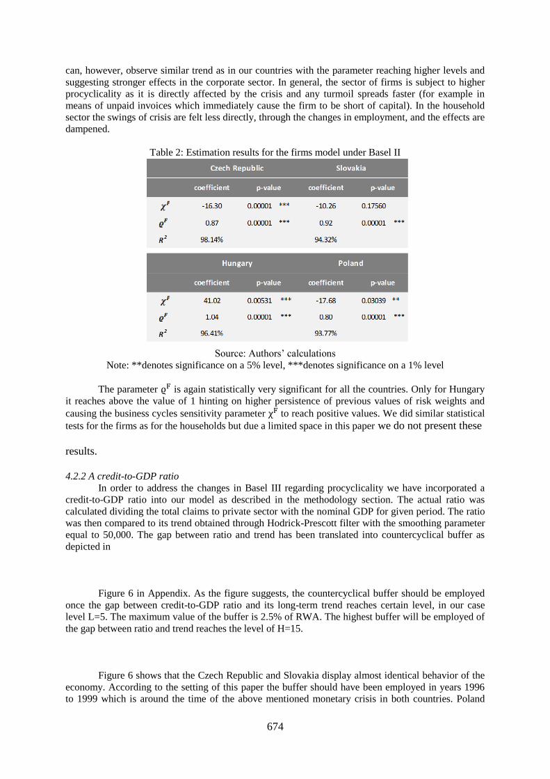
can, however, observe similar trend as in our countries with the parameter reaching higher levels and
suggesting stronger effects in the corporate sector. In general, the sector of firms is subject to higher
procyclicality as it is directly affected by the crisis and any turmoil spreads faster (for example in
means of unpaid invoices which immediately cause the firm to be short of capital). In the household
sector the swings of crisis are felt less directly, through the changes in employment, and the effects are
dampened.
Table 2: Estimation results for the firms model under Basel II
Source: Authors’ calculations
Note: **denotes significance on a 5% level, ***denotes significance on a 1% level
The parameter is again statistically very significant for all the countries. Only for Hungary
it reaches above the value of 1 hinting on higher persistence of previous values of risk weights and
causing the business cycles sensitivity parameter to reach positive values. We did similar statistical
tests for the firms as for the households but due a limited space in this paper we do not present these
results.
4.2.2 A credit-to-GDP ratio
In order to address the changes in Basel III regarding procyclicality we have incorporated a
credit-to-GDP ratio into our model as described in the methodology section. The actual ratio was
calculated dividing the total claims to private sector with the nominal GDP for given period. The ratio
was then compared to its trend obtained through Hodrick-Prescott filter with the smoothing parameter
equal to 50,000. The gap between ratio and trend has been translated into countercyclical buffer as
depicted in
Figure 6 in Appendix. As the figure suggests, the countercyclical buffer should be employed
once the gap between credit-to-GDP ratio and its long-term trend reaches certain level, in our case
level L=5. The maximum value of the buffer is 2.5% of RWA. The highest buffer will be employed of
the gap between ratio and trend reaches the level of H=15.
Figure 6 shows that the Czech Republic and Slovakia display almost identical behavior of the
economy. According to the setting of this paper the buffer should have been employed in years 1996
to 1999 which is around the time of the above mentioned monetary crisis in both countries. Poland

675
suggests a short period of buffer around the year 2000 while Hungary remains almost the whole
observed period of time buffer-less.
However, the most important and for all the four countries the same is the impulse to build
countercyclical buffer after 2006 when the ratio of credit to GDP started to rise significantly above its
long-term trend. This paper does not work with the potential use of the buffer as this does not directly
influence the risk weights. It is, however, to be assumed that such buffer would serve as a source of
capital in the critical years and smooth the procyclical effect of changes in capital adequacy.
4.2.3 Procyclicality of Basel III
Adding the countercyclical buffer to the capital requirements we have obtained time varying
capital requirements and a new set of risk weights. The comparison between Basel II and Basel III risk
weights for both households and firms is depicted in Figure 2. Under the settings of this paper the
countercyclical buffer would be imposed for both the Czech Republic and Slovakia in the second half
of 2006 when the credit growth exceeded the threshold given by the Credit-to-GDP ratio for both
households and firms. This would affect the risk weights for both sectors. Figure 2 demonstrates that
the risk weights decrease less after 2006 building a buffer and the amplitude is less pronounced.

676
Figure 2: Comparison of Basel II and Basel III risk weights for households and corporations (in %)
Source: Authors’ calculations

677
Hungary and Poland display the same effect for both sectors as the Czech Republic and
Slovakia but the imposition of the countercyclical buffer happens later, for Poland in the second half
of 2007 and for Hungary not until 2008. The new risk weights time series have been added to the
original regression equation to estimate the sensitivity of Basel III risk weights to the business cycle
(the complete results with Gretl outputs for Basel III are not enclosed but were done in a similar
manner as those for Basel II). Table 3 presents the estimation results for Basel III household model.
The estimation shows procyclicality for all countries except for Hungary, with reaching negative
values. However, the results are again not very statistically significant for Poland. In general the model
fits the data well with coefficient of determination over 75% for all countries. The inertia of
previous values of risk weights (defined by ) is similar to Basel II model, with for
Hungary switching the Hungarian business cycles sensitivity parameter into positive values.
Table 3: Estimation results for the households model under Basel III
Source: Authors’ calculations
Notes: *denotes significance on a 10% level, **denotes significance on a 5% level and ***denotes
significance on a 1% level
As to the assumptions of the model, tests have been again performed to ensure proper functionality of the regression model. Possible heteroskedasticity has been tested with the test of
White (1980) and the test could not reject the hypothesis of no heteroskedasticity present for any of
the countries. Based on other tests we also cannot reject the hypothesis of no collinearity. Normality of
residuals had to be rejected at first but control tests (Shapiro-Wilk (1965), Lilliefors (1967) and
Jarque-Bera (1987)) do not reject normality of residuals for Slovak households’ model. The
autocorrelation of disturbances has been tested with the Durbin-Watson statistics (Durbin & Watson
1951) showing values sufficiently close to 2 for Slovakia and Hungary. For Czech and Hungarian
households model possible autocorrelation has been further tested with the Breusch-Godfrey test for
autocorrelation (Breusch, 1979 and Godfrey, 1978) up to order 4 and the hypothesis of no
autocorrelation could also not be rejected. Table 4 proofs that transforming the model under Basel III
rules did not resolve the problem of Hungarian data and the results still do not correspond with the rest
of the region.
Figure 6 in Appendix depicts that adding the countercyclical buffer to the firms’ model we
obtain estimations of parameters.

678
Table 4: Estimation results for the firms model under Basel III
Source: Authors’ calculations
Notes: *denotes significance on a 10% level, **denotes significance on a 5% level and ***denotes
significance on a 1% level
With coefficient of determination around 95% for all countries the estimated model fits the
data very well. The estimates for parameter show again higher procyclicality of the firms sector
than the households sector due to reasons we have discussed with the Basel II results. The estimates
are statistically significant except for Slovakia where the p-value is significantly higher than 5%. The
parameter again suggests strong persistence of the risk weights, with Hungarian above 1. The
tests do not suggest presence of heteroskedasticity or collinearity. The Durbin-Watson statistics is
close to 2 for all countries except Poland where the possible autocorrelation has been tested with the
Breusch-Godfrey test up to order 4. The hypothesis of no autocorrelation cannot be rejected. The test
for normality of residuals has rejected normality of residuals for Czech Republic and Slovakia. After
performing additional tests the normality of residuals has not been rejected for Slovak firms under the
Lilliefors test. However, all tests have rejected the normality hypothesis for the Czech Republic.
4.2.4 Comparison of Basel II and Basel III results
Although Basel II and Basel III results are interesting on their own, for this paper the most
important is the comparison of the procyclicality under Basel III and Basel II (see
Figure 3 showing results for household sector). We have already proven that procyclicality
means negative correlation between the risk weights and the business cycle and therefore negative
values of the parameter . For households the procyclicality decreases with Basel III innovations
only for Slovakia. For Poland it stays around the same level while for the Czech Republic the results
display even higher procyclicality under Basel III for the households sector. When considering the
cyclicality in general (given by the absolute value of the parameter) we can see a decrease in
cyclicality even for Hungary.

679
Figure 3: Basel II and Basel III procyclicality for the household sector (as a % response to 1% change
in business cycle)
Source: Authors’ calculations
For the firms sector the results are more in favor of the original goal of Basel III, i.e. lower
procyclicality compared to Basel II (
Figure 4). The procyclicality is mitigated under the new framework for Czech and Slovak
firms while for Polish firms the level of sensitivity to business cycle stays again around the same. As
we already know from the previous section, Hungarian model does not correspond with the rest of the
region at all. But if we again take the cyclicality in absolute values, it will be decreased under Basel III
even for Hungarian firms.
Figure 4: Basel II and Basel III procyclicality for the firm sector (as a % response to 1% change in
business cycle)
Source: Authors’ calculations
The fact that the results for the firms sector show stronger mitigation of procyclicality speaks
also in favor of Basel III. As it was already mentioned, firms are the first sector to feel the swings of
business cycles. Recalling the amplitude of NPL or risk weights movements the firms sector oscillates
on much larger scale (Figure 5 in Appendix). Therefore, the mitigation of procyclicality for firms
might have more effect than mitigation for households where the sector is more stable and less elastic.
-6,00
-4,00
-2,00
0,00
2,00
4,00
6,00
8,00
10,00
Czech Republic Slovakia Hungary Poland
Basel II Basel III
-20,00
-10,00
0,00
10,00
20,00
30,00
40,00
Czech Republic Slovakia Hungary Poland
Basel II Basel III

680
5. Conclusion
The aim of this paper was to investigate the level of procyclicality under the two most recent
regulatory frameworks, Basel II and Basel III. The recent financial crisis has revealed many
shortcomings of the second Basel Accord and the amplification of the business cycle has been one of
them. When creating improved framework Basel III, the Basel Committee on Banking Supervision
sought to incorporate tools that would mitigate the procyclical nature of Basel II. Concentrating on the
countries of the Visegrád Group (the Czech Republic, Slovakia, Hungary and Poland) our aim was to
compare the procyclicality of both regulatory frameworks in the region and find out whether the
mitigating tools are effective. The exact hypotheses we sought to analyze supposed evident
procyclicality in Basel II (measured as negative correlation between the business cycle and Basel risk
weights) and decreased procyclicality in Basel III. We have also stipulated final hypothesis that the
countries of the region will react differently to the both Basel Accords as they have been differently
affected by the crisis.
Using the OLS estimation method we have analyzed separate models for households and
corporations under Basel II based on the stable capital adequacy ratio of 8%. For Basel III we have
incorporated the time varying countercyclical buffer into the model. The results of our estimation
immediately and clearly showed that we cannot reject the Hypothesis 3: different impact of Basel
Accords in the region. The results for Hungary differ greatly from the rest of the region as Hungary
has shown a completely different pattern in the input data. This is due to the fact that until recently the
Hungarians have obtained many loans in foreign exchange. Our data on non-performing loans was
therefore distorted by the foreign exchange development.
When refraining from Hungary, the expected procyclicality of Basel II has been confirmed by
our model and therefore Hypothesis 1 about procyclicality of Basel II could not be rejected. The
sensitivity to the business cycle has been higher for the firms than for the households, which is in line
with other studies analyzing Basel II. It is to be expected as the firms are the first ones to directly feel
the consequences of a crunch. The household sector is somewhat less elastic and the effects of a crisis
take longer to fully develop. Our model has, however, shown ambiguous results for Basel III,
mitigating the procyclicality for some sectors and countries while increasing it for others. Therefore
we have to reject the Hypothesis 2. If we would take into account Hungarian results as well we would
have to reject both Hypothesis 1 and Hypothesis 2 as the country displays no procyclicality at all.
However, all the countries report a strong persistence of the data as the risk weights are above all
dependent on its previous values. Such inertia has to be taken into account when considering any
change in the future regulatory rules.
The main contribution of this paper was the implementation of Basel III countercyclical tools
and of comparison between both frameworks. When applying a standard regulatory formula, we show
that results for Hungary differ greatly from the rest of the region as this country has shown a
completely different pattern in the input data. This conclusion that Basel III rules cannot be applied
generally for all countries should be appealing for both regulators and bankers. We believe that Basel
III will not prevent bank industry from another financial crisis and that Basel III will fail as both Basel
I and Basel II did.
References
ANGELINI, P. - ENRIA, A. - NERI, S. - PANETTA, F. - QUAGLIARIELLO, M. (2010):
Pro-cyclicality of capital regulation: is it a problem? How to fix it? Banca d'Italia Occasional
Papers, vol 4, pp. 1-45.
BCBS (2010a): Basel III. International Framework for Liquidity Risk Measurement,
Standards and Monitoring. Basel Committee on Banking Supervision. Available at
www.bis.org.
BCBS (2010b): Basel III: A Global Regulatory Framework for More Resilient Banks and
Banking Systems. Basel Committee on Banking Supervision. Available at www.bis.org.
BCBS (2010c): Guidance for national authorities operating the countercyclical capital buffer.
Basel Committee on Banking Supervision. Available at www.bis.org.

681
BREUSCH, T. S. (1979): Testing for Autocorrelation in Dynamic Linear Models. Australian
Economic Papers, vol. 17, pp. 334-355.
DURBIN, J. - WATSON, G. S. (1951): Testing for Serial Correlation in Least Squares
Regression, II. Biometrika, vol. 38, pp. 159-179.
GERALI, A. - NERI, S. - SESSA, L. - SIGNORETTI, F. M. (2009): Credit and Banking in a
DSGE Model of the Euro Area. Journal of Money, Credit and Banking, vol. 42, no. 6, pp.
107-141.
GODFREY, L. G. (1978): Testing Against General Autoregressive and Moving Average
Error Models when the Regressors Include Lagged Dependent Variables. Econometrica, vol.
46, pp. 1293-1302.
GORDY, M. B. - HOWELLS, B. (2004): Procyclicality in Basel II: Can We Treat the Disease
Without Killing the Patient? Journal of Financial Intermediation, vol. 15, pp. 395-417.
JARQUE, C. M. - BERA, A. K. (1987): A test for normality of observations and regression
residuals. International Statistical Review, vol. 55, no. 2, pp. 163-172.
KASHYAP, A. K., - STEIN, J. C. (2004): Cyclical Implications of the Basel II Capital
Standard. Federal Reserve Bank of Chicago Economic Perspectives, 1st Quarter, pp. 18-31.
LALL, R. (2009): Why Basel II Faile and Why Any Basel III is Doomed. GEG Working Paper
2009/52. Oxford: The Global Economic Governance Programme University Collage.
LILLIEFORS, H. (1967): On the Kolmogorov–Smirnov test for normality with mean and
variance unknown. Journal of the American Statistical Association, vol. 62, no. 318, pp. 399-
402.
REPULLO, R. - SAURINA, J. - TRUCHARTE, C. (2009): Mitigating the Procyclicality of
Basel II. CEPR Discussion Paper No. 7382, pp. 105-112.
SAURINA, J. (2009): Dynamic Provisioning: The experience of Spain. Crisis Response,
Public Policy for the Private Sector, no. 7, Washington DC: The World Bank.
SHAPIRO, S. S. - WILK, M. B. (1965): An analysis of variance test for normality (complete
samples). Biometrika, no. 52, vol. 3-4, pp. 591-611.
ŠOBOTNÍKOVÁ, P. (2011): Procyclicality in Basel II and Basel III, Master thesis, Institute
of Economic Studies, Faculty of Social Sciences, Prague: Charles University.
TEPLÝ, P. (2010): The Key Challenges of The New Bank Regulations. In Proceedings of
2010 International Conference on Business, Economics and Tourism Management. Paris:
World Academy of Science, Engineering and Technology, pp. 383-386.
VARSANYI, Z. (2007): Rating philosophies: some clarifications. MPRA Paper No. 1733.
Munich: MPRA.
WHITE, H. (1980). A Heteroskedasticity-Consistent Covariance Matrix Estimator and a
Direct Test for Heteroskedasticity. Econometrica, vol. 48, no. 4, pp. 817-838.

682
Appendix
Figure 5: Comparison of NPLs and GDP in the region from 4Q 2002 to 1Q 2010

683
Figure 6: Credit/GDP gap translated into countercyclical buffer (as % of RWA)

684
Table 5: Regression results for households in the Czech Republic (BASEL II risk weights)
Regression model:
Regression results:
Model 1:OLS. using observations 2003:1-2010:1 (T = 29)
Dependent variable: CZE_W_HH
Coefficient Std. Error t-ratio p-value
const 0.0679776 0.0258769 2.627 0.01426 **
CZE_CHANGE_lnY -0.473643 0.120165 -3.9416 0.00054 ***
CZE_LY_W_HH 0.88557 0.0654365 13.5333 <0.00001 ***
Mean dependent var 0.381399
S.D. dependent
var 0.066544
Sum squared resid 0.014674
S.E. of regression 0.023757
R-squared 0.88165
Adjusted R-
squared 0.872546
F(2. 26) 96.84373
P-value(F) 8.94e-13
Log-likelihood 68.89089
Akaike criterion -131.7818
Schwarz criterion -127.6799
Hannan-Quinn -130.4971
rho 0.307864 Durbin-Watson 1.126595
Testing the assumptions
White's test for heteroskedasticity
o Null hypothesis: Heteroskedasticity not present
o Test statistic: TR^2 = 14.412221, with p-value = P(Chi-square(5) > 14.412221) =
0.013192
Multicollinearity test
o Values > 10.0 may indicate a collinearity problem
o CZE_CHANGE_lnY 1.003
o CZE_LY_W_HH 1.003
Normality of residuals
o Null hypothesis: error is normally distributed
o Chi-square(2) = 3.052, with p-value 0.21740
Breusch-Godfrey Test for autocorrelation up to order 4
o Test statistic: LMF = 1.261266, with p-value = P(F(4,22) > 1.26127) = 0.315
o Alternative statistic: TR^2 = 5.409743, with p-value = P(Chi-square(4) > 5.40974) =
0.248
o Ljung-Box Q' = 6.63745, with p-value = P(Chi-square(4) > 6.63745) = 0.156

685
Table 6: Regression results for households in Hungary (BASEL II risk weights)
Regression model:
Regression results:
Model 5:OLS. using observations 2003:1-2010:1 (T = 29)
Dependent variable: HUN_W_HH
Coefficient Std. Error t-ratio p-value
const 0.0498862 0.0294981 1.6912 0.10276
HUN_CHANGE_lnY -1.02023 0.236756 -4.3092 0.00021 ***
HUN_LY_W_HH 1.10974 0.0460158 24.1166 <0.00001 ***
Mean dependent var 0.426903
S.D. dependent
var 0.300647
Sum squared resid 0.061007
S.E. of regression 0.04844
R-squared 0.975895
Adjusted R-
squared 0.974041
F(2. 26) 526.3097
P-value(F) 9.28e-22
Log-likelihood 48.2298
Akaike criterion -90.4596 Schwarz criterion -86.35771
Hannan-Quinn -89.17494
rho 0.229422 Durbin-Watson 1.431075
Testing the assumptions
White's test for heteroskedasticity
o Null hypothesis: Heteroskedasticity not present
o Test statistic: TR^2 = 10.722630, with p-value = P(Chi-square(5) > 10.722630) =
0.057165
Multicollinearity test
o Values > 10.0 may indicate a collinearity problem
o HUN_CHANGE_lnY 1.467
o HUN_LY_W_HH 1.467
Normality of residuals
o Null hypothesis: error is normally distributed
o Chi-square(2) = 1.697, with p-value 0.42796
Breusch-Godfrey test for autocorrelation up to order 4
o Test statistic: LMF = 1.485775, with p-value = P(F(4,22) > 1.48578) = 0.241
o Alternative statistic: TR^2 = 6.167888, with p-value = P(Chi-square(4) > 6.16789) =
0.187
Ljung-Box Q' = 8.30373, with p-value = P(Chi-square(4) > 8.30373) = 0.0811