process modelling and model analysis-hangos-cameron
TRANSCRIPT

8/17/2019 Process Modelling and Model Analysis-Hangos-Cameron
http://slidepdf.com/reader/full/process-modelling-and-model-analysis-hangos-cameron 1/560

8/17/2019 Process Modelling and Model Analysis-Hangos-Cameron
http://slidepdf.com/reader/full/process-modelling-and-model-analysis-hangos-cameron 2/560
PROCESS MODELLING
AND MODEL ANALYSIS

8/17/2019 Process Modelling and Model Analysis-Hangos-Cameron
http://slidepdf.com/reader/full/process-modelling-and-model-analysis-hangos-cameron 3/560
This is Volume 4 of
PROCESS SYSTEMS ENGINEERING
A Series edited by George Stephanopoulos and John Perkins
8/17/2019 Process Modelling and Model Analysis-Hangos-Cameron
http://slidepdf.com/reader/full/process-modelling-and-model-analysis-hangos-cameron 4/560
PROCESS
MODELLING AND
MODEL ANALYSIS
K. M. Hangos
Systems and Control Laboratory
Computer and Automation Research Institute of the
Hungarian A cademy of Sciences
Budapest, Hungary
L T. Cameron
Cape
Centre
Department of
Chemical Engineering
The U niversity of Queensland
Brisbane, Queensland
r^ ACADEMIC PRESS
\ , , _ _ ^ ^ A Harcourt Science and Technology Company
San Diego San Francisco New York Boston London Sydney Tokyo

8/17/2019 Process Modelling and Model Analysis-Hangos-Cameron
http://slidepdf.com/reader/full/process-modelling-and-model-analysis-hangos-cameron 5/560
This book is printed on acid-free paper.
Copyright © 2001 by ACADEMIC PRESS
All Rights Reserved.
No part of this publication may be reproduced or transmitted in any form or by any
means, electronic or mechanical, including photocopying, recording, or any
information storage and retrieval system , without the prior permission in writing from the
publisher.
Academic Press
A Harcourt Science and
Technology
Company
Harcourt Place, 32 Jamestown Road, London NW l 7BY, UK
http://www.academicpress.com
Academic Press
A H arcourt Science and
Technology
Company
525 B Street, Suite 1900, San Diego, California 92101-4495, USA
http ://w w w. academ icpress. com
ISBN 0-12-156931-4
Library of Congress Catalog Number: 00-112073
A catalogue record of this book is available from the British Library
Typeset by N ewgen Imaging Systems (P) Ltd., Chennai, India
01 02 03 04 05 06 BC 9 8 7 6 5 4 3 2 1
Transferred to digital printing in 2007.

8/17/2019 Process Modelling and Model Analysis-Hangos-Cameron
http://slidepdf.com/reader/full/process-modelling-and-model-analysis-hangos-cameron 6/560
Dedicated to
Misi, Akos, Veronika
and
Lucille, James, Peter, Andrew

8/17/2019 Process Modelling and Model Analysis-Hangos-Cameron
http://slidepdf.com/reader/full/process-modelling-and-model-analysis-hangos-cameron 7/560
This Page Intentionally Left Blank
8/17/2019 Process Modelling and Model Analysis-Hangos-Cameron
http://slidepdf.com/reader/full/process-modelling-and-model-analysis-hangos-cameron 8/560
CONTENTS
INTRODUCTION xiii
I F U N D A M E N T A L P R IN C IP L E S A N D PR O CE SS
M O D E L D E V E L O P M E N T
I T h e Role of Mo dels in Process
Systems Engineering
1.1. The Idea of a Mo del 4
1.2. Model App lication Areas in PSE 7
1.3. M odel Classification 10
1.4. M odel Charac teristics 12
1.5. A Brief Historical Review of M odelling in PSE 13
1.6. Sum mary 17
1.7. Review Ques tions 17
1.8. Ap plication Exercises 17
VII

8/17/2019 Process Modelling and Model Analysis-Hangos-Cameron
http://slidepdf.com/reader/full/process-modelling-and-model-analysis-hangos-cameron 9/560
VIII CONTENTS
2 A Systematic Approach to Model Building
2.1. The Process System and the M odelling Goal 20
2.2.
Mathematical Models 22
2.3.
A Systematic Modelling Procedure 24
2.4. Ingredients of Process Mo dels 32
2.5.
Summary 36
2.6. Review Questions 36
2.7.
Application Exercises 37
3 Conservation Principles
3.1. Thermo dynam ic Principles of Process Systems 42
3.2. Principle of Conservation 51
3.3.
Balance Volumes in Process System App lications 58
3.4. Summ ary 61
3.5.
Review Questions 62
3.6. Application Exercises 62
4 Constitutive Relations
4.1.
Transfer Rate Equations 65
4.2. Reaction Kinetics 70
4.3.
Thermodynamical Relations 72
4.4. Balance Volume Relations 75
4.5. Equipm ent and Control Relations 75
4.6.
Summary 79
4.7. Review Questions 79
4.8. Application Exercises 80
5 Dynamic Models—Lumped Parameter Systems
5.1. Characterizing Mo dels and Mo del Equation Sets 83
5.2. Lumped Parameter Models—Initial Value
Problems (IVPs) 84
5.3. Conservation Balances for Mass 86
5.4. Conservation Balance s for Energy 89
5.5. Conservation Balances for Mo mentum 95
5.6. The Set of Conservation Balances for Lum ped Systems 98
5.7. Conservation Balances in Intensive Variable Form 99
5.8. Dim ensionless Variables 101
5.9. Norm alization of Balance Equations 102
5.10. Steady-State Lum ped Parameter Systems 103
8/17/2019 Process Modelling and Model Analysis-Hangos-Cameron
http://slidepdf.com/reader/full/process-modelling-and-model-analysis-hangos-cameron 10/560
CONTENTS IX
5.11. Analysis of Lumped Parameter Models 104
5.12. Stability of the M athematical Problem 114
5.13. Summary 117
5.14. Review Que stions 118
5.15. App lication Exercises 118
6 Solution Strategies for
Lumped Parameter Mode ls
6.1.
Process Engineering Example Problems 124
6.2. Ordinary Differential Equations 125
6.3. Basic Concepts in Num erical Methods 126
6.4. Local Truncation Error and Stability 129
6.5. Stability of the Num erical Method 133
6.6. Key Num erical Methods 137
6.7. Differential-Algebraic Equation Solution Techniques 149
6.8. Summary 155
6.9. Review Que stions 156
6.10. App lication Exercises 156
7 Dynamic Models^—Distributed
Parameter Systems
7.1.
Development of DPS Mod els 163
7.2. Exam ples of Distributed Parameter M odelling 174
7.3.
Classification of DPS M odels 182
7.4. Lumped Parameter Models for Representing DPSs 185
7.5.
Summary 186
7.6. Review Que stions 187
7.7. App lication Exercises 187
8 Solution Strategies for Distributed
Parameter Models
8.1. Areas of Interest 191
8.2. Finite Difference M ethods 192
8.3.
Method of Lines 201
8.4. M ethod of Weighted Residuals 203
8.5. Orthogonal Collocation 206
8.6. Orthogonal Collocation for Partial Differential Equations 216
8.7. Summary 218
8.8. Review Questions 218
8.9. App lication Exercises 219
8/17/2019 Process Modelling and Model Analysis-Hangos-Cameron
http://slidepdf.com/reader/full/process-modelling-and-model-analysis-hangos-cameron 11/560
CONTENTS
9 Process Model Hierarchies
9.1. Hierarchy Driven by the Level of Detail 225
9.2. Hierarchy Driven by Characteristic Sizes 233
9.3. Hierarchy Driven by Characteristic Times 239
9.4. Summ ary 245
9.5.
Further Reading 246
9.6. Review Questions 246
9.7. Application Exercises 246
II A D V A N C E D P R OC ES S M O D E L L I N G A N D
M O D E L A N A L Y S I S
10 Basic Tools for Process M od el Analysis
10.1. Problem Statements and Solutions 251
10.2. Basic Notions in Systems and Control Theory 253
10.3.
Lumped Dynamic Mod els as Dynamic System Models 264
10.4. State Space Mo dels and Mo del Linearization 269
10.5. Structural Graphs of Lumped Dynamic Models 277
10.6. Summary 281
10.7.
Review Questions 281
10.8.
Application Exercises 282
11 D ata Acquisition and Analysis
11.1.
Sampling of Continuous Time Dynamic Models 286
11.2.
Data Screening 289
11.3.
Experiment Design for Parameter Estimation of
Static Mo dels 294
11.4. Experiment Design for Parameter Estimation of
Dynamic Models 295
11.5. Summary 296
11.6.
Further Reading 296
11.7. Review Questions 296
11.8. App lication Exercises 297
12 Statistical Model Calibration and Validation
12.1. Grey-Box Mo dels and Model Calibration 300
12.2.
Mod el Parameter and Structure Estimation 302
12.3.
Model Parameter Estimation for Static M odels 314
12.4. Identification: Model Parameter and Structure Estimation of
Dynamic Models 318
12.5.
CSTR : A Case Study of Model Parameter Estimation 323
12.6. Statistical Mo del Validation via Parameter Estimation 330

8/17/2019 Process Modelling and Model Analysis-Hangos-Cameron
http://slidepdf.com/reader/full/process-modelling-and-model-analysis-hangos-cameron 12/560
CONTENTS XI
12.7. Summary 331
12.8. Further Reading 331
12.9. Review Questions 331
12.10. App lication Exercises 332
13 Analysis of Dy na m ic Process Mo dels
13.1. Analysis of Basic Dyn amical Properties 336
13.2. An alysis of Structural Dynam ical Properties 341
13.3.
Mo del Simplification and Reduction 350
13.4. Summary 359
13.5. Further Reading 359
13.6. Review Questions 360
13.7.
App lication Exercises 361
14 Process Mo dell ing for C on tro l and
Diagnostic Purposes
14.1. Mod el-Based Process Control 364
14.2. Mod el-Based Process Diagnosis 370
14.3.
Qu alitative, Logical and AI Models 372
14.4. Summary 384
14.5. Further Reading 384
14.6. Review Questions 385
14.7.
Ap plication Exercises 385
15 Modell ing Discrete Event Systems
15.1.
Chara cteristics and Issues 388
15.2.
Approaches to Model Representation 388
15.3.
Solution of Discrete Event Dynamic System Mo dels 404
15.4. Analysis of Discrete Event Systems 408
15.5. Summary 410
15.6. Further Reading 411
15.7. Review Questions 412
15.8. Application Exercises 412
16 Modell ing Hybrid Systems
16.1.
Hybrid Systems Basics 415
16.2.
Approaches to Model Representation 420
16.3. Analysis of Hybrid Systems 430
16.4. Solution of Hybrid System Mo dels 431
16.5.
Summary 434
16.6. Further Reading 434

8/17/2019 Process Modelling and Model Analysis-Hangos-Cameron
http://slidepdf.com/reader/full/process-modelling-and-model-analysis-hangos-cameron 13/560
XII CONTENTS
16.7. Review Questions 435
16.8. Application Exercises 436
17 Mo delling App lications in Process Systems
17.1. Copper Converter Dynamics 438
17.2. Destruction of Phenol in Wastewater by
Photochem ical Reaction 445
17.3. Prefermenter System for Wastewater Treatment 451
17.4.
Granulation Circuit M odelling 456
17.5. Industrial Depro panizer using Structural Packing 462
17.6.
Summary 469
18 Computer Aided Process Modell ing
18.1. Introduction 472
18.2.
Industrial Dem ands on Com puter Aided M odelling Tools 472
18.3.
Basic Issues in CA PM Tools 474
18.4. Approaches to CAPM Tool Development 483
18.5.
Summary 492
19 Empirical Model Building
19.1.
Introduction 493
19.2. The M odelling Procedu re Revisited 494
19.3. Black-Box Modelling 497
19.4.
Traps and Pitfalls in Emp irical Mo del Building 511
19.5.
Summary 515
19.6. Further Reading 515
19.7.
Review Ques tions 516
19.8. Application Exercises 516
Appendix: Basic Mathem atic Tools 517
A. 1. Random Variables and Their Properties 517
A.2.
Hyp othesis Testing 521
A.3. Vector and Signal Norm s 522
A.4. Matrix and Operator Norms 523
A.5. Graphs 524
BIBLIOGRAPHY 527
INDEX 535
8/17/2019 Process Modelling and Model Analysis-Hangos-Cameron
http://slidepdf.com/reader/full/process-modelling-and-model-analysis-hangos-cameron 14/560
INTRODUCTION
Process modelling is one of the key activities in process systems engineering. Its
importance is reflected in various way s. It is a significant activity in m ost major com
panies around the world, driven by such application areas as process optimization,
design and control. It is a vital part of risk management, particularly consequence
analysis of hazardous events such as loss of containment of process fluids. It is a
permanent subject of conferences and symposia in fields related to process systems
engineering. It is often the topic of various specialized courses offered at graduate,
postgraduate and continuing professional education levels. There are various text
books available for courses in process modelling and model solution amongst which
are Himmelblau [1], Davis [2], Riggs [3] and Rice and Do [4]. These however are
mainly devoted to the solution techniques related to process models and not to the
problem on how to define, setup, analyse and test models. Several short monographs
or mathematical notes with deeper insights on modelling are available, most notably
by Aris [5] and Denn [6].
In most books on this subject there is a lack of a consistent modelling approach
applicable to process systems engineering as well as a recognition that modelling is
not just about producing a set of equations. There is far m ore to process m odelling
than writing equa tions. This is the reason w hy w e decided to write the current book in
order to give a more com prehensive treatmen t of process modelling useful to student,
researcher and industrial practitioner.
There is another important aspect which limits the scope of the present material
in the area of process modelling. It originates from the well-known fact that a par
ticular process model depends not only on the process to be described but also on the
modelling goal. It involves the intended use of the model and the user of that model.
Moreover, the actual form of the model is also determined by the education, skills
and taste of the modeller and that of the user. Due to the above reasons, the main
emphasis has been on process models for dynamic simulation and process control
purposes. These are principally lumped dynamic process models in the form of sets
of differential—algebraic equations. Other approaches such as distributed parameter
modelling and the description of discrete event and hybrid systems are also treated.
Finally the use of empirical mod elling is also covered, recogn izing that our knowledge
XIII
8/17/2019 Process Modelling and Model Analysis-Hangos-Cameron
http://slidepdf.com/reader/full/process-modelling-and-model-analysis-hangos-cameron 15/560
XIV INTRODUCTION
of many systems is extremely shallow and that input-output descriptions generated
by analysing plant data are needed to complement a mechanistic approach.
Process modelling is an engineering activity with a relatively mature technol
ogy. The basic principles in model building are based on other disciplines in process
engineering such as mathematics, chemistry and physics. Therefore, a good back
ground in these areas is essential for a modeller. Thermodynamics, unit operations,
reaction kinetics, catalysis, process flowsheeting and process control are the helpful
prerequisites for a course in process modelling. A mathematical background is also
helpful for the understanding and application of analysis and numerical methods in
the area of linear algebra, algebraic and differential equations.
Structure of the book
The book consists of two parts. The first part is devoted to the building of process
models whilst the second part is directed towards analysing models from the view
point of their intended use. The methodology is presented in a top-down systematic
way following the steps of a modelling procedure. This often starts from the most
general ca se. Emph asis is given in this book to identifying the key ingredients, devel
oping conservation and co nstitutive equations then analysing and solving the resultant
model. These concepts are introduced and discussed in separate chapters. Static and
dynam ic process m odels and their solution m ethods are treated in an integrated man
ner and then followed by a discussion on hierarchical process m odels which are related
by sc ales of time or degree of detail. This is the field of multi-scale mod elling.
The second part of the book is devoted to the problem of how to analyse process
mod els for a given modelling g oal. Three dominant app lication areas are discussed:
• control and diagnosis where mostly lumped dynam ic process models are used,
• static flowshee ting with lumped static process mod els,
• dynamic flowsh eeting where again mostly lumped dynamic process models
are in use.
Special emphasis is given to the different but related process models and their
properties which are important for the above application areas.
Various supplementary m aterial is available in the appendices. This inc ludes:
• Background m aterial from m athematics covering linear algebra and math
ematical statistics.
• Com puter science concep ts such as graphs and algorithms.
Each chapter has sections on review questions and application examples which
help reinforce the content of each chapter. Many of the application exercises are
suitable for group work by students.
The methods and procedures presented are illustrated by examples throughout
the book augmented with MATLAB subroutines where appropriate. The examples
are drawn from as wide a range of process engineering disciplines as possible. They
include chemical processing, minerals process engineering, environmental engineer
ing and food engineering in order to give a true process system's appeal. The model
analysis methods in part two are applied to many of the same process systems used
in part one. This method of presentation makes the book easy to use for both higher
year undergraduate, postgraduate courses or for self study.

8/17/2019 Process Modelling and Model Analysis-Hangos-Cameron
http://slidepdf.com/reader/full/process-modelling-and-model-analysis-hangos-cameron 16/560
INTRODUCTION
XV
Making use of the book
This book is intended for a wide audience. The authors are convinced that it will be
useful from the undergraduate to professional engineering level. The content of the
book has been presented to groups at all levels with adaptation of the material for
the particular audience. Because of the modular nature of the book, it is possible to
concentrate on a number of chapters depending on the need of the reader.
For the undergraduate, we suggest that a sensible approach will be to consider
Chapters 1-6, parts of 10-12 as a full 14-week semester course on basic process
modelling. For advanced modelling at undergraduate level and also for postgraduate
level. Chapters 7 -9 can be considered. Chapter 17 on Modelling Applications should
be viewed by all readers to see how the principles work out in practice.
Som e industrial professionals w ith a particular interest in certain application areas
could review modelling principles in the first half of the book before considering the
specific application and analysis areas covered by Chapters 11-19. The options are
illustrated in the following table:
Chapter
1. Role of Modelling in Process
Systems Engineering
2. A Modellling Methodology
3. Conservation Principles in
Process Modelling
4.
Constitutive Relations for
Modelling
5. Lumped Parameter Model
Development
6. Solution of Lumped Parameter
Models
7.
Distributed Parameter Model
Development
8. Solution of Distributed
Parameter Models
9. Incremental Modelling and
Model Hierarchies
10. Basic Tools for Model
Analysis
11. Data Acquisition and Analysis
12. Statistical Model Calibration
and Validation
13. Analysis of Dynamic Process
Models
14.
Process Modelling for Control
and Diagnosis
15.
Modelling of Discrete Event
Systems
16.
Modelling of Hybrid Systems
17. Modelling Applications
18.
Computer Aided Process
Modelling
19.
Empirical Model Building
Undergraduate
introduction
/
/
/
/
/
>r
/
/
/
/
Postgraduate
advanced
/
/
/
/
/
^
/
/
/
/
/
/
/
/
Professional
introduction
/
/
/
/
/
/
/
/
/
/
/
Professional
advanced
/
/
/
/
/
/
/
/
/
/
/
/
/

8/17/2019 Process Modelling and Model Analysis-Hangos-Cameron
http://slidepdf.com/reader/full/process-modelling-and-model-analysis-hangos-cameron 17/560
XVI INTRODUCTION
For instructors there is also access to PowerPoint presentations on all chapters
through
the
website: h t t p : / / d a i s y . c h e q u e . u q . e d u . a u / c a p e / m o d e l l i n g /
i n d e x . h t m l .
Acknowledgements
The authors are indebted to many people who co ntributed to the present book in
various ways. The lively atm osphere of the Department of Chemical Engineering of
The University of Queensland and the possibility for both of us to teach the final year
"Process Modelling and Solutions" course to several classes of chemical engineering
students has made the writing of the book possible. P resenting sections to professional
engineers within Australian industry and also to Ph.D. and academ ic staff in Europe
through
the
Eurecha organization,
has
helped refine some
of
the content.
We would especially thank Christine Smith for the care and help in prepar
ing different versions of the teaching materials and the manuscript. Also to Russell
Williams
and
Steven McGahey
for
help
in
reviewing some
of the
chapters
and to
Gabor Szederkenyi
for his
kind help w ith many
of
the LaTeX
and
figure issues.
We are conscious of the support of our colleagues working in the field of mod
elling in process systems engineering. These include Prof. John Perkins at Imperial
College, Prof. George Stephanopoulos at
MIT,
Professors R afique G ani and Sten Bay
Jorgensen at the Danish Technical University, Prof. Heinz Preisig at Eindhoven and
Prof. Wolfgang Marquardt at Aachen.
Special thanks
to Dr. Bob
Newell
for
many years
of
fruitful discussion
and
encouragement towards realism in modelling. We thank them all for the advice,
discussions and sources of material they have provided.
We readily acknowledge
the
contribution
of
many whose ideas
and
pub
lished works are evident in this book. Any omissions and mistakes are solely the
responsibility of the authors.

8/17/2019 Process Modelling and Model Analysis-Hangos-Cameron
http://slidepdf.com/reader/full/process-modelling-and-model-analysis-hangos-cameron 18/560
PARTI
FUNDAMENTAL PRINCIPLES
AND PROCESS MODEL
DEVELOPMENT

8/17/2019 Process Modelling and Model Analysis-Hangos-Cameron
http://slidepdf.com/reader/full/process-modelling-and-model-analysis-hangos-cameron 19/560
This Page Intentionally Left Blank

8/17/2019 Process Modelling and Model Analysis-Hangos-Cameron
http://slidepdf.com/reader/full/process-modelling-and-model-analysis-hangos-cameron 20/560
I
THE ROLE
OF
MODELS
IN
PROCESS SYSTEMS
ENGINEERING
M odels?— really nothing m ore than an imitation of reality We can relate to mo dels of
various types everywhere—some physical, others mathematical. They abound in all
areas of human activity, be it econ om ics, warfare, leisure, environment, c osmo logy or
engineering. Why such an interest in this activity of model building and model use?
It is clearly a means of gaining insight into the behaviour of systems, probing them,
controlling them, optimizing them. One thing is certain: this is not a new activity,
and some famous seventeenth-century prose makes it clear that some modelling was
considered rather ambitious:
From man or an gel the great Architect
Did wisely to conceal, and not divulge
His secrets to be scanned by them who ought
Rather adm ire; or if they list to try
Conjecture, he his fabric of the heavens
Hath left to their disputes, perhaps to move
His laughter at their quaint opinions wide
Hereafter, when they com e to m odel
heaven
And calculate the stars, how they will wield
The mighty frame, how
build, unbuild,
contrive
To save appearances, how gird the sphere
With ce ntric and eccentric scribbled o 'er.
Cycle and epicycle, orb in o rb,
[John Milton (1608-74), English poet. Paradise Lost, Book. 8: 72-84]
3

8/17/2019 Process Modelling and Model Analysis-Hangos-Cameron
http://slidepdf.com/reader/full/process-modelling-and-model-analysis-hangos-cameron 21/560
CHAPTER I THE ROLE OF MODELS IN PROCESS SYSTEMS ENGINEERING
Our task here is a little more modest, but nevertheless important for the field of
process engineering. In this chapter, we want to explore the breadth of model use in the
process industries—where models are used and how they are used. The list is almost
unlimited and the attempted modelling is driven largely by the availability of high
performance c ompu ting and the demands of an increasingly competitive marketplace.
However, we must admit that in many cases in process engineering much is
concealed by our limited understanding of the systems we seek to design or manage.
We can relate to the words of Milton that our efforts and opinions are sometimes
quaint and laughable and our conjectures short of the mark, but the effort may well
be worthwhile in terms of increased understanding and better management of the
systems we deal with.
The emphasis in this book is on mathematical modelling rather than physical
modelling, although the latter has an important place in process systems engineering
(PSE ) through small scale pilot plants to three dimensional (3D ) construction m odels.
I.I. THE IDEA OF A MODEL
A model is an imitation of reality and a mathematical model is a particular form of
representation. We should never forget this and get so distracted by the model that
we forget the real application which is driving the modelling. In the process of model
building we are translating our real world problem into an equivalent mathematical
problem which we solve and then attempt to interpret. We do this to gain insight
into the original real world situation or to use the model for control, optimization or
possibly safety studies.
In discussing the idea of a model, Aris [5] considers the well-known concept of
change of scale as being at the root of the word "model". Clearly, we can appreciate
this idea from the wealth of scale models, be it of process plant, toys or miniature
articles of real world items. However in the process engineering area the models we
deal with are fundamentally mathem atical in nature. They attempt to capture, in the
form of equations, certain characteristics of a system for a specific use of that m odel.
Hence, the concept of purpose is very much a key issue in model building.
The modelling enterprise links together a purpose
V
with a subject or physical
system <S and the system of equations
M
which represent the mod el. A series of
experiments £ can be applied to M in order to answer questions about the system S.
Clearly, in building a model, we require that certain characteristics of the actual
system be represented by the model. Those characteristics could include:
• the correct response direction of the outputs as the inputs chang e;
• valid structure which correctly represents the connection between the inputs,
outputs and internal variables;
• the correct short and/or long term behaviour of the model.
In some cases, certain characteristics which are unnecessary to the use of the
model are also included. The resultant model has a specific region of applicability,
depending on the experiments used to test the model beh aviour against reality. These
issues are more fully investigated in the following c hapters.
8/17/2019 Process Modelling and Model Analysis-Hangos-Cameron
http://slidepdf.com/reader/full/process-modelling-and-model-analysis-hangos-cameron 22/560
THE IDEA OF A MODEL
Real world
problem
A
1
Mathematical
problem
2
Mathematical
solution
3
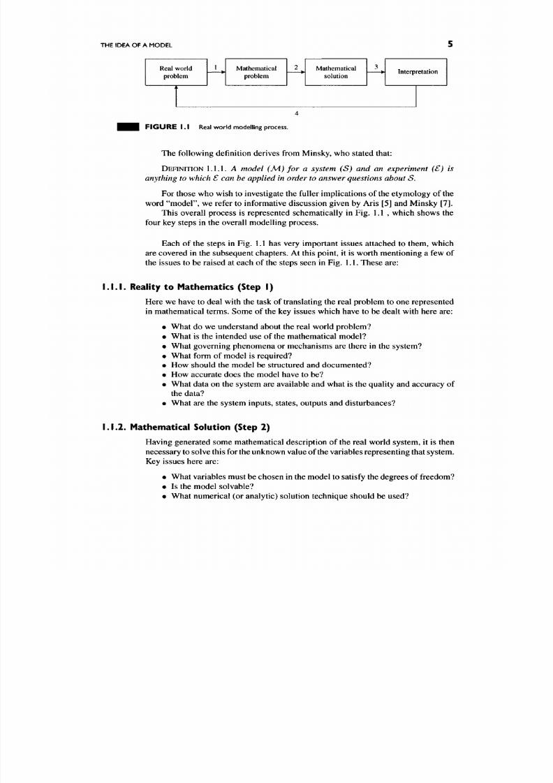
F I G U R E I . I Real wo rld modelling process.
The following definition derives from Minsky, who stated that:
DEFINITION 1.1.1. A model (M) for a system (S) and an experiment (£) is
anything to which £ can be applied in order to answer questions about S.
For those w ho wish to investigate the fuller implications of the etymo logy of the
word "model", we refer to informative discussion given by Aris [5] and Minsky [7].
This overall process is represented schematically in Fig. 1.1, which shows the
four key steps in the overall modelling process.
Each of the steps in Fig. 1.1 has very important issues attached to them, which
are covered in the subsequent chapters. At this point, it is worth mentioning a few of
the issues to be raised at each of the steps seen in Fig. 1.1. These are:
I.I.I. Reality to Mathematics (Step I)
Here we have to deal with the task of translating the real problem to one represented
in mathematical terms. Some of the key issues which have to be dealt with here are:
• What do we understand about the real world problem?
• W hat is the intended use of the mathem atical mode l?
• What governing phenomena or mechanisms are there in the system?
• Wh at form of model is required?
• How should the model be structured and documented?
• How accurate does the model have to be?
• W hat data on the system are available and what is the quality and accuracy of
the data?
• W hat are the system inputs, states, outputs and disturbances?
1. 1.2. Mathematical Solution (Step 2)
Having generated some mathematical description of the real world system, it is then
necessary to solve this for the unknown value of the variables representing that system.
Key issues here are:
• W hat variables must be chosen in the model to satisfy the degrees of freedom?
• Is the mod el solvable?
• Wh at num erical (or analytic) solution techniqu e should be used?
8/17/2019 Process Modelling and Model Analysis-Hangos-Cameron
http://slidepdf.com/reader/full/process-modelling-and-model-analysis-hangos-cameron 23/560
6 CHAPTER I THE ROLE OF MODELS IN PROCESS SYSTEMS ENG INEERING
• Can the structure of the problem be exploited to improve the solution speed or
robustness?
• What form of representation should be used to display the results (2D graphs,
3D visualization)?
• How sensitive will the solution output be to variations in the system parameters
or inputs?
I. L 3 . Interpreting the Model Outputs (Step 3)
Here we need to have procedures and tests to check whether our model has been
correctly im plemented and then ask w hether it imitates the real world to a sufficient
accuracy to do the intended
job.
Key issues include:
• How is the model implem entation to be verified?
• What type of model validation is appropriate and feasible for the problem?
• Is the resultan t model identifiable?
• What needs to be chang ed, added or deleted in the model as a result of the
validation?
• What level of simplification is justified?
• What data quality and quantity is necessary for validation and parameter
estimates?
• What level of model validation is necessary? Should it be static or dynamic?
• What level of accuracy is appropriate?
• What system parameters, inputs or disturbances, need to be known acc urately
to ensure model predictive quality?
L I .4 . Using the Results in the Real World (Step 4)
Here we are faced with the implementation of the model or its results back into the
real world problem we originally addressed. Some issues that arise are:
• For online applications wh ere speed might be essential, do I need to reduce
the model complexity?
• How can model updating be done and what data are needed to do it?
• Wh o will actually use the results and in what form should they ap pear?
• How is the model to be maintained?
• What level of docum entation is necessary?
These issues are just some of the many which arise as models are conc eptualized,
developed, solved, tested and implem ented. W hat is clear from the above discussion is
the fact that modelling
is ar more
than
simply
the
generation of a set of equations.
This
book emphasizes the need for a much broader view of process modelling including
the need for a model specification, a clear generation and statement of hypotheses
and assumptions, equation generation, subsequent model calibration, validation and
end use.
Many of the following chapters will deal directly with these issues. However,
before turning to those chapters w e should consider two m ore introductory aspects to
help "set the scene". These are to do with model characterization and classification.
The important point about stating these upfront is to be aware of these issues early
8/17/2019 Process Modelling and Model Analysis-Hangos-Cameron
http://slidepdf.com/reader/full/process-modelling-and-model-analysis-hangos-cameron 24/560
MODEL APPLICATION AREAS IN PSE
TA BL E I . I Mo de l Appl ica t ion Area s
Application area Mod el use and aim
Process design
Process control
Trouble-shooting
Process safety
Operator training
Environmental impact
Feasibility analysis of novel designs
Technical, econo mic, environmental assessment
Effects of process parameter changes on performance
Optimization using structural and parametric changes
Analysing process interactions
Waste minimization in design
Examining regulatory control strategies
Analysing dynamics for setpoint changes or disturbances
Optimal control strategies for batch operations
Optimal control for multi-product operations
Optimal startup and shutdown policies
Identifying likely causes for quality problems
Identifying likely causes for process deviations
Detection of hazardous operating regimes
Estimation of accidental release events
Estimation of effects from release scenarios (fire etc.)
Startup and shutdown for normal operations
Emergency response training
Routine operations training
Quantifying emission rates for a specific design
Dispersion predictions for air and water releases
Characterizing social and economic impact
Estimating acute accident effects (fire, explosion)
on and thus retain them as guiding concepts for what follows. Before we deal with
these issues, we survey briefly where m odels are principally used in PSE and w hat is
gained from their use.
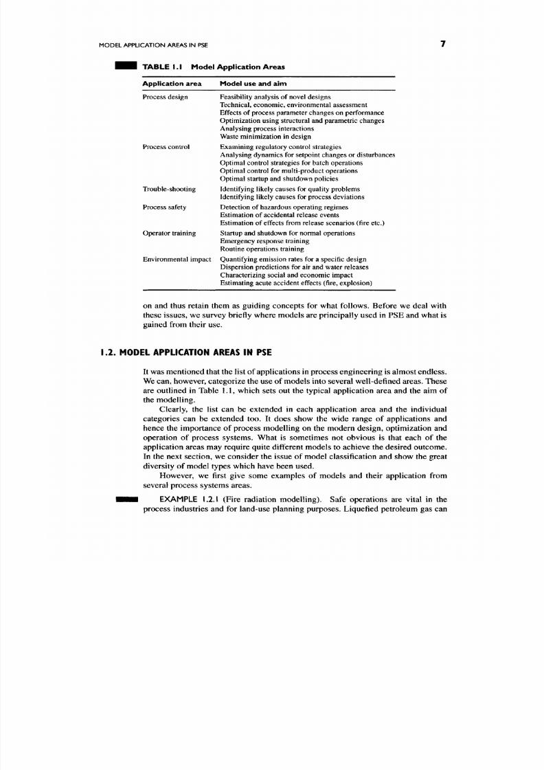
1.2. MODEL APPLICATION AREAS IN PSE
It was mentioned that the list of applications in process engineering is almost en dless.
We can , however, categorize the use of mod els into several well-defined areas. These
are outlined in Table 1.1, which sets out the typical application area and the aim of
the m odelling.
Clearly, the list can be extended in each application area and the individual
categories can be extended too. It does show the wide range of applications and
hence the importance of process modelling on the modern design, optimization and
operation of process systems. What is sometimes not obvious is that each of the
application areas may require quite different models to achieve the desired outcome.
In the next section, we consider the issue of model classification and show the great
diversity of model types which have been used.
However, we first give some examples of models and their application from
several process systems areas.
EXAMPLE 1.2.1 (F ire radiation mode lling ). Safe operations are vital in the
process industries and for land-use planning purposes. Liquefied petroleum gas can

8/17/2019 Process Modelling and Model Analysis-Hangos-Cameron
http://slidepdf.com/reader/full/process-modelling-and-model-analysis-hangos-cameron 25/560
CHAPTER I THE ROLE OF MODELS IN PROCESS SYSTEMS ENGINEERING
FIGURE 1 .2 BLEVE fireball caused by the rup ture o f an LPG tank (by permission of A.M . BIrk,
Queens University, Canada).
200 250 300 350
distance(metres)
FIGURE 1 .3 Radiation levels fo r
a
BLEVE incident.
500
be dangerous if released and ignited. O ne type of event which has occurred in several
places around the world is the boiling liquid expanding vapour explosion (BLEVE).
Figure 1.2 show s the form of a BLEV E fireball caused by the rupture of an LPG
tank. Of importance are radiation levels at key distances from the event as well as
projectiles from the rupture of the vessel.
Predictive mathematical mod els can be used to estimate the level of radiation at
nominated distances from the BLEVE, thus providing input to planning decisions.
Figure 1.3 shows predicted radiation levels (kW/m^) for a 50-tonne BLEVE out to a
distance of 500 m.
EXAMPLE 1.2.2 (Comp ressor dynamics and surge control). Com pressors are
subject to surge conditions when inappropriately controlled. When surge occurs, it

8/17/2019 Process Modelling and Model Analysis-Hangos-Cameron
http://slidepdf.com/reader/full/process-modelling-and-model-analysis-hangos-cameron 26/560
MOD EL A PPLICATION AREAS IN PSE
F I G U R E 1.4 Multi-stage centrifugal compressor (by permission of Mannesmann Demag Delaval).
12
10 I
0
Surge line
Shutdown
0 5 10 15 20 25
flow (kg/s)
F I G U R E 1.5 Head-flow dynamics during compressor shutdown.
30 35
can lead to serious dam age or destruction of the equipm ent. Effective co ntrol system s
are necessary to handle load changes. To test alternative control designs, accurate
mod elling and simulation are useful app roaches . Figure 1.4 show s a large multi-stage
compressor and Fig. 1.5 shows the predicted behaviour of the first stage head-flow
dynamics under controlled shutdown.
8/17/2019 Process Modelling and Model Analysis-Hangos-Cameron
http://slidepdf.com/reader/full/process-modelling-and-model-analysis-hangos-cameron 27/560
1 0 CHAPTER I THE ROLE OF MODELS IN PROCESS SYSTEMS ENG INEERING
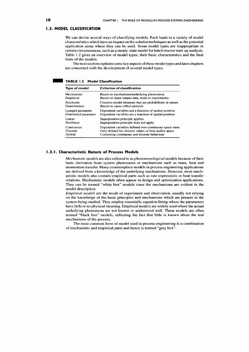
1.3. MODEL CLASSIFICATION
We can devise several ways of classifying models. Each leads to a variety of model
characteristics w hich have an impact on the solution techniques as well as the potential
application areas where they can be used. Some model types are inappropriate in
certain circum stances, such as a steady-state model for batch reactor start-up analysis.
Table 1.2 gives an overview of model types, their basic characteristics and the final
form of the models.
The next section explains som e key aspects of these model types and later chapters
are concerned with the development of several model types.
H H T A B L E 1.2 M o d e l C l as s if ic a ti on
Type of mo del Cr iter ion of classification
Mechanistic Based on mechanisms/underlying phenomena
Empirical Based on input-outpu t data, trials or experimen ts
Stochastic Contains mo del elem ents that are probabilistic in nature
Deterministic Based on cause -effect analysis
Lumped parameter Depen dent variables not a function of spatial position
Distributed parameter Depen dent variables are a function of spatial position
Linear Superposition principle applies
Nonlinea r Superposition principle doe s not apply
Continuous Dependent variables defined over continuous space-tim e
Discrete Only defined for discrete values of time and/or space
Hybrid Containing continuo us and discrete behaviour
1.3.1. Characteristic Nature of Process Models
Mechanistic models
are also referred to diS
phenomenological
models because of their
basic derivation from system phenomena or mechanisms such as mass, heat and
momentum transfer. Many commonplace models in process engineering applications
are derived from a knowledge of the underlying mechanisms. However, most mech
anistic models also contain empirical parts such as rate expressions or heat transfer
relations. Mechanistic models often appear in design and optimization applications.
They can be termed "white box" models since the mechanisms are evident in the
model description.
Empirical models are the result of experiment and observation, usually not relying
on the knowledge of the basic principles and mechanisms which are present in the
system being studied. They em ploy essentially equation fitting where the p arameters
have little or no physical mean ing. Em pirical models are widely used w here the actual
underlying phenomena are not known or understood well. These models are often
termed "black box" models, reflecting the fact that little is known about the real
mechanisms of the process.
The most common form of model used in process engineering is a combination
of mechanistic and empirical parts and hence is termed "grey box".
8/17/2019 Process Modelling and Model Analysis-Hangos-Cameron
http://slidepdf.com/reader/full/process-modelling-and-model-analysis-hangos-cameron 28/560
MODEL CLASSIFICATION I I
• • • EXAMPLE 1.3.1 (Empirical BLEV E Mo del). In Example 1.2.1 the radiation
levels from a BLEVE were illustrated. The size and duration of a BLEVE fireball
have been estimated from the analysis of many incidents, most notably the major
disaster in Mexico City during 1984. The empirical model is given by TNO [8] as
r = 3.24m^•^^^
t =
0.852m^'^^,
where r is fireball radius (m ),
m
the mass of fuel (k g) and
t
the duration of fireball (s).
• • •
Stochastic models arise when the description may contain elemen ts which have natural
random variations typically described by probability distributions. Th is characteristic
is often associated with phenomena which are not describable in terms of cause and
effect but rather by probab ilities or likeliho ods.
Deterministic models
are the final type of models characterized b y clear cause-effec t
relationships.
In most cases in process engineering the resultant model has elements from
several of these model classes. Thus we can have a mechanistic model with
some stochastic parts to it. A very common occurrence is a mechanistic model
which includes empirical aspects such as reaction rate expressions or heat transfer
relationships.
• • • EXAMPLE 1.3.2 (Mechanistic compressor mod el). Example 1.2.2 showed the
prediction of a compressor under rapidly controlled shutdown. The model used here
was derived from fundamental mass, energy and momentum balances over the com
pressor
plenum.
By assum ing ID axial flow the model was reduced to a set of ordinary
differential equations given by:
Mass: ——
= m\
—
m2\
at
dE
Energy: -— = m\h\
—
m2h2\
at
dM
Mom entum: — =
AmiPti
-Ptj)-^
^net
where
m\,m2
are inlet and outlet mass flows ,
h\,h2
the specific enthalpies , Am is the
inlet mean cross section, P/. are the inlet and outlet pressures and Fnet is net force on
• • • lumped gas volume.
Table 1.2 also includes other classifications dependent on assumptions about
spatial variations, the mathematical form and the nature of the underlying process
being m odelled.
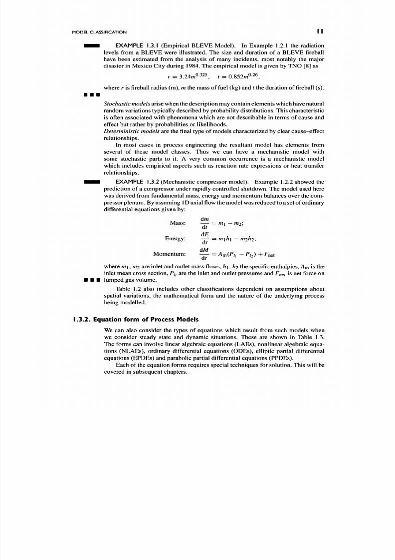
1.3.2. Equation form of Process Models
We can also consider the types of equations which result from such models when
we consider steady state and dynamic situations. These are shown in Table 1.3.
The forms can involve linear algebraic equations (LAEs), nonlinear algebraic equa
tions (NLAEs), ordinary differential equations (ODEs), elliptic partial differential
equations (EPDEs) and parabolic partial differential equations (PPDEs).
Each of the equation forms requires special techniques for solution. This will be
covered in subsequent chapters.
8/17/2019 Process Modelling and Model Analysis-Hangos-Cameron
http://slidepdf.com/reader/full/process-modelling-and-model-analysis-hangos-cameron 29/560
12
CHAPTER I THE ROLE OF MODELS IN PROCESS SYSTEMS ENGINEER ING
TABLE 1.3 Model Equation Form s
Type of model
Steady-state problem
Equation types
Dynamic problem
Deterministic
Stochastic
Lumped parameter
Distributed parameter
Linear
Nonlinear
Continuous
Discrete
Nonlinear algebraic
Algebraic/difference equations
Algebraic equations
EPDEs
Linear algebraic equations
Nonlinear algebraic equations
Algebraic equations
Difference equations
ODEs/PDEs
Stochastic ODEs or difference equations
ODEs
PPDEs
Linear ODEs
Nonlinear ODEs
ODEs
Difference equations
1.3.3.
Characteristics of the System Volumes
When we develop models, it is necessary to define regions in the system where we
apply conservation principles and basic physical and chem ical laws in order to derive
the mathematical description. These are the balance volumes. A basic classification
relates to the nature of the material in those volumes. Where there are both tem
poral and spatial variations in the properties of interest, such as concentration or
temperature, we call these systems "distributed". However, when there are no spa
tial variations and the material is homogeneous, we have a "lumped" system. The
complexity of distributed parameter systems can be significant both in terms of the
resulting model description and the required solution techniques. Lumped parameter
models generally lead to simpler equation systems which are easier to solve.
1.3.4.
Characteristics of the System Behaviour
When we consider system m odelling, there are many situations where discrete events
occur, such as turning on a pump or shutting a valve. These lead to discontinuous
behaviour in the system either at a known time or at a particular level of one of the
states such as temperature or concentration. T hese are called "tim e" or "state" events.
A model which has both characteristics is termed a hybrid system. These are very
common in process systems modelling.
Not only d o we need to consider the classification of the models that are used in
PSE applications but it is also helpful to look at some c haracteristics of those models.
1.4. MODEL CHARACTERISTICS
Here we consider some of the key characteristics which might affect our modelling
and analysis.
• M odels can be developed in hierarchies, where we can have several models for
different tasks or models with varying complexity in terms of their structure
and application area.
8/17/2019 Process Modelling and Model Analysis-Hangos-Cameron
http://slidepdf.com/reader/full/process-modelling-and-model-analysis-hangos-cameron 30/560
A BRIEF HISTORICAL REVIEW OF MOD ELLING IN PSE 1 3
• M odels exist with relative precision, which affect how and w here we can use
them.
• Mo dels cause us to think about our system and force us to consider the key
issues.
• Mo dels can help direct further experimen ts and in-depth investigations.
• Mo dels are developed at a cost in terms of money and effort. These need to be
considered in any application.
• Mo dels are always imperfect. It was once said by Georg e E. Box, a well-known
statistician, "All models are wrong, some are useful"
• M odels invariably require parame ter estimation of constants within the model
such as kinetic rate constants, heat transfer and mass transfer coefficients.
• M odels can often b e transferred from on e discipline to another.
• M odels should display the principle of parsimony, displaying the simplest
form to achieve the desired modelling goal.
• Mo dels should be identifiable in terms of their internal parameters.
• M odels may often need simplification, or model order reduction to become
useful tools.
• M odels may be difficult or impossible to adequately validate.
• M odels can become intractable in terms of their num erical solution.
We can keep some of these in mind when we come to develop models of our
own for a particular app lication. It is clearly not a trivial issue in some cases. In other
situations the model development can be straightforward.
1.5. A BRIEF HISTORICAL REVIEW OF MODELLING IN PSE
As a distinct discipline, PSE is a child of the broader field of systems engineering as
applied to processing operations. As such, its appearance as a recognized discipline
dates back to the m iddle of the twentieth century. In this section, w e trace briefly the
history of model building, analysis and model use in the field of PSE.
1.5.1.
The Industrial Revolution
It was the industrial revolution which gave the impetus to systematic approaches for
the analysis of processing and manufacturing operations. Those processes were no
longer simple tasks but became increasingly complex in nature as the demand for
commodity products increased. In particular, the early chemical developments of
the late eighteenth century spurred on by the Franco-British wars led to industrial
scale processes for the manufacture of gun powder, sulphuric acid, alkali as well
as food products such as sugar from sugar beet. In these developments the French
and the British competed in the development of new production processes, aided by
the introduction of steam power in the early 1800s which greatly increased potential
production capacity
In dealing with these new processes, it was necessary for the engineer to bring
to bear on the problem techniques derived from many of the physical sciences and
engineering disciplines. These analysis techniques quickly recognized the complex
interacting behaviour of many activities. These ranged from manufacturing processes
8/17/2019 Process Modelling and Model Analysis-Hangos-Cameron
http://slidepdf.com/reader/full/process-modelling-and-model-analysis-hangos-cameron 31/560
I 4 CHAPTER I THE ROLE OF MODELS IN PROCESS SYSTEMS ENGINEERING
to communication systems. The complexities varied enormously but the approaches
took on a "systems" view of the problem which gave due regard to the components
in the process, the inputs, outputs of the system and the complex interactions which
could occur due to the connected nature of the process.
Sporadic exam ples of the use of systems engineering as a sub-discipline of indus
trial engineering in the nineteenth and twentieth centuries found application in many
of the industrial processes developed in both Eu rope and the United S tates. This also
coincided with the emergence of chemical engineering as a distinct discipline at the
end of the nineteenth century and the development of the unit operations concept
which would dominate the view of chemical engineers for most of the twentieth cen
tury. There was a growing realization that significant benefits would be gained in
the overall economics and performance of processes when a systems approach was
adopted. This covered the design, control and operation of the process.
In order to achieve this goal, there was a growing trend to reduce complex
behaviour to simple mathematical forms for easier process design—hence the use of
mathematical models. The early handbooks of chemical engineering, e.g. Davis [9],
were dominated by the equipment aspects with simple models for steam, fluid flow
and mechanical behaviour of equipment. They were mainly descriptive in content,
emphasizing the role of the chemical engineer, as expressed by Davis, as one who
ensured:
. . . Com pleteness of reactions, fewness of repairs and econom y of hand labour
should be the creed of the Chemical Engineer.
Little existed in the area of process modelling aimed at reactor and separation
systems . In the period from 1900 to the mid-1920s there was a fast growing body
of literature on more detailed analysis of unit operations, which saw an increased
reliance on mathematical modelling. Heat exchang e, drying, evaporation, centrifuga-
tion, solids processing and separation technologies such as distillation were subject
to the application of mass and energy balances for model development. Many papers
appeared in such English journ als as
Industrial
&
Engineering C hemistry, Chemistry
and Industry,
and the
Society of the Chemical Industry.
Similar developments were
taking place in foreign langu age journ als, notably those in France and Germany. Text
books such as those by Walker and co-workers [10] at the Massachusetts Institute of
Technology, Olsen [11] and many monographs became increasingly analytic in their
content, this also being reflected in the education system.
1.5.2.
The Mid-twentieth Century
After the end of the Second World War there was a growing interest in the application
of systems engineering app roaches to industrial processes, especially in the chemical
industry. The mid-1950s saw many developments in the application of mathematical
modelling to process engineering unit operations, especially for the understanding
and prediction of the behaviour of individual units. This was especially true in the
area of chemical reactor analysis. Many prominent engineers, mathematicians and
scientists were involved. It was a period of applying rigorous mathematical analysis
to process systems which up until that time had not been analysed in such detail.

8/17/2019 Process Modelling and Model Analysis-Hangos-Cameron
http://slidepdf.com/reader/full/process-modelling-and-model-analysis-hangos-cameron 32/560
A BRIEF HISTORICAL REVIEW OF MOD ELLING IN PSE 1 5
However, the efforts were mainly restricted to specific unit operations and failed to
address the process as a "system".
This interest in mathematical analysis coincided with the early development and
growing availability of computers. This has been a major driving force in modelling
ever since. Some individuals, however, were more con cerned with the overall process
rather than the details of individual unit operations.
One of the earliest monographs on PSE appeared in 1961 as a result of work
within the Monsanto Chemical Company in the USA. This was authored by T.J.
Williams [12], who wrote:
. . . systems engineering has a significant co ntribution to make to the practice and
development of chemical engineering. The crossing of barriers between chemical
engineering and other engineering disc iplines and the use of advanced m athema tics
to study fundamental process mechanisms cannot help but be fruitful.
He co ntinued,
. . . the use of com puters and the developmen t of mathem atical process sim ulation
techniques may result in completely new method s and approaches wh ich will justify
themselves by economic and technological improvements.
It is interesting to note that Williams ' application of system s engineering c overed
all activities from proces s development through plant design to control and operation s.
Much of the work at Mo nsanto centred on the use of advanced control techn iques aided
by the development of computers capable of performing online control. Computer-
developed mathematical models were proposed as a basis for producing statistical
mod els generated from their more rigorous cou nterparts. The statistical models, which
were regression models, could then be used within a control scheme at relatively
low computational cost. It is evident that significant dependence was placed on the
development and use of mathematical models for the process units of the plant.
In concluding his remarks, Williams attempted to asses s the future role and impact
of systems engineering in the process industries. He saw the possibility of some 150
large-scale computers being used in the chemical process industries within the USA
for repeated plant optimization studies, these computers being directly connected to
the plant operation by the end of the 1960s. He wrote:
. . . the next 10 years, then, may see most of toda y's problem s in these fields
conquered.
He did, however, see some dangers not the least being
. . . the need for sympathetic persons in management and plant operations w ho
know and appreciate the power of the methods and devices involved, and who will
demand their use for study of their own particular plants.
1.5.3.
The Modern Era
Clearly, the vision of T.J. Williams was not met within the 1960s but tremendous
strides were made in the area of process modelling and simulation. The seminal

8/17/2019 Process Modelling and Model Analysis-Hangos-Cameron
http://slidepdf.com/reader/full/process-modelling-and-model-analysis-hangos-cameron 33/560
I 6
CHAPTER
I
THE ROLE OF MODELS IN PROCESS SYSTEMS ENGINEERING
work on transport phenomena by Bird et al. [13] in 1960 gave further impetus to the
mathematical m odelling of process system s through the use of fundamental principles
of conservation of mass, energy and mom entum. It has remained the pre-eminent book
on this subject for over 40 years.
The same period saw the emergence of numerous digital computer simulators
for both steady state and dynamic simulation. These were both industrially and aca
demically developed tools. Many of the systems were forerunners of the current
class of steady state and dynamic simulation packages. They were systems which
incorporated packaged models for many unit operations with little ability for the
user to model specific process operations not covered by the simulation system. The
numerical routines were crude by today's standards but simply reflected the stage of
development reached by numerical mathematics of the time. Efficiency and robustness
of solution were often poor and diagnostics as to what had happened were virtually
non-existent. Some things have not changed
The development of mini-computers in the 1970s and the emergence of UNIX-
based computers followed by the personal computer (PC) in the early 1980s gave a
boost to the development of modelling and simulation tools. It became a reality that
every engineer could have a simulation tool on the desk which could address a wide
range of steady state and dynamic simulation problems. This development was also
reflected in the process industries where equipm ent vendors w ere beginning to supply
sophisticated distributed control systems (DC Ss) based on mini- and microco mp uters.
These often incorporated simulation systems based on simple block representations of
the process or in some cases incorporated real time higher level compu ting langu ages
such as FORTRAN or BASIC. The system s were capable of incorporating large scale
real time optimization and supervisory functions.
In this sense, the vision of T.J. Williams some 40 years ago is a reality in cer
tain sectors of the process industries. Accompanying the development of the process
simulators was an attempt to provide computer aided modelling frameworks for the
generation of process models based on the application of fundamental conservation
principles related to mass, energy and momentum. These have been almost exclu
sively in the academic domain with a slowly growing penetration into the industrial
arena. Systems such as ASC END , Model.la, gPROMS or Modelica are among these
developments.
What continues to be of concern is the lack of com prehensive and reliable tools for
process mo delling and the almost exclusive slant towards the petrochem ical industries
of most commercial simulation systems. The effective and efficient development of
mathematical models for new and non-traditional processes still remains the biggest
hurdle to the exploitation of those models in PSE. The challenges voiced by T.J.
Williams in 1961 are still with us. This is especially the case in the non -petrochemical
sector such as minerals processing, food, agricultural products, pharmaceuticals,
wastewater and the integrated process and manufacturing industries where large scale
discrete-continuous operations are providing the current challenge.
Williams' final words in his 1961 volume are worth repeating,
. . . there are bright prospects ahead in the chemical process industries for systems
engineering.
One could add, . . . for the process industries in general and for modelling in
particular

8/17/2019 Process Modelling and Model Analysis-Hangos-Cameron
http://slidepdf.com/reader/full/process-modelling-and-model-analysis-hangos-cameron 34/560
APPL ICATION EXERCISES
1 7
1.6. SUMMARY
Mathematical models play a vital role in PSE. Nearly every area of application is
undergirded
by
some form
of
mathematical representation
of
the system behaviour.
The form
and
veracity
of
such models
is a key
issue
in
their
use.
Over
the
last
50
years, there
has
been
a
widespread
use of
models
for
predicting both steady state
and dynamic behaviour of processes. This was principally in the chemical process
industries
but,
more recently, these techniques have been applied into other areas
such as minerals, pharm aceuticals and bio-products. In most cases these have been
through
the
application
of
process simulators incorporating embedded models.
There is a maturity evident in traditional steady state simulators, less so in large
scale dynamic simu lators
and
little
of
real value
for
large scale discrete-con tinuous
simulation. Behind each of these areas there is the need for effective model d evelop
ment and doc umentation
of
the basis
for
the models which are developed. Systematic
approaches
are
essential
if
reliable m odel
use is to be
demanded.
The following chapters address
a
systematic approach to the mathematical devel
opment of process models and the analysis of those m odels. The idea that one m odel
serves
all
purposes
is
fallacious. Models must
be
developed
for a
specific purpose,
and that purpose w ill direct the mod elling task. It can be in any of the areas of model
application discussed
in
Section
1.2.
This point
is
emphasized
in
the following cha p
ter, which develops a systematic approach to model building. The rest of the book
provides d etailed information on underlying principles on which the m odels are built
and analysed.
1.7. REVIEW QUESTIONS
Q l . l . Wh at are the major steps in building a model of a process sy stem? (Section
1.1)
Q1.2.
What key issues might arise for each of the overall modelling steps?
(Section 1.1)
Q1.3. What major areas
of
PSE often rely
on the use of
models? What
are
some
of
the outcomes
in the use of
those models? (Section
1.2)
Q1.4.
How can mod els be classified into generic types? Are these categories m utually
exclusive?
If
not, then explain why. (Section
1.3.1)
Q1.5. Explain the fundamental differences between stoc hastic, empirical and mech
anistic mod els. What are som e of the factors which m ake it easier or harder to develop
such models? (Section 1.3.1)
Q1.6. What
are
some
of
the advantages
and
disadvantages
in
developing
and
using
empirical versus mechanistic models for process applications? (Section 1.3.1)
1.8. APPLICATION EXERCISES
A l . l . Consider the model application areas mentioned in Section 1.2. Give some
specific exam ples of models being used in those app lications? W hat w ere the benefits

8/17/2019 Process Modelling and Model Analysis-Hangos-Cameron
http://slidepdf.com/reader/full/process-modelling-and-model-analysis-hangos-cameron 35/560
I 8 CHAPTER I THE ROLE OF MODELS IN PROCESS SYSTEMS ENGINEERING
derived from developing and using models? Was there any clear methodology used
to develop the model for its intended purpose?
A1.2. Wh at could be the impedim ents to effective m odel building in process systems
applications? D iscuss these and their significance and possible w ays to overcome the
impediments.
A1.3. Consider a particular industry sector such as food, minerals, chem icals or
pharmac euticals and review w here and how mod els are used in those industry sec tors.
W hat forms of models are typically used? Is there any indication of the effort expended
in developing these m odels against the potential benefits to be derived from their use?
A1.4. Consider the basic principles of mass, heat and mom entum transfer and the
types of models which arise in these areas. What are the key characteristics of such
models describing, for example, heat radiation or heat conduction? How do you
classify them in terms of the classes mentioned in Table 1.3.
8/17/2019 Process Modelling and Model Analysis-Hangos-Cameron
http://slidepdf.com/reader/full/process-modelling-and-model-analysis-hangos-cameron 36/560

8/17/2019 Process Modelling and Model Analysis-Hangos-Cameron
http://slidepdf.com/reader/full/process-modelling-and-model-analysis-hangos-cameron 37/560
20
CHAPTER 2 A
SYSTEMATIC
APPROACH TO MODEL BUILDING
u
inputs
S
system
X
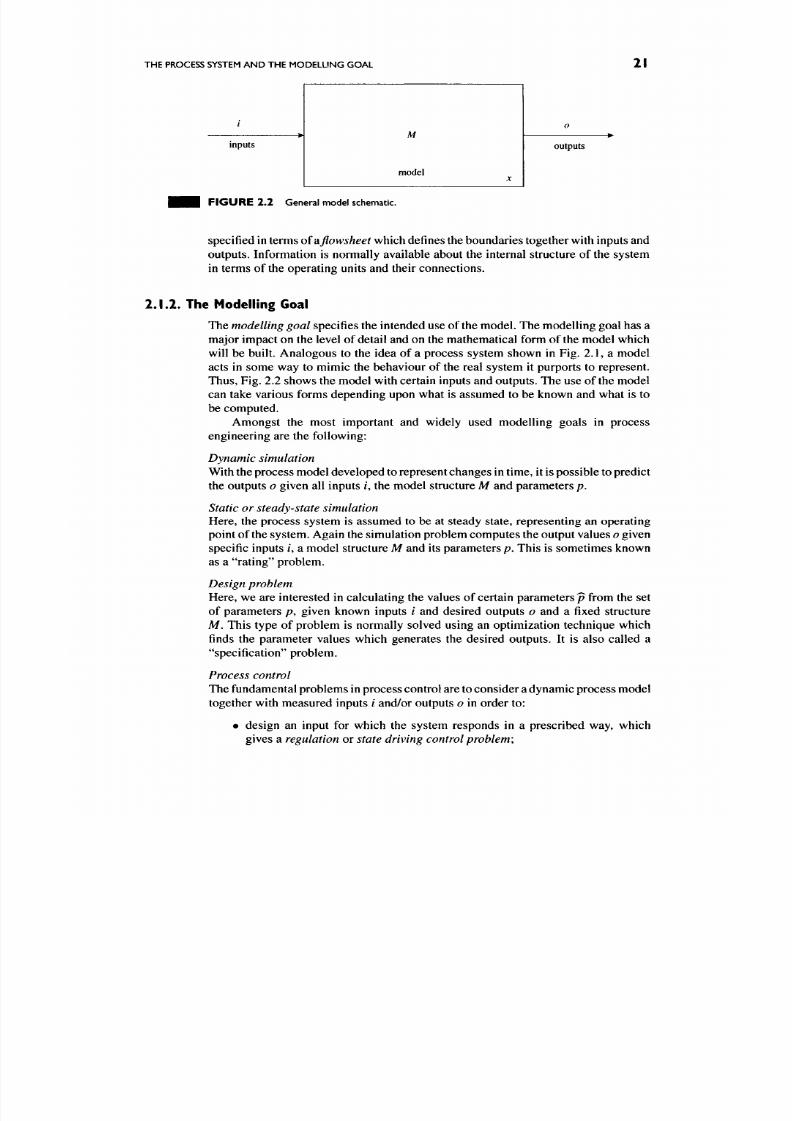
y
outputs
F I G U R E 2 . 1 General system schematic.
2 .1 .
THE PROCESS SYSTEM AND THE MODELLING GOAL
2 . 1 . 1 . The Notion of a Process System
If
we
want to understand the notion of
a
process system,
we can start from the general
notion of a
system.
This can be defined in an abstract sense in system theory. A
system is a part of the real world with well-defined physical bou ndaries. A system is
influenced by its surroundings or environm ent via its
inputs
and generates influences
on its surroundings by its
outputs
which occur through its boundary. This is seen in
Fig. 2.1.
We are usually interested in the behaviour of the system in time t eT.A system
is by nature a dynamic object. The system inputs u and the system outputs y can be
single valued, giving a single input, single output (SISO) system. Alternately, the
system can be a multiple input, multiple output (MIMO) system.
Both inputs and outputs are assumed to be time dependent possibly vector-valued
functions which we call signals.
A
system can b e viewed as an operator in abstract mathem atical sense transform
ing its inputs u to its outputs y . Th e states of the system are represented by the vector
X
and are usually associated with the mass, energy and m omentum holdups in the
system. N ote that the states are also signals, that is time-dependent functions. We can
express this mathematically as
M : T - > W C 7 ^ ^ J : T - > 3 ^ c 7 ^ ^ S:U-^y, y = S[u].
(2.1)
Here, the vector of inputs
M
is a function of time and this vector-valued signal is
taken from the set of all poss ible inpu ts
W
which are vector-valued signals of dimension
r.
The elements of the input vector at any given time r,
M/(0
can be integer, real or
symbolic values. Similarly, for the output vector}^ of dimension v.
The system S maps the inputs to the outputs as seen in Eq. (2 .1). Internal to the
system are the states
x
w hich allow a description of the behaviour at any point in time.
Moreover x{t) serves as a memory compressing all the past input-output history of
the system up to a given time
t.
A process system is then a system in which physical and chemical processes are
taking place, these being the m ain interest to the modeller.
The system to be modelled could be seen as the whole process plant, its envir
onmen t, part of
the
plant, an operating unit or an item of equipm ent. He nce, to define
our system we need to specify its boundaries, its inputs and outputs and the physico-
chemical processes taking place within
the
system. Process systems are co nventionally
8/17/2019 Process Modelling and Model Analysis-Hangos-Cameron
http://slidepdf.com/reader/full/process-modelling-and-model-analysis-hangos-cameron 38/560

8/17/2019 Process Modelling and Model Analysis-Hangos-Cameron
http://slidepdf.com/reader/full/process-modelling-and-model-analysis-hangos-cameron 39/560
22
CHAPTER
2 A
SYSTEMATIC APPROACH T O MODEL BUILDING
• find the structure of the model M with its parameters p using the input and
output data, thus giving a
system
identification
problem;
• find the internal states in M given a structure for the mod el, thus giving a state
estimation problem
which is typically solved using a form of least squares
solution;
• find faulty modes and/or system parameters which correspond to measured
input and output data, leading to fault detection and diagnosis problems.
In the second part of the book which deals with the analysis of process models,
separate chapters are devoted to process m odels satisfying different modelling go als:
Chapter 13 deals specifically with models for control. Chapter 15 with models for
discrete event systems, while Chapter 16 deals with models for hybrid or discrete-
continuous systems.
It follows from the above thai
a
problem definition in process modelling should
contain at least two sections:
• the specification of the process system to be modelled,
• the modelling goal.
The following exam ple gives a simple illustration of a problem definition.
wmm
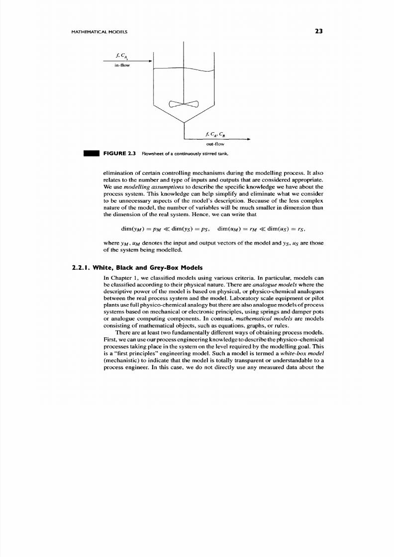
EXAMPLE 2.1.1 (Prob lem definition of a CS TR ).
Process system
Consider a continuous stirred tank reactor (CSTR) with continuous flow in and out
and with a single first-order chemical reaction taking place. The feed contains the
reactant in an inert fluid.
Let us assum e that the tank is adiabatic, such that its wall is perfectly insulated
from the surroundings. Th e flowsheet is shown in Fig. 2.3.
Modelling goal
Describe the dynamic behaviour of the CSTR if the inlet concentration changes. The
desired range of process variables will be between a lower value
x^
and an upper
• • • value x^ with a desired accuracy of 10%.
2.2. MATHEMATICAL MODELS
In Chapter 1, we discussed briefly some key aspects of models and, in particular,
mathematical models. We saw that models of various sorts are constructed and used
in engineering especially w here undertaking experim ents would not be possible, fea
sible or desirable for economic, safety or environmental reasons. A model can be
used to help design experiments which are costly or considered difficult or danger
ous. Therefore, a model should be similar to the real process system in terms of its
important properties for the intended use. In other words, the model should describe
or reflect somehow the properties of the real system relevant to the modelling go al.
On the other hand, models are never identical to the real process system. They
should be substantially less complex and hence much cheaper and easy to handle so
that the analysis can be carried out in a convenient way. The reduced complexity of
the model relative to the process system is usually achieved by simplification and
8/17/2019 Process Modelling and Model Analysis-Hangos-Cameron
http://slidepdf.com/reader/full/process-modelling-and-model-analysis-hangos-cameron 40/560
MATHEMATICAL MODELS
23
/ .C4
in-flow
O ^
out-flow
F I G U R E 2 . 3 Flowsheet of a continuously stirred tank.
elimination of certain controlling mechanisms during the modelling process. It also
relates to the number and type of inputs and outputs that are considered appropriate.
We use modelling assumptions to describe the specific knowledge we have about the
process system. This knowledge can help simplify and eliminate what we consider
to be unnecessary aspects of the model's description. Because of the less complex
nature of the model, the number of variables will be much smaller in dimension than
the dimension of the real system. Hence, we can write that
dim(jM) =PM
<^
dim(ys) = ps, dim(MM) = rM
< ^
dim(M5) = rs,
where yM, UM denotes the input and output vectors of the model and ys, us are those
of the system being modelled.
2.2.1.
White, Black and Grey-Box Models
In Chapter 1, we classified models using various criteria. In particular, models can
be classified ac cording to their physical nature. There are
analogue models
where the
descriptive power of the model is based on physical, or physico-chemical analogues
between the real process system and the model. Laboratory scale equipment or pilot
plants use full physico-ch emical analogy but there are also analogue mo dels of process
systems based on mechanical or electronic principles, using springs and damper pots
or analogue computing components. In contrast,
mathematical models
are models
consisting of mathematical objects, such as equations, graphs, or rules.
There are at least two fundamentally different ways of obtaining process mo dels.
First, we can use our process engineering know ledge to describe the physico-ch emical
processes taking place in the system on the level required by the modelling goa l. This
is a "first principles" engineering model. Such a model is termed a
white-box model
(mechanistic) to indicate that the model is totally transparent or understandable to a
process engineer. In this case, we do not directly use any measured data about the
8/17/2019 Process Modelling and Model Analysis-Hangos-Cameron
http://slidepdf.com/reader/full/process-modelling-and-model-analysis-hangos-cameron 41/560
24 CHAPTER 2 A SYSTEMATIC APPROACH
TO
MODEL BUILDING
proces s. However, we do make use of measured data indirectly, through the form and
the value of the system parameters.
Second, the alternative mean s of obtaining process m odels is often dictated by a
lack of accumulated engineering knowledge of the system. In this case, we can use
measurement data of the inputs and outputs to build a process model. The need to
stimulate or excite the system to obtain useful information for model identification
is a major issue for any model builder. This includes the amount of data and its
frequency content which enables the key responses to be captured in the resulting
mo del. In this case, we can use structure and parameter estimation methods developed
mainly in the field of process identification. This kind of m odel is called a black-box
model (empirical) because knowledge of the process is only available through the
measurement data and not from the underlying mechanisms. A good coverage of
system identification methods is given by Ljung [14]
In process engineering practice, however, both purely white and purely black-
box models are rare. In most cases, we use a suitable combination of our
a priori
process engineering knowledge to determine the structure and some of the parameter
values of the model. We then use measured data to build the model. This involves
the definition of kinetic and transport mechanisms, the estimation of key kinetic
and transport parameters as well as validation of the model against the performance
specifications. These combination models are termed
grey-box models.
The terms used in this section are m ore recent inventions; however, the underlying
principles and practice have existed for decades.
2.3. A SYSTEMATIC MODELLING PROCEDURE
Like other engineering tasks, good practice requires models to be constructed fol
lowing a well defined sequence of steps. These steps are arranged in a "Seven (7)
Step Modelling Procedure" which is introduced below and shown schematically in
Fig. 2.4.
However, it should be noted that m odel developm ent is inherently iterative in its
nature. One m ust usually return to and repeat an earlier step in case of any prob lems,
unusual or unwanted developm ents later in the process. No one gets it right irst ime
In fact, w e never get a perfect m odel, just one that is usable.
Before starting to setup
a
process model
the
problem definition should
be
clearly
stated.
This defines the process^ the modelling goal and the validation criteria.
This
is part of the formal description in the
SEVEN STEP MODELLING PROCEDURE,
which
is given in the form of an algorithmic problem. An algorithm being a systematic
procedure for carrying out the modelling task, nam ed after the Persian mathem atician
Abu Ja'far Mohammed ibn Musa al Khowarizm of the ninth century [15].
In a formal d escription of an algorithmic problem, one should formally specify
the following items:
• the inputs to the problem in the Given section,
• the desired output of the procedure in the
Find
or
Compute
section,
• the method description in the Procedure or Solution section.
Problem statements and their use in analysing computational or algorithmic
complexity will be described later in Section 10.1 in Chapter 10.
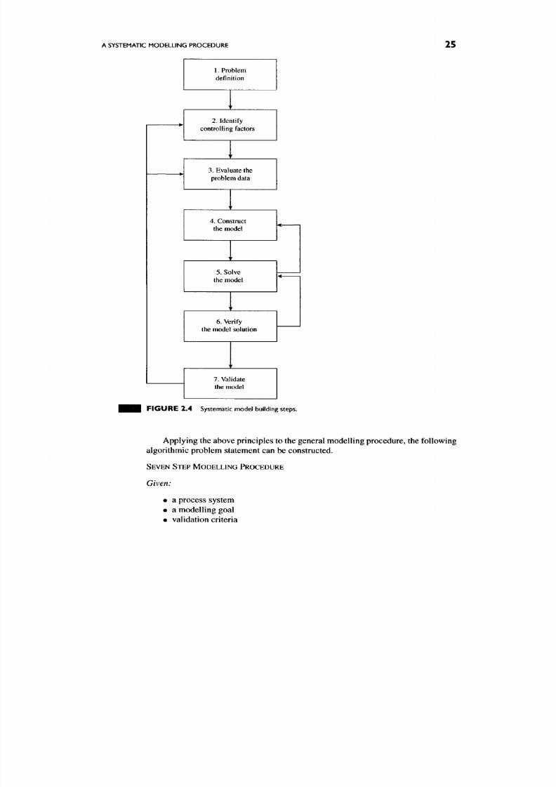
8/17/2019 Process Modelling and Model Analysis-Hangos-Cameron
http://slidepdf.com/reader/full/process-modelling-and-model-analysis-hangos-cameron 42/560
A SYSTEMATIC MODELLING PROCEDURE
25
1.
Problem
definition
T
2.
Identify
controlling factors
T
3.
Evaluate the
problem data
^
4. Construct
the model
^
5. Solve
the model
' r
6. Verify
the model solution
'
r
7. Validate
them odel
F I G U R E 2 . 4 Systematic model building steps.
Applying the above principles to the general modelling procedure, the following
algorithmic problem statement can be constructed.
SEVEN STEP MODELLING PROCEDURE
Given:
• a process system
• a mod elling goal
• validation criteria
8/17/2019 Process Modelling and Model Analysis-Hangos-Cameron
http://slidepdf.com/reader/full/process-modelling-and-model-analysis-hangos-cameron 43/560
26 CHAPTER 2 A SYSTEMATIC APPROACH
TO
MODEL BUILDING
Find:
•
a mathematical model
Procedure:
The model is built following a systematic procedure given below with seven steps.
The steps of the modelling procedure are as follows:
1.
Define the problem
This step refines the sec tions already present in the problem definition: the description
of the process system with the mod elling goal. M oreover, it fixes the degree of detail
relevant to the modelling goal and specifies:
• inputs and outputs
• hierarchy level relevant to the model or hierarchy levels of the model in the
case of hierarchical mod els (see Chapter 9 for hierarchy levels)
• the type of spatial distribution (distributed or lumped m odel)
• the necessary range and accuracy of the model and
• the time characteristics (static versus dynamic) of the process mo del.
2.
Identify the controlling factors or mechanisms
The next step is to investigate the physico-chemical p rocesses and phen omen a taking
place in the system relevant to the modelling goal. These are termed controlling
factors or mechanisms.
The most important and common controlling factors include:
• chemical reaction
• diffusion of ma ss
• conduction of heat
• forced convec tion heat transfer
• free convection heat transfer
• radiation heat transfer
• evaporation
• turbulent mixing
• heat or mass transfer through a boundary layer
• fluid flow
Figure 2.5 shows schematically the situation which exists when attempting to model
a process system . As we consider the system under study, we recognize the following
issues:
• There is a set of all proc ess charac teristics which are never fully identified.
• In the set of all process characteristics for the system w e often:
- only identify and include in the model a subset of the essential characteris
tics. This means that some essential characteristics for the application can
be missing from our model description;
- include non-essential characteristics of the system in our mo dels, which
lead to unnecessary complexity and/or model order (or size).
• We sometimes incorrectly identify process characteristics which are actually
not part of the system and include them in our model.
The previous issues are often difficult to resolve and very dependent on our
understanding of the system and our insight into what is important. Model validation
and the principle of parsimony, which seeks the simplest representation for the task
are the tools that need to be em ployed to address these issues.
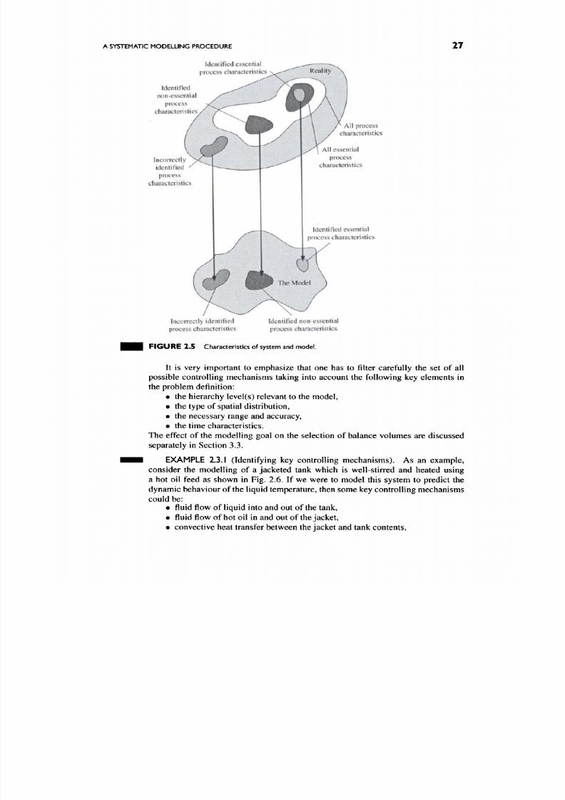
8/17/2019 Process Modelling and Model Analysis-Hangos-Cameron
http://slidepdf.com/reader/full/process-modelling-and-model-analysis-hangos-cameron 44/560
A SYSTEMATIC MODELLING PROCEDURE
27
Identified essential
process characteristics
Identified
non-essential
process
characteristics
Incorrectly
identified
process
characteristics
' All process
characteristics
All essential
process
characteristics
Identified essential
process characteristics
Incorrectly identified
process characteristics
Identified n on-essential
process characteristics
F I G U R E 2 . 5 Characteristics of
system
and model.
It is very important to emphasize that one has to filter carefully the set of all
possible controlling mechanisms taking into account the following key elements in
the problem definition:
• the hierarchy level(s) relevant to the model,
• the type of spatial distribution,
• the necessary range and accuracy,
• the time charac teristics.
The effect of the modelling goal on the selection of balance volumes are discussed
separately in Section 3.3.
EXAMPLE 2.3.1 (Identifying key controlling mecha nism s). As an exam ple,
consider the modelling of a jacketed tank which is well-stirred and heated using
a hot oil feed as shown in Fig. 2.6. If we were to model this system to predict the
dynamic behaviour of the liquid temperature, then some key controlling mechanisms
could be:
• fluid flow of liquid into and out of the tank,
• fluid flow of hot oil in and out of the jacket,
• convective heat transfer between the jacke t and tank contents.

8/17/2019 Process Modelling and Model Analysis-Hangos-Cameron
http://slidepdf.com/reader/full/process-modelling-and-model-analysis-hangos-cameron 45/560
28
CHAPTER 2 A SYSTEMATIC APPROACH TO MODEL BUILDING
Cold feed in
Hot oil in
Hot oil out
Heated liquid out
FIGURE 2.6 Heated tank.
• work input done through the agitator,
• convective heat losses from the jack et to the environment,
• convective heat losses from the surface of the heated liquid to the environm ent,
• evaporative losses of liquid from the tank contents to the environm ent.
We would need to assess the mo st important or essential characteristics required
in the model for
the
stated m odelling goal. This initially requires an order of magnitude
assessment
of
mass and heat transfer rates
to
see what is
of
major importanc e.
The models for these controlling factors are developed in physical chemistry,
reaction engineering, mass and heat transfer and unit operations. They form partial
models within the overall process m odel. Th ese partial models are generally black
box in their nature.
3.
Evaluate the data for the problem
As
it has
been already noted, mod els
of
real process systems
are of
the grey-box
type, therefore, we almost always need to use either measured process data directly
or estimated parameter values in our mod els.
It is very important to consider both m easured process data and parameter val
ues together with their uncertainties
or
precision.
Some default precision values
might be:
• industrial measured data is ± 1 0 to 30% ,
• estimated parameters from laboratory or pilot-p lant data is
±5
to 20%,
• reaction kinetic data is ± 1 0 to 500% ,
if nothing else
is
specified.
At this step, we may find out that there are neither suitable param eter values
found in the literature nor measured data to estimate them. This situation may force
us to reconsider our decisions in steps 1 and 2 and to return there to ch ange them.
4.
Develop
a
set of model equa tions
The model equations in a process model are either differential (both partial and
ordinary differential equations may appear) or algebraic equations. The differential
8/17/2019 Process Modelling and Model Analysis-Hangos-Cameron
http://slidepdf.com/reader/full/process-modelling-and-model-analysis-hangos-cameron 46/560
A SYSTEMATIC MODELLING PROCEDURE 29
equations
originate from conservation balanc es; therefore they can be termed
balance
equations. The algebraic equations are usually of mixed origin: they will be called
constitutive equations.
Conservation balances are discussed in detail in Chapter 3,
while constitutive equations are treated in Chapter 4.
A
model building sub-procedure
can be used to obtain a syntactically and
semantically correct process model. The steps and properties of this sub-procedure
are found in a separate Section 2.3.1 below.
5. Find and implement a solution procedure
Having set up a mathem atical mod el, we must identify its mathem atical form and find
or implement a solution p rocedu re. In all cases , we must ensure that the model is well
posed such that the "excess" variables or degrees of freedom are satisfied. We also
try and avoid certain numerical problems such as high index systems at this stage.
Lack of solution techniqu es may prevent a modeller using a particular type of process
model and can lead to additional simplifying assum ptions to obtain a solvable model.
This can be the case with distributed parameter process models.
6.
Verify
the model solution
Having a solution
is
just the start of the analysis. Verification is determining whether
the model is behaving correctly. Is it coded correctly and giving you the answer
you intended? This is not the same as model validation where we check the model
against reality. You need to check carefully that the model is correctly implem ented.
Structured programming using "top-down" algorithm design can help here as well
as the use of modular code which has been tested thoroughly. This is particularly
important for large-scale models.
7. Validate the model
Once a mathematical m odel has been set up, one should try to validate it. This checks
the quality of the resultant model against independent observations or assumptions.
Usually, only partial validation is carried out in practical cases depending on the
modelling goal.
There are various possibilities to validate a process model. The actual valida
tion method strongly depends on the process system, on the modelling goal and on
the possibilities of getting independent information for validation. The possibilities
include but are not limited to:
• verify experimentally the simplifying assum ptions,
• com pare the model behaviour with the process behaviour,
• develop analytical mod els for simplified cases and compare the behaviour,
• compare with other models using a common problem,
• com pare the model directly with process data.
The too ls to help carry out this task include the use of sensitivity studies to identify the
key controlling inpu ts or system param eters as well as the use of statistical validation
tests.
These can involve hypothesis testing and the use of various measures such as
averages, variances, maxima, minima and correlations.
If the validation results show that the developed model is not suitable for the
modelling goal then one has to return to step 2 and perform the sequence again.
Usually, validation resu lts indicate how to imp rove the mo del. We can often identify
the inadequate areas in our model development and, therefore, not all modelling
efforts are lost. No te that the final model is impossible to obtain in one pass through
the modelling procedure. Some iterations should be expected.
8/17/2019 Process Modelling and Model Analysis-Hangos-Cameron
http://slidepdf.com/reader/full/process-modelling-and-model-analysis-hangos-cameron 47/560
30
CHAPTER
2 A
SYSTEMATIC APPROACH TO MODEL BUILDING
A separate chapter in the second part of the book is devoted to model validation,
see Chapter 12.
2 . 3 . 1 . The Model Building Sub-procedure
Step 4 in the above SEVEN STEP MODELING PROCEDURE is a compos ite step in itself. It
is broken down to sub-steps which are to be carried out sequentially but with inherent
loops. The steps of this sub-procedure are as follows:
Mode l building sub-procedure in step 4,
4.0. System and subsystem boundary and balance volume definitions
The ou tcome of this step is the set of balance volum es for mass, energy and m omentum
leading to the conserved extensive quantities normally considered in process system s,
such as total system mass, component masses or energy.
In order to define the balanc e volumes we need to identify within our system the
regions where ma ss, energy or mom entum are likely to accumu late. These are termed
the system "holdups". The accumulation of conserved quantities such as energy or
mass are often dictated by the physical equipment or phase behaviour within that
equipment.
The following simple example of the heated tank illustrates the balance volume
identification problem.
• • • EXAMPLE 2.3.2 (Defining balance volumes). In Fig. 2.6, the example of a
liquid heating system was given. What could be the relevant balance volumes to
consider for this situation? One possibility is shown in Fig. 2.7, which gives two
main balance volumes:
E j ' : which is the balance volume (1) for mass (M ) and energy {E)
related to the liquid being heated;
which is the balance volui
related to the heating o il.
Other options are also possible depending on the characteristics of the system.
Ti2
' : which is the balance volume (2) for mass (M) and energy (£")
4.1. Define the characterizing variables
Here, we need
to
define the variables which w ill characterize the system being studied.
These v ariables are associated w ith the inputs, outputs and internal states of the system
as shown in
Fig. 2.1.
The variable we use will be strongly determined by our m odelling
goals. For the inputs and outputs w e can consider comp onent flows, total flow, mass or
molar concentrations. Temperatures and pressures may also be important, depending
on whether energy is considered important. For the internal states of the system,
the characterizing variables are related to the variables representing the main mass,
energy and mom entum holdups.
4.2.
Establish the balance equations
Here, we set up conservation balances for mass, energy and momentum for each
balance volume.

8/17/2019 Process Modelling and Model Analysis-Hangos-Cameron
http://slidepdf.com/reader/full/process-modelling-and-model-analysis-hangos-cameron 48/560
A SYSTEMATIC MODELLING PROCEDURE
31
Cold feed in
Hot oil in
> Heated liquid out
F I G U R E 2 . 7 Balance volumes fo r heated tank.
4.3. Transfer rate specifications
The rate expressions for transfer of heat, mass and momentum between different
balance volum es in the conservation b alances are specified here, usually as functions
of intensive quantities, such as concentrations and temperature.
4.4.
Prope rty relation specifications
These are mostly algebraic relationships expressing thermodynamic knowledge
such as equations of state and the dependence of physico-chemical properties on
thermodynamic state variables such as pressure, temperature and composition.
4.5. Balance volume relation specifications
An equipment with a fixed physical volume is often divided into several balance
volumes if multiple phases are present. A balance volume relation describes the
relationship between balance volumes and physical volumes.
4.6.
Equipment and control constraint specifications
There is inevitably the need to define constraints on process systems. These are typi
cally in the form of equipment operating constraints (for the pressures, temperatures
etc.) and in terms of control constraints, which define relations between manipulated
and controlled variables in the system.
4.7.
Modelling assumptions
When developing a particular model we apply modelling assumptions to get our
model equations. These assumptions form an integral part of the resultant model.
Therefore, they are regarded as ingredients of a process model together with the
model equations, their initial and boundary conditions. The ingredients of a process
model will be discussed in more detail in the Section 2.4.
It is impo rtant to note that
modelling assum ptions are usually built up incremen
tally
in
parallel a nd during sub-steps
4.0.-4.6,
8/17/2019 Process Modelling and Model Analysis-Hangos-Cameron
http://slidepdf.com/reader/full/process-modelling-and-model-analysis-hangos-cameron 49/560
32
CHAPTER
2 A
SYSTEMATIC APPROACH TO MODEL BUILDING
2.3 .2 .
Incremental Model Building
As it has been emphasized already in Section
2.3.1,
the steps of the m odel building
sub-procedure
should be carried out in a sequential-iterative manner. It means that
the model equations are built up incrementally repeating sub-steps
4.2.-4.7.
in the
following order of conserved extensive qu antities:
1.
Overall mass sub-model
The conservation balanc es for the overall mass in each of the balance volumes
and the variables therein appear in all other conservation balance s. Th erefore,
this subset of model equation is built up first performing sub-steps
4.2.-4.7.
of the model building sub-procedure.
2.
Com ponent mass sub-model
With the conservation balances for the overall mass in each of the balance
volumes given, it is easy to set up the conservation b alances for the com ponent
masses. This sub-set of model equation is added to the equations originated
from the overall mass balances performing sub-steps 4.2.^.7.
of
the
model
building sub-procedure.
3.
Energy sub-model
Finally, the subset of model equations induced by the energy balance is added
to the equations performing sub-steps 4.2.-4.7.
of the model building sub-
procedure.
This way the kernel of the the mod el building sub-procedure is repeated at least
three times for every balance volumes.
2.4. INGREDIENTS OF PROCESS MODELS
The SEVEN STEP MODELLING PROCEDURE described above shows that a process model
resulting from this procedure is not simply a set of equations. It incorporates a lot more
information. In order to encourage the clarity of presentation and the consistency of
the process model, a
structural presentation
incorporating all key ingredients is now
suggested.
1. Assumptions—which include but are not limited to
• time characteristics
• spatial characteristics
• flow conditions
• controlling mec hanisms or factors
• neglected depen dencies, such as
- temperature dependenc e of physico-chem ical properties
- concentration dependen ce of physico-chem ical properties
• required range of states and associated accuracy.
Here, we are careful to designate each assumption with a unique identifier
Ai, i =
1, 2 , . . . , n, where n is the total number of modelling assumptions.
2.
M odel equations and characterizing variables
Here , we have differential (balance) equations for
• overall mass, component masses for all components for all phases in all
equipment at all hierarchical levels (where applicable).
8/17/2019 Process Modelling and Model Analysis-Hangos-Cameron
http://slidepdf.com/reader/full/process-modelling-and-model-analysis-hangos-cameron 50/560
INGREDIENTS OF PROCESS MODELS
33
• energy (or enthalpy ),
• momentum;
constitutive equations for
• transfer rates: mass transfer, h eat/energy transfer, and reaction rates ,
•
property relations:
thermodynamical constraints and relations, such as the
depen dence of thermodynam ical properties on the thermody namical state vari
ables (temperature, pressu re and com positions), equilibrium relations and state
equations,
•
balance volume relations:
relationships between the defined mass and energy
balance regions,
• equipm ent and control cons traints;
and the variables which characterize the system:
• flows, temperatures, pressures, concentrations, enthalpies,
• mass, energy and mom entum holdups.
3.
Initial conditions
(where applicable)
Initial cond itions are needed for the differential (balance) equa tions in dynam ic pro
cess models. Initial conditions for all algebraic variables are also important since most
solutions are numerical.
4. Boundary conditions
(where applicable)
Boundary conditions must be specified for the differential (balance) equations in
spatially distributed process models.
5. Parameters
As a result of step 3 in the SEVEN STEP MODELLING PROCEDURE the value and/or
source of the model param eters are specified here with their units and precision. Th is
also applies to all variables in the model.
We can return to our earlier Exam ple 2.1.1 to illustrate how these ing redients are
to be expressed.
I H I H EXAMPLE 2.4.1 (Modelling example: CST R). Develop a process model of
the continuously stirred tank specified in Example 2.1.1 for dynamic prediction and
control purposes following the SEVEN STEP MODELLING PROCEDURE with all of its
ingredients.
1. Problem definition
The process system to be modelled is a continuously stirred tank with continuous
fluid flow in and out and with a single first order chemical reaction
A -^ B
taking
place in an inert solvent. The tank is adiabatic with its wall perfectly insulated from
the environment. The flowsheet schematic of this tank is shown in the Fig. 2.3.
(This description of
the
process system is exactly the same as the
Process system
section in the Problem definition of Example 2.1.1.)
The
modelling goal
is to predict the behaviour of the principal mass and energy
states of the tank contents if the inlet concentration is changed o ver a stated range. The
accuracy of the predictions should be ±10% of the real process. (It is again identical
to the Modelling goal section of the Problem definition.)
2. Controlling factors or mechanisms
• chem ical reaction
• perfect mixing
8/17/2019 Process Modelling and Model Analysis-Hangos-Cameron
http://slidepdf.com/reader/full/process-modelling-and-model-analysis-hangos-cameron 51/560
34 CHAPTER 2 A SYSTEMATIC APPROACH
TO
MODEL BUILDING
3. D ata for the problem
No m easured data is specified; therefore, w e use the following parameter type data:
• reaction kinetic data, heat of reaction
• physico-chemical properties
• equipment parameters
from the literature or given by the process documentation.
4.
Process model
Assumptions
A\\ perfect mixing,
A2'.
constant physico-chemical properties
^43: equal inflow and outflow (implying constant liquid volume with V =
constant),
A^\ single first-order exothermic reaction, A —>• P,
^ 5 :
adiabatic operation.
Model equ ations and characterizing variables
Differential (balance) equations in molar units
^ = / A i - / A - rV , (2.2)
at
^P'^P^
=fCpMT\ - 7-) + rV (- A //R ). (2.3)
Constitutive equations
r = ko.-'n^^'CA.
mA = CAV,
fA i
= / Q i .
fA =fCA^
Variables
t
CA
V
f
CA,
r
Cp
^Pi
T
Ti
A//R
E
ko
R
P
time [s]
concentration in the tank [mol/m^]
liquid volume [m^]
volumetric flowrate [m ^/s]
inlet concentration [mol/m-^]
reaction rate [mol/(sm^)]
specific heat of mixture [ J/(mol K)]
specific heat of feed / [J/(mol K)]
temperature in the tank [K]
inlet temperature [K]
heat of reaction [J/mol]
activation energy [J/mol]
pre-exponential factor [s~^]
universal gas constant, 8.314 [J/(mol K)]
density of mixture [mol/m^]
(2.4)
(2.5)
(2.6)
(2.7)

8/17/2019 Process Modelling and Model Analysis-Hangos-Cameron
http://slidepdf.com/reader/full/process-modelling-and-model-analysis-hangos-cameron 52/560
INGREDIENTS OF PROCESS MODELS 35
Pi
density of feed / [mol/m^]
niA moles of A [mol]
/ i j inlet flowrate of species A [mol/s]
Initial conditions
Boundary conditions
None
Parameters
Values for the following parameters with 10% precision:
V" , / , C A J , Ti, Cp, Cp., p, Pi
and for the reaction parameters with 30% precision:
^0, E,
A / / R
5. Solution procedure
Solve using an OD E or differential-algebraic equation solver.
6. Model verification
Implement model equations using structured programming principles. Check code
for correct execution. Check output trends against expected trends for reactor given
step changes in feed variables. Also, check predicted steady-state values after a feed
disturbance.
7. Model validation
Provide measured data from pilot plant or real process. Analyse plant data quality.
Carry out validation of predicted outpu ts from step test of system using least squ ares
estimation of error. Apply hypo thesis testing to validate model based on least squ ares
• • estimates. Refine model as required by performance criteria.
2.4.1.
Incremental Evolution of the Ingredients of Process Models
As it is described in Section 2.3.2 above, the ingredients of a process model are set
up incrementally in the following order:
• overall mass sub-mod el
• component mass sub-model
• energy sub-model
for every balance volume in the system.

8/17/2019 Process Modelling and Model Analysis-Hangos-Cameron
http://slidepdf.com/reader/full/process-modelling-and-model-analysis-hangos-cameron 53/560
3 6
CHAPTER
2 A
SYSTEMATIC APPROACH TO MODEL BUILDING
This implies that the following ingredients are subject to incremental evolution:
• assumptions,
• model equations and characterizing variables including differential (balance)
equations and constitutive equations,
• initial and boundary conditions,
• parameters.
The following example illustrates how this is done for the CSTR reactor ex ample
of Example 2.4.1.
• • • EXAMPLE 2.4.2 (Incremental evolution of the ingredients of a CSTR model).
Show the incremental evolution of the process mo del of the continuously stirred tank
modelled in Example
2.4.1.
The following evaluation steps are carried out.
1. List general modelling assumptions
These are assum ptions derived from the problem statement valid for the whole process
system. In this case, these are assumptions A\ and ^2 -
2.
Overall mass balances
There is an assumption on equal in- and outflow in the problem statement formalized
as assumption A3 which implies constant volumetric and mass holdup. Therefore,
the mass balance reduces to the equation V = constant.
3. Component mass balances
The relevant assumptions derived from the problem statement are assumptions A4
and ^ 5 . With these assumptions, w e set up the component mass balance equation
(2.2) with its constitutive equations (2.4)-(2.7).
4.
Energy balances
• • • Finally, the energy balance Eq. (2.3) is added.
2.5. SUMMARY
In this chapter, we have discussed a systematic m odel building strategy. The strategy
has been laid down in seven steps which are closely interrelated. As well, we noted
that the process is cyclic requiring the m odeller to retrace steps higher in the strategy
when the modelling, solution or validation are unacceptable. Also, the importance
of identifying key underlying mechanisms is emphasized in determining what is of
importance in the modelling task. These often need to be revisited to confirm how
significant their inclusion or exclusion might be.
It is vitally important that the model is both verified and validated. Various
approaches were discussed. Later chapters will take up these issues in more detail.
In the following chapter, we introduce the basic underlying process and
thermodynamic principles on which the model equations are based.
2.6. REVIEW QUESTIONS
Q2.1. Describe the general characteristics of a system. What is important to consider
in engineering systems? (Section 2.1)

8/17/2019 Process Modelling and Model Analysis-Hangos-Cameron
http://slidepdf.com/reader/full/process-modelling-and-model-analysis-hangos-cameron 54/560
APPLICATION EXERCISES
37
Q2.2.
Desc ribe typical mod elling goals for a range of proce ss engineering applica
tions.
(Section 2.1)
Q2.3. Discu ss why modelling assum ptions are important in the building of a mo del.
(Section 2.2)
Q2.4.
What is the difference betw een white, black- and grey-box m odels? (Section
2.2)
Q2.5.
Outline the systematic approach to model building discussed in this chapter.
What are the key steps and their characteristics? (Section 2.3)
Q2.6. Wh at are some controlling factors or mec hanism s which might be considered
in a process modelling task? (Section 2.3)
Q2.7. In defining the modelling problem, what basic decisions need to be made
before any mathematical modelling starts? (Section 2.3)
Q2.8.
In developing the mathem atical form of the model, what are the key equation
sub-classes to be considered? (Section 2.3)
Q2.9. Wh at technique s will help in model verification? (Section 2.3)
Q2.10.
Discus s some general approaches to model validation. (Section 2.3)
Q2.11, List the five necessary ingredients that go to make up a full m odel of a process
system (Section 2.4)
2.7 .
APPLICATION EXERCISES
A2.1. Con sider the following tank problem w here liquid is pump ed into an open
tank and then flows out under gravity. The situation is shown in Fig. 2.8.
If this situation is to be modelled for analysis of disturbance s in the inlet flow pres
sure from the pum p, develop the problem specification by considering the ingredients
needed for the model.
^
• x ^
• X I -
F I G U R E 2 . 8 Simple tank and liquid flow system.
A2.2. Con sider now a similar situation to that described in application A2.1, where
now the tank is enclosed. This is shown in Fig. 2.9. Again develop a problem
specification outlining all the ingredients for the mo delling.

8/17/2019 Process Modelling and Model Analysis-Hangos-Cameron
http://slidepdf.com/reader/full/process-modelling-and-model-analysis-hangos-cameron 55/560
38
CHAPTER 2 A SYSTEMATIC APPROACH TO MODEL BUILDING
^
->lx^
-CXF—>
F I G U R E 2 . 9 Enclosed tank.
A2.3. Consider a vessel (Figure 2.10), where a liquid feed is heated. Vapour and
liquid are withdrawn. It is intended that a model of this process should be developed
to investigate changes in the heat input
Q
from the steam coil as well as changes in
feed conditions of temperature and composition. Develop a problem description for
this situation discussing the necessary ingredients for the modelling.
vapour
feed
- steam
l iquid
F I G U R E 2 . 1 0 Liquid heating system.
A2.4. Consider Fig.
2.11,
which shows
a
packed absorber for
the
removal of a so lvent
within an air stream. The vessel is packed w ith activated carbon particles held in place
by screens. Develop a problem description, outlining the principal ingredients for
modelling which considers the system response to changes in the incoming solvent
concentration.
F I G U R E 2 . 1 1 Packed bed absorber.
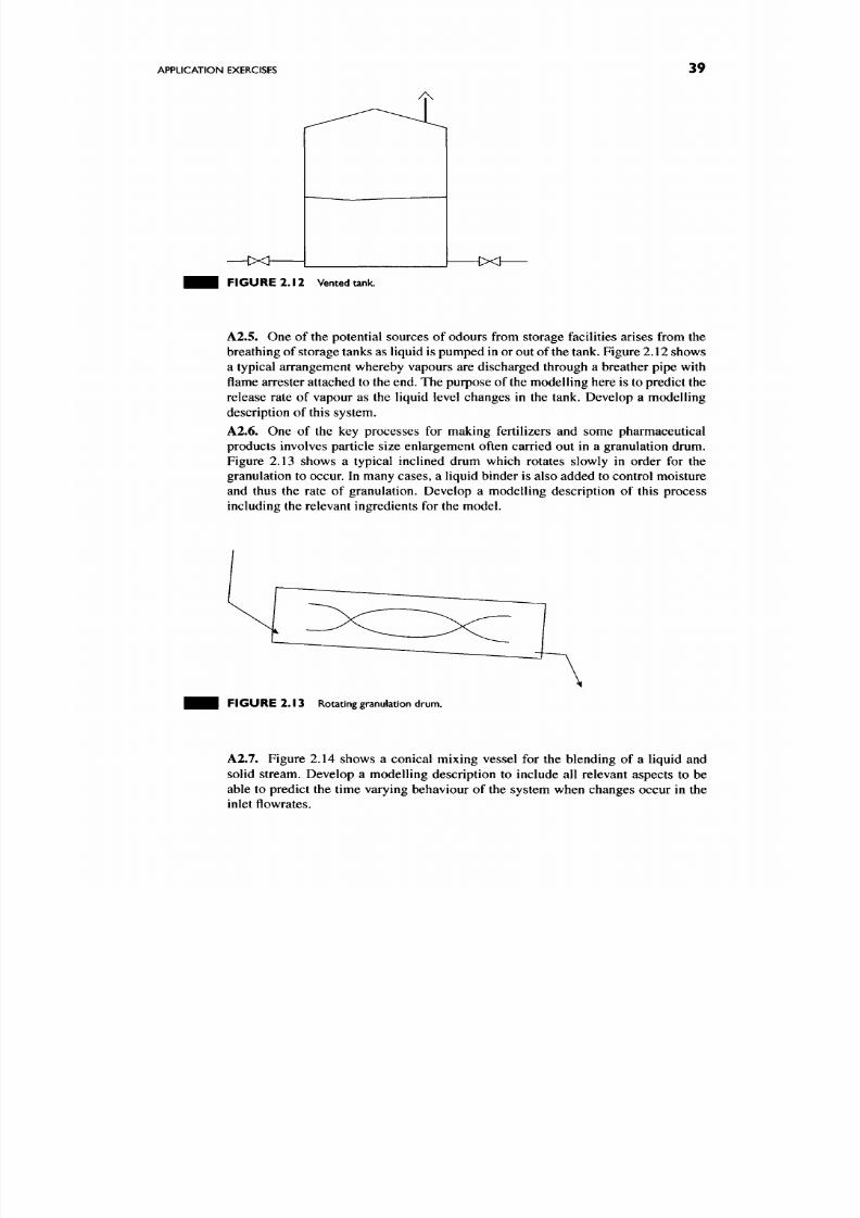
8/17/2019 Process Modelling and Model Analysis-Hangos-Cameron
http://slidepdf.com/reader/full/process-modelling-and-model-analysis-hangos-cameron 56/560
APPLICATION EXERCISES
39
— C X h
^x^
F I G U R E 2 . 1 2 Vented tank.
A2.5. One of the potential sources of odours from storage facilities arises from the
breathing of storage tanks as liquid is pum ped in or out of the tank. Figure 2.12 show s
a typical arrangement whereby vapours are discharged through a breather pipe with
flame arrester attached to the end. The purpose of the modelling here is to predict the
release rate of vapour as the liquid level changes in the tank. Develop a modelling
description of this system.
A2.6. One of the key processes for making fertilizers and som e pharm aceutical
products involves particle size enlargement often carried out in a granulation drum.
Figure 2.13 shows a typical inclined drum which rotates slowly in order for the
granulation to occur. In many cases, a liquid binder is also added to control moisture
and thus the rate of granulation. Develop a modelling description of this process
including the relevant ingredients for the model.
F I G U R E 2 . 1 3 Rotating granulation drum .
A2.7. Figure 2.14 show s a conical mixing vessel for the blending of a liquid and
solid stream. Develop a modelling description to include all relevant aspects to be
able to predict the time varying behaviour of the system when changes occur in the
inlet flowrates.

8/17/2019 Process Modelling and Model Analysis-Hangos-Cameron
http://slidepdf.com/reader/full/process-modelling-and-model-analysis-hangos-cameron 57/560
40
CHAPTER 2 A SYSTEMATIC APPROACH TO MO DEL BUILDING
F I G U R E 2.1 4 Conical blending tank.
A2.8.
Heat transfer is a key unit operation in the process industries. Figu re 2.15
shows a double-pipe heat exchanger for heat exchange between two liquid streams.
Consider the modelling of such a system for design and optimization purposes. How
would the model description change if stream temperatures change? Develop the
model description.
F I G U R E 2 .15 Double-pipe heat exchanger.
A2.9. Transport and storage of hazardous liquids is comm onplace in many areas
of modern society. Petroleum products and liquid chemicals such as solvents and
pesticides can pose significant h azards if released into the environment through loss of
containmen t from tanks. Consider the modelling of a pool of released solvent from the
rupture of a storage tank in the open air. The pool is subsequently contained in a bunded
enclosure around the tank. What are the key modelling ingredients which describe
the model? Develop a model description. What other issues must be addressed if the
spill is not bund ed?
8/17/2019 Process Modelling and Model Analysis-Hangos-Cameron
http://slidepdf.com/reader/full/process-modelling-and-model-analysis-hangos-cameron 58/560
CONSERVATION PRINCIPLES
In the previous chapter, we introduced a systematic approach to mathematical mod
elling. Following the establishment of the purpose of the modelling and the un derlying
assumptions about the system and its behaviour, the next step was the development
of the describing equations. One key aspect in this process is the application of con
servation principles
for conserved
extensive
quantities. Another important aspect is
the development of the constitutive relations which provide a set of relations which
are used to complete the model.
This chapter deals specifically with the underlying principles related to con
servation principles. This is based on the fundamental principle of physics that
mass, energy and momentum are neither destroyed nor created but simply change
their form. The relationship between extensive and intensive quantities is discussed
and the implications on their use in terms of model complexity and equation trans
formations are developed. T he focus of this chapter
is
on macroscopic thermodynamic
properties of process systems and how they are used for modelling purposes.
The application of conservation principles to typical gas-liquid-solid systems
normally leads to relationships involving total system mass, component masses, total
energy and system mom entum . In particulate systems , we can also consider q uantities
such as particle number balances for the generation of population balance equations.
This chapter de scribes the class of balance equations for total mass, component m asses
and energy. It covers the construction, general form and typical terms associated
with these balances. This chapter also discusses the implications of conservation
balances on the need for certain classes of constitutive equations for completing a
model description.
41

8/17/2019 Process Modelling and Model Analysis-Hangos-Cameron
http://slidepdf.com/reader/full/process-modelling-and-model-analysis-hangos-cameron 59/560
42 CHAPTER 3 CONSERVATION PRINCIPLES
It will become clear that in developing the conservation balances there are strong
connections to other general process engineering topics such as transport phenom
ena, reaction kinetics and reaction engineering. The details of these are given in
Chapter 4.
3.1.
THERMODYKAMIC PRINCIPLES OF PROCESS SYSTEMS
The underlying principles on which all process modelling takes place are based on
thermodynamic concepts [16,17]. Those thermodynamic concepts arise due to our
current understanding about the nature of matter, confirmed by ex periment and obser
vation. In particular, the fundamental laws of physics provide us with a framework
to describe the behaviour of systems through a consideration of the mass, energy
and momentum of the system in 3D space. We have to consider the fourth dimen
sion of time where we are also interested in the time varying behaviour of the
system.
3.1 .1 .
The Concept of a Space
For mod elling purposes, therm odynam ic pro perties are related to a defined region of
3D space which has an associated volume V and surface
T.
This region is usually
a
volume e ncapsulated by a closed surface which then defines the
region
of intere st for
the quantities of mass, energy and momentum.
It is sometimes termed the "balance
volume" or "control volume". Associated with this volume is a volume surface,
J^
which provides a connection to the surroundings or to other defined volumes of the
process.
We can also classify the type of region by considering the character of its con
nections to its environment. We can identify three main regions of interest forming a
system, namely,
•
Open systems,
where mass and energy can flow through the space of inter
est. These are the most common form of balance volume in PSE. Typical of
these processes are continuous flow reactors, or liquid-gas phase separation
systems.
• Closed systems, where there is no transfer of mass across the system bound
aries but energy may transfer. We can readily identify many engineering
systems w here this is the situation. Typical of this system w ould be the batch
reactor where there is no continuous addition of material during processing
but temperature of the batch is controlled. Energy transfers to or from the
contents.
• Isolated systems, w here there is no transfer of energy or mass ac ross the bound
aries.
Here the space under consideration is thermodynam ically isolated from
its surroundings. These are not common systems in the process industries.
Notice, however, that the volume V may change in time: think of a rising gas
bubble in a liquid being the region of interest.

8/17/2019 Process Modelling and Model Analysis-Hangos-Cameron
http://slidepdf.com/reader/full/process-modelling-and-model-analysis-hangos-cameron 60/560
THERMODYNAMIC PRINCIPLES OF
PROCESS SYSTEMS
43
F I G U R E 3 . 1 Fermentation tank and regions of interest (by permission of Stuart Range Estates).
Defining Regions of Interest
There are a number of ways in which we can define the regions of interest for our
process system. These include:
• The physical equipment volum es, which define distinct regions in space which
contain matter or energy. For example, the volume of a reactor in the case of
mass or in the case of energy, the walls of the vessel.
• The separate phases or states of aggregation in which m atter is identified. This
includes gaseous, liquid and solid states of aggregation.
In addition to defining the region of interest, it will be necessary to have an
associated local co-ordinate system with a defined origin, which allows us to locate
a particular point in space and thereby the value of a state.
Note that in defining the spaces of interest we have defined a process system
from the system theoretical viewpoint.
EXAMPLE 3.1.1 (Wine fermentation). In the case of grape juic e fermentation,
this is normally performed in stainless steel tanks similar to those shown in Fig. 3.1.
Within the fermenter, we can identify three distinct phases of interest which may be
used to develop a model based on conservation of mass and energy. These phases
are vapour, juice and lees (solids).
Figure 3.2 shows that in some cases we can have a mix of lumped or distributed
regions within the system of interest. We can also have levels of detail as seen in case s
(a) and (b).
Another example of a somewhat more "flexible" region of interest is a bubble in
a bulk liquid. Here, both the bub ble volume and the surface associated to it may vary
in time as the pressure and temperature in the bulk liquid around the bubble changes.

8/17/2019 Process Modelling and Model Analysis-Hangos-Cameron
http://slidepdf.com/reader/full/process-modelling-and-model-analysis-hangos-cameron 61/560
44
CHAPTER
3
CONSERVATION PRINCIPLES
feed
vapour
vapour
Lumped region
^ for vessel
Lumped region
for vapour
Lumped region
for liquid
Distributed region
for steam-
condensate
liquid liquid
Case (a) Case (b)
F I G U R E 3 . 2 Possible balance volumes fo r a process evaporator.
Co-ordinate Systems in Space
A point in space can be located by a vector which o riginates from the origin of the co
ordinate system and terminates at the point. These co-ordinate system s can be defined
in various ways. The most common systems in process engineering are given by:
• Cartesian or rectangular co -ordinates, wh ere a point in space is given by the
position along three co-ordinates: (jc,
y ,
z).
• Cylindrical co-ordinates, w here a point is identified by a radial dimension, an
angle of rotation and an axial distance: (r,
d, z),
• Spherical co-ordinates, where the point in space is given by a radial dimension,
an angle of rotation and an angle of elevation: (r,
d,
0) .
Figure 3.3 shows these basic co-ordinate systems and the definitions of the
governing measures to locate a point in space.
The choice of co-ordinate system is largely dictated by the underlying geometry
of the system being studied. For exam ple, the volume represented by a tubular reactor
can be easily considered in cylindrical co-ordinates, whereas the consideration of a
slab of material is likely to be represented in Cartesian co-ordinates. Also, certain
Rectangular Cylindrical
F I G U R E 3 . 3 Principal co-ord inate systems.
P{r,0,(l))
Spherical

8/17/2019 Process Modelling and Model Analysis-Hangos-Cameron
http://slidepdf.com/reader/full/process-modelling-and-model-analysis-hangos-cameron 62/560
THERMODYNAMIC PRINCIPLES OF PROCESS SYSTEMS
45
properties of the system which are functions of several spatial coordinates in one
system may only be a function of one co-ordinate in another system.
The two curvilinear co-ordinate systems of cylindrical and spherical geometry
can be related to the popular rectangular co-ordinates given by
x, y
and
z
through the
following relations:
Cylindrical co-ordinates:
X
= r cos(^), y = r sin(^), z = z,
or
yJx^-\-y^, ^ = a r c t a n ( - j , z — z.
Spherical co-ordinates:
X = r sin(0) cos(0) , y = r sin{6) s in(0) , z = r cos(^),
or
= V-^^ + J^ + z^, 0 = arctan ( — — j , 0 = arctan (-^ .
(3.1)
(3.2)
(3 .3)
(3 .4)
EXAMPLE 3.1.2 (Fixed bed reactor geometry). In Fig. 3.4, we see an industrial
fixed bed catalytic reactor for the hydrogenation of an unsaturated h ydrocarbon feed.
Reactants
flow
upw ards through beds of nickel based catalysts. Th e reaction takes
place throughou t the length of the bed and the obvious co-ord inate system for app lica
tion of mass and energy balances is cylindrical. It could be assumed that no variation
of concentration and temperature occurs in the angular direction 0. Variations often
occur in the radial direction, r.
F I G U R E 3 .4 Fixed bed catalytic rea cto r (by perm ission of Suncor Energy).
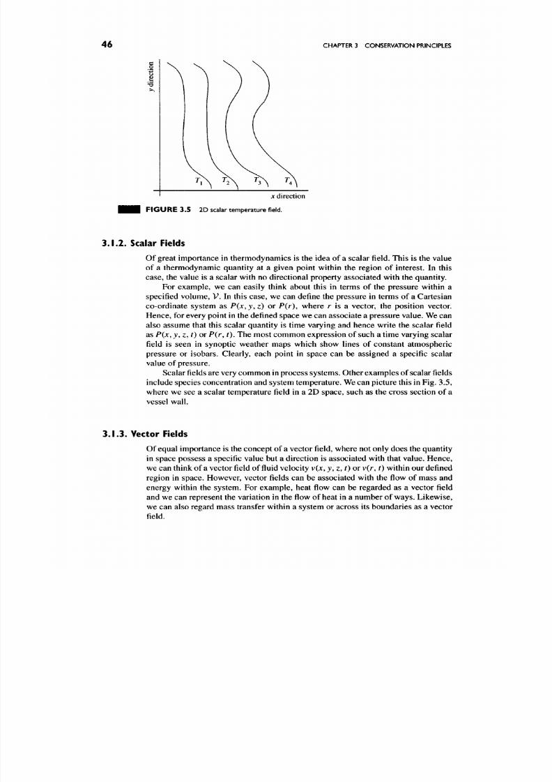
8/17/2019 Process Modelling and Model Analysis-Hangos-Cameron
http://slidepdf.com/reader/full/process-modelling-and-model-analysis-hangos-cameron 63/560
46
CHAPTER 3 CONSERVATION PRINCIPLES
X
direction
F I G U R E 3 . 5 2D scalar temperature field.
3.1.2. Scalar Fields
Of great im portance in therm odynam ics is the idea of a scalar field. This is the value
of a thermodynamic quantity at a given point within the region of interest. In this
case, the value is a scalar w ith no d irectional property associated w ith the quantity.
For example, we can easily think about this in terms of the pressure within a
specified volume, V. In this case, we can define the pressure in terms of a Cartesian
co-ordinate system as P(x, j , z) or P(r), where r is a vector, the position vector.
Hen ce, for every point in the defined space w e can associate a pressure value. We can
also assume that this scalar quantity is time varying and hence write the scalar field
as
P{x, y, z, t)
or P( r ,
t) .
The most common expression of such a time varying scalar
field is seen in synoptic weather maps which show lines of constant atmospheric
pressure or isobars. Clearly, each point in space can be assigned a specific scalar
value of pressure.
Scalar fields are very comm on in process system s. Other examples of scalar fields
include species concentration and system temp erature.
We
can picture this in Fig. 3.5,
where we see a scalar temperature field in a 2D space, such as the cross section of a
vessel wall.
3.1.3. Vector Fields
Of equal imp ortance is the concept of a vector field, where not only does the quan tity
in space possess a specific value but a direction is associated w ith that value. Hen ce,
we can think of a vector field of fluid veloc ity v(jc,
y, z, t)
or v(r,
t)
within our defined
region in space. However, vector fields can be associated with the flow of mass and
energy within the system. For example, heat flow can be regarded as a vector field
and we can rep resent the variation in the flow of heat in a number of ways. L ikewise,
we can also regard m ass transfer within a system or across its boundaries as a vector
field.
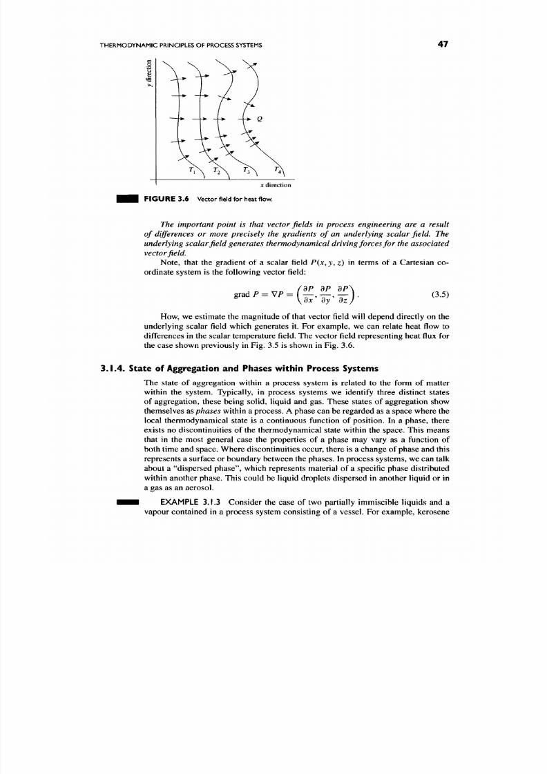
8/17/2019 Process Modelling and Model Analysis-Hangos-Cameron
http://slidepdf.com/reader/full/process-modelling-and-model-analysis-hangos-cameron 64/560
THERMODYNAMIC PRINCIPLES OF
PROCESS SYSTEMS
47
jc
direction
F I G U R E 3 . 6 Vector field for heat flow.
The important point is that vector fields in process engineering are a result
of differences or more precisely the gradients of an underlying scalar
field.
The
underlying scalar field generates thermodynam ical driving forces for the associated
vector
field.
Note, that the gradient of a scalar field P{x, y, z) in terms of a Cartesian co
ordinate system is the following vector field:
gradP = VP=(-,-,-j
(3.5)
How, we estimate the magnitude of that vector field will depend directly on the
underlying scalar field which generates it. For example, we can relate heat flow to
differences in the scalar temperature field. The vector field representing heat flux for
the case shown previously in Fig. 3.5 is shown in Fig. 3.6.
3.1.4. State of Aggregation and Phases within Process Systems
The state of aggregation within a process system is related to the form of matter
within the system. Typically, in process systems we identify three distinct states
of aggregation, these being solid, liquid and gas. These states of aggregation show
themselves as phases within a process. A phase can be regarded as a space where the
local thermodynamical state is a continuous function of position. In a phase, there
exists no discontinuities of the thermodynamical state within the space. This means
that in the most general case the properties of a phase may vary as a function of
both time and space. Where discontinuities occur, there is a change of phase and this
represents a surface or boundary between the phases. In process systems, we can talk
about a "dispersed phase", which represents material of a specific phase distributed
within another phase. This could be liquid droplets dispersed in another liquid or in
a gas as an aerosol.
• • • EXAMPLE 3.1.3 Consider the case of two partially immiscible liquids and a
vapour contained in a process system consisting of a vessel. For example, kerosene

8/17/2019 Process Modelling and Model Analysis-Hangos-Cameron
http://slidepdf.com/reader/full/process-modelling-and-model-analysis-hangos-cameron 65/560
48
CHAPTER 3 CONSERVATION PRINCIPLES
and water. Here, we could consider that there are three distinct phases within the
space of interest for the case of modelling the system dynamics. We have two liquid
phases (of different density) and a vapour phase . These phases can transfer bo th mass
•
• •
and energy between them depending on the thermody namic driving forces.
In some instances, we can further refine our definition of a phase by imposing
an equilibrium condition on the system. In this case, the phases consist of uniform
states in both time and space.
3.1.5. Extensive and Intensive Thermodynamic Properties
in
Process Systems
One of the basic distinctions in process modelling is between extensive (5 /) and
intensive (J/) thermodynamic properties. Extensive properties of a system are those
properties which depend on the extent of the system.
As such, the value of €( for the
who le of the region of interest is the sum of the values for all the parts in the system.
Such extensive properties include total mass and energy within the volume V, since
the mass or energy values for all the parts of the system must be added to get the
whole.
Extensive properties are strictly additive,
such that by composing a new system
S
by adding two systems
S\
and 52, the extensive properties of <S are the sum of the
extensive properties of S\ and S2 . Hence for property / we can write that
£ f
=sf' -\-£f\ 3.6)
There
is
also
a
canonical set of extensive quantities which
is
necessary and
sufficient to characterize a process system from a thermodynam ic view point. The set
can include total mass, volume, component masses, energy or enthalpy. The number
of extensive quantities needed to define the thermodynamical state of a system and
to determine all other macroscopic quantities depend on the individual system. The
canonical set of extensive quan tities can be viewed as thermo dynam ical state variables
to the process system.
In contrast to extensive properties, intensive properties do not depend on the
extent of the system.
In this case, the value changes from point to point in the system.
Typical intensive properties include temperature, pressure, densities and composi
tions.
Intensive properties are quantities which are typically m easured w ithin a process
system through the use of process sensors. As such they play an important role in
process modelling.
Also,
intensive properties will equilibrate if
we
add two systems
Si and «S2. In
this case, if we consider an intensive quantity Xf for the system S and we have, for
systems 5i and52,
if' < if'' (3.7)
then we can state that
if' <lf <lf\ (3.8)
In the case of a single component, single-phase system, an extensive property
can be expressed in terms of the system mass (M) and two intensive properties as:
€i=Mf(Ii,Ij).
(3.9)
8/17/2019 Process Modelling and Model Analysis-Hangos-Cameron
http://slidepdf.com/reader/full/process-modelling-and-model-analysis-hangos-cameron 66/560

8/17/2019 Process Modelling and Model Analysis-Hangos-Cameron
http://slidepdf.com/reader/full/process-modelling-and-model-analysis-hangos-cameron 67/560
50 CHAPTER 3 CONSERVATION PRINCIPLES
As well as being the typical measured quantities, intensive properties are those
used to express the degree of material and energy transfer between balance volumes
or diffusive flow within balance volum es.
Material and energy flows or transfer rates are typically vector fields with an
underlying scalar field of an intensive variable generating a thermo dynam ical driving
force for them. The underlying intensive variable of the flow or transfer rate of an
extensive property is called the potential related to it.
For example, heat flow is related to changes in the field value of temperature,
whereas mass transfer is related to variations in chemical potential or concen trations.
These are intensive properties. Therefore, we can say that
tem perature is the poten
tial to internal energy or enthalpy and che mical potential is the potential related to
component mass.
3.1.6. Phases and Independent Intensive Quantities
It has been mentioned that only two intensive quantities are needed to enable all
other intensive quantities to be determined in a single phase, pure compon ent system .
These specifications are known as the thermodynamic degrees of freedom of the
system. We can generalize this concept to any number of phases using the phase rule
first formulated by Gibbs. For non-reacting systems where there are n components
and 7t phases, the degrees of freedom (DOF)
F
(or independent intensive quantities)
to be specified are
F = n + 2-7t . (3.14)
In the case where there are v independent reactions taking place, we have
F = n + 2 - 7 r - v . (3.15)
In some cases, this can be reduced further when we impose other constraints on
the system.
• • • EXAMPLE 3.1.6 Consider the case of a two component system, where there
are two liquid phases and a vapour phase. What number of independent intensive
variables can be specified for this system?
Butanol-water is such a system. Here,
F = n-{-2-n
with
n = 2 JT = 3,
so that
F = 2 - h 2 - 3 = 1.
• • • In this case, we can only specify one intensive quantity.
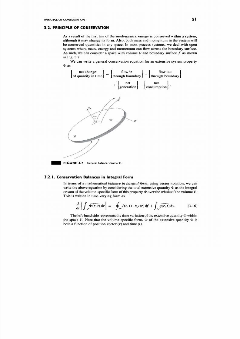
8/17/2019 Process Modelling and Model Analysis-Hangos-Cameron
http://slidepdf.com/reader/full/process-modelling-and-model-analysis-hangos-cameron 68/560
PRINCIPLE OF CONSERVATION
3.2. PRINCIPLE OF CONSERVATION
51
As a result of the first law of thermodynamics, energy is conserved within a system,
although it may chang e its form. Also, both mass and m omentum in the system will
be conserved quantities in any space. In most process systems, we deal with open
systems where mass , energy and momentum can flow across the boundary surface.
As such, we can consider a space with volume V and boundary surface
T
as shown
in Fig. 3.7
We can write a general conservation equation for an extensive system property
<I> as
net change
of quantity in time
{
f low in I I flow ou t 1
through boundary J [ through boundary J
-f
net
1-1
net
1
I generation
J
[ consumption
J
F I G U R E 3 . 7 General balance volume V.
3.2 .1 .
Conservation Balances in Integral Form
In terms of a mathematical balance in integral form, using vector notation, we can
write the above equation by co nsidering the total extensive quantity <1> as the integral
or sum of the volume-specific form of this property <> over the whole of the volume V .
This is written in time varying form as
Odv =
J ( r , O n j r ( r ) d / + / q(rj)dv.
J V
(3.16)
The left-hand side represents the time variation of the extensive quantity ^ within
the spac e V. No te that the volume-specific form, 4> of the extensive quantity 4> is
both a function of position vector (r) and time
(t).
8/17/2019 Process Modelling and Model Analysis-Hangos-Cameron
http://slidepdf.com/reader/full/process-modelling-and-model-analysis-hangos-cameron 69/560
52 CHAPTER 3 CONSERVATION PRINCIPLES
The first term on the right-hand side accoun ts for the flow of the extensive quantity
through the total closed boundary of the surface
T.
It thus accou nts for inflow and
outflow from the volume under consideration. It consists of the value of the flow
y (r, r ), w hich is a vector field varying from point to point on the surface
T ,
integrated
over the whole closed surface. H ere, the
flow
s regarded
as
passing through a unit area
of the surface with an outward pointing unit (normal) vector n jr perpen dicular to that
surface. The normal vector is clearly a function of spatial position as w e integrate over
the complete surface. This term accounts for all possible modes of transfer through
the closed surface. These could be c onvective or diffusive in nature.
The last term represents the net consum ption or generation of the extensive quan
tity within the specified vo lume. This is typically related to energy or species sources or
sinks associated with reactions in the system and is represented by the volume-specific
source
q{r, i).
3.2.2.
Conservation Balances in Differential Form
In the limit, as V becom es infinitesimally small, we can w rite the above equation
in
differential form after applying the G auss divergence theorem to the surface integral
to convert it to a volume integral. This is the usual form of the balance equation we
see in most process modelling situations. We obtain
• ^ = - V . y + , , (3.17)
where the divergence o f/ is given by
^Jx dJx dJ?
V . y = d iv (y ) = - ^ + - ^ + - r^ , (3 .18)
dx dy dz
where
Jx, Jy
and
J^
are the three components of the flow
J
in the direction of the
principal co -ordinates. N ote that the divergence of a vector field is a scalar field. This
form of the balance equation is scalar in all terms.
Flow or Transport Terms
We have already con sidered in the general conservation equation that flows can enter
and leave the volume V . These flows can be of two general forms:
• convective flows,
JQ,
• diffusive or mo lecular flows, D -
Hence in the case of mass, the total flow/ can be written as the sum of convective
and molecular flows:
y = y c + «/D, (3.19)
where w e can define the individual flow comp onents as
yc = cD (r,r )v( r ,0 , (3.20)
JD = -Dgrad (p(r, t) = -D W(p(r, t) . (3.21)

8/17/2019 Process Modelling and Model Analysis-Hangos-Cameron
http://slidepdf.com/reader/full/process-modelling-and-model-analysis-hangos-cameron 70/560
PRINCIPLE OF CONSERVATION
53
Note that in the definition of the convective flow, the vector v(r, t) is used to
describe the convective flow pattern into or out of the system volume V. This vector
wiU typically be the velocity components of the flow in the appropriate co-ordinate
system. The velocity components of the vector v(r, t) can in principle be computed
from the general transport equation for the system via a momentum conservation
balance . In practice, however, simp le flow patterns, such as plug flow or laminar flow
are most often used which are stated as modelling assumptions.
Hence, for the overall mass balance in volume V, we can write the differential
conservation balance as
^ = - V . (pv), (3.22)
01
where
p
is the volume-specific mass and v is the velocity vector.
Note also, that the diffusive flow
J D
is an approxim ate relation involving a diffu
sion coefficient
D
and the gradient of the potential (p(r,
t)
which corresponds to the
equivalent extensive property O. For example, when considering the diffusive molar
flow of a species we can consider the driving force or potential to be the chemical
potential of the species in the system. This is often reduced to the intensive quantity of
molar co ncentration of the particular spec ies. In the above relation for diffusive flow
the cross terms (interaction term s) have been neglected. This can be vitally impo rtant
in multi-component systems w here the Stefan-Max well relations should be applied.
Hence, for the component / mass balance with no reaction we have
^ = - V - ( p / v + 7 / ) , (3 .2 3)
ot
where p / is the com ponent / volume-specific mass andy, is the diffusional flux vector.
Source Terms
The final term in the general conservation equation given by
q{r, t)
is related to
sources or sinks of mass, energy or momentum in the system. This term can arise in
various ways including:
• Chem ical reaction for com ponent mass conservation, wh ere species appear or
are consumed due to reactions within the space of interest. This is an
internal
source term.
• Other
internal
source terms arise from energy dissipation or conversion plus
compressibility or density changes.
• External energy sources include gravitational, electrical and magnetic fields
as well as pressure fields.
It is clearly im portant to identify the key m echanism s in the space under cons id
eration in order to capture the principal contributions to the source terms represented
by q{r, t). Note that the source term represented by q{r, t) almost always depends on
the potential ^(r,
t)
which corresponds to the equivalent extensive properties char
acterizing our process system. Think of the dependence of the reaction rate on the
temperature and compo sitions.
For the component / mass balance with chemical reaction we have
M = _v.(p,v+;• , . )+ r,-, (3.24)
8/17/2019 Process Modelling and Model Analysis-Hangos-Cameron
http://slidepdf.com/reader/full/process-modelling-and-model-analysis-hangos-cameron 71/560
54
CHAPTER 3 CONSERVATION PRINCIPLES
where pi is the component / volume-specific mass, ji is the diffusional flux vector
and r/ is the rate of generation or disappearance of species /, being equivalent to the
source term q(r, t).
It is possible to develop further conservation equations for total energy and
mom entum. In the case of conservation b alances for vector quantities like mo mentum
the balance equations can be quite complex . The interested reader is referred to the
seminal w ork of Bird etal. [13] to obtain com plete expressions in various co-ordinate
systems.
Potential Variable Relations
As has been emphasized before, the potential (p which co rresponds to the equivalent
extensive property 4> is necessarily p resent in the con servation balance equ ations if
we have either transfer or source terms or both. Therefore, we need to add consti
tutive equations relating potentials to volume-specific extensive variables to make
our process model complete.
These constitutive equations are called
potential vari
able relations and are usually in the form of algebraic equations between intensive
variables, like those shown in (3.12).
Particulate Systems
It is convenient in the context of conservation principles to also mention that dis
crete entities such as particle numbers are subject to conservation principles. This
leads to the concept of "population balances". The concepts of conserved quanti
ties in particulate systems has widespread application in minerals processing, food,
pharmaceuticals and the chemical industries.
In the case of population based ba lances, the properties of the materials are char
acterized by population density functions (distribution functions) instead of a scalar
quantity. To use this approach, the distribution function must contain information
about the independent p roperties of the system. In this case, the particle co-ordinates
are divided into external and internal co-ordinates where the external co-ordinates
refer to the spatial distribution of the particles and the internal co-ordinates refer to the
properties attached to the particles such as size, shape, age or chemical com position.
The distribution function could be expressed as
n ( r , x , j , z , C i , f 2 , . . . , ? m ) , ( 3 .2 5 )
where
m
is the number of internal co-ordinates ^ i, 2 • • •» ?m being used. In a manner
similar to that for the integral form of the conservation balance we can w rite
j l j n{t ,x)dv\=j {B(t .x)-D(t .x))dv, (3.26)
where
B
and
D
are birth and death terms for the system and
x = [ r , x , j ,
z,
?b?2» ••-.?/«]•
Man ipulation of the general balance equation leads to the microscopic population
balance:
^ = - V . ( v n ) + ^ - D , (3.27)
ot
8/17/2019 Process Modelling and Model Analysis-Hangos-Cameron
http://slidepdf.com/reader/full/process-modelling-and-model-analysis-hangos-cameron 72/560
PRINCIPLE OF CONSERVATION
55
where
n
is the number density function, being the number of particles per unit volume
at time t. Other terms covering nucleation and breakage can also be included. Typ
ically, the birth and death terms B, D are described by integral terms which include
special kernel functions as seen in the following example.
• • • EXAMPLE 3.2.1 (Granulation system modelling). In modelling the behaviour
of granulation drums for the production of fertilizer, Adetayo
et al.
[18] used a
population balance approach to predict the particle size distribution as a function
of position and time. This involved the general population balance equation given
by (3.27).
The general balance for the batch drum was given as
— ^ = 5 ( v , 0 - / ) ( v , 0 , (3.28)
where v is the particle volume, and the birth and death terms are given by
1 r~
JB(V, 0 = ——— / piv -
M,
u)n{u, t)n(v - M, t)
dw,
(3.29)
2N{t)
Jo
1 r
^ ( ^ '
0 = -T77T / P(^^ ")^ (" ' ^)^(^ ' 0
dM.
(3.30)
J^U)
Jo
The coalescence kernel p can take various forms which reflect the understanding of
the growth process. These include a continuous form suggested by Kapur [19]:
P(u. V) = Po
Uu
+ vr
(3.31)
or a multi-stage, switched kernel given by Adetayo [20] as
(/(mo isture) r < ^sl (3 3^ )
1 / (w, v) t>tsi
switching at time fsi •
The General Operator Form of the Conservation Equation in Differential Form
We can consider the general differential conservation exp ression given by Eq. (3.17)
by expanding the terms as follows:
^ + V . ( y c + / D ) = ^ . (3 .3 3)
This can be further expanded by considering the form of the individual flow
components in Eqs. (3.20) and (3.21) to obtain
^ + V .
($0^)
v(r , 0 ) - V .
(D Vcpir, t)) = q.
(3.34)
The above equation can be rearranged using that
D
= constant to get
^ = D V . (V ^(r , 0 ) - V . (<I)(r, t ) v(r, r)) + q. (3.35)

8/17/2019 Process Modelling and Model Analysis-Hangos-Cameron
http://slidepdf.com/reader/full/process-modelling-and-model-analysis-hangos-cameron 73/560

8/17/2019 Process Modelling and Model Analysis-Hangos-Cameron
http://slidepdf.com/reader/full/process-modelling-and-model-analysis-hangos-cameron 74/560
PRINCIPLE OF CONSERVATION
57
The component mass and energy conservation equations written for the volume-
specific component mass (i.e. for the molar concentration) c and for the volume-
specific internal energy and
U
are given by
where AHR is the reaction enthalpy. Note that the convective term is missing because
there is no convection within a pellet.
Observ e the form of the diffusion term expressed in spherical co-ordinate system
being the first term on the left-hand side of the equation.
Moreover, the potential relation for the temperature can be written as
U = U(T,c), (3.41)
Clearly, the two conservation eq uations are closely cou pled through the reaction term
which ap pears in both equations . Both equations are parabolic type partial differential
equations in nature.
Observ e that we do not have any transfer term and the volume-specific source is
• • • identical to the reaction rate expression in this case.
3.2.4.
Model Classes in Mathematical Terms
We can survey the types of mathematical models that arise from the application of
conservation princ iples. Here, we can subdivide the problem into dynamic and steady-
state models where either type can be distributed or lumped in nature. We can derive
special forms of the general conservation equation (3.37) by applying mathematical
transformations expressing our engineering assumptions of a system being dynamic
or steady state, lumped or distributed parameter. In this manner, we can generate the
various model equation forms which appear in Table 1.3.
• • • EXAMPLE 3.2.3 (Distributed parameter static model form). Consider the gen
eral conservation equation (3.37) and assume, that there is no time variation in the
system, i.e. the system is static. Then
ao ^
w
=
-
We now get the following special form:
a2^^
o2^^ i\2
a > a > d^(p\ d<t>vx d^vy d^v
which is indeed an elliptic partial differential equation (E PD E) (cf. row 4 in Table 1.3).
M ore about the different process m odels in partial differential equation form will
follow in Section 7.3.

8/17/2019 Process Modelling and Model Analysis-Hangos-Cameron
http://slidepdf.com/reader/full/process-modelling-and-model-analysis-hangos-cameron 75/560
58
CHAPTERS CONSERVATION PRINCIPLES
The Induced Algebraic Equations
We have already mentioned before in Section 3.2.2 that the conservation calls
for algebraic equations to make the formulated balance equation complete. These
equations appear in the various classes of constitutive equations, such as
• potential variable relations— relating conserved extensive quantities and their
associated potentials,
• source terms— relating the volume-specific source terms to the potential scalar
fields of the system.
Mo re about the constitutive equ ations w ill follow in Chapter 4.
3.3. BALANCE VOLUMES
IN
PROCESS SYSTEM APPLICATIONS
The role of balance volumes for mass, energy and momentum is crucial in process
mod elling. A balance volume is a basic element in process m odelling as it determines
the
region in which the conserved quantity
is
contained. H ow are these regions chosen?
Clearly, there are many possibilities. Figure 3.8 shows a simple evaporator vessel
where liquid is being heated to produce a vapour. As can be seen, there are several
options in the choice of the mass balance boundaries, given by the symbol Ylf -
Balance Volumes and the Modelling Goal
Case (a) looks at developing the balances around the complete vessel, whereas case (b)
considers each phase as a separate balance volume. In the second case, there will be
mass and energy flows between the two balance volumes.
We co uld also consider other possibilities dependent on the degree of complexity
demanded and on the characterizing variables called by the modelling goal. These
could include mass balance volumes around bubbles within the liquid phase if mass
transfer were an issue in multi-component systems.
In general, parts of a process system which are typical candidates for balance
volume definition include those regions which:
• contain only one phase or pseudo -phase,
• can be assumed to be perfectly m ixed, or
• can be assumed to have a uniform (homo geneous) flow pattern.
We use the term "pseudo-phase" for a region which we have coalesced for
purposes of model simplification and the application of conservation balances. A
pseudo-phase could constitute several distinct phases regarded as a single entity for
modelling purposes.
Besides the thermodyn amical and
flow
characteristics of the process system to be
modelled the modelling g oal can and will direct us to find the relevant set of balance
volumes for the given modelling problem. The most common modelling goals were
described and characterized in Section 2.1 in general terms. In a concrete modelling
case the m odelling goal, when properly stated, implies
• The requested precision (accuracy) of the mo del output thus determining the
level of detail of the model. More about process models of the same system

8/17/2019 Process Modelling and Model Analysis-Hangos-Cameron
http://slidepdf.com/reader/full/process-modelling-and-model-analysis-hangos-cameron 76/560
8/17/2019 Process Modelling and Model Analysis-Hangos-Cameron
http://slidepdf.com/reader/full/process-modelling-and-model-analysis-hangos-cameron 77/560
60
CHAPTERS CONSERVATION PRINCIPLES
mass balance volumes. There are significant implications in this type of definition.
Let us formalize this concept.
A process system can be modelled based on a set of balance volumes, E. The
full set consists of p subsets associated with the conserved qua ntities, such as overall
and component m asses, momentum and energy. Note that component m ass balances
are not independent of the overall mass balance, since the full set of component
balances will sum to the total balance. This leads to problems of overspecification
and subsequent numerical difficulties. All the mass balances, component and total
balances should be setup over the same mass balance region. Therefore, we only
consider a single balance volume set for all the mass balances.
We can consider three major conserved quantities (mass (^), energy (^), and
momentum (^^), i .e .
p =
3). The full balance volume set E for a given modelling
situation is then given by
E = E ^ U S^ U E ^ ^ , (3 .43)
where the individual boundary sets are
E ^ = [ E f , . . . , E ^ j E^ = JEf,...,E^ ) E^^ = [ E r , . . . , E r ) .
(3.44)
As mentioned previously, it is important to note that energy balance volumes may
include several full mass balance volumes, but none of the mass balance volumes
contain more than one corresponding energy balance volume. Therefore,
N < M
indicates that the mass balance volumes are primary balance volumes. There may,
of course, be other independent energy balance volumes defined apart from those
associated with mass holdups.
Furthermore, it is also important that the relation above puts restrictions on the
corresponding energy balance volumes, if a new mass balance volume is formed by
coalescence
of several individual mass balance volumes. Coalescence in this context
is the result of merging or fusing together distinct balance volumes into a single
volume with homogeneous properties.
It is important to note that spatial and neighbouring relations can also be very
important when formulating distributed parameter process models. These relations
give relations between boundary conditions of the individual conservation equations
over the balance volum es. More abou t this problem can be found in Chapters 7 and 9.
• • • EXAMPLE 3.3.1 (Distillation column with trays). Figure 3.9 shows a typical
industrial distillation column for hydrocarbon separations. The normal balance vol
ume is shown as the plate p w ith various vapour and liquid flows arriving and leaving
an individual stage. By aggregating all stages 1,..., n in the column, a full model is
developed.
• • • In this case, the balance volume is a lumped region.
I H H EXAMPLE 3.3.2 (Shell and tube heat exchan ger). Figure 3.10 shows an indus
trial shell and tube h eat exchanger and a typical balance volume for fluid in the tubes.
This is a distributed parameter system with
z
representing the axial distance from
the tube entry. Both the tube liquid 7L and coolant TQ are functions of time and
• • • position.

8/17/2019 Process Modelling and Model Analysis-Hangos-Cameron
http://slidepdf.com/reader/full/process-modelling-and-model-analysis-hangos-cameron 78/560
SUMMARY
61
'^^j
?y<1
p
V
P-1
T
p
A
•
V+1
F I G U R E 3 .9 industr ial dist i l lat ion colum n (by permission of Caltex).
F I G U R E 3 .1 0 Industr ial shell and tube heat exchanger (by permission of Calte x).
3.4. SUMMARY
In this chapter, we have dealt with the basic underlying principles of conservation
applied to mass, energy and momentum. These principles form the basis for any
mod elling task. It was also shown that the quantities that are of interest can be classed
as extensive and intensive. It is the extensive properties that constitute the role of
conserved qu antities whereas the intensive properties provide the basis for com puting
driving forces for material and energy transfer in the system.
The importance of the various co-ordinate systems in either rectangular, cylin
drical or spherical geometry were introduced and their implications for modelling
discussed. The final model form will be dependent on the assumed geometry of the
system und er study. This is a matter of judge me nt for the m odeller but, generally, the
physical or chemical phenomena will dictate the approach to be taken.
Finally, the definition of balance volumes in process engineering applications
was considered, show ing that there are indeed m any ways of defining balanc es. Mo st,

8/17/2019 Process Modelling and Model Analysis-Hangos-Cameron
http://slidepdf.com/reader/full/process-modelling-and-model-analysis-hangos-cameron 79/560
62
CHAPTERS CONSERVATION PRINCIPLES
however, are dictated by the identification of system phases in which there is a condi
tion of homogeneity. The next chapter introduces the con cept of constitutive relations
and definitions which are an important class of relations to help complete the full
model description. Subsequent chapters then develop out the principles in particular
application areas.
3.5. REVIEW QUESTIONS
Q3.1.
Describe the difference between open, closed and isolated system s. Wh at are
process engineering examples of these systems? (Section 3.1)
Q3.2. What are the fundamental differences between scalar and vector fields. List
examp les of both types of fields? (Section 3.1)
Q3.3.
Describe the role of intensive and extensive variables within
a
process system.
What controls the independent specification of intensive variables for a particular
system? (Section 3.1)
Q3.4.
What role do balance volumes play in process mod elling? Discuss ways in
which they can be defined? (Section 3.3)
Q3.5.
Wh at role does the conservation principle play in mod elling. In what two
fundamental forms does the principle appear? Discuss the reasons that lead to these
forms.
(Section 3.2)
Q3.6. Wh at are the principal terms that can appear within the conservation balance
equation? W hat form do these terms take and how are they related to the physics and
chemistry of the application? (Section 3.2)
Q3.7. Describe the role which conservation balances play in the mathem atical
modelling of process systems. (Section 3.3)
Q3.8. What are the key issues in deciding the location of balance volumes for a
modelling application? (Section 3.3)
Q3.9.
Why is it that energy balance volume s are normally coincident with
mass balance volumes? Is there a natural hierarchy in defining balance volumes?
(Section 3.3)
Q3.10. What are the implications of defining energy balance volumes which
encompass several mass balance volumes? (Section 3.3)
3.6. APPLICATION EXERCISES
A3.1.
For the case of
the
open tank given in Exercise
A2.1
and illustrated in Fig. 2.8,
discuss and define the likely balance volumes that could be used for the modelling
problem. W hat are the principal characterizing variables given that we are interested
in modelling the liquid level dynamics?
A3.2. Consider the balance volume definitions for the case of the closed tank problem
dealt with in Exercise
A2.2.
How has this new process situation changed the potential
balance volume definitions and what if anything is the relationship between balance
volumes?
8/17/2019 Process Modelling and Model Analysis-Hangos-Cameron
http://slidepdf.com/reader/full/process-modelling-and-model-analysis-hangos-cameron 80/560

8/17/2019 Process Modelling and Model Analysis-Hangos-Cameron
http://slidepdf.com/reader/full/process-modelling-and-model-analysis-hangos-cameron 81/560
8/17/2019 Process Modelling and Model Analysis-Hangos-Cameron
http://slidepdf.com/reader/full/process-modelling-and-model-analysis-hangos-cameron 82/560
CONSTITUTIVE RELATIONS
Constitutive relations are usually algebraic equations of mixed origin. The u nderlying
basic thermod ynam ic, kinetic, control and design knowledg e is formulated and added
to the conservation balances as constitutive equations. This is because when we write
conservation balances for mass, energy and momentum, there will be terms in the
equations which will require definition or calculation. These requirements give rise
to a range of constitutive equations which are specific to the problem.
Constitutive equations describe five classes of relations in a model:
•
transfer rates:
mass transfer, heat/energy transfer;
• reaction rate exp ressions;
• property relations: thermodynamical constraints and relations, such as the
depen dence of thermodynam ical properties on the thermo dynam ical state vari
ables of temperature, pressure and composition. There are also equilibrium
relations and equations of state;
• balance volume relations: relationships between the defined mass and energy
balance regions;
• equipment and control constraints.
These constitutive equation classes are shown in Fig. 4.1.
4 . 1 . TRANSFER RATE EQUATIONS
In many applications of the conservation principles for mass, energy and momentum
there will be cases where m ass, energy or mom entum will be transferred into or out of
65
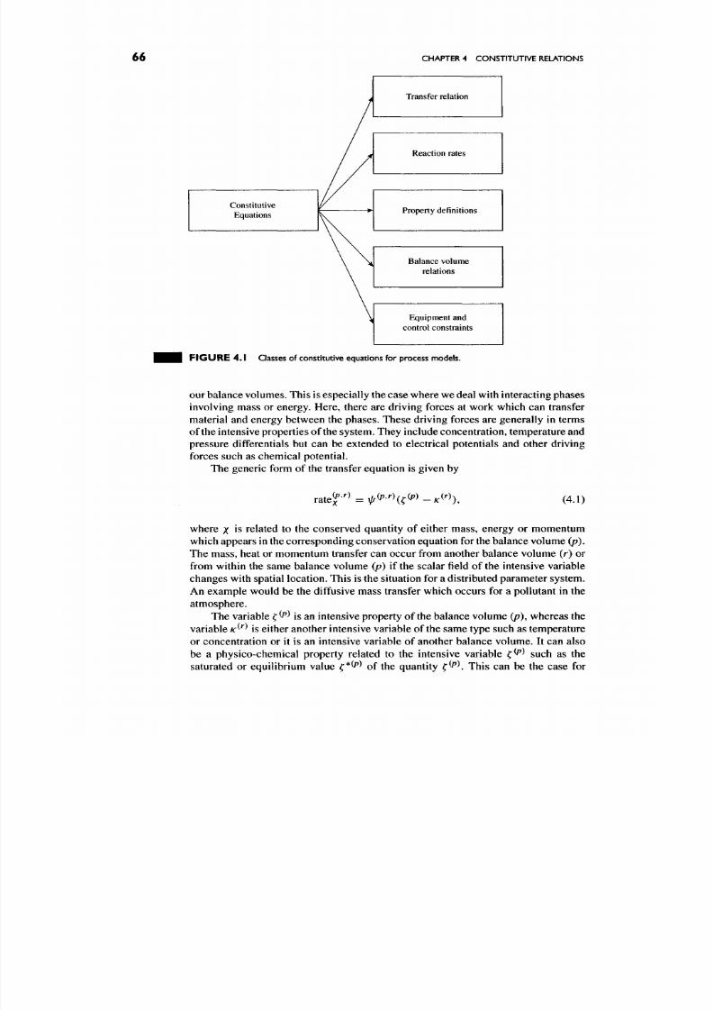
8/17/2019 Process Modelling and Model Analysis-Hangos-Cameron
http://slidepdf.com/reader/full/process-modelling-and-model-analysis-hangos-cameron 83/560
66
CHAPTER 4 CON STITUTIVE RELATIONS
Constitutive
Equations
Transfer relation
Reaction rates
Property definitions
Balance volume
relations
Equipment and
control constraints
F I G U R E 4 .1 Classes of con stitutiv e equations fo r process mod els.
our balance volum es. This is especially the case where we deal with interacting ph ases
involving mass or energy. Here, there are driving forces at work which can transfer
material and energy between the phases. These driving forces are generally in terms
of the intensive properties of the system. They include con centration, tem perature and
pressure differentials but can be extended to electrical potentials and other driving
forces such as chemical potential.
The generic form of the transfer equ ation is given by
ratef''^ =
V^(P^'')(^(P)
Ar)
),
(4.1)
where x is related to the conserved quantity of either mass, energy or momentum
which appears in the correspon ding co nservation equation for the balance volume (p).
The mass, heat or momentum transfer can occur from another balance volume (r) or
from within the same balance volume (p ) if the scalar field of the intensive variable
changes with spatial location. This is the situation for a distributed parameter system.
An exam ple would be the diffusive mass transfer which occurs for a pollutant in the
atmosphere.
The variable f ^^ is an intensive property of the balance volume (p), w hereas the
variable
K ^ ^ ^
is either another intensive variable of
the
same type such as temperature
or concentration or it is an intensive variable of another balance volume. It can also
be a physico-chemical property related to the intensive variable ^^^ such as the
saturated or equilibrium value ^*^^ of the quantity
^^ \
This can be the case for

8/17/2019 Process Modelling and Model Analysis-Hangos-Cameron
http://slidepdf.com/reader/full/process-modelling-and-model-analysis-hangos-cameron 84/560
TRANSFER
RATE
EQUATIONS
67
mass transfer represen ted by the two-film mod el, where the driving force involves the
bulk concentration and the concentration at the interface.
It is impo rtant to note that transfer can be in both direc tions. It can be to balan ce
volume
(p),
or from balance volume
(p )
to another balance volume (r). This can
be taken into account in the model. The driving force (f
^^
—
K ^ ^ ^ )
is the same for
both directions of transfer but the transfer coefficients, ^^''^ and xl/^^'^P may differ.
Moreover, both transfer coefficients can be functions of the thermodynamical state
variables in the two balance volumes, (p ) and (r).
We now consider two specific instances of these types of interphase transfer.
4 . 1 . 1 .
Mass Transfer
Mass transfer involves a driving force in terms of chemical potential or equivalent
intensive property such as concentration or partial pressu re. The fundamental c oncept
involves Pick 's Law which describes the
flux
of
a
component
(j )
in terms of
a
diffusion
coefficient D and a concentration gradient, dC/dz. It is given by
j = -D
.dC
d z '
(4 .2)
where typical units arery [kg • m~^ s~*],
D
[vcr s~M»
C
[kg • m~^], dz [m].
Typically, a two-film theory is proposed to describe the mass transfer process,
where an interface (/) between th e two phases is defined as w ell as bulk and interface
concentrations for both phases. The films have theoretical thicknesses, C/L and (IQ.
This situation is seen in Fig. 4.2.
iquid phase
1^ ^
: ^ L
; 1
1 gas phase
^
1 Co
do
*'
F I G U R E 4 . 2 Two-film schematic fo r mass transfer.

8/17/2019 Process Modelling and Model Analysis-Hangos-Cameron
http://slidepdf.com/reader/full/process-modelling-and-model-analysis-hangos-cameron 85/560
6 8 CHAPTER 4 CONSTITUTIVE RELATIONS
The mass flux 7 can be written for each side of the film and equated assuming no
accumu lation at the interface to give
( C L
-
C\
)
{Cr -
C G )
j =
DL'
^ . ^ ' = ^G ^ , (4.3)
or in terms of film mass transfer coefficients:
j = kL(CL - C[) = kciCi. -
CG) ,
(4.4)
where the mass transfer coefficients are defined as follows:
DL
kL=^-r.
(4.5)
^G = ^ . (4.6)
«G
Sometimes the total mass flux, J is defined based on the available transfer area
A
[m^], such that
J=jA.
(4.7)
or in terms of specific surface area
a
[m^/m^] such that
J=j'(aV) (4.8)
with
V
being the volume.
It is then possible to write Eq. (4 .4) as a total flux equa tion:
J = kLa(CL -
C[)V =
kcaiCi. -
C G )V .
(4.9)
The combined terms of ki^a and kQ a are often those quoted in the mass transfer
literature.
The problem w ith these equation forms is that the interface conc entrations cannot
be measured and the flux should be w ritten in terms of measurable or easily com puted
quantities. To help achieve this, w e can use the equ ilibrium relationship
CQ
=f(CO
to write the mass transfer in terms of an overall mass transfer coefficient,
KQ,
giving
for Eq. (4.4) the equivalent of:
j = kLiCL - C[) =
kGiC[.
- CG) = KG{C^ - CG) (4.10)
with
KG kG k^
Here, m is the slope of the equilibrium line and CQ is the gas phase concentra
tion in equilibrium with the bulk liquid phase concentration
CL.
Hence, most mass
transfer can be written in terms of a concentration driving force and an overall mass
transfer coefficient which is computed from correlations for the film mass transfer
coefficients. Correlations for particular applications are found in [21] or standard
mass transfer texts. Multi-component mass transfer is, in principle, more complex
and correct approaches make use of the Stefan-Maxwell equation. There are several
simplifications to the general approach w hich can make the mod elling m ore tractable
but at the expense of model accuracy. The reader is referred to the book by Taylor
and Krishna [22] for a full discussion on this topic.
8/17/2019 Process Modelling and Model Analysis-Hangos-Cameron
http://slidepdf.com/reader/full/process-modelling-and-model-analysis-hangos-cameron 86/560
TRANSFER RATE EQUATIONS 69
4.1.2. Heat Transfer
Heat transfer takes place through the three principal mechanisms: conduction, radi
ation and convection. Each mechanism can be represented by specific forms of
constitutive equations. Th e following g ives
a
brief outline of the principal heat transfer
mechanisms and their mathematical representation.
Conduction
The rate of heat transfer by conduc tion is governed by the fundamental expression of
Fourier given by
^CD = -kA (4.12)
which describes the energy transfer ^CD [J • s~^ or W] in terms of a thermal conduc
tivity,
k
[J/s
•
m
•
K ], a heat transfer area,
A
[m^] and a temperature gradient
dT/dx
[K/m]. This general heat transfer relation (4.12) can be integrated across the medium
of conduction to give
r
qCD(ix
= -kA [ 'dT (4.13)
Jo JTi
or
qcu^-(Ti-T2)
=
- (4.14)
X x/{kA)
The term
x/(kA)
in Eq. (4.14) is the thermal resistance to heat transfer and has
units of/iT/W.
The form of the driving force will vary depend ing on the situation. For c ondens ing
steam with no subcooling of condensate the driving force is simply the difference
between the steam temperature and the fluid temperature. For situations where the
coolant or heating medium varies in temperature over the heat transfer area, an average
or log mean temperature difference could be more useful. Standard texts on heat
transfer such as Holman [23], Welty [24], and Incropera and DeWitt [25] give more
details. References such as Coulson and Richardson [26] and McCabe et al. [27]
discuss many issues related to heat transfer equipment.
Radiation
When heat is transferred from one body to another separated in space, then the key
mechanism is radiative heat transfer. T his is a comm on mech anism in high temperature
process operation s such as pyrom etallurgical reactors or in steam boilers where flames
radiate energy to heat transfer su rfaces. Radiation oc curs from all bodies and dep ends
on the absolute temperature of the body and its surface properties. For a black body,
the rate of emission of radiation is given by
^ R 3 B = 0 ^ A ^ ^ ( 4 . 1 5 )
where a is the Stefan-Boltzman constant (5.669 x 10~^ W m~^
K""^),
A is the surface
area [m^] and
T
is the black body absolute temperature [K]. Because real surfaces

8/17/2019 Process Modelling and Model Analysis-Hangos-Cameron
http://slidepdf.com/reader/full/process-modelling-and-model-analysis-hangos-cameron 87/560

8/17/2019 Process Modelling and Model Analysis-Hangos-Cameron
http://slidepdf.com/reader/full/process-modelling-and-model-analysis-hangos-cameron 88/560
REACTION KINETICS
7 I
The reaction rate is a key concept in reaction engineering. It can be defined as
the moles of component
/
appearing or being consumed per unit time and per unit
volume. This can be expressed as
where n, are the moles of species i.
Hence, the rate at which species are consumed or produced per time is simply
r/V. (4.21)
For a general reaction given by
vxX +
vyY -^
vwW +
vzZ (4.22)
with stoch iometric coefficients v/, the overall reaction rate r can be written in terms
of the component reaction rates as
1 dnx 1 dny 1 dnw 1 dnz
vxV
dt vyV dt vwV dt vzV dt
remembering the convention that stochiometric coefficients of reactants are negative
and those of products are positive. Hence, the reaction rates of any two individual
species ij are related by
-^(i)
(4.24)
We should expect expressions such as Eq. (4.21) to appear in the conservation
balances for component masses when m odelling systems in which chemical reactions
are taking place. They also appear indirectly in the energy balances as shown in
Chapter 5.
In general, the reaction rate for species A will be
a
function of a reaction rate
constant
kA
and reactant species concentrations. Typical of this form would be:
rA=kAf(C^,C^,..), (4.25)
whe re the reaction order is given by the sum of the coefficients
a,
p,..
..
The reaction rate constant is generally temperature dependent and is written in
the form of an Arrhenius expression:
kA=koc-^^^''^\ (4.26)
where
E
is the activation energy for the reaction,
R
is the gas constant and
T
is the
system temperature.
For a first-order reaction where
A
->
P
we can write that
rA=kACA.
(4.27)
If the concentration is in [m ol/m ^], then the units
of
kA are typically [1/s].

8/17/2019 Process Modelling and Model Analysis-Hangos-Cameron
http://slidepdf.com/reader/full/process-modelling-and-model-analysis-hangos-cameron 89/560
72
CHAPTER
4
CONST ITUTIVE RELATIONS
4.3.
THERMODYNAMICAL RELATIONS
Thermodynamic properties are absolutely essential to process systems modelling.
In fact, they form the backbone of most successful simulations of process systems.
Nearly all process based simu lation systems have extensive physical p roperties pack
ages attached to them. Typical of these are systems like ASPEN PLUS [30] or
HYSIM/HYSYS [31]. As well, in stand-alone modelling and simulation applications
we are often faced with the need to predict den sities, viscosities, thermal conductiv
ities or heat capacities for liquids, vapours and mixtures. In most cases, we will use
simple correlations applicable to the range of validity of the model. In other cases,
we might resort to the calculation of the property via a physical properties package
like PPDS [32] or DIPPR [33].
4 . 3 . 1 .
Property Relations
Property relations can range from simple linear expressions to complex polyno
mials,
in terms of the principal intensive thermodynamic properties of the system
such as temperature, pressure and composition. The acceptability of the polynomial
representations depends heavily on the range of use of these correlations. For control
studies around a specific operating point, it may be possible to use a simple linear
relationship in terms of temperature. Where the range of application is broad, then
more complex polynomial forms might be justified. In general, we have physical
properties for mixtures of the following kind:
Liquid density:
pL =
f{P, T,
JC/); (4.28)
Vapour density: p\ =f(P,T,yi); (4.29)
Liquid enthalpy: h = f(P, T,
Xi); (4.30)
Vapour
enthalpy: H =f(P,
T, j / ) ; (4.31)
where P , T are system pressure and temperature and
jc/, j /
are mole or mass fractions
in the liquid and vapour phase, respectively. The physical properties above are for
mixtures, with the mixture properties being estimated from pure component data.
For example, if we have a property
<I>
for a mixture of n components, then this can
generally be estimated from the pure component properties <pj(j = 1 ,. . . , n) via a
mixture rule. The most comm on is
^ =
J2^j^J' (4.32)
In many cases, we can use simplified forms of the physical properties. In the
case of enthalpy, we could use the following simplified forms for liquid and vapour
phases where the reference state enthalpy /i(rR) has been set to zero in the general
expression:
h(T) = hiTK)+ I
Cp(T)dT,
(4.33)
JTR
This then leads to the following simplifications when the heat capacity Cp is constant.

8/17/2019 Process Modelling and Model Analysis-Hangos-Cameron
http://slidepdf.com/reader/full/process-modelling-and-model-analysis-hangos-cameron 90/560
8/17/2019 Process Modelling and Model Analysis-Hangos-Cameron
http://slidepdf.com/reader/full/process-modelling-and-model-analysis-hangos-cameron 91/560

8/17/2019 Process Modelling and Model Analysis-Hangos-Cameron
http://slidepdf.com/reader/full/process-modelling-and-model-analysis-hangos-cameron 92/560
EQUIPMENT AN D CONTROL RELATIONS 7 5
of State in the thermodynamic literature. The starting point is often the use of the
simplest form, namely,
Ideal gas equation:
PV = nRT,
(4.46)
where P is system pressure [kPa], V the system volume [m^], n is the number of
moles [kgmol],
T
the temperature (K) and
R
is the gas constant with the value
8 .314 [kPamVkgmolK] .
Many other equations of state can be used depending on the characteristics of
the system under study. Amo ngst these are the Redlich-K wo ng, P eng-Rob inson and
Soave-Redlich-Kw ong equations. Most rely on a knowledg e of the critical properties
of the pure com ponen ts and the acentric factor, w hich is related to the vapour pressure
of the substance. Complex mixing rules can apply for multi-component mixtures (see
in [35,36]).
4.4. BAUNCE VOLUME RELATIONS
In some circumstances where mass balances are performed over phases and hence,
balance volum es which w hen comb ined are restricted by a vessel or other constraints,
then there are direct relations between the balance volumes. An instance of this is
when a vapour and liquid phase are constrained to a process vessel of fixed volume.
The two balanc e volum es must always sum to give the total, fixed vessel volume. This
may ultimately determine certain intensive system properties such as the gas phase
pressure.
4.5. EQUIPMENT AND CONTROL RELATIONS
In many applications, especially those in control studies, it is necessary to model
the behaviour of the various elements in the control loops on the process. In fact
the fidelity of the control system modelling can be crucial in determining the real
dynamic behaviour of the system despite the best efforts in getting the underlying
process model to be accurate. Typically, this will involve:
•
Primary sensors
(thermocouples, resistance temperature detectors (RTD) or
thermometers for temperature; orifice plates, turbine, magnetic flow meters
for flow and differential pressure cells for pressure or level).
• Transmitters (forflow, temperature, pressure, e tc.)
•
Controllers (typically proportional (P), proportional-integral (PI) or
proportional-integral-derivative (PID) forms or model based controllers)
•
Signal conditioning (ensuring signals are normalized for processing (based
on range and zero of instruments))
•
Final control elements (normally control
valves
and
the
diaphragms or motors
that drive the valve stem, plus the basic valve characteristic (proportional,
equal percentage, quick opening)).
We look at each of these in turn.
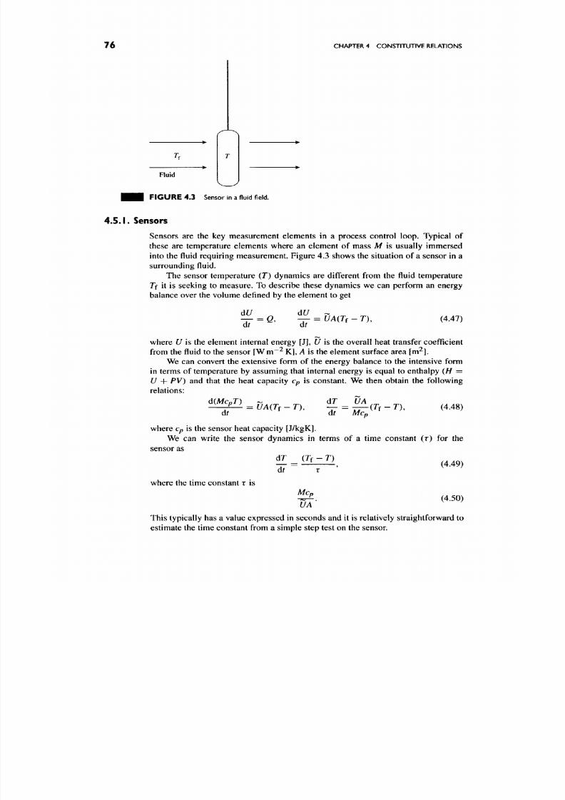
8/17/2019 Process Modelling and Model Analysis-Hangos-Cameron
http://slidepdf.com/reader/full/process-modelling-and-model-analysis-hangos-cameron 93/560
76
CHAPTER 4 CON STITUTIVE RELATIONS
Fluid
F IG U R E 4.3 Sensor in a fluid field.
4 . 5 . 1 .
Sensors
Sensors are the key measurement elements in a process control loop. Typical of
these are temperature elements where an element of mass M is usually immersed
into the fluid requiring measurement. Figure 4.3 shows the situation of a sensor in a
surrounding fluid.
The sensor temperature (T ) dynamics are different from the fluid temperature
Tf it is seeking to measure. To describe these dynamics we can perform an energy
balance over the volume defined by the element to get
dL^
dU -
(4.47)
where U is the element internal energy [J], U is the overall heat transfer coefficient
from the fluid to the sensor [Wm~^ K],
A
is the element surface area [m^].
We can convert the extensive form of the energy balance to the intensive form
in terms of temperature by assuming that internal energy is equal to enthalpy (H =
U
+
PV)
and that the heat capacity Cp is constant. We then obtain the following
relations:
-^
—
P-i = UA{Tf -
7) ,
dt
dT UA ^^ ^^
dr
Mc„
(4.48)
where Cp is the sensor heat capacity [J/kgK].
We can write the sensor dynamics in terms of a time constant (r) for the
sensor as
dr _ (rf - T)
dt ~ r '
where the time constant T is
(4.49)
Mcp
'uA
(4.50)
This typically has a value expressed in seconds and it is relatively straightforward to
estimate the time constant from a simple step test on the sensor.
8/17/2019 Process Modelling and Model Analysis-Hangos-Cameron
http://slidepdf.com/reader/full/process-modelling-and-model-analysis-hangos-cameron 94/560
EQUIPMENT AND CONTROL RELATIONS 7 7
It can be easily seen that the Laplace transform of
Eq.
(4.49) leads to
^7 =Z i I l I (4.51)
r
giving the sensor transfer function:
ns) 1
Tf(s) rs + 1
or a typical first-order response.
(4.52)
4.5.2.
Transmitters
Transmitters convert the sensor signal into a control signal for use by recorders,
indicators
or
controllers. Typically,
the
sensor signal
is in
millivolts,
a
pressure
dif
ferential value or other app ropriate unit. This is converted into an air pressure signal
(20-10 0 kPa) or current (4- 20 mA). Hence, in modelling these elements we need an
algebraic relation which describes the output signal as a function of the sensor signal.
This is dependent on the transmitter zero and its measurement span. In many cases,
this is simply a linear relationship:
Op
=
Op^^^(Ip-zo)G.
(4.53)
where
Op
is the output signal (e.g. mA ), Op^.^ the minimum transmitter output signal,
Ip
the input value (e.g. 200°C), zo the minimum input value (e.g. 100°C), G the
transmitter gain
((Op^^^
-
Op^J/span)
and
span
is
(/p^,,
-
zo).
In some cases, it is possible to allow a time lag by im posing a first-order response
as seen in the previous section.
4.5.3. Actuators
Control valve actuators respond to the controller output signal (/) and cause the valve
stem to be positioned to achieve a particular flow rate. These elements typically behave
as second-order systems of the form:
9
d^S dS
T^-jY+2HT— +S = Ga'I (4.54)
at"^ at
or as the second -order differential equation:
d r r X dt
where S is the stem m ovemen t (usually from 0 to 1), Ga the actuator gain and r and
^ are the time constant and damping factor for the actuator, respectively.
To solve this second-order OD E, we need to convert it to two first-order equations.
This
is
simply done
by
letting
dS
^ = w; (4.56)
dt
8/17/2019 Process Modelling and Model Analysis-Hangos-Cameron
http://slidepdf.com/reader/full/process-modelling-and-model-analysis-hangos-cameron 95/560
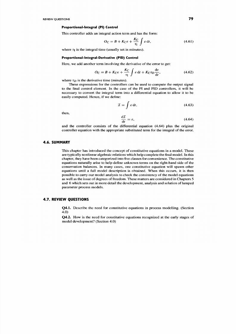
8/17/2019 Process Modelling and Model Analysis-Hangos-Cameron
http://slidepdf.com/reader/full/process-modelling-and-model-analysis-hangos-cameron 96/560
REVIEW QUESTIONS 79
Proportional-Integral (PI) Control
This controller adds an integral action term and has the form:
Oc=B-hKcs
+ — f ed t,
(4.61)
where rj is the integral time (usually set in minutes).
Proportional-lntegral-Derivative (PID) Control
Here, we add another term involving the derivative of the error to get:
Kr f d£
Oc=B-\-Kcs-\-— sdt + KcTD — , (4.62)
T\ J At
where TO is the derivative time (m inutes).
These expressions for the controllers can be used to compute the output signal
to the final control element. In the case of the PI and PID controllers, it will be
necessary to convert the integral term into a differential equation to allow it to be
easily computed. Hence, if we define:
- / '
sdt,
(4.63)
then,
d J
— = ^, (4.64)
at
and the controller consists of the differential equation (4.64) plus the original
controller equation with the appropriate substituted term for the integral of the error.
4.6.
SUMMARY
This chapter has introduced the concept of constitutive equations in a model. These
are typically nonlinear algebraic relations w hich help comp lete the final model. In this
chapter, they have been categorized into five classes for convenience. The constitutive
equations naturally arise to help define unknown terms on the right-hand side of the
conservation balances. In many cases, one constitutive equation will spawn other
equations until a full model description is obtained. When this occurs, it is then
possible to carry our model analysis to check the consistency of the model equations
as well as the issue of degrees of freedom. These m atters are considered in Chapters 5
and 6 which sets out in more detail the development, ana lysis and solution of lumped
parameter process models.
4.7.
REVIEW QUESTIONS
Q4.1. Desc ribe the need for constitutive equations in process mod elling. (Section
4.0)
Q4.2. How is the need for constitutive equations recognized at the early stages of
model development? (Section 4.0)
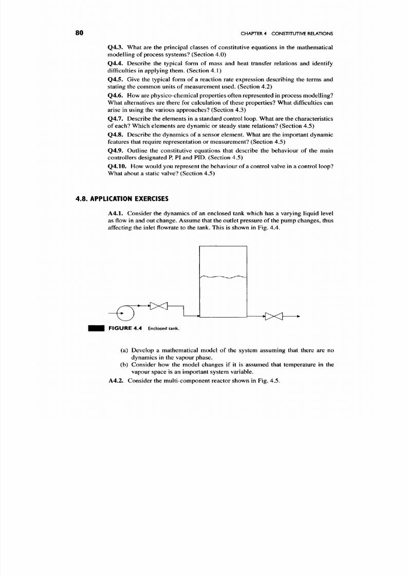
8/17/2019 Process Modelling and Model Analysis-Hangos-Cameron
http://slidepdf.com/reader/full/process-modelling-and-model-analysis-hangos-cameron 97/560
80
CHAPTER 4 CON STITUTIVE RELATIONS
Q4.3. What are the principal classes of constitutive equations in the mathematical
modelling
of
process systems? (Section 4.0)
Q4.4. Describe the typical form of mass and heat transfer relations and identify
difficulties
in
applying them. (Section 4.1)
Q4.5. Give the typical form of a reaction rate expression describing the terms and
stating the common units
of
measurement used. (Section 4.2)
Q4.6. How are physico-chem ical properties often represented in process mo delling?
What alternatives are there for calculation of these properties? Wh at difficulties can
arise in using the various approaches? (Section 4.3)
Q4.7. Describe the elements in a standard control loo p. What are the c haracteristics
of each? Which elements are dynamic
or
steady state relations? (Section 4.5)
Q4.8. Describe the dynamics of a sensor element. What are the important dynamic
features that require representation or measurement? (Section 4.5)
Q4.9.
Outline
the
constitutive equations that describe
the
behaviour
of the
main
controllers designated
P,
PI and PID. (Section 4.5)
Q4.10. How would you represent the behaviour of a control valve in a control loop?
What about
a
static valve? (Section 4.5)
4.8 .
APPLICATION EXERCISES
A4.1. Consider the dynamics
of
an enclosed tank which has
a
varying liquid level
as flow in and out chan ge. Assu me that the outlet pressure of the pump ch anges, thus
affecting the inlet flowrate to the tank. This
is
shown in Fig. 4.4.
-[xl
^-4x^
FIGURE 4.4 Enclosed tank.
(a) Develop a mathematical model of the system assuming that there are no
dynamics
in
the vapour p hase.
(b) Consider how the model changes if it is assumed that temperature in the
vapour space
is
an impo rtant system variable.
A4.2. Consider the multi-comp onent reactor shown in Fig. 4.5 .

8/17/2019 Process Modelling and Model Analysis-Hangos-Cameron
http://slidepdf.com/reader/full/process-modelling-and-model-analysis-hangos-cameron 98/560
APP LICATIO N EXERCISES
81
The CST R carries out a complex m ulti-component reaction sequence given by
A+B X,
B-^X^Y, B-\-Y-^Z. (4.65)
The reactions have rate constants of
k\
,
k2
and
k^.
(a) Given a fresh feed co nsisting of A and B, with inlet concentrations of
CAO^CBQ,
develop a mathematical model which describes the process
dynamics assuming that the reactor operates isothermally.
(b) If the reactions are exothermic with heat of reaction
A / / R ,
develop the model
for the non-isothermal case.
(c) Develop a further enhanc ement of the model wh ere a cooling w ater coil of
surface area
A
is inserted into the reactor to control the reactor temperature
to a nominated setpoint.
in-flow
O L < 0
out-flow
F I G U R E 4 .5 Continuous st irred tank reactor.
Spent gas
F I G U R E 4 .6 Oxidation reactor .

8/17/2019 Process Modelling and Model Analysis-Hangos-Cameron
http://slidepdf.com/reader/full/process-modelling-and-model-analysis-hangos-cameron 99/560
8/17/2019 Process Modelling and Model Analysis-Hangos-Cameron
http://slidepdf.com/reader/full/process-modelling-and-model-analysis-hangos-cameron 100/560
DYNAMIC MODELS—LUMPED
PARAMETER SYSTEMS
This chapter develops the underlying modelling principles for lumped parameter
systems (LPSs) and the subsequent analysis of those m odels. Here, we are concerned
about the time varying behaviour of systems w hich are considered to have states which
are homogeneous within the balance volume V. Hence, the concept of "lum ping" the
scalar
field
nto a representative single state value. Som etimes the term "well mixed" is
applied to such system s w here the spatial variation in the scalar field, which describes
the state of interest, is uniform. In some cases, we may also consider the stationary
behaviour of such systems which leads to steady state model descriptions.
In this section, the most general case is treated. Special emphasis is put on the
various forms of initial and boundary conditions that arise with their engineering
meaning as well as the effect of these conditions on the solution properties of the
process model.
Lumped parameter dynamic models, or compartmental models are widely used
for control and diagnos tic purpose s, these applications being considered in more detail
in Chapters 13 and 14. As well, they are frequendy used as the basis for engineering
design, startup and shutdown studies as well as assessing safe operating procedures.
5.1 .
CHARACTERIZING MODELS AND MODEL EQUATION SETS
As has been m entioned in Chapters 1 and 2, the modelling assumptions that are made
will lead to various dynamic and steady-state model forms.
83
8/17/2019 Process Modelling and Model Analysis-Hangos-Cameron
http://slidepdf.com/reader/full/process-modelling-and-model-analysis-hangos-cameron 101/560
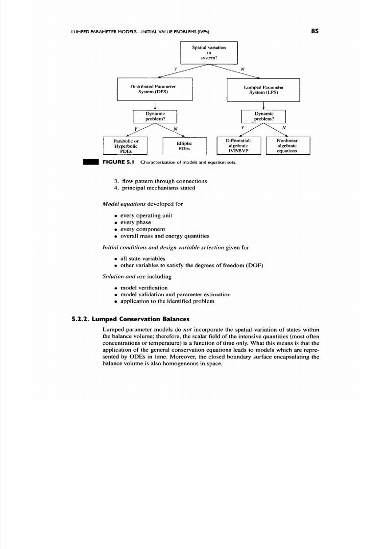
8/17/2019 Process Modelling and Model Analysis-Hangos-Cameron
http://slidepdf.com/reader/full/process-modelling-and-model-analysis-hangos-cameron 102/560
LUMPED PARAMETER MO DEL S—IN ITIAL VALUE PROBLEMS (IVPs) 85
Distributed Parameter
System (DPS)
Lumped Parameter
System (LPS)
y
Dynamic
problem?
Y
^ / \ .
N
Differential-
algebraic
IVP/BVP 1
Nonlinear
algebraic
equations
F I G U R E 5 .1 Chara cterization of models and equation sets.
3. flow pattern through connections
4. principal mechanisms stated
Model equations developed for
• every operating unit
• every phase
• every component
• overall mass and energy quantities
Initial conditions a nd design variable selection
given for
• all state variables
• other variables to satisfy the degrees of freedom (DO F)
Solution and use
including
• model verification
• mod el validation and param eter estimation
• application to the identified p roblem
5.2.2. Lumped Conservation Balances
Lumped parameter models do no t incorporate the spatial variation of states within
the balance volume; therefore, the scalar field of the intensive quantities (most often
conc entrations or temp erature) is a function of time only. What this mean s is that the
application of the general conservation equations leads to models which are repre
sented by ODEs in time. Moreover, the closed boundary surface encapsulating the
balance volume is also homogeneous in space.

8/17/2019 Process Modelling and Model Analysis-Hangos-Cameron
http://slidepdf.com/reader/full/process-modelling-and-model-analysis-hangos-cameron 103/560
86
CHAPTER 5 DYNAM IC MODELS—LUMPED PARAMETER SYSTEMS
Chapter
3
introduced the general conservation balance over a 3D volume V with
a closed boundary surface T and its integral (3.16) and differential (3.17) form. For
lumped parameter m odels we apply the integral form of
the
conservation balances
and use the condition of homogeneity of all variables in space. This enables us to
take the variables for the volume-specific extensive quantity (O) and its source
(q)
out from the volumetric integral terms in Eq. (3.16) as well as considering the flow J
as an overall flow through the whole surface
T
with no diffusive but only convective
and transfer flows present. In this case, J = Jc - Therefore, the general form of the
conservation b alances for a conserved extensive quantity 4) in the case of LPSs is as
follows:
do
^ = / c + . , (5.1)
with
Jc=4 -/ \
(5.2)
where J^ is the inflow and J^ is the outflow of the conserved extensive quan tity 4).
The following sections outline the basic conservation principles and c onstitutive
equation setup underlying lumped parameter model development.
5.3. CONSERVATION BAUNCES FOR MASS
Let us develop the general expressions for both
total and component mass balances
in a process system. Figure 5.2 shows a general balance volume for mass, given as
a defined space with boundary E ^ . Here, the comp onent flows into the system are
given
Sisfi
for component / in streamy, whilst the total stream flow is F ( = J^jf^ ).
Mass flows out of the system are shown
asf.
^ with total stream flows as F^.
Within the balance volume V we have the total component mass m/ (/ = , . . . , « )
and total mass M ( =
^ 1 /
^i)-
From the figure, we can identify that there are several ways mass can enter
and leave the balance volume through the boundary surface E ^ . In most cases , the
transfers are convective flows where material is entering and leaving the system via
stream flows, typically through p iped conn ections. The flows might also be associated
with diffusional mech anisms where m ass moves un der the influence of a potential or
Flows of mass in
//^^^^-^.^ / M \ Flows of
mass
out
F I G U R E 5 .2 General mass balance volum e.
8/17/2019 Process Modelling and Model Analysis-Hangos-Cameron
http://slidepdf.com/reader/full/process-modelling-and-model-analysis-hangos-cameron 104/560
8/17/2019 Process Modelling and Model Analysis-Hangos-Cameron
http://slidepdf.com/reader/full/process-modelling-and-model-analysis-hangos-cameron 105/560
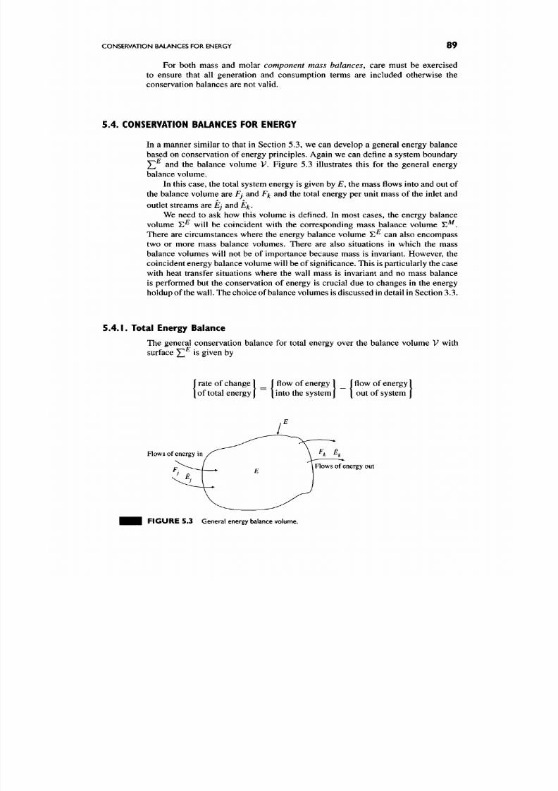
8/17/2019 Process Modelling and Model Analysis-Hangos-Cameron
http://slidepdf.com/reader/full/process-modelling-and-model-analysis-hangos-cameron 106/560
CONSERVATION BALANCES FOR ENERGY
89
For both mass and molar component mass balances, care must be exercised
to ensure that all generation and consumption terms are included otherwise the
conservation balances are not valid.
5 A CONSERVATION BALANCES FOR ENERGY
In a manner similar to that in Section 5.3, we can develop a general energy balance
based on conservation of energy principles. Again we can define a system boundary
Yf
and the balance volum e V. Figure 5.3 illustrates this for the general energy
balance volume.
In this case, the total system energy is given by £", the m ass flows into and out of
the balance volume are Fj and F^ and the total energy per unit mass of the inlet and
outlet streams are
E j
and
E^.
We need to ask how this volume is defined. In most cases, the energy balance
volume E ^ will be coincident with the corresponding mass balance volume S ^ .
There are circumstances where the energy balance volume E^ can also encompass
two or more mass balance volumes. There are also situations in which the mass
balance volumes will not be of importance because mass is invariant. However, the
coincident energy balance volum e will be of significance. T his is particularly the case
with heat transfer situations where the wall mass is invariant and no mass balance
is performed but the conservation of energy is crucial due to changes in the energy
holdu p of the wall. The ch oice of balance volumes is discussed in detail in Section 3.3.
5.4 .1 .
Total Energy Balance
The general conservation balance for total energy over the balance volume V with
surface ^ ^ is given by
rate of change |
of total energ y]
flow of energy | _ fflow of energy
into the system J | out of system
How s of energy in
F.. 6^
Flows of energy out
F I G U R E 5 . 3 General energy balance volume.
8/17/2019 Process Modelling and Model Analysis-Hangos-Cameron
http://slidepdf.com/reader/full/process-modelling-and-model-analysis-hangos-cameron 107/560
90
CHAPTER 5 DYN AMIC MODELS—LUMPED PARAMETER SYSTEMS
The total energy
E
[J] of
the
system comprises three principal com ponents in process
systems:
• internal energy
U
• kinetic energy
KE
•
potential energy
PE
Hence, we can write
E = U-\-KE-\-PE^
(5.10)
It is necessary to define in what ways energy flows into and out of the system.
We consider the principal components of these energy flows as
• convective energy flows
• conductive and radiative heat flows
• work terms
Convective Energy Flows
These are associated with the energy carried by each mass flow
F j
and
F ^
ir^to and
out of the balance volume. We associate with each mass flow an energy flow which
is made up of internal, kinetic and potential energy. Thus the convective energy flows
can b e written for inlet and outlet flows as
P
Y^Fj{U
+ kE + PE)j
(5.11)
7 = 1
and
Y,W +
kE-\-PE)k.
(5.12)
k=l
where U, KE, PE are specific energy quantities. Typically, they are defined as energy
per unit mass [J/kg]. They can also be written in molar units [J/mol] and designated
as U, KE and PE-
Conductive and Radiative Heat Flows
These are given as follows:
• Conductive energy w hich flows either in or out of the system through con
ductive heat transfer m echanism s associated w ith the interfaces of the balance
volume. We can designate these as
Qc-
• Radiative energy flows either in or out of the system through radiation heat
transfer mechanisms, given by
QR.
The two previous categories of energy flows are conventionally combined
together and written as
G = Gc + eR . (5.13)
8/17/2019 Process Modelling and Model Analysis-Hangos-Cameron
http://slidepdf.com/reader/full/process-modelling-and-model-analysis-hangos-cameron 108/560
CONSERVA TION BALANCES FOR ENERGY 9 1
Work Terms
The energy balance m ay contain terms describing the work do ne by the system on the
surrounding s w hich consists of several terms. We note that the accepted convention is
that work done on the system is regarded as positive work. The wo rk terms of interest
are now discussed:
• Shaft work (Ws) which accounts for mechanical energy flow to or from the
system. Shaft work done on the system by the surroundings raises the energy
content of the system and is thus positive work.
• Expansion work (WE) which accounts for work done in expansion or contrac
tion of the balance vo lume. This term is often not present especially w hen the
balance volume is fixed such as in the case of a piece of process equipment.
However, in many circumstances where balance volumes share an interface
and the interface is movable then this term can be important.
Where the
sysiempressure
remains
constant,
the expansion work
is
related
to the force applied on the boundary and the rate of boundary movem ent giving:
dV
WE = - P — , (5.14)
at
where
pressure is not constant
over the boundary, it is necessary to carry out a
volumetric integral over the volume V to com pute the expansion work given by
L
E = - P( r , r )d v. (5.15)
Iv
•
Flow w ork (Wp) which relates to work done on the fluid as it moves into and
out of the balance volume. This depends on the inlet and outlet pressures, the
specific volumes of the fluids at these conditions and the mass flows of the
streams. This flow work contribution on the system can be expressed as
p q
^¥ = Y.
^i(^^)i - E
f'k{py)k
(5.16)
The Total Energy Balance
The conservation balance for energy over the balance volume V can now be written as
— = ^ F j E j -Y^Fuh- \-Q+ W. (5.17)
j=\ k=\
We can expand the work quantity to obtain
Ar P q
-77 = J2^J^^-^^E+PE )j-J2^f^^^-^^E-^PE )k-^Q (5.18)
^^ j=\ k=\
+
q
j=l k=\
(5.19)

8/17/2019 Process Modelling and Model Analysis-Hangos-Cameron
http://slidepdf.com/reader/full/process-modelling-and-model-analysis-hangos-cameron 109/560
92 CHAPTER 5 DYNAMIC MODELS—LUMPED PARAMETER SYSTEMS
and after rearrangement we get
dE ^
— = J2 ^J^ + Py + KE-\- P E ) J (5.20)
J2Fk{u-\-pv-\-kE + PE )k-^Q-^'^^
where W = WE-\- WS.
Using the thermodynamic relationship for enthalpy
H
given
by H = U -{- P V,
it
is possible to write the general energy balance using m ass specific enthalpy
H
[J/kg]
as
— = J2Pj(ff-^^E -^PE )j-J2^f^^^-^^E-\ -PE)k +
Q
+
W .
(5.21)
The general energy balance equation (5.21) can also be written in equivalent
molar terms, using
H
to represent stream enthalpy per unit mole. Other terms in the
equation are similarly defined in molar units.
It should
also
be noted that Eq. (5.21) contains implicitly any energy contributions
from internal processes, specifically those associated with chemical reactions. The
next section will develop a nu mber of key simplifications of the general energy balanc e
which are applicable for a range of common process engineering applications.
5.4.2. Simplifications and Modifications of the General Energy Balance
In many process systems applications, we can make a number of simplifications to
the terms shown in Eq. (5.21). We now review some of these:
Assumption 1 In many cases, the kinetic and potential energy comp onents can be
neglected:
• KE — 0, since many flows are low velocity and the energy contribution of the
term
(FjV^/2)
is small.
• PE — 0 , since elevation differences for many process systems are small and
hence the energy contribution (Fyz,
z =
elevation) is small.
These simplifications lead to a final simplified form of the energy balance where
the right-hand side terms are now w ritten in terms of specific enthalpies. The left-hand
side represents the total internal energy of the system . This is a common representation
in chemical process systems where internal energy content often dominates the total
energy content of the system.
AJJ P ^
-^ = T.^A -T.^kHk + e + iV. ( 5 . 2 2 )
Com putation of the specific enthalpies for all inlet and outlet streams is usually done
using thermodynamic prediction packages which can take into account fluid phase
8/17/2019 Process Modelling and Model Analysis-Hangos-Cameron
http://slidepdf.com/reader/full/process-modelling-and-model-analysis-hangos-cameron 110/560
CONSERVATION BALANCES FOR ENERGY
93
non-idealities. Other simplifications of the enthalpy representation can also be made
as seen in Section 4.3.
Assumption 2 We normally do not deal directly with the internal energy
U,
in the
general energy balanc e such as Eq. (5.22) but prefer to use alternate properties. U sing
the definition of enthalpy we can write Eq. (5.22) as
— = - ^^— l = J2FjHj-J^F,Hk-^Q^W , ( 5 . 2 3 )
'i-'- -t A-t'' ^
+ Q+^-
( 5 . 2 4 )
7=1 k=\
If P and V are constant, then we can write,
dH ^ ^
j=\ k=l
This is often not the case in gas phase systems.
Assumption 3 In Eq. (5.25), the specific enthalpy of the balance volume and the
specific enthalpy at the outlet are not necessarily equal. In the case where pres
sure variations within the balance volume are small, such as in liquid systems or
where enthalpy variations due to pressure are small, we can assume that the specific
enthalpies are equal and hence:
H = Hk k=h,. .,q.
(5.26)
We can then write the energy balance as
-^=J1 ^A -J2''lcH
+ Q+W. ( 5 . 2 7 )
; = 1 ^ = 1
This is the most com mon form of the energy balance for a liquid system .
Assumption 4 We know that in Eq. (5 .27), the enthalpies are evaluated at the
temperature conditions of the feeds (7)) and also at the system temperature
(T).
By
making certain assumptions about the enthalpy representation, we can make further
simplifications. In particular, we note that the enthalpy of the feed Hj can be written
in terms of the system temperature
T.
Hj(Tj) = Hj(T)-^j
Cp.{T)dT. (5.28)
If we assume that
C p
is a constant, then
Hj{Tj) = Hj(T)
+ CpjiTj
- T).
(5.29)
8/17/2019 Process Modelling and Model Analysis-Hangos-Cameron
http://slidepdf.com/reader/full/process-modelling-and-model-analysis-hangos-cameron 111/560
94
CHAPTER 5 DYN AMIC MODELS—LUMPED PARAMETER SYSTEMS
Hence, we can write our modified energy balance as
dH ^ r 1 ^
-J7 = Il^j\^i(^) + ^PJ^'^J - ^> - E ^ k H ( T ) + e + W. (5.30)
"^
j=\ k=\
In this case, the first term is the energy contribution needed to adjust the feed enthalpy
at its inlet conditions to the conditions of the balance volum e.
Assumption 5 It has already been mentioned that when considering reacting sys
tems no explicit appearance of the heat of reaction is seen in the general energy
balance. This is because the energy gain or loss is seen in the value of the outlet
enthalpy evaluated at the system temperature T. We can now develop the energy
balance in a way which makes the reaction term explicit in the energy balance.
We first note that enthalpy is a function of temperature, pressure and the m oles
of species, /i/, / = 1 , . . . , nc giving
H =f(T,
P , n/) and hence the time derivative of
this relationship is given by
d//
dHdT dHdP .^dHdrii
— = + f-> -. (5.31)
dt dT dt dP dt ^
drii
dt ^ ^
Here, the term dH/dni is the partial molar enthalpy of species /, which we can
write as
Hi.
Now, in the case of liquid systems, the term dH/dP is close to zero and is
identically zero for ideal gases. We can also note that the definition of specific heat
per unit mass at constant pressure is given by
[dTj
(5.32)
p
This then allows us to write the general equation (5.31) as
d / / ^T
j - ^ -
dtti
I
The last term in Eq. (5.33) can be expanded using the mass balances for a reacting
system wh ere the species n/ appear or are consumed. For a general reaction given by
vx X -{- vyY -^ vwW -^ vzZ,
(5.34)
we can write the species mole balances given by Eq. (5.5) as
dn ^ - ^ -
-d7 = E ^ V - E ^ ^ ^ + '^^'
i=^^'^nc,
(5.35)
The last term in Eq. (5.33) then becomes
nc t nc p nc q nc
E ^ ' ^ =
E ^ ' E A > - E ^ ' E A .
+
^^E^'-'- 5 . 3 6 )
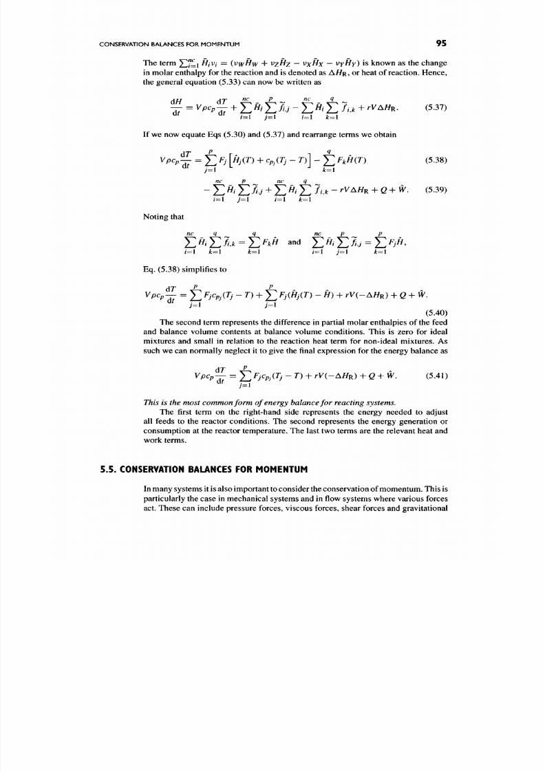
8/17/2019 Process Modelling and Model Analysis-Hangos-Cameron
http://slidepdf.com/reader/full/process-modelling-and-model-analysis-hangos-cameron 112/560
CONSERVATION BALANCES FOR MOMENTUM 95
The term X]?=i ^i^i — iVwfiw
+
^z^iz — ^xHx — ^yHy)
is
known
as the
change
in molar enthalpy
for
the reaction
and is
denoted
as
A / / R ,
or
heat
of
reaction. Hence,
the general equation (5.33)
can now be
written
as
dH
dT ^^ ^ nc _ q
•dT ^^' d7
"
"' ^
-
- E ^' E / a +
'• ' R-
(5.37)
i=\
j={ i=\ k—\
If we now equate Eqs (5.30) and (5.37) and rearrange terms we obtain
dr
^ r
1 ^
^P'P-^
= E
^J
ri (^) +
^PJ^^J
- )J
-H^kHiT) (5.38)
7= 1
k=\
nc p nc q
-J2"iJl h -^H^iJl
fi^k
- rVAHK
+
Q-hW,
(5.39)
i=z\ j=\ i=\ k=\
Noting that
nc q q nc p p
T.^iJ2fik = E^kH
and
E^'EAy =
E ^ A
/= 1 k=l k=\ i=\ j=\ k=\
Eq. (5.38) simplifies to
AJ
P P
^^"^pi;
= J2^j''pj^^j
- ^) + E^i(^^(^) ~ ) + rV{-AHK) + e +w .
(5.40)
The second term represents the difference in partial molar enthalpies of the feed
and balance volume contents
at
balance volume conditions. This
is
zero
for
ideal
mixtures and small in relation to the reaction heat term for non-ideal mixtures. As
such we can normally neglect it to give the final expression for the energy balance as
dr
^
' ^P d7
= E ^J^PA^J -
>
+ ' •^(-^^R) + G + W.
(5.41)
7=1
This is the most common form of energy balance for reacting systems.
The first term
on the
right-hand side represents
the
energy needed
to
adjust
all feeds to the reactor conditions. The second represents the energy generation or
consumption at the reactor temperature. The last two terms are the relevant heat and
work terms.
5.5. CONSERVATION BALANCES FOR MOMENTUM
In many systems it
is
also important
to
consider the conservation of momentum. This is
particularly the case in mechanical systems and in flow systems where various forces
act. These can include pressure forces, viscous forces, shear forces and gravitational
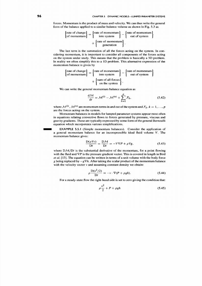
8/17/2019 Process Modelling and Model Analysis-Hangos-Cameron
http://slidepdf.com/reader/full/process-modelling-and-model-analysis-hangos-cameron 113/560
96
CHAPTER 5 DYN AMIC MODELS—LUMPED PARAMETER SYSTEMS
forces. M omentum is the product of mass and velocity. We can thus w rite the general
form of the balance applied to a similar balance volume as shown in Fig. 5.3 as
rate of change 1 _ f rate of mom entum 1 f rate of mom entum 1
of momentum
J
~ | into system j | out of system J
I rate of momentum
I generation J
*
The last term is the summation of all the forces acting on the system. In con
sidering momentum, it is important to consider all components of the forces acting
on the system under study. This means that the problem is basically a 3D problem.
In reality we often simplify this to a ID problem. This alternative expression of the
momentum balance is given by
{
rate of change 1 _ |ra te of mom entum _ f rate of mom entum
of momentum J ~ | into system j | out of system J
f
sum of all forces
[ on the system J
*
We can write the general momentum balance equation as
^ = A ^ ( i ) - > l « » + ^ j r , , (5.42)
where M^^\M ^^ are momentum terms in and out of the system and
T^.k—
1 , . . . ,
/?
are the forces acting on the system.
Mom entum balances in models for lumped parameter systems appear most often
in equations relating convective flows to forces generated by pressure, viscous and
gravity gradients. These are typically expressed
by
some form of the general Bernoulli
equation which incorporates various simplifications.
EXAMPLE 5.5.1 (Simple mom entum balanc es). Consider the application of
a general momentum balance for an incompressible ideal fluid volume V. The
momentum balance gives:
D(pVv) DM
J ^ . _ _ = _ V V P + , V , , (5.43)
where DAI/Dr is the substantial derivative of the momentum, for a point flowing
with the fluid and V P is the pressure gradient vector. This is covered in length in Bird
et
al.
[13]. The equation can be w ritten in terms of a unit volume w ith the body force
g
being replaced by
— g^h .
After taking the scalar product of the momentum balance
with the velocity vector v and assuming constant density we obtain:
D(v2/2)
P — ^
= -^ '
^ ( ^ +
P8hl
(5.44)
For a steady-state flow the right-hand side is set to zero giving the condition that:
Pj + P + pgh
(5.45)

8/17/2019 Process Modelling and Model Analysis-Hangos-Cameron
http://slidepdf.com/reader/full/process-modelling-and-model-analysis-hangos-cameron 114/560
CONSERVATION BALANCES FOR M OME NTUM
97
should be constant. This is the well-known static Bernoulli momentum balance
without the presence of viscous forces producing friction losses in the flow.
Equation (5.45) is often used for modelling flows in piping systems and through
valves. A particular form of the equation leads to a simple steady-state constitutive
equation for the flow through a valve as
F = CyVXP, (5.46)
where Cy is the valve coefficient.
Momentum balances also have an important role in modelling of mechanical
system where various forces are at work. One of the simplest examples of this is the
dynamics of a control valve actuator and stem, as shown in the following example.
EXAMPLE 5.5.2 (The dynam ics of a control valve). Con sider the actuator and
stem of a control valve shown in Fig. 5.4. The diaphragm moves the stem position
x
a t
a velocity v, under the force exerted by ch anging the air pressure P on the diaphragm.
This is resisted by a spring and the friction associated w ith the stem m oving through
the packing. A mo mentum balance can be carried out of the stem assembly of mass
M noting that there are three principal forces at work. These are the force on the
diaphragm due to air pressure (Fj), the compression force exerted by the spring (Fs)
and frictional forces due to the stem packing (Fp).
The momentum balance gives
(5.47)
M
d(Mv)
Substituting for the forces, we have
dv
M — = P A
—
kx
—
cv,
at
r^^^^
^Hi
^ m
/]
1 1 diaphragm area, A
1 stem velocity, V
[ ^ stem packing
r~^
(5.48)
plug and seat
F IG U R E 5 .4 Control valve actuator and stem.

8/17/2019 Process Modelling and Model Analysis-Hangos-Cameron
http://slidepdf.com/reader/full/process-modelling-and-model-analysis-hangos-cameron 115/560
98
CHAPTER 5 DYNAMIC MODELS—LUMPED PARAMETER SYSTEMS
where k is the spring constant and c is a coefficient of friction for the packing. Final
rearrangement of the equation leads to
/ M \ d^jc / c \ dx /PA\
which is a form of a second-order system response given by
' id jc dx
r ^ - — + 2 § T — + j c = ^ (5 .5 0)
dr2 ^ dr
• • • with r = y/W Jk and
^
=
\/2^(c^/(kM)),
5.6.
TH E SET OF
CONSERVATION BALANCES
FOR
LUMPED SYSTEMS
The proces s model of an LPS c onsists of a set of conservation balance equations that
are ODEs equipped with suitable constitutive equations. The balance equations are
usually coupled through reaction rate and transfer terms. This is illustrated on the
following example of a CSTR which can be seen as a modelling unit of all lumped
parameter system models.
• • 1 EXAMPLE 5.6.1 (Lumped parameter modelling of a CST R).
A CSTR is shown in Fig. 5.5 with reactant volume V, component mass holdup m^
for com ponent
A,
feed flowrate F^*^ [m^/s] at temperature
T^^\
Feed concentration
of component/4 is c^ . Outlet flowrate
F^^^
is in units
[m^/s].
Assumptions
Al. perfect mixing implying no spatial variations,
A2.
incompressible fluid phase ,
A3, constant physical properties,
A4. all flows and properties given in mole units,
^ 5 . equal molar densities,
A6.
reactions and reaction rates given by
A - > P ,
rA=ko^-^^^^^^CA.
(5.51)
Model
equations
First, we set up the model equations in their extensive form written in molar quantities.
The following state the
overall ma ss balance, the
component
balance for A and the
total energy balance.
accumulation-rate = in-flow — out-flow 4- source,
djpV)
dt
d(mA) Ai) Ao) .,„ ^^- ^^
dt
Vpcp —
= F<*>;o<'> - F ( ° > p ,
_
At) Ao)
-JA ~JA
= F W W < ' V - F^^Hp
-VrA,
- VrAAHR.

8/17/2019 Process Modelling and Model Analysis-Hangos-Cameron
http://slidepdf.com/reader/full/process-modelling-and-model-analysis-hangos-cameron 116/560
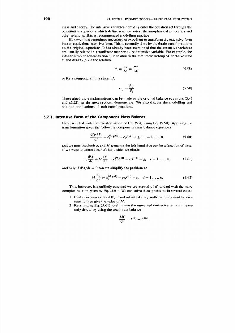
8/17/2019 Process Modelling and Model Analysis-Hangos-Cameron
http://slidepdf.com/reader/full/process-modelling-and-model-analysis-hangos-cameron 117/560
100
CHAPTER 5 DYN AMIC MODELS—LUMPED PARAMETER SYSTEMS
mass and energy. The intensive variables normally enter the equation set through the
constitutive equations which define reaction rates, thermo-physical properties and
other relations. This is recommended modelling practice.
However, it is sometimes necessary or expedient to transform the extensive form
into an equivalent intensive form. This is normally do ne by algebraic transformations
on the original equations. It has already been mentioned that the extensive variables
are usually related in a nonlinear manner to the intensive variable. For example, the
intensive molar concentration c/ is related to the total mass holdup M or the volume
V and density p via the relation
Q = 77 = -TT (5.58)
M pV
or for a component / in a streamy,
c / , ; - ^ . (5.59)
These algebraic transformations can be made on the original balance equations (5.4)
and (5.22), as the next sections demonstrate. We also discuss the modelling and
solution implications of such transformations.
5.7 .1 .
Intensive Form of the Component Mass Balance
Here, we deal with the transformation of Eq. (5.4) using Eq. (5.58). Applying the
transformation gives the following component mass balance equations:
^^=^^F^^-CiF^^^+gi i=X
« , (5.60)
at
and w e note that both c/ and M term s on the left-hand side can be a function of time.
If we were to expand the left-hand side, we obtain
c , ^ + M ^ = c f V « - c , F < ° ) + g , - I - , . . . . « . (5.61)
at at
and only if dM/dr = 0 can we simplify the problem as
M ^ = c f V ( * > - c / F ( « > + g / / = l , . . . , n . (5.62)
This, however, is a unlikely case and w e are normally left to deal with the m ore
complex relation given by Eq. (5.61). We can solve these problems in several ways:
1.
Find an expression for
dM/dt
and solve that along with the comp onent balance
equations to give the value of M.
2.
Rearranging E q. (5.61) to eliminate the unwanted derivative term and leave
only dc//dr by using the total mass balance
dt
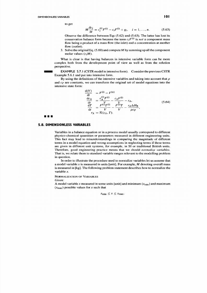
8/17/2019 Process Modelling and Model Analysis-Hangos-Cameron
http://slidepdf.com/reader/full/process-modelling-and-model-analysis-hangos-cameron 118/560
DIMENSIONLESS VARIABLES 1 0 1
to get
M ^ = c f V ^i) -
aF^'^ +gu
/ = , . . . ,
n,
(5.63)
at
Observe the difference between Eqs (5.62) and (5.63). The latter has lost its
conservation balance form because the term c/F^*^ is not a component mass
flow b eing a produ ct of a mass flow (the inlet) and a conc entration at ano ther
flow (outlet).
3. Solve the original Eq . (5.60) and com pute M by summing up all the component
molar values
{ciM).
What is clear is that having balances in intensive variable form can be more
complex both from the development point of view as well as from the solution
perspective.
• • • EXAMPLE 5.7.1 (CSTR model in intensive form). Consider the previous CSTR
Example 5.6.1 and put into intensive form.
By using the definitions of the intensive variables and taking into account that p
and cp are constants, we can transform the original set of model equations into the
intensive state form:
^ = / r ( i ) _ / 7 ( o )
dt ~ V V ''^' (5.64)
d7 ~ V V pep '
M
=n{cA.T).
5.8. DIMENSIONLESS VARIABLES
Variables in a balance equation or in a process m odel usually correspo nd to different
physico-chemical quantities or parameters measured in different engineering units.
This fact may lead to misunderstandings in comparing the magnitude of different
terms in a model equation and wrong assumptions in neglecting terms if these terms
are given in different unit systems, for example, in SI or traditional British units.
Therefore, good engineering practice means that we should
normalize variables.
That is, we relate them to standard variable ranges relevant to the mod elling pro blem
in question.
In order to illustrate the procedu re used to norm alize variables let us assume that
a model variable
x
is measured in units [unit]. For example,
M
denoting overall mass
is measured in
[kg].
The following p roblem statemen t describes how to normalize the
variable
x.
NORMALIZATION OF VARIABLES
Given:
A
model variable
x
m easured in some units [unit] and minimum (jc^in) and maxim um
(• max)
possible values for
jc
such that

8/17/2019 Process Modelling and Model Analysis-Hangos-Cameron
http://slidepdf.com/reader/full/process-modelling-and-model-analysis-hangos-cameron 119/560
102
CHAPTER 5 DYN AMIC MODELS—LUMPED PARAMETER SYSTEMS
Compute:
The normalized variable
Jc,
where
X =
It is easy to see, that the normalized variable x has the following advantageous
properties:
• its range is norm alized, i.e.
0 < j c < 1 ;
• it is unitless (dimen sionless).
The procedure can also be applied to the time variable so that time is also
normalized between 0 and 1.
Unitless or dimensionless model equations are those where all variables and
parameters are normalized. In doing this all variables are seen to be between 0 and
1.
Certain variables can also be grouped together leading to dimensionless numbers.
Many are well known such as Reynolds and Froude numbers. Others arise from the
application of the normalizing principle to different application areas such as reac
tion engineering where Biot and Damkohler numbers are important. Dimensionless
numbers also play a major part in the correlation of experimental data.
5.9. NORMALIZATION OF BALANCE EQUATIONS
The normalization of balance equations uses the techniques outlined in the previous
section and applies the procedure to all conserved quantities. In order to illustrate
the technique and some of the important outcomes, we consider Example 5.7.1,
which gives both mass and energy balance equations for a reaction in a continuous
stirred tank.
The mass balance equation can be written in intensive form as
V^=F ^icf-CA)-rV, (5.65)
where
V
was the volume of reactants
[m^],
F^' was the volumetric flowrate [m^
s~^],
r was the reaction rate [mol • s~^
•
m^], c^ was the feed concentration [mol
•
m~ ^] ,
and CA was the concentration in the reactor [mol • m~^ ] .
We can easily rearrange this equation by dividing through by the volume V, to
give
dcA F^^icf -CA)
or
- r, (5.67)
cA __ {C A - (^A)
At T
where T has the units of [s], being a characteristic time constant for the reactor.

8/17/2019 Process Modelling and Model Analysis-Hangos-Cameron
http://slidepdf.com/reader/full/process-modelling-and-model-analysis-hangos-cameron 120/560
8/17/2019 Process Modelling and Model Analysis-Hangos-Cameron
http://slidepdf.com/reader/full/process-modelling-and-model-analysis-hangos-cameron 121/560
I 04
CHAPTER 5 DYN AMI C MODELS—LUMPED PARAMETER SYSTEMS
Steady-State energy balance
P
0 = Y^Fj{U-hPiVi+kE +
PE)j
(5.74)
q
k=\
These equations are typically solved using some form of iterative numerical
solver such as New ton's m ethod or a variant. Steady-state balances form the basis for
the substantial number of process flowsheeting programs which are routinely used in
the process industries. These include ASP EN PLU S [30], HYS IM [31] and PRO II.
5.11.
ANALYSIS OF LUMPED PARAMETER MODELS
5 .1 1 .L Degrees of Freedom Analysis
In the same way that algebraic equations require a degree of freedom analysis to
ensure they are properly posed and solvable, dynamic models also require a similar
analysis.
The basis concept of DOF analysis is to determine the difference between the
number of variables (unknowns) in a given problem, and the number of equations
that describe a mathematical representation of the problem.
Thus,
where A^DF is the number of DOF, TVu the number of independent variables (unknow ns)
and
A e
the number of independent equations.
There are three possible values for A^DF to take:
(a) A DF = 0- Th is im plies that the num ber of ind epend ent unknowns and
independent equations is the same.
A
unique
solution may exist.
(b) A DF > 0- This implies that the num ber of independent variables is greater than
the number of independent equations.
The problem is
underspecified
and a solution is possible only if some
of the independent variables are "fixed" (i.e. held constant) by some external
considerations in order that
A^DF
be reduced to zero. Some thought must be
given to which system variables are chosen as fixed. In the case of o ptimization
these DO F will be adjusted to give a "best" so lution to the prob lem.
(c) A DF < 0- This im plies that the num ber of variables is less than the num ber of
equations.
The problem is overspecified, meaning that there are less variables than
equations. If this occurs it is necessary to check and make sure that you have
included all relevant equations. If so, then the solution to such a problem is
one which best "fits" all the equations. This is often called a "least squares"
solution.

8/17/2019 Process Modelling and Model Analysis-Hangos-Cameron
http://slidepdf.com/reader/full/process-modelling-and-model-analysis-hangos-cameron 122/560
ANALYSIS OF LUMPED PARAMETER MODELS
105
When calculating the DO F for a process model, there are several schemes which
can be used to count the variables and associated equation s. The key is to be consistent
with your approach.
Variables in the Model
Typical variables in the model have already been discussed in the previous sections.
As well as the variables there are parameters and constants which also appear. These
parameters are normally fixed by the designer but they can also be varied in order
to optimize the process system. They could be included in the DOF analysis for
completeness. In the section that follows we can develop our analysis using both
approa ches. We should get the same result The constants in the model equations are
not normally alerted and as such should not be included in the DOF analysis.
Equations in the Model
All equations must be independent. For example, one common mistake in writing
mass balanc es is to write the individual componen t balances
as well
as the overall mass
balance. These are dependent since the sum of the individual component balances
gives the overall mass balance.
Initial Conditions for Dynamic Models
It is important that the initial condition of al l the differential variables is set by the
user before any attempt is made to solve the problem. The initial conditions should
not be included as part of the DO F analysis but should be assum ed as essential to the
correct establishment of the model.
We will see that there are circumstances which arise where it is not possible to
independently select the initial condition for each state.
Selecting Variables to Satisfy the Degrees of Freedom
In many situations you will not be free to select just any variable you please as a
specified or design variable. In larger systems which are composed of a number of
components or processing units, it is not valid to overspecify one unit and leave
another underspecified so that the global DOF is satisfied. Hence, it is important to
check that in large problems, the subsystems are not overspecified.
Lumped parameter models generally take the form (semi-explicit):
^=f(y.zj), (5.75)
at
0 = g(y,zj).
(5.76)
w h er ej is the vector ofdifferential or state variables,
[y\,
j2» • • . , j n ]^ and
z
the vector
of algebraic variables (auxiliary variables), [z\, Z2» • •»
Zq]^.
f and g are general
nonlinear functions.
Here, we have n differential (state) equations and m algebraic eq uations, where
n
= dim/ and
m =
dim
g.
All up we have
n-\-m
independent equations.

8/17/2019 Process Modelling and Model Analysis-Hangos-Cameron
http://slidepdf.com/reader/full/process-modelling-and-model-analysis-hangos-cameron 123/560
I 06 CHAPTER 5 DYN AMIC MODELS—LUMPED PARAMETER SYSTEMS
The number of independent equations is then:
Ne = dimf + dimg,
(5.77)
where di m /
is
the number of independent differential equations and dim
g
the number
of independent algebraic equations. It is normally the case that we have
n
states in
our system with q auxiliary or algebraic variables (q > n).
Therefore, the number of DOF in this case is
A DP = n
-\-
q
—
d i m /
—
dim
g
(5.78)
Consequently, i f / /DF > 0, one has to specify
n-\-q
—
d i m / — dim
g
(5.79)
variables before any attempt can be made to solve the problem. The variables that
are selected to be specified before solving the dynamic model are often called design
variables or simply
specified
variables.
EXAMPLE 5.11.1 (A
simple tank model).
Con sider a simple tank model shown
in
Fig.
5.6. Here, we want
to
check how the DOF requirement
is
satisfied with different
specifications.
The process can be described by the following four equations:
dh
1
:(Fi-F2),
dt A
F\ - Cyy/Pi - P2 = 0,
Fi - Cyy/P2 - P3 = 0,
P2-Po-P8h = 0.
(f\)
(gl)
(82)
(83)
^
F,
• t x A
F I G U R E 5.6 Simple tank problem.
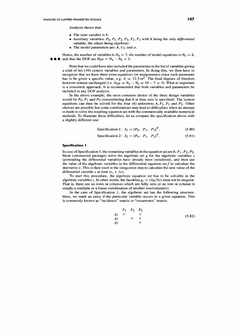
8/17/2019 Process Modelling and Model Analysis-Hangos-Cameron
http://slidepdf.com/reader/full/process-modelling-and-model-analysis-hangos-cameron 124/560
ANALYSIS OF LUMPED PARAMETER MODELS
107
Analysis shows that:
• The state variable is h.
• Auxiliary variables:
P{^,P\,P2,P^,F\,
F2 with
h
being the only
differential
variable, the others being
algebraic.
• The model parameters are: A, Cy and
p.
Hence, the number of variables is N^ = 7, the number of model equations is
A e
= 4»
• • • and thus the DO F are
N DF = Nu-Ne = 3.
Note that w e could have also included the parameters in the list of variables giving
a total of ten (10) system variables and parameters. In doing this, we then have to
recognize that we have three extra equations (or assignments) since each parameter
has to be given a specific value, e.g.
A =
12.5 m^. T he final degrees of freedom
however remain unchanged (i.e.
A^DF
= Ny^
—
NQ = 10
—
1 = 3). What is important
is a consistent approach. It is recommended that both variables and parameters be
included in any D OF analysis.
In the above example, the most common choice of the three design variables
would be PQ, P\ and P3 (remembering that h at time zero is specified). The system
equations can then be solved for the four (4) unknowns h, F\, F2 and P2. Other
choices are possible but som e combinations may lead to difficulties when an attempt
is made to solve the resulting equation set with the comm ercially available num erical
methods. To illustrate these difficulties, let us compare the specification above with
a slightly different one:
Specificat ion :
Si=[Po, Pu P^f.
(5.80)
Specification 2: ^2 = [^0, Fu Plf • (5.81)
Specification I
In case of Specification 1, the remaining variables in the equation set are A, F i , F2, P2-
Most commercial packages solve the algebraic set
g
for the algebraic variables
z
(pretending the differential variables have already been initialized), and then use
the value of the algebraic variables in the differential equation set/ to calculate the
derivative x. This is then used in the integration step to calculate the new value of the
differential variable
x
at time
(to
4-
At).
To start this procedure, the algebraic equation set has to be solvable in the
algebraic variables z. In other word s, the Jacobian
gz
= (dg/dz) must not be singular.
That is, there are no rows or columns which are fully zero or no row or column is
simply a multiple or a linear combination of another row/column(s).
In the case of Specification 1, the algebraic set has the following structure.
Here, we mark an entry if the particular variable occurs in a given equation. This
is commonly known as "incidence" m atrix or "occurrenc e" matrix.
Fi F2 F2
^1 ^ ^ (5.82)
g2 X X
^3 X

8/17/2019 Process Modelling and Model Analysis-Hangos-Cameron
http://slidepdf.com/reader/full/process-modelling-and-model-analysis-hangos-cameron 125/560
I 08 CHAPTER 5 DYNAMIC MODELS—LUMPED PARAMETER SYSTEMS
The above occurrence matrix shows that the Jacobian is non-singular. O bviously,
(^3) can be solved for P2, {g2) for F2 and {g\) for F\.
This specification is consistent and leads to "smooth" solution procedures. The
initial value of h can be given arbitrarily.
Specification 2
Specification 2, however, leads to some difficulties if we try to apply the same
procedure to solve the resulting equation set.
The first problem is encountered when we try to solve the algebraic equation
set for the algebraic variables. Although we specified the value of independent vari
ables and the degrees of freedom requirement was satisfied, g is not solvable in the
remaining algebraic variables We can see this from the occurrence matrix given by
F\ Fi P3
^^ "" (5.83)
The Jacobian of the algebraic equation set is clearly singular, since the occurrence
matrix contains no entry in the row of ^3.
However, equation
P2-P0- Pgh
= 0
contains the differential variable
h .
Since P2 and
PQ
are specified, and an initial value
is assigned to h, this equation in itself is also over-specified. In other words, if P 2
and PQ are both specified, the initial estimate for h must not be an arbitrary value, but
should be consistent with ^3.
This example gives rise to the question w hether such problem s can be identified
and tackled with any general procedure. To answer this question w e have to introduce
a new term, the index of a DAE set.
5.11.2. High-Index Differential-Algebraic Equations
DEFINITION 5.11.1.
The index is the minimum nu mber of differentiations with
respect to time that the algebraic system of equations has to undergo to convert the
system into a set ofODE s,
The index of a pure ODE system is zero by definition. If the index of a DAE is
one (1), then the initial values of the differential variables can be selected arbitrar
ily, and easily solved by conventional methods such as Runge-Kutta and Backward
Differentiation methods.
If, however, the index is higher than 1, special care should be taken in assigning
the initial values of the variables, since some "hidden" constraints lie behind the
problem specifications.

8/17/2019 Process Modelling and Model Analysis-Hangos-Cameron
http://slidepdf.com/reader/full/process-modelling-and-model-analysis-hangos-cameron 126/560

8/17/2019 Process Modelling and Model Analysis-Hangos-Cameron
http://slidepdf.com/reader/full/process-modelling-and-model-analysis-hangos-cameron 127/560
I 10
CHAPTER 5 DYNAM IC MODELS—LUMPED PARAMETER SYSTEMS
Ifdz/dt is to exist, then the coefficient
gyf^
must be non-zero and hence invertible. If
this is the case, the DAE system is of index 2.
• • • EXAMPLE 5.11.2 (A linear DAE system). We consider a simple linear DAE
system given by
i , =^1 +X2- f -z i ,
(f\)
Q
= x\-\-2x2-z\\ {g\)
let us investigate the index of this system. To do so, we differentiate the algebraic
constraint gi to get
0 = ii + 2i:2 - z\
or
z\ =x\ + 2 ^ 2 -
Substitute for
jci
and X2 from
{f\)
and
{fi)
to get
z\
= 3x{ -X2-z\.
Henc e, this algebraic constraint has been converted to an ODE after 1 differentiation.
This system is INDE X = 1.
As an alternative, consider a change in the algebraic con straint {g\)to
0 =
X{
+ 2 x 2 .
Differentiate this for the first time to get
0 = jci
4-
2^2
and substitute from
(f\)
and
(f2)
to get
0 = 3x1 -X2-Z\.
Clearly, this first differentiation has not produced a differential equation in zi, hence
we differentiate once m ore to get
0 =
3x1
- i:2 - i:i,
z\
= 3x1 -
X2
and
z\
= 2 x 1 + 4 x 2 +
4^1.
• • • This result shows that the DAE set is IND EX = 2.
Why the Problem?
It might be asked why the index is of importance in DAE systems. It is
n ot
an issue
for pure ODE systems but when the INDEX > 1 the numerical techniques which are
used to solve such problem s fail to control the solution error and can fail com pletely.
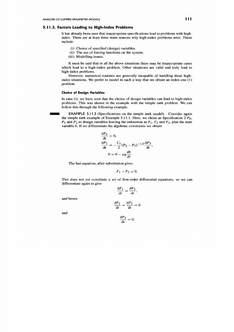
8/17/2019 Process Modelling and Model Analysis-Hangos-Cameron
http://slidepdf.com/reader/full/process-modelling-and-model-analysis-hangos-cameron 128/560
ANALYSIS OF LUMPED PARAMETER MODELS I I I
5.11.3. Factors Leading to High-Index Problems
It has already been seen that inappropriate specifications lead to problems w ith high-
index. There are at least three main reasons why high-index problems arise. These
include:
(i) Choice of specified (design) variables,
(ii) The use of forcing functions on the system,
(iii) Modelling issues.
It must be said that in all the above situations there may be inappropriate cases
which lead to a high-index problem. Other situations are valid and truly lead to
high-index p roblems.
However, numerical routines are generally incapable of handling these high-
index situations. We prefer to model in such a way that we obtain an index-one (1)
problem.
Choice of Design Variables
In case (i), we have seen that the choice of design variables can lead to high-index
problems. This was shown in the example with the simple tank problem. We can
follow this through the following example.
• • • EXAMPLE
5.11.3
(Specifications on the simple tank model). Consider again
the simple tank example of Example 5.11.1. Here, we chose as Specification 2 PQ,
P\ and P2 as design variables leaving the unknowns as F\, F2 and F 3, plus the state
variable
/?.
If we differentiate the algebraic constraints w e obtain
dFi
"dT
= 0,
The last equation, after substitution gives
Fi - F2 = 0.
This does not yet constitute a set of first-order differential equations, so we can
differentiate again to give
dFi dF2
dr ~ dr '
and hence
dFi ^ dF2 ^ ^
dt ~ dr
and
dF3
d , " •

8/17/2019 Process Modelling and Model Analysis-Hangos-Cameron
http://slidepdf.com/reader/full/process-modelling-and-model-analysis-hangos-cameron 129/560
I 12 CHAPTER
5
DY NA MIC MODEL S—LUMP ED PARAMETER SYSTEMS
This is an index-2 problem . A cursory observation on the system will easily show
that the suggested specification leads to
a
steady-state situation which is reflected in
• • • the above analysis.
Use of Forcing Functions and Modelling Issues
These reasons can also lead to high-index prob lems. In the case of forcing functions
we can add extra equations to the DAE set which are expressed only in terms
of
the
existing variables.
Inconsistent equations du e to poor modelling p ractice can also lead to high-index
problems.
Mo re details on these issues can be found in Gani and Cameron [38] and Hangos
and Cameron [39].
5.11.4. Consistent Initial Conditions
Accompanying the issue of high-index is that of consistent initial conditions. With a
pure O DE system w e are required to set the initial conditions of the states (differential
variables) x , in order to solve the problem. That is,
x=f(x,t\ (5.96)
weneedjc(O) =xo.
We can, in this case, set jc(0) to arbitrary values.
However,
it can be the
case w ith DAE systems that
the
additional algebraic
equations impose added constraints such that
it is
not possible
to
arbitrarily set the
values of jc(0). This can be seen from the previous examples.
I^^H EXAMPLE
5.11.4
(Consistent initial conditions
of
a linear DAE system).
The
previous Example
5.11.2
with the algebraic constraint
0 = jci +
2JC2
(5.97)
led to the relation
0 = i i+ 2j C 2. (5.98)
So,
the initial conditions of the states are related and
x i (0 ) = -2 x 2 (0 ) , ( 5.9 9)
JCI(0) = - 2 J C 2 ( 0 ) . (5.100)
I I I This means that only one state can be specified in an arbitrary way.
Wt^M EXAMPLE
5.11.5
(Consistent initial conditions for a tank problem). In the
simple tank model (see in Example 5.11.1) we gave a specification (Specification
2) [/atm*
P\,
^ 2 ] ^ which led to an index-2 problem.
The im plication of the analysis is that there is no possibility of selecting h(0) to
be an arbitrary value, since
hiO) = 0.
(5.101)
8/17/2019 Process Modelling and Model Analysis-Hangos-Cameron
http://slidepdf.com/reader/full/process-modelling-and-model-analysis-hangos-cameron 130/560
ANALYSIS OF LUMPED PARAMETER MODELS I I 3
One other major issue is to do with the initialization of the
algebraic
variables z.
It is often the case that the numerical routine will fail at the starting point if the values
;c(0) are not sufficiently close to the steady-state values c orrespon ding to jc(0).
Thus, we have a consistent set
x(0)
and often need to ensure that the value of the
algebraic residuals given by
8(x{0),zj) (5.102)
is close to zero by choosing the initial values z(0) to make
IU(jc(0),z(0),OII<^.
• • • In some cases , it can mean solving an algebraic set to get an initial steady state.
The problem of specifying consistent initial conditions for DAEs was first
addressed by Pantelides [40] and has been the subject of various approaches since
then [4 1]- [43 ]. It can often be a frustrating issue and is very dependen t on the problem
structure.
5.11.5. Model Stability and Stiffness (Ill-Conditioning)
One of the major problems which arises in process modelling is the issue of model
stiffness or ill-conditioning. This characteristic of the model in turn puts significant
demands on the numerical techniques which can be used to solve such problems.
The characteristic of ill-conditioning can be seen in a number of ways:
(i) the "time cons tants" of the process,
(ii) the eigenvalues of the model equations .
Many ph ysical system s display behaviour which is characterized by a wide range
of time constants in the system. The "time constant" reflects in some way just how
slowly or quickly a particular component or phenomenon reacts to a disturbance in
the system or to the action attributed to it. For example, in a reaction system where
we have a CSTR, there may be reactions which occur very quickly, whilst others are
very slow.
The fast reactions
are associated with
small time constants
whilst the
slow
reactions
are related to the
large time constants
of the system. These time constants
are related to the eigenvalues of the system equations as
r / a - - , (5.103)
where T/ is the time constant and A,/ is the real part of the system eigenvalue.
Hence, components (small time constants) correspond to large eigenvalues and
vice versa. Where we have a system with a mixture of widely varying time constants
we expect to see ill-conditioned behaviour.
To
appreciate the reason for
the
difficulties encoun tered in some problem s we turn
to investigate the
underlying stability
of the mathem atical mo del. It tells us something
about how errors are propagated as we solve the problem.
8/17/2019 Process Modelling and Model Analysis-Hangos-Cameron
http://slidepdf.com/reader/full/process-modelling-and-model-analysis-hangos-cameron 131/560
I 14
CHAPTER 5 DYNAMIC MODELS—LUMPED PARAMETER SYSTEMS
5.12. STABILITY OF THE MATHEMATICAL PROBLEM
Key Concept
The propagation of errors is not only depend ent
on
the type of method used but is influ
enced dramatically by the behaviour of the problem, notably by the integral curves,
which represent the family of solutions to the problem. This is clearly dependent on
the individual problem.
Before looking at analysing the problem to appreciate various behaviours, we
consider a general linear problem which gives some insight into solving general
problems.
• • • EXAMPLE 5.12.1 (Stability of a simple linear ordinary differential system).
Before ad dressing the general nonlinear O DE system, let us look at a simple 2 variable
problem to illustrate some basic characteristics.
Consider the problem
^ = / = Ay + 0 , (5.104)
at
where j i (0 ) = 0; y2(0) = -2
Th e exact solution is given by
y^(t) = -1.499 e-^-^^ 4- 0. 49 9e "^ ^^ ^ + 1, (5.106)
y2(t) = -2. 99 9e -^- ^^ - 0.0025e-2^^^^^ + 1. (5.107)
Note that the first terms in each equation represent the slow transients in the solution
whilst the second terms are the fast transients (see the exponential term s). Finally, the
constant terms represent the steady state values. The slow transients determine just
how long it takes to reach steady state. We can note that the fast transient is over at
t = 0 .002 w hilst the slow transient is over at r = 10.
If we solved this with a classical Runge-Kutta method, we would need about
7000 steps to reach steady state. Even though the fast transient has died out quickly,
the eigenvalue associated with this component still controls the steplength of the
I I I method when the method has a finite limit on the solution errors.
We need to analyse the general problem to appreciate the implications.
5.12.1 . The Mathematical Problem
Now let us consider the general nonlinear set of ODEs given by
y=fit,y) y(a)=yo, te{a,b). (5.108)
The behaviour of the solution to the problem near a particular solution g(t) can be
qualitatively assessed by the linearized variational equations given by:
y = J (^
g(t))[y - g{t)] +f(t, g(t)),
(5.109)
where J =
Sfj/dyj
is evaluated at
{t ,
g{t)).
8/17/2019 Process Modelling and Model Analysis-Hangos-Cameron
http://slidepdf.com/reader/full/process-modelling-and-model-analysis-hangos-cameron 132/560
STABILITY OF THE MATHEMATICAL PROBLEM
I I 5
Since the
local
behaviour is being considered, the Jacobian could be replaced
by a constant matrix A provided the variation of J in an interval of t is small. This
represents a "snap sho t" of the problem.
Assu ming that the matrix A has distinct eigenvalues A/, / = 1, 2 , . . . , n and that
the eigenvectors are v/, / = 1, 2 , . . . , n the general solution of the variational equation
has the form
n
yit) = J2^i^^^'^i-^Sit)' (5.110)
i=\
It is the value of e^' w hich charac terizes the local response to perturbations about the
particular solution
g(t).
There are three important cases related to the eigenvalues, which illustrate the
three major classes of problems to be encountered.
Unstable Case
Here, some A/ are positive and large, hence the solution curves fan out. A very
difficult prob lem for any ODE m ethod. This is
inherent instability
in the m athematical
problem.
This phenomenon can be seen in the following example.
• • • EXAMPLE
5.12.2
(Unstable ordinary differential equation ). Con sider the solu
tion of the following ordinary differential equation (ODE-IVP):
/ = y-t, yiO) = L
(5.111)
This has the general solution
y = Ae ' + r + I , (5.112)
so that the dominant term Ae^ is eliminated by applying the initial cond itions to give
A = 0.
Hence, the dominant term is
theoretically absent
but when small errors are
• • • introduced in the numerical solution this term can grow faster than the true solution.
This is an inherently u nstable problem with a positive eigenvalue of A. = 1. It is
clear that as this problem is integrated n umerically, the solution will continue to grow
without boun d as tim e heads for infinity.
Some process engineering problems have this type of characteristic. Some
catalytic reactor problems can exhibit thermal runaway which leads to an unsta
ble situation when a critical temperature in the reactor is reached. Certain processes
which have a control system installed can also exhibit instability d ue to unsatisfactory
controller tuning or design.
Stable Case
Here the X/ have negative real parts and are small in magn itude and hence the solution
curves are roughly parallel to
g(t).
These are reasonably easy problems to solve,
using conventional explicit techniques like Euler or Runge-Kutta methods. Stable
problems are also common in process engineering.
8/17/2019 Process Modelling and Model Analysis-Hangos-Cameron
http://slidepdf.com/reader/full/process-modelling-and-model-analysis-hangos-cameron 133/560
I I 6
CHAPTER 5 DYN AMI C MODELS—LUMPED PARAMETER SYSTEMS
Ultra Stable Case
Here, some
A,/
are large and negative (there are others that are small and negative) and
the solution curves quickly converge to g(t). This behaviour is good for propagation
of error in the ODE but not for a numerical method. This class of problems is called
''stijf'\ When inappropriate numerical methods such as Euler's method is applied to
an ultra stable problem then there is bound to be difficulties.
These problems occ ur frequently in process dyn amics, reaction kinetics, control
system responses, heat transfer, etc.
Other terms for "stiffness" are "ill-conditioning", or "widely separated time
constants" or "system with a large Lipschitz constant".
It should be noted that stiffness is a property of the mathematical problem not
the numerical method.
The phenom enon of stiffness is illustrated by the following exam ple.
• • • EXAMPLE
5.12.3
(An example of a stiff ordinary differential eq uatio n). Con
sider the problem given by
%=^y.
j (0) = [2 , l f , r e
[0 ,10] ,
(5.113)
where the matrix A is given by
.
/ - 50 0 . 5 499 .5 \
^.^^.^
^ = = ( , 4 9 9 .5 - 5 0 0 .5 j - ^^'^^^^
The exact solution to this linear ODE is
yi = 1.5e- + 0.5e-^^^^^ (5.115)
^2 =
1.5e-^-0.5e-l^^^^
(5.116)
Eigenvalues of the Jacobian of A are A, i =
— 1(XX); X2
= —1. Hen ce, the problem has
the initial transient followed by the integration of the slower transient as seen in the
analytic solutions. However, in the "stiff" region, which is close to when the steady
state is being approached, the fast componen t that has already decay ed to a very small
value still controls the steplength since
stability bound for method
' ' " '^ = R ea '> • ^^-^' ^
• • • In the case of Eule r's method , the stability bound is located at —2.
5.12.2. Comments
1.
It can be seen from the above example that the solution contains a very fast
component e~
^^^^
and a slow comp onent e~ ^ Obviously, the fast com ponent
quickly decays to zero and during this time, the numerical method will be
taking small steps to preserve accuracy while integrating this component.
Once this component has decayed, it could be thought that the steplength of
the numerical method could be increased solely on the basis of integrating the
slow component until steady state is reached. However, in many cases this
8/17/2019 Process Modelling and Model Analysis-Hangos-Cameron
http://slidepdf.com/reader/full/process-modelling-and-model-analysis-hangos-cameron 134/560
SUMMARY
I 17
is not
SO,
since the fast component can quickly increase without bound, thus
destroying the solution. It is important to minimize the steplength restriction
of the method by using an appropriate numerical scheme
so that only solution
accuracy determines the steplength. In general, we can state that:
• the largest negative eigenvalue controls integration steplength, while
• the smallest eigenvalue controls the integration time to the steady state.
2. It must also be emphasized that the "stiff-region" is where the particular
solution is dominating. That is, after the initial transient has decayed.
3. It is quite common in the literature to see reference made to the "stiffness
ratio" of a problem, this being an attempt to quantify the degree of stiffness.
It is generally defined as
max/ I Xi I
S{t)= , \ ' / ' (5.118)
mm / I ki I
This is
unsatisfactory
for several reasons, and should
no t
be used to
quantify the difficulty in solving a problem, since
• often some A,/ = 0 due to conservation law s;
• it is not generally true that
h~^ =
min/(Re(—A./)) as the definition
implies.
The fact that is of
greatest importance
is max
(— kih),
where
h
is the
stepsize, that accuracy would allow if stability was not a limitation. Hence,
as an alternative we co uld use the definition that
S(t) =
max (Re(-X //i)) (5.119)
noting that
the definition is dependent on the particular method being
used.
4. The example used to illustrate the problem of stiffness is linear. Most problem s
are in fact nonlinear and this means that the "stiff" region can change with
the independen t variable. A problem may be initially
"stiff"
and then become
"non-stiff or vice versa.
5. For the ultra-stable case application of an inappropriate m ethod for stiff equa
tions (i.e. Euler's m ethod) can produce a numerical solution which beco mes
unstable.
5.13. SUMMARY
This chapter has introduced the idea of lumped parameter balance volumes in order
to establish conservation equations for mass, energy or momentum. The particular
balances written will depend on the purpose of the modelling as well as the physics
and chemistry of the process system.
The idea of conservation balances was developed showing the general form of
each balance as well as the importance of individual terms within the balance equa
tions. In all cases, the conservation b alances w ere written using
extensive
variables. It
was shown that in som e circumstan ces it is necessary to have the balance equations in
intensive
variable form. However, the transformation to intensive variable form can
lead to more com plex relationships as well as com plications in the numerical solution
of such systems. These issues will be dealt with in Chapter 6.
8/17/2019 Process Modelling and Model Analysis-Hangos-Cameron
http://slidepdf.com/reader/full/process-modelling-and-model-analysis-hangos-cameron 135/560
I 18
CHAPTER 5 DYN AMIC MODELS—LUMPED PARAMETER SYSTEMS
5.14. REVIEW QUESTIONS
Q5.1. Wh at are the general expressions for total mass and com ponent mass balances?
Describe the significance of each term. (Section 5.3)
Q5.2. Wh at is the general expression for the energy balance over a defined region?
Describe the various terms in the balance equation and the significance of each.
(Section 5.4)
Q5.3.
When is it likely that a mom entum balance would be used in mod elling a
process system? (Section 5.5)
Q5.4.
Wh at are dimens ionless variables? Why is the concept imp ortant?
(Section 5.8)
Q5.5. Wh at is the aim of normalizing conservation balance equations? (Section 5.8)
Q5.6.
Describe why conservation balances might need to be written using intensive
rather than extensive variables. (Section 5.7)
Q5.7. Wh at are the advantages and disadvantages of writing conservation balances
in intensive variable form? (Section 5.7)
Q5.8.
Describe the importance of DO F in mod elling practice. W hat are the key steps
in carrying out the analysis? (Section
5.11.1)
Q5.9.
Why is the index of a DAE system impo rtant and how can it be assessed?
What factors give rise to high-index problems? (Section
5.11.2)
Q5.10. What are consistent initial conditions as applied to DAE systems? Why are
they important? (Section
5.11.4)
Q5.11.
Describe w hat is meant by model stability and how is it assessed? W hat does
this tell you abo ut
the
underlying behaviour of the model of the system? (Section 5.12)
5.15. APPLICATION EXERCISES
A5.1. For the Exercise A2.1 in Chapter 2, develop the mass and energy balances for
the system after defining the balance volumes for mass and energy.
A5.2.
Consider the energy balance of Exam ple 5.6.1. Normalize this equation by a
suitable choice of normalizing variables.
A5.3.
For Exercise A2.2 in Chapter 2, define balance boundaries and then develop
the conservation balances for both mass and energy for those balance volumes.
A5.4. Take the problem in Exercise A3.1 of Chap ter 3, and consider the case where
the tank is now enclosed. D evelop both mass and energy balances for this new system.
Wh at has changed? Is it significant in terms of the dynam ics?
A5.5.
Develop
a
mathem atical model for
the
domes tic water heater shown in
Fig.
5.7.
Water flowrate is variable but the temperature needs to be controlled to a desired
setpoint. To do this, an electric immersion heating coil is adjusted by a temperature
control loop. Develop the model in a structured w ay following the model developm ent
framework:
(a) define the problem,
(b) identify all relevant controlling factors,

8/17/2019 Process Modelling and Model Analysis-Hangos-Cameron
http://slidepdf.com/reader/full/process-modelling-and-model-analysis-hangos-cameron 136/560
APPLICATION EXERCISES
cold water
119
Heater
0
©
^ hot water
- C ^ ] •
F I G U R E 5 . 7 Domestic hot-wate r heater.
(c) State the data you require and where you migh t access it,
(d) state all your modelling assum ptions and justify them,
(e) clearly indicate your balance boundaries,
(f) develop the mathematical mo del and clearly state the development steps,
(g) analyse the equations for degrees of freedom.
A5.6. Con sider the process of blending two streams of liquid in a tank where all
streams can vary in flowrate. The main stream (1) contains two co mpo nents (A and
B)
whilst the second stream (2) contains only com ponent B. Both streams are at different
temperatures. The goal is to add stream 2 in order to maintain a fixed concentration
of B in the outlet from the blending tank. The outlet from the tank is pumped under
level control. Figure 5.8 shows the process.
stream 2
o^
Er
F I G U R E 5 . 8 Liquid blending system.

8/17/2019 Process Modelling and Model Analysis-Hangos-Cameron
http://slidepdf.com/reader/full/process-modelling-and-model-analysis-hangos-cameron 137/560
120
CHAPTER 5 DY NA MIC MODELS —LUM PED PARAMETER SYSTEMS
Develop the model in a structured way following the model development
framework and the key steps given in Exercise A5.5
A5.7. An ice cube is placed into a cylindrical plastic container of water which is
initially at room temperature and begins to dissolve. Consider the case where the
tumbler con tents are stirred to help dissolve the ice cube. Develop a model, using the
mod elling framework, to predict the dynam ics of the system over the short term and
long term.
One of the key parameters of the system will be the overall heat transfer coefficient
of the melting ice cube . Make an estimate or predict its value.
Use typical values for the system of 25°C ambient temperature for the water,
container liquid volume of 250 ml and a rectangular shaped ice cube of approxim ately
25 cm^. Typical aspect ratio of the ice-cube is 1:1.25:2.5. It will be necessary to state
clearly the value and accuracy of all parameters used in the mod el.
A5.8. A CSTR is a comm on piece of processing equipm ent. In this application,
consider the mod elling of a CSTR for startup and control purpo ses. In this case, there
is a cascade of three jacketted CSTRs in series with cooling provided in either a
cocurrent or countercurrent direction. The cascade is shown in Fig. 5.9 and indicates
a countercurrent flow situation.
^ C ' ^ C
F I G U R E 5 ,9 Cascade of continuous st irred tank reactors.
coolant
Because of the physico-chem ical nature of this system, m ultiple steady states can
occur due to the balance between cooling and heating in each reactor. This directly
affects the performance of the reactors. In one case, low temperatures in both reactor
and cooling systems leads to low conversions of around 20%. In contrast, the high-
temperature scenario leads to conversions around
99%.
Other intermediate states are
also possible in this system.
Data on the problem are as follows:
• The reaction is first-order exotherm ic,
A -> B,
with
r = kCA,
and
k =
kQQ-E/iRT)i^^ ^2000s-K
• Heat transfer area per reactor, A H = 0.09 m^.
• Reactor volume, V/ = 0.8 m- , cooling jacket volume, VQ = 0.1 m^.
• Heat capacity of mixture , Cp =
0.565
kJ/kgK , heat capacity of coolant, Cpc =
4.1868kJ/kgK.
• Density of mixture, p = 850 kg/m ^, density of coolant, pc = 1000 kg/m^
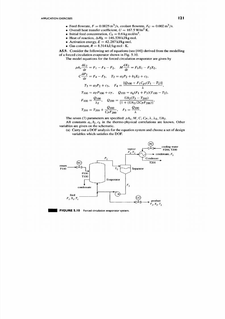
8/17/2019 Process Modelling and Model Analysis-Hangos-Cameron
http://slidepdf.com/reader/full/process-modelling-and-model-analysis-hangos-cameron 138/560
APPLICATION EXERCISES
121
Feed flowrate,
F
= 0.0025 m^/s, coolant flowrate,
F Q -
0.002 m ^/s.
Overall heat transfer coefficient, U = 167.5 W/m^ K.
Initial feed concentration, CQ = 0.6kgmol/m^.
Heat of reaction, A / / R = 146,538 kJ/kgm ol.
Activation energy,
E =
42,28 7 kJ/kg mol.
Gas constant, R = 8.314 kJ/kg mol • K.
Con sider the following set of equations (see [44]) derived from the mod elling
of a forced circulation evaporator shown in Fig. 5.10.
The model equations for the forced circulation evaporator are given by
A5.9.
pA,
dL2
dt
F\ — F4 —
F2,
M ^ = F iX i ^ F 2X 2,
at
T2 = a2P2 + h^ 2 + C2,
[Q\00-^F\CpiiTi
T2)]
T3=a3P2 +
C3, F4
A
7^100 = CITPIOO + CT, GlOO = ciqiFi + F^^TioQ - 7^2),
GlOO ^ ^^2( 7^3 - ^200)
^100 =
^201 =
7200
+
G2OO
=
6200
CpF200'
[ l + ( [ M 2 / 2 C p F 2 0 0 ) ] '
r Q200
The seven (7) parameters are specified: pAs, M, C, Cp, X, As, UA2.
All constants
ai.bj^Ck
in the thermo-physical correlations are known. Other
variables are given on the schematic.
(a) Carry out a DO F analysis for the equation system and ch oose a set of design
variables which satisfies the DOF.
steam
FlOO
cooling water
vapour j; u-^-r F200, T200
> t^ \ /^ • condensate, F^
Condenser
LC)
» n > ^ > product
FIGURE
5.10
Forced circulation evaporator
system.

8/17/2019 Process Modelling and Model Analysis-Hangos-Cameron
http://slidepdf.com/reader/full/process-modelling-and-model-analysis-hangos-cameron 139/560
I 22
CHAPTER 5 DYN AMIC MODELS—LUMPED PARAMETER SYSTEMS
(b) Check that the choice of design variables leads to an index-1 problem .
(c) Are there choices which lead to index-2 or higher systems? Explain the
significance of the specifications which lead to these situations.
A5.10.
Develop and analyse a dynam ic model for the behaviour of a pool of diethyl-
amine (DBA) (CH3CH2)2NH, which forms after a spill to ground. Assume that the
bounded area is
25
m^ and that the initial spill gives a pool depth of
100 mm.
A wind
of 3 m/s is blowing and the ambient temperature is 26°C. The pool is formed over
a concrete pad whose temperature is constant at 40°C. The incoming solar radiation
level is
950
W m - 2 .

8/17/2019 Process Modelling and Model Analysis-Hangos-Cameron
http://slidepdf.com/reader/full/process-modelling-and-model-analysis-hangos-cameron 140/560
SOLUTION STRATEGIES
FOR
LUMPED PARAMETER MODELS
This chapter considers the numerical solution of lumped parameter models resulting
from the application of either steady-state or dynamic conservation balances on a
process system. In particular, we consider the numerical solution of both nonlinear
algebraic equations (NLAEs) and ordinary differential equations-initial value prob
lems (ODE-IVPs). In the context of process engineering, dynamic modelling often
leads to mixed system s of OD Es and NLA Es. These are termed differential-algebraic
equations or DAEs. Approaches to the numerical solution of such systems are also
discussed. In some cases, lumped parameter models lead to ordinary differential
equations-boundary value problems (ODE-BVPs). The solution of these types of
problems is discussed in Chapter 8.
This chapter commences with some typical examples of the types of problems
often requiring numerical solution. It is followed by an introduction to some basic
definitions of important terms frequently used in the context of numerical solu
tion of ODEs. Consideration is then given to stability analysis of the methods and
how this concept interacts with the stability of the actual problem. Several practical
implications of these issues are discussed.
In presenting the numerical solution approaches, two major classes of numerical
methods are introduced which have widespread application and availability. These
are classified as linear multi-step methods (LMMs) and single-step methods. Several
examples of both methods are introduced and their characteristics are discussed.
To conclude, we discuss the numerical solution of DAE systems using a variety
of approaches and discuss the advantages and disadvantages of the techniques.
123
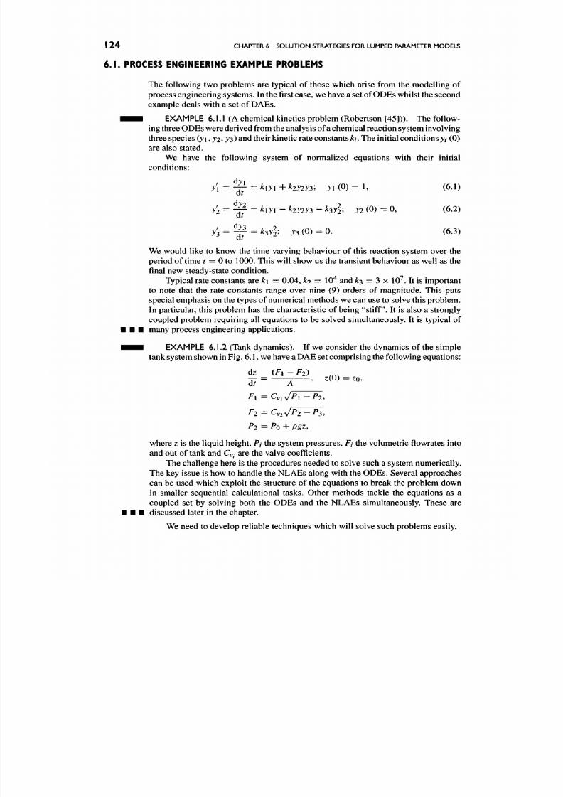
8/17/2019 Process Modelling and Model Analysis-Hangos-Cameron
http://slidepdf.com/reader/full/process-modelling-and-model-analysis-hangos-cameron 141/560
I 24 CHAPTER 6 SOLUTION STRATEGIES FOR LUMPED PARAMETER MODELS
6.1. PROCESS ENGINEERING EXAMPLE PROBLEMS
The following two problems are typical of those which arise from the modelling of
process engineering systems. In the first case , we have a set of OD Es whilst the second
example deals with a set of DAEs.
W^m EXAMPLE 6.1.1 (A chem ical kinetics problem (Robertson [45]) ). The follow
ing three ODE s were derived from the analysis of a chemical reaction system involving
three species (y i, >2» J3) and their kinetic rate constants kj. The initial conditions yi (0)
are also stated.
We have the following system of normalized equations with their initial
conditions:
y\
= ^ =
^i>'i + ^2J2J3;
y\
(0) = 1, (6.1)
y2 = ^ = ^^y^ -
^2y2y3
- hyl; yi
(0) - o, (6.2)
J3 = ^ = ^3 25 y^ (0) = 0- (6.3)
We would like to know the time varying behaviour of this reaction system over the
period of time r = 0 to 10(X). T his will show us the transient behaviour as well as the
final new steady-state co ndition.
Typical rate constants are
k\ =
0.04, k2
=
10" and ^3 = 3 x 10^. It is important
to note that the rate constants range over nine (9) orders of magnitude. This puts
special emphasis on the types of num erical methods we can use to solve this problem.
In particular, this problem has the characteristic of being
"stiff.
It is also a strongly
coupled problem requiring all equations to be solved simultaneously. It is typical of
• • • many process engineering applications.
• • • EXAMPLE 6.1.2 (Tank dynamics). If we consider the dynamics of the simple
tank system shown in Fig. 6.1, we have a DAE set comp rising the following equa tions:
dz ( F 1 - F 2 ) ._.
— = , z(0) = zo.
at A
Fl=Cy,y/Pl-P2,
Fl = Cy,^P2-P3.
where z is the liquid height, P/ the system pressures, F/ the volumetric flow rates into
and out of tank and Cv^ are the valve coefficients.
The challenge here is the procedu res needed to solve such a system numerically.
The key issue is how to handle the NLA Es along w ith the ODE s. Several approaches
can be used which exploit the structure of the equations to break the problem down
in smaller sequential calculational tasks. Other methods tackle the equations as a
coupled set by solving both the ODEs and the NLAEs simultaneously. These are
discussed later in the chapter.
We need to develop reliable techniques which will solve such problems easily.

8/17/2019 Process Modelling and Model Analysis-Hangos-Cameron
http://slidepdf.com/reader/full/process-modelling-and-model-analysis-hangos-cameron 142/560
ORDINARY DIFFERENTIAL EQUATIONS
125
^ 1
iX\-
m FIGURE 6.1 Simple tank dynamics.
6.2. ORDINARY DIFFERENTIAL EQUATIONS
The basic problem we wish to solve is a set of ODEs given in general terms by
y=f(yj)
y(a)=yo. (6.4)
where t e (a , b ) and j e /?'^ (y is a n-dimension al v ector of real num bers). T his
represents a system of first-order ODEs with initial values.
This is a vector of equations in the variables y . Note that it is necessary to state
the initial values of all the y variables at r = a. The solution is required over the time
interval
(a,b).
6.2 .1 .
Higher Order Equations
Sometimes, after modelling a process system, we have equations containing higher
order derivatives. For the case of higher order systems, we can reduce these to first-
order equations, which are then easily solved by standard techniques.
If we consider the following higher order ODE
where
y^"^
represents the nth derivative of
j .
By making a series of substitutions for the derivative terms of the form:
3 , , = / - ) =
d t ' - " j
we can transform the higher order equation into a set of n first-order OD Es.
Normally the initial conditions for the higher order equation are given as
Gi ( > '' " -" ( 0 ), 3 ; f" - 2 » (0 ) ,. . . . y f ' k O ) , ^ ^ )
=
0,
and using the same substitutions we can reduce these conditions to
j , ( 0 ) = / - > > ( 0 ) .
(6.5)
(6.6)
(6.7)
(6.8)

8/17/2019 Process Modelling and Model Analysis-Hangos-Cameron
http://slidepdf.com/reader/full/process-modelling-and-model-analysis-hangos-cameron 143/560
I 26 CHAPTER 6 SOLUTIO N STRATEGIES FOR LUMPED PARAMETER MODELS
• 1 ^
EXAMPLE 6.2.1 (A second-order system ). Consider the higher (2nd) order
equation
^+f(y) = 0
w i t h ^ ( 0 ) = c i;
y{0) =
C2.
(6.9)
To transform to a set of first-order OD Es, w e let
y\=y. (6.10)
j 2 = y = ^ , (6.11)
hence, we get two ODEs with their respective initial conditions:
^ + / ( J ) = 0; J 2(0 ) = c , , (6.12)
at
~ ^ = J 2 ;
y\(0) = c2.
(6.13)
6.2.2. Conversion to Autonomous Form
This removes the explicit presence of the independent variable
t
from the right-hand
side functions. T his we call the "autono mo us" form of the problem. We define a new
variable yn-\-\ so that we have
y = ^
=f(y\
(6.14)
y[,^^ = l and y„ +i(0 ) = 0. (6.15)
In most modern numerical methods, the value of the independent variable can be
retained in the right-hand side functions.
6.3. BASIC CONCEPTS IN NUMERICAL METHODS
Key concept
A discretization or numerical solution of
an
initial value problem is a sequence of
discrete values
[yn}n£Ni
where N is the set of integers, computed via a method Fn
which solves at each step the algebraic equations given by
Fnyn^O, neN. (6.16)
Note that Fn represents some general form of algebraic equation which is solved for
yn at each step.
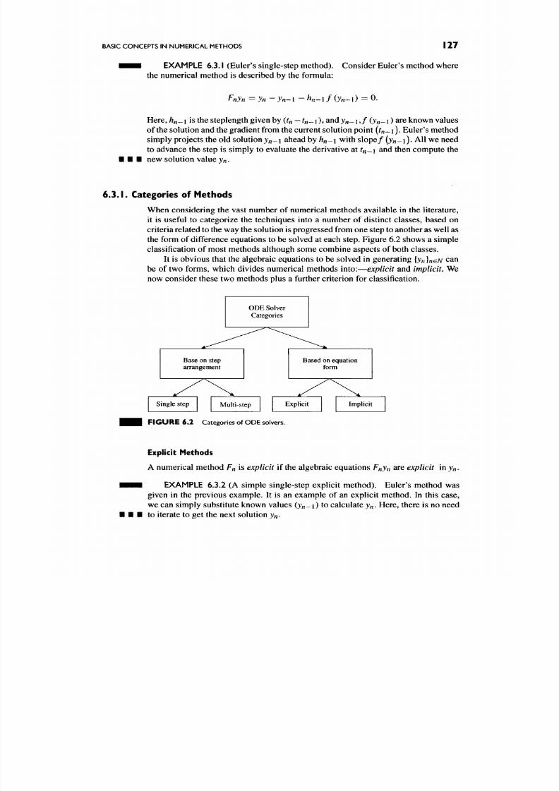
8/17/2019 Process Modelling and Model Analysis-Hangos-Cameron
http://slidepdf.com/reader/full/process-modelling-and-model-analysis-hangos-cameron 144/560
BASIC CONCEPTS IN NUMERICAL METHODS
127
EXAMPLE 6.3.1 (Euler's single-step method),
the numerical method is described by the formula:
Consider Euler's method w here
Fnyn =yn-
J / i - l -
K - X f
( j n - l ) == 0 .
• • •
Here , /z„_i is the steplength given by {tn — tn-\), an d y „_ i , / (y^_i) are known values
of the solution and the gradient from the current solution point (tn-\). Euler's method
simply projects the old solution j ^ _ i ahead by hn-\ with slo pe / ( jn -l) - All we need
to advance the step is simply to evaluate the derivative at r„_i and then comp ute the
new solution value yn.
6.3.1.
Categories of Methods
When considering the vast number of numerical methods available in the literature,
it is useful to categorize the techniques into a number of distinct classes, based on
criteria related to the way the solution is progressed from one step to another as well as
the form of difference equations to be solved at each step. Figure 6.2 shows a simp le
classification of most methods although some combine aspects of both classes.
It is obvious that the algebraic equations to be solved in generating
{yn}n£N
can
be of two forms, which divides numerical methods into:—
explicit
and
implicit.
We
now consider these two methods plus a further criterion for classification.
ODE Solver
Categories
Base on step
arrangement
Based on equation
form
Single step Multi-step Explicit Implicit
F I G U R E 6 .2 Categories of ODE solvers.
Explicit Methods
A numerical method
Fn
is explicit if the algebraic equations
Fnyn
are explicit in j ^ .
• EXAMPLE 6.3.2 (A simple single-step explicit meth od). Eu ler's method was
given in the previous example. It is an example of an explicit method. In this case,
we can simply substitute known values (y ^- l) to calculate
yn.
Here, there is no need
• to iterate to get the next solution j„ .

8/17/2019 Process Modelling and Model Analysis-Hangos-Cameron
http://slidepdf.com/reader/full/process-modelling-and-model-analysis-hangos-cameron 145/560
128 CHAPTER 6 SOLUTION STRATEGIES FOR LUMPED PARAMETER MODELS
Implicit Methods
A numerical method Fn is implicit if the algebraic equations Fnyn are implicit in yn.
In this case, we normally need to iterate the equations to get the solution for yn.
• • • EXAMPLE 6.3.3 (A simple single-step implicit method). Consider the Back
ward Euler method, which is an implicit version of the standard Euler method:
Pnyn =yn- j« - i - K-\f(yn) = 0.
Note that in this case the gr ad ien t/(y ,i) is being evaluated
at the e nd of the current
step, at time tn. Since we do not know y^ which is the solution at the end of the current
step, we have to guess it and iterate until we converge to the solution. Clearly, there is
significantly more w ork per step in this implicit method than in the equivalent exp licit
method. In the case of multiple equations, we need to solve a set of NLAEs for each
output p oint. It will be evident that there are characteristics of this m ethod that justify
• • • its use even though it is expensive computationally.
The discretization methods besides being either "explicit" or "implicit" can
also be classified as either "single step" or "multi-step" methods, depending on the
amount of information used in computing the next step. Thus we have the following
two methods.
Single-Step Methods
A numerical method is a
single-step
method, if it
only uses inform ation from the last
solution point or w ithin the current step to compute the new output value. Single-step
methods have been the most well known of all numerical integration routines and
date back many centuries.
• • • EXAMPLE 6.3.4 (Rung e-Kutta or Euler one-step methods). Euler's method or
the Runge-Kutta methods are regarded as single step methods because they only use
information at t^ -
\
to get to
tn-
They use information from the last computed solution
point y„_l or within the current step (r„_i to r„) to generate the new solution value
at tn. They do not use past points of the solution from r„_2, ^/i-3, . •., tn-k-
We can consider a Runge-Kutta method to see this characteristic, where the
solution for
yn
is given by
yn = yn-\ +hY^bifl tn-\ + Cfh, yn-\ + J^
^iJ^J
' ^^'^^^
In this method, there is no occurrence of past solution p oints, r„ _ 2 ,. .. .
Multi-step Methods
A numerical method is a multi-step method if it uses information from several past
solution points to calculate the new output point.
8/17/2019 Process Modelling and Model Analysis-Hangos-Cameron
http://slidepdf.com/reader/full/process-modelling-and-model-analysis-hangos-cameron 146/560
LOCAL TRUNCATION ERROR AND STABILITY
I 29
• • • EXAMPLE 6.3.5 (Linear multi-step methods). L MM s (of k steps) are typical
examples of these methods. They are expressed as
k k
j=0 j=0
where or/ and fi j are constants (either ao or Po are non-zero. Generally, a^ = 1).
Thus, for ^ = 2 we have
yn-\-2 =
- ( a o j n + a i ^ /i -f l ) +
hWofn
+ P\fn-^\ +
Plfn^l).
• • • which is a two-step method .
Remember that all the numerical methods involve computational errors since
they are metho ds wh ich attempt to approximate the solution over the range of interest.
Hence,
we
must app reciate what type of errors are involved in our numerical procedure
as well as the way these errors propagate as we attempt to solve the problem.
The key issue w hich w e have to face
is
choosing an appropriate numerical method
to solve our problem. T he method w e choose is strongly dictated by the characteristics
of the problem we are solving. Appreciating that aspect of the solution procedure is
vital. Hence, we consider the issues of truncation error and stability.
6.4. LOCAL TRUNCATION ERROR AND STABILITY
Here, w e want to develop the important relationships betw een stability of the solution
and the factors which affect it. Stability refers to how the errors committed by the
numerical approximation method propagate as the solution progresses. We want to
avoid solutions which "blow up" because of inappropriate methods or steplengths. In
order to see what is important in determining this, we consider a simple mathemat
ical problem of known solution and compare that with the solution generated by a
numerical method.
First, we establish some nomenclature by letting
y{tn) = the exact solution at tn , (6.18)
yn —
the numerical solution at
t n,
(6.19)
as a convention which will be used throughout this chapter.
We will consider a simple example p roblem by look ing at its
true solution
as well
as its numerical solution. C omparison of the two shows us how errors propagate.
6.4 .1 . Analytical Solution
Consider solving the linear system
/ = - A j , 0 < r < ff (6.20)
with initial conditions
j ( 0 ) = j o . ( 6 . 2 1 )

8/17/2019 Process Modelling and Model Analysis-Hangos-Cameron
http://slidepdf.com/reader/full/process-modelling-and-model-analysis-hangos-cameron 147/560
I 30 CHAPTER 6 SOLUTIO N STRATEGIES FOR LUMPED PARAMETER MODELS
The true solution from point
tn-\
to tn is easily calculated as
yitn) =
^-^^yitn-\), (6.22)
where
tn
= nh
and /i > 0. The exponential m atrix is readily c alculated.
Let us introduce the operator
S{z) =
e~^, we can rewrite Eq. (6.22) so that
y{tn) = S(\h)y{tn-i),
(6.23)
Hence, the analytical solution of the linear ODE from tn to tn-\ is obtained by
multiplying the last solution by the value
S(Ah),
which is the matrix exponential for
the set of equations. Now let us turn to the num erical solution.
6.4.2. Numerical Solution
For the numerical solution, let us use Euler's method as an example to see how the
solution is progressed from step to step.
The Euler method applied to the original problem in Eq. (6.20) gives
yn = Jn -1 + hfn-\ =yn-\- A/l J„_ l (6 .24)
with the initial co nditions
ym=yo.
(6.25)
Let the operator
K(z)
= (1 — z) be the "amplification" factor, then w e can write
the numerical solution as
yn = K{Ah)yn-i, (6.26)
Hence, the numerical solution progresses from step to step using the value K{kh)
which is dependent on the form of the method as well as the problem.
6.4.3. Global Error
We can now define the global error as the difference between the true solution and
the numerical solution. It is this value which we want to control during the solution
procedure:
Sn=y{tn)-yn^
(6.27)
Hence,
8n
-
S{kh)y(tn-\) - K{Ah)yn-U
(6.28)
8n = S(Ah)y(tn-i) - K(Ah)y{tn-i) - KiAh)yn-i + K{Ah)y(tn-i), (6.29)
8n = K Sn-X
+ (5 -
K )y{tn-l) .
(6.30)
8n^K 8n-\ + Ty{tn-\). (6.31)
Here, we let
T
— truncation operator.
Notice that the global error at
tn
cons ists of
two
parts. Th e first is the term
K8n-\
which represents that fraction of the previous global error which is carried forward
into the present step. Obviously, this should not be magnified and hence we require
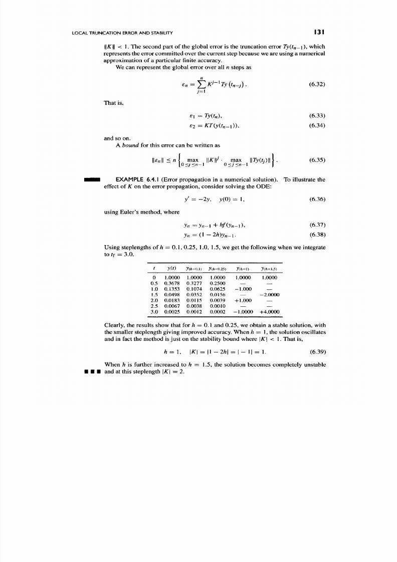
8/17/2019 Process Modelling and Model Analysis-Hangos-Cameron
http://slidepdf.com/reader/full/process-modelling-and-model-analysis-hangos-cameron 148/560
LOCAL TRUNCATION ERROR AND STABILITY I 3 I
\\K\\ <
1. The second part of the global error is the truncation error
Ty{tn-\),
which
represen ts the error com mitted over the current step because w e are using a num erical
approximation of a particular finite accuracy.
We can represent the global error over all n steps as
n
en = J2KJ-^Ty{tn-j), (6.32)
7 = 1
That is,
^1 = Tyitn), (6.33)
82 = KT(y(tn-i)),
(6.34)
and so on.
A
bound
for this error can be written as
\\sn\\ < n I m a x | |^ |K - m a x \\Ty(tj)\\\ . (6.35)
[0<j<n-\ 0<j<n-l ^
J
EXAMPLE 6.4.1 (Error propaga tion in a num erical solutio n). To illustrate the
effect of K on the error propagation, consider solving the ODE:
y = -2>; , j ( 0 ) = : l , (6.36)
using Euler's method, where
yn = Jn - l + hf(yn-\), (6.37)
3;;, = ( 1 - 2 % ^ _ 1 . (6.38)
Using steplengths of/i = 0.1, 0.25, 1.0, 1.5, we get the following when we integrate
toff = 3.0.
t
0
0.5
1.0
1.5
2.0
2.5
3.0
y(t)
1 0000
0 3678
0 1353
0 0498
0 0183
0 0067
0 0025
> (;i=o.i)
1 0000
0 3277
0 1074
0 0352
0 0115
0 0038
0 0012
y{h=0.25)
1 0000
0 2500
0 0625
0 0156
0 0039
0 0010
0 0002
y(h=i)
1 0000
—
-1.000
—
+ 1.000
—
-1.0000
> (/»=1.5)
1 0000
—
—
-2.0000
—
—
+4.0000
Clearly, the results show that for h = 0.1 and 0.25, we obtain a stable solution, with
the smaller steplength giving improved accuracy. When
h =
1, the solution osc illates
and in fact the method
is
jus t on the stability boun d w here lA'l < 1. That is,
h=l, \K\ = \l-2h\ = \-l\ = l,
(6.39)
When
h
is further increased
to h =
1.5, the solution becomes completely unstable
and at this steplength | ^ | = 2 .
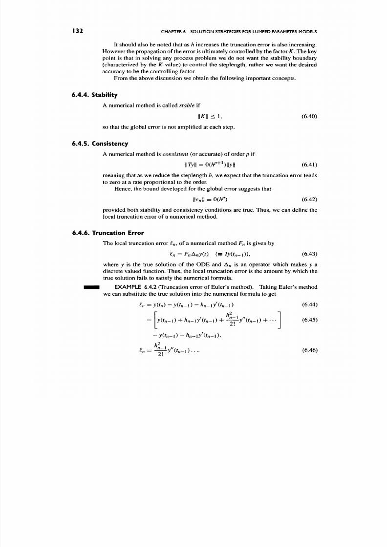
8/17/2019 Process Modelling and Model Analysis-Hangos-Cameron
http://slidepdf.com/reader/full/process-modelling-and-model-analysis-hangos-cameron 149/560
I 32 CHAPTER 6 SOLUTIO N STRATEGIES FOR LUMPED PARAMETER MODELS
It should also be noted that as
h
increases the truncation error is also increasing .
How ever the propagation of the error is ultimately controlled by the factor K. Th e key
point is that in solving any process problem we do not want the stability boundary
(characterized by the K value) to control the steplength, rather we want the desired
accuracy to be the controlling factor.
From the above discussion we obtain the following important concepts.
6.4.4. Stability
A numerical method is called
stable
if
ll^ll < 1, (6.40)
so that the global error is not amplified at each step.
6.4.5. Consistency
A numerical method is
consistent
(or accurate) of order/? if
\\Ty\\=0{hP^^)\\y\\ (6.41)
meaning that as we reduce the steplength h, we expect that the truncation error tends
to zero at a rate proportional to the order.
Hence, the bound developed for the global error suggests that
\\en\\==OihP)
(6.42)
provided both stability and consistency conditions are true. Thus, we can define the
local truncation error of a numerical method.
6.4.6. Truncation Error
The local truncation error €„, of a numerical method Fn is given by
in = FnAny(t) {^Ty(tn-i)). (6.43)
where
y
is the true solution of the ODE and A,i is an operator which makes
y
a
discrete valued function. Thu s, the local truncation error is the amount by which the
true solution fails to satisfy the numerical formula.
• • • EXAMPLE 6.4.2 (Truncation error of Eu ler's metho d). Taking Eule r's method
we can substitute the true solution into the numerical formula to get
^n = y(tn) - y(tn-\) - hn-\y\tn-\) (6.44)
(6.45)
{tn-i) + hn-iy\tn-l) + -^/{tn-l) +
-y(tn-l)-hn-iy\tn-\) .
^n
= -^y'{tn-l) . . . ,
(6.46)

8/17/2019 Process Modelling and Model Analysis-Hangos-Cameron
http://slidepdf.com/reader/full/process-modelling-and-model-analysis-hangos-cameron 150/560
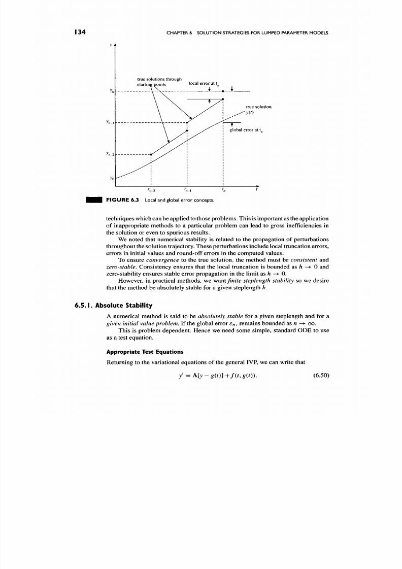
8/17/2019 Process Modelling and Model Analysis-Hangos-Cameron
http://slidepdf.com/reader/full/process-modelling-and-model-analysis-hangos-cameron 151/560
134
CHAPTER 6 SOLUTION STRATEGIES FOR LUMPED PARAMETER MODELS
true solutions through
starting points local error at t,,
* . ^ L
true solution
yit)
F I G U R E 6 . 3 Local and global er ror concepts.
techniques w hich can be applied
to
those problems. This
is
important
as
the application
of inappropriate methods to a particular problem can lead to gross inefficiencies in
the solution or even to spurious results.
We noted that numerical stability is related to the propagation of perturbations
throughout the solution trajectory. These perturbations include local truncation errors,
errors in initial values and round-off errors in the computed values.
To ensure convergence to the true solution, the method must be consistent and
zero-stable.
Consistency ensures that the local truncation is bounded SLS
h -^ 0
and
zero-stability ensures stable error propagation in the limit as /t - ^ 0.
However, in practical methods, we
wsint
finite stepleng th stability so we desire
that the method be absolutely stable for a given steplength
h.
6.5.1. Absolute Stability
A numerical method is said to be absolutely stable for a given steplength and for a
given initial value problem,
if the global error S n, remains bounded as n ^ - oo.
This is problem dependent. H ence we need some simple, standard OD E to use
as a test equation.
Appropriate Test Equations
Returning to the variational equations of the general IVP, we can write that
y = A [ j - g ( r ) ] - ^ / ( r , g ( 0 ) . (6.50)
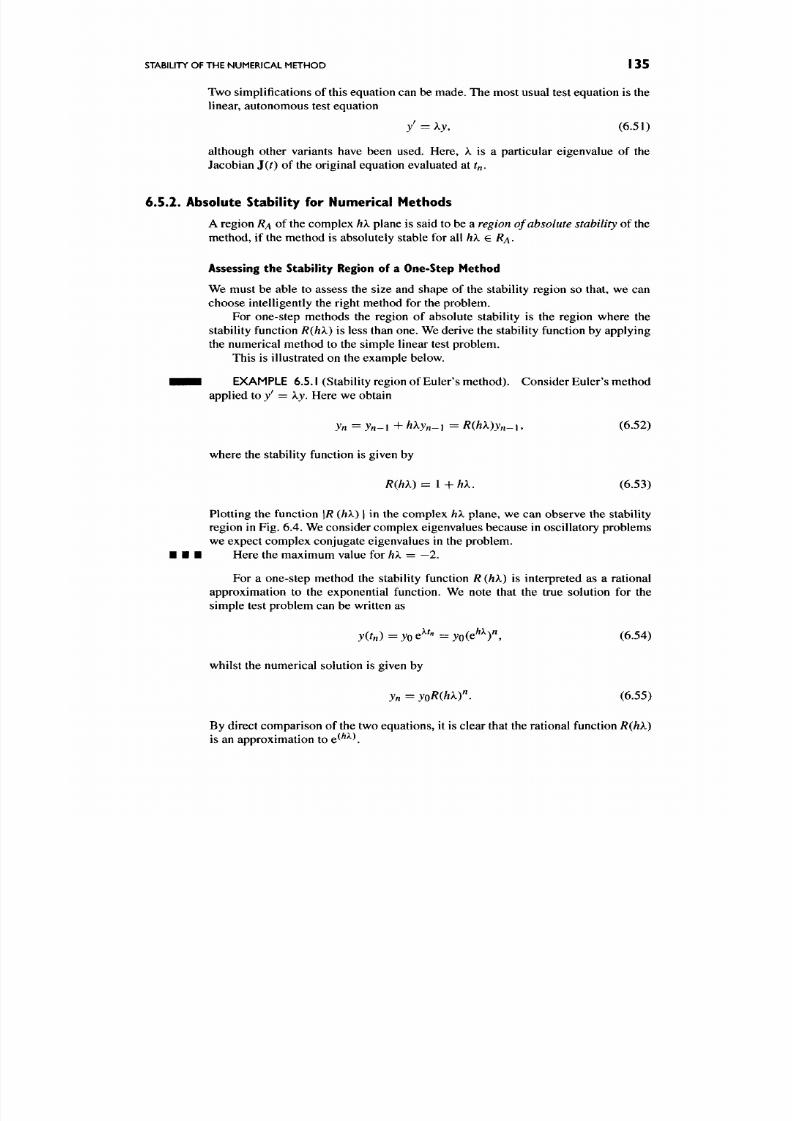
8/17/2019 Process Modelling and Model Analysis-Hangos-Cameron
http://slidepdf.com/reader/full/process-modelling-and-model-analysis-hangos-cameron 152/560
STABILITY OF THE NUMERICAL METHOD
I 35
Two simplifications of this equation can be m ade. The mo st usual test equation is the
linear, autonomous test equation
y = ^y.
(6.51)
although o ther variants have been used. Here, X is a particular eigenvalue of the
Jacobian J(0 of the original equation evaluated at r„.
6.5.2. Absolute Stability for Numerical Methods
A region RA of the complex hX plane is said to be a region
of absolute stability
of the
method, if the method is absolutely stable for all
hX e RA-
Assessing the Stability Region of a One-Step Method
We must be able to assess the size and shape of the stability region so that, we can
choose intelligently the right method for the problem.
For one-step methods the region of absolute stability is the region where the
stability function R(hX) is less than one. We derive the stability function by ap plying
the numerical method to the simple linear test problem.
This is illustrated on the example below.
• • • EXAMPLE 6.5.1 (Stability region of Euler's method). Consider Euler's method
applied to y' = ky. Here we obtain
yn =yn-\+ hXyn-
\
= R{hX)yn-
1, (6.52)
whe re the stability function is given by
R{hk) = \-^hX, (6.53)
Plotting the function \R (hX) \ in the complex hX plane, we can observe the stability
region in Fig. 6.4. We consider complex eigenvalues because in oscillatory problems
we expect complex conjugate eigenvalues in the problem.
• • • Here the maximum value for hX = —2.
For a one-step method the stability function
R (hX)
is interpreted as a rational
approximation to the exponential function. We note that the true solution for the
simple test problem can be written as
y(tn)=yo^^' =yo(^^^r, (6.54)
whilst the numerical solution is given by
yn=yoR(hX)\ (6.55)
By direct co mparison of the two equation s, it is clear that the rational function R(hX)
is an approximation to e^'^^^
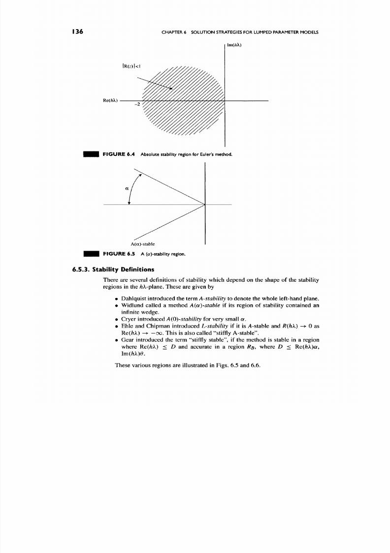
8/17/2019 Process Modelling and Model Analysis-Hangos-Cameron
http://slidepdf.com/reader/full/process-modelling-and-model-analysis-hangos-cameron 153/560
136 CHAPTER 6 SOLUTION STRATEGIES FOR LUMPED PARAMETER MODELS
Re(hX)
F I G U R E 6 . 4 Absolute stability region for Euler's method.
A(a)-stable
F I G U R E 6 . 5 A (a)-stability region.
6.5.3. Stability Definitions
There are several definitions of stability which depend on the shape of the stability
regions in the /iA,-plane. These are given by
• Dahlquist introduced the term
A-stability
to denote the whole left-hand plane.
• Widlund called a method A(a)-stable if its region of stability contained an
infinite wedge.
• Cryer introduced A(0)-stability for very small a.
• Ehle and Chipm an introduced
L-stability
if it is A-stable and
R{hk)
-> 0 as
Re(/?A) -> - 0 0 . This is also called "stiffly A-stab le".
• Gear introduced the term "stiffly stab le", if the method is stable in a region
where Re(AA.) < D and accurate in a region RB, where D < Re(hX)a,
lm{hX)0.
These various regions are illustrated in Figs . 6.5 and 6.6.

8/17/2019 Process Modelling and Model Analysis-Hangos-Cameron
http://slidepdf.com/reader/full/process-modelling-and-model-analysis-hangos-cameron 154/560
KEY NUMERICAL METHODS
137
accurate
D
Stiffly-stable
F I G U R E 6 . 6 Stiffly stable region for Gear's method.
6.5.4. Implications of Stability Analysis
(a) The current stability definitions are based on a linear equation and hence do
not necessarily apply to nonlinear problems.
(b) The point where RQik) = 1 gives the value ofhX for stable error propagation.
(c) The rational approximation
R{hX)
compared to e^^ gives a measure of the
accuracy of the method.
(d)
If R(hX) <
0, then the error at each step can oscillate, since there is a change
of sign at each step.
(e) The stability boun d for a particular problem can be assessed by considering
the largest eigenvalue.
(f) For nonlinear prob lems, the region of stiffness can change w ith the indepen
dent variable (normally time).
6.6. KEY NUMERICAL METHODS
In this section, we investigate the characteristics of the most popu lar classes of single-
step and multi-step methods. In both classes there are explicit and implicit formulae.
As expected, when implicit methods are considered, we are generally forced to solve
NLAEs at each step whereas for explicit methods, simple substitution allows us to
solve for the next output point.
We consider in the next section the Runge-Kutta methods and in the following
section we look at LMM s.
6.6.1. Runge-Kutta Methods
Of the single-step methods the most widely known and used are the Runge-Kutta
formulae.

8/17/2019 Process Modelling and Model Analysis-Hangos-Cameron
http://slidepdf.com/reader/full/process-modelling-and-model-analysis-hangos-cameron 155/560
I 38 CHAPTER 6 SOLUTIO N STRATEGIES FOR LUMPED PARAMETER MODELS
Key concept
The Runge-Kutta methods are constructed by evaluating the gradient of
the
differ
ential equations at various points, called "stage" calculations and then taking a
weighted average to get the new solution. In this
way,
the methods attempt to match
an equivalent
Taylor
Series up to a specified order of accuracy.
We can write the general 5-stage Runge-Kutta method calculating from
tn
to
tn^l as
5
J/t-f 1 = J/t + X I ^if^nj, tnj), (6.56)
/=1
s
ynj = yn + hY^ aijf (ynj, tnj), / = 1 , .. . , 5, (6.57)
where
tnj = tn+ Cjh (6.58)
represent the points on the time axis where the derivative evaluations take place.
These are generally located between tn and
tn-\.\^
The above general formulation can also be written in alternative form as
s
yn-\-\ =yn-^Y^biki, (6.59)
ki = hf\tn-\- CiK yn + Yl ^iJ^J ' ( - ^
In many cases, it is convenient to represent the general Runge-Kutta methods
in the form of a Butcher block, which displays the coefficients
aij, bj
and c/ of the
methods. This Butcher block is given by
^1
C2
Cs
a\\
«21
« 5 l
bx
a\2
ail
Cls2
bi
«13 •
«23 •
as?,
•
^3 .
. . a\s
.. a2s
Clss
. . bs
The bi values are the weights of the Runge-Kutta method and the values of c/
are the row sums.
By placing restrictions on the values of the parameters ai j we can develop a
variety of Runge-Kutta methods with different characteristics.
The principal methods are:
(a)
Explicit methods: ajj = 0, j > i
Here the upper triangular part of the A matrix is zero. These m ethods are very
common and are easily implemented. They however only possess limited
stability regions and are thus only suitable for non-stiff problems. Typical of
these methods are the codes used in MATLAB such as ODE 23 and ODE 45 .

8/17/2019 Process Modelling and Model Analysis-Hangos-Cameron
http://slidepdf.com/reader/full/process-modelling-and-model-analysis-hangos-cameron 156/560
KEY NUMERICAL METHODS I 39
(b ) Semi-implicit methods: aij = 0, 7 > /
Here the diagonal of the matrix
A
is non-zero, with the upper triangular ele
ments zero. These methods have greatly improved stability regions, which
generally include the whole left hand /iX-plane. They however have the dis
advantage that it is necessary to solve
s
sets of
n
nonlinear equations to
advance the solution. There are certain techniques available to reduce the
computational load per step.
In the case, where all the diagonal elements are equal such that an = y,
the methods are called Diagonally Implicit Runge-Kutta methods or DIRK
methods.
(c )
Fully implicit methods:
No restrictions on
atj
The im plicit methods are attractive from the point of view of accuracy since an
5-stage
method can possess 2s order or accuracy. They can also possess very
strong stability characteristics. However, the disadvantage is that to progress
the step, it is necessary to solve
ns
equations per step. This is a significant
amount of work per step. Again, there are sophisticated ways of reducing the
computational effort per step.
• • • EXAMPLE 6.6.1 (A two-stage explicit Ru nge -K utta me thod). Con sider devel
oping a two-stage (s = 2) explicit Runge-Kutta method. From the general formula
we can write that
Jn+l = Jn + h(bif(ynj) + bjfiynj)) (6.61)
y/i,l=>'/2, (6.62)
yn2 =yn^ ha2\f(yn,i)' (6.63)
Here, we can see that the first-stage calculation is at the start of the step
(tn)
and
then this value is used inside the evaluation of the second-stage calculation. These
stage values are then combined to give the new solution. The advantage is that each
stage calculation can be done in turn and is computationally cheap. However, the
explicit Runge-Kutta methods have very restricted stability regions in the left hand
• • • /rX-stability plan e.
Evaluating the Runge-Kutta Parameters
The Runge-Kutta methods are characterized by their parameters. Once the type of
method as well as the number of stages have been selected, it is then necessary to
evaluate the parameters a//, bi and c/ to determine the accuracy of the method.
To d o this, we expand the Run ge-K utta method and then compare terms in powers
ofh with an equivalent Taylor series expansion. In doing this com parison, we establish
a set of algebraic relations which give the values of the parameters.
We can see this in the following example.
EXAMPLE 6.6.2 (Two-stage explicit Ru nge -Ku tta method develop men t). Con
sider the two-stage explicit Runge-Kutta method in the previous example. Let us
develop a second-order method from this formula.
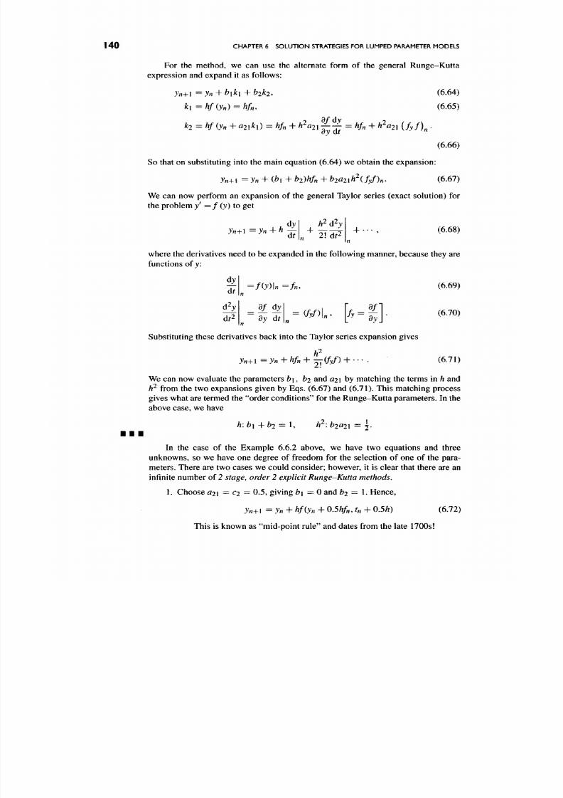
8/17/2019 Process Modelling and Model Analysis-Hangos-Cameron
http://slidepdf.com/reader/full/process-modelling-and-model-analysis-hangos-cameron 157/560
140
CHAPTER 6 SO LU TIO N STRATEGIES FOR LUMPED PARAMETER MODELS
For the method, we can use the alternate form of the general Runge-Kutta
expression and expand it as follow s:
yn+l =yn+b\k\ +b2k2,
k\ = hf (y„) = Itfn,
ki
-
hf
(y„ + azi^ l) = hfn
+
' ' ^ « 2 l ^ ^ = hf„ + h^a2x
(fyf)^
.
(6.64)
(6.65)
(6.66)
So that on substituting into the main equation (6 .64) we obtain the expansion:
yn+l =
yn + ( 1 + b2)hfn
+ b2a2ih^(fyf)„.
(6.67)
We can now perform an expansion of the general Taylor series (exact solution) for
the problem
y'
=:f(y)
to get
yn+{ ^yn + h
dy
df ^ 2 d ^
+
•
(6.68)
where the derivatives need to be expanded in the following manner, because they are
functions of _y:
dy
dt
d'^y
d ^
= f(y)\n =fn,
^ d y
dy dt
^-m„,
[/.= ].
Substituting these derivatives back into the Taylor series expansion gives
yn-\-l = J/i + hfn 4-
—(fyf)
+ ' ' •
(6.69)
(6.70)
(6.71)
We can novv evaluate the parameters
b{
, ^2 and
21
by matching the terms in
h
and
h^
from the two expansions given by Eqs. (6.67) and (6.71). This matching process
gives what are termed the "order
conditions"
for the Runge-Kutta parameters. In the
above case, we have
h:
b\ -\-b2 =
1,
h
:
hiaix = j -
In the case of the Example 6.6.2 above, we have two equations and three
unknowns, so we have one degree of freedom for the selection of one of the para
meters. There are two cases we could consider; however, it is clear that there are an
infinite number of 2 stage, order 2 explicit Runge- K utta methods.
1. Choose
a2\ =
C2
=
0.5, giving
bi =0
and ^2 = 1- Hence,
yn+\ =yn+ hfiyn
+
0.5hfn, tn + 0.5h)
(6.72)
This is known as "mid-point rule" and dates from the late 1700s
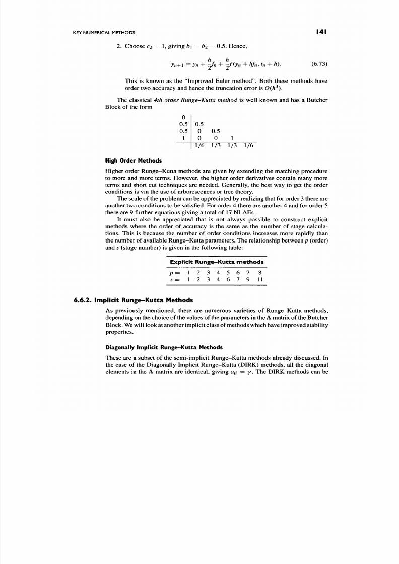
8/17/2019 Process Modelling and Model Analysis-Hangos-Cameron
http://slidepdf.com/reader/full/process-modelling-and-model-analysis-hangos-cameron 158/560
KEY NUMERICAL METHODS 1 4 1
2. Choose C2 = 1, giving by = b2 = 0.5. Hence,
yn+l ^yn + :^fn
+
^f(yn
+
hfn, h
+
h).
(6.73)
This is known as the "Improved Euler method". Both these methods have
order two accuracy and hence the truncation error is
The classical 4th order Runge-Kutta method is well known and has a Butcher
Block of the form
0
0.5
0.5
1
0.5
0
0
1/6
0.5
0 1
1/3 1/3 1/6
High Order Methods
Higher order Rung e-Kutta methods are given by extending the matching procedure
to more and more terms. However, the higher order derivatives contain many more
terms and short cut techniques are needed. Generally, the best way to get the order
conditions is via the use of arborescences or tree theory.
The scale of the problem can be ap preciated by realizing that for order 3 there are
another two co nditions to be satisfied. F or order 4 there are another 4 and for order 5
there are 9 further equations giving a total of 17 NLAEs.
It must also be appreciated that is not always possible to construct explicit
methods where the order of accuracy is the same as the number of stage calcula
tions. This is because the number of order conditions increases more rapidly than
the number of available Runge-Kutta parameters. The relationship between p (order)
and 5 (stage num ber) is given in the following tab le:
Expl ic i t Runge-Kutta methods
/ ? = 1 2 3 4 5 6 7 8
5 = 1 2 3 4 6 7 9 11
6.6.2. Implicit Runge-Kutta Methods
As previously mentioned, there are numerous varieties of Runge-Kutta methods,
depend ing on the cho ice of the values of the parameters in the A m atrix of the Bu tcher
Block. We will look at another implicit class of methods w hich have improved stability
properties.
Diagonally Implicit Runge-Kutta Methods
These are a subset of the semi-implicit Runge-Kutta methods already discussed. In
the case of the Diagonally Implicit Runge-Kutta (DIRK) methods, all the diagonal
elements in the A matrix are identical, giving
an — y .
The DIRK methods can be

8/17/2019 Process Modelling and Model Analysis-Hangos-Cameron
http://slidepdf.com/reader/full/process-modelling-and-model-analysis-hangos-cameron 159/560

8/17/2019 Process Modelling and Model Analysis-Hangos-Cameron
http://slidepdf.com/reader/full/process-modelling-and-model-analysis-hangos-cameron 160/560
KEY NUMERICAL METHODS 143
Here we know that b\ = I, However, we can choose y to be either 0.5 or 1.0. If y is
1.0 then we have an order one method, which is in fact the Backward Euler method
• I • If y is 0.5 then the order can be greater than one.
Solving the Implicit Formulae
Because the DIRK methods are implicit, it involves solving a set of n equations for
each stage calculation using an iterative method . The most comm on way of doing this
is via a Newton iteration. We can see that an implicit stage calculation for a DIRK
method looks like
y = hyf(y)-^^, (6.78)
A New ton iteration applied to this equation gives the following iteration:
(I -
hyj) Ay^y = hyf
( j ^ •)
-^ x/r -
j ^
-. (6.79)
Here, J is the Jacobian of the right-hand side of the system equations. Since y is the
same from one stage calculation to the next, it is wise to use the factored iteration
matrix (I —
hyj)
for as long as possib le. This linear system is usually solved using
some form of Gaussian factorization technique.
6.6.3. Estimating Local Errors
A major problem with Runge-Kutta methods is the stepsize control and error es
timation in the solution. Many codes use fixed steplength implementation but this is
inefficient and can produce unacceptable results. There are two basic approaches for
estimating error per step:
(a) Extrapolation: where the step is repeated by using two half steps and the
resultant solution compared with that of the single step.
(b) Embedding: where
two
method s of differing order
are
used over
the
step and the
difference used as an error estimator. This is the technique used in many code s
such as MA TLA B's OD E23 (2nd + 3rd order methods) or ODE45 (4th + 5th
order methods).
Extrapolation
This is based on the Richardson extrapolation technique. Here, the integration from
tfi-i to tn is done twice. A full step is taken to give a solution y^^h ^^^ then two steps
of
h/2
are taken to give another solution at the end of the step designated by
yn,h/2-
The numerical solution of order p with step h can be written as
yn,h = yitn) + hP^^iritn) + OihP^^), (6.80)
where
if(tn)
is the principal error term of the pth o rder formula.
For two steps at h/2 we obtain
yn,h/2 = yitn) + 2 (^\ ir{tn) + 0{hP^^). (6.81)
8/17/2019 Process Modelling and Model Analysis-Hangos-Cameron
http://slidepdf.com/reader/full/process-modelling-and-model-analysis-hangos-cameron 161/560
144 CHAPTER 6 SOLUTIO N STRATEGIES FOR LUMPED PARAMETER MODELS
If we want to estimate the principal error in the last equation, i.e. the more accurate
solution
yn,h/2^
we can subtract the two expressions and rearrange to get an estimate
of the error
{En)'.
^« = —
' ^ T T i
— •
( - ^
This error can now be added to the more accurate solution to get an "extrapolated"
or more accurate value:
y^^ynJi/l+En. (6.83)
• • • EXAMPLE 6.6.4 (Error estimator for second-order Run ge-K utta method). In
applying the extrapolation technique to a second-order Runge-Kutta method the
error estimator would be
J. iy,nM-ynMI2) , , o . ,
E n = — ,
(6.84)
• • • since
p
—
2.
Embedding
In this case, each step is integrated using a /?th order method as well as a (p -h l)th
order method. The error in the lower order can then be estimated as
En = \\y^n^^-yh^
It
is
then possible
to
proceed w ith either solution although it
is
normally advisable
to use the higher order method which will be more accurate.
The advantage of embedding is that Runge-Kutta methods can be constructed
so that the two solutions can be obtained by the same Butcher block. Hence, it can
be a very cheap way of getting an error estimate compared with the extrapolation
technique.
6.6.4. Controlling Step Size Automatically
Using either extrapolation or embedding, we can obtain an error estimator En. If we
have a user specified error tolerance per step (r), we can compare the two and then
decide how to chang e the steplength to control error automatically. It
is
clear that if the
error estimate is smaller than our desired error, then we can increase the steplength.
The reverse is true. However, by how much do we change the steplength? This is
clearly controlled by the accuracy (order) of the method being used. We can analyse
this situation and develop a strategy to change steplength as follows.
The error in a Runge-Kutta method of order p at tn is given by
^ . = /^^V(^n ) + 0( / i^ +^ ). (6.85)
Consider that the new steplength is related to the previous step by
hn^\=qhn.
(6.86)

8/17/2019 Process Modelling and Model Analysis-Hangos-Cameron
http://slidepdf.com/reader/full/process-modelling-and-model-analysis-hangos-cameron 162/560
KEY NUMERICAL METHODS
145
If we assume that the value of
\lr(t)
does not change significantly over the step, then
the principal error term for the next step becomes:
(qhnr^^^{tn) + 0{hP'^^y (6.87)
We know that we want the error on the next step to be less than or equal to the
tolerance
T,
so w e can demand that
r =
(qhnf^^^lfitn)
+
O
(/r^+^) , (6.88)
and thus,
/ ^ ^ = ^ , (6 .8 9)
En
/ ^ \1 / (P+1)
hn^^=^n{ — ]
. (6.90)
In practice, this new value hn-\-\ is multiplied by a safety margin of 0.8-0 .9 to addres s
the basic assumption of constant \lr(tn) in developing the technique.
6.6.5. Linear Multi-step Methods and their Solution
The Adams-Bashforth and Adams-Moulton methods are LMMs which require iter
ative solution techniques to solve the implicit difference equations. As previously
noted in Section 6.3.1 we can write the methods as
k
k
J2
ccjyn-^j
= hJ2
Pjfn+j (6.91)
if
Pl^
=0
then the methods are
explicit,
if ^^ ^ 0 then the method s are implicit.
In the above equation we need to solve for yn-^-k- We can rewrite this in generic
form as
y = hyfiy) + lA, (6.92 )
where
x/r
contains all the past (known) information.
There are now two basic ways of solving this nonlinear system.
Functional Iteration
We have
/ + =
hyfiy^)
+
i/f,
(6.93)
and we iterate to convergence so that
| | / + l _ / | | < ^ . (6.94)
However, we know that this iterative technique will only converge when
\hyL\
<
1, (6.95)

8/17/2019 Process Modelling and Model Analysis-Hangos-Cameron
http://slidepdf.com/reader/full/process-modelling-and-model-analysis-hangos-cameron 163/560
146
CHAPTER
6
SOLU TION STRATEGIES FOR LUMPED PARAMETER MODELS
where
L
is the Lipschitz constant of/, which is given by || 9/ /9 y| |. D epending on the
value of L, the steplength h will be bounded by \/yL. In the case of a "stiff" problem,
L
is large and hence this iterative technique limits
h.
Newton Iteration
A m ore robust method for large h is the New ton-like iteration wh ich when applied to
the method yields
( I - / zy j )A /+* =^lf^ hyf(y^) - y\ (6.96)
where
J = — ; I = unit matrix. (6.97)
dyj
Normally, this is used in production codes for Adam's methods although an option
to use functional interaction is also included for solving "stab le" problems, since this
avoids the use of a Jacobian matrix.
Error Estimates and Step-Changing in LMMs
The derivation of LMMs can be done via Taylor series matching. The constant
Cp^\
can be identified as the principal error constant and the local truncation error can be
written in the form
y{tnu) -
yn+k
= Cp^xhP^^y^^^Htn)
+
OihP^^),
(6.98)
where
y^ ^
is the pth de rivative of
y .
Hence, for an explicit and implicit method we
can write
Llyity, h] = Cp^ihP'^^y^^^Ht)
+ 0(/i^+^), (6.99)
L*\y{t);
ft]
= Cp*^xhP*^^y^*^^\t)
+
0{hP^^),
(6.100)
If we assume that the order of the methods is the same (p =/?*), then we can
write that
Cp^lhP+^y^^^\tn)
=
yitnu) - yflk
+
O ' ^^)
(6.101)
and
Cp^ihP^^y^^^\tn) = yitnu) - J S + ^('^^^^>' (6-102)
where y^^^j^ is the predicted value of the solution by the explicit method and
y^^^^^
is
the final value computed by its implicit counterpart. On subtracting and rearranging
we can obtain an estimate of the principal truncation error for the implicit method.
C,,lf y '\tn)= ; r - ^ - ( « - e ) • (6.103)
This is known as Milne's device for estimation of error.

8/17/2019 Process Modelling and Model Analysis-Hangos-Cameron
http://slidepdf.com/reader/full/process-modelling-and-model-analysis-hangos-cameron 164/560
KEY NUMERICAL METHODS 147
We can also obtain the principal error term for the explicit method as
We can thus use previous error estimator as a means of controlling error in the cor
rector (implicit) equation by using the difference between the predicted value of the
solution y^^\ and the final value
y '"^
from the corrector. Henc e, the error estimate En
is given by
E, = ^E±l^-(y(m)
_
y(0)y
(6J05)
Norm ally, we wan t to control the error per step so that En < r. We would like to
adjust the steplength h to achieve this error. Hence, we can write that
Cp+lCdy^^^\tn)C^En
(6.106)
and on the next s tep we want to have the error Enew — En so that
Cp^iCwy^^^Htn) = X
(6.107)
£: = i ( 3 ; ( ' ^ ) - / 0) ) . (6.108)
Using the previous expressions we obtain
in a similar manner to the Runge-K utta m ethods.
\ l / (P+l )
K^^ = K\A — \ (6.109)
EXAMPLE 6.6.5 (Error estimator for a linear mu lti-step pair). Con sider the use
of an Euler method as a predictor and the Backward E uler method as a c orrector as a
means of controlling error automatically.
We know that for the Euler method that C^+i = ^ and for the Backward E uler
method
C -j-i
= —
^
so that the principal error estimate for the backward Euler
method is
£ „ = ^ ( / ' « ) - / 0 ) ) (6.110)
and the step change mechanism is
/ ^ \ 1/(^+1)
/ new =/^ old ( ^ ) • (6 .11 1)
In practice we are normally
conservative
and choose to take the new step as 80-9 0%
of the calculated value.
Stability Regions of the Adams Methods
Both Adams-B ashforth and Adams-M oulton methods have limited stability regions.
Typical stability regions are smaller than the equivalent order Runge-Kutta methods.
This makes the methods inappropriate for the solution of
"stiff"
problems. Figure
6.7 shows the stability regions in the hk-plane for several different order Adams
methods.
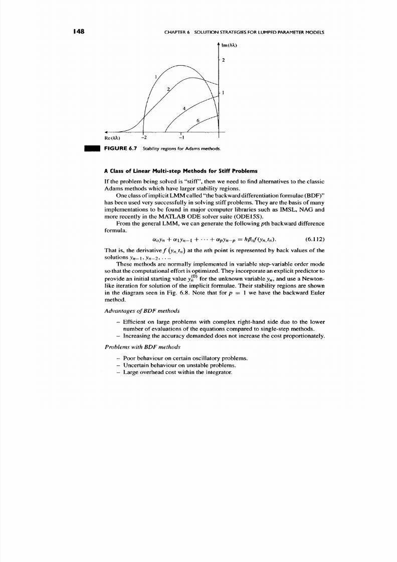
8/17/2019 Process Modelling and Model Analysis-Hangos-Cameron
http://slidepdf.com/reader/full/process-modelling-and-model-analysis-hangos-cameron 165/560
148
CHAPTER 6 SOLUTION STRATEGIES FOR LUMPED PARAMETER MODELS
f
lm(hX)
RtihX) -2 -1
F I G U R E 6 .7 Stability regions fo r Adams methods.
A Class of Linear Multi-step Methods for Stiff Problems
If the problem being solved is
"stiff",
then we need to find alternatives to the classic
Adams methods which have larger stability regions.
One class of implicit LMM called "the backward differentiation formulae (B DF )"
has been used very successfully in solving stiff problem s. They are the basis of many
implementations to be found in major computer libraries such as IMSL, NAG and
more recently in the MATLAB O DE solver suite (0D E1 5S) .
From the general LMM, we can generate the following
pih
backward difference
formula.
(Xoyn + a i J / i - 1 4 - h O lpyn-p = hPofiynJn)-
(6.112)
That is, the derivative/
(ynjn)
at the nth point is represented by back values of the
so lu tion s j „ _ i , j „ _ 2 , . . . .
These methods are normally implemented in variable step-variable order mode
so that the compu tational effort is optimized. They inco rporate an explicit predictor to
provide an initial starting value yfi for the unknown variable j „ , and use a New ton
like iteration for solution of the implicit formulae. Their stability regions are shown
in the diagram seen in Fig. 6.8. No te that for /? = 1 we have the backward Euler
method.
Advantages of BDF methods
-
Efficient on large problem s with complex right-hand side due to the lower
number of evaluations of the equations compared to single-step methods.
- Increasing the accuracy demand ed does not increase the cost proportionately.
Problems with BDF methods
-
Poor behaviour on certain oscillatory problems.
- Uncertain behaviour on unstable problem s.
- Large overhead cost within the integrator.

8/17/2019 Process Modelling and Model Analysis-Hangos-Cameron
http://slidepdf.com/reader/full/process-modelling-and-model-analysis-hangos-cameron 166/560
DIFFERENTIAL-ALGEBRAIC EQUATION SOLUTION TECHNIQUES
149
Re(R ) - 4 - 2 ' 2 4 Re(R )
F I G U R E 6 . 8 Stability regions fo r the BDF methods.
Stability regions of the BDF methods are substantially larger than the Adams
methods as seen in Fig. 6.8. Note that the stable region around the imaginary axis
becom es substantially less
as the
order increases . Higher order
BDF
methods approach
A{a)-stability
regions and are less attractive when the solutions are oscillatory and
thus hk would lie near the imaginary axis.
6.7. DIFFERENTIAL-ALGEBRAIC EQUATION SOLUTION TECHNIQUES
Differential-algebraic equation solution techniques are an extension of standard
ordinary differential ODE solvers. However, there are some very significant dif
ferences between the two types of solution procedures, namely index problems and
consistent initialization issues. Recall that the general form of a DAE system is
0 = g(y,zj).
6.7 .1 .
Substitute for Algebraic Variables
One simplistic approach, which can be used on small systems with the appropriate
structure, is to substitute the algebraic variables
z
into the right-hand sides of the
differential e qu ati on s/ and eliminate
z
completely. This procedure results in a set of
ODEs with no algebraic constraints. The following example shows how this can be
done on a simple tank problem.
• • • EXAMPLE 6.7.1 (Elimination of algebraic variables to get an OD E set). Con
sider the equations which describe the simple tank dynamics given in Example 6.1.2.
These are given as one ODE and four algebraic constraints. The equations are
Ah
- = ( F i - F 2 ) / A ,
at
Fx = Cyy/Pi - P2,
(6.113)
(6.114)
8/17/2019 Process Modelling and Model Analysis-Hangos-Cameron
http://slidepdf.com/reader/full/process-modelling-and-model-analysis-hangos-cameron 167/560
I 50 CHAPTER 6 SOLUTIO N STRATEGIES FOR LUMPED PARAMETER MODELS
F2 = Cw^P2-P3. (6.115)
P2 = Po-^P8h.
(6.116)
In this case, we can observe that the expression for
P2
in
Eq.
(6.116) can be substituted
into Eqs (6.114) and (6.115) to eliminate P2. Following this, we can substitute the
expressions for F{ and F2 into the ODE to get the final single OD E:
• • •
^ = \[Cw{P\ -Po- Pghr2 - Cv(Po + Pgh - P^r^l (6.117)
This approach appears to be useful, however there are two major drawbacks:
(a) It is often not poss ible to solve for z in terms of the differential variables y,
(b) When there are many algebraic variables, the substitution task becomes
almost impossible.
It has also been shown that in special circumstances it is not wise to substitute to
remove the algebraic co nstraints as information is lost.
6.7.2. Explicit ODE Solver
Here we can use an explicit ODE solver and solve the algebraic equation set each
time the right-hand side of the ODEs are evaluated.
This approach attemp ts to decouple the algebraic and differential systems, using
a simple explicit (and hence low computational cost) solver for the ODEs and then
iterate to solve the accom panying algebraic system. Con sider the general DAE system
given by
yfiyzj), (6.118)
0 = g(y,z,t).
(6.119)
In this case, the differential variables
y
at time tn w ould be known by the explicit
integrator and hence are usually passed to the function evaluation routine to obtain
the function va lue /„. Before attempting to evalua te/^ it will be necessary to evaluate
Zn by solving Eqs (6.119) for the unknowns Zn- Having both j„ and Zn allows the
evaluation of/^. This is then used to advance to the new value of j„^_i.
Again we can illustrate this on the previous example.
EXAMPLE 6.7.2 (Using an explicit ODE solver and independent algebraic
solver). If we consider the simple tank problem again, w e can see that the only
state or differential variable is h. The unknown values in the right-hand side of the
ODE are F \ and
F2
and these come from the solution of the three algebraic equations.
Hen ce, having the value of the liquid height
h
at time tn from the explicit ODE solver,
we can proceed in the following steps:
• Solve the algebraic system of three equations for F\, F2 and P2.
• Evaluate the right-hand side of the differential equation.
• Return to the integrator to update the value of liquid height at time
tn-\-\.
• Go back to the first step.
8/17/2019 Process Modelling and Model Analysis-Hangos-Cameron
http://slidepdf.com/reader/full/process-modelling-and-model-analysis-hangos-cameron 168/560
DIFFERENTIAL-ALGEBRAIC EQUAT ION SOLUT ION TECHNIQUES I 5 I
The problems with this approach
are
(a) The need to solve a separate set of algebraic equations at each step.
(b) The decoupling of differential and algebraic v ariables.
(c) The increased load when using higher order methods like the Ru nge-K utta
techniques. This is a lot of work per step due to the number of internal stage
calculations, which require the solution of the algebraic subsystem.
(d) The technique is very inefficient for "stiff" problems.
6.7.3. Using Implicit Differential-Algebraic Equation Solvers
Here, we use an implicit solver which simultaneously solves the ODEs and the al
gebraic equations in a coupled manner. Th is approach is the preferred option to cover
most circumstances.
It
requires
a
modification
of
the standard implicit ODE code.
For example any implicit method , be it Ru nge -K utta or Backw ard Differentiation
Formulae (BD F) can be w ritten
as
y
=
hyf(y)
+ ^|r,
(6.120)
where
h
is the current steplength,
y
is a constant related to the method and ^ is a vector
of known information. Here, y is being solved to advance to the next solution point.
Using this formula, we can solve both the states and algebraic variables simultaneously
using a typical N ewton iteration to give
r*
.k+l
( A Z ) =-f(y'Z,tf, (6.121)
where the Jacobian T is
r*
l-hydf/dy -hydf/dz
-hydg/dy -hydg/dz
(6.122)
representing the combined ODE and algebraic system. The right-hand side function
value
in
the Newton iteration shown
in
Eq. (6.121)
is
given
by
_f_\ ^ + hyf(y',z',t)-y'
1
and the increment vectors Ay and Az for differential and algebraic variables are
defined
as
^yk+\
^yk+l
_yk (6 124)
A z ^ + ^ = z ^ + ^ - z ^ ( 6 . 1 2 5 )
This
set of
algebraic equations
is
solved
at
each step, requiring
the
calculation
of a Jacobian matrix and the subsequent iteration of the Newton method to some
convergence criterion.
This approach (and slight variations of it) is the most widely used technique
for coupled solutions.
A
number
of
well known codes
are
available
to
handle DAE

8/17/2019 Process Modelling and Model Analysis-Hangos-Cameron
http://slidepdf.com/reader/full/process-modelling-and-model-analysis-hangos-cameron 169/560
I 52 CHAPTER 6 SOLUTIO N STRATEGIES FOR LUMPED PARAMETER MODELS
systems in this way. The most prominent of the BDF based routines is the DASSL
code by Petzold [46] and the suite of routines by Barton and co-wo rkers at MIT [47].
Other codes based on variants of Runge-Kutta methods are also available such as
DIRK (Cameron [48]) and RadauS (Hairer etai [49]) and ESDIRK [50]. The widely
available MATLAB system has a suite of routines suitable for solving DAE systems
using codes like 0D E1 5S .
6.7.4. Exploiting Equation Structure
The final technique exploits the algebraic equation structure and seeks to reduce the
problem to the smallest possible coupled DAE set or to reduce the problem to a series
of simple sequential algebraic calculations before evaluating the ODEs
Here, we analyse the equations to find a partition and precedence order in the
algebraic set. This technique is used extensively to decompo se large sparse problem s
into smaller more tractable subproblems which can be solved sequentially. The sam e
technique is applicable to the algebraic subset of the DAE problem with the intention
to find partitions and a precedence order which makes the algebraic system a fully
sequential calculation. After c arrying out this analysis, it might be possible to structure
the original model in sequential form, so that each algebraic variable is a simple
explicit substitution, knowing only the differential variables
y
and any previously
calculated algebraic variables. The calculation sequence could be
zi=qi(y),
(6.126)
Z2 = q2(y,zi), (6.127)
* (6.128)
Zn = qniy. Zn-\, Zn-2, • • - , Z l) , (6.129)
with the ODEs being
y = / ( j , ^ , 0 . (6.130)
In some cases, certain algebraic equations form coupled sets and must be solved
simultaneously. This is a function of the original problem structure. This technique
often shares the advantages of the simultaneous DAE solver with some efficiency in
solution due to the algebraic structuring.
Partitioning and Precedence Ordering in Algebraic Systems
The key to carrying out this structural analysis is contained in two principal steps:
• establishing an output assignment for the equation system,
• generating the partitions and precedenc e order.
This analysis is carried out on the algebraic subset of the DAEs given by Eqs
(6.118) and (6.119). The first step seeks to assign to each algebraic equation an
"output" variable which is calculated knowing all other variables in the equation.
This is done for all equations.
The basis of the analysis is a structural representation of the equation set which
identifies which variables occur in each equation. To do this, we can construct an
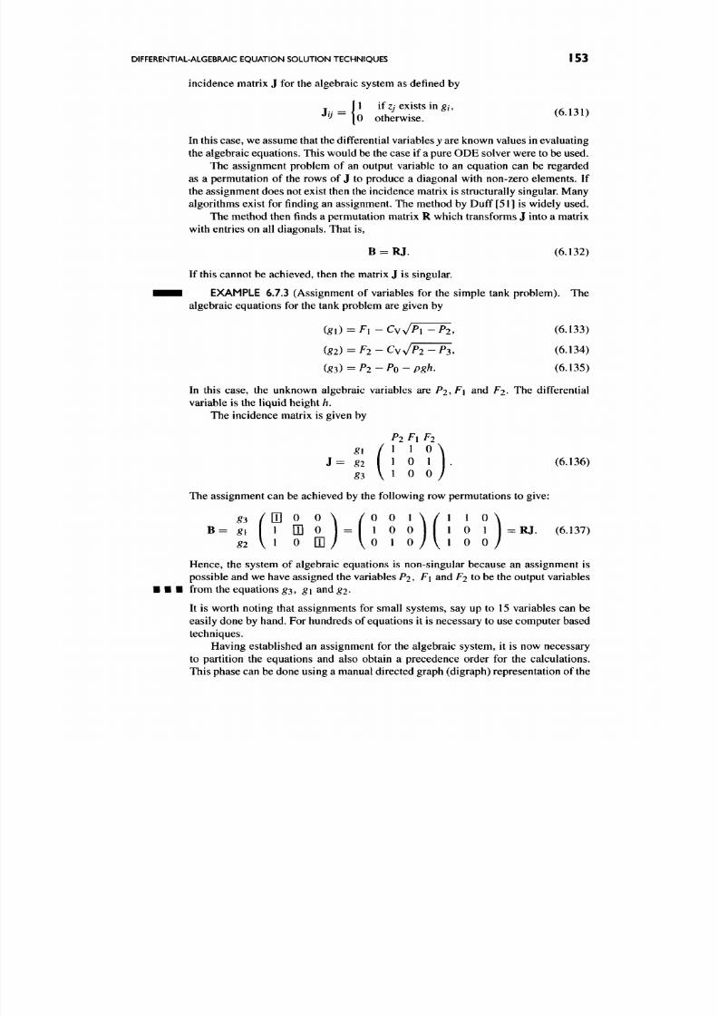
8/17/2019 Process Modelling and Model Analysis-Hangos-Cameron
http://slidepdf.com/reader/full/process-modelling-and-model-analysis-hangos-cameron 170/560
DIFFERENTIAL-ALGEBRAIC EQUATION SOLUTION TECHNIQUES
I 53
incidence matrix J for the algebraic system as defined by
In this case, we assu me that the differential variables
y
are known values in evaluating
the algebraic equations. This would be the case if
a
pure OD E solver were to be used.
The assignment problem of an output variable to an equation can be regarded
as a permutation of the rows of J to produce a diagonal with non-zero elements. If
the assignment d oes not exist then the incidence m atrix is structurally singular. Many
algorithms exist for finding an assignm ent. The method by Duff [51] is widely used.
The method then finds a permutation matrix R which transforms J into a matrix
with entries on all diagonals. That is,
B = R J. (6.132)
If this cannot be achieved, then the m atrix J is singular.
• • 1 EXAMPLE 6.7.3 (Assignment of variables for the simple tank problem). The
algebraic equations for the tank problem are given by
(g\) = Fi-Cw^Pr^^,
(6.133)
(82) = F2- Cyy/P2-P 3.
(6.134)
(g3) = P2-Po-P8h, (6.135)
In this case, the unknown algebraic variables are P2» ^l ^^d F2. The differential
variable is the liquid height
h.
The incidence matrix is given by
P2
Fi F2
^1 / 1 1 0 \
J = g2 1 0 1 . (6.136)
^3 \ 1 0 0 /
The assignment can be achieved by the following row permutations to give:
ffl
B= gx \ I
[ I ] 0 j = | 1 0 0 | | 1 0
1 | = R J .
(6.137)
Hence, the system of algebraic equations is non-singular because an assignment is
possible and we have assigned the variables
P2, F\
and
F2
to be the output variables
• • from the equations
g3 ,
g\ and^2-
It is worth noting that assignments for small systems, say up to 15 variables can be
easily done by hand. For hundreds of equations it is necessary to use computer based
techniques.
Having established an assignment for the algebraic system, it is now necessary
to partition the equations and also obtain a precedence order for the calculations.
This phase can be done using a manual directed g raph (digraph) representation of the
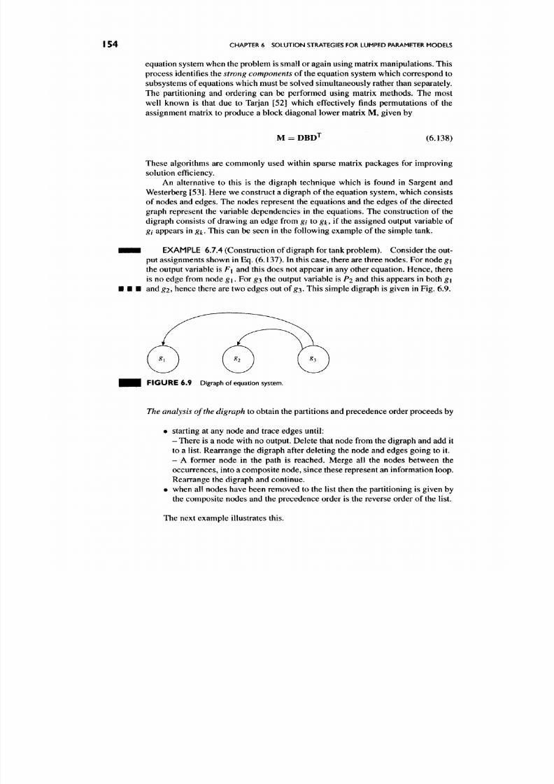
8/17/2019 Process Modelling and Model Analysis-Hangos-Cameron
http://slidepdf.com/reader/full/process-modelling-and-model-analysis-hangos-cameron 171/560
I 54
CHAPTER
6
SOLUTIO N STRATEGIES FOR LUMPED PARAMETER MODELS
equation system w hen the problem is small or again using matrix man ipulations. This
process identifies the
strong components
of the equation system which correspond to
subsystems of equations w hich must be solved simultaneously rather than separately.
The partitioning and ordering can be performed using matrix methods. The most
well known is that due to Tarjan [52] which effectively finds permutations of the
assignment matrix to produce a block diagonal lower matrix M, given by
M = DB D^ (6.138)
These algorithms are commonly used within sparse matrix packages for improving
solution efficiency.
An alternative to this is the digraph technique which is found in Sargent and
Westerberg [53 ]. Here we cons truct a digraph of the equation system , which co nsists
of nodes and edges. The nodes represent the equations and the edges of the directed
graph represent the variable dependencies in the equations. The construction of the
digraph consists of drawing an edge from gi to gk, if the assigned ou tput variable of
gi
appears in
g^.
This can be seen in the following example of the simple tank.
EXAMPLE 6.7.4 (Con struction of digraph for tank problem). Consider the out
put assignments show n in Eq. (6.13 7). In this case, there are three nodes. For node g\
the output variable is
F \
and this does not appear in any other equation. Hence, there
is no edge from node
g \.
For
g^
the output variable is P2 and this appears in both
g\
and g2, hence there are two edges out of ^ 3 . T his simple digraph is given in Fig. 6.9.
F I G U R E 6 . 9 Digraph of equation system.
The analysis of the digraph to obtain the partitions and precedenc e order proceed s by
• starting at any node and trace edges until:
- There is a node with no output. Delete that node from the digraph and add it
to a list. Rearrange the digraph after d eleting the node and ed ges going to it.
- A former node in the path is reached. Merge all the nodes between the
occurrenc es, into a com posite node, since these represent an information loop.
Rearrange the digraph and continue.
• when all nodes have been removed to the list then the partitioning is given by
the compo site nodes and the precedence order is the reverse order of the list.
The next examp le illustrates this.
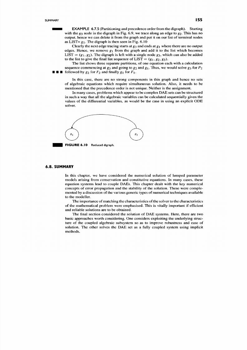
8/17/2019 Process Modelling and Model Analysis-Hangos-Cameron
http://slidepdf.com/reader/full/process-modelling-and-model-analysis-hangos-cameron 172/560
SUMMARY 155
• ^ • 1 EXAMPLE 6.7.5 (Partitioning and precedence order from the digraph). Starting
with the ^3 node in the digraph in Fig. 6.9, we trace along an edg e to gj. This has no
output, henc e we can delete it from the graph and put it on our list of terminal nodes
as LIST= g\. The digraph is then seen in Fig. 6.10
Clearly the next edge tracing starts at
^3
and ends at
g\
where there are no output
edges. Hence, we remove g\ from the graph and add it to the list which becomes
LIST = (^1, ^2)- The digraph is left with a single node ^ 3 , which can also be added
to the list to give the final list sequence of LIST
= {g\,g2,g^).
The list shows three separate partitions, of one equation each with a calculation
sequence commencing at ^3 and going to
g2
and
g \.
Thus, we would solve ^3 for P2
• • • followed by g2 for F2 and finally ^1 for F\.
In this case, there are no strong components in this graph and hence no sets
of algebraic equations which require simultaneous solution. Also, it needs to be
mentioned that the precedence order is not unique. Neither is the assignment.
In many cases, problem s which app ear to be complex DA E sets can be structured
in such a way that all the algebraic variables can be calcu lated sequ entially given the
values of the differential variables, as would be the case in using an explicit ODE
solver.
F I G U R E 6 . 1 0 Reduced digraph.
6.8. SUMMARY
In this chapter, we have considered the numerical solution of lumped parameter
models arising from conservation and constitutive equations. In many cases, these
equation systems lead to couple DAEs. This chapter dealt with the key numerical
concepts of error propagation and the stability of the solution. These were comple
mented by a discussion of the various generic types of numerical techniqu es available
to the modeller.
The imp ortance of matching the characteristics of the solver to the characteristics
of the mathematical problem were emphasised. This is vitally important if efficient
and reliable solutions are to be obtained.
The final section considered the solution of DAE systems. Here, there are two
basic approaches worth considering. O ne considers exploiting the underlying struc
ture of the coupled algebraic subsystem so as to improve robustness and ease of
solution. The other solves the DAE set as a fully coupled system using implicit
methods.
8/17/2019 Process Modelling and Model Analysis-Hangos-Cameron
http://slidepdf.com/reader/full/process-modelling-and-model-analysis-hangos-cameron 173/560
I 56 CHAPTER 6 SOLUTIO N STRATEGIES FOR LUMPED PARAMETER MODELS
6.9. REVIEW QUESTIONS
Q6.1. Describe the characteristics of the two principal classes of problems which
arise from lumped parameter modelling. (Section 6.1)
Q6.2. How do you handle higher order differential systems with the currently
available nu merical routines for first ODEs or DAE s? (Section 6.2.1)
Q6.3. Outline the major categories of OD E solvers and describe their basic char
acteristics. When is it appropriate to use explicit numerical methods? (Section
6.3.1)
Q6.4. Wh at factors contribute to the global error of a numerical solution? What is
the "local error" associated with a numerical solution? What are the key issues in
controlling error? (Section 6.4)
Q6.5. Describe what is meant by the stability of the numerical solution and show
how this is related to both the problem and to the particular numerical method being
used. (Section 6.5)
Q6.6. Describe what is the truncation error of a numerical method and a procedure
by which it can be estimated. (Section 6.4.6)
Q6.7. How is absolute stability of a numerical method desc ribed? What role does it
play in determining the step size of the numerical routine? (Section 6.5.2)
Q6.8. Write down the general formula which describes the Ru nge-K utta methods.
How is this displayed as a Butcher Block? (Section 6.6.1)
Q6.9. Wh at three principal types of Ru nge-K utta methods can be derived? Describe
the characteristics of these metho ds in terms of accuracy, work per step and stability.
(Section 6.6.1)
Q6.10. What methods are typically used for local error control in Runge-Kutta
and LMMs? What advantages and disadvantages exist for the different approaches?
(Section 6.6.3)
Q6.11. Give four ways by which DA E systems could be solved and discuss the
advantages and disadvantages of each. (Section 6.7)
6.10. APPLICATION EXERCISES
A6.1. Consider the following sets of ODEs and convert them to sets of first-order
equations, using the transformations given in Section 6.2.1.
(a)
d M
dudv
. dv
- f — - - - = s m r , — - -\-v -{-u = cos t.
(b)
(c)
dr^ dr dr ' dt
§ - - > ^ > S —
d^y dy dv ^ d^y dv ^
dt^ dt dt dt^ dt
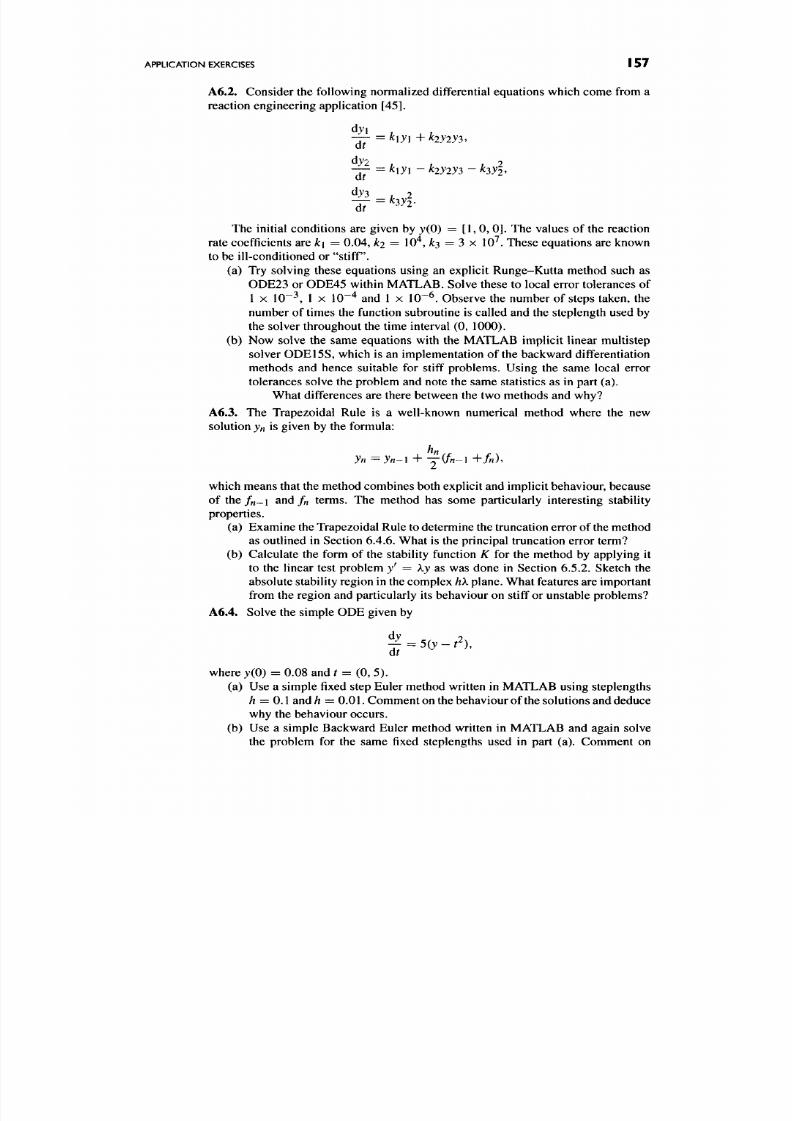
8/17/2019 Process Modelling and Model Analysis-Hangos-Cameron
http://slidepdf.com/reader/full/process-modelling-and-model-analysis-hangos-cameron 174/560
APPLICATION EXERCISES I 57
A6.2. Con sider the following norm alized differential equations which com e from a
reaction engineering application [45].
dy\
— = kiyi-\-k2y2y3^
-^ = km - kiyiy^ - ksyj^
The initial conditions are given by j( 0 ) = [ 1 , 0 , 0 ] . The values of the reaction
rate coefficients are
k\ =
0.04,
k2 =
10"*,
k^ = 3 x
10^. These equations are known
to be ill-conditioned or "stiff".
(a) Try solving these equations using an explicit Runge-Kutta method such as
OD E23 or O DE45 within M ATLA B. Solve these to local error tolerances of
1 X 10~^, 1 X lO"'^ and 1 x 10~^. Observe the number of steps taken, the
number of times the function subroutine is called and the steplength used by
the solver throughout the time interval (0, 1000).
(b) Now solve the same equations with the MATLAB implicit linear multistep
solver 0DE15S, which is an implementation of the backward differentiation
methods and hence suitable for stiff problems. Using the same local error
tolerances solve the problem and note the same statistics as in part (a).
What differences are there between the two methods and why?
A6.3. The Trapezoidal Rule is a well-known num erical method where the new
solution
yn
is given by the formula:
yn=yn-\
+ y ( ^ - l + / / i ) ,
which means that the method combines both explicit and implicit behaviour, because
of the/;i_i and/n terms. The method has some particularly interesting stability
properties.
(a) Exam ine the Trapezoidal Rule to determine the truncation error of the method
as outlined in Section 6.4.6. What is the principal truncation error term?
(b) Calculate the form of the stability function
K
for the method by applying it
to the linear test problem y = Xy as was done in Section 6.5.2. Sketch the
absolute stability region in the complex
hX
plane. What features are important
from the region and particularly its behaviour on stiff or unstable problems?
A6.4. Solve the simple ODE given by
where
y(0)
= 0.08 and
t =
(0, 5).
(a) Use a simp le fixed step Euler method w ritten in MA TLAB using stepleng ths
h = 0.\ and h = 0.01. Comment on the behaviour of the solutions and deduce
why the behaviour occurs.
(b) Use a simple Backward Euler method written in MATLAB and again solve
the problem for the same fixed steplengths used in part (a). Comment on
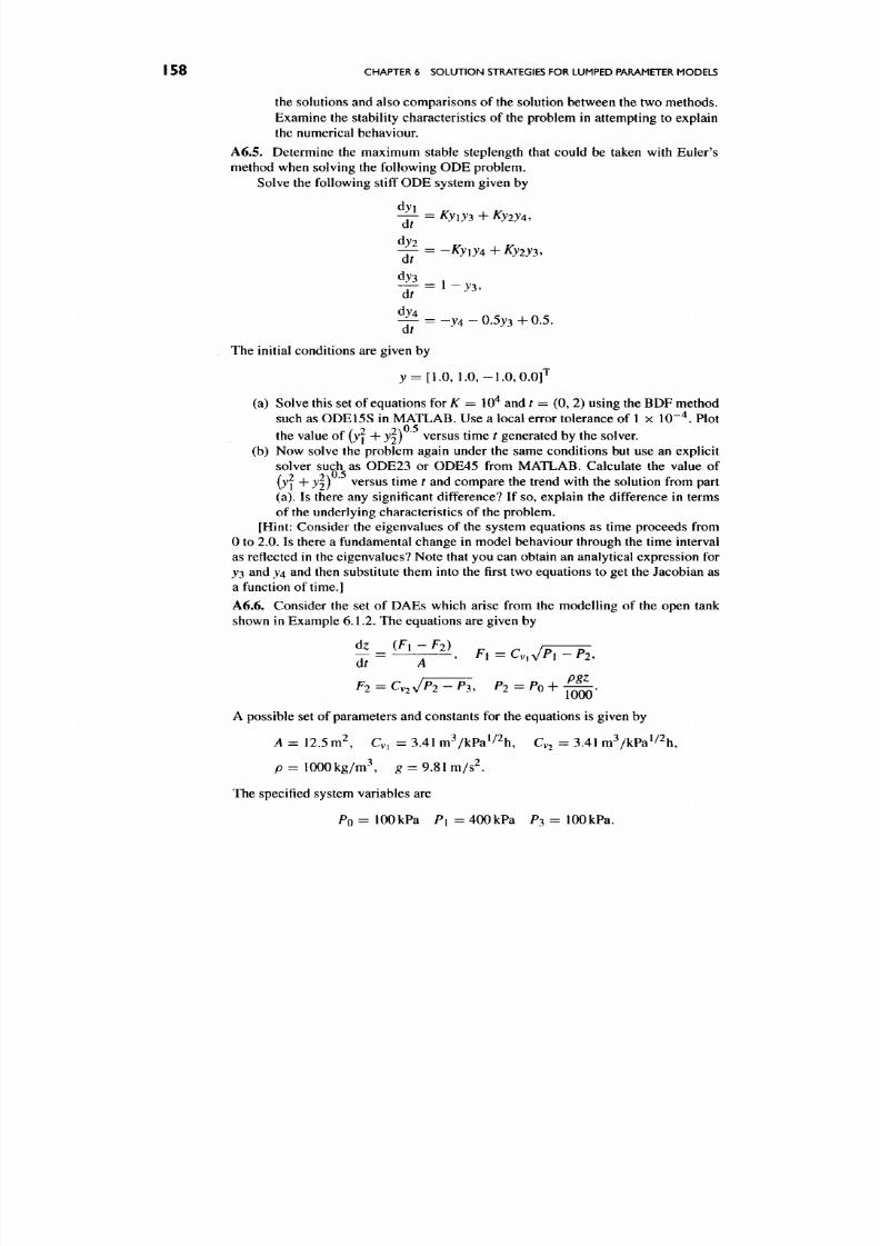
8/17/2019 Process Modelling and Model Analysis-Hangos-Cameron
http://slidepdf.com/reader/full/process-modelling-and-model-analysis-hangos-cameron 175/560
I 58 CHAPTER 6 SOLUTIO N STRATEGIES FOR LUMPED PARAMETER MODELS
the solutions and also comparisons of the solution between the two methods.
Examine the stability characteristics of the problem in attempting to explain
the numerical behaviour.
A6.5. Determine the maxim um stable steplength that could be taken with Euler's
method when solving the following ODE problem.
Solve the following stiff OD E system given by
dvi
—
= Kyiy^ + Ky2y4,
dy2
— = -Kyiy4-\-Ky2y3.
^ = - j 4 - 0 . 5 j 3 + 0 . 5 .
The initial conditions are given by
j = [1.0, 1.0,-1.0,0.0f
(a) Solve this set of equations for
K
= 10" and
t =
(0, 2) using the BD F method
such as 0DE 15 S in MATLAB . Use a local error tolerance of 1 x lO""^. Plot
the value of [y ^ + } 2) versus time t generated by the solver.
(b) Now solve the problem again under the same conditions but use an explicit
solver such as ODE23 or ODE45 from MATLAB. Calculate the value of
0 ? + J2) versus time
t
and compare the trend with the solution from part
(a). Is there any significant difference? If so, explain the difference in terms
of the underlying characteristics of the problem.
[Hint: Consider the eigenvalues of the system equations as time proceeds from
0 to 2.0. Is there a fundamental c hange in model behaviour through the time interval
as reflected in the eigenvalues? Note that you can obtain an analytical expression for
^3 and j4 and then substitute them into the first two equations to get the Jacobian as
a function of time.]
A6.6. Consider the set of DA Es which arise from the modelling of the open tank
shown in Example 6.1.2. The equations are given by
dz (F i -F2) r- —
F2 = Cy,y/P2-P3. P2=P0 +
PgZ
1000
A possible set of parameters and constants for the equations is given by
A = 12.5 m^, Cv, = 3.41 m ^k Pa ^/^ h, Cy^ = 3.41 m^kPa^/^h,
p =
1 0 0 0 k g / m ^
g =
9.81 m/s^.
The specified system variables are
Po =
100 kPa P i
=
400 kPa P3 = 100 kPa.

8/17/2019 Process Modelling and Model Analysis-Hangos-Cameron
http://slidepdf.com/reader/full/process-modelling-and-model-analysis-hangos-cameron 176/560
APPLICATION EXERCISES I 59
(a) Solve the equation set by converting it to a pure OD E problem and then use a
simple Euler method or explicit Runge-K utta method to solve the equation.
Solve for local error tolerances of 1 x 10~^, 1 x 10~^ and 1 x 10~^ and note
the execution time and number of function evaluations in MATLAB.
(b) Set up the problem by calling a nonlinear equation solver each time the
differential equations need to be evaluated. This will take the values of
the differential variables and solve for the unknown values of the algebraic
variables.
(c) Use an implicit DAE solver such as the MATLAB routine 0DE15S which
implements the BDF method. Alternatively use a simple Backward Euler
method. Note the performance over a range of local error tolerances.
(d) Carry out the structural analysis of the algebraic equation set and then solve
this sequential followed by the evaluation of the differential equation s.
Comment on the performance of the methods used and their complexity
of setup. For this problem what is the best solution approach?
A6.7. Con sider the model of the evaporator system considered in App lication
Exercise A5.9. The system is shown in Fig. 6.11.
The model equations for the forced circulation evaporator are given by
dLi dXo dPo
pAs-f=Fi-F4-F2, M-f=FiXi-F2X2, C—^=F^-F^,
at at at
Ti =
fl2^2 +
biXi
+ C2, 7 3 = a3P2 +
c^, F4 = ^ "^
7^100 = ^r^^ioo +
CT,
Qioo =
ciq{F\
+ FsXrioo -
T2),
Floo =
6100
UA2{T2, - T2m) 2200 r G200
^ 200 = ri I
TJA
u^ n 17 \7 ' ^201 = ^200 "r 77-T; , ^ 5 = -\— •
[1 + L^A2/(2CpF200)] CpF200 >^
The following seven (7) parameters are specified:
M s , M , C, Cp, X, As,
Uk2'
All constants a/, foy, C} ^ in the thermo-physical correlations are known.
(a) Using the model equations and the evaporator schematic, analyse the equa
tions to see if it is possible to solve the algebraic equations in a sequential
manner. Make use of the digraph analysis to do this.
(b) Give the solution sequence for this structured set of algebraic equa tions.
(c) Give values for the parameters, and solve the model using an appropriate
solver.
A6.8. Con sider the DAE set which was derived from the mod elling of the enclosed
tank with adiabatic compression of gas which was given in Application Exerc ise A4.1.
Look at possible solution techniques for this problem and compare two principal
methods—one based on structuring of the equation set, the other on a direct DAE
solution.
A6.9. Solve the App lication Exercise of A5.7 for various values of the overall heat
transfer coefficient. Investigate a numerical scheme which solves the problem as a
coupled DAE set as well as considering the structuring of the equations and the use
of an ODE solver. Compare the performance of the solution methods.
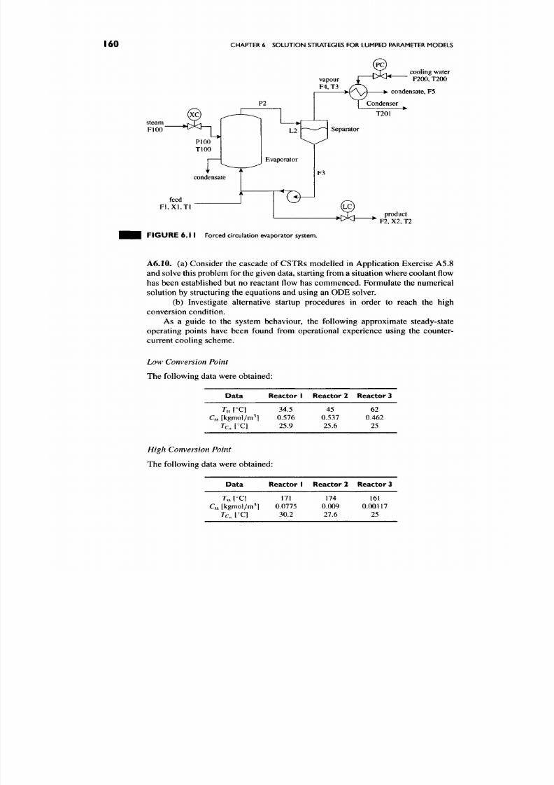
8/17/2019 Process Modelling and Model Analysis-Hangos-Cameron
http://slidepdf.com/reader/full/process-modelling-and-model-analysis-hangos-cameron 177/560
160
CHAPTER 6 SOLUTION STRATEGIES FOR LUMPED PARAMETER MODELS
steam
FlOO
cooling water
F200,
T200
> condensate, F5
feed
F1,X1,T1
F I G U R E 6 . 1 1 Forced circulation evaporator system.
product
F2,
X2,
T2
A6.10. (a) Consider the cascade of CSTR s modelled in Application Exercise A5.8
and solve this problem for the given data, starting from a situation where coolant flow
has been established but no reactant flow has commenced. Formulate the numerical
solution by structuring the equations and using an ODE solver.
(b) Investigate alternative startup procedures in order to reach the high
conversion condition.
As a guide to the system behaviour, the following approximate steady-state
operating points have been found from operational experience using the counter-
current cooling scheme.
Low Conversion Point
The following data were obtained:
D a ta
Reac tor I Reacto r 2 Reacto r 3
Css [kgmol/m^]
TQ . [X]
34.5
0.576
25.9
45
0.537
25.6
62
0.462
25
High Conversion Point
The following data were obtained:
Data
Reac tor I Reac tor 2 Reacto r 3
Css [kgrnol/m"^]
TQ .
[=C]
171
0.0775
30.2
174
0.009
27.6
161
0.00117
25

8/17/2019 Process Modelling and Model Analysis-Hangos-Cameron
http://slidepdf.com/reader/full/process-modelling-and-model-analysis-hangos-cameron 178/560

8/17/2019 Process Modelling and Model Analysis-Hangos-Cameron
http://slidepdf.com/reader/full/process-modelling-and-model-analysis-hangos-cameron 179/560
This Page Intentionally Left Blank
8/17/2019 Process Modelling and Model Analysis-Hangos-Cameron
http://slidepdf.com/reader/full/process-modelling-and-model-analysis-hangos-cameron 180/560
7
DYNAMIC MODELS-
DISTRIBUTED PARAMETER
SYSTEMS
Distributed parameter models, as their name suggests, inc orporate the spatial variation
of states within the balance volum e. They accou nt for situations wh ere the scalar field
of the intensive quantities is both a function of time and position. This could be
a concentration, volume-specific internal energy or temperature. What this means
is that the application of the general conservation equations leads to models which
are represented by partial differential equations (PDEs) in one, two or three spatial
dimensions. This has already been introduced in Chapter 3, which introduced the
general conservation balance over a 3D volume V with a closed boundary surface T.
In this chapter, we develop the basic principles of distributed parameter system
(DPS) modelling by considering the origin of such models, their general form and
the approaches to their construction. A vital part of the model is represented by the
constitutive equations which have been dealt with in Chapter 4.
Another very important aspect of these models is the initial and boundary
conditions which apply to the particular system under consideration. These can
be difficult issues to resolve in some m odelling ap plications.
Following this chapter, we consider the task of solving such systems using a
range of numerical methods.
7 J . DEVELOPMENT OF DPS MODELS
The development of DPS models is illustrated with the simple example of a packed
bed catalytic reactor. The problem statement of the modelling task of the packed bed
tubular catalytic reactor is given as follows:
163
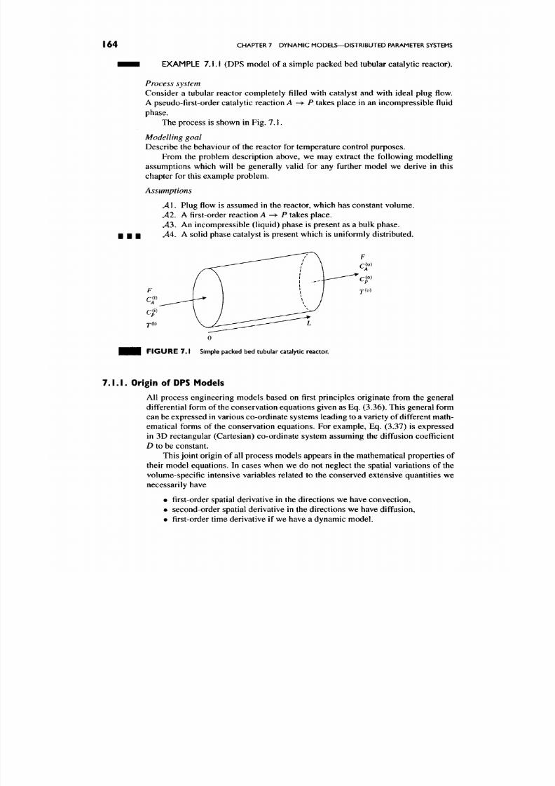
8/17/2019 Process Modelling and Model Analysis-Hangos-Cameron
http://slidepdf.com/reader/full/process-modelling-and-model-analysis-hangos-cameron 181/560
I 64 CHAPTER 7 DYNAMIC MODELS—DISTRIBUTED PARAMETER SYSTEMS
• • • EXAMPLE 7.1.1 (DPS model of a simple packed bed tubular catalytic reactor).
Process system
Consider a tubular reactor completely filled with catalyst and with ideal plug flow.
A pseudo-first-order catalytic reaction
A-^ P
takes place in an inco mpressible fluid
phase.
The process is shown in Fig. 7.1.
Modelling goal
Describe the behaviour of the reactor for temperature control purposes.
From the problem description above, we may extract the following modelling
assumptions which will be generally valid for any further model we derive in this
chapter for this example problem.
Assumptions
Al.
Plug flow is assumed in the reactor, which has constant volume.
A2. A first-order reaction A ^- P takes place.
^ 3 . An incom pressible (liquid) phase is present as a bulk phase .
• • • -4" - A solid phase catalyst is present which is uniformly distribu ted.
0
F I G U R E 7 . 1 Simple packed bed tubular catalytic reactor.
7.1 .1 . Origin of DPS Models
All process engineering models based on first principles originate from the general
differential form of the conservation equations given as Eq. (3.36 ). This general form
can be expressed in various co-ord inate system s leading to a variety of different math
ematical forms of the conservation equations. For example, Eq. (3.37) is expressed
in 3D rectangular (Cartesian) co-ordinate system assuming the diffusion coefficient
D
to be constant.
This joint origin of all process mod els appears in the mathem atical properties of
their model equations. In cases when we do not neglect the spatial variations of the
volume-specific intensive variables related to the conserved extensive quantities we
necessarily have
• first-order spatial derivative in the directions we have convection,
• second-order spatial derivative in the directions we have diffusion,
• first-order time derivative if we have a dynam ic mod el.

8/17/2019 Process Modelling and Model Analysis-Hangos-Cameron
http://slidepdf.com/reader/full/process-modelling-and-model-analysis-hangos-cameron 182/560
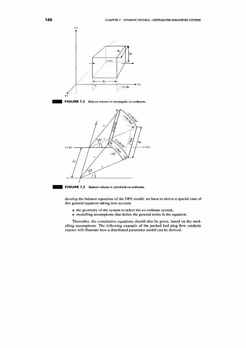
8/17/2019 Process Modelling and Model Analysis-Hangos-Cameron
http://slidepdf.com/reader/full/process-modelling-and-model-analysis-hangos-cameron 183/560
166
CHAPTER 7 DYNAMIC MODELS—DISTRIBUTED PARAMETER SYSTEMS
jc + djc
+z
F I G U R E 7 . 2 Balance volume in rectangular co-ordinates.
z + dz
z + dz
F I G U R E 7 . 3 Balance volume in cylindrical co-ordinates.
develop the balance equations of the DPS model, we have to derive a special case of
this general equation taking into account
• the geometry of the system to select the co-ordinate system ,
• mod elling assum ptions that define the general terms in the equation.
Thereafter, the constitutive equations should also be given, based on the mod
elling assumptions. The following example of the packed bed plug flow catalytic
reactor will illustrate how a distributed parameter model can be derived.
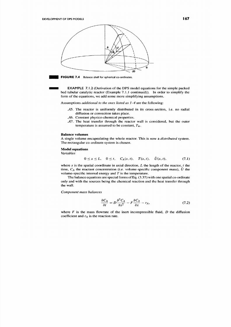
8/17/2019 Process Modelling and Model Analysis-Hangos-Cameron
http://slidepdf.com/reader/full/process-modelling-and-model-analysis-hangos-cameron 184/560
DEVELOPMENT OF DPS MODELS
167
F I G U R E 7 .4 Balance shell for spherical co-ordinates.
EXAMPLE 7.1.2 (Derivation of the DPS model equations for the simple packed
bed tubular catalytic reactor (Examp le 7.1.1 continued)). In order to simplify the
form of the equations, we add some more simplifying assumptions.
Assumptions additional to the ones listed as 1-4 are the following:
^ 5 . The reactor is uniformly distributed in its cross-section, i.e. no radial
diffusion or convection takes place.
A6. Constant physico-chemical properties.
Al.
The heat transfer through the reactor wall is cons idered, but the outer
temperature is assumed to be constant, Tw.
Balance volumes
A single volume encapsulating the whole reactor. This is now a
distributed
system.
The rectangular co-ordinate system is chosen.
Model equations
Variables
0<x<L,
0 < r ,
CA(XJ), T(x,t), U(x,t),
(7.1)
where x is the spatial coordinate in axial direction, L the length of the reactor, t the
time,
CA the reactant concentration (i.e. volume-specific component mass), U the
volume-specific internal energy and
T
is the temperature.
The balance eq uations are special forms of Eq. (3.37) with one spatial co-ordinate
only and with the sources being the chemical reaction and the heat transfer through
the wall.
Component mass balances
dt dx^ dx
(7.2)
where F is the mass flowrate of the inert incompressible fluid, D the diffusion
coefficient and r^ is the reaction rate.

8/17/2019 Process Modelling and Model Analysis-Hangos-Cameron
http://slidepdf.com/reader/full/process-modelling-and-model-analysis-hangos-cameron 185/560
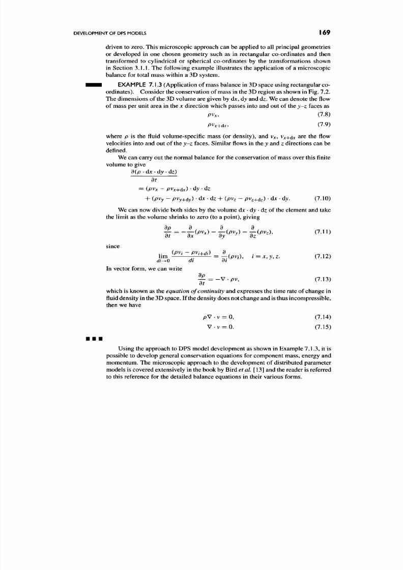
8/17/2019 Process Modelling and Model Analysis-Hangos-Cameron
http://slidepdf.com/reader/full/process-modelling-and-model-analysis-hangos-cameron 186/560
DEVELOPMENT OF DPS MODELS
I 69
driven to zero. This microscopic approach can be applied to all principal geometries
or developed in one chosen geometry such as in rectangular co-ordinates and then
transformed to cylindrical or spherical co-ordinates by the transformations shown
in Section 3.1.1. The following example illustrates the application of a microscopic
balance for total mass within a 3D system.
^ ^ H EXAMPLE 7.1.3 (Application of mass balance in 3D space using rectangular co
ordinates). Con sider the conservation of mass in the 3D region as shown in Fig. 7.2.
The dimensions of the 3D volume are given by dx, dj and dz. We can denote the flow
of mass per unit area in the x direction which passes into and out of the y-z faces as
pvx,
(7.8)
Pv^+dx, (7.9)
where p is the fluid volume-specific mass (or density), and Vjc, v^^djc ^^ the flow
velocities into and out of the
y-z
faces. Similar flows in the
y
and
z
directions can be
defined.
We can carry out the normal b alance for the conservation of mass over this finite
volume to give
d(p dx dy ' dz)
dt
=
(pvx -
pyx-\-dx)
dydz
4- (pvy - pvy^^y)' d^ ' dz + (pv^ " pv^+dz) ' dx ' d j. (7.10)
We can now divide both sides by the volume djc • d j • dz of the element and take
the limit as the volume shrinks to zero (to a point), giving
dp d a d
smce
{pVi-pVi^di) ^ , X . / ^ l o ^
lim T = T:(PV/),
i=x,y,z.
(7.12)
di-^0 di a I
In vector form, we can write
dp
- £ = - V - p v , (7 .1 3)
01
which is known as the
equation of continuity
and expres ses the time rate of change in
fluid density in the 3D space. If the density does no t change and is thus incompressible,
then we have
p V . v = 0 , (7.14)
V . v = 0. (7.15)
Using the approach to D PS m odel development as shown in Example 7.1 .3, it is
possible to develop general conservation equations for component mass, energy and
mom entum. The microscopic approach to the development of distributed p arameter
mod els is covered extensively in the book by Bird et al [ 13] and the reader is referred
to this reference for the detailed balance equations in their various forms.
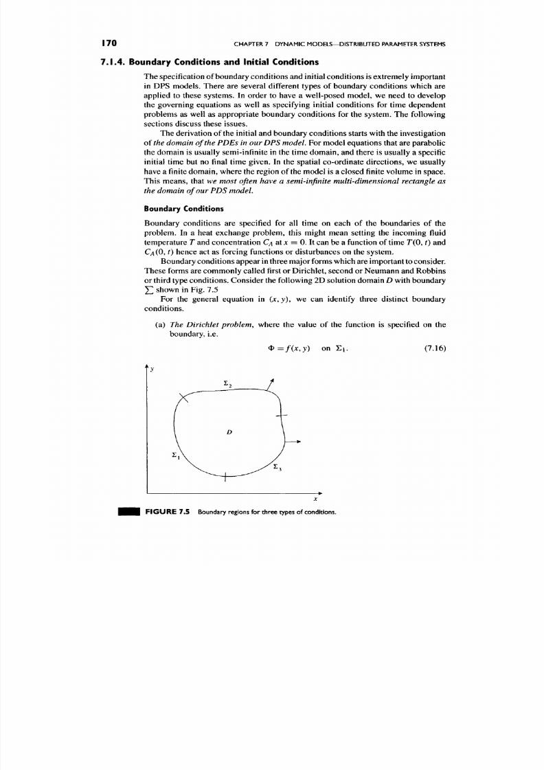
8/17/2019 Process Modelling and Model Analysis-Hangos-Cameron
http://slidepdf.com/reader/full/process-modelling-and-model-analysis-hangos-cameron 187/560
170
CHAPTER 7 DY NA MIC MODELS —DISTRIBUTE D PARAMETER SYSTEMS
7.1.4. Boundary Conditions and Initial Conditions
The specification of boundary co nditions and initial conditions is extremely imp ortant
in DPS models. There are several different types of boundary conditions which are
applied to these systems. In order to have a well-posed model, we need to develop
the governing equations as well as specifying initial conditions for time dependent
problems as well as appropriate boundary conditions for the system. The following
sections discuss these issues.
The derivation of the initial and boundary conditions starts with the investigation
of the
domain of the PDEs in our DPS
model. For m odel equations that are parabolic
the domain is usually semi-infinite in the time do main, and there is usually a specific
initial time but no final time given. In the spatial co-ordinate directions, we usually
have a finite dom ain, w here the region of the model is a closed finite volume in space.
This means, that
w e most often h ave a semi-infinite multi-dimensional rectangle as
the domain of our PDS model.
Boundary Conditions
Boundary conditions are specified for all time on each of the boundaries of the
problem. In a heat exchange problem, this might mean setting the incoming fluid
temperature
T
and concentration Q at jc = 0. It can be a function of time 7 (0 ,
t)
and
CA(0,
t)
hence act as forcing functions or disturbances on the system.
Boundary conditions appear in three major forms which are important to consider.
These forms are common ly called first or Dirichlet, second or Neumann and Robbins
or third type conditions. Con sider the following 2D solution domain D with boundary
J2
shown in Fig. 7.5
For the general equation in
( JC ,J ) ,
we can identify three distinct boundary
conditions.
(a) The Dirichlet problem, where the value of the function is specified on the
boundary, i.e.
^=f{x,y)
on E l . (7.16)
F I G U R E 7. 5 Boundary regions for three types of conditions.
8/17/2019 Process Modelling and Model Analysis-Hangos-Cameron
http://slidepdf.com/reader/full/process-modelling-and-model-analysis-hangos-cameron 188/560
DEVELOPMENT OF DPS MODELS
17 I
(b) The Neumann problem, where the n ormal derivative is specified, i.e.
-— =g(x,y)
on E2 (7,17)
an
Here d<t>/dn refers to differentiation along the normal to ^ 2 directed
away from the interior of D.
(c) The Robbins problem, third type or mixed condition, where we have
a{x,y)<^ + P{x,y)— - = y{x,y) on E3 (7.18)
an
with
a(jc,
y) > 0, P(x, y)>0 for
(JC,
y) e D. (7.19)
Assumptions Relevant to the Boundary Conditions
Conditions on the physical boundaries of the system
For a mass transfer situation, we could interpret the Dirichlet condition as setting a
concentration on the boundary,
C(0,
0 = Co. (7.20)
The Neumann condition would be equivalent to a flux at the boundary. For
example, for a perfectly isolated boundary at jc = 0 orthogonal to the
x
co-ordinate
direction the mass flux should be equal to zero, so that
^ ( 0 , 0 = 0 (7.21)
ax
for the component concentration Q .
The third type of boundary condition would be equivalent to convective mass
transfer across the boundary. If again we assume a boundary orthogonal to the
X co-ordin ate direction and assum e com ponen t mass transfer driven by the differ
ence between the concentration within the system on the boundary at
JC
= JCM with
CA(XM^ 0 and a given fixed outer concentration C* we have
^ ( X M ,
t) = K
(C* - Q(JCM, 0 ) . (7.22)
ax
Number of boundary conditions
The number of independent boundary conditions along a given co-ordinate direction
depends on the order of the partial derivative operator in that direction.
The number
of independent boundary conditions along a co-ordinate direction should be equal
to the order of the corresponding partial derivative operator Therefore, if we have
no diffusion but only convection in a direction we should specify one condition;
otherwise, with diffusion we must have two boundary conditions. The two boundary
cond itions can be on one or both sides of the interval of the co-ordinate direction. Care
needs to be taken that two or more boundary conditions are not set simultaneously
for a specified boundary region
8/17/2019 Process Modelling and Model Analysis-Hangos-Cameron
http://slidepdf.com/reader/full/process-modelling-and-model-analysis-hangos-cameron 189/560
I 72 CHAPTER 7 DYNAMIC MODELS—DISTRIBUTED PARAMETER SYSTEMS
The effect of the balance vohime shape
Note that not every bound ary of the domain in the given co-ordinate system represents
a real physical boundary. An example is a sphere where the real physical boundary
is at r = /?, /? being the radius of the sphere, but we have five virtual co-ordinate
boundaries at r = 0, ^ = 0, ^ = 27r,
(
= 0 and
(p
= 2n.
Virtual boundary conditions
express the continuity of the processes and the distributions should be constructed
accordingly in these case s. We shall see an instance of such a construction in the case
of a spherical catalyst in Example 7.2.4.
Infinitely large balance volum es
Special boundary conditions are used to express the fact that the balance volume is
very large or infinitely large in a co-ordinate direction. We may set the size of the
balance volume in that direction and
• set the concentration of the reactants to zero using Dirichlet conditions at the
boundary;
• specify that all convective and diffusive flow is zero at that boundary using
Neumann conditions.
Boundary conditions of the above types are shown in the examples given in this
chapter. The initial and boundary conditions of the packed bed plug flow catalytic
reactor are given below.
• • • EXAMPLE 7.1.4 (Derivation of the initial and boundary conditions for the
simple packed bed tubular catalytic reactor (Example 7.1.1 continued)). In order
to simplify the form of the initial and boundary conditions, we add some more
simplification assumptions.
Assumptions
additional to the ones listed as 1 -7 are:
A%. The initial distribution of component A and the initial temperature in the
reactor is uniformly constant.
A9.
The reactor is very long in the
x
co-ordinate direction to enable full
conversion.
Initial and boundary conditions
Initial conditions
Boundary conditions
Q(jc,0) = C; , r (x ,0) = r .
dx ^
dx
(7.23)
(7.24)
(7.25)
where C^'^ and 7'<') are the inlet concentration and the inlet temperature, while
C\
and r* are the initial concentrations and temperature, respectively.
Note that two boundary conditions are needed because of the presence of the
diffusion in both of the balance equations . The first condition at the outlet of the
reactor expresses the fact that the reactor is very long and the reaction is fully
com pleted before the flow exits.
8/17/2019 Process Modelling and Model Analysis-Hangos-Cameron
http://slidepdf.com/reader/full/process-modelling-and-model-analysis-hangos-cameron 190/560

8/17/2019 Process Modelling and Model Analysis-Hangos-Cameron
http://slidepdf.com/reader/full/process-modelling-and-model-analysis-hangos-cameron 191/560
8/17/2019 Process Modelling and Model Analysis-Hangos-Cameron
http://slidepdf.com/reader/full/process-modelling-and-model-analysis-hangos-cameron 192/560
EXAMPLES OF DISTRIBUTED PARAMETER MODELLING
175
DPS Model of a Double-pipe Heat Exchanger
The mathematical model of a double-pipe heat exchanger shows a lot of similarities
to the model of the tubular catalytic rector we have seen before in this chapter. The
process system consists of
a
double pipe heated from outside by condens ing saturated
steam. This situation is described by Roffel and Rijnsdorp [54]. The DPS model of
the heat exchanger is described below.
• • • EXAMPLE 7.2.1
(Double-pipe heat exchanger).
Process system
Consider
a
s imple
I D
double -p ipe exchanger where
a
l iquid stream
is
bei ng heat ed
by condensing saturated steam a t a temperat ure, Tg. This i s sh o w n in Fig . 7.6. F luid
enters a t temperature
TLC O , 0
and exits (z = L)
a t 7 L ( L ,
t) . Heat transfer takes place
between the steam
{Ts)
and the wall (rw) and then to the fluid ( 7 L ( Z , 0)- The spatial
variation is related to the fluid temperature whilst the steam temperature is
a
" lumped"
variable ,
Ts.
A ssu mp t io n s
A \
.
Th e overa ll ma ss (vol ume ) of the liquid as well as that of the wall is constant .
A2. N o diffusion take s plac e.
. 4 3 .
Steam temperature reacts instantaneously
t o
supply chan ges.
A A . Hea t transfer coefficients are cons tant .
A5.
Specific heat s and dens itie s are cons tant .
v46. Time delays are negligible fo r fluid.
Al.
Liqu id
is in
pl ug flow.
Balance vo lumes
Two volumes ( E ( ^ ^ ^ ) and E ( ^ ^ ^ ) ) for the fluid and the wall, respectively, both
of them are distributed. The rectangular co-ordinate system is chosen.
Model equations
Variables
0<z<L, 0 < r , 7 L ( Z , 0 , Tw fcO , (7.28)
where
z
is the axial co-ordinate along the tube and
L
is the tube length.
Energy balance for
the
liquid
dTL
dTL
PL^LCf-—
=
-upLAfCL-^-
+
h^ALiTy,
-
T L ) .
(7.29)
at
az
Energy balance for
the
wall
M w C w ^
=
hsAsiTs
-
Tw )
-
/iL^L(7^w
- T ^ L ) ,
(7.30)
ot
where
PL fluid density [kg/m ^]
Af flow area [m^]
CL fluid hea t cap aci ty [J /k g K]
u
fluid vel oci ty [m / s]
/ L fluid hea t tran sfer coeffi cient [ W / m ^
K ]

8/17/2019 Process Modelling and Model Analysis-Hangos-Cameron
http://slidepdf.com/reader/full/process-modelling-and-model-analysis-hangos-cameron 193/560
176 CHAPTER 7 DYNAMIC MODELS—DISTRIBUTED PARAMETER
SYSTEMS
7<"(0
Steam
7-3(0
-^TM)
z z + dz
Condensate
f
F I G U R E 7 . 6 Double-pipe heat exchanger.
. 2 ;
A L internal tube area per leng th
o f
tube [m'^ /m]
Mw mass
o f
tube per leng th [kg/ m]
Cw meta l heat capa city [J /k g K]
As
external tube area [m ^/m ]
hs
steam side heat transfer coefficient [W /m^ K]
Initial conditions
TLiz.O)=Mz). (7.31)
TAz,0)=f2{z).
(7.32)
Boundary condit ion
TL{0, t) =
T^^\t)
for all t > 0,
(7.33)
w h e re
T^^^
i s
the inlet concentrat i on
o f
the liquid.
We can
simplify
the
above PDEs
by defining som e tim e con stan ts for the syst em.
For example,
• TL = ^YT^ (char acter istic fluid heat ing tim e),
•
Tsw
=
~YT^ ( s team
to
wall thermal c onsta nt) ,
• TwL = X T ^ (^ ^ ^^ ^^^^ thermal consta nt).
Modified equations are then
^ = - « ^ + - ( ^ w -
TL) ,
(7.34)
at dz TL
^
=
—iTs
- Tw )
-
— ( r w
- T L ) .
(7.35)
dt Tsw T^wL
• • •
There are some interesting key steps
in
develo ping the DP S model above which
are
a s
follows:
1. Only one spatial co-ordinate
is
needed becaus e
o f
the plug flow as sum pti on.
2. W e
have substi tuted
t h e
consti tut ive equ ations into
t h e
balan ce equati ons.
The transfer rate relation was simply substituted as the only source term. The

8/17/2019 Process Modelling and Model Analysis-Hangos-Cameron
http://slidepdf.com/reader/full/process-modelling-and-model-analysis-hangos-cameron 194/560
EXAMPLES OF DISTRIBUTED PARAMETER MODELLING 177
200 H
r^rq
100
o-\
0 5 10
Exchanger length [metres]
F I G U R E 7. 7 Steady-state temperature profile.
potential relation U = cppT with constant physico -chem ical properties has
been substituted into the energy conservation equations (7.29) and (7.30).
3. Note that Ts is a function of time only and acts as a forcing function on the
system.
4. The model equations (7.34) and (7.35) are
coupled PDEs
since the wall
temperature (Ty^) depends on the fluid temperature
(7L).
5. A particular steady-state solution profile to the above model is shown in
Fig. 7.7.
Three-dimensional Heat Transfer
It is quite common that multi-dimensional problems arise where heat transfer is
important. Some interesting and important examples are for example:
(i) Temp erature distribution in a carcass of frozen m eat being thawed,
(ii) Temp erature profiles in walls of engine s.
(iii) Temperature profiles in high temperature reactor systems where refractory
materials are used.
The following example deals with the modelling of 3D heat transfer in a solid
body.
EXAMPLE 7.2.2 (Three-d imension al heat transfer in a solid body) .
Process system
Consider a solid body of a rectangular shape of finite length in each co-ordinate
direction. Let us assume heat generation (or loss in the solid) depending on the
spatial location.
Modelling goal
Describe the dynamic behaviour of the solid body.
Assumptions
Al.
The mass of the body and its volume are constant.
A2. The specific heat cp and the density p are constant.
A3 .
The heat generation or loss is a given function
q{x, y, z, t).
8/17/2019 Process Modelling and Model Analysis-Hangos-Cameron
http://slidepdf.com/reader/full/process-modelling-and-model-analysis-hangos-cameron 195/560
178
CHAPTER
7
DYNAMIC MODELS—DISTRIBUTED PARAMETER SYSTEMS
A4. Assum e uniform initial cond itions.
^ 5 . The temperature outside of the body is the same all over the surface and
does not change in time.
Balance volumes
A single volume en capsulating the whole solid body but this time this balance volume
is a
distributed
one.
Model equations
Variables
0<x<Lx, 0<y<Ly,
0 < z < L ^ , 0 < r,
T(x,y,zj),
(7.36)
where jc, y , z are the spatial coordinates and Lx.Ly, L^ are the lengths of the body in
the respective direction. The Cartesian co-ordinate system is selected.
Energy balance
where Kx.Ky, K^ are thermal co nductivities in the jc, y and z direc tions, respectively,
r is a function T{z, y, z, t) and c/>, p are heat capacity and density, respectively.
Initial and bound ary conditions
Initial conditions
T(x,y,z,0) = T\
(7.38)
where T* is the given uniform initial condition.
Boundary conditions
7(0,
y, z, r) -
TE,
r ( L ^ ,
y, z, t)
=
TE,
(7.39)
r(jc, 0, z, 0 = TE, r(jc,
L y,
z, 0 = TE, (7.40)
r(jc, J, 0, 0 = TE, r(jr, J, L „ 0 = TE, (7.41)
• • • where 7E is the given uniform and constant temperature of the environment.
There are again some interesting key steps in developing the above DPS model
that are worth mentioning:
1. We have substituted the potential relation U = cppT with constant physico-
chemical properties into the energy conservation equation.
2. Note that ^ is a function of time and space and acts as a forcing function on
the system.
7.2.2. Reaction Engineering
Modelling of a Pollutant in a River
As an interesting example of deriving a distributed parameter model, we consider a
modification of a problem p osed by Roffel and Rijnsdorp [54].

8/17/2019 Process Modelling and Model Analysis-Hangos-Cameron
http://slidepdf.com/reader/full/process-modelling-and-model-analysis-hangos-cameron 196/560
EXAMPLES OF DISTRIBUTED PARAMETER MO DELL ING
179
^mm EXAMPLE 7.2.3 [(Modelling of a pollutant in a river).]
Process system
Here, we are concerned about a pollutant discharged to a river and its subsequent
conc entration as it flows dow nstream. F igure 7.8 shows the geometry of the situation,
showing the cross section of the river and the representative slice over which the
conservation balanc es can be performed. N ote that the axial distance is the co-ordinate
length z.
Modelling goal
To describe the distribution of the pollutant in the river.
Assumptions
^ 1 .
The river has
a
constant cross-sectional area and the material
is
ideally
mixed over the cross section.
A2.
The pollutant disappears via a first-order reaction.
A3. Axial dispersion is present.
A4. No radial dispersion.
^ 5 . River flow is constant.
A6. The river water is considered isotherm al.
Al.
No pollution is in the river in the beginning of the process.
Balance volumes
A single distributed parameter volume encapsulating the whole river.
Model equations
Variables
0<JC <L, r >0 , c(jc,0, (7.42)
where jc is the spatial coordinate in axial direction, L the length of
the
river, t the time,
and
c
the pollutant concentration.
Component mass balance
dt
~
"az ' '^
dz^
dc dc d^c
= -u— -\-D— ^-kc,
(7.43)
Flow
area,
A
F I G U R E 7 . 8 Pollutant dispersion in a river.

8/17/2019 Process Modelling and Model Analysis-Hangos-Cameron
http://slidepdf.com/reader/full/process-modelling-and-model-analysis-hangos-cameron 197/560
I 80
CHAPTER
7
DYNAMIC MODELS—DISTRIBUTED PARAMETER SYSTEMS
with
c concen t ra tion [kg /m ^]
A flow area [m^]
u flow velocity [m/s]
D
dispersion coeffic ient [m ^/s ]
k reaction rate [s~^]
In i t ia l and boundary condit ions
c (x ,0 ) = 0 , c ( 0 , 0 - C ^ ' \ (7.44)
where Q is the inlet concentration of the pollutant.
Norm alization of the equations
We can take the governing equation and define some non-dimensional groups as
follows:
tu ^ uL ^ z ^ c ^^ kL
0 = - ; Pe=— ; Z =-; C = ~; K = —
L D L CQ u
and rearrange to get
dC dC 1 d^C
— =
+
T-KC,
(7.45)
do dz Pedz^
w h e re Pe is the Peclet number which indicates the rat io of convective to dispersive
transport . As the magnitude of P -^ oo, dispersion is negligible and we obtain plug
• I • f low behaviour. As the value of Pe -^ 0 we approach a well mixed si tuation.
The key steps in developing the DPS model above were as follows:
1. We have substi tuted the reaction rate equation as the only source into the
compon ent mass conserva t ion equa t ion .
2.
We assum ed just on e source of pollut ion at the very beginn ing of the r iver and
gave it as an initial condition. If multiple pollution sources are present then
we have to add appropriate spatial ly located addit ional source terms into the
component mass ba lance equa t ion .
Non-isothermal Reaction in a Catalyst Pellet
Finlayson [55] describes the modell ing of reactions in a spherical catalyst pelle t where
diffusion and reaction take place (jc = 0 is at the centre of the catalyst particle). The
process system is the same as in Section 3.2.2 but now we give al l of the ing redients
of i ts PDS model.
EXAMPLE 7.2.4 (Non -isotherm al reaction in a spherical catalyst pelle t) .
Process system
Consider a spherical catalyst pellet where diffusion and a first-order chemical reaction
take place.
Modelling goal
To describe the concentration profile of the reactant in the pellet.
8/17/2019 Process Modelling and Model Analysis-Hangos-Cameron
http://slidepdf.com/reader/full/process-modelling-and-model-analysis-hangos-cameron 198/560
8/17/2019 Process Modelling and Model Analysis-Hangos-Cameron
http://slidepdf.com/reader/full/process-modelling-and-model-analysis-hangos-cameron 199/560

8/17/2019 Process Modelling and Model Analysis-Hangos-Cameron
http://slidepdf.com/reader/full/process-modelling-and-model-analysis-hangos-cameron 200/560
CLASSIFICATION OF DPS MODELS I 83
The geometry of the second order multi-dimensional curve t = t(x, y, z) given in
Eq.
(7 ,54) determines the class of the PDE .
Let us illustrate how this classification is
performed by assuming that we only have a single space co-ord inate, so that Eq. (7.54)
is in the form:
t = Dx^- v^x,
(7.55)
We can then define the following special cases:
• D 7 0 gives a parabola then the original PDE is of parabolic form,
• D = 0,
Vx
^0
gives a line which we may regard as a degenerated hyperbola
giving rise to a hyperbolic PDE.
A typical exam ple of a parabolic PD E is the time dependent diffusion problem
as given in Example
7.3.1.
• • • EXAMPLE 7.3.1 (Time dependent diffusion problem). The unsteady -state prob
lem is given by
d^c d^c\
with boundary cond itions
c(x,0) = c\; c(x,l) = C2; 0 < j c < l ,
c ( 0 , j) = C 3: c ( l , j ) = C 4 ; 0<y<\,
and initial condition
c=f(x,y) atr = 0.
Hyperbolic models generally arise from vibration problems or where discontinu
ities persist in time. These can be shock w aves, across which there are d iscontinuities
in speed, pressure and density. Example 7.3.2 gives a typical example.
EXAMPLE 7.3.2 (Discon tinuities in time). On e-dimens ional wave equation
d^u 2^^^
a ? "^
a?'
where
u
is the transverse disp laceme nt at a distance
x
from on e end of a system who se
length is z.
Boundary conditions
M(0, t)
= Ml
u(z, t) =
U2 all
t.
Initial conditions
M(JC, 0) =
g(x)
at f = 0,
Generally, hyperbolic equations in two independent variables are solved numer
ically or by special techniques such as the method of characteristics.
8/17/2019 Process Modelling and Model Analysis-Hangos-Cameron
http://slidepdf.com/reader/full/process-modelling-and-model-analysis-hangos-cameron 201/560
I 84 CHAPTER 7 DYNAMIC MODELS—DISTRIBUTED PARAMETER SYSTEMS
7.3.2. The Effect of Steady-State Assumptions
The previous developm ent has lead to time varying distributed parameter models. We
can, however, modify these models through the use of steady-state conditions which
effectively eliminate the time-varying terms in the mod el.
In order to see what effect the steady-state assumption has on the form of the
DPS mo del, let us take the steady-state version of the general form of the c onservation
expression expressed in Cartesian co-ordinates as the example equation:
The associated algebraic equation reads
0 = DJC -f Dy^ + Dz^ - v^x - Vyy - v^z. (7.57)
The above equation describes an elliptic curve. In the case of two spatial variables,
we have
0= Dx^ -\- Dy^ -
VjcX
- Vyy.
(7.58)
Therefore, the steady-state assumption leads to models which are elliptic in form
and which can be solved more robustly and at less cost compared with full dynamic
mo dels. A typical example is given by the steady-state diffusion problem as given in
Example 7.3.3.
• • • EXAMPLE 7.3.3 (Steady-state diffusion problem).
_ + _ . o , o < . . ,< , ,
c(jc, 0) = ci ; c(jc, 1) = C2; 0 <
JC
< 1,
c ( 0 , y ) = C 3 ; c ( l, y) = C4; 0 < y < l ,
• • • where this is defined on a rectangular co-ordinate system.
Only a few special types of elliptic equations have been solved analytically due to
the problem of describing the boundary by equation s. In the case of difficult boundary
shapes it is essential to use an approximation method. It should be realized that the
approximation method, whether it be finite difference, finite element or method of
weighted residuals will normally provide numerical solutions as accurate as the ori
ginal model equations justify. In the real world, the modelling process and associated
data contain numerous approximations and errors.
Setting boundary conditions for such problems needs to be done with care. This
has been discussed in Section 7.1.4.
7.3.3. Assumptions Leading to the DPS Model Classes
In summary, DPS models can be of different forms dictated by the underlying
engineering assumptions as follows:
1. With
no additional assumptions they are PDE s
in
parabolic
form.
8/17/2019 Process Modelling and Model Analysis-Hangos-Cameron
http://slidepdf.com/reader/full/process-modelling-and-model-analysis-hangos-cameron 202/560
LUMPED PARAMETER MODELS FOR REPRESENTING DPSs
185
2. With a steady-state assumption they are elliptic PD Es.
3.
With
no diffusion they are first-order hyperbolic PDE s.
7.4. LUMPED PARAMETER MODELS FOR REPRESENTING DPSs
Lumping of process models of DPS is a widely used technique to transform the
set of partial differential equations in the model into a set of ordinary differential
equations. The lumped model is a finite approximation of the DPS model in the
space co-ordinate directions whereas the time variable remains the only independent
variable in a lumped mo del. Most often mod els of originally DPS systems developed
for dynamic analysis, control or diagnostic purposes are lumped in space.
The conceptual steps in lumping a DPS system model are as follows:
1.
Divide the distributed parameter balance volume of the process system into a
finite number of subvolumes.
2.
Lump each subvolume into a perfectly mixed subvolume (call it lump) with
the variables averaged.
3.
Desc ribe convection in the original DPS system as in- and outflows of the
connected set of neighbouring lumps using the appropriate direction.
4.
Describe diffusion affecting all the neighbouring lumps as in- and outflows
of neighbouring lum ps.
5.
Use the same sources for the lumps as for the original DPS mo del.
6. Develop the balance equations for every lum p.
7.
Respec t boundary cond itions at the lumps which coinc ide with the overall
boundaries of the process system.
In the case of a single spatial co-ordinate
x
the above steps reduce to:
1.
Divide the length of the process system L into a finite number of intervals
A ,
usually of equal size Ax = L/N.
2.
Lump
each subvolume into a perfectly mixed subvolume of equal size
y(k) ^ yjj^^
3. Desc ribe convection in the original DPS system as in- and outflows of the con
nected set of neighb ouring lumps using the appro priate direction, i.e. v^^^~^^
being the inflow and v<^^^^ the outflow for the
kih
lump with v being the
flowrate.
4.
Desc ribe diffusion affecting all the neighbouring lum ps, such that
D and D
Ax AJC
for the k ih lump.
Note that some of the solution methods do a kind of lumping when solving PDE
models, e.g. the method of lines (see details in Chapter 8).
As an illustration of the above procedure, a lumped model of the double-pipe
heat exchanger described in Example 7.2.1 is given.
8/17/2019 Process Modelling and Model Analysis-Hangos-Cameron
http://slidepdf.com/reader/full/process-modelling-and-model-analysis-hangos-cameron 203/560
8/17/2019 Process Modelling and Model Analysis-Hangos-Cameron
http://slidepdf.com/reader/full/process-modelling-and-model-analysis-hangos-cameron 204/560
APPLICATION EXERCISES
187
variation in key states as a function of spatial position. In many cases, we simplify
our approach by adopting a lumped parameter view of the system. This can be most
useful but there are clearly occasion s when that assum ption is not valid. In those cases
we are forced to model the spatial variations.
In modelling proc ess systems as DPS m odels, the level of complexity rises
signif
icantly. This has im plications on the solution techn iques as w ell as for
the
development
of the model. Only when the lumped parameter system assumption is invalid, should
we consider the need to treat the problem as a distributed system. Chapter 8 deals
with a variety of techniques for solving the distributed parameter models.
7.6. REVIEW QUESTIONS
Q7.1,
Desc ribe why distributed parameter models arise in process engineering
applications. (Sections 7.1 and 7.2)
Q7.2.
W hat are the principal geometries used in the developm ent of distributed
parameter models? Give a process engineering example of each approach describing
how it arises. (Section 7.1)
Q7.3.
W hat are the roles of initial cond itions and boundary co nditions in the formula
tion of distributed parameter models? Describe the three principal types of boundary
conditions and give some examples of their use in practical modelling problems.
(Section 7.1)
Q7.4. W hat are the advantages and disadvantages of non-dim ensional forms of the
governing PDE s? (Section
7.1.5)
Q7,5. Describe the classes of mod elling assumptions which affect the form of the
DPS model equations. Give examples illustrating the possible effects. (Section 7.1)
Q7.6.
Describe the three main forms of partial differential sy stems which arise
from distributed parameter modelling. What are the most common forms in process
engineering? (Section 7.3)
Q7.7. Describe the process of representing the behaviour of partial differential equa
tion models in terms of lumped parameter m odels. Wh at are the key characteristics of
the resultant equation systems in terms of problem size and accuracy? (Section 7.4)
7.7. APPLICATION EXERCISES
A7.1. Develop the general mass and energy balance equations for a tubular plug flow
reactor, where the reaction kinetics are given by the following general expression:
Assu me that the inlet flowrate is F/,2, inlet concentration is CAJH and temperature TQ.
The reactor will be cooled or heated depending on whether the reaction is exothermic
or endothermic.
Give the initial conditions and boundary conditions for such a system.
A7.2.
For the application example in A7.1 develop a lumped model representation
for the general problem.
8/17/2019 Process Modelling and Model Analysis-Hangos-Cameron
http://slidepdf.com/reader/full/process-modelling-and-model-analysis-hangos-cameron 205/560
188 CHAPTER 7 DYN AMIC MODELS—DISTRIBUTED PARAMETER SYSTEMS
A7.3, Consider the modelling of a liquid-liq uid co ntactor or extraction column where
a solute A contained in a liquid B is extracted using a solvent S in countercurrent flow.
Assume that the liquid rates are
LB
and
Ls
and that a simple mass transfer relation
holds for the transfer of solute from B to 5.
Show the fundamental geometry to be used in developing the balance equations .
A7.4. Consider the development of a dynam ic model to predict the behaviour of a
packed bed adsorber. In this case, a gas stream contains a hydrocarbon which must
be adsorbed onto an activated carbon adsorbent. Assume that the bulk concentration
of the species is Q and that the adsorbed concentration is C^. The relationship which
relates
Ca
to Q is given by
Ca =f(Cb)'
Assume that the bed voidage is e , the bed cross-sectional area is A and that the
interpellet gas velocity is
u .
Develop the dynamic mass balance w hich describes the
behaviour of the adsorbed species with time and length along the adsorber.
Define appropriate initial and boundary conditions for such a situation.
A7.5. Consider a well-mixed batch reactor for the production of octyl phthalate in
which an endothermic reaction takes place between octanol and phthalic anhydride.
The temperature profile of the batch is controlled by the use of a circulating hot oil
system which consists of a h eat transfer coil located inside the reactor and an external
gas fired heater which m aintains a fixed inlet temperature of oil to the reactor.
Mo del the temperature profile in the hot-oil coil within the reactor and use it to
predict the dynamics of the energy transfer to the batch. Clearly state all assumptions
in the model.
A7.6. A hot rectangular slab of steel is hardened by immersing it vertically in a
tank of oil using an overhead crane . Develop a dynamic model of the system, stating
clearly the assumptions used in developing the model.
A7.7. Consider the problem of freezing of a lake due to subzero air temperatures
during winter. Develop a one dimensional model of the temperature as a function of
time and depth in the lake as the freezing occu rs. Consider how the ice layer on top of
the cold water increases in thickness as the process proceeds. State the assumptions
used in developing the model as well as the necessary boundary and initial con ditions
needed for the so lution.
Consider how the moving ice-water interface can be tracked as time proceeds.
A7.8. Consider the problem of the double pipe heat exchanger given in Exam ple
7.2.1.
Derive the governing energy balance equations using the microscopic balance
approach as set out in section
7.1.3.
Com pare the final derived balance equations w ith
those in the example.
A7.9. For the 3D heat transfer problem in a rectangular slab given in Example 7.2.2,
derive the governing energy balance equation from the application of a microscopic
balance. Compare your model with that shown in the example.
A7.10,
Derive, using the microscopic balance approach, the model described in
Example 7.2.3 which considers the concentration changes in time for flow of a
pollutant in a river. Check your d evelopment against that stated in the exam ple.
A7.11.
For the double-pipe heat exchanger problem given in Exam ple
7.2.1,
consider
the case where the outer tube side is now a counter-current liquid process stream which
provides heating to the colder inner tube stream. Derive the distributed parameter

8/17/2019 Process Modelling and Model Analysis-Hangos-Cameron
http://slidepdf.com/reader/full/process-modelling-and-model-analysis-hangos-cameron 206/560
APPLICATION EXERCISES
189
model which describes the temperature dynamics for both the hot stream, the cold
stream and the tube wall.
A7.12. Derive the mass and energy balance equations related to the mass and heat
transfer in a spherical catalyst pellet given in Example 7.2.4. Use a microscopic
balance approach to do this and compare your model with the governing equations
given in the example.

8/17/2019 Process Modelling and Model Analysis-Hangos-Cameron
http://slidepdf.com/reader/full/process-modelling-and-model-analysis-hangos-cameron 207/560
This Page Intentionally Left Blank
8/17/2019 Process Modelling and Model Analysis-Hangos-Cameron
http://slidepdf.com/reader/full/process-modelling-and-model-analysis-hangos-cameron 208/560
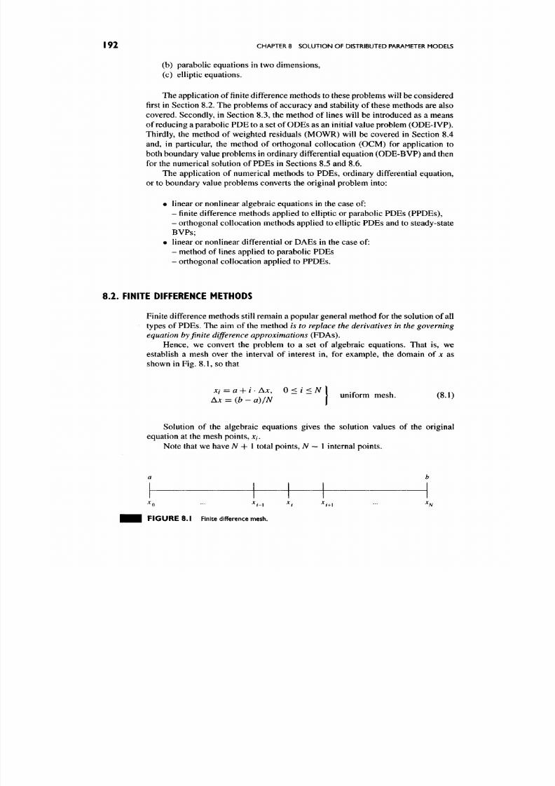
8/17/2019 Process Modelling and Model Analysis-Hangos-Cameron
http://slidepdf.com/reader/full/process-modelling-and-model-analysis-hangos-cameron 209/560
I 92 CHAPTER 8 SOLUTION OF DISTRIBUTED PARAMETER MODELS
(b) parabolic equations in two dimensions,
(c) elliptic equations.
The application of finite difference method s to these problems will be cons idered
first in Section 8,2. The problems of accuracy and stability of these methods are also
covered. Secondly, in Section 8.3, the method of lines will be introduced as a means
of reducing a parabolic PDE to a set of OD Es as an initial value problem (OD E-IVP ).
Thirdly, the method of weighted residuals (MOWR) will be covered in Section 8.4
and, in particular, the method of orthogonal collocation (OCM) for application to
both boundary value problem s in ordinary differential equ ation (OD E-BV P) and then
for the numerical solution of PDEs in Sections 8.5 and 8.6.
The application of numerical methods to PDEs, ordinary differential equation,
or to boundary value problems converts the original problem into:
• linear or nonlinear algebraic equations in the case of:
- finite difference methods applied to elliptic or parabolic PDEs (PPDEs),
- orthogonal collocation metho ds applied to elliptic PDEs and to steady-state
BVPs;
• linear or nonlinear differential o r DA Es in the case of:
- method of lines applied to parabolic PDEs
- orthogonal collocation applied to PPDEs.
8.2. FINITE DIFFERENCE METHODS
Finite difference method s still remain a pop ular general method for the solution of all
types of PDEs. The aim of the method
is to replace the derivatives in the governing
equation by finite difference approximations (PDAs).
Hence, we convert the problem to a set of algebraic equations. That is, we
establish a mesh over the interval of interest in, for example, the domain of jc as
shown in Fig. 8.1, so that
. " " ' ^ " . . " ^ ' • ? / ; . ^ - ' - ^ } uniform m esh. (8.1)
Ax = {b
—
a) IN
•
Solution of the algebraic equations gives the solution values of the original
equation at the mesh p oints, jc/.
Note that we have
N
+ 1 total po ints,
A
— 1 internal points.
F I G U R E 8.1 Finite difference mesh.

8/17/2019 Process Modelling and Model Analysis-Hangos-Cameron
http://slidepdf.com/reader/full/process-modelling-and-model-analysis-hangos-cameron 210/560
FINITE DIFFERENCE METHODS
I 93
8.2.1.
Finite Difference Approximations
Consider a continuous function u(x), where we w rite a Taylor series expansion about
Xj
so that
uixi + Ax) = u(xi) + Axu(xi) + ^Ax^u'\xi) + ^ A X^M'"(JC/) + • • • , (8.2)
u(xi - Ax) = u(xi) - Axu{xi) +
^
Ax^M^'te) - ^Ax^u''\xi) + • • • . (8.3)
From these expansions or combinations of them we can obtain the following PDAs.
Using the notation «/
=
u(xi), we have the following first- and second -order
approximations, formed using forward, backward or central differences.
First-order approximations:
^ Mxi)^ ^
Ui+i
-
Ui
^ ^^ ^^ ^ (forward difference), (8.4)
ox Ax
. ^ du^ ^ Ui-Ui-i ^ ^^^^^ (bac kward difference). (8.5)
ax Ax
Second-order approxim ations:
^ duOci)_
^ Ui^i-ui.i
^ ^ ^ ^ ^ 2 )
( ^ ^ 1
difference), (8.6)
ox lAx
n
d M (X ,) MI_I_I — 2M / + M/_l o
< = — ^ - - ^ '^ ' ^ + 0 ( A J C 2 ) (central difference). (8.7)
It is obvious that higher order derivatives can be estimated as well as FDAs of
higher accuracy. These FDA s form the basis of the finite difference method . D etailed
coverage of finite difference methods is given by Smith [56 ].
8.2.2. Parabolic Equations in One Dimension
These are evolutionary problems since they are not only dependent on a spacial
variable x but are transient. H ence, the so lution is a function of jc and t,
• • • EXAMPLE 8.2.1 We consider an explicit method for the problem of unsteady
diffusion in one dimension,
with boundary conditions
u(0,t)=
1, w (l ,0 = 0
and initial conditions
u{x,0) = 2x:
0 < jc < 2 a n d 2 ( l - j c ) : ^ < J C < 1 ,
where we assume
k
=
constant.
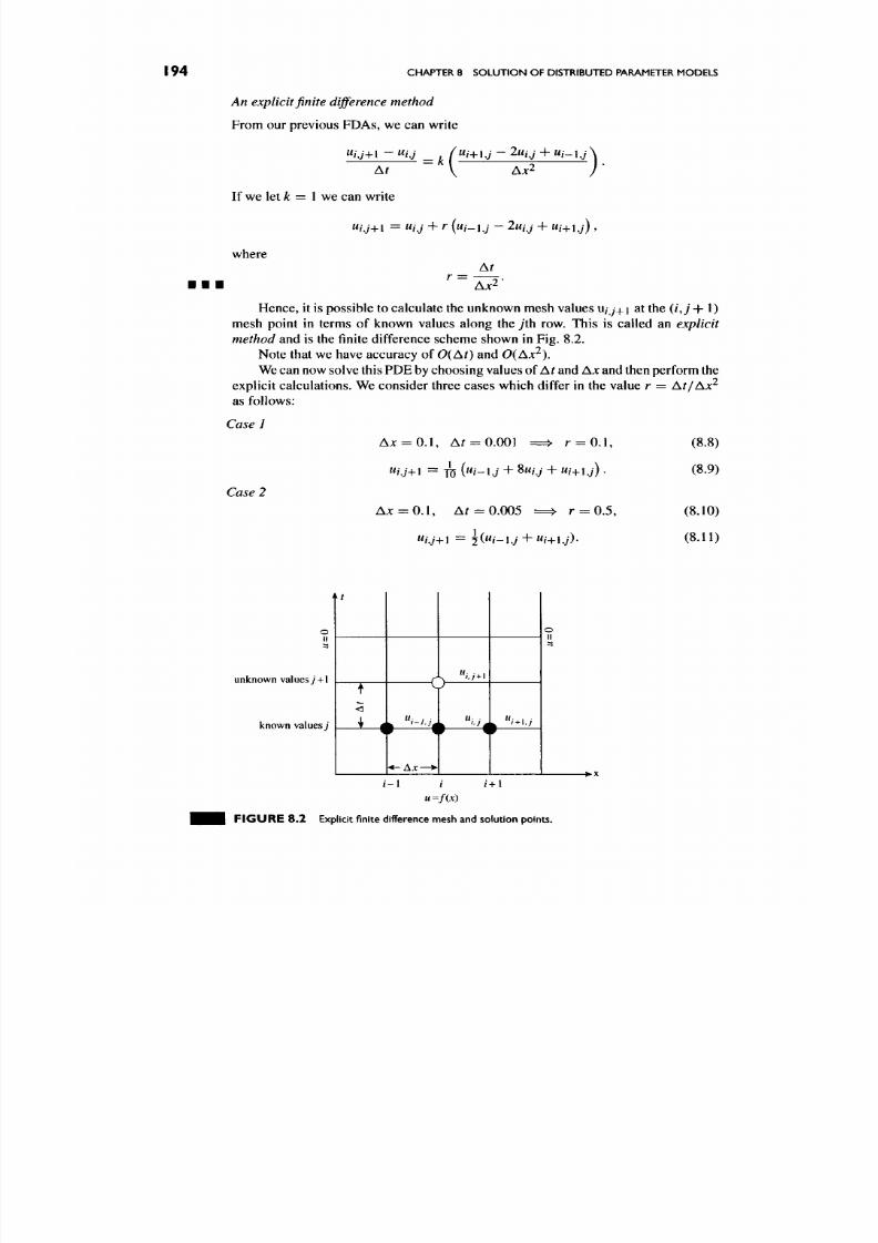
8/17/2019 Process Modelling and Model Analysis-Hangos-Cameron
http://slidepdf.com/reader/full/process-modelling-and-model-analysis-hangos-cameron 211/560
194
CHAPTER 8 SO LUT ION OF DISTRIBUTED PARAMETER MODELS
An explicit finite difference method
From our previous PDAs, we can write
"/•J+l
^
= k(^
) •
t V AJC2
If we let /: = 1 we can write
where
At
Hen ce, it is possible to calculate the unknown mesh values u/y^_i at the
(ij + 1)
mesh point
in
terms
of
known values along the yth row. This
is
called
an
explicit
method and is the finite difference scheme shown in Fig.
8.2.
Note that we have accuracy of 0{At) and 0(AJC^).
We can now solve this PDE by choosing values of Ar and
Ax
and then perform the
explicit calculations. We consider three cases w hich differ in the value r =
At/Ax^
as follows:
Case
1
Case
2
AJC = 0 . 1 ,
Ar =
0.001
= r =
0.1,
AJC
= 0 . 1 , Ar = 0.005
r
= 0.5,
" / j+l =
l(^i-ij
+ «/+l,;)-
(8.8)
(8.9)
(8.10)
(8.11)
unknown values j+1
known
values;
4r
^
1
1
^
< - A J C — •
s w>i
J
,. / ^ i . ;
P
o
II
• x
/-I / i+l
ii=f(x)
F I G U R E 8.2 Explicit finite difference mesh and solution points.
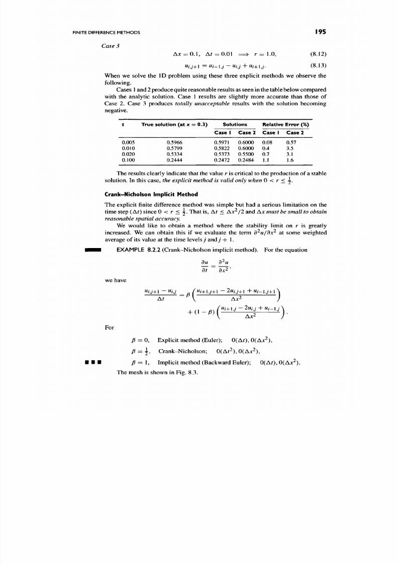
8/17/2019 Process Modelling and Model Analysis-Hangos-Cameron
http://slidepdf.com/reader/full/process-modelling-and-model-analysis-hangos-cameron 212/560

8/17/2019 Process Modelling and Model Analysis-Hangos-Cameron
http://slidepdf.com/reader/full/process-modelling-and-model-analysis-hangos-cameron 213/560
196
CHAPTER 8 SOLUTION OF DISTRIBUTED PARAMETER MODELS
y+1
7 = 0
^ ^ ^ - 1 , ; > 1 A
"i,j+\
A ^^-H.j+l
unknown values of u
known values of u
/ =0 / - I / + 1
F I G U R E 8 . 3 Crank-Nicholson finite difference scheme.
0.25 0.5
F I G U R E 8 . 4 Stability regions for the Crank-Nicholson method.
The Stability of these equations is given by
At 0.5
AJC2
- l - i p '
(8.14)
We can plot r versus
p
to obtain the stability prop erties of the FDA for
du/dt
=
d^u/dx^. This is shown in Fig. 8.4.
Solution of the equations
The solution of the Crank-Nicholson method as well as the fully implicit method
means that it is necessary to solve a tridiagonal system of equations to find the
unknowns.
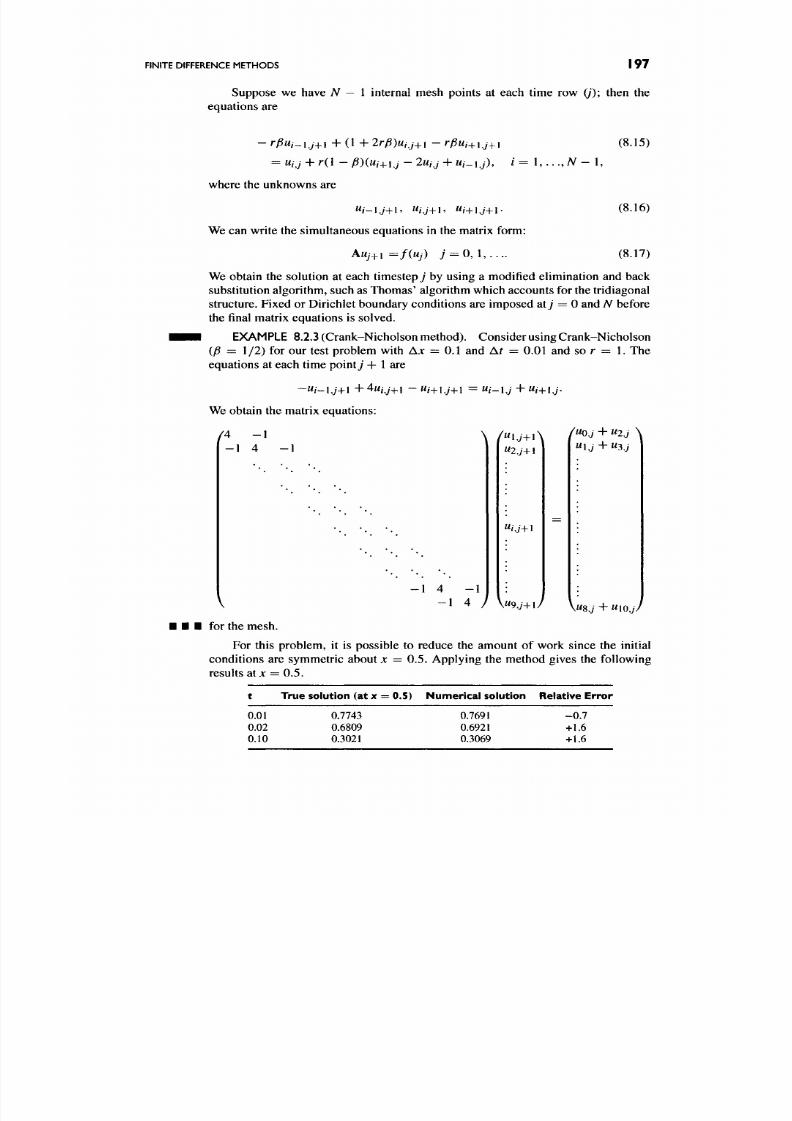
8/17/2019 Process Modelling and Model Analysis-Hangos-Cameron
http://slidepdf.com/reader/full/process-modelling-and-model-analysis-hangos-cameron 214/560
FINITE DIFFERENCE METHODS
197
Suppose we have N — I internal mesh points at each time row (/); then the
equations are
-
rpuj-ij^i +
(1
+
2rP)uij^i
- rpui^ij^i
(8.15)
= w/j + r ( l - p){ui^[j - 2uij + M /_ij), / = 1 , . . . , A^ - 1,
where the unknowns are
« /-l,7+l» W/j+i, M/+1J+1. (8.16)
We can write the simultaneous equations in the matrix form:
Auj^l=f{uj) 7 = 0,1,.... (8.17)
We obtain the solution at each timestepy by using a modified elimination and back
substitution algorithm, such as Thomas' algorithm which accounts for the tridiagonal
structure. Fixed or Dirichlet boundary conditions are imposed aij = 0 and A ^ before
the final matrix equations is solved.
EXAMPLE 8.2.3 (Crank-Nicholson method). Consider using Crank-N icholson
(P = 1/2) for our test problem with A JC = 0.1 and At = 0.01 and so r = 1. The
equations at each time point j + 1 are
We obtain the matrix equations:
/ 4
- 1
- 1 4 - 1
\
W/j+ l
- 1 4 -1
- 1 4 / VM9J+I/
"2,7+1
\W8,y + M l O j /
for the mesh.
For this problem, it is possible to reduce the amount of work since the initial
conditions are symmetric about x = 0.5. Applying the method gives the following
results at jc = 0.5.
t Tru e solution (at
x =
0.5) Nu me rical solution Relative Error
0.01
0.0 2
0.10
0.7743
0.6809
0.3021
0.7691
0.6921
0.3069
- 0 . 7
+1.6
+1.6

8/17/2019 Process Modelling and Model Analysis-Hangos-Cameron
http://slidepdf.com/reader/full/process-modelling-and-model-analysis-hangos-cameron 215/560
198
C H A P T E R
8
S O L U T I O N
OF
D I S T R I B U T E D P A R A M E T E R M O D E L S
This shows app roximately the same error as the explicit method (but this method
uses
10
times
the
number
of
steps).
The
results show
the
increased accuracy
of
Crank-Nicholson O(A r^) over the Euler method 0(At) and the ability of the Crank-
Nicholson method to take large steps
in At.
8.2.3. Parabolic Equations
in
Two Dimensions
Here, we are concerned about the solution
of
the equation
a7~ ya^^a^j
(8.18)
over the rectangular region 0 < x < a, 0 < y < b, where u is initially known at all
points w ithin and on the boundary of
the
rectangle, and is known subsequently on the
boundary for all time. That is, we have initial conditions for the w hole region as w ell
as boundary conditions. The mesh
is
shown
in
Fig. 8.5.
We define the co-o rdinates of the mesh as (jc, j , t) with
Xi
= iAx;
yj=jAy; tn
= nAt, (8.19)
where ij, n are positive integers and w e denote the value of u at the m esh points as
u(iAxJAy,
nAt) =
M/J,,J. (8.20)
The simplest finite difference method would be an explicit method. Let us
consider this approach to our problem, as well as some others.
b
M-\
J
3
2
1
0
- * -
- * -
- ^
- ^
0
1 2 3 / A^-1 fl JC
F I G U R E 8.5 Finite difference mesh for 2D parabolic equations.
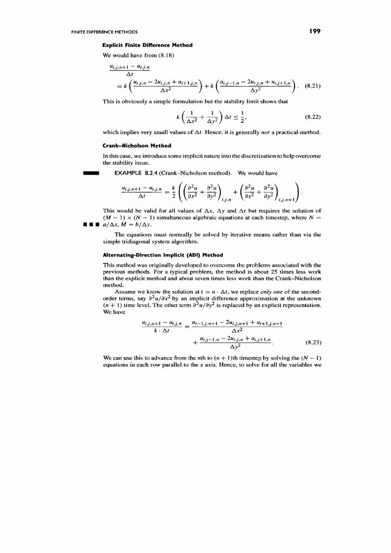
8/17/2019 Process Modelling and Model Analysis-Hangos-Cameron
http://slidepdf.com/reader/full/process-modelling-and-model-analysis-hangos-cameron 216/560
FINITE DIFFERENCE METHODS I 99
Explicit Finite Difference Method
We would have from (8.18)
^iJ,n+\ ~~ ^ij,n
This is obviously a simp le formulation but the stability limit show s that
which implies very small values of At. Hen ce, it is generally not a practical method.
Crank-Nicholson Method
In this case, we introduce some im plicit nature into the discretization to help overcome
the stability issue.
^ • B EXAMPLE 8.2.4 (Crank-N icholson method). We would have
At
_ _ , . . ,
This would be valid for all values of
AJC, Ay
and
At
but requires the solution of
( M — l ) x ( A ^ — 1 ) simultaneous algebraic equations at each timestep, where N =
a/Ax, M
=
b/Ay.
The equations must normally be solved by iterative means rather than via the
simple tridiagonal system algorithm.
Alternating-Direction Implicit (ADI) Method
This method was originally developed to overcome the problems associated with the
previous methods. For a typical problem, the method is about 25 times less work
than the explicit method and about seven times less work than the Crank-Nicholson
method.
Assum e we know the solution at f = n
•
A ^ we replace only one of the second-
order terms, say
d^u/dx^
by an implicit difference approximation at the unknown
(n
4- 1) time level. The other term
d^u/dy^
is replaced by an explicit representation.
We have
k' At ~ Ax^
Ay'^
We can use this to advance from the nth to (n + l)th timestep by solving the (N
—
\)
equations in each row parallel to the
x
axis. Hence, to solve for all the variables we
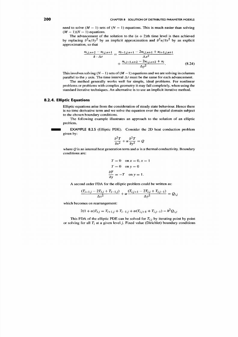
8/17/2019 Process Modelling and Model Analysis-Hangos-Cameron
http://slidepdf.com/reader/full/process-modelling-and-model-analysis-hangos-cameron 217/560
200 CHAPTER
8
SOLUT ION OF DISTRIBUTED PARAMETER MODELS
need to solve (M - 1) sets of (N - 1) equations. This is much easier than solving
(M
-
1){N
- 1) equ ations.
The advancement of the solution to the (n + 2)th time level is then achieved
by replacing
d^u/dy^
by an implicit approximation and
d^ii/dx^
by an explicit
approximation,
so
that
This involves solving (A — 1) sets of (M — 1) equa tions and we are solving in colum ns
parallel to the y axis. The time interval Ar must be the same for each advancement.
The method generally works well
for
simple, ideal problems.
For
nonlinear
problems or problems with complex geometry
it
may fail completely, when using
the
standard iterative techniques. An alternative is to use an implicit iterative m ethod.
8.2.4. Elliptic Equations
Elliptic equations arise from the consideration of steady state behaviour. Henc e there
is no time derivative term and we solve the equation over the spatial domain subject
to the chosen boundary conditions.
The following example illustrates an approach to the solution of an elliptic
problem.
• • • EXAMPLE
8.2.5
(Elliptic
PDE).
Consider
the 2D
heat conduction problem
given by:
where
Q
is an internal heat generation term and o? is a thermal conductivity. B oundary
conditions are:
T = 0 onjc = 0, j c = l
r = 0 on J = 0
— = — T on y = 1.
dy
A second order FDA for the elliptic problem could be written as:
{Ti^Uj-2Tij^Ti.ij) , (Tij^i-lTjj^Tjj.i)
^
I ? K? - ' "
which becomes on rearrangement:
2(1
+
a)Tij
=
Ti^ij
+
Ti^xj
+
a(Tij^i
+
r / j_ i )
-
h^Qtj,
This FDA
of
the elliptic PDE
can be
solved
for Tij by
iterating point
by
point
or solving for all 7/ at a given level j . Fixed value (Dirichlet) boundary conditions
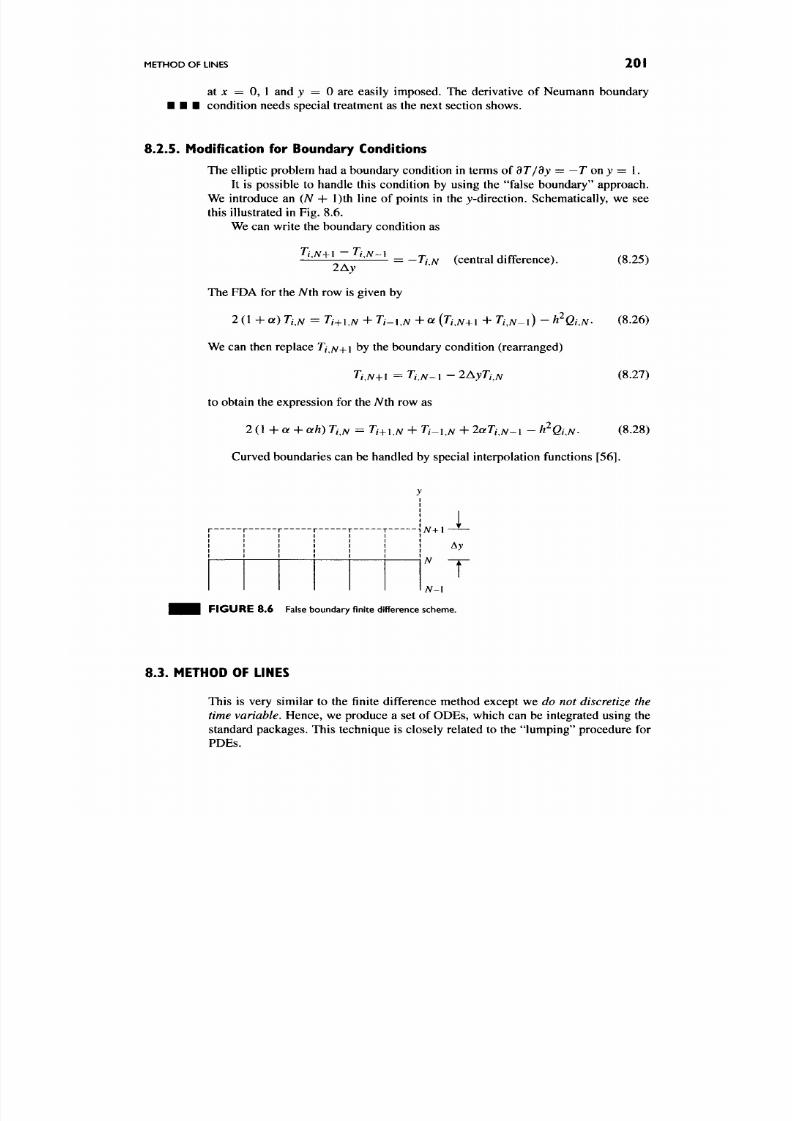
8/17/2019 Process Modelling and Model Analysis-Hangos-Cameron
http://slidepdf.com/reader/full/process-modelling-and-model-analysis-hangos-cameron 218/560
METHOD
OF
LINES 201
at jc
= 0, 1 and
>'
= 0 are
easily imposed.
The
derivative
of
Neumann boundary
condition needs special treatment as the next section shows.
8.2.5. Modification for Boundary Conditions
The elliptic problem
had a
boundary condition
in
terms
of dT/dy = — T
on
j = 1.
It
is
possible
to
handle this condition
by
using
the
"false boundary" approach.
We introduce an (A^ + l)th line of points in the j-dire ctio n. Schematically, we see
this illustrated
in
Fig.
8.6.
We can write the boundary condition as
2Ay
- Ti^N (central difference).
(8.25)
The FDA
for
the A^th
row is
given
by
2 (1 -f a) nN = Ti+iN + Ti^iN + cc {Ti^N+i + Ti^N-\) -
h^QlM'
(8.26)
We can then rep lace 7"/ //_j_i by the boundary condition (rearranged)
Ti^N-\-\ = Ti^N-\ - 2AyTi^N
(8.27)
to obtain
the
expression
for the
A th
row as
2{l-^a^ah)
Ti^N
=
Ti^hN
+
7 /-l,A^
+
2aTi^N-l
- h^Qi,N-
(8.28)
Curved boundaries can be handled by special interpolation functions [56].
- ,
^ ^ 1
A ^ + l
A
Ay
T
N-\
F I G U R E
8.6
False bou nda ry finite difference scheme .
8.3. METHOD
OF
LINES
This is very similar to the finite difference method except we do not discretize the
time variable.
Hence,
we
produce
a set of
ODEs, which
can be
integrated using
the
standard packages. This technique is closely related to the "lumping" procedure for
PDEs.

8/17/2019 Process Modelling and Model Analysis-Hangos-Cameron
http://slidepdf.com/reader/full/process-modelling-and-model-analysis-hangos-cameron 219/560
202 CHAPTER 8 SOLUTION OF DISTRIBUTED PARAMETER MODELS
Thus, we convert the equation
du d^u
to
^=fi{u),
i =
0,..„N. (8.30)
at
W K K M
EXAMPLE 8.3.1 (Packed bed reactor with radial disper sion). Consid er a packed
bed reactor with radial dispersion:
S=as/^c-\-pR(c),
at
dc dc
— = 0 atr = 0; — = B /w (c ( l ,z ) - CwCO) •
dr or
We have, after expanding v ^ c the discretized equations:
Ac.
At
L ^ ^ V n / 2Ar J
where a = 1, 2, 3 depen ding on geome try.
For the derivative boundary conditions we use a false boundary to give
— TT = 0 ; — =
fi«w
(CA - Cw )
2 A r 2 A r
and the equations for / = 0 and A are found from substituting the boundary cond itions
into the governing equations.
Thus, we have a set of ODEs
den
la ^
. ^ „
dr AH
dCj
"dr
dCA^
dr L ^ ^ \
n /
2A r J
— = Of — 2
{a -
l)B«w(cw -CN)\+
PRN-
A common problem with the method of lines is that the resulting set is often stiff
and thus implicit OD E m ethods are normally needed to solv e these problem s.
EXAMPLE 8.3.2 (A dispersio n-conv ection problem). Consider a disp ersio n-
convection problem given by
dy
_
d^y dy
c = constant > 0.

8/17/2019 Process Modelling and Model Analysis-Hangos-Cameron
http://slidepdf.com/reader/full/process-modelling-and-model-analysis-hangos-cameron 220/560
METHOD OF WEIGHTED RESIDUALS 203
Boundary conditions and initial condition are
>; (0 ,0 = 1, ^ > 0 ,
dy
/ ( 1 , 0 = 0, ^ > 0 ,
ax
j(jc ,0 ) = 0, 0 < j c < l .
Applying the method of lines gives
dt
(1/A^)2
• • • yi(0) = 0, / = , . . .,N, yo(t) = 1, yNuiO = W - l ( 0 -
In this case, the stiffness of the problem is proportional to the square of the
discretization value
A .
8.4. METHOD OF WEIGHTED RESIDUALS
In this section, we cons ider the numerical solution of general boundary value problems
(ODE-BVP) as a prelude to the solution of PDEs in Section 8.6. The key concept is
that we substitute a trial function, typically a power series function into the governing
equation which creates a "residual" or error since the chosen function is rarely the
correct solution. We then minimize the "weighted residual" by applying various
weighting c riteria which distribute the error in different ways over the spatial dom ain.
Hence, the term method of w eighted residuals (MOW R). A comprehensive treatment
of these techniques in chemical engineering is given by Finlayson [55,57].
• • • EXAMPLE 8.4.1 (A simple heat conduction problem). Consider a simple heat
conduction problem which we will use as a test problem [57]. Here, we have the
BVP:
d / dM\
— I C(M)-— J = 0 where c{u) =
1
-h
aM
dx \ dxj
with boundary c onditions
M(0) = 0; M(1) =
1.
The exact solution is given by:
u(x) = - 1 + V 3 J C + 1 for a = 1,
M(0.5)
=0.5811
• • I We will now develop and com pare MO WR approach es with the analytical solution.
8.4.1. Basic Steps in the Method of Weighted Residuals
The procedure for applying the MOWR is as follows:
Step 1.
Choose a trial function and expand the function.
Step
2. Try and fit boundary conditions to the trial function.

8/17/2019 Process Modelling and Model Analysis-Hangos-Cameron
http://slidepdf.com/reader/full/process-modelling-and-model-analysis-hangos-cameron 221/560
204 CHAPTER 8
SOLU TION OF DISTRIBUTED
PARAMETER MODELS
Step
3. Substitute the trial function into the problem and form a residual.
Step
4.
Make the residual zero by using one of the following criteria:
Collocation, Galerkin, Least squares, Subdomain or Moments.
These criteria distribute the error in the solution in different ways and can be
used for a variety of applications.
• • • EXAMPLE 8.4.2 (MOWR approach to the simple heat conduction problem).
We can now apply the MOWR approach to our simple heat conduction problem.
Step 1: Choose 0// = Zl/L^ ^i^^ ^^ the trial function (or test solution).
Step 2: Now fit the boundary con ditions to the trial function:
0;y (O) = 0 implies tha t CQ = 0,
0;y(l) = 1 implies that y ^ Q = 1
/ =1
or
N
/ =1
or
7V+1
ci = 1 - ^ c/
SO
that we can modify and write the trial function as
/ N+1 \ N+1
\ i=l I i=2
07V = ^ + ^ Q
(x^ - x)
.
Finally, we have
N
( l>N=x-hJ^Ai(x^^^-x).
which we will now use as our approximate so lution. Notice that we have the unknown
coefficients A/. The higher the order of the polynomial the more A/ terms we have.
It should be noted that regardless of the values of Aj the boundary conditions are
satisfied by the trial function. Put the values of jc = 0 and jc = 1 in and s ee.
Step 3:
Form the residual by substituting the trial function into the expanded
BVP to obtain
R(x, 07V)
= (1 +
a(l)N)(l>N
+ a (0 ;^ )^
where 0j^ and 0jl^ are the first and second derivations of </>//.
8/17/2019 Process Modelling and Model Analysis-Hangos-Cameron
http://slidepdf.com/reader/full/process-modelling-and-model-analysis-hangos-cameron 222/560
METHOD OF WEIGHTED RESIDUALS 205
Then, the weighted residual is
1
WkR (x,(l)M)dx = 0, k = I,.. .,N.
0
1
Step 4: App ly a weighting criterion to reduce the residual to zero. That is,
we choose a method of distributing the error in a particular way. We consider
• • • a collocation approach in this case, although other approac hes can be used.
Collocation method
Here, we force
0A^
to satisfy the residual at a given set of
A
points. This leads to
N
algebraic equations whose solution gives the value of the coefficients A/. At the
collocation points, the residual R{x, 0A^) = 0. As more collocation points are used,
we force the approximation to become more accurate.
Hence, for the collocation method, the weight (w^) is
W]^ = 8{x
— Xk) (dirac delta), (8.31)
meaning that
w^ = I
when
x = x^,
otherwise
Wk =
0.
Hence,
1
I WkR(x,
<t>N)
dx = R{xk,
(PN)
=
0. (8.32)
0
• • • EXAMPLE 8.4.3 (A fixed point collocation examp le). Collocate at jc = 0.5 .
Here we want the residual to be zero at the mid-point.
From the trial function <>A we obtain
01 =jc + Ai(x^ -j c ) , 01 = 1 +y 4i (2 jc - 1), 0 ' / = 2Ai.
The residual becom es
/ ?( jc ,0 i) = [ l + Q f [ x + A i ( j c 2 - j c ) ] ] 2 A i + o f [ l + A i ( 2 j c - l ) ] ^
Now let JC = J (collocation point),
o?
=
1
giving the residual equation
[l + ^ + Ai ( I - ^ ) ] 2Ai +
1
+ A i d - 1) = 0,
-^Aj
-f- 3Ai + 1 = 0, Ai = -0 .3 1 6 6 .
The other root is not feasible, so the approximate solution is
0 1 = j c - 0 . 3 1 6 6 ( j c ^ - x ) .
and
01(0.5) = 0.5795
• • • which com pares well with the analytic solution 0.5 81 1.
8/17/2019 Process Modelling and Model Analysis-Hangos-Cameron
http://slidepdf.com/reader/full/process-modelling-and-model-analysis-hangos-cameron 223/560
206 CHAPTER 8 SOLUTIO N OF DISTRIBUTED PARAMETER MODELS
8.5. ORTHOGONAL COLLOCATION
In this case, the choice of collocation points is not arbitrary. The trial functions are
chosen as sets of orthogonal polynomials and the collocation points are the roots
of these polynomials. Also, we can formulate the solution so that the dependent
variables are the solution values at the collocation points, rather than the coefficients
of the expansion [57]. The use of orthogonal polynomials means that the solution
error decreases faster as the polynomial order increases in comparison to arbitrarily
placed collocation points.
Instead of any trial functions, <pi(x), let us use orthogonal polynomials of the
form
m
Pm(x) = J2cix\ (8.33)
We can define the polyn omials by
b
f
a
wix)Pnix)Pfn{x)
djc = 0, M = 0, 1 ,. . ., m - 1. (8.34)
A particular sequence of orthogonal polynomials leads to the
Legendre
polynomials'.
Po = l , P i ^ j c , P 2 =
1 - 3 J C ^
. . . (8.35)
with the polynomial Pm(x) having m roots, which become the collocation points.
Other orthogonal polynomials such
as
the Jacobi polynomials can also
be
used
[58].
In
the next two sections, w e obtain the key polynomial expansions suitable for prob lems
with symmetry and those without symmetry.
8.5 .1 .
Orthogonal Collocation with Symmetry
Consider problems on the domain 0 < jc < 1 and symmetric about x = 0. These
can typically be reactor or catalyst problems. We can exploit the geometry of the
problem by considering polynomials expanded in powers of jc [57]. For problems
with Dirichlet boundary conditions, we could use
N
yix)=y{l) + {l
- x 2 ) ^ a / P / _ i ( j c 2 ) , (8.36)
and the orthogonal polynomial can be defined as
1
/
w(x^)Pm(x^)Pn(x^)x''-^ djc = 0, M = 0, 1 , .. . , m - 1, (8.37)
0
where
1 planar,
a =
2 cylindrical,
3 spherical.
specify the geometry of the problem.

8/17/2019 Process Modelling and Model Analysis-Hangos-Cameron
http://slidepdf.com/reader/full/process-modelling-and-model-analysis-hangos-cameron 224/560
ORTHOGONAL COLLOCATION
207
In the above, we know P/_i(jc^) and the expression automatically satisfies the
boundary condition since the presence of the (1 — x^) term ensures it. Thu s, we build
the symm etry information into our trial function. W e can sub stitute the trial solution
into our differential equation to form the residual, w hich is then set to zero at the A
interior
collocation points
Xj.
These p oints are the roots of the
A th
order polynomial
Pj^(x^) = 0 atxj. This gives A equa tions for the A coefficients a/.
An equ ivalent form of the trial function is given by
At the collocation points we have
and thus the derivative term is
djc
/ ^ ' d ^ 2 , - 2
1=1
d;c
di
(8.38)
(8.39)
(8.40)
with the Laplacian
N+l
V\x^^-^
)xjdi
given for each of the geometries, planar, cylindrical and spherical.
These can be written in matrix form as
dy
Qd, -i- = Cd,
V J = Dd,
djc
where
Qji = ^j
2 / -2
Cji
-
d t2 ' -2
djc
Dji = V ^ (^ ^ ' -^ )
(8.41)
(8.42)
(8.43)
We can obtain d = Q y and then get the derivatives in terms of the values of the
function at the collocation points.
dy
dx
•„
—
= CQ-'ysAy,
V^y = D Q V =
By.
(8.44)
(8.45)
The m atrices (A, B) a re (A^ + 1)*(A^ + 1) and the co llocation poin ts are show n in
Fig. 8.7.
The symmetry condition is imposed at
J:
= 0. It is important to note that there
are A interior collocation points, w ith the N + 1 point at A: = 1.
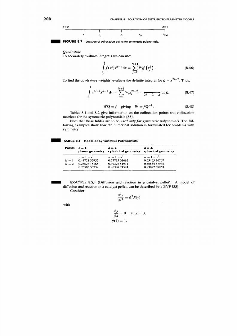
8/17/2019 Process Modelling and Model Analysis-Hangos-Cameron
http://slidepdf.com/reader/full/process-modelling-and-model-analysis-hangos-cameron 225/560
2 0 8 CHAPTER 8 SO LUT ION OF DISTRIBUTED PARAMETER MODELS
x=0 x=l
I I \ I I
Xy X2 Xj Xj^ X^^^
j i m i l F I G U R E 8.7 Location of collocation points for symmetric polynomials.
Quadrature
To accurately evaluate integrals we can use:
/
' N+l
f{x^)x''-
' (k = £ W,/
(xj) .
(8.46)
0 J='
To find the quadrature weigh ts, evaluate the definite integral for ^
= x^ ^,
Thus,
i-l
f ^+1 1
j c ^ ' -V "^ djc = V Wjxf-^
= =fi,
(8.47)
0 •^~*
WQ=f giving W=fQ-\ (8.48)
Tables 8.1 and 8.2 give information on the collocation points and collocation
matrices for the symmetric polynomials [55].
Note that these tables are to be used only for symm etric polynomials. The fol
lowing examples show how the numerical solution is formulated for problems with
symmetry.
TA BL E 8.1 Roots of Sy m m etr ic Polynomials
Points
A^= 1
N = 2
a= 1,
planar geometry
H- = 1 -
X^
0.44721 35955
0.28523 15165
0.76505 53239
a = 2,
cylindrical geometry
H- = 1 -
X^
0.57735 02692
0.39376 51911
0.80308 71524
0 = 3,
spherical geometry
w= \-x^
0.65465 36707
0.46884 87935
0.83022 38963
EXAMPLE 8.5.1 (Diffusion and reaction in a catalyst pellet). A model of
diffusion and reaction in a catalyst pellet, can be described by a BVP [55 ].
Consider
d^y 0
with
dy
- f = 0 at jc = 0,
QX
y(l) = l .
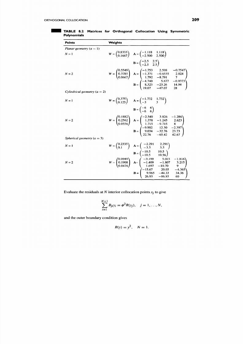
8/17/2019 Process Modelling and Model Analysis-Hangos-Cameron
http://slidepdf.com/reader/full/process-modelling-and-model-analysis-hangos-cameron 226/560
ORTHOGONAL COLLOCATION 2 0 9
• H i TABLE 8.2 Matrices for Orthogonal Collocation Using Symm etric
Polynomials
Points Weights
Planar geometry
{a = I)
/0 .8333 \ j,_(-l.nS
1.118\
1^0.1667/ ~ V-2 .500 2 .50 0/
B-(:^;?
S )
(
0.5549\ /-1.753 2.508 -0.7547^
0.3785
A =
-1.371 -0.6535 2.024
0.0667/
\ 1.79 2
-8.791
7
-4.740 5.677 -0.937 3^
8.323 -2 3. 26 14.94
^ 19.07 -4 7. 07 28
Cylindrical geometry
(a
= 2)
0.1882\ /- 2 . 54 0 3.826 -1 .28 6\
0.2562 A = 1.378 -1 .2 45 2.623
0.05 56/ \ 1.715 -9 .7 15 8
j
-9.902 12.30 -2 .39 7 >
B = I 9.034 -3 2. 76 23.73 ,
22.76 -65.42 42.67
Spherical geometry (a = 3)
L2333\
N=l W
= 2:
/0.0949
N = 2 W^= 0.1908
\ 0.0476
Evaluate the residuals at
N
interior collocation points
Xj
to give
A^+1
/=i
and the outer boundary condition gives
R(y)=y^, N = L

8/17/2019 Process Modelling and Model Analysis-Hangos-Cameron
http://slidepdf.com/reader/full/process-modelling-and-model-analysis-hangos-cameron 227/560
210
CHAPTER
8
SOLUT ION OF DISTRIBUTED PARAMETER MODELS
We have from the residual equations
Bny\-\-Bi2y2 =
(l>^R(y\)
=
(t>Vi
with
yi = 1-
For planar geometry a = 1 and for w = I
—
x ^, we have in Table 8.2
f i l l = - 2 . 5 Wi=5/6,
Bn =
2.5
W2
= 1/6.
The residual equation becomes
-2.5yx+2.5y2=(t>V^, J2 - 1.
Solve for j i = / (0^) giving
-2.5 + >/6.25 + 1002
'' =
20^ •
• • I This provides a good solution upto 0 = 2.
• • • EXAMPLE 8.5.2 (A reactor problem). Consider the following reactor problem
given by
^ ^ ( ^ - . g ) , „ ^ „ , „ . . ,
withdj/djc = 0atjc = 0; j( l)
= \,a=\.
The residuals at the collocation points are
If at jc = 1 we had — dy/dx = aj + ^ as the boundary condition, then we would
write the additional residual equation:
If we need to solve for another point (not a collocation point), then w e can use
i=\
and
d = Q - V
Note that we do not expand the Laplacian
\/^y
when using the trial functions
with symmetry built into them. Tables 8.1 and 8.2 give the matrices A and B for the
three types of geometry. When a = 1 we still use the matrices B when writing the
residuals, since the geometry information is built into the polynomials.
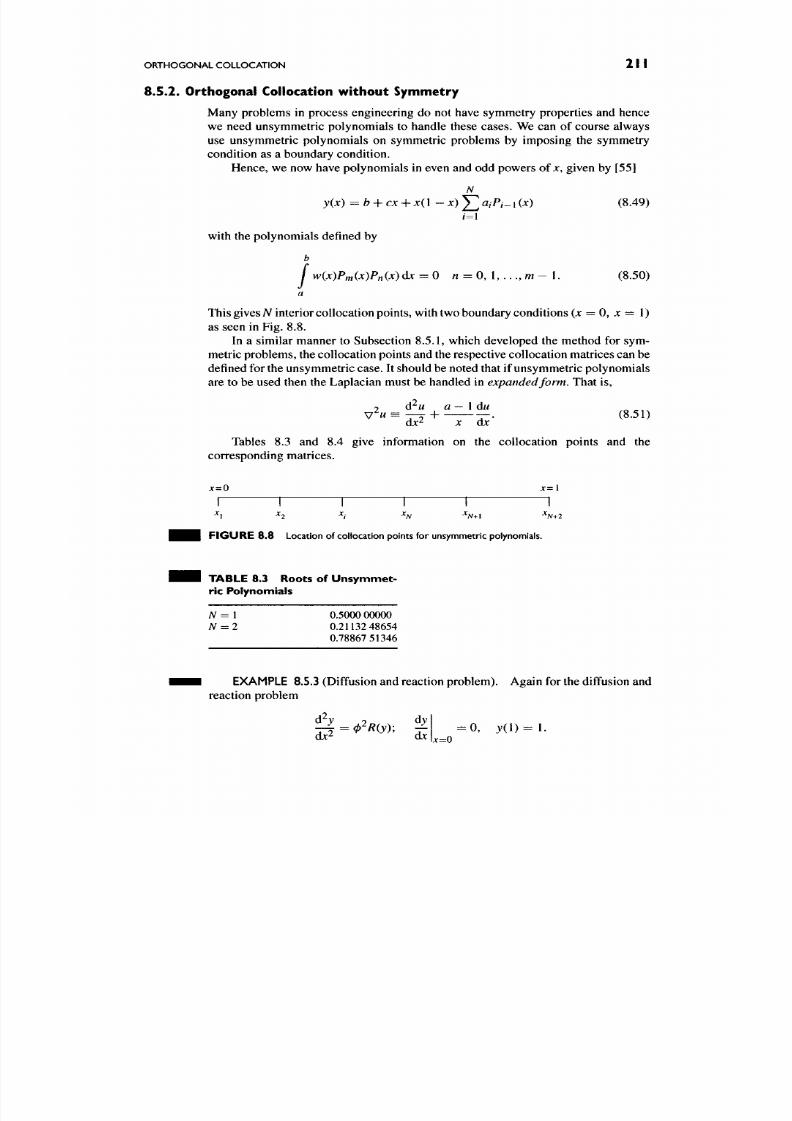
8/17/2019 Process Modelling and Model Analysis-Hangos-Cameron
http://slidepdf.com/reader/full/process-modelling-and-model-analysis-hangos-cameron 228/560
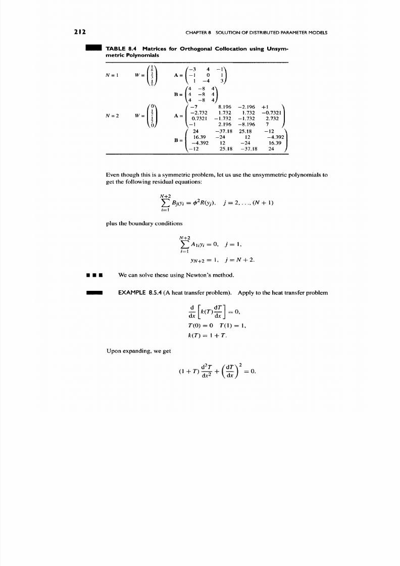
8/17/2019 Process Modelling and Model Analysis-Hangos-Cameron
http://slidepdf.com/reader/full/process-modelling-and-model-analysis-hangos-cameron 229/560
212
CHAPTER 8 SOLUTION OF DISTRIBUTED PARAMETER MODELS
TA BL E 8.4 Mat r ices for Or tho gon a l Co l loca t ion us ing Un sym -
metr ic Polynomials
A^ = l
A^ = 2
W =
W =
1
2
I
2
Vo/
/ - 3 4
-l\
A= -1 0 1
V 1 - 4
3J
/ 4 -8 4 \
B= 4 -8 4
\ 4 - 8 4 /
A =
/ - 7
-2.732
8.196
1.732
-2.196 +1
1.732 -0.7321
0.7321 -1.732
\- \ 2.196
/ 24
16.39
-4.392
V-12
1.732
8.196
-37.18 25.18
-24 12
12 -24
25.18 -37.18
2.732
7
- 1 2
-4.392
16.39
24
Even though this is a symmetric problem, let us use the unsymmetric polynomials to
get the following residual e quations:
N+2
plus the boundary conditions
J2Bjiyi =
(l>^R(yjl y = 2 , . . . , ( A ^ + l )
N-\-2
/ = l
W+ 2 = l , 7= A ^ + 2 .
We can solve these using Newton's method.
EXAMPLE 8.5.4 (A heat transfer problem) . Apply to the heat transfer problem
7'(0) = o r ( i ) = i ,
k(T) = l + T.
Upon expanding, we get
m'-o-

8/17/2019 Process Modelling and Model Analysis-Hangos-Cameron
http://slidepdf.com/reader/full/process-modelling-and-model-analysis-hangos-cameron 230/560
ORTHOGONAL COLLOCATION 2 I 3
This is an unsymmetric problem and we have to use unsymmetric polynomials to get
the residual equations
N-\-2
W4-2
E'^i'^'
2
0 , 7 = 2 , . . . , ( A ^ + 1 )
/ • = l
together with the boundary conditions
7 1 = 0 ,
rA^+2 = l .
Onc e we specify the number of internal collocation points, w e can set up the equations
and solve for the unknowns.
For
A^
= 1, we have
7 = 2
/= l \ / = i /
(1 +
T2)
(471 - 872 + 473) + ( - 7 i +
T^f =
0
with
^ 1 = 0 73 = 1,
giving
72 = 0.579.
8.5.3. Orthogonal Collocation on Elements
In cases like the diffusion-reaction problem where the profiles can be very steep , it
can be of advantage to divide the region into elements and use orthogonal colloca
tion on separate elements rather than one polynomial over the whole region (global
collocation).
It is then possible to reduce the number of total collocation points. This can
significantly reduce computation time.
To do this, we use trial functions plus continuity conditions across the element
boundaries. We use
unsymmetric
polynomials since we do not want to impose the
symmetry condition on each element.
Setting up the problem
We divide the global
x
domain into a number of elements. A typical element exists
between Xk and
X]^j^\.
This situation is shown in the Fig. 8.9.
Hence,
^Xk=XkJ^x-Xk (8.52)
and NE = total number of elements.
At the end points of each element, we want the function and the first derivative
to be equal to the adjacent element and continuous across the element boundary.
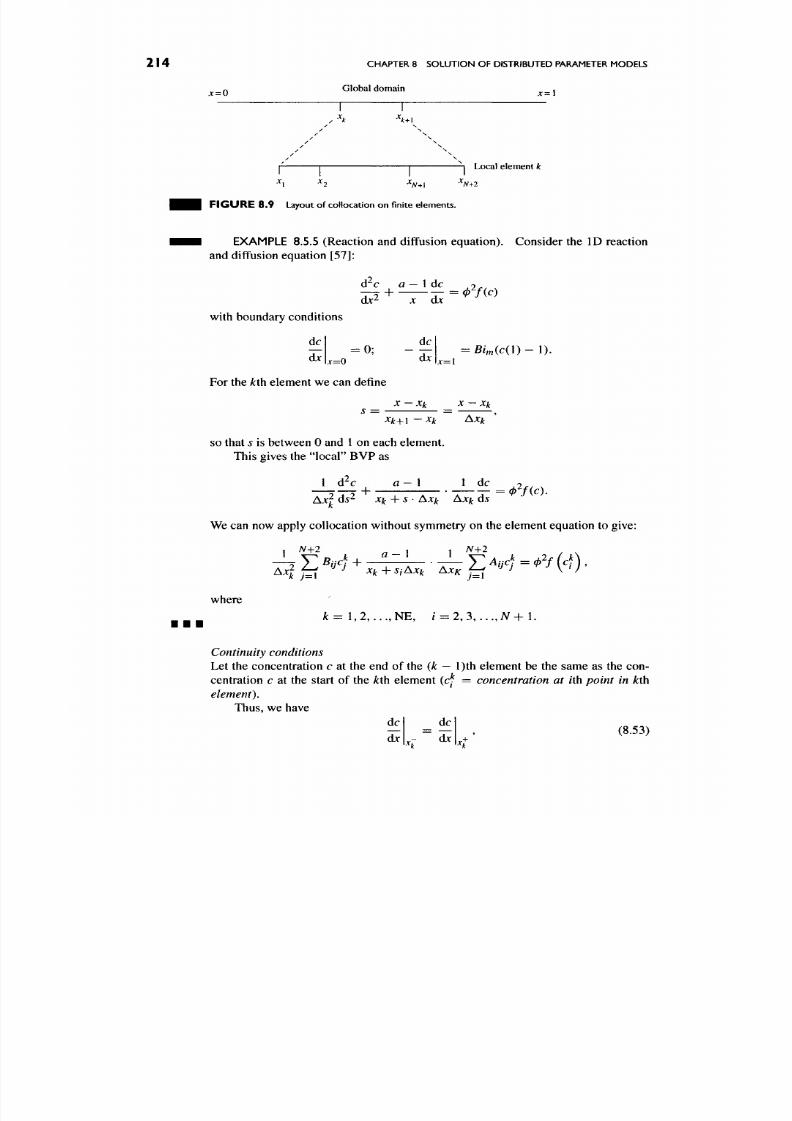
8/17/2019 Process Modelling and Model Analysis-Hangos-Cameron
http://slidepdf.com/reader/full/process-modelling-and-model-analysis-hangos-cameron 231/560
214
j c=0
CHAPTER 8 SO LUT ION OF DISTRIBUTED PARAMETER MODELS
Globa l domain _ .
-"jt+i
Local e lement
k
F I G U R E 8 .9 Layout of col location on f ini te elements.
EXAMPLE 8.5.5 (Reac tion and diffusion equation). Consider the ID reaction
and diffusion equation [57]:
d^c
a
—
\ dc 2
djc2
+
X djc
=
rfic)
with boundary conditions
d c
due
= 0 ;
;c=0
d£
dbc
Birn(ci\)-\).
x=\
For the
A;th
element we can define
s =
X
— Xk X-Xk
Xk+{ -Xk Axk
so that
s
is between 0 and I on each element.
This gives the "local" BVP as
1 d^c
+
a - \
1 dc
Axj ds^ Xk-\-s- Axk Axk ds
= rfic).
We can now apply collocation without symmetry on the element equation to give:
N+l
Ax]
E M
+
a-l
N+2
X:A,c;^^V(cf),
where
ij^\
-^^+
^^^^ ^^ ^ j^i
k=:
1,2,...,NE, / = 2 , 3 , . . . , A ^ + 1 .
Continuity
conditions
Let the concentration c at the end of the (k — l)th element be the same as the con
centration c at the start of the
kih
element
(c^ = concentration at iih point in kih
element).
Thus, we have
del
d b c l
del
dx\
(8.53)
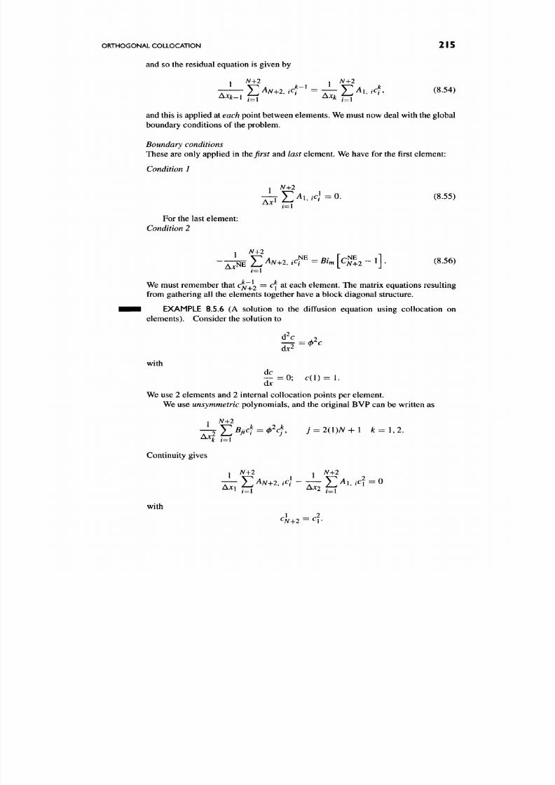
8/17/2019 Process Modelling and Model Analysis-Hangos-Cameron
http://slidepdf.com/reader/full/process-modelling-and-model-analysis-hangos-cameron 232/560
ORTHOGONAL COLLOCATION
2 I 5
and so the residual equation is given by
1
A^+2 . A^+2
S5:;E' .«.4-'=^g^..-c?.
8 . 5 4 )
and this is applied at each point between elem ents. We must now deal w ith the global
boundary conditions of the problem.
Boundary conditions
These are only applied in
iht first
and
last
elemen t. We have for the first element:
Condition 1
1 N-\-2
— ^ ^ A i , , c / = 0 . (8.55)
For the last element:
Condition 2
-^ J2 ^N-,2, icf^ = Bim kN^2
-
1
•
^^'^^^
We must remember that Cj^^2 ~ ^\ ^ ^^^^ element. The matrix equations resulting
from gathering all the elements together have a block diagonal structure.
EXAMPLE 8.5.6 (A solution to the diffusion equation using collocation on
eleme nts). Con sider the solution to
with
dc
_ = 0 ; c ( l ) = l.
QX
We use 2 elements and 2 internal collocation points per element.
We use
unsymmetric
polynomials, and the original BVP can be written as
— 2 ^ 5 y 4 = 02^j^, y = 2 ( l) A ^ + l ^ = 1 , 2 .
Continuity gives
with
I iV+2
J A^+2
^1
_^ 2
%+2 - ^\'

8/17/2019 Process Modelling and Model Analysis-Hangos-Cameron
http://slidepdf.com/reader/full/process-modelling-and-model-analysis-hangos-cameron 233/560
2 I 6
CHAPTER
8
SOLUTIO N OF DISTRIBUTED PARAMETER MODELS
The boundary conditions are as follows:
1 N+2
Hence, the matrix equations are
/A n Ai2 Ai3 Au
Bix B22 B23 B24
^ 3 1
^ 3 2 ^ 3 3 ^ 3 4
A41
A42 A43
(A44_Aii)
^31
V
/ 0 \
0
2^2^2
1
Ax^^^c^
where
-All
B22
Bii
- A i 3
B23
B33
\
--414
^24
B34
1 /
Ah
1 c'
^ 3
1 ^
1 '^2
c2
1
^
1^2
^ 1
_ ^2
The matrix equation can then be solved using a Newton-like iteration to solve
for the unknown concentrations Cj to c^ .
8.6. ORTHOGONAL COLLOCATION FOR PARTIAL DIFFERENTIAL EQUATIONS
Orthogonal collocation can be easily applied to transient problems to produce a set
of ODE initial value problems. This follows the development by Finlayson [57].
For the general PPDE , we can use a similar development of the non-symmetrical
trial function but now the coefficients are functions of t. That is,
y{x,t) = b(t) -\- c (t)x -]- xi\ - x )Y]ai (t) Pi-.\ (x) ,
which can be written as
A^+2
y{xj)= J2diit)x'
- 1
(8.57)
(8.58)

8/17/2019 Process Modelling and Model Analysis-Hangos-Cameron
http://slidepdf.com/reader/full/process-modelling-and-model-analysis-hangos-cameron 234/560
ORT HOG ONA L COL LOC ATIO N FOR PARTIAL DIFFERENTIAL EQUATIONS 2 17
At the collocation points jcy, w e would have
y(xj, t)=J2
^/(O^j"^
=>
y(t)
=
Qd(t),
(8.59)
with
dy(xj,t) %±^ i . dy
- ^ ^
= J2diit){i-l)xp^=^^ = Cd{t),
(8.60)
\7^y = Dd(t).
(8.61)
Hence, for the transient problem in one dimension, the formulation is identical
to the boundary value problem except that the coefficients are changing with time.
This means we will have sets of ODEs to solve.
^ • H EXAMPLE 8.6.1 (No nlinear diffusion and reaction problem ). Cons ider the
following one dimensional problem given by:
du
Jt
with boundary cond itions:
M(0,
0 = 1
M ( 1 , 0 = 0
and initial conditions:
M(JC, 0) = 0
For this problem, we can write the collocation equations as
^^. A^+2 Ar+2
- ^ = ^ A ^ 7 / ) ( w / ) J ] ^ ' - ^ " ^ + ^ ( " y ) ' 7 = 1 , . . . , A ^ (8.62)
or
^=D {uj)'^^BjiUi + ^f-\T^Ajiuj +R{uj), j^h...,N
(8.63)
8/17/2019 Process Modelling and Model Analysis-Hangos-Cameron
http://slidepdf.com/reader/full/process-modelling-and-model-analysis-hangos-cameron 235/560
2 18
CHAPTER
8
SOLUTIO N OF DISTRIBUTED PARAMETER MODELS
with the usual boundary conditions:
w, (0 = 1,
UN^2{t)=0.
(8.64)
• • • We can solve these OD Es using standard packages.
8 7 .
SUMMARY
This chapter has considered a wide range of nunierical methods for the solution
of various types of PDEs. The most well known of the methods are those based
on PDAs for the terms in the PDEs. These are conceptually simple and relatively
easy to implement. A range of classes were discussed which covered both explicit
and implicit methods. The implicit methods allow larger discretizations to be made
without breaching stability bounds.
The method of lines is a useful technique which converts PPDEs into sets of
ODEs. The problem can then be easily solved using standard integrators.
Finally,
we
considered
a
polynomial approximation method based
on
collocation.
This is a powerful techn ique and easily applied to all classes of PDEs. It is conceptually
more difficult but implementation is straightforward. It is widely used in the process
industries for the solution of these types of problems.
8.8. REVIEW QUESTIONS
Q8.1. What are the three classes of PDE s encountered in process engineering appli
cations? Give some examples of when and where these equation classes arise.
(Section 8.1)
Q8.2. Describe the principal categories of numerical methods for the solution of
PDE systems. (Section 8.1)
Q8.3.
Wh at are the steps needed in applying the finite difference method to the
solution of PDE models? What key forms of finite difference methods exist and
what are the characteristics of each in terms of stability and complexity of solution?
(Section 8.2)
Q8.4.
Wh at is the advantage of using some form of implicit method in the solution
of PDEs using finite difference metho ds? Wh en is it necessary? (Section 8.2.2)
Q8.5. What is the method of lines and what properties of the method does one need
to consider in using it? (Section 8.3)
Q8.6.
Wh at are the key conce pts behind the method of weighted residuals? Describe
the steps in applying the technique to a problem. (Section 8.4)
Q8.7. Wh at is special about orthogonal polynom ials that make them useful for
applying the method of weighted residuals to a problem? (Section 8.5)
Q8.8.
Describe the approach needed in applying the orthogonal collocation tech
nique to the general solution of PDEs? (Section 8.6)
Q8.9. Describe some techniques for handling the solution of 2D and 3D PDE
models.
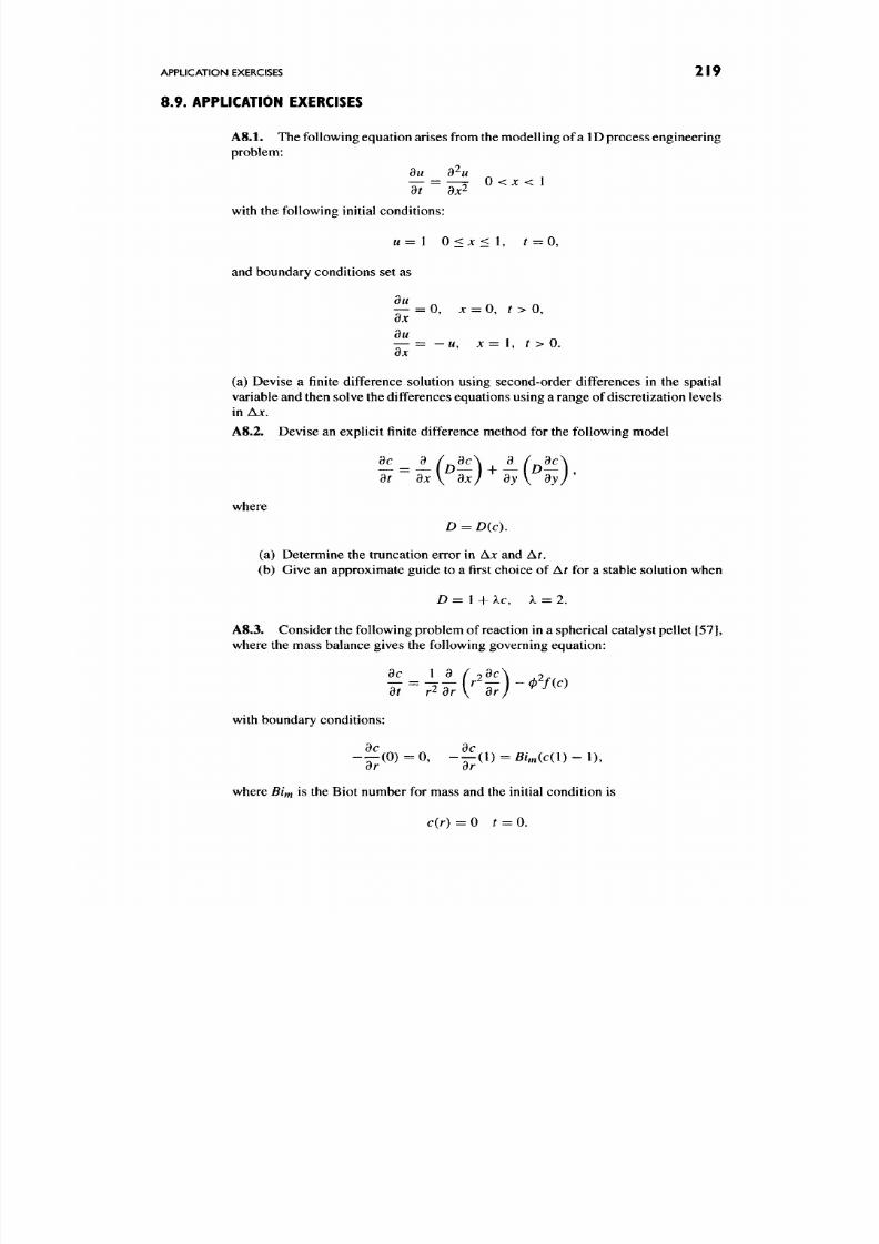
8/17/2019 Process Modelling and Model Analysis-Hangos-Cameron
http://slidepdf.com/reader/full/process-modelling-and-model-analysis-hangos-cameron 236/560
APPLICATION EXERCISES
2 19
8.9. APPLICATION EXERCISES
A8.1.
The following equation arises from the mod elling of a
1D
process engineering
problem:
du d^u
— = — ^ 0 < j c < 1
with the following initial conditions:
u= I 0 < j c < l , r = 0,
and boundary conditions set as
9w ^ ^ ^
— = 0, jc = 0, r > 0,
dx
^ "
—
—
—
u, X = I, t > 0.
dx
(a) Devise a finite difference solution using second-order differences in the spatial
variable and then solve the differences equations using a range of discretization levels
in Ax,
A8.2.
Devise an explicit finite difference method for the following model
— - —
(D—\
—
(D—\
where
D = D{c).
(a) Determ ine the truncation error in
Ax
and
At.
(b) Give an approximate guide to a first choice of Af for a stable solution w hen
D =
1
-h Xc,
A
= 2.
A8.3. Con sider the following problem of reaction in a spherical catalyst pellet [57],
where the mass balance gives the following governing equation:
dc \ d / ^dc\ 9
with boundary conditions:
dc dc
- - ( 0 ) = 0, - - ( 1 ) = BiUcH) - 1),
dr dr
where
Bim
is the Biot number for mass and the initial condition is
c{r)
= 0 r = 0 .
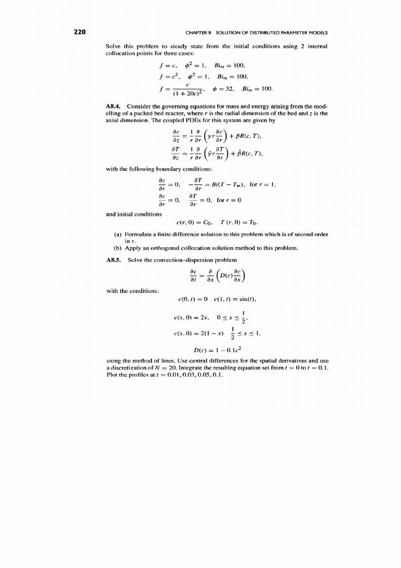
8/17/2019 Process Modelling and Model Analysis-Hangos-Cameron
http://slidepdf.com/reader/full/process-modelling-and-model-analysis-hangos-cameron 237/560
220
CHAPTER
8
SOLUT ION OF DISTRIBUTED PARAMETER MODELS
Solve this problem to steady state from the initial conditions using 2 internal
collocation points for three cases:
/ = c, 0^ = 1,
Bim = 100,
f = c^,
0^ = 1, Bhn
= 100,
A8.4. Consider the governing equations for mass and energy arising from the mod
elling of a packed bed reactor, where r is the radial dimension of the bed and
z
is the
axial dimension. The coupled PDEs for this system are given by
dz rdry drj
^ ^ ' ^'
with the following boundary conditions:
^ = 0 , -—=Bi{T-T^), f o r r = l ,
dr or
dc dT
— = 0, — = 0, for r = 0
dr dr
and initial conditions
c( r ,0 ) = Co, r ( r , 0 ) = 7b.
(a) Formu late a finite difference solution to this problem which is of second order
in r.
(b) Apply an orthogonal collocation solution method to this problem.
A8.5.
Solve the conv ection-disp ersion problem
with the conditions:
dc
Jt
c(0, t)
-.
c{x,
0) =
c{x,
0) =
d
= 0
2x,
2 ( 1 -
D{c) =
HS)
c ( l , 0 = s i n ( 0 ,
0<x<\,
-x )
~ <j c < 1,
2 ~ ~
1-O.lc^
using the method of lines. Use central differences for the spatial derivatives and use
a discretization ofN = 20. Integrate the resulting equation set from r = 0 to f = 0. 1 .
Plot the profiles at
t ==
0 .01 ,0 .03 ,0 .05 ,0 .1 .
8/17/2019 Process Modelling and Model Analysis-Hangos-Cameron
http://slidepdf.com/reader/full/process-modelling-and-model-analysis-hangos-cameron 238/560
APPLICATION EXERCISES
22 I
A8.6. Cons ider the following problem which arises from the mo delling of axial and
radial diffusion in a tubular reactor. The energy balance gives
\ 1 d^T
T a d / dT\ 1 d^T
dz r dr \ dr J Pe dz^
The radial dimension boundary conditions are given by
dT dT
—-=0
atr = 0,
—T-=Biy,^ii(T(\,z)-Ty,^n)
at r = 1
dr dr
and the axial dimension conditions could be
dT dT
— =Pe(T- 1) a t z = : 0 , — = 0 a t z = 1.
dz dz
(a) Devise an orthogon al collocation solution to this problem .
(b) Apply a finite difference solution to this problem.
A8.7.
For the general nonlinear parabolic diffusion equation in one dimension is
given by
dc _ d / dc\
dt dx\ dxj
with initial condition
and boundary co nditions
c(jc, 0 ) = 0
c(0,t) = 1, c ( l , 0 = 0 .
(a) Devise a finite difference schem e of second order in the spatial variable for
the solution. Solve it for a range of spatial discretization levels.
(b) Develop a global orthogonal collocation solution to this problem and solve
it for two different num bers of internal points.
(c) Consider the formulation of the orthogonal collocation solution on several
elements.
A8.8 For the model of the double pipe heat exchanger given in Example 7.2.1.
(a) Develop a numerical solution based on a finite difference approac h. Test the
method by solving the problem over the exchanger length of 10 m for a series
of discretizations in Az ranging from 0.1 to 1.0. Comment on the solution
accuracy.
(b) Try solving the problem using orthogonal collocation and compare the results
to those of the
finite
difference m ethods . Can a few collocation points produc e
an acceptable solution?
Assume reasonable values for all unspecified parameters. Use physical
properties relevant to water for the fluids.
A8.9.
For the mod el of the pollutant dispersion in a river given in Exam ple 7.2.3.

8/17/2019 Process Modelling and Model Analysis-Hangos-Cameron
http://slidepdf.com/reader/full/process-modelling-and-model-analysis-hangos-cameron 239/560
222 CHAPTER 8 SOLUTIO N OF DISTRIBUTED PARAMETER MODELS
(a) Set up a numerical solution of the problem using a finite difference approach
and solve it for a range of spatial discretizations. Comment on the behaviour of the
solution as a function of discretization and timestep.
(b) Use the method of lines to set up the OD Es to simulate the behaviour of the model.
Investiga te the effect of spatial discre tization on the solution as well as the integration
accuracy. Use MATLAB to carry out the solution.
Assume reasonable values for all unspecified parameters.

8/17/2019 Process Modelling and Model Analysis-Hangos-Cameron
http://slidepdf.com/reader/full/process-modelling-and-model-analysis-hangos-cameron 240/560
PROCESS MODEL HIERARCHIES
For even a mod erately com plicated proc ess system , there is usually a set of different
models for the same purpose that describe the system in different detail and/or at
different
levels.
These m odels are not independ ent of each other but are related through
the process system they describe and through their related modelling goals. One may
arrange these models in a hierarchy:
• Starting from a static model with only the input and output variables of the
process system through to the most detailed dynamic distributed parameter
model which includes all the controlling mechanisms. This is a hierarchy
driven by the level of detail.
• Starting from the molecular level, describing elementary molecu lar kinetics to
the most detailed dynam ic distributed param eter model w ith all the controlling
mechanisms d escribed. This is
a
hierarchy
driven by c haracteristic sizes
which
is used in multi-scale modelling. It spans the nano to the macro scale.
• Starting from the mod els describing the slowest mo de of the process system
to the models incorporating the fastest modes. This is a
hierarchy driven by
characteristic times.
Hierarchies are driven by basic or fundamental modelling assumptions affecting
• the balance volum es, their numb er and type (lumped or distributed),
• the system boundaries or the focus of mod elling,
• one or more basic controlling mec hanism s, such as diffusion, presen t in most
of the balance volumes in the process system.
223

8/17/2019 Process Modelling and Model Analysis-Hangos-Cameron
http://slidepdf.com/reader/full/process-modelling-and-model-analysis-hangos-cameron 241/560
224
CHAPTER 9 PROCESS MO DEL HIERARCHIES
These are all general composite assump tions specified for the overall system .
Figure 9.1 shows schematically the model space defined by such mu lti-scale mod
elling concepts. Any model M(J,
s, t)
can be located within the multi-scale domain
and families of models can then be developed by moving along one of the characteristic
co-ordinate axes.
Together with the hierarchies various ways of obtaining one model in the hier
archy from another one are also described. These methods can also be seen as
model simplification or model enrichment techniques.
Characteristic times (/)
Characteristic sizes
{s)
Characteristic details {d)
F I G U R E 9 .1 Mult i-scale mode ll ing domain.
These hierarchies and the transfer of information between levels is described in
this chapter and illustrated on the example of a packed bed catalytic reactor. The
problem statement of the modelling task of the packed bed tubular catalytic reactor
is given in Exam ple
9.0.1.
Note that the same process system was used in Chapter 7 in Example 7.1.1 to
illustrate the development of distributed parameter models.
EXAMPLE 9.0.1 (M odelling of a simple packed bed tubular catalytic reac tor).
Process system
Consider a tubular reactor completely filled with catalyst and with ideal plug flow.
A pseudo-first-order catalytic reaction A ->• P takes place in an incom pressible fluid
phase.
The process is shown in Fig. 9.2.
Modelling goal
Describe the behaviour of the reactor for design purposes.
From the problem description above, we may extract the following modelling
assumptions which will be generally valid for any further model we derive in this
chapter.

8/17/2019 Process Modelling and Model Analysis-Hangos-Cameron
http://slidepdf.com/reader/full/process-modelling-and-model-analysis-hangos-cameron 242/560
HIERARCHY DRIVEN BY THE LEVEL OF DETAIL
225
F I G U R E 9 . 2 Simple tubular catalytic plug flow reactor.
Assumptions
^ 1 . Plug flow is assumed in the reactor, which has constant volume.
Al. A pseudo-first-order reaction A-^ P takes place.
^ 3 .
An incom pressible (liquid) phase is present as a bulk phase .
^ 4 . A solid phase catalyst is present which is uniformly distributed.
9 .1 . HIERARCHY DRIVEN BY THE LEVEL OF DETAIL
In order to capture the idea of how different models describing the same process
system with different level of detail relate to each other, let us imagine a process system
which w e view from different (spatial) distances. In principle, we are able to see finer
detail as we get closer to the system. We shall arrange the models corresponding to
different levels of magnification, so that the different granularity reflects
hierarchy
levels driven by detail. The more detail we take into account, the lower the level of
model we consider. The number of levels varies according to the complexity of the
process system and according to the modelling goal.
The sequence of models in this hierarchy is naturally developed if one performs
a process engineering design of a system in a top-do wn approach. First, the process
functionality and its connection to the environment is defined as a top level model.
Therefore, the flowsheet is developed with the necessary operating units and their
connection forming a middle level model. Finally, the detailed design is performed
with a bottom level model with all the necessary details.
9 . 1 . 1 . Hierarchy levels driven by detail
In the following, we shall illustrate the characteristics and relationship of models at
different hierarchy levels which are driven by detail. Th is will be illustrated on a simple
case with only three levels. Here, we have a
top, middle
and
bottom level.
Figure 9.3
shows schematically the model hierarchy in relation to one of the characteristic co
ordinates.

8/17/2019 Process Modelling and Model Analysis-Hangos-Cameron
http://slidepdf.com/reader/full/process-modelling-and-model-analysis-hangos-cameron 243/560
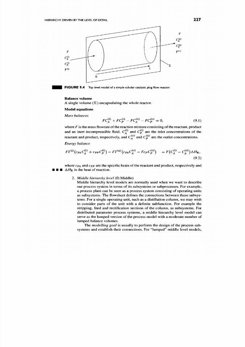
8/17/2019 Process Modelling and Model Analysis-Hangos-Cameron
http://slidepdf.com/reader/full/process-modelling-and-model-analysis-hangos-cameron 244/560
HIERARCHY DRIVEN BY THE LEVEL OF DETAIL
227
FI G U R E 9.4 Top level model of
a
simple tubular catalytic plug flow reactor.
Balance volume
A single volume ( E ) encapsulating the whole reactor.
Model equations
Mass balances
FCf^FCf-FCf
FCf = 0,
(9.1)
where F is the mass flowrate of the reaction mixture con sisting of the reactant, produ ct
and an inert incom pressible fluid. Q and
Cp
are the inlet conce ntrations of the
reactant and produc t, respectively, and Q ^ and Cp are the outlet conc entrations.
Energy balance
FT^'^icpACf + cppCf) - FT<-\cpACf - FcpCf) = F{C^^ - c f ) A / / R ,
(9.2)
where cpA and
c pp
are the specific heats of the reactant and product, respectively and
A / / R
is the heat of reaction.
2.
Middle hierarchy level
(D.Middle)
Middle hierarchy level models are normally used when we want to describe
our process system in terms of its subsystems or subprocesses. For example,
a process plant can be seen as a process system consisting of operating units
as subsystems. T he flowsheet defines the connections between these subsys
tems. For a single operating unit, such as a distillation column, we may wish
to consider parts of the unit with a definite subfunction. For example the
stripping, feed and rectification sections of the column, as subsystems. For
distributed parameter process systems, a middle hierarchy level model can
serve as the lumped version of the process model with a moderate number of
lumped balance volumes.
The
modelling goal
is usually to perform the design of the process sub
systems and establish their connections. For "lum ped" middle level mo dels.

8/17/2019 Process Modelling and Model Analysis-Hangos-Cameron
http://slidepdf.com/reader/full/process-modelling-and-model-analysis-hangos-cameron 245/560
228
CHAPTER 9 PROCESS MO DEL HIERARCHIES
the goal is often to describe the dynamic in put-o utput behaviour of the process
system.
The
balance volume
set is usu ally driven by the subsystem decom position.
Here, we allocate at least one balance volume for each of the subsystems.
For distributed param eter models we define perfectly mixed balance vo lumes
for each lumped subsystem. It is
important to note that the union
of all
the
balance volumes
in
the middle level model
is
the balance volum e
of the
top
level model.
We only consider convection and transfer without time delay
between the balance volumes.
As an example of a middle hierarchy level model driven by detail, we
describe a lumped version of the distributed bottom level model of the simple
packed bed tubular catalytic reactor introduced in Example
9.0.1.
EXAMPLE 9.1.2 (Lumped middle level model
of a
simple packed
bed
tubular
catalytic reactor).
Process system
Consider a plug flow tubular reactor completely filled with catalyst and with a pseudo
first-order A
-^ P
catalytic reaction.
The
flowsheet with
the
balance volumes
and
process variables is shown in Fig. 9.5.
Modelling goal
To describe the approximate dynamic input-output behaviour of the reactor for
design purposes.
Assumptions
a dditional to the ones listed as
1-4
are the following:
A5. The reactor is described as
a
sequence of three CST Rs.
A6,
Adiabatic conditions apply.
Al.
Constant physico-chem ical properties.
^ 8 . Uniform initial conditions in the reactor.
Balance volumes
We consider three balance volumes
(Ej
equal holdups and
(D.Middle) ^(D.Middle)
and
E
(D.Middle)
) with
F I G U R E 9. 5 Lumped model of the catalytic plug f low reactor.
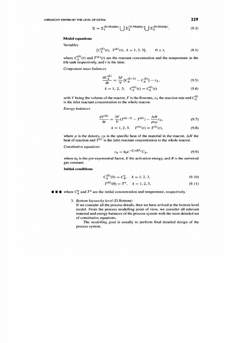
8/17/2019 Process Modelling and Model Analysis-Hangos-Cameron
http://slidepdf.com/reader/full/process-modelling-and-model-analysis-hangos-cameron 246/560
HIERARCHY DRIVEN BY THE LEVEL OF DETAIL
229
v _ v(D.M iddle) I I y,(D.Middle) I I y,(D.Middle) .g ^.
Model equations
Variables
{Cf(t),
T^'^Ht), k=h2,3), 0 < r, (9.4)
where Q \t ) and
T^^\t)
are the reactant concentration an d the temperature in the
/:th tank respectively, and
t
is the time.
Component mass balances
f - = Y{Cr '-Cr) -rA, (9.5)
k = l,2,
3 ,
Cfit)
= C j ' (0 (9.6)
with V being the volume of the reactor,
F
is the flowrate, r^ the reaction rate and Q
is the inlet reactant concentration to the whole reactor.
Energy balances
dr
V pep
A: = 1 , 2 , 3 ,
T^''Ht)
= T^^(t), (9.8)
where
p
is the density,
cp
is the specific heat of the material in the reactor,
AH
the
heat of reaction and T^^ is the inlet reactant concentration to the whole reactor.
Constitutive equations
rA=koc-^^^'^^^CA,
(9.9)
where k o is the pre-exp onential factor, E the activation energy, and R is the universal
gas constant.
Initial conditions
Cf(0) = cl, k = 1,2,3,
(9.10)
r^^)(0) = r*,
k=
1,2,3, (9.11)
• • • where C^ and T* are the initial concentration and temperature, respectively.
3.
Bottom hierarchy level
(D.Bottom)
If we consider all the process d etails, then we have arrived at the bottom level
model. From the process modelling point of view, we consider all relevant
material and energy balances of the process system with the most detailed set
of constitutive equations.
The modelling goal is usually to perform final detailed design of the
process system.

8/17/2019 Process Modelling and Model Analysis-Hangos-Cameron
http://slidepdf.com/reader/full/process-modelling-and-model-analysis-hangos-cameron 247/560
230 CHAPTER 9 PROCESS MODEL HIERARCHIES
Here, we have the finest balance volume set. For process systems with
only lumped (perfectly m ixed) subsystems, we have balance volumes for every
perfectly mixed holdup and for every phase in the system. For distributed
parameter process systems, we set up balance volumes for every holdup of
the same type of spatial distribution and for every phase or we lump the system
into a high number of perfectly mixed balance volum es.
Here again the union
of all the balance volumes in the bottom level model is the balance volume
of
the
top level model as driven by detail
We consider only convection and
transfer without time delay between the balance volumes.
An exam ple of a distributed, bottom hierarchy level model of the simple
packed bed tubular catalytic reactor introduced in Example 9.0.1 is as follows.
• • • EXAMPLE 9.1.3 (Distributed bottom level model of a simp le packed bed tubular
catalytic reactor).
Process system
Consider a plug flow tubular reactor completely filled with catalyst and a pseudo
first-order catalytic reaction A -> P. The flowsheet is the same as shown in Fig. 9.2.
Modelling goal
To describe the overall behaviour of the reactor for final design purp oses.
Assumptions Additional to the ones listed as 1 -4 are the following:
A5. The reactor is uniformly d istributed in its cross section, and no radial
diffusion or convection takes place.
A6.
Adiabatic conditions apply.
Al. Constant physico-ch emical properties.
^ 8 .
No diffusion in the axial direc tion.
A9.
The initial distribution of com ponent
A
and the temperature in the reactor
is uniformly constant.
Balance volumes
A single volume (j]^'^-^^^^^"^)) encapsulating the whole reactor but this time this
balancing volume is a d istributed one.
Model equations
Variables
0 < J C < L , f > 0 , Q (j c ,0 ,
T{xJ),
(9.12)
where
x
is the spatial coordinate in axial direction,
L
the length of the reactor,
t
the
time, CA the reactant concentration and T is the temperature.
Component mass balances
^ = - F ^ - . , (9.13)
dt dx
where
F
is the mass flowrate of the inert incompressible fluid and
rA
is the
reaction rate.

8/17/2019 Process Modelling and Model Analysis-Hangos-Cameron
http://slidepdf.com/reader/full/process-modelling-and-model-analysis-hangos-cameron 248/560
HIERARCHY DRIVEN BY THE LEVEL OF DETAIL
23 I
Energy balance
dT dT AH
_ ^ , ^
— =
-F- rA
(9.14)
at ax cp
where
cp
is the specific heat of the material in the reactor and
AH
is the heat of
reaction.
Constitutive equations
rA=h^-^'^^CA, (9.15)
where A:o is the pre-exponen tial factor,
E
the activation energy, and
R
is the universal
gas constant.
Initial and boundary conditions
Q(jc, 0) = C^, CA(0 , 0 = C f , (9.16)
r(jc, 0) = r* , 7(0 , 0 =
T^'\
(9.17)
where Q and T * are the inlet concentration and the inlet tempe rature, while C |
• I • and r * are the initial concen tration and temperature, respectively.
9.1.2. The relation between models of different levels driven by detail
Modelling goal and modelling assumptions
As only the level of detail varies with changing the level in this hierarchy, the mod
elling assumptions on the system boundaries and input and output relations with its
environment are the same for the models in all levels. The basic assumptions on the
presence or absence of controlling m echanism s are also the same, such as the absence
of diffusion in the system.
The assumptions on the balance volumes are the ones characterizing a particular
level in the hierarchy driven by detail. The set of modelling assumptions on a lower
level is larger than that on a higher level. That is because additional modelling
assumptions are needed to incorporate more detail into a lower level model.
The "p recision " of the mod els on various levels can be considerably different
and the modelling goal is the one which dictates which level to choose for the given
purpose.
Balance volumes
From the above examples, we can conclude that
a balance volume of a higher hier
archy level driven by detail is obtained as a union of some balance volumes in the
lower level.
M oreover,
w(D.Middle) »r(D.Bottom)
^=^\j SJDMiddle) ^ ^ y j,(D.Bottom) ^^^^^
should also hold. That is, the union of all balance volumes in any of the hierarchy
levels (Ej'^MWdle) ^^ j,(D.Bottom)^ ^j^^^^j^ encapsulate the whole process system.
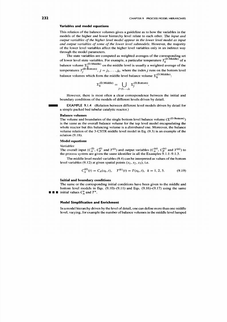
8/17/2019 Process Modelling and Model Analysis-Hangos-Cameron
http://slidepdf.com/reader/full/process-modelling-and-model-analysis-hangos-cameron 249/560
232 CHAPTER 9 PROCESS MODEL HIERARCHIES
Variables and model equations
This relation of the balance volumes gives a guideline as to how the variables in the
models of the higher and lower hierarchy level relate to each other. The input and
output variables of
the
higher level model appear in the lower level model as input
and output variables of some of
the
lower level submodels.
However, the majority
of the lower level variables affect the higher level variables only in an indirect way
through the model parameters.
The state variables are computed as weighted averages of the corresponding set
of lower level state variables. For example, a particular temperature Tj^ ' ^ ^ of a
balance volume ^l ' ^ on the middle level is usually a weighted average of the
tem peratu res 7- ^"^"^^^
j =j\,
-^
-Jk^
where the index y runs on the bottom level
balance volumes which form the middle level balance volume ^l ' ^ -
^(D.Middle ) ^ 1 1 ^ . (1(D.Middle) _ I I ^ (D.Bottom)
However, there is most often a clear correspondence between the initial and
boundary conditions of the m odels of different levels driven by detail.
EXAMPLE 9.1.4 (Relation between different level mo dels driven by detail for
a simple packed bed tubular catalytic reactor.)
Balance volumes
The volume and boundaries of the single bottom level balance volume (^(D.Bottom)^
is the same as the overall balance volume for the top level model encapsulating the
whole reactor but this balancing volume is a distributed one. Moreover, the balance
volume relation of the 3-CSTR middle level model in Eq. (9.3) is an example of the
relation (9.18).
Model equations
Variables
The overall input
(cf,
C^p^ and
T^'^)
and output variables
(C^^\
C^p^ and r^«>) to
the process system are given the same identifier in all the Examples 9.1.1-9.1.3.
The m iddle level model variables (9.4) can be interpreted as values of the bottom
level variables (9.12 ) at given spatial points (x\, JC2, JC3), i.e.
C^A^it)
= CA(xk, t),
r^^>(0 =
T{xk. t),
A = 1,2, 3. (9.19)
Initial and boundary conditions
The same or the corresponding initial conditions have been given to the middle and
bottom level models in Eqs. (9.10)-(9.11) and Eqs. (9.16)-(9.17) using the same
initial values C^ and T*.
Model Simplification and Enrichment
In a model hierarchy driven by the level of detail, one can define more than o ne middle
level, varying, for example the num ber of balance volumes in the middle level lumped
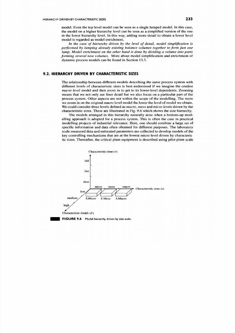
8/17/2019 Process Modelling and Model Analysis-Hangos-Cameron
http://slidepdf.com/reader/full/process-modelling-and-model-analysis-hangos-cameron 250/560
HIERARCHY DRIVEN BY CHARACTERISTIC SIZES 233
model. Even the top level model can be seen as a single lumped model. In this case,
the model on a higher hierarchy level can be seen as a simplified version of the one
in the lower hierarchy level. In this way, adding more detail to obtain a lower level
model is regarded as model enrichment.
In the case of hierarchy driven by the level of detail model simplification is
performed by lumping already existing balance volumes together to form just one
lump. Model enrichment on the other hand is done by dividing a volume into parts
forming several new volumes. M ore about model simplification and enrichm ent of
dynamic process m odels can be found in Section 13.3.
9.2 .
HIERARCHY DRIVEN BY CHARACTERISTIC SIZES
The relationship between different models describing the same process system with
different levels of characteristic sizes is best understood if we imagine the crudest
macro level
model and then zoom in to get to its lower-level dependents. Zooming
means that we not only see finer detail but we also focus on a particular part of the
process system. Other aspects are not within the scope of the modelling. The more
we zoom in on the original macro level model the lower the level of mod el we ob tain.
We could cons ider three levels defined as macro, meso and micro levels driven by the
characteristic sizes. These are illustrated in Fig. 9.6 which shows the size hierarchy.
The models arranged in this hierarchy naturally arise when a bottom-up mod
elling approach is adopted for a process system. This is often the case in practical
modelling projects of industrial relevance. Here, one should combine a large set of
specific information and data often obtained for different purposes. The laboratory
scale measured data and estimated parameters are collected to develop models of the
key controlling mechanisms that are at the lowest micro level driven by characteris
tic sizes. Thereafter, the critical plant equipment is described using pilot plant scale
Characteristic times (t)
4^
full
fast
slow
n uc ro . m eso m ac ro , . . .
5[> Charactenstic sizes
(s)
^
m e d i u m / S.Micro S.Meso S.Macro
high ,
Characteristic details
(d)
F I G U R E 9 . 6 Model hierarchy driven by size scale.

8/17/2019 Process Modelling and Model Analysis-Hangos-Cameron
http://slidepdf.com/reader/full/process-modelling-and-model-analysis-hangos-cameron 251/560
234 CHAPTER 9 PROCESS MODEL HIERARCHIES
data which can be regarded as a meso level model. Finally, all data and models are
integrated to the overall plant model on the highest m acro level.
From the zooming analogy it follows that we can obtain a set of different lower
level mo dels as we focus on different parts or processes of the original system. There
fore, the relationship between mod els of different levels driven by c haracteristic sizes
is much more complicated than was the case for hierarchies driven by detail.
There is a clear correspon dence between the models in multi-scale modelling and
the mod els in a hierarchy driven by characteristic sizes. We shall show in Section 9.2.3
that the related models obtained by multi-scale modelling form a model hierarchy
driven by characteristic sizes.
9 . 2 . 1 .
Hierarchy Levels Driven by Characteristic Sizes
The characteristics and relationships between models of different levels driven by
characteristic sizes w ill be illustrated again on the simple packed bed tubular catalytic
reactor introduced in Example 9.0.1.
1.
Macro hierarchy level (SMacro)
The model of a process system on the m acro hierarchy level can be any of the models
from the hierarchy driven by detail or driven by characteristic times. Th at is, from the
levels (D.TopHD.Bottom) or (T.FullHT.Slow).
The
mo delling goal
has no special characteristics in this case.
The balance volumes are chosen according to the modelling goal but it is impor
tant that the
union of all the balance volumes of the macro level should encapsulate
the whole process system, or
y^(S.Macro)
^ = ' U Sf^'''" (9.20)
k=\
2.
Meso hierarchy level
(S.Meso)
The models of the meso hierarchy level usually correspond to mode ls of subsystems
of the overall process system.
Therefore there is a
set of different meso level models
for complex processes of multiple operating units and/or phases and for processes
with holdups with different spatial distributions.
The
mo delling goal
is usually to understand transport and transfer processes for
equipment design purposes (i.e. (D.Middle)).
The
balance volume
set is established according to the actual modelling goal.
I t
is important to note that the union of all the balance volumes of a particular meso
hierarchy level model encapsulates only the corresponding subsystem. This is usually
only a part of the whole process system, or
jCS.Meso)
u
k=\
^.(S.Meso) ^ ^ ^9 21)
As an example
oiameso
hierarchy level model, we describe a model of a catalyst
particle of the simple packed bed tubular catalytic reactor introduced in Example 9.0.1.

8/17/2019 Process Modelling and Model Analysis-Hangos-Cameron
http://slidepdf.com/reader/full/process-modelling-and-model-analysis-hangos-cameron 252/560
HIERARCHY DRIVEN BY CHARACTERISTIC SIZES 235
• • • EXAMPLE 9.2.1 (Model of a catalyst particle as a meso level model of a simple
packed bed tubular catalytic reactor.)
Process system
The process system consists of
a
catalyst particle and its surrounding bulk fluid phase
layer. The flowsheet with the balance volumes and process variables is shown in
Fig. 9.7.
Modelling goal
To describe the main distributed transport and transfer processes near a catalyst
particle for design purposes.
Assumptions
Amesl. There is no convection in the process system.
Ames2.
Only mo lecular diffusion takes place.
Ames3. Constant physico-chemical properties.
Ames4, Uniform initial cond itions in the reactor.
Ames5.
There is a pseudo-first-order reaction
A -^ P on
the surface of the
particle.
Ames6. Isothermal conditions.
Ames7 .
No spatial variations along the surface.
Balance volumes
There is a single distributed parameter balance volume i;(SMeso) ^hjc^ encapsulates
part of the
fluid
phase n ear the surface. O ne of its boundaries is the catalyst surface, the
other is the homogeneous bulk of the fluid phase. The balance volume is distributed
only in one spatial direction normal to the surface.
Model equations
Variables
0 < J C < L L , f > 0 , C A ( J C , 0 , (9.22)
where x is the spatial coordinate, LL the width of the surface layer, t time and CA is
the reactant concentration.
fluid phase
F IG U R E 9. 7 Catalyst particle as a meso level model.
8/17/2019 Process Modelling and Model Analysis-Hangos-Cameron
http://slidepdf.com/reader/full/process-modelling-and-model-analysis-hangos-cameron 253/560
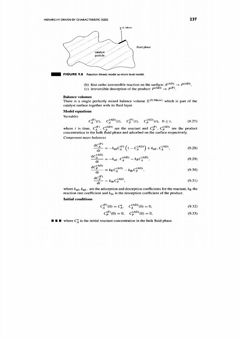
8/17/2019 Process Modelling and Model Analysis-Hangos-Cameron
http://slidepdf.com/reader/full/process-modelling-and-model-analysis-hangos-cameron 254/560
HIERARCHY DRIVEN BY CHARACTERISTIC SIZES
237
£ (S. Micro)
fluid phase
F I G U R E 9 . 8 Reaction kinetic model as micro level model.
(b) first-order irreversible reaction on the surface: A^^^^
-^
p(AD)^
(c) irreversible desorption of the produ ct: P^^^^ -> P^^\
Balance volumes
There
is a
single perfectly mixed balance volume x;(S.Micro) ^^jch
is
part
of
the
catalyst surface together w ith its fluid layer.
Model equations
Variables
-^(F),
^(AD),
-^(F),
^ (AD) .
-A'(^) '
^r^'if)^
C'p\t),
Cf'^'it),
0<f, (9.27)
where
t is
time,
C^\ C^^^ are the
reactant
and C^p\
C^^^^
are the
product
concentration in the bulk fluid phase and adsorbed on the surface respectively.
Component mass balances
dC
(F)
dC
dr
(AD)
= -;tadCf (l-C rO +^ ad -C ^'
AD)
dt
^ad-^^ I^RCJ ,
dc:
AD)
dt
dC]
= ^ RC^ ^ '''-)tdeCr^
dt
(F)
(9.28)
(9.29)
(9.30)
(9.31)
where kgd, ^ad - are the adsorption and desorption coefficients for the reactant, /CR the
reaction rate coefficient and k^ e is the desorption coefficient of the produc t.
Initial conditions
Ci''>(0)
=
cr'(O)
0,
where C^ is the initial reactant concentration in the bulk fluid phase.
(9.32)
(9.33)
8/17/2019 Process Modelling and Model Analysis-Hangos-Cameron
http://slidepdf.com/reader/full/process-modelling-and-model-analysis-hangos-cameron 255/560
238 CHAPTER 9 PROCESS MODEL HIERARCHIES
9.2.2. The Relation between Models of Different Levels Driven by
Characteristic Sizes
Modelling Goal and Modelling Assumptions
The modelling goal as well as the assumptions on the system boundaries and on the
input-output relations of the system and its environment are drastically and charac
teristically different on the various levels. The same applies for the assumptions on
the balance volumes.
Because the modelled process system is different on the various levels, the set
of modelling assumptions on the controlling mechanisms is also different. There is,
however, a relationship connecting models on various levels driven by characteristic
sizes seen also in their modelling assumptions. The modelling assumptions on a
lower level concern the detailed assum ptions on a particular subprocess or controlling
mechanism made at the higher levels.
Balance Volumes
Because the lower-level models driven by characteristic sizes are related to their
higher-level parent through z oom ing, the union of balance volumes of the same spatial
distribution at any level does not cover the union of that on a higher level. This can
be stated as
^ ( S . L o w e r ) ^ *
y 5,(S.Lower) ^ Q ^(S.Higher)^ ^^ 3^ ^
k=\ k=\
where
N^
^ ^x; *
•
Usually,
N^ = I
w hen we focus only on a particular single
balance volume at the lower-level and we build up a more detailed model of it as a
lower level model.
Variables and Model Equations
The above relation of the balance volumes gives a guideline on how the variables of
the higher and lower hierarchy level mo dels relate to each other. In the general case,
a higher level variable is obtained as some kind of average value of the lower level
variable of the same
kind.
This is averaged over the lower level balance volumes which
in turn constitute the higher level balance volume of the corresponding variable.
It is important to note, however, that only some of the variables and controlling
mechanisms of a higher level model are represented in a particular lower level model.
That is because different and even non-intersecting lower level models exist for a
given higher level model. In this case some of the higher level variables originate
from a lower level model and others are computed from another lower level model
by averaging.
Moreover, there is most often a relationship between the initial and boundary
conditions of the models of different levels driven by characteristic sizes.
EXAMPLE 9.2.3 (Relation between different level models driven by character
istic sizes of a simple packed bed tubular catalytic reactor). The (S.Mac ro) macro
hierarchy level model of the reactor is chosen to be the same as its (D.Bottom) bot
tom hierarchy level mod el described in Examp le
9.1.3.
The catalytic pellet mo del as a

8/17/2019 Process Modelling and Model Analysis-Hangos-Cameron
http://slidepdf.com/reader/full/process-modelling-and-model-analysis-hangos-cameron 256/560
HIERARCHY DRIVEN BY CHARACTERISTIC TIMES 239
(S.Meso) meso level model is shown in Example 9.2.1 and the surface kinetic model
as the (S.Micro) micro level model is in Example 9.2.2.
Balance volumes
We have the inclusion relation between the balance volumes of different hierarchy
levels driven by characteristic sizes:
v(5.Micro) ^
y^iSMezo) ^
v(^Bottom ) (9 35)
Moreover the micro level balance volume sC'^^icro)
^^ ^
y^^
^^^^ ^^
p ^ ^^ ^j^^
boundary surface for the meso level balance volume x;('^ ^^^so)
Model equations
Variahles
The micro level model variable (9.27) can be interpreted as the value of the meso
level variable (9.22) at the boundary, i.e.
Q ( 0 , 0 = c f \ (9.36)
Initial and boundary conditions
The overall reaction kinetic expression
kS^^^^^^C\
which appears in the boundary
condition (9.25) of the meso level component mass balance can be regarded as a
• I • solution of the micro level model for d Q /d r as its depends on its variable Q
.
9.2.3. Multi-scale Modelling and the Hierarchy Driven by Characteristic Sizes
Multi-scale modelling is an exciting and emerging field which covers modelling
aspects from the atomic to the continuum through the molecular and various meso-
scales. It includes but is not limited to such interesting and important topics as
surface reaction, formation of molecular and macromolecular aggregates, estimation
of mechanical properties of materials and fluid media at intermediate scales.
The work in mu lti-scale modelling is mainly performed in the area of solid-state
physics [59], physics of multi-phase systems [60], as well as multi-phase flows [61],
diffusion [62] and transport processes [63].
The set of models developed for multi-scale modelling can be arranged into a
hierarchy driven by characteristic sizes.
The micro level model of
this
hierarchy cor
responds to the molecular level multi-scale model, and the other models are arranged
according to the smallest species they take into account.
The model hierarchy driven by the level of detail for the simple packed bed
catalytic reactor described earlier in this section can be seen as a set of multi-level
models developed in the area of surface kinetics.
9.3. HIERARCHY DRIVEN BY CHARACTERISTIC TIMES
The relation between models of different hierarchy levels driven by characteristic
times is best understood if we imagine a detailed dynamic model. We can take a
model from the level (D.Bottom) or (D.Middle) with its full dynamics described as a
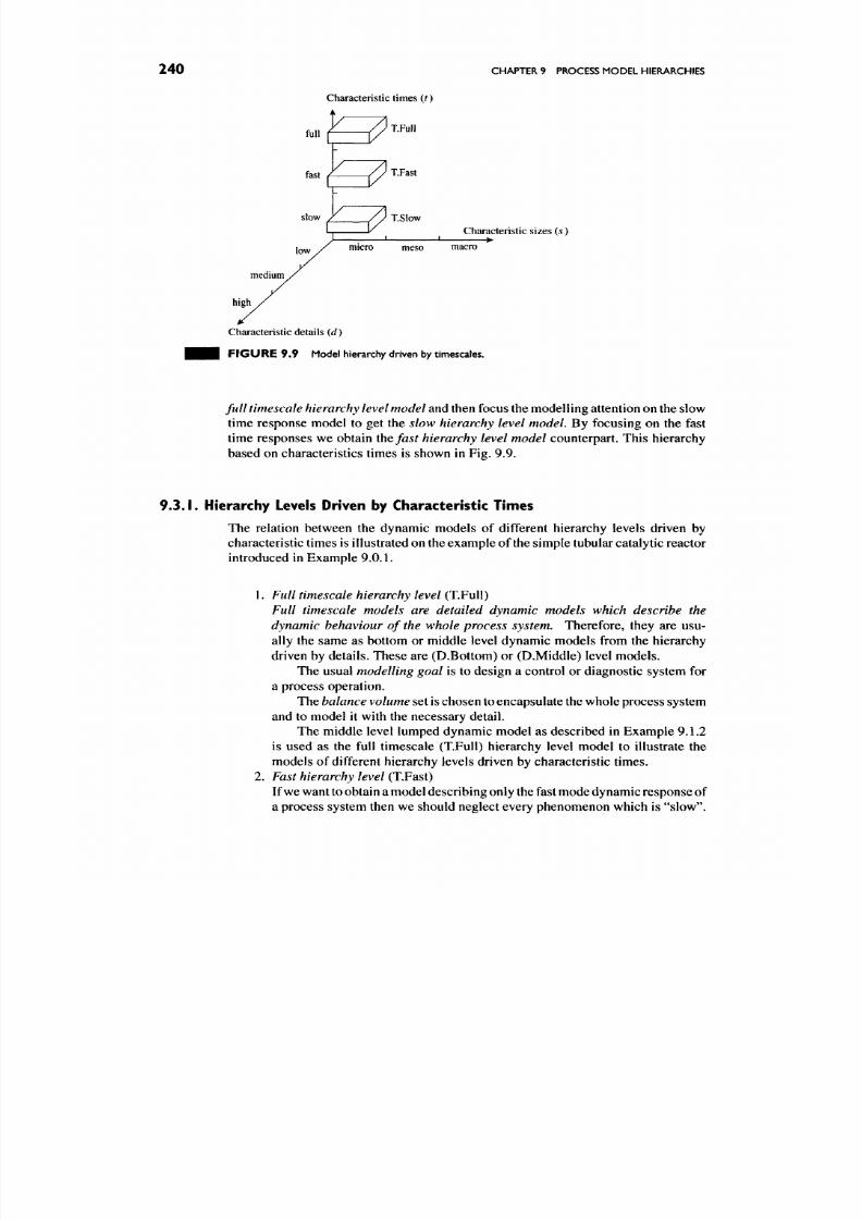
8/17/2019 Process Modelling and Model Analysis-Hangos-Cameron
http://slidepdf.com/reader/full/process-modelling-and-model-analysis-hangos-cameron 257/560
240 CHAPTER 9 PROCESS MODEL HIERARCHIES
Characteristic times (f)
f u ll - ^ / ' ™ »
fast
slow
T.Fast
_/ / T.Slow
medium
high /
low /
1 1
micro
meso
Characteristic sizes {s)
macro
Characteristic details {d)
F I G U R E 9 .9 Mode l hierarchy driven by timescales.
full timescale hierarchy level model and then focus the mod elling attention on the slow
time response model to get the slow hierarchy level model. By focusing on the fast
time responses we obtain
the fast hierarchy level model
counterpart. This hierarchy
based on characteristics times is shown in Fig. 9.9.
9 . 3 . 1 .
Hierarchy Levels Driven by Characteristic Times
The relation between the dynamic models of different hierarchy levels driven by
characteristic times is illustrated on the exam ple of the simple tubular catalytic reactor
introduced in Example 9.0.1.
1. Full timescale hierarchy level (T.FuU)
Full timescale models are detailed dynamic models which describe the
dynamic behaviour of the whole process system.
Therefore, they are usu
ally the same as bottom or middle level dynamic models from the hierarchy
driven by details. These are (D.Bottom) or (D.Middle) level models.
The usual modelling goal is to design a control or diagnostic system for
a process operation.
The balance volume set is chosen to encapsu late the whole process system
and to model it with the necessary detail.
The middle level lumped dynamic model as described in Example 9.1.2
is used as the full timescale (T.Full) hierarchy level model to illustrate the
mod els of different hierarchy levels driven by characteristic times.
2.
Fast hierarchy level
(T.Fast)
If we want
to
ob tain a model describing only the fast mode dynamic response
of
a process system then we should neglect every phenomenon which is "slow".
8/17/2019 Process Modelling and Model Analysis-Hangos-Cameron
http://slidepdf.com/reader/full/process-modelling-and-model-analysis-hangos-cameron 258/560

8/17/2019 Process Modelling and Model Analysis-Hangos-Cameron
http://slidepdf.com/reader/full/process-modelling-and-model-analysis-hangos-cameron 259/560
242
CHAPTER
9
PROCESS MODEL HIERARCHIES
where Q
(t )
and T^^^ are the reactant concentration and the temperature in the
kih
tank respectively and
t
is the time.
Component mass balances
^ = (cr -C«)-.„ ,9.40,
/: = 1,2 ,3,
d^\t) = dj^\t)
(9.41)
with
V
being the volume of the reactor,
F
is the flowrate, r^ the reaction rate and
C^^
is the inlet reactant concentration to the whole reactor.
Constitutive equations
Reaction rate equation
rA=h^-^I^^^^CA.
(9.42)
where ^o is the pre-exponential factor, E is the activation energy and R is the universal
gas constant.
Derived from static energy balances
0 = ^ ( r ( ' ^ - i ) - r ( * ) ) - ^ r ^ (9.43)
V ^ ^pep
)t=:
1 , 2 , 3 , r ^ O ) ^ j^(i)^ (9 44)
where
p
is the density,
cp
is the specific heat of the material in the reactor. A// the
reaction enthalpy and 7^*^ is the inlet temperature.
Initial conditions
C f
(0)
= q , ^ = 1 , 2 , 3 , (9.45)
where CJ is the initial concentration.
3. Slow hierarchy level
(T.Slow)
We can proceed in a similar fashion if we want to obtain a model describing
only the slow mode dynamic response of a process system. Here, we can
assume that the fast processes occur instantaneously. Interestingly enough it
is also done by imposing quasi steady-state assumptions in the form of
^ = 0 (9.46)
Qt
on dynamic variables
(p
but now with fast time variation compared with the
variation in other variables of the same model. The reason behind the quasi
steady-state assumption above is that the fast mode variable
(p
is regarded as
adjusting instantaneously to its new value.
It is important to remember again that "slow" and "fast" are relative
notions within a particular dynamic model because slow variations in one
model could well be fast in others.

8/17/2019 Process Modelling and Model Analysis-Hangos-Cameron
http://slidepdf.com/reader/full/process-modelling-and-model-analysis-hangos-cameron 260/560
HIERARCHY DRIVEN BY CHARACTERISTIC TIMES 243
The
balance volume
set is the same as for the full timescale level mode l.
Moreover
the set of
variables
is the
same
but
some
of the
differential vari
ables are transformed to algebraic variables due to the quasi steady-state
assumptions.
The concepts above
are
shown
on the
lumped middle level model
of
the
simple catalytic tubular reactor.
• • • EXAMPLE 9.3.2 (Slow respon se time mod el derived from the lumped m iddle
level model of a simple packed bed tubular catalytic reactor.)
Process system
Consider a plug flow tubular reactor com pletely filled with catalyst, and with a pseudo
first-order catalytic reaction A -> P exactly the same as for Example 9.1.2. The
flowsheet with
the
balance volumes
and
process variables
is
shown
in
Fig.
9.5.
Modelling goal
To describe the approximate
slow
dynamic input-output behaviour of the reactor for
design purposes.
Assumptions additional to the ones listed as 1-8:
A9. Neglect fast dynamics
in
component concentrations.
Balance volumes
We consider three balance volumes (i: |^ '^"'<"^), s fM idd le) ^^ ^(D.Middle)^ ^ j ^ ^
equal holdups
and
^ _ ^(D.Middle) I I (D.Middle) I I .(D.Middle) .g ^^.
Model equations
Variables
{Cf\
T^^Ht),
it = 1,2,3), 0<t, (9.48)
where Q and T^^\t) are the reactant c oncentration and the temperature in the ^th
tank, respectively
and
t
is the
time.
Energy balances
dt
V ^ ' pep
)k = 1, 2, 3, T^^'^ify = T^Ht) (9.50)
where p is the density, cp is the specific heat of the material in the reactor, AH the
heat
of
reaction,
V the
volume
of
the reactor,
F the
flowrate,
r^ the
reaction rate
and
T^^^ is the inlet reactant concentration to the whole reactor.
Constitutive equations
Reaction rate equation
rA=fcoe -^ /^^^^Q, (9 .51)

8/17/2019 Process Modelling and Model Analysis-Hangos-Cameron
http://slidepdf.com/reader/full/process-modelling-and-model-analysis-hangos-cameron 261/560
244
CHAPTER
9
PROCESS MODEL HIERARCHIES
where
ko
is the pre-exponential factor,
E
the activation energy, and
R
is the universal
gas constant.
Derived from static component mass b alances
^ - T i ^ t ' ' - C r ) - r A . (9.52)
A
= 1 , 2 , 3 ,
C^^\t) = C^^\t),
(9.53)
whe re Q is the inlet reactant conce ntration.
Initial conditions
r^^)(0) = r*, k= 1, 2,3 , (9.54)
I I I where T* is the initial tem perature.
9.3 .2. The Relation between Models of Different Levels Driven by
Characteristic Times
Modelling Goal and Modelling Assumptions
The modelling goal is usually related to control or diagnosis. The type of control or
diagnostic system considered affects the hierarchy level that is used for modelling.
Plant wide optimizing control usually needs slow hierarchy level models, whilst
regulation or on-line diagnosis needs fast ones.
The m odelling assum ptions not related to the timescale of the differential vari
ables are exactly the same for all levels including the assumptions on the system
boundaries and balance volumes.
Balance volumes
From the above, we can conclude that the balance volumes of all hierarchy levels
driven by characteristic times are exactly the same in spatial distribution and the
union of them encapsulates the whole process system. Hence, a
^ ( T . A n y )
E = U Ef^"y \ (9.55)
k={
Variables and Model Equations
The variables in models of all hierarchy levels driven by characteristic times are the
same by construction. However, some dynamic variables affected by quasi steady-
state assumptions in the fast or slow hierarchy level models, become algebraic
variables. Moreover, a dynamic variable transformed to an algebraic one by quasi
steady-state assumptions in the slow model should rem ain dynam ic in the fast model
and vice versa.
The initial (and boundary) conditions of the models at different levels driven
by characteristic times are exactly the same, except for the initial conditions of the
dynam ic balance equations affected by the fast or slow model assu mptions. Of co urse,
the variables set to algebraic ones lose their initial cond itions.

8/17/2019 Process Modelling and Model Analysis-Hangos-Cameron
http://slidepdf.com/reader/full/process-modelling-and-model-analysis-hangos-cameron 262/560
SUMMARY 2 4 5
• • • EXAMPLE 9.3.3 (Relationship b etween different level mod els driven by charac
teristic times of a simple packed bed tubular catalytic reactor.)
Balance volumes
They are exactly the same for the three models inherited from the middle level model
driven by detail:
5,(D.Middle)^ fe= 1,2,3.
Model equations
Variables
The variables are the same for models of all hierarchy levels driven by characteristic
times as defined in Eq. (9.4):
( c ^ ^ ^ O ,
T^^'Ht), ^ = 1,2,3), 0 < r ,
but Q , /: = 1, 2, 3 becom e algebraic variables in the slow hierarchy level model
and T^^\ k = 1, 2, 3 are algebraic variables in the fast one .
Balance equations
By the quasi steady-state assumptions generating the fast and slow models, we
transform the lumped dynamic energy balance to an algebraic set of equations
(Eqs.
(9.43)-(9.44)) in the fast model while the component mass balances of the
slow model becom e algebraic equations (9.52)-(9.5 3).
Initial conditions
The same or the corresponding initial conditions have been given to the dynamic
variables in the slow and fast hierarchy level models using the same initial values
• l i e * and r* .
The application of multi-time scale models to various process operations has
received significant attention. For example, Robertson and Cameron [64,65] used
spectral techniques to develop a family of models suitable for startup and shut
down problems in process systems. The models contained the appropriate timescale
behaviour for the application.
9.4. SUMMARY
This chapter has presented an overview of model hierarchies. The hierarchies were
based on three different but related views of the system being modelled. Inevitably
we must simplify our view of the system for modelling purposes. How we do that
can be in terms of detail of the balance volumes or the granularity of the model. We
can also look at characteristic sizes based on a macro, meso or micro view of the
phenomena occurring in the process. Finally, we can model our process based on
the characteristic dynamic modes. This leads to a hierarchy of process models which
contain various timescales of dynam ic behaviour from very fast to the slowest mod es.
The use of hierarchies is becoming an important aspect of modelling, driven by
the application area. The model we require for detailed design purposes can be quite
different from one used for control or for startup and shutdown studies. No one m odel
8/17/2019 Process Modelling and Model Analysis-Hangos-Cameron
http://slidepdf.com/reader/full/process-modelling-and-model-analysis-hangos-cameron 263/560
246
CHAPTER
9
PROCESS MODEL HIERARCHIES
will capture the necessary system attributes for all foreseeable applications. We need
models "fit for purpose".
9.5. FURTHER READING
Model hierarches are useful not only for establishing relationships between related
models but also for organizing safe and well-grounded information transfer between
them. There are rapidly developing fields within process systems engineering where
process model hierachies play a key role.
Multi-scale modelling
This field s driven by the basic science and engineering of materials, which are used in
electronic and optielectronic device fabrication. The related field in process systems
engineering has become a "challenge area" as reviewed by a recent paper in
AIChE
Journal [66]. Review papers in the field are also available, see e.g. [67,68].
9.6. REVIEW QUESTIONS
Q9.1. Describe the correspond ence between the
variables
of the models of the simple
packed bed tubular catalytic reactor (Example 9.0.1) of different hierarchy levels
driven by detail. (Section 9.1)
Q9.2. Describe the relation between the balance volumes of the models of the sim ple
packed bed tubular catalytic reactor (Example 9.0.1) of different hierarchy levels
driven by characteristic sizes. (Section 9.2)
Q9.3. Com pare the middle (D.M iddle) level model (see in Exam ple 9.1.2) and the
meso (S.Meso) level model (see in Example 9.2.1) of the simple packed bed tubular
catalytic reactor. What are the differences? Which one could be a sub-model of the
other? (Section 9.2)
Q9.4. Characterize the process systems appearing on the micro (S.Micro) level in the
hierarchy driven by ch aracteristic sizes. Give examples of the controlling mechan isms
you w ould describe on this level. (Section 9.2)
Q9.5. Characterize a potential full timescale (T.Full) level model in the hierarchy
driven by characteristic times. Which controlling mechanisms can be regarded
relatively slow and which ones relatively fast? (Section 9.3)
Q9.6.
Com pare the set of model equations in the full timescale (T.Full), fast (T.Fast)
and slow (T.Slow) level models in the hierarchy driven by characteristic times. How
does the number of dynamic balance equations vary with the level? (Section 9.3)
9.7. APPLICATION EXERCISES
A9.1.
Give the weighted average form of the relation of the middle and top level,
and that of the bottom and m iddle level mo dels driven by detail of the simple packed
bed tubular catalytic reactor introduced in Example 9.0.1. (Section 9.1)

8/17/2019 Process Modelling and Model Analysis-Hangos-Cameron
http://slidepdf.com/reader/full/process-modelling-and-model-analysis-hangos-cameron 264/560
APPLICATION EXERCISES
247
A9.2. Develop a meso (S.M eso) level model of a heat exchanger describing the heat
transfer through a metal wall. How would you use the modelling result on the macro
level describing the lumped model of a countercurrent heat exchanger consisting of
three lump pairs? (See Example 13.2.2 in Chapter 14) (Section 9.2)
A9.3.
Con sider a binary distillation column with 20 stages. Give the problem state
ment of modelling of its top, middle and bottom level models in the hierarchy driven
by detail. (Section 9.1)
A9.4,
Con sider a binary distillation column with 20 stages. Give the problem state
ment of modelling of its macro, meso and micro level models in the hierarchy driven
by characteristic sizes considering its middle (D.Middle) level model as its macro
level model. (Section 9.2)
A9.5. Con sider a comp lex process system familiar to you and try to develop and
describe the various model hierarchy levels driven by detail, driven by characteristic
sizes and driven by characteristic times.

8/17/2019 Process Modelling and Model Analysis-Hangos-Cameron
http://slidepdf.com/reader/full/process-modelling-and-model-analysis-hangos-cameron 265/560
This Page Intentionally Left Blank

8/17/2019 Process Modelling and Model Analysis-Hangos-Cameron
http://slidepdf.com/reader/full/process-modelling-and-model-analysis-hangos-cameron 266/560
PART II
ADVANCED PROCESS
MODELLING AND MODEL
ANALYSIS

8/17/2019 Process Modelling and Model Analysis-Hangos-Cameron
http://slidepdf.com/reader/full/process-modelling-and-model-analysis-hangos-cameron 267/560
This Page Intentionally Left Blank

8/17/2019 Process Modelling and Model Analysis-Hangos-Cameron
http://slidepdf.com/reader/full/process-modelling-and-model-analysis-hangos-cameron 268/560
BASIC TOOLS
FOR
PROCESS
MODEL ANALYSIS
This chapter is mainly devoted to the presentation of mathematical and computer
science background material which aids in the task of process model analysis. Con
cepts from systems and control theory such as nonlinear state space representations
(SSR s) and their linearized counterpa rts are extremely impo rtant as a starting point for
understanding the behaviour of models. The elementary notions behind these topics
are given in appendix A.
Section 10.5 is especially important because it contains the background material
for structural representation of nonlinear and linear dynamic state space equations
using structure matrices and graphs. These are powerful concepts which allow the
modeller to represent and analyze the model for a number of important characteris
tics which have direct influence on model behaviour in various applications such as
control.
10.1.
PROBLEM STATEMENTS AND SOLUTIONS
The analysis of process system models leads to mathematical problems of various
types. It is convenient and useful to formulate these mathematical problems in a
formal way specifying the inputs to the problem, the desired output or question to
be solved and indicate the procedure or method of solution. Such a formal problem
description can also be useful when we want to analyse the computational needs of a
mathematical problem or one of its solution methods.
251
8/17/2019 Process Modelling and Model Analysis-Hangos-Cameron
http://slidepdf.com/reader/full/process-modelling-and-model-analysis-hangos-cameron 269/560
252
CHAPTER
10
BASIC TOOLS FOR PROCESS MODEL ANALYSIS
The formal description of a mathematical problem will be given in a similar form
to algorithmic problem statements widely used in computer science [69]. According
to this formalism, p roblem statements have the following attributes:
• The title or name of the problem, with its optional abbreviation, e.g.
AVERAGING.
• The Given section where the input data of the problem are described.
• The
Question
to be answ ered or the output to be produced are specified under
the Find/Compute section.
• an optional
Method or Procedure
section describing the way of solving the
problem.
The following simple example of sam ple averaging illustrates the above concep ts.
• • i EXAMPLE 10.1.1 (Problem statement).
AVERAGING
Given:
A statistical sample of n elements, represented by a set of real numbers
{jci,
JC2,...
,Xn]
taken as measurements of independent equally distributed random
variables.
Compute:
The sample mean
jc,
where
1 ^
x= -Y^xi.
« , = i
Problem statements where
a
yes/no
Question
is to be answered
are
called
decision
problems, whilst problems with a Find/Compute section are termed
search
problems.
In the Method or Procedure section the key steps in solving the problem are
usually given in the form of a conceptual problem solution. The ingredients of a
conceptual problem solution are as follows:
1.
Solvability/feasibility^ analysis
Here w e answer the following key questions: D o we have a solution at all? If
yes,
is it unique?
2. Solution method (algorithm)
Here we set out the way in which the output is computed or the approach for
arriving at a d ecision.
3. Analysis of the problem and its solution method
Here we provide an analysis of how many com putational steps are needed for
solution and how this number of steps depends on the problem size.
The question of analysing the num ber of compu tational steps of a problem solu
tion and its dependence on the problem size is the subject of algorithmic complexity
theory within the theory of algorithms. The size of a problem is measured by the
number of digits or characters needed to describe an
instance
of the problem . This is
the set of problem ingredients specified in the Given section. There are fundamental
complexity c lasses which can be used to classify a particular problem . Problems with
polynomial dependence of their computational steps on their problem size belong
to the class
P
for decision problems or class
FP
for search problems. The problem

8/17/2019 Process Modelling and Model Analysis-Hangos-Cameron
http://slidepdf.com/reader/full/process-modelling-and-model-analysis-hangos-cameron 270/560
BASIC NOTIONS IN SYSTEMS AND CONTROL THEORY
253
classes
P
and
FP
are regarded to be computationally easy, w hile all the other problem
classes are computationally hard.
It is surprising but a fundamental fact in algorithmic complexity theory that the
problem class to which a particular problem belongs is not dependent on the solution
method but only on
the
problem statement itself
This is explained by the definition of
the computational steps needed to solve a problem. It is the largest number of steps
required to solve the problem for the worst possible
instance
of the problem using
the best available method.
10.2. BASIC NOTIONS IN SYSTEMS AND CONTROL THEORY
10.2.1. The Notion of a System, Linear and Time-Invariant Systems
A "sy stem " can be regarded as a basic notion in system theory. It is a general concept
under which a particular application can
be
classed. Such particular instances include a
"process system", a "financial system" or an "environmental system". We understand
the system to be part of the real world with a boundary between the system and its
environment. The system interacts with its environment only through its boundary.
The effects of the environment on the system are described by time dependent input
functions
u(t)
from a given set of possible inputs
u e U,
while the effect of the
system on its environment is described by the output functions y(t) taken from a set
of possible outputs
y ey.
The schematic
signal flow diagram
of a system S with its
input and output signals is shown in Fig. 10.1.
We can look at the signals belonging to a system as the input causing the time-
dependent behaviour of the system that we can observe through the output of the
system. Therefore, the system can be described as an operator S which maps inputs
u{t) into outputs y{t), expressed as
S:U->y, y = S[u].
For process control applications, we often distinguish between m anipulated input
variables
u(t)
and disturbance variables
d{t)
within the set of input variables to the sys
tem. Both manipu lated input and disturbance variables act upon the system to produce
the system behaviour. Disturbance variables are often regarded as uncontrolled being
determined by the environm ent in which the system resides. These disturbances could
be weather variations, process feed quality variations or variations in utility systems
M(0
inputs
system
states x(t)
y{t)
outputs
FIGURE 10 .1 Signal flow diagram of
a
system.

8/17/2019 Process Modelling and Model Analysis-Hangos-Cameron
http://slidepdf.com/reader/full/process-modelling-and-model-analysis-hangos-cameron 271/560
254
CHAPTER 10 BASIC TOO LS FOR PROCESS MO DEL ANALYSIS
such as Steam or cooling water tem peratures. In contrast, the manipulated input vari
ables can be directly affected by a controller or a person belonging to the environment
of the system.
There are systems with special properties which are especially interesting and
easy to handle from the viewpoint of their analysis and control. Here we investigate
a number of these systems.
Linear Systems
The first property of special interest is linearity. A system S is called
linear
if it
respond s to a linear comb ination of its possible input functions with the same linear
combination of the corresponding output functions. Thus, for the linear system we
note that
S[c\ui
+ C2U2]
= ciyi
+ C2J2 (10.1)
wi thci ,C2
eTl,ui,U2e
W,
j i , J2 ^ >'andS[Mi] =
J I , S [ M 2 ]
= ^ 2 -
Time-Invariant Systems
The second interesting class of systems are time-invariant systems. A system S is
time-invariant
if its response to a given input is invariant under time shifting. Loosely
speaking, time-invariant system s do not change their system prop erties in time. If we
were to repeat an experiment under the same circumstances at some later time, we
get the same response as originally observed.
The notion of time invariance is illustrated in Fig. 10.2, w here we see two identical
inputs to the system separated by a time Ar and note that the time shifted outputs
are also identical. In many process system applications, this can be a reasonable
assumption over a short time frame. In other cases, phenomena such as catalyst
deactivation or heat transfer fouling lead to non time-invariant system s. An in-depth
knowledge of the system me chanism s as well as the time frame of the intended analysis
often resolves the validity of the time-invariant assumption. There are a number of
implications which flow from the previous discussion.
Time-invariant systems have constant or time-independent parameters in their
system models.
Linear and time-invariant systems are termed LTI systems.
"(0
yit)
u{t)
fuit+At)
At
yit)
y{t+At)
At
FIGURE 10 .2 No tion of time invariance.
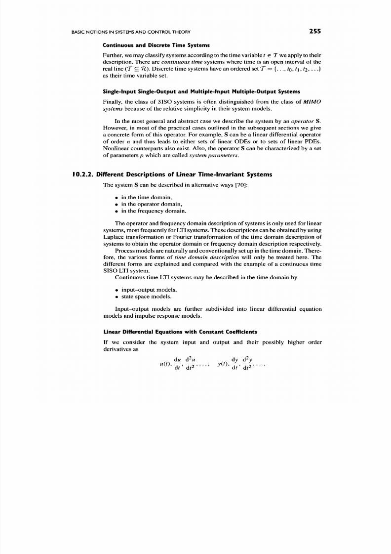
8/17/2019 Process Modelling and Model Analysis-Hangos-Cameron
http://slidepdf.com/reader/full/process-modelling-and-model-analysis-hangos-cameron 272/560
BASIC N OTIO NS IN SYSTEMS AND CONTROL THEORY 255
Continuous and Discrete Time Systems
Further, we may classify systems according
to the
time variable
r
€ T
we
apply
to
their
description. T here are
continuous time
systems where time is an open interval of the
real line ( T c
7Z).
Discrete time system s have an ordered
set T = {..., to
J\,t2^
--
•}
as their time variable set.
Single-Input Single-Output and Multiple-Input Multiple-Output Systems
Finally, the class of 5IS0 systems is often distinguished from the class of MIMO
systems
because of the relative simplicity in their system models.
In the most general and abstract case we describe the system by an operator S.
However, in most of the practical cases outlined in the subsequent sections we give
a concrete form of this operator. For example, S can be a linear differential operator
of order
n
and thus leads to either sets of linear ODEs or to sets of linear PDEs.
Nonlinear counterparts also exist. Also, the operator S can be characterized by a set
of parameters p which are called system parameters.
10.2.2.
Different Descriptions of Linear Time-Invariant Systems
The system S can be described in alternative ways [70]:
•
•
in the time domain,
in the operator domain,
in the frequency domain.
The operator and frequency d omain d escription of systems is only used for linear
system s, most frequently for LTI systems. These descriptions can b e obtained by using
Laplace transformation or Fourier transformation of the time domain description of
systems to obtain the operator domain or frequency domain description respectively.
Process m odels are naturally and conventionally set up in the time dom ain. Th ere
fore, the various forms of time domain description will only be treated here. The
different forms are explained and compared with the example of a continuous time
SISO LTI system.
Continuous time LTI systems may be described in the time domain by
• input-output models,
• state space mo dels.
Input-output models are further subdivided into linear differential equation
models and impulse response models.
Linear Differential Equations with Constant Coefficients
If we consider the system input and output and their possibly higher order
derivatives as
du d^u dy d^y

8/17/2019 Process Modelling and Model Analysis-Hangos-Cameron
http://slidepdf.com/reader/full/process-modelling-and-model-analysis-hangos-cameron 273/560
256 CHAPTER 10 BASIC TOO LS FOR PROCESS MO DE L ANALYSIS
F I G U R E 10 .3 Impulse response func tion.
the general form of the input-output model for an LTI SISO system is given by the
following higher order linear differential equation with constant coefficients:
d"j
( jn-U
dy dw d'H
This equation has the following initial conditions:
y(to) = yo.
d7
ytito).
i=
l , . . . , n .
Note that, in this case, the system parameters
p
consist of the set of constant
coefficients:
P = N . « , . . . ,
cifi,
bo , fci,..., brf. (10.3)
Impulse Response Representation
The impulse response function is the response of an LTI SISO system to a special test
input signal called the D irac delta function or unit impulse function. The Dirac delta
function
S(t)
is a function or more precisely a distribution in the mathematical sense,
which is equal to zero everywhere except at f = 0 such that
f
8(t)dt=\.
The concept of impulse response representation is illustrated in Fig. 10.3, where
h(t)
is the impulse response function and
8{t)
is the Dirac delta function.
The output of S can be written as
y(t)
-r
J-c
h{t
—
T)M(T)dr.
(10.4)
This equation describes the
convolution
of the functions
hi)
and
M()
in the time
domain. Here, /?(•) is the impulse response of the system and T is the variable of
integration.
8/17/2019 Process Modelling and Model Analysis-Hangos-Cameron
http://slidepdf.com/reader/full/process-modelling-and-model-analysis-hangos-cameron 274/560
BASIC NOTIONS IN SYSTEMS AN D CONTROL THEORY 257
Because w(r) is a function
IZ'^
->
1Z,
that is
u
maps from the set of positive real
numbers to the set of real numbers, we start the integration at time t = 0. The upper
bound for the integration is
t
because the system is
causal,
so that
= f h{t-
Jo
y(t)= / h{t-T)uiT)dT. (10.5)
Jo
Note that the
system parameters
of this representation are the parameters of the
impulse response function h{'). Impulse response functions can be parametrized or
represented by either the parameters of the input-output differential Eq. (10.3) or by
the parameters of the state space representation (SSR) so there is no need to specify
it as a function.
Unit Step Responses
The Dirac delta function used to gen erate the impu lse respon se from a system is physi
cally not realizable, nor even a function but a so-called distribution in the m athematical
sense. Therefore, one usually applies another special test function, the so-called unit
step function
to investigate the dynamic response characteristics of LTI systems.
The unit step function denoted by l(r ) is identically zero till = 0 where it jum ps
to 1 and remains identically 1 as r -> oo. The unit step function is the primitive
function of the Dirac impulse function:
\(t)=
/ (5( r)d r (10.6)
and has a discontinuity (a jump) at r = 0.
The response of a sy stem to the unit step function is called the unit step response
function.
The unit step response function /i*( 0
is the primitive function of the impulse
response function
f
Jo
h*(t)=
/
h(T)dT
(10.7)
because integration and the response generation of a LTI system are both linear
operations and thus commutative.
Note that a unit step response can be defined and generated experimentally for
every input-output pair of a MIMO LTI system to give a full characterization of its
multivariate dynamical responses.
It is impo rtant to note that a step response function will converge to a final value
hoQ in the limit (when
t
-> oo) if the impulse response function has a finite integral
in the limit. That is
poo
hoo= / hiT)dr < o o . (10.8)
Jo
This is exactly the condition for a LTI SISO system to be bounded input bounded
output (BIBO) stable (refer to Section 13.1.3). The value /IQO is called the
static
gain of the system. Note again that one can define static gains separately for every
input-output pair of a MIMO LTI system and arrange them into a matrix.

8/17/2019 Process Modelling and Model Analysis-Hangos-Cameron
http://slidepdf.com/reader/full/process-modelling-and-model-analysis-hangos-cameron 275/560
258 CHAPTER
10
BASIC TOO LS FOR PROCESS MODEL ANALYSIS
State Space Representation
Input-output representations describe
the
system with zero initial conditions. Given
the assumption of zero initial condition, we needed the impulse response function
h{t)
or its Laplace transform, the
transfer unction H{s),
a time instant
to
and the past
and future history of the input u(t),
0<T<to<t<ooio
compute y(t). Let us
introduce new information w hich is called the state of the system at
to
which contains
all past information on the system up to time to.
Now, to compute y(t)
for
t >to (all future values) we only need u(t), t >to and
the state at / = ^o-
The development
of a
state space model
of a
process system normally involves
identifying a number of classes of variables in the system. These include:
• state variable vector
x
elZ'^;
• (manipulable) input variable vector u e VJ' which is used to manipulate the
states;
• disturbance variable vector d elZ^;
• output variable vector y e 7^'" which is usually the measurements taken on
the system. These can be directly related to the states.
• system parameter vector/? e 1Z^,
It can be shown that the general form ofSSR or state space m odel of a MIMO
LTI system without considering disturbances separately from manipulated inputs
is
in the following form:
x{t)
= Ax(t) +
Bu(t), (state equa tion),
y{t) z=
CJC(0
+
DM( 0 ,
(output equation)
(10.9)
with given initial condition x(to) = x(0) and
x{t)
e TV\ y(t) e
TV^,
u{t) e W
(10.10)
being vectors of finite-dimensional spaces and
A € 7 ^ " ^ ^ B 6 7^'^^^ C € 7 ^ ' " ^ ^ DeT e '"^ '* (10.11)
being matrices. Note that A is called a state matrix, B is the input matrix, C is the
output matrix and D
is
the input-to-output coupling matrix.
The parameters of a state space model consist of the constant matrices
/7
=
{ A , B , C , D } .
The SSR of an LTI system is the quadruplet of the constant ma trices (A, B, C, D)
in Eq. (10.9).
The
dimension of an SSR is the dimension of the state vector: dim
x(t) =
n. The state space is the set of all states:
x(t)eX, dimA^
= n.
(10.12)
Simple Examples
of
LTI System Models
Some simple LTI system mod els are introduced in this subsection in order to illustrate
how to construct the canonical form (10.9) of their SSR and to show their step response
functions generated by MATLAB.

8/17/2019 Process Modelling and Model Analysis-Hangos-Cameron
http://slidepdf.com/reader/full/process-modelling-and-model-analysis-hangos-cameron 276/560
BASIC NO TIO NS
IN
SYSTEMS AND CONTROL THEORY
259
Having identified the state space realization matrices (A, B, C, D) of an LTI
system, there
is a
simple formula
to
compute
the
static gain
hoo of
the system from
the system parameters in the c ase of SISO systems:
ho o =
~CA-^B^D.
(10.13)
Note that the static gain related to an input-outpu t pair (ij) of a MIM O system can
also be computed
by a
similar extended version
of
the above formula:
hooiij)
= -C^'^«-^A-*B^'-'^ -h Df'-""\ (10.14)
where the upper index ^"^"^^ refers to theyth row, and ^ o* to the iih column of the
particular matrix.
• • i EXAMPLE 10.2.1
(A
simple stable SISO LTI system). Consider
a
simple LTI
SISO system model in the form:
djci
—i = - 4 J CI + 3 X 2 + 7MI, (10.15)
Qt
—± =
5JCI
- 6x2 +
8MI,
(10.16)
at
y
= xi.
(10.17)
1. Cons truct the state space model representation matrices.
2.
Com pute the unit step response function.
3. Com pute the static gain of the system.
The standard m atrix-vector form of the system m odel above is in the form of Eq. (10 .9)
with the following vectors and matrices
x=\
^J ,
u
= [uil y = ly],
C = [ 1 0 ], D = [0].
The unit step response is computed using the MATLAB procedure
s t e p (A, B , C , D)
to
obtain the step response shown
in
Fig.
10.4.
Note that the steady state gain is the asymptotic value of this function as time
goes
to
infinity.
The
static gain
can
also
be
computed separately from
the
formula
(10.13)
to
get 7.333
in
this case, w hich
is
also seen from the figure.
The next example shows
a
similar system extended with
a
new input variable
to
form a MISO model.
EXAMPLE 10.2.2 (A simple stable MISO LTI system). Consider a simple LTI
MISO model
in
the form:
djct
—i = -4JCI +3JC2 + 7MI, (10.18)
d^
dxo
— £
=
5x1
-
6x2
+
8M2,
(10.19)
at
y
= xi.
(10.20)

8/17/2019 Process Modelling and Model Analysis-Hangos-Cameron
http://slidepdf.com/reader/full/process-modelling-and-model-analysis-hangos-cameron 277/560
260
CHAPTER 10 BASIC TOO LS FOR PROCESS MO DEL ANALYSIS
Step Response
SISO System
F I G U R E 10.4 Un it step response for a stable SISO LTI system.
Construct the state space model representation matrices, compute the unit step
response function and com pute the static gain
of
the system.
Observe that the system above is almost the same as that in Example 10.2.1 but
a new input variable has been added.
The standard m atrix-vector form of the above system m odel is in the form of Eq. (10.9)
with the following vectors and matrices:
[1 M o-mi
-=["'i-
--
[0].
Observe, that both the vector u and also the input matrix B have changed.
The unit step response
is
again computed using M ATLAB
for
the input-output
pair (1, 1) to obtain the step respon se shown in Fig. 10 .5.
Note that the steady state gain
is
the asymptotic value
of
this function
as
time
goes to infinity. The static gain can also be computed separately from the multi input
multi output formula (10.14) to get 4.667 in this case which is also seen from the
figure.
The next example shows a MISO system with the same dimension of the system
variables and matrices but with the state matrix A changed. This example shows an
unstable system and illustrates how it can be discovered from the unit step response.
EXAMPLE 10.2.3
(An
unstable MISO
LTI
system). Consider
a
simple
LTI
MISO system model in the form:
lu\
(10.21)
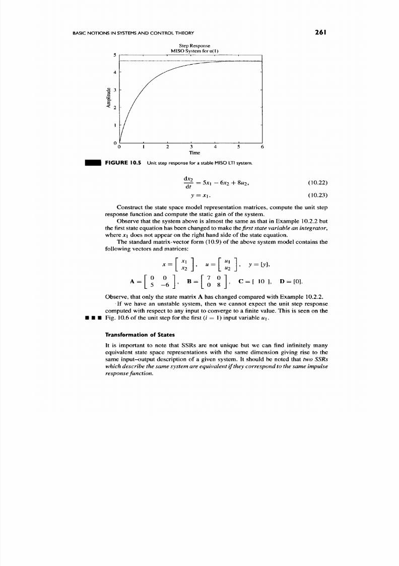
8/17/2019 Process Modelling and Model Analysis-Hangos-Cameron
http://slidepdf.com/reader/full/process-modelling-and-model-analysis-hangos-cameron 278/560
BASIC NOTIONS IN
SYSTEMS
AND CONTROL THEORY
261
Step
Response
MISO System for u( l)
F I G U R E 1 0 . 5 Un it step response fo r a stable MISO LTI system.
dx2 ^ ^ o
—— =
5X1
- 6 X 2 + 8 M 2 ,
at
(10.22)
(10.23)
Construct the state space model representation matrices, compute the unit step
response function and compute the static gain of the system.
Observe that the system above is almost the same as that in Example 10.2.2 but
the first state equation h as been changed to make the ^r^ r
state variable an integrator,
where x\ does not appear on the right hand side of the state equation.
The standard matrix-vector form (10.9) of the above system model contains the
following vectors and matrices:
[ 2 - . ] • - [ - ]
• • •
C = [ 10 ], D = [0].
Observe, that only the state matrix A has changed compared with Example 10.2.2.
If we have an unstable system, then we cannot expect the unit step response
computed with respect to any input to converge to a finite value. This is seen on the
Fig. 10.6 of the unit step for the first ( i = 1) input variable u\.
Transformation of States
It is important to note that SSRs are not unique but we can find infinitely many
equivalent state space representations with the same dimension giving rise to the
same input-output description of a given system. It should be noted that
two SSRs
which describe the same system are equivalent if they correspond
to
the same impulse
response function.
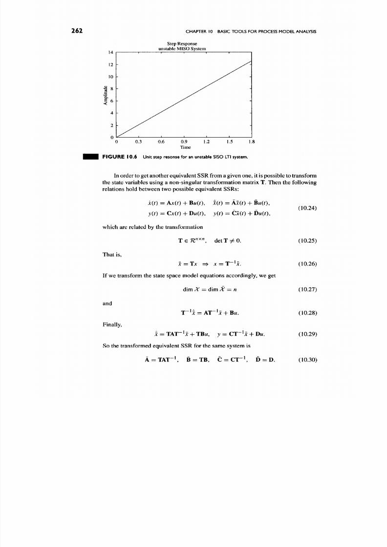
8/17/2019 Process Modelling and Model Analysis-Hangos-Cameron
http://slidepdf.com/reader/full/process-modelling-and-model-analysis-hangos-cameron 279/560
262
CHAPTER 10 BASIC TOO LS FOR PROCESS MO DEL ANALYSIS
14
12
10
| 8
| 6
4
2
Step Response
unstable MISO System
1 t 1 1 1 1
y ^
:
y ^
y ^
^—
1 1 1 1 1
0.3
0.6 0.9
Time
1.2
1.5
F I G U R E 10.6 Un it step resonse for an unstable SISO LTI system.
In order to get another equivalent SSR from a given one, it is possible to transform
the state variables using a non-singular transformation matrix T. Then the following
relations hold between two possible equivalent SSRs:
jc(0
= AJC(0 + B M ( 0 ,
X(S)
= AJc(0 + BM(0 ,
y(t)
= Cx(t) + DM(r), y(t) =
Cx{t)
+ DM(0,
which are related by the transformation
T e 7 ^ " ' " ' ,
d e t T ^ ^ O .
That is,
x
= Tx => x = T-^x.
If we transform the state space model equ ations accordingly, we get
dim A = d im ^ = n
and
Finally,
T~^^ = AT"^JC + BM.
X = TAT"^jc -h TBM, y = CT~^Jc
+
DM.
So the transformed equivalent SSR for the same system
is
A
=
TAT
^ B =
T B ,
C = CT ^ D = D.
(10.24)
(10.25)
(10.26)
(10.27)
(10.28)
(10.29)
(10.30)

8/17/2019 Process Modelling and Model Analysis-Hangos-Cameron
http://slidepdf.com/reader/full/process-modelling-and-model-analysis-hangos-cameron 280/560
BASIC N OTIO NS
IN
SYSTEMS AND CONTROL THEORY
263
State Space Models w ith Disturbance Variables
If the distinction between m anipulated v ariables u(t) and disturbance variables d(t) is
to be taken into accoun t then we consider an extended state space m odel form instead
ofEq. (10.9)as:
i ( 0 =
Ax{t)
+
Bu{t)
-f
Ed(t),
(state equ ation),
(10.31)
y(t) = Cjc(r) + Du{t) -h Frf(r), (output equation)
with given initial condition
x(to) =
jc(0), and an additional disturban ce variable
dit) e IV" (10.32)
with new state space matrices
E € 7^'^^^ F € 7e '"^ ^ (10.33)
Note that in this case the parameters of the state space models are
/7 = { A ,B ,C ,D ,E ,F } . (10.34)
Linear State Space Models w ith Time Varying Coefficients
The first step to generalize the state space models for LTI systems is to allow the
parameters to depend on time. It is important to note that the system described by
this extended state space model will no longer be time invariant. The resulting
linear
form with time varying coefficients is given by
djc(r)
— ^ = A(O x(0 + B(r)M(r) +
E{t)d{t),
(10.35)
d^
y{t) = C(t)x(t) -f D(t)u(t) -f- F ( 0 ^ ( 0 , (10.36)
where A(0 is an n x n state matrix, B(0 is an n x r input matrix, C(r) is an m x
n
output matrix,
D(t)
is an m x r input-to-output coupling matrix, E(0 is an n x v
disturbance input matrix and F(r) is an m x v disturbance output matrix.
1 0 . 2 3 . Nonlinear State Space Models
If the state of a nonlinear system can be described at any time instance by a finite-
dimens ional vector, then we call the system a concentrated parameter system. Process
systems described by lumped system models where the model is constructed from a
finite n umber of perfectly mixed balanc e volumes are concentrated parameter systems
from a system theoretical viewpoint.
Having identified the relevant input, output, state and disturbanc e variables for a
concentrated parameter nonlinear system, the general nonlinear state space equations
can be written in matrix form as
^=f(x(t),u(t),d(t),p),
(10.37)
at
y{t) = h(x{t),u(t),d(t),p). (10.38)

8/17/2019 Process Modelling and Model Analysis-Hangos-Cameron
http://slidepdf.com/reader/full/process-modelling-and-model-analysis-hangos-cameron 281/560
264
CHAPTER 10 BASIC TOOLS FOR PROCESS MODEL ANALYSIS
or in expanded form as
1
t
djC2
dXn
and
/ J l \
yi
f2ix\, . . . , X n , M i , ...,Ur,du ...,dv,p\, ...,pw)
V fn(Xi, ...,Xn,U\, ...,Ur,d\, . . . , r f v , P l , . . . , P w ) /
^ h\(x\,...,Xn,U\,...,Ur,d\,.,.,dv,p\,.,.,pw) \
h2(x\, . . ,,Xn, M l ,
...,Uf,d\, ,..,dv,p\,
. . . ,Pvv)
\ 3Vn / \ / ^ /„ ( xi , . . . , J f , i , M i , . . . , M r, ^ l , . • • » < ^ v , / ? l , - . M A V ) /
The nonlinear vector-vector functions/ and
h
in Eq. (10.38) characterize the
nonlinear system. Their parameters constitute the system parameters.
10.3.
LUMPED DYNAMIC MODELS AS DYNAMIC SYSTEM MODELS
The development of lumped dynamic models for process systems has been described
in detail in Section 5.2.
Lumped dynamic models are in the form of DAE systems where the
• differential equations originate from conservation balances of conserved
extensive quantities (mass, component masses, energy or momentum) for
every balance volume;
• algebraic equations are of mixed origin derived from constitutive relations.
These are normally no nlinear algebraic equations . They are often of full struc
tural rank indicating that the differential index of the DAE m odel is 1. Higher
index models result w hen this system is rank deficient.
Therefore, lumped dynamic models can be often transformed to set of explicit
first-order NL DEs w ith given initial cond itions. This form shows that lumped dy namic
models can be viewed as nonlinear state space models described in Section 10.2.3.
In this section, we show how the above elements of
a
lumped dynamic model of a
process system app ear in the nonlinear state space model. This correspondence gives
special properties to those nonlinear state space mod els which originate from lumped
dynamic models. These special properties can aid in the application of grey-box
methods for dynamic simulation and process control.
10.3.1. System Variables for Process Systems
In order to develop a state space model of a process system, we need to identify
the system variables. This includes the state, input, disturbance and output variables
of the system. For process systems these choices are dictated by the development
8/17/2019 Process Modelling and Model Analysis-Hangos-Cameron
http://slidepdf.com/reader/full/process-modelling-and-model-analysis-hangos-cameron 282/560
LUMPED DY NAM IC MODELS AS DYNA MIC SYSTEM MODELS 265
of the lumped parameter dynamic model of the process and by the setup of the
measurements and any control system. More precisely, state variables are fixed by
the lumped parameter dynam ic model while
inputy
disturbance and output variables
are fixed by the design, instrumentation and purpose of the model. We now consider
these variable categories.
State variables x{t)
The differential equations in a lumped dynamic model originate from conservation
balances for the conserved extensive quantities over each balanc e volum e. As the state
variables are the differential variables in these balance equations the natural set of
state variables of a process system is the set of conserved extensive variables or their
intensive counterparts for each balance volume. This fact fixes the number of state
variables. Hence, the dimension of the state space model is equal to the number of
conserved extensive quantities. If there are c com ponen ts in the system, then in general
we can w rite
c
component mass balances for each species plus an energy balance for
each phase. Thus, the total number of states n is obtained by multiplying the states
per phase {c
-\-
1) by the number of balance volumes n^'-n = {c + l)nx;. Moreover
the physical meaning of the state variables is also fixed by this correspondence.
Manipulated input and disturbance variables u{t), d{t)
In order to identify p otential input variables and disturbances one should look carefully
at the process to identify all dynam ic effects from the environmen t which act upon the
system to affect its behaviour. Those po tential input variables w hich can be influenced
by a device such as a control valve through an instrumentation system or changed
manually form the set of potential manipulated input variables. The actual purpose
of the modelling decides which variables will be regarded as actual disturbances and
manipulated input variables from the overall set. Typically, the following type of
signals are used as manipulated input variables in a process system:
• flowrates,
• split and recycle ratios,
• utility flowrates and tempe ratures,
• pressures,
• current and voltage controlling heaters, shaft rotation, motors or valves.
• switches.
Output variables, y{t)
The set of potential output variables is fixed by the measurement devices and each
measured variable can be regarded as an output of the system. The modelling or
control goal is the one which finally determines w hich variables are actually used for
a given purpose from the possible set. Typically, the following types of signals are
used as output variables in a process system:
• temperatures,
• pressures,
• conce ntration related physical quantities like mole or mass fraction,
• level related physical quantities like weight, head or total ma ss,
• flowrate related physical quantities.

8/17/2019 Process Modelling and Model Analysis-Hangos-Cameron
http://slidepdf.com/reader/full/process-modelling-and-model-analysis-hangos-cameron 283/560
266
CHAPTER
10
BASIC TOOLS FOR PROCESS MODEL ANALYSIS
10.3.2.
State Equations for Process System Models
Chapter 5 has considered in some detail the derivation of lumped parameter models
of process systems through the application of conservation principles.
In order to illustrate how the state equation of a nonlinear state space model
can be obtained from the lumped dynamic model of a process system consider the
following simple example.
• • • EXAMPLE 10.3.1 (Nonlinear state space model form of a CSTR model). Con
sider the nonlinear model describing the dynamics of a non-isothermal CSTR. The
reaction is first order,
A
—
> B
and is exothermic. The reaction rate constant
k
is
given by k{) Q-^I^^T^), The reactor
is
cooled by coolant at temperature 7c. The feed is
at temperature
T\.
It is assumed that the physical prop erties remain con stant and that
inlet and outlet flows are eq ual.
The mass and energy balances lead to the following equations:
y ^ = FCA,
-
FCA
-
kVCA, (10.39)
Vpcp^ = Fpcp(Ti -T) + kVCAi-AHR ) - UA{T - Tc)
at
(10.40)
with the volume
V
being constant.
These can be rearranged to give
d Q
dr
dT
lit
F
= y(^Ai -CA)-kCA,
F kCA
V pep
UA
Vpcp
(10.41)
( 7 - r c ) . (10.42)
Now the
state variables
of the nonlinear state space model of the CSTR are
x =
[CA,Tf,
which are in fact the intensive cou nterparts of the conserved extensive variables, these
being the mass of component A and the total energy E. L et us select the flowrate and
the coolant temperature as manipulated input variables:
u = [F, Tcf
Note that other choices for u are also possible.
Equations (10.41) and (10.42) are exactly the nonlinear state equations given in
(10.37) with n = 2 an d /i being the right-hand side function of the first an d/2 is that
of the second state equation.
10.3.3.
An Example of Constructing a Nonlinear State Space Model
from Lumped Dynamic Model
The following example illustrates how one can use an already developed lumped
dynamic process model in a systematic way to construct the nonlinear state space
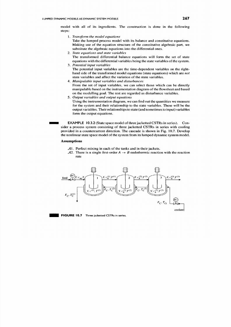
8/17/2019 Process Modelling and Model Analysis-Hangos-Cameron
http://slidepdf.com/reader/full/process-modelling-and-model-analysis-hangos-cameron 284/560
LUMPED DYNAMIC MODELS
AS
DYNAMIC
SYSTEM
MODELS
267
model with all of its ingredients. The construction is done in the following
Steps:
1.
Transform the model equations
Take the lumped process model with its balance and constitutive equations.
Making use of the equation structure of the constitutive algebraic part, we
substitute the algebraic equations into the differential ones .
2.
State equations and state variables
The transformed differential balance equations will form the set of state
equations with the differential variables being the state variables of the system.
3. Potential input variables
The potential input variables are the time-dependent variables on the right-
hand side of the transformed model equations (state equations) which are not
state variables and affect the variation of the state variables.
4. Manipulable input variables and disturbances
From the set of input variables, we can select those which can be directly
manipulable based on the instrumentation diagram of the flowsheet and based
on the modelling goal. The rest are regarded as disturbance variables.
5. Output variables and output equations
Using the instrumentation d iagram, w e can find out the quantities we m easure
for the system and their relationship to the state variables. These will be the
output variables. Their relationships to state (and sometimes to input) variables
form the output equations.
EXAMPLE 10.3.2 (State space model of three jacketted CST Rs in series). Con
sider a process system consisting of three jacketted CSTRs in series with cooling
provided in a countercurrent direction. The cascade is shown in Fig. 10.7. Develop
the nonlinear state space model of the system from its lumped dy namic system m odel.
Assumptions
^ 1 . Perfect mixing in each of the tanks and in their jack ets.
A2. There is a single first-order
A -> B
endothermic reaction with the reaction
rate
f
T (1 )
B
2 >|/^cf>,^(2)
f
T ( 3 )
^c ^c
3 >|/=:cf\r(3)
/^c.^ci
L-cJa^—1
coolant
F I G U R E 1 0 . 7 Three jacketted CSTRs in series.

8/17/2019 Process Modelling and Model Analysis-Hangos-Cameron
http://slidepdf.com/reader/full/process-modelling-and-model-analysis-hangos-cameron 285/560
268
CHAPTER 10 BASIC TOOLS FOR PROCESS MODEL ANALYSIS
rkmol l
rA = kCA J
Lsm^
J
in each of the tanks.
Ai.
The reaction rate coefficient
k
obeys Arrhenius law, i.e.
A4.
The volume of the mixture in the reactors and that in the cooling jacke ts is
constant.
^ 5 . The corresponding volum es and heat transfer area in the three CSTR s are
the same.
A6. Coun tercurrent flow of the reaction mixture and the cooling w ater.
Al.
The heat capacity of the wall is negligible.
^ 8 .
The physico-chem ical properties are constant.
Model equations
The dynamic model of the /th CSTR consists of the following balances:
•
Comp onent mass balance for component A in the reactor
V — ^
= FC^^~^^
- F& ^ - VC^^koQ-^l^'^, (10.43)
•
Energy balance of the reaction mixture
cppV—-
=
cppFT^'-^^
-
cppFT^^
at
- AHVC^^ho
e " ^ / ^ ^ +
KTA(T^^^
-
T^^).
(10.44)
•
Energy balance for the water in the jacket
cpcPcVc-^
=
cpcPcFcT^^^^
-
cpcPcFcT^c^
+KTA{T^^ - T^^^)
(10.45)
for every CSTR, i.e. for / = 1, 2, 3.
The following "boundary conditions" specify the inlet and the outlet conditions
for the reaction mixture and the cooling water respectively:
d^ ^
= Q . ,
T^^^
=
Tu
T^c^ =
TQ.
(10.46)
Moreover, we need proper initial conditions for every differential variable at time
t = 0
C^'^(O),
T^'HO), T^\0),
i = 1,2, 3.
State variables and state equations
The state variables of the system consisting of the three jacketted CSTRs are dictated
by the balance equations to be
x=\d \T '\Tl^
\i=\,2,3\ .
(10.47)
8/17/2019 Process Modelling and Model Analysis-Hangos-Cameron
http://slidepdf.com/reader/full/process-modelling-and-model-analysis-hangos-cameron 286/560
8/17/2019 Process Modelling and Model Analysis-Hangos-Cameron
http://slidepdf.com/reader/full/process-modelling-and-model-analysis-hangos-cameron 287/560
270
CHAPTER 10 BASIC TOOLS FOR PROCESS MODEL ANALYSIS
^ i ^ EXAMPLE 10.4.2 (Sim ple linea r exam ple). In contrast to the previous example,
the equation describing the dynamics of a temperature sensor is given by
AT 1
^ =
-(T-Ts).
(10.51)
dr r
• • • This is linear in Ts.
Having the linearized equations has several advantages including:
• The super-position theory applies. This means that if jci and X2 are solutions
of the model then so too are jcj + X2 or c x\ or CJC2.
• There is a wealth of powerful and readily available analysis tools, e.g. in
MATLAB and Mathematica.
• The initial conditions in the ODEs are zero when the equations are written in
terms of deviation variables.
• Changes in outputs are in direct relationship to input chang es. If a change of
AM in the input gives rise to a change of
Ay
in the output, then 2 AM will lead
to an output change of 2 Aj.
In the following paragraphs, we describe how linearization is done.
Linearization of equations can b e applied to both algebraic and differential equa
tions. Linearization can be done at any convenient point in the state space but is
usually done at some steady-state point of the system.
It is often the case in control applications that we want to work with deviation
(perturbation) variables
which are defined in relation to a reference point or steady-
state operating point. Thus , the deviation variable
x
can be defined as
JC
= Jc -x o , (10.52)
where
XQ
is the particular steady-state value of x. We can also use a normalized form
as
X =
(10.53)
to ensure that we have provided some scaling to the problem. These variables, x are
then "deviations" from a particular steady-state value, XQ.
Linearization is based on the application of Taylor's expansion about a particular
operating point. For the general dynamic model in one variable, x we can write:
^ = / ( ^ , 0 (10.54)
Qt
and the expansion of the nonlinear function/(jc, 0 gives
+ • • • , (10.55)
( j c , 0 = / ( J c o , 0 + ^
ox
(X - - O) + T-y
(X-XO)^
2
•^0
where
XQ
is the operating point and d'//d jc' is the
iih
derivative
off
with respect to
x
evaluated at
^0-
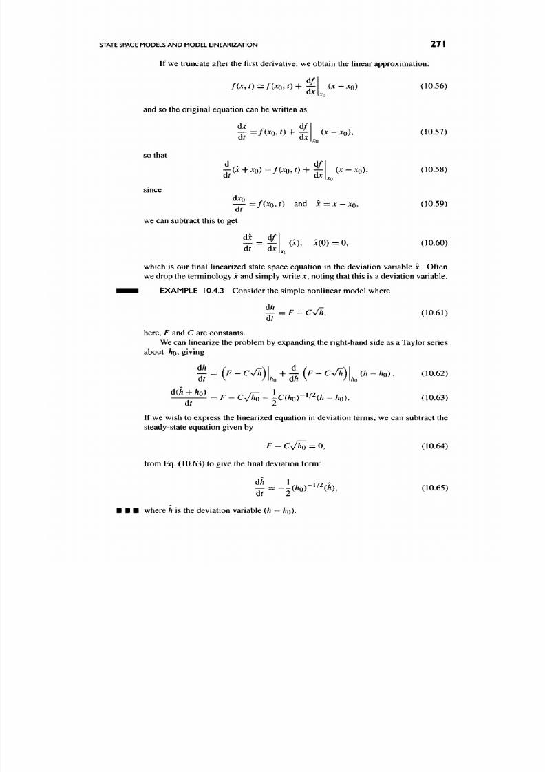
8/17/2019 Process Modelling and Model Analysis-Hangos-Cameron
http://slidepdf.com/reader/full/process-modelling-and-model-analysis-hangos-cameron 288/560
STATE SPACE MODELS AN D MOD EL LINEARIZA TION
271
If we truncate after the first derivative, we obtain the linear approxim ation
d /
f{xJ)c:^f{xoJ) +
dx
(x - xo)
XQ
and so the original equation can be written as
dx , d/
(X-Xo),
XQ
SO that
since
d .
df
-(x-\-xo)=f{xoJ)-^ -j-
dt dx
( ^ - xo ) ,
xo
dxo
dt
-fixoyt) and x=x— xo,
we can subtract this to get
dx_^
dt dx
(x);
x(0) =
0,
(10.56)
(10.57)
(10.58)
(10.59)
(10.60)
XQ
which is our final linearized state space equation in the deviation variable Jc. Often
we drop the terminology Jc and simply write JC , noting that this is a deviation variable.
EXAMPLE
10.4.3
Consider the simple nonlinear mo del where
dh
dt
F-CVh,
(10.61)
here, F and C are constants.
We can linearize the problem by exp anding the right-hand side as a Taylor series
about
ho ,
giving
dh
'dt
= (F- cVh)I + ^ ( F - cVh)I
(h
- ho), (10.62)
V
/\ho dh \ /\ho
^A+ M = F.cVh-o-\cihor^^hh-ho).
(10.63)
If we wish to express the linearized equation in deviation terms, we can subtract the
steady-state equation given by
F - Cy/h^ = 0,
from Eq. (10.63 ) to give the final deviation form:
^ = -i(.o)-"^<« .
(10.64)
(10.65)
where
h
is the deviation variable
(h
—
H Q ) .

8/17/2019 Process Modelling and Model Analysis-Hangos-Cameron
http://slidepdf.com/reader/full/process-modelling-and-model-analysis-hangos-cameron 289/560
272
CHAPTER 10 BASIC TOOLS FOR PROCESS MOD EL ANALYSIS
In general, it can be seen that for a single variable non linear expression given by
(10.66)
x
the linearized equation is
dx d ^
d7 = d7^"-^«^
-{i)-'^-^^'-{iy
'''•'''
If there are any accompanying output equations y(t) — h(x(t),
u(t)),
then these
are also linearized and represented in deviation form as
where the partial derivatives are evaluated at the chosen operating point.
(10.68)
10.4.2. Multi-variable Linearization
We can extend the single variable linearization to the case where we have many
variables in our model. Hence, consider the set of ODEs given by
or
dx
— - =MxuX2,X3,. . . ,Xn),
at
-JT =f2(x\,X2,X3,.,.,Xn).
at
(10.69)
(10.70)
- 7 -
=M^\^X2.X3,,,. ,Xn).
at
Linearization m eans expanding the right-hand sides as a multi-variable Taylor series.
Consider the first equation in (10.69) which can be expanded about the point
(^lo '-^2o»- '-^no)togive:
at dx[
(x \ -•^io) + --- +
-^In
dXn
{Xfi — Xfif)
)
(10.71)
'"0
(^j ^jo)'
If we do this for all equations ( 1 , . . . , n) we obtain
\Xj Xjo)i i = 1, . . ., W.
dt
(10.72)
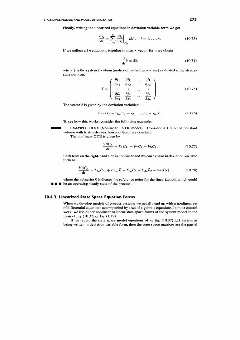
8/17/2019 Process Modelling and Model Analysis-Hangos-Cameron
http://slidepdf.com/reader/full/process-modelling-and-model-analysis-hangos-cameron 290/560
STATE SPACE MODELS AN D MODEL LINEARIZA TION
273
Finally, writing the linearized equations in deviation variable form we get
dr f-f dxj
(xi),
i= 1,
...,n.
(10.73)
If we collect all n equations together in matrix-vector form we obtain
d
dt
(10.74)
where J is the system Jacob ian (m atrix of partial derivatives) evaluated at the steady-
state point XQ.
dx\ dX2 dXn
5 =
\ dx\ dX2 dXn /
(10.75)
The vector jc is given by the deviation variables:
•^ T
X = (Xi —
X J Q ,
X2 — XjQi . . . jXfi — XHQ ) .
To see how this works, consider the following example:
(10.76)
EXAMPLE 10.4.4 (Nonlinear CSTR m odel). Con sider a CSTR of constant
volume with first-order reaction and fixed rate con stant.
The nonlinear OD E is given by
dt
FICA. -F2CA-VkCA.
(10.77)
Each term on the right-hand side is nonlinear and we can expand in deviation v ariable
form as
VdCA
dt
F\OCAI +
CA^^F - F2^CA - CAoh - VKCA),
(10.78)
where the subscript 0 indicates the reference point for the linearization, which could
be an operating steady state of the process.
10.4.3. Linearized State Space Equation Forms
When we develop models of process systems w e usually end up w ith a nonlinear set
of differential equation s accom panied by a set of algebraic equation s. In most control
work, we use either nonlinear or linear state space forms of the system model in the
form of
Eq.
(10.37) or Eq. (10.9).
If we regard the state space model equations of an Eq. (10.37) LTI system as
being written in deviation variable form, then the state space matrices are the partial
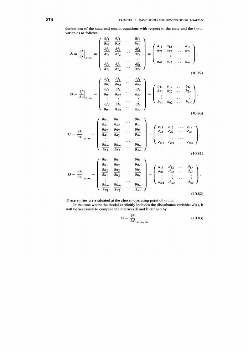
8/17/2019 Process Modelling and Model Analysis-Hangos-Cameron
http://slidepdf.com/reader/full/process-modelling-and-model-analysis-hangos-cameron 291/560

8/17/2019 Process Modelling and Model Analysis-Hangos-Cameron
http://slidepdf.com/reader/full/process-modelling-and-model-analysis-hangos-cameron 292/560
STATE SPACE MODELS AN D MODEL LINEARIZA TION 275
and
(10.84)
= —
dd
xoatoJo
EXAMPLE 10.4.5 (Linearization
of a
CSTR model). Consider
the
nonlinear
model describing the dynamics of a non-isothermal C STR. The reaction is first order,
A —> B and is exothermic. The reaction rate constant k is given by fcoe~^/^^^\
The reactor is cooled by coolant at temperature
TQ,
It is assumed that the physical
properties remain constant and that inlet and outlet flows are equal.
The mass and energy balances lead to the following e quation s:
V ^ = FCA, - FCA - kVCA, (10.85)
Vpcp^
=
Fpcp(Ti
- D +
kVCA(-AHK)
-
UA(T
- Tc). (10.86)
at
These can be rearranged to give
dCA F
- I T = TA^A: -
CA)
- kCA. (10.87)
Qt V
dT F kCA UA
— = -(Ti - D + - A ( _ A / / R ) - {T - Tc ). (10.88)
dr
V pep
ypcp
Now we linearize the equations above in the following steps:
•
First,
we can classify the variables within the nonlinear state space formulation
as
x = [CA.Tf, y = [CA,Tf, u = [F,Tcf;
other choices
for u
are possible.
•
Second,
convert the original nonlinear ODEs into linear state space form.
The partial derivatives with respect to the states x are given by
- ^ == I -{CA - CA ) I
ikCA)
(10.89)
dxx dCA\y
) dCA
dfx
d /F \ d
^ = ^ ( ^ ( Q , - Q ) ) - - ( . Q ) (10.91)
= - ^ o ( ^ ) e - ^ / ( « ^ o ) c , „ . (10.92)

8/17/2019 Process Modelling and Model Analysis-Hangos-Cameron
http://slidepdf.com/reader/full/process-modelling-and-model-analysis-hangos-cameron 293/560
27 6
CHAPTER 10 BASIC TOOLS FOR PROCESS MODEL ANALYSIS
= —(-AHR)
(10.95)
pep
- (- A //R ), (10.96)
pep
( ^ — )
( i ^ ^ ^ - ^ ^ > ' '''•'''
-E/(R7-o)c^^(z^«R) _ ^ (10.99)
A
pep Vpep
The partial derivatives with respect to the inputs
u
are
= { iC,,-CA))- ikC,) (10.100)
9MI
_ (Q j
-
CAQ)
(Ti
-
T)
UA
Vpep.
(10.101)
( ^ ( Q i - CA))
-
(kCA) (10.102)
V
du 2
97c
= 0, (10.103)
- ^ ( i ^ < ' ' - ^ = > l " « •" " >
(10.106)
(10.109)
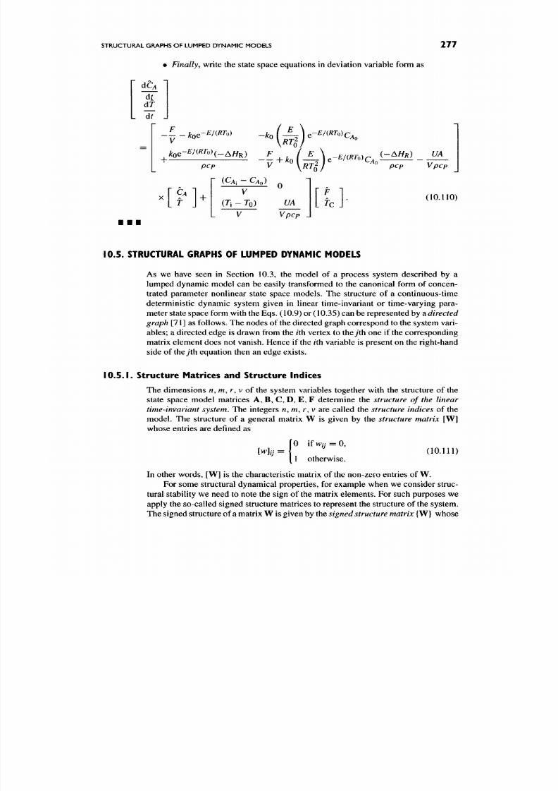
8/17/2019 Process Modelling and Model Analysis-Hangos-Cameron
http://slidepdf.com/reader/full/process-modelling-and-model-analysis-hangos-cameron 294/560
STRUCTURAL GRAPHS OF LUMPED DYNAMIC MODELS 277
• Finally, write the state space equations in deviation va riable form as
d Q
dT
It J
pep V \RT^I pep
(-AHR) UA
Vpcp
m
( Q . -
CAQ)
V
(Ti - To) UA
Vpcp J
[y-
(10.110)
10.5.
STRUCTURAL GRAPHS OF LUMPED DYNAMIC MODELS
As we have seen in Section 10.3, the model of a process system described by a
lumped dynamic model can be easily transformed to the canonical form of concen
trated parameter nonlinear state space models. The structure of a continuous-time
deterministic dynamic system given in linear time-invariant or time-varying para
meter state space form w ith the Eqs. (10.9) or (10.35) can be represented by a directed
graph
[71] as follows. T he nodes of
the
directed graph correspond to the system vari
ables; a directed edge is drawn from the
ith
vertex to theyth one if the corresponding
matrix element does not vanish. Hence if the iih variable is present on the right-hand
side of theyth equation then an edge exists.
10.5.1. Structure Matrices and Structure Indices
The dimensions n, m, r, v of the system variables together with the structure of the
state space model matrices A, B, C, D, E, F determine the structure of the linear
time-invariant system.
The integers n, m, r, v are called the
structure indices
of the
model. The structure of a general matrix W is given by the structure matrix [W]
whose entries are defined as
Mij
0 i f w y = 0 ,
1 otherwise.
(10.111)
In other word s, [ W ] is the characteristic matrix of the non-zero entries of W .
For some structural dynamical properties, for example when we consider struc
tural stability we need to note the sign of the matrix elements. For such purposes we
apply the so-called signed structure matrices to represent the structure of the system.
The signed structure of a matrix W is given by the signed structure ma trix {W} whose
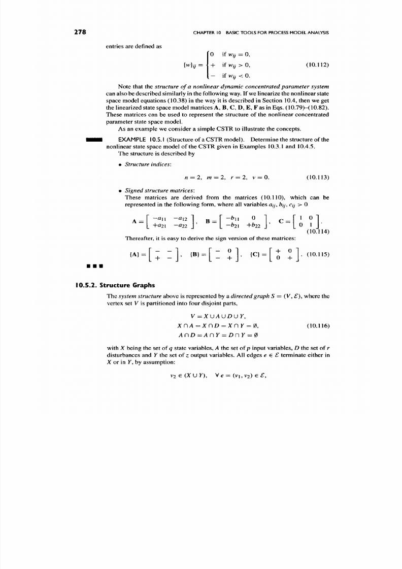
8/17/2019 Process Modelling and Model Analysis-Hangos-Cameron
http://slidepdf.com/reader/full/process-modelling-and-model-analysis-hangos-cameron 295/560
278
CHAPTER
10
BASIC TOOLS
FOR
PROCESS MODEL ANALYSIS
entries are defined as
0 if Wij
=
0,
+
if
Wij
>0,
(10.112)
— if Wij < 0.
Note that the
structure of
a
nonlinear dynamic concentrated parameter system
can also be described similarly in the following way. If we linearize the nonlinear state
space mod el equations (10.38) in the way it is described in Section 10.4, then we get
the linearized state space model matrices A, B , C, D , E, F as in Eqs. (10.79)-(10.82).
These matrices can be used to represent the structure of the nonlinear concentrated
parameter state space model.
As an example we consider a simple CSTR to illustrate the concepts.
EXAMPLE 10.5.1 (St ruc ture of a CSTR mod el). Determine the structure of the
nonlinear state space model of the CSTR given in Examp les 10.3.1 and 10.4.5.
The structure is described by
•
Structure indices:
n = 2, m = 2, r = 2, v = 0. (10.113)
• Signed structure matrices:
These matrices are derived from the matrices (10.110), which can be
represented in the following form, wh ere all variables aij, bij,
Cij
> 0
\ -an -an]
^ . f - ^ i i 0 1 r - T ^ ^ 1
^ - [
+a2i
-a22 J ' L -^21 +^22 J ' [0 1 J •
(10.114)
Thereafter, it is easy to derive the sign version of these matrices:
{ A } = [ 7 " 1 , { B } = r ~ ^ 1 , { C } = r j ^ 1 . (1 0. 11 5)
• • •
10.5.2. Structure Graphs
The
system structure
above is represented by a
directed graph S =
(V, f ) , w here the
vertex set V is partitioned into four disjoint parts,
V
=XUAUDUY,
xnA
=
xnD
=
xnY = 0,
(10.116)
Ar\D =
AnY
=
Dr\Y =
id
with
X
being the set of ^ state variables,
A
the set of p input variables,
D
the set of
r
disturbances and Y the set of z output variables. All edges e e £ terminate either in
X or in F, by assumption:
V 2 G ( X U F ) , V ^ = ( v i , V 2 ) € £ : ,
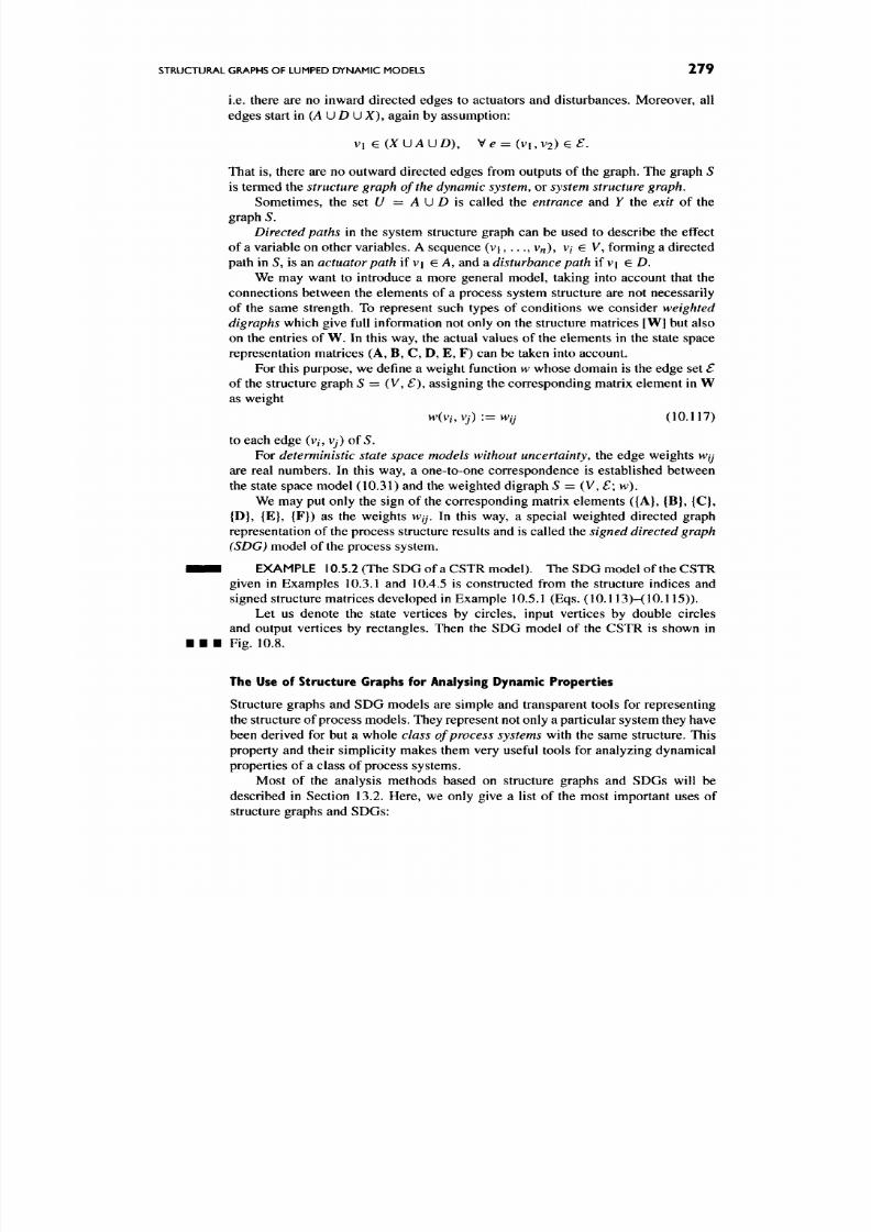
8/17/2019 Process Modelling and Model Analysis-Hangos-Cameron
http://slidepdf.com/reader/full/process-modelling-and-model-analysis-hangos-cameron 296/560
STRUCTURAL GRAPHS OF LUMPED DY NAMIC MODELS 279
i.e. there are no inward directed edges to actuators and disturbances. Moreover, all
edges start in (A U D U X ), again by assum ption:
VI
e (XUAUD ), We = (vuv2) e£.
That is, there are no outward directed edges from outputs of the graph. The graph 5
is termed the
structure graph of the dynamic system,
or
system structure graph.
Som etimes, the set [/ = A U D is called the entrance and Y the exit of the
graph 5.
Directed paths
in the system structure graph can be used to describe the effect
of a variable on other variables. A sequence (vi,..., v„), v, e V, forming a directed
path in 5, is an
actuator path
if vi G A, and a
disturbance path
if vi
e D.
We may want to introduce a more general model, taking into account that the
connections between the elements of a process system structure are not necessarily
of the same strength. To represent such types of conditions we consider
weighted
digraphs which give full information not only on the structure matrices [W] but also
on the entries of W. In this way, the actual values of the elements in the state space
representation matrices (A, B , C, D, E, F ) can be taken into account.
For this purpose, we define a weight function
w
whose domain is the edge set
£
of the structure graph S = (V , £ ), assigning the corresponding matrix element in W
as weight
w(v/,v/) :=Wij (10.117)
to each edge (v/, vy) of 5.
For deterministic state space models without uncertainty, the edge weights w/y
are real numbers. In this way, a one-to-one correspondence is established between
the state space model (10.31) and the weighted digraph S = (V , S; w).
We may put only the sign of the corresponding matrix elements ({A}, {B}, {C},
{D}, {E}, {F}) as the weights w/y. In this way, a special weighted directed graph
representation of the process structure results and is called the
signed directed graph
(SDG) model of the process system.
• i ^ EXAMPLE 10.5.2 (The SDG of a CSTR mo del). The SDG model of the CSTR
given in Examples 10.3.1 and 10.4.5 is constructed from the structure indices and
signed structure matrices developed in Example 10.5.1 (Eqs. (10.113)-(1 0.115)).
Let us denote the state vertices by circles, input vertices by double circles
and output vertices by rectangles. Then the SDG model of the CSTR is shown in
• • • Fig. 10.8.
The Use of Structure Graphs for Analysing Dynamic Properties
Structure graphs and SDG models are simple and transparent tools for representing
the structure of process mo dels. They represent n ot only a particular system they have
been derived for but a whole class of process systems with the same structure. This
property and their simplicity makes them very useful tools for analyzing dynamical
properties of a class of process systems.
Most of the analysis methods based on structure graphs and SDGs will be
described in Section 13.2. Here, we only give a list of the most important uses of
structure graphs and SD Gs:
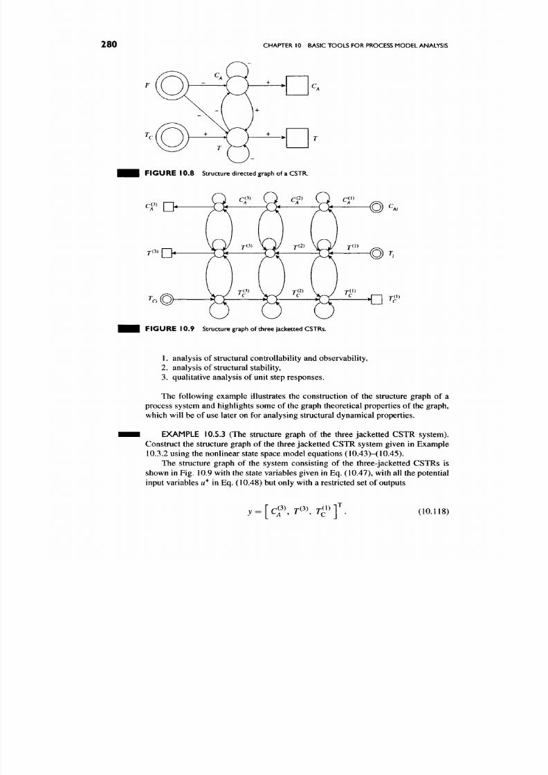
8/17/2019 Process Modelling and Model Analysis-Hangos-Cameron
http://slidepdf.com/reader/full/process-modelling-and-model-analysis-hangos-cameron 297/560
280
CHAPTER 10 BASIC TOOLS FOR PROCESS MODEL ANALYSIS
+
F I G U R E 1 0 . 8 Structure directed graph of
a
CSTR.
^^ D
TO)
Q
FIGURE 10 .9 Structure graph of three jacketted CSTRs.
1. analysis of structural controllability and observability,
2. analysis of structural stability,
3. qualitative analysis of unit step respon ses.
The following example illustrates the construction of the structure graph of a
process system and highlights some of the graph theoretical properties of the graph,
which will be of use later on for analysing structural dynamical properties.
EXAMPLE 10.5.3 (The struc ture graph of the three jack etted C STR system) .
Construct the structure graph of the three jacketted CSTR system given in Example
10.3.2 using the nonlinear state space model equations (10.43)~(10.45).
The structure graph of the system consisting of the three-jacketted CSTRs is
shown in Fig. 10.9 with the state variables given in Eq. (10.47 ), with all the potential
input variables M* in Eq. (10 .48) but only w ith a restricted set of outputs
j = [ c f , r(3), r^')]'
(10.118)

8/17/2019 Process Modelling and Model Analysis-Hangos-Cameron
http://slidepdf.com/reader/full/process-modelling-and-model-analysis-hangos-cameron 298/560

8/17/2019 Process Modelling and Model Analysis-Hangos-Cameron
http://slidepdf.com/reader/full/process-modelling-and-model-analysis-hangos-cameron 299/560
282
CHAPTER 10 BASIC TOOLS FOR PROCESS MODEL ANALYSIS
Q10.8. Describe why linearization of the nonlinear state space model is often useful
in model analysis and application. What role do deviation or perturbation variables
play in this form of the m odel? (Section 10.4)
Q10.9.
Describe several types of structural graphs of nonlinear and linear state space
models. What are the principal characteristics of these graphs and how can they be
used for further analysis of a process system? (Section 10.5)
10.8. APPLICATION EXERCISES
AlO.l . Consider the simple nonlinear model where
dh r-
— =F-C4h, (10.119)
df
Here F and C are constants. Linearize the model and compare the original non
linear equation (10.119) with the linearized form of equation to observe the effect of
linearization and the error involved as we move further away from the linearization
point /?o- To do this, solve both models in MATLAB and observe what happens with
the deviation of the linear model as h increases. Use values of F = 0.5 and C = 0.75
with /z(0) = 0.1. Comment on the results. (Section 10.4)
A10.2. Linearize the Arrhenius reaction rate term given by
jt
=
jtoe-^/^^ ^> (10.120)
(Section 10.4)
A 10.3. Linearize the expression for the flowrate through a valve given by
W = C v y P l - P 2 , (10.121)
where P \ and P ^ are variables.
Express the answer in deviation variable form. (Section 10.4)
A10.4. For the simple tank model given by the following equation s:
dft _ (Fi - F2)
d 7 ~ A '
0 = Fi - Cw^Px-P2.
0 = F2- Cwy/P2-P3,
0 = P2-Po-pgh. (10.122)
(a) Generate the nonlinear SSR after ch oosing the system variables
(b) Linearize the system equations around a particular operating point. (Sections
10.4 and 10.3)
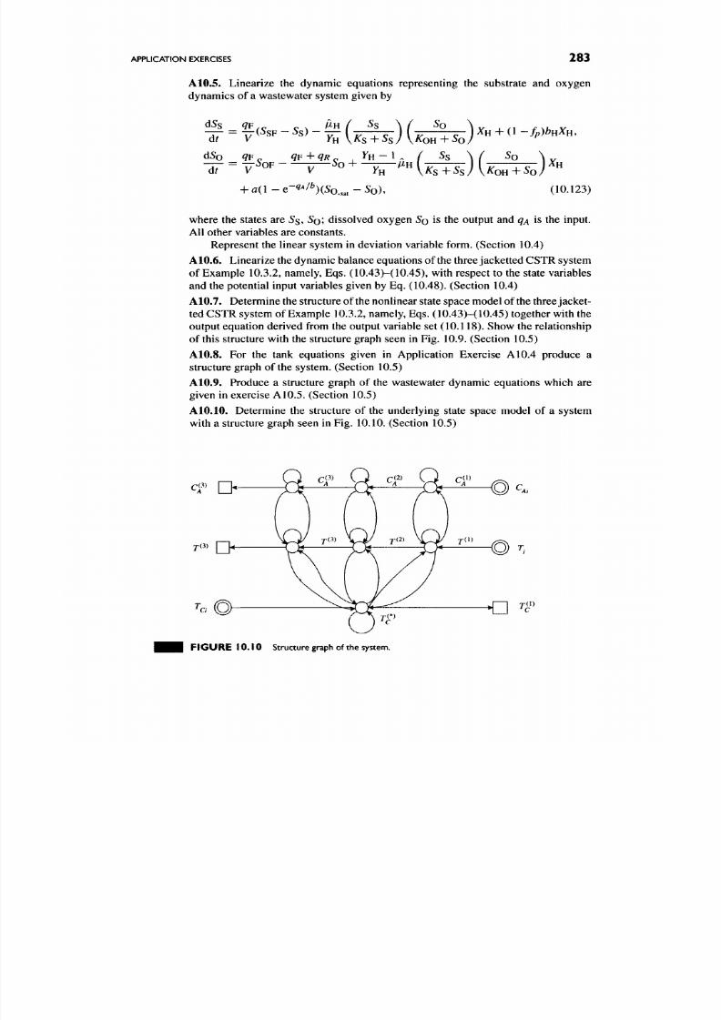
8/17/2019 Process Modelling and Model Analysis-Hangos-Cameron
http://slidepdf.com/reader/full/process-modelling-and-model-analysis-hangos-cameron 300/560
APPLICATION EXERCISES
283
A10.5.
Linearize the dynamic equations representing the substrate and oxygen
dynamics of a wastewater system given by
d5s 9F „ „
^ = y(5s F-5 s)
V/:s
+
5sJ v
d5o 9F „ ^F + 9/f „
YH-
+ a ( l - e - < ' ^ / ^ ) ( S o . 3 , - S o ) ,
l + SoJ
~^^ [KS+S S) [
XH
(10.123)
where the states are Ss, SQ; dissolved oxygen SQ is the output and ^^ is the input.
All other variables are constants.
Represent the linear system in deviation variable form. (Section 10.4)
A10.6. Linearize the dynam ic balance equations of the three jacketted C STR system
of Example 10.3.2, namely, Eqs. (10.43)-( 10.45), with respect to the state variables
and the potential input variables given by Eq. (10 .48). (Section 10.4)
A10.7. Determ ine the structure of the nonlinear state space model of
the
three jacket
ted CSTR system of Example 10.3.2, namely, Eqs. (10.43)-(10.45) together with the
output equation derived from the output variable set (10.118). Show the relationship
of this structure w ith the structure graph seen in Fig. 10.9. (Section 10.5)
A10.8. For the tank equations given in Application Exercise A10.4 produce a
structure graph of the system. (Section 10.5)
A10.9. Produc e a structure graph of the wastewater dynam ic equations which are
given in exercise A10.5. (Section 10.5)
AlO.lO. Determ ine the structure of the underlying state space model of a system
with a structure graph seen in Fig. 10.10. (Section 10.5)
c2' D
7(3) Q
T
7-(')
F I G U R E 1 0 . 1 0 Structure graph of the system.

8/17/2019 Process Modelling and Model Analysis-Hangos-Cameron
http://slidepdf.com/reader/full/process-modelling-and-model-analysis-hangos-cameron 301/560
284
CHAPTER
10
BASIC TOOLS FOR PROCESS MODEL ANALYSIS
A lO .l l. Produce the
LTI
state space model matrices
and
the input response function
of the following system model:
^ = 7 M I , (10.124)
at
- -± =
5JCI
+
-6JC2
+
8M3,
(10.125)
at
y\=xu
(10.126)
y2=X2.
(10.127)
Produce the structure graph of the system. (Sections 10.2 and 10.5)
8/17/2019 Process Modelling and Model Analysis-Hangos-Cameron
http://slidepdf.com/reader/full/process-modelling-and-model-analysis-hangos-cameron 302/560
DATA ACQUISITION
AND
ANALYSIS
There are a number of key steps in model building, namely model calibration and
validation and a number of key application areas, like process control and diagnosis
which depend critically on the quality of the available measured data. This chapter
gives a brief process oriented introduction to data acquisition and data analysis for
modelling, control and diagnosis purposes.
The outline of the chapter is as follows:
• Often we develop a continuo us time process model to be used for model cal
ibration and validation or control. The majority of estimation and/or control
methods require discrete time models. The sampling or discretization of usu
ally continuous time process models as an important model transformation
step for process param eter and structure estimation is outlined in Section 11.1.
• The quality of the estimates using model parameter and structure estimation
and sometimes even the success of these procedures depends critically on the
quality of the measurement data. Therefore, methods for assessing the quality
of collected data, i.e.
data screening
is briefly discussed in Section 11.2.
• M ost often we do not use measured data as collected, i.e.
passive data
from
the process system. W e usually artificially create data records sp ecially for the
estimation p urposes. The procedures w e use to design which experiments to be
carried out and how to get proper data for the estimation are called experimental
design procedures.
We shall review exp erimental design for static m odels, i.e.
design of steady-state data and experiment design for dynamic purposes in the
two subsequent Sections 11.3 and 11.4.
285
8/17/2019 Process Modelling and Model Analysis-Hangos-Cameron
http://slidepdf.com/reader/full/process-modelling-and-model-analysis-hangos-cameron 303/560
286 CHAPTER 11 DATA ACQ UIS ITION AND ANALYSIS
Although it is important to review the most commonly used experiment design
and data screening methods, no attempt is made in this section to give a detailed and
comprehensive description of them. The most important steps and procedures are
discussed from the viewpoint of process model calibration and validation. There are
a number of good books that interested readers may consult [72,73].
I . I . SAMPLING OF CONTINUOUS TIME DYNAMIC MODELS
Process models are usually constructed from balance equations with suitable consti
tutive equations . The balance equations can be either ordinary or partial differential
equations depending on the assumptions on the spatial distribution of process vari
ables. In order to solve balance eq uations, we need to discretize them som ehow both
in space (if needed) and in time. Spatial discretization methods have been discussed
in Chapter
8
on the solution of PDE models. This section discusses only discretization
in time assuming that we have already lumped our PDE model as needed. In other
words, only lumped process models are considered here.
The lumped balance equations are naturally continuous time differential equa
tions whereas almost any known method in m athematical statistics works with discrete
sets of data and uses underlying discrete time models. Therefore, the need to trans
form continuous time process models into their discrete time counterparts naturally
arises.
This type of time discretization is called sampling.
Almost any kind of data acquisition, data logging or control system is imple
mented on comp uters where continuous time signals are sampled by the measurement
devices. Control signals, generated by the com puter system in discrete time instances
are fed back to the process system to control it. Therefore, it is convenient to generate
the discrete counterpart of a process model by simply forming a composite system
from the original continuous time process system, the measurement devices taking the
sampled output signals and from the actuators generating the continuou s time manip
ulated input signals to the system as shown in Fig. 11.1. The box labelled S is the
original continuous time process system, the box
D/A converter
converts continuous
time signals to discrete time ones and the box A/D converter converts discrete time
signals to continuous time ones. The sampled data discrete time composite system
is in the dashed line box. The discrete time input and output variables (or signals)
to the discrete time system S^^^ are
u
:
[u{k)
=
u{tk)
I ^ = 0, 1,
2 , . . . } ,
(11.1)
j : M * ) = j a i t ) l ^
=
0 , l , 2 , . . . } ,
(11.2)
where
T
= {fo, ^i,
tj ,
...} is the discrete time sequenc e.
Most often equidistant zero-order hold sampling is applied to the system, w hich
means that we sample (measure) the continuous time signals and generate the
manipulated discrete time signals in regular equidistant time instances, i.e.
tk-^l-tk = h,
A: = 0 , 1 , . . . , (11.3)
where the constant h is the sampling interval. Moreover, a zero-order hold occurs in
the D/A converter to generate a continuous time manipulated input signal u{t) from
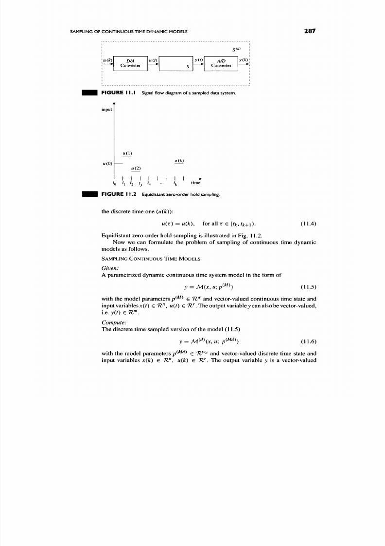
8/17/2019 Process Modelling and Model Analysis-Hangos-Cameron
http://slidepdf.com/reader/full/process-modelling-and-model-analysis-hangos-cameron 304/560
SAMPLING OF CONTINUOUS TIME DYNAMIC MODELS
287
: M ( / : )
D/A
Converter
t<(0
S
y(t)
— •
S(d)
:
A/D
Converter
y(k)l
F I G U R E 11.1 Signal flow diagram of a sampled data system.
input
M(0)
u(l)
w(k)
11(2)
0 h h h 4
I I I I I I
time
F I G U R E
11.2
Equidistant zero -ord er hold sampling.
the discrete time one
(u(k)):
U(T) = u(k), for all T e [tj,, tk^\).
(11.4)
Equidistant zero-order hold sampling is illustrated in Fig. 11.2.
Now we can formulate the problem of sampling of continuous time dynamic
models as follows.
SAMPLING CONTINUOUS TIME MODELS
Given:
A
parametrized dynamic c ontinuous time system m odel in the form of
y
=
M(x,u;p^^^)
(11.5)
with the model parameters p^^^
e
TZ^ and vector-valued continuous time state and
input variables x( 0 € TZ , u(t) e 7?.'\ The output variable j can also be vector-valued,
i.e.>'(0 eTV^.
Compute:
The discrete time sampled version of the model (11.5)
(11.6)
with the model parameters
p^^^^
e
IZ^"^
and vector-valued discrete time state and
input variables x(k) e TZ^, u(k) e W. The output variable j is a vector-valued
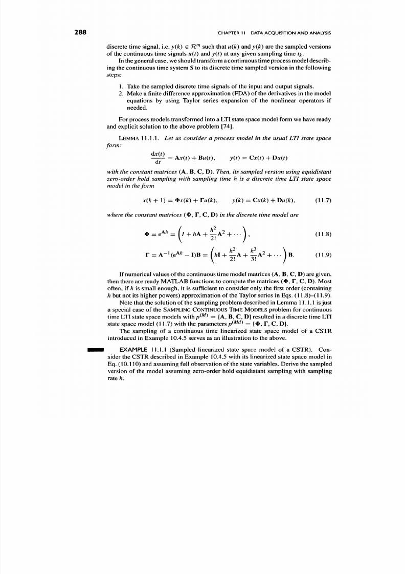
8/17/2019 Process Modelling and Model Analysis-Hangos-Cameron
http://slidepdf.com/reader/full/process-modelling-and-model-analysis-hangos-cameron 305/560
288 CHAPTER 11 DATA ACQ UIS ITION AND ANALYSIS
discrete time signal, i.e. y(k) e W ^ such that u{k) and y(k) are the sampled versions
of the continuous time signals
u{t)
and
y{t)
at any given sampling time
t^.
In the general case, we should transform a continuous time process m odel describ
ing the continuous time system S to its discrete time sampled version in the following
steps:
1. Take the sampled discrete time signals of the input and output signals.
2. Mak e a finite difference approximation (FDA) of the derivatives in the model
equations by using Taylor series expansion of the nonlinear operators if
needed.
For process m odels transformed into a LTI state space model form we have ready
and explicit solution to the above problem [74].
LEMMA 11.1.1. Let us consider a process model in the usual LTI state space
form:
Ax{t)
dr
=
AJC(0
+ BM(r), y{t) = Cx{t) + DM(r)
with the constant matrices
(A, B, C, D).
Then, its sampled version using equidistant
zero-order hold sampling with sampling time h is a discrete time LTI state space
model in the form
jc(jt + 1) =
^x{k)
+
Tu{k), y(k) = Cx{k)
+
Du{k),
(11.7)
where the constant matrices (^ , F, C, D) m the discrete time model are
4> = e^^ = f/ + /?A + ^ A 2 + . . . ] , (11.8)
u2 i3 \
/ i l - f — A + — A 2
+ . . . JB.
(11.9)
If numerical values of the continuou s time model matrices (A, B, C, D) are given,
then there are ready MA TLAB functions to compute the matrices (^ , T, C, D ). Most
often, if h is small enou gh, it is sufficient to consider only the first order (containing
h
but not its higher powers) approximation of the Taylor series in Eqs. (11.8 )-(11 .9).
Note that the solution of the sampling problem d escribed in Lemm a 11.1.1 is just
a special case of the SAMPLING CONTINUOUS TIME MODELS problem for continuous
time LTI state space models with/?^^^ = {A, B, C, D} resulted in a discrete time LTI
state space model (11.7) with the parameters p ^ ^ ^ ^ = {^, T, C, D}.
The sampling of a continuous time linearized state space model of a CSTR
introduced in Exam ple 10.4.5 serves as an illustration to the above.
EXAMPLE M .LI (Sampled linearized state space model of a CS TR ). Con
sider the CSTR described in Example 10.4.5 with its linearized state space model in
Eq. (10.110) and assuming full observation of the state variables. Derive the sampled
version of the model assuming zero-order hold equidistant sampling with sampling
rate h.
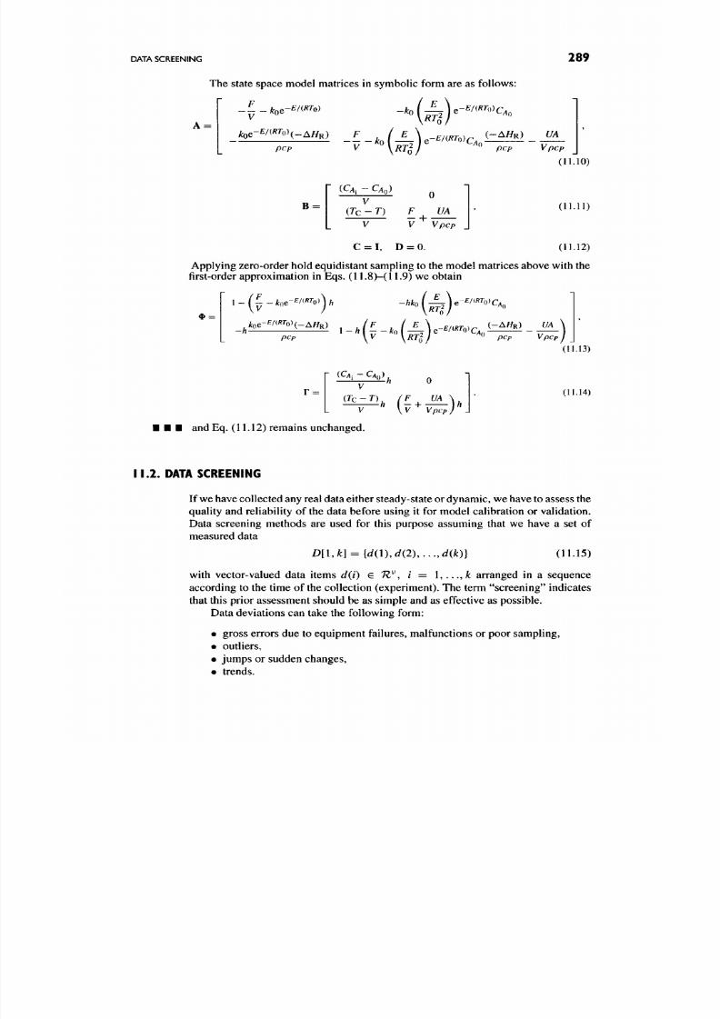
8/17/2019 Process Modelling and Model Analysis-Hangos-Cameron
http://slidepdf.com/reader/full/process-modelling-and-model-analysis-hangos-cameron 306/560
DATA SCREENING
289
The state space model matrices in symbolic form are as follows:
F
A =
V
kot-^n^^o)
-(4)
^-E/(RT,)c^^
i ^ e - ^ / ( ^ ^ o ) ( _ A ^ R )
pep
''y-'i-k}
mRT,)cj,^
{-AHR) UA
pep
Vpcp
(11.10)
B =
V
(Tc - T)
0
F UA
V " Vpcp
C = I, D = 0.
(11.11)
(11.12)
Applying zero-order hold equidistant sampling to the model matrices above w ith the
first-order approximation in Eqs. (11.8 )-(11 .9) we obtain
^>oe-^/<^^ o>(-Af/R) ^ ^
-h \-h
(-AHR) UA
pep
Vpcp
(11.13)
r
=
V
(7c - T),
/ F UA \^
[v^V^p)'
(11.14)
and Eq. (11.12) remains unchanged.
11.2 . DATA SCREENING
If
we
have collected any real
data
either steady-state
or
dynam ic, we have to assess the
quality and reliability of the data before using it for model calibration or validation.
Data screening methods are used for this purpose assuming that we have a set of
measured data
D[\,k] = {dil),d(2),...,d(k)} (11.15)
with vector-valued data items
d{i) e IZ ^, i =
1 , . . . , / : arranged in a sequence
according to the time o f the collection (experiment). The term "screening" indicates
that this prior assessment should be as simple and as effective as possible.
Data deviations can take the following form:
• gross errors due to equipment failures, malfunctions or poor sampling,
• outliers,
• jumps or sudden changes,
• trends.
8/17/2019 Process Modelling and Model Analysis-Hangos-Cameron
http://slidepdf.com/reader/full/process-modelling-and-model-analysis-hangos-cameron 307/560

8/17/2019 Process Modelling and Model Analysis-Hangos-Cameron
http://slidepdf.com/reader/full/process-modelling-and-model-analysis-hangos-cameron 308/560
DATA SCREENING
291
30 40 50 60
Time (minutes)
F I G U R E 11.3 Data visualization example No. I.
80 90
Instrument recalibration
40 60
Time (minutes)
F I G U R E 11.4 Data visualization example No. 2.
100
120
Two jumps forming a gross error are seen in Fig. 11.3. The reason for the gross
error was a measurement device failure: the corresponding automated sensor went
off-line when the first jump was observed and then went back online causing the
second jump.
The first part (in time) of the plot seen in Fig. 11.4 shows two big outliers and a
slow trend. These anomalies initiated a recalibration of the corresponding instrument
which is seen in the form of a positive jump on the plot.

8/17/2019 Process Modelling and Model Analysis-Hangos-Cameron
http://slidepdf.com/reader/full/process-modelling-and-model-analysis-hangos-cameron 309/560
292
CHAPTER 11 DATA ACQ UISITI ON AND ANALYSIS
11.2.2.
Outlier Tests
The notion of an outlier has no definite mathematical meaning in itself because
samples taken from a random variable with finite mean and variance, such as from
a Gaussian distribution may take very large value (theoretically of any magnitude)
with a very small probability. Therefore^we canjegard a measured data point as an
outlier if its relative m agnitude \\d(i)
—
d\\ with d as the sample mean and || • || as a
vector norm is much larger than the variance of the measurement errors
a^.
Apparent outliers are visible by data visualization but there are several outlier
tests we may apply (see [73]).
The outlier test methods are based on two different principles: either they are
looking for deviations from the "usual" distribution of the data
(statistical methods)
or they detect outlier data by limit checking. In both cases , we may apply the fixed or
the adaptive version of the methods depending on whether the normal (non-outlier)
data statistics are given
a priori
or they should be first estimated from test data.
1. Statistical methods
In this case, the outlier detection is based on probability distribution tests.
Assum e we know the probability density function pj(jc) of the data and have
a set of measured data D[l,k]Af the data items are independent of each other,
then we can regard the data set as a sample in a statistical sense and perform a
probability distribution test to check the hypothesis "Are these data from the
same und erlying distribution with probability density function/7^(jc)?".
In the case of
a
G aussian distribution the probability distribution test can
be performed using the well-known x^-test.
2. Limit checking
With these methods the signal sample mean d and the threshold for outlier
detection A^ =
CACTE
is either given
a priori
or it is estimated from time to
time over a sliding data w indow, given a fixed large constant C A > 3.
11.2.3. Trends, Steady-State Tests
If we want to perform a parameter and/or structure estimation of static models, then
we need to have steady-state data. Th is means no long or short term time v ariation in
the data sequence.
Steady state or stationarity includes the absence of trends.
There can be other circumstances when we want to have data with no trends.
This can be when trends are due to slow disturban ces. An examp le would be seasonal
changes which we do not want to model.
Trend detection and removal is therefore an important data screening procedure
and can be an efficient and simple process system diagnosis tool.
The trend detection or steady-state test methods can be divided into two grou ps:
methods based on parameter estimation and methods based on other statistics.
1. Methods based on parameter estimation
The simplest way to detect trends is to fit a straight line through the measured
data and check whether its slope is zero. If the measurement errors are inde
pendent of each other and are normally distributed, then standard statistical
hypothesis tests (see Section A.2 in the appendix) can be applied to check
their constant mean.
8/17/2019 Process Modelling and Model Analysis-Hangos-Cameron
http://slidepdf.com/reader/full/process-modelling-and-model-analysis-hangos-cameron 310/560
DATA SCREENING 293
2.
Me thods based on other statistics
The most well known and commonly used method is the so-called Cum ulative
SUMm ation (CUSU M) method. CUSUM is a recursive method which is based
on a recursive computation of the sample mean with growing sample size:
1 ^ 1
s[k] = ^Yld(i) = -i(k-l)s[k- U^dik)).
/=1
This cumulative sum based mean is then plotted against time and inspected
either by limit checking or by parameter estimation whether it has any slope
different from zero. It is important to n ote that the statistics s[k] of the CUSUM
method will have decreasing variance in time assuming data with the same
and constant distribution. Therefore, it becomes increasingly sensitive for
even small trends as time grows. Slow periodic changes, however, are simply
filtered out together with random measurement errors using these statistics.
Therefore, CUSUM is applicable only if a trend of constant slope sign is
expected.
More advanced methods on trend detection or testing the steady state can be
found in [73].
11.2.4. Gross Error Detection
Gross errors are caused by equipment failures or malfunctions. They can be detected
by different metho ds depen ding on the nature of the malfunctioning and on the pres
ence of other "health y" nearby sign als. The available methods for gross error detection
can be grouped as follows:
1.
Bias or slow trend detection
Gross errors can be visible bias or slow trend in the recorded signal of the sen
sor or sensors related to the equipment in question. Trend detection methods
(see above) can then be applied to detect them.
2. Jump detection
In case of sudden failure,
a
jump arises in the corresponding signal(s) which
can be detected via bias or jum p detection in time series by standard method s
[75].
The simplest methods are similar to those described in Section 11.2.2
for detecting outliers. For jump detection, however, only the fixed
a priori
configured version of the methods is applicable.
3.
Balance violation detection
The group of related signals of the equipment subject to failure or malfunc
tion can also be used for detecting gross error causing the violation of the
causal deterministic relationship between them. Static mass and energy bal
ances may serve for this purpose. These balances impose simple partial linear
relationships between the related signals of the equipment which can be used
for gross error detection [76].

8/17/2019 Process Modelling and Model Analysis-Hangos-Cameron
http://slidepdf.com/reader/full/process-modelling-and-model-analysis-hangos-cameron 311/560
294
CHAPTER 11 DATA ACQUISIT ION AN D ANALYSIS
11.3.
EXPERIMENT DESIGN FOR PARAMETER ESTIMATION OF STATIC MODELS
The parameter estimation for static models requires steady-state (or stationary) data
because of the model. Therefore, the first step in designing experiments is to ensure
and test that the system is in steady state. This
is
done by
steady-state tests as
described
in Section 11.2.3.
Thereafter, we decide the num ber of measurem ents, the spacing of the test points
and the sequencing of the test points.
11.3.1.
Number of Measurements
The number of measurements depends on the number of test points kp and on the
number of repeated measurements in the test points kR. One set of repeated m easure
ments at a particular test point is called an experimen t. If we repeat measu rements at
the test points, then we may have
a
good estimate on the variances of the measurem ent
errors w hich is very useful to assess the fit of the estimate (see in Section 12.2).
The number of test points depends critically on the number of state variables
of the process system and on the number of estimated parameters. In general, we
need to make sufficient measu rements to estimate unknown parameters and possibly
unknown states, i.e. the number of measurem ents shou ld be significantly greater than
the number of unknown parameters and states.
11.3.2. Test Point Spacing
It is important that we have a set of measu rements which "span" the state space of the
process system the model is valid for. This means that w e have to space ex perimental
measurem ent points roughly uniformly over the validity region of the process model
we are going to calibrate or validate.
It
is
equally important that
we
stay
within
the validity
region
of our process model.
For linear or linearized models, this validity region can be quite narrow around the
nominal operating point of the model. We may wish to perform linearity tests to find
out this validity region before we collect data for mo del calibration and v alidation.
11.3.3.
Test Point Sequencing
For static models and process systems in steady-state, the sequence of measurements
should not affect the result of parameter estimation. That is, because measurement
errors of the individual measurem ents are usually independent and equally distributed
with zero mean.
For some kinds of process systems, however, we can achieve the above nice
properties of independence and zero mean only by
randomization of the measure
ments. This artificially transforms systematic errors (biases, trends, etc.) into random
measurement errors. These kinds of process systems include
• systems with "bio" processes which may have a "memory-effect",
• systems which are affected by drifts or slow changes du e to unremovable
disturbances such as daily or seasonal changes.

8/17/2019 Process Modelling and Model Analysis-Hangos-Cameron
http://slidepdf.com/reader/full/process-modelling-and-model-analysis-hangos-cameron 312/560
EXPERIMENT DESIGN FOR DYNAMIC MODELS 295
11.4. EXPERIMENT DESIGN FOR PARAMETER ESTIMATION OF DYNAMIC MODELS
The experimental design for parameter and structure estimation of dynamic models
involves a number of additional issues compared with static models. The reason for
this is that we can only design the input variable part of the independent variables in
the model and then the output variables are determined by the dynamic resp onse of the
process system itself. In other words, the items in the measurem entsd(i), i = \,.. .,k
are
p artitioned into items belonging to input variables and output variables, i.e.
D[Uk] = {dd) I d(i) =
[y(i),
u(i)f, / = , . . . , k]
(11.16)
with vector-valued data items d(i) e 1Z^, y{i) e 7^'", u{i) e IV and v = m-\- r.
Moreover,
the sequence number of the particular m easured data should be interpreted
as discrete time. Therefore we cannot apply
Test
point sequencing. Moreover, Test
point spacing
can only be done in a constrained w ay taking into account the dynam ics
of the system.
The additional important issues in experiment design for parameter and/or
structure estimation of dynamic models include
• sampling time selection,
• excitation.
These are now discussed.
11.4.1. Sampling Time Selection
Proper sam pling of continuous tim e signals and process mod els is essential in the case
of parame ter and/or structure estimation of dynam ic mode ls. A detailed discussion on
sampling is given in Section 11.1 where we only deal with sampling time selection.
The selection of the sampling time is closely connected with the selection of the
number of measurem ents. We w ant to have sufficiently rapid sampling for a sufficient
length of time.
Mo reover, we wan t to have information ab out all time response characteristics of
our dynamic p rocess m odel, even about the fastest one w hich is usually the h ydraulic
effects or the component mass variations. For this reason
we have to select the sam
pling time to be roughly one third or one quarter of the fastest time response of the
process system,
which is usually in the order of seconds for process systems.
11.4.2.
Excitation
The dynamics of the process system should be sufficiently excited if we want to
estimate the parameters in a dynamic m odel. Although disturbances and other noise
sources are often p resent, the mag nitude and frequency of their variation is usually not
enough to give a good sign al-to-noise ratio for real plant measu reme nts. Therefore, w e
should apply som e kind of test signal on the inputs of the process system to generate
sufficient excitation. The lack of sufficient excitation may resu lt in a highly correlated
set of estimated parameters.
The most frequently applied signal is the so-called
pseudo-random binary
sequence (PRBS)
which gives reasonable excitation at very modest amplitudes but
requires a relatively long time period and does not disturb the normal operation of
the process system too m uch.
8/17/2019 Process Modelling and Model Analysis-Hangos-Cameron
http://slidepdf.com/reader/full/process-modelling-and-model-analysis-hangos-cameron 313/560
296
CHAPTER 11 DATA ACQUISIT ION AND ANALYSIS
The PRBS has only two signal magnitudes and jumps at randomly selected time
intervals from one to the other.
In designing the PRBS test signal [77],
• the base time interval and sampling time should be about one-fifth of the
smallest time con stant you w ish to identify;
• the sequence size should be chosen such that the sequence length is about five
times larger than the major time co nstant of the process system .
More about sufficient excitation, parameter estimation, identifiability and test
signal design can be found in [77].
11.5.
SUMMARY
The chapter gives a brief introduction to the preparatory steps of statistical model
calibration and validation.
The sampling of continuous time models prepares discrete time equivalents of
the developed process model needed for the model calibration and validation.
The basic methods and procedures for data analysis and preprocessing such
as data screening by visualization, steady-state detection, gross error and outlier
detection as well as experiment design for both static and dynamic process models
are outlined.
11.6.
FURTHER READING
Data acquisition and analysis is an important preliminary step in model calibration
and validation, and it is an important area with its own literature. Further reading in
this area is therefore only directed towards the aspects imp ortant from the viewpoint
of process modelling.
An interesting sub-field of data acquisition is the active learning from process
data in a process modelling context which has been reported in a recent paper [78].
The calibration and re-calibration of chemical sen sors is a vitally important issue
in obtaining good quality and reliable process data. This sub-field of data acquisi
tion and analysis mainly belongs to the field of analytical chemistry. An advanced
calibration method based on signal processing and curve fitting is reported in [79].
Data analysis is especially important when the standard Gaussian distribution
assumption of the measurement and other errors is known to be invalid. This is
usually the case for various faults and failures and has a special importance for risk
analysis. Sp ecial data analysis techniques are used to retrieve univariate distributions
from data for risk analysis [80].
11.7.
REVIEW QUESTIONS
Q l l . l . Describe briefly the available data screening procedures. Which ones are
applicable for a single signal and which on es for groups of signals? (Section 11.2)
8/17/2019 Process Modelling and Model Analysis-Hangos-Cameron
http://slidepdf.com/reader/full/process-modelling-and-model-analysis-hangos-cameron 314/560
APPLICATION EXERCISES
297
Q11.2.
Chara cterize briefly the outlier test metho ds. Which ones are applicable for
steady-state signals and which ones for slowly changing signals? (Section 11.2)
Q11.3. Describe briefly the principles behind the available gross error detection
methods. Describe the relation between them and the trend detection and outlier
detection methods. (Section 11.2)
Q11.4. What are the main points or questions to be considered when designing
experiments for parameter estimation for static models? (Section 11.3)
Q11.5.
W hat are the additional main points or questions to be considered comp ared
with the static case when designing exp eriments for parameter estimation for dynam ic
models? (Section 11.3)
11.8.
APPLICATION EXERCISES
A l l . l . Given a continuo us time LTI system model in the form of
dx
-— = AA: -f BM ,
y = CX
dr
with the matrices
- [ ^ :]• -
, C = [l 0] . (11.17)
Compute the sampled version of the above model. (Section 11.1)
A11.2. Investigate the plots in Figs. 11.3 and 11.4 by visual inspection and applica
tion of data screening methods. Mark clearly on the figure the time instance(s) and
signals(s) where you detect:
1. drift (slow change),
2.
oudiers,
3.
gross errors.
(Section 11.2.)
A11.3. Imagine the branching of a pipe in a piping system. Assum e that an incom
pressible fluid flows in the pipe in the direction of the branch where it divides into
two streams. The ratio between the cross sections in the pipes is 0.3:0.7 with the
cross section of the main pipe being 1. Give the static balances you can use for
gross error detection. Which sensors do you need to apply the method? What kind of
malfunctioning can you detect, if
1.
you know precisely the ratio between the cross section of the branched p ipes
as above,
2.
you do not know the exact ratio between them .
(Section 11.2.4.)

8/17/2019 Process Modelling and Model Analysis-Hangos-Cameron
http://slidepdf.com/reader/full/process-modelling-and-model-analysis-hangos-cameron 315/560
This Page Intentionally Left Blank
8/17/2019 Process Modelling and Model Analysis-Hangos-Cameron
http://slidepdf.com/reader/full/process-modelling-and-model-analysis-hangos-cameron 316/560
STATISTICAL MODEL
CALIBRATION AND VALIDATION
Model validation is one of the most difficult steps in the modelling process. It
needs a deep understanding of modelling, data acquisition as well as basic notions
and procedures of mathematical statistics. The aim of the chapter is to provide
the modeller with a user-oriented and hopefully also user-friendly basic under
standing of the most commonly used methods in statistical model calibration and
validation.
The outline of the chapter is as follows:
• The chapter starts with a revised and extended view of grey-box mod elling
in section 12.1 as a motivation for paying greater attention to parameter and
structure estimation in process modelling. The concept of model calibration
is introduced.
• Statistical model calibration is usually done through m odel parameter and/or
structure estimation. The basic notions about model parameter and struc
ture estimation are described in Section 12.2. The underlaying notions
and methods from mathematical statistics are given in Section A.l in the
appendix.
• Thereafter, the model param eter and structure estimation is discussed sep
arately for static and dynamic process models in Sections 12.3 and 12.4.
• Finally, mo del validation methods based on either mo del prediction or mo del
parameter estimation are discussed in Section 12.6.
299
8/17/2019 Process Modelling and Model Analysis-Hangos-Cameron
http://slidepdf.com/reader/full/process-modelling-and-model-analysis-hangos-cameron 317/560
300 CHAPTER 12 STATISTICAL MODEL CALIBRATION AN D VALIDATION
12.1.
GREY-BOX MODELS AND MODEL CALIBRATION
In practical cases, we most often have an incomplete model if we build a model from
first principles according to Steps 1 ^ of the
SEVEN STEP MODELLING PROCEDURE
described in Section 2.3. The reason for this is that we rarely have a complete model
together with all the parameter values for all of the controlling mechanisms involved.
An example of this is a case when we have complicated reaction kinetics, where
we rarely have all the reaction kinetic parameters given in the literature or measured
independently and often the form of the reaction kinetic expression is only partially
known.
This section deals with incomplete or grey-box models and with the procedure
called model calibration to make them solvable for dynamic simulation purposes.
12.1.1. Grey-box Models
The notion of grey-box modelling has been understood somewhat differently by vari
ous authors in the literature since the first book of Bohlin [81] appeared with this title.
It is used in contrast to the so-called empirical or black-box models when the model
is built largely from measured data using model parameter and/or structure estima
tion techniques (see for example [14,82]). The opposite case is the case of white-box
models when the model is constructed only from first engineering principles with
all its ingredients known as a well-defined set of equations which is mathematically
solvable. In practice, of course, no model is completely "white" or "black" but all of
them are "grey", since practical models are somewhere in between.
Process models developed using first engineering principles but with part of their
model parameters and/or structure unknown will be termed grey-box models in the
context of this book.
In order to illustrate how a grey-box model may arise consider a case of a
simple CSTR.
• • •
EXAMPLE 12.1.1 (A grey-box model of a CSTR). Consider a CSTR similar
to that of Example 10.3.1 with an exothermic reaction A —> B. The reaction rate
constant k is given by koc~^^^^ \ The reactor is cooled by coolant at temperature
7c.
It is assumed that inlet and outlet flows are equal, but we do not exactly know the
form of the reaction kinetic expression
rA=kc{CA). (12.1)
The functional form of c is unknown and we assume that the physico-chemical
properties depend on the temperature T but in an unspecified way, i.e.
cp = cp(T), p = p(T), A//R = A//R(r). (12.2)
Describe the grey-box model of the reactor.
The rearranged mass and energy balances lead to the following model equations:
(T - Tc). (12.4)
= ^(70) -
-CA)-rA,
- T) - I^(-AHK) -
pep
UA
V pep

8/17/2019 Process Modelling and Model Analysis-Hangos-Cameron
http://slidepdf.com/reader/full/process-modelling-and-model-analysis-hangos-cameron 318/560
GREY-BOX MODELS
AN D MODEL
CALIBRATION
301
Now the grey-box model of the CSTR consists of the two balanc es above (1 2.3 )-( 12.4)
with the following unknown structural elements:
1.
reaction kinetic expression as in Eq. (12.1),
2.
property relations as in Eqs . (12.2).
12.1.2. Model Calibration
It follows from the above that we often do not have available values of the model
parameters and/or part of the model structure. Therefore, we want to obtain these
model parameters and/or structural elements using experimental data from the real
process. Because m easured data contain measurement errors,
we
can only estimate the
missing model parameters and/or structural elements. This estimation step is called
statistical model calibration.
From the above description, we can conclude that the model calibration is
performed via a model parameter and/or structure estimation using
• the developed grey-bo x model by the steps 1-4 of the SEVEN STEP MODELLING
PROCEDURE,
• measured data from the real process system which we call
calibration data,
• a predefined m easure of fit, or
loss function
which measures the quality of
the process model with its missing parameters and/or estimated structural
elements.
A m ore precise list of the ingredients above will be given in the problem statement
of model parameter and structure estimation in the next section.
Conceptual Steps of Model Calibration
In realistic model calibration there are other important steps which one should carry
out besides just a simple model parameter and/or structure estimation. These steps
are needed to check and to transform the grey-box model and the measured data to a
form suitable for the statistical estimation and then to check the quality of the obtained
model. These conceptual steps to be carried out when doing model calibration are as
follows:
1.
Analysis of model specification
Here, we have to consider all of the ingredients of our grey-box process
model to determine which parameters and/or structural elements need to be
estimated to make the process model equations solvable for generating their
solution as a vector for static models or as a vector-valued function of time
for dynamic models. This step may involve a DOF analysis and the analysis
of the non-measurement data available for the model building.
2.
Sampling of continuous time dynamic mod els
Statistical procedures use a
discrete set of measured da ta
and a mo del. To get
an estimate therefore we need to discretize our grey-box process models to
be able to estimate its parameters and /or structural elements (see Section 11.1
for details).

8/17/2019 Process Modelling and Model Analysis-Hangos-Cameron
http://slidepdf.com/reader/full/process-modelling-and-model-analysis-hangos-cameron 319/560
302 CHAPTER 12 STATISTICAL MODEL CALIBRATION AN D VALIDATION
3. Data analysis and preprocessing
Measurement data from a real process system are usually of varying qual
ity. We may have data with bias, outliers or large measurement errors due to
some malfunctions in the measurem ent devices or unexpectedly large distur
bances. From the viewpoint of good quality estimates it is vital to detect and
remove data of unacceptable quality. (The methods for this are described in
Section 11.2).
4.
Mode l parameter and structure estimation
5. Evaluation of the quality of the estimate
The evaluation is done by using either empirical, usually graphical methods
or by exact hypothesis testing if the mathematical statistical properties of the
estimates are av ailable. M ore details w ill be given about the measure of fit in
Section 12.3.
Mod el calibration is usually followed by model validation when w e decide on the
quality of the model obtained by modelling and model calibration. Model validation
is in some sense similar to model calibration becau se here we also use measured data,
but another, independently measured data set
{validation data)
and also statistical
method s. Model validation is the subject of the last Section 12.6.
12.2.
MODEL PARAMETER AND STRUCTURE ESTIMATION
The estimation of some or all of the model parameters and/or parts of the model
structure is the technique we use in the mod el calibration and in the model validation
steps of
the
SEVEN STEP MODELLING PROCEDURE.
During
model
calibration
we use the
developed grey-box model and measured experimental data to obtain a well-defined
or solvable process model. In the
model validation
step, we again use measured
experimental data (the validation data) distinct from what has been applied for mod el
calibration. We do this in two different ways :
• to com pare the predicted outputs of the model to the measured data, or
• to comp are the estimated parameters of the model based on validation data to
the "true'' or previously estimated parameters.
12.2.1. The Model Parameter Estimation and the Model Structure
Estimation Problem
The conceptual problem statement of the model parameter estimation and model
structure estimation is given below :
MODEL PARAMETER ESTIMATION
Given:
• A parametrized explicit system model in the form of
j W =
M{x\ p^^^)
(12.5)
with the model parameters p^^ e
TV
being unkno wn, the vector-valued inde
pendent variable
x eTV^
and vector-valued dependent variable
y^^^ e IZ^.
8/17/2019 Process Modelling and Model Analysis-Hangos-Cameron
http://slidepdf.com/reader/full/process-modelling-and-model-analysis-hangos-cameron 320/560
MODEL PARAMETER AND STRUCTURE ESTIMATION
303
• A set of measu red data
D[0,
k] = {(jc(/), >^(/))
I
/ = 0 , . . . , / : } , (12.6)
where
y{i)
is assumed to contain measurement error while
x(i)
is set without
any error for static models and may contain ad ditional measurem ent errors for
dynamic models.
• A suitable signal norm
||
• || to measure the difference between the model output
y^^^ and the measured independen t variables
y
to obtain the loss function of
the estimation:
L(p)==\\y-y^^^\\.
(12.7)
Compute:
An estimate p^^^
ofp^^^
such that
L(p)
is a minimum:
| | ^ _ ^ W | | - ^ m i n .
Some of the items in the above problem statement need further discussion and
explanation as follows.
1. The measured values of the dependent variable {y(i),
i =
1,...,/:} are
assumed to have a zero mean measurem ent error. That
is
y(0 = y^^^
(i)
-\-s(i)
with
£
being the measurement error while the independent variables are
assumed to be set error-free for static models and may contain additional
measurement error for dynamic m odels. In other words,
{y(i),
i = 1 , . . . ,
A;}
is a sequence of random variables and the sequence {x(i),
i = I,.. .,k} is
either deterministic in case of static models or stochastic.
2.
No te that the estimate
p^^^
itself
is
also a random variable. The quality of the
estimate ^ ^ ^ \ or the properties of its mean value, variance and its distribution
depends on
(a) the parametrized m odel form, whether it is linear, nonlinear, etc.,
(b) the signal norm selected,
(c) the actual estimation procedure applied,
(d) selection of the independent variable values, as given by the selection of
the sequence {JC(0, / = 1 , . . . , k}.
The proper selection of the independent variable values is the subject of
experimental design.
3.
The general loss function defined in Eq. (12.7) has more meaningful forms.
For example, in practical cases it is the sum of the squares of the difference
between y and y^^\ The notion of vector and signal norm s is introduced in
Section A.3 in the appendix and some simple examples are also given there.
4. It is also im portant to note that the MO DEL PARAMETER ESTIMATION problem is
an optimization prob lem. We want to minimize the loss function in Eq. (12.7)
which depends on the model parameters
p^^^
in an implicit way through
Eq. (12.5).
MODEL STRUCTURE ESTIMATION
Given:
•
An explicit (but not param etrized) system model in the form
jW = M(x) (12.8)

8/17/2019 Process Modelling and Model Analysis-Hangos-Cameron
http://slidepdf.com/reader/full/process-modelling-and-model-analysis-hangos-cameron 321/560
3 0 4 CHAPTER 12 STATISTICAL MODEL CALIBRATION AN D VALIDATION
with the model M being an unknown form of the vector-valued independent
variable
x elZ^
and vector-valued dependent variable
y^^^ e 1Z^.
• A set of measured data
D[0,
k]
=
{(jc(0,
y(i))
\i =
0,..,,k}
(12.9)
where ^(0 is assumed to contain measurement error while JC(/) is set without
any error for static models and m ay contain additional m easurement errors for
dynamic models.
• A II • II a signal norm to measure the difference between the model ou tput y^^^
and the measured variables
y
to obtain the loss function
L(M)
in the form of
Eq.(12.7).
Compute: ^^
An estimate MofM such that L(M) is minimum
| | ^ _ v W | | - > m i n .
It can be seen from the above problem statement that the task of model structure
estimation is much more com plex than the task of model parameter estimation. M ore
over, the problem statement above is ill-defined in the mathem atical statistical sense
because even non -parametric statistical methods need to have a well-defined domain
of the non-parametric function in order to be estimated. This is usually a p robability
density function. Therefore, we usually constrain the domain, D o m ^ of the models
M
in the non-parametric explicit model equation (12.8) to have a finite set of explicit
parametric system models (12.5). In other words, we give the set of possible model
structures
when constructing the domain D o m ^ :
Dom^ = {Mi{x;pf^),.,.,MM{x;p^M^)}.
(12.10)
It follows from the above that if the model structure estimation problem is con
strained
by the set of
possible model structures, then
the
conceptual solution
of
the model parameter estimation problem breaks down to considering the number of
candidate model structures. Therefore, the conceptual solution of a model structure
estimation problem consists of the following steps,
1. Construction of the set of candidate model structures (12.10).
2. Model parameter estimation for every model
Mm^
m = 1,..., Af in the set
and the computation of the corresponding loss function Lmipin ) in the form
of Eq. (12.7).
3. Selection of the member M^ with the minimal loss L^ipi ). Note that
together with the "best-fit" model structure of A^*, we obtain an estimate
of its parameters
pi
as
a
side effect.
Finally, we illustrate the way the above problem specifications can b e constructed
by
a
simple exam ple.
EXAMPLE 12.2.1 (A model structure estimation problem of a CSTR). Consider
the CSTR described
in
Example
10.3.1,
i.e. consider
a
CSTR with
an
exothermic
8/17/2019 Process Modelling and Model Analysis-Hangos-Cameron
http://slidepdf.com/reader/full/process-modelling-and-model-analysis-hangos-cameron 322/560
MODEL PARAMETER AND STRUCTURE ESTIMATION
305
reaction
A
—
> B.
The reaction rate constant
k
is given by
koQ~^^^^.
The reactor is
cooled by coo lant at temperature 7 c . It is assumed that the physical properties remain
constant and that inlet and outlet flows are equal. Assume we have several candidate
reaction kinetic expressions:
1. rA =kCA,
2. rA = kCj(
,
3.
rA = kCAliCl -
Q ) .
Describe the set of candidate model structures, i.e. D o m ^ for model structure
estimation.
The rearranged m ass and energy balances lead to the following model equ ations:
At
T 7 (Q - Q ) - ^ A , (12.11)
d r
F
.:x
rA UA
=
-{T^'^
-T)-
- ^ ( - A / / R ) -
(T
-
Tc ). (12.12)
at V pep \ pep
Now the
set of candidate model structures
D o m ^ = { A l i, wM2» A^a) consist
of the two parametrized model equations with their parameters unknown:
1. Mi: Eqs. (12.11)-(12.12 ) with r^
=
kCA,
2. M 2 : Eqs. (12.11)-(12,12) with r^ =
kc\^^,
• • • 3 . A t a : E qs . (1 2.11 )-( 12 .1 2) w ith r ^ = i t Q / ( C ; - C A )
12.2.2.
The Least Squares (LS) Parameter Estimation for Models
Linear in Parameters
The least squares (LS) estimation methods receive their name from the square signal
norm || • II2 which is applied for com puting the loss function in Eq. (12.7):
L(p)=iij-jW |i2 ^ E E ( ^ i « - ^ r » ) '
\i=O j=\
As w e see later in this chapter, almost every parameter or structure estimation problem
for models linear in their parameters is somehow transformed to
a
standard least
squares parameter estimation problem. Therefore, this estimation procedure and its
properties are of primary importance and will be described and analysed.
Problem Statement
The LS parameter estimation problem statement for models linear in their parameters
and with a single dependent variable is as follows:
L E AS T
SQUARES ESTIMATION (LI fEAR IN PARAMETER SINGLE DEPENDENT VARIABLE
MO D E L S )
Given:
• A linear in param eter system model in the following form:
n
ym ^Tp^j XiPi (12.13)
1=1
8/17/2019 Process Modelling and Model Analysis-Hangos-Cameron
http://slidepdf.com/reader/full/process-modelling-and-model-analysis-hangos-cameron 323/560
306
CHAPTER 12 STATISTICAL MODEL CALIBRATION AN D VALIDATION
with the model parameters
p e
TV being unknown, the vector-valued inde
pendent v ariable x E 7^" and scalar-valued dependent variable y^^^ e 1Z.
A
set of measured data consisting of
m
measurements (m >
n)
arranged in a
vector-matrix form as
(12.14)
y\
yi
ym
, x =
^11
X2\
^m\
XX2 '
xn '
^ml '
• Hn
' X2n
^mn
where yi is assumed to contain measurement error.
A loss function L
m m
L(p) = rTW r = ^ ^ r / W ^ o ,
n=yi~ y-
(M)
(12.15)
(12.16)
where
r
is the
residual vector
and W is a suitable
positive definite symme tric
weighting matrix.
Compute:
An estimate
p ofp
such that the loss function
L(p)
is a minimum.
The LS Parameter Estimation Method
The LS parameter estimate for
p
is in the form of
(X'^WX)^ = X'^W j or p=:(X'^WX)-^X'^W >;.
(12.17)
Note that the two forms are mathematically equivalent but they are used for
different purposes:
1.
For parameter estimation, wh ere we com pute the estimate p, the implicit form
shown on the left-hand side is used. This allows us to use regularization and
decom position m ethods to solve the overdetermined linear equation resulting
in a much better and numerically stable procedure even for ill-conditioned
cases.
2.
The explicit form shown on the right-hand side is only for theoretical analysis
purposes. The statistical properties of the estimate
p
will be analysed using
this form.
Extension to the Vector-Valued Dependent Variable Case
A linear in parameter model in the form of (12.36) can be extended to the case of
vector-valued dependent variable y^^^ e Vy
.m
=
P J C ,
(12.18)
where the matrix of model parame ters P €
TV^^^^
contains the model para
meters of the subm odel belon ging to the 7th entry of the vector j ^ ^ ^ in its rows
8/17/2019 Process Modelling and Model Analysis-Hangos-Cameron
http://slidepdf.com/reader/full/process-modelling-and-model-analysis-hangos-cameron 324/560
MODEL PARAMETER AND STRUCTURE ESTIMATION
307
The above model can be transformed into the form required for the parameter
estimation of the single depen dent variable case in (12.14) if one forms the following
vectors and data matrices:
(12.19)
where j /y ) is the jth entry of the ii h measured dependen t data vector which is assumed
to contain measurement error.
Handling Measurement Errors
There are several important remarks and observations which sho uld be discussed co n
cerning the LEAST SQUARES ESTIMATION (LINEAR IN PARAMETER MODELS) problem
which are as follows.
1. Most often the measured dependent variable values are assumed to have an
additional measurem ent error with zero mean, i.e.
>'l(l)
yuv)
Jm(l)
ym(v)
. p =
Pn
P\n
Pv\
_ Pvn
, x* =
X
0
0
0 ••
X
0 ••
• 0
0
X
yt
E{8i}
y]
+^M
0.
/ = 1 , . . . ,m,
(12.20)
(12.21)
where E{.} is the mean value operator. If in addition the individual measurement
errors are statistically independent of e ach other and
are
normally distributed with a
diagonal covariance matrix Ag, then we can characterize the Gaussian distribution
of the measured values as
y-^Af(y^^\Ae), (12.22)
i.e. the measured value vector is also normally
distributed. Note that in the vector-
valued dependent variable case the above assumption means that the measurement
errors of the vector entries are independent in addition to the independence of the
measurement errors in the individual measurement points.
2. One of the most difficult problems in specifying a weighted least squares
parameter estimation prob lem is to choose the weights properly. The weigh ting matrix
W in the loss function L given by Eq. (12.15) is used to impose a different weight
on the residuals of the particular measurement points. If some of the measurement
points are regarded as relatively unreliable, such that their measurement error has a
larger variance, then it is assigned a lower weight com pared to the others. An obvious
choice for the weighting matrix is to select it to be the inverse of the covariance matrix
of the measurement errors if it is known or its estimate can be obtained:
W
. - 1
(12.23)
Note that the inverse matrix above always exists because covariance matrices are
positive definite.

8/17/2019 Process Modelling and Model Analysis-Hangos-Cameron
http://slidepdf.com/reader/full/process-modelling-and-model-analysis-hangos-cameron 325/560
3 0 8 CHAPTER 12 STATISTICAL MODEL CALIBRATION AN D VALIDATION
12.2.3.
Properties of
LS
Parameter Estimation
We can look at the explicit form of the estimation equation (12.17 ) as being a linear
transformation of the random variable y by a constant, non-random matrix
T=:(X'^WX)-^X'^ (12.24)
in order to get the random variable p. Th erefore, we can com pute the mean value and
the covariance matrix of the estimate
p
following the formulae (A. 13) described in
section A . 1.2 in the appendix as
CO\{p] = TCO V{ j}T^. (12.25)
If
the
measurement errors are normally distributed with zero mean and covariance
matrix
A^
and
the
weighting matrix in the loss function Eq. (12.15) h as been selected
accordingly as in Eq. (12.23) then the estimate p has the following properties:
•
It is normally
distributed.
• Its mean value is E[p] = p , hence it is
unbiased.
•
Its covariance matrix is computed as
CO\{p] = (X'^W X)-^A ^. (12.26)
• The estimate itself is a maximum -likelihood estimate, and thus an efficient
optimal estimate.
Confidence Intervals and Regions for the Estimated Parameters
The covariance matrix of the estimate COV{p} contains information not only on the
variances of the individual entries
pi
(being the diagonal elements of it) but also on
the correlation between the estimates. As has been said before, if the measurement
errors are statistically independent of each other and are normally distributed with
zero mean and covariance matrix A^, with the weight matrix W set accordingly then
the distribution of the estimate p is Gaussian w ith the covariance matrix in Eq. (12.26).
In order to understand what the covariance m atrix m eans about the quality of the
estimate in the case of two parameters, we can look at the shape of the 2D Gaussian
probability density function shown in Figure A.2 in Section A .l in the appendix. The
elements in the covariance matrix determine the shape of the ellipsoidal cuts of the
function and the direction of the main axis of the ellipses. In the case of more than
two parameters the confidence
region
is a m ulti-dimensional ellipsis with parameters
being the lengths of its axes and the direction of its main axis. Note that the lengths
of the axes have nothing to do w ith the variances of the param eter vector entries.
Unfortunately, we can not con struct confidence intervals separately in the strict
mathematical sense for the normally distributed parameters in this case and give an
estimate of the covariance or correlation between any pair using the off-diagonal
elements. This was only possible if the estimate p contained independent entries.
In order to overcome this difficulty we may apply two different approaches to
have information on the confidence region and confidence intervals for the estimated
parameters.
8/17/2019 Process Modelling and Model Analysis-Hangos-Cameron
http://slidepdf.com/reader/full/process-modelling-and-model-analysis-hangos-cameron 326/560
MODEL PARAMETER AN D STRUCTURE ESTIMATION
309
1.
Linear transformation of the estimated parameter vector
Similar to the standardization of vector-valued rando m variables described in section
A.
1.3 in the appendix the vector-valued transformed parameter vector
p*
= CO\{p}-^/^p-p
(12.27)
is approximately a standard Gaussian vector-valued random variable (see Sec
tion A. 1.1 in the append ix). This means that its entries are regarded as independ ent
random variables with standard Student r-distribution. This distribution can be used
to construct confidence intervals for the entries independently on the given signifi
cance level. The Student
t-test
can be used for testing hypotheses independently for
the mean value of the
transformed
parameter values.
Note that by this transformation we transform the multidimensional ellipse
as
confidence region in the space of the original param eters into a multivariable rectangle
which is parallel to the co-ordinate direction in the space of transformed variables.
Thereafter, the inverse of the standardization transformation (12.27) above can
be used
to
transform back the m ultivariate rectangle into the space
of
the original
param eters. With the vectors of lower and upper confidence limits of the transformed
parameters p ^ and ^ ^ , we get the following lower and upper parameter vectors for
the original parameters:
PL
= CO V{p}>/2p* +p,
py j
= COV{p}>/2p5 +p. (12.28)
2.
Individual confidence intervals
It is possible to construct
a
statistically
corvQci joint confidence region for all of the
parameters
on the (1 — a) significance level as follows:
(pirn
_pfx^WXip^^^ -p)<
vs^F{v, k-v,l-a), (12.29)
where
F(v, fc —
y, 1 — a ) is the (1 — a ) point
("upper
a point") of the F(v, k — v)
distribution value for DOF (v, k — v) and
s^
is the estimated (empirical) standard
deviation as an estimate for the variance of the measurement errors computed from
the data. The F( v,
A;
— v , 1 — a) value can be obtained from standard statistical tables,
where v is the numerator and ^ — v is the denominator.
The inequality above is the one which provides the equation of an "elliptically
shaped" contour in the space of all parameters.
In order to derive some kind of average individual confidence intervals for the
param eters we first observe that the worst-case confidence intervals for the individual
parameters would be the vertices of the multidimens ional re ctangle parallel to the
co-ordinate directions and containing the whole multidimensional ellipsis. For very
long and thin ellipses, however, this would be a very conservative estimate and the
majority of this multi dimensional cube would not represent a reasonable parameter
vector. This situation is seen on Fig. 12.1 in the case of two param eters w ith point E.
Note that if we construct more reasonable average confidence intervals then the
same situation will also arise with the presence of non-valid parame ter vectors w ithin
the volume permitted by the Descartes product of the individual confidence intervals
which is a smaller cube within the conservative one. Moreov er, we shall have left out
some of the valid parameter vector values. See point A in Fig. 12.1.
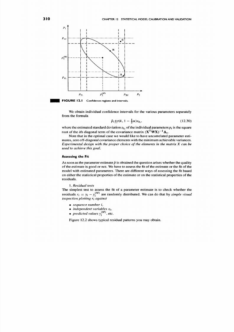
8/17/2019 Process Modelling and Model Analysis-Hangos-Cameron
http://slidepdf.com/reader/full/process-modelling-and-model-analysis-hangos-cameron 327/560
310
CHAPTER 12 STATISTICAL MODEL CALIBRATION AND VALIDATION
PlL Pi PlX}
FIGURE 12 .1 Confidence regions and intervals.
We obtain individual confidence intervals for the various parameters separately
from the formula
Pi±t{k, 1 - \ot)sb..
(12.30)
where the estimated standard d eviation
5^.
of the individual parameters
p/
is the square
root of the /th diagonal term of the covariance matrix (X^WX)~^ A^.
Note that in the optimal case w e would like to have uncorrelated param eter esti
mates, zero off-diagonal covariance elemen ts with the minimum achievable variances.
Experimental design with the proper choice of
the
elements in the matrix X can be
used to achieve this goal.
Assessing the Fit
As soon as the parameter estimate p is obtained the question arises w hether the quality
of the estimate is good or not. We have to assess the fit of the estimate or the fit of the
model w ith estimated param eters. There are different ways of assessing the fit based
on either the statistical prope rties of the estimate or on the statistical prop erties of the
residuals.
1.
Residual tests
The simplest test to assess the fit of a parameter estimate is to check whether the
residuals r/ = j / — y- are randomly distributed. We can do that by simple visual
inspection plotting r/ against
•
sequence number i,
• independent variables Xj,
. (^)
etc.
predicted values
yI
Figure 12.2 shows typical residual patterns you may obtain.

8/17/2019 Process Modelling and Model Analysis-Hangos-Cameron
http://slidepdf.com/reader/full/process-modelling-and-model-analysis-hangos-cameron 328/560
MODEL PARAMETER AND STRUCTURE ESTIMATION
311
+ + JC
random
+ + + + ^ ,
^ . ^
non-random
F IG U R E 12. 2 Residual patterns.
If we can assume that the measurement errors are statistically independent of
each other and are normally distributed with zero mean covariance matrix Ag then
the residuals can be regarded as a sam ple
to test the hypothesis
S{E) = { r i , r 2 , . . . , r ^ t )
Ho:m = 0
by standard hypothesis testing (see details in Section A.2 in the appendix).
In case of a single dependent variable with known variance A ^, we can compute
the test statistics
u
as in Eq. (A. 18) Section A.2 in the appendix. Otherwise, we
compute the empirical sample variance
A ,.s^ , SW ) = E - ' ' ^ ' - ' ^ l ^ « » '
m
—
I
with M{S(£)} being the sample mean as in Eq. (A. 17)
M{S(£)} =
^^if- -.
k
Thereafter, we can compute the test statistics
M{ S(£)} - mo
(12.31)
v^^lSCi)}
~ f . - l ( 0 ,
1).
(12.32)

8/17/2019 Process Modelling and Model Analysis-Hangos-Cameron
http://slidepdf.com/reader/full/process-modelling-and-model-analysis-hangos-cameron 329/560
3 1 2 CHAPTER 12 STATISTICAL MODEL CALIBRATION AN D VALIDATION
where the test statistics t has a standard Student r-distribution ^v_i (0, 1) and perform
a Student r-test.
The case of vector-valued dependent variable is much more complicated and
needs the full arsenal of multivariate statistics [83]. In the case of Gau ssian m easure
ment error distribution the so-called Wilks test [84] is used instead of the
u
test for
testing hypothesis on the mean value with known covariance matrix.
If the residuals are found to be non-randomly distributed and /or the residual tests
have failed then we have problems with either the model or the data or both.
2.
Correlation coefficient measures
In order to compute the correlation coefficient measures we have to decompose the
sum of squares (SOS) about the sample mean
ImSOS
into two parts
(IrSOS
+ Idsos)
as follows:
/SOS = E Cy/ - M{y})2 = ^ (y, -
yf^f +
J2(yf^
- M{y}9
(12.33)
i=\ i=\ i=\
with
M{y} = lJ2y- ' ^ S G S ^ E l ^ ' - ^ n ^ ldSOS = i:(yf'-M{y})^
^ i=\ i=\ i=\
and M{y} being the sample mean of the measured depen dent variables. In this decom
position, / so s is the total variation w hich is decom posed to the unexplained variation
^ SOS about regression and to the explained variation Idsos due to regression. The
coefficient of determination
and its square root
/0 =
L?=, ( r -M{y)f
NJ E?=iO'--M{3'})2
measures the variation in the data explained by the model.
12.2.4. The LS Parameter Estimation for Nonlinear Models
If we have a model nonlinear in its parameters then we can apply two different
techniques to estimate its parameters.
1.
Transform the nonlinear model into a form which is linear in its parameters
and apply LEAST SQUARES ESTIMATION (LINEAR IN PARAMETER MODELS).
2. Solve the general MODEL PARAMETER ESTIMATION problem.
If we cannot transform the model equations into a form linear in parameters
then we have to solve the general nonlinear model parameter estimation problem.
As it has been mentioned before the MODEL PARAMETER ESTIMATION problem is an

8/17/2019 Process Modelling and Model Analysis-Hangos-Cameron
http://slidepdf.com/reader/full/process-modelling-and-model-analysis-hangos-cameron 330/560
MODEL PARAMETER AND STRUCTURE ESTIMATION
3 I 3
optimization problem with the following ingredients:
• a process model nonlinear in parameters y^^^ = Mix; p),
• a set of measured data D[0 ,
k]
as in Eq. (12.6) and a set of predicted model
outputs
[y^^^{i),i = I,.. .,k]
com puted from the model equation above using
the measured values of the independent variables { x(0, / = , . . . ,
k],
• a loss function in the LS parameter estimation case in the form of SO S
k
Lsosip) = E Il3^« - / ^ ^ « l l 2 . (12 .35)
which is a special case of the general loss function in Eq. (12.7) depending on
the model parameters
p
in an implicit way through the model equation above.
The optimization problem above is usually solved by a suitable optimization
algorithm, most often by the Levenberg-Marquardt
method.
It is important to note that the
estimate p has lost its nice statistical properties
mentioned in Section 12.2.3. Therefore the lack of fit tests can only be applied with
caution and their results taken as approximate in the case of models nonlinear in
parameters.
Confidence Intervals and Regions for the Estimated Parameters
As has been m entioned, the LS estimate p do es not have the nice statistical p roperties
in the case of models nonlinear in their parameters as in the case of models linear in
parameters.
Therefore we can only apply an
approximate approach
if we want to estimate
the parameter confidence intervals for the estimated coefficients. T he theory given in
Section 12.2.3
is
not sufficient
to
cover this issue
as the
estimated parameter confidence
intervals are only applicable to linear models. The following explains a possible
approach for the single parameter case to get the nonlinear parameter confidence
interval.
This approach requires us to graph the sum of squares value (Lsos) as a function
of the parameter to be estimated
p
as seen in Figure 12.3.
Figure 12.3 shows the optimum value of popt and its LS value Lopt- A 95%
confidence level for the sum of squares can be established using:
where in the single-dependent variable case:
k
r ^r = J2^(i)-y(i)^)^=L opt
i=\
and k = number of data points, v = num ber of parame ters (now v = 1), and
F(y ,
k
—
v,
0.05) is the
F
distribution value for DOF (v,
k
— v). This can be obtained
from standard statistical tables, w here v is the num erator and k
—
vi s the denominator.
Once the SOS95 line has been drawn on the above figure, it is then possible to
estimate the parameter confidence interval by simply taking the intersection points
on the
S OS
line.

8/17/2019 Process Modelling and Model Analysis-Hangos-Cameron
http://slidepdf.com/reader/full/process-modelling-and-model-analysis-hangos-cameron 331/560
314
CHAPTER 12 STATISTICAL MODEL CALIBRATION AND VALIDATION
Parameter/?
F IGURE 12 .3 Nonlinear
SOS
variation.
Note that in the case of a nonlinear problem^ the SO S curve will not be symmetric
about
the
/7opt
value.
We may generalize the above method for constructing confidence intervals indi
vidually in case of more than one parameter to be estimated. We have to take these
confidence intervals with the same conc erns as described in Section 12.2.3 for linear
models. The
joint confidence
region
for the estimated parameters for models non
linear in parameters, however, will not be a multidimensional ellipses. It may be
non-convex of arbitrary shape.
12.3. MODEL PARAMETER ESTIMATION FOR STATIC MODELS
An explicit parametrized system model y^^^ = M {x\ p^^^)
is
static
if there is no
ordering between either the components x/ of the independent variable vector x or
the individual independent variables in the set of measured data
x{i), / = , . . . , / : .
In other words, we can choose the measurement points for the parameter estimation
arbitrarily. Moreover, the measurem ents of the dependent variable y{i), i = , . . . , < :
can often be regarded as independent random variables.
Process sy stems in steady state are described by static mod els. We only consider
lumped system models in this chapter, therefore steady-state models are described
by a set of usually nonlinear algebraic equations forming their static model. Grey-
box static models of lumped process systems are therefore algebraic equations with
unknown parameters and/or unknown structural elements such as static linear or
nonlinear functions.
8/17/2019 Process Modelling and Model Analysis-Hangos-Cameron
http://slidepdf.com/reader/full/process-modelling-and-model-analysis-hangos-cameron 332/560
MODEL PARAMETER ESTIMATION FOR STATIC MODELS 3 I 5
12.3.1.
Models Linear in their Parameters
The m ost important class of static models is the class of static models linear in their
parameters.
Examples
of
Static Process Models Linear
in
Parameters
The m ost general form of static explicit mo dels linear in parameters is a special case of
the parametric models in Eq. (12.5) of the MODEL PARAMETER ESTIMATION problem
in the form of:
ym^T m^ xipf'
(12.36)
with the model param etersp^^^ elZ^^^ being unknow n, the vector-valued indepen
dent variable
x
eW
and
vector-valued dependent variable
j ^ ^ ^
G
W^. The
above
simple form of a se t of linear equations seems to be rare in process engineering.
There are, however, so me im portant static models w hich are or can easily be
transformed to the form of
Eq.
(12.36). These are the following.
1. Polynomial models of one independent variable
A static model of the form
, ( M ) ^ ^ ^ , - ^ ( M )
(,2.37)
/=0
with a scalar-valued ind ependen t variable
^
elZ and scalar-valued depend ent variable
y{M) ^ - ^^
^
gggj
^g being
in
the form
of
Eq.
(12.36) with
^ = [ l t ? ^ - - - r f , p'''' = {pr PT •••P^^ ^ ^ (12.38)
where /x
= l, n =
v-\-\.
2.
Polynom ial models of several independent variables
This case
is an
extension
of the
previous
one and we
show
a
simple two-variate
example of a hypothetical reaction kinetic expression of the form:
j(^> =kxCl- k2CACB + hcl^ (12.39)
with scalar-valued independent variables CA, CB ^and scalar-valued dependent
variable
y^^^
e
1Z.
The above equation is also in the form of
Eq.
(12.36) with
x = [Cl
CACB
Cy ]^, p^^^ = {kxk2 k ]T, (12.40)
where/x = 1, n = 3.
3. Exponential expressions
Temperature dependent reaction kinetic expressions can also be transformed into the
form
of
Eq.
(12.36). The simplest case
is
the ex pression
r ^ = / : o e - ^ / ^ ^ C ^ , ( 1 2 .4 1 )

8/17/2019 Process Modelling and Model Analysis-Hangos-Cameron
http://slidepdf.com/reader/full/process-modelling-and-model-analysis-hangos-cameron 333/560
3 16 CHAPTER 12 STATISTICAL MODEL CALIBRATION AN D VALIDATION
where ko is the pre-exponential coefficient,
E
the activation energy and
K
is the order
of the reaction. If we want to estimate the parameters we can take the logarithm of
the equation above to get
ln (r^) = ^ 0 - ^ ^ + Q ^ (12.42)
which gives
/ ^ > = l n ( r ^ ) ,
x = [U
^ , Q f ,
P^^^ = [ko. E, K]^.
(12.43)
Finally, we give a simple example of a static model of a CSTR linear in its
parameters.
• • • EXAMPLE 12.3.1 (A static model of a jacketted CSTR ). Consider a CSTR of
constant vo lume, equal in and outflows and w ith no chemical reaction. The reactor is
cooled by coolant at temperature TQ. It is assumed that the physical properties remain
constant and that inlet and outlet flows are equal in the jacket for the coolant. D escribe
the static m odel of the reactor and show that it is linear in param eters.
The rearranged static energy balanc es for the reactor volume and the jack et lead
to the following model equations:
FR
r,. UA
_ i(r(0
_ D _
(T - Tc)
= 0, (12.44)
V^ yRPRCpR
^ ( 7 ^ ) _ j ^ ^ ^ — ^ ^ ( r - Tc) = 0, (12.45)
where the flowrates F R , FJ and the volumes VR , VJ are assumed to be known and
constant and the variables T,
T^^\ Tc, T^
can be measured. The equations above
can be rearranged to give
7-a) =
-J^Tc +(l + -^^) T,
(12.46)
PRCPR \ PRCp^J
\ PJCpjJ
which is linear in the parameters
.i) ^ —
U A ^ ^
^ _ ^ ^ ^ ^ ^^^^^^
^
Picpj
_ \ U A U A
with the independent variables
pm = \J ^,
^fL (12.48)
IPRCpR
PjCpjJ
x = [Tc, Tf (12.49)
and dependent variables
y = [T^'\ T^^f. (12.50)
Note that the parameters in Eqs. (12.46) and (12.47) depend on each other linearly
which m akes the parameter estimation problem u nusual and difficult.

8/17/2019 Process Modelling and Model Analysis-Hangos-Cameron
http://slidepdf.com/reader/full/process-modelling-and-model-analysis-hangos-cameron 334/560
MODEL PARAMETER ESTIMATION FOR STATIC MODELS
3 17
The LS Parameter Estimation for Static Models Linear in Parameters
The LS parameter estimation problem in the case of static models linear in param
eters is already in the same form as the LEAST SQUARES ESTIMATION (LINEAR IN
PARAMETER MODELS)
problem. Therefore, the LS parameter estimation method is
applicable for this case in exactly the same way as it is described in Section 12.2.2.
The properties of the estimate (in Section 12.2.3), the way of computing confi
dence intervals (in Section 12.2.3) for the estimated parameters and assessing the fit
(in Section 12.2.3) are also the same.
Checklist for Performing Weighted Least Squares Parameter Estimation for
Static Models Linear in Parameters
Here, we summarize some of the most important issues one should remember and
preferably check when performing weighted least squares parameter estimation for
static models linear in parameters. The symptoms and consequences of the conditions
no t
met are also indicated.
1.
Static model linear in parameter form
2. Steady-state data
Steady-state tests are used to test if the data set is taken from a steady state of
the process as it is described in Section 11.2.3.
3. Reliable measured data
Data analysis and preprocessing should be performed before parameter esti
mation to obtain reliable and sufficiently rich data acco rding to Section 11.2.
4.
Me asurement errors are normally distributed with zero mean
This is a rather difficult condition to check but it affects the quality of the
estimate in a significant manner.
Symptoms:
empirical histogram of measured data is not "Gaussian-like",
Consequences: possibly biased and non-normally distributed estimate,
hypothesis test may fail.
12.3.2.
Nonlinear Models
As it has been described before in Section 12.2.4 the parameter estimation of static
nonlinear models is possible in two different ways.
1. The nonlinear mod el is transformed into a form which is linear in parameters
and then the LS parameter estimation of static models linear in parameters
is applied. Note that we usually estimate the
transformed parameters
which
depend on the original parameters in a nonlinear way. Therefore, the statis
tical properties of the estimates are valid and the confidence intervals can be
obtained only for these transformed parameters.
Some simp le examples of model transformation are described in Section
12.3.1.
2. We solve the LS mo del parameter estimation problem directly on the original
model by optimization. Here we estimate the original model parameters in
the nonlinear model the same way as it is described in Section 12.2.4.
8/17/2019 Process Modelling and Model Analysis-Hangos-Cameron
http://slidepdf.com/reader/full/process-modelling-and-model-analysis-hangos-cameron 335/560
3 18 CHAPTER 12 STATISTICAL MODEL CALIBRATION AN D VALIDATION
We prefer to perform model transformation to obtain a model linear in parameters
but there are static mod els which cann ot be transformed in this way. A simple exam ple
of this kind is given below.
• • • EXAMPLE 12.3.2 (A static model of
a
CSTR not linear in its param eters). Con
sider the CSTR described in Examp le 10.3.1, i.e. consider a CSTR with an exothermic
reaction A —> B. The reaction rate constant k is given by:
koQ~^f^^.
The reactor is
cooled by coo lant at temperature TQ- It is assumed that the physical properties remain
constant and that inlet and outlet flows are equal. Assume that the reaction kinetic
expression is in the form
rj^=kc]l^.
(12.51)
Develop a static m odel of the reactor and show that it is nonlinear in its parameters.
The rearranged static mass and energy balances lead to the following model
equations:
~ ( C f - Q ) - r ^ = 0 (12.52)
^(7( i ) _ 7) _ _ : ^ ( _ A / / R ) - - ^ ( r - T c) = 0 (12.53)
V pep Vpcp
together with the constitutive reaction kinetic equation (12.51). Assume we can
measure Q , Q , 7c ,
T,
T^^^ and the volume
V
and flowrate
F
are known and
constant. The above model is nonlinear in the parameters
p ^ ^ ^ = [ko, E, (cpp), AH, iUA)f (12.54)
with the independent variables
x = [dj^\ 7 c, r^^^f (12.55)
and dependent variables
. . . y = [CA, r f . (12.56)
12.4. IDENTIFICATION: MODEL PARAMETER AND STRUCTURE ESTIMATION OF
DYNAMIC MODELS
An explicit discrete time parametrized system model y^^^ = M{x\ p^^^)
is
dynamic if
• its variables are time dependent, w here time gives an ordering in the sequences
{ J ( T ) ,
r =
1,...,/:}
and {X ( T ) , T = 1 , . . . , / :} ;
• its independent variable vector x con tains present and past values of the inputs
and outputs of the process system, i.e.
x(T) =
{M(r),
y(T -
1), M(r - 1) , . . . } (12.57)
up to a finite length;
• y^^H^^) is the value of the model output at any time r.
8/17/2019 Process Modelling and Model Analysis-Hangos-Cameron
http://slidepdf.com/reader/full/process-modelling-and-model-analysis-hangos-cameron 336/560
MODEL PARAMETER AND STRUCTURE ESTIMATION OF DYNAMIC MODELS 3 19
There are significant implications for the parameter and structure estimation
problem from the above conditions:
1. We should sample dynamic process models before attempting model para
meter or structure estimation procedures.
2. We canno t choose the measu rement points for the param eter estimation arbit
rarily just the values of the input v ariables. The other part of the ind ependent
variable vector X(T) is defined implicitly by the choice of the input variable
sequence (see Eq. (12.57)).
3. Moreover, the measurements of the dependent variable y(i), i = 1 , . . . , ^
cannot be regarded as independent random variables unless the process sys
tem itself is fully deterministic and the measurement error is caused by the
measurement system
itself.
Note that there is a wide and matured technology of parameter and structure
estimation of dynamic models in systems and control theory (see e.g. [14,82]) where
this is called
system identification.
We only consider lumped system models in this chapter. Grey-box dynamic
models of lumped process systems are therefore DAE systems with unknown
parameters and/or unknown structural elements such as static linear or nonlinear
functions.
12.4.1. Problem Statements and Conceptual Solutions
Model Parameter Estimation for Dynamic Models
The conceptual problem statement of the model parameter estimation and model
structure estimation is given below.
MODEL PARAMETER ESTIMATION FOR DYNAMIC MODELS
Given:
• A
parametrized, sampled explicit dynamic system model in the form of
y W =
M(u; p^^^)
(12.58)
with the model parameters
p^^^ e IZ^
being unknown, the vector-valued
input variable U{T) e 1V\ a vector-valued output variable j ^ ^ ^ r ) e IV^
and both the input and output variables are varying in (discrete) time, i.e.
j(M ) . ;p ^ T w and M : P -^ 7^'^ where
V
is the set of integer numbers.
• A set of measured data which is called a measurement record to emphasize
the time dependence of the measured data
D[0,
k\ =
{(w(r),
y{T))
I T = 0 , . . . , fe}, (12.59)
where j( r ) is assumed to contain measurement error while w(r) is set without
any error.
• A suitable
signal norm
|| • || (see Section A.3 in the appendix) to measure
the difference between the model output y^^^ and the measured independent
variables
y
to obtain the loss function:
L(p) = Ikll, (12.60)
8/17/2019 Process Modelling and Model Analysis-Hangos-Cameron
http://slidepdf.com/reader/full/process-modelling-and-model-analysis-hangos-cameron 337/560
3 2 0 CHAPTER 12 STATISTICAL MODEL CALIBRATION AN D VALIDATION
where r is the residual signal, or sequence
r ( T ) = j ( r ) - / ^ > ( r ) , r = 0 , . . . , L (12.61)
Compute:
An estim ate ^^^^ ofp^^^ such that L(p) is minimum
| | ^ _ / A / ) | | _ ^ n i i n .
Conceptual solution
method:
Observe that the MODEL PARAMETER ESTIMATION FOR DYNAMIC MODELS problem
is a special case of the general MODEL PARAMETER ESTIMATION problem. Therefore,
we can construct an instance of the general M ODE L PARAMETER ESTIMATION problem
from the instance elements given above in the Given section as it is described above
in the introduction of Section 12.4.
Model Structure Estimation for Dynamic Models
As pointed out in Section 12.2, we usually constrain the search for a model structure
by giving the
set of candidate model structures M^^^
as
M^^^ = lMj\j=h.. . ,M},
(12.62)
y^^j^ = Mj{u;
p^^j^) (12.63)
with elements of explicit dynamic parametrized models
Mj
, y = 1 , . . . , M.
It is very important to have the set of candidate models as complete as possible
because the search for the best m odel structure is only performed over this set. If the
true model structure hap pens not to be in the set then we shall find a structure w hich
is nearest to the true one but not the sam e.
The sources for candidate model structures include but are not limited to
• process knowledge (with engineering judgem ent),
• known structural elemen ts, such as reaction kinetics,
• detailed mod els developed for other modelling goals such as design, optimiza
tion, simulation but with suitable model simplification.
MODEL STRUCTURE ESTIMATION FOR DYNAMIC MODELS
Given:
• A set of candidate model structures M^^^ consisting of M parametrized
sampled explicit dynamic system models in the form of
y(Mj) ^ j ^ , ^ ^ , p{Mj)^^ y = 1,...,M (12.64)
with the model parameters p^^-'^ € IV^J being unknown, the vector-valued
input variable
U{T)
e
TV,
a vector-valued output variable
y^^^^{x)
e Ti ^
and both the input and output variables are varying in (discrete) time, i.e.
y{Mj) . -p
_^ ^m ^^^ ^'/p _^ jir
yyj ej-e "p js t[ g set of in teger nu mbers.
8/17/2019 Process Modelling and Model Analysis-Hangos-Cameron
http://slidepdf.com/reader/full/process-modelling-and-model-analysis-hangos-cameron 338/560
MODEL PARAMETER AND STRUCTURE ESTIMATION OF DYNAMIC MODELS 32 I
• A measurement record consisting of the measured values of inputs and ou tputs
D[0,
k\ =
{(M(r),
y{x))
| r = 0 , . . . , / : } , (12.65)
where j ( r ) is assumed to contain measurement error while
u{r)
is set without
any error.
• A suitable signal norm || • || to measure the difference between the model output
y{Mj) ^^ ^ jj^g measured independent variables y to obtain the loss function of
the estimations:
L^ ) (pW)) = | | r^) | | , (12.66)
where r^^ is the residual of the jth model elem ent in the set of candidate m odel
structures
r^\x) = y(T) -
y^^JHr), r = 0 , . . . , ^ . (12.67)
Compute:
An estimate of the model index y with its parameter
seip^J
such that
L^^ip^^J^)
is
minimal overy = 1,. . . , M.
Conceptual solution
method:
Observe that
we
have
to
solve several
MO DEL PARAMETER ESTIMATION FOR DYNAMIC
MO D E L S problems to generate the solution of the MODEL STRUCTURE ESTIMATION
FOR D Y N A MI C MO D E L S problem above. Therefore, we can solve the problem in the
following steps:
1.
For each
M j e M^^^
perform a
MODEL PARAMETER ESTIMATION FOR
DYNAMIC MODELS procedure and obtain (p^^J\ L^^ip^^J^)),
j
— 1,. . . , Af.
2. Select the model index y* for which the loss L^^ip^^J^) is the smallest, i.e.
y* = arg min
L^\
(12.68)
The above problem statement and conceptual solution has the following
properties:
1. MO DEL STRUCTURE ESTIMATION FOR DYNAM IC MO DELS
problem c ontains or
calls
M
times
MODEL PARAMETER ESTIMATION FOR DYNAMIC MODELS
as a
subroutine.
2. As a side effect the parameter set/?^^^ of the optimal model structure
Mj*
is also com puted.
3. We have to perform a measure of fit test to the optimal mo del M j* to evaluate
not only the quality of the estimated parameters
p^^J*^
but also the
complete
ness of the set of candidate model structures. The set of candidate model
structures was
• not complete ifL^ ^(p^^J ^) is ''too large",
• ''too rich" if
the
difference between
L^*^{p^^J*^)
and other L^^(p^^J^)'s
is "too small"
compared to the variance of the measurement errors.
8/17/2019 Process Modelling and Model Analysis-Hangos-Cameron
http://slidepdf.com/reader/full/process-modelling-and-model-analysis-hangos-cameron 339/560
322
CHAPTER 12 STATISTICAL MODEL CALIBRATION AN D VALIDATION
12.4.2.
Models Linear and Time Invariant in their Parameters
Fo r
each component
y^^ , € = 1 , . . . , m of dynamic models linear and time invari
ant in their parameters we can easily construct an instance of the LEAST SQUARES
PARAMETER ESTIMATION
problem d escribed in Section 12.3 with the following items
in its Given section:
• A linear in parameter dynam ic system model in the form of
^ W (r)=j V)p = E^'( )/ r^' ^=^'1'
(12.69)
i=\
with the model parameters
p ^ ^ ^
€ TV being unknown, the vector-valued inde
pendent variables c/(r)
e
11 ^
and scalar-valued dep endent variable
y\ ^ e1Z,
where the elements in the data vector rf(r) are current and past input and output
values, as given by
d/(T) = {yjir -
6>),
Ukir - r;) ly = 1 ,. .. , m; /: = 1 , .. . , r;
I <0 < ny, 0<r] <
riu], / = , . . . ,
n .
(12.70)
In the more general linear in parameter case the elements in the data vector
d(T)
can be complicated n onlinear functions of the current and past input and
output values.
• A set of measured data consisting of A measu rements for the pair ( y^
( r ) ,
d{T))
in T =
I,...,
N (N > n) is
arranged in a vector-matrix form as
y =
ye(l)
ye{2)
ydN)
x =
di\ d\2
diX dii
dN\ dN2
din
dm
dm
(12.71)
where yi (i) is assumed to contain measurement error.
• A loss function L so s w hich is now in an SOS form
N
^SOS = Y.rf,
n = ydi)-yi (0,
(12.72)
(12.73)
where r is the
residual vector.
We can perform the model parameter estimation by solving the
LEAST SQUARES
PARAMETER ESTIMATION
for each component
yf^\ t —
1 , . . . , m of the predicted
output of dynamic models linear and time invariant in their parameters.

8/17/2019 Process Modelling and Model Analysis-Hangos-Cameron
http://slidepdf.com/reader/full/process-modelling-and-model-analysis-hangos-cameron 340/560
CSTR:
A
CASE STUDY OF MODEL PARAMETER ESTIMATION
323
12.4.3. Nonlinear Models
In Section 12.3.2 on static mod els nonlinear
in
pa rameters , we have already mentioned
and used the fact that the MODEL PARAMETER ESTIMATION problem is an optimization
problem with the following elements:
• We have a
quadratic
SO S
loss function
Lsos
^^
Eq. (12.72)
to be minimized
as a function of model parameters p- , / = 1 , . . . , n in Eq. (12.69).
• We have a set of measured data given in Eq. (12.70 ).
Therefore, the conceptual solution of the model parameter estimation problem
for nonlinear dynamic models attempts to solve the optimization problem in two
steps:
1. Formulate an Lsos minimization problem.
2.
Combine dynamic simulation
(i.e.
numerical solution) and optimization
in the
following substeps:
(a) Give an initial set of estimated pa rameters p^^^ to the DAE form lumped
nonlinear dynamic process models with suitable initial conditions.
(b) Solve the mod el equations using the previously estimated parameters p^^^
to obtain the model output {y^^Hr; p^^^), r = to,t\,.. .,tfc]
(c) Compute the loss function Lsos as in Eq. (12.72).
(d) Decide on whether the minimum is found.
(e) If yes, then END otherwise generate a new estimate of the parameters
p(k+\)
using a suitable optimizer and go to the solution step again.
The block diagram of the steps in the conceptual solution is shown in Fig. 12.4.
12.5.
THE CSTR PROBLEM: A CASE STUDY OF MODEL PARAMETER ESTIMATION
Various model parameter estimation cases are solved, examined and compared in
this section in order to deepen our understanding on model parameter estimation.
The following process system is considered for all three model parameter estimation
problems.
12.5.1.
Isotherm CSTR with Fixed Volume
Consider an isothermal continuous stirred reactor where chemical reactions take
place. It is assumed that the inlet and outlet flows are equal, the reactor volume is
constant and all the physical properties remain constant.
The dynamic model of the reactor consists of the component mass balances in
this case in the general form of
V ^ = F Q . - FCA
-
VrA (12.74)
at
for a general component
A.
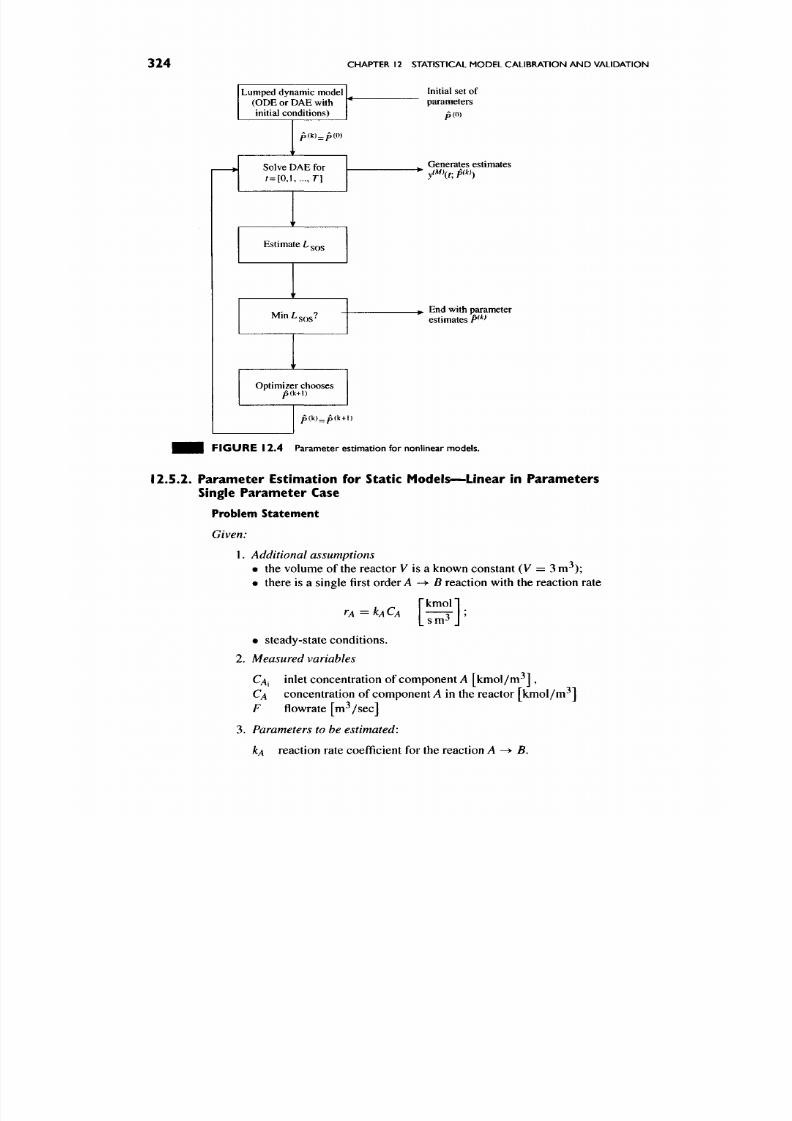
8/17/2019 Process Modelling and Model Analysis-Hangos-Cameron
http://slidepdf.com/reader/full/process-modelling-and-model-analysis-hangos-cameron 341/560
324 CHAPTER 12 STATISTICAL MODEL CALIBRATION AN D VALIDATION
Lumped dynamic model
(ODE or DAE with
initial conditions)
p(k)^p(0)
4r
Solve DAE for
r = [ 0 , l , . . . , r ]
•
Estimate L ^^
' r
MinLs^3?
>
Optimizer chooses
p(k+l)
p(k)^p(k+
1)
Initial set of
parameters
p(0)
Generates estima tes
End with parameter
estimates P^ ^
FIGURE 12 .4 Parameter estimation fo r nonlinear models.
12.5.2. Parameter Estimation for Static Models—Linear in Parameters
Single Parameter Case
Problem Statement
Given:
1. Additional assumptions
• the volume of the reactor V is a known constant (V =
3
m^);
• there is a single first order A -> B reaction w ith the reaction rate
r k m o l l
K A
= KACA —
T -
;
[sm^ J
• steady-state cond itions.
2. Measured variables
Q j inlet concentration of component A [kmol /m^] ,
CA concentration of com ponent A in the reactor [kmol/m^]
F flowrate [m ^/sec ]
3. Param eters to be
estimated:
IcA reaction rate coefficient for the reaction
A
->• 5.
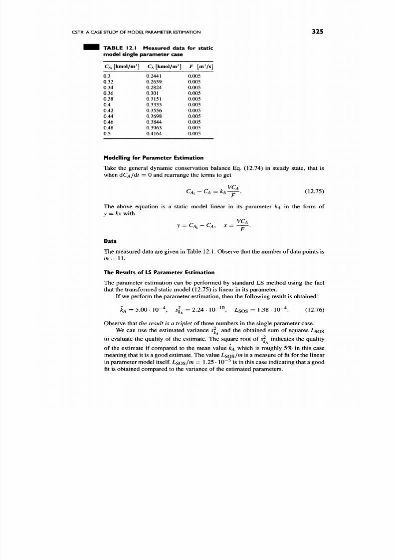
8/17/2019 Process Modelling and Model Analysis-Hangos-Cameron
http://slidepdf.com/reader/full/process-modelling-and-model-analysis-hangos-cameron 342/560
CSTR:
A
CASE STUDY OF MODEL PARAMETER ESTIMATION
325
H H TABLE 12.1 Measured data for static
model single parameter case
CA,
[kmol/m^]
0.3
0.32
0.34
0.36
0.38
0.4
0.42
0.44
0.46
0.48
0.5
C^
[kmol/m^]
0.2441
0.2659
0.2824
0.301
0.3151
0.3333
0.3556
0.3698
0.3844
0.3963
0.4164
F
[mVs]
0.005
0.005
0.005
0.005
0.005
0.005
0.005
0.005
0.005
0.005
0.005
Modelling for Parameter Estimation
Take the general dynamic conservation balance Eq. (12.74) in steady state, that is
when dC^/df = 0 and rearrange the terms to get
CA,-CA=kA-^, (12.75)
F
The above equation is a static model linear in its parameter kA in the form of
y
=
kx
with
VCA
J = Q i - C A ,
X
=
Data
The m easured data are given in Table
12.1.
Observe that the number of data points is
m = 11.
The Results of LS Parameter Estimation
The parameter estimation can be performed by standard LS method using the fact
that the transformed static mod el (12.75) is linear in its parameter.
If we perform the parameter estimation, then the following result is obtained:
JcA
=
5.00 • 10-4 ,
sj^
= 2.24 .
10"^^,
Lsos = 1 3 8
•
10 "^ . (12.76)
Observe that the result is a triplet of three numbers in the single parameter case.
We can use the estimated variance 5^ and the obtained sum of squares L sos
to evaluate the quality of the estimate. The square root of
s^
indicates the quality
of the estimate if compared to the mean value ICA which is roughly 5% in this case
meaning that it is a good estimate. The value L s o s / ^ is a measure of fit for the linear
in parameter model itself. L s o s / ^ = 1
-25
• 10 "^ is in this case indicating that a good
fit is obtained compared to the variance of the estimated parameters.
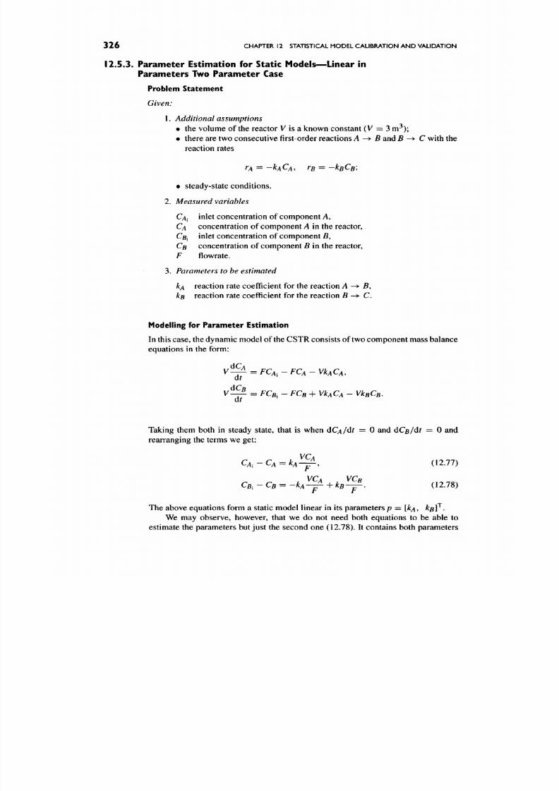
8/17/2019 Process Modelling and Model Analysis-Hangos-Cameron
http://slidepdf.com/reader/full/process-modelling-and-model-analysis-hangos-cameron 343/560
326
CHAPTER
12
STATISTICAL MODEL CALIBRATION AND VALIDATION
12.5.3. Parameter Estimation for Static Models—Linear in
Parameters Two Parameter Case
Problem Statement
Given:
1.
Additional assumptions
• the volume of the reactor V is a known con stant (V =
3
m^);
• there are two consecutive first-order reactions A -> B and B ^^ C with the
reaction rates
rA = -^ACA. rs =
-ksCB;
• steady-state cond itions.
2. Measured variables
Q j inlet concentration of component
A,
CA concentration of com ponent A in the reactor,
C j inlet concen tration of com ponent
B,
CB concentration of com ponent B in the reactor,
F
flowrate.
3. Parame ters to be estimated
kA
reaction rate coefficient for the reaction A -> 5,
ks reaction rate coefficient for the reaction B ^> C.
Modelling for Parameter Estimation
In this case, the dynamic model of the CSTR consists of two component mass balance
equations in the form:
V^=FCA,-FCA-VkACA.
V^ = FCB, - FCB +
VkACA
- VkBCB.
Taking them both in steady state, that is when dC ^/d r = 0 and dC ^/d r = 0 and
rearranging the terms we get:
VCA
CA,-CA=kA-^. {nil)
VCA VCB
CB, -CB = -kA-^+kB-^. (12.78)
F F
The above equ ations form a static model linear in its parameters
p = [kA,
^fi]^.
We may observe, however, that we do not need both equations to be able to
estimate the parameters but just the second one (12.78). It contains both parameters

8/17/2019 Process Modelling and Model Analysis-Hangos-Cameron
http://slidepdf.com/reader/full/process-modelling-and-model-analysis-hangos-cameron 344/560
CSTR:
A
CASE STUDY OF MODEL PARAMETER ESTIMATION
327
^ ^ H TABLE 12.2 Measured data for static model two param eter case
CA,[kmol/in^]
0.3
0.32
0.34
0.36
0.38
0.4
0.42
0.44
0.46
0.48
0.5
CA [kmol/m^]
0.2495
0.2638
0.2866
0.3021
0.3231
0.3273
0.3437
0.3681
0.3867
0.3987
0.4192
Cs, [kmol/m^]
0.6
0.6
0.6
0.6
0.6
0.6
0.6
0.6
0.6
0.6
0.6
CB [kmol/m^]
0.0311
0.0312
0.0313
0.0314
0.0319
0.0318
0.0322
0.0323
0.0328
0.0323
0.0329
F l m V s ]
0.005
0.005
0.005
0.005
0.005
0.005
0.005
0.005
0.005
0.005
0.005
and it is static and linear in its parameters in the form of y = p x with
J^CB^-CB,
p = {kA, ^BY , x=\——, — - .
Data
The measure data set consisting of m = 11 items is given in Table 12.2.
The Results of
LS
Parameter Estimation
The parameter estimation can be performed by standard LS method using the
transformed static model equation (12.78) which is linear in its parameters.
The LS parameter estimation results in the following data:
kA
= 5.00 . 10"^,
h
== 4.50 • 10 -2, (J2.79)
^ ^ ^ ^ ^ ^ = [ 8 . 6 2 . 1 0 - 6 9 . 2 1 . 1 0 - ^ ' ^^^-^^^
Ls os = 0.297. (12.81)
Observe that
the result is a triplet
again but now we have the vector of the estimated
parameter, its covariance matrix and the sum of squares being a scalar.
We can use the following derived quantities to assess the quality of the estim ate
and to measure the fit:
1. The empirical variances s and s to
compute their square roots and compare
them with the mean values, that is
Sk^
=
9.07 • 1 0 - ^ ,
Sks =
9.60 • 1 0 " ^
These v alues indicate that our estimate is poor as these values are higher than
the mean value of the estimate.
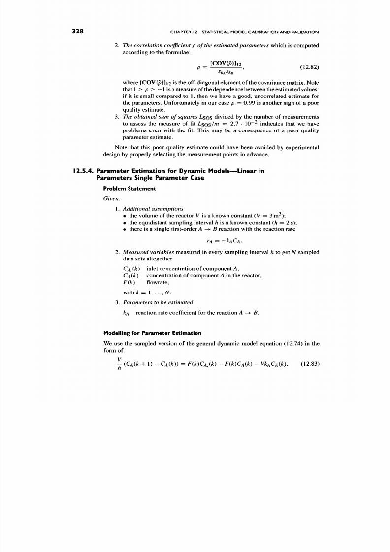
8/17/2019 Process Modelling and Model Analysis-Hangos-Cameron
http://slidepdf.com/reader/full/process-modelling-and-model-analysis-hangos-cameron 345/560
3 2 8 CHAPTER 12 STATISTICAL MODEL CALffiRATION AN D VALIDATION
2.
The correlation coefficient p of the estimated parameters
which is computed
according to the formulae:
, = £2XM 1 , ,,2.82,
where [COV{p}] 12 is the off-diagonal element of the covariance matrix. Note
tha t l
> p>
—lis a measure of the dependence between the estimated values:
if it is small compared to 1, then we have a good, uncorrected estimate for
the parameters. Unfortunately in our case
p =
0.99 is another sign of a poor
quality estimate.
3.
The obtained sum of squares
Lsos divided by the number of measurements
to assess the measu re of fit Ls os /^J = 2.7 • 10~^ indicates that we have
problems even with the fit. This may be a consequence of a poor quality
parameter estimate.
Note that this poor quality estimate could have been avoided by experimental
design by properly selecting the measurement points in advance.
12.5.4. Parameter Estimation for Dynamic Models—Linear in
Parameters Single Parameter Case
Problem Statement
Given:
1.
Additional assumptions
• the volume of the reactor V is a known constant (V = 3 m^);
• the equidistant samp ling interval ft is a known constant (h = 2 s);
• there is a single first-order
A -> B
reaction w ith the reaction rate
rA = -I^ACA-
2. Measured variables measured in every sampling interval h to get A^ sampled
data sets altogether
Q j (k ) inlet concentration of comp onent A,
C^ (k) concentration of com ponent
A
in the reactor,
F{k)
flowrate,
with A: =
1,...,A^.
3. Param eters to be estimated
IcA reaction rate coefficient for the reaction A -^ B.
Modelling for Parameter Estimation
We use the sampled version of the general dynamic model equation (12.74) in the
form of:
J (CAHC
+ 1) -
CAHC)) = F(k)CA,(k) - F{k)CA{k) - VkAC Aik).
(12.83)
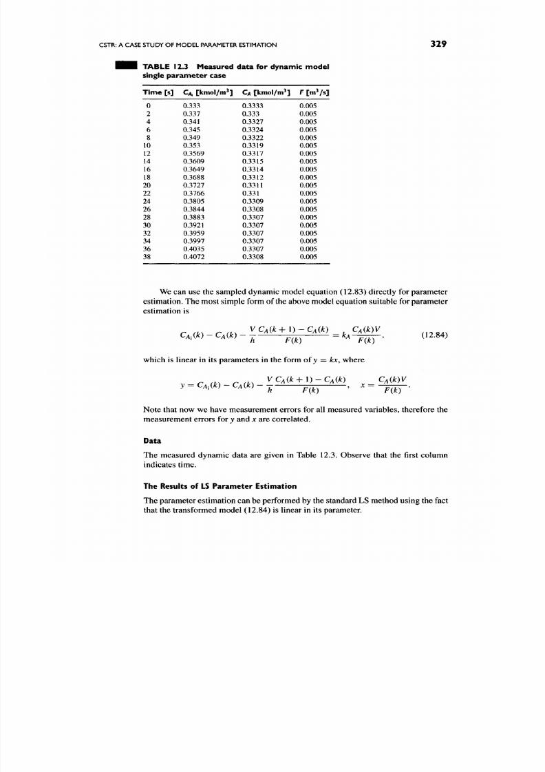
8/17/2019 Process Modelling and Model Analysis-Hangos-Cameron
http://slidepdf.com/reader/full/process-modelling-and-model-analysis-hangos-cameron 346/560
CSTR: A CASE STUDY OF MODEL PARAMETER ESTIMATION 329
TABLE
i
2.3 Measured data for dynamic model
single parameter case
Time [s ]
0
2
4
6
8
10
12
14
16
18
20
22
24
26
28
30
32
34
36
38
CA, [kmol/m^]
0.333
0.337
0.341
0.345
0.349
0.353
0.3569
0.3609
0.3649
0.3688
0.3727
0.3766
0.3805
0.3844
0.3883
0.3921
0.3959
0.3997
0.4035
0.4072
CA [kmo /m^]
0.3333
0.333
0.3327
0.3324
0.3322
0.3319
0.3317
0.3315
0.3314
0.3312
0.3311
0.331
0.3309
0.3308
0.3307
0.3307
0.3307
0.3307
0.3307
0.3308
F [mVs]
0.005
0.005
0.005
0.005
0.005
0.005
0.005
0.005
0.005
0.005
0.005
0.005
0.005
0.005
0.005
0.005
0.005
0.005
0.005
0.005
We
can use the sampled dynamic model equation (12.83) directly for parameter
estimation. The most simple form of the above model equation suitable for parameter
estimation is
Q,(/:)
- cm - — ^ = k,-j^, (12.84)
which is linear in its parameters in the form o iy
—
kx, where
^ , , , ^ , . , V Q ( f e + l ) - Q « : ) Q(fe)V
y^c^^k)~cm--^
— ^
, ^ --FoT-
Note that now we have measurement errors for all measured variables, therefore the
measurement errors for y and x are correlated.
Data
The measured dynamic data are given in Table 12.3. Observe that the first column
indicates time.
The Results of LS Parameter Estimation
The parameter estimation can be performed by the standard LS method using the fact
that the transformed model (12.84) is linear in its parameter.

8/17/2019 Process Modelling and Model Analysis-Hangos-Cameron
http://slidepdf.com/reader/full/process-modelling-and-model-analysis-hangos-cameron 347/560
3 3 0 CHAPTER 12 STATISTICAL MODEL CALIBRATION AN D VALIDATION
The LS parameter estimate gives the following result:
kA
= 5.00 • 10"^ ,
sj^ =
1.20 . 10~^^, L so s = 1.17 • 1 0 " ^ (12.85)
The results can be compared to the similar ones obtained for the same CSTR
but using its static model and steady-state data given in Eq. (12.76). Comparing the
correspond ing elem ents in the two results, we come to the conclusion that the quality
of the estimate is roughly the same for the dynamic and the static case.
12.6. STATISTICAL MODEL VALIDATION VIA PARAMETER ESTIMATION
The
principle of statistical model
validation is to compare by the methods of
mathematical statistics either
• the (measured) system output with the model output, or
• the estimated system parameters with the model param eters.
In other words "validation" means "comparison" of
{y
and
J M )
or
(p
and
PM)-
Statistical methods are needed because the measured output y is corrupted by
measurement (observation) errors
y
= J W +
8.
As was emphasized in Section 12.1.2 on model calibration, model validation is
similar to model calibration because here we also use measured data, but another,
independendy measured data set
(validation data)
and also use statistical methods.
The items of the instance of a m odel validation problem are as follows:
• a developed and calibrated
process model,
• measured data from the real process system which we call validation data,
•
a predefined measure of fit, or
loss function
which m easures the quality of the
process model with its missing parame ters and/or structure elements estimated.
The conceptual steps to be carried out when performing model validation are
also similar to that of m odel calibration and include:
1.
Analysis of the process mod el
This step m ay involve the analysis of the uncertainties in the calibrated proces s
model and its sensitivity analysis. The results can be applied for designing
experiments for the model validation.
2. Sampling of continuous time dynamic models
As before in model calibration.
3. Data analysis and preprocessing
As before in model calibration. (The methods for this are described in
Section 11.2.)
4.
Mode l parameter a nd structure estimation

8/17/2019 Process Modelling and Model Analysis-Hangos-Cameron
http://slidepdf.com/reader/full/process-modelling-and-model-analysis-hangos-cameron 348/560
REVIEW QUESTIONS 331
5. Evaluation of the quality
The evaluation is done by using either empirical graphica l method s or by exact
hypothesis testing if the mathematical statistical properties of the estimates
are available. More d etails are given abou t the measure of fit in Section 12.3.
In order to perform statistical model validation, we need to be able to solve the
following mathematical problems.
1. Hy pothesis testing in case of
• steady-state hypothesis for single and multiple variables,
• comparing step responses.
2. Parameter estimation in most of the cases for the linear in parameters case
together with hypothesis testing on the estimated parameters.
12.7.
SUMMARY
Basic methods and procedures for statistical model calibration and validation are
included in this chapter based on a grey-box modelling approach.
The basic technique we use for model calibration and validation is model para
meter and structure estimation for both static and dynamic m odels. The procedure for
model param eter estimation together with the analysis of the distribution and statistics
of the estimated parameters has been covered. The way of constructing confidence
intervals and methods for assessing the fit have also been discussed.
12.8.
FURTHER READING
The tools and techniques of model calibration and validation are not just for pro
cess models but for dynamic models of any kind. The origin of the techniques is in
mathematical statistics and in systems and control theory under the name of "identi
fication". Therefore, further reading is recommended in both of the above mentioned
fields.
A recent and excellent review on model validation and model error modelling
can be found in the technical report [85] which is available through the Web using
the address h t t p : / / w w w . c o n t r o l . i s y . l i u . s e .
There are several special books and monographs available about parameter
estimation in process systems such as [86-8 8].
12.9.
REVIEW QUESTIONS
Q12.1. What is the difference between the
black-box, grey-box
and
white-box
models of the same process system. Illustrate your answer on the Example 12.1.1
in Section 12.1.
Q12.2. W hat are the statistical properties of the estimated param eters obtained by LS
estimation for models linear in parameters and with Gaussian independent measure
ment errors? How c an we construct confidence intervals for the individual parameters
and how these intervals relate to the joint confidence region of the parameters?
(Section 12.2.2)
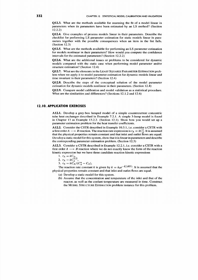
8/17/2019 Process Modelling and Model Analysis-Hangos-Cameron
http://slidepdf.com/reader/full/process-modelling-and-model-analysis-hangos-cameron 349/560
3 3 2 CHAPTER 12 STATISTICAL MODEL CALIBRATION AN D VALIDATION
Q12.3. What are the method s available for assessing the fit of a model linear in
parameters when its parameters have been estimated by an LS method? (Section
12.2.2)
Q12.4. Give examp les of process models linear in their parameters. Desc ribe the
checklist for performing LS parameter estimation for static models linear in para
meters together with the possible consequences when an item in the list fails.
(Section 12.3)
Q12.5. What are the methods available for performing an LS parameter estimation
for models nonlinear in their parameters? How would you compute the confidence
intervals for the estimated p arameters? (Sec tion 12.2.2)
Q12.6. What are the additional issues or problems to be considered for dynamic
models compared with the static case when performing model parameter and/or
structure estimation? (Section 12.4)
Q12.7. What
are
the elements in the
LEAST SQUARES PARAMETER ESTIMATION
prob
lem when we apply it to model parameter estimation for dynamic models linear and
time invariant in their parameters? (Section 12.4)
Q12.8. Describe the steps of the conceptual solution of the model parameter
estimation for dynamic models nonlinear in their parameters. (Section 12.4)
Q12.9, Com pare model calibration and model validation as a statistical procedure.
Wh at are the similarities and differences? (Sections 12.1.2 and 12.6)
12.10.
APPLICATION EXERCISES
A12.1. Develop a grey-box lumped mod el of a simple countercurrent concen tric
tube heat exchanger described in Example 7.2.1. A simple 3-lump model is found
in Chapter 13 as Example 13.2.2. (Section 12.1). Show how you would set up a
parameter estimation problem for the heat transfer coefficients.
A12.2.
Consider the CSTR described in Example 10.3.1, i.e. consider a CSTR with
a first order A —
y B
reaction. The reaction rate expression is r^ = kCJ^. It is assumed
that the physical properties remain constant and that inlet and ou det flows are equal.
Develop a static model for this system, show that it is linear in param eters and describe
the corresponding parameter estimation problem. (Section 12.3)
A12.3.
Consider a CSTR described in Example 12.2.1, i.e. consider a CSTR with a
first order
A
—
> B
reaction where we do not exactly know the form of the reaction
kinetic expression but we have three candidate reaction kinetic expressions
1. VA =kCA,
2.
rA
= kc\^\
3. r ^ = / c Q / ( C * - Q ) ,
The reaction rate constant k is given hy k = koQ~^^^^^\ It is assumed that the
physical properties remain constant and that inlet and outlet flows are equal.
(a) Develop a static model for this system.
(b) Assume that the concentration and temperature of the inlet and that of the
reactor, as well as the coolant temperature are measured in time. Construct
the MO DEL STRUCTURE ESTIMATION problem instance for this problem.
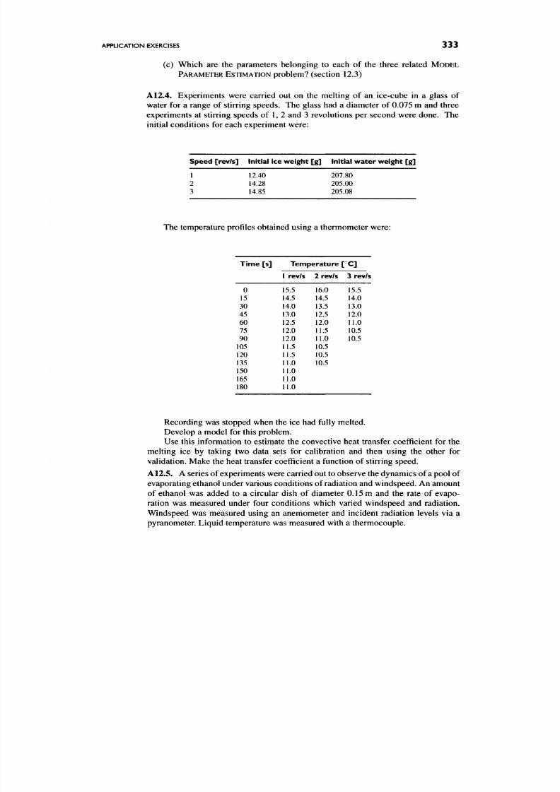
8/17/2019 Process Modelling and Model Analysis-Hangos-Cameron
http://slidepdf.com/reader/full/process-modelling-and-model-analysis-hangos-cameron 350/560
APPLICATION EXERCISES
333
(c) Which are the parameters belonging to each of the three related M O D E L
PARAMETER ESTIMATION problem? (section 12.3)
A12.4. Exp eriments were carried out on the melting of an ice-cube in a glass of
water for a range of stirring spe eds. The glass had a diameter of
0.075
m and three
experime nts at stirring speeds of 1, 2 and 3 revolutions per second were done . The
initial conditions for each experiment were:
Speed [rev/s] Initial ice weight [g ] Initial water weight [g ]
1 12.40 207.80
2 14.28 205.00
3 14.85 205.08
The temperature profiles obtained using a thermometer were:
Time [ s ]
0
15
30
45
60
75
90
105
120
135
150
165
180
Temperature
1 rev/s
15.5
14.5
14.0
13.0
12.5
12.0
12.0
11.5
11.5
11.0
11.0
11.0
11.0
2 rev/s
16.0
14.5
13.5
12.5
12.0
11.5
11.0
10.5
10.5
10.5
rc]
3 rev/s
15.5
14.0
13.0
12.0
11.0
10.5
10.5
Recording was stopped when the ice had fully melted.
Develop a model for this problem.
Use this information to estimate the convective heat transfer coefficient for the
melting ice by taking two data sets for calibration and then using the other for
validation. Make the heat transfer coefficient a function of stirring speed.
A12.5.
A series of experim ents were carried out to observe the dynamics of a pool of
evaporating ethanol under various conditions of radiation and windspeed. An amount
of ethanol was added to a circular dish of diameter 0.15 m and the rate of evapo
ration was measured under four conditions which varied windspeed and radiation.
Windspeed was measured using an anemometer and incident radiation levels via a
pyranometer. Liquid temperature was measured with a thermocouple.
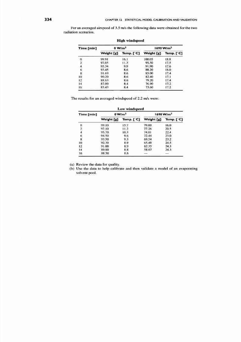
8/17/2019 Process Modelling and Model Analysis-Hangos-Cameron
http://slidepdf.com/reader/full/process-modelling-and-model-analysis-hangos-cameron 351/560
334
CHAPTER 12 STATISTICAL MODEL CALIBRATION A ND VA LIDATION
For an averaged airspeed of 3.5 m/s the following data w ere obtained for the two
radiation scenarios.
High windspeed
Time [min]
0
2
4
6
8
10
12
14
16
OW/m^
Weight [g] Temp. [ C]
99.91
97.05
95.34
93.45
91.69
90.20
88.63
87.00
85.43
16.1
11.3
9.9
8.6
8.6
8.6
8.6
8.4
8.4
l 6 9 0 W /m^
Weight [g]
100.05
95.50
91.90
88.20
85.00
82.40
79.20
76.90
73.60
Temp.
[ C ]
18.8
17.5
17.6
18.0
17.4
17.1
17.4
17.2
17.2
The results for an averaged windspeed of 2.2 m/s were:
Low windspeed
Time [mm]
0
2
4
6
8
10
12
14
16
OW/m^
Weight [g ] Temp. [ X ]
99.10
97.10
95.70
94.50
93.50
92.30
91.00
89.80
88.50
15.7
11.2
10.3
9.6
9.3
8.9
8.9
8.8
8.6
l 6 9 0 W /m^
Weight [g]
79.00
77.26
74.81
72.44
69.54
65.48
62.35
58.07
—
Temp. [-C]
16.0
20.5
22.4
23.0
23.2
24.5
24.3
24.3
—
(a) Review the data for quality.
(b) Use the data to help calibrate and then validate a model of an evaporating
solvent pool.
8/17/2019 Process Modelling and Model Analysis-Hangos-Cameron
http://slidepdf.com/reader/full/process-modelling-and-model-analysis-hangos-cameron 352/560
ANALYSIS
OF
DYNAMIC
PROCESS MODELS
Lumped dynamic process models form an important class of process models. They
are in the form of DAE systems with given initial conditions. Their main application
area is process control and diagnosis where they are the models which are almost
extensively used.
This chapter deals with the analysis of various dynamical system properties
relevant to process control and diagnosis applications. Therefore, only lumped para
meter process models are treated throughout the chapter. Analytical as well as
structural approaches and techniques are described.
The material presented in this chapter contains basic material for analysing
dynam ical properties w hich can then be used as model verification tools. The m aterial
is arranged in sections as follows:
• The design of mo del-based control and diagnostic method s usually starts with
analysis of system properties. Therefore, the initial section covers the basic
notions and most important analysis methods for stability, controllability and
observability (Section 13.1).
• Section 13.2 deals with the analysis of structural control properties, w hich
are dynamical properties valid for a class of process systems with the same
structure.
• Dyn amic process mo dels for control and diagnostic purpose s should be rel
atively simple, containing only a few state variables. Therefore, model
simplification and reduction play
a
key role. This is the subject of Section 13.3.
335
8/17/2019 Process Modelling and Model Analysis-Hangos-Cameron
http://slidepdf.com/reader/full/process-modelling-and-model-analysis-hangos-cameron 353/560
336 CHAPTER 13 ANALYSIS O F DYNAMIC PROCESS MODELS
13.1 .
ANALYSIS
OF
BASIC DYNAMICAL PROPERTIES: CONTROLLABILITY,
OBSERVABILITY
AND
STABILITY
This section deals with the basic dynam ic system prop erties of controllability, observ
ability and stability. These properties are introduced for the general nonlinear SSR in
the form of:
i = / ( x , w ) , y = g{x,u), (13.1)
where / and
g
are given no nlinear functions.
Conditions to check controllability, observability and stability will be given for
LTI systems with finite-dimensional representations in the form:
JC
=
AJC
+ BW, J = CJC. (13.2)
Observe that from now on we assume D = 0 in the general form of the SSR in
Eq. (13.2). Therefore, a SSR will be characterized by the triplet (A, B, C). Note also
that SSRs are not unique: there is infinitely many equivalent SSRs g iving rise to the
same input-output behaviour as shown in Section 10.2.2.
13.1.1. State Observability
The state variables of a system are no t directly observable. Therefore, we need to
determine the value of the state variables at any given time from the measured inputs
and outputs in such a way that w e only use functions of inputs and outputs and their
derivatives together with the known system model and its parameters. We need to
be able to perform this task if we want to control the states or if we want to operate
a diagnostic system based on the value of state variables. A system is called (state)
observable, if from a given finite m easurement record of he input and output variables,
the state variable can be reconstructed at any given time.
The problem statement of state observability can be formalized as follows:
STATE OBSERVABILITY
Given:
The form of the SSR (13.1) together with its parameters and a measurement record
for inputs and outputs
V[t^. T] = {M(r), y(T) \to<T<T]. (13.3)
Question:
Is it possible to determine u niquely the value of the state variable
x{to)l
Note that it is sufficient to determine the value of the state variable at a given
time instance because the solution of the state equation (13.1) gives us the state at
any other time instance.
LTI systems
In the case of LTI systems, the SSR matrices (A, B, C) are sufficient and enough to
specify a given system .

8/17/2019 Process Modelling and Model Analysis-Hangos-Cameron
http://slidepdf.com/reader/full/process-modelling-and-model-analysis-hangos-cameron 354/560
ANALYSIS OF BASIC DYNAMICAL PROPERTIES
337
An LTI system may or may not be
state observable,
meaning that the problem
above does not always have a unique solution for every (A, B, C). The following
theorem gives necessary and sufficient conditions for an LTI system to be state
observable.
THEOREM 13.1.1. Given
an
LTI with
its
SSR (A, B,C). This SS R with state space
X is
state observable
if and only if the
observability matrix
On is of full rank
On =
C
CA
CA
n-l
(13.4)
that is
rank
On = n,
where
dim
X = n is the dimension of the state vector
Note that
(state) observability
is
a realization property
and therefore does depend
on the realization because the rank of the observability matrix may change if we
perform any transformation of the SSR. See Eq. (10.30) for this condition.
EXAMPLE 13.1.1 (Observability matrix of a linearized CST R mod el). Derive
the observability matrix of the linearized CSTR model described in Examples 10.3.1
and 10.4.5 considering only the coolant temperature TQ as input and the con centration
of component A ( Q ) as output.
The symbolic form of the state space model matrices can be obtained from the
matrices (10.114) by omitting the first column from B and the last row from C:
kj-
Using these matrices the observability matrix in symbolic form is
0 ^ \ ' M . (13.6)
[ - a i l - « 1 2 J
It is seen that
O
is of full rank and is a square matrix because there is only one input
• variable (r = 1).
There are ready and easy-to-use procedures in MATLAB to compute the observ
ability m atrix of an LTI system w ith realization (A, B, C) ( o b s v ) and check its rank
( r a n k ) . Their use is illustrated by the following example.
• EXAMPLE 13.1.2 (Observability matrix of simple SISO LTI mo del). Derive
the observability matrix of the simple LTI SISO model described in Example
10.2.1.
The observab ility m atrix will be a square m atrix because we have a SISO system.
We can use the MATLAB procedure ob = o b s v (A, C) to obtain
O b
^

8/17/2019 Process Modelling and Model Analysis-Hangos-Cameron
http://slidepdf.com/reader/full/process-modelling-and-model-analysis-hangos-cameron 355/560
[1
0
0
[5
O l
1
0
- 7
338
CHAPTER 13 ANALYSIS OF DYN AMI C PROCESS MODELS
Observe the presence of the output matrix C in the first block being the first row of
the observability matrix.
The observability matrix above has rank 2 compu ted by the MATL AB procedure
• • • r a n k (o b ), therefore the system is observable.
The following simple example illustrates the case when we have two outputs and
an unstable system.
• • • EXAMPLE 13.1.3 (Observability matrix of simple MIM O LTI model). Derive
the observability m atrix of the following u nstable LTI MIMO model specified by its
state space realization matrices (A, B, C):
The ob servability m atrix is a 4 x 2 matrix this time with the input matrix in its first
block:
O
Its rank is now 2 due to the full rank upper block being the output matrix C which
ensures observability even when the state matrix A and therefore the second block
CA in the observability matrix has rank 1.
13.1.2. State Controllability
For process control pu rposes over a wide operation ran ge, we need to drive a process
system from its given initial state to a specified final state. A system is called
(state)
controllable if we can always find an appropriate man ipulable input function which
moves the system from its given initial state to a specified final state in finite time.
This applies for every given initial state final state pair.
The problem statement of state controllability can be formalized for LTI systems
as follows:
STATE CONTROLLABILITY
Given:
The SSR form with its parameters as in Eq. (13.1) and the initial x{t\) and final
x(t2) ^ x(t\)
states respectively.
Question:
Is it possible to drive the system from
x(t\)
to
x{t2)
in finite time?
LTI systems
For LTI systems there is a necessary and sufficient condition for state controllability
which is stated in the following theorem.
THEOREM 13.1.2.
A SSR
(A, B, C)
is state controllable if and only if the
controllability matrix C:
Cn= [B AB . . . A" -^B ] (13.7)
8/17/2019 Process Modelling and Model Analysis-Hangos-Cameron
http://slidepdf.com/reader/full/process-modelling-and-model-analysis-hangos-cameron 356/560
ANALYSIS OF BASIC DYNAMICAL PROPERTIES
339
is of full
rank,
that is
rank
Cn
= n.
Note again that controllability is a realization property, and it may change if
we apply state transformations to the SSR.
Joint controllability and observability,
however, is a system property being invariant under state transformations of SSR.
The following example illustrates the computation of the controllability matrix.
• • • EXAMPLE 13.1.4 (Controllability matrix of
a
linearized CST R mo del). Derive
the controllability matrix of the linearized CSTR model described in Examples
10.3.1 and 10.4.5 by considering only the coolant temperature TQ as input and the
concentration of com ponent
A (CA)
as o utput.
The sym bolic form of the state space model matrices for this case has been derived
in Example 13.1.1. With the matrices (13.5) the following observability m atrix results:
[bzi
- 22^22]
*
It is seen that C is of full rank and it is a square matrix because there is only one
output variable
(m =
1).
There are ready and easy-to-use procedures in MATLAB to compute the con
trollability m atrix of an LTI system w ith realization (A, B, C) ( c t r b ) and check its
rank (rank). Their use is illustrated by the following example.
EXAMPLE 13.1.5 (Controllability matrix of simple SISO LTI mo del). Derive
the controllability matrix of the simple LTI SISO m odel described in Exam ple
10.2.1.
The con trollability m atrix will be a square matrix because w e have
a
SISO system.
We can use the MATLAB procedure c o = c t r b ( A , C ) to obtain
C O
- [ 8 - B J -
Obse rve the presenc e of the input matrix B in the first block being the first column of
the controllability matrix.
The controllability matrix above has rank 2 (computed by the MATLAB
• • • procedure r a n k ( c o )) , therefore the system is controllable.
The following simple example illustrates the case when we have two inputs and an
unstable system.
• • • EXAMPLE 13. L6 (Controllability matrix of a simple MIS O LTI
model).
Derive
the controllability m atrix of the simple LTI MISO model described in Exam ple 10.2.3.
The controllability m atrix is now a 2 x 4 matrix with the 2 x 2 input matrix B in
its first block:
_ [7 0 - 2 8 24 1
~ [o 8 35 - 4 8 ] •
Its rank is 2, therefore the system is controllable. Observe that if the input matrix B
is of full rank in this case then the state matrix "cannot destroy" controllability.
8/17/2019 Process Modelling and Model Analysis-Hangos-Cameron
http://slidepdf.com/reader/full/process-modelling-and-model-analysis-hangos-cameron 357/560
340 CHAPTER 13 ANALYSIS OF DYN AMI C PROCESS MODELS
13.1.3. Asymptotic and Bounded Input Bounded Output Stability
There are two related but different kinds of stability w e investigate:
• BIBO stability which is also known as external stability,
• asym ptotic stability, known as internal stability.
They are defined for both SISO and MIMO systems. In the case of LTI systems
there are necessary and sufficient conditions to check both kinds of stability [70].
BIBO Stability
The system is BIBO or externally stable if it responds to any bounded-input signal
with a bounded-output signal. Hence, for any
{||M(OII < M i < o o | - r < r < 00} =^ {||j(OII < M2 < o o | - T < r < oo},
(13.9)
where || • || is a suitable vector norm and M \, M2 are constan ts. For more about vector
and signal norms refer to Section A.3 in Appendix A.
BIBO stability is clearly a system property. If we consider the system represented
by its input-output operator S then the definition in Eq. (13.9) can be reformulated
to have
||S|| < 5 M < 00,
where || • || is the so-called induced operator norm of the system operator induced by
the signal norms app lied for u and y.
Note that the definition above says nothing about the states. The variation of
the state variables may or may not be bounded, given a bounded input signal to the
system.
LTI systems
For SISO LTI systems there is a necessary and sufficient condition for BIB O stability.
LEMMA 13.1.1. An SISO LTI system is BIBO or externally stable if and only if
r»oo
\h(t)\dt<M
< o o , (13.10)
Jo
o
where M is a constant and h(t) is the impulse response function of the system.
Asymptotic or Internal Stability
A solution to the state equation of a system is asymptotically stable if a "neighbouring"
solution, resulting from a perturbation and described by a different initial condition
has the same limit as r -> 00. The following defining co nditions formulate the above
in a rigorous mathematical way.
Consider a nonlinear lumped parameter system described by the state space
model in Eq. (13.1) with the initial condition for the state vector ^(0) =
XQ
giving
rise to the nominal solution
x^(t),
t < 0. The nominal solution of the system is
asymptotically stable if whenever we take another different initial condition
XQ
such
that ||jco
—
XQW
< 8
with
8 > 0
being sufficiently small, then
| | j c (0-Jc^(OI | ->0 i f r ->cx) ,

8/17/2019 Process Modelling and Model Analysis-Hangos-Cameron
http://slidepdf.com/reader/full/process-modelling-and-model-analysis-hangos-cameron 358/560
ANALYSIS
O F
STRUCTURAL DYNAMICAL PROPERTIES 341
where || • || is a vector norm and
x(t),
r < 0 is the
perturbed solution
with initial
condition A:(0) = XQ.
LTI systems
Unlike nonlinear systems which may have stable and unstable solutions
stability
is a system property for LTI systems. An LTI system with realization (A, B, C) is
asymptotically or internally stable
if
the
solution
x(t)
of the truncated state equation:
x(t) =
AJC(0, ^(^O) = JCO 7^ 0,
t > to (13.11)
satisfies
lim x{t)=0, (13.12)
We usually omit the word "asy mp totic" from asymp totic stability if it does not create
any confusion. We call a system "stable" if it is asymptotically stable.
Note that the above condition is similar to asymptotic stability of linear ODEs.
The notion has app eared first in the context of analysing num erical stability of O DEs
and DAEs in Section 5.11.5.
There is an easy-to-check necessary and sufficient condition for asymptotic
stability of LTI systems.
THEOREM 13.1.3. An LTI system is internally stable if and only if all of the
eigenvalues,
A/(A)
of the state matrix
A
have strictly negative
real
parts:
Re{A./(A)} < 0, V/.
Again, note that the eigenvalues of the state matrix remain unchanged by state
transformations, and hence
stability is indeed a system property for LTI systems.
The following simple examples illustrate how one can use MATLAB to check
stability of LTI systems.
• • • EXAMPLE 13. L7 (Stability of a simple SISO LTI system ). Check the asymp
totic stability of the simple LTI SISO system described in Example 10.2.1.
The eigenvalues of the state matrix
A are
com puted using
the
MATLAB procedure
e i g (A) to obtain —1, —9. This shows that the system is asymptotically stable.
The stability of the system implies that the unit step response function will
• • • converge to a finite value as time goes to infinity. This is seen in Fig. 10.4.
Wmm
EXAMPLE
13.
L8
(Stability of a simple MIS O LTI system). Check the asymp
totic stability of the simple LTI MISO system described in Example 10.2.3.
The eigenvalues of the state matrix A are —6,0. This means that the system is
no t
asymptotically stable.
If we have an unstable system then we cannot expect the unit step response
computed with respect to any input by s t e p (A, B , C, D, i ) to converge to a finite
• • • value. This is seen in Fig. 10.6 of the unit step for the first { i = 1) input variable U{.
13.2. ANALYSIS OF STRUCTURAL DYNAMICAL PROPERTIES
As it has been described in Section 10.5.1 the structure of a linear or linearized state
space model is given in terms of its structure indices and its (signed) structure state
8/17/2019 Process Modelling and Model Analysis-Hangos-Cameron
http://slidepdf.com/reader/full/process-modelling-and-model-analysis-hangos-cameron 359/560
342 CHAPTER 13 ANALYSIS OF DYNAM IC PROCESS MODELS
space model matrices ({A}, {B}, {C}). In this way a
class ofLTI state space models
can be specified w here the mem bers in the class possess the sam e structure. If every
mem ber in the class, with the exception of
a
null measure set, has a dynam ical system
property, such as stability, controllability or observability, then w e say that the class
with
the
given structure has this
structural property.
We
call
these properties
structural
stability, controllability or observability
respectively.
In some important
cases,
the presence of structural properties is the consequ ence
of the phenomena taking place in the process system. This structural property, say
structural stability, is then guaranteed for the class of systems defined by the phen om
ena. This mea ns, that stability ho lds for any memb er of the class irrespectively of the
equipment sizes, variations in the flowsheet, etc. We shall see examples of this in the
subsequent subsections.
Because the structure of the process system depends mainly on the flowsheet
and on the phenomena taking place, simple combinatorial methods are available to
check structural properties, such as finding directed paths in a graph or com puting the
structural rank of a structure matrix. This m akes it easy to analyse structural properties
even in the early phases of process design.
The presence of a structural property in a class of process systems implies that
the property holds for the members of the class but the presence of the property in
a member of the class does not guarantee that property for the whole class. This
mean s, that one may fail to show a structural property for a class, despite the fact that
most m embers of the class may have this property. For examp le, continuously stirred
chemical reactors (CSTRs) are not always stable, therefore we will fail to show that
structural stability holds for this class of systems. But there are many CSTRs which
are stable.
13.2.1 • Structural Rank of the State Structure Matrix
The notion of structural rank of a structure matrix is similar to that of other structural
properties. If almost every m atrix of the same structure has rank n, then the structural
rank of the structure m atrix is equal to n. In other words, structural rank is the maximal
possible rank within the class specified by the structure m atrix.
The determination of the structural rank of a matrix is easy and uses the following
property: if one can find an assignment or matching of the rows and columns deter
mined by a non-zero entry in the structure m atrix then the matrix is of full structural
rank, otherwise it is the size of the maximal m atching. O ne can find computationally
easy algorithms to determine the structural rank of a structure matrix.
The following simple example high lights the relation between the structural rank
of a structure matrix and the rank of a matrix with the same structure matrix.
• • • EXAMPLE 13.2.1 (Relation between structural rank and rank of matrices).
Consider the following structure matrix Q
[ Q ] -
X 0 0 jc 0
0 x 0 0 0
jc 0 0 jc 0
0 0 jc 0 0
The underlined structurally non-zero elements x show a matching between rows and
columns and indicate that
s
— rank([Q]) = 4.
8/17/2019 Process Modelling and Model Analysis-Hangos-Cameron
http://slidepdf.com/reader/full/process-modelling-and-model-analysis-hangos-cameron 360/560
ANALYSIS OF STRUCTURAL DYNAMICAL PROPERTIES 343
If, however, we take a special numerical matrix Q from the class determined by
[Q] (that is with the same structure):
[Q] =
1 0 0 2 0
0 2 0 0 0
1 0 0 2 0
0 0 5 0 0
then its rank will be smaller, actually ran k(Q ) = 3. This is caused by the fact that the
4th column is twice the first. That is these two columns are linearly dependent.
Process systems whose dynamic state space model has originated from lumped
dynamic models have an interesting and important special structural property which
is stated below.
THEOREM 13.2.1. The state structure matrix of a process system with convective
or transfer outflow derived from lumped dynam ic process models is of full structural
rank.
This fact is a consequence of the presence of the output convective terms in the
conservation b alance equations for the quantity which appears as a nonzero (negative)
diagonal term in the linearized state equation. As none of the volumes is isolated
from the others, all of them have both in- and outflows which are either convective or
diffusive.
The general forms of a convective outflow in extensive variable form for the
volume-specific extensive quantity cp is in the form of — F^^^cp. T his can be seen from
Eq. (5.52) in Section 5.6. This term leads to the element —F^^^ if one derives the
right-hand sides of
Eq.
(5.52) to get the linearized model as is shown in Section 10.4.
The analysis of structural dynam ical properties w ill be illustrated on the exam ple
of heat exchangers and heat exchanger networks. For this purpose, the structure
matrices of a countercurrent heat exchanger are given below.
EXAMPLE 13.2.2 (Linear model structure of a heat exchan ger).
Process system
Consider a countercurrent heat exchanger where the cold liquid stream is being
heated by a hot liquid stream. The system is very similar to the one described in
Example
7.2.1.
Modelling goal
Describe the lumped linearized model structure of the heat exchanger for structural
dynamic analysis purposes.
Assumptions
v41. The overall mass (volume) of the liquids on both sides is constant.
A2. No diffusion takes place.
A3. No heat loss to the surroundings.
A4. Heat transfer coefficients a re constant.
v45. Specific heats and densities are constan t.
A6.
Both liquids are in plug flow .
Al.
The heat exchang er is described as a sequence of three CSTR pairs of hot
and cold liquid volumes.

8/17/2019 Process Modelling and Model Analysis-Hangos-Cameron
http://slidepdf.com/reader/full/process-modelling-and-model-analysis-hangos-cameron 361/560
344
CHAPTER 13 ANALYSIS OF DYN AM IC PROCESS MODELS
Balance volumes
We consider three perfectly mixed balance volumes with equal holdups for each of
the hot and cold sides.
Model equations
Variables
( r ^ ^ \ 0 , T^c^^O, ^ = 1,2,3), 0 < r ,
(13.13)
(k) (k)
where T^ (r) and T (t ) is the hot and the cold side temperature in the kih tank pair
respectively, and t is time.
Energy balances for the hot side
d r
ik)
df
^Ph^h
^ = 1,2,3,
Tl^^\t) =
Tl^\t).
T^^
is the hot liquid inlet temperature to the heat exch anger.
Energy balances for the cold side
(13.14)
(13.15)
dr ,
k)
dt
Ak)
( '
.(*+ )
>k)\ _
K^'^^A^''^
(j,(k) j,{k)\
^' ) r^)jk)ym
V< ^
'h )
Cpc^c
^ = 1 , 2 , 3 ,
T^^\t)
= T^\t).
(13.16)
(13.17)
Tc is the cold liquid inlet temperature to the heat
exchanger.
Note that the cold stream
flows in the direction of descending volume indices.
Initial conditions
T'h^^W
=f\^\
l t =
1,2,3, (13.18)
(13.19)
^''\0)=f^''\ k= 1,2,3,
(k) (k)
where the values of /j , ^ = 1, 2, 3 and /2 , k — 1, 2, 3 are g iven.
Signed state structure matrix
Note that all the model parameters are positive in the model above and the balance
equations (13.14)-(13.15) and (13.16)-(13.17) are the state equations of the linear
state space model, therefore,
{A}HE
—
+
+
0
0
0
+
-
0
0
0
0
0
0
-
+
+
0
0
+
+
—
0
0
0
0
0
0
—
+
0
0
0
+
+
—
(13.20)
8/17/2019 Process Modelling and Model Analysis-Hangos-Cameron
http://slidepdf.com/reader/full/process-modelling-and-model-analysis-hangos-cameron 362/560
ANALYSIS OF STRUCTURAL DYNAMICAL PROPERTIES
345
with the state vector
XHE
= [T^^\ T ^^\ T^\ TP, TI^\ T^^ f. (13.21)
Note that the structure graph of a heat exchanger is shown in Fig. A.3 in Section
• • • A.5 in the append ix.
It is important to note that
1.
The state structure matrix of the countercurrent heat exchanger is indeed of
full structural rank because we can easily find an assignment of the columns
and rows along the main diagonal.
2. The diagonal eleme nts of the state structure matrix (13.20) are all negative
whereas the off-diagonal elements are either positive or
zero. This property
will be impo rtant later on when analysing structural stability of co untercurrent
heat exchangers.
3. Observe the diagonal blocks belonging to a volume pair connected by a
heat conducting wall.
The connection is the consequence of the heat transfer
between them.
4.
The other positive off-diagonal elements not belonging to the diagonal blocks
indicate connections. It is easy to construct an algorithm w hich generates the
off-diagonal connection elem ents from the topology of the volume pairs and
their connections.
A simple example of three jacketted CSTRs in series further illustrates the use
of structure graphs to determine the structural rank of the state matrix.
• • • EXAMPLE 13.2.3 (Structural rank of the state matrix of the three jacketted CSTR
in series) (Exam ple 10.3.2 continu ed).
The structure graph of the three jacketted CSTR has already been developed in
Chapter 10 and is shown in Fig. 10.9. Figure 10.9 shows that there is a self-loop
adjacent to each state variable vertex, that is the state structure matrix [A] is of full
• • • structural rank.
13.2.2.
Structural Controllability and Observability
If only the structure of the system is given, then the notion of
structural contro
llability or observability
is used for ensuring that
all
systems with the given structure
are controllable or observable. These properties can be checked using the following
important result.
THEOREM 13.2.2. [7 1] A linear system with structure matrices ([A ], [B], [C]) i s
structurally controllable or observable if
1. the matrix [A] is of full structura l
rank,
and
2.
the system structure graph S is input connectable or output connectable. For
controllability there should be at least one directed path from any of the input
variables to each of the state variables. F or observability there should be at
least one directed path from each of the state variables to one of the output
variables.
8/17/2019 Process Modelling and Model Analysis-Hangos-Cameron
http://slidepdf.com/reader/full/process-modelling-and-model-analysis-hangos-cameron 363/560
346 CHAPTER 13 ANALYSIS OF DYNAMIC PROCESS MODELS
As mentioned in Theorem 13.2.1, the state structure matrix of a process system
is usually of full structural rank, thus input or output con nectability im plies structural
controllability or observability for process systems in most of the cases.
Note that there is a more general similar theorem valid for systems where the
structural rank of the state matrix is not full.
THEOREM
13.2.3.
[7 1] A linear system with structure matrices
([A],
[B], [C]) is
1.
structurally controllable if the block matrix
[A, B]
is of full structura l
rank:
s
—
rank ([A, B]) = n
with n being the num ber of state variables;
2.
structurally observable if the block matrix [C, A] ^ is of full structura l
rank:
s -
rank ( [ ^ ] ^ =
n.
The use of the structure graphs to check controllability and observability of
process systems is illustrated below.
• • • EXAMPLE 13.2.4 (Structural controllability and observability of the three
jacketted CSTR in series) (Examp le 10.3.2 continu ed).
The structure graph of the three-jacketted CSTR has already been developed in
Chapter 10 and is shown in Fig. 10.9.
Because of the full structural rank property of the structure matrix [A] we
only need to check input connectability to investigate structural controllability. We
investigate two different cases:
1. Rich in inputs and outputs
Here, we consider the full set of potential input variables
u*
in Eq. (10.48) and
a set of output variables j consisting of the variables at outlet as in Eq. (10.118).
The structure graph of the system for this case is the one seen in Fig. 10.9.
2. Single-input single-output
We pick the input and output variables belonging to the cooling w ater system
U^
= [TQI y^ =
[T^c^] (13.22)
to form a SISO system. The structure graph of the system for this case is
obtained by deleting the input and output vertices
and all of the edges adjacent to them from the graph in Fig. 10.9.
Because the state variable vertices span a strong component in the graph, and all the
input variables are adjacent to a state variable from the strong comp onent, the
system
is structurally controllable in both cases.
Because the state variable vertices span a strong com ponent in the graph and all
the output variables are adjacent to a state variable from the strong component, the
• • •
system is structurally observable in both cases.

8/17/2019 Process Modelling and Model Analysis-Hangos-Cameron
http://slidepdf.com/reader/full/process-modelling-and-model-analysis-hangos-cameron 364/560
ANALYSIS OF STRUCTURAL DYNAMICAL PROPERTIES
347
There is another important structural property of process systems which may
enable us to perform the structural observability and controllability analysis directly
on the process flowsheet. Usually
the structure graph of an operating unit
is
a "strong
component" of the overall system structure graph. (For the definition of a strong
component see Appendix Section A.5.)
We can reduce this strong com ponent into a single point from the viewpoint of the
connectivity analys is because the vertices of a strong compo nent should be co nnected
to each other pairwise.
This means that we can check connectivity on
the
flowsheet
following the direction of the streams and regard operating units as gateways between
streams. The gateway property of operating units implies that they permit to traverse
in both directions between the streams they connect.
This method is illustrated on the example of a simple heat exchanger network.
EXAMPLE 13.2.5 (Structural observability and controllability analysis of heat
exchanger networks). Consider a simple heat exchanger network shown in Fig. 13.1.
The structure graph of a heat exchanger shown in Fig. A.3 in Section A.5 in the
Appendix is strongly connected, therefore, we can perform the connectivity ana
lysis needed for structural controllability and observability analysis directly on the
flowsheet.
First, we have to determine the set of input and output variables for the system.
Consider the case when there is only one input variable, the input temperature of the
first hot stream
L^HEN
= {^hi }• Furthermore, the set of output variables contains all
outlet temperatures from the network
T( i )
o
O - O * n^
T-cf-—O-O-H:>
HEl
T ( i )
Cy<xy
c»-o
HE2 HE3
T (0))
K 3
O
HE5
-*n:'
J (i)
HE4
FIGURE 13 .1 A simple heat exchanger netw ork.
8/17/2019 Process Modelling and Model Analysis-Hangos-Cameron
http://slidepdf.com/reader/full/process-modelling-and-model-analysis-hangos-cameron 365/560
348 CHAPTER 13 ANALYSIS OF DYN AMIC PROCESS MODELS
The set of state variables is formed from all of the temperatures of all of the lumped
volumes in the system. They are represented by the heat exchanger circles because the
state variables of a heat exchanger form a strong component in the overall structure
graph.
For determining structural co ntrollability, w e need to check if the directed paths
starting from the only input variable will reach every heat exchanger because the state
structure matrix of the system is of full structural rank. A directed path co nnecting the
input variable T^^ to the state variables in heat exchanger H E5 is shown in bold lines
on the figure. It is easy to check that the system is not structurally controllable with
the given input variable set L^HEN» because the state variables of the heat exchangers
HE2, HE 3 and HE4 are not input connectable.
On the other hand, the heat exchanger network is structurally observable with
the given output variable set KHEN because there is at least one directed path from
• • • every heat exchanger to at least one of the output variables.
13.2.3.
Structural Stability
There are two basically different methods in the literature to check structural stability
of process systems:
• the method of circle families in the SDG model,
• the method of conservation matrices.
The Method of Circle Families in the SDG Model
In contrast to the analysis of structural controllability and observability where we
only use the structure graph of process systems, the analysis of structural stability
requires the SDG graph model of the system. For this we need to know the sign of
the elements in the state space m odel matrices. If the SDG model of an arbitrary LTI
system is given then the an alysis of structural stability requires the determination of
every circle family. This is a family of non-touching circles which spans the whole
SDG graph, whose values need to be computed [71]. These values give the sign of
the coefficients in the characteristic polynomial of the state matrix
A
and the Rou th-
Hurw itz criteria can be used to check conditions of structural stability. There are two
basic problems associated with this method:
1.
It is computationally hard to find all the circle families. This makes the
method computationally infeasible even for a moderately large number of
state variables.
2. The compu tation of the value of circle families involves sign addition. Often
an indefinite sign results for the coefficients which makes the method non-
decisive in many cases.
The Method of Conservation Matrices
Another powerful but limited method for checking structural stability of process
systems is based on the notion of conservation matrices.
A real square matrix F = {///}J • j of order
n
is said to be a
column conservation
matrix
or a
row conservation matrix
if it is a matrix with dominant main diagonal
8/17/2019 Process Modelling and Model Analysis-Hangos-Cameron
http://slidepdf.com/reader/full/process-modelling-and-model-analysis-hangos-cameron 366/560
ANALYSIS O F STRUCTURAL DYNAMICAL PROPERTIES 349
with respect to columns or row s. That is,
l / i 7 l > ^ l / i , l = / ? / , / = l , 2 , . . . , n (13.23)
or
l/i7l>X]l/;7l
= Q ,
/ = l , 2 , . . . , n , (13.24)
Mi
and its elements have the following sign pattern
A<0,
fij>0, i^j.
(13.25)
In the case of proper inequality for every inequality in either Eq. (13.23) or (13.24), F
is said to be a strict column conservation matrix or a strict row conservation matrix.
It is easy to see from the above definition that
the sum of two or more column (or
row) conservation m atrices is also a column (or row) conservation matrix.
LEMMA 13.2.1. Conservation matrices are non-singular Furthermore, all the
eigenvalues of a conservation matrix hav e non-positive (zero or negative) real parts,
while there is no purely imaginary
eigenvalue.
In other words, conservation m atrices
are stable matrices with the
real
parts of all the eigenvalues being negative.
It is important to note that the Lemma above states more than the well-known
Gershgorin theorem below.
L E MMA 13.2.2. (Gershgorin). Every eigenvalue of a square matrix F lies in at
least one of the Gershgorin discs with centres fa and radii:
J^lfijl
(13.26)
Ji^i
Because conservation matrices are non-singular and have no purely imaginary
eigenvalue, they also do not have zero eigenvalues.
• • • EXAMPLE 13.2.6 (Structural stability analysis of a simple heat exchanger).
Consider the simple heat exchanger described in Example 13.1. In order to prove
structural stability of the he at exchanger w e shall show that the state m atrix AHE IS
a row conservation m atrix.
The signed state structure matrix {AHE} in Eq. (13.20) shows that it possesses
the required sign pattern.
The coefficients in the energy balance equations (13.14) and (13.16) appear as
elements in a row in the state matrix. The diagonal element of a hot side row is
where the sum of the off-diagonal elements of the same row is
F h
A:<*>A<*)
+
"i" -:>ryr

8/17/2019 Process Modelling and Model Analysis-Hangos-Cameron
http://slidepdf.com/reader/full/process-modelling-and-model-analysis-hangos-cameron 367/560
350
CHAPTER 13 ANALYSIS OF DYN AMI C PROCESS MODELS
It can be seen that the sum off all elements in the row is equal to zero. The same
analysis can be carried out for rows belonging to the cold sides. Finally, we can
conclude that all row sums are equal to zero in this case, therefore the simple heat
• • • exchang er is structurally stable.
13.3. MODEL SIMPLIFICATION AND REDUCTION
The term "model simplicity" may have different meanings depending on the context
and on the set of models we consider. A process model may be more simple than
another one in terms of
• model structure
We can say, for exa mple, that a linear model is simpler than a nonlinear one.
•
model size
For process mo dels of the same type of structure (for examp le both linear) the
model size can be measured in the number and dimension of model variables
and parameters. Most often the number of the input and output variables are
fixed by the problem statement, therefore, the number of state variables and
that of parameters play a role.
We most often have the latter case, so we call a proces s m odel ^ ^ simpler than
another ^^^ with the same type of structure if
dim(p^^^) < dim(p^^^) an d/ or dim(jc^^^) < dim(jc^^^), (13.27)
where dim(p^^^) and dim(p^^^) are the dimension of the parameter vector in the
simple and detailed model respectively. Similarly, dim(x^^^) and dim(jc^^^) stands
for the dimension of the state vector in the simple and detailed mo dels respectively.
Note that the term "mo del redu ction" is also used for mo del simplification as it
is stated ab ove.
13,3.1. Problem Statement of Model Simplification
The problem statement addressed in model simplification can be stated as follows:
MODEL SIMPLIFICATION
Given:
• A detailed lumped dynamic process model M^^^ with all of its ingredients ,
which include model equations, parameters p^^^ and initial conditions
^(MD) ^ ^ (D) („ ,^(D). p(D)) (13 28)
• A grey-box simplified m odel form M^^\ which is a process model with its
equations but part of its parameters
p^^^
and/or structural elements unknown,
/M S) ^ ^ ( S ) ( „ ,^(S). p(S)) (13 29)
8/17/2019 Process Modelling and Model Analysis-Hangos-Cameron
http://slidepdf.com/reader/full/process-modelling-and-model-analysis-hangos-cameron 368/560
MODEL SIMPLIFICATION AND REDUCTION 3 5 I
• A loss function L measuring the difference between the data generated by the
detailed and simplified model, usually in the form of
X^^||^(MD)_^(MS)||^ (13.30)
where || • || is a suitable signal norm.
Compute:
An estimate of the simplified model and/or mo del structure M ^^^ such that L satisfies
some stated optimality criterion.
13.3.2.
Simplification of Linear Process Models
In the case of linear models, we can apply structure graphs describing the linear
structure to simplify it, and obtain another linear model with less state variables.
The model simplification can be carried out in a graphical way using two basic
simplification operations:
• variable removal by assum ing steady state,
• variable coalescence by assuming similar dynamics.
With these two elementary transformations, we can simplify a process model
structure by applying them consecutively in any required order.
Elementary Simplification Transformations
The applicability condition and the effect of the elementary simplification trans
formations on the structure graph are briefly described below. The elementary
transformations of model structure simplification are as follows.
1. Variable lum ping: lump(x/,
xi)
Applicability conditions: We can lump two state variables
Xj
and xi together to form
a lumped state variable jcy £ if they have "similar dynamics", that is,
Xj{t) = Kxdt), K>0.
Effect on the structure graph:
We keep every edge directed to any of the original
variables
Xj
or
x^
and direct them to the lumped variable, and similarly we keep
every edge started from any of the original variables and start them from the lumped
variable. This way all the paths are conserved including the self-loops of
the
state
variables.
2. Variable removal: remove(x/)
Applicability conditions:
We can remove a state variable Xj from the structure graph
if it is either changing m uch faster or m uch slow er than the other variables. Note that
a "perfect" controller forces the variable under co ntrol to follow the setpoint infinitely
fast, therefore a controlled variable can almost always be removed from the structure
graph. In both cases the time derivative of the variable to be removed is negligible,
that is,
dxj(t)
—^— = 0 =» Xj{t) = constant.
dt ^
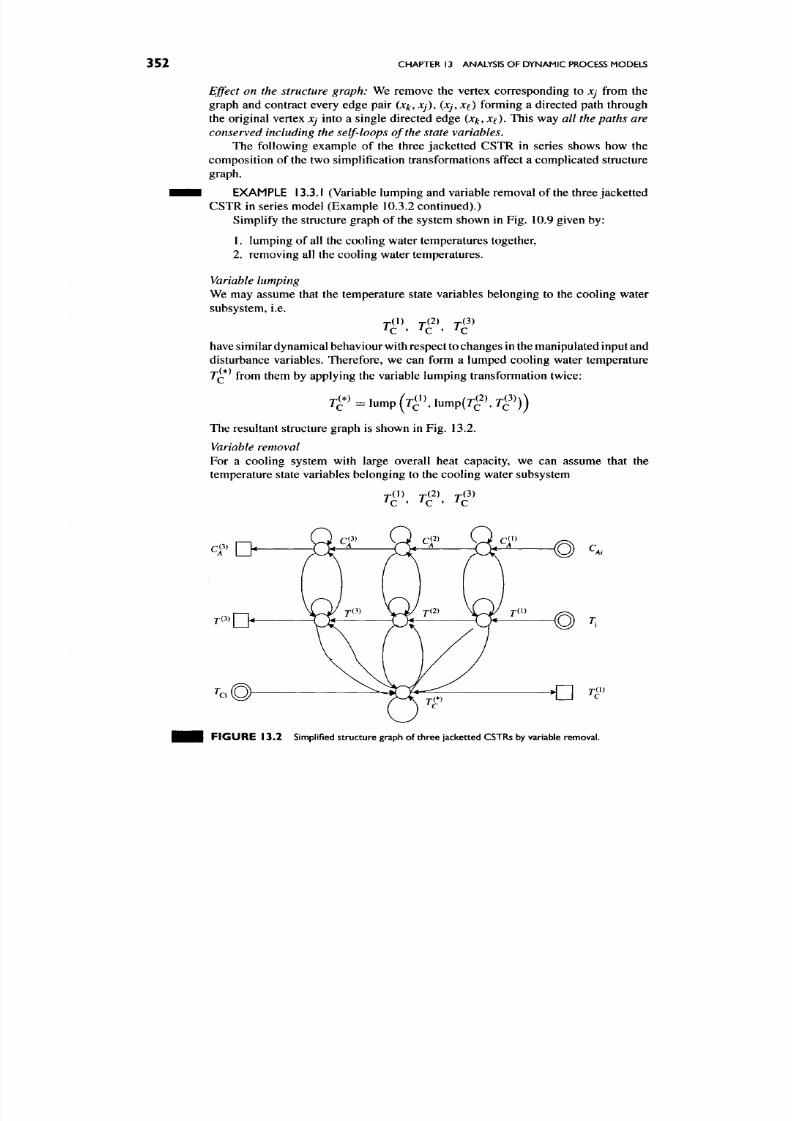
8/17/2019 Process Modelling and Model Analysis-Hangos-Cameron
http://slidepdf.com/reader/full/process-modelling-and-model-analysis-hangos-cameron 369/560
352
CHAPTER 13 ANALYSIS OF DYN AM IC PROCESS MODELS
Ejfect on the structure graph: We remove the vertex corresponding to Xj from the
graph and contract every edge pair {x^, Xj), (xj, x^) forming a directed path through
the original vertex Xj into a single directed edge
(x^,
x^). This way
all the paths are
conserved including the self-loops of the state variables.
The following example of the three jacketted CSTR in series shows how the
com position of the two simplification transformations affect a complicated structure
graph.
EXAMPLE 13.3.1 (Variable lumping and va riable removal of the three jack etted
CSTR in series model (Example 10.3.2 continued).)
Simplify the structure graph of the system show n in Fig. 10.9 given by:
1.
lumping of all the cooling water temperatures together,
2. removing all the cooling water temperatures .
Variable
lumping
We may assume that the temperature state variables belonging to the cooling water
subsystem, i.e.
^ ( 1 ) ^ ( 2 ) ^ ( 3 )
^C ' ^C ' ^C
have similar dynamical behaviour w ith respect
to
changes in the manipulated input and
disturbance variables. Therefore, we can form a lumped cooling water temperature
T^ from them by applying the variable lumping transformation twice:
r(*)
iump(r^^\iump(r^2\r^^>))
The resultant structure graph is shown in Fig. 13.2.
Variable removal
For a cooling system with large overall heat capacity, we can assume that the
temperature state variables belonging to the cooling water subsystem
nil)
x ( 2 )
r(3)
r^)
F I G U R E 13 ,2 Simplified structure graph of three jacketted CSTRs by variable removal.
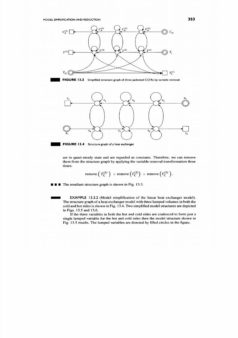
8/17/2019 Process Modelling and Model Analysis-Hangos-Cameron
http://slidepdf.com/reader/full/process-modelling-and-model-analysis-hangos-cameron 370/560
MODEL SIMPLIFICATION AND REDUCTION
353
FIGURE 13 .3 Simplified structure graph of three jacketted CSTRs by variable remova l.
FIGURE 13 .4 Structure graph of a heat exchanger.
are in quasi-steady state and are regarded as constants. Therefore, we can remove
them from the structure graph by applying the variable removal transformation three
times:
remove
( T^^ )
o remove
(T^^\
O remove
(T^^ )
.
The resultant structure graph is shown in Fig. 13.3.
EXAMPLE 13.3.2 (Model simplification of the linear heat exchanger m ode l).
The structure graph of a heat exchang er mod el with three lump ed volum es in both the
cold and hot sides is shown in Fig. 13.4. Two simplified mod el structures are depicted
in Figs. 13.5 and 13.6.
If the three variables in both the hot and cold sides are coalesced to form just a
single lumped variable for the hot and cold sides then the model structure shown in
Fig. 13.5 results. The lumped variables are denoted by filled circles in the figure.
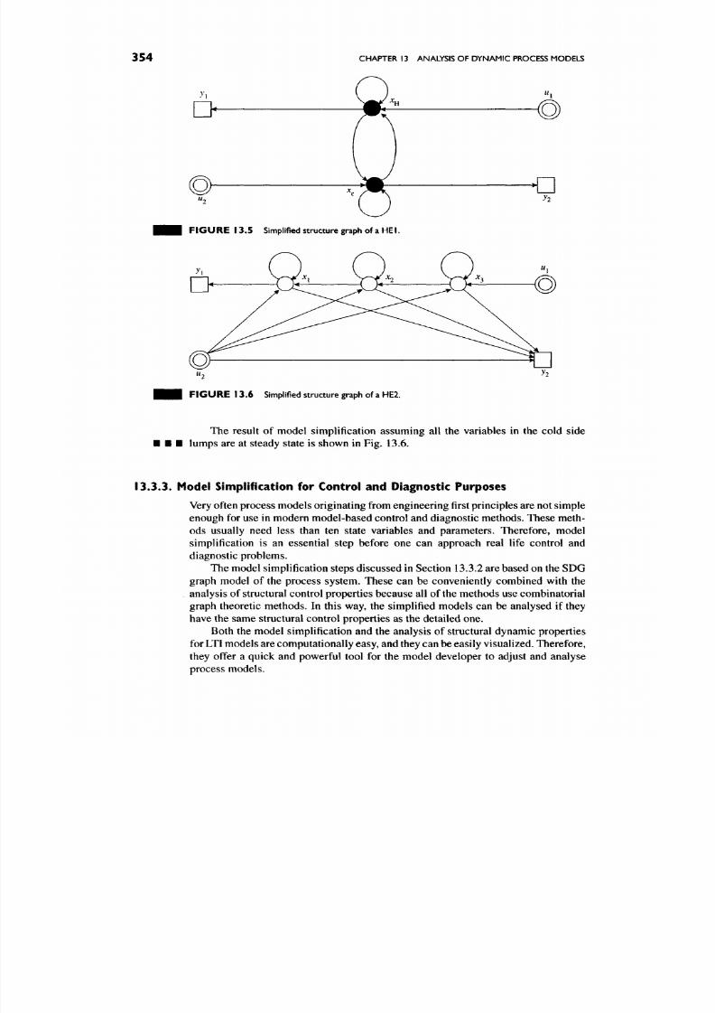
8/17/2019 Process Modelling and Model Analysis-Hangos-Cameron
http://slidepdf.com/reader/full/process-modelling-and-model-analysis-hangos-cameron 371/560
354
CHAPTER 13 ANALYSIS OF DYNAMIC PROCESS MODELS
yi
FIGURE 13 .5 Simplified struc ture graph of
a HE
I.
FIGURE 13 .6 Simplified structure graph of
a
HE2.
The result of model simplification assuming all the variables in the cold side
lumps are at steady state is shown in Fig. 13.6.
13.3.3.
Model Simplification for Control and Diagnostic Purposes
Very often process m odels originating from engineering first principles are not simple
enough for use in modern model-based control and diagnostic methods. These meth
ods usually need less than ten state variables and parameters. Therefore, model
simplification is an essential step before one can approach real life control and
diagnostic problems.
The model simplification steps discussed in Section 13.3.2 are based on the SDG
graph model of the process system. These can be conveniently combined with the
analysis of structural control properties becau se all of the methods u se com binatorial
graph theoretic methods. In this way, the simplified models can be analysed if they
have the same structural control properties as the detailed one.
Both the model simplification and the analysis of structural dynam ic prop erties
for
LTI
models are compu tationally easy, and they can be easily visualized. Therefore,
they offer a quick and powerful tool for the model developer to adjust and analyse
process models.

8/17/2019 Process Modelling and Model Analysis-Hangos-Cameron
http://slidepdf.com/reader/full/process-modelling-and-model-analysis-hangos-cameron 372/560
MODEL SIMPLIFICATION AND REDUCTION 3 5 5
The Effect of Model Simplification Transformations on Structural Properties
Both variable lumping and variable removal seriously affect the structure graph of
the system therefore it is important to know how these elementary transformations
influence the structural properties of the underlying system model.
1. Variable lumping
The lump ing transformation c onserves all the paths including self-loops and doe s
not lead to any direct paths from input to output vertices.
Therefore, the simplified structure graph:
• has self-loops adjacent to each of its state variable vertices, ensuring that the
state structure graph
[A]
has full structural
rank.
The state vertices again span
a strong com ponent in the structure graph;
• remains input connec tible. This property together with the fact that every input
variable is adjacent to a state variable from the strong component spanned by
the state variable vertices implies
structural controllability of the simplified
system in both the "Rich in inputs and outputs and the "Single input single
output'' cases;
• remains output connectible. Because of the same reasons as above the
simplified system is structurally observable in both of the cases.
2. Variable
removal
The variable removal transformation c onserves all the paths including self-loops
but may lead to direct paths from input to output vertices.
Therefore, the simplified structure graph:
• has self-loops adjacent to each of its state variable vertices, ensuring that
the
state structure graph [A] has ull structural
rank.
The state vertices again span
a strong component in the structure graph;
• rema ins input conn ectible for input variables which remain adjacent to a state
variable;
• remains output conn ectible for output variables which remain adjacent to a
state variable.
133.4. Model Reduction
As an alternative to model structure simplification there are analytical methods to
reduce the number of state variables of LTI state space models which have "similar"
input-output behaviour. This alternative way is called
analytical model reduction.
Model reduction is done in two conceptual steps:
1. construction of the so-called
balanced realization
using similarity trans
formations and the compu tation of controllability and observability gram ians;
2. reducing the balanced state space realization by omitting those trans
formed states which do not contribute significantly to the observability and
controllability gramians of the system.
It is clear from the above conce ptual description that the reduced order model
does not only c ontain fewer state variables but its state variables are transformed
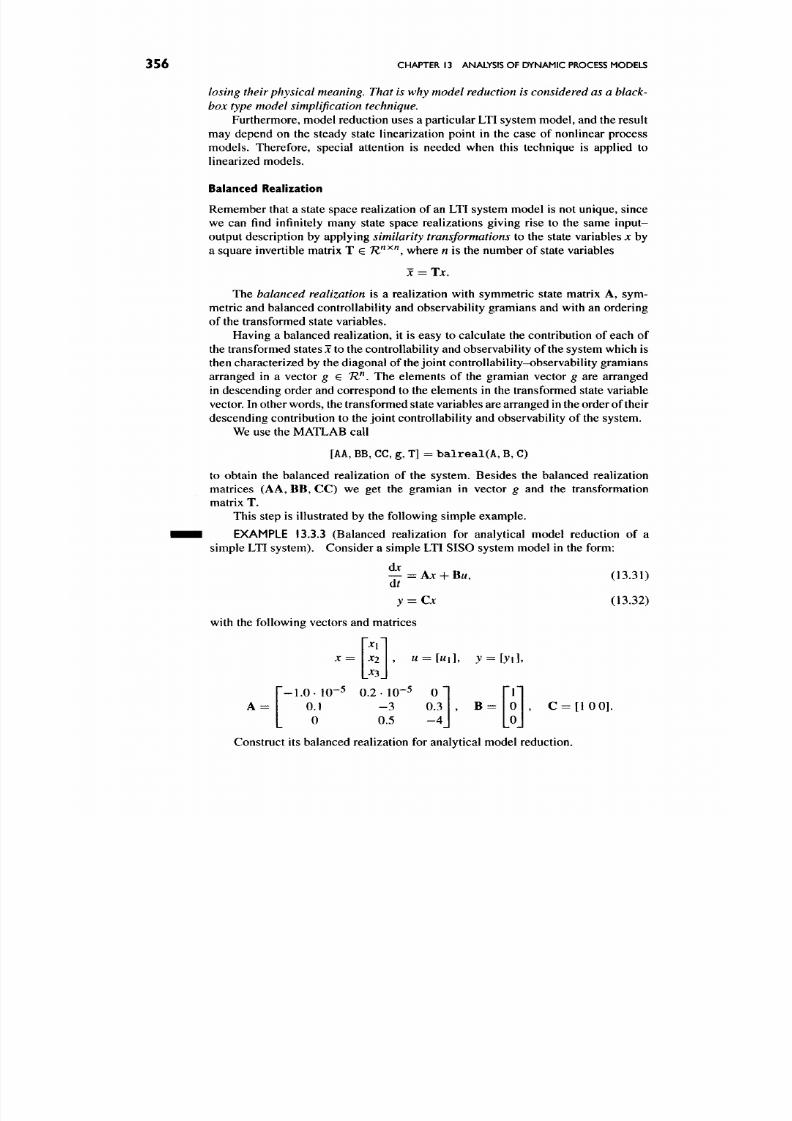
8/17/2019 Process Modelling and Model Analysis-Hangos-Cameron
http://slidepdf.com/reader/full/process-modelling-and-model-analysis-hangos-cameron 373/560
356
CHAPTER 13 ANALYSIS OF DYN AM IC PROCESS MODELS
losing their physical
meaning.
That is why m odel reduction is considered as a
black-
box type m odel simplification technique.
Furtherm ore, model reduc tion uses a particular LTI system mod el, and the result
may depend on the steady state linearization point in the case of nonlinear process
models. Therefore, special attention is needed when this technique is applied to
linearized models.
Balanced Realization
Remember that a state space realization of an LTI system model is not unique, since
we can find infinitely many state space realizations giving rise to the same input-
output description by applying similarity transformations to the state variables x by
a square invertible matrix T
e K^^^,
where
n
is the number of state v ariables
X
= Tx.
The balanced realization is a realization with symmetric state matrix A, sym
metric and balanced controllability and observability gramians and with an ordering
of the transformed state variables.
Having a balanced realization, it is easy to calculate the contribution of each of
the transformed states x to the controllability and ob servability of the system w hich is
then characterized by the diagonal of
the
joint controllability-observability gramians
arranged in a vector
g e
TV^. The elements of the gramian vector
g
are arranged
in descending order and correspond to the elements in the transformed state variable
vector. In other words, the transformed state variables are arranged in the order of their
descending contribution to the joint controllability and observability of the system.
We use the MATLAB call
[AA,
BB, CC, g , T] = ba l re a l (A ,
B,
C)
to obtain the balanced realization of the system. Besides the balanced realization
matrices (AA, BB , CC ) we get the gramian in vector
g
and the transformation
matrix T.
This step is illustrated by the following simple exam ple.
EXAMPLE 13.3.3 (Balanced realization for analytical model reduction of a
simple LTI system). Consider a simple LTI SISO system model in the form:
djc , _
— =
AJC + BM,
At
y = Cx
with the following vectors and matrices
(13.31)
(13.32)
X —
- 1 . 0 - 1 0 - ^
0.1
0
Xi
X2
0.2 . 10-^
- 3
0.5
w = [wi], y = \y\\.
o '
0.3
- 4
, B =
' l 1
0
0
C = : [ 1 0 0 ] .
Construct its balanced realization for analytical model reduction.
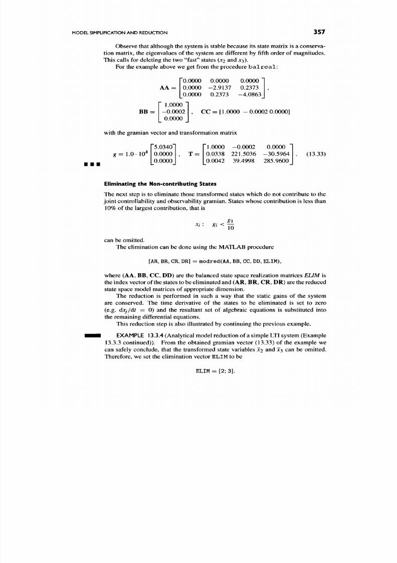
8/17/2019 Process Modelling and Model Analysis-Hangos-Cameron
http://slidepdf.com/reader/full/process-modelling-and-model-analysis-hangos-cameron 374/560
MODEL SIMPLIFICATION AND REDUCTION
357
Observe that although the system is stable because its state matrix is a conserva
tion matrix, the eigenvalues of the system are different by fifth order of m agnitud es.
This calls for deleting the two "fast" states (x2 and JC3).
For the example above we get from the procedure b a l r e a l :
BB =
AA =
0.0000 0.0000 0.0000
0.0000 -2. 91 37 0.2373
0.0000 0.2373 -4.0863
1.0000
- 0 .0 0 0 2
0.0000
, CC = [ 1.0000 - 0.0002 0.0000]
with the gramian vector and transformation matrix
g= 1.0 lO
5.0340
0.0000
0.0000
T
=
1.0000 -0.0002 0.0000
0.0338
221.5036 -30.5964
0.0042 39.4998 285.9600
(13.33)
Eliminating the Non-contributing States
The next step is to eliminate those transformed states which do not contribute to the
join t controllability and observability g ramian . States whose contribution is less than
10% of the largest contribution, that is
gi <
8±
10
can be omitted.
The elimination can be done using the MATLAB procedure
[AR, BR, OR, DR] = modred(AA, BB, CC, DD, ELIM),
where (AA, BB , CC , DD) are the balanced state space realization matrices
ELIM
is
the index vector of the states to be eliminated and (A R, BR , CR , D R) are the reduced
state space model matrices of appropriate dimension.
The reduction is performed in such a way that the static gains of the system
are conserved. The time derivative of the states to be eliminated is set to zero
(e.g.
dxj/dt =
0) and the resultant set of algebraic equations is substituted into
the remaining differential equations.
This reduction step is also illustrated by continuing the previous example.
EXAMPLE 13.3.4 (Analytical model reduction of a simple LTI system (Exam ple
13.3.3 continu ed)). From the obtained gramian vector (13.33) of the example we
can safely conclude, that the transformed state variables X2 and JC3 can be omitted.
Therefore, we set the elimination vector ELIM to be
ELIM = [2; 3] .
8/17/2019 Process Modelling and Model Analysis-Hangos-Cameron
http://slidepdf.com/reader/full/process-modelling-and-model-analysis-hangos-cameron 375/560
358 CHAPTER 13 ANALYSIS OF DYNAM IC PROCESS MODELS
Using the MATLAB procedure m o d re d for the reduction we obtain the following
reduced SSR:
AR = [-9.9325 • 10"^ ], BR = [1.0000], CR = [1.0000],
• • • DR = [-7.8905 • 10"^]. (13.34)
13.3.5. Relation between Model Reduction and
Model Structure Simplification
It is easy to see from the above and from the description of the model structure sim pli
fication steps that
m odel reduction is the analytical version of a sequence of variable
removal structure simplification steps
if one does not apply the transformation to get
a balanced realization.
In order to show this, consider the reduction principle and formulate this in
mathematical terms. First we partition the state variable vector x into x i to be kept
and
X2
to be eliminated and partition all the SSR matrices accordingly:
|]=[A;;i;3][s]4y«-
y = [Ci
C2]JC
+ DM. (13.36)
Next we set the derivative of
JC2
to zero and the resulting algebraic equation is solved
for X2 and substituted into the remaining ones to get:
^ = [ A U -Ai2A^2^A2i] jc , + [ B I - A I 2 A - 2 ^ B 2 ] M , (13.37)
J = Tci - C2A~2^A2il Jci + [ D - C2A~2^B2] u. (13.38)
Note that the MATLAB procedure m o d r e d can be used to compute the weights
of the reduced structure graph m odel after v ariable removal simplification steps.
EXAMPLE 13.3.5 Analytical model reduc tion and model structure simplifica
tion by variable removal of a simple LTI system (Exam ple 13.3.4 continued ).
If we want to compute the state space model parameters after simplification by
variable removal we set the elimination vector EL IM to be
ELIM = [2; 3]
to eliminate states X2 and x^ bu t now from the original state space realization.
Using the MATLAB procedure modred for the reduction again we obtain the
following reduced SSR:
AQ =
[-9.9325
• 10"^], BQ = [1], CQ = [1], DQ = [0]. (13.39)

8/17/2019 Process Modelling and Model Analysis-Hangos-Cameron
http://slidepdf.com/reader/full/process-modelling-and-model-analysis-hangos-cameron 376/560
FURTHER READING
359
Comparing this reduced model with the original one in Eq. (13.34) using balanced
realization we see that there is almost no difference in this case. However, the results
are structurally different because in the simplified structure, we do not have a direct
influence from the input to the output. In the reduced case, however, we have one but
• • • its mag nitude is negligible com pared to the other influences.
13.4. SUMMARY
In this chapter, we have investigated some key concepts applicable to models specif
ically developed for process control applications. In particular the concepts of
observability and controllability are extremely im portant for control application s. The
idea of stability was introduced and investigated in relation to linear time-invariant
models. These constitute a very large class of problems in control applications and
are amenable to analysis through well established techniques.
The second part of the chapter has been devoted to the analysis of structural
dynamical properties which hold for a class of systems with the same structure.
The concepts and analysis techniques of structural controllability, observability and
stability are based on graph theory.
Finally, analytical and structural methods for mo del simplification and reduction
have also been presented and compared.
13.5.
FURTHER READING
The analysis of dynamic process models in itself is rarely the subject of any book,
papers, conference or other information source, but it appears as an integral part of
process design or process control studies. Therefore, there is a big overlap between
the information sources of dynamic analysis and control or design of process systems.
The most important sources are as follows.
• Journals
- Journal of Process Control
- Industrial and Engineering Chemistry Research
- Com puters and Chemical Engineering
- AICh E Journal
•
Conferences
- AIChE Meetings
- ESC APE Conferences
- IFAC Conferences "ADCHEM " and "DYC ORD "
- IFAC World Congresses
- PSE Conferences
• Web Control Engineering Virtual Library, with homepage:
http://www-control.eng.cam.ac.uk/extras/Virtual_Library/
Control^VL.html.
There are a few "hot topics" in connection with the analysis of dynamic process
modelling which deserve special attention.
8/17/2019 Process Modelling and Model Analysis-Hangos-Cameron
http://slidepdf.com/reader/full/process-modelling-and-model-analysis-hangos-cameron 377/560
360 CHAPTER 13 ANALYSIS OF DYN AMI C PROCESS MODELS
• Interaction between process design and control
The interaction between process design and control had been recognized a
long time ago and the use of open-loop dynam ic indicators has been sugg ested
for assessing the controllability and o perability of design alternatives [89 ].
There are advanced spectral methods for
the
analysis and design of process
dynamics which are reviewed and applied in a recent PhD Thesis [90].
There are several recent research papers which perform integration of
design and control through model analysis, such as [91].
• Operability analysis of process plants
Operability is the property of a process plant characterizing its behaviour
under changing operating conditions. Design alternatives are assessed with
respect to their operability using structural and simple linearized operability
measures [92].
A simulation-based methodology has been reported in [93] for evaluating
the stability of control structures and finding the best flowsheet structure from
a controllability point of view.
• Mode l simplification and reduction
Various techniques for m odel simplification and reduction have been proposed
ranging from the simplest linear techniques to very complex nonlinear ones.
A wavelet-based model reduction method has been proposed in [94] for
distributed parameter systems.
13.6. REVIEW QUESTIONS
Q13.1. Give the problem statement of state controllability and observability.
(Section 13.1).
Q13.2.
Com pare the notions of BIBO and asymptotic stability. Which one is the
stronger? Give a process exam ple which is BIBO stable but not asymptotically stab le
(Section 13.1)
Q13.3.
Wh at is the relation between a dynam ical property (say stability) and its
structural counterpart (structural stability). Does the structural dynamical property
imply that property for
every
dynamical system in the class? (Section 13.2)
Q13.4.
Wh at is the physical condition which causes the state structure matrix of
a process system to almost always be of full structural rank? Give simple process
examples. (Section 13.2)
Q13.5. Give conditions which ensure the structural controllability of a system
mod el. In which case are they equivalent? (Section 13.2)
Q13.6. Give conditions which ensure the structural observability of a system model.
In which case are they equivalent? (Section 13.2)
Q13.7. When do we call a matrix a conservation matrix? Are conservation matrices
of full structural rank? Why? (Section 13.2)
Q13.8. Give the problem statement of model simplification. Derive its special case
for linear state space mod els. (Section 13.3)
8/17/2019 Process Modelling and Model Analysis-Hangos-Cameron
http://slidepdf.com/reader/full/process-modelling-and-model-analysis-hangos-cameron 378/560
APPLICATION EXERCISES 361
Q13.9. W hat are the two model simplification op erations one applies for simpli
fication of linear process models? Do they change the structural controllability and
observability properties of the model? (Section 13.3)
Q13.10. Com pare the analytical model reduction with mod el structure sim plification.
What are the similarities and the differences? Is it possible to use a combination of
the two? How? (Section 13.3)
13
J .
APPLICATION EXERCISES
A13.1. Com pute the observability matrices of the LTI systems given in Exam ples
10.2.2 and 10.2.3 and check if the systems are observable. (Section 13.1)
A13.2. Com pute the controllability matrices of the LTI systems given in Exam ples
10.2.2 and 13.1.3 and check if the systems are controllable. (Section 13.1)
A13.3. Derive the signed structure matrix form of the linearized state space model
matrices of the batch water heater in Example 14.3.1 derived from its SDG model
shown in Fig. 14.2. Com pare them with that derived from the lumped m odel equations
(14.36) and (14.37). (Section 13.2)
A
13.4.
Derive the signed structure graph model of the LTI state space model m atrices
in Example 10.2.1. Is this model structurally controllable and observable? Com
pare your findings with the analytical results given in Examples 13.1.2 and 13.1.5.
Comment on the similarities and possible differences. (Section 13.2)
A13.5. Check if the state space matrices of the LTI system mo dels of the Exam ples
10.2.1 and 10.2.3 are conservation matrices. Are the corresponding model struc
tures structurally stable? Compare your findings with the analytical results given in
Examples 13.1.7 and 13.1.8. Comment on the similarities and possible differences.
(Section 13.2)
A13.6. Is the state space model of the batch water heater (Eqs. (14.36) and (14.37))
structurally observable and controllable? Check it by graph theoretic methods on
its SDG model shown in Fig. 14.2. Compare the result with the one obtained by
computing the rank of the observability and controllability matrices {O and C of the
same model giving numerical value to the model parameters). (Section 13.2)
A13.7. Is the state space model of the batch water heater (Eqs. (14.36) and (14.3 7))
structurally stable? Check it by the method of conservation m atrices using the signed
structure matrix derived in Exercise A13.3. Compare the result with the one obtained
by com puting the eigenvalues of the state matrix A of the same mod el giving numerical
value to the model parameters. (Section 13.2)
A 13.8. A linear time invariant (LTI) system m odel leads to the following state space
model equ ations:
~At
•-2.0 1.3
1.2 - 4 . 0 1.2 I x l - I 0 I 'M ,
0 0
0
1.2
-3 .0
•JC +
'1.41
0
0 J
y = [4.2 0 0 ] j c .

8/17/2019 Process Modelling and Model Analysis-Hangos-Cameron
http://slidepdf.com/reader/full/process-modelling-and-model-analysis-hangos-cameron 379/560

8/17/2019 Process Modelling and Model Analysis-Hangos-Cameron
http://slidepdf.com/reader/full/process-modelling-and-model-analysis-hangos-cameron 380/560
PROCESS MODELLING
FOR
CONTROL AND DIAGNOSTIC
PURPOSES
Process control and diagnosis is the application area where dynamic process models
are extensively used. This chapter contains the necessary material for a process en
gineer
to understand and successfully use modern model-based process control and
diagnostic methods. The presentation of the material is therefore much more appli
cation oriented than the case would be in a book designed for control engineers. The
methods and procedures are described in terms of
Problem statements
and detailed
derivation of the metho ds or procedu res are usually left ou t. The conditions of app lic
ability of the particular methods and the evaluation of the results from a process
engineering perspective are emphasized.
Dynamic process models for control and diagnostic purposes are almost always
lumped process models in the form of DAE systems with given initial conditions.
Therefore, only lumped dynamic process models are considered throughout this
chapter.
In Section 14.1 the modelling requirem ents for process control are form ulated
and analysed together with the problem statements and conceptual solution of
the most frequently used state space model-based control problems.
The process models suitable for diagnosis and the most important approaches
for process diagnosis are discussed in Section 14.2.
Finally a brief survey of qualitative, logical and artificial intelligence pro
cess models and their use for control and diagnostic purposes is given in
Section 14.3.
363
8/17/2019 Process Modelling and Model Analysis-Hangos-Cameron
http://slidepdf.com/reader/full/process-modelling-and-model-analysis-hangos-cameron 381/560
364 CHAPTER 14 PROCESS MODELLING FOR CON TRO L AN D DIA GNOST IC PURPOSES
14.1.
MODEL-BASED PROCESS CONTROL
Until now we have mainly dealt with
systems analysis,
when process systems
have been investigated as they are, without any intention to influence their nat
ural behaviour.
Control theory deals with the problems, concepts and techniques
to influence the behaviour of systems to achieve some prescribed goal.
Besides control in the above narrow sen se, all the other subtasks w hich are either
related to control or involve some decision concerning dynamic systems belong to
the area of control theory, such as
• identification (model parameter and structure estimation),
• filtering, state filtering, prediction and smo othing,
• diagnosis (fault detection and isolation).
In this section, we briefly review the most imp ortant control related tasks relevant
to process engineering.
14.1.1.
Feedback
Feedback is a central notion in control theory. Most of the con trollers, but not all of
them, apply either state or output feedback to compute the control ac tion.
It is intuitively clear that one should take into account the effect of the previously
applied input values when computing the present one through the dependence of the
input value on the observed outputs or the states - that is to apply feedback.
If the present control action, that is the applied input d epends on the value of the
state variables, then a state feedback is applied for control
u = F{x),
(14.1)
where F is a known, possibly nonlinear function.
Output feedback is defined similarly but then
u = Fiy). (14.2)
Feedback s can be classified according to the function
F
in the feedback equation
as follows:
1.
static feedback
— whe n F is a time invariant algebraic operator,
2. full feedback— when F d epends on every element in the state or output vector
respectively,
3. linear feedback—when F is a linear operator.
For LTI systems most of the controllers apply
linear static full state feedback
in
the following form:
M
=
KJC,
(14.3)
where the constant matrix K with appropriate dimension is the
control gain.
8/17/2019 Process Modelling and Model Analysis-Hangos-Cameron
http://slidepdf.com/reader/full/process-modelling-and-model-analysis-hangos-cameron 382/560

8/17/2019 Process Modelling and Model Analysis-Hangos-Cameron
http://slidepdf.com/reader/full/process-modelling-and-model-analysis-hangos-cameron 383/560
3 6 6 CHAPTER 14 PROCESS MODELLING FOR CON TRO L
A N D
DIA GNO STIC PURPOSES
3. The
controller
design method does not
require
the solution of the model equa
tions but only uses the model parameter values.
It means that as soon as the
controller parameters are computed the controller does not perform heavy
computations in real time.
4.
The software package MATLAB has a simple procedure (place) to compute
the feedback gain vector from the SSR m atrices of the open-loop system and
from the desired poles.
• • • EXAMPLE 14.1.1 (Pole-placement controller design for a simple LTI system).
Consider a simple SISO LTI system in the form of E q. (14.4) with the matrices
4 ^
B =
C = [1 0] . (14.9)
Let the desired po les of the closed-loop system be —1 and — 3. Then the pole-
placement controller design procedure chec ks the full rank of the con trollability matrix
and gives the following feedback gain vector:
it = [0.5455 1.2727]. (14.10)
14.1.3. Linear Quadratic Regulator (LQR)
Linear quadratic regulators (LQRs) are widely used in process control. Its popularity
is explained by the fact that it is quite robust with respect to modelling uncertainties.
Generalised versions are also available for classes of linear time-varying, special
nonlinear and robust linear models.
The problem statement and the solution of the LQR design problem is as follows:
LINEAR QUADRATIC REGULATOR DESIGN
Given:
• A continuous time LTI state space model of a M IMO system in the form:
^ = A J C +
BM,
JC(0)=JCO, (14.11)
d^
y = Cx (14.12)
with its matrices (A, B, C)
• A loss functional J{x, u)
1
C^
J(x,
M) = - /
[x^iOQxit)
+
u'^{t)Ru{t)]
dr (14.13)
2 Jo
with a positive semidefinite state weighting matrix Q and with a positive def
inite input weighting matrix R where identically zero state reference value
^(ref) _ 0 is assum ed. (See Section A .4.1 in the appendix for the definition of
positive definite and semidefinite matrices.)

8/17/2019 Process Modelling and Model Analysis-Hangos-Cameron
http://slidepdf.com/reader/full/process-modelling-and-model-analysis-hangos-cameron 384/560
MODEL-BASED PROCESS CONTROL 367
Compute:
A control signal
[u{t)\Q<t< T), (14.14)
that minimizes the loss function (14.13) subject to model equations (14.11).
Solution [70]:
For
the stationary case, when
7 -> oo,
the solution is a full state feedback controller
which stabilizes the system and at the same time gives the minimal loss provided the
system is jointly controllable and observable.
The solution of the mathematical problem in the stationary case leads to the solu
tion of the so-called control algebraic Ricatti equation (CARE), which is a quadratic
equation for a square matrix. In this case this equation has a unique solution from
which the full state feedback matrix can be easily computed.
The software package MATLAB has a simple procedure (Iqr) to compute the
feedback gain matrix from the state-space representation matrices of the open-loop
system and from the weighting matrices in the loss functional.
• • • EXAMPLE 14.1.2 (LQR design for a simple LTI system introduced in Exam ple
14.1.1). Con sider a simple SISO LTI system in the form of Eq. (14.4) with the
matrices in Eq. (14.9).
Let the weighting matrices in the loss function (14.13) be as follows:
Q = [ o i ] , R = [0 .5 ] . (14.15)
This me ans that we w eight the error in the state or output much higher than the effort
in changing the input.
Then the LQR design procedure in MATLAB gives the following feedback gain
matrix which is now a row vector because we have a SISO system:
it = [0.9898 0.8803 ]. (14.16)
The poles of the closed-loop system
[-15.2021 -8 .7690]
• • • indeed have negative real parts which means that the closed-loo p system is stable.
14.1A State Filtering
Both of the above controller design methods apply full state feedback to realize the
controller. Therefore one should be able to compute the non-m easurable state variables
from the measured input and output variables using only the system model. In the
case of an observable deterministic LTI system, there is a direct way how to do this
making use of the observability matrix O.
However,
in the presence of any random elem ents in the model, either measure
ment
errors
or system noise, w e have to estimate the value of the state variables from
the measured input and output variables using the system m odel. This procedure is

8/17/2019 Process Modelling and Model Analysis-Hangos-Cameron
http://slidepdf.com/reader/full/process-modelling-and-model-analysis-hangos-cameron 385/560
3 68
CHAPTER 14 PROCESS MODEL LING FOR CO NT RO L A N D DIAG NOS TIC PURPOSES
called state filtering.
Th e problem statement and the conceptual steps of the solution
are described below.
STATE
FILTERING
Given:
• A
discrete time stochastic LTI state space m odel
represented by
jc(r + 1) = ^ JC (T ) +
TU(T)
+ v(r ), jc(0) =
XQ,
(14.17)
y{T) = C jc(r)
-f
e ( r ) ,
r = 0,
1, 2 , . . . (14.18)
with
its
model matrices (^ ,
T, C)
and
with
the properties of an additive system
and measureme nt noise v(r ) a nd e{x) being independent random variables at
anytime x.
• A measurement record being a set of data corrupted by measurement noise
V{h k]
=
{(M(T), y{T)) I
r =
1 ,. . . , M. (14.19)
Compute:
An estimate of the current state vector jc(/:) based on the measurement record V[l,k]
and the system parameters.
Solution [74]:
For the LTI case when both the state noise and measurement noise processes are
Gaussian white noise processes, the famous Kalman-filter can be used to solve the
problem.
The K alman filter u ses a simple linear filter equation to be computed in real
time:
X(T -f 1) = ^ JC (T ) + rM(r) + K(T)Cv(r) - CJC(T) ) ,
JC(0)
=
JCQ,
(14.20)
where X(T) is the state estimate in time T and K(r) is the Kalman gain. Note that
this filter equation
is
very similar to the state equation (14.17) but the state noise
is
replaced by its estimate based on the output equation (14.18).
The sequence
of
Kalman gains K ( T ) ,
T = 0,
1 , . . . can be precomputed using
the model parameters
in a
recursive way. This sequence is then used to compute the
estimate using the filter equation (14 .20).
The software package MATLAB
has
procedures
to
compute
the
sequence
of
Kalman gains as well as the sequence of the state estimate (Kalman).
14.1.5. Model-based Predictive Control
Model-based predictive control (MPC) is the most popular and widely used method
for advanced process control. Its popularity is partially explained by the availability of
reasonable good and reliable process models and implementations on commercially
available control systems.
Mo reover the basic idea behind m odel-based predictive control is simple, easy to
understand and yet powerful. If one has a dynam ic process mo del which is reasonably
accurate and validated then this model can be used for predicting how the real process
system would behave by applying a specific control signal, either discrete or contin
uous
to its
input. This predicted output behaviour
is
then compared
to
the desired

8/17/2019 Process Modelling and Model Analysis-Hangos-Cameron
http://slidepdf.com/reader/full/process-modelling-and-model-analysis-hangos-cameron 386/560
MODEL-BASED PROCESS CONTROL 369
or reference output using a suitably chosen distance between signals (measured by a
signal norm). If the predicted behaviour is not "close enough" to the desired one then
another control signal is tested. Otherwise, the control signal is applied to the real
process system.
The problem statement of model-based predictive control and the conceptual
steps of the solution are described below.
MODEL-BASED PREDICTIVE CONTROL
Given:
• A parametrized sam pled predictive dynamic system model in the form of
y(^)(k + 1) = M(V[\,k]:
/7^^>),
ik = 1, 2 , . . . (14.21)
with the model parameters p^^^ e K^ being known, a measured data record
T>[\,k]eU^
up to time
k
and a vector-valued output variable
y^^\k)
e IV^.
• A set of measured data which is called a measurement record to emphasize
the time dependence of the measured data
V[\,k] = {(M(r),y{T)) I r = 1 , . . . , ^} . (14.22)
• A reference output signal
{/'•)(/:) I /: = 1 , 2 , . . . } . (14.23)
• A prediction horizon N
• A
loss functional J^^^
N
j(^)(y(^)-y('), u)
= J2
[^^(^+OQK^+0-f-w'^(^+ORw(A:+0], (14.24)
/=
where r is the residual
r(k) =
y^'\k)
-
y^^\k). A: = 1, 2 , . . . (14.25)
with a positive semidefinite output weighting matrix Q and with a positive
definite input weighting matrix R.
Compute:
A discrete time control signal
[uik + i)\i= 1,...,A^ }, (14.26)
that minimizes the loss function (14.24) subject to the model equations (14.21).
Conceptual solution
method:
In the general case we can solve the problem as an optimization problem minimizing
the functional (14.24) as a function of the discrete time control signal (14.26). This
breaks down the problem into an optimization and a simulation step in a similar way
as for the parameter estimation of dynamic nonlinear models in Section 12.4.3.
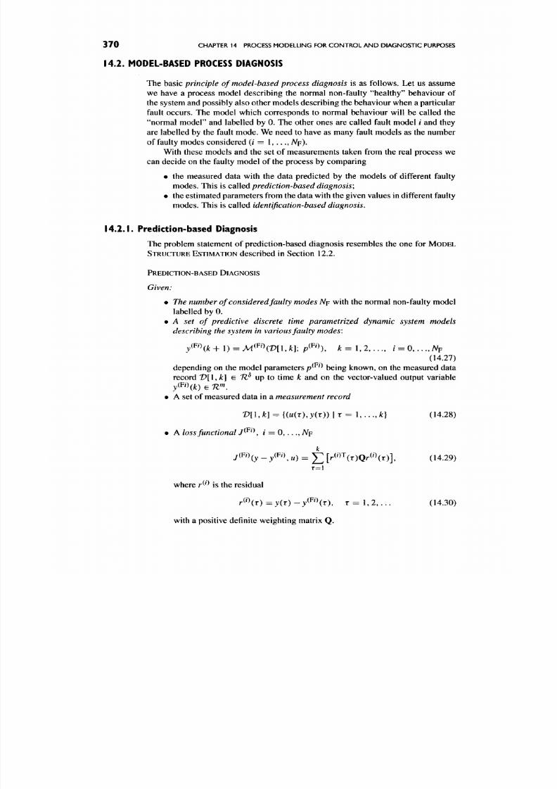
8/17/2019 Process Modelling and Model Analysis-Hangos-Cameron
http://slidepdf.com/reader/full/process-modelling-and-model-analysis-hangos-cameron 387/560

8/17/2019 Process Modelling and Model Analysis-Hangos-Cameron
http://slidepdf.com/reader/full/process-modelling-and-model-analysis-hangos-cameron 388/560
MODEL-BASED PROCESS DIAGNOSIS 37 I
Compute:
The faulty mode of the system, which is the model index / that minimizes the loss
function (14.29) subject to model equations (14.27).
Conceptual solution
method:
The solution is computed in two steps.
1. Perform the prediction with each of the models
M^^^\
/ = 0 , . . . ,
Nfj
and
compute the loss (14.29).
2. Select the mod el index with the minimum lo ss.
14.2.2.
Identification-based Diagnosis
Identification-based diagnosis uses the estimated set of model parameters in each
of the fault models and then compares them to their "true" values as seen from the
problem statement below.
IDENTIFICATION-BASED DIAGNOSIS
Given:
•
The number of considered faulty modes
A p with the normal non-faulty model
labelled by 0.
•
A set of parametrized discrete time dynamic system m odels describing the
system in various faulty modes:
y^^i\k
+ 1) =
M^^'\V[\,
k] \
p^^'^),
^ = 1 , 2 , . . . , / = 0 , . . . ,
TVp
(14.31)
depending on the m odel parameters
p^^^^
being known, on the measured data
record V[\,k\
e IZ^
up to time
k
and on the vector-valued output variable
y^^'\k) e W,
• A set of measured data in a
measurem ent record
D [ l ,
k] =
{(M(r),
y(T)
I r = 1 , . . . , ^} . (14.32)
• A
loss functional J^^'\
/ = 0 , . . . ,
A F
depending now on the parameters
y(FO(^(estFO _ ^(FO) ^
piOTQ^U)
(14 33)
where p^^^ is the parameter residual
p (0^^ (es tFO _^(FO (14 34)
with a positive definite weighting matrix Q and p ^ ^ ^ ^ ^ ^ ^ is the estimated
parameter vector of the model with faulty mode /.
Compute:
The faulty m ode of the system, which is identified by the model index / that minimizes
the loss function (14.33) subject to the model equations (14.31).
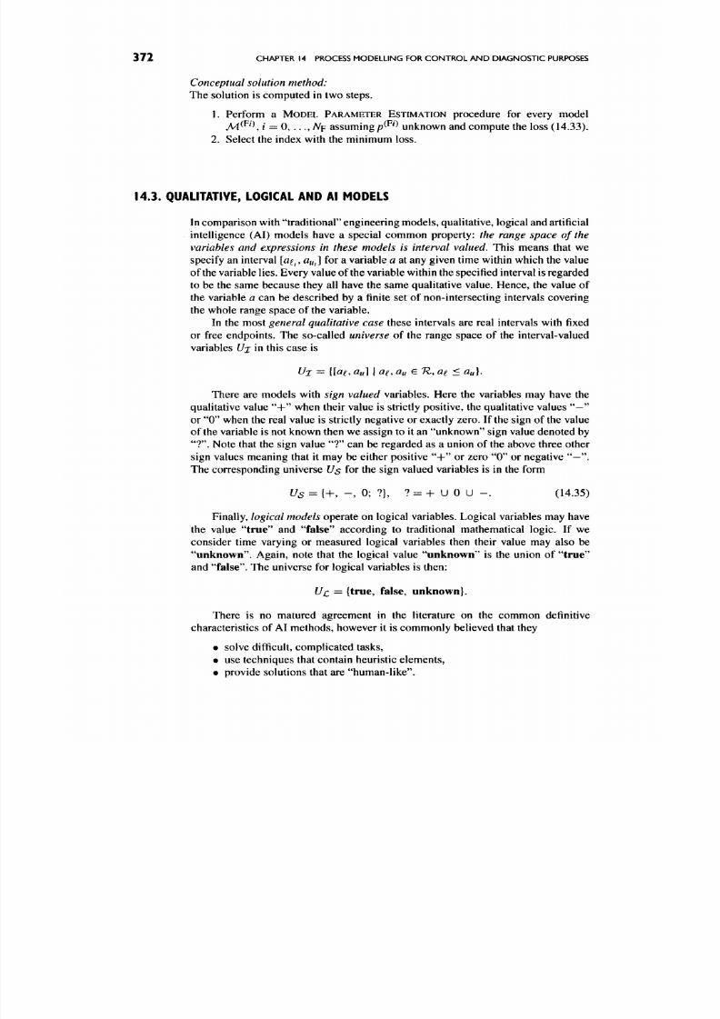
8/17/2019 Process Modelling and Model Analysis-Hangos-Cameron
http://slidepdf.com/reader/full/process-modelling-and-model-analysis-hangos-cameron 389/560
372
CHAPTER
14
PROCESS MODELLING FOR CO NTR OL AN D DIAG NOST IC PURPOSES
Conceptual solution
method:
The solution is computed in two steps.
1. Perform a MODEL PARAMETER ESTIMATION procedure for every model
assuming
p^^^^
unknown and compute the loss (14.33).
2. Select the index with the minimum loss.
14.3.
QUALITATIVE, LOGICAL AND Al MODELS
In comparison with "traditiona l" engineering mo dels, qualitative, logical and artificial
intelligence (AI) models have a special common property: the range space of the
variables and expressions in these models is interval
valued. This means that we
specify an interval
[a^^,
a„J for a variable
a
at any given time within which the value
of the variable
lies.
Every value of the variable within the specified interval is regarded
to be the same because they all have the same qualitative value. Hence, the value of
the variable a can be described by a finite set of non-intersecting intervals covering
the whole range space of the variable.
In the most general qualitative case these intervals are real intervals with fixed
or free endpoints. The so-called
universe
of the range space of the interval-valued
variables Uj in this case is
Uj =
[[ae, au]
\ a ^
au
e
7^,
a^ < au].
There are models with
sign valued
variables. Here the variables may have the
qualitative value
"-I-"
when their value is strictly positive, the qualitative values "—"
or " 0 " when the real value is strictly negative or exactly zero. If the sign of the value
of the variable is not known then w e assign to it an "unkn own " sign value denoted by
"?". Note that the sign value " ? " can be regarded as a union of the above three other
sign values meaning that it may be either positive "-I-" or zero "0" or negative "—".
The corresponding universe Us for the sign valued variables is in the form
Us = {+ , - , 0 ; ?},
?
= + U 0 U - . (14.35)
Finally,
logical models
operate on logical variables. Logical variables may have
the value "true" and "false" according to traditional mathematical logic. If we
consider time varying or measured logical variables then their value may also be
"unknown". Again, note that the logical value "unknown" is the union of "true"
and "false". The universe for logical variables is then:
Uc
= {true, false, unknown}.
There is no matured agreement in the literature on the common definitive
characteristics of AI methods, however it is commonly believed that they
• solve difficult, complicated tasks,
• use techniques that contain heuristic elemen ts,
• provide solutions that are "hum an-like".
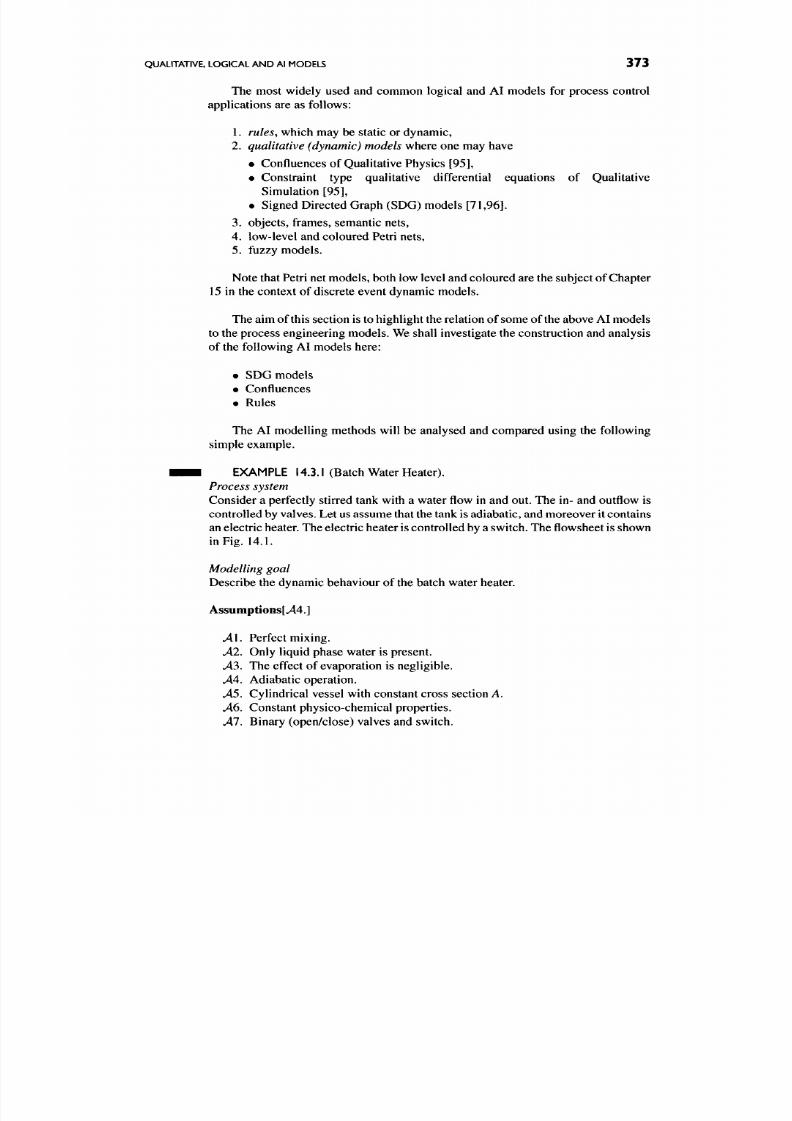
8/17/2019 Process Modelling and Model Analysis-Hangos-Cameron
http://slidepdf.com/reader/full/process-modelling-and-model-analysis-hangos-cameron 390/560
QUALITATIVE. LOGICAL AND Al MODELS
373
The most widely used and common logical and AI models for process control
applications are as follows:
1.
rules, which may be static or dynamic,
2.
qualitative (dynamic) models
w here one may have
• Confluences of Qualitative Physics [95],
• Con straint type qu alitative differential equations of Q ualitative
Simulation [95],
• Signed Directed Graph (SDG) models [71,96].
3.
objects, frames, semantic nets,
4.
low-level and coloured Petri nets,
5. fuzzy models.
Note that Petri net mod els, both low level and coloured are the subject of Chap ter
15 in the context of discrete event dynamic models.
The aim of this section is to highlight the relation of some of the above A I mod els
to the process engineering mo dels. We shall investigate the construction and analysis
of the following AI models here:
• SDG models
• Confluences
• Rules
The AI modelling methods will be analysed and compared using the following
simple example.
• • • EXAMPLE 14.3.1 (Batch Water Heater).
Process system
Con sider a perfectly stirred tank w ith a water flow in and out. The in- and outflow is
controlled by valves. Let us assum e that the tank
is
adiab atic, and moreover it contains
an electric heater. The electric heater is controlled by a switch. The flow sheet is shown
in Fig. 14.1.
Modelling goal
Describe the dynamic behaviour of the batch water heater.
Assumpt ions[^4.]
.41. Perfect mixing.
A2.
Only liquid phase water is present.
A3, The effect of evaporation is negligible.
A4.
Adiaba tic operation.
^ 5 .
Cylindrical vessel with constant cross section A.
A6.
Constant physico-chemical properties.
Al.
Binary (open/close) valves and switch.

8/17/2019 Process Modelling and Model Analysis-Hangos-Cameron
http://slidepdf.com/reader/full/process-modelling-and-model-analysis-hangos-cameron 391/560
374 CHAPTER 14 PROCESS MODE LLING FOR CO NTR OL AN D DIAG NOS TIC PURPOSES
F I G U R E 14.1 Batch water heater
Model equat ions
Differential (balance) equations
dh V V
dt A A
dT V ^^ ^^ H
dt Ah Cppn
(14.36)
(14.37)
where the variables are
t time [s]
h level in the tank [m]
V volumetric f lowrate [m^/s]
Cp specific heat [J/kg K]
p density [kg/m^]
T tempe rature in the tank [K]
Ti inlet tempe rature [K]
H heat prov ided by the heate r [J/s]
A cros s section of the tank [m^]
rj i binary input valve [1/0]
770 bin ary out pu t valv e [1/0 ]
K binary switc h [1/0]
Init ial conditions
h(0) = ho, nO ) = To.
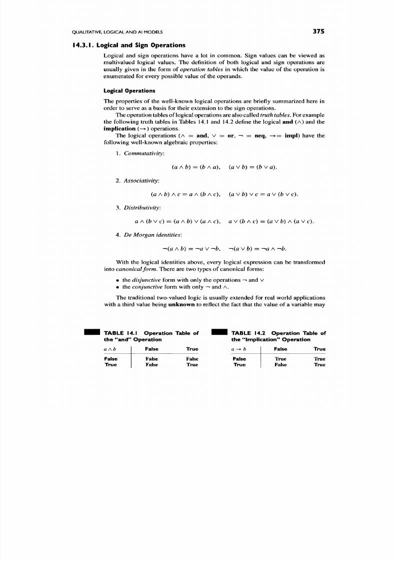
8/17/2019 Process Modelling and Model Analysis-Hangos-Cameron
http://slidepdf.com/reader/full/process-modelling-and-model-analysis-hangos-cameron 392/560
QUALITATIVE. LOGICAL AND Al MODELS
375
14.3.1.
Logical and Sign Operations
Logical and sign operations have a lot in common. Sign values can be viewed as
multivalued logical values. The definition of both logical and sign operations are
usually given in the form of
operation tables
in which the value of the operation is
enumerated for every possible value of the operands.
Logical Operat ions
The properties of the well-known logical operations are briefly summarized here in
order to serve as a basis for their extension to the sign operations.
The operation tables of logical operations are also called
truth tables.
For example
the following truth tables in Tables 14.1 and 14.2 define the logical an d (A) and the
implication (->) operations.
The logical operations (A = and, v = or , -^ = neq, -^ = impl) have the
following well-known algebraic properties:
1.
Commutativity:
{aAb) = {bA a), (av b) = {bv a).
2.
Associativity:
(aAb) Ac = aA{b Ac), (aw b)v c = av (bv c).
3. Distributivity:
a A (b V c) = (a A b) V (a A c), av (b Ac) = (av b) A(av c).
4. De Morgan identities:
-.(fl
Ab) = -^av -^b, -'(a w b) = ^a A
--fo.
With the logical identities above, every logical expression can be transformed
into
canonical
form. There are two types of canonical forms:
• the
disjunctive
form with only the operations -^ and v
• the
conjunctive
form with only -• and A.
The traditional two-valued logic is usually extended for real world applications
with a third value being unknown to reflect the fact that the value of a variable may
TA BL E 14 .1 Op era t i on Tab le o f
t h e " a n d " O p e r a t i o n
aAb
False
True
False True
False
False
False
True
TA BL E 14.2 Op era t io n Tab le o f
t h e ' i m p l i c a t i o n " O p e r a t i o n
b
False
True
False True
True
False
True
True
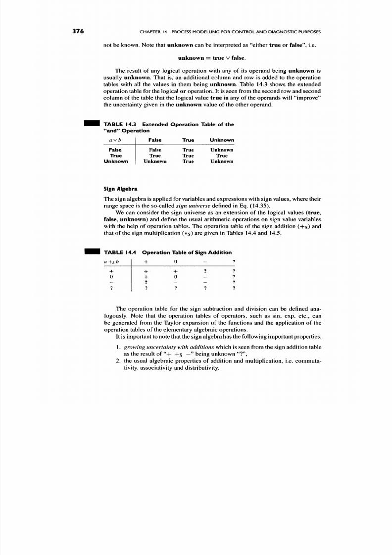
8/17/2019 Process Modelling and Model Analysis-Hangos-Cameron
http://slidepdf.com/reader/full/process-modelling-and-model-analysis-hangos-cameron 393/560
376
CHAPTER 14 PROCESS MODE LLING FOR CO NT RO L AN D DIAGN OST IC PURPOSES
not be known. Note that unknown can be interpreted as "either true or false", i.e.
unknown = true v false.
The result of any logical operation with any of its operand being unknown is
usually unknown. That is, an additional column and row is added to the operation
tables with all the values in them being unknown. Table 14.3 shows the extended
operation table for the logical or operation. It is seen from the second row and second
column of the table that the logical value true in any of the operands will "improve"
the uncertainty given in the unknown value of the other operand.
TA BL E 14.3 Ex tended Op era t io n Tab le o f the
" a n d "
O p e r a t i o n
avb
False True Unknown
False
True
Unknown
False True Unknown
True True True
Unknown True Unknown
Sign Algebra
The sign algebra is applied for variables and expressions with sign values, where their
range space is the so-called sign universe defined in Eq. (14.35).
We can consider the sign universe as an extension of the logical values (true,
false, unknown) and define the usual arithmetic operations on sign value variables
with the help of operation tables. The operation table of the sign addition (-hs) and
that of the sign multiplication (*s) are given in Tables 14.4 and 14.5.
TABLE 14.4
a-\-sb
+
0
—
?
O p e r a t i o n
+
+
+
7
7
Table of
0
+
0
—
?
Sign Addit ion
_ ?
? ?
_ ?
_ 7
?
?
The operation table for the sign subtraction and division can be defined ana
logously. Note that the operation tables of operators, such as sin, exp, etc., can
be generated from the Taylor expansion of the functions and the application of the
operation tables of the elementary algebraic operations.
It is important to note that the sign algebra h as the following important pro perties.
1.
growing uncertainty with additions
wh ich is seen from the sign addition table
as the result of " + + s
—
being unknown "?",
2. the usual algebraic properties of addition and multiplication, i.e. commuta-
tivity, associativity and distributivity.
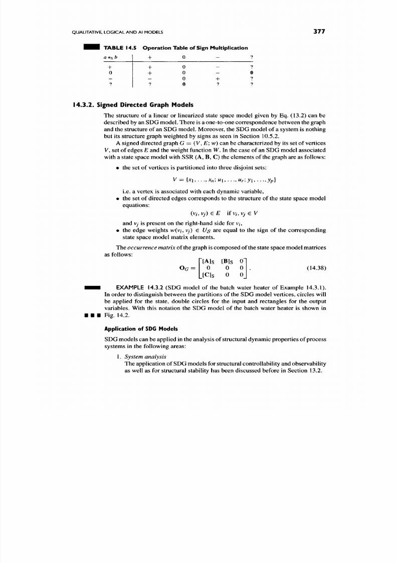
8/17/2019 Process Modelling and Model Analysis-Hangos-Cameron
http://slidepdf.com/reader/full/process-modelling-and-model-analysis-hangos-cameron 394/560

8/17/2019 Process Modelling and Model Analysis-Hangos-Cameron
http://slidepdf.com/reader/full/process-modelling-and-model-analysis-hangos-cameron 395/560
378
CHAPTER 14 PROCESS MODELLING FOR CONTROL AND DIAGNOSTIC PURPOSES
FIGURE 14 .2 Structure digraph of the batch water heater.
2. Qualitative prediction of the unit step response
Using sign algebraic manipulation it is possible to determine [97] the
•
sign of the initial deviation of the step response
by com puting the value of
the shortest path in SDG. The sign value of a path in an SDG is the sign
product of the signs as edge weights forming the directed path.
• sign of the steady state deviation by computing the solution of a linear
sign set of equations corresponding to the steady state algebraic model
equations.
It is important
to
note that because of
the
properties of the sign addition we often
have indeterm inate (denoted by 1) values as qualitative prediction.
EXAMPLE 14.3.3 (Qualitative prediction of the unit step response of the batch
water heater of Example 14.3.1). The SDG m odel of the batch water heater is
shown in Fig. 14.2.
Let us compu te the sign of the initial deviation of the unit step response of output
To (where To is the output temperature variable w hile the state temperature variable
is denoted by
T)
to the unit step in input
K.
The shortest path between
K
and
T
is
(/c, T ), ( r ,
To).
The sign on both of the edges involved is " + " therefore the sign value
of the path is again "-h". This m eans that the initial deviation of the temperature when
putting a positive step chan ge to the binary sw itch of the heater is positive.
14.3.3. Confluences
The notion of confluences as a kind of qualitative model h as been introduced in AI by
de Kleer and Brow n [98] in their theory called "Qu alitative Physics". Confluences
can

8/17/2019 Process Modelling and Model Analysis-Hangos-Cameron
http://slidepdf.com/reader/full/process-modelling-and-model-analysis-hangos-cameron 396/560
QUALITATIVE, LOGICAL AND Al MODELS 379
be seen as sign versions of (lumped) balance equations from a process engineering
perspective.
They can be formally derived from lumped process model equations in the
following steps:
1.
Define qualitative variables
[q]
and 8q to each of the model variables q(t) as
follows:
q^[q]z= sign(^), dq/dt ^ 8q = sign(d^/dO,
where sign (•) stands for the sign of the operand;
2.
operations are replaced by sign operations,
i.e.
+ ~ + S , * ~ *s etc.
3.
parameters are replaced by + or — or 0
forming
sign constants
in the
confluence equations, i.e. they virtually disappear from the equations.
The
solution of a confluence
is computed by simple enumeration of all possible
values of the qualitative variables and arranged in an operation (truth) table of the
confluence.
The operation (truth) table of a confluence contains all the possible v alues
satisfying it and resemb les the operation table for sign operation s.
The above concepts are illustrated on the example of the batch water heater
introduced in Example
14.3.1.
• • • EXAMPLE 14.3.4 (Confluences of the batch water heater of Example 14.3.1).
The confluences are derived from the model eq uations (14 .36 )-( 14.37) in the
following steps:
1.
Qualitative variables
From their physical meaning the sign value of the variables is as follows:
[ ^ / l ] € { 0 , + } , [ r 7 2 ] € { 0 , + ) , M € { 0 , + }
2.
Sign constants
The sign of all parameters is strictly positive, so that all sign constants are
equal to "+".
3.
Confluences
Sh = [m]-s[ri2l (14.39)
8T = [Ti-T]^s[m]-hs[Kl
(14.40)
The truth table of the confluence (14.39) is shown in Table 14.6.
The truth table of the other confluence (14.40) has more columns on the right
hand because we have more variables. Observe that a composite qualitative variable
• • •
[T i — T]
is present in the first right hand column of Table 14.7.
Application of Confluences
The solution of confluences, being various interpretations of the truth table, can be
applied for process monitoring and diagnosis purposes. Some of the characteristic
applications are as follows.
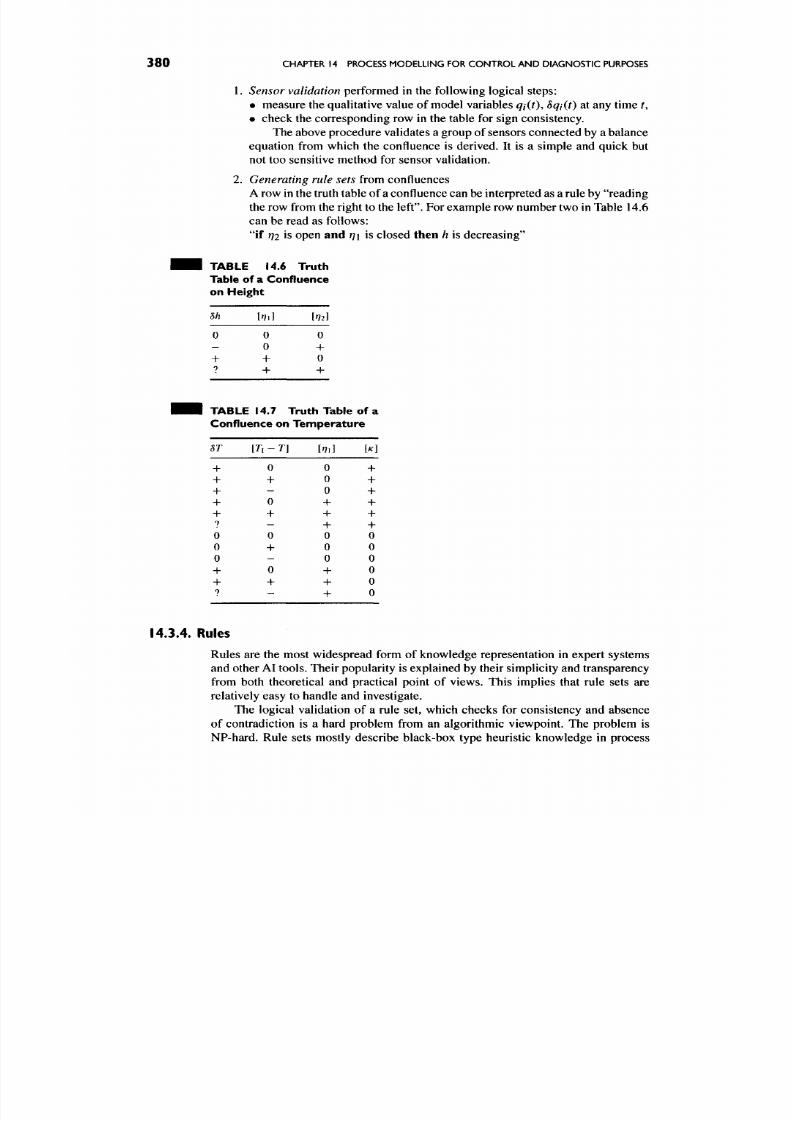
8/17/2019 Process Modelling and Model Analysis-Hangos-Cameron
http://slidepdf.com/reader/full/process-modelling-and-model-analysis-hangos-cameron 397/560
3 8 0 CHAPTER 14 PROCESS MO DELLIN G FOR CO NT RO L A N D DIAG NOS TIC PURPOSES
1. Sensor validation performed in the following logical steps:
• measure the qualitative value of model variables
qtit),
8qi(t) at any time t,
• check the correspon ding row in the table for sign consistency.
The above procedure validates a group of sensors connected by a balance
equation from which the confluence is derived. It is a simple and quick but
not too sensitive m ethod for sensor v alidation.
2.
Generating rule sets
from confluences
A row in the truth table of a confluence can be interpreted as a rule by "reading
the row from the right to the left". For example row number tw o in Table 14.6
can be read as follows:
"if
r]2
is open an d rj \ is closed then h is decreasing"
T A B L E
Table of
14.6
T r u t h
a Conf luence
on He ight
8h
0
-
+
7
[m]
0
0
+
+
im]
0
+
0
+
TABL E 14.7 Tru th Table of a
Confluence on Tem perature
8T
+
+
+
+
+
?
0
0
0
+
+
7
[Ti - T]
0
+
-
0
+
-
0
+
-
0
+
-
Im]
0
0
0
+
-f
+
0
0
0
+
+
+
M
+
+
+
+
4-
+
0
0
0
0
0
0
14.3.4. Rules
Rules are the most widespread form of knowledge representation in expert systems
and other AI tools. Their popu larity is explained by their simplicity and transparency
from both theoretical and practical point of views. This implies that rule sets are
relatively easy to handle and investigate.
The logical validation of a rule set, which checks for consistency and absence
of contradiction is a hard problem from an algorithmic viewpoint. The problem is
NP-hard. Rule sets mostly describe black-box type heuristic knowledge in process
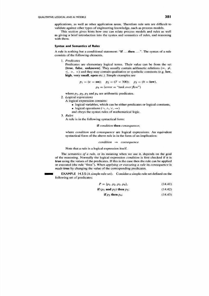
8/17/2019 Process Modelling and Model Analysis-Hangos-Cameron
http://slidepdf.com/reader/full/process-modelling-and-model-analysis-hangos-cameron 398/560
QUALITATIVE. LOGICAL AND Al MODELS 381
applications, as well as other application areas. Therefore rule sets are difficult to
validate against other types of engineering knowledge, such as process models.
This section gives hints how one can relate process models and rules as well
as giving a brief introduction into the syntax and semantics of rules, and reasoning
with them.
Syntax and Semantics of Rules
A rule is nothing but a conditional statement: "if . . . the n . . . " . The syntax of a rule
consists of the following elements.
1.
Predicates
Predicates are elementary logical terms. Their value can be from the set
{ true, false, un kn ow n} . They usually contain arithmetic relations (= , 7^,
< , > , < ) and they may contain qualitative or symbolic constants (e.g. low,
high, very small, open etc.). Simple examples are
p ^
z= {K = on) ; p2 = (T < 300); p^ = (h = low),
P4 = (error = "tank overflow'')
wherep\ ,P2,P3 andp4 are arithmetic predicates.
2.
Logical expressions
A logical expression contains:
• logical variables, which can be either predicates or logical constan ts,
• logical operations
(-1,
A, v,
—>•)
and obeys the syntax rules of mathematical logic.
3.
Rules
A
rule is in the following syntactical form:
if
condition
then
consequence;
where
condition
and
consequence
are logical expressions. An equivalent
syntactical form of the above rule is in the form of an implication:
condition —>• consequence
Note that a rule is a logical expression itself.
The semantics of a rule, or its meaning when we use it, depends on the goal
of the reasoning. Normally the logical expression
condition
is first checked if it is
true using the values of the predicates. If this is the case then the rule can be applied
or executed (the rule "fires")- When applying or executing a rule its consequence is
made
tr ue by changing the value of the corresponding predicates.
• • • EXAMPLE 14.3.5 (A simple rule set). Consider a simple rule set defined on the
following set of predicates:
P=-{PUP2.P3^P4],
(14.41)
if (pi and/72) then /73; (14.42)
if/73then/74; (14.43)
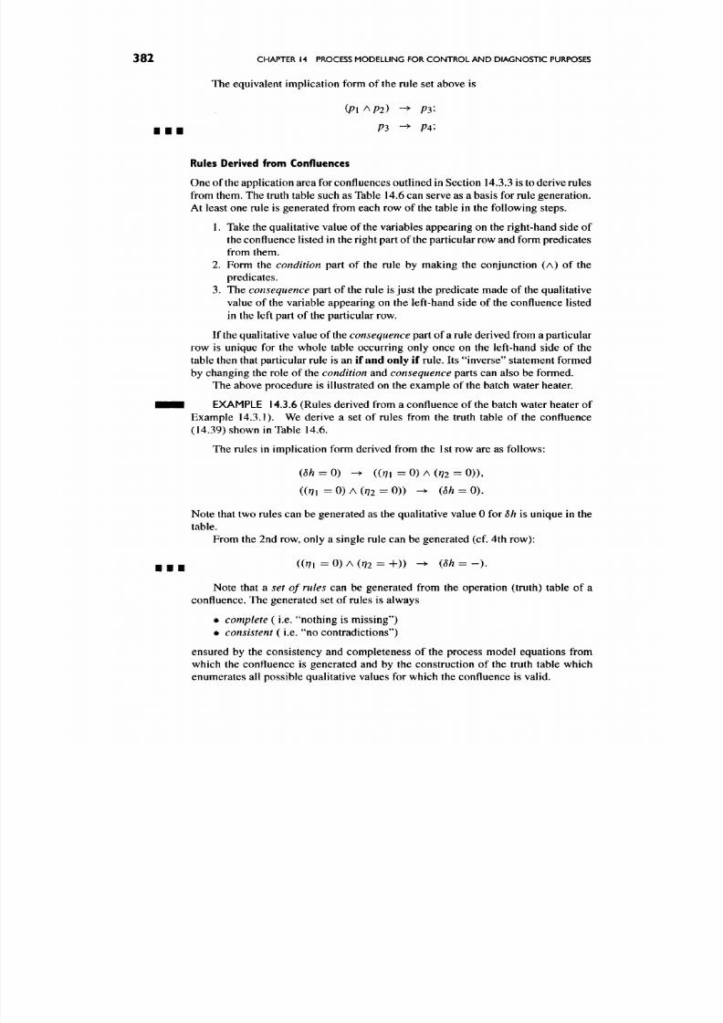
8/17/2019 Process Modelling and Model Analysis-Hangos-Cameron
http://slidepdf.com/reader/full/process-modelling-and-model-analysis-hangos-cameron 399/560
3 8 2
CHAPTER
14
PROCESS MODELLING FOR CONT ROL AN D DIAG NOSTIC PURPOSES
The equivalent implication form of the rule set above is
• • • P3 -^ P4\
Rules Derived from Confluences
One of the application area for confluences outlined in Section 14.3.3 is to derive rules
from them. The truth table such as Table 14.6 can serve as a basis for rule generation.
At least one rule is generated from each row of the table in the following steps.
1. Take the qualitative value of the variables appearing on the right-hand side of
the confluence listed in the right part of the particular row and form predicates
from them.
2.
Form the
condition
part of the rule by making the conjunction (A) of the
predicates.
3.
The consequence part of the rule is just the predicate m ade of the qu alitative
value of the variable appearing on the left-hand side of the confluence listed
in the left part of the particular row.
If the qualitative value of the
consequence
part of a rule derived from a particular
row is unique for the whole table occurring only once on the left-hand side of the
table then that particular rule is an if and only if ru le. Its "inverse" statement formed
by changing the role of the condition and consequence parts can also be formed.
The above proc edure is illustrated on the example of the batch water heater.
EXAMPLE 14.3.6 (Rules derived from a confluence of the batch water heater of
Exam ple 14.3.1). We derive a set of rules from the truth table of the confluence
(14.39) shown in Table 14.6.
The rules in implication form derived from the 1st row are as follows:
{8h = 0) -^ ((r/i = 0) A (;72 = 0) ),
((r/l = 0) A ( 72 = 0)) - ^ (5/1 = 0).
Note that two rules can be generated as the qualitative value 0 for
8h
is unique in the
table.
From the 2nd row, only a single rule can b e generated (cf. 4 th row):
((^1 = 0) A (r?2 = + ) ) ^ ((5ft = - ) .
Note that a set of rules can be generated from the operation (truth) table of a
confluence. The generated set of rules is always
# complete (i.e. "nothing is missing")
•
consistent
(i.e. "no contradictions")
ensured by the consistency and completeness of the process model equations from
which the confluence is generated and by the construction of the truth table which
enumerates all possible qualitative values for wh ich the confluence is valid.

8/17/2019 Process Modelling and Model Analysis-Hangos-Cameron
http://slidepdf.com/reader/full/process-modelling-and-model-analysis-hangos-cameron 400/560
QUALITATIVE, LOGICAL AND Al MODELS 383
Reasoning with Rules
Rules are used for reasoning in intelligent systems, mainly in expert systems. The
data base of
an
expert system is called the knowledge base and it consists of
two
main
parts:
• a static part
(relations)
containing the rules in encoded form,
• a dynamic part (facts) where the changing values of the predicates are stored.
The value of all predicates forms the state of the knowledge base. This state is
described by a point in the so caWtd
predicate space
spanned by all predicates:
V = {[puP2,
. . . , p p f I
Pi e
{true, false}},
where
P
is the number of all predicates.
The reasoning is performed by executing the rules which are applicable, i.e. those
which "fire'\
Formally, for a rule in the form of
condition -> consequence,
the execution performs the following manipulation:
if (condition = true) then (consequence := true).
Note that one moves in the predicate space by executing rules as the value of the
predicates appearing in the
consequence
are changed by executing the rule. The part
of the expert system performing the reasoning is called the inference engine.
There can be more than o ne applicable rule in a situation. Th is is called a
conflict
situation and various heuristic techniques can be applied to select the rule to be
executed from them for
conflict resolution.
It is an important property of a given
inference engine as to which conflict resolution techniqu es are applied and how these
techniques can be tuned according to the need of the particular application.
There are two different methods for reasoning with rules driven by the reason-
ing goal:
1.
Forward chaining used for prediction
Here the task
is
toflnd all consequences of the facts (i. e. set of predicate values)
by executing the rules in their normal direction,
reasoning from
conditions
to
consequences.
2. Backwa rd chaining
used for diagnosis
Here one wants toflnd all causes of the facts (i.e. set of predicate values) by
using the rules opposite to the normal direction.
The following simple example shows the principles of forward and backward
chaining.
• • • EXAMPLE 14.3.7 (Reasoning with the simple rule set of Exam ple 14.3.5). Con
sider a simple rule set given in Eqs. (14.42) and (14.43) based on the predicate set
(14.41).
First we classify the predicates in the set P according their place in the rules:
the "root" predicates are the ones which only occur on the
condition
part of the rules.
In our case they are:
^root = {P\.P2\'
8/17/2019 Process Modelling and Model Analysis-Hangos-Cameron
http://slidepdf.com/reader/full/process-modelling-and-model-analysis-hangos-cameron 401/560
384
CHAPTER
14
PROCESS MODELLING FOR CONTR OL AND DIAGNOSTIC PURPOSES
The root predicates should have values determined by the outside world, that is from
measurements before we start reasoning with forward chaining.
Forward
chaining
Let us assum e we have the following values for the root predicates:
pi = true, p2 = true
and all the other predicates have unknown values. Then rule (14 .42) fires and we get
P2 =
true by executing it. Now rule (14.43) fires and gives p4
=
true after execution.
Backw ard chaining
Now we assume no value for the root predicates:
p \
= unknown,
p2 =
unknown,
but a definite value for the predicate p^
P4 = true, /73 = unk now n.
First, we use rule (14.43) where we have the consequence part defined and we get
/73 = true by backward executing it. Now rule (14.42) is applicable for backward
• • • reasoning and gives p i = true andp2 = true after execution.
14.4. SUMMARY
The question of model applications in a range of control scenarios is investigated in
this chapter covering such tech niques as LQR and model predictive control. The form
and use of the model is illustrated in these applications.
The second part of this chapter looks at typical models applied to the problem
of process diagnosis. This is an important aspect of model development and process
engineering.
Finally, dynamic process models with interval-valued variables are discussed
which are the form of process m odels applicable to intelligent control and diagn osis.
These models take various forms ranging from qualitative models through to rule
based representations.
14.5.
FURTHER READING
The area of chemical process control is a broad and rapidly developing one with books,
conferences and journ als entirely devoted to it. Here, dynamic proc ess mod elling has
been w idely recogn ized as one of the key areas. Therefore, we do not attempt to m ake
a literature review on this broad topic from the process modelling point of view but
direct the readers ' attention to the most imp ortant information sources. Note that the
information sources for process control are overlapping with that of model analysis.
8/17/2019 Process Modelling and Model Analysis-Hangos-Cameron
http://slidepdf.com/reader/full/process-modelling-and-model-analysis-hangos-cameron 402/560
APPLICATION EXERCISES 385
therefore we also refer to the sources given in Section 13.5. Further information
sources are:
• y^eb
Control Engineering Virtual Library, with homepage:
http://www-control.eng.cam.ac.uk/extras/Virtual_Library/
Control_VL.html
• Textbooks
There are a few special textbooks available on process control for those who
have process engineering background such as [99 -10 1].
14.6. REVIEW QUESTIONS
Q14.1.
Give the problem statement of pole-placement control. What are the
conditions for its application? W hat are the properties of the controller? (Section 14.1)
Q14.2.
Give the problem statement of the LQ R. Wh at are the conditions for its
application? W hat are the properties of the controller? Why is state filtering important
in process control? (Section 14.1)
Q14.3. Give the problem statement of model-based predictive control. What are
the conditions for its application? What are the steps of its conceptual solution?
(Section 14.1)
Q14.4. Give the problem statem ent of prediction-based d iagno sis. W hat are the steps
in its conceptual solution? (Section 14.2)
Q14.5. Give the problem statemen t of identification-based diagno sis. W hat are the
steps in its conceptual solution? (Section 14.2)
Q14.6. Com pare the logical and sign operations Wh at are the similarities and dif
ferences? What are the strength and weaknesses of logical and AI methods which are
based on them? (Section 14.3)
Q14.7. Com pare the SDG mode l, the confluences and the rule-set derived from the
confluences of the same lumped process model. What is the relation between them?
What are the similarities and differences? Is there any one-to-one relation among
them? (Section 14.3)
14.7. APPLICATION EXERCISES
A14.1. Is the pole placement controfler applicable for stabilizing the state space
model (Eqs. (14.36) and (14.37)) of the batch water heater? Why? Formulate the
special case of the LQR controller design to stabilize the model. (Section 14.1)
A14.2. Derive the confluences from the nonlinear state space mod el of a CSTR
derived in Example 10.3.1 in Section 10.4. Give the truth table of the confluences.
(Section 14.3)
A
14.3.
Derive the com plete set of rules for both of the confluences o btained in the
previous Exercise (A14.2). Which are the rows in the truth tables giving rise to two
rules (in both direction)? (Section 14.3)

8/17/2019 Process Modelling and Model Analysis-Hangos-Cameron
http://slidepdf.com/reader/full/process-modelling-and-model-analysis-hangos-cameron 403/560
386
CHAPTER
14
PROCESS MODELLING FOR CO NTR OL AND DIAG NOSTIC PURPOSES
A14.4. Derive the com plete set of rules for the truth Table 14.6. W hat are the
properties of that rule set and why ? (Section 14.3)
A14.5. Derive the comp lete set of rules for the truth Table 14.7. Is this set complete?
How would you show this? (Section 14.3)
A14.6. Apply forward chaining reasoning with the rule set of Example 14.3.5
assuming the following values of the root predicates
pi
=z
true, p2 = false
(Section 14.3)
A14.7. Apply backward c haining reasoning with the rule set of Exam ple 14.3.5
assuming the following values of the predicates
p \ =
false,
p2 =
unknown
P3 = unknown, p^ = false
Is your result unique? Why? (Section 14.3)

8/17/2019 Process Modelling and Model Analysis-Hangos-Cameron
http://slidepdf.com/reader/full/process-modelling-and-model-analysis-hangos-cameron 404/560
MODELLING DISCRETE EVENT
SYSTEMS
This chapter discusses the modelling and model analysis issues related to discrete
event dynamic systems applied in process systems engineering. The term
discrete
event system [102] stands for dynamic systems with discrete valued variables: state,
input and output variables with a finite number of possible values. Time is also
considered to be discrete in discrete event systems but the time instances are not
necessarily equidistant. An "event" occurs when any of the discrete valued variables
change their value, and this generates a discrete time instance.
The theory of discrete event systems has been developed within systems and
control theory and computer science where most of the applications are found.
The material presented in this chapter is arranged as follows:
• The characteristic properties and the application areas of discrete event systems
in process systems engineering are briefly outlined in Section 15.1.
• The most impo rtant approac hes to mod el representation are introduced and
compared in Section 15.2.
• The solution of discrete event dyna mic mo dels performed via discrete event
simulation is the subject of Section 15.3.
• Finally, the most important properties of discrete event systems, and tools for
analysing these properties, are described in Section 15.4.
It is important to note here that process system s are most often com posed
of both
discrete and continuous subsystems. Chapter 16 deals with these so-called hybrid
systems.
387

8/17/2019 Process Modelling and Model Analysis-Hangos-Cameron
http://slidepdf.com/reader/full/process-modelling-and-model-analysis-hangos-cameron 405/560
3 8 8 CHAPTER 15 MODELLING DISCRETE EVENT SYSTEMS
15 .1 .
CHARACTERISTICS AND ISSUES
Process systems are often influenced by external or internal events which o ccur instan
taneously and often have a discrete range space. In other words, they may take only
a finite number of possible values. Binary on/off or open/close valves, switches or
operator actions are the simplest examples of external discrete events. Rapid phase
chang es, such as sudden evaporation or condensation are examples of internal events.
Som e of the more complex n onlinear behaviour like weeping or flooding n distillation
columns may also be viewed as internal discrete events.
If one is only interested in describing the behaviour of
a
process system to cover
events that influence it and the subsequent event sequences which may arise then
some kind of discrete event process system model is used. Such a discrete event
model focuses only on the sudden discrete changes and approximates the continuous
behaviour of the continuous system elements by event sequences. From a system
theoretic point of view all variables including the state, input and output variables
of the process system are then described by time-dependent variables with discrete
range space:
^(0 e X = {^0, - ^ 1 , . . . ,
Xn], M (0
€ U =
[uo,
Ml,..., M,J,
j ( 0 € Y = { j o , J l , . . . , J n } . (15.1)
Here, the elements in the range space or the possible discrete values of the variables
can be either numerical values or disjunct intervals or even symbolic values. In this
sense there is a close relationship between discrete event and qualitative dynamic
models.
A chan ge in the discrete value of any of the variables is called an event. With the
operation of a discrete event system its variables change their values in time causing
sequences of events. The set of all discrete time of these events forms the discrete
time domain of the system.
Discrete event process system models naturally arise in the following application
areas:
1. Discrete event process system models are traditionally and effectively used
in design, verification and analysis of operating procedures which can be
regarded as sequences of external events caused by operator interventions.
2.
The
scheduling and plant-wide control of batch process plants
is another
important, popular and rapidly developing field.
15.2. APPROACHES TO MODEL REPRESENTATION
There are various related approaches to describe a discrete event dynamic system
with discrete time and discrete valued variables.
Most of the approaches representing such systems use combinatorial or finite
techniques. This means that the value of the variables including state, input and
output variables, are described by finite sets and the cause-consequen ce relationships
between these discrete states are represented by directed graphs of various kinds.
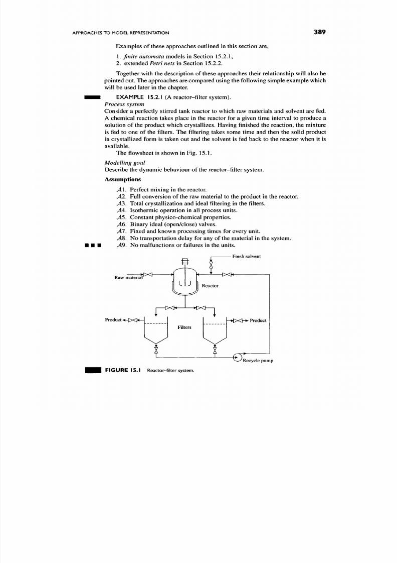
8/17/2019 Process Modelling and Model Analysis-Hangos-Cameron
http://slidepdf.com/reader/full/process-modelling-and-model-analysis-hangos-cameron 406/560

8/17/2019 Process Modelling and Model Analysis-Hangos-Cameron
http://slidepdf.com/reader/full/process-modelling-and-model-analysis-hangos-cameron 407/560
390
CHAPTER
15
MODELLING DISCRETE EVENT SYSTEMS
15.2.1. Finite Automata
The notion of finite automata is a basic and central one in computer science for
analyzing algorithmic (computational) complexity [69]. A famous example is the
so-called Turing machine of which various types exists.
A finite automata is an abstract discrete machine with at least one input tape
containing symbols from a predefined finite set called an alphabet. The automata
operates in discrete steps and it has a predefined set of states. When performing a
step the automata changes its state depending on its current state and the subsequent
symbol, read from the input tape. Thereafter, it may or may not move the reading
head of the input tape one step ahead. This instruction to move or not to move the
head is encoded in the state-symbol pair before the step.
The above abstract operation is formally described as follows. The finite automata
is a triplet
A = ( e , ^ , 5 ) , (1 5.2 )
where Q is the finite set of discrete states in the automata. The state of the reading
head (w hether it is to be moved or not to be mov ed) is also encoded in the state of the
automata. E is a finite set of input alphabet. This set may contain a special symbol
"#" denoting the end of the tape. The input alphabet set is used in the automata to
describe external events, as will be explained in more detail later in Section 15.2.3
and
8
is the state transition function of the finite automata, w hich determines the next
state, after a symbol from the input tape has been read. Formally,
(5 : G X E -> G. (15.3)
This is normally a partial function, defined only for some of the state-symbol pairs.
Note that bounded Petri nets (in Section 15.2.2) can also be described by this set
of states, considering the nodes in the related reachability graph as states.
The state transition function is visualized using the so called state transition
graph, which is a weighted directed graph GA = (V^^EA', W ^ ) , where VA is the set
of vertices,
EA
is the set of edges with edge weights w^. The vertices of the state
transition graph are the discrete states, that is VA = Q. There is a directed edge
between two vertices if the state transition function is defined for the starting state
vertex of the edge resulting in the ending state vertex of the edge for some symbol on
the input tape. The symbol is put onto the edge as its edge weight.
In order to describe the operation of the automata, we need to define special
subsets of discrete states: Qi the set of admissible initial states g i c Q and g p the
set of final states gp ^
Q-
The autom ata can be started from an initial state with the given "c ontent" of the
input tape. It works according to the state transition function 8 until it reaches a final
state from set QF» and then it stops. The autom ata may also stop if the state transition
function 8 is not defined for a particular (Qy, Sj) pair or when it reaches the end of
the input tape (denoted by the end of tape symbol "#"). Finally, the automata may go
into an "infinite cy cle", and never stop.
Note that in a finite automata m odel, there are only discrete time steps without any
duration. It means that only precedenc e or cause-con sequ ence relations are modelled.
The ideas are best understood if one considers a simple everyday example:
a hot/cold drink automata.
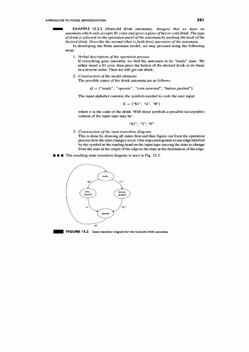
8/17/2019 Process Modelling and Model Analysis-Hangos-Cameron
http://slidepdf.com/reader/full/process-modelling-and-model-analysis-hangos-cameron 408/560
APPROACHES TO MODEL REPRESENTATION 391
• • • EXAMPLE 15.2.2 (Hot/cold drink automata).
Imagine that we have an
automata w hich only accepts $1 coins and gives a glass of hot or cold
drink.
The type
of drink is selected on the operation panel of the automata
by
pushing the knob of the
desired
drink.
Describe the normal (that is fault-free) operation of the autom ata.
In developing the finite automata model, we may proceed using the following
steps:
1. Verbal
description of the operation process
If everything goes smoothly we find the automata in its "ready" state. We
either insert a $1 coin, then press the button of the desired drink or do these
in a reverse order. Then we will get our drink.
2.
Construction of the model elements
The possible states of the drink automata are as follows:
Q
=
[''ready\ ''operate'', "coinJnserted'\ ' 'button-pushed'']
The input alphabet contains the symbols needed to code the user input:
E = {"$1",
"n",
"#"}
where
n
is the code of the drink. With these symbols a possible (acceptable)
content of the input tape may be:
"$1" , " 3 " , " # "
3. Construction of the state transition diagram
This is done by drawing all states first and then figure out from the operation
process how the state changes occur. One step corresponds to one edge labelled
by the symbol at the reading head on the input tape causing the state to change
from the state at the origin of the edge to the state at the destination of the edg e.
• • • The resulting state transition diagram is seen in Fig. 15.2.
F I G U R E 1 5 . 2 State transition diagram for the hot/cold drink automata.
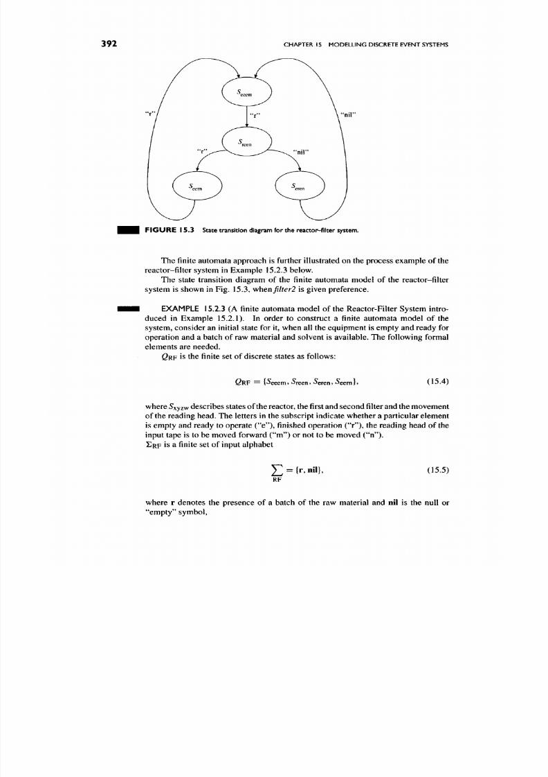
8/17/2019 Process Modelling and Model Analysis-Hangos-Cameron
http://slidepdf.com/reader/full/process-modelling-and-model-analysis-hangos-cameron 409/560
392
CHAPTER 15 MODELLING DISCRETE EVENT
SYSTEMS
FIGURE 15 .3 State transition diagram for the reac tor-filter system.
The finite automata approach is further illustrated on the process ex ample of the
reactor-filter system in Example 15.2.3 below.
The state transition diagram of the finite automata model of the reactor-filter
system is shown in Fig. 15.3, ^hen filter is given preference.
EXAMPLE 15.2.3 (A finite autom ata model of the Reacto r-Filter System intro
duced in Example 15.2.1). In order to construct a finite automata model of the
system, co nsider an initial state for it, when all the equipment is empty and ready for
operation and a batch of raw material and solvent is available. The following formal
elements are needed.
QRF is the finite set of discrete states as follows:
G R F
— {' eeem» •^reen? 'Jeren» »^eem}»
(15.4)
where 5xyzw describes states of the reactor, the first and second filter and the movement
of the reading head. The letters in the subscript indicate w hether a particular elem ent
is empty and ready to operate ("e")» finished operation ("r"), the reading head of the
input tape is to be moved forward ("m") or not to be moved ("n").
ERF
is a finite set of input alphabet
5;^ = {r,nil},
(15.5)
RF
where r denotes the presence of a batch of the raw material and nil is the null or
"empty" symbol.

8/17/2019 Process Modelling and Model Analysis-Hangos-Cameron
http://slidepdf.com/reader/full/process-modelling-and-model-analysis-hangos-cameron 410/560
APPROACHES TO MODEL REPRESENTATION 393
^RF is the State transition function of the finite automata
^RF (^eeem, r) = 5'reen, (1 5. 6)
^RF (' reen, r) = ^ eem, (1 5. 7)
^RF(5^reen, ni l) = Seren, (1 5. 8)
^RF (' eem. r ) = 5'eeem» (1 5. 9)
^RF ( S'eren, ni l) = Seeem • (15.10)
Ql is the finite set of initial states
Ql — {•J'eeem}
Q F is the finite set of final states
• • • G F = {'S'eeem}.
15.2.2.
Petri Nets
Petri nets were originally developed for modelling sequences of finite automata and
have been found to be useful for simulation and analysis of resource allocation
problems of discrete event dynamic systems with both sequential and parallel ele
ments. There are a number of extensions to the original concept of Petri nets in the
literature including timed, hierarchical, multi-valued logical as well as stochastic
elements [103,104].
The main application area in process engineering is the modelling and ana
lysis of batch process systems and that of specifying/describing operating pro
cedures [105,106].
Low Level Petri Nets: Structure and Dynamics
A Petri net model of a discrete event dynamic system represents its possible (discrete)
states and the state changing events that relate to them.
An event can only occur if
its preconditions described by a particular discrete value of the system state holds.
The occurrence of an event changes the state of the system into the post-conditions
or consequences of the event. In a Petri net structure, the states or their values as
conditions are generalized to the notion of
places,
and events are described by so
called transitions.
The structure of a low level Petri net
is formally described by the following
four-tuplet:
C = ( P , T , I , 0 ) , (1 5.1 1)
where P = { p i , . . . , /7„} is the non-empty finite set of places, T = { fi ,. .. , r,„} is the
non-em pty finite set of transitions, I : T ->• P ^ is the input function relating places
to a transition forming its pre-condition and O : T -> P ^ is the output function
relating places to a transition forming its post-condition or consequence.
Note that the input and output functions give the logical relationships between
places and transitions. In the general case, a place may appear in the pre-conditions
8/17/2019 Process Modelling and Model Analysis-Hangos-Cameron
http://slidepdf.com/reader/full/process-modelling-and-model-analysis-hangos-cameron 411/560
394 CHAPTER 15 MODELLI NG DISCRETE EVENT SYSTEMS
or post-conditions of a transition several times (in m ultiplication) that is denoted by
the symbol P ^ .
The structure
of a Petri net is
usually
described in a graphical way in the form
of a bipartite directed graph Gp
=
(Vp,Ep) because the set of places and that of
transitions are disjoint, that is
pn T
=
id.
The vertex set Vp of the graph is composed of the set of places and that of transitions:
Vp=PUT.
Places are denoted by circles and transitions by bold intervals on the graph.
The input and output functions correspond to the directed edges in the graph.
Because of the bipartite nature of the graph, edges join place-transition pairs only.
A directed edge (p/,
tj )
or
{tj.po)
exists if/?/ is present in the pre-conditions orp^ is
present in the post-conditions of the transition
tj ,
formally
(p/,
tj )
e
E p if Pi
e
I(fy),
(tj.po)
eEp if/70
eO {tj) .
Note that the formal and graphical d escription is fully equivalent.
The formal and graphical description of a simple Petri net structure is given in
the following example.
• • • EXAMPLE 15.2.4 (Formal description of a simple Petri net structure). The
graphical description of the Petri net structure is shown in both of the sub-figures
of Fig. 15.4.
The equivalent formal description is as follows:
Cs
= iPs,Ts,ls.Os\
(15.12)
where
P5 =
{Prr^PsT^PRr,
Ppr]
T5
=
Ur,^R}
l5(^r)
=
[Prr.Psr]
h(fR) = {PRr^PRr)
O sitr) ={pRT,PRr}
O s{tR)
=
{ppr,Psr]
Observe that the graph in Fig. 15.4 contains multiple edges directed to and from the
place /7Rr. This means that the condition c orresponding to place pRr appears twice in
• • • the pre-condition of
^R
and in the post-condition of
tr.
The dynamics
or
operation
of
a Petri net is described using the notion
of markings.
A discrete state of the process system described by a Petri net is represented by the
state of the places, i.e. by the state of conditions.
Aplace may be active with its
associated condition fulfilled or passive when it is not. Atoken is put in a place

8/17/2019 Process Modelling and Model Analysis-Hangos-Cameron
http://slidepdf.com/reader/full/process-modelling-and-model-analysis-hangos-cameron 412/560
APPROACHES TO MO DEL REPRESENTATION
395
^|. "fires"
FIGURE 15 .4 Simple Petri net
when it is active.
A m arking is then a com plete set of the states of the places, or the
distribution of the tokens on places in the Petri net.
The graphical represe ntation of the above example shown in Fig. 15.4 illustrates
the notion of markings by giving two examples. The marking on the left-hand sub-
figure corresponds to the case when the places prr and psr are active.
The engineering interpretation of a marking is based on the meaning of a token
put on a place which can be given in two alternative ways:
1.
Workpiece-based interpretation
We can imagine a token as a workpiece put on a plate (the place) waiting for
further processing performed by a place processing equipment (a transition).
This is the usual interpretation in the manufacturing industries.
2.
Value-based interpretation
We can also associate a logical variable w ith a place. The presenc e of a token
indicates its logical "true" value. The place then represents an event described
by a logical expression, for example the event of
temperature
> 25°C.
The formal description of a marking is performed by constructing an integer-
valued marking function over the set of places
as follows:
/x : P - > A/*, ^JL(pi) = fJLi > 0 ,
fjj = [ / x i , / i 2 , . . . , / ^ / 2 ] , n = |P| ,
(15.13)
(15.14)
where p.(pi) is the number of tokens on the place/?/.
The graphical representation of a marking
is shown on the directed bipartite
graph of the Petri net. The presence of a token on a place is indicated by drawing a
bold dot inside the circle representing the place.
The execution of a Petri net with a given marking
represents one step in the
dynamic state change of the discrete event dynamic system. The state of the system
8/17/2019 Process Modelling and Model Analysis-Hangos-Cameron
http://slidepdf.com/reader/full/process-modelling-and-model-analysis-hangos-cameron 413/560
396 CHAPTER 15 MODELLING DISCRETE EVENT SYSTEMS
is represented by a specific marking. When an event occurs then we say that the
corresponding transition fires. If the precon ditions of a transition tj hold in a marking
/x ' then the event (or transition) tj takes place (that is tj fires) to give rise to a
new marking
ii^''^^\
The preconditions of the transition become false and its post
conditions become true. This m eans that the places connec ted to the firing transition
as preconditions may become inactive and the places connected to the transition as
post-conditions will be active. In notation, we write
[/'Htj >
j / ' - ^ ^ ^ (15.15)
for the event of firing the transition tj.
The graphical representation of the execution is shown in the directed bipartite
graph representation of the Petri net by moving the corresponding token s around the
firing transition. O ne token from each of the precondition places (those with an arrow
directed towards the transition) is taken away and one token is inserted in each of the
post-condition places (those with an arrow directed from the transition).
The formal and graphical description of the execution of a simple Petri net
introduced in Exam ple 15.2.4 is as follows.
• • • EXAMPLE 15.2.5 (Execution of a simp le Petri net of Examp le 15.2.4). The
graphical description of firing transition
tr
is shown in the sub-figures of Fig. 15.4.
The m arking before the firing is drawn on sub-figure (a), while the marking after the
firing is on sub-figure (b).
The situation depicted in sub-figure (a) can be interpreted as follows: we have the
solvent ready (token on the place/7sr) and the reagent(s) ready (token on the place prr).
After finishing the filling (described by the transition
tf )
we have both components
in our equipment ready for further processing (two tokens on place pRr) shown in
sub-figure (b).
The equivalent formal description is as follows:
/f j = [Mrr, Msr, MRr, Mpr], (15.16)
M^ >^ = [ 1 , 1 , 0 , 0 ], (15.17)
/£^*>'r = [ 0 , 0 , 2 ,0 ], (15.18)
• • • /£^ [rr > M^^^ (15.19 )
A finite or infinite sequence of operations is a sequence of the steps of execution
connected by joint markings, i.e.
ix^%, > ii^%j, > . . . [tj, > /£ ^+^>. (15.20)
The marking or the state of the Petri net /x^^"^^^ is called reachable
from
marking
fi^^^ if there is a sequence of transitions forming a finite sequence of operations abov e
moving the net from the state /i^^^
to fi^^^^K
It is important to note that there can be more than one transition able to fire
for a given marking or state of the Petri net. This marking may have more than one
subsequent marking. The fireable transitions can be executed in parallel, when they
do not have any joint place in their preconditions, or they are in conflict. There are
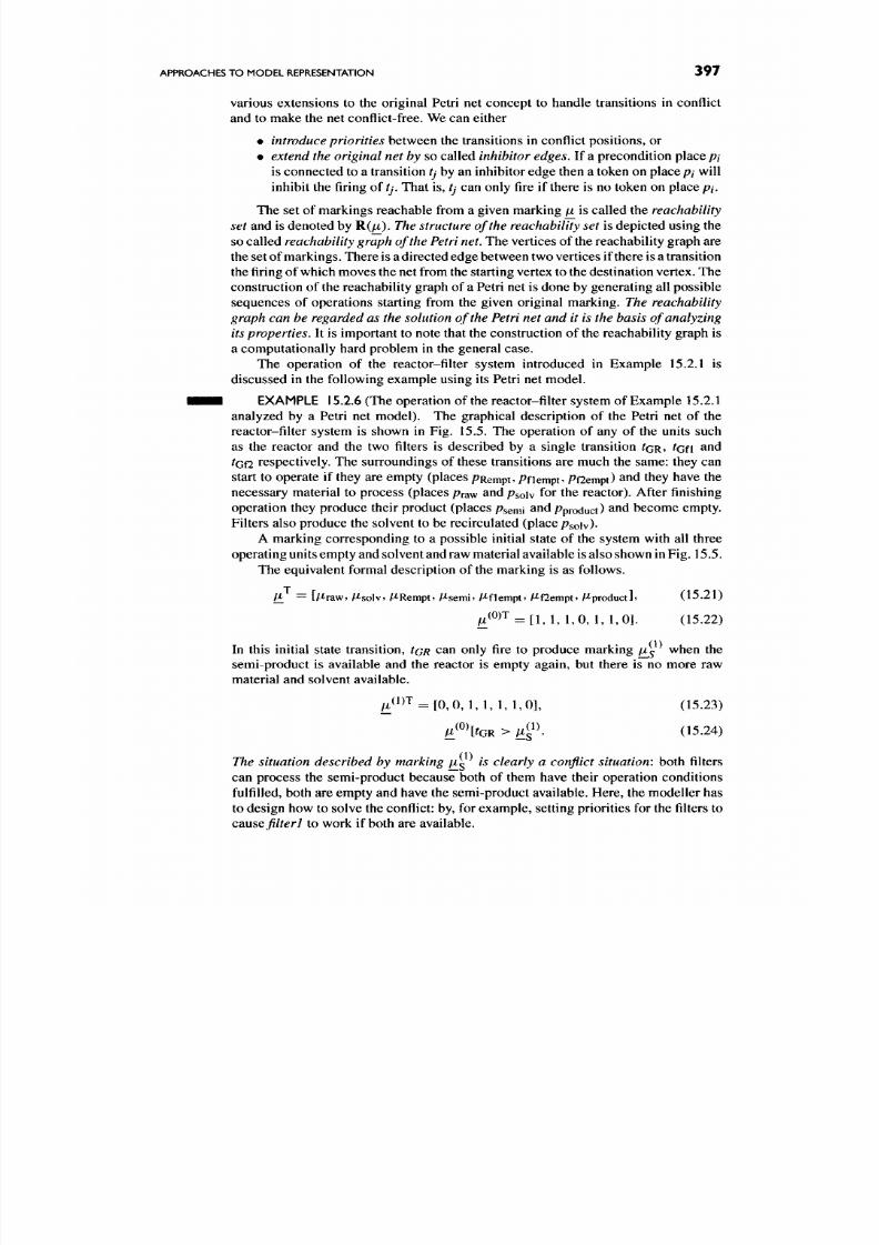
8/17/2019 Process Modelling and Model Analysis-Hangos-Cameron
http://slidepdf.com/reader/full/process-modelling-and-model-analysis-hangos-cameron 414/560
APPROACHES TO MODEL REPRESENTATION 397
various extensions to the original Petri net concept to handle transitions in conflict
and to make the net conflict-free. We can either
• introduce priorities between the transitions in conflict positions, or
•
extend the original net by
so called
inhibitor edges.
If a precondition place
pi
is connected to a transition tj by an inhibitor edge then a token on place pi will
inhibit the firing of tj. That is,
tj
can only fire if there is no token on place /?/.
The set of marking s reachable from a given marking /x is called the
reachability
se t and is denoted by R(/x). T he structure of the reachability set is depicted using the
so called
reachability graph of the
Petri
net.
The vertices of the reachability g raph are
the set of marking s. There is a directed edge betw een tw o vertices if there is a transition
the firing of which moves the net from the starting vertex to the destination vertex. T he
construction of the reachability graph of a Petri net is done by generating all possible
sequences of operations starting from the given original marking.
The reachability
graph can be regarded as the solution of the Petri net and it is the basis of analyzing
its
properties.
It is impo rtant to note that the construction of the reachability graph is
a computationally hard problem in the general case.
The operation of the reactor-filter system introduced in Example 15.2.1 is
discussed in the following example using its Petri net model.
• • • EXAMPLE 15.2.6 (The operation of the reactor-filter system of Example 15.2.1
analyzed by a Petri net mo del). The graphical description of the Petri net of the
reactor-filter system is shown in Fig. 15.5. The operation of any of the units such
as the reactor and the two filters is described by a single transition ^GR, ^Gfl
^^^
tQfi respectively. The surroundings of these transitions are much the same: they can
start to operate if they are empty (places
PRempu
Pflempt*
Pflempt)
^^^
they have the
necessary material to process (places praw and psoiv for the reactor). After finishing
operation they produce their product (places Psemi and /^product) and become empty.
Filters also produce the solvent to be recirculated (place psoiv)-
A marking corresponding to a possible initial state of the system with all three
operating units em pty and solvent and raw m aterial available is also shown in Fig. 15.5.
The equivalent formal description of the marking is as follows.
/£ = LMraw? Msolv» MRempt? Msemi» Mflempt? Mf2empt» /^product]> (15 .2 1)
^ ( 0 ) T ^ [ 1 1 1 0 , 1 , 1 , 0 ] . ( 15 .2 2 )
In this initial state transition, tcR can only fire to produce marking p^ when the
semi-product is available and the reactor is empty again, but there is no more raw
material and solvent available.
/£(l)T = [0 ,0 ,1 ,1 ,1 ,1 ,0 ] , (15.23)
/£^^^[feR>M^^^ (15.24)
The situation described by marking p^ is clearly a conflict situation:
both filters
can process the semi-product because both of them have their operation conditions
fulfilled, both are empty and have the semi-produ ct available. Here, the mod eller has
to design how to solve the conflict: by, for exam ple, setting priorities for the filters to
causQ filter
to work if both are available.
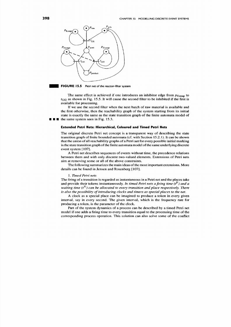
8/17/2019 Process Modelling and Model Analysis-Hangos-Cameron
http://slidepdf.com/reader/full/process-modelling-and-model-analysis-hangos-cameron 415/560
398
CHAPTER 15 MO DEL LING DISCRETE EVENT SYSTEMS
^Rempt( #
0^raw ^
F IG U R E 15.5 Petri net of
the
reactor-filter system
The same effect is achieved if one introduces an inhibitor edge from Pfiemp to
ton
as shown in Fig. 15.5. It will cause the seco nd filter to be inhibited if the first is
available for pro cessing.
If we use the second filter when the next batch of raw material is available and
the first otherwise, then the reachability graph of the system starting from its initial
state is exactly the same as the state transition g raph of the finite automata mo del of
the same system seen in Fig. 15.3.
Extended Petri Nets: Hierarchical, Coloured and Timed Petri Nets
The original discrete Petri net concept is a transparent way of describing the state
transition graph of finite bounded autom ata (cf. with Section 15.2.1). It can be shown
that the union of all reachability graphs of a Petri net for every po ssible initial marking
is the state transition graph of the finite automata model of the same underlying discrete
event system [107].
A Petri net describes sequences of events without time, the precedence relations
between them and with only discrete two-valued elements. Extensions of Petri nets
aim at removing some or all of the above constraints.
The following summ arizes the main ideas of the most important extensions. M ore
details can be found in Jensen and Rosenberg [107].
1. Timed Petri
nets
The firing of a transition is regarded as instantaneous in a Petri net and the places take
and provide their tokens instantaneously.
In timed Petri nets a firing time (t^) and a
waiting time (t^) can be allocated to every transition and place respectively. There
is also the possibility of introducing clocks and timers as special places to the net.
A clock as a special place can be imagined to produce a token in every given
interval, say in every second. The given interval, which is the frequency rate for
producing a token, is the parameter of the clock.
Part of the system dynamics of a process can be described by a timed Petri net
model if one adds a firing time to every transition equal to the processing time of the
corresponding process operation. This solution can also solve some of the conflict
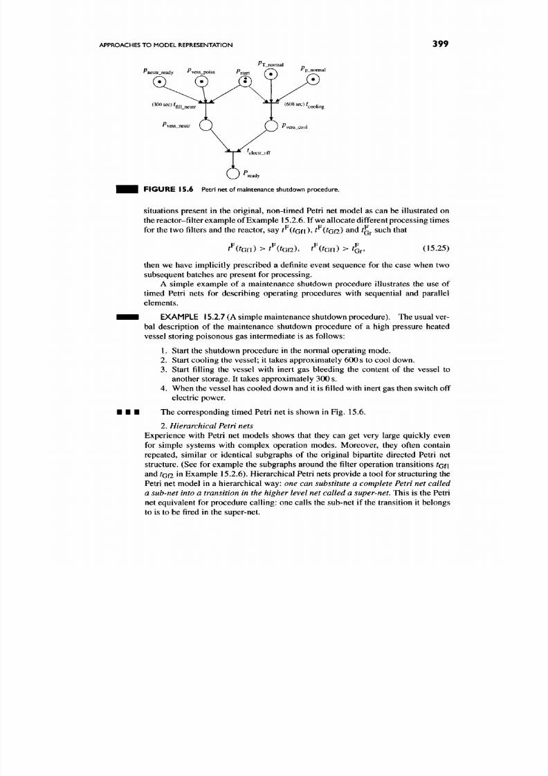
8/17/2019 Process Modelling and Model Analysis-Hangos-Cameron
http://slidepdf.com/reader/full/process-modelling-and-model-analysis-hangos-cameron 416/560
APPROACHES TO MODEL REPRESENTATION
399
Pjj
.poiss Pstart ^ ^
"p_normal
cooling
F I G U R E 15 .6 Petri net of maintenance shutdown procedure.
situations present in the original, non-timed Petri net model as can be illustrated on
the reactor-filter examp le of Exam ple 15.2.6. If we allocate different processing times
for the two filters and the reactor, say f^(^Gfl)» ^^(^Gf2)
^^ ^
^cr ^^^^ ^^^^
t^itGfl) > ^^ (^Gf2),
F F
t UGU) > ^Gr'
(15.25)
then we have implicitly prescribed a definite event sequence for the case when two
subsequent batches are present for processing.
A simple example of a maintenance shutdown procedure illustrates the use of
timed Petri nets for describing operating procedures with sequential and parallel
elements.
• • • EXAMPLE 15.2.7 (A simple maintenance shutdown procedure). The usual ver
bal description of the maintenance shutdown procedure of a high pressure heated
vessel storing poisonous gas intermediate is as follows:
1. Start the shutdown procedure in the normal operating mode.
2.
Start cooling the vessel; it takes approximately 60 0
s
to cool down.
3. Start filling the vessel with inert gas bleeding the content of the vessel to
another storage. It takes approximately 300 s.
4. Wh en the vessel has cooled dow n and it is filled with inert gas then switch off
electric power.
• • • The correspo nding timed Petri net is shown in Fig. 15.6.
2.
H ierarchical Petri nets
Experience with Petri net models shows that they can get very large quickly even
for simple systems with complex operation modes. Moreover, they often contain
repeated, similar or identical subgraphs of the original bipartite directed Petri net
structure. (See for examp le the su bgraphs around the filter operation transitions ^Gfl
and tQf2 in Exam ple 15.2.6). Hierarchical Petri nets provide a tool for structuring the
Petri net model in a hierarchical way: one can substitute a complete P etri net called
a sub-net into a transition in the higher level net called a super-net. This is the Petri
net equivalent for procedure calling: one calls the sub-net if the transition it belongs
to is to be fired in the su per-net.
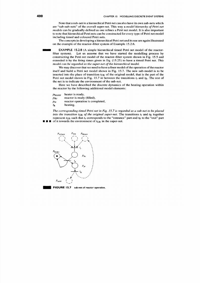
8/17/2019 Process Modelling and Model Analysis-Hangos-Cameron
http://slidepdf.com/reader/full/process-modelling-and-model-analysis-hangos-cameron 417/560
400 CHAPTER 15 MODELLING DISCRETE EVENT SYSTEMS
Note that a sub-net in
a
hierarchical Petri net can also have its own sub-nets w hich
are "sub-sub-nets" of the overall super-net. This way a
mode l hierarchy of Petri net
models can be gradually defined as one refines a Petri net mod el. It is also im portant
to note that hierarchical Petri nets can be constructed for every type of P etri net model
including timed and coloured Petri nets.
The conc epts in developing a hierarchical Petri net and its use are again illustrated
on the example of the reactor-filter system of Example 15.2.6.
I H H I EXAMPLE 15.2.8 (A simple hierarchical timed Petri net model of the reactor-
filter system). Let us assume that we have started the mod elling process by
constructing the Petri net model of the reactor-filter system shown in Fig. 15.5 and
extended it by the firing times given in Eq. (15.25) to have a timed Petri net. This
model can be
regarded
as the super-net of the hierarchical model
We may discover that we need to have a
finer
model of the operation of the reactor
itself and build a Petri net model shown in Fig. 15.7. The new sub-model is to be
inserted into the place of transition TGR of the original model, that is the part of the
Petri net model shown in Fig. 15.7 in between the transitions t^ and TR. The rest of
the net is to indicate the environment of the sub-net.
Here we have described the discrete dynamics of the heating operation within
the reactor by the following additional model elements:
theater heater is ready,
/7Rr reactor is ready (filled),
Pxx
reactor operation
is
completed,
T h heating.
The corresponding timed Petri
net in
Fig.
15.7 is
regarded
as a
sub-net
to be
placed
into the transition ^ G R of the original super-net. T h e transitions tx an d fR together
represent ^ G R such that t^ corresponds to the "entra nce" part an d fR to th e "exi t" p art
• I • of it
towards
th e
environment
of T G R in the
super-net.
^solvent ^raw PRem^i
I \ ( \ { \
^hea te r
t
^ s e m i
4
\
/ \
/ \
(
\
FIGURE 15.7 sub-
'r \
/
/
net
of reactor operation
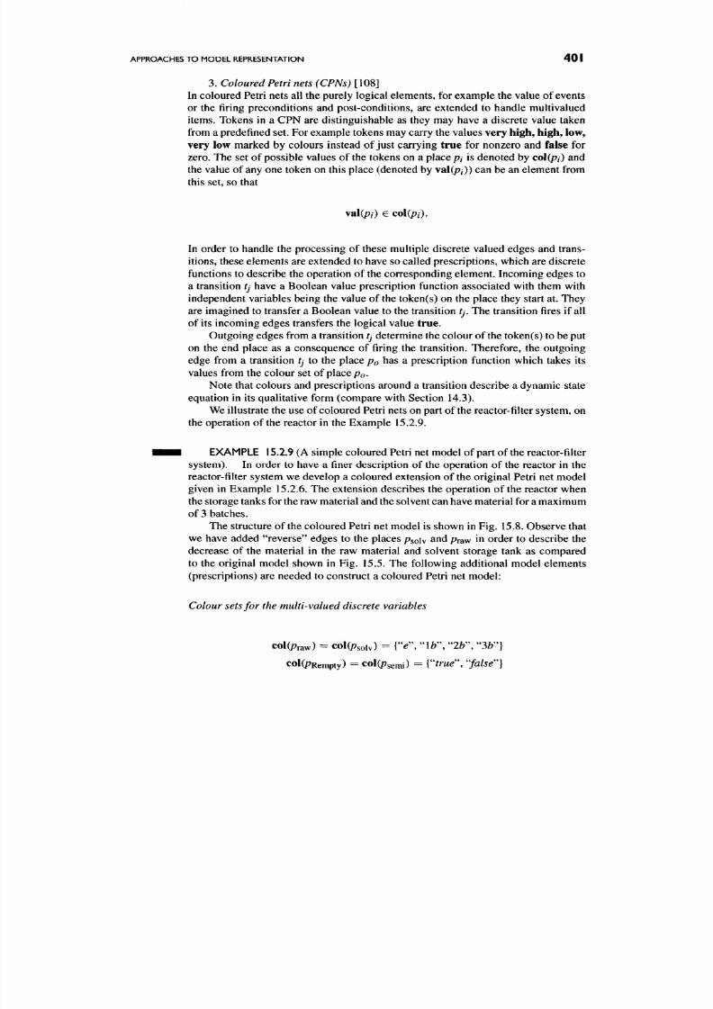
8/17/2019 Process Modelling and Model Analysis-Hangos-Cameron
http://slidepdf.com/reader/full/process-modelling-and-model-analysis-hangos-cameron 418/560
APPROACHES TO MODEL REPRESENTATION
401
3. Coloured Petri nets (CPNs) [108]
In coloured Petri nets all the purely logical elemen ts, for exam ple the value of events
or the firing preconditions and post-conditions, are extended to handle multivalued
items.
Tokens in a CPN are distinguishable as they may have a discrete value taken
from a predefined set. For example tokens may carry the values very high , high, low,
very low marked by colours instead of just carrying true for nonzero and false for
zero.
The set of possible values of the tokens on a place /?/ is denoted by col(pi) and
the value of any one token on this place (denoted by val(p/)) can be an element from
this set, so that
ysAipi) € colipi).
In order to handle the processing of these multiple discrete valued edges and trans
itions, these elements are extended to have so called prescriptions, which are discrete
functions to describe the operation of the corresponding element. Incoming edges to
a transition
tj
have a Boolean value prescription function associated with them with
independent variables being the value of the token(s) on the place they start at. They
are imagined to transfer a Boolean value to the transition tj . The transition fires if all
of its incoming edges transfers the logical value true.
Outgo ing edges from a transition tj determine the colour of the token(s) to be put
on the end place as a consequence of firing the transition. Therefore, the outgoing
edge from a transition tj to the place po has a prescription function which takes its
values from the colour set of place po.
Note that colours and prescriptions around a transition describe a dynamic state
equation in its qualitative form (compare with Section 14.3).
We illustrate the use of coloured Petri nets on part of the reactor-filter system, on
the operation of the reactor in the Example 15.2.9.
EXAMPLE 15.2.9 (A simple coloured Petri net model of part of the reactor-filter
system ). In order to have a finer description of the operation of the reactor in the
reactor-filter system w e develop a coloured extension of the original Petri net m odel
given in Example 15.2.6. The extension describes the operation of the reactor when
the storage tanks for the raw m aterial and the solvent can have material for
a
maximum
of
3
batches.
The structure of the coloured Petri net model is shown in Fig. 15.8. Observe that
we have added "reverse" edges to the places psoiv
^^^
Praw in order to describe the
decrease of the material in the raw material and solvent storage tank as compared
to the original model shown in Fig. 15.5. The following additional model elements
(prescriptions) are needed to construct a coloured Petri net model:
Colour sets for the multi-valued discrete variables
col(praw) = coKpsolv) = {'V, "Ifc", "2fc", "3fo"}
col(pRempty) = col(/7semi) =
{''true'\
Jalse'']
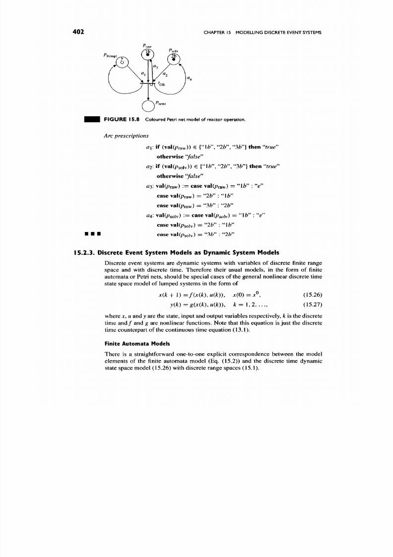
8/17/2019 Process Modelling and Model Analysis-Hangos-Cameron
http://slidepdf.com/reader/full/process-modelling-and-model-analysis-hangos-cameron 419/560
402
CHAPTER
15
MO DEL LING DISCRETE EVENT SYSTEMS
^ R e mpt
^solv
F I G U R E
15.8
Coloured Petri
net
model
of
reactor operation.
• • •
Arc prescriptions
ai : if (val(praw)) e rW\ "2fc", "3^"} then ''true''
otherwise
'Jalse''
ai : if (val(psolv)) € {"Ifc", "2fc", 3 7 } then ''true''
otherwise "false"
aa: val(/7raw) '-= case val(/7raw) = 1 ^ '- "^"
caseval(praw) = "2fo":"lfo"
case val(praw) = "3fo" : "2b"
a^ \
val(psolv) := case \2L\{psoiv) = 1 ^ : "^"
case val(psoiv) = " 2 ^ " : "\b"
case val(/7solv) =
" 3 ^ "
: "2b"
15.2.3. Discrete Event System Models
as
Dynamic System Models
Discrete event systems are dynamic systems with variables of discrete finite range
space and with discrete time. Therefore their usual models, in the form of finite
automata or Petri nets, should be special cases of the general nonlinear discrete time
state space model
of
lumped systems
in the
form
of
x{k + 1) =f{x(k ), u{k)), jc(0) = jc^,
y{k)=g{x{k),u{k)),
^ = 1,2, ... ,
(15.26)
(15.27)
where jc, u and y are the state, input and output variables respectively, k is the discrete
time and/ and g are nonlinear func tions. N ote that this equation is just the discrete
time counterpart of the continuous time equation (13.1).
Finite Automata Models
There
is a
straightforward one-to-one explicit correspondence between
the
model
elements of the finite automata model (Eq. (15.2)) and the discrete time dynamic
state space model (15.26) with discrete range spaces (15.1).

8/17/2019 Process Modelling and Model Analysis-Hangos-Cameron
http://slidepdf.com/reader/full/process-modelling-and-model-analysis-hangos-cameron 420/560
APPROACHES TO MODEL REPRESENTATION
403
State space mode l Au tom ata model Rem ark
x{k) e X
u(k)
€ U
fix(k).u(k))
x(k) e Q
u{k) e
E
(5
: e x E
Q
Set of possible states
Set of possible inputs
State transition function
Petri Net Models
In the case of Petri nets the correspondence between the model elements of the Petri
net model (Eq. (15.11 )) and the discrete time dynam ic state space model (15 .26) with
discrete range spaces as in Eq. (15.1) is not so simple and even not explicit as it was
the case for automata models.
It is important to realize that we need to use coloured Petri nets to make a one-
to-one correspondence between a discrete time dynamic state space model (15.26)
with discrete range sp aces as in Eq. (15.1) and a Petri net mod el to be able to describe
the value of the variables in the model. The following table summarizes the relation
between the model elements.
State space mo del Peri net mo del Rem ark
X , U
xik) e X
u(k) e U
f{x{k),u(k))
C = {co\(pi)\
I
/ = l , . . . , n }
/ x f ^ € COl(p/)
GpiVp^Ep)
Range spaces coded by colours
Places are for both states and inputs
Set of possible states and inputs
Encoded in the structure graph
(digraph and prescriptions)
15.2.4. Exception Handling in Discrete Event System Models
One of the most difficult p roblems in developing a discrete event model of a process
system is to ensure that the system m odel covers every possible sc enario. This usually
involves extending the model to include events for all possible faulty mo des. It should
encounter all exceptions which may o ccur during "norm al" operation.
The theoretical problem behind exception handling is the
completeness
of a
discrete model. A discrete event model is called complete if it is defined for every
possible state-input pair. Remember that finite automata models in Section 15.2.1
are not necessarily complete because the state transition function, 8, in Eq. (15.3) is
normally a partial function only, defined for some of the state-input symbol pairs.
From this understanding it is clear, at least theoretically, how one can m ake a discrete
event system model complete in order to handle all exceptions correctly: the state
transition function should be extended to make it complete. That is it should be
defined for every state-input symbol pair. In practice, however, extension of the set
of states as well as that of input symbols is usually necessary.
The following example shows how the consideration of every possible excep
tion (even in the simplest way ) makes the discrete event system model extremely
complicated.
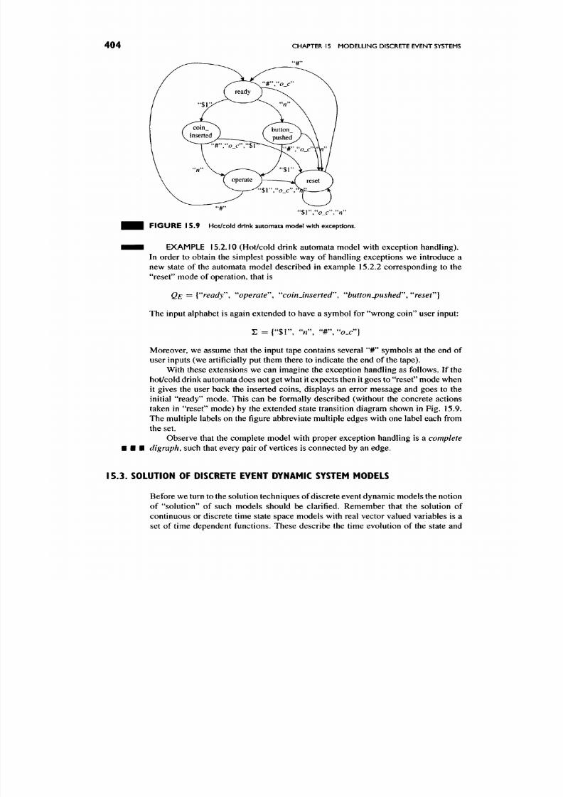
8/17/2019 Process Modelling and Model Analysis-Hangos-Cameron
http://slidepdf.com/reader/full/process-modelling-and-model-analysis-hangos-cameron 421/560
404 CHAPTER 15 MODELLING DISCRETE EVENT SYSTEMS
" $ r ' , " o _ c " , " n "
m FIG UR E 15.9 Hot/cold drink automata model wit h exceptions.
• • • EXAMPLE 15.2.10 (Hot/cold drink automata model with exception handling).
In order to obtain the simplest possible way of handling exceptions we introduce a
new state of the automata model described in example 15.2.2 corresponding to the
"reset" mode of operation, that is
Q^ — [''ready\ ''operate'', ''coinJnserted'\ ' 'button4>ushed'\ ''resef']
The input alphabet is again extended to have a symbol for "wrong coin" user input:
E =
{"$1",
"M ", "#" , "o_c"}
Moreover, we assume that the input tape contains several "#" symbols at the end of
user inputs (w e artificially put them there to indicate the end of the tap e).
With these extensions we can imagine the exception handling as follows. If the
hot/cold drink autom ata does not get what it expects then it goes to "reset" mode when
it gives the user back the inserted coins, displays an error message and goes to the
initial "ready" mode. This can be formally described (without the concrete actions
taken in "reset" mode) by the extended state transition diagram shown in Fig. 15.9.
The m ultiple labels on the figure abbreviate m ultiple edges with one label each from
the set.
Observe that the complete model with proper exception handling is a complete
• • •
digraph,
such that every pair of vertices is connected by an edge.
15.3. SOLUTION OF DISCRETE EVENT DYNAMIC SYSTEM MODELS
Before w e turn to the solution techniques of discrete event dynamic m odels the notion
of "solution" of such models should be clarified. Remember that the solution of
continuous or discrete time state space models with real vector valued variables is a
set of time dependent functions. These describe the time evolution of the state and
8/17/2019 Process Modelling and Model Analysis-Hangos-Cameron
http://slidepdf.com/reader/full/process-modelling-and-model-analysis-hangos-cameron 422/560
SOLUTION
OF
DISCRETE EVENT DYNAMIC SYSTEM MODELS 405
output variables over a given time interval assuming the time evolution of the input
variables and suitable initial conditions for the state and output variables are given.
In the case of discrete event system models, we need to specify the following
items for a well posed mathematical problem of determining its solution:
1.
A discrete event dynamic mathematical model—for example, a finite automata
or a Petri net model,
2. A time interval [fo, ^MI—with a given initial time t and final time tM over
which the solution will be computed,
3.
Initial conditions for the discrete valued state variables—in the initial time
instance tQ,
4.
A record for the input variables—containing a sequence of its discrete values
over the whole interval [fo, ^MI-
With these ingredients the solution of the discrete event model will be the time
evolution of the state and output variables, similar to the case of the state space models
with real vector valued variables. But now the time evolution will be given in terms
of a set of possible sequences of the discrete values for the state and output variables
in the form of
5[v](ro, tu) = {(v(ro), v{tx)..., v{tM)) I v(ro) =
VQ,
v{ti) e V, / = 1,2,..., M}
(15.28)
for the variable v, where VQ is its initial condition and V is its discrete range space as
in Eq. (15.1).
The solution of discrete event dynamic models is usually performed via discrete
event simulation. Here, the solution method is given in terms of a discrete algorithm
with executable steps instead of a numerical procedure or method. The combinatorial
nature of the solution of discrete event models will be seen on the examples of finite
automata and Petri net models described in the following two subsections.
15.3.1.
Solution of Finite Automata Models
If the discrete event system model of a process system is given in the form of a finite
automata according to Eq. (15.2) then the ingredients needed for the solution become
the following items:
1.
A discrete event dynamic model—in the form of
E q.
(15.2). It is important to
note that the set of discrete states of the automata Q is now constructed from
vectors
5^'^,
where theyth entry sj corresponds to the state variable Xj of the
system with range space Xj
)
I ; — n 1
N A: '
Q
=
[S^^
|/ =
0,
1,...,A ,
Sf
eX^
2. A time interval [to, tM]—with a given initial time to and final time tM over
which the solution will be computed. In case of non-timed models only the
required number of steps, M, is specified.
3.
Initial conditions for the discrete valued state variables—a concrete Go ^ Ql-
4.
A record for the input variables—which is now the content of the input tape.
In case of vector valued input variable the elements of the finite alphabet E are

8/17/2019 Process Modelling and Model Analysis-Hangos-Cameron
http://slidepdf.com/reader/full/process-modelling-and-model-analysis-hangos-cameron 423/560
406 CHAPTER 15 MODELLING DISCRETE EVENT SYSTEMS
again vectors E ^ '\ where the 7th entry E . correspond s to the input variable
Uj of the system with range space
U j
E = { E ( ' > | / = 0 , l , . . . , L , i : f
6(7 ;} .
Thereafter, the solution is generated in the following
conceptual algorithmic
steps:
A1 Take the given initial state Qo as the current state of the automata and set the
reading head of the input tape to the start of the tape. Put the initial state at
the head of the state sequence (or list) forming the so lution of the mod el.
A2 Test if there is any unfinished solution sequen ce. If there is not then STOP.
A3 Apply the state transition function 8 to the current (S^\ E^^) pair to get the
next state 5^"^^^ and increase the time. Check if the final time tM is not over.
If
so,
then STOP
• If this is unique then append the new state to the already generated state
sequence.
• If 5 "*~ ^ is not unique then form two identical state sequences for the set
of solutions to be continued.
• If a final state is reached S^^^^ e QF then close the solution sequence
by appending 5^+*^ to it and GO TO step A2.
• If the state transition function is not applicable to the current
{S^\
E^^)
pair then close the solution sequence and GO TO step A2.
A4 Set the state 5^"^^^ as the current state, move the reading head accordingly
and G O TO step A3.
The algorithm above is illustrated on the example of the reactor-filter system
introduced in Example 15.2.1 using its finite automata m odel given in 15.2.3.
^ • B EXAMPLE 15.3.1 (Solution of the finite automata model of the reactor-filter
system developed in Example 15.2.3). Com pute the solution of the model until an
infinitely large final time tM ^ith the following initial condition:
Qo == 'Jeeem
that
is,
all equipment is ready and with the content of the input tape:
(" r" ,"ni r ' ,#) , (15.29)
which corresponds to the case when a single batch is to be processed.
The state transition diagram shown in Fig. 15.3 will be the representation of the
model, we use for the solution.
Following the algorithm of solving finite automata models, we can easily
compute the following unique solution sequence:
g g g (' eeem»'^reen*'Jeren? »^eeem)» (1 5. 30 )
8/17/2019 Process Modelling and Model Analysis-Hangos-Cameron
http://slidepdf.com/reader/full/process-modelling-and-model-analysis-hangos-cameron 424/560
SOL UTION OF DISCRETE EVENT DYNAM IC SYSTEM MODELS 407
15.3.2.
Solution of Petri Net Models
In the case of discrete event process system models in the form of a Petri net the
ingredients needed for the solution are as follows:
1. a discrete event dynamic model—in the form of a Petri net structure. Here
the current state of the system is described by a marking with the places
corresponding to the entries in the state vector of the discrete event system.
2.
a time interval
[fo,
^M]—with
a given initial time fo and a final time
tM
over
which the solution will be computed. In case of untimed models only the
required number of
steps,
M, is specified.
3. initial conditions for the discrete valued state variables—which is now a
concrete initial marking.
4.
a record for the input variables—the input variables correspond to places in
the Petri net model with no inward directed edges. In order to imitate the
occurrence of the change in input signal sequence we associate a new place
acting as an external source. These source places put an appropriate token in
case of an input event. The external sources of tokens may be synchronized
by a special clock or by a timer, therefore we need a timed Petri net model in
case of multiple inputs for this purpose.
Thereafter the solution is generated by executing the Petri net model in the way
it was described in Section 15.2.2. The solution is obtained as set of finite or infinite
sequences of operations in the form of Eq. (15.20).
The solution of extended Petri net models such as timed, hierarchical and coloured
ones, proceeds much the same as that of the low level one, taking into account the
specialities of the models. The following changes should be made when computing
the solution of an extended Petri net model:
1. Timed Petri net models
Intermediate states (markings) should be introduced to describe the state of
the net during the firing times of a transient tj. Such an intermediate state can
be described by a marking /x^^ where the places of the pre-condition of the
transition loose their tokens, but places in the post-condition do not receive
any token.
2.
Coloured Petri net models
The firing pre-condition of any of the transitions tj should be computed from
the prescriptions of the incoming edges (they are all Boolean-valued expres
sions). Similarly, the post-condition, that is the colour of the tokens put onto
the places adjacent to the outgoing edges, is computed from the prescriptions
of the outgoing edges.
The solution of a low level Petri net model is illustrated on the example of
the reactor-filter system introduced in Example 15.2.1 with its Petri net model of
Example 15.2.6.
• 1 ^
EXAMPLE 15.3.2 (Solution of the Petri net model of the Reactor-Filter Sys
tem developed in Example 15.2.6). Compute the solution of the model when all
equipment is ready for processing and two batches
are
present to be processed.
8/17/2019 Process Modelling and Model Analysis-Hangos-Cameron
http://slidepdf.com/reader/full/process-modelling-and-model-analysis-hangos-cameron 425/560
8/17/2019 Process Modelling and Model Analysis-Hangos-Cameron
http://slidepdf.com/reader/full/process-modelling-and-model-analysis-hangos-cameron 426/560
ANALYSIS OF DISCRETE EVENT SYSTEMS
409
3. Finiteness or cyclic behaviour
In some discrete event systems there can be cyclic processes without any
natural stop. This makes the system non-finite.
4. Conflict situations
Conflict situations are usually discrete states for which the next state is non-
unique. The potential future states are in conflict and the choice has to
be resolved. The presence of conflict situations indicates ambiguity in the
discrete event model.
The first step in the analysis is the generation of the state transition diagram
introduced in Section 15.2.1 for the discrete event system mod elled by finite automata.
Equivalently, the reachability graph of the discrete event system modelled by Petri
nets is needed for the analysis.
The state transition diagram of the discrete event system contains the states,
events and the state transition function. This explains the need for discrete event
simulation when constructing the state transition diagram of discrete event systems.
15.4.1. Controllability or Reachability
A discrete event system is called (state) controllable or reachable if we can always
find an appropriate input function to move the system from its given initial state
to a specified final state in finite time. This applies to every given initial state final
state pair.
Given the state transition diagram of the discrete event system one can easily
check if the system is reachable. If the state transition diagram seen as a directed
graph is in itself a strongly connected component then the underlying discrete event
system is reachable. Note that a directed graph is a strongly connected component in
itself if there is at least one directed path from any vertex to any other vertex.
This mean s that every vertex pair in a strongly connected com ponen t is connected
by at least one directed path. The labels on the path form the input sequence moving
the system from the initial state vertex to the final one.
15.4.2. Deadlocks and Finiteness
Deadloc k is a state of the discrete event system from which any event, either external
or internal, cannot move the system out of it.
Cyclic behaviour is a set of states which occurs spontaneously and from which
any external event canno t move the system o ut of it. The presence of cyclic behaviour
causes the system to be non-finite in the sense that it "never stops".
Both deadlock and cyclic behaviour present in the discrete event system can be
analyzed based on its state transition d iagram. If
we
view the state transition diagram
as a weighted or labelled directed graph, then
• deadlock states can be detected as vertices with no outward directed edge,
• cyclic behaviour can be detected by finding a set of strongly connec ted state
vertices with no outward directed edge labelled by an external input event.

8/17/2019 Process Modelling and Model Analysis-Hangos-Cameron
http://slidepdf.com/reader/full/process-modelling-and-model-analysis-hangos-cameron 427/560
410 CHAPTER 15 MODELLI NG DISCRETE EVENT SYSTEMS
15.4.3. Conflict Situations
If the next discrete state of a given state with a given event is not unique then a conflict
situation arises:
the
next possible states
are in
conflict with each other.
In
Example
15.2.6
a
simple conflict situation
is
shown.
The
ambiguity
of
the next state
is
caused
by the improper definition of the state transition function when it has multiple values
for a given
(state, input symbol)
pair.
Conflict situations are easily detected on the state transition diagram seen as
a labelled directed graph. If a state vertex is found which has two or more outward
directed edges w ith the same label leading to different vertices then these state vertices
are in conflict with each other. This is a conflict situation in the discrete event system
model.
The analysis methods are illustrated on the example of the reactor-filter system.
^ • • i EXAMPLE 15.4.1 (T he an aly sis of the reactor-filter system of Example 15.2.1).
The state transition diagram
of
the discrete event model
of
the discrete reactor-filter
system is shown in Fig. 15.3.
The reactor-filter system is reachable because the state transition graph in Fig.
15.3 is a strongly connected component in itself. The input sequen ce "(r, nil)" moves
the system from state 5eeem back to itself.
There is no deadlock or cyclic behaviour present in the reactor-filter system
because there is at least one edge labelled by an external input event starting from
every state vertex.
The state transition diagram in Fig. 15.3 depicts the situation when the natural
conflict situation present
in
the reactor-filter system w ith
two
filters working
in
parallel
has been resolved using priorities:
if
the
next batch
of
the
raw material
is
present then
choosQ filterl dsefilter2.
This is seen in the labels of the outward directed edges of
• • • state 5reen- With these labels the discrete event system does not contain any conflicts.
15.5. SUMMARY
This chapter deals with discrete event systems from the viewpoint of process mod
elling
and
model analysis. This type of model
is
used when external
or
internal events
have a major impact on the behaviour of the process system and modelling focuses
on
the
sequential and/or parallel events taking place.
Based on the characteristic issues and main application areas of discrete event
process models the most important model representation methods, namely finite
automata and Petri net models are discussed. Following this, the solution of discrete
event process models via simu lation and the methods for analysis of their behavioural
properties, such as reachability, finiteness, deadlock s and conflict situation have been
described.
15.6. FURTHER READING
The
sources
of the literature on the field of discrete event systems and their application
in process systems engineering are to be found in books and papers and also on the
8/17/2019 Process Modelling and Model Analysis-Hangos-Cameron
http://slidepdf.com/reader/full/process-modelling-and-model-analysis-hangos-cameron 428/560
FURTHER READIN G
41 I
Web. The following list contains the most important information sources relevant to
the field:
• Journals
-
Com puters and Chemical Engineering
- AIC hE Journal
• Conferences
- ESCA PE Conferences
- IFAC Symposia "On -line fault detection and supervision in the chemical
process industries"
- International Conferences "A pplication and Theory of Petri N ets", where
the Proceedings are available as volumes in Lecture Notes in Computer
Science by Springer Verlag,
•
Web
-
Link 0ping University Division of Autom atic Con trol
hom epage: h t t p : / / w w w . c o n t r o l . i s y . l i u . s e
Becau se of the novelty of the field, the results on modelling discre te event process
systems can mainly be found in journal and conference papers, as well as research
reports. Some review papers can also be found from the field of systems and control
theory, such as [109,110].
The relevant papers can be most easily recognized based on the characteristic
application areas: batch process scheduling and process fault detection and isolation.
Here we mention only some of them classified according to the technique they use.
•
Finite automata techniques
A fault detection and isolation method based on the observation of events
applying finite automata for describing discrete event systems is presented
in [HI ] .
A framework is presented for synthesizing logic feedback controllers for
event-driven operations, such as startup and shutdown operations, emergency
procedures and alarm handling in
[112].
•
Discrete event simulation techniques
An autonomous decentralized scheduling system based on discrete-event
simulation is found in [113].
Short-term batch plant scheduling has been performed using a combina
tion of discrete-event simulation and genetic algorithms in
[114].
•
Grafcet description
A planning framework has been developed and applied for automating the
synthesis of operating procedures for batch process plants using
Grafcet,
a
discrete event modelling concept in [115] and [116].
•
Petri net approaches
A flexible, efficient and user-friendly system for HAZOP analysis of batch
process ing plant has been reported in [ 117] and [118] where the process model
is constructed as a combination of high-level Petri nets and cause and effect
digraphs.
An intelligent diagnostic system based on Petri nets is reported in
[119].
Petri nets have been used for modelling a supervisory control system of a
multipurpose batch plant [120].
8/17/2019 Process Modelling and Model Analysis-Hangos-Cameron
http://slidepdf.com/reader/full/process-modelling-and-model-analysis-hangos-cameron 429/560
412
CHAPTER
15
MODELLING DISCRETE EVENT SYSTEMS
15.7. REVIEW QUESTIONS
Q15.1. What are the key com ponents of a process system which contribute to the
discrete event behaviour? (Section 15.1)
Q15.2. Wh at are the key application areas in discrete event system modelling and
simulation? (Section 15.1)
Q15.3. What approaches are available in the literature to model a discrete event
dynamic system? (Section 15.2)
Q15.4.
Wh at are the elements of the formal description of a finite automata? H ow do
these elements appear in the state transition diagram of the autom ata? (Section 15.2.1)
Q15.5. Wh at are the elements of the formal description of a low level discrete Petri
net model? How are these elements visualized in the graphical description of the Petri
net? How do we describe the o peration or dynam ics of a Petri net in a formal and in
a graphical way? (Section 15.2.2)
Q15.6. Com pare the finite automata and the Petri net description of a discrete event
dynamic system. What is the relationship between the state transition diagram of the
automata and the reachability graph of the Petri net? (Sections 15.2.1 and 15.2.2)
Q15.7. Wh at kind of extended Petri nets are available for mod elling? How can we
use extended Petri nets for m odelling discrete event systems? (Section 15.2.2)
Q15.8. Wh ich dynamic properties of discrete event systems are the subject
of dynamic analysis? What is the definition and practical significance of these
properties? (Section 15.4)
Q15.9,
Wh at are the ingredients needed to perform the solution of a finite automata
model? What do you obtain as a result? How do we describe the solution method of
an automata model? (Section 15.3)
Q15.10. What are the ingredients needed to perform the solution of a Petri net model?
What do you obtain as a result? Describe the algorithm of solving a Petri net model.
(Section 15.3)
Q 1 5 . i l . Wh ich is the discrete event system m odel used for the analysis of dynam ic
properties? What is the first step of the analysis? Is the analysis of dynamic prop
erties of a discrete event system model computationally hard? Justify your answer.
(Section 15.4)
15.8. APPLICATION EXERCISES
A 15.1. Draw the state transition diagram of the reactor-filter system defined in
Example 15.2.1. Compare it to the state transition diagram shown in Fig. 15.3.
A15.2.
Develop a Petri net model for the problem of the hot/cold drink autom ata
described in Example 15.2.2. Extend it with processing times to get a timed Petri
net model. Show that the reachability graph of the model is the same as the finite
automata model shown in Fig. 15.2.
A15.3. Develop an extended version of the Petri net model of the emergency
shutdown procedure of example 15.2.7 to handle the following exceptions:
1. there is no inert gas available,

8/17/2019 Process Modelling and Model Analysis-Hangos-Cameron
http://slidepdf.com/reader/full/process-modelling-and-model-analysis-hangos-cameron 430/560
APPLICATION EXERCISES 41 3
2.
there is no cooling available,
3. the switch for turning off electricity from the equipm ent is out of service.
Draw the extended Petri net model starting from Fig. 15.6. How would you
proceed if you had to check the completeness of your model?
A
15.4.
Perform the simulation of the timed Petri net mod el of the emergency shut
down procedure of Example 15.2.7 shown in Fig. 15.6 starting with the initial
conditions (initial marking) shown on the figure up until a very large final time.
Draw the reachability graph of the model.
A 15.5. Perform the simulation of the timed Petri net mod el of the emergency shut
down procedure extended with exception handling in Application Exercise A15.3
starting with initial conditions (initial marking) which enable the firing of both
^cooling ^i d ffiii-neutr- Assu me that final time for the s imula tion is very larg e. Draw the
reachability graph of the model.
A15.6. Repeat the simulation of the Petri net model of the reactor-filter system
described in example 15.3.2 by adding finite firing (processing) times to the transitions
GR» ^Gfl ^i^d tQf2 such that
€ R
< 4 l < €f2- (15.34)
Is the solution uniqu e this time? C omp are the obtained solution(s) w ith the ones given
in Example 15.3.2.
A15.7. Unite the super-net and sub-net of the hierarchical Petri net of the rea cto r-
filter system described by Examp le 15.2.8, that is insert the sub-net shown in Fig. 15.7
into the super-net shown in Fig. 15.5. Give a suitable initial marking of the united
Petri net. Perform several steps in executing the united net and o bserve the operation
of the sub-net part.
A15.8.
Perform the simulation of the finite automata m odel of the hot/cold drink
automata extended with exception handling in Example 15.2.10 shown in Fig. 15.9.
Let the initial state be Qo = "ready" and the input tape contents be:
( a ) :
(b ) :
(c ) :
("$1","$1", "2" ,"#")
("2", "3" , "#")
("$ " ,"#" , "2" , "#")
A15.9.
Let us imagine a batch processing plant com posed of two reactors of equal
size, a large tank for cleaning solvent, another large tank for paint solvent, three
small vessels for pigments and three storage tanks for the prepared paints. The paint
of different colours is made in a single processing step in one of the reactors and
then fed to the appropriate paint storage tank. The reactors need to be cleaned after
processing if the next batch is a different colour. The processing and cleaning times
are given such that the cleaning takes much shorter time. The time needed for the
filling operation is negligible.
(a) Con struct a discrete event model of the plant.
(b) Perform simulations for different paint orders and under different conditions.
(c) Extend your model for the most common exceptions you may imagine.

8/17/2019 Process Modelling and Model Analysis-Hangos-Cameron
http://slidepdf.com/reader/full/process-modelling-and-model-analysis-hangos-cameron 431/560
414
CHAPTER 15 MODELLING DISCRETE EVENT SYSTEMS
A15.10. Analyse the behavioural properties of the timed Petri net model of a main
tenance shutdown procedure of Example 15.2.7 shown in Fig. 15.6. Try different
initial conditions (initial marking) including the one shown on the figure.
Can there be any conflict situations in the model? W hen?
How w ould you modify the model to avoid conflict situations? W hat would this
change mean in practice?
8/17/2019 Process Modelling and Model Analysis-Hangos-Cameron
http://slidepdf.com/reader/full/process-modelling-and-model-analysis-hangos-cameron 432/560
MODELLING HYBRID SYSTEMS
This chapter will discuss the modelling issues surrounding process systems which are
classified as either "dis crete -co ntinu ous " or "hyb rid" in nature. Some in the literature
also refers to these systems as "event driven". They are composed of elements which
contain discrete events at particular times or conditions combined with elements which
are basically continuous in behaviour. These represent an important class of process
problems.
The tools and techniques available for modelling and analysing discrete event
dynamic process systems were treated in Chapter 15. This chapter w ill cover the basic
ideas behind the modelling methodologies employed for hybrid systems with both
discrete and continuous parts, their analysis as well as the particular challenges for
their numerical solution, whether small or large-scale problems.
16.1. HYBRID SYSTEMS BASICS
16.1.1.
Characteristics and Issues
It can be convincingly argued that all process engineering systems are hybrid in nature.
We need to investigate what is meant by this statement. T here are several reasons why
systems consist of discrete behaviour either driven by events occurring in the system
or by external influences, whether planned or uncontrolled disturbances.
Figure 16.1 shows a typical process system emphasizing some of the key
components which contribute towards hybrid system behaviour.
415

8/17/2019 Process Modelling and Model Analysis-Hangos-Cameron
http://slidepdf.com/reader/full/process-modelling-and-model-analysis-hangos-cameron 433/560
416
CHAPTER 16 MODELLING HYBRID SYSTEMS
Operating Policies
Process System
Process Flowsheet
?
Physics/Chemistry
L
1
External disturbances
FIGURE 16 .1 Hybrid system characteristics.
The various compo nents can be considered to see where discrete event behaviour
might occur.
Process Flowsheet
The process flowsheet defines the processing units of the system and how they
are interconnected. Here we include the physical equipment and control system.
It is obvious that the equipment has various geometric characteristics which lead to
discrete behaviour.
These include:
• fixed capacity of tanks and vessels which can be filled, emptied or overflowed,
• decan ter systems which have specified baffle levels for overflow,
• comp ressor surge behaviour,
• changed use of flow paths depending on operating conditions, w hich may
switch feeds or energy streams,
• limiting conditions on operating or equipment parameters such as maxim um
pressure before a safety valve lifts or bursting disc operates,
• operating limits in the control elements such as control valves fully shut or
fully open or saturation of transmitter and controller outpu ts,
• "soft" constraints imposed by safety con siderations whereby process condi
tions are limited,
• operation of safety systems w hich limit process behaviour, switch protective
systems on or off and activate controlled or emergency shutdown systems.
All these, and mo re, impose discrete events on the underlying continuo us system
by virtue of the flowsheet design.

8/17/2019 Process Modelling and Model Analysis-Hangos-Cameron
http://slidepdf.com/reader/full/process-modelling-and-model-analysis-hangos-cameron 434/560
HYBRID SYSTEMS BASICS 417
Process Chemistry and Physics
This aspect, shown in
Fig.
16.1 represents the underlying chemistry and physics of the
process. Here, there are naturally occurring phenomena which contribute to discrete
behaviour. These characteristics can include:
• flow transitions between laminar, transitional and turbulent flow as represented
by flow models,
• chem ical reactions which accelerate rapidly or are "switched o n" by operating
conditions of temperature, pressure or composition,
• operational regimes such as boiling or non-boiling in steam-w ater or other
vapour-liquid systems,
• particle systems which are characterized by discrete items ,
• appearanc e and disappearan ce of vapour, liquid or solid phases due to chemical
activity and phase stability.
In many cases, such as metallurgical systems the phase behaviour is extremely
complex and leads to many discrete events which have to be handled within the
modelling of the system. Other processing operations such as those dealing with
particle enlargement or comminution reflect the basic discrete physical behaviour of
the physics.
Operational Policies
The operational policies imposed on the process can contribute to specific discrete
event behaviour of a system. In many cases, processes are run continuously or in batch
mode due in part to the underlying chemistry and the required production rate. Some
processes include continuous elements combined with batch stages. The principal
operational issues contributing to hybrid system behaviour include the following:
• Produc tion campaigns for multiple chemical products from a single continuo us
process, where product switching is done. Acetate ester production can be an
example of this operational policy.
• Regular switching of raw material feeds to the proc ess, an example being a
variety of crude oil feeds in a refinery.
• Regular product slate switches such as glass or fibreglass insulation thickness
changes to meet market demands.
• Chan ges in energy supply streams to processe s during start-up and energy
utilization on an integrated processing site.
These externally imposed changes or operating policies drive the underlying
continuo us sy stem through a series of discrete events which clearly reflect
the
imposed
operating policy.
External Disturbances
One major area giving rise to discrete events is the effect of uncon trolled d isturbances
on the process. The following illustrate typical examples of such events:
• thunder storms, rain, snow or atmospheric events,
• discrete chan ges in steam supply pressures from boiler systems.
8/17/2019 Process Modelling and Model Analysis-Hangos-Cameron
http://slidepdf.com/reader/full/process-modelling-and-model-analysis-hangos-cameron 435/560
418
CHAPTER
16
MODELLING HYBRID SYSTEMS
• power spikes in electrical supply systems,
• contamination of feeds to the process or specific feed characteristics such as
quality,
• market or seasonal dem ands for products.
The four fundamental sources of discrete event behaviour are usually represented
in some form in every process. W hether these characteristics are captured within the
modelling will depend on the modelling goal, the time frame considered and the
degree of fidelity required.
In this next section, we consider some typical application areas, where hybrid
models find use in describing the system.
16.1.2. Applications
Key application areas in hybrid system modelling and simulation include the
following:
batch processes for speciality chemicals, pharmaceuticals and paints,
continuous processes during start-up, shut-down and product changeover,
manufacturing systems where discrete items are processed on discrete
machines,
design of systems with units described by discrete variables such as staged
operations and binary variables (0,1) where they are present (1) or not
present (0).
A typical example of modelling for hybrid systems is given by the following
process w hich represents a forced circulation evaporator system w hich could be used
for concentrating sugar liquor or a fruit juice. Here, we are interested in the start-up
of
the
system. Figure 16.2 shows the flowsheet of
the
plant with a number of controls
for pressure, product concentration and level.
In considering the start-up of such a unit the steps of the procedure are shown in
Table 16.1.
This start-up sequence involves a number of discrete cha nges to flows, controller
settings and the start of pumps and other plant devices. The underlying process is
continuous but in this case the operational procedure imposes a series of discrete
events on the system.
Figure 16.3 shows the evaporator mass holdup during start-up, which clearly
shows the transient nature of the process as external changes take place.
The following section discusses the options available for representing hybrid
system behaviour. The approaches can be used for process systems and manufacturing
applications, for start-up, design and scheduling. The best representation depen ds on
the final application of the mo delling and the basic characteristics of the system being
modelled.

8/17/2019 Process Modelling and Model Analysis-Hangos-Cameron
http://slidepdf.com/reader/full/process-modelling-and-model-analysis-hangos-cameron 436/560
HYB RID SYSTEMS BASICS
419
vapour
P4.T3
cooling water
F200,
T200
^\A • condensate, F^
Condenser
F , .X , ,T ,
product
F I G U R E 16 .2 Forced circulation evaporator system.
TA BL E 16 .1 S ta r t -up procedure for forced c i rcu la t ion evapo ra tor
Ti m e (min ) Status or operat ion to be done
Time < 5
5 < Time < 7
7 < Time < 10
10 < Time < 20
20 < Time < 80
Time> 80
Time > 90
Time> 100
Time> 110
Time> 120
Feed flow = 0
Recirculation flow = 0
All controllers in m anual with 0 output
Set feed flow to fill shell in
2
min
All controllers in manual with 0 output
Recirculation flow = 0
Feed flow = 0
Recirculation flow = 0
All controllers in m anual with 0 output
Feed flow ramped to 5 kg/min
Recirculation flow ramped to 50 kg/min
Level controller set to automatic, setpoint =
1
m
Pressure controller set to automatic, setpoint =
50.5
kPa
Composition controller set to automatic, setpoint = 25%
Feed flow constant at
5
kg/min
Recirculation flow constant at 50 kg/min
Feed flow increased to
10
kg/min
Feed flow increased to
15
kg/min
Feed flow increased to
20
kg/min
Feed flow increased to 25 kg/min
Feed flow increased to
30
kg/min

8/17/2019 Process Modelling and Model Analysis-Hangos-Cameron
http://slidepdf.com/reader/full/process-modelling-and-model-analysis-hangos-cameron 437/560
420 CHAPTER 16 MO DEL LING HYBRID SYSTEMS
1200
100
200 300
time (minutes)
500
F I G U R E 16 .3 Evaporator mass changes during start-up.
16.2. APPROACHES TO MODEL REPRESENTATION
There are various but related approaches to describe a hybrid dynamic system with
both continuou s and discrete elements. From a system theoretic point of
view
a hybrid
system consists of three components:
• a discrete event dynamic system with discrete time and discrete valued
variables,
• a continuous system with continuou s variables,
• an interface between them.
Most approaches use combinatorial or finite techniques such as graphs or
automata extended by the capability to handle continuous elements. In this way,
the continuous elements are
imbedded
into a discrete dynamic structure.
Examples of these approaches outlined in this section are
1. extended finite automata models (hybrid automata) in Section 16.2.1,
2.
hybrid
Petri
nets
in Section 16.2.2,
3. differential-algebraic equations in Section
16.2.3.
The approaches are compared on the simple example of a reactor-filter sys
tem described in Chapter 15 in Example 15.2.1. This process system is regarded
as a hybrid system with all the equipment assumed to operate continuously form
ing the continuous part of the hybrid system. The steps of the operating procedures,
such as feeding, switching on/off equipments, etc. are discrete events acting on the
system.
8/17/2019 Process Modelling and Model Analysis-Hangos-Cameron
http://slidepdf.com/reader/full/process-modelling-and-model-analysis-hangos-cameron 438/560
APPROACHES TO MODEL REPRESENTATION 42 I
1 6 . 2 . 1 . Hybrid Automata
In the hybrid automata approach
1. the discrete event dynam ic system is described by a finite automata ac cording
to Section
15.2.1;
2. the continuous system is represented by its lumped nonlinear state space
model; and
3. the interface describe s how the events generated by the finite automata part
are transformed to act on the inputs and disturbances of the continuous part
and how the continuous part generates events to be fed to the finite automata.
Motivated by the above general parts and their functionality the general hybrid
automata model HA of hybrid systems consists of three com pon ents:
• a discrete event dynam ic system (DEDS ) described by finite automata
I>HA»
• a continu ous nonlinear system model described by a nonlinear state space
model
CHA»
• an interface between them described by special functions /HA-
Thus, the formal description of a hybrid automata model is a triple [121]:
W ^ = ( / > H A , C H A , / H A ) . (16.1)
The components of the above general hybrid automata model contain special
elements and properties to ensure their consistency and cooperation.
1. Discrete event dynamic system
The DEDS component of a hybrid automata model is the special case of the finite
automata model (15.2) in the form of
^ H A = (GHA» 5]HA» <5HA)-
QHA • The elements or coordinates in any state vector ^HA ^ QH A can be divided
into three different parts. First, there are elemen ts that correspond to actuator
or input variables. Second, there are elements related to different operat
ing regions due to geometric of physical structure of the continuous system.
Finally, there are elements corresponding to ordinary discrete states which are
not related to the continuous part.
E H A • The elements of the input alpha bet describe events in the DEDS model. The
set E H A is partitioned into three parts:
HA = 4Au4tu4A (16.2)
It consists of autonomous plant events ap 6 Ejj^^ generated from the contin
uous process by the event generator
y^ ^
in the interface. It also contains the
events E ^j^ , which occur spontaneo usly w ithout the influence of any modelled
(cr)
dynamics. Finally, there is the set of controllable input events E^j^.
^HA • is the usual state transition function.

8/17/2019 Process Modelling and Model Analysis-Hangos-Cameron
http://slidepdf.com/reader/full/process-modelling-and-model-analysis-hangos-cameron 439/560
422
CHAPTER
16
MODELLING HYBRID SYSTEMS
2. Continuous system
This part describes the continuous subsystem of the hybrid system using a special
version of the general nonlinear state space model equations (13.2):
Xp(t) =fp{xp{t), qp{t),
w(0, v( 0), (16.3)
^ (0 =
8p(xp(t), qp(t), M(0, V(0 ) ,
(16.4)
Zp{t) = hp{xp{t), u(t), v( 0) , (16.5)
where Xp(t) e TZ^ is the state vector of the continuous system, qp{t) e QHA is the
piecewise constant function from the
DEDS,
u{t) e Tl*^ is an external cons tant control
vector,
v{t)
€ 7?.^ is a continuous disturbance vector affecting the continuous states
and y{t) e IZ^ are the observable outputs.
The function
hp
gives the signal Zp{t)
e Zp c. 1Z^
which is the input to
yp
the
event generator in the interface.
Finally, to express jum ps in the continuous trajectory, a transition function 0p is
invoked
Xpif^) =
(f>p(Xp{t),
qp(t).
Op), (16.6)
which d etermines the starting values of the continuous state after an event
Op eUp,
3. Interface
This part determines the generation of a plant event Op e T,p from the continuous
system to the DEDS by the event generator
yp:Zp^
Ep . (16.7)
Events may occur for two reasons:
• if the system enters a region w ith a different behav iour and therefore is
described by a different model eq uation set from that previously used , or
• if there is a continuo us state jum p modelled by an internal event.
The above hybrid automata approach is illustrated on the example of the re ac tor-
filter system introduced already in Exam ple 15.2.1.
• • • EXAMPLE 16.2.1 (A hybrid automata model of the Hybrid Reactor-Filter
System introduced in Example 15.2.1)
The hybrid automata model of the reactor-filter system is constructed from the
finite automata model described in Example 15.2.3.
Discrete event dynamic system
First, observe that a discrete state vector q e CRF consists of four elements:
q =
[ST
Su
S2f Sinpf, (16.8)
• r, - if,
S2f e
{ r,
e],
^inp € {n,
m},
(16.9)
where Sr is the state of the reactor,
s\ f
and 52f are that
of filter a.nd
ilter2, and ^inp
is that of the reading head of the automata.

8/17/2019 Process Modelling and Model Analysis-Hangos-Cameron
http://slidepdf.com/reader/full/process-modelling-and-model-analysis-hangos-cameron 440/560
APPROACHES TO MODEL REPRESENTATION 423
The input alphabet or the events to the system are extended compared to the set
(15.5) to follow the decomposition in (16.2) in the following way:
Sp = {rr, rif, r2f}, (16.10)
Ev = {eT,eif,e2f,rso\w]. (16.11)
E/ =
{ r ,ml} ,
(16.12)
where rw, w = r, If, 2f and ^w, vv = r, If, 2f represent the occurrenc e of the
ready and empty status of the equipme nt, rsoiv is the availability of the solvent and r
is that of the raw material.
The state transition function is again an extension of Eqs. (15.6)-(15.10):
^RF(5'eeem, (r , ^solv)) = ^reen, (1 6. 13 )
^RF(^reen, /*r) = '^eem, (1 6. 1 4)
^RF('S'reen, ^r) = 5'eren, (1 6 .1 5)
^RF(5'eem, ^If) = ^eeem» (1 6. 16 )
^RF(5'eren, ^2f) = •^eeem. (1 6. 1 7)
Continuous system
The continuous system contains all three units: the reactor and the two filters.
Therefore, the continuous state vector Xp contains three parts:
Xp
= [Xr^if X2f] (16.18 )
where JCr, JCif an d jC2f are the state vecto rs of the reac tor and th e two filters respectively.
The fu nc tio n^ in Eq. (16.3) is composed of the corresponding state functions of the
reactor and the two filters acting on the corresponding state vector elements in (16.18).
These equations are active only if the equipment is working.
The working state of the equipme nt is represented by the following discrete state
vectors
qp
present in the argument list of 0p a n d ^ in Eqs. (16.6) and (16.3):
reactor: q^^^ = [e ee m ]^ , (16.19)
filterl:^^^^^==[reenf, (16.20)
filter2:^^l^> = [ reenf . (16.21)
The signal function hp in Eq. (16.5) can be defined on the continuo us state vector in
such a way that the event signal Zpit) takes four different values Zp\ Zp and Zp
if the reactor, filter 1 and filter is ready, and
Zp
if any of the processing steps are
taking place. For example,
Zpit) = z « if xr > x r ' \ x u = x t r ' . ^2f = ^ r " - (16.22)
Finally, the jump function 0p in Eq. (16.6) adjusts the continuous state vector to its
new initial state when an event in the discrete event dynamic system has taken place.

8/17/2019 Process Modelling and Model Analysis-Hangos-Cameron
http://slidepdf.com/reader/full/process-modelling-and-model-analysis-hangos-cameron 441/560
424
CHAPTER
16
MODELLING HYBRID SYSTEMS
For example the following jump is needed when the operation of the reactor starts:
V rt-^\ - Tv^^^P^y empty empty-iT
•^^v^
) — [- r -^ if -^2f J
= 0p(^p(O,
q^p\
(r, rsoiv)). (16.23)
Interface
Events in the continuous reactor-filter system may only occur if the system enters a
region with a different behaviour. The event is detected by the event signal ZpiO in
the continuous time system model. The event generator function yp maps the value
of the event signal into a plant event. The event generator function for the hybrid
reactor-filter system is as follows:
rr =
y{z^;^), (16.24)
rif = y{zj}^^), (16.25)
r2f =
y{z^^^^).
(16.26)
16.2.2.
Hybrid Systems Described by Petri Nets
Petri nets (see Section 15.2.2) are one of the most powerful and popular tools for
mod elling discrete event system s. In order to be able to handle the continuous part of
a hybrid system the original conc ept of Petri nets should be largely extended. Hybrid
systems can be described by Petri net in at least two different way s:
1. Timed
Coloured Petri
nets
[ 105]
The main idea of the approach is to convert the continuous part of the hybrid system
to a coloured Petri net by discretizing the time and the range space of the variables. In
this way the original nonlinear state space m odel of a lumped continuous time system
is converted to a set of constraint type qualitative differential equations having an
equivalent timed coloured Petri net representation. T he hybrid model is then conv erted
to a fully discrete model of an ap proximate discrete event system to the original hybrid
system.
2.
Hybrid
Petri
nets
[122]
Hybrid Petri nets use ordinary Petri nets for describing the discrete event dynamic
system.
The continuous system is modelled as a continuous Petri net. In this model, the
following extensions to the ordinary P etri net structure are defined:
• Infinitely many tokens can occur at all places . Real values of the Petri net state
described by the marking vector elements are approximated in such a way with
arbitrary precision.
• Instead of firing the transitions at certain time instants with zero duration there
is a continuous firing w ith a flow that may be externally generated by an input
signal and may also depend on the continuous marking vector.
8/17/2019 Process Modelling and Model Analysis-Hangos-Cameron
http://slidepdf.com/reader/full/process-modelling-and-model-analysis-hangos-cameron 442/560
APPROACHES TO MODEL REPRESENTATION 425
The continuous places and transitions are denoted by double circles and double lines.
In this way, a nonlinear state space model can be described using the continuous
Petri net.
The interface is modelled by special interface structure, such as switches, state
jum ps and boundary generators connecting discrete and continuous Petri net elements.
16.2.3.
Differential-Algebraic Systems
A natural representation of hybrid systems arises from the basic process engineering
modelling approach used in this book, namely in terms of conservation equations and
constitutive relations. However, in the case of hybrid systems there exists extra rela
tions which h elp to fully describe the system behaviour. Th ese relations are necessary
to define the events which o ccur in the system and the cond itions that apply after the
switching. As such, the overall description in terms of equations has an equivalent
representation in the form of a state transition graph. This con cept w as introduced in
Section 15.2.1.
A description in mathematical terms for a hybrid system consists of:
• The state equations which can be in various forms includ ing:
- ordinary differential equations (OD E),
- differential-algebraic equations (DAE) from lumped parameter mo dels,
- partial differential and ordinary differential-algebraic equations (POD AE)
from distributed system modelling,
- partial and integro differential-algebraic equations (PIODAE), arising
from the use of population balances within the model, such as those for
granulation dynamics,
• the cond itions under which the state switching occurs. These are typically in
the form of logical event statements containing boolean operators. They are
often encoded as I F . . . T H E N .. . E L S E .. . statements in the programming
language being used.
• The state of the system after the transition or switch has been ma de. Th is
allows the system solution to proceed.
The following sections set out in more precise terms these modelling elements
for hybrid systems. Following this, an example is given which illustrates the use of
these elements.
State Equations
The state equations are needed for each of the possible states in the state transition
graph for the process. If we assum e that there are n discrete states
[Ylu]^ / = , . . . , n)
in which the system exists, then we can write the dynamic state equations for each
state / as
fiixi,
Xi,
u,
rf, 0 = 0,
V
/ = 1 ,. . . , n, (16.27)
where
JC/
denotes the vector of states applicable to
J^u]
^ i th
u
and
d
denoting the sys
tem inputs and disturbances . These equations can also include the nonlinear algebraic
constraints associated with the DAE system.
8/17/2019 Process Modelling and Model Analysis-Hangos-Cameron
http://slidepdf.com/reader/full/process-modelling-and-model-analysis-hangos-cameron 443/560
426
CHAPTER
16
MODELLING HYBRID SYSTEMS
If
the
system state equations are either in the form of POD AEs or POID AEs then
the equations become:
fi(xi,
Xj,
x/,., ^/, ,
M,
^, r, 0 = 0,
V
/ = 1 ,. . ., n, (16.28)
where JC/ ,
jc,,.
represent the first and second derivatives of the states with respect to
the spatial variable
r.
Even though each state is represented by one of the n equations, it is clear that
in most process systems only a small set of equations change across the transition.
Hen ce, the actual total number of equations is often not greatly enlarged .
Event Equations
The event equations describe the conditions under which a transition is made between
the discrete state
Y,[i]
^^^ IZ[/]
•
Th ese conditions take the general form of:
E^^^j^
= E {xi,
x,v, x,v„
u ,
z,
t )
, (16.29)
and can be logical or functional statements w hich involve time, the state vectors and/or
their derivatives at the discrete state
J^[iy
Hence, the event equations can be
• simple time events, where a transition occurs at a specified time, are given by
IF time = t{
THEN
action needed
ENDIF
• state events where time is not known in advance but the switching occurs as a
function of the states, as given by
IF state condition function
THEN
action needed
ENDIF
The actions w hich occur in the system can be categorized into the following types:
•
Vector ield switching
wh ere the equation set changes in terms of equations and
variables. Typical exam ples are in the area of phase transitions like non-bo iling
to boiling regimes.
• State jumps where the underlying m odel does not change but the values of some
of the new states Xj in ^ ^ j do. Situations such as an instantaneous or almost
instantaneous addition of mass or energy to the system or implementation of
gain scheduling control can produce this form of switching.
• Task
descriptions,
where processing can take various forms such as
- serial tasks:
taskl -^
task -> • ->
taskN -^ end tasks
- parallel tasks: -> taskX -^ taskl -> • • • -^ taskN -> end tasks
->
tasklP -^ tasklP
-> • • • ^ -
taskMP
- ^
end tasks
- iterative tasks :-> taskl ->
task\
-> • • • -> taskl -> end tasks
8/17/2019 Process Modelling and Model Analysis-Hangos-Cameron
http://slidepdf.com/reader/full/process-modelling-and-model-analysis-hangos-cameron 444/560
APPROACHES TO MODEL REPRESENTATION 427
Transition Functions
These functions help relate the past states to the new states thus providing a unique
starting point for the solution to continue. They are typically of the form:
T^'^-^Hxi, Xj,
r,
M,
0
=
0. (16.30)
Hen ce, after a jump transition affecting a mass holdup JC[ in which an amount K of
component [1] is added to the system, the transition function could be:
xf^ =x]^^-hK, (16.31)
The proce dure of representing the system in these fundamental forms can also be
applied to each of the subsystem s within an overall system. He nce, large problems can
be decomposed into coupled subsystems and similar descriptions applied at the lower
levels. The overall behaviour is a summed total of all the individual contributions.
DAE Index Issues
Another important aspect of hybrid systems expressed as DAEs is the concept of
changing index of the equation set. The index can change significantly because of
the imposition of new constraints on the system differential (continuous) variables
imposed by the event equations and the transition functions. DAE systems that were
originally index-1 can take on higher index properties as switching occurs and the
reverse can occur. The example problem has this behaviour.
• • • EXAMPLE 16.2.2 (The water cistern system ). Con sider the following simple
problem as an illustration of the key hybrid concepts.
The system in Fig. 16.4 represents a typical overflow design for a water cistern.
Water enters the outer tank at a rate m/ and drains out at rate mi. If the outlet flow
from tank 1 is less than the inlet flow then the water will overflow into the second
internal tank at rate
nit
• At this point the outer tank has a fixed liquid height of
/i.
If the
inner tank level continues to climb, then it too will reach a liquid height determined
by the inner tank wall. Liquid height continues to rise above height h, until the tank
overflows at height
H.
Hence, it can be seen that this system has a number of states
and transitions which determine the state transition graph. Other transitions occur.
Figure 16.5 shows the four principal states of the system (X][/]» ' = 1 , . . . , 4).
The following mathematical description gives the state equations, the event
equations and transitions when the event condition is violated.
Ai -—- = m/ — mi — nit, (16.32)
at
A2-^— = mt — m2 (16.33)
d^
with the conditions that define the states being:
State 1:
E^^^^\ hi <h,
E^^^^\ h2 < K
mt = 0.

8/17/2019 Process Modelling and Model Analysis-Hangos-Cameron
http://slidepdf.com/reader/full/process-modelling-and-model-analysis-hangos-cameron 445/560
428
CHAPTER 16 MODELLING HYBRID SYSTEMS
H
jm^
m.
t m ,
FIGURE 16 ,4 Wa ter cistern schematic.
State 2
State 3 State 4
FIGU RE 16 .5 Possible system states for the cistern.

8/17/2019 Process Modelling and Model Analysis-Hangos-Cameron
http://slidepdf.com/reader/full/process-modelling-and-model-analysis-hangos-cameron 446/560
APPROACHES TO MODEL REPRESENTATION
429
State 3:
State 4:
State 2:
£;<2-l), ntt > 0 ,
£<2.4),
h2<h,
hi =h.
£<3.1)^ m f < 0 ,
h2
—
h.
E^^'^\ hx
>
h,
£(^•2),
h2>h,
h\ = /i2.
The state transition graph is given in Fig. 16.6. If any of the conditions in a
particular state are violated, then the particular event equation switches the system
to a new state. For example, if in state 3 (XI[3]) th^ transfer flow rrit becomes zero,
then the event equation
E^^'^^
activates and the system moves to state 1 (Xl[i])- ^t is
clear that apart from state 1, all other states lead to DAEs of index-2 because of the
imposed algebraic conditions on the continuous (differential) variables.
The solution of the equation systems requires special solvers that can handle
the index-2 problem or further transformation to reduce the system to index-1 via
differentiation of the constraint equations du e to the transitions .
£(1 .2)
£(3.1)
£(2,4)
£(4,3)
F I G U R E
i
6. 6 State transition graph for water cistern model.
8/17/2019 Process Modelling and Model Analysis-Hangos-Cameron
http://slidepdf.com/reader/full/process-modelling-and-model-analysis-hangos-cameron 447/560

8/17/2019 Process Modelling and Model Analysis-Hangos-Cameron
http://slidepdf.com/reader/full/process-modelling-and-model-analysis-hangos-cameron 448/560
SOLUTION OF HYBRID SYSTEM MODELS 43 I
com putationally hard for all but the simplest of problem s, this method fully accoun ts
for the nonlinear dynamics.
16.4. SOLUTION OF HYBRID SYSTEM MODELS
16.4.1.
Differential-Algebraic Equation Systems
These systems are the most typical of dynamic problems in hybrid modelling. As
such the numerical solution methods need to specifically address the characteristics
of hybrid problems. Several approaches are available to address the problems, how
ever most numerical solution software for these problems remains tied to specific
simulation packages with little in the public domain that addresses the challenges.
Key Challenges
The key challenges in solving hybrid DAE systems are as follows:
• Efficient solution of small and large problem s, which might exploit structural
aspects like parallelism and sparsity in the equation system.
• Robu stness of solution such that a reliable solution is generated in reasonable
time.
• The ability to handle time events, where switching times are known in advance.
• The ability to handle state variable events, where the time of the event is not
known.
• The ability to detect state variable event occurrenc es.
• The ability to locate the time at which state variable events occur.
• The ability to restar t efficiently at the new state.
• The ability to handle situations where the number of variables/equations
changes for various states.
• The ability to handle higher index problems (typically index -2).
Differential Systems
The solution of pure differential systems has already been dealt with in Chapter 6.
There are numerous codes available to solve these problems. However, there are few
codes which routinely handle the ODE problem, where discontinuous behaviour is
present. This is even less so with DAE systems. Specialized numerical codes are
needed for such tasks and are normally part of a larger simulation environment such
as
Speedup, gPROM S
[125] or
Daesim Studio
[126]. Most, if not all, only deal with
index-1 DAE problems. There are several codes for higher index problems, which
are based on Runge-Kutta formulae including those by Hairer and Wanner [127],
Williams et al. [50]. Only the latter addresses large sparse hybrid DAE problems of
index-1 or-2.
Little exists for solution of hybrid partial-ordinary differential and algebraic equ a
tions or partial integro-differential and algebraic equation sy stems, w hich require a
choice of discretization m ethod for the partial differential equations u sing such tech
niques as finite difference, orthogonal collocation or finite elements. Some of these
techniques are given in Chapter 8. In the case of partial integro-differential equation s.

8/17/2019 Process Modelling and Model Analysis-Hangos-Cameron
http://slidepdf.com/reader/full/process-modelling-and-model-analysis-hangos-cameron 449/560
432
CHAPTER 16 MOD ELLING HYBRID SYSTEMS
decisions have to be made about hand ling the integral terms. For particulate systems,
Hounslow's technique [128] has found widespread application.
Event Detection
A key requirement for hybrid system solvers is the ability to detect when an event has
occurred which moves the process to a new node on the state transition graph. The
easiest event detection is the time event which is typically prespecified by the user in
an event list. The nu merical m ethod can be mad e to step directly to the specified event
time within the mac hine accuracy, activate the state transition, then resum e solution.
The m uch greater challenge is efficient state variable event detection where the
transition is determined by the event equations
E^^'J^
= E^J
(jc/, JC/,., jc/ . ,
M,
Z,
t ). Here
the time of event is not known but is implicit in the event equations. These equations
can be checked at each step of the integration routine to see w hether a change of sign
has occurred. If so, then a switching point has been passed in the current step of the
solver. This is seen in Fig. 16.7 which shows the behaviour of a number of event
equations over a solution step (f„, f/j+i).
In this case, there are two event functions which change sign. E^-^^ changes
(+ )
-^
(-) and
E^ ''>
changes (-) -> (+), with E^' J remaining (+). However the
time
ts i
at which E^-^^ changes sign occurs before event E^^' at time ts2' Hence, this
change must be handled first. In all cases of event detection over a solution step, there
must be a precedence ordering of all the event function sign changes with the first
located and then activated. Of course, this activation of the first event can then ch ange
the pattern displayed by subsequent event functions. Thus, the detection algorithm
must identify and sort all active events over the step.
(+)
(-)
E(J^k)
\
• • • . ^ s l
1
T^.
tn .-<
^
/
/
/
y
z'
/
/Eik, 1)
hi y^
•
~7^
y
1
^ . + 1
w
^
time
F I G U R E 16 .7 Event function behaviour over a solution step.
8/17/2019 Process Modelling and Model Analysis-Hangos-Cameron
http://slidepdf.com/reader/full/process-modelling-and-model-analysis-hangos-cameron 450/560
SOL UTION OF HYBRID SYSTEM MODELS 433
Even though in Fig. 16.7, the event functions are shown as continuou s functions,
it is normally not the case that much information is known about the event function
behaviour between discrete solution outputs. Simply what is known in most cases,
such as the use of linear multi-step methods, is a change of sign from
tn
to
tn^\
. In
some cases, the internal stage calculations can actually help detect the event function
change before the end of the current step.
Alternatively, information can be kept about the event functions E^^'J which
allows prediction of possible sign changes before the current step is taken. This
represents a "look ahead" strategy for event times. This can be useful in improving
the efficiency of the event detection.
Event Location
Having identified that an event, or several events may have oc curred in the last step,
it is necessary to locate within a prescribed tolerance the time of the first event. This
normally requires an interpolation routine applied iteratively until the event time is
located to a user set toleranc e. In many cases only a few iterations are needed to locate
the event time, depending on the quality of the interpolant.
Becau se event functions can consist of either state and/or algebraic variables, the
location algorithm must handle both cases.
After location of the event, it is necessary to ensure that the new state is activated
and the transition cond itions given by the function T ^ ^ imposed . This can be difficult
at times, since a number of issues could be important, including:
• chang e of index. From index-1 to index-2 or higher as well as the reverse
situation,
• chang e of numbers of equations and variables from one state to another in the
state transition graph.
Restart of Solution
There are several issues which must be addressed when restarting the solution after a
state transition. This depends direcdy on the type of solver being used.
Linear multi-step methods In the case of the LM M s, whether explicit or implicit
formulae, these techniques rely on past solution points to generate a high order rep
resentation of the solution. Unfortunately, once a state transition takes place, the past
information
is
invalid from the perspective of
the
polynom ial representing the solution.
Hence, L MM s typically revert to order 1 methods which are either Euler or backward
Euler methods depending on whether they are explicit or implicit. The LMMs then
gradually build up the order of the representation via the standard step/order change
mechanisms.
In order to handle highly discon tinuous problem s, it is possible to restart the solu
tion with a higher order Rung e-K utta formula which generates sufficient information
to then switch back to the LMM after a few steps. No generally available production
codes are available for this purpose.
Runge-Kutta methods
The advantages of Run ge-Ku tta methods for highly discon
tinuous problems is obvious from their use in LMMs for restart. The key advantage
is the maintenance of high order across a state transition. Being single step methods
8/17/2019 Process Modelling and Model Analysis-Hangos-Cameron
http://slidepdf.com/reader/full/process-modelling-and-model-analysis-hangos-cameron 451/560
434 CHAPTER 16 MODELLING HYBRID SYSTEMS
they use the last solution point only as the starting point for the numerical solution
over the current step. Hence, the main issue is related not to maintenance of order
but to a rapid step increase mechanism which quickly brings the steplength to the
appropriate level to maintain local error tolerance s.
High-Index Solvers
As was mentioned in Section 16.2.3, state transitions can often mean changes not
only in the size of the equation set but also its differential index. The example of
the water cistern system in Section 16.2.3 shows how index can change from 1 to 2
and back again. In these cases, high-index solvers can be used. However, there are
few high-index solvers available. Most reliable index-2 (or higher) solvers are based
on Runge-Kutta formulae. Programs such as RADAU5 [129] and ESDIRK provide
efficient solution of index-2 problems [5 0].
Linear mu ltistep methods such as the BDF can be made to solve index-2 problems
but usually at a significant cost in efficiency.
Transformations for DAE Systems of High Index
There are a number of modelling transformations which can be used to alleviate
high index DAE solution problems. In the DAEPACK by Barton [47] this problem
is handled by the introduction of dummy derivatives. Other techniques requiring the
differentiation of subsets of the algebraic system can also be used [40 ].
16.5.
SUMMARY
This chapter has developed the background theory and applications of hybrid system
mo dels. It can be said that all real processes are essentially hybrid in nature, only that
in many situations we pretend that they are continuous for reasons of simplicity and
solvability.
The chapter has investigated the current major representation of these systems
highlighting the characteristics of hybrid automata, Petri nets, and differential-
algebraic systems.
These systems continue to be a major challenge for researchers and application
software experts.
There is much to be done in this area from a systems perspective, in order to
provide robust and transparent modelling systems for the process industries.
16.6.
FURTHER READING
The literature on modelling of hybrid process systems is mainly centered around the
particular tools and technique s applied for solving a particular problem . Unfortunately
little is known and almost nothing has been published on the comparison of the
different available approa ches.
Because of the scattered and rapidly developing nature of the
field
further reading
is recomm ended mainly for recent journ al and conference papers. There
are,
however,
some review papers mainly from the field of systems and control theory, such as
8/17/2019 Process Modelling and Model Analysis-Hangos-Cameron
http://slidepdf.com/reader/full/process-modelling-and-model-analysis-hangos-cameron 452/560
REVIEW QUESTIONS 435
[109,110]. We only cite some of the most characteristic application papers from
the field of process systems engineering arranged in groups driven by the technique
they use.
• The
discrete event system m odelling approach
applied to process system s with
hybrid nature has been presented by Preisig [130].
• An optimization problem, the derivation of an optimal periodic schedule for
general multipurpose plants comprising batch, semi-batch and continuous
operations resulted in a mixed integer nonlinear programming (MINLP) prob
lem in [ 131]. The basis of the hybrid system model is the general resource-task
network (RTN) coupled with a continuous representation of time.
A similar problem, on-line scheduling of a multiproduct polymer batch
plant has been solved in [132]. Instead of solving the resultant large, non-
convex MINLP problem by conventional optimization packages, they applied
genetic algorithms to generate the schedules.
• The
simulation approach
is used in [133] for complex operability analysis of
dynamic process systems under the influence of exceptional events, such as
failures and sudden changes.
16.7.
REVIEW QUESTIONS
Q16.1. Wh at are the key compon ents of a process sy stem which contribute to the
hybrid behaviour? (Section 16.1)
Q16.2. Wh at are the key application areas in hybrid system mo delling and simula
tion? (Section 16.1)
Q16.3. What are the three components in a hybrid system? Wh at approaches are
available in the literature to model the discrete event com ponen t? (Section 16.2)
Q16.4,
What are the elements of the formal description of a hybrid finite automata?
How do these elements appear in the state transition diagram of the automata?
(Section 16.2.1)
Q16.5. Give the formal description of the three com ponen ts of a hybrid autom ata
model: the discrete event dynamic system, the continuous system and the interface.
What are the extensions needed in the discrete event component and continuous
component to fit them into the hybrid automata framework? (Section 16.2.1)
Q16.6. W hat kind of extended Petri nets are available for modelling hybrid systems?
How can we use Petri nets for modelling hybrid systems? (Section 16.2.2)
Q16.7. Wh ich dynamic properties of hybrid systems are subject of dynam ic analysis?
Wh at is the definition and practical significance of these properties? (Section 16.3)
Q16.8.
Wh ich is the hybrid system mod el used for the analysis of dynamic proper
ties? What is the first step of the analysis? Is the analysis of dynamic properties of a
hybrid model computationally hard? Justify your answer. (Section 16.3)
Q16.9. What are the key issues in numerical solution of hybrid DAE models?
(Section 16.4)

8/17/2019 Process Modelling and Model Analysis-Hangos-Cameron
http://slidepdf.com/reader/full/process-modelling-and-model-analysis-hangos-cameron 453/560
436 CHAPTER 16 MODELLING HYBRID SYSTEMS
16.8. APPLICATION EXERCISES
A16.1. Draw
the
extended state transition diagram of
the
reactor-fiher system defined
in Example 16.2.1 as the discrete event part of the hybrid model. Compare it to the
state transition diagram shown in Fig. 15.3.
A16.2. Consider the state transition graph of the water cistern model shown in
Fig. 16.6. Is the underlying hybrid system reachable? Has it got any deadlocks or
conflict situation?
A
16.3.
Construct the hybrid automata model of the water cistern system in
Section 16.2.3.
A16.4.
Construct the hybrid Petri net model of the water cistern system in
Section 16.2.3.
8/17/2019 Process Modelling and Model Analysis-Hangos-Cameron
http://slidepdf.com/reader/full/process-modelling-and-model-analysis-hangos-cameron 454/560
MODELLING APPLICATIONS
IN
PROCESS SYSTEMS
In this chapter, we outline some modelling applications on a variety of process
systems. The purpose of these applications is to show the general methodologies
discussed in earlier chap ters. Other important issues to do w ith plant data acq uisition
and the application of numerical techniques for solution are highlighted. Also the
need to revise the assumptions underlying the model and hence the mathematical
model itself is an important issue, where there are significant discrepancies between
the model predictions and the plant behaviour.
The exam ples have been chosen to illustrate a wide variety of process application
areas and the intended use of the models in an industrial or research environment.
The m odels make no claim to being the most accurate or comprehensive, but simply
illustrate various approaches to the problems being addressed.
The modelling examples addressed in this chapter include:
• high temperature copper converter dynamics (minerals processing),
• phenol destruction in waste water using a photoch emical reaction process
(environmental engineering),
• dynam ics of drum granulators and granulation c ircuits (particulate
processing),
• prefermentation in wastewater treatment (wastewater enginee ring),
• dynam ics of an industrial depropan izer (petrochem ical proc essing).
437

8/17/2019 Process Modelling and Model Analysis-Hangos-Cameron
http://slidepdf.com/reader/full/process-modelling-and-model-analysis-hangos-cameron 455/560
438
CHAPTE R 17 MO DEL LING APPL ICATIONS IN PROCESS SYSTEMS
17.1. COPPER CONVERTER DYNAMICS
This application concerns the modelling for dynamic analysis and optimal control of
a 32 0 tonne reactor for liquid copper processing . This is a fed batch reactor w ith both
continuous and discrete addition and extraction of materials.
17.1.1. Process Description
In the industrial process for making copper metal from chalcopyrite ores, copper
concentrate being about 5-10% copper with the rest being sulphides, iron and other
minerals is reacted in a high intensity smelter with oxygen. This produces a matte
copper of around 50% copper with substantial amounts of sulphur and iron. These
impurities must be removed so that liquid copper can be cast into anode plates for
electro-refining. To do this, a high temperature Pierc e-Sm ith co nverter is used to give
95.5% copper produ ct. Figure 17.1 shows a typical industrial converter of around 350
tonnes capacity. The converter is 4.5 m diameter and 15 m in length.
The operation of such a converter requires the discrete addition of matte copper
from 25 ton ladles as well as many discrete additions of silica flux, solid re-work
copper, anod e skim and other m aterials over the time of the complete cycle. Constant
sparging of air through injection tuyeres located 300 mm below the bath surface
promotes the oxidation of sulphur compounds, the formation of slag phases and
finally liquid copper. Slag, which contains unwanted iron compounds is periodically
drained off by "rolling out" the reactor. The operation is typically divided into two
distinct periods, known as the "slag making phase" and the "copper making phase".
FIGURE 17 .1 Depiction of rolled-out converter pouring to a pot.

8/17/2019 Process Modelling and Model Analysis-Hangos-Cameron
http://slidepdf.com/reader/full/process-modelling-and-model-analysis-hangos-cameron 456/560
COPPER CONVERTER DYNAMICS
439
F I G U R E 1 7 . 2 Scenario
FIGURE 17 .3 Scenar io
The process is characterised by intense exothermic chemical reactions, high radiative
heat transfer and complex phase behaviour with up to nine phases present.
There are three key operational periods for the converter:
1. The idle period, which is between batches, where cooling and possible
solidification of residual co ntents occ urs. This could be 45 min in du ration.
2. The slag making period, wh ere sulphur is oxidized and released as SO2 and
iron is oxidized into a silica saturated s lag. This p eriod lasts about 90 min
with the bath being mainly CU2S. This is termed "white metal".
3. The copper making period, where liquid copper begins to form as CU2S is
oxidised by air injection leaving a "blister" copper of around
1.5-1.9
wt %
sulphur and a significant amount of oxygen. This period is about 150 min.
The graphics in Figs. 17.2-17.4 show the three principal scenarios for radiation
calculations . Scenario 1 relates to an empty converter during the idle period. Scen
ario 2 is when the converter is charged and "rolled in", whilst Scenario 3 covers the
case wh ere the converter is charged but "rolled out" and w here losses to the hood are
important.
Modelling Goal
To predict the dynamic behaviour of the system as a result of a specified event
sequence.
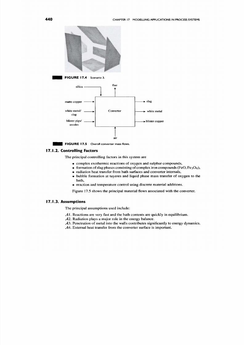
8/17/2019 Process Modelling and Model Analysis-Hangos-Cameron
http://slidepdf.com/reader/full/process-modelling-and-model-analysis-hangos-cameron 457/560
440 CHAPTER 17 MO DEL LING APPLICATIONS IN PROCESS SYSTEMS
F I G U R E 1 7 . 4 S c en ar io s.
silica
matte copper
white metal/
slag
blister pigs/
anodes
flue
•
•
^
i
'
k
Converter
i k
•
•
> slag
white metal
> blister copper
H J H F I G U R E 1 7 . 5 Ove ra ll c on ve rt er ma ss flo ws .
17.1.2. Controlling Factors
The principal con trolling factors in this system are
• complex exothermic reactions of oxygen and sulphur com poun ds,
• formation of slag phases consisting of complex iron com pound s (FeO, Fe304),
• radiation heat transfer from bath surfaces and converter internals,
• bubble formation at tuyeres and liquid phase mass transfer of oxygen to the
bath,
• reaction and temp erature control using discrete material additions.
Figure 17.5 shows the principal m aterial flows associated with the converter.
17.1.3. Assumptions
The principal assumptions used include:
Al. Reactions are very fast and the bath contents are quickly in equilibrium.
A2.
Radiation plays a major role in the energy balanc e.
A3,
Penetration of metal into the walls contributes significantly to energy dynam ics.
A4.
External heat transfer from the converter surface is important.
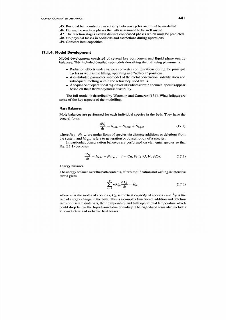
8/17/2019 Process Modelling and Model Analysis-Hangos-Cameron
http://slidepdf.com/reader/full/process-modelling-and-model-analysis-hangos-cameron 458/560
COPPER CONVERTER DYNAMICS
441
.45. Residual bath contents can solidify between cycles and must be modelled.
A6. During the reaction phases the bath is assumed to be well mixed.
Al.
The reaction stages exhibit distinct conden sed phases which must be predicted.
^ 8 . No physical losses in additions and extractions during operations.
v49. Constant heat capacities.
I 7 J A Model Development
Model development consisted of several key component and liquid phase energy
balances. This included detailed submodels describing the following phenomena:
• Radiation effects under various converter configurations d uring the principal
cycles as well as the filling, operating and "roll-out" positions.
• A distributed param eter submodel of the metal penetration, solidification and
subsequent melting within the refractory lined walls.
• A sequence of operational regions exists where certain chemical species appear
based on their thermodynamic feasibility.
The full model is described by Waterson and Cameron [134]. What follows are
some of the key aspects of the modelling.
Mass Balances
Mole balances are performed for each individual species in the bath. They have the
general form:
^ = A ^ M n - A ^ / , o u t + i V / , g e n , ( 1 7 . 1 )
where A^/jn^ M,out are molar flows of species via discrete additions or deletions from
the system and A(/,gen refers to generation or consumption of a species.
In particular, conservation balances are performed on elemental species so that
Eq. (17.1) becomes
^ = A^ i„ - Ni^^^t, i = Cu, Fe, S, O, N, SiOa. (17.2)
at
Energy Balance
The energy balance over the bath con tents, after simplification and writing in intensive
terms gives
Jl^'i^Pi^ = ^B.
(17.3)
where «/ is the moles of species /, C^. is the heat capacity of species / and
EB
is the
rate of energy ch ange in the bath. This is a com plex function of addition and d eletion
rates of discrete materials, their temperature and bath operational temperature which
could drop below the liquidus-solidus boundary. The right-hand term also includes
all conductive and radiative heat losses.

8/17/2019 Process Modelling and Model Analysis-Hangos-Cameron
http://slidepdf.com/reader/full/process-modelling-and-model-analysis-hangos-cameron 459/560
442 CHAPTER 17 MODELLING APPLICATIONS IN PROCESS SYSTEMS
Radiative Energy Losses
Radiation heat transfer was computed using detailed estimates from a Monte-Carlo
ray-tracing algorithm to evaluate radiative heat exchange amo ngst the vessel interior
and the converter mouth. The model incorporates gas radiation from SO2 fractions
within the enclosures, and also co nsiders m irror-like reflections from the bath surface.
The radiation enclosures were selected based on the geometric scenarios previously
mentioned.
The model accounts for external radiation from the shell, the ends and the
converter mouth.
Conductive Energy Losses
Unsteady -state heat conduction is used to describe heat losses from the internal w alls
of the converter:
End en closure model
dT _ d^T
Main body
dT d^T adT
— = a — T + • (17 .4 )
dt dr^ r dr ^ ^
Appropriate boundary conditions are applied to solve these equations.
Particle Population Balance
When considering the addition of silica particles a population balance was used to
help describe the dissolution process. This is described by
I
where / is the number population distribution,
L
the characteristic particle size,
D
the linear dissolution rate, n/ the population density for the iih silica stream, x/ the
mass fraction of silica in the i ih particulate stream and m/ the mass flowrate of the iih
particle stream.
17 .1 .5 . React ion Equ i l ib r ia
In this model, it was assumed that due to the operating conditions, equilibrium would
be maintained in the reactor throughout the slag making phase. For the iih reaction,
of the form:
aA-^PB+'" e—> (P M A-O N + ' " , (17.6)
where Kj = ^-^^//^^ is the equilibrium coefficient, the equilibrium relations are
written as:
0
0
a^-a^...
where GJ =
yjXj
or the activity of species7, and
Xj
is the mole fraction of 7.

8/17/2019 Process Modelling and Model Analysis-Hangos-Cameron
http://slidepdf.com/reader/full/process-modelling-and-model-analysis-hangos-cameron 460/560
COPPER CONVERTER DYNAMICS
443
These equations are combined with the elemental and phase mole balances to
give the set of equations describing the compositional c hanges w ith time. Correlations
for the activity coefficients were taken from Goto [135].
For the copper making phase, when Cu2S is being oxidized, a number of complex
reaction sequences take place from the final elimination of FeS to the formation of
oxidized cop per m etal, CU2O. In the model, five distinct substage s w ere defined and
the appropriate model selected based on the bath compositions.
17.1.6. Model Solution and Simulation
Initially, the model equations were programmed into a standalone series of Fortran
routines, linked together by an executive program. Event files for the individual dis
crete additions of m aterial were generated, these used to drive the overall s imulation.
Individual subprograms were independently verified to ensure correct coding and
check p redictions.
17.1.7. Process Experimentation and Model Performance
A series of plant measurements were taken over several operating shifts to obtain
concen tration and tem perature profiles of the key spe cies. This involved live tapping
through the injection tuyeres in order to release molten copper at 1200-13(X)°C for
collection and subsequent laboratory analysis for sulphur and oxygen content. Tem
peratures were obtained from optical pyrometers mounted to view the bath contents.
Figure 17.6 shows the model and plant behaviour for FeS during the slag making
period while Fig. 17.7 gives the profiles of total sulphur during copper making. Both
model predictions are in reasonable agreem ent with the gathered data, given the great
difficulty and uncertainty in the data acquisition proc ess. Figures 17.8 and 17.9 give
model predictions and measured data for the temperature profiles throughout the two
key operational periods. There is some over and underprediction of the profiles but
the result is good considering no fitting of the model to plant data has taken place.
0.30
40 60
Time (minutes)
100
FIGURE 17 .6 Predicted and measured FeS mole fraction during slag making stage.
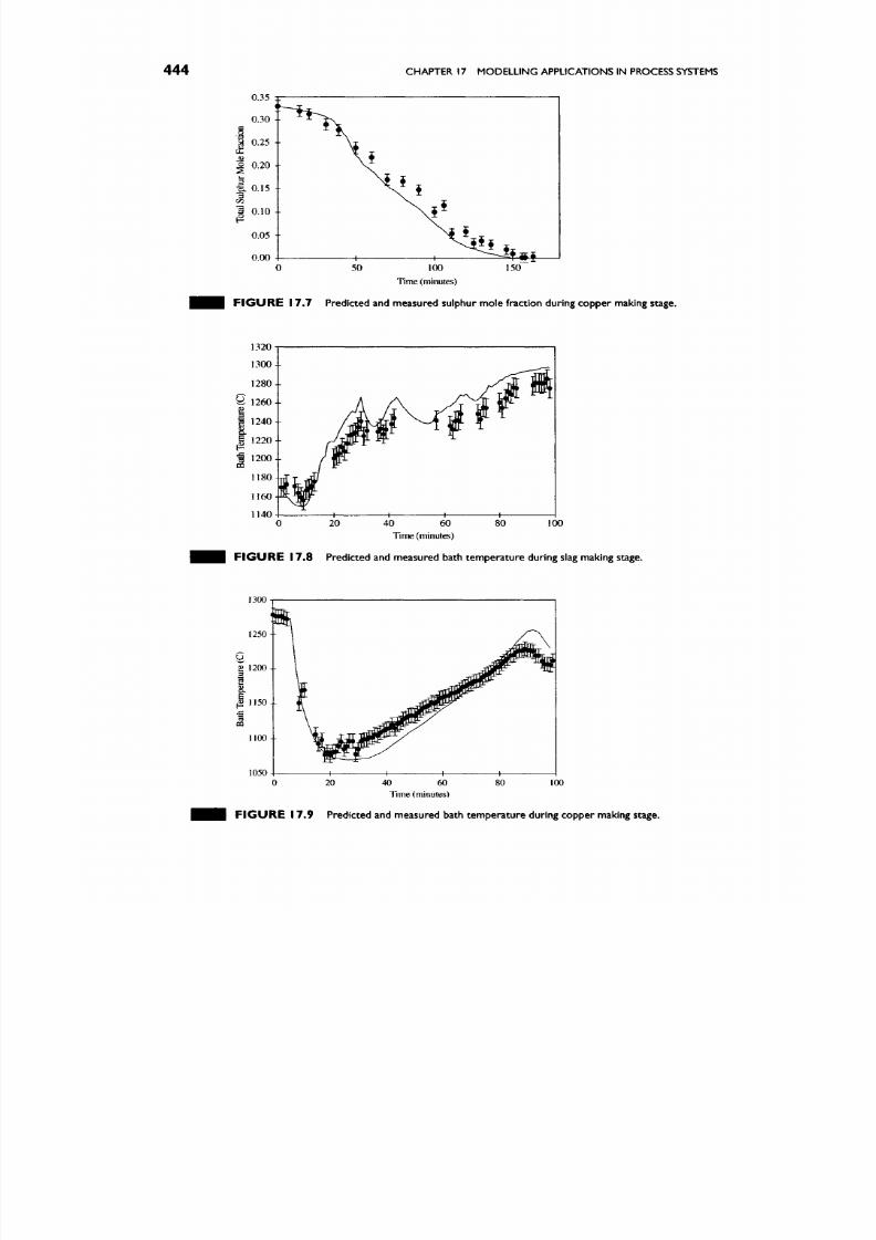
8/17/2019 Process Modelling and Model Analysis-Hangos-Cameron
http://slidepdf.com/reader/full/process-modelling-and-model-analysis-hangos-cameron 461/560
444
CHAPTER 17 MO DELL ING APPLICATIONS IN PROCESS SYSTEMS
100
Time (minutes)
F I G U R E 17 .7 Predicted and measured sulphur mole fraction during copper making stage.
40 60
Tmie (minutes)
100
F I G U R E 17 .8 Predicted and measured bath temperature during slag making stage.
1300
40 60
Time (minutes)
F I G U R E 17 .9 Predicted and measured bath temperature during copper making stage.
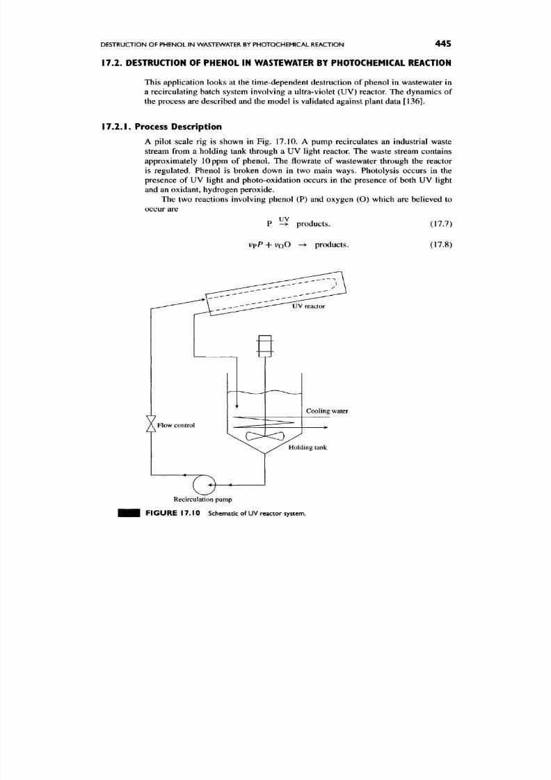
8/17/2019 Process Modelling and Model Analysis-Hangos-Cameron
http://slidepdf.com/reader/full/process-modelling-and-model-analysis-hangos-cameron 462/560
DESTRUCTION OF PHENOL IN WASTEWATER BY PHOTOCHEMICAL REACTION
445
17.2.
DESTRUCTION OF PHENOL IN WASTEWATER BY PHOTOCHEMICAL REACTION
This application looks at the time-dependent destruction of phenol in wastewater in
a recirculating batch system involving a ultra-violet (UV) reactor. The dynamics of
the process are described and the model is validated against plant data
[136].
17.2.1.
Process Description
A pilot scale rig is shown in Fig. 17.10. A pump recirculates an industrial waste
stream from a holding tank through a UV light reactor. The waste stream contains
approximately lOppm of phenol. The flowrate of wastewater through the reactor
is regulated. Phenol is broken down in two main ways. Photolysis occurs in the
presence of UV light and photo-oxidation occurs in the presence of both UV light
and an oxidant, hydrogen p eroxide.
The two reactions involving phenol (P) and oxygen (O) which are believed to
occur are
UV
— > •
products. (17.7)
VpP
+ V Q O
products.
(17.8)
Recirculation pump
F IG U R E 1 7. 10 Schematic of UV reactor system.

8/17/2019 Process Modelling and Model Analysis-Hangos-Cameron
http://slidepdf.com/reader/full/process-modelling-and-model-analysis-hangos-cameron 463/560
446 CHAPTER 17 MODELLING APPLICATIONS IN PROCESS SYSTEMS
Modelling Goal
The model should describe the time varying phenol degradation as a function of
recirculation flowrate and initial concentration of hydrogen peroxide.
17.2.2.
Controlling Factors
The controlling factors for this system are
• chemical reaction due to the UV light,
• radiative heat transfer in the UV light reactor,
• forced convection heat transfer in the recircu lation tank.
17.2.3.
Assumptions
The following assumptions were applied in developing the model:
^ l . Recirculation tank is well mixed.
Al,
No heat losses from tank walls and piping.
^ 3 . Agitator speed is constant and shaft work is negligible.
.44. Cooling coil contents are well mixed.
^ 5 . Liquid holdup in pipelines and reactor is negligible comp ared with the tank.
^ 6 . Kinetic and potential energy effects are negligible.
Al.
Reaction rate constants are independent of temperature over the operating range.
.48. There is no physical mass loss or gain in the system.
^ 9 . Physical properties of the solution are those of water.
^10 . No side reactions occur and no UV reaction occurs outside the reactor.
v411. There is no heat loss from the UV reactor.
AVI. The UV light provides a constant heat source evenly distributed along the
reactor.
.413. For each mole of phen ol, half a mole of hydrogen peroxide is consum ed.
.414.
Heat transfer coefficients are constant.
.415. Coiling coil mass holdup is constant.
17.2.4. Model Development
Three principal balance volumes were identified for the system. These include:
• volume of the UV reactor,
• volume of the recirculation tank,
• volume of the cooling coil within the recirculation tank.

8/17/2019 Process Modelling and Model Analysis-Hangos-Cameron
http://slidepdf.com/reader/full/process-modelling-and-model-analysis-hangos-cameron 464/560
DESTRUCTION OF PHENOL IN WASTEWATER BY PHOTOCHEMICAL REACTION 447
Recirculation Tank Balances
Component balances The component mole balances for phenol (P) and oxidant (O)
are given by
dP r
1
-7 ^ = — (PMR-PTqT)^ (17.9)
at Vj
dO r 1
"TT = Tri^MR -
O T ^ T ) ,
(17.10)
at
Vj
where Pj, Ox are concentrations in [mol/1] and ^R and qj are volumetric flowrates
in
[1/s].
Energy balance
The energy balance in simplified intensive form is given by
dT r
1 Or
— f
=
— iqRTK
-
qjTj)
-
j ^ — (17.11)
at VJ yjpcp
Cooling Coil Balances
The mass balance
is
not required as the h oldup
is
assumed constant (^415).
Energy balance
The energy balance for the cooling coil is given by
dTc 1 Gc
- T -
= TT^qcTcAn - qcTcout) - 7 } ,
(17.12)
dr Vc
Vjpcp
where 7c,in» 7c,out
are the
cooling water temperatures
in and out of
the coil ([K]),
qc
is the cooling water vo lumetric flow ([1/s]).
Lumped Parameter
UV
Reactor Balances
The first approach uses a lumped parameter model of the UV reactor.
Component balances
The component balances are given by
- T T
=
17-(^T^T
-
PRqR) - n - vpr2, (17.13)
at VR
-—
= -j-iOjqj -
OR<7R)
- vo^2. (17.14)
dt VR
Energy balance The energy balance in simplified intensive variable form is given by
^ =
^{qjTj
-
qRTR)
+ — ( r i Af/,, +
r2AHr,)
- - ^ , (17.15)
dt VR pcR VRPCP
where
r\, r2
are reaction rates
for
the two key reactions [mol/1
•
s] ,
A//r, and
AZ/fj
are heats of reaction [J/mol] and QL is the rate of heat transfer from the UV light
[J/s].
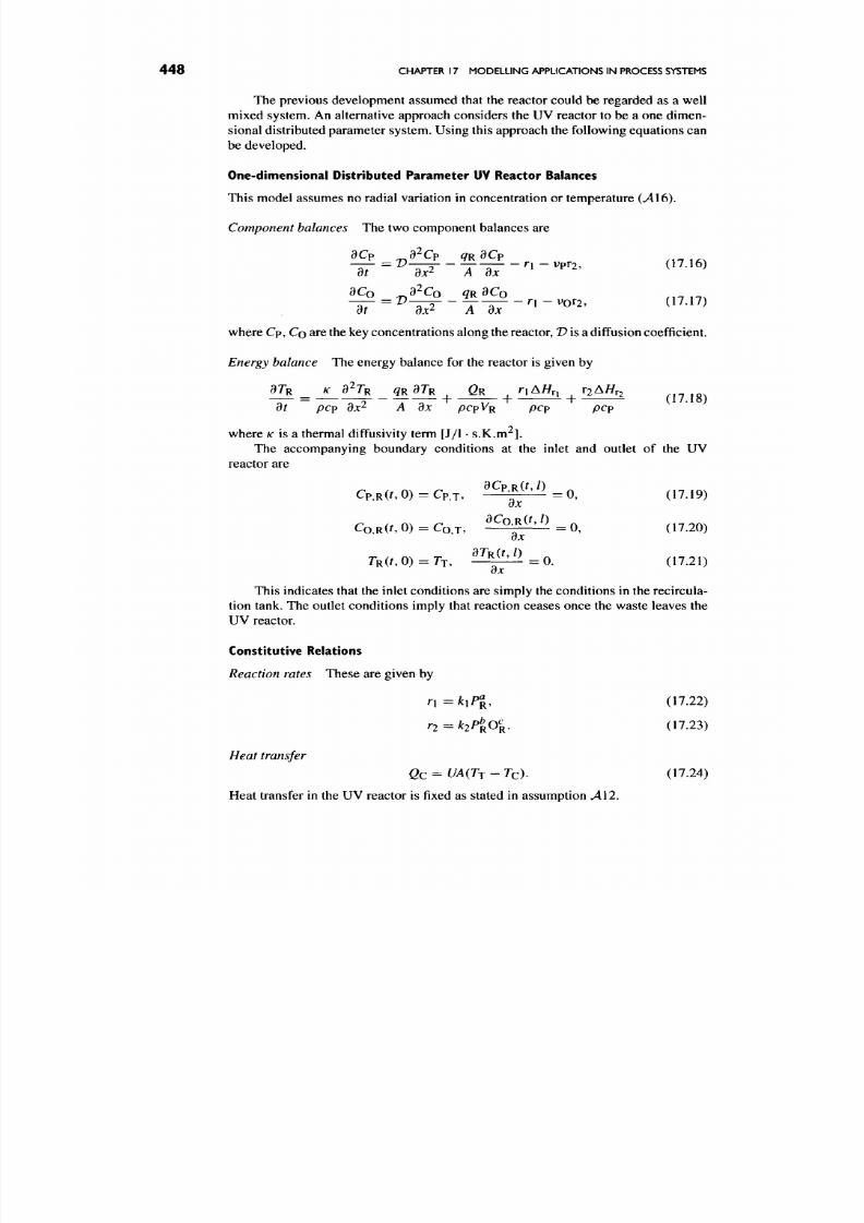
8/17/2019 Process Modelling and Model Analysis-Hangos-Cameron
http://slidepdf.com/reader/full/process-modelling-and-model-analysis-hangos-cameron 465/560
448 CHAPTER 17 MODELL ING APPLICATIONS IN PROCESS SYSTEMS
The previous development assumed that the reactor could be regarded as a well
mixed system. An alternative approach considers the UV reactor to be a one dimen
sional distributed parameter system . Using this approach the following equ ations can
be developed.
One-dimensional Distributed Parameter UV Reactor Balances
This model assumes no radial variation in concentration or temperature (.416).
Component balances The two component balances are
TT =
^""5"2
T~Z
^1 ~ ^P^2, (17.16 )
dt dx^ A dx
where C p, Co are the key concentrations along the reactor, P is a diffusion coefficient.
Energy balance
The energy balance for the reactor is given by
a iR ^ _ ^ a ^ _ ^ OTR ^
QR
^
riAHr,
^ r2Af/r2 ^^ jg
dt pep dx^ A dx pCpVR pep pep
where /c is a thermal diffusivity term [J/1 • s.K.m^].
The accompanying boundary conditions at the inlet and outlet of the UV
reactor are
Cp,R(r,0) = Cp.T, ' .^M^=o, (17.19)
dx
CoMt. 0) - Co,T, ^ f = 0, (17.20)
dx
TR(t,0)
= TT, ^Il^Lll=o. (17.21)
dx
This indicates that the inlet conditions are simply the conditions in the recircula
tion tank. The outlet conditions imply that reaction ceases once the waste leaves the
UV reactor.
Constitutive Relations
Reaction rates These are given by
ri=kiPl (17.22)
r2 = k2PiOi,
(17.23)
Heat transfer
Qc = UA{TT - Tc). (17.24)
Heat transfer in the UV reactor is fixed as stated in assumption ^12.
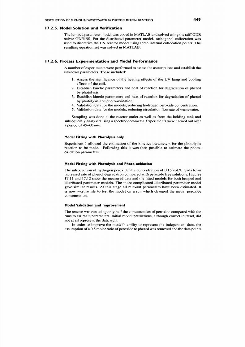
8/17/2019 Process Modelling and Model Analysis-Hangos-Cameron
http://slidepdf.com/reader/full/process-modelling-and-model-analysis-hangos-cameron 466/560
DESTRUCTION OF PHENOL IN WASTEWATER BY PHOTOCHEMICAL REACTION 449
17.2.5. Model Solution and Verification
The lumped param eter model was coded in MATLAB and solved using the stiff OD E
solver ODE15S. For the distributed parameter model, orthogonal collocation was
used to discretize the UV reactor model using three internal collocation points. The
resulting equation set was solved in MATLAB.
17.2.6. Process Experimentation and Model Performance
A number of experiments were performed to assess the assumptions and establish the
unknown param eters. These included:
1.
Assess the significance of the heating effects of the UV lamp and cooling
effects of the coil.
2.
Establish kinetic parameters and heat of reaction for degradation of pheno l
by ph otolysis.
3.
Establish kinetic parameters and heat of reaction for degradation of phenol
by photolysis and photo-oxidation.
4.
Validation data for the mo dels, reducing hydrogen pe roxide co ncentration.
5. Validation data for the models, reducing circulation flowrate of wastewater.
Sampling was done at the reactor outlet as well as from the holding tank and
subsequently analysed using a spectrophotometer. Experiments were carried out over
a period of 45-6 0 min.
Model Fitting with Photolysis only
Experiment 1 allowed the estimation of the kinetics parameters for the photolysis
reaction to be made . Following this it was then possible to estimate the photo-
oxidation parameters.
Model Fitting with Photolysis and Photo-oxidation
The introduction of hydrogen peroxide at a concentration of 0.15 vol.% leads to an
increased rate of phenol degradation compared with peroxide free solutions. Figures
17.11 and 17.12 show the measured data and the fitted models for both lumped and
distributed parameter models. The more complicated distributed parameter model
gave similar results. At this stage all relevant parameters have been estimated. It
is now worthwhile to test the model on a run which changed the initial peroxide
concentration.
Model Validation and Improvement
The reactor was run using only half the concentration of peroxide compared with the
runs to estimate parameters. Initial model predictions, although correct in trend, did
not at all represent the data well.
In order to improve the model's ability to represent the independent data, the
assumption of a 0.5 molar ratio of peroxide to phenol was removed and the data points
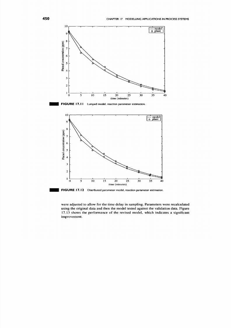
8/17/2019 Process Modelling and Model Analysis-Hangos-Cameron
http://slidepdf.com/reader/full/process-modelling-and-model-analysis-hangos-cameron 467/560
450 CHAPTER 17 MO DEL LING APPLICATIONS IN PROCESS SYSTEMS
15 20 25
time (minutes)
F I G U R E
17 .
M Lumped model, reaction parameter estimation.
40
15 20 25
time (minutes)
40
F I G U R E 17.1 2 Distributed parameter model, reaction parameter estimation.
were adjusted to allow for the time delay in sampling. Param eters were recalculated
using the original data and then the model tested against the validation data. Figure
17.13 shows the performance of the revised model, which indicates a significant
improvement.

8/17/2019 Process Modelling and Model Analysis-Hangos-Cameron
http://slidepdf.com/reader/full/process-modelling-and-model-analysis-hangos-cameron 468/560
PREFERMENTER SYSTEM FOR WA STEWATER TREATM ENT
8r
451
10 15 20 25 30 35 40 45 50
time (minutes)
F I G U R E 17 .13 Full lumped parameter model preformance.
17.3.
PREFERMENTER SYSTEM FOR WASTEWATER TREATMENT
This example considers the dynamics of a prefermenter unit used in a wastewater
treatment facility.
17.3.1.
Process Description
Prefermentation is a relatively new operation in biological nutrient removal (BN R) of
wastewater treatment systems. The prefermentation role is to produce volatile fatty
acids (VFAs) which assist in the subseque nt removal of nitrogen and phospho rus from
the wastewater. The prefermenter relies on comp lex biological reactions taking place
producing VFAs via an anaerobic degradation process. The dynamic modelling of
these systems has recently been completed by von Miinch [137]. A schematic of the
overall process is seen in Fig. 17.14.
Modelling Goal
The goal is to predict the dynamic behaviour of VFA production, pH and soluble
chemical oxygen demand (SCOD) under the influence of changing wastewater feed
composition or flow.
17.3.2.
Controlling Factors
Key factors in the system include:
• two major processes of hydrolysis and acidogene sis take place ;
• hydro lysis is catalysed via hydrolytic enzymes excreted by bacteria;
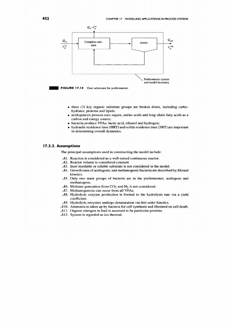
8/17/2019 Process Modelling and Model Analysis-Hangos-Cameron
http://slidepdf.com/reader/full/process-modelling-and-model-analysis-hangos-cameron 469/560
452
CHAPTER 17 MOD ELLING APPLICATIONS IN PROCESS SYSTEMS
G in
1
p ;
Q ,C^
Complete-mix
tank
A
Sett
pr
Gout
/^OUt
Prefermenter system
and model boundary
F I G U R E 17.14 Ov er schematic for prefermenter.
three
(3) key
organic substrate groups
are
broken dow n, including carbo
hydrates, proteins and lipids;
acidogenesis process uses sugars, amino acids and long chain fatty acids as
a
carbon and energy source;
bacteria produce VFAs, lactic acid, ethanol and hydrogen;
hydraulic residence time (HR T) and solids residence time (SRT) are important
in determining overall dynamics.
17.3.3. Assumptions
The principal assumptions used in constructing the model include:
A\. Reaction is considered as
a
well-mixed continuous reactor.
A2. Reactor volume is considered constant.
Ai.
Inert insoluble or soluble substrate
is
not considered
in
the model.
.44. Growth rates of acidogenic and methanogenic bac teria are described by Monod
kinetics.
^ 5 . Only two main groups of bacteria are in the prefermenter, acidogens and
methanogens.
A6.
M ethane generation from CO2 and H2 is not co nsidered.
Al. M ethanogenesis can occur from all VFA s.
v48. Hydrolytic enzyme production is limited to the hydrolysis rate via a yield
coefficient.
A9.
Hydrolytic enzymes undergo denaturation via first order kinetics.
^ 1 0 . Am mon ia is taken up by bacteria for cell synthesis and liberated on cell death.
^ 1 1 . Organ ic nitrogen in feed is assumed to be particular proteins.
All. System is regarded as iso-thermal.

8/17/2019 Process Modelling and Model Analysis-Hangos-Cameron
http://slidepdf.com/reader/full/process-modelling-and-model-analysis-hangos-cameron 470/560
PREFERMENTER SYSTEM FOR WASTEWATER TREATMENT
453
173.4. Model Development
In developing the model, balances in the system of Fig. 17.14 relate to
• solids (insoluble substrate, biom ass, proteins ),
• liquid components (soluble substrate, VFA, enzymes).
Mass B alances
The solid mass balances become
V R ^ = QinC'^j - Q^C^i - QoutC^l + V^J2 ^Ji^h (17.25)
where VR is the prefermenter reactor volume [litres], Cp,/ the particulate compon
ent / concentration [mg/1],
Q
the flowrate of stream [m^/h],
Vji
the stoichiometric
coefficient for component / in process7, T lj is the rate equation for process7.
Liquid Component Balances
At
J
(17.26)
The structure of the prefermenter model is shown in Fig. 17.15 where the
individual species definitions are given in Table 17.1.
Solid lines show COD mass balances and dashed lines represent nitrogen
mass balances. Y^ represents yields for various reactions k, Y^/x are stoichiometric
ammonia-N requirements for biomass synthesis and r represent the various reaction
rates.
FIGURE 17 .15 Prefermenter model structu re.
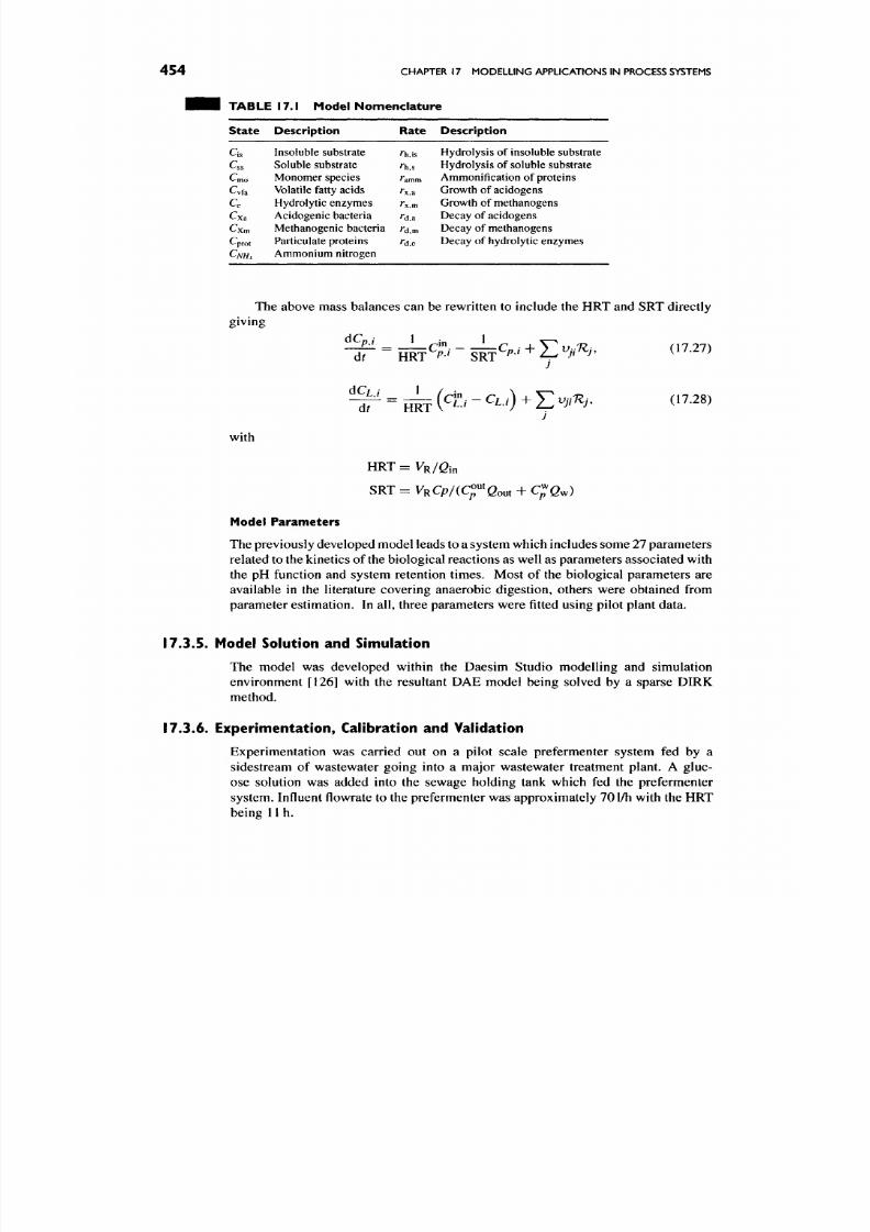
8/17/2019 Process Modelling and Model Analysis-Hangos-Cameron
http://slidepdf.com/reader/full/process-modelling-and-model-analysis-hangos-cameron 471/560
454 CHAPTER 17 MODELLING APPLICATIONS IN PROCESS SYSTEMS
• ^ H l TABLE 17.1 Model Nomenclature
State
^ i s
^ s s
^ m o
^ v f a
Ce
Cxa
Cxm
^prot
CNHA
Description
Insoluble substrate
Soluble substrate
Monomer species
Volatile fatty acids
Hydrolytic enzymes
Acidogenic bacteria
Methanogenic bacteria
Particulate proteins
Ammonium nitrogen
Rate
^h,is
^h.s
' 'amm
rx,a
fx,m
rd,a
' 'd .m
' 'd .e
Description
Hydrolysis of insoluble substrate
Hydrolysis of soluble substrate
Ammonification of proteins
Growth of acidogens
Growth of methanogens
Decay of acidogens
Decay of methanogens
Decay of hydrolytic enzymes
The above mass balances can be rewritten to include the HRT and SRT directly
giving
d? HRT ''•' SRT
;,i-^^Cpj + J2vjiTlj, (17.27)
with
J
HRT = VR/Gin
SRT = Vj^Cp/iC^'^'Qoui + C^Qv^)
(17.28)
Model Parameters
The previously developed model leads to a system w hich includes some 27 parameters
related to the kinetics of the biological reactions as well as parameters associated w ith
the pH function and system retention times. Mo st of the biological parameters are
available in the literature covering anaerobic digestion, others were obtained from
parameter estimation. In all, three parameters w ere fitted using pilot plant data.
17.3.5. Model Solution and Simulation
The model was developed within the Daesim Studio modelling and simulation
environment [126] with the resultant DAE model being solved by a sparse DIRK
method.
17.3.6. Experimentation, Calibration and Validation
Experimentation was carried out on a pilot scale prefermenter system fed by a
sidestream of wastewater going into a major wastewater treatment plant. A gluc
ose solution was added into the sewage holding tank which fed the prefermenter
system. Influent flow rate to the prefermenter w as approximately 701/h with the HRT
being
11
h.

8/17/2019 Process Modelling and Model Analysis-Hangos-Cameron
http://slidepdf.com/reader/full/process-modelling-and-model-analysis-hangos-cameron 472/560
PREFERMENTER SYSTEM FOR WASTEWATER TREATMENT
455
The system was then analysed over the next 60 h and the mode l pred ictions
compared with the plant data. Figures 17 .16-17.18 show a comparison of model
predictions with the plant data indicating a good prediction of the system dynamics
for VFA, SCOD and Ph.
The model provides a reasonable basis for further detailed control and design
studies.
250
200
Q
O
U
>
100
50
0
1 1 —
o
+
of*
[
7 ^ H
+:"
+:
y o
\
^
[
+
+
1 1 1
0
+
o
+
_,
o
+
1 : '
— model output
o plant output
+ plant input
simulated input J
•1
1 _..,-.. 1. .. 1
64 65
F I G U R E 1 7 . 1 6 VFA pred iction versus plant data.
66 67 68
time (day)
69
70
600
5 h
400
S 300
Q
O
u
00
200
100
64
65
r
-
1 )
1 ^
r +
:
+
1—
+
+A
1
^
1
°
' o
V
\ o
; + +
:+
1 1 1
O
^ " ^ ^ - - . ^ O
+
+
1 1 —
1 1 ,
— model output
0 plant output
+ plant input
simulated input N
H
J
d
•j
J
66 67 68
time (day)
69
70
F I G U R E 1 7 . 1 7 SCOD predictions versus plant data.
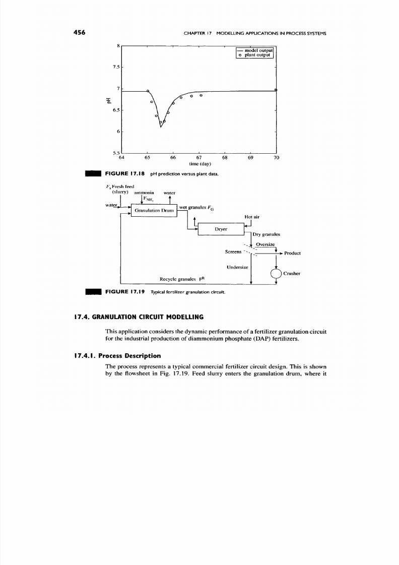
8/17/2019 Process Modelling and Model Analysis-Hangos-Cameron
http://slidepdf.com/reader/full/process-modelling-and-model-analysis-hangos-cameron 473/560
456 CHAPTER 17 MODELLING APPLICATIONS IN PROCESS SYSTEMS
8
7.5
7
6.5
6
-
o\
o\ /
y b
1 1
0 O
1 . . . „ 1
, 1 .~1
— model output
o plant output | |
J
, Vf
1
1 1
64 65 66 67 68
time (day)
F I G U R E 1 7 . 1 8 pH prediction versus plant data.
Fs Fresh feed
(slurry) ammonia water
1^-- t
69 70
water^
Granulation Drum
wet granules F^
Hot air
Dryer
Dry granules
^1 Oversize
Screens
Undersize
Recycle granules F*^
- • Product
( j Crusher
FIGURE 17 .19 Typical fertil izer granulation circu it.
I 7 A GRANULATrON CIRCUrT MODELLING
This application con siders the dynamic performanc e of a fertilizer granu lation circuit
for the industrial production of diammonium phosphate (DAP) fertilizers.
17.4.1.
Process Description
The process represents a typical commercial fertilizer circuit design. This is shown
by the flowsheet in Fig. 17.19. Feed slurry enters the granulation drum, where it

8/17/2019 Process Modelling and Model Analysis-Hangos-Cameron
http://slidepdf.com/reader/full/process-modelling-and-model-analysis-hangos-cameron 474/560
GRANULATION CIRCUIT MODELLING 4 5 7
mixes with recycled fertilizer granules which are normally in the undersize range.
This recycle consists of either true undersize material or crushed oversize from the
screening operation. Product from the granulator is fed to a high temperature dryer
for moisture reduction and consolidation before passing through a series of screens
which separate out the product size (3-5 m m d iameter). Undersize goes directly into
the recycle stream and oversize passes through a crusher then into the recycle stream
for return to the granulator.
Operation of commercial granulation circuits is prone to problems of large vari
ability and poor stability. Development of advanced control strategies is important
for addressing productivity issues.
Modelling Goal
To predict the circuit dynamics in the face of disturbances in feed rate and moisture
in order to test control schemes for improved circuit performance.
17.4.2.
Controlling Factors
In this application, there are several controlling factors:
• granule growth within the granulator drum, w hich is both moisture and size
dependent;
• particulate drying within the rotary dryer;
• screening of particles in vibratory screen system;
• hamm er mill crusher performance for particle reduc tion;
• transportation delays in granulator, dryer and recycle systems .
17.4.3. Assumptions
The principal assumptions are:
^ 0 . No nucleation occurs in the slurry.
>t l . All remaining MAP reacts with ammonia fed to the granulator.
A2. Particles only undergo coalescence due to surface liquid being present.
^ 3 .
Layering occurs first in the drum then coalescence.
A4.
No particle breakage is considered.
^ 5 .
Operating temperature along the drum is constant.
17.4.4. Model Development
The key unit in the flowsheet is the granulator. Here a number of mechanisms are
important such as
• reaction
• layering
• coalescence
The reaction is exothermic with ammonia reacting with mono-ammonium
phosphate (MAP) to form DAP and liberating water.

8/17/2019 Process Modelling and Model Analysis-Hangos-Cameron
http://slidepdf.com/reader/full/process-modelling-and-model-analysis-hangos-cameron 475/560
458
CHAPTER 17 MODELLING APPLICATIONS IN PROCESS SYSTEMS
Layering occurs which increases particle mass but not particle number, whilst
coalescence affects particle number.
Overall Mass Balance
Here slurry, recycle and fresh ammonia combine to give wet granules and water
F^+F^ + pfjH, ^F°+ F^^Z-
(17-29)
Granule Mass Balance
Fresh DAP includes DAP in the slurry plus the formation from MAP.
^DAP = ^DAP + (^MAP + ^NH^)- (17.30)
The total DAP includes both fresh and recycled
^DAP
=
^DAP
+
^DAP (17.31)
Particle Population Balance
Using volume
of
particle
as the
internal co-ordinate
it is
possible
to
discretize
the continuous volume domain into a geometric series as described by Hounslow
etal. [128].
The particle population balance is given by
at dz
where birth and death terms are
B]'^ = J22'-'^^Pi-ljNi-xNj (17.33)
birth in ith interval from coalescence of particle in (/ — l)th interval
with particles in first to
(/
— 2)th interval
^ P = l)0,_i,/_iA^/_iA^,_i (17.34)
birth in
ith
interval from two particles in
(/
—
l)th interval
i-l
Df^=Y.2J-^Pi^jNiNj
(17.35)
death of particle in
ith
interval due to coalescenc e with particle in first
to(/
- \)th
interval
00
death in
ith
interval due to coalescence between particle in interval
with a larger particle.
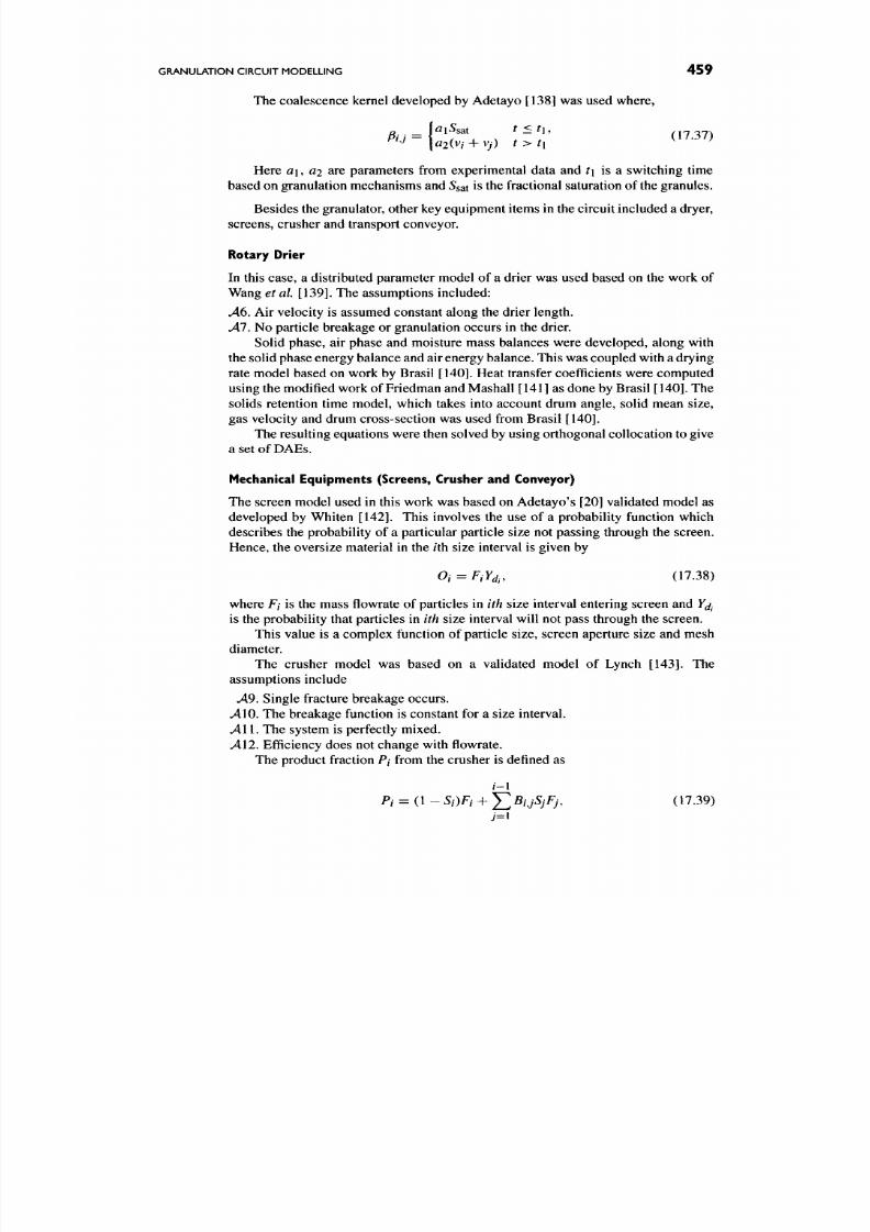
8/17/2019 Process Modelling and Model Analysis-Hangos-Cameron
http://slidepdf.com/reader/full/process-modelling-and-model-analysis-hangos-cameron 476/560
GRANULATION CIRCUIT MODELLING 4 5 9
The coalescence kernel developed by Ad etayo [138] was used wh ere,
Here
a\, ai
are parameters from experimental data and
t\
is a switching time
based on gran ulation m echanism s and 5sat is the fractional saturation of the granules.
Besides the granulator, other key equipmen t items in the circuit include d a dryer,
screens, crusher and transport conveyor.
Rotary Drier
In this case, a distributed parameter model of a drier was used based on the work of
Wang
et
al. [139]. The assumptions included:
A6.
Air velocity is assumed constant along the drier length.
Al.
No particle breakag e or granulation occurs in the drier.
Solid phase, air phase and moisture mass balances were developed, along with
the solid phase energy balan ce and air energy balance. This w as coupled w ith a drying
rate model based on work by Brasil [140]. Heat transfer coefficients were computed
using the modified w ork of Friedman and Mashall [141] as done by Brasil
[140].
The
solids retention time model, which takes into account drum angle, solid mean size,
gas velocity and drum cross-section was used from Brasil [140].
The resulting equations were then solved by using orthogonal c ollocation to give
ase tof DAEs.
Mechanical Equipments (Screens, Crusher and Conveyor)
The screen model used in this work was based on Adetayo's [20] validated model as
developed by Whiten [142]. This involves the use of a probability function which
describes the probability of a particular particle size not passing through the screen.
Hence, the oversize material in the iih size interval is given by
Oi =
FiYd., (17.38)
where F/ is the mass flowrate of particles in ith size interval entering screen and Y^.
is the probability that particles in
ith
size interval will not pass through the screen.
This value is a complex function of particle size, screen aperture size and mesh
diameter.
The crusher model was based on a validated model of Lynch [143]. The
assumptions include
A9.
Single fracture breakage occurs.
^ 1 0 . The breakage function is constant for a size interval.
All.
The system is perfectly mixed.
^ 1 2 . Efficiency does not change with flowrate.
The product fraction P/ from the crusher is defined as
/ - I
Pi
= (1 -
Si)Fi
+ Y.^i,jSjFj, (17.39)
7 = 1

8/17/2019 Process Modelling and Model Analysis-Hangos-Cameron
http://slidepdf.com/reader/full/process-modelling-and-model-analysis-hangos-cameron 477/560
460 CHAPTER 17 MODELLING APPLICATIONS IN PROCESS SYSTEMS
where Bjj is the breakage function, being the p robability of a particle in the ith size
interval being broken into particles less than the top size in the ith size interval.
The selection function 5/ represents the probability that a particle in the ith size
interval is selected for breakage. Below a certain size, low there is no selection.
Abo ve 5upp
all
particles
are
selected
for
breakage.
The final model is that for a conveyor system. In this case, the mass balance gives
- -y.f.
( . 7 . 4 0 ,
dt
dz
where M is the particle mass holdup per unit belt length, and V\y is the belt velocity.
This model can be discretized using finite differences or collocation methods for
solution.
17.4.5. Model Solution
The individual models were built into the library structure of the dynamic simula
tion and modelling system Daesim Studio [126]. The overall flowsheet included all
processing units plus control equipment such as sensors, controllers and actuators.
The large, sparse DAE system of equations was then solved using BD F and DIRK
methods.
17.4.6. Model Experimentation
The model was built with the purpose of examining the overall circuit dynamics,
effects of drier and crusher characteristics and to examine possible standard or
advanced co ntrol applications. Several case studies were carried out to assess control
performance
of
various strategies.
The case studies included:
• Feedback only control using the water content of the feed slurry as the manip
ulative variable whilst using the fraction of oversize and undersize particles in
the recycle for control purposes.
• Feedforward only control based on a simplified model of the granulator
moisture as a function of the key stream properties.
• A combined feedforw ard-feedback controller which used a simplified pro
cess model for the feedforward part and feedback control to compensate for
inaccuracies in the process model and unmeasured disturbances.
In the first case study, slurry flowrate was increased by 10%, whilst the A^:P
ratio was decreased
by
5%.
Figure 17.20 shows the predicted responses of the circuit to such changes and
the performance of the control strategies. The increase in slurry flow, with water
input initially at the steady operating conditions leads to a significant increase in
undersize m aterial in the recycle. The predictions show the relative performance of the
three control strategies with superior performance d emonstrated by the feedforw ard-
feedback strategy. Significant time delays in the granulator, drier and recycle system
contribute to the difficulty of circuit control.
The second study considered
a
simulated partial blockage
in
recycle from
a
time
of 10 min to 60 min leading to a reduction in recycle flow of 10%. Figure 17.21
shows the responses of the under-size m ass fraction in the recycle for various control
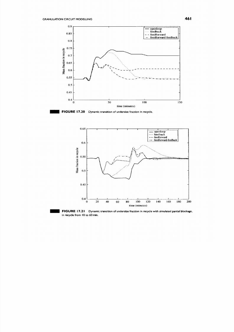
8/17/2019 Process Modelling and Model Analysis-Hangos-Cameron
http://slidepdf.com/reader/full/process-modelling-and-model-analysis-hangos-cameron 478/560
GRANULATION CIRCUIT MODELLING
0.9
0.85
0.8
jj
0.75
o
^ 0.7
I
0.65
S 0.6
0.55
0.5
0.45
0.4
461
0
1
^ ^ . ^ ^ ^
l\ ^\-~, \
\J ^- Z\...
1 1
— ope n l oop 1
• feedback
— feedforward 1
- feedforward feedback |
H
H
1
50
100
150
time (minutes)
F I G U R E 1 7 , 2 0 Dynamic transition of undersize fraction In recycle.
0.65
0.6
.S 0.55
h
0.5
0.45
0.4
1 1 1
1 1 1
1 1
1 1
\
1 1
— openloop
— feedback
— feedforward
— feedforward-feedback
1 1 1 1
H
0
2 0 4 0 6 0 8 0 1 0 0 12 0 14 0 16 0 180 2 0 0
time minutes)
FIGURE 17 .21 Dynamic transition of undersize fraction In recycle with simulated partial blockage,
In recycle fro m
10
t o
60 min.
8/17/2019 Process Modelling and Model Analysis-Hangos-Cameron
http://slidepdf.com/reader/full/process-modelling-and-model-analysis-hangos-cameron 479/560
462 CHAPTER 17 MODELLI NG APPLICATIONS IN PROCESS SYSTEMS
Strategies. Ag ain, the feedforward-feedback strategy performs better than the simpler
control approaches such as feedback or purely feedforward.
The study w as able to identify a number of promising strategies for circuit control
which considered a range of potential control and manipulated variables. The model
has also been used to study the application of model predictive control (MPC) to the
circuit.
17.5. INDUSTRIAL DEPROPANIZER USING STRUCTURAL PACKING
This example discusses the modelling of an industrial depropanizer as part of an oil
refinery. In this case, the tower uses a structured packing and the modelling leads to
a distributed parameter system. The model uses a rate based approach in developing
the dynamic description of the process [144,145].
17.5.1.
Process Description
Depropanizers are often used in refinery processing. In this case, the column is an
integral part of an alkylation unit. Here, the modelling is required to help derive
improved control under the influence of large disturbances on the system.
17.5.2.
Controlling Factors
Key factors in this system are
• the use of structured packing (Sulzer Mellapak 250/300) in top and bottom
sections of the column;
• mass and heat transfer in packed column operations;
• importance of major ho ldups in the system including the reboiler and reflux
drum;
• the number of individual com ponents to be considered in the model versus
plant.
17.5.3.
Assumptions
The main assumptions include:
Al,
The vapour phase holdup is regarded as negligible.
A2, No significant heat losses from the column or associated equipmen t.
.43. Simplified Stefan-Maxwell equations are applicable and represented by
Wilke's equation.
A4.
Mass and heat transfer represented by correlations.
^ 5 . Pressure profile is considered cons tant.
A6.
Thermal capacity of the column and packing are negligible.
Al. No chemical reactions occur.
.48. No variation in the radial direction.
A9. Assum e simple relationship between liquid flow and holdup .
.410. Assum e liquid-v apou r interface is at equilibrium for the two-film m odel.
.411.
No significant heat of mixing in the system.
.412. Vapour phase controls the mass transfer rate.
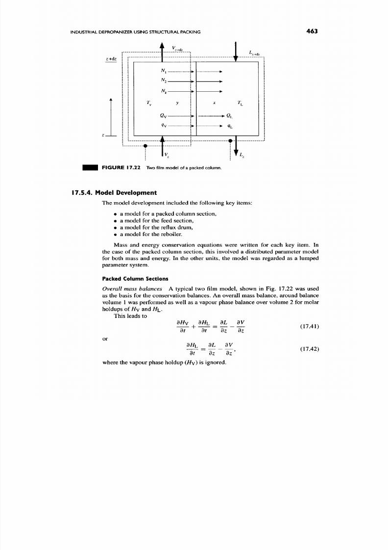
8/17/2019 Process Modelling and Model Analysis-Hangos-Cameron
http://slidepdf.com/reader/full/process-modelling-and-model-analysis-hangos-cameron 480/560
INDUSTRIAL DEPROPANIZER USING STRUCTURAL PACKING
463
z+dz
I
+iU
9v-
i
z+dz
t
F IG U R E 17.22 Two film model of a packed column.
17.5.4. Model Development
The model development included the following key items:
• a mod el for a packed column section,
• a mod el for the feed section,
• a mod el for the reflux drum,
• a model for the reboiler.
Mass and energy conservation equations were written for each key item. In
the case of the packed column section, this involved a distributed parameter model
for both mass and energy. In the other units, the model was regarded as a lumped
parameter system.
Packed Column Sections
Overall mass balances A typical two film mo del, shown in Fig. 17.22 was used
as the basis for the conservation balances. An overall mass balance, around balance
volume 1 was performed as well as a vapour phase balance over volume 2 for molar
holdups of//v and
H\^.
This leads to
dt
dt
dz dz
or
dt
3l
a 7 '
(17.42)
where the vapour phase holdup (/ /y) is ignored.

8/17/2019 Process Modelling and Model Analysis-Hangos-Cameron
http://slidepdf.com/reader/full/process-modelling-and-model-analysis-hangos-cameron 481/560
464 CHAPTER 17 MODELLING APPLICATIONS IN PROCESS SYSTEMS
For the vapour phase, we obtain
dt
dz ^ ,
or
^^
k=\
when the vapour holdup is negligible. Here, N^ is the molar flux of component k
between vapour and liquid phases,
A
is the interfacial area of the packing and
S
is the
column.
Compon ent balances Com ponent balances for C — 1 components w ere also needed.
These were written for both liquid and vapour phases as
^AHLXk)
=
^(Lxk)
-
^(Vyk)
(17.45)
dt dz dz
and
0=- Vyk)-Nk (17.46)
dz
which neglects vapour holdup.
Energy balance The overall energy balance is obtained from balance volume 1 as
^(HLh -\- HyH) =^(Lh) - {VH) (17Al)
dt
dz dz
or
| - ( / / L / ^ ) = (Lh) - (VH) (17.48)
dt dz dz
by neglecting vapour holdup.
The vapour phase energy balance over volume 2 gives
0==- VH)-Qv-qv
dz
which ignores the vapour holdup and also accounts for the convective heat transfer
to the liquid phase (gv) and the conductive heat transfer (^v)-
Noting that there is no accumulation of energy at the interface we can write
QL-qL
=
Qy-qw
(17.49)
so that the final energy balance is
C C
J2 NiHi +qw =
t
Nihi + ^L (17.50)
( = 1 1 = 1

8/17/2019 Process Modelling and Model Analysis-Hangos-Cameron
http://slidepdf.com/reader/full/process-modelling-and-model-analysis-hangos-cameron 482/560
INDUSTRIAL DEPROPANIZER USING STRUCTURAL PACKING 465
Constitutive Equations
There are many constitutive equations required in the mod el w hich relate to rate
expressions, property definitions and equilibrium relations. The key constitutive
equations include:
Mass transfer
This can be defined as
Nk
= (KoG)kA'S'(yk-yl), (17.51)
where
KQQ
is the overall gas phase mass transfer coefficient which can be defined
using the Onda [146] correlations and the Bravo, Rocha and Fair correlations [147]
or from Speigel and Meier [148] with
1 1 m.
= 1 L- (17.52)
and the effective liquid and vapour phase coefficients being given using the previous
correlations.
Heat transfer
Heat transfer coefficients w ere estimated using the Ch ilton-C olbu rn
analogy, such that:
h^=klc;(Le'')y\ (17.53)
h^ = it^^C^(Le ^)^/^ (17.54)
where
C
4 = E ^ ' < e f f (17.55)
c
4-E^ '^J :ef f (17.56)
i=\
The convective and conductive heat transfer terms are given by
C
Gv
=
E ^ ^ ^ k , (17.57)
Qh =
Y. khy,
(17.58)
k=\
qw
=
h^ASiTy
-
TO,
(17.59)
qL = h^AS(Ti - TO (17.60)
Phase equilibrium To com pute the interfacial equilibrium com positions }^ , we use
y*k = ^ ^ ^ - ^ - ^ i t . (17-61)
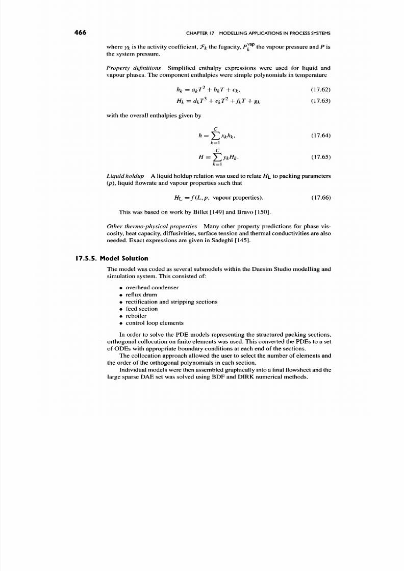
8/17/2019 Process Modelling and Model Analysis-Hangos-Cameron
http://slidepdf.com/reader/full/process-modelling-and-model-analysis-hangos-cameron 483/560
466 CHAPTER 17 MODELLING APPLICATIONS IN PROCESS SYSTEMS
where yi^ is the ac tivity coefficient,
J^f^
the fugacity, P^^ the vapour pressure and
P
is
the system pressure.
Property definitions
Simplified enthalpy expressions were used for liquid and
vapour phases. The component enthalpies were simple polynomials in temperature
hj, =
QkT' +
b^ T
4- Cjt, (17 .62)
Hk = dkT^-^ekT^+fkT + 8k (17.63)
with the overall enthalpies given by
C
h = J2^khk, (17.64)
^=1
c
H = J2ykHk.
(17.65)
Liquid holdup A liquid holdup relation was used to relate / /L to packing parameters
(p), liquid flowrate and vapour properties such that
Hh =f(L,p, vapour properties). (17.66)
This was based on work by Billet [149] and Bravo [150].
Other thermo-physical properties
Many other property predictions for phase vis
cosity, heat capacity, diffusivities, surface tension and thermal conductivities are also
needed. Exact expressions are given in Sadeghi [145].
17.5.5. Model Solution
The model was coded as several submodels within the Daesim Studio modelling and
simulation system. This consisted of:
• overhead condenser
• reflux drum
• rectification and stripping sections
• feed section
• reboiler
• control loop elements
In order to solve the PDE models representing the structured packing sections,
orthogonal c ollocation on finite elements w as used. This converted the PDEs to a set
of ODEs with appropriate boundary conditions at each end of the sections.
The collocation approach allowed the user to select the number of elements and
the order of the orthogonal polynomials in each section.
Individual models w ere then assembled graphically into a final flowshe et and the
large sparse DAE set was solved using BDF and DIRK numerical methods.
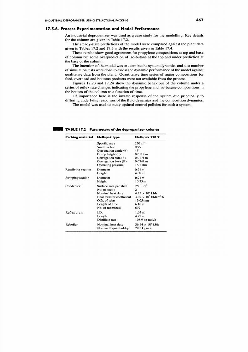
8/17/2019 Process Modelling and Model Analysis-Hangos-Cameron
http://slidepdf.com/reader/full/process-modelling-and-model-analysis-hangos-cameron 484/560
INDUSTRIAL DEPROPANIZER USING STRUCTURAL PACKING
467
17.5.6.
Process Experimentation and Model Performance
An industrial depropanizer was used as a case study for the modelling. Key details
for the column are given in Table 17.2.
The steady-state predictions of the model were compared against the plant data
given in Tables 17.2 and 17.3 with the results given in Table 17.4.
These results show good agreement for propylene compositions at top and base
of column but some overprediction of iso-butane at the top and under prediction at
the base of the column.
The intention of the model w as to examine the system dynam ics and so a number
of simulation tests were done to assess the dynam ic performance of the model against
qualitative data from the plant. Quantitative time series of major com positions for
feed, overhead and bottoms products were not available from the process.
Figures 17.23 and 17.24 show the dynamic behaviour of the column under a
series of reflux rate changes indicating the propylene and iso-butane compositions in
the bottom of the column as a function of time.
Of importance here is the inverse response of the system due principally to
differing underlying responses of the fluid dynamics and the composition dynamics.
The model was used to study optimal control policies for such a system.
TABLE 17.2 Param eters of the depropanizer column
Packing material Mellapak typ e
Mellapak 250 Y
Rectifying section
Stripping section
Condenser
Reflux drum
Reboiler
Specific area
Void fraction
Corrugation angle (0)
Crimp height (h)
Corrugation side (S)
Corrugation base (B)
Operating pressure
Diameter
Height
Diameter
Height
Surface area per shell
No. of shells
Nominal heat duty
Heat transfer coefficient
O.D.of tube
Length of tube
No. of tube/shell
I.D.
Length
Distillate rate
Nom inal heat duty
Nominal liquid holdup
250 m- i
0.95
45°
0.0119 m
0.0171m
0.0241 m
16.1 atm
0.91m
4.08 m
0.91m
10.35
m
250.1 m
2
4.23 X lO^kJ/h
3.02 X lO^kJ/hm^K
19.05 mm
6.10m
697
1.07 m
4.72 m
108.9 kg mol/h
36.94 X lO^kJ/h
2 8 . 3 k g m o l
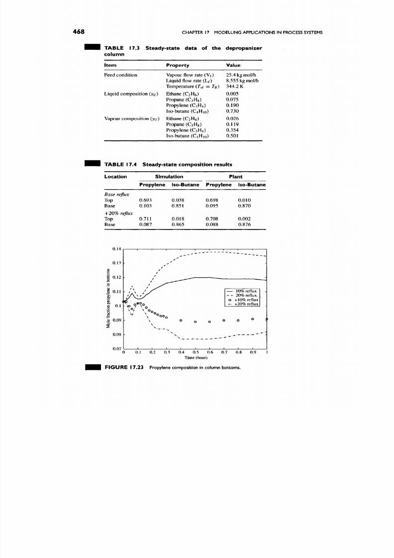
8/17/2019 Process Modelling and Model Analysis-Hangos-Cameron
http://slidepdf.com/reader/full/process-modelling-and-model-analysis-hangos-cameron 485/560
468
CHAPTER 17 MO DEL LING APPLICATIONS IN PROCESS SYSTEMS
TA BL E 17.3 Steady-state da ta of the de prop anizer
c o l u mn
I tem
Property
Value
Feed condition Vapour flow rate (Vf) 25.4 kg mol/h
Liquid flow rate (Lf) 8.555 kg mol/h
Temperature (T^f = Tu ) 344.2 K
Liquid composit ion (XK) Ethane (C2H6)
0.005
Propane (C3H8) 0.075
Propylene (C3H6) 0.190
Iso-butane (C4H10)
0.730
Vapour composition (yif)
Ethane (C2H6)
Propane (CiHg)
Propylene (C3H6)
Iso-butane (C4H10)
0.026
0.119
0.354
0.501
TA BL E 17.4 Steady-state com posit ion results
Location
Base reflux
Top
Base
+20%
reflux
Top
Base
Simulation
Propylene
0.693
0.103
0.711
0.087
iso-Butane
0.038
0.851
0.018
0.865
Plant
Propylene
0.698
0.095
0.708
0.088
iso-Butane
0.010
0.870
0.002
0.876
0.14
0.13 I-
B
§ 0.12
g 0.11
1
2
ex
a
0.1
I
M 0.09
o
0.08
0.07
r - • - — 1 — — 1 1 1 T — 1 1 1 — 1
/
•
/
/ ^
\_
' s
'N.
r 'N_
1 1 1 1 1 1
0
-L -
0
_ L
—
10%
reflux
- -
20%
reflux
0 +10% reflux
-• +20% reflux
0 0
— 1 , — 1 ,
\
k
0 0.1 0.2 0.3 0.4 0.5 0.6 0.7 0.8 0.9 1
Time (hour)
F I G U R E 17 .23 Propylene composition in column bottoms.

8/17/2019 Process Modelling and Model Analysis-Hangos-Cameron
http://slidepdf.com/reader/full/process-modelling-and-model-analysis-hangos-cameron 486/560
SUMMARY
469
0.89
— 10% reflux
— 20% reflux
o +10% reflux
— +20% reflux
0.1 0.2 0.3 0.4 0.5 0.6 0.7 0.8 0.9
Time (hour)
FIGURE 17 .24 Iso-butane compositions in column bottom s.
17.6. SUMMARY
This chapter has presented some examples of industrial modelling practice. The
models displayed in the chapter cover a range of process applications and also model
characteristics. What is evident in these examples is the often difficult problems in
obtaining good plant data for calibration and validation purposes as well as the need
to make simplifying assumptions in order to make the modelling process tractable.
Inevitably in the modelling of real world problems for a range of applications, the
required model fidelity needs to be assessed so that there is a clear endpoint to the
modelling effort.

8/17/2019 Process Modelling and Model Analysis-Hangos-Cameron
http://slidepdf.com/reader/full/process-modelling-and-model-analysis-hangos-cameron 487/560
This Page Intentionally Left Blank
8/17/2019 Process Modelling and Model Analysis-Hangos-Cameron
http://slidepdf.com/reader/full/process-modelling-and-model-analysis-hangos-cameron 488/560
COMPUTER AIDED PROCESS
MODELLING
This chapter discusses the general principles behind the development of computer
based model building environments—or com puter aided process modelling (CA PM)
systems. Recognition is given to the current range of process flowsheeting tools but
the main emph asis is on established or recently developed tools specifically aimed at
effective process m odel development. We review a number of approach es proposed by
various wo rkers in this field as well as assess the scope and applicability of the current
generation of CAPM tools. This has been an important research and developm ent area
for almost two decades with earlier seminal ideas dating back almost 40 years [53].
Even after such a long gestation period, only a few CAPM systems are in regular
industrial use.
The chapter is arranged as follows:
• An overview of the importance and scope of com puter aided modelling is given
in Section 18.1.
• In Section 18.2, we highlight recent industrial input into the future dev elop
ment of CAPM tools and also extend those issues through discussion of other
practical, pertinent and necessary dev elopments to m ake the tools useful in the
widest industrial modelling context.
• In Section 18.3, we discuss the basic ideas underlying any com puter aided
modelling environment pointing out the importance of these for modellers
carrying out the modelling of new or non-traditional systems.
• In Section 18.4, we review a num ber of representative systems which provide
computer aided facilities for modelling both general systems and specifically
process systems.
471
8/17/2019 Process Modelling and Model Analysis-Hangos-Cameron
http://slidepdf.com/reader/full/process-modelling-and-model-analysis-hangos-cameron 489/560
472
CHAPTER
18
COMPUTER AIDED PROCESS MODEL LING
18.1.
INTRODUCTION
In the earlier chapters in the book it has been pointed out that process mod elling is a
fundamental activity u nderlying the effective com mercialization of process ideas and
the ongoing p roduction of goo ds and services. It has found great utility in the design,
control and optimization of process systems, and more recently, in the general area
of risk assessment. In carrying out the necessary simulation studies, most process
engineers make use of canned models offered in commercial simulation packages
such as Aspen Plus, Aspen D ynamics [30,151] or Hysys [152] to generate solutions
to process engineering problems. Sometimes, customization of existing models is
needed and in some cases completely new models must be developed. Tools such
as
Aspen Custom Modeler
provide extensions to commercial flowsheet simulators
or the ability to link to existing models written in C or Fortran. In most cases the
commercial flowsheeting tools do not adequately support the user who wishes to
build, test and document new models based on a fundamental understanding of the
chemistry and ph ysics of the system. Some professional process m odellers most often
write stand-alone applications in C/C++, Fortran, Java or make use of other tools
such as MATLAB and Simulink [153] to develop process applications.
The improvement and increasing importance of computational fluid dynamics
(CFD) packages has provided a computer based modelling approach at the most
complex end of the modelling spectrum, whilst general process model building tools
still remain largely an academic curiosity. The CFD tools are extremely important
for resolving complex fluid flow, heat and mass transfer problems in process vessels
or in large-scale environmental systems . Their utility in these areas w ill inevitably be
coupled with standard flowsheeting tools to span the complete spectrum of process
modelling.
In this chapter, we view CAPM as an approach which provides an environment
that aids in model building, model analysis and model documentation. It guides the
modeller in developing the model, based on an understanding of the chemistry and
physics of the system, rather than simply forcing the user to write and code equations
into C functions, Java classes or Fortran subroutines. This naturally limits the scope
of the tools discussed in this chapter. Comm ercial flowshe eting packages still remain
the backbone of process engineering simulation but effective modelling tools are
essential to expand the range and depth of the applications into new and advanced
areas.
In what follows, we consider the basic ideas behind CAPM systems, the key
approaches to structuring the modelling problem and specific instances of these
approaches. The chapter does not give a complete review of all available systems
but covers a number of the currently available environments and uses them for illus
trative purposes. For a more complete review, readers are referred to the work of
Marquardt [154], Jensen [155], and Foss
et al.
[156].
18.2. INDUSTRIAL DEMANDS ON COMPUTER AIDED MODELLING TOOLS
Ultimately, the key users of process m odelling tools are the process indu stries. When
we consider modelling in the process industries, there are a small number of very
mature areas and a huge number of potential users. The petroleum and petrochem ical

8/17/2019 Process Modelling and Model Analysis-Hangos-Cameron
http://slidepdf.com/reader/full/process-modelling-and-model-analysis-hangos-cameron 490/560
INDUSTRIAL DEMANDS ON COMPUTER AIDED MODELUNG TOOLS 4 7 3
industries have dominated the development of flowsheeting and modelling tools.
However, significant advances in providing the benefits of process modelling have
been ma de in the minerals processing sector [157] and the environmental engineering
area. The uptake of these tools and their widespread use has often been hampered
by the difficulty of using the canned models in particular applications. The lack of
tools to tackle process modelling at a level higher than the equation systems, where
enormous amo unts of time, effort and money are expended , has often b een an excuse
for not taking up process model based applications.
In a useful review, Foss et al. [156] carried out an industrial study of mod
elling practice within some major European process companies. From a practitioner's
viewpoint, the key requirements for computer aided model building systems were
identified as:
1. Models should not be regarded as simply equation sets but incorporate such
facets as the underlying modelling assumptions, the limitations of the models
and a record of all decision making leading to the model.
2. The need to support the developmen t of model families and the docume ntation
which goes w ith the models.
3. A need to perform the modelling at a pheno meno logical level rather than at
the equation level.
4. A need to have modelling "know-how" for use in guiding the model
development.
5. Support for the reuse and subsequent modification of existing models.
6. A library of predefined model building blocks of fine granularity to be
available for model building.
7. Model building automation for certain parts of the model building pro
cess including such areas as equation generation, documentation and report
generation.
These attributes were regarded as vital to a fully functional system to aid in model
developm ent and generation . These attributes link logically into the overall m odelling
methodology outlined in Chapter 2 . There are further issues w hich also need attention
in the development of CAPM tools, including:
1. model calibration and validation, including a plant data repository along with
the developed models;
2. the structured developm ent and docum entation of hybrid disc rete-co ntinu ous
models;
3. the ability to develop, analyse and solve large-scale models which integrate
distributed, lumped and population balance systems;
4. model sharing and standardization of mo del, properties and solution interfaces
in line with CAPE-OPEN initiatives [158];
5. business-to-business (B2B) CA PM environments utilizing the advantages of
internet delivery.
In the following sections, we consider these issues, pointing out the necessary
components of a full-fledged CAPM environment and assessing how the principal
tools have tackled the issues.
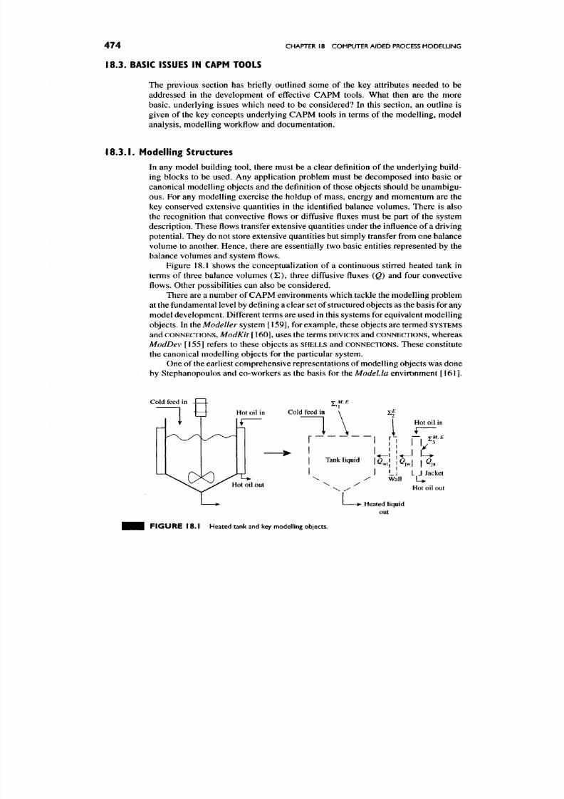
8/17/2019 Process Modelling and Model Analysis-Hangos-Cameron
http://slidepdf.com/reader/full/process-modelling-and-model-analysis-hangos-cameron 491/560

8/17/2019 Process Modelling and Model Analysis-Hangos-Cameron
http://slidepdf.com/reader/full/process-modelling-and-model-analysis-hangos-cameron 492/560
BASIC
ISSUES
IN CAPM TOOLS
475
FIGURE 18*2 Principal modelling objects in a CAPM environment.
Other work has been do ne by Marquardt [160] as the basis for the V E D A and VDD L
language development within
ModKit.
A particular representation of the key objects
in process modelling is seen in Fig. 18.2 as developed by Williams et al. [162]. This
shows the key modelling objects, their interrelationships and their attributes as the
basis for an object oriented model building environment implemented in Java.
18.3.2. Structural Characterization
It is not only necessary for CAPM tools to define principal mo delling objects but those
objects must also be characterized by giving their specific properties or attributes.
It is important that the prop erties of balance v olume s, flow s and fluxes are specified.
CA PM tools must provide facilities for the user to define such properties to produce a
specific instance of a general class of modelling o bject. These class specific attributes
must be defined clearly within the modelling system.
Figure 18.3 shows a dialogue box within the ModDev system which helps char
acterize the behaviour of a balance volume ("shell") used to represent a liquid phase
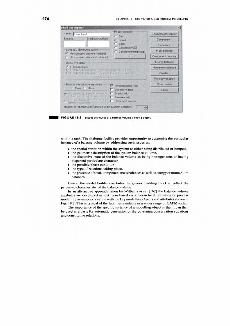
8/17/2019 Process Modelling and Model Analysis-Hangos-Cameron
http://slidepdf.com/reader/full/process-modelling-and-model-analysis-hangos-cameron 493/560
476
CHAPTER 18 COMPUTER AIDED PROCESS MOD ELLING
Shel l descript ion
^^«^'
JTank liquid
Slream^; Shell c^nngc^lonj^:
I C HIcfoscwcbs^anc^fdlslflbMtedj
p Fha$« ecmc^on i
r Sa$ 1
r Cak^Jaltf^q
1
r* Cafe«ls ft{fi(iui'#ta$e) j
EquiifcnufTT 1 |
r Dr^hrrbuted par^icuiated p ro p e rf e fmome nl baianc??
r D sa lfibuled pa ^fe ixs ied p.\ ope?«&^ (p tpi ali cn
?
bafarroe|
•8a«kerthel»^««|uatk«s—1 F imoBp«s«iMefluid
p Sub^titula equ a% ^ of con^^mdlf P* Sravljf field
h Ihs balance Bqmlbm p pfe$^^ f ld
P Use .ub tentid derivativ^ : in te p Q ^ ^ ^ ^ ^ ^ ^
b»sl nce eauafions
Hmhm
dff ip^j l lom{01<fefbe d Inl l«>
pidbkm
dsWioiiJ p ' ^
Oe^^nt^rb descripHon j
Compomi^t
8«ac8or*$
N f ^ $ b ^ ^ i c e
MteMMll)MHiMM(kMMkMlkl(MMlliiMMj
Nommiumb^dnce
Vadal^e^
O l h ^
modeb
Pa^
F I G U R E 18.3 Setting attributes of a balance volume
("shell")
object.
within
a
tank. The dialogue facility provides op portunity to custom ize the particular
instance
of
a balance volume by addressing such issues as:
• the spatial variation within the system as either being distributed or lum ped,
• the geom etric description of the system balance volume,
• the dispersive state of the balance volume as being h omogeneous or having
dispersed particulate character,
• the possible phase condition,
• the type of reactions taking place,
• the presence of total, comp onent mass balances as well as energy or mom entum
balances.
Hence, the model builder can tailor the generic building block to reflect the
perceived characteristic
of
the b alance volume.
In an alternative approach taken by W illiams et
al.
[162] the balance volume
attributes
are
developed
in
text form based
on a
hierarchical definition
of
process
mod elling assum ptions in line with the key modelling objects and attributes shown in
Fig. 18.2. This
is
typical
of
the facilities available in
a
wider range of CAPM tools.
The importance
of
the specific instance
of
a modelling object
is
that
it
can then
be used as
a
basis
for
automatic generation
of
the governing conservation equations
and constitutive relations.

8/17/2019 Process Modelling and Model Analysis-Hangos-Cameron
http://slidepdf.com/reader/full/process-modelling-and-model-analysis-hangos-cameron 494/560
BASIC ISSUES IN C APM TOO LS
477
18.3.3. Multi-level Modelling Hierarchies
One of the important aspects of computer aided modelling is the need for model
representation on various levels of granularity. This could be at the overall flowsh eet
level, unit level or equipment level. The general idea is seen in Fig. 18.4, which
shows a particular hierarchy of model representation. In this figure, we see system
decom position from the flowsh eet level down to the reactor bed level, and agg regation
in the opposite direction. The decomposition could continue down to the individual
catalyst pellet level, where the fundamental behaviour cou ld be described in terms of
a distributed parameter model. These low level building blocks provide the basis for
the modeller to aggregate the lower level systems up to the point of analysis needed
for the application. Th e ability to reuse the fundamental building blocks in a variety
of ways provides powerful facilities for process modelling.
Of course, this aspect of modelling large-scale systems has been available in
commercial flowsheeting packages for decades. However, in the area of CAPM this
concept allows the user to develop building blocks at much lower levels and then
aggregate them into higher level structures as required. A common petrochemical
example might be the model of a distillation column tray which can be re-used and
aggregated into a model of a distillation column. Many systems incorporate such
multi-level modelling hierarchies. A particular example illustrating this concept is
Process Flowsheet
F I G U R E 18.4 Multi-level modelling hierarchy.

8/17/2019 Process Modelling and Model Analysis-Hangos-Cameron
http://slidepdf.com/reader/full/process-modelling-and-model-analysis-hangos-cameron 495/560
478
CHAPTER 18 COMPUTER AIDED PROCESS MODELLING
FIGURE 18 .5 Hierarchical model development in
ModeUa.
seen in Fig. 18.5, which shows the hierarchical decomposition of a CSTR within
the
M odella
environment. In this case, the left pane shows the overall CSTR m odel
being bu ilt, showing the incident convective flows into and out of the reactor and the
cooling jacket. The right-hand pane shows the extended view of the reactor vessel,
clearly made up of two balance volum es— one for the vessel contents and the other for
the cooling
jacket.
At this level the conductive energy flux between the two principal
balance volumes can be seen and described. Further hierarchical decomposition of
the system is possible.
The aggregation of such fundam ental building blocks from the finest granularity
to the upper levels of the hierarchy can be achieved either through textual means as
done in
gPROMS
or graphically as can be seen in
Modella, ModDev
or
ModKit.
Figure 18.6 shows the hierarchy tree describing the aggregation of the fundamental
buildings blocks of v e s s e l and J a c k e t along with the jacket properties to describe
the CSTR model within M odella as already given in Fig. 18.5.
18.3.4. Multi-scale Modelling Hierarchies
In contrast to the multi-level aspects of computer aided modelling, multi-scale mod
elling refers to the ability to capture within the model varying levels of behaviour
or characteristics. The ability to move seamlessly up and down a multi-scale model
hierarchy is an important area for m odel development. T his ability to develop mod els
on multi-scales often reflects the stage of a project or the intended application of the
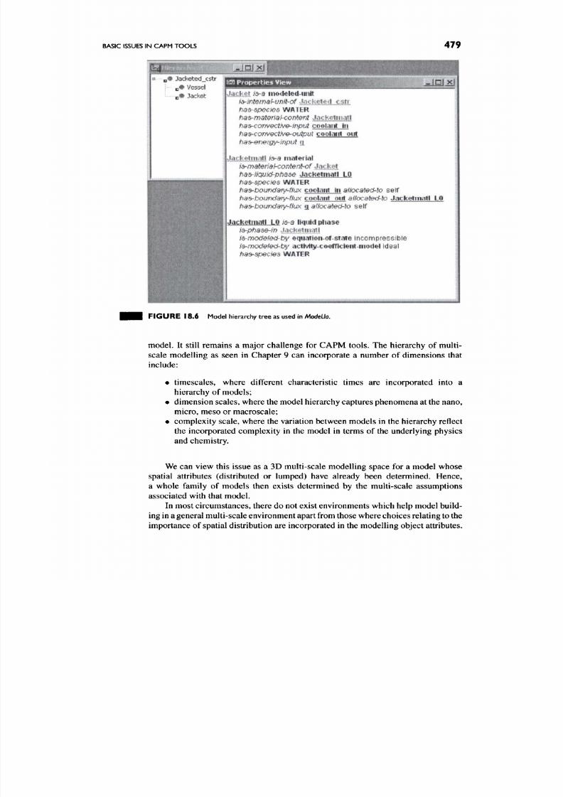
8/17/2019 Process Modelling and Model Analysis-Hangos-Cameron
http://slidepdf.com/reader/full/process-modelling-and-model-analysis-hangos-cameron 496/560
BASIC
ISSUES
IN CAPM TOOLS
479
'',JjQli£l
p# Jacketed_cstr
n» Vessel
n# Jacket
11^
Properties View
W^' '
'js^M
iJacktt \^a mocl^ied-unit
i&-intemaf-unit-of JMb .M# j[ i jr j t l
has-spedes WATER
has-material-content Jack^matl
has-convective-input cookitit in
ha&-convect)ve-oiitput cooiarrt out
has-energ]^input g
Jyiek#tmatl /s-a material
is-materiaf-content-of Jaek i t
has-fiqwd-phase JacketmatJ LP
has-spede WATER
has-boundary-ffux
coolaiit in
aflocatec^to
self
ha&-boitndary-ffitx coolant out afhcated-to Jacketmatl LP
has-boundary-ffux a affocatad-to self
JacketniatI LP js-d liquid phase
ia-phase-in Jack^tt i i^ l
ia-modefed-ty equation-of-state Incompressible
is-modefed-by acttvfty-coefTicient-model Ideal
ha&spedes WATER
FIGURE 18 .6 Model hierarchy tree as used in ModeUa.
model. It still remains a major challenge for CAPM tools. The hierarchy of multi-
scale modelling as seen in Chapter 9 can incorporate a number of dimensions that
include:
• timescales, where different characteristic times are incorporated into a
hierarchy of models;
• dimension scales, where the model hierarchy captures phenomena at the nano,
micro, meso or macroscale;
• com plexity scale, where the variation between m odels in the hierarchy reflect
the incorporated complexity in the model in terms of the underlying physics
and chemistry.
We can view this issue as a 3D multi-scale modelling space for a model whose
spatial attributes (distributed or lumped) have already been determined. Hence,
a whole family of models then exists determined by the multi-scale assumptions
associated with that model.
In most circumstances, there do not exist environments which help model build
ing in a general multi-scale environment apart from those where cho ices relating to the
importance of spatial distribution are incorporated in the modelling object attributes.
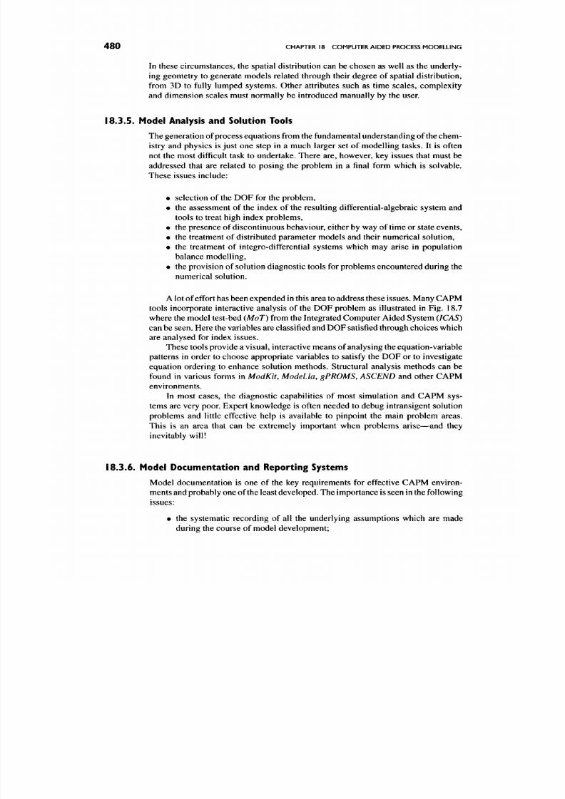
8/17/2019 Process Modelling and Model Analysis-Hangos-Cameron
http://slidepdf.com/reader/full/process-modelling-and-model-analysis-hangos-cameron 497/560
480
CHAPTER
18
COMPUTER AIDED PROCESS MODELLING
In these circumstances, the spatial distribution can be chosen as well as the underly
ing geometry to generate models related through their degree of spatial distribution,
from 3D to fully lumped systems. Other attributes such as time scales, complexity
and dimension scales must normally be introduced manually by the user.
18.3.5. Model Analysis and Solution Tools
The generation of process equations from the fundamental u nderstanding of the chem
istry and physics is just one step in a much larger set of modelling tasks. It is often
not the most difficult task to undertake. T here are, however, key issues that must be
addressed that are related to posing the problem in a final form which is solvable.
These issues include:
• selection of the DO F for the problem,
• the assessment of the index of the resulting differential-algebraic system and
tools to treat high index problems,
• the presence of discontinuous behaviour, either by way of time or state events,
• the treatment of distributed parameter models and their numerical solution,
• the treatment of integro-differential systems which may arise in population
balance modelling,
• the provision of solution diagnostic tools for problems encountered during the
numerical solution.
A lot of effort has been expended in this area to address these issues. Many CAPM
tools incorporate interactive analysis of the DOF problem as illustrated in Fig. 18.7
where the m odel test-bed
(MoT)
from the Integrated Computer Aided System
(ICAS)
can be seen. H ere the variables are classified and DO F satisfied through cho ices which
are analysed for index issues.
These tools provide a visual, interactive means of analysing the equation-variable
patterns in order to choose appropriate variables to satisfy the DO F or to investigate
equation ordering to enhance solution methods. Structural analysis methods can be
found in various forms in ModKit, Model.la, gPRO MS, ASCEND and other CAPM
environments.
In most cases, the diagnostic capabilities of most simulation and CAPM sys
tems are very poor. Expert kn owledge is often needed to debug intransigent so lution
problems and little effective help is available to pinpoint the main problem areas.
This is an area that can be extremely important when problems arise—and they
inevitably will
18.3.6. Model Documentation and Reporting Systems
Model documentation is one of the key requirements for effective CAPM environ
ments and probably one of the least developed. The impo rtance is seen in the following
issues:
• the systematic recording of all the underlying assum ptions which are made
during the course of model development;
8/17/2019 Process Modelling and Model Analysis-Hangos-Cameron
http://slidepdf.com/reader/full/process-modelling-and-model-analysis-hangos-cameron 498/560
BASIC ISSUES IN CAPM TOOLS
481
imrmw.Wmwjmw^rr^^^^ A
F I G U R E 1 8.7 Interactive mod el equation-variable selection system fro m the ICAS m odel test -bed.
• the docum entation of the decisions or reasoning mad e in arriving at a particular
model type;
• the generation of readable mod el descriptions and final reports for comm un
ication and archival purposes.
Inadequacies in the area of documentation can reduce communication of the
modelling effort within organizations, lead to major problems in model re-use or
further development at a later time and create problems of maintainability. A CAPM
system should have self-documen ting c apabilities that are strongly determ ined by the
underlying structure of the objects within the system as well as the tools available to
the user to help document model development. Bogusch
et al.
[160] have suggested
the use of hypertext systems for users to note down decisions made as the modelling
proc eeds. This can be com plemen ted by the use of an issue based information system
(IBIS) [163] which has been used successfully by other workers in engineering design
environments such as Bafiares-Alcantara [164,165]. The IBIS structure consists of
several elements including:
•
Issues:
a statement relating to a modelling problem being faced. This could
be whether a particular energy balance volume such as a reactor vessel wall
should be included or excluded in a model application.
• Positions', a statement setting out the possible positions to be taken and the
preferred position on the issue. In this case it could be to exclude the wall
energy holdup or to include it in the model.
•
Arguments',
statements w hich are used to justify the position taken on resolv
ing the issue. In the case of excluding the wall energy holdup, this might
include such justifications as the wall is thin; that the heat content is small

8/17/2019 Process Modelling and Model Analysis-Hangos-Cameron
http://slidepdf.com/reader/full/process-modelling-and-model-analysis-hangos-cameron 499/560
482
CHAPTER 18 COMPUTER AIDED PROCESS MOD ELLING
Decision
Issue
^"re so l ves i ssue
\ \ \ chosen
\ \
declines \
Position 1
V
supports
Position 2
Position
n
'^k.^pports
Argument 1
^i..-^\'supports
rnnt i^ ryV
supports
Argument m
F I G U R E 18 .8 Typical IBIS structure for decision documentation.
compared with the reactor contents or that, in the time frame considered, the
wall temperature can be regarded as constant.
Key IBIS concepts and their interrelation are shown in Fig. 18.8. The elements
of the decision making can be stored com pactly and retrieved easily by either textual
or graphical means.
18.3.7.
Model Simulation Environments
In many cases, the modelling environment is integrated with a simulation environment
such as in Model, la, which contains its own num erical solution routines. In other cases,
the CAPM tools export final equation systems in a form which can be directly read
into powerful equation solving packages. In the case of
ModKit,
options allow for
the export of models into code readable by gPROMS or SpeedUp. In these cases,
the modelling environment is limited to the model building and generation phases,
numerical solution being done outside the CAPM system.
Wh at is essential is the availability of reliable sim ulation engines that can handle
a range of underlying m odel characteristics. In most cases, current systems are limited
to the solution of index-1 D AE systems. Some systems such as gPROMS and M odel, la
provide a wider range of solution capabilities such as handling the solution of PDEs.
18.3.8. Modelling Decision Support Systems
Decision support systems (DSSs) are commonly used in a range of management
applications. However, little if any use is found in process modelling environments
apart from typical help systems for commerc ial simulators and som e tools in the area
of solvability analysis. DSSs provide timely advice in the most appropriate form on
8/17/2019 Process Modelling and Model Analysis-Hangos-Cameron
http://slidepdf.com/reader/full/process-modelling-and-model-analysis-hangos-cameron 500/560
APPROACHES TO CAPM TOOL DEVELOPMENT 483
which the user can take action. The DSS in no way makes the decision for the user.
DSSs within CA PM tools would help in the following areas:
• guidanc e on the mod elling process and what is required at key steps of the
process;
• advice on the likely implications of making certain modelling assumptions on
the complexity, solvability and model characteristics;
• guidance on w hat is required in the process m odelling in order to meet the
functional specifications for the model;
• advice on selection of DO F and the implications choices have on solvability;
• advice on addressing difficult numerical solution prob lems;
• advice on mod el calibration and subsequent model validation proce dures.
In many cases , DSS tools rely on assessm ent of the current state of the modelling
through analysis techniques and the interpretation of the results. The design of DSSs
is extremely challenging as they must support both novice and advanced users. This
implies analysis and presentation at varying depths of detail.
18.3.9. The Modelling Goal
All mo delling is goal oriented. M odels are built for a particular end-use and not to fill
in idle time of the mod eller In Chapter 1, we discussed the wide ranging app lication
of models in PSE. It is certain that one model does not fit all uses, be it for control,
design or safety studies. It is also imperative that as far as possible the model bu ilder
has a clear modelling specification to work with in developing the m odel. In this case,
it is certain that general specifications can be set down at the outset of modelling w ith
the specification assuming more detail as the modelling and testing proceeds. The
challenge in this issue is to provide guidance to model builders as to the appropriate
choices required throughout the modelling tasks with regard to model characteristics,
form and fidelity.
The area of clearly stating modelling goals and using these in terms of model
building is some times implicitly assumed by expert modellers and completely forgot
ten by novices. No existing CAP M tools appear to address this issue in any structured
way and certainly not
in
any depth. It remains
a
major cha llenge for the next generation
of CAPM tools ... or the generation after that
18.4. APPROACHES TO CAPM TOOL DEVELOPMENT
In this section, we discuss more fully the types of tools which have been developed
or are under development to tackle computer aided process modelling. Some systems
have already been used to illustrate particular aspects of CA PM requirem ents. C urrent
CAPM tools fall into a number of categories although some cross several categories
simultaneously. Various general categorizations have been done by Marquardt [154]
and Jensen [155].
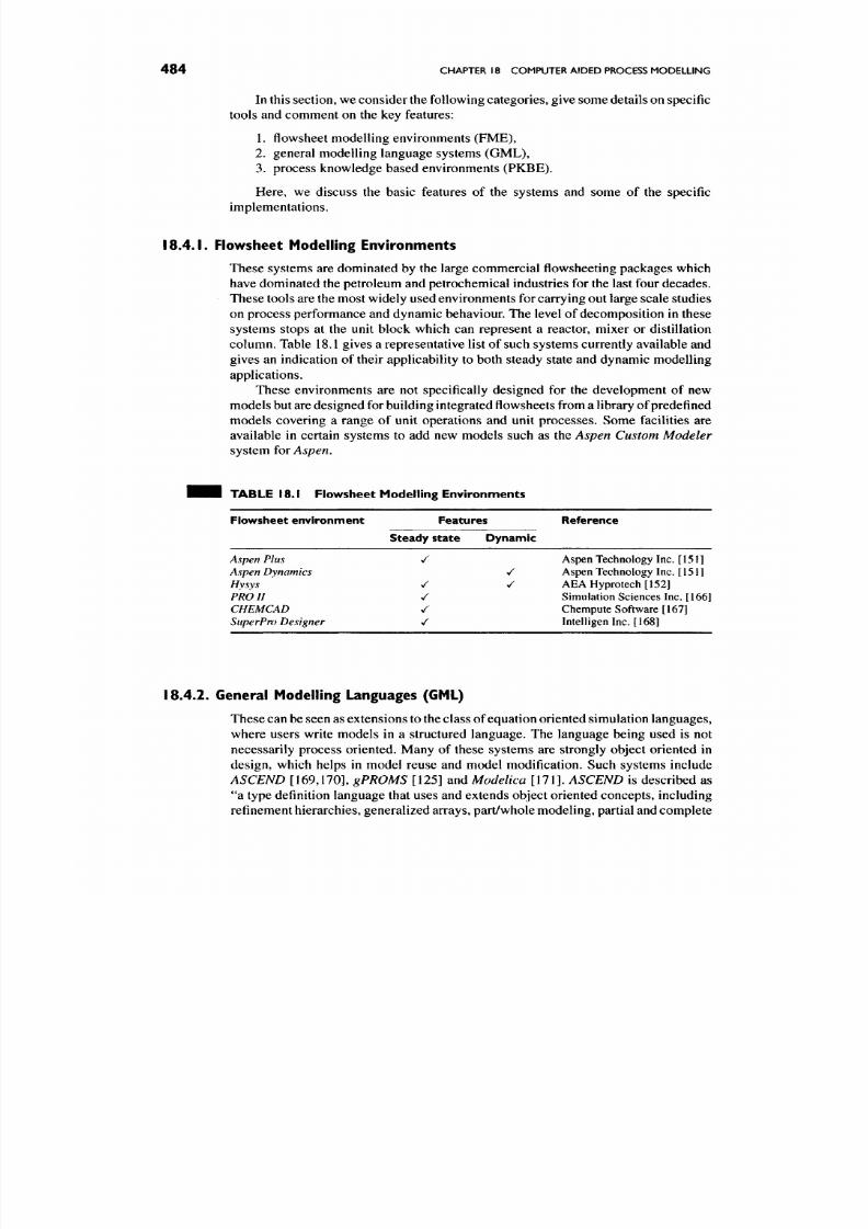
8/17/2019 Process Modelling and Model Analysis-Hangos-Cameron
http://slidepdf.com/reader/full/process-modelling-and-model-analysis-hangos-cameron 501/560
4 8 4 CHAPTER 18 COMPUTER AIDE D PROCESS MO DELL ING
In this section, we consider the following categories, give some details on specific
tools and comment on the key features:
1. flowsheet modelling environments (FM E),
2.
general modelling language systems (GML),
3. process knowledge based environments (PKBE).
Here, we discuss the basic features of the systems and some of the specific
implementations.
18.4.1. Flowsheet Modelling Environments
These systems are dominated by the large commercial flowsheeting packages which
have dominated the petroleum and petrochemical industries for the last four decad es.
These tools are the most widely used environmen ts for carrying out large scale studies
on process performance and dynamic behaviour. The level of decom position in these
systems stops at the unit block which can represent a reactor, mixer or distillation
colum n. Table 18.1 gives a representative list of such systems currently available and
gives an indication of their applicability to both steady state and dynamic modelling
applications.
These environments are not specifically designed for the development of new
mod els but are designed for building integrated flowshee ts from a library of predefined
models covering a range of unit operations and unit processes. Some facilities are
available in certain systems to add new models such as the Aspen C ustom M odeler
system for
Aspen.
TA BL E 18.1 Flowsheet Mod el l ing Environ men ts
Flowsheet environm ent Features Reference
Aspen Plus
Aspen Dynamics
Hysys
PRO I
CHEMCAD
SuperPro Designer
18.4.2. General Modelling Languages (GML)
These can be seen as extensions to the class of equation oriented simulation languages,
where users write models in a structured language. The language being used is not
necessarily process oriented. Many of these systems are strongly object oriented in
design, which helps in model reuse and model modification. Such systems include
ASCEND [169,170], gPROMS [125] and Modelica [171]. ASCEND is described as
"a type definition language that uses and extends object oriented con cepts, including
refinement h ierarchies, generalized arrays, part/whole mod eling, partial and comp lete
Steady state
/
/
^
/
/
Dynamic
/
/
Aspen Technology Inc. [151]
Aspen Technology Inc. [151]
AEA Hyprotech [152]
Simulation Sciences Inc. [166]
Chempute Software [167]
Intelligenlnc. [168]

8/17/2019 Process Modelling and Model Analysis-Hangos-Cameron
http://slidepdf.com/reader/full/process-modelling-and-model-analysis-hangos-cameron 502/560
APPROACHES TO CAPM TOOL DEVELOPMENT
485
T A B L E 1 8 .2 G e n e r a l M o d e l l i n g L a n g u a g e s
G M L
s y s t e m
gPROMS
ASCEND
ModeUca
S t e a d y s t a t e
F e a t u r e s
D y n a m i c D i s t r i b u t e d
Hybr id
/
R e f e r e n c e
P S E L t d [ 1 2 5 ]
Carnegie Mellon [170]
Mode l ica [171]
merging , deferred binding and universal type s" [169]. Table
18.2
gives details of some
of the available systems and their capabilities.
The concepts within these languages reinforce the non-specific domain of the
modelling system. The modelling tools which utilize GML are applicable to a wide
range of application areas. They simply provide a mechanism to develop individ
ual models, link them where necessary and obtain simulated solutions. Process
engineering concepts are developed within these systems from the use of more
generic objects.
Underlying these GML systems are the specific building blocks which are used
to develop the user application. These are not necessarily in the form of modelling
objects as discussed in Section 18.3.1 but are language objects suitable for writing
equations. In the case of ASCEND, the fundamental buildin g bloc ks con sist of ATOMS
and
MODELS,
whereas gPROMS utilizes VARIABLES and
MODELS.
Figure 18.9 shows
the generic building block s for both
ASCEND
and
gPROMS.
A ll ATOMS are inherited
from other ATOMS or from base types such as integer, boolean, real or string. MODELS
are defined in terms of keywords, model variables and equation definitions.
r
ASCEND
Generic Building
Blocks
ATOM
FIGURE 18.9
G e
1
MODEL
neric bi ilding block s in
C
r
gPROMS
Generic Building
Blocks
VARIABLE
.MLs.
1
MODEL
The app lication of the generic mo delling objects is seen in the following example
using the language constructs found in
ASCEND.
EXAMPLE 18.4.1 (Use of these building blocks within AS CE ND ). This is seen
in the following ATOM:
ATOM VariableType REFINES BaseClassName
DIMENSION measure unit dimension
DEFAULT value {measure unit}
lowerJDOund = value {measure unit}
nominal := value {measure unit}
upperJoound := value {measure}
END VariableType
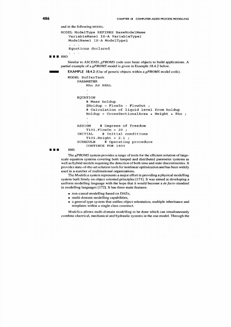
8/17/2019 Process Modelling and Model Analysis-Hangos-Cameron
http://slidepdf.com/reader/full/process-modelling-and-model-analysis-hangos-cameron 503/560
486
CHAPTER
18
COMPUTER AIDED PROCESS MODEL LING
and in the following MODEL:
MODEL ModelType REFINES BaseModelName
VariableNamel IS-A VariableTypel
ModelNamel IS-A ModelTypel
Equations declared
• • • END
Similar to
ASCEND, gPROMS
code uses basic objects to build applications. A
partial example of a gPROMS model is given in Example 18.4.2 below.
• • • EXAMPLE 18.4.2 (Use of generic objects within a
gPROMS
m odel code).
MODEL BufferTank
PARAMETER
Rho AS REAL
EQUATION
# Mass holdup
$Holdup = Flowin - FlowOut ;
# Calculation of liquid level from holdup
Holdup = CrossSectionalArea * Height * Rho
ASSIGN # Degrees of freedom
TlOl.Flowin = 20 ;
INITIAL # Initial conditions
TlOl.Height = 2.1 ;
SCHEDULE # Operating procedure
CONTINUE FOR 1800
END
Th e gPROMS system provides a range of tools for the efficient solution of large-
scale equation systems covering both lumped and distributed parameter systems as
well as hybrid mo dels requiring the detection of both time and state discontinuities. It
provides state-of-the-art solution tools for nonlinear optimization and has been widely
used in a number of multinational organizations.
Th e
M odelica
system represents a major effort in providing a physical modelling
system built firmly on object oriented principles [171]. It was aimed at developing a
uniform modelling language with the hope that it would become a
de facto
standard
in modelling languages [172]. It has three main features:
• non-causal modelling based on DA Es,
• multi-domain modelling capabilities,
• a general type system that unifies object orientation, multiple inheritance and
templates within a single class construct.
Modelica
allows multi-domain modelling to be done which can simultaneously
combine electrical, mechanical and hydraulic systems in the one model. Through the

8/17/2019 Process Modelling and Model Analysis-Hangos-Cameron
http://slidepdf.com/reader/full/process-modelling-and-model-analysis-hangos-cameron 504/560
APPROACHES TO CAPM TOOL DEVELOPMENT 487
use of a Graphical User Interface (GUI), the system allows compositional modelling
to be done using high level descriptions of the objects through the use of building
block icons. The facilities of Modelica, are extended by the design environment
MathModelica which provides a Mathematica-like notebook capability providing
documentation of:
• parts of models,
• text or docu men tation,
• dialogue for for specification and modeification of input data,
• results tables,
• graphical result representation,
• diagram s to aid in the visualization of the model structure.
Modelica m odels generated by the system can be solved in the simulation system
Dymola or can be generated as C++ code for direct execution.
General mo delling languages pro vide powerful features to address general prob
lems which are not restricted solely to process systems. They can be equally applicable
for developing large-scale national economic models as they are for developing pro
cess specific m odels. They rely heavily on the user developing and coding directly all
equations and variables associated with the application. These GML systems have a
long established history within PSE and are widely used by the engineering commu
nity. New systems such as ABACUSSII also address the general modelling area with
features for hybrid modelling
[173].
18.4.3. Process Knowledge Based Environments (PKBE)
In contrast to GML systems, process modelling languages (PMLs) are specifically
designed for the application area of process engineering. Fisher et al. [174] point
out that in order to improve utility and enhance usefulness, a modelling tool should
not add complexity to the task but simplify it. Providing a user with a language
directly related to the problem domain should make the process of modelling more
transparent. M ost of these PM Ls are embedded w ithin a larger mod elling environment
which typically uses a GUI to build the model from the key building blocks. These
systems we can denote as process knowledge based environments. In these cases, the
modelling language is used to describe the model in process engineering terms and
as such is required to be flexible enough to encompass all possible process modelling
situations. In most cases the user sees the m odel description in the language but does
not necessarily write directly in that language. Tools such as
Mod el, la
[161,175],
ModDev [155] and Modeller [159] belong to this class. Facilities are often available
to post-edit the equation system which is generated in the chosen PKBE.
The use of domain specific concepts also makes the transition from a text based
interface to a graphical interface muc h simpler as icons can replace meta-w ords. This
can be seen for example, in the user interfaces
of Model.la
and also
ModKit
shown
in Figs. 18.11 and 18.12.
ModeUa Environment
In the case
of Model.la
the interaction (Fig. 18.11) takes place through a GUI which
provides access to all the construction and analysis tools. Icons within the Modeling
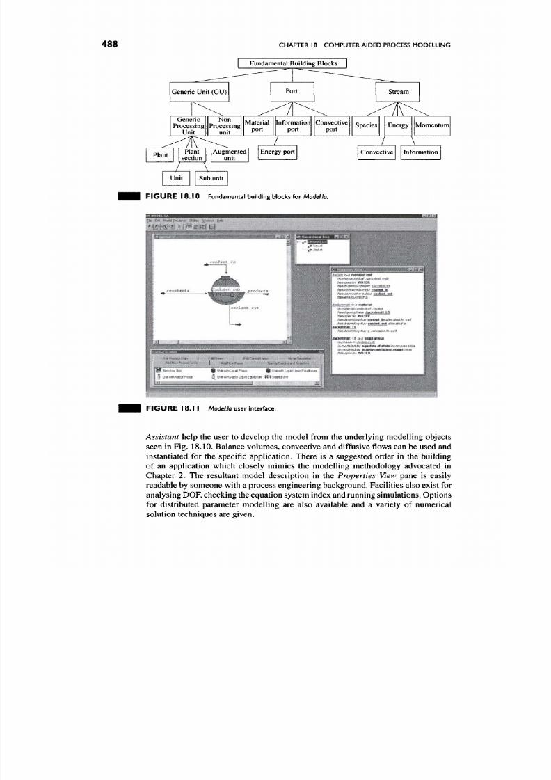
8/17/2019 Process Modelling and Model Analysis-Hangos-Cameron
http://slidepdf.com/reader/full/process-modelling-and-model-analysis-hangos-cameron 505/560
488
CHAPTER 18 COMPUTER AIDED PROCESS MOD ELLING
F I G U R E 18 .1 0 Fundamental building blocks for
ModeUa.
^ ^ }
w^
roactsnts
oolant out
^ ^
WBIackbcwUn*
I d UmtwilhVapM Phase
Unt wlh Liqud Phase j | | Unit with LiquK) Liqud Equtbu m
||^ Un» with Vapoi Liquid E quftrium M I Staged Unit
, ^ -:J U
j i i i i i l l i i M i i i M
F I G U R E
18.
I I
Modeiia
user interface.
Assistant
help the user to develop the model from the underlying modelling objects
seen in Fig. 18.10. Balance volume s, convective and diffusive flows can be used and
instantiated for the specific application. There is a suggested order in the building
of an application which closely mimics the modelling methodology advocated in
Chapter 2. The resultant model description in the Properties View pane is easily
readable by someone with a process engineering background. Facilities also exist for
analysing DOF, checking the equation system index and running simu lations. Options
for distributed parameter modelling are also available and a variety of numerical
solution techniques are given.

8/17/2019 Process Modelling and Model Analysis-Hangos-Cameron
http://slidepdf.com/reader/full/process-modelling-and-model-analysis-hangos-cameron 506/560
APPROACHES TO CAPM TOOL DEVELOPMENT
489
r:«sa Ca^s jxa Pajswe f / fc j ia iscJs
Chjr*ji. tSeiLS
F I G U R E 1 8 .1 2
ModKit
user interface.
ModKIt Environment
The
ModKit
system is an advanced process modelling tool built upon a well-defined
object oriented data model V E D A which utilizes a formal process engineering repre
sentation language VDDL ( V E D A data definition language). It is a development of
the process systems group at the Lehrstuhl fiir Prozesstechnik at Aachen University
of Technology. Figure 18.12 shows a typical GUI for the system which is built upon
the
G2
expert system software from Gensym Corporation [176].
The GUI displays some of the key aspects of the interactivity available in the
system including the model building pane at the top right where the fundamental
building blocks are assembled. As well, the attributes of a specific modelling object
can be selected and set through interactive windows. In this case the lower right pane
shows the attributes assoc iated w ith a flash unit which is part of the overall flowsheet.
Equations and variables can also be accessed for particular sections or models of the
flowsheet under construction.
ModKit
provides features for model documentation through its IBIS system sup
plemented by hypernotes which are attached to the IBIS structure. Other facilities
include the ability to analyse the equations for DO F and index, and gen erate the code
suitable for simulation within
SpeedUp
or
gPROMS.
The system embodies most of the attributes of a fully functional process
modelling tool and continues to undergo refinement and expansion.
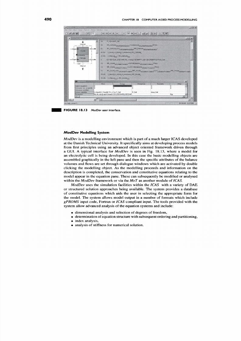
8/17/2019 Process Modelling and Model Analysis-Hangos-Cameron
http://slidepdf.com/reader/full/process-modelling-and-model-analysis-hangos-cameron 507/560
490
CHAPTER 18 COMPUTER AIDED PROCESS MODE LLING
,i-Ai'ririttt^iik;.>>V^B.rih<A<»»^^^^
f_Afeed(il f_Cfeed[il TN_rr Cut T„Cel
|N C Hr ne(m l ne[mSulfa(eO CEO^CECOMPti) CECOMP
0
P_Ce«
-f*L.
•M\
ft^m^fififmn
r ^
'"Wi^^^MWA
F I G U R E 18 .13 AlodDev user interface.
/^odDev Modelling System
ModDev is a modelling environment which is part of a much larger ICAS developed
at the Danish Technical U niversity. It specifically aims at developing process mod els
from first principles using an advanced object oriented framework driven through
a GUI. A typical interface for ModDev is seen in Fig.
18.13,
where a model for
an electrolytic cell is being developed. In this case the basic modelling objects are
assembled graphically in the left pane and then the specific attributes of the balance
volumes and flows are set through dialogue windows which are activated by double
clicking the modelling object. As the modelling proceeds and information on the
description is completed, the conservation and constitutive equations relating to the
model appear in the equation pane. These can subsequently be modified or analysed
within the ModDev framework or via the M oT as another module of/CA5.
ModDev
uses the simulation facilities within the
ICAS
with a variety of DAE
or structured solution approaches being available. The system provides a database
of constitutive equations which aids the user in selecting the appropriate form for
the model. The system allows model output in a number of formats which include
gPROMS input code, Fortran or ICAS compliant input. The tools provided with the
system allow advanced analysis of the equation systems and include:
• dimensional analysis and selection of degrees of freedom,
• determination of equation structure with subsequent ordering and partitioning,
• index analysis,
• analys is of stiffness for num erical solution.
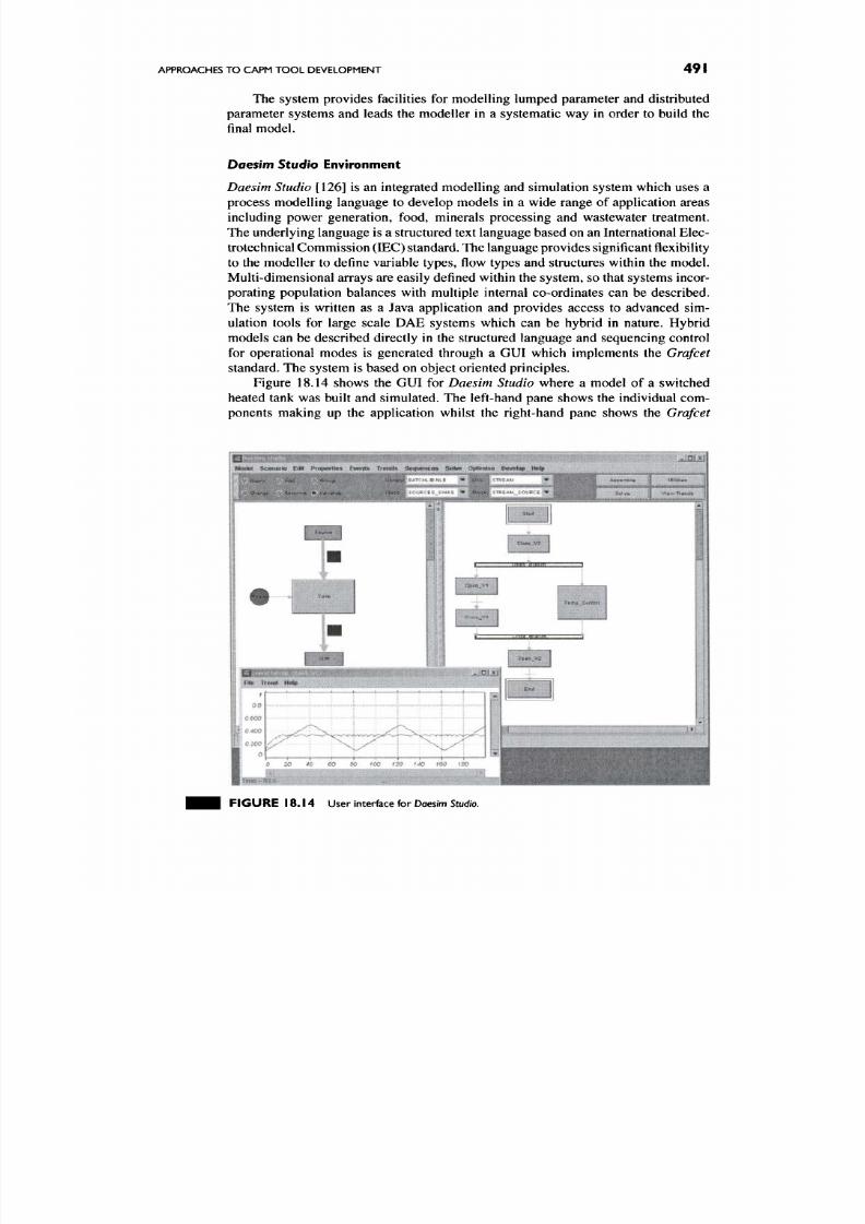
8/17/2019 Process Modelling and Model Analysis-Hangos-Cameron
http://slidepdf.com/reader/full/process-modelling-and-model-analysis-hangos-cameron 508/560
APPROACHES TO CAPM TOOL DEVELOPMENT
491
The system provides facilities for modelling lumped parameter and distributed
parameter systems and leads the modeller in a systematic way in order to build the
final model.
Daesim Studio Environment
Daesim Studio [126] is an integrated modelling and simulation system which uses a
process modelling language to develop models in a wide range of application areas
including power generation, food, minerals processing and wastewater treatment.
The underlying language is a structured text language based on an International Elec-
trotechnical Com mission (DEC) standard. T he languag e provides significant flexibility
to the modeller to define variable types, flow types and structures within the model.
Multi-dimensional arrays are easily defined within the system, so that systems incor
porating population balances with multiple internal co-ordinates can be described.
The system is written as a Java application and provides access to advanced sim
ulation tools for large scale DAE systems which can be hybrid in nature. Hybrid
models can be described directly in the structured language and sequencing control
for operational modes is generated through a GUI which implements the
Grafcet
standard. The system is based on object oriented principles.
Figure 18.14 shows the GUI for Daesim Studio where a model of a switched
heated tank was built and simulated. The left-hand pane shows the individual com
ponents making up the application whilst the right-hand pane shows the
Grafcet
^'Um
« » « H . J «
6 f e i * < «
.'t*wph^6««Bw» i
FIGURE 18 .14 User interface fo r Does/m Stud/0.
8/17/2019 Process Modelling and Model Analysis-Hangos-Cameron
http://slidepdf.com/reader/full/process-modelling-and-model-analysis-hangos-cameron 509/560
492
CHAPTER
18
COMPUTER AIDED PROCESS MODEL LING
diagram for the sequenced control of the heater. Simu lated behaviour is shown in the
results pane.
Daesim Studio provides facilities for managing model libraries which are main
tained in classes and members. The structured text language provides advanced logic
within the model description allowing the development of hybrid models. Simulation
facilities are supported by large scale DAE solvers which handle both index-1 and
index-2 systems that can be conventional or hybrid in character. Model libraries of
modelling primitives can be developed and then used to assemble complex models
consisting of these building blocks.
These previous sketches of CAPM tools have given some idea of the types of
systems now being developed w hich are capable of tackling process mo delling appli
cations. M ost of them share com mon ideas in their construction and there is a growing
number of the tools available. Some like
ModKit
or
ModDev
are designed to gener
ate output compatible with well known simulation systems. Others such as M odelJa
and
Daesim Studio
provide both modelling and simulation environments in the one
environment.
It is clear that these tools will continue to grow in importance as process sys
tems engineers demand more advanced tools to carry out modelling of new and
non-traditional processes not covered by commercial flowsheet simulators.
18.5.
SUMMARY
CAPM is an extremely important area of modelling practice. Conventional simula
tion tools provide some ability to develop new models or modify existing models.
However, CA PM tools that specifically address the issue of model b uilding are vital
for better uptake of mo delling in the process industries. It has been seen that several
approaches are possible in developing these tools. Some work at the level of writing
equations whilst others work at a much higher conceptual level, where most users
would naturally work.
It is likely that the approaches which work at the physical description level dealing
with balance volumes, flows and fluxes will become increasingly important. This is
where most engineers and scientist naturally think about the systems they wish to
model. New developments in structured assumption hierarchies [177] could play an
increasingly important role in model development and self-documentation of mo dels.
Other work on model hierarchies and the ability to develop families of models with
different complexity, time or dimension scales for different applications will play an
important future role in CA PM
tools.
Finally, developm ents to try and guide m odellers
based on the intended end-use of models will be important in encouraging uptake of
these techniques in the process indu stries. Efficient model developm ent is an incentive
for the increased use of process models in a wide range of applications and industry
sectors.

8/17/2019 Process Modelling and Model Analysis-Hangos-Cameron
http://slidepdf.com/reader/full/process-modelling-and-model-analysis-hangos-cameron 510/560
EMPIRICAL MODEL BUILDING
l9.I.INTRODUCTrON
Process modelling is an iterative and incremental engineering activity. Theoretically,
well-grounded elements based on first engineering principles and empirical parts
based on measured data, operational experience and engineering heuristics or any
combination of these are present in most models. In a realistic process modelling
activity there is almost always a need for empirical m odel building . This is the subject
of this chapter.
The purely empirical model elements are called black-box elements in contrast
to the white-box elements based on first engineering principles. It is important to re
cognize, however, that process models are always grey-box models in nature. That is,
they contain both black and white parts. Therefore, empirical or black-box mod elling
is treated in the context of grey-box modelling.
The material in the chapter is presented in the following sections:
• First the SEVEN STEP MODELLING PROCEDURE introduced in Section 2.3 is
revisited in Section 19.2 to examine the need for empirical mo delling and the
problems which may arise during this procedure calling for an empirical or
black-box model element.
• Thereafter, the most popular and most widely used black-box model struc
tures are presented in Section 19.3 together w ith the relationship of black-bo x
modelling to model calibration and identification.
• Finally, the most comm on traps and pitfalls in empirical mod el building are
described in Section 19.4 along with methods to detect and deal with them.
493
8/17/2019 Process Modelling and Model Analysis-Hangos-Cameron
http://slidepdf.com/reader/full/process-modelling-and-model-analysis-hangos-cameron 511/560
494
CHAPTER
19
EMPIRICAL MODEL BUILDING
19.2.
THE MODELLING PROCEDURE REVISITED
In Section 2.3 of Chapter 2 a systematic SEVEN STEP MODELLING PROCEDURE is
described which gives a solid framework for the model b uilding process. The iterative
nature of the modelling is also emphasized. It means that we may need to step back
to an earlier modelling step in the procedure if the results of a later step are not
satisfactory.
19.2.1.
Grey-box Models: Models with Black-box Elements
The notion of grey-box models has been introduced as early as Chapter 2 these
being models with both white (purely mechanistic) and black (purely empirical)
model elements. Thereafter, in Section 12.1 of Chapter 12 on Grey-Box Models and
Model Calibration, grey-box m odels were defined as process models developed using
first engineering principles but with part of their model parameters and/or structure
unknow n. From this understanding and description we can infer what kind of elements
in a process model may be black-box types.
If one follows the systematic SEVEN STEP MODELLING PROCEDURE then the
ingredients of a mathematical model developed using first engineering principles
will always be as follows:
• balance volumes,
• balance equations being (ordinary or partial) differential eq uations,
• constitutive equations which are algebraic equation s,
• initial and boundary conditions.
The classification and properties of the terms in balance equations, as well as
the main categories of constitutive equations and their properties fixes some addi
tional mathematical properties, like the possible type of the PDEs derived as balance
equations.
It follows from the above that the black-box model elements in a process model
should also fall into the categories above and respect the properties of the category they
belong to. It is also clear that black-box elemen ts may have very different comp lexity
ranging from simple parameters up to balance equations being PDEs with partially
unknown structure. This view on grey-box models is much broader than that used in
Section 12.1 where the unknown parameter case was only considered in most of the
cases.
19.2.2.
Steps Calling for Black-box Elements
The mathem atical model of a process system is developed in steps 1-4 of the
SEVEN
STEP MODELLING PROCEDURE where we return from later steps if we want to refine
the model. In carrying out these steps, various circumstances may indicate the need
for empirical or black-box model elements as follows:
2. Identify control mechanisms
When recognizing controlling mechanisms important for the modelling prob
lem, we may find rather unusual or poorly understood mechanisms, such
as biomass degradation, for example, together with relatively well-described
8/17/2019 Process Modelling and Model Analysis-Hangos-Cameron
http://slidepdf.com/reader/full/process-modelling-and-model-analysis-hangos-cameron 512/560
THE MODELLING PROCEDURE REVISITED
495
ones, like evaporation, heat and mass transfer, etc. Such a poorly understood
or less investigated controlling mechanism will call for a black-box model of
its own if any measured data is available.
3.
Evaluate the data for the problem
When e ncoun tering the data needed for
the
mod el we may find out that some of
the model param eters, for example reaction kinetic constants, are not available
in the literature. Then we have to find alternative ways to obtain or estimate
them, most often by using measured data. For this purpose, we may use either
the whole original model or just a special part of it or some other model built
for the estimation purpose.
4.
Develop the set of model equations
In formulating the model in step 4 it may turn out that we cannot get data for
the model form we arrived at. This w ill result in a grey-box model where either
the parameters or some of the model elements are unknown. We can either
use model calibration to get the missing parameters using measured data or
look for additional models which relate available data for the unknown model
element.
The black-box m odel elements that we need to make a process m odel com plete
may be one of the following three main types arranged in their decreasing order of
complexity. The types
are
defined according
to the
mathem atical form of the black-box
model element and its role in the overall model.
m :
model-type
The most complex case is when it is a lack of a description of a mechanism based
on first engineering principles. This means that there is an unknown (or partially
known) mechanism, for example fermentation, present in our model. Therefore, the
corresponding constitutive equations, terms in balanc e equations or com plete balances
are missing from the overall model.
The mathematical form of the black-box model element of this type is usually
an explicit nonlinear algebraic equation or a differential equation which is first order
in the time derivative.
The following simple example shows a grey-box model containing a black-box
element of this type.
• • • EXAMPLE 19.2.1 (A simple continuous stirred fermentor).
Problem statement
A perfectly stirred continuous fermenter produces alcohol from sugar. A solution of
sugar in water is fed to the fermenter, where the bioma ss is already present. The outlet
does not contain anything from the biomass but contains water, produced alcohol
and remaining sugar. Describe the dynamic behaviour of the fermenter for control
purposes.
Modelling assumptions
Al. Perfect mixin g.
A2.
Cons tant liquid volum e.
A3.
Isothermal conditions.
A4. Inlet contains only water and sugar.
^ 5 . The fermentation prod uces alcohol from sugar.
8/17/2019 Process Modelling and Model Analysis-Hangos-Cameron
http://slidepdf.com/reader/full/process-modelling-and-model-analysis-hangos-cameron 513/560
496
CHAPTER
19
EMPIRICAL MODEL BUILDING
A6,
Constant physico-chem ical prope rties.
Al. Open-air tank with constant pressu re.
Balance equations
Sugar mass balance
dt
-^ = ^4 -
- S
- ra tes (^s ,^ B,M ), (19.1)
Alcohol mass balance
dx\
V— - = -vxA + rates(xs, XB, XA), (19.2)
Overall biomass mass balance
dxn
V - - f = r a t e B ( ^ S , - ^ .M ) , (1 9.3 )
at
where
V
is the volume of the liquid in the fermenter,
x s,
XB and JCA is the conc entration
of the sugar, biomass and alcohol respectively, and v is the volumetric flowrate.
The fermentation mechanism is largely unknown which affects the component
mass balances and the reaction rate expressions. In the equations above, we can
identify the following black -box elem ents calling for emp irical modelling.
1. The reac tion rate expressions ra tes (- S»- B. ^ A ) and rate A (^S » - B , -^A) and their
relationship. This is a function type black-box element.
2. The overall biomass mass balance equation (19.3). If the required accuracy
dictated by our modelling goal requires modelling the fermentation kinetics
in more detail, then we need to construct more balances for the various kinds
of bacteria in the biomass. This would call for a set of additional balance
equations and then this is a model-type black-box element of our model.
f: function-type
If there is no structure and/or param eters available for a constitutive equation (func
tional relationship), then a function-type black-box model is to be constructed. This
black-box model element is an algebraic equation in its mathematical form which
may be im plicit and is usually nonlinear.
0 =fyi(x\, . . .,
Xn;
Jl , . . ., ym). (19.4)
where Xj is a differential variable,
yi
is an algebraic variable and^. is an unknown
but deterministic function.
Examples of this type of black-box model element are usually rate equations,
such as reaction or transfer rate equations . This is the case in Example 19.2.1 above
where the fermentation rate expressions rates(j^s, J C B , XA) and rateA(^s» -^B* ^A) and
their relationship was unknown.
p:
parameter-type
A parameter-type black-box element arises when one or more of the parameters in a
process m odel are unknown. T his is the case we can in fact handle: we use m easured
data and model calibration to get an estimate of the missing parameter(s).
As we shall see later in this chapter, parameter-type uncertainty is the one to
which we transform both function-type and model-type uncertainties.

8/17/2019 Process Modelling and Model Analysis-Hangos-Cameron
http://slidepdf.com/reader/full/process-modelling-and-model-analysis-hangos-cameron 514/560
BLACK-BOX MODELLING 497
19.3. BLACK-BOX MODELLING
Black-box elements always appear in connection with white elements.
The
structure of a process mode l is white
which fixes:
1. the number and terms in the balance equations,
2. the functional form of some of the constitutive equation s.
This implies that black-box elements are to be imbedded in a white structure.
Therefore neither the overall model nor its elements are ever completely black, at
least some of their structural properties are known
a priori,
19.3.1. Model Calibration and Black-box Modelling
In Section 12.1 in Chapter 12 on
Model calibration,
we have seen that model cali
bration is essentially estimation of unknown model parameters of a given grey-box
model with only parameters unknown using measured data and a measure of fit.
If not only parameters but functions or complete mechanisms described by bal
ance and/or constitutive equations are missing in a grey-box model, then empirical
or black-box modelling should be applied "to fill the gap". The two cases, however,
are strongly related from model calibration point of view.
As we have already seen in Chapter 12 the MODEL STRUCTURE ESTIMATION
is solved by constructing a set of candidate model structures with unknown para
meters and performing a MODEL PARAMETER ESTIMATION to get a model with best
fit. The same technique is applied when we build an empirical model for a model-
type or function-type black-box model element. As we shall see in the following,
we parametrize the problem by selecting a suitably rich nonlinear black-box model
structure and then estimate its parameters using measured data and a measure of fit.
19.3.2. Sensitivity of Models with respect to their Parameters and Variables
If an empirical model or function type black-box model is to be constructed from
measured data the first thing to find out is the set of independe nt variables and para
meters of the model. Later on, when candidate model structures are constructed, we
may want to verify their set of independent variables and parameters. Sensitivity
calculations are suitable for both purposes.
Sensitivities with respect to model parameters are also used in transferring
uncertainty information about a black-box model when imbedded into its white-box
environment.
In order to discuss the most general case for sensitivity calculations the following
general model structure is used:
dx
— =f(x;p), x(to)=xo. (19.5)
d^
y = 8ix;p),
(19.6)
where x(t) e TZ , y(t) e TV and p € TV^\ Note that the above model is in the form
of a DAE containing both model-type uncertainty in Eq. (19.5) and function-type

8/17/2019 Process Modelling and Model Analysis-Hangos-Cameron
http://slidepdf.com/reader/full/process-modelling-and-model-analysis-hangos-cameron 515/560
498
CHAPTER 19 EMPIRICAL MODEL BUIL DING
uncertainty in Eq. (19.6). Note that the solution [x(t), y{t)], to <
t
isa. function of/?
being the vector of the parameters, that is [x{t; /?), y{t: /?)], ^o
S t.
Parametric Sensitivity
The parametric sensitivity of
a
scalar variable v
=
v(^) with respect to
a
scalar
parameter q is characterized by the derivative
dv
Tq
taken at any reference point
q =
q^.ln the process modelling context, static and
dynamic models relate variables and their sensitivities with respect to the same
parameter.
In the case of dynamic models in the form of (19.5), the parametric sensitivity
(px^p of the dynamic vector variable x with respect to the vector parameter /? is
a
time-dependent matrix with the partial sensitivities as its elements:
djc/
VPx,pit)]ij = T~W'
/ =
1,..., n,
; =
1, .. . , m (19.7)
dpj
taken at a reference point/? = p^.
If we take dpj as a parameter and consider that the total derivative offi(x{p), p)
with respect to
Apj
is
d -
dfi
x dfi Axi
JL==JL^J2^T^ (19.8)
we can obtain the total derivative of both sides of Eqs. (19.5) and (19.6) in the
following form:
;[
^ =
Y.^3f,xM(Px,pi^)]ej
+ ,
l(Px,p]ij{to) = 0, (19.9)
m
[(Py,p(t)]ij
= Y1^3g,^M(pyA0]ej (19.10)
e
with
Jy j^^
and
Jg^x
being the Jacobian matrices of
the
right-hand sides of the equations
with respect to the variable x respectively. Note that all the Jacobian and sensitivity
matrices should be taken at a reference point/? = p^. Finally, the above equations
can be written in the following compact matrix-vector form:
^ ^ ^
= Jf,x(Px,p(t)-\-3f,p,
(Px,pUo)
= 0, (19.11)
(Py.p =3g,x(px,p,
(19.12)
where 5fp is the Jacobian matrix of the right-hand side of
Eq.
(19.5) with respect to
the parameter/? taken at a reference point p = p^.
Note that the sensitivities [(Px,p{t)]ij at any point
t
in time can be calculated by
solving the differential equation (19.9). This can be conveniently performed simul
taneously with the original differential equation (19.5) because the Jacobian matrices
needed are available at any point
t
in time.
8/17/2019 Process Modelling and Model Analysis-Hangos-Cameron
http://slidepdf.com/reader/full/process-modelling-and-model-analysis-hangos-cameron 516/560
BLACK-BOX MODELLING 499
Variable Sensitivity
The sensitivity of a solution [x(t),
y{t)], to <t
of Eqs. (19.5) and (19 .6) at any point
t
with respect to the variables is characterized by the derivatives
dx dv
6x0
djo
where jo = gi^o) with the other parameters fixed. This case can be regarded as a
special case of parametric sensitivity when the right-hand side functions/ and g do
not depend explicidy on the parameters
p = xoorp = yo
respectively.
Therefore, the sensitivity equations (19.11 ) and (19.12) should be solved in order
to calculate the variable sensitivities with
Jfp =
0. It is important to notice that the
sensitivity equations (19.11) and (19.12) contain the Jacobian matrices with respect
to the variable
x .
In this case, the dynamic sensitivity equation (19.11) is the same as
the locally linearized version of Eq. (19.5) taken at a reference point
x = x^.
This
gives the connection between variable sensitivities with model linearization which
was described in Section 10.4.
193.3. Black-box Model Structures
The core of a black-box model is an unknown function to be determined from meas
ured data. This function can be present on the right-hand side of a conservation balance
or in a constitutive equation. T he estimation of a comp letely unknow n function is an
ill-posed problem from a mathematical point of view as we have already seen in the
case of MODEL STRUCTURE ESTIMATION problem statement in Section
12.4.
The way
to make the problem mathematically feasible is to construct the
set ofpossible model
structures for the structure estimation problem and determine the best-fit model from
this set by performing a set of model parameter estimation.
The same technique is applied here for black-box modelling. We usually select a
black-box m odel structure set, which fits to the modelling problem and easy-to-han dle
from the estimation point of view at the same time. The elements in a black-box
model structure set have similar structure, and an element from the set is identified
by its structural indices. There are various well known and popular black-box model
structures which will be briefly described in this section.
The following requirements hold for a good black-box model structure:
• simplicity—in its mathematical form resulting in an easy computation, such
as a power series,
•
generality (descriptive power)
—to ensure that the members of the structure
set can describe all possible black-box models in question,
•
flexibility
— to have a wide descriptive range of the structure set.
The above requirements call for an approximation which is similar to an infinite
functional series expansion.
How to select a suitable black-box m odel class which fits the modelling pro blem?
The application area of the class should match the key characteristics of the problem.
The following key characteristics can be taken into account.
8/17/2019 Process Modelling and Model Analysis-Hangos-Cameron
http://slidepdf.com/reader/full/process-modelling-and-model-analysis-hangos-cameron 517/560
500 CHAPTER 19 EMPIRICAL MODEL BUILDING
1. Type
o f the black-box mod elling problem
A function-type black-box m odelling problem calls for a static model structure
while a model-type problem may require dynamic model structures.
2. Other properties of
the
problem
The following properties—if known in advance—may be taken into account:
• linearity-nonlinearity,
• symmetry,
• time-invariance (constant param eters).
The black-box model classes or model structures are described using the
following items:
• Mathem atical description
The mathem atical form of the general element from the set of black-box m odel
structures are given. This determ ines the descriptive po wer and the flexibility
of the structure set.
• Structural parameters
The model parameters used to select one of the members from the set are
described here together with how to estimate them from measured data.
• Mathem atical properties
The special mathematical properties of the general form as well as the
related parameter and structure estimation are given here. These are in close
relationship with the mathematical form of the structure set.
• Parameter estimation
The parameter estimation methods available for the model class are described
briefly for the parameter set including structural param eters.
Linear Static Model Structures
Mathematical description
This is the simplest case when w e need to develop a black-box model for an unknow n
linear function in the overall model in the form of
N
y = Y^XiPi =
x'^P>
(19.13)
/ = 1
Structural parameters
N and the set of variables present in the vector x •
Parameter estimation
The parameter estimation of linear static model structures is described in Sec
tion 12.3.1. It is important that the problem statement of the parameter estimation
requires a loss function which serves as a measure of fit for the estim ation.
The structural parameters can be estimated along the lines shown by the general
MO DEL STRUCTURE ESTIMATION problem statement in Section
12.2. We
construct the
set of possible model structures
including every possible (A^, x) pair and determine
the best-fit model from this set by performing a set of model parameter estimations.
The following examp le shows the use of linear static mod el structures to construct
function-type black-box models.
8/17/2019 Process Modelling and Model Analysis-Hangos-Cameron
http://slidepdf.com/reader/full/process-modelling-and-model-analysis-hangos-cameron 518/560
BLACK-BOX MODELLING 501
• • • EXAMPLE 19.3.1 (Reaction rate expression ). Let us assum e we have
a
partially
known reaction kinetic expression
r = kQe-^l('' ' '^Cl'Cf
(19.14)
in a grey-box model with the reaction orders QA and q s possibly equal to zero, that is
r
may or may not depend on any of the concentrations.
We need to estimate the
• parameters: ko, E,
• structural parameters: qA^Q B-
First, we transform the reaction rate equation to linear in parameter form by
taking the natural logarithm of both sides:
E
l n r = l n / : o - — H - ^ ^ l n Q + ^ f i l n Q . (19.15)
Thereafter, we can notice that the structural parameters become ordinary parameters
in this case and the following correspondence can be made with Eq. (19.13):
j = ln r, x = [ l . --^^ I n Q , I n Q ] ' ^ , p = [\nkQ, E, qA. qsf-
Kl
Nonlinear Static Model Structures and Artificial Neural Networks
Nonlinear static model structures are used to approximate the general case of static
functional relationship in Eq. (19.4).
Functional Series Approximation
Mathematical description
The simplest one is the Taylor series expansion:
n-\-m n+m
yi = ^0 + X I ' * " I Z ^hii^^h ' Xh
n-\-m
+
• • •
+
J2
^' i -
^ 1 • • • X/;v
+
• • •'
(19.16)
where the vector x contains all the variables including both the differential and
algebraic ones:
X = [ x i . . . x^ y\ ...ymf-
It is important to note that the Taylor series expansion is
linear in its parameters
P = [(Ci,i=
l , . . . ,m
+ /z)
ici^i2,iui2
= 1 , . . . , m +
n ) , . . . ,
8/17/2019 Process Modelling and Model Analysis-Hangos-Cameron
http://slidepdf.com/reader/full/process-modelling-and-model-analysis-hangos-cameron 519/560
502 CHAPTER 19 EMPIRICAL MODEL BUILDING
Structural parameters
The order of the power series A and the set of variables present in the vector x •
Parame ter estimation
Because the Taylor series expansion is linear in its parameters and is static, we can
apply the parameter estimation of linear static model structures as before.
The structural parameters can be estimated the same way as in the general MO D E L
STRUCTURE ESTIMATION problem statement.
• • • EXAMPLE 19.3.2 (Empirical heat transfer in a heat exchanger). Let us assume
that we have
a
function-type black-box m odel
for a
heat transfer rate
in a
heat
exchang er and its dependence on the operational parameters (flowrates (v), pressures
(P ) and temperatures of the two phases {T \ and T2)).
rn=fivuV2.PuP2.TuT2),
(19.17)
In the case of liquid phases with moderate tem perature difference between the phases,
we can use the simplest linear approximation as a special case of
Eq.
(19.16)
rH=Ki(Tx-T2l
where A
=
1,
j =
rH and
x =
[T\
—
T2].
Alternatively, we can consider an expression which accounts more closely for
the effect of fluid velocity on the heat transfer coefficient giving
rH
=
(K2-^K3U^^^)(Ti-T2),
where
u is
the fluid velocity and
is a
function
of
v and
N = 2, y =
rw and
• • • X =
[(Ti
-
T2)u^^h
Orthogonal Function Series Expansion
The Taylor series expansion u ses polynom ials of various order to construct an app rox
imation of an unknown nonlinear function. Instead of polynomials other functions
can also be used.
Mathematical description
If the polynomial terms
Pii... /A CXii» • •
•»
X/7v)
~ ^i\X) ~
Xii
''
•
XIN
in the expansion (19.16) are replaced by terms
w/j...
/;v(X/i»•
•» XIN)
where w/(x) are
called basis functions which are "orthogonal" in the sense that
/
(wKx)-W;(x) ) r fX=0,
then we have an orthogonal function series approximation. W e should require that the
set of basis function should be "complete" in the sense that they really form a basis
in the space of nonlinear functions of interest. That is, they should span that infinite
dimensional function space.

8/17/2019 Process Modelling and Model Analysis-Hangos-Cameron
http://slidepdf.com/reader/full/process-modelling-and-model-analysis-hangos-cameron 520/560
BLACK-BOX MODELLING 503
It is important to note that there are orthogonal polynomial approximations when
the basis functions form a special infinite set of orthogonal polynomials, like the
Legendre polynom ials. We have already used orthogonal polynom ials to approximate
the solution of nonlinear partial differential equation models in Chapter 8.
There are other well-known basis function sets, we may use if the special
properties of the black-box modelling problem call for them.
•
Trigonometrical basis functions: the Fourier series expansion
This type of approximation is traditional in mechanical and electronic engin
eering for linear dynamic models. It fits well to periodic and symmetric
problems.
•
Wave let basis functions
Wavelet basis functions use functions which are non-zero only on a finite
interval. These intervals are disjoint for the memb ers of the basis and therefore
the elements in the basis are orthogonal. This type of approximation fits well
to multi-scale or transient problems.
Structural parameters
The basis functions w /( x) , the "order" of the approximation A^ and the set of variables
present in the vector / .
Neural Networks
Neural networks were originally invented as a novel computing paradigm working
the same way as neurons in living organisms. Therefore, the elementary processing
unit is called a neuron and a neural network is a set of connected neurons.
Mathematical description
[178]
The elementary processing unit, called neuron, performs a static linear computation
from its
synapsis vector x
w eighted by a
weight vector w
to produce its scalar output z.
z=f(w^x), (19.18)
where the nonlinear fun ct io n/ () is the transition function of the neuron.
A
neural network
is then a structure
NH = (N,S;w),
(19.19)
where
A
= { v i , . . . ,
v }
is the set of neurons, S c
A
x TV is the set of synap ses, that is
neuron conn ections con sisting of ordered pairs of neurons and w is a weight associated
with the synapses. Observe, that the structure (19.19) is a weighted directed graph.
The inputs of a neuron y, are in the set of
v(i") = {fjieN \(fjL,v)e S]. (19.20)
Neuron Vj is connected to
v ^
if v/ € vj^^K No te that if a neuron is connec ted to several
other neurons then it transmits the same output z to every one of them.
In applications, the neurons are arranged into
layers
which are pairwise disjoint
subsets of the set of neurons A . A layer in a neural net is
called
feedforward if its
neurons are connected only to neurons of a specific given other layer. In
a feedback

8/17/2019 Process Modelling and Model Analysis-Hangos-Cameron
http://slidepdf.com/reader/full/process-modelling-and-model-analysis-hangos-cameron 521/560
504
CHAPTER
19
EMPIRICAL MODEL BUILDING
layer any neuron is connected to every other neuron from the same layer. The layers
in
a
neural net are homogeneo us with respect to the transition function, hence the
same transition function is present in each n euron.
We may consider the transient operation of a neural net the same way as for the
natural neurons but in process m odelling and con trol applications only the static (that
is steady state) operation m ode is considered. The synch ronized operation of a neural
net, that is the neural computation when every neuron computes its output from the
inputs at exactly the same tim e, is performed in the following step s:
1.
set the synapsis weights w;
2. com pute the output of every neuron
zj(k- l)=f\
^
WjiZi(k)+Ij(k)\. (19.21)
wr
}
where Ij{k) is the external signal to the neuron
Vj
at the time instance k\
3. repeat the com putation in step 2 until a steady state is reac hed.
Structural parameters
There are two different classes of structural parameters in a neural net.
1.
Connection properties
Connection properties determine the number and the connection mode of the
neurons in the network. Formally speaking, they are specified by the sets A
and
S
in the structure (19.19). Some of
the
connection properties, such as the
number of neurons in the input and output layer of the net are determined by
the approximation pro blem. Th e number of neurons in the input layer is equal
to the number of independ ent variables and that of the output layer is equal to
the number of nonlinear functions with the same set of independent variables
to be estimated.
2.
Com putation properties
With the inputs to the neural net given, the result of the neural computation
is determined by
• synapsis weighs w/y and
• transition functions of the ne ur on s/ .
We usually regard the transition functions given and belonging to the
basic structure of the neural net and adjust the syn apsis weights to produce
the desired output of the network.
Therefore,
the synapsis weights are the parameters of a neural net model
in the
usual sense, w hile all the other parameters above are regarded as structural parameters.
The transition function is usually a
sigmoid function a
(x) which is
1 if jc -> oo ,
0 ( - l ) i f j c - > - o o .
(x)
=
The commonly used sigmoid functions are as follows.
8/17/2019 Process Modelling and Model Analysis-Hangos-Cameron
http://slidepdf.com/reader/full/process-modelling-and-model-analysis-hangos-cameron 522/560
BLACK-BOX MODELLING 505
• Step functions, for exam ple
• Threshold function
thre sh (jc) =
- 1 i f x < - l ,
X i f - l < J c < l , (19.23)
1 if jc > 1.
Mathematical properties
If we apply neural networks to approximate a nonlinear function, then it can be
shown (see the famous Cybenko theorem [179]) that even a three-layer feedforward
neural net will be enough
to
ap proxim ate the smooth nonlinear function with any given
precision 6:. Th is means that neural networks can be regarded as general approximation
tools for multivariate non linear functions even when there is a simple neural network
structure with just an input, a hidden and an output layer (a three-layer feedforward
neural net).
Parameter estimation
The parameter estimation consists of estimating the weights w,y using a set of meas
ured data called the set of training data. The backpropagation algorithm [14] and its
variants [180] are used for this purpose. These algorithms are based on the gradient
method for optimizing the prediction error as a function of the unknown weights.
Part of the structural param eters (the number of input and output neurons) is fixed
by the problem statement. The neural network structure and the transition function
is usually selected according to the application area: most often feedforward neural
network with a single hidden layer and with the threshold function as transition
function is chosen. Therefore, the only "free" structural parameter is the number of
neurons in the hidden layer w hich is most often selected on a trial-and-error basis.
More about the traps and pitfalls in applying a neural network model is found
later in Section 19.4.
EXAMPLE 19.3.3 (A simple feedforward neural network exam ple). A simple
three layer feedforward neural network structure is shown in Fig. 19.1. The input
layer consists of 4, the hidden layer 8 and the output layer 3 neurons. Nonlinear
(usually sigmoid) transition functions are on both the input and hidden layer, while
the neurons on the output layer have the identity function as their transition function,
that is their output is computed as
T
z = w X.
• • •
Linear Dynamic Model Structures: ARMAX Models
It is known that the ARMAX (autoregressive moving average with an exogeneous
signal) models are a general form of the input-output models for discrete time linear
time-invariant systems. Note that time-invariance implies that the model parameters
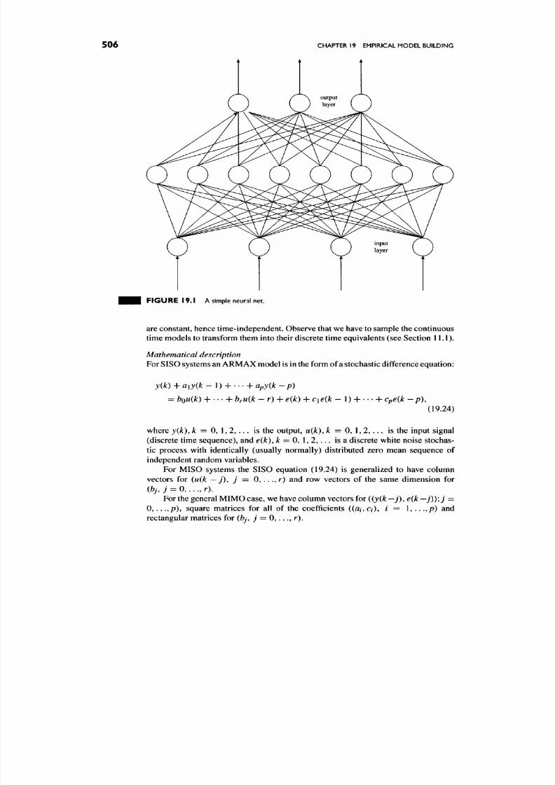
8/17/2019 Process Modelling and Model Analysis-Hangos-Cameron
http://slidepdf.com/reader/full/process-modelling-and-model-analysis-hangos-cameron 523/560
506
CHAPTER 19 EMPIRICAL MODEL BUILDING
FIGURE 19 .1 A simple neural net.
are constant, hence time-independen t. O bserve that we have to sample the continuous
time mo dels to transform them into their discrete time equivalents (see Section 11.1).
Mathematical description
For SISO systems an ARM AX m odel is in the form of a stochastic difference equation:
y{k)
+
a\y{k
- 1) H h
apy{k - p)
= bouik)
H
h
bru(k - r)-\- eik)
-f-
cie(k
- 1)
H
h
Cpe(k
- / ? ) ,
(19.24)
where y{k), /: = 0, 1, 2 , . . . is the output, u{k), A; = 0, 1, 2 , . . . is the input signal
(discrete time sequence), and
e{k),
^ = 0, 1, 2 , . . . is a discrete white noise stochas
tic process with identically (usually normally) distributed zero mean sequence of
independent random variables.
For MISO systems the SISO equation (19.24) is generalized to have column
vectors for
(u(k
—
j), j =
0,..., r) and row vectors of the same dimension for
{bj. 7 = 0 , . . . , r ) .
For the general M IM O case, we have column vectors for
((y(k — j), e{k — j))\j =
0,...,/?), square matrices for all of the coefficients ((a/,
Q ) ,
/ =
1,...,/?)
and
rectangular matrices for
(bj,
7 = 0 , . . . , r ) .
8/17/2019 Process Modelling and Model Analysis-Hangos-Cameron
http://slidepdf.com/reader/full/process-modelling-and-model-analysis-hangos-cameron 524/560
8/17/2019 Process Modelling and Model Analysis-Hangos-Cameron
http://slidepdf.com/reader/full/process-modelling-and-model-analysis-hangos-cameron 525/560
5 0 8 CHAPTER 19 EMPIRICAL MODEL BUILDING
In order to keep notation low the mathematical description is only given for the
SISO case. For a more detailed treatment of the subject we refer to the recent book
by Haber and Keviczky [181].
Mathematical description
The parametrized version of the most popular and widely used nonlinear dynamic
black-box model structures can be regarded as second order polynomial type
extensions of the linear time-invariant ARMAX model in Eq. (19.24).
The more general of these approximations is the so-called
parame tric Volterra
model which is in the following general form:
(19.26)
where the discrete linear filters
tfv.( (-1)) ^ g "( g |~ ' | ) ^^H,L,V
are understood as
Ha nb
J^aJy{k-j) = J2^Ju{k-j),
j=0 7=0
We see that the variable q^~^^ in the polynomials
A^
and
B^
above is the so called
backward shift operator which acts on a signal z as q^~^\{k) = z{k — 1). From the
above filter equations it follows that we have infinite sums in the model structure
(19.26) in the form of
00
H''(q^-^^)u{k) = J^hJu{k -j) .
It is then up to the user to find appropriate large integers N\', N^ and
A^^,
j = 0,., .,Ny to
truncate the above infinite su ms.
There are three types of terms in the right-hand side of
the
parametrized Volterra
model (19.26):
• the first term is purely linear with the upper index ^,
• the second is a quadratic with upper index ^, and
• the third is the general bilinear (2nd order) term with upper index ^.
If only the first two terms are in the Volterra m odel, that is A^ = 0 or
—z = 0 / = 0 A^^
Ai;.(,(-')) "' ' "^'
then it is called a generalized Hammerstein model.
8/17/2019 Process Modelling and Model Analysis-Hangos-Cameron
http://slidepdf.com/reader/full/process-modelling-and-model-analysis-hangos-cameron 526/560
BLACK-BOX MODELLING
509
Structural parameters
The structural parameters fall into two categories:
• the order of the approximation that is the integers
N]-,
N^, N^, (N^J,
7 = 0 , . . . ,
N^)
• the set of variables present in the vectors
y(k)
and
u{k)
and their dimension,
that is
\y\ = n, \u\ = m.
Parameter estimation
Because the no nlinear second order expansion is linear in its param eters we can apply
the parameter estimation method of the linear ARMAX model structures as before.
The structural parameters can be estimated the same way as in the general MO D E L
STRUCTURE ESTIMATION
problem statement.
The following simple example shows how we can construct the mathematical
form and the parameters of various nonlinear models.
• • • EXAMPLE 19.3.5 (Simple dynamic nonlinear model examples). Let us start
with a simple SISO Hammerstein model in the form of
y{k) = h\u{k) + h\u(k - 1) + h^u^{k) + h^u^{k - 1), (19.27)
where A | = 1, N^ = l,N^ = 0. Here the parame ters are the scalars
where h ^ and h\ are the parameters of the linear subm odel.
If we extend the above model to obtain a parametrized Volterra model with
N^ =z 1, we get
y(k) = h^u(k)
+
h\u(k
- 1) +
h^u^ik)
+
h^u'^(k -
1)
+ h\Qu{k)u{k - 1) + h\^u{k - \)u{k - 2). (19.28)
Here we have two new structural parameters
A2o —
^' ^21
— ^ •
^ ^^ complete set of
parameters is then
[ " Q » " J »
l^Q
1 f^l 1 1 0 ' 1 1 J
• • • where
/ IQ ,
h\, h^ and h^ are the parameters of the Hammerstein sub-m odel.
19.3.4. Identification for Black-box Modelling
Identification as a tool for model calibration, that is model parameter and structure
estimation for dynamic m odels is described in Section 12.4. The main emph asis there
has been placed on parameter estimation.

8/17/2019 Process Modelling and Model Analysis-Hangos-Cameron
http://slidepdf.com/reader/full/process-modelling-and-model-analysis-hangos-cameron 527/560
5 10 CHAPTER 19 EMPIRICAL MODEL BUILDING
Black-box modelling mainly needs structure estimation over special general and
flexible model structures, called black-box m odel structures, which have simple struc
ture indices. The subsection Parameter estimation given for the black-box model
structures above gives guidelines on how to perform the model structure estimation
relevant to the structure in que stion.
It is important to note that the result of identification is always in terms of
• estimate of the structural param eters,
• estimate of parameters of the model with the "best structure",
• uncertainty associated with the estimate(s).
19.3.5. The Information Transfer between the Black-box
Model Element and the Overall Model
Having validated a black-box model based on measured data, the next step is to
put together the overall grey-box model. This section is about how to incorporate
black-box elements into a white-box structure.
Black-box Functional Relationship
The result of model validation is not only the structure and best parameters of the val
idated black-box submodel but also uncertainty ranges, usually confidence intervals
associated with each of the parameters in the model. Then it is important to transfer
the information contained in the static model with parametric uncertainty into the
white-box structure.
If
a
black-box n onlinear function-type relationship
y =
/(jc,
p)
has been validated
to obtain an estimate of the scalar param eters in the form of/? —
Ap < p < p
— Ap,
then the nonlinear function may damp or amplify the effect of the uncertainty in the
parameters 2 Ap. We can use the same principle as in the case of parametric sensitivity
for static mod els, and derive the following estimate of the uncertainty in the variable y
9 /
Ay = max —(jc)
x€Domx dp
Ap. (19.29)
The above estimate can be easily g eneralized to the case of vector variables p:
Ay=
max J/ , ; ,W | oA p, (19.30)
where Jfx is the Jacobian matrix of the fu nc tio n/ with respect to the variables JC .
Black-box Submodel
If a black-box submodel is to be imbedded into a white overall model structure, then
we essentially have the same case as the relationship with mod els on different hier
archy levels in hierarchical modelling (see in Chapter 9). In the case of an unknown
or partially known mechanism, we may use the methodology of multi-scale mod
elling, given by a model hierarchy driven by characteristic sizes (see in Section 9.2
in Chapter 9) to get an empirical model of the missing part of a grey-box model.
Having performed the lower level modelling and the validation of this model, the
8/17/2019 Process Modelling and Model Analysis-Hangos-Cameron
http://slidepdf.com/reader/full/process-modelling-and-model-analysis-hangos-cameron 528/560
TRAPS AND PITFALLS IN EMPIRICAL MODEL BUILDING
5 I I
information transfer requires the computation of volumetric integrals (averaging) for
both the independent and dependent model variables.
19.4. TRAPS AND PITFALLS IN EMPIRICAL MODEL BUILDING
The various tools and techniques available for empirical model building indicate that
it is usually not easy to obtain a reliable and easy-to-use black-box model which fits
our purpose. We may fall into traps or come up with poor quality m odels. This section
is about how to detect that we are approach ing or have already fallen into som e traps
and then how to recover from them. In most cases these problems can be avoided if
proper prevention steps are carried out.
The traps and pitfalls are described in the following items:
•
Causes and consequences
—This item gives a detailed explanation of the
problem one m ay have with its possible causes and con sequences.
• Detection—The possible ways of detecting the problem are briefly described
here.
• Prevention—The possible precautions and steps to avoid the problem are also
given.
19.4.1.
Interpolation and Extrapolation: the Validity Range
Causes and consequences
The majority of empirical models are only valid within the closed (and usually con
vex) domain spanned by the measurement points. Therefore one should ensure that
the measurement (or collocation) points cover the entire region: otherwise an ill-
conditioned or poorly trained mod el is obtained. For further details on ill-conditioned
models see section 19.4.3.
Detection and prevention
For nonlinear models the validity range is very narrow: one should not use them
outside the region spanned by the measurement (or collocation) points.
Static Models
The main difference between linear and nonlinear static models from the viewpoint
of their validity range is that nonlinear models are often very poor outside of their
validity rang e. Therefore, their specification should contain an ex plicit description of
the required validity range and the measu rement p oints available for model validation
should span the entire validity range.
The following example illustrates the fit of a polynomial to a reaction kinetic
expression.
• • • EXAMPLE 19.4.1 (The fit of a polynomial to a nonlinear reaction kinetic
express ion). Con sider the following reaction kinetic expression
^1.5
1 -
LA
over the validity range 0.2 <CA< 0.8.
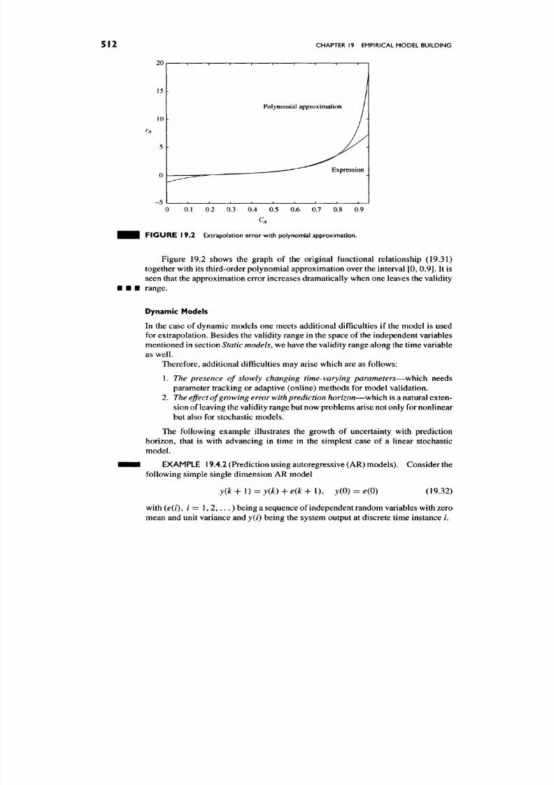
8/17/2019 Process Modelling and Model Analysis-Hangos-Cameron
http://slidepdf.com/reader/full/process-modelling-and-model-analysis-hangos-cameron 529/560
512
CHAPTER 19 EMPIRICAL MODEL BUILDING
20
15
10
-5
Polynomial approximation
_J I I I I L_
Expression
_i i_
0 0.1 0.2 0.3 0.4 0.5 0.6 0.7 0.8 0.9
CA
F I G U R E 1 9 . 2 Extrapolation erro r with polynomial approximation.
Figure 19.2 shows the graph of the original functional relationship (19.31)
together with its third-order polynom ial approximation over the interval [0 ,0 .9] . It is
seen that the approximation error increases dramatically w hen one leaves the validity
range.
Dynamic Models
In the case of dynam ic m odels one m eets additional difficulties if the m odel is used
for extrapolation. Besides the validity range in the space of the independ ent variables
mentioned in section
Static models,
w e have the validity range along the time variable
as well.
Therefore, additional difficulties may arise which are as follows:
1.
The presence of slowly changing time-varying parameters—which needs
parameter tracking or adaptive (online) methods for model validation.
2. The effect of growing error with prediction horizon
— which is a natural exten
sion of leaving the validity range but now problems arise not only for no nlinear
but also for stochastic models.
The following example illustrates the growth of uncertainty with prediction
horizon, that is with advancing in time in the simplest case of a linear stochastic
model.
EXAMPLE 19.4.2 (Prediction using autoregressive (AR) mo dels). Consider the
following simple single dimension AR model
y(k + 1) = y{k) + e(k + 1) , y(0) = e(0) (19.32)
with {e(i), i = 1,2,...) being a sequence of independent random variables with zero
mean and unit variance and y{i) being the system output at discrete time instance /.
8/17/2019 Process Modelling and Model Analysis-Hangos-Cameron
http://slidepdf.com/reader/full/process-modelling-and-model-analysis-hangos-cameron 530/560
TRAPS AND PITFALLS IN EMPIRICAL MODEL BUILDING 5 I 3
If we perform prediction with the model above for A: = 1,2,..., the following
explicit formulae is obtained for the predicted output:
k
y{k) = Yle{k),
A: =
0 , 1 , . . . .
(19.33)
i=0
As ie{i),
i
= 1, 2 , . . . ) is a sequence of independent random variables with zero
mean and unit variance, the variance ofy{k) is simply the sum of the variances of the
variables on the right-hand side of Eq. (19.33):
• • I which clearly grows in time in a mono tonic way.
19.4.2.
Non-informative Models
Causes and consequences
A model is not informative with respect to one or more of its variables and/or para
meters if its dependent variable(s) do not change by changing them. It means that
non-informative models are not sensitive enough with respect to their independent
variable(s) and/or parameters.
Detection and prevention
The detection is performed by calculating the sensitivities of the validated model by
all of its parameters and independent variables. The calculation can be performed
analytically as it has been desc ribed in Section 19.3.2 and then check if
the
particular
sensitivities differ significantly from zero.
Note that it is not always unfortunate if one figures out that there is a non-
informative part in the model. The non-informative "unnecessary" part of the model
should be simply left out from the model by neglecting the corresponding terms or
considering the corresponding factor to be constant. This manipulation is then seen
as a kind of mode l simplification.
The following simple example shows how one can visualize the notion of a
non-informative functional dependence.
• ^ H EXAMPLE 19.4.3 (Non-informative functional dependence). Figure 19.3
shows the graph of a two-variable nonlinear functional relationship. It is seen that
there is a wide "flat" area of the function. Th is indicates the region w here it does not
• • • depend on its variables, that is wh ere it is non-informative.
19.4.3.
Ill-conditioned or not Properly Trained Models
Causes and consequences
If the parameter and/or independent variable space is not covered by sufficient data
then we end up with ill-conditioned or poorly trained models. Such models lead to
uncertain, non-decisive or in some cases even non-correct decisions if one uses the
model for control and/or diagnostic purposes or tries to use the model output for any
kind of further processing.

8/17/2019 Process Modelling and Model Analysis-Hangos-Cameron
http://slidepdf.com/reader/full/process-modelling-and-model-analysis-hangos-cameron 531/560
514
CHAPTER 19 EMPIRICAL MODEL BUILDING
FIGURE 19 .3 A non-informative functional relationship.
Detection and prevention
The method of detection depends on the type of black-box model which is used:
1. Static and dynamic models linear in parameters
In this case, we can easily and safely detect ill-conditioned models via the
covariance matrix of the parameters through the correlation coefficient
p
of
the estimated parameters which is computed according to the formulae:
A ;
[COy[p]]ij
SpjSpj
(19.35)
where [COV{p}]/y is the off-diagonal element of the covariance matrix and
Spi^Spj are the corresponding diagonal elements. Note that 1 > p > — 1
is a measure of the dependence between the estimated values: if it is small
compared to 1 then we have a good, uncorrelated estimate for the param eters,
otherwise the model is ill-conditioned or not properly trained.
We have already seen an example of this phenomena in Section 12.5.3
where the estimated coefficients were highly correlated. Note that this poor
quality estimate could have been avoided by experiment design, by properly
selecting the me asurement point in advance (see Sections 12.3 and 12.4).
2.
Neural net models
There are theoretical investigations on how many training sam ples are needed
to properly train a neural net of a given arch itecture, say a feedforward three-
layer neural net of a given number of neurons in the input, hidden and output
layers [182]. This number can be rather high in practical cases compared with
the number of available sam ples. Therefore, it is often the case that one uses
a poorly trained neural net in real applications. Example 19.4.4 contains a
concrete example on the number of necessary training samples.
Poorly trained neural nets for classification may even misclassify
unknown samples.

8/17/2019 Process Modelling and Model Analysis-Hangos-Cameron
http://slidepdf.com/reader/full/process-modelling-and-model-analysis-hangos-cameron 532/560
FURTHER READING 5 I 5
The usual way of testing whether the neural net is properly trained is to divide
the training samples into two subsets. The first one is used for training and then the
second is to test the computation error of the net.
• • • EXAMPLE 19.4.4 (Poorly trained neural network mo dels for fault classification
[183]). Let us consider a three-layer feedforward neural net for fault classification
with six neurons in the output (that is six fault types are conside red) and three neurons
in the hidden layer with all together 45 weights. If we want the net to perform the
classification with less that 10% error, then we need to have 300 samples and train
the network with them with a precision of 5% . This sample size grows to 2300 if we
• • • need less than 1% classification error.
More about neural networks in chemical engineering can be found in [184].
19.5.
SUMMARY
Process models usually contain black-box model elements imbedded in a white-box
model structure, therefore the methods and tools of empirical model building are
of primary practical importance. The revised and extended SEVEN STEP MODELLING
PROCEDURE provides a common framework for such grey-box models, incorporating
the steps needed for empirical model building.
This chapter discusses the most commonly used black-box model structures in
process modelling: linear and nonlinear static model structures including neural net
works, as well as linear dynamic ARMAX and nonlinear dynamic Volterra and
Hammerstein models. Together with the mathematical description, the structural
parameters and the proposed identification method for each of the black-box model
types are given.
Special emphasis is put into unusual and sensitive points related to empirical
mod el building such as the sensitivity of the model output with respect to its parameters
and variables, the information transfer between the black-box subm odel and its white-
box environment and to the traps and pitfalls in empirical model building.
19.6.
FURTHER READING
There is a vast amount of literature on emp irical model bu ilding typically in fields of
high complexity and practical importance such as
• Modelling of complex reaction kinetic expressions
An empirical kinetic model has been developed for the extraction of black
cumin seed oil with supercritical carbon dioxide as solvent using neural net
model in [185].
A laminar falling film slurry photocatalytic reactor used for wastewater
treatment is modelled in [186] using a simplified experimental model with
only five dimensionless parameters. The parameters can be readily estimated
from process data. A study of the sensitivity of the model to variations of the
models parameter and validation of the model with experimental data are also
presented.
8/17/2019 Process Modelling and Model Analysis-Hangos-Cameron
http://slidepdf.com/reader/full/process-modelling-and-model-analysis-hangos-cameron 533/560
516
CHAPTER
19
EMPIRICAL MODEL BUILDING
• Modelling of unusual complex processes
A
grey-box model is constructed to describe the turbulent burning between
vertical parallel walls with a fire-induced flow in [ 187]. Transport equations for
mass,
momentum, chemical components and enthalpy are combined with an
empirical model for estimating the flame radiation energy to the burning w all.
A general systematic procedure is presented to support the development and
statistical verification of empirical dynamic process model in [188]. Methods are
presented to address structural identifiability and distinguishability testing, as well as
optimal design of dynam ic experiments for both model discrimination and improving
parameter precision.
19.7. REVIEW QUESTIONS
Q19.1.
In the context of the systematic SEVEN STEP MODELLING PROCEDURE oudined
in Section 2.3 of Chapter 2 describe how black-box model elements of various types
naturally arise. (Section 19.2)
Q19.2. What are the three main types of black-box mo del elements? D escribe their
general mathem atical form together with their white-box environm ent, (section 19.2)
Q19.3.
Explain the importance of parametric sensitivity in empirical modelling.
What is the relationship between variable sensitivity and model linearization?
(Section 19.3)
Q19.4.
Describe the linear and nonlinear static model structures suitable for
empirical model building. Give their mathematical description and their structural
parameters. (Section 19.3)
Q19.5. Describe the linear and nonlinear dynamic model structures suitable for
empirical model building. Give their mathematical description and their structural
parameters. (Section 19.3)
Q19.6. How would you characterize the information transfer between the black-box
submodel and the white overall model structure? Wh at is the role of the sen sitivities
in this transfer? (Section 19.3)
Q19.7. What are the most common traps and pitfalls in empirical model building?
Desc ribe the problem, the detection and the prevention me thod(s). (Section 19.4)
19.8.
APPLICATION EXERCISES
A19.1. Develop a grey-box model of a plug-flow tubular isotherm catalytic reactor
where the heterogeneous reaction kinetic expression is unknown . Assum e a function-
type black-box model. (Sections 19.2 and 19.3)
A 19.2. Develop a grey-box model of a plug-flow tubular isotherm catalytic reactor
where the heterogeneous reaction kinetic expression is unknown. Use a model-type
black-box model. Compare it with a hierarchical model driven by the characteristic
sizes of the same system described in Section 9.2. Compare it also with the model
developed in the previous exercise. (Sections 19.2 and 19.3)

8/17/2019 Process Modelling and Model Analysis-Hangos-Cameron
http://slidepdf.com/reader/full/process-modelling-and-model-analysis-hangos-cameron 534/560
APPENDIX: BASIC
MATHEMATICAL TOOLS
A . I .
RANDOM VARIABLES AND THEIR PROPERTIES
A.
I. I. Random Variables with Gaussian (Normal) Distribution
Scalar Case
Let us take the one dimensional ID scalar case
first,
hat is a real-valued random
variable
?: ^(ft>), coeQ., ^i(o)e1Z. (A.l)
The random variable is normally distributed or has a Gaussian (Normal) Distribution
^--Afim^cr^), (A.2)
if
its
probability density function/^ is in the following form:
fy(x) = ^^c-^'-^ '^ /^-\ (A3)
where m is the
mean value
and a^ is the
variance
of the random variable. Both m
and a^ are real numbers. The shape of the ID Gaussian probability density function
is shown in
Fig.
A .l .
The mean value of the random variable ^ with probability density function/^ is
computed as
= / ^ , ( .
[^}= xftix)<ix. (A.4)
517

8/17/2019 Process Modelling and Model Analysis-Hangos-Cameron
http://slidepdf.com/reader/full/process-modelling-and-model-analysis-hangos-cameron 535/560
518
APPENDIX: BASIC MATHEMATICAL TOOLS
F I G U R E A . I One-dimensional Gaussian probability density function.
The covariance between two scalar random variables ^ and 0 is defined as
COV{?,
0} =
E{(^ - E{^})(^ - E{^})}. (A.5)
The variance of a random variable ^ is just a covariance of that variable with
itself,
i.e.
(A.6)
^[^} =
C OV { ^ §} = E{(§ - E{?})2}.
Vector-valued Random Variables
Let us now assume that ^ is a vector-valued random variable, i.e.
(A.7)
Then its mean is also a real-valued vector
m e W^
and its variance is a matrix called
its
covariance matrix.
C O V { |} = E { ( ? - E { ? } ) ( ? - E { f } ) ' r } .
(A.8)
It is important to note that covariance matrices are positive definite symmetric
matrices, i.e.
The probability density functio n/^ of a vector-valued random variable is a scalar-
valued multivariate function, i.e.
fr-T^
n.
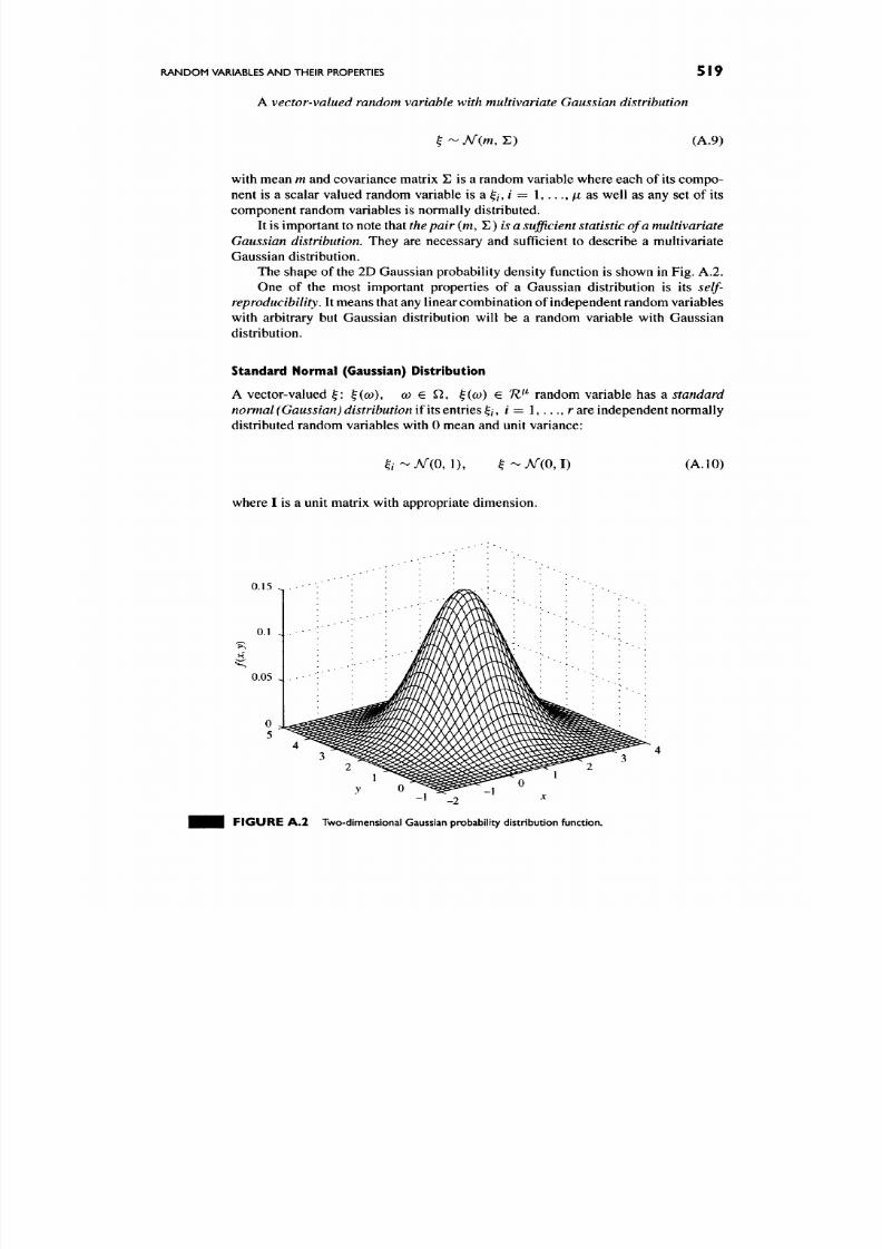
8/17/2019 Process Modelling and Model Analysis-Hangos-Cameron
http://slidepdf.com/reader/full/process-modelling-and-model-analysis-hangos-cameron 536/560
RANDOM VARIABLES AND THEIR PROPERTIES 5 19
A vector-valued random variable with multivariate Gaussian distribution
^ -ATCm, E)
(A.9)
with mean
m
and covariance matrix E is a random variable where each of its compo
nent is a scalar valued random variable is a ^/, / = 1 , . . . , jit as well as any set of its
component random variables is normally distributed.
It is impo rtant to note that the pair (m,T>)isa sufficient statistic of a multivariate
Gaussian distribution. They are necessary and sufficient to describe a multivariate
Gaussian distribution.
The shape of the 2D Gaussian probability density function is shown in Fig. A.2 .
One of the most important properties of a Gaussian distribution is its self-
reproducibility. It mean s that any linear combination of independ ent random variables
with arbitrary but Gaussian distribution will be a random variable with Gaussian
distribution.
Standard Normal (Gaussian) Distribution
A vector-valued ^: ^(co),
co e Q, ^(w) e TZ^
random variable has a
standard
normal (G aussian) distribution if its
cnir'iQs^i,
/ = , . . . , r are independent normally
distributed random variables with 0 mean and unit variance:
^i-^Af
(0,1).
?~Ar(0,I)
(A. 10)
where I is a unit matrix with appropriate dimension.
0.15
0.1 J
0.05
F IG U R E A . 2 Two-dimensional Gaussian probability distribution function.

8/17/2019 Process Modelling and Model Analysis-Hangos-Cameron
http://slidepdf.com/reader/full/process-modelling-and-model-analysis-hangos-cameron 537/560
8/17/2019 Process Modelling and Model Analysis-Hangos-Cameron
http://slidepdf.com/reader/full/process-modelling-and-model-analysis-hangos-cameron 538/560
HYPOTHESIS TESTING 52 I
with E^/^ being a positive definite symmetric matrix, too. Then the vector-valued
random variable
^^ = E - ^ / 2 § - m (A .1 4)
is a standard Gaussian vector-valued random variable.
A.2.
HYPOTHESIS TESTING
Hypothesis testing is a standard procedure in mathematical statistics to get an evalu
ation of whether or not a particular relation holds for a random variable. The way to
perform a hypothesis test is described below as a standard algorithmic problem.
HYPOTHESIS I^STIN G
Given:
•
a sample
S(?) = { ? l ,$ 2, . . . ,?n } (A.15)
consisting of independent measurements as elements ^/, / = 1 , . . . , n taken
from a joint underlying random variable §;
• a
hypothesis
in the form of a relation on the statistics of the random variable
in the sample, e.g.
HQ
: m = mo
(A.16)
with mo is a given constant, the hypothetical value for the mean value m;
• an assumption on the underlying distribution of the sample elements, e.g.
Gaussian with known variance A;
• a significance level 0 < £ < 1 which is the level of confidence to which you
test your hypothesis.
Question:
Is the hypothesis // Q true on the significance level E based on measurements in the
sample S (?)?
Method:
The hypothesis testing is usually done in three subsequent steps:
1. Com pute an estimate of the statistics present in the hypothesis relation, e.g.
m = E{ ?} 2. M {S(^)} = ^ i ^ , (A. 17)
n
where M stands for the sample arithmetic mean.
2. Construct a statistic of a normalized random variable with a known distribu
tion, e.g.
M { S ( ^ ) } - m o
^ _ ^ j^(Q^ J) (A.18)
V A
3. Compa re the computed normalized statistics to its "critical" value (e.g.
Merit)
corresponding to the given significance level s. The critical values are given
usually in the form of tables.
Ifu <
Merit ^^^^
accept the hypothesis otherwise
reject it.
8/17/2019 Process Modelling and Model Analysis-Hangos-Cameron
http://slidepdf.com/reader/full/process-modelling-and-model-analysis-hangos-cameron 539/560
522
APPENDIX: BASIC MATHEMATICAL TOOLS
A.3.
VECTOR AND SIGNAL NORMS
If we have objects of a non-scalar nature, for example vectors, matrices, functions or
signals, we measure their magnitude by using norms. Norms are the extensions of a
length of a vector applied to other objects of non-scalar nature forming a so-called
vector space.
The set of elements
X
is called a v ector space if
• if jci, JC2 € X then jc* = {x\ -\-X2) G X,
• if jci €
X
then
x* = ax\ e X
for any
a elZ,
• there is a zero element
XQ eX
for which
x\-\-xo = x\
holds for every jci
e X.
A scalar-valued function p ( ) : Z -> 7?. is a norm on a vector space X if
•
p{x)
> 0, VJC € X,
• yo(jc) = 0 O JC = 0 € X, (x = 0 is the zero element),
•
p{x + y) < p{x)
-[•
piy)
(triangular inequality).
A . 3 . I .
Vector Norms
The w-dimensional vectors with real-valued entries
x =
U i, JC2,..., Jc„]^ form a
vector space c alled TZ^. There are different known and useful norms defined over the
vector space
7?."
which are as follows:
1.
Euclidean norm or 2-norm
ll lb
= V S ^
(A.19)
2.
Maximum norm or oo-norm
\\x\\oo = max(\xi\) (A.20)
/
A.3.2. Signal Norms
Discrete time linear systems are usually described by linear difference equations
which contain
discrete time signals
f{k), ^ = 0, 1, Discrete time signals can be
sampled data
of continuous time signals. Discrete time signals form a vector space.
A discrete time signal may be scalar-valued or vector-valued, i.e.
fik) e 7^, F(k) e 7^'^
We shall use two types of
norm s of a discrete time signal:
the
infinity norm
and
the 2-norm
ll/lloo = sup\f(k)l IIFIloo = sup||F(fc)||oo, (A.21)
k k
00 00
ll/lll
= E
/ ^ ( * ) '
"^"2 = E Il^( >ll2- (A.22)
^=—00
k=—oo
8/17/2019 Process Modelling and Model Analysis-Hangos-Cameron
http://slidepdf.com/reader/full/process-modelling-and-model-analysis-hangos-cameron 540/560
MATRIX AND OPERATOR NORMS 523
The induced norm of an operator Q on the vector space X induced by a norm
II • II on the sam e space is defined as
iinii IIQWII . . oa^
IIQII = sup •• •• . (A .23)
\\x\\ = \ \W\
^A. MATRIX AND OPERATOR NORMS
Ma trices can be seen as linear operators transforming vectors from a vector space like
TZ' to another vector space which can be the same or a different one like 7^'". For
rectangular matrices when m ^ n and T e W^^^ we have different vector spaces
and for square matrices when
n = m
they are the same vector space.
The "magnitude" of a matrix is also characterized by its norm. Similarly to the
case of vectors and matrices there are various norms app licable for matrices. The most
important ones are the so-called induced norms where the matrix norm
is
derived using
an already defined vector norm. The induced N-norm of a square matrix T € TZ^^^^
is defined as
l |T|k = sup - 7 - 7 — , (A.24)
xeU" \W\N
where || • ||;v is a vector norm.
The norm of an operator T acting on a signal space is defined similarly but now
we have a signal norm instead of a vector norm in || • HAT.
A.4.1. Quadratic Forms and Definite Matrices
Quad ratic forms are important expressions in loss functions of both parameter estima
tion and control problem formulations. A quadratic form is an expression containing
a vector jc € TZ^ and a square matrix Q e1Z^^^:
qg = x^Qx,
(A.25)
Observe that the value of the quadratic form itself is a real num ber, that is
x^Qx
e n,
A quadratic form is definite if it has the same sign for every possible vector x.
The matrix Q present in the quadratic form is called definite if the corresponding
quadratic form is definite. In particular, a quadratic matrix Q is called
•
positive definite, ifx^Qx
> 0,
• negative
definite,
ifx^Qx < 0 ,
•
positive semidefinite, ifx^Qx >
0 ,
• negative semidefinite, ifx^Qx < 0 ,
•
if neither of the above conditions hold it is indefinite
for every possible
X
e IZ^.

8/17/2019 Process Modelling and Model Analysis-Hangos-Cameron
http://slidepdf.com/reader/full/process-modelling-and-model-analysis-hangos-cameron 541/560
524
APPENDIX: BASIC MATHEMATICAL TOOLS
A.5.
GRAPHS
Graphs in general are combinatorial objects used for describing the structure of sets
and set systems. A graph G in the mathematical sense is specified by a pair of related
sets
G = ( V , £ ) ,
where V = [v\, V2,...,
Vn)
is the set of vertices and E is the set of edges which
contains vertex-pairs, i.e.
E =
{(v/,
vj)
I v/,
vj e V}.
A directed graph
G is a graph whose edge set
E
contains
ordered vertex-pairs.
It
means that (v/,
vj) e E
follows from (vy, v/) G £ in the undirected ca se but for
directed graphs (v/, v/)
e E
does not imply (v/, Vj)
e E.
Graphs and directed graphs can be conveniently visualized by figures where we
depict vertices as points or small circles and edges (v/, Vj) as intervals joining the
points labelled v/ and
Vj
or directed arrows pointing to
Vj
and starting at v, in case of
directed graphs.
A sequence P = ( v i , . . . , v„), v/ € V of vertices in a graph G = (V, E), forms a
path in G, if (v/, v/_|_i) G
E,
i.e. the subsequent elements in the sequence are joined
by an edge. A d irected path is a vertex sequence in a directed graph G = (V, E)
where the subsequent elements are joined by a directed edge pointing to the direction
of increasing sequence numbers, i.e. (v/, v/4.1) €
E.
The
length of a (directed) path
is the number of edges one traverses while traversing the path.
A (directed) circle is a (directed) path where the starting and ending vertices
coincide, i.e. vi = V/ . A
(directed) loop
is an edge whose starting and en ding vertex
is the sam e, i.e. (v/, v/). A (directed) loop is a circle of length 1.
A subgraph G' = ( V , £') of a (directed) graph G = (V ,£ )w ith V' c V, £:' c £:
is
connected (strongly connected)
if there is at least one (directed path) connecting
any vertex pair (v i, V2), vj, V2 6 V . A strongly connec ted subgraph is called a strong
component of the original graph.
Weighted graphs
are graphs where we put a weight, usually a real or integer
number to each of the edges. The weight function w is then defined as
H'(v/, Vj) = W ij, V(v/, Vj) e E .
The weighted graph Gw is denoted by Gw = (V, E; w). Weighted directed graphs
Gw =
(V ,
E; w)
are defined analogously.
Th e va lue of a (directed) path in a weighted (directed) graph is the product of
the weights on the edges one traverses w hile traversing the path, i.e.
H^((Vl, . . ., Vn))
=
P I W(V,-, V/+i).
The basic notions of graphs are illustrated on a simple example shown in
Fig.
A.3.
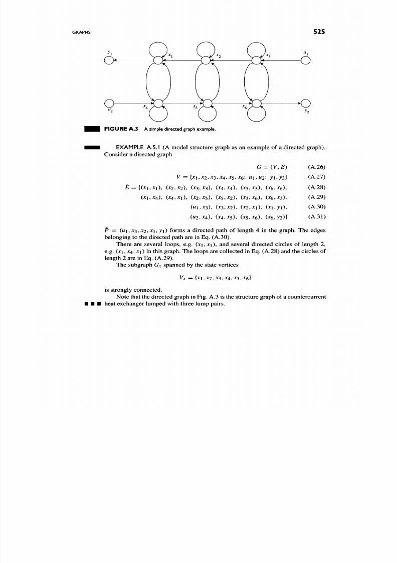
8/17/2019 Process Modelling and Model Analysis-Hangos-Cameron
http://slidepdf.com/reader/full/process-modelling-and-model-analysis-hangos-cameron 542/560
GRAPHS
525
O
a
o
o
F I G U R E
A. 3 A simple directed
graph)
example.
EXAMPLE A.5.1 (A model structure graph as an example of a directed graph).
Consider a directed graph
G = (V, E) (A.26)
V = {xux2,x3,x4,xs,xe; MI,M2; yi^yi]
(A.27)
E = {(x\,Xi), (X2,.^2), (X3.X3), {X4,X4), (X5,X5), {Xe,Xe), (A.28)
(xuXi),
(X4,-^l), {X2.X5), {xs,X2), (-^3,-^6), (^6.-^3), (A.29)
( MI , X 3 ) ,
(^3,^2), (-^2,^1), (x\.yi), (A.30)
(U2,X4),
(X4,X5),
(X5,X6),
(Xe.yi)}
(A.31)
P =
(MI,.^3,^:2,^1,^1)
forms a directed path of length 4 in the graph. The edges
belonging to the directed path are in Eq. (A.30).
There are several loops, e.g.
(x\,X]),
and several directed circles of length 2,
e.g. (xi, X4, xi) in this graph. The loops are collected in Eq. (A.28) and the circles of
length 2 are in Eq. (A.29).
The subgraph Gx spanned by the state vertices
Vx = {X{,X2,X3,X4,Xs,Xe}
is strongly connected.
Note that the directed graph in Fig. A.3 is the structure graph of a countercurrent
heat exchanger lumped with three lump pairs.

8/17/2019 Process Modelling and Model Analysis-Hangos-Cameron
http://slidepdf.com/reader/full/process-modelling-and-model-analysis-hangos-cameron 543/560
This Page Intentionally Left Blank

8/17/2019 Process Modelling and Model Analysis-Hangos-Cameron
http://slidepdf.com/reader/full/process-modelling-and-model-analysis-hangos-cameron 544/560
BIBLIOGRAPHY
[1] D.M. Himmelblau and K.B. Bishoff, P rocess Analysis and
Simulation,
Wiley, New York, 1968.
[2] M.E. Davis, Num erical Methods and Mod elling for Chem ical E ngineers, Wiley, New York,
Chichester, Brisbane, 1984.
[3] J.B. Riggs, An In troduction to Numerical Methods for Chem ical E ngineers (2nd edn), Texas
University Press, Texas, 1994.
[4] R.D. Rice and D.D . Do , Applied
Mathematics
and Modelling for Chem ical
E ngineers,
W iley, New
York, 1995 .
[5] R. Aris, Mathematical Modelling Techn iques, Pitman, London, 1978.
[6] M.M. Denn, Process Modelling, Longman, New York and London, 1986.
[7] M. Minsky, "Mo dels, minds, machines". Proceedings IFIP Congress, pp. 45 -49 , 1965.
[8] Sdu Uitgevers, Methods for the Calculation of Physical E ffects, CPR 14E (Pt2) , Committee for
Prevention of Disasters, The Netherlands, 1997.
[9] G.E. Davis,
A Handbook of Chemical Engineering 2nd edn,
Davis Bros., Manchester, England,
1904.
[10] W.H. Walker, W.K. Lewis, and W H. Mc Adams, Principles of Chemical Engineering, McGraw-Hill
Book C o. Inc., New York, London, 1923.
[11] J.C. Olsen, Unit Processes and Principles of Chemical Engineering, Macmillan and Co., London,
1932.
[12 ] T.J. William s, Systems E ngineering for
the
Process In dustries, McGraw-Hill, New York, 1961.
[13] R.B. Bird, W.E. Stewart, and E.N. Lightfoot, Transport Phenomena, Wiley, New York, 1960.
[14] L. Ljung, System Identification: Theory for the User, Prentice Hall Inc., New Jersey, USA , 1987.
[15] R. Penrose, The Emperor s N ew
Mind,
Vintage, 1990.
[16] J.M. Honig, Thermo dynamics: Principles Characterizing Physical and Chemical Processes,
Elsevier, Amsterdam, Oxford, New York, 1982.
[17 ] G. Astarita,
Thermodynamics: An Advanced Textbook for Chemical E ngineers,
Plenum Press, New
York-London, 1989.
527
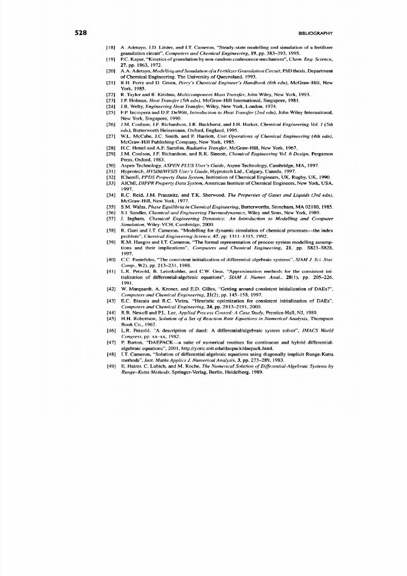
8/17/2019 Process Modelling and Model Analysis-Hangos-Cameron
http://slidepdf.com/reader/full/process-modelling-and-model-analysis-hangos-cameron 545/560
528 BIBLIOGRAPHY
[18 ] A. Adetayo, J.D. Litster, and IT, Cam eron, "Steady-state mod elling and simulation of a fertilizer
granulation circuit",
Computers a nd Chemical Engineering,
19, pp. 383 -393 , 1995.
[ 19] P.C. Kapur, "Kinetics of granulation by non-random coa lescence mechanism", Chem. Eng. Science,
27, pp.
1863, 1972.
[20] A. A. Adetayo, Modelling and Simulation ofa Fe rtilizer Granulation
Circuit,
PhD
thesis, Department
of Chemical Engineering, The University of Queensland, 1993.
[21] R.H. Perry and D. Green, Perry's Chemical Engineer's Handbook (6th edn), McGraw-Hill, New
York, 1985.
[22 ] R. Taylor and R. Krishna,
Multicomponent
Mass Transfer, John Wiley, New York, 1993.
[23 ] J.P. Holman, Heat Transfer (5th edn), McGraw-Hill International, Singapore, 19 81.
[24 ] J.R. Welty, Engineering Heat Transfer, Wiley, New York, London, 1974.
[2 5] P.P. Incropera and D.P. DeWitt, Introduction to Heat Transfer (2nd edn), John Wiley International,
New York, Singapore, 1990.
[26] J.M. Coulson , J.F. Richardson, J.R. Backhurst, and J.H. Harker, Chemical Engineering Vol. 1 (5th
edn), Butterworth Heinemann, Oxford, England, 1995.
[27] W.L. Mc Cabe, J.C. Smith, and P. Harriott, Unit Operations of Chemical Engineering (4th edn),
McGraw-Hill Publishing Company, New York, 1985.
[28 ] H.C. Hottel and A.F. Sarofim,
Radiative
Transfer,
McGraw-Hill, New York, 1967.
[29 ] J.M. Coulson, J.F. Richardson, and R.K. Sinnott, Chemical Engineering Vol. 6 Design, Pergamon
Press, Oxford, 1 983.
[30] Aspen Technology, ASPEN PLUS User's Guide, Aspen Technology, Cambridge, MA, 1997.
[31] Hyprotech, HYSIM/HYSIS User's Guide, Hyprotech Ltd., Calgary, Canada, 1997.
[32] IChemE, PPDS Property Data System, Institution of Chemical Engineers, UK, Rugby, UK, 1990.
[33] AIChE,
DIPPR
Property Data System, American Institute of Chemical Engineers, N ew York, USA,
1997.
[34 ] R.C. Reid, J.M. Prausnitz, and T.K. Sherwood, The Properties of Gases and Liquids (3rd edn),
McGraw-Hill, New York, 1977.
[35] S.M. Walas, Phase Equilibria
in
Chemical Engineering, Butterworths, Stoneham, MA 0 21 80,1 98 5.
[3 6] S.I. Sandler,
Chemical
and
Engineering Thermodynamics,
Wiley and Sons, New York, 1989.
[37] J. Ingham,
Chem ical Engineering Dynamics: A n Introduction to Mode lling and Computer
Simulation, W iley-VCH, Cambridge, 2000 .
[38 ] R. Gani and I.T. Cameron, "Modelling for dynamic simulation of chemical processes—the index
problem", Chemical Engineering Science, 47, pp. 1311-1315, 1992.
[39 ] K.M. Hangos and I.T. Cameron, "The formal representation of process system mo delling assump
tions and their implications". Computers and Chemical En gineering, 21, pp. S823-S828,
1997.
[40] C.C. Pantelides, "The consistent initialization of differential-algebraic systems", SIAM J. Sci. Stat.
Comp., 9(2), pp. 213-2 31, 1988.
[41 ] L.R. Petzold, B . Leimkuhler, and C.W. Gear, "Approximation m ethods for the consistent ini
tialization of differential-algebraic equations", SIAM J. Numen
Anal.,
28(1), pp. 205-226,
1991.
[42 ] W. Marquardt, A. Kroner, and E.D. Gilles , "Getting around consistent initialization of DAEs?",
Computers and Chemical Engineering,
21(2), pp. 145-15 8, 1997.
[43 ] E.C. Biscaia and R.C. Vieira, "Heuristic optimization for consistent initialization of DAEs",
Computers and Chemical Engineering,
24, pp. 2813 -2191, 2000.
[44] R.B. Newell and RL. Lee, Applied Process Control: A Case
Study,
Prentice-Hall, NJ, 1989.
[45] H.H. Robertson,
Solution of a Set of Reaction Rate Equations in Numerical Analysis,
Thompson
Book Co., 1967.
[46 ] L.R. Petzold, "A description of dassl: A differential/algebraic system solver", IMACS W orld
Congress,
pp. xx-xx, 1982.
[47] P. Barton, "DAEPACK—a suite of numerical routines for continuous and hybrid differential-
algebraic equations", 20 01 , http://yoric.mit.edu/daepack/daepack.html.
[48 ] I.T. Cameron, "Solution of differential-algebraic equations using diagonally implicit Runge-Kutta
methods", Inst. Maths Applies
J.
Numerical Analysis, 3, pp. 273-289, 1983.
[49] E. Hairer, C. Lubich, and M. Roche,
The Num erical Solution of Differential-Algebraic Systems by
Runge-K utta Methods, Springer-Verlag, Berlin, Heidelberg, 1989.

8/17/2019 Process Modelling and Model Analysis-Hangos-Cameron
http://slidepdf.com/reader/full/process-modelling-and-model-analysis-hangos-cameron 546/560
BIBLIOGRAPHY
529
[50 ] R. Williams, K. Burrage, I.T. Cameron, and M. Kerr, "A four-stage index -2 diagonally imp licit
Runge-Kutta method", Applied Numerical Methods, 2000 (in press).
[51] I. Duff, Analysis of Sparse Systems, D.Phil. Oxford University, 1972.
[52 ] R. Tarjan, "Depth first search and linear graph algorithms", SIAM Journal Computing, 1, pp.
146-160, 1972.
[53 ] R.W.H. Sargent and A.W. Westerberg, "Speedup in chemical engineering design". Trans. Inst. Chem.
Eng., 42, pp. 190-197, 1964.
[54 ] B. Roffel and J. Rijnsdorp, Process Dyn amics, Co ntrol and Protection, Ann Arbor Science, UK,
1982.
[55] B.A. Finlayson, The Method of Weighted Residuals and Variational Principles, Academic Press,
New York, 1972.
[56] G.D. Smith, Num erical Solution of Partial Differential E quations; Finite Difference Methods,
Clarendon Press, Oxford, 1985.
[57] B.A. Finlayson, Nonlinear Analysis in Chemical Engineering, McGraw-Hill, New York, 1980.
[58 ] John Villadsen and M.L. Mich elsen, Solution of Differential E quation Models by Polynomial
Approximation, Prentice-Hall, NJ, 1978.
[59] C. Beckerman, L.A. Bertram, S.J. Pien, and R.E. Smelser (Eds.), "Micro/macro scale phenomena
in solidification", in
Winter Annual Meeting of the American Society of Mechanical Engineers
(Anaheim, CA,
USA),
Published by ASME, pp. 1-151. New York (USA), 1992.
[60] A. Kaempf-Bemd, "Stresses and strains in two-phase materials",
Computational
Materials Science,
5,pp. 151-156, 1996.
[61 ] T.D. Papathanasiou, "On the effective permeability of square arrays of permeable fibe r tows",
International Journal of Multiphase Flow, 23, pp. 81-9 2, 1997.
[62 ] R.E. Showalter, "Diffusion models with microstructure". Transport
in
Porous Media, 6,
pp.
567-580,
1991.
[63 ] A. Claussen-Martin, "Area averaging of surface flux es in a neutrally stratified, horizontally
inhomogeneous atmospheric boundary layer". Transport in Porous Media, 6, pp. 567 -580 , 1991.
[64] G.A. Robertson and I.T. Cameron, "Analysis of dynamic process models for structural insight and
model reduction
i:
Structural identification measures". C omputers and Chemical Engineering, 21(5),
pp.
455-473, 1997.
[65 ] G.A. Robertson and I.T. Cameron, "Analysis of dynamic process mo dels for structural insight and
model reduction II: A multistage compressor case study". Computers and Chemical Engineering,
21(5),
pp. 475 -488 , 1997.
[66] D. Maroudas, "Multiscale modelling o f hard materials: Challenges and opportunities for chemical
engineering , AIChE
Journal, 46(5), pp. 878 -882 , 2000.
[67 ] G. Martin, "Modelling materials far from equilibrium".
Current Opinion
in Solid
State
and Ma terials
Science, 3(6), pp. 552 -557 , 1998.
[68 ] G. Martin, "Simulation of solidification", Current O pinion in Solid State and Materials Science,
3(3),
pp. 217 -21 8, 1998.
[69 ] van J. Leeuven (Ed.), Handb ook of Theoretical Com puter Science, Vol. A., Algorithms and
Complexity, Elsevier- MIT Press, Amsterdam, 1990.
[70 ] T. Kailath,
Linear systems,
Prentice-Hall, NJ, 1980.
[71 ] K.J Reinschke,
Multivariable Control A Graph-theoretic Approach,
Springer-Verlag, 1988.
[72] R. Johnson and D. Wichem, Applied Multivariate Statistical Analysis, Prentice-Hall, 1992.
[73 ] R.O. Gilbert, Statistical M ethods for Environmental Pollution Monitoring, Van Nostrand Reinhold
Co.,
New York, 1987.
[74 ] K.J. Astrom and B. Wittenmark, Computer Controlled Systems, Prentice Hall Inc., NJ, 199 0.
[75 ] M. Basseville and I. V. Nikiforov, D etection of Abrupt C hanges. Theory and Application, Prentice-
Hall Inc., NJ, 1993.
[76] J.A. Romagnoli and M.C. Sanchez, Data Processing and Reconciliation for Chem ical Process
O perations, Academic Press, 1999.
[77] P. Eykhoff,
Trends and Pwgress in System Id entification,
Pergamon Press, Oxford, 1981.
[78] G.K. Raju and C.L. Cooney, "Active learning from process data", AIChE Journal, 44(10),
pp.
2199-2211, 1998.
[79] J.-E. Haugen, O. Tomic, and K. Kvaal, "A calibration method for handling temporal drift of solid
state ga s-sensors",
Analytica Chimica Acta,
407 (1-2), pp. 23-3 9, 2000.
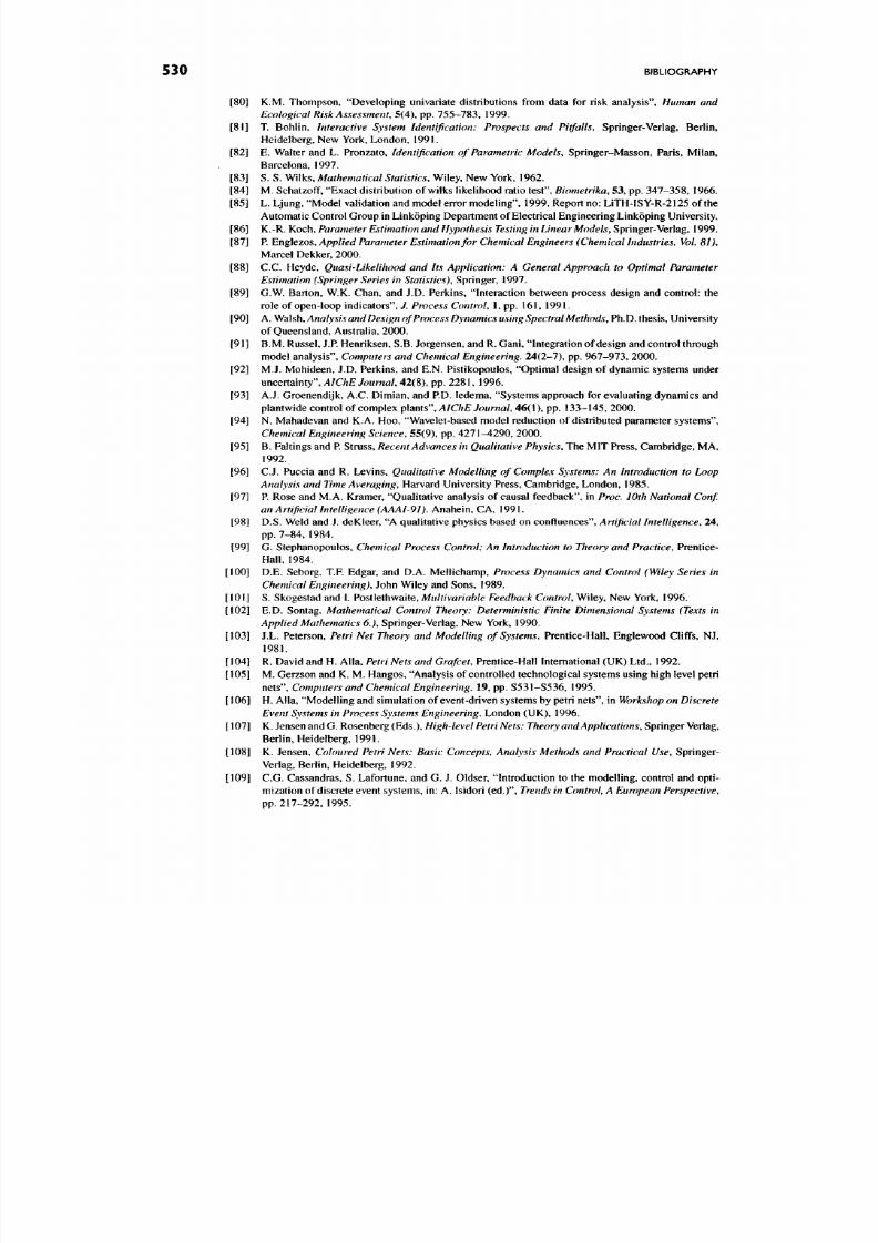
8/17/2019 Process Modelling and Model Analysis-Hangos-Cameron
http://slidepdf.com/reader/full/process-modelling-and-model-analysis-hangos-cameron 547/560
530
BIBLIOGRAPHY
[80 ] K.M. Thompson, "Developing univariate distributions from data for risk analysis", Human and
Ecological Risk Assessment, 5(4), pp. 755 -783 , 1999.
[81] T. Bohlin, Interactive System Identification: Prospects and Pitfalls, Springer-Verlag, Berlin,
Heidelberg, New York, London, 1991.
[82 ] E. Walter and L. Pronzato,
Identification
of
Parametric
Models, Springer-Masson, Paris, Milan,
Barcelona, 1997.
[83] S. S. Wilks, Mathematical Statistics, Wiley, New York, 1962.
[84] M. Schatzoff, "Exact distribution of wilks likelihood ratio test", Biometrika, 5 3, pp. 347-358,1966.
[85 ] L. Ljung, "Model validation and model error modeling", 199 9, Report no: LiTH-ISY-R-2125 of the
Automatic Control Group in L inkoping Department o f Electrical Engineering Linkoping University.
[86 ] K.-R. Koch,
Parameter Estimation
and
Hypothesis Testing in
Linear Models, Springer-Verlag, 1999.
[87] P. Englezos, Applied Parameter E stimation for Chemical Engineers (Chemical I ndustries, Vol. 81),
Marcel Dekker, 2000 .
[88] C.C. Heyde,
Quasi-Likelihood and I ts Application: A G eneral Approach to O ptimal Parameter
Estimation (Springer
Series in Statistics), Springer, 1997.
[89] G.W. Barton, W.K. Chan, and J.D. Perkins, "Interaction between process d esign and control: the
role of open-loop indicators", 7. Process
Control,
1, pp. 161, 1991.
[90] A. Walsh,
Analysis and Design of Process Dynamics using Spectral Methods,
Ph.D.
thesis. U niversity
of Queensland, Australia, 2000.
[91] B.M. Russel,
J.P.
Henriksen, S.B. Jorgensen, and R. Gani, "Integration of design and control through
model analysis". Computers a nd Chemical Engineering. 24(2-7), pp. 967-973, 2000.
[92] M.J. Mohideen, J.D. Perkins, and E.N. Pistikopoulos, "Optimal design of dynamic systems under
mcerimnty , AIChE
Journal, 42(8), pp. 2281, 1996.
[93] A.J. Groenendijk, A.C . Dimian, and P.D. ledema, "Systems approach for evaluating dynamics and
plantwide control of complex plants", AIChE
Journal,
46(1), pp. 133-145, 2000.
[94 ] N. Mahadevan and K. A. H oo, "Wavelet-based model reduction of distributed parameter systems",
Chemical Engineering Science, 55(9), pp. 4271 -4290 , 2000.
[95 ] B. Faltings and P. Struss, Recent Advances in Qu alitative Physics, The MIT Press, Cambridge, MA,
1992.
[96 ] C.J. Puccia and R. Levins, Qualitative Modelling of Complex Systems: An Introduction to Loop
Analysis and Time Averaging, Harvard University Press, Cambridge, London, 198 5.
[97 ] P. Rose and M.A. Kramer, "Qualitative analysis of causal feedback", in Pwc. lOth National Conf.
an A rtificial Intelligence (AAAI-9I) . Anahein, CA, 1991.
[98 ] D.S. Weld and J. deKleer, "A qualitative physics based on confluences". Artificial Intelligence, 24,
pp.
7-84, 1984.
[99 ] G. Stephanopoulos, Chemical Process Control: An
Introduction
to
Theory
and Practice, Prentice-
Hall, 1984.
[10 0] D.E. Seborg, T.F. Edgar, and D.A. Mellichamp, Process Dynam ics and C ontrol (W iley Series in
Chemical E ngineering), John Wiley and Sons, 1989.
[10 1] S. Skogestad and I. Postlethwaite, Mu ltivariable Feedback
Control,
Wiley, New York, 1996.
[102] E.D. Sontag, Mathem atical Control Theory: Deterministic Finite Dimensiona l Systems (Texts in
Applied Mathematics 6.), Springer-Verlag, New York, 1990.
[10 3] J.L. Peterson,
Petri Net Theory and Modelling of Systems,
Prentice-Hall, Englewood Cliffs, NJ,
1981.
[104] R. David and H. Alia, Petri Nets and
Grafcet,
Prentice-Hall International (UK) Ltd., 1992.
[10 5] M. Gerzson and K. M. Hangos, "Analysis of controlled technological systems using high level petri
nets", Computers
a nd
Chemical
Engineering, 19, pp. S531 -S536, 1995.
[10 6] H. Alia, "Modelling and simulation of event-driven systems by petri nets", in Workshop on Discrete
Event Systems in Process Systems Engineering. London (UK), 1996.
[ 107] K. Jensen and G. Rosenberg (Eds.), High-level Petri Nets: Theory and Applications, Springer Verlag,
Beriin, Heidelberg, 1991.
[10 8] K. Jensen, Coloured Petri Nets: B asic Concepts, Analysis Methods and Practical Use, Springer-
Veriag, Beriin, Heidelberg, 1992 .
[109] C.G. Cassandras, S. Lafortune, and G. J. Oldser, "Introduction to the mo delling , control and opti
mization of discrete event system s, in: A. Isidori (ed.)".
Trends in
Control, A
European
P erspective,
pp. 217-292, 1995.

8/17/2019 Process Modelling and Model Analysis-Hangos-Cameron
http://slidepdf.com/reader/full/process-modelling-and-model-analysis-hangos-cameron 548/560
BIBLIOGRAPHY 531
[11 0] R. David and H. Alia, "Petri nets for modelling of dynamic systems— a survey", Automatica, 30,
pp. 175-202, 1994.
[ I l l ]
P.
P hilips, K.B. Ramkumar,
K.W. Lim,
H. A. Preisig,
and M.
Weiss, "Automaton-based fault detection
and isolation". Computers and Chemical Engineering, 23, pp. S215 -S218 , 1999.
[11 2] A. Sanchez, G. Rotstein, N. Alsop, and S. Machietto, "Synthesis and implementation of procedural
controllers for event-driven operdAiom'\ AIChE
Journal,
45, pp. 1753-1775 , 1999.
[11 3] T. Nishi, A . Sakata, S. Hasebe, and I. Hashimo to, "Autonomous decentralized scheduling system
for just-in-time production",
Computers
a nd
Chemical Engineering,
24, pp. 345 -35 1, 2000.
[114] C. Azzaro-Pantel, L. Bemal-Haro,
P.
Bauder, S. Dom enech,
and L.
Pibouleau,
"A
two-stage method
ology for short-term batch plant scheduling: Discrete event simulation and genetic algorithm",
Computers a nd Chemical Engineering, 22, pp. 1461-14 81,1998.
[11 5] S. Viswanathan, C. Johnsson, R. Srinivasan, V. Venkatasubramanian, and K.E. Arzen, "Automating
operating procedure synthesis for batch processes: Part I. knowledge representation and planning
framework". C omputers and
Chemical
Engineering, 22, pp. 1673-1685, 1998.
[11 6] S. Viswanathan, C. Johnsson, R. Srinivasan, V. Venkatasubramanian, and K.E. Arzen, "Automat
ing operating procedure synthesis for batch processes: Part II. implementation and application".
Computers a nd Chemical Engineering, 22, pp. 1687-1698, 1998.
[11 7] R. Srinivasan and V. Venkatasubramanian, "Automating hazop analysis for batch chemical plants:
Part i. the knowledge representation framework". Computers and C hemical En gineering, 22,
pp.
1345-1355, 1998.
[11 8] R. Srinivasan and V. Venkatasubramanian, "Automating hazop ana lysis for batch chemical plants:
Part II. algorithms and application". Computers and Chemical Engineering, 22, pp. 1357-1370,
1998.
[11 9] A. Szucs , M. Gerzson, and K.M. Hango s, "An intelligent diagnostic system based on Petri nets".
Computers and Chem ical Engineering, 22, pp. 1335-1344, 1998.
[12 0] S. Gonnet and O. Chiotti, "Modelling of the supervisory control system of a multi-purpose batch
plant". Com puters and Chemical Engineering, 23, pp. 611 -622 , 1999.
[12 1] B. Lennartson, B. Egardt, and M. Tittus, "Hybrid systems in process control", Proc. 33rd CDC, 4,
pp.
3587-3592, 1994.
[12 2] S. Petterson and B. Lennartson, "Hybrid modelling focussed on hybrid Petri nets",
2n d European
Workshop on Real-time and Hybrid Systems, 1995.
[12 3] T.A. Henzinger, P.-H. Ho, and H. Wong-Toi, "Algorithmic analysis of nonlinear hybrid systems",
IEEE Transactions
on
Automatic
Control, 43(4), pp. 540 -554 , 1998.
[12 4] V.D. Dimitriadis, N. Shah, and C.C. Pantelides, "Modelling and safety verification of dis
crete/continuous processing systems , AIChE
Journal,
34(4), pp. 1041 -1059,1997.
[12 5] Process Systems Enterprise Ltd., "gPROMS", 200 0, http://www.psenterprise.com/products/
products.html.
[126] Daesim Technologies, "Daesim Studio", 200 1, http://www.daesim.com/.
[127] E. Hairer, S.P. N0rsett, and G. Wanner, Solving O rdinary Differential Equations, Springer-Verlag,
Berlin, 1991.
[12 8] VR . Marshall M.J. Hounslow, R.L. Ryall, "A discretized population balance for nucleation, growth
and ag gregation", AIChEJ, 34(11), pp. 182 1-1832,1988.
[ 129] E.
Hairer
and G.
Wanner,
Solving Ordinary Differential Equations
II :
Stiffand D ifferential-Algebraic
Problems, Springer-Verlag, 1996.
[13 0] H.A. Preisig, "A mathematical approach to discrete-event dynamic modelling of hybrid systems".
Computers and Chemical Engineering, 20, pp. SI301- SI306, 1996.
[13 1] G. Schilling and C.C. Pantelides, "Optimal periodic scheduling of multipurpose
plants",
Com puters
an d
Chemical
Engineering, 23, pp. 635-655 ,1999 .
[13 2] K. Wang, T. Lohl, M. Stobbe, and S. Engell, "Optimal periodic scheduling of multipurpose plants",
Computers and Chemical Engineering, 24, pp. 39 3^ 00 , 2000.
[13 3] O. Abel and W. Marquardt, "Scenario-integrated m odelling and optimization of dynamic systems",
AIChE
Journal, 46(4), pp. 803 -823 , 2000.
[134] AusIMM, A Comprehensive Dynamic Model of the Pierce-Smith Copper C onverter: A F irst Step
Towards Better Converter-Aisle O peration, Mount Isa, 1 9-23 April 1998.
[ 135] S. Goto, "Equilibrium calculations between matte, slag and gaseous phases in copper
making,
copper
metallurgy practice and theory", IMM, pp. 23-34, 1974.

8/17/2019 Process Modelling and Model Analysis-Hangos-Cameron
http://slidepdf.com/reader/full/process-modelling-and-model-analysis-hangos-cameron 549/560
532
BIBLIOGRAPHY
[136]
[137]
[138]
[139]
[140]
[141]
[142]
[143]
[144]
[145]
[146]
[147]
[148]
[149]
[150]
[151]
[152]
[153]
[154]
[155]
[156]
[157]
[158]
[159]
[160]
[161]
[162]
[163]
[164]
R.Williams and
S.
Pickering, "Modelling the UV light reactor rig" , 1998, El 870 Report, Department
of Chemical Engineering, The University of Queensland.
E. Von Munch,
Mathematical Modelling of
Prefermenters, Ph.D. thesis. Department of Chemical
Engineering, The University of Queensland, 1997.
A. Adetayo, J.D. Litster, and M. Desai, "The effect of process parameters on drum granulation of
fertilizers with broad size distributions". Chemical Engineering Science, 48(23), pp. 3951-3961,
1993.
J.D. Litster, FY. Wang, I.T. Cameron, and RL. Douglas, "A distributed parameter approach to the
dynamics of rotary drying processes", Drying Techn., 11(7), pp. 1641 -1656, 1993.
G.C. Brasil and M.M. Seckler, "A model for the rotary drying of granulator fertilisers", Pivc. 6th
Int. Drying Symp., pp. 247-256, 1988.
S.J. Friedman and W.P. Mashell, "Studies in rotary drying, parts 1 and 2",
Chem. Eng. Prog.,
45,
889,
pp. 482-493 and 573-588 , 1949.
W.J. Whiten, Simulation and Model Building for Mineral Processing, PhD thesis, University of
Queensland, Australia, 1972.
A.J. Lynch, Mineral Crushing and Grinding Circuits, Elsevier Scientific, New York, 1977.
LT.
Cameron and FY. Wang, "Dyn amics of fractionators with structured packin g",
Chem.Eng.Commun.,
119, pp. 231-259 , 1993.
M. Sadeghi, Dynamic Modelling and Simulation of Structured Packing Fractionators, PhD thesis.
University of Queensland, Brisbane, Australia, 1996.
H. Takenchi, K. Ond a and Y. Oku moto , "Ma ss transfer coefficients b etween gas and liquid in packed
beds", J. Chem. Eng. Japan,
1(1), pp. 56 -62 , 1968.
J.A. Rocha, J.L. Bravo, and J.R. Fair, "Mass transfer in gauze packings",
Hydroc. Proc,
64(1),
p p . 9 1 -9 5 ,
1985.
L. Spiegel and W. Meier, "Correlations of the performance characteristics of various mellapak types",
Inst.
Chem. Engrs. Symp. Sen, 104, pp. A20 3-A2 15, 1987.
R. Billet, "Modelling of fluid dynamics in packed columns",
IChemE Symp. Ser.,
104, pp. A171,
1987.
J.R. Fair, J.L. Bravo, and J.A. Rocha, "A comprehensive model for the performance of columns
containing structured packing ",
AIChemE Symp. Ser,
128, pp. A439, 1992.
Aspen Technology Inc., "ASPEN PLU S", 2000, http://www.aspentech.com/.
Hyprotech Ltd, "HYSYS integrated simulation for the continuous processing industries", 2000,
http://www.hyprotech.com/products/.
Mathworks Inc, "MATLAB software system", 2 001 , http://www.mathworks.com/.
W. Marquardt, "Trends in com puter-aided modeling". Computers and Chemical Engineering, 20,
pp .
591-609, 1996.
Anne Krogh Jensen, Generation of Problem Specific Simulation Models
Within
an In tegrated
Computer Aided System, PhD thesis, Danish Technical University, 1998.
B. Lohmann, B.A. Foss, and W. Marquardt, "A field study of the industrial modeling process".
Journal of Process Control, 5, pp. 325 -338, 1998.
JKTech
Ltd,
"SimM et—simulator for minerals processing circuits", 2001, http://www.jktech.com.au/.
CAPE-OPEN, "Global CAPE-OPEN (GCO) standards in computer-aided process engineering",
2000,
http://www.global-cape-open.org/.
H.A. Preisig, "Modeller—an object oriented computer-aided modelling tool", in 4th International
Conference on the Foundations of Computer-Aided Process Design. 1995, pp. 328-331, CACHE
Corporation, U SA.
ModKit, "Computer aided process modeling (ModKit)", 2000, http://www.lfpt.rwth-aachen.de/
Research/Mod el ing/modkit, html.
G. Stephanopoulos, G. Henning, and H. Leone, "MODEL.LA a modeling language for process
engineering—1 the formal framework". Computers and Chemical Engineering, 8, pp. 813-846,
1990.
K.M. Hangos, R. Williams, and I.T. Cameron, "Assumption structures for model building", Tech.
Rep.
091299, CAPE Centre, The University of Queensland, 1999.
H. Rittel and W. Kunz, "Issues as elements of information sy stems" . Tech. Rep. Working Paper 131,
Institute of Urban and Regional Development, University of California, Berkeley, CA, 1970.
R. Banares-Alcantara and H.M.S. Lababidi, "Design support systems for process engineering: 1
and".
Computers
a nd
Chemical
Engineering, 19, pp. 267 -301 , 1995.
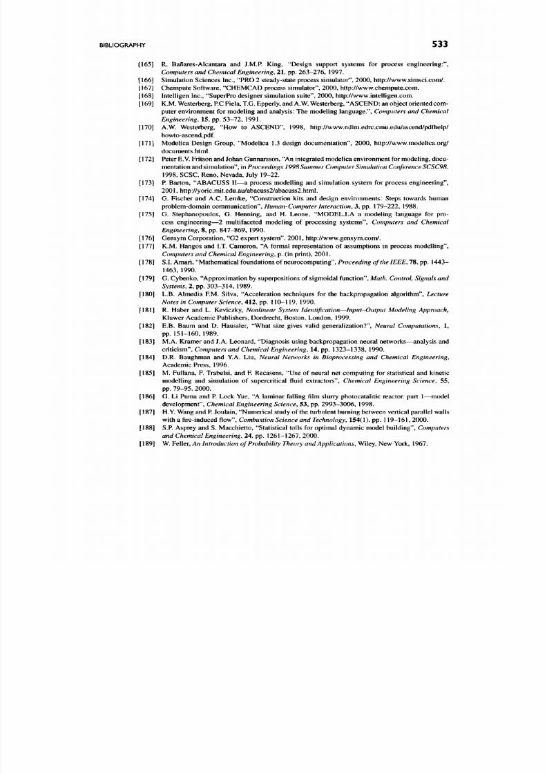
8/17/2019 Process Modelling and Model Analysis-Hangos-Cameron
http://slidepdf.com/reader/full/process-modelling-and-model-analysis-hangos-cameron 550/560
B I B L I O G R A P H Y 5 3 3
[16 5] R. Baiiares-Alcantara and J.M.P. King, "Design support systems for process engineering:".
Computers and Chemical Engineering,
21, pp. 263-276, 1997.
[16 6] Simulation Sciences Inc., "PRO 2 steady-state process simulator", 200 0, http://www .simsci.com /.
[16 7] Chempute Software, "CHEMCAD process simulator", 20 00, http://www.chemp ute.com.
[16 8] Intelligen Inc., "SuperPro designer simulation suite", 200 0, http://www.intelligen.com.
[16 9] K.M. Westerberg, PC Piela, T.G. Epperly, a n d A . W . Westerberg, "ASCE ND: an object oriented com
puter environment for modeling and analysis: The modeling language.". Com puters and Chemical
Engineering, 15, pp. 53 -72 , 1991.
[17 0] A.W. Westerberg, "How to ASC END ", 1998, http://www .ndim.edrc.cmu.edu/ascend/pdfhelp/
howto-ascend.pdf.
[17 1] Mod elica Desig n Group, "Modelica 1.3 design documentation", 20 00 , http://www.mo delica.org/
documents.html.
[ 172] Peter
E . V .
Fritson
a n d
Johan Gunnarsson,
A n
integrated modelica environment for modeling, docu
mentation and simulation", in
Proceedings 1998 Summer C omputer Simulation
Conference
SCSC98.
1 9 9 8 , SCSC, Reno, Nevada, July 19-2 2.
[17 3] P. Barton, "ABAC USS II—a process modelling and simulation system for process engineering",
2 0 0 1 , http://yoric.mit.edu.au/abacuss2/abacuss2.html.
[17 4] G. Fischer and A.C. Lemke, "Construction kits and design environments: Steps towards human
problem-domain communication",
Human-Computer Interaction,
3, pp. 179-22 2, 1988.
[17 5] G. Stephanopoulos, G. Henning, and H. Leone, "MODEL.LA a modeling language for pro
cess engineering—2 multifaceted modeling of processing systems", Computers and Chemical
Engineering, 8, pp. 847 -869 , 1990.
[17 6] Gensym Corporation, "G2 expert system", 20 01 , http://www.gensy m.com /.
[17 7] K.M. Hangos and I.T. Cameron, "A formal representation of assumptions in process modelling",
Computers and Chemical Engineering, p. (in print), 200 1.
[ 178] S.I. Amari, "Mathematical foundations of neurocomputing". Proceeding of t h e IEEE, 7 8, p p . 1443-
1 4 6 3 , 1990.
[17 9] G. Cybenko, "Approximation by superpositions of sigmoidal function". Math. Control,
Signals and
Systems, 2, pp. 303 -314 , 1989.
[18 0] L.B. Alm edia F.M. Silva, "A cceleration techniques for the backpropagation algorithm".
Lecture
Notes in Computer Science, 412, pp. 110-119, 1990.
[181] R. Haber and L. Keviczky,
Nonlinear System Identification
—
Input-Output Modeling Approach,
Kluwer Academic Publishers, Dordrecht, Boston, London, 1999.
[18 2] E.B. Baum and D. Haussler, "What size gives valid generalization?". Neural Computations, 1,
p p . 151-160, 1989.
[18 3] M.A. Kramer and J.A. Leonard, "Diagnosis using backpropagation neural networks— analysis and
criticism", Computers and Chemical Engineering, 14, pp. 1323-1338, 1990.
[184] D.R. Baughm an and Y.A. Liu,
Neural Networks in Bioprocessing and Chemical Engineering,
Academic Press, 1996.
[18 5] M. Fullana, F. Trabelsi, and F. Recasens, "U se of neural net computing for statistical and kinetic
modelling and simulation of supercritical fluid extractors", Chem ical E ngineering Science, 55,
p p . 79-95, 2000.
[186] G. Li Puma and P. Lock Yue, "A laminar falling film slurry photocatalitic reactor, part
1—model
development". Chemical Engineering Science, 53, pp. 2993 -3006 , 1998.
[ 187] H. Y . Wang and P . Joulain, "Numerical study of th e turbulent burning between vertical parallel walls
with a i r e - i n d u c e d flow ,
Combustion Science and Technology,
154(1), pp. 119-16 1, 2000.
[18 8] S.P. Asprey and S. Macchietto, "Statistical tolls for optimal dynamic model building". C omputers
and Chemical Engineering,
24 , pp. 1 261-1267, 2000.
[189] W. Feller, An Introduction of Probab ility Theory and Applications, Wiley, New York, 1967.

8/17/2019 Process Modelling and Model Analysis-Hangos-Cameron
http://slidepdf.com/reader/full/process-modelling-and-model-analysis-hangos-cameron 551/560

8/17/2019 Process Modelling and Model Analysis-Hangos-Cameron
http://slidepdf.com/reader/full/process-modelling-and-model-analysis-hangos-cameron 552/560
INDEX
7 Step modelling procedure, see
seven step modelling procedure
A/D converter,
s ee
sampling
Adams method, see num erical
methods for solving ODEs
AI, see artificial intelligence
AI models,
see
qualitative models
Algebraic equation set
assignment of, 153
digraph of, 154
incidence matrix of, 153
Algorithm
for lumping distributed parameter
models, 185
for the solution of finite automata
models, 405
for the solution of Petri net
models, 395, 407
Algorithmic complexity, 253, 390
of analysis of structural stability,
348
of analysing discrete event system
models, 408
of the solution of Petri net models,
397
of validating rule-sets, 380
Alphabet, see finite automata model
Alternating-direction implicit (ADI)
method, s ee numerical methods
for solving PDEs
Analysis of discrete event system
models, 408-410
algorithmic complexity of, 408
behavioural p roperties, 408
conflict situations, 410
deadlocks, 409
finiteness, 40 9
invariance (structural) properties,
408
reachability (controllability), 409
Analysis of dynamic process models,
335-350
(state) controllability, 338
(state) observability, 336
stability, 340
Analysis of lumped parameter
models, 104-117
degrees of freedom (DOF), 104
dynamical properties, see
dynamical properties
factors leading to high index, 111
ill-conditioning, 113
in CAPM tools, 480
index, 108
stability, 113
stiffness, 113, 116
structural dynam ical properties,
see
structural dynamical
properties
Application examples, 437-470
copper converter, s ee copper
converter
depropanizer,
see
depropanizer
granulation circuit, s ee granulation
circuit
phenol destruction, s ee phenol
destruction
prefermenter,
see
prefermenter
wastewater treatment, see
wastewater treatment
ARMAX model, 505-507, 512
Artificial intelligence, 372
ASCEND
in CAPM tools, 485
Assignment
in a structure matrix, 342
of an algebraic equation set, 153
Assumptions, s ee modelling
assumptions
Asymptotic (internal) stability, see
dynamical properties
Automata,
see
finite automata model
hybrid, see hybrid automata
Backward chaining, see reasoning
Backward differentiation formula
(BDF), see numerical methods
for solving OD Es
Backward Euler method, see
numerical methods for solving
ODEs
Balance equation, s ee conservation
balances
differential, in operator form, 55
flow term, 52
in rectangular co-ordinate system,
56
source term, 53
transport term, 52
Balance violation, s ee data screening
Balance volumes, 58-60, 7 5
distributed parameter models, 165
distributed, in different co-ordinate
system, 165
in CAPM tools, 475
in model hierarchies, 231, 238,
244
infinitely large, 172
535

8/17/2019 Process Modelling and Model Analysis-Hangos-Cameron
http://slidepdf.com/reader/full/process-modelling-and-model-analysis-hangos-cameron 553/560
536
INDEX
Balances, se e conservation balances
Behavioural properties
of discrete event system models,
se e
analysis of discrete event
system models
BIBO stability,
see
dynamical
properties
Black-box
functional relationship, 496
model element, 495
model simplification (reduction),
355
Black-box model, 23, 300, 493-515
Boundary conditions
Dirichlet (first type), 170
false boundary approach, 200
Neumann (second type), 171
of distributed parameter models,
170
of elliptic PDEs, 184
ofPDEs, 170
Robbins (third type), 171
virtual, 171
Boundary value problem (BVP), see
distributed parameter models
Bounded-input bounded-output
(BIBO) stability, s ee dynamical
properties
BVP, see boundary value problem
CAPE-OPEN initiatives, 473
CAPM tools, 471-492
ASCEND, 485
balance volumes, 475
Daesim Studio, 491
decision support systems, 482
flowsheet modelling environment,
484
general modelling languages, 484
gPROMS, 486
graphical user interface (GUI), 486
IBIS,481
ModDev, 490
model analysis, 480
model documentation, 480
model hierarchies, multi-level, 477
model hierarchies, mu lti-scale, 478
model solution, 480
ModeUaASl
Modelica, 486
modelling goal, 483
modelling structures, 474
ModKit, 489
process knowledge based
environments, 487
simulation, 482
Characteristic po lynomial, 365
Circle (directed), see digraph
Circle families
in analysing structural stability,
348
Circle families (directed), see signed
directed graph (SDG)
Co-ordinate system
cylindrical, 43, 168
for distributed parameter models,
165
rectangular, 43
spherical, 43, 168
Coloured Petri nets (CPNs), see Petri
net model
Completeness
of a rule set, 382
of discrete event system models,
see discrete event system
models
Computational fluid dynamics
(CFD), 472
Computer aided process mod elling,
see
CAPM tools
Conflict situation
in a Petri net, 396
of discrete event systems,
see
analysis of discrete event
system models
Confluences, 378-380
application of, 379
generation of rules from, 380, 382
operation (truth) table of, 379
solution of, 379
Conservation
balances,
see
conservation
balances
matrix,
s ee
conservation matrix
principle of, 51-58
Conservation balances
differential form, 52, 164
differential, in operator form, 55,
168
distributed, see distributed
conservation balances
in rectangular co-ordinate system,
56
integral form, 51
lumped,
s ee
lumped conservation
balances
of a copper converter, 441
of a depropanizer, 464
of a granulation circuit, 458
of a prefermenter, 453
of phenol destruction, 447
Conservation matrix, 345,348
Consistency
of a rule set, 382
Constitutive equations, 65-79
of a depropanizer, 465
of phenol destruction, 449
potential variable relations, 54
reaction rate equations, 70
thermodynamical relations, see
thermodynamical relations
transfer rate equations,
see
transfer
rate equations
Constitutive relations, see
constitutive equations
Control algebraic Ricatti equation,
367
Control gain, 364
Controllability (state controllability),
see
dynamical properties
in pole-placement c ontrol, 365
of discrete event systems, see
analysis of discrete event
system models
structural,
s ee
structural
controllability
Controllers
for process systems,
see
process
control
full state feedback controllers,
365, 367
linear quadratic regulator (LQ R),
366
model-based predictive control,
368
pole-placement control, 365
proportional (P) control, 78
proportional-integral (PI) control,
79
proportional-integral-derivative
(PID) control, 79
Controlling factor, see controlling
mechanism
Controlling mechanism, 2 6
of a copper converter, 439
of a depropanizer, 462
of a granulation circuit, 457
of a prefermenter, 452
of phenol destruction, 445
Copper converter, 438-443
conservation balances, 441
controlling m echanism, 439
modelling assumptions, 440
modelling goal, 438
particle population balance, 4 42
process description, 43 8
Correlation coefficient, 312, 327
Covariance matrix
in LS parameter estimation, 308
CPN, see Petri net models, coloured
Crank-Nicholson implicit method,
see
numerical methods for
solving PDEs
CUSUM method, s ee data screening
D/A converter, see sampling
DAE set, s ee DAE systems
DAE systems, 84, 123
algebraic equation set, see
algebraic equation set
high index, 108
hybrid, s ee hybrid DAE systems
index, 108
initial value (DAE-IVP) problem,
99
numerical solution, 149-155
Daesim Studio

8/17/2019 Process Modelling and Model Analysis-Hangos-Cameron
http://slidepdf.com/reader/full/process-modelling-and-model-analysis-hangos-cameron 554/560
INDEX
537
in CAPM tools, 491
Damkohler number, 103
Data
acquisition and analysis, 285-296
screening, s ee data screening
visualization, 290
Data screening, 289-294
balance violation detection, 293
CUSUM method, 292
data visualization, 29 0
gross error detection, 293
jump detection, 293
outlier test, 292
simple statistics, 290
steady-state test, 292
trend detection, 292
Deadlocks
of discrete event systems, see
analysis of discrete event
system models
Decision support systems
in CAPM tools, 482
Degrees of freedom
analysis for lumped parameter
models, 104
independent intensive quantities,
50
selecting variables to satisfy it, 105
Depropanizer, 462-469
conservation balances, 46 4
constitutive equations, 4 65
controlling mechanism, 462
model validation, 468
modelling assumptions, 463
packed column section, 464
process description, 462
Design variables, 106
Diagnosis (process diagnosis),
370-372
identification-based diagnosis, 371
prediction-based diagno sis, 370
Diagonally implicit Runge-Kutta
method, s ee numerical methods
for solving OD Es
Digraph
bip£irtite, 394
of a finite automata (state
transition g raph), 390
of an algebraic equation set, 154
of an LTI system model, 279
of Petri net structure, 394
strong component, 154
Dimensionless variables, 101
Dirac delta function,
see
special test
signals
Directed graph, s ee digraph
Dirichlet boundary conditions,
see
boundary conditions
DIRK method, see diagonally
implicit Runge-Kutta method
Discrete event simulation,
see
discrete event system models
Discrete event system models,
387-410
analysis of,
see
analysis of d iscrete
event system models
as dynamic system models, 402
as qualitative m odels, 388
completeness, 403
discrete event simulation, 404
event, 387, 388
exception handling, 403
external events, 388
finite automata models, see finite
automata model
internal events, 388
Petri net models, see Petri net
model
solution of, 404
state change, 395
Distributed c onservation balances,
165
in cylindrical co-ordinate system,
168
in spherical co-ordinate system,
168
of a rotary drier, 459
of an UV reactor, 448
Distributed parameter models,
163-186
balance volumes, 165
boundary conditions,
see
boundary
conditions
classification, 182
co-ordinate system, 165
conservation balances, 165
domain, 170, 184
effect of steady-state assumption,
184
examples of heat transfer, 174
examples of reaction engineering,
178
finite difference approximation,
185
initial conditions, 173
lumping, 185,201,227
modelling assumptions leading to
model classes, 184
modelling assumptions, boundary
conditions, 171
modelling assumptions, model
equations, 174
origin of, 164
solution strategies, 191-218
well-posed, 171
Disturbace variables,
s ee
systems
DOF,
see degrees of freedom
Domain
of distributed parameter models,
see distributed parameter
models
of elliptic PDEs, 184
DPS models,
see
distributed
parameter models
Dynamic models
discrete event, described by timed
Petri nets, 398
distributed parameter, see
distributed parameter models
experiment design for parameter
estimation, 295
lumped parameter, see lumped
parameter models
lumped p redictive parametrized
discrete time, 369-371
lumped, analysis of, see analysis
of dynamic process models
lumped, structural analysis of,
see
structural dynamical
properties
of a copper converter, 438
of a depropanizer, 462
of a granulation circuit, 455
of a phenol destruction process,
443
of a prefermenter, 450
of discrete event systems, 402
Dynamical properties, 335-350
asymptotic (internal) stability, 340
asymptotic stability of LTI
systems, 341
BIBO stability of LTI systems, 340
bounded input bounded output
(BIBO) stability, 340
controllability (state
controllability), 338
controllability of LTI systems, 338
observability (state observability),
336
observability of LTI systems, 336
realization property, 337, 339
structural, s ee structural dynamical
properties
system property, 339-341
Empirical model, 10
building of,
see
black-box model
Empirical variance, see sample, 327
Equipment and control relations,
75-79
actuators, 77
control valves, 78
controllers, s ee con trollers
sensors, 76
transmitters, 77
Estimate
in model parameter estimation,
303
quality of, 303
Euler*s method,
s ee
numerical
methods for solving ODEs
Event, s ee discrete event system
models
Exception handling
using discrete event system
models, 403
Excitation, s ee experiment design
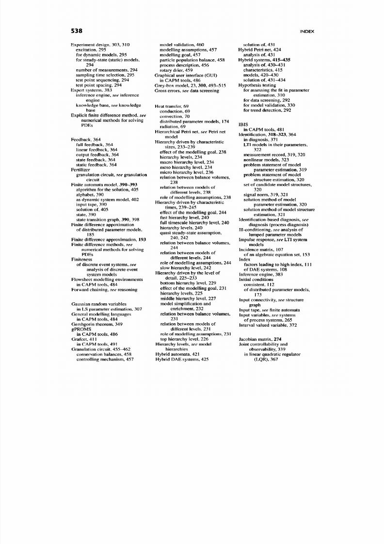
8/17/2019 Process Modelling and Model Analysis-Hangos-Cameron
http://slidepdf.com/reader/full/process-modelling-and-model-analysis-hangos-cameron 555/560
538
INDEX
Experiment design, 303, 310
excitation, 295
for dynamic models, 295
for steady-state (static) models,
294
number of measurements, 294
sampling time selection, 295
test point sequencing, 294
test point spacing, 294
Expert systems, 383
inference engine, s ee inference
engine
knowledge base, see knowledge
base
Explicit finite difference method, see
numerical methods for solving
PDEs
Feedback, 364
full feedback, 364
linear feedback, 364
output feedback, 364
state feedback, 364
static feedback, 364
Fertilizer
granulation circuit,
s ee
granulation
circuit
Finite automata model, 390-393
algorithm for the solution, 405
alphabet, 390
as dynamic system model, 402
input tape, 390
solution of, 405
state, 390
state transition graph, 390, 398
Finite difference appoximation
of distributed parameter models,
185
Finite difference approximation, 193
Finite difference methods, see
numerical methods for solving
PDEs
Finiteness
of discrete event systems, see
analysis of discrete event
system models
Flowsheet m odelling environments
in CAPM tools, 484
Forward chaining, s ee reasoning
Gaussian random variables
in LS parameter estimation, 307
General modelling languages
in CAPM tools, 484
Gershgorin theorem, 349
gPROMS
in CAPM tools, 486
Grafcet, 411
in CAPM tools, 491
Granulation circuit, 455-462
conservation balances, 458
controlling mechanism, 457
model validation, 460
modelling assumptions, 457
modelling goal, 457
particle population balance, 45 8
process description, 456
rotary drier, 459
Graphical user interface (GUI)
in CAPM tools, 486
Grey-box model, 23, 300, 493-515
Gross errors, see data screening
Heat transfer, 69
conduction, 69
convection, 70
distributed parameter models, 174
radiation, 69
Hierarchical Petri net,
see
Petri net
model
Hierarchy driven by characteristic
sizes,
233-239
effect of the modelling goal, 238
hierarchy levels, 234
macro hierarchy level, 234
meso hierarchy level, 234
micro hierarchy level, 236
relation between balance volumes,
238
relation between models of
different levels, 238
role of modelling assumptions, 238
Hierarchy driven by characteristic
times, 239-245
effect of the modelling goal, 244
fast hierarchy level, 240
full timescale hierarchy level, 240
hierarchy levels, 240
quasi steady-state assumption,
240,
242
relation between balance volumes,
244
relation between models of
different levels, 244
role of modelling assumptions, 244
slow hierarchy level, 242
Hierarchy driven by the level of
detail, 225 -233
bottom hierarchy level, 229
effect of the modelling goal, 231
hierarchy levels, 225
middle hierarchy level, 227
model simplification and
enrichment, 232
relation between balance volumes,
231
relation between models of
different levels, 231
role of modelling assumptions, 231
top hierarchy level, 226
Hierarchy levels, se e model
hierarchies
Hybrid automata, 421
Hybrid DAE systems, 425
solution of, 431
Hybrid Petri net, 424
analysis of, 431
Hybrid systems, 415-435
analysis of, 430 -431
characteristics, 415
models, 420-43 0
solution of, 431-434
Hypothesis testing
for assessing the fit in parameter
estimation, 310
for data screening, 292
for model validation, 330
for trend detection, 292
IBIS
in CAPM tools, 481
Identification, 318-323, 364
in diagnosis, 371
LTI models in their parameters,
322
measurement record, 319, 320
nonlinear models, 323
problem statement of model
parameter estimation, 319
problem statement of model
structure estimation, 320
set of candidate model structures,
320
signal norm, 319, 321
solution method of model
parameter estimation, 320
solution method of model structure
estimation, 321
Identification-based diagnosis, see
diagnosis (process diagnosis)
Ill-conditioning,
s ee
analysis of
lumped parameter models
Impulse response,
see
LTI system
models
Incidence matrix, 107
of an algebraic equation set, 153
Index
factors leading to high index, 111
of DAE systems, 108
Inference engine, 383
Initial conditions
consistent, 112
of distributed parameter models,
173
Input connectivity,
s ee
structure
graph
Input tape, see finite automata
Input variables, see systems
of process systems, 265
Interval valued variable, 372
Jacobian matrix, 274
Joint controllability and
observability, 339
in linear quadratic regulator
(LQR), 367
8/17/2019 Process Modelling and Model Analysis-Hangos-Cameron
http://slidepdf.com/reader/full/process-modelling-and-model-analysis-hangos-cameron 556/560
INDEX
539
Jumps in data
data screening, 293
Kalman filter, see process control
Knowledge base, 383
Least squares parameter estimation,
see LS parameter estimation
Legendre polynomials, 205
Levenberg-Marquardt method, see
numerical op timization
Linear
models, see lumped parameter
models
systems, se e systems
Linear and time-invariant systems,
see
LTI systems
Linear multi-step method,
see
numerical methods for solving
ODEs
Linear quadratic regulator (LQ R),
see
process control
Linear transformation
of states in a LTI system model,
262
Linearization,
see
model
linearization
L MM, s ee linear multi-step method
Logical expressions,
s ee
rules
Logical operations, 375, 381
algebraic properties, 375
canonical form, 375
operation table (truth table), 375
Logical variable, 372, 375, 381
Loss function
of model parameter estimation,
302
of model structure estimation, 303
LS parameter estimation, 305-318
assessing the fit, 310
confidence intervals and regions
(nonlinear case), 313
confidence region and intervals
(linear in parameters case),
308
dynamic m odels linear in
parameters, 322
dynamic nonlinear models, 323
estimation method, 306
extension to the vector-valued
linear in parameter case, 306
handling measurement errors, 307
loss function, 3 06, 313
models linear in parameters, 305
nonlinear models, 312
problem statement, linear in
parameter case, 305
properties in linear in parameter
case,
308
signal norm, 305
static models linear in parameters,
317
sum of squares (SOS), 312
weighting matrix, 307
LTI system models, 254, 255-258
asymptotic stability, 341
balanced realization, 3 56
controllability (state
controllability), 338 , 340
discrete time stochastic, 367
dynamic analysis of, 259
impulse response, 256
linear differential equations with
constant coefficients, 255
linear quadratic regulator (LQR),
366
linear static full state feedback,
364
linearized, 274
model reduction, 355
model simplification, 351
observability (state observability),
336
parameters, 258
pole-placement control, 365
sampled, 286
signed directed graph (SDG) of,
377
simple examples, 259
state filtering, 367
state space representation, 2 58
structure graph, 278
structure of, 278, 350, 377
transformation of states, 262
unit step response, 257
Lump,
see
distributed parameter
models
Lumped conservation balances,
85-101
component mass balance in
intensive variable form, 99
mass,
8 6
momentum, 95
normalized, 102
of a copper converter, 441
of a granulation circuit, 458
of a prefermenter, 453
of an UV reactor, 447
of phenol destruction, 447
set of balances, 98
total energy, s ee lumped energy
balance
total mass, 87
Lumped energy balance, 89-95
conductive and radiative flows, 90
convective energy flow, 90
most common form, 95
simplified, 92
total enegy balance, 91
total energy balance, 89
work terms, 91
Lumped parameter models, 83-118
analysis of, see analysis of lumped
parameter models
as nonlinear state space models,
265-270
conservation balances, 85
control of, see process control
diagnosis of,
see
diagnosis
(process diagnosis)
dynamic, 84
dynamic analysis of,
see
analysis
of dynamic process models
example problems for solution,
124
initial value problems (IVPs), 84
linearization, 270
logical version of, 380
modelling problem, 84
representing distributed peirameter
ones,
185
sampling, 286
sensitivity of, see sensitivity of
models
signed version of, 378
solution strategies, 123-155,155
solving ODE models, see
numerical methods for
solving ODEs
steady state, 84, 103
structural dynamic analysis of,
see
structural dynamical
properties
Lumping,
s ee
distributed parameter
models
Marking, s ee Petri net model
Mathematical mo dels, 22
well-posed, 170, 171
Matrix
conservation, s ee conservation
matrices
Gershgorin theorem, 349
Meeui valu e,
se e
random variable
in LS parameter estimation, 308
Measurement error
in LS parameter estimation, 307
in model parameter estimation,
303
Measurement record,
see
identification
Mesh,
s ee
numerical methods for
solving PDEs
Method of c haracterictics, see
numerical methods for solving
PDEs
Method of lines,
se e
num erical
methods for solving PDEs
Method of weighted residuals, see
numerical methods for solving
PDEs
MIMO systems,
see
systems
linear quadratic regulator (LQR),
366
ModDev
in CAPM tools, 490
8/17/2019 Process Modelling and Model Analysis-Hangos-Cameron
http://slidepdf.com/reader/full/process-modelling-and-model-analysis-hangos-cameron 557/560
540
INDEX
Model
application areas, 7
classification, 10,57
general notion, 4
hierarchies, see model hierarchies
reduction,
see
model reduction
simplification, see model
simplification
validation, s ee model validation
verification, 29
Model c alibration, 299-302
conceptual steps, 301
of a prefermenter, 455
Model documentation
in CAPM tools, 480
Model enrichment,
see
also model
simplification
in model hierarchies, 232
Model hierarchies, 223-245
driven by characteristic sizes,
see
hierarchy driven by
characteristic sizes
driven by characteristic times,
see
hierarchy driven by
characteristic times
driven by the level of detail, see
hierarchy driven by the level
of detail
effect of the modelling goal, 231,
238, 244
hierarchy levels, 225, 234, 240
in CAPM too ls, 477, 478
relation between balance volumes,
231 ,238 ,244
role of modelling assumptions,
231 ,238 ,244
Model linearization, 270-278
Model parameter estimation,
302-330
for model validation, 330
loss function, 302
measurement error variance, 294
measurement errors, 303
of dynamic models, see
identification
of phenol destruction, 449
of static models, 314
problem statement, 302
Model reduction, 355-359
and model simplification, 358
balanced realization, 356
LTI state space models, 355
Model simplification, 350-355
and model reduction, 358
effect on structural control
properties, 354
in model hierarchies, 232
of LTI state space models, 351
problem statement, 350
transformations, 351
variable lumping, 351
variable removal, 351
Model structure estimation, 302
loss function, 303
of dynamic models, see
identification
problem statement, 303
Model validation
of a depropanizer, 468
Model validation, 29, 299,330-331
conceptual steps, 330
of a granulation circuit, 460
of a prefermenter, 455
of phenol destruction, 450
Model verification
via analysis of dynamic process
models, 335
Model-based predictive control, see
process control
Modella
in CAPM tools, 487
Modelica
in CAPM tools, 486
Modelling assumptions
for distributed parameter models,
165, 171, 174, 184
for model hierarchies, 231, 238,
244
of a copper converter, 440
of a depropanizer, 4 63
of a granulation circuit, 457
of phenol destruction, 446
quasi steady-state in model
hierarchies, 240, 242
steady-state, effect on distributed
parameter models, 184
Modelling goal, 21
effect of on balance volumes, 58
effect of on input variables, 265
effect of on model hierarchies,
231 ,238 ,244
effect of on process models, 27
effect of on the outpu t variables,
266
in CAPM tools, 483
of a copper converter, 438
of a granulation circuit, 457
of a prefermenter, 452
of phenol destruction, 444
Modelling procedure
real world, 5
seven step, see seven step
modelling procedure
ModKit
in CAPM tools, 489
Multi-scale modelling, 234
Multiple-input multiple-output
systems, see systems
Neumann boundary conditions, see
boundary conditions
Neural net, 503-505
feedforward, 503
poorly trained, 514
Non-dimensional form,
see
normalization
Normalization
balance equations, 102
ofPDEs, 173
variables, 101
Normalized variables, see
dimensionless variables
Numerical methods for solving
DAEs, 149-155
explicit ODE solver, 150
exploiting equation structure, 152
implicit DAE solver, 151
in CAPM tools, 480
partitioning and precedence order,
152
substitute for algebraic variables,
149
Numerical methods for solving
ODEs, 123-149
absolute stability, 134
Adams m ethod, 145, 147
backward differentiation formula
(BDF), 148
backward Euler method, 128, 147
basic concepts, 126
categories of methods, 127
consistency, 132
controlling steplength
automatically, 144, 146
deriving methods, 137, 145
diagonally implicit Runge-Kutta
method, 141
diagonally implicit Runge-Kutta
method, 138
error estimation, 143, 146
error estimation for Runge-K utta
method, 144
Euler's method, 126, 128, 130,
132,135, 147
Explicit methods, 127
Explicit Runge-Kutta method,
138, 139
global error, 130
implicit methods, 128
implicit Runge-Kutta method, 138
in CAPM tools, 480
linear multi-step method, 129,
145-149
local error, 133
local truncation error, 1 29,13 2
multi-step, 128
Runge-Kutta method, 128,
137-145
semi-implicit Runge-Kutta
method, 138
single step, 128
stability definitions, 136
stability of the method, 132, 133
stability region of a one-step
method, 135
stability region of Adams method,
147
stiff problems, 148
8/17/2019 Process Modelling and Model Analysis-Hangos-Cameron
http://slidepdf.com/reader/full/process-modelling-and-model-analysis-hangos-cameron 558/560
INDEX
541
Numerical methods for solving
PDEs, 191-218
alternating-direction implicit
(ADI) method, 199
Crank-Nicholson implicit method,
195
Crank-Nicholson method, 199
error estimation for finite
difference approximation,
193
explicit finite difference method,
193,199
false boundary app roach, 200
finite difference approximation,
193
finite difference mesh, 192 ,198
finite difference mesh for
Crank-Nicholson method,
195
finite difference mesh for
parabolic equations in one
dimension, 193
finite difference methods, 192
in CAPM tools, 480
method of characteristics, 183
method of
lines,
185, 201-202
method of weighted residuals,
202-205
orthogonal collocation, 205-218
orthogonal collocation for
parabolic equations in one
dimension, 216
orthogonal collocation on
elements, 213
orthogonal collocation with
symmetry, 206
orthogonal collocation without
symmetry, 210
parabolic equations in one
dimension, 193
parabolic equations in two
dimensions, 198
stability region for
Crank-Nicholson method,
195
Numerical optimization
for model parameter estimation,
323
for model-based predictive
control, 369
Levenberg-Marquardt method,
313
Observability (state observability),
see
dynamical properties
structural, s ee structural
observability
Occurrence matrix, see incidence
matrix
of a signed directed graph (SD G),
377
ODE
autonomous form, 126
higher order, 125
initial value problem (OD E-IVP),
114,123
numerical solution of,
see
numerical methods for
solving ODEs
problem statement for solution,
125
Operation
logical, see logical operations
sign, s ee sign operations
Operation table
of confluences, 379
of logical operations, 375
of sign operations, 376
Ordinary differential equation,
see
ODE
Orthogonal collocation,
see
numerical methods for solving
PDEs
Orthogonal function series
expansion, 502
trignometrical basis functions, 5 03
wavelets, 503
Outlier, see data screening
Output connectivity,
see
structure
graph
Output variables, se e systems
of process systems, 266
Parameter estimation,
s ee
model
parameter estimation
dynamic models linear in
parameters, 322
dynamic nonlinear models, 323
static models linear in parameters,
315
static nonlinear m odels, 317
Partial differential equation, s ee PDE
Particle population balance
of a copper converter, 442
of a granulation circuit, 458
Particulate systems
balance equation, 54
Path (directed),
see
digraph
in analysing input and output
connectivity, 345
PDE
boundary conditions, 170
classification of the equations, 182
dispersion convection problem,
202
hyperbolic, 183
normalization, 173
numerical solution of,
see
numerical methods for
solving PDEs
parabolic, 183
Poisson's equation, 184
time-dependent diffusion problem,
183
Petri net model, 393-402
algorithm for the solution, 407
as dynamic system model, 403
as qualitative model, 3 73
coloured Petri nets (CPNs), 400
coloured tokens, 400
conflict situation, 396
dynamics (operation), 394
execution of, 395
hierarchical Petri net, 399
hybrid,
s ee
hybrid Petri net
marking, 394
places, 393
reachability graph, 3 90, 397, 398
sequence of operations, 396
solution of, 395,397,407
structure of, 393
timed coloured, see hybrid Petri
net
timed Petri nets, 398
token, 394
transitions, 393
Phenol destruction, 443-450
conservation balances, 447
constitutive equations, 449
controlling mechanism, 445
cooling coil, 447
model parameter estimation, 449
model validation, 450
modelling assumptions, 446
modelling goal, 444
process description, 443
recirculation tank, 44 7
UV reactor, 447
Photochemical reaction,
s ee
phenol
destruction
Places, see Petri net model
Pole-placement control,
see
process
control
Polynomials
Lagrangain, 213
unsymmetric, 213
Potential, s ee potential variable
Potential variable
related to an extensive property, 50
relations,
see
constitutive
equations
PRBS signal,
see
special test signals
Predicates, see rules
Prediction-based diagnosis, see
diagnosis (process diagnosis)
Prefermenter, 450-455
conservation balances, 453
controlling mechanism, 452
model calibration, 455
model validation, 455
modelling goal, 452
process description, 451
Problem definition, see problem
statement
Probability density function see
random variable
8/17/2019 Process Modelling and Model Analysis-Hangos-Cameron
http://slidepdf.com/reader/full/process-modelling-and-model-analysis-hangos-cameron 559/560
542
INDEX
Problem statement, 22, 251-253
of identification-based diagnosis,
371
of linear quadratic regulator
(LQR), 366
of model parameter estimation,
302
of model simplification, 350
of model structure estimation, 303
of model-based predictive control,
368
of pole-placement control, 365
of prediction-based diagnosis, 370
of state filtering, 367
Process control, 364-369
feedback, see feedback
Kalman filter, 368
linear quadratic regulator (LQ R),
366
model-based predictive control,
368
pole-placement control, 365
reference output signal, 369
state filtering, 367
Process description
of a copper converter, 438
of a depropanizer, 462
of a granulation circuit, 456
of a prefermenter, 451
of phenol destruction, 443
Process knowledge based
environments
in CAPM tools, 487
Process system, 20
closed, 42
input variables, 265
isolated, 42
lumped parameter, 83
lumped parameter state space
model, 265
open, 42
output variables, 266
state equations, 266
state variables, 265
system variables, 265
Property,
s ee
thermodynamical
property
Qualitative models, 372-384
as discrete event system models,
388
confluences,
see
confluences
rules, see rules
signed directed graph (SDG)
models,
see
signed directed
graph (SDG)
Qualitative prediction
using signed directed graph
(SDG), 378
Qualitative variable, 372
interval valued,
s ee
interval valued
variable
logical, see logical variable
range space (universe) of, 372
sign valued, s ee sign valued
variable
random variable, 517-521
covariance, 517
covariance matrix, 518
Gaussian, s ee Gaussian random
variables
mean value, 517
probability density function, 517
scalar, 517
variance, 5 17
vector-valued, 518
Reachability
of discrete event systems, see
analysis of discrete event
system models
Reachability graph,
s ee
Petri net
model
Reaction engineering
distributed parameter models, 178
Reasoning, 383
backward chaining, 383
forward chaining, 383
Reference output signal,
see
process
control
Residual
in numerical solution of PDEs, 202
Robbins boundary conditions, see
boundary conditions
Rules, 380-384
completeness, 382
consistency, 382
executing, 383
generated from confluences, 380,
382
logical expressions, 381
predicates, 381
reasoning with, s ee reasoning
syntax and semantics, 381
Runge-Kutta method,
s ee
numerical
methods for solving ODE s
Sample
empirical variance, 311
mean, 311
Sampling
AI D converter, 286
DIA
converter, 286
of continuous time system m odels,
286
signal flow diagram of, 286
SDG, see signed directed graph
(SDG)
Sensitivity of models, 497
with respect to parameters, 498
with respect to variables, 499
Sensor validation
using confluences, 379
Seven step modelling procedure,
24-30
incremental model building, 32, 35
model building sub-procedure,
30-32
revised, 494
Sign operations, 376-379
operation table, 376
properties, 376
Sign valued variable, 372, 3 76-37 9
Signal flow diagram, 253
of sampling, 286
Signal norms, 302, 303
for identification, 319
in LS parameter estimation, 305
Signals, 253
continuous and discrete time, 287
special test signals, se e special test
signals
Signed directed graph (SDG), 280,
377-378
application of, 377
circle families, 348
occurrence matrix of, 377
qualitative prediction, 378
structural stability analysis, 348
Simulation
discrete event, s ee discrete event
system models
in CAPM tools, 482
Single-input single-output systems,
see
systems
SISO systems, see single-input
single-output systems
pole-placement control, 365
Solution of
discrete event system models, 404
finite automata m odels, 405
hybrid DAE system, 431
hybrid system models, 431
lumped parameter models,
123-155
nonlinear algebraic equations, 197
Petri net models, 395,407
SOS, see sum of squares (SOS)
Special test signals
Dirac delta function, 256
PRBS signal, 295
unit step function, 257
Specification, 106
also, see index
Specified variables, see design
variables
Stability
of dynamic system models,
see
dynamical properties
of lumped parameter models, 114
of numerical methods for solving
ODEs, 132
structural,
s ee
structural dynamical
properties

8/17/2019 Process Modelling and Model Analysis-Hangos-Cameron
http://slidepdf.com/reader/full/process-modelling-and-model-analysis-hangos-cameron 560/560
INDEX
543
State
of finite automata, s ee finite
automata
State filtering, see process control
State space model
linear with time varying
coefficients, 264
linearization, 270
linearized, 274
LTI with disturbance variables,
263
nonlinear, 264, 336
Structural stability, s ee structural
dynamical p roperties
Structure
estimation, s ee model structure
estimation
graph,
s ee
structure graph
indexes, 278
matrix, 278, 342
of
LTI
state space models, 278,
350
set of candidate model structures,
304
sampled data, 286
single-input single-output (SISO),
255
state variables, 258
time-invariant, 25 4
Thermodynamical property
extensive, 48
intensive, 48
mass specific, 49
Thermodynamical relations, 7 2