IWPSS 2015

Proceedings of the 9th International Workshop on

Planning and Scheduling for Space (IWPSS)

Edited by

Steve Chien, Marcelo Oglietti

IWPSS 2015 is held in conjunction with the

24th International Joint Conference on Artificial Intelligence.

26-27 July, 2015, Buenos Aires, Argentina.

i

IWPSS 2015 Preface

Preface

This volume contains the papers presented at IWPSS 2015: 9th International Workshop on Planning and Scheduling for Space held on July 26-27, 2015 in Buenos Aires.

This workshop is the 9th in a regular series that started in 1997 at Oxnard, California and included San Francisco (2000), Houston (2002), Darmstadt, Germany (2004), Baltimore (2006), Pasadena (2009, co-located with IJCAI), Darmstadt (2011), Moffett Field (2013), and now Buenos Aires, Argentina (2015, co-located with IJCAI).

The proceedings will be archived at the robotics web site at ESTEC/ESA.

Steve Chien

Jet Propulsion Laboratory, California Institute of Technology Marcelo Oglietti

Argentine Space Agency (CONAE)

SAC, MO

ii

Table of Contents Requirements-Based Scheduling for NASA’s Deep Space Network ................... 1

Mark Johnston

Augmented Motion Plans for Planning in Uncertain Terrains .............................. 2 Tsz-Chiu Au and Ty Nguyen

Activity-based Scheduling of Science Campaigns for the Rosetta Orbiter 8 Steve Chien, Gregg Rabideau, Daniel Tran, Martina Troesch, Joshua Doubleday, Federico Nespoli, Miguel Perez Ayucar, Marc Costa Sitja, Claire Vallat, Bernhard Geiger, Nico Altobelli, Manuel Fernandez, Fran Vallejo, Rafael Andres and Michael Kueppers

Heuristic Onboard Pointing Re-scheduling for an Earth Observing Spacecraft .............................................................................................................. 9

Steve Chien and Martina Troesch

BepiColombo Science Data Storage and Downlink Optimization Tool ............. 19 Sara de La Fuente, Nicola Policella, Simone Fratini and Jonathan McAuliffe

Practical Goal Recognition for ISS Crew Activities ........................................... 29 Yolanda E-Martın, Maria D. R-Moreno and David Smith

Resource Driven Timeline-Based Planning for Space Applications ................. 37 Simone Fratini, Nicola Policella, Nicolas Faerber, Andrea De Maio, Alessandro Donati and Bruno Sousa

Mission Planning Systems for Commercial Small-Sat Earth Observation Constellations ........................................................................................................... 45

Claudio Iacopino, Simon Harrison and Andy Brewer

A Constraint-based Optimizer for Scheduling Solar Array Operations on the International Space Station ....................................................................... 53

Jan Jelınek and Roman Bartak

A Constraint-based Planner for the Mars Express Orbiter ............................... 62 Martin Kolombo and Roman Bartak

Postponing decision-making to deal with resource uncertainty on Earth-observation satellites .................................................................................... 70

Adrien Maillard, Gerard Verfaillie, Cedric Pralet, Jean Jaubert, Is- abelle Sebbag and Frederic Fontanari

Compiling Away Uncertainty in Strong Temporal Planning with Uncontrollable Durations ....................................................................................... 78

Andrea Micheli, Minh Do and David Smith

iii

Using Automated Scheduling for Mission Analysis and a Case Study Using the Europa Clipper Mission Concept .......................................................... 87

Gregg Rabideau, Steve Chien, Eric Ferguson

Heuristic Scheduling of Space Mission Downlinks: A Case study from the Rosetta Mission .................................................................................................. 94

Gregg Rabideau, Federico Nespoli and Steve Chien

SAOCOM Mission Planning Process: Combining Optimization and Greedy Techniques............................................................................................................................ 104

Eduardo Romero

Automated Operator Link Assignment Scheduling for NASA’s Deep Space Network ................................................................................................................. 113

Daniel Tran and Mark Johnston

An Algorithm for Generation of Antenna-Satellite Optimal Schedules by using Mixed Integer Linear Programming ....................................................... 120

Rafael Vazquez, Ignacio Librero and Jorge Galan Vioque

iv

Program Committee

Roman Bartak Charles University in Prague Steve Chien Jet Propulsion Laboratory, California Institute of

Technology Mark Giuliano Space Telescope Science Institute Mark Johnston Jet Propulsion Laboratory, California Institute of

Technology Russell Knight Jet Propulsion Laboratory, California Institute of

Technology Bob Morris NASA Angelo Oddi ISTC-CNR, Italian National Research Council Marcelo Oglietti CONAE Nicola Policella ESA/ESOC Cedric Pralet ONERA Toulouse Robin Steel VEGA

Requirements-Based Scheduling for NASA’s Deep Space Network

Mark D. JohnstonJet Propulsion Laboratory, California Institute of Technology

4800 Oak Grove Drive, Pasadena CA USA 91109 mark.d.johnston @ jpl.nasa.gov

Abstract This talk describes the Deep Space Network (DSN) schedul-ing engine component of a new scheduling system being deployed for NASA’s Deep Space Network. The DSE pro-vides core automation functionality for scheduling the net-work, including the interpretation of scheduling require-ments expressed by users, their elaboration into tracking passes, and the resolution of conflicts and constraint viola-tions. The DSE incorporates both systematic search and re-pair-based algorithms, used for different phases and purpos-es in the overall system. It has been integrated with a web application that provides DSE functionality to all DSN users through a standard web browser, as part of a peer-to-peer schedule negotiation process for the entire network. The system has been deployed operationally and is in routine use, and is in the process of being extended to support long-range planning and forecasting as well as real-time DSN scheduling.

Overview NASA’s Deep Space Network (DSN) provides communi-cations and other services for planetary exploration mis-sions as well as other missions beyond geostationary orbit, supporting both NASA and international users. It also con-stitutes a scientific facility in its own right, conducting ra-dar investigations of the moon and planets, in addition to radio science and radio astronomy. The DSN comprises three antenna complexes in Goldstone, California; Madrid, Spain; and Canberra, Australia. Each complex contains one 70 meter antenna and several 34 meter antennas, providing S-, X-, and K-band up and downlink services. The distribu-tion in longitude enables full sky coverage and generally provides some overlap in spacecraft visibility between the complexes. Currently, the DSN scheduling process is centered around the Service Preparation Subsystem (SPS) which provides a central database for the real-time schedules and for the auxiliary data needed by the DSN to operate the an-tennas and communications equipment (e.g. viewperiods, sequence-of-events files). The ongoing project to improve

scheduling automation is designated the Service Schedul-ing Software, or S3, and is an integrated component of SPS. There are three primary features of S3 that have sig-nificantly improved the DSN scheduling process:

1. Automated scheduling of activities with a request-driven approach (as contrasted with the previous activity-oriented approach that specified individu-al activities);

2. Unifying the scheduling software and databases in-to a single integrated suite covering realtime out through as much as several years into the future;

3. Development of a peer-to-peer collaboration envi-ronment for DSN users to view, edit, and negoti-ate schedule changes and conflict resolutions.

S3 is currently being deployed to schedule realtime DSN operations, as well as providing tools for forecasting and long-range planning. Further details concerning S3, including the collabora-tion system and scheduling engine, may be found in the following references:

• Johnston, M. D., Tran, D., Arroyo, B., Call, J., & Mercado,M. (2010). Request-Driven Schedule Automation for theDeep Space Network. SpaceOps 2010, Huntsville, AL.

• Carruth, J., Johnston, M. D., Coffman, A., Wallace, M., Ar-royo, B., & Malhotra, S. (2010). A Collaborative SchedulingEnvironment for NASA's Deep Space Network. SpaceOps2010, Huntsville, AL.

• Brown, M., & Johnston, M. D. (2013). Experiments with aparallel multi-objective evolutionary algorithm for schedul-ing. IWPSS 2013, Mountain View, CA.

• Tran, D., & Johnston, M. D. (2015). Automated OperatorLink Assignment Scheduling for NASA’s Deep Space Net-work. IWPSS 2015, Buenos Aires, Argentina.

• Johnston, M. D., Tran, D., Arroyo, B., Sorensen, S., Tay, P.,Carruth, J., Coffman, A., and Wallace, M. (2014, Winter).Automated Scheduling for NASA's Deep Space Network. AIMagazine, 35(4), 7–25.

1

Augmented Motion Plans for Planning in Uncertain Terrains

Tsz-Chiu Au and Ty NguyenSchool of Electrical and Computer Engineering

Ulsan National Institute of Science and TechnologyUlsan, South Korea 689-798{chiu, tynguyen}@unist.ac.kr

Abstract

In exploration of unknown planets, ground vehiclessuch as Mars rovers may not know exactly what ter-rain they will run into, causing great difficulty in meet-ing their goals. This paper presents a two-stage ap-proach for motion planning in uncertain terrains. In thefirst stage, we utilize a specialized planner to gener-ate motion plans to meet some arrival requirements. Inthe second stage, we augment the motion plans withsensing information and combine them to form a full-fledged controller in order to cope with uncertainty inthe environment. This separation of planning and un-certainty management can simplify the development ofplanners for complicated goals. Our preliminary exper-iments showed that a vehicle can meet the arrival re-quirements with a high probability in small randomgraphs.

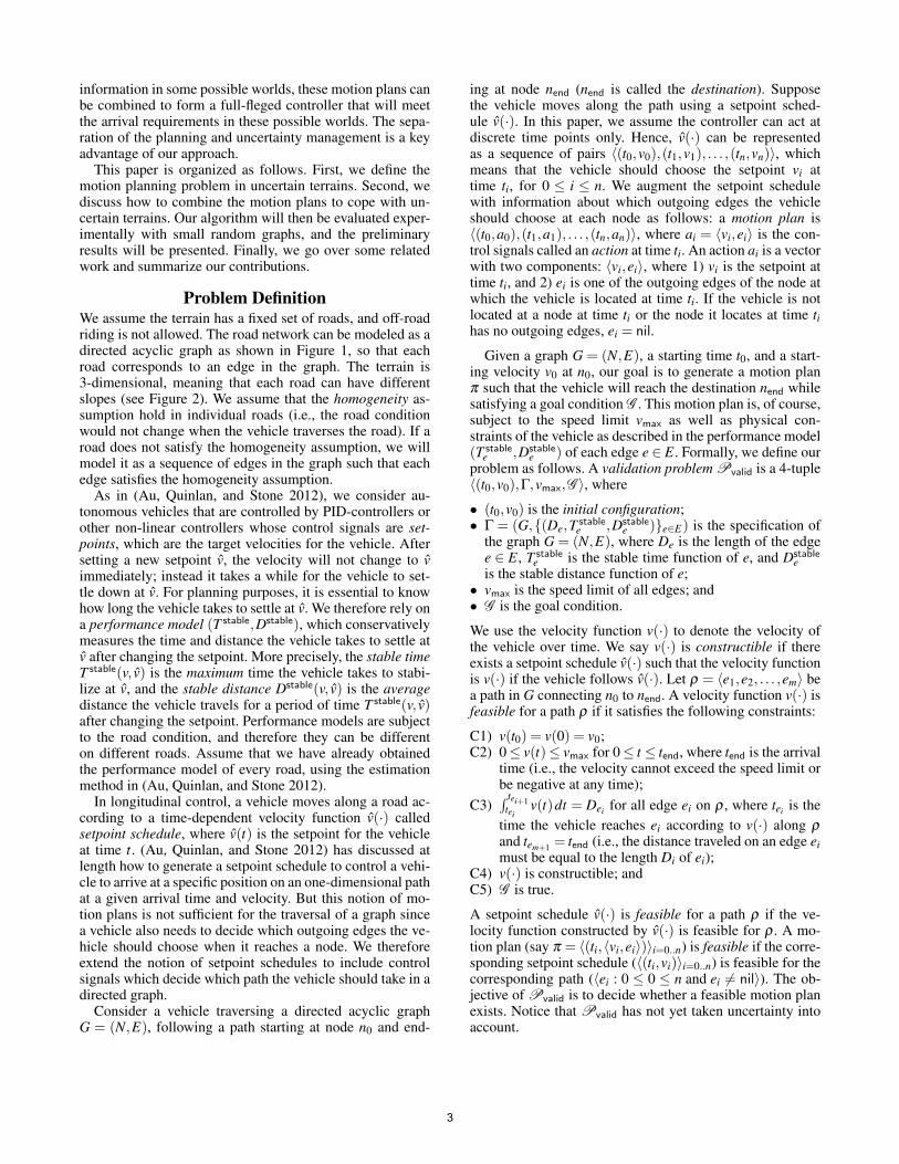
IntroductionOur next frontier of space exploration is near earth objectssuch as Mars and comets. Currently, we rely on robot roversto explore these extraterrestrial lands. However, without fullknowledge of the environment on these lands, it is hard togenerate motion plans for these rovers to achieve their objec-tives. For example, if the vehicle in Figure 1 can only detectthe paths within its sensors’ range (the orange pie shape),how can it arrive at the destination without knowing entiregraph of feasible paths? In this paper, we focus on planningto move a vehicle or a rover to its destination in order to meetcertain requirements at the destination, under the conditionthat the terrain on its way is uncertain.

There have been many works on motion planning underuncertainty in robotics (e.g., (Rekleitis, Meger, and Dudek2006; Nakhaei and Lamiraux 2008; Um et al. 2013)), butfew of them considered complex arrival requirements. Somevariants of the popular probabilistic planning methods suchas probabilistic roadmap (PRM) (Missiuro and Roy 2006;Kneebone and Dearden 2009) and rapidly-exploring ran-dom trees (Melchior and Simmons 2007; Maeda, Singh, and

Copyright c© 2015, Association for the Advancement of ArtificialIntelligence (www.aaai.org). All rights reserved.

Start e1

e2 e3

e4

e5

Destination

Figure 1: A rover traverses an unknown 3D-terrain to reachthe destination. The roads on the terrain are modeled as adirected acyclic graph. The orange pie shape is the sensor’srange.

D1 D2 D3 D4 D5

Start

Initial Condition: Requirements:

Edge e1 Edge e2 Edge e3 Edge e4 Edge e5

Destination

Height

5m

Figure 2: The cross-section of the terrain along the bold pathin Figure 1.

Durrant-Whyte 2011; Nikitenko et al. 2013) can be used togenerate motion plans in uncertain environments. However,their underlying heuristics provide no guarantee of success.While the framework of POMDPs (e.g., (Ong et al. 2010))is rich enough to encode planning problems under uncer-tainty with arbitrary utility functions, some goal conditionscan be too complicated for general-purpose POMDP solversto handle. In fact, without using specialized planners it ishard to satisfy certain goal conditions. We therefore pro-pose a two-stage approach for motion planning under un-certainty: First, use an efficient planner to generate motionplans that meet the arrival requirements in uncertainty-freeenvironments. Second, combine the solution plans generatedby the planner to form a controller that can work in uncertainenvironments. Our approach is inspired by the work on thesynthesis of strategies from interaction traces in (Au, Kraus,and Nau 2008), which outlined the foundation of our ap-proach: by augmenting motion plans with simulated sensing

2

information in some possible worlds, these motion plans canbe combined to form a full-fleged controller that will meetthe arrival requirements in these possible worlds. The sepa-ration of the planning and uncertainty management is a keyadvantage of our approach.

This paper is organized as follows. First, we define themotion planning problem in uncertain terrains. Second, wediscuss how to combine the motion plans to cope with un-certain terrains. Our algorithm will then be evaluated exper-imentally with small random graphs, and the preliminaryresults will be presented. Finally, we go over some relatedwork and summarize our contributions.

Problem DefinitionWe assume the terrain has a fixed set of roads, and off-roadriding is not allowed. The road network can be modeled as adirected acyclic graph as shown in Figure 1, so that eachroad corresponds to an edge in the graph. The terrain is3-dimensional, meaning that each road can have differentslopes (see Figure 2). We assume that the homogeneity as-sumption hold in individual roads (i.e., the road conditionwould not change when the vehicle traverses the road). If aroad does not satisfy the homogeneity assumption, we willmodel it as a sequence of edges in the graph such that eachedge satisfies the homogeneity assumption.

As in (Au, Quinlan, and Stone 2012), we consider au-tonomous vehicles that are controlled by PID-controllers orother non-linear controllers whose control signals are set-points, which are the target velocities for the vehicle. Aftersetting a new setpoint v, the velocity will not change to vimmediately; instead it takes a while for the vehicle to set-tle down at v. For planning purposes, it is essential to knowhow long the vehicle takes to settle at v. We therefore rely ona performance model (T stable,Dstable), which conservativelymeasures the time and distance the vehicle takes to settle atv after changing the setpoint. More precisely, the stable timeT stable(v, v) is the maximum time the vehicle takes to stabi-lize at v, and the stable distance Dstable(v, v) is the averagedistance the vehicle travels for a period of time T stable(v, v)after changing the setpoint. Performance models are subjectto the road condition, and therefore they can be differenton different roads. Assume that we have already obtainedthe performance model of every road, using the estimationmethod in (Au, Quinlan, and Stone 2012).

In longitudinal control, a vehicle moves along a road ac-cording to a time-dependent velocity function v(·) calledsetpoint schedule, where v(t) is the setpoint for the vehicleat time t. (Au, Quinlan, and Stone 2012) has discussed atlength how to generate a setpoint schedule to control a vehi-cle to arrive at a specific position on an one-dimensional pathat a given arrival time and velocity. But this notion of mo-tion plans is not sufficient for the traversal of a graph sincea vehicle also needs to decide which outgoing edges the ve-hicle should choose when it reaches a node. We thereforeextend the notion of setpoint schedules to include controlsignals which decide which path the vehicle should take in adirected graph.

Consider a vehicle traversing a directed acyclic graphG = (N,E), following a path starting at node n0 and end-

ing at node nend (nend is called the destination). Supposethe vehicle moves along the path using a setpoint sched-ule v(·). In this paper, we assume the controller can act atdiscrete time points only. Hence, v(·) can be representedas a sequence of pairs 〈(t0,v0),(t1,v1), . . . ,(tn,vn)〉, whichmeans that the vehicle should choose the setpoint vi attime ti, for 0 ≤ i ≤ n. We augment the setpoint schedulewith information about which outgoing edges the vehicleshould choose at each node as follows: a motion plan is〈(t0,a0),(t1,a1), . . . ,(tn,an)〉, where ai = 〈vi,ei〉 is the con-trol signals called an action at time ti. An action ai is a vectorwith two components: 〈vi,ei〉, where 1) vi is the setpoint attime ti, and 2) ei is one of the outgoing edges of the node atwhich the vehicle is located at time ti. If the vehicle is notlocated at a node at time ti or the node it locates at time tihas no outgoing edges, ei = nil.

Given a graph G = (N,E), a starting time t0, and a start-ing velocity v0 at n0, our goal is to generate a motion planπ such that the vehicle will reach the destination nend whilesatisfying a goal condition G . This motion plan is, of course,subject to the speed limit vmax as well as physical con-straints of the vehicle as described in the performance model(T stable

e ,Dstablee ) of each edge e ∈ E. Formally, we define our

problem as follows. A validation problem Pvalid is a 4-tuple〈(t0,v0),Γ,vmax,G 〉, where

• (t0,v0) is the initial configuration;• Γ = (G,{(De,T stable

e ,Dstablee )}e∈E) is the specification of

the graph G = (N,E), where De is the length of the edgee ∈ E, T stable

e is the stable time function of e, and Dstablee

is the stable distance function of e;• vmax is the speed limit of all edges; and• G is the goal condition.

We use the velocity function v(·) to denote the velocity ofthe vehicle over time. We say v(·) is constructible if thereexists a setpoint schedule v(·) such that the velocity functionis v(·) if the vehicle follows v(·). Let ρ = 〈e1,e2, . . . ,em〉 bea path in G connecting n0 to nend. A velocity function v(·) isfeasible for a path ρ if it satisfies the following constraints:

C1) v(t0) = v(0) = v0;C2) 0≤ v(t)≤ vmax for 0≤ t ≤ tend, where tend is the arrival

time (i.e., the velocity cannot exceed the speed limit orbe negative at any time);

C3)∫ tei+1

teiv(t)dt = Dei for all edge ei on ρ , where tei is the

time the vehicle reaches ei according to v(·) along ρ

and tem+1 = tend (i.e., the distance traveled on an edge eimust be equal to the length Di of ei);

C4) v(·) is constructible; andC5) G is true.

A setpoint schedule v(·) is feasible for a path ρ if the ve-locity function constructed by v(·) is feasible for ρ . A mo-tion plan (say π = 〈(ti,〈vi,ei〉)〉i=0..n) is feasible if the corre-sponding setpoint schedule (〈(ti,vi)〉i=0..n) is feasible for thecorresponding path (〈ei : 0 ≤ 0 ≤ n and ei 6= nil〉). The ob-jective of Pvalid is to decide whether a feasible motion planexists. Notice that Pvalid has not yet taken uncertainty intoaccount.

3

Motion Planning in Uncertain TerrainsThis section concerns with situations in which the terrain isnot fully observable. At the beginning, the vehicle knowsnothing about the terrain beyond the range of its sensors, ex-cept the location of the destination nend. Suppose the vehiclestarts with a belief about the set G of possible graphs. Thebelief is defined in terms of a probability distribution P overG, which means that the probability that a possible graphG ∈ G is the real graph is P(G). As the vehicle traversesthe graph, it gathers more and more information about theterrain over time. This information will be helpful for thevehicle to ascertain which graph in G is real.

Let G = {G1,G2, . . . ,GmG} where Gi = (Ni,Ei) for 1 ≤i≤mG. Some of the nodes and edges are shared by multiplegraphs in G. Let Ns =

⋃1≤i≤mG

{Ni} and Es =⋃

1≤i≤mG{Ei}.

The union of all graphs in G forms a supergraph Gs =(Ns,Es). Consider the 2D rectangular region R that physi-cally contains Gs. We subdivide the region into a lx× ly gridas shown in Figure 1. Each cell in the grid will generate asignal when the sensors on the vehicle gather informationabout the cell. The signal of a cell reflects some features ofthe terrain at the cell (e.g., landmarks). From the sensors’viewpoint, a terrain is a mapping T : [1 . . . lx]× [1 . . . ly]→ S,which specifies the signals at all cells in R, where S is theset of all possible signals. Each possible graph Gi ∈G is as-sociated with a terrain Ti. Suppose the real graph is Gi. Atthe beginning, the vehicle has only partial knowledge of Ti.The vehicle will use its sensors to gather more informationabout Ti during traversal. We will make use of the mono-tonicity assumption: Any new knowledge from sensors willnot contradict the existing ones.

Suppose the vehicle follows a feasible motion plan π =〈(t0,a0),(t1,a1), . . . ,(tn,an)〉, where ai = 〈vi,ei〉. We assumesensing actions interleave with the execution of actions: Be-fore the execution of an action ai at time ti, the vehicle ob-tains a percept bi from the environment. We define an aug-mented motion plan as τ = 〈(a1,b1),(a2,b2), . . .(ak,bk)〉,which is basically an interaction trace between the vehicleand the environment. Now we make use of the results in (Au,Kraus, and Nau 2008), which states that a set of interactiontraces, under certain conditions, can be combined to forman agent that will succeed in environments in which the in-teraction traces are generated. Furthermore, if we carefullyselect the interaction traces, we can increase the probabil-ity that the agent will succeed in an uncertain environment.Algorithm 1 is the architecture of the vehicle’s controllerthat makes use of augmented motion plans. In Algorithm 1.actioni(τ) and percepti(τ) be the i’th action and the i’th per-cept of τ , respectively.

According to (Au, Kraus, and Nau 2008), the interactiontraces can be combined to form a composite agent if they aremutually compatible. In the same vein, we define the com-patibility of augmented motion plans as follows.Definition 1 Let lcp(αa,αb) be the longest common pre-fix of two finite sequences αa = 〈ca

1,ca2, . . . ,c

aka〉 and αb =

〈cb1,c

b2, . . . ,c

bkb〉, such that lcp(αa,αb) = 〈c1,c2, . . .ck〉 where

ci = cai = cb

i for 1 ≤ i ≤ k and either (1) k = ka < kb, (2)

Algorithm 1 The architecture of the vehicle’s controller.1: procedure VEHICLECONTROLLER(T )2: i := 1; Ti := T3: while the vehicle has not reached nend do4: if the current time is ti then5: Obtain a percept bi from sensors.6: Ti+1 := /07: for all τ ∈Ti do8: if bi = percepti(τ) then9: Ti+1 := Ti+1∪{τ}

10: Ai := {actioni(τ) : ∀τ ∈Ti+1}11: if |Ai| 6= 1 then12: Return Fail since T is not compatible.13: Let the unique action in Ai be 〈vi,ei〉14: if ei 6= nil then steer the vehicle to edge ei.15: Change the current setpoint to vi16: i := i+1

k = kb < ka, or (3) cak+1 6= cb

k+1.

Definition 2 Two augmented motion plans τ1 and τ2 arecompatible if and only if |lcp(action(τ1),action(τ2))| >|lcp(percept(τ1),percept(τ2))|, where action(〈(ai,bi)〉i..k)= 〈ai〉i=1..ka and percept(〈(ai,bi)〉i..k) = 〈bi〉i=1..kb .

Definition 3 A set T of augmented motion plans is compa-tiable if and only if every pair of augmented motion plans inT is compatiable.

Theorem 1 states that if the input T of Algorithm 1 is com-patible, the algorithm will never return Fail from Line 12.The proof of the theorem is similar to the proof in Theo-rem 2 in (Au, Kraus, and Nau 2008).

Theorem 1 Algorithm 1 will not fail if 1) T is compatible,and 2) one of the augmented motion plans in T is generatedby the real graph.

Theorem 1 implies that if we can find a compatible setT of feasible augmented motion plans, Algorithm 1 willalways be able to reach its destination while satisfying thegoal condition, as long as the real graph is one of the graphsin which some feasible augmented motion plans in T aregenerated. Of course, we assume that the underlying plannerfor the validation problem can generate motion plans thatsatisfy the goal condition. For instance, if we concern witharriving at the destination at a specific time and at a specificvelocity, the algorithms presented in (Au, Kraus, and Nau2008) will work.

The probability of success of Algorithm 1 is equal to∑τi∈T {P(Gi)}, where τi is a feasible augmented motionplan generated in Gi. As can be seen, if T includes oneaugmented motion plan in every G ∈ G, the probability ofsuccess is 1—the vehicle can guarantee to arrive at the desti-nation in uncertain terrains. However, not every pair of aug-mented motion plans is compatible. In fact, there can be twopossible graphs whose sets of all feasible augmented mo-tion plans are disjoint, meaning that it is impossible to havea 100% successful rate. In these uncertain terrains, we canonly hope to maximize the probability of success by finding

4

Algorithm 2 The greedy selection of compatible augmentedmotion plans.

1: procedure FINDCOMPATIABLEPLANS(G)2: T := /03: for Gi ∈G in descending order of P(Gi) do4: for j = 1 to K do5: Randomly generate a motion plan π in Gi6: Simulate percepts as vehicle follows π in Gi7: Let τ be the augmented motion plan of π .8: if τ is compatible with all τ ′ ∈T then9: T := T ∪{τ}; Break

return T

a large T that covers as many possible graphs as possible.Hence, we present a greedy algorithm to find such T . Thealgorithm, as shown in Algorithm 2, considers the possiblegraph in the descending order of probability, and then ran-domly generates K augmented motion plans in these graphs.The augmented motion plan will be added to T as long asit is compatible with all plans in T . Although the algorithmcannot guarantee to find T that maximizes the probabilityof success, it can often find a good set of augmented mo-tion plans with a high probability of success, as shown inthe experimental results in the next section.

Preliminary Experimental ResultsTo evaluate Algorithm 1 and Algorithm 2, we conducted asimulation experiment with four different random graphs.One of the random graphs is shown in Figure 3. First, a di-rected acyclic graph Gs that connects n0 to nend was gen-erated by randomly connecting a fixed number of nodes(Graph a). Gs has to be solvable (i.e, there exist paths con-necting n0 to nend). Second, we randomly chose the roadcondition T stable and Dstable for each edge, and assignedlandmarks to each of the edges, such that the landmarks ontwo different edges are different. Third, we randomly re-moved some edges in Gs to form graphs (Graph b-e). Thelandmarks on the removed edges were removed too. We re-peated the removal of edges from Gs four times to generatea set G of four possible graphs.

After generating G, we set the starting time t0 = 0s andthe starting velocity v0 = 0m/s. Our goal G is to reach nend

at time tend = 100s and vend = 40m/s. We devised a motionplanning algorithm to generate one augmented motion planfor each possible graph. Then we randomly assigned a prob-ability distribution P over G, and ran Algorithm 2 to find aset T ′ of compatible augmented motion plans. We ran Algo-rithm 1 with T ′ 100 times and measured the probability ofsuccess. We repeated the measurement 6 times with differ-ent probability distributions. The successful rates and their95% confidence intervals are shown in Table 1.

As can be seen, the success rate of our approach is oftenhigher than 90%, with an overall successful rate of 97.4%While different probability distributions of G produce sim-ilar successful rates, the successful rates heavily depend onthe topology of the original supergraph Gs. In Gs

2, the suc-

A B

C E

D F

G H

START END

A B

C

D F

G H

START END

A B

E

F

G H

START END

A B

C E

D F

G H

START END

A B

C

D F

G H

START END

(a)

(b) (c)

(d) (e)

Figure 3: Graph a is Gs, and Graph b-e are the possiblegraphs.

Table 1: The successful rates of Algorithm 2.Graph Gs

1

Prob. Distribution Success Rate(0.5,0.2,0.1,0.2) 94.1%±5.2(0.4,0.3,0.2,0.1) 95.1%±3.1(0.2,0.1,0.3,0.4) 93.2%±3.6(0.1,0.5,0.2,0.2) 90.0%±3.7(0.2,0.1,0.4,0.3) 90.3%±2.8(0.3,0.3,0.1,0.3) 89.6%±2.2

Graph Gs2

Prob. Distribution Success Rate(0.5,0.2,0.1,0.2) 100%±0(0.4,0.3,0.2,0.1) 100%±0(0.2,0.1,0.3,0.4) 100%±0(0.1,0.5,0.2,0.2) 100%±0(0.2,0.1,0.4,0.3) 100%±0(0.3,0.3,0.1,0.3) 100%±0

Graph Gs3

Prob. Distribution Success Rate(0.5,0.2,0.1,0.2) 98.6%±2.3(0.4,0.3,0.2,0.1) 99.1%±1.3(0.2,0.1,0.3,0.4) 99.4%±0.8(0.1,0.5,0.2,0.2) 99.5%±0.7(0.2,0.1,0.4,0.3) 99.3%±0.7(0.3,0.3,0.1,0.3) 98.3%±1.0

Graph Gs4

Prob. Distribution Success Rate(0.5,0.2,0.1,0.2) 100.0%±0.0(0.4,0.3,0.2,0.1) 99.1%±0.4(0.2,0.1,0.3,0.4) 99.5%±0.7(0.1,0.5,0.2,0.2) 99.5%±0.6(0.2,0.1,0.4,0.3) 99.8%±0.4(0.3,0.3,0.1,0.3) 99.0%±0.5

cessful rates are 100%, meaning that the augmented motionplans of the possible graphs are highly compatible.

Related WorkProbabilistic roadmap methods (PRM) (Kavaki et al. 1996)and rapidly-exploring random trees (LaValle and JamesJ. Kuffner 2000) are both widely used, sampling-based al-gorithms. These algorithms are incomplete, but some exten-sions have been made to turn them into complete algorithms.Hirsch and Halperin (2004) and Zhang et al. (2007) pro-posed a hybrid motion planner that generates complete so-lutions with PRM. Nonetheless, these modified algorithmswill suffer from inefficiency due to their completeness, andthe arrival requirement has to be quite simple (e.g., arrive ata position without time and velocity requirement). While in-terleaving planning and execution is a good strategy to dealwith uncertainty in planning (e.g., (Pivtoraiko, Mellinger,and Kumar 2013)), replanning cannot correct wrong deci-sions in previous steps, thus it is hard to provide any arrivalguarantees.

TPOPEXEC (Muise, Beck, and McIlraith 2013) intro-duces a two-stage approach for planning: First, an offlinepreprocessor takes a partial-order plan and a set of temporal

5

constraints to produce a generalized representation. Second,an online component called EXECUTOR selects a tempo-rally consistent, valid plan fragment from the generalizedplan. Choset et al. (2000) presented a sensor-based motionplanning approach based on a roadmap called hierarchicalgeneralized Voronoi graph (HGVG), which can be incre-mentally constructed using only line-of-sight sensor data.This approach guarantees that the robot can find a path fromstart to goal or report that such a path is not feasible. Lunaet al. (2014) introduces a two-stage framework for efficientcomputation of an optimal control policy in the presence ofuncertainty. It first generates a bounded-parameter Markovdecision process (BMDP) over a discretization of the en-vironment and then quickly selects a local policy withineach region to optimize a continuously valued reward func-tion online. As the sensors gather more information aboutthe environment, the BMDP is updated accordingly and theglobal control policy is recomputed. However, none of theabove approaches concern with arrival requirements otherthan reaching the destination.

Concluding RemarksIn this paper, we proposed a two-stage approach for mo-tion planning in uncertain terrains. More specifically, weproposed to augment motion plans with sensing informa-tion and then combine them, in a greedy manner, to forma controller that can handle uncertainty in the environment.This separation of planning and uncertainty managementcan greatly simplify our task, as we can utilize existing fastplanners to generate motion plans that satisfy the goal condi-tions. In space exploration applications, the goal conditionscan be quite specific. Instead of modifying existing plan-ning algorithms for these applications to deal with uncer-tain terrains, we propose to adopt them directly and combinetheir solutions to form a contingency controller. If there areenough augmented motion plans, the controller can achievea high success rate.

Our approach has two drawbacks. First, the number ofcontingencies can be quite large in an uncertain environ-ment, meaning that we may need a lot of augmented mo-tion plans in order to deal with all these contingencies. How-ever, we believe that in some environments, a small numberof augmented motion plans is sufficient because one aug-mented motion plan can deal with several different contin-gencies in different possible graphs. We intend to evaluatethis possibility in the future. Second, we usually do not knowthe set of all possible graphs in G ahead of time, thus somepossible graphs are not considered by Algorithm 2. As dis-cussed in (Au, Kraus, and Nau 2008), we can use a backupplanner to handle these unknown cases. In the future, we in-tend to improve our algorithms to address these issues.

ReferencesAu, T.-C.; Kraus, S.; and Nau, D. 2008. Synthesis of strate-gies from interaction traces. In Proceedings of the Inter-national Joint Conferenceon Autonomous Agents and MultiAgent Systems (AAMAS), 855–862.

Au, T.-C.; Quinlan, M.; and Stone, P. 2012. Set-point scheduling for autonomous vehicle controllers. InIEEE International Conference on Robotics and Automation(ICRA), 2055–2060.Choset, H., and Burdick, J. 2000. Sensor-based exploration:The hierarchical generalized voronoi graph. The Interna-tional Journal of Robotics Research 19(2):96–125.Hirsch, S., and Halperin, D. 2004. Hybrid motion planning:Coordinating two discs moving among polygonal obstaclesin the plane. In Algorithmic Foundations of Robotics V. 239–255.Kavaki, L. E.; Svestka, P.; Latombe, J.-C.; and Overmars,M. H. 1996. Probabilistic roadmaps for path planning inhigh-dimensional configuration spaces. IEEE Transactionson Robotics and Automation 12(4).Kneebone, M., and Dearden, R. 2009. Navigation plan-ning in probabilistic roadmaps with uncertainty. In Interna-tional Conference on Automated Planning and Scheduling(ICAPS), 209–216.LaValle, S. M., and James J. Kuffner, J. 2000. Rapidly-exploring random trees: progress and prospects. In Algorith-mic and Computational Robotics: New Directions, 293–308.Luna, R.; Lahijanian, M.; Moll, M.; and Kavraki, L. E.2014. Optimal and efficient stochastic motion planning inpartially-known environments. In AAAI Conf. on ArtificialIntelligence.Maeda, G. J.; Singh, S. P. N.; and Durrant-Whyte, H. 2011.A tuned approach to feedback motion planning with RRTsunder model uncertainty. In ICRA, 2288–2294.Melchior, N., and Simmons, R. 2007. Particle rrt for pathplanning with uncertainty. In ICRA, 1617–1624.Missiuro, P. E., and Roy, N. 2006. Adapting probabilisticroadmaps to handle uncertain maps. In ICRA, 1261–1267.Muise, C.; Beck, J. C.; and McIlraith, S. A. 2013. Flexibleexecution of partial order plans with temporal constraints. InProceedings of the Twenty-Third international joint confer-ence on Artificial Intelligence, 2328–2335. AAAI Press.Nakhaei, A., and Lamiraux, F. 2008. A framework for plan-ning motions in stochastic maps. In Proceeding of Inter-national Conference on Control, Automation, Robotics andVision.Nikitenko, A.; Riga, L.; Ekmanis, M.; and Liekna, A. 2013.Rrts postprocessing for uncertain environments. In Proceed-ings of International Conference on Systems, Control andInformatics, 171–179.Ong, S. C. W.; Png, S. W.; Hsu, D.; and Lee, W. S. 2010.Planning under uncertainty for robotic tasks with mixedobservability. International Journal of Robotics Research29(8):1053–1068.Pivtoraiko, M.; Mellinger, D.; and Kumar, V. 2013. In-cremental micro-uav motion replanning for exploring un-known environments. In IEEE International Conference onRobotics and Automation (ICRA), 2452–2458.Rekleitis, I.; Meger, D.; and Dudek, G. 2006. Simultaneousplanning, localization, and mapping in a camera sensor net-work. Robotics and Autonomous Systems 54(11):921–932.

6

Um, D.; Gutierrez, M. A.; Bustos, P.; and Kang, S. 2013.Simultaneous planning and mapping (spam) for a manipula-tor by best next move in unknown environments. In IROS,5273–5278.Zhang, L.; Kim, Y. J.; and Manocha, D. 2007. A hybridapproach for complete motion planning. In IEEE/RSJ Inter-national conference on Intelligent Robots and Systems.

7