proceedings of the ieee, vol. 70, no. 3, march...

PROCEEDINGS OF THE IEEE, VOL. 70, NO. 3, MARCH 1982 229

Multiplied-Poisson Noise in Pulse, Particle, and Photon Detection

I. INTRODUCTION ENTION THE TERM point process and the electrical engineer is likely to imagine highly localized events of a particular kind occuning along a time axis: the emis-

sion of electrons from a cathode or perhaps the registration of nuclear particles in a detector. But such processes form an intimate part of our daily lives as well. Few of us think of walking along the sidewalk or driving down the road in mathematical terms, yet to the operations researcher studying traffic flow, these acts are representable in terms of important point processes. Every field of scientific endeavor boasts its own examples.

Probably the simplest and most widely occurring point process is the one-dimensional homogeneous Poisson process [ 11 4 3 1 . It plays the role that the Gaussian process does in the theory of

This work was supported by the Joint Services Electronica Program Manuscript received February 3, 1981; revised January 11, 1982.

(US. Army, U.S. Navy, and US. Air Force) under Contract DAAG29- 79-C-0079, and the National Science Foundation under Grant ENG78- 26498.

B.E.A. Saleh b with the Department of Electrical and Computer

the Columbia Radiation Laboratory. Department of Electrical Edgi- Engineering, University of W s c o ~ i n , Madison, WI 53706, and with

neering, Columbia University, New York, NY 10027. M. C. Teich is with the Columbia Radiation Laboratory, Department

of Electrical Engineering, Columbia University, New York, NY 10027.

continuous stochastic processes. The homogeneous Poisson point process (HPP) is characterized by a single quantity, its rate, which is constant. One of its distinguishing features is that it evolves in time without aftereffects. This means that the occurrence times and number of events before an arbitrary time have no bearing on the subsequent occurrence times and number of events. It is said to have zero memory.

Because of its simple properties, the HPP turns out to be a suitable building block for more complex point processes that appear to resemble the Poisson process little, if at all. We all recall, no doubt, a very important property of this process: pass an HPP through a lined filter and out comes shot noise. This result is probably just a shade younger than electrical engineering itself.

There are many generalizations of the H€T. One case that has been studied extensively is the doubly stochastic Poisson point process (DSPP), which diffels from the HPP in that the rate is no longer constant. Rather, it takes on a stochastic nature of its own. This process was f i t examined by Cox (and by Bartlett in the discussion to Cox’s paper) [41. Cox provided an example of its use in textile technology. The designation DSPP w a ~ introduced to emphasize that two kinds of randomness occur: randomness associated with the Poisson point process itself and an independent randomness associated with its rate. The earliest connection of the DSPP with electrical engineering appears to be in the work of Darling and Siegert [SI and Siegert [61. The DSPP subsequently became the basis for understanding the photodetection of light, and many of the early papers in this area [7] -[ 151 drew heavily on results derived in connection with classical radio receiver communications and noise [ 161 -[ 181. At the same time, the DSPP arose in the context of the detection of acoustic noise in the auditory system [ 19 I . , A number of excellent secondary sources, detailing the history and properties of the DSPP, are available [3] , [201-[271.

In certain areas of study, multiplication effects in point processes play an important role; in most such cases, a given (primary) point process is multiplied in some fashion to give rise to a second (subsidiary) point process. Cathodolumines- cence 128 I , [ 29 I , which is responsible for the television, oscilloscope, and radar images, provides a simple but i m p o p t example. Each eiectron incident on the phosphor in the screen releases a random number of photons, which form the image that we observe. Multiplication can also occur in successive stages, so that each generation of particles produces a new generation, and so on. Such branching (cascade) processes can be used to describe the noise properties of devices like avalanche detectors and electron multipliers [ 301 , [ 3 1 ] .

There have been many theoretical characterizations of the multiplication of events. In the mathematical-statistics com-

0018-9219/82/0300-0229500.7~ 0 1982 IEEE

230

munity, the formulations have been complete but often too general [321 to be directly useful in electrical engineering. In the electron-device noise community, on the other hand, effective formulations have been developed, but they have been framed almost exclusively in terms of the lowest-order properties of these processes: the mean, variance, and spectrum [ 3 1 1 , [ 331 ; the multiplication, furthermore, has been assumed to be instantaneous in most of these treatments. Additional information about the physical nature of a process can be gleaned from its higherarder properties. Measurements of the probability density of the time between consecutive events, for example, or the number of events registered in a fixed counting time, can provide valuable clues about underlying physical mechanisms.

Indeed, subsidiary events are often not generated instantaneously, and the multiplication properties alone are insuf- ficient to characterize such a process. In many physical situations, there will be delay relative to the primary event in accordance with a particular probability law, so that the time behavior of the multiplication process comes into play.

In this paper, we examine the. properties of a particular multiplication model that incorporates time effects, and is both mathematically tractable and useful in electrical engineering and physics. The subsidiary process is taken to be a Poisson point. process whose rate is a linearly filtered version of the primary process, which is assumed to be an HPP. Since an HPP passed through a linear fiter yields shot noise, we call our process a shot-noisedriven doubly stochastic Poisson point process (SNDP). It is a special case of the DSPP. Each primary event is multiplied into subsidiary events, but with a time course prescribed by the linear fiiter impulse response function. Thus event multiplication and dynamics are combined into one model. Bartlett [34] proposed a similar twodimensional model for use in plant ecology some time ago, whereas Vere- Jones and Davies constructed this kind of formulation (they called it a “trigger” model) in connection with the study of earthquake occurrences [ 35 I . Bartlett explicitly showed that the SNDP is a special but important example of a cluster point process developed by Neyman and Scott [36], [37] to describe the distribution of galaxies in space. This identity is explored by Lawrance in his excellent contribution to the point-process book edited by Lewis [ 21 1.

In Section 11, we describe random events arising from multiplication processes. The properties of the SNDP, including the counting statistics and time statistics, are provided in Sec- tion 111. In Section IV, we treat the multifold statistics and spectrum. A number of important applications of the SNDP are considered in Section V, including scintillation detection, photomultiplier noise induced by ionizing radiation, cathodoluminescent emission, electronography, and X-ray radiography. The conclusion is provided in Section VI.

n. RANDOM EVENTS ARISING FROM MULTIPLICATION PROCESSEs

A. Instantaneous Multiplication Consider the primary point process whose events are illus-

trated in Fig. l(a). The number of events (counts) within a time interval [0, TI is a discrete random variable m having a moment-generating function (mgf), e,($) = (exp (-sm)). The angular brackets represent an ensemble average. Let each primary event produce independently A subsidiary events (as illustrated in Fig. l(b)), where A is a discrete random variable that has an mgf QA(s) = (exp (-SA)). The total number of

PROCEEDINGS OF THE IEEE, VOL. 70, NO. 3, MARCH 1982

i

0

Fig. 1. Random multiplication of events. (a) Primary events. (b) Sub- sidiary events. (c) Randomly delayed subsidiary events.

secondary events n is given by

n = x A k k = 1

where A& are independent values of A . If A and m are statistically independent, then it can be shown [ 1 1, [ 3 11, [ 331 that the rngf of n, Q,(s) = (exp ( - s n ) ) , is given by

Q n b ) = Qm(-ln QA(s)). (1)

This equation can be used to relate the moments of n to those of m and A. The means are related by

( n ) = ( A ) (m), (2)

the second factorial moment obeys the equation

(n (n - 1)) = (A)2(m(m - 1)) + (m) U(A - l)), (3)

and the variances are expressed as var ( n ) = ( A > ~ var (m) + (m) var (A). (4)

Equation (4) is known as the Burgess variance theorem [38], (391.

When the primary events constitute a Poisson point process, the random variable m has a Poisson distribution with mgf

Q,(s) = exp [(m) ( e -S - 1) l ( 5 )

which, when combined with ( l ) , gives rise to

QAs) = exp [(m) ( Q A ~ ) - 111. (6)

The count variance associated with (6) is then

var ( n ) = (1 + a l ) (n ) , (7)

where

a1 =- var(A) +(A)- 1. (A)

Equation (7) demonstrates that for a Poisson primary process, whatever the distribution of the multiplication factor A , the variance of n is always proportional to the mean (n). The ratio var (n)/ (n> is known as the dispersion ratio or the Fano factor [31]. We denote parameter a l as the excess Fano factor.

SALEH AND TEICH: MULTIPLIED-POISSON NOISE 231

When the multiplication factor A also has a Poisson distribution, ( 6 ) yields

Q,(s) = exp (%{ exp [ ( A ) (e-’ - 1)l - 1 , (9) 1) which is the mgf for the Neyman Type-A distribution [401, [41], [2], [19], [26], [371. The variance is obtained from (7) and (8) :

a1 =(A). (10)

The Neyman Type-A distribution has a variance larger than that of a Poisson distribution of the same mean.

When the random variable A is describable instead by a Bernoulli distribution, which associates the values 1 and 0 with the probabilities (A) and (1 - (A)), respectively, the factor a1 equals 0 and n is Poisson. The Poisson distribution is therefore invariant against Bernoulli random multiplication or deletion [ 1 1 . It should also be noted [ 241 that all DSPP’s are invariant under Bernoulli Selection (in the sense that the random integrated rate W is reduced to ( A ) W , see Appendix A). WhenA has a geometric (Bose-Einstein) distribution, a1 = 2 (A) ; this is sometimes called the Polya-Aeppli distribution. Values of a1 for other distributions can be easily obtained [2], [3 1 1 , [33].

B. Multiplication with Random Dehy In the previous subsection (Fig . l(a), (b)), a primary event

was assumed to instantaneously excite a random number of subsidiary events. In many physical systems, a time delay will be inherent in the multiplication process, and that time delay will itself be random, as illustrated in Fig. l(c). The primary events may or may not be included in the final point process.

The nature of the randomness of the delay times that sepa- rate subsidiary events from their primary event can take different forms. In the Neyman-Scott model [361, (371, the primary process is taken to be an HPP, which is excluded from the final process. The multiplication factor can assume an arbitrary distribution, and the delay times, ~ 1 , 7 2 , * * * , TA , measured from the primary event, are assumed to be statistically independent and identically distributed. This process has been used by Neyman and Scott to describe a broad variety of phenomena from the distribution of larvae on small plots of land to the distribution of galaxies in space. It has also been used by Vere-Jones [42], in connection with the occurrences of earthquakes in New Zealand. In the Bartlett-Lewis model 1431, 1441, primary events are again described by an HPP, but they are included in the final point process. Again, the multiplication factor has arbitrary statistics. In this case, time intervals between successive subsidiary pulses that belong to a common primary event, AT^, A72, - * - , A ~ A , are assumed statistically independent and identically distributed, Le., they form a segment of a renewal process. This process has been used by Bartlett [43] for traffic studies and by Lewis [ 4 4 1 for the distribution of computer failure times.

C. The Shot-Noise-Driven Doubly Stochastic Poisson Point Process

We characterize the randomness of both the multiplication factor and the delay times by assuming that an inhomogeneous Poisson process produces the secondary events. The occurrence of a primary event (at t = 0 , for example) is considered to. generate a continuous (usually decaying) function h(r) which acts as the rate of the inhomogeneous Poisson process.

Fig. 2. Production of SNDP events. (a) primary Poisson events. (b) Filtered Poisson wents (shot noise). (c) Subsidiary doubly stochastic Poisson events whose rate is shot noise.

Fig. 3. Model for generrrtion of the SNDP.

The multiplication factor has a Poisson distribution of mean

a

(A) = h(t) dr. (11)

The delay times 71,72, - * - ,7,g are statistically independent and identically distributed with a probability density function [11-[31, [271

P ( 7 ) = h(7) exp [ -6’ h ( t ) d t ] / [ 1 - e - rh( f )a t ] . (12)

This process is therefore a special case of the Neyman-Scott model-a case in which A is Poisson with a mean given by (1 l), and with a delay-time distribution given by (12). The interevent times are not identically distributed because of the non- stationarity of the rate; therefore, this process is not a special case of the Bartlett-Lewis model.

It will be useful to consider matters from an alternative point of view. The sum of the functions associated with primary events that occur at the times ( t i )

X(t) = h(t - ti) i

constitutes a filtered Poisson process, or shot noise (as illustrated in Fig. 2). If the primary events are stationary, this will also be a stationary stochastic process The subsidiary events now form a DSPP whose stochastic rate is the shot noise X(t); this provides the rationale for the name SNDP. The structure of the model is schematically illustrated in the block diagram of Fig. 3, which shows its multiplicative Poisson nature. Physical systems that are describable by an SNDP model will exhibit a physical structure characterized by these three cascaded blocks. Several examples are presented in Section V.

In. PROPERTIES OF THE SHOT-NOISE-DRIVEN DOUBLY STOCHASTIC POISON POINT PROCESS

A block diagram for the SNDP is presented in Fig. 3. A homogeneous Poisson point process of rate p is filtered by a

232 PROCEEDINGS OF THE IEEE, VOL. 70, NO. 3, MARCH 1982

time-invariant linear filter, with a nonnegative impulse response function h(t), resulting in a shot noise process h(t). The process h(t) forms the stochastic rate for a DSPP,f ( t ) . An important parameter is the average number of secondary events produced per primary event 01). For simplicity we shall use the symbol a = (A) , so that (see (1 1))

00

a= 1 h(f) dt . (14)

The process is completely described by the parameter p and the function h(f). We assume, also for simplicity, that t is the only important variable in the stochastic process h. In certain applications, e.g., photocounting detection, spatial variables may also play a role, and this can be incorporated into the model without difficulty. We are interested in determining the statistical properties of the SNDP, including 1) counting statistics, i.e., the statistics (probability distribution and moments) of the number n of events (counts) registered in the time interval [0, TI ; 2) time statistics, i.e., the probability density functions for the forward recurrence time and the interevent time; and 3) multifold statistics, including the joint probability distribution of the numbers of counts n l , n2 , * * in multiple adjacent time intervals, and their moments. This task can be achieved by a straightforward application of the statistical properties of a general DSPP [3], [4], [24], [26], [27], and of shot noise [ 11, [ 161, [451-[471. These properties are reviewed in Appendexes A and B, respectively. In this section we discuss the singlefold statistics; in Section IV, the multifold statistics are presented.

As indicated in Appendix A, it is useful to define the random variable

W = lT h( f ) d t , (15)

which represents the integrated rate of events of the process over the interval [0, TI . Once the moment-generating function of W, Qw(s) = (exp (-sW)), is determined, the singlefold statistics of a DSPP can be directly determined by use of the simple formulas presented in Appendix A. These include the mgf &(s) for the number of counts n, the probability distribution p ( n ) , and the factorial moments Fim). Also included are the probability density functions P ~ ( T ) and P ~ ( T ) for the forward recurrence time (time from an arbitrary point to the first event) and for the interevent time, respectively.

To determine the mgf of the integrated rate W, we require knowledge of the statistics of the rate h(t). In our case, fortu- nately, X(t) is a shot-noise process whose properties are well- known (see Appendix B). In particular the momentgenerating function is

00

Q ~ ( s ) = ( e - ~ ) = e x p { p 11 d t } . (16)

The random variable W is the integral of a shot noise process h(t) over an interval [ O , T I . We note that the integral of a shot noise is simply another shot noise. Thus we can regard W as a sample of a shot-noise process, generated by a homogeneous Poisson point process of rate p, and filtered by a linear filter of impulse response hT(t), which is simply a convolution of h ( t ) with an integrator over the time interval [0, TI. This

LINEAR FILTER h-, [ I 1

Fig. 4. Model for generation of the integrated rate W.

is shown schematically in Fig. 4, whence

hT(t) = dT h(t + t ' ) dt' . (1 7)

Thus the mgf for W becomes

Qw(s)= exp [e { 1: -s* T 0 ) - 1 ] d t }. (18)

An alternative route to deriving (1 7) and ( 18) is to write W = h(iAt)At and use the multifold mgf for (h ( f i ) } , presented

in (B9), in the limit (s i } = s. Given the mgf of W, represented in (18), we now proceed to

determine the statistics of n, as a function of p, T, and h(t) by using (A4) and (A5), and the probability density functions for the forward recurrence time and the interevent time, by using (A71449).

A . Counting Statistics for the SNDP The SNDP is a special DSPP whose integrated rate W is de-

scribed by the momentgenerating function given in (18). In this section we use (A4)-(A6) to determine the statistics (moments and probability distribution) for the number of counts n registered in the time interval [ O , TI . We consider several limiting and special cases.

1 ) The Moments of n: Using (1 8) and (A4) we have derived the following recurrence relation for the mth-order factorial moment of n :

where the coefficients al are . I--

and the mean number of counts (n) is OD 00

(n ) = p j- hT(t) d t = pT h(f) d f = p a r

The first four factorial moments are explicitly written as


An important property of any DSPP, and therefore of the SNDP in particular, is that it is over-dispersed relative to the HPP. This means that the count variance, var ( n ) , is greater than that for an HPP of the same mean, as is evident from (22).

An equally important property of the SNDP is the fact that the variance is proportional to the mean. This is the property discussed previously, in connection with a Poission primary process and instantaneous multiplication with arbitrary statistics (see (7)). The parameter al (the excess Fano factor) is, for the SNDP,

a1 = alf 9 (23)

where

with

[(TI = JW h( t )h( t + r ) d t / [ J m h ( t ) dtj’. (25)

The excess Fano factor, which determines the excess multiplication noise, is therefore directly proportional to the multiplication parameter a (the average number of secondary events per primary event), and inversely proportional to the parameter f ,which we refer to as the number of degrees of freedom. It will be shown subsequently that in the limit of long counting times, i.e., T >> r p , where rp is the characteristic time scale of h ( t ) , R approaches 1. In the opposite limit, i.e., T << r p , f approaches r p / T , a large number.

Another parameter of interest is the coefficient of skewness, S, which is given by

S=(An3)/[(AnZ)I3/’ =(n)-’I2 ( 1 + 3 ~ ~ + a ~ ) / ( l + a ~ ) ~ / ~ . (26)

For an HPP, S = (n)- lI2. 2 ) The Probability Dism‘bution of n: Using (AS), together

with (1 8), we obtain the following recurrence relation for the counting distribution p ( n ) :

--OD

n

I=O ( n + l ) p ( n + 1) = (n) 2 Clp(n - 2 )

where the coefficients CI are determined by the shape of the impulse response function h T ( t ) through

Equations (27) and (28) are derived by forming the nth deriva- tive of both sides of (18), applying the Leibnitz rule, and using (A5).

3) Counting Statistics in the Limit of Long Counting Time: When the counting time T is much longer than the characteristic time scale of the impulse response function h( t ) , we can

replace ( 17) by the approximation

t a, - T < t < O

0, elsewhere. h d t ) =

Consequently, ( 18) yields

where ( n ) = p T . Examination of (29) shows that W has a fiied-multiplicative Poisson distribution, i.e., it takes on the values 0, a, 2a, - * , ka, * * where k has a Poisson distribution [48]. This is, of course, to be expected because of the assumption that h ( t ) is very narrow. Using (A2) we obtain

which is precisely the mgf of a Neyman TypaA distribution of parameter a (see (9)). This is avery important result because it demonstrates that there is a unique SNDP counting distribution for arbitrary h( t ) , in the limit of long counting time, and it is the Neyman Type-A [401, [411, [481, [491. Various properties of this distribution are provided in Appendix C. We note that in this case the excess Fano factor a1 is equal to the parameter a, i.e., the degrees-of-freedom parameter kl = 1.

4 ) Counting Statistics in the Limit of Short Counting Time: For a counting time T much shorter than the characteristic time scale of the impulse response function h( t ) , (17) can be approximated by

h d t ) = Th(t ) (3 1)

and (1 5 ) becomes

W = TX(t) . (32)

Substitution in (1 8) results in

00

Qw(s) = exp { pJ-OO - 11 d t }. (33)

The parameters { a l } , which determine the moments of n (see (19)-(22)), are then approximated by

00

a1 = f [h ( t ) ]” d t . (34)

In particular, the excess Fano factor a1 , which determines the excess variance, is

(11 =“TITp (35)

where

rp = [lm h ( t ) d t ] ’ / I - h z ( t ) dt (36)

is the width of the function h( t ) . Therefore, in this limit, the number of degrees of freedom becomes

R = rp /T , (37) which is large as mentioned earlier. The excess variance is reduced in the limit of short counting time [SO]. Examples of counting statistics in this limit, for a number of filters of differ-


( 0 I ( b ) ( C )

Fig. 5. (a) k( t ) for a rectangular filter. (b) hT(t) for a rectangular filter when T < T ~ . (c) h T ( f ) for a rectangular filter when T > T~

ent shapes, are given in Appendix D. It is shown that when the fiiter is rectangular, the distribution becomes Neyman Type-A of parameter a1 = aT/rp.

It should be noted when a1 + 0, corresponding to vanishing T or a, the counting distribution eventually approaches the Poisson limit. 5) Counting Statistics for Special Cases with Arbitrary

Counting Time: a) Rectanguhr filter: When h ( t ) is rectangular, h d t ) be-

comes trapezoidal as shown in Fig. 5 . Substitution in (18) results in

where 8 = T/rp. In the limits of short counting time (8 << 1) and long counting time (8 >> l), (38) leads to the Neyman Type-A counting distribution with parameters 4 and a, respectively.

The factorial moments of n are computed by using the recurrence relations provided in (19)-(21). The coefficients a~ are now

The excess Fano factor a1 = a/t, where the degrees-of-freedom parameter k is now given by [SO]

The dependence of k on 8 is presented in Fig. 6. Note that whenfl >> l,M+ 1. Whenfl<< 1, I = l/S.

The three parameters Ol, a, and r p ) that characterize the SNDP can be determined by measuring the mean (n> and the variance var(n) at two counting times T. From a measurement of a1 for T >> r p , a can be determined, so that a subsequent measurement of a1 for T << rP will yield rp . Using (n) = paT provides p.

0.1 IO

Fig. 6. Dependence of the degrees-of-freedom parameter t on the ratio p = ThP. The exceaa Fano factor a, = a/R. Filter is rectangular. Observe that 'I = rp/T f a T/rp << 1 and 'I = 1 for T/rp >> 1.

( 4 cb) Rg. 7. (a) k( t ) for an exponential flter. (b) hT( f ) for an exponential

filter.

The probability distribution p ( n ) can be obtained by using the recurrence relation provided in (27), where now

(40)

and where r(m + 1, x) is the incomplete gamma function specified in (D8). The zero-count probability p ( 0 ) is determined from (38) by setting p ( 0 ) = Q w ( 1).

b) Exponentially decaying filter: Whe,n the fiiter is expe nential, h ( t ) = (2a/rp) exp (- 2t/rp), and as illustrated in Fig. 7,

[I - e-'p) e - ' * h , 0 < t h T ( t ) = a i l - e-2pe-2f/Zp], -T < t G o (41)

t < -T,

where again 0 = T/T~. A rather complex expression for Qw(s) can be obtained by substitution in (18). The moments of n are obtained from (19)-(21), which lead to

The excess Fano factor a1 = a/k(, where the degreewf-freedom parameter R is now given by [SO]

k = 2P/(e-'@ + 20 - 1). (43)


lo[\ 5

1 0.1 1.0 10

8.1 r P

Fig. 8. Dependence of the degrees-of-freedom parameter 9 on the ratio p = TITp. The excess Fano factor a1 = a a. Filter is exponentid. Observe that = Tp/T for TITp << 1 and c = 1 for TITp >> 1. Note the similarity to Fig. 6.

The behavior of shot-noise light and thermal light has recently been contrasted in the case of an exponentially decaying correlation [ S O ] . As with the rectangular case (or with arbitrary h ( t ) , for that matter), when T >> r p , f + 1. When T << r p , f = rp/T. The dependence of f on T/rp is presented in Fig . 8. The value of R decreases montonically from T ~ / T to 1. Again, we can make effective use of a mean and variance measurement at two different counting times to extract all of the pertinent parameters.

The counting distribution p ( n ) can be determined by use of the recurrence relation in ( 2 7 ) together with the coefficients Cl determined from ( 2 8 ) , which are

where - ,(I + 1, x ) is given by (D8) and

The initial value p ( 0 ) for the recurrence relation is computed from (27) :

- qo(ae-28)1 - 2 H 1 - e - & ) ] } . ( 4 7 )

Fig. 9 illustrates the effect of the parameters 01 and 6 = T/rp on the counting distribution for a fixed overall mean count ( n ) = 5 . For vanishingly small 6 and a& the distribution approaches the Poisson [ 501. For very large f i (solid curves), the distribution is Neyman Type-A of parameter a. As a increases, the Neyman Type-A distribution becomes substantially different from the Poisson and begins to exhibit scallops as illustrated by the solid curves in Fig. 9 [ 4 1 1 . For completeness, we note that the counting distribution for an inhomogeneous single decaying exponential was obtained previously for arbitrary T [ 5 1 ] .

EXPONENTIAL FILTER <”> = 5

,..-..,

NUMBER OF COUNTS ( n l

(a)

EXPONENTIAL FILTER < o > = 5

NUMBEROF COUNTS ( n l

(c) Fig. 9. Counting distribution p(n)vwsud count number n for the SNDP.

with time constant T / 2 . In all cases the mean number of events in The impulse response function of the shot-noise fdter is exponential

ratio ~ T / T ~ takes on the values 0.1 (dotted curves), 1 (dashed curves), the counting time #IS ( n ) = 5. Distributions are shown when the

and 10 (solid curves). (a) Multiptication parameter a = 1. (b) a = 2. (c) a = 10. For TITp large, the counting distribution approaches the Neyman Type-A.

6 ) Counting Statistics in the Limit of Dense Shot Noise: It is well known that a shot-noise process approaches a Gaussian process [ 4 6 ] in the limit in which its pulses overlap consider- ably, i.e., when p P >> 1. In this limit, the stochastic driving rate A(t) of our SNDP is Gaussian, and consequently its integral


W will also be Gaussian, with mean ( n ) and variance 01 ( n ). The counting distribution p ( n ) for this case can be determined by finding the Poisson transform (A6) of a (truncated) Gaussian distribution. Recurrence relations for this p ( n ) have been obtained by Risken [521, in the course of evaluating the photon statistics of laser light. Risken showed that when the mean is much larger than the square root of the variance, p ( n ) itself approaches a Gaussian distribution. For the SNDP, this means that when prP >> 1 and ( n ) >>al , p ( n ) becomes Gaussian, independent of 0 and the form of h( t ) . For large 8, we already know that the counting distribution is well described by the Neyman Type-A; this latter distribution does indeed converge in distribution to the Gaussian as ( n ) + 00 [41].

B. Time Statistics for the SNDP In this section, we determine the statiitics of the forward

recurrence time and the interevent time, for the SNDP. Be- cause the SNDP is a special case of the general DSPP, the probability densities P1(7) and Pz(7) can be determined from the mgf of the integrated rate W by using the formulas presented in (A7)-(A9). Since we have already obtained explicit expressions for Qw(s), the calculation of Pi(7) and Pz(7) is a. straightforward exercise. Using (17) and (18), we readily obtain

It can be shown that for 7 = 0,

(7)P1(0) = 1

where ( 7 ) = l/(X) = 1/pa is the mean value of 7. The deviation of (r)Pz(O) from 1 determines the-degree of bunching of the point process. By using (B1) and (36) we can write ( 5 1) in the form

Therefore the parameter prP, the average number of primary events within the relaxation time of the frlter, determines the degree of bunching of the SNDP.

1 ) Rectangular Filter: When h ( t ) is a rectangular function of width rP and area a, we can directly insert (38) into (A7)- (A9) to obtain Pl(7) and Pz(7). The outcome is provided in

FORWARD RECURRENCE TIME 1

EXPONENTIAL FILTER

< r > = 1

FORWARD RECVRRENCE TIME I

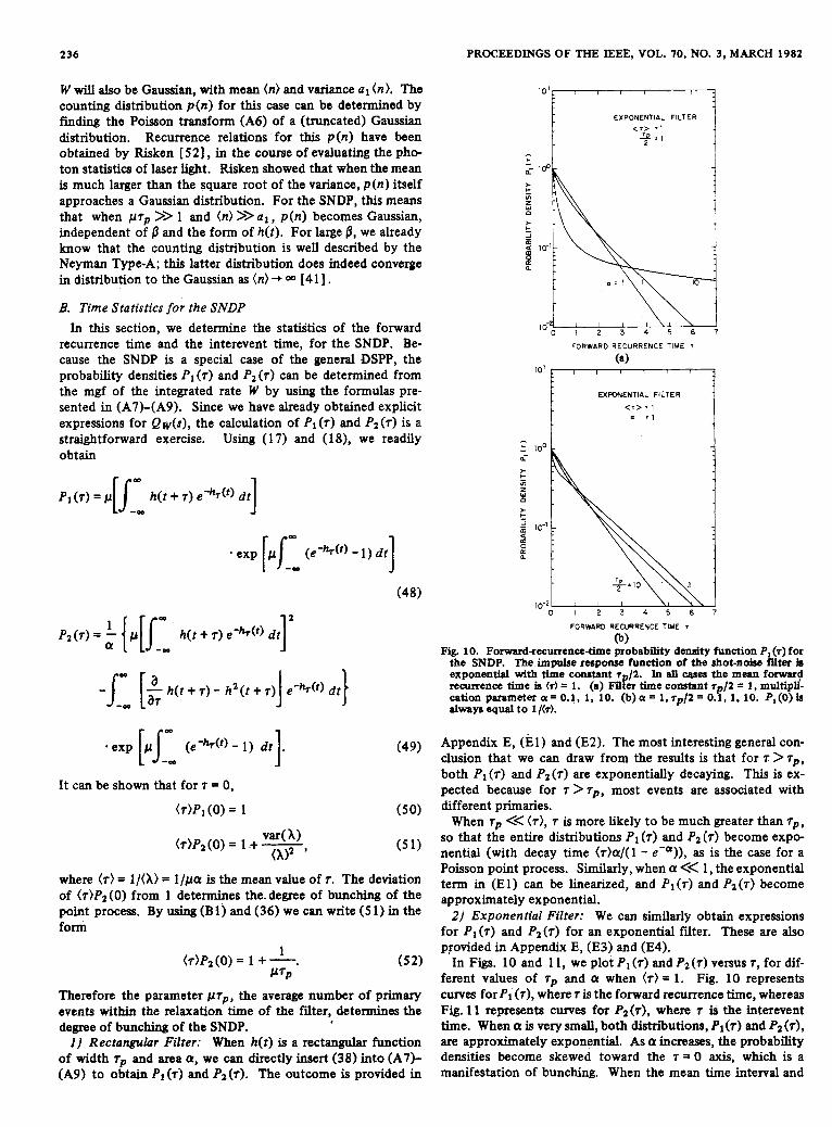
(b) Fig. 10. Forwardrecurrence-time probability density function P,(?) for

the SNDP. The impnlse response function of the shot-noise Nter is exponential with time constant 7 /2. In dl cases the mean forword recurrence time is (7) = I. (a) F ~ L time constant r /2 = 1, multipu: cation parameter u = 0.1, 1, 10. (b) a = l;rP/Z = O . f , 1, 10. P,(O) is always equal to 1 / ( A

Appendix E, (El) and (E2). The most interesting general conclusion that we can draw from the results is that for r > rP, both PI (7) and Pz (7) are exponentially decaying. This is expected because for 7 > T ~ , most events are associated with different primaries.

When T~ << ( r ) , 7 is more likely to be much greater than rP, so that the entire distributions P1(7) and PZ (7) become exponential (with decay time (7)a/( 1 - e-u)) , as is the case for a Poisson point process. Similarly, when a << 1, the exponential term in (El) can be linearized, and P1(7) and Pz(7) become approximately exponential.

2 ) Exponential Filter: We can similarly obtain expressions for PI(T) and Pz(7) for an exponential filter. These are also provided in Appendix E, (E3) and (E4).

In Figs. 10 and 1 1, we plot P1(7) and Pz(7) versus 7, for different values of T~ and a when ( 7 ) = 1. Fig. 10 represents curves for P1 (T), where 7 is the forward recurrence time, whereas Fig. 1 1 represents curves for Pz(7), where 7 is the interevent time. When a is verysmd, both distriiutions, Pi(7) and P2(?), are approximately exponential. As a increases, the probability densities become skewed toward the 7 = 0 axis, which is a manifestation of bunching. When the mean time interval and


l o ’ - is given by

INTER-EVENT TIME 1

EXPONENTIAL FILTER < r > = l

INTER-EVENT TIME I

@) Fig. 11. Interevent (pulseinterval) probability density function P2(7) for

the SNDP. The impulse response function of the shot-noise filter is exponential with time constant rP/2. In all cam the mean interevent time is ( 7 ) = 1. (a) Time constant rP/2 = 1, multiplication parameter c r = O . l , 1, 10. ( b ) a = 1,7p/2=0.1 ,1 , 10 .

(Y are held fixed, decreasing rP similarly skews the densities toward the T = 0 axis, as is evident from the figures.

IV. MULTIFOLD STATISTICS FOR THE SNDP A. Counting Statistics

The joint statistical properties of the number of counts { n i } in N time intervals [ t i , ti + T i ] , j = 1, 2, - * - , N , for an SNDP can be determined by using the properties of doubly stochastic Poisson processes. Once the multifold mgf of the integrated rates

tj+Tj

wj = I, X(t) d t , j = 1, 2, - . , N (53)

is determined, the multifold factorial moments <IIi,,ni!/ (ni - m i ) ! ) and the joint counting distribution p ( n l , n 2 , * . , nN) for { n i } can be determined by using (A12) and (A13). To determine the mgf of { W j } , we need the mgf of {X(t j )} . For a shot-noise process h(t), the multifold mgf is known ((B9)I. By generalizing the analysis presented in Section 111 to the multifold case, we can easily show that the mgf of { Wi}

N

where

hTj ( r ) =[” h ( t + t ’ ) d t ’ .

We can therefore determine the joint statistics of { n i } explicitly.

B. Correlation Function and Power Spectrum The simplest special case is N = 2. Setting T1 = T2 = T in

( 5 9 , and m l = mz = 1 in (A12), we obtain the correlation function between counts in time intervals T separated by a time delay T = tz - t l # 0,

G$’)(T) = ( n l n 2 ) = p z [II, h T ( X ) d l

+ PJ-; ~ T ( x ) ~ T ( T + x) d x , ( 5 6 )

where h T ( r ) is given by (17). By use of (171, we can rewrite the counting correlation function in the form

G ~ ) ( T ) = ( n Y + ( n ) $(T), T # 0. (57)

Here T T

$(7) = 9 &T + t ’ - t ) d r d t ’

where Z

f ( 7 ) =r h ( t ) h(t + 7) d r / [ l m h ( t ) d t ] ( 5 9 )

is a normalized version of the autoconelation function of h( t ) . For T = 0, Gf)(O) = (n’), which according to (21) and (25),

is

-OD

Note that $(O) = a1 , the excess Fano factor. For the usual example of an exponential impulse response function, h(r) = ( 2 a / T ~ ) exp ( - 2 t / r p ) , ( 5 8 ) - ( 6 0 ) yield

where

b = [cosh ( 2 8 ) - 11 /28 )a = 28/(e-28 + 28 - 1) ( 6 2 ) and 8 = TITp. The counting correlation function is therefore exponential. Similar results have been obtained by Vere-Jones and Davies [35].

238 PROCEEDINGS OF THE IEEE, VOL. 70, NO. 3, M A R C H 1982

When the sampling time T is much shorter than the time scale

4(r) = a T W , (63)

i.e., #(7) is proportional to t (7). The power spectral density !~~ (a ) of the process, represent-

ing fluctuations n( t ) - (n(t )> in the number of counts in an interval [ t, t + TI, can be determined by taking the Fourier transform of the autocovariance function c~,~)(T) - ( n ) 2 . his results in .an expression of the form

sAn(@) = (n> + ( n ) @(a) (64) where @(@) is the Fourier transform of #(r). For a Poisson process, the second term of (64) disappears, and S&(rco) = (n) . It is clear, therefore, that the second term represents excess noise. It is usual to define the relative excess noise as

of the filter rP, (58) becomes approximately

[sAn(a) - s&~n(a)l /s;n(a) = @(a). (65) For a short counting time (T<< rp) , equation (63) applies

and (59) gives

%a) = - I m J J ) 1 2 , T

(66) a where H(a) is the trahsfer function of the filter (i.e., the Fourier transform of h(t)) . For an exponential filter, the relative excess noise has a Lorentzian shape

@'(a) a T / [ 1 + a 2 < / 4 1, (67)

with an amplitude proportional to a and T . In many situations a point process is observed not by count-

ing, but rather by filtering the incoming pulses to generate a continuous signal, which we denote as dt). If such a filter has a rectangular impulse response of width T and unit area, then s ( t ) would be identical to n( t ) , the number of counts in an interval [0, TI. Therefore, the above results regarding counting statistics (including moments, correlation, and power spectral density) are also statistics of s( t ) . In a typical situation, when the point process represents the passage of electrons in a circuit, ( e / T ) n ( t ) represents the electric current. Here, e is the electronic charge, and T is the impulse response time of the circuit, when it is approximated by a rectangular function.

V. APPLICATIONS OF THE SNDP The mathematical description discussed to this point applies

to a broad variety of phenomena. In the following, we deal with a number of applications of special interest in electrical engineering and physics. In particular, we use the SNDP model for describing the following processes: A) the detection of scintillation photons created by nuclear particles; B) photomultiplier noise produced by ionizing radiation; C) cathodoluminescence; and D) X-ray radiography and electronography. The SNDP model will also be useful in studies of related areas such as image intensification, the detection of particles by means of devices such as avalanche photodiodes and electron multipliers, and visual perception.

A. Scintillation Photon Counting 1) Description of the Process: The detection of ionizing

radiation is often accomplished through a radiation-matter interaction in which a single highenergy particle produces a .shower of particles of lower energy. A case in point is the scintillation detector, which is a combination of a scintillation crystal (eo., NaI : T1, plastic) with a photomultiplier tube

~ ~ S S O N

cL PHOTON - OF LUMINESCENCE I W I Z I N G RATE OF PRODUCTION

~ PHOTON POISSON

*(, , - (OJl* 1 1 1 I I h l t l l r a t r r l

- EMISSION PHOTONS

- RADIATION

I ' I - - Fig. 12. Model for the photon point process generated by sciotiIl.tion radiation, cathoddumineacence, and photduminescence. O k m e the relation to Fig. 3 which is the mathematical model studied here.

[53]. Conditions for the validity of the SNDP in describing scintillation detection are that the incident primary ionizing particles (e.g., electrons, gammas, protons) be representable as a homogeneous Poison point process, and that each primary event have associated with it an impulse response function h(r) that directly governs the rate of production of Poisson optical photons.

A model for the physical process is illustrated in Fig. 12. It is seen to be identical in form to the block diagnun presented in Fig. 3, so that the resulting photon emissions form an SNDP. The function h ( t ) will often be approximately a decaying exponential, so that the counting and time statistics are given by (27), (44)-(47) and (El), (E3), (E4), respectively. The description is completely characterized by 1.1 and h( t ) and therefore, in this case, by three parameters: 1.1, the rate of the primary process; a, the multiplication parameter; and rp, the lifetime of the process of secondary event generation. If we perform photon counting, we must adjoin T, the counting time. It is clear from Section III-A3, that in the limit of counting times much longer than the exponential decay time, the counting distribution will reduce to the Neyman Type-A for arbitrary h ( t ) . It is often assumed in the literature, generally tacitly, that scintillation photon counting statistics are describable by the fiied multiplicative Poisson distribution; this provides an appropriate approximation only for T >> rP and a >> 1, however [41]. Of course, in those cases where the secondary events are not describable by a Poisson process, the SNDP is not the proper representation.

2) Experiment: A series of counting experiments of radioluminescence photons produced in glass has been recently carried out [50]. High energy 0- particles from a 9oSr-90Y equilibrium-mixture source irradiated the Coming 7056 glass faceplate of an EMR type 541N-01 photomultiplier tube from a distance of about 11.5 cm. The maximum 8- energies were 0.54 and 2.23 MeV for the %r and respectively, and the 0' flux was -8.2 X lo3 cm-2 s- l . External light was excluded. The photomultiplier anode pulses were passed through a discriminator and standardized. Unavoidable system dead time was -60 ns. The standardized pulses were counted during consecutive fixed counting intervals ( T = 400 ps) and the counts were recorded. The experiment was performed repeat- edly to obtain good statistical accuracy, and a histogram representing the relative frequency of the counts was constructed. The total duration of a run was about 4 min. In the particular experiment we illustrate, the observed mean count was 85.89 (this number was substantially higher than the mean dark count which could therefore be neglected) and the observed count variince was 429.58. The data are shown as the dots in Fig. 13. The solid curve represents the Neyman-Type A theoretical counting distribution with the count mean and variance fixed at the experimental values. It is clearly in accord with the data. When one assumes that rp << T (')R = l), (C3) yields an experimental multiplication parameter a = 4.0. A Poisson distribution with mean 85.89 (indicated by arrow) is plotted as the dashed curve in Fig. 13 ; clearly it bears no relation to the data.


I l l

- POISSON?’ ‘I NYMANTYPE-A- , - , I I I -

20 40 w eo 100 120 140 160

NUMBER OF CWNTS (n)

Fig. 13. Photon counting distribution p ( n ) versus number of photon counts n. Data (dots) represent radioluminescence photon registra- tions from the glass faceplate of a photomultiplier tube, induced by ’ O S - ”YP- rays. The counting time T = 400 w. The experimental

solid curve repredents the Neyman Type-A theoretical counting dik count mean and variance are 85.89 and 429.58, respectively. The

tribution with the same values of count mean and variance (a = 4.0).

shown aa the dashed curve. After Fig. 2 of the paper by Teich and The P o k o n distribution with mean 85.89 (indicated by arrow) k

Saleh [SO] .

Because the primary process in this case consisted of highenergy charged particles (electrons), Cerenkov radiation could have been produced in addition to luminescence radiation. However, even if a large number of photoelectrons were generated by the Cerenkov photons arising from a single particle, they would nevertheless appear as a single (large) photoelectron pulse since the Cerenkov radiation emission time is much shorter than the transit time in the photomultiplier. In the presence of kerenkov radiation, therefore, the (unmarked) total point process will include the primary as well as the subsidiary process.. An analysis of this union process will be presented at a later time, but it will be well characterized by the SNDP for a >> 1.

B. Photomultiplier Noise Induced by Ionizing Radiation In certain applications in which we wish to observe photon

arrivals by using a photomultiplier tube, e.g., in astronomy conducted at high altitudes or in space, the description provided above may be characteristic of the noise rather than of the signal. Viehmann and Eubanks [541,[551 have discussed sources of noise in photomultiplier tubes in the ionizing radiation environment of space. Such noise may arise from several mechanisms such as luminescence and Cerenkov radiation in the photomultiplier window; secondary electron emission from the window, photocathode, and dynodes; Bremsstrahlung in turn causing such secondary electron emission; cosmic-ray bursts; and, of course, thermionic emission dark current. These effects clearly degrade both the dynamic range and the photo- metric accuracy of low-light-level measurements, and therefore must be properly modeled. It is evident from the experimental results reported in the previous subsection that the SNDP provides a sound point of departure in modeling a number of these sources of noise. Luminescence will be the dominant source of noise in many applications.

C. Cathodoluminescence 1 ) Description of the Process: Cathodoluminescence is an

important process in which a beam of accelerated electrons incident on a luminescent material (e&, a phosphor) induces the emission of light [ 281, [ 291. It is the process responsible

1

‘i

e e m K)-so 5

10 15

UORYALIZED FORWARD RECURRENCE TIME r/(r>

Fig. 14. Dots represent the relative frequency of tb -e to the first cathodoluminescsnt photoelectron event for a YVO, :Eu3+ phosphor with the exciting electron energy fixed at 10.2 keV. The mean photon- counting rate wm 2.54 X lo4 s-’ and the mean dark counting rate

which represent the SNDP theoretical probability density function was 1.28 X 10’ 3-’. The solid curve is a plot of (El), @3), and (E4),

(T)P,(T) versus the normalized forward recurrence time T/(T) f a an exponentially decaying shot-noise pulse, with F = 39.7 w, a = 9.6,

retwxtc&. Data adapted from Fig. 6 of the paper by van Rijswijk and T /2 - 0.5 ma. Dark noise has been accounted for in the the*

1571.

for the television and oscilloscope image. Conditions for the validity of the SNDP in describing cathodoluminescence are that the electron beam reaching the sample be represented as a homogeneous Poisson point process, and that each primary event have associated with it an impulse response function h ( t ) that governs the rate of production of noninterfering Poisson optical photons. Cathodoluminescence may therefore be represented by the physical model in Fig. 12 if we simply replace the block labeled “Poisson ionizing radiation” by a block en- titled “Poisson electron beam.”

The counting statistics are then given by (27) and (28), whereas the time statistics are specified by (48) and (49). The description is completely characterized by 1.1 and h( t ) , and again, in the limit of counting times long in comparison with the time scale of h( t ) , the counting distribution reduces to the Neyman Type-A for arbitrary h ( t ) .

In the special case where the function h ( t ) is a decaying single- timeconstant exponential, each electron entering the sample induces an exponentially decaying flux of luminescence photons, so that the counting and time statistics will be given by (271, (44)-(47) and (El), (E3), (E4), respectively. These results are the same as those derived by van Rijswijk [ 56 1 , [ 5 71 by means of an entirely different method. It appears that van Rijswijk’s result can be used only for luminescence that decays precisely exponentially, whereas our general result will be valid for arbitrary h( t ) . In particular, we can easily account for the finite “decay” (rise) time of the luminescence emission.

2 ) Forward Recurrence-Time Measurements: The statistics for the time to the first cathodoluminescent photon arrival were experimentally measured by van Rijswijk [57] for a Yvo4 :Eu3+ phosphor and, more recently, by Timmermans and Zijlstra [ 581 for ZnS : Ag. In Fig. 14 we present the normalized forward recurrence time data (dots) for YV04 : Eu3+ obtained by van Ftijswijk [ 571 with an incident electron energy


W g 100

m 0

Y

FREOUENCY (Hz)

Fa. 15. Dofl reprasnt the experimental relative exc- noise in the photomultiplie mode ament for cathodolumineacenca from ZnS : Ag. The solid curve is a Lomtzian. Figure adapted €torn Fs. 3 of the paper by 'I2mmammr and Ziprtra [ 58 1.

of 10.2 keV. The mean photon counting rate was 2.54 X lo4 s-' and the mean dark counting rate was 1.28 X lo3 s-'. The solid curve is a plot of (El), (E3), (E4), which represent the normalized probability density for the theoretical forward recurrence time PI (7) for an exponentially decaying shot-noise pulse, with7 = 39.7 p, a = 9.6, and rP/2 = 0.5 m s . The effects of dark noise were not negligible in this w e and were accounted for in the solid cume (571.

3) Excess-Noise Specmtm Measurements: Intensity flue tuations for cathodoluminescence were fmt investigated by means of the spectral properties of excess noise in the phot* multiplier anode current [ 591, [ 601. The theoretical expression for the spectrum in the general case (viz., for arbitrary h(t) and arbitrary T) was derived in Section IV-B. The result for an exponentially decaying shot-noise pulse, in a form appropriate when measurements are made by a real-time spectrum analyzer, is presented in (67). Previous calculations were carried out only for purely exponentially decaying luminescence, which leads to the characteristic Lorentzian spectral shape.

Recent excess-noise measurements were performed by van uswijk [57] for W04:Eu3+ and by Timmermans and Zijlstra [58] for ZnS:Ag. In Fig. 15 we present ZnS:Ag experimental relative excess noise as a function of frequency (dots) obtained by Timmermans and Zijlstra. The solid curve is a Lorentzian which provides an excellent fit to the data, providing confirmation of the exponential decay shape and the luminescent-center lifetime.

D. X-Ray Radiography and Electronography The recording of X-rays (or 7-rays) on a photographic emul-

sion involves a cascade of two processes [ a l l . The absorption of high-energy photons results in the emission of electrons (through the photoelectric effect, Compton scattering, or the formation of electron-positron pairs). The emitted electrons then traverse the emulsion, rendering a random number of silver halide grains developable. The higher the photon energy, the larger the average number of developable grains per photon [61]. It is a common observation in industrial radiography, that the higher the photon energy, the greater the graininess of the exposed fii. This is a direct result of the exposure of a larger average number of grains per photon, and their clustering around that photon. With commercially available X-ray films this effect is easily visible to the naked eye [ 6 1 1 .

It is apparent that the SNDP can serve as a simple model to account for this multiplicative cascade of events (assuming that other complex phenomena which may occur in the emulsion can be ignored). The primary process is then the random electrons which, because of the local Poisson nature of the incident photons in a region of f i e d irradiance, can be reason- ably assumed to form a Poisson point process of rate p per unit area. These events are then spatially filtered, Le., they are spatially spread, as they are transmitted through, and scattered by, the emulsion. The spread in energy of each primary electron then renders a random number of the grains in its path (on the average a) developable. The developable grains form the secondary process, and if this number is Poisson, the SNDP ensues. Note that here, time is replaced by space, and the SNDP is a spatial point process.

The detection of electron beams (in such fields as electron microscopy, electron diffraction, and Bray dosimetry) may be similarly described [61 I, (621.

The photographic detection of both electrons and X-rays obey the singlehit theory [6 1 1 , which means that a single detected particle is capable of rendering one or more silver halide grains developable. An important property of the SNDP is the fact that the variance-to-mean ratio (the Fano factor) is larger than one and is independent of the rate of the primary events (the intensity of the electron image). The multiplication parameter a, which determines the Fano factor, is larger than one for single-hit processes.

In radiography, X-ray images may also be detected by use of intensifying screens. X-ray radiation illuminates a fluorescent screen, which emits visible photons that are recorded on a photographic emulsion. An X-ray photon impinging on the fluorescent screen results in the emission of a random number of light photons. These spread as they propagate to the phot+ graphic emulsion, forming a patch of illumination with a spatial distribution h(x , y ) , which is the point-spread function or the spatial impulse response function. If the incoming X-ray radiation is of uniform irradiance p photons per unit area, its photons would be distributed according to a homogeneous Poisson process of rate p. If we postdate that A , the number of light photons per X-ray photon, also has a Poisson distribution of mean value ( A ) = a, then the light photons arriving at the emulsion will obey an SNDP, with parametersp, a, and h(x , y) .

It follows, then, that the light photons should exhibit spatial clustering. Such clustering has been observed experimentally, and is often referred to as quantum mottle. Indeed Kemper- man and Trabka [631 have recently used the same model to describe the first- and second-order statistics of exposure fluctuations in the recording of X-ray images using intensifying screens.

VI. CONCLUSION Thorough consideration has been given to the counting and

time statistics for the SNDP. This process provides a natural description for phenomena involving the random multiplication (or reduction) of Poisson point events with a random time delay. The SNDP is a particular Neyman-Scott cluster process. The model has been applied to a number of important problems in electrical engineering, physics, and optics, including cathodoluminescence, photomultiplier-tube luminescence noise induced by ionizing radiation, the photoncounting scintillation detection of nuclear particles, X-ray radiography, and electronography. There are other singleatage random multiplication processes, involving random delay, for which this model provides a ready solution.

The model could be extended and strengthened in a number of ways. In this concluding section, we point to various restric-


tions that have been implicitly and explicitly imposed on the mathematical formulation, and discuss ways in which these restrictions can be relaxed.

The primary Poisson point process was taken to be homogeneous (HPP) and therefore stationary (see Fig. 3). Physical situations in which primary events are nonstationary also occur, and it is of interest to determine the statistical properties of the resultant process. This is necessary, for example, for studying cathodoluminescence when the exciting electron beam is pulsed. Another example that presents itself is the behavior of the neural discharge recorded from the mammalian retinal ganglion cell [64] excited by a brief pulse of light. We have recently solved for the counting distribution and the probability density function for the waiting time to the first event [ 651. It is quite interesting that the counting distribution reduces to the Neyman Type-A when the rate is a pulse of short duration (7, << rp + T ) . Spatialinhomogeneities, correlations, and selection can also be important, so that it will be worth- while to consider the addition of SNDP’s and to extend the formulation to more than one dimension.

As is usual for the Neyman-Scott process, we have assumed that primary events are excluded from the final point process. A modified model may be constructed in which the resultant process is the union of the SNDP with the primary process. The statistics of the combined point process cannot be obtained by simple convolution because of the statistical dependence between primary and subsidiary events. In the long-counting- time limit, when the SNDP yields the Neyman Type-A counting distribution, it can be shown that the counting statistics associated with the combined process is the Thomas distribution [41], [66] .

Moving to the linear filter in Fig. 3, we have tacitly assumed throughout that h ( t ) is a deterministic impulse response function. Gilbert and Pollak [45] have shown that if the filter h ( t ) contains a random parameter, then an equivalent completely deterministic impulse response function h’(t) can always be found that generates h(t) with identical statistics. In particular, if h ( t ) = h 0 ( t / T p ) , where 7 p is random, h’(t) = ho(t/(17,1)). This is an important result because it tells us that the analysis we have carried out applies also when the linear filter is not deterministic. In the context of cathodoluminescence, for example, not only can we ascribe an arbitrary time course to the phosphorescence by choosing h ( t ) appropriately, but we can also permit h ( t ) to contain a stochastic parameter. Indeed it is likely that local field inhomogeneities in a real phosphor will create some degree of randomness in T ~ .

Again examining Fig. 3, we see that the shot noise h(t) provides the rate for this second Poisson process. Our model can be modified to permit this second Poisson process to be self- excited, thereby allowing for aftereffects triggered by past events [ 3 ] . This modification will be immediately useful for calculating the effects of phenomena such as dead time (abso- lute refractoriness) and sick time (relative refractoriness). We have recently derived the interevent-time statistics for the SNDP with 1-memory recovery, and examined examples of their use in scintillation detection and vision [67] . A solution has also been obtained for the count mean and variance for an arbitrary dead-time-modified DSPP. These expressions have been experimentally verified for @--induced radioluminescence photons produced in several transparent materials, in the presence of system dead time [68] . l For large counting

The proper result for the variance-to-mean ratio for an SNDP with a ‘We note that the dashed curve shown in Fig. 3 of [ 6 8 ] is incorrect.

rectangular impulse response function, in the absence of dead time, is given by (22), (23), and (39b) above. - This curve does indeed lie every-

times, we also showed that the experimental photon-counting distributions were well described by the Neyman Type-A theoretical distribution, both in the absence and in the presence of dead time [681.

Given an SNDP Cf(t) in Fig. 3), we can easily account for the effects of a statistically independent Poisson point process representing, for example, broadband background light in a photomultiplier ‘tube. The counting statistics for the superposition process can be simply determined by numerical convolution. An interesting case arises in the context of photomultiplier dark noise. Such dark counts can be considered to arise from a combination of photocathode and dynode thermionic emission, describable by the HPP, and multiplication noise. We have recently analyzed the experimental counting statistics for photomultiplier dark noise, and found it to be consistent with this model over a rather broad range of counts [69] . A related approach has been found to be useful for describing the detection of light by the human visual system at threshold [ 701.

We should, perhaps, say a few words about branching (cascade) processes, in which each subsidiary event generates its own cluster, and so on. This kind of nesting may be referred to as higher-order clustering; in this framework, the SNDP is first-order clustered. A generalization of the SNDP to allow for nesting will be valuable for deriving the precise counting and time statistics for electron devices that involve more than one stage of random multiplication and random time delay. Examples are the avalanche detector and the electron multiplier. We have recently analyzed some problems of this type [ 7 1 ] .

Finally, we point out that the statistical behavior of the clustered processes considered here is sufficiently unique that one may conceive of innovative signal processors and receivers specifically designed to enhance such signals (or discriminate against such noise). Calculations of the performance charac- teristics of such devices (detection, discrimination, estimation) will have to be carried out, of course, to ascertain the value of any such proposed scheme. In the meantime, we have experimentally shown that dead time does selectively discriminate against such clusters [68] .

APPENDIX A GENERAL PROPERTIES OF THE DSPP

For a DSPP with stochastic rate h(t), the counting statistics (statistics of n) can best be described in terms of the statistics of the random variable

w = lT h(t) d t

which represents the integrated rate of events [3] , [ 241, [ 261 , [27]. The moment-generating function of n is related to that of W by [27]

where Qw(s ) = ( e -WS) is the mgf of the random variable W. The factorial moments =(e)

n - m ) !

and the probability distribution p ( n ) , can be computed by use

where above the solid curves shown in [ 6 8 , figure 31, thereby con- fuming that the introduction of dead time always produces a decrease in the variance-to-mean ratio, as intuitively expected.

242 PROCEEDINGS OF THE B E E , VOL. 70, NO. 3, MARCH 1982

of the formulas [27]

Alternatively, p ( n ) can be determined from the Poisson transform of P( W )

P( W ) d W. n!

Statistics of the times of occurrence of the events of a DSPP can also be determined from the mgf of W. If PI(?) and Pz(7 ) represent the probability density functions for the forward recurrence time (time from an arbitrary point to the first event) and the interevent time, respectively, then [ 31 , [ 271

where

~ o ( T ) = Q w ( l > = P ( O ) , (A91

(X) is the mean rate of events, and p ( 0 ) is the probability of zero counts in the interval IO, T I . The key to determining the singlefold statistics of the DSPP therefore lies in the deter- mination of the moment-generating function Q w ( s ) of its integrated rate W.

Joint statistics of the number of events (nj) in N time intervals [ t i , t j + T i ] , j = 1,2, * * * , N , can also be obtained from the multifold mgf

of the integrated rates

'r' Tj wj = X(t) d t . (A1 1)

9 The factorial moments are given by

and the joint counting distribution is

p(n1, * * , nN)

APPENDIX B GENERAL PROPERTIES OF SHOT NOISE

The statistics of shot noise X(t) are well known [ 161, [45] - [47] ; they aresummarized here for subsequent use.

A . Singlefold Statistics The f i t - , second-, and third-order moments are, respectively,

(X( t ) ) = p I- h ( y ) d y = p a

OD 00

(X3(t)> =p3a3 + 3pz h 2 ( y ) d y + p h'(y) dy. (Bl) 0

The moment-generating function is

Qh(s) = = exp { p e: - 11 d t } . (B2)

The probability density function P(h) can be determined by solving the integral equation [45]

hP( X) = p 1- PIX - h( t ) l h ( t ) dt . (B3) -00

Explicit solutions for this equation are known in only few cases, as indicated below.

1) Rectangular Filter: The filter

elsewhere

corresponds to a fixed-multiplicative probability density

(prp k e - M 7 ~

k! P( A) = 6(h - kh), k = 0, 1, 2, a * * , (BS)

i.e., X takes the discrete values 0, b, 2 b , - * - , kb, * * where k has a Poisson distribution of mean prp.

2) Special Filter with Logarithmic Singularity and Expo- nential Tail: Another filter with rather simple properties is that described by the impulse response function [45 I

where E;'(X) is the inverse of the exponential integral

(B 7)


B. Multifold Statistics The multifold moment-generating function is [46]

In particular, the twofold mgf is given by

r P -

and the correlation function is written as

APPENDIX C PROPERTIES OF THE NEYMAN TYPE-A DISTRIBUTION

The Neyman Type-A distributed random variable n of parameter a has an mgf [40], [41], [49]

Its factorial moments are given by the recurrence relation provided in (1 9), with

al = a 1 . (C2)

In particular, the variance is

var(n)=(l + a ) ( n > (C3)

so that the excess Fano factor al is equal to a. The Neyman Type-A probability distribution p ( n ) is determined from the recurrence relation in (27). The coefficients Cl are

c1= - I !

so that (27) becomes [40]

n a 1 ( n + I ) p ( n + 1) = (n> e-' - p ( n - I )

1 =o I !

Note that when a + 0, (C5) reduces to

(n + l ) p ( n + 1) = ( n > p ( n ) , p ( 0 ) = e-(n) (C6)

which is the recurrence relation for the ordinary Poisson distribution. This same result may be obtained by letting a + 0 in (Cl). This leads to Q,(s) = exy [(n> ( e -S - l ) ] , the mgf of the Poisson distribution.

APPENDIX D COUNTING STATISTICS FOR SOME SPECIAL FILTERS IN

THE LIMIT OF SHORT COUNTING TIME A . Rectangular Filter

When the impulse response function is rectangular of area a and width r P , each event of the primary homogeneous Pois- son process initiates a rectangular pulse. Within the time interval of that pulse, secondary Poisson events occur at the rate pa/rp per second. With h ( t ) rectangular, (33) yields

where the mean number of counts (n) registered in the time interval T is

(n> = paT, (D2)

and where

0 = T I T p . (D3)

Using (A2) we then amve at Q n ( s ) , which turns out to be

en($) =exp - {exp [a/3(e-s - l)] - 1}) . (D4) (:; This is precisely the rngf of the Neyman Type-A distribution of parameter a0 (see (C1)).

We conclude that the shot-noise-driven Poisson point process results in the Neyman Type-A counting distribution when the impulse response function of the filter is rectangular in shape, and the counting time is very short.

B. Exponentially Decaying Filter

(2a/rP) exp (-2t/rp), (33) gives When h ( t ) is an exponentially decaying function, h(t) =

where again the mean count (n> = paT and 0 = T I T p . The factorial and central moments of n are given by (19)-(22), with

Comparing these moments with those derived for the rectangular filter (viz., those of the Neyman Type-A distribution) we see that, for the same variance, the third central moment (and the skewness defiied by (26)) is larger in the exponential case than in the rectangular case.

The probability distribution p ( n ) is given by (27) in con- junction with the coefficients C1 from (28), which are now

Here 7(Z+ 1, x ) is the incomplete gamma function, which may be computed from the series

y(Z+ 1, x ) = I ! 1 - e -x x ' /k! ] . (D8) 1

[ k=O

244 PROCEEDINGS O F THE IEEE, VOL. 70, NO. 3, MARCH 1982

Also

Again, for vanishing Tor a, the counting distribution becomes Poisson.

C. Special Filter with Logarithmic Singularity and Exponential Tail

This fiter, described by (B6), comsponds to shot noise with a rate h( t ) characterized by the gamma probability density function (B8). The integrated intensity W AT wiU also have a gamma density with mean ( W) and parameter M = prp. In this case, we obtain the counting distribution p ( n ) by using the Poisson transform specified in (A6), since it is well known that the Poisson transform of the gamma density is the nega- tive binomial distribution, as was first shown by Greenwood and Yule 1721 :

p ( n ) = ( n , )/(! +$y (1 +z)M. (D10) n + M - 1

This distribution also turns out to provide a good approximation for the photocounting detection of multimode chaotic light of arbitrary spectrum; in that case M represents the number of degrees of freedom of the chaotic light [ 81, [ 121, [ 241, [27], [SO], [73], [74]. This is to be distinguished from the degrees-of-freedom parameter R for the shot-noise light considered here [ SO]. The factorial moments are

The variance is given by [SO]

var ( n ) = ( n ) + ( d Z / M = (1 + ab) (n ) (D 12)

so that the excess Fano factor for this distribution is again u l = ap. The SNDP is, in this example, equivalent to an inhomogeneous Polya process [ 21 , [ 75 I .

APPENDIX E

AND EXFQNENTIAL FILTERS

time and the interevent time are, respectively,

-1

TP

rpa2

For a rectangular filter of width rp and area a

TIME STATISTICS FOR AN SNDP WITH RECTANGULAR

The probability density functions for the forward recurrence

P1(r) = -R‘d exp ( R d )

P2(r) = - (R” + R ” d ) exp ( R d ) . (El ) 1

e - “ * ( a - ax - 2)- (a+ax - 2), X Q i

e - ” ( a x - a - 2 ) - ( a + a x - 2 ) , x > l R = {

R ’ = { e -axa( 1 - a + ax) - a, a(e-“ - 11,

x Q 1

x 2 1

X Q l

x 2 1

For an exponential filter of time constant rp/2 and area a,

with

and = 2r/rp.

ACKNOWLEDGMENT It is a pleasure to thank K. Matsuo for valuable suggestions.

REFERENCES

[ 1 ] E. Parzen, Stochastic Proce&ws. San Francisco, CA: Holden-

[ 21 F. A. Haight, Handbook of the Poiwon Distribution. New York: Day, 1962.

[ 3 ] D. Snyder, Random Point Processes. New York: Wlley-Inter- Wiley, 1967.

[ 4 ] D. R. Cox, “Some statistical methods connected with series of science, 1975.

[ 5 ] D. A. Darling and A.J.F. Siegert, “A systematic approach to events,” J. Roy. Stat. SOC., ser. B, vol. 17, pp. 129-164, 1955.

a class of problems in the theory of noise and other random phenomena-Part I,” IRE Trans. Inform. Theory, vol. IT-3, pp.

[6 ] A.J.F. Siegert, “A systematic approach to a class of problems in the theory of noise and other random phenomena-Part 11, Examples,” W E Trans. Inform. Theory, vol. IT-3, pp. 38-43,

[ 7 ] E. M. Purcell, “Correlation in the fluctuations of two phot* 1957.

electric currents evoked by coherent beams of light,” Nature,

[ a ] L. Mandel, “Fluctuations of photon beams: The distribution of the photo-electrons,” Proc. Pbys. Soc., vol. 74, pp. 233-243, 1959.

[ 9 ] R. J. Glauber, “The quantum theory of optical coherence,” Phys. Rev., vol. 130, pp. 2529-2539, 1963.

[ 101 R. J. Glauber, “Coherent and incoherent states of the radiation field,”Phys. Rev., vol. 131, pp. 2766-2788, 1963.

[ 1 1 ] P. L. Kelley and W. H. Kleiner, “Theory of electromagnetic field measurement and photoelectron counting,” Phys. Rev., vol 136,

[12] J. Peiina, “Superposition of coherent and incoherent fields,”

[ 131 G. Bddard, “Photon counting statistia of Gaussian light,” Phys.

[ 141 S. Karp and J. R. Clark, “Photon counting: A problem in classical noise theory,” IEEE Trans. Inform. Theory, vol. IT-16, pp. 672- 680, 1970.

[ 151 0. Macchi, “Distribution statistique des instante d’dmission des photodlectrons d’une l u m i h thermique,” C. R. Acad. Sci. (Paris),

[ 161 S. 0. Rice, “Mathematical analysis of random noise,” Bell Syst. Tech. J., vol. 23, pp. 1-51, 1944; vol. 24, pp. 52-162, 1945 [Reprinted in Selected Papers on Noise and Stochastic Processes,

[ 171 M. Kac and A.J.F. Siegert, “On the theory of noise in radio re- N. Wax, Ed. New York: Dover, 1954, pp. 133-2941.

ceivera with square-law detectors,” J. Appl. Phys., vol. 18, pp.

[ 181 D. Slepian, “Fluctuations of random noise power,” Bell Sys t Tech. J. , vol. 37, pp. 163-184, 1958.

[ 191 W. J. McGill, “Neural counting mechanisms and energy detection in audition,” J. Math. Aychol. , vol. 4, pp. 351-376, 1967.

32-36, 1957.

vOI. 178, pp. 1449-1450, 1956.

pp. A316-A334,1964.

Phys. Lett., vol. 2 4 4 pp. 333-334, 1967.

Rw.,vo~. 151, pp. 1038-1039, 1966.

VOI. A272, pp. 437-440, 1971.

383-397, 1941.


[20 ) P.A.W. Lewis, “Recent results in the statistical analysis of univariate point proceses,” in Stochastic Point Procemes: Statistical Analysis, Theory, and Applications, P.A.W. Lewis, Ed. New York: Wiley-Interscience, 1972, pp. 1-54.

[ 2 1 ] A. J. Lawrance, “Some models for stationary series of univariate events,” in Stochastic Point Processes: Statistical Analysis, The- ory, and Applications, P.A.W. Lewis, Ed. New York: Wiley- Interscience, 1972, pp. 199-256.

[22] D. J . Daley and D. Vere-Jones, “A summary of the theory of

sis, Theory, and Applications, P.A.W. Lewis, Ed. New York: point processes,” in Stochastic Point Processes: Statistical Analy-

Wiley-Interscience, 1972, pp. 299-383 [23] L. Fisher, “A survey of the mathematical theory of multidimen-

sional point processes,” in Stochastic Point Processes: Statistical Analysis, Theory, and Applications, P.AW. Lewis, Ed. New York: Wiley-Interscience, 1972, pp. 468-513.

(241 J. Peiina, Coherence of Light. London, England: Van Nostrand- Reinhold, 1972.

[ 2 5 ] C. W. Hehtrom, Quantum Detection and Estimation Theory. New York: Academic, 1976.

[ 26) J. Grandell, Doubly Stochastic Poisson Processes. Berlin/Heidel- berg/New York: Springer-Verlag, 1976.

[27 ] B.E.A. Saleh, Photoelectron Statistics. Berlin/Heidelberg/New York: Springer-Verlag, 1978.

(281 H. W. Lwerenz, Introduction to Luminescence of Solids. New York: Wiley, 1970.

[29 ] S. Larach and A. E. Hardy, “Cathode-ray-tube phosphors: Prin- ciples and applications,” Proc. ZEEE, vol. 61, pp. 915-926, 1973.

[ 301 S. M. Sze, Physics of Semiconductor Devices. New York; Wiley, 1981.

[ 31 ] A. van der Ziel, Noise in Measurements. New York: Wiley- Interscience, 1976.

[32 ] D. Vere-Jones, “Some applications of probability generating functionals to the study of input-output streams,” J. Roy. Srat.

(331 K. M. van Vliet and L. M. Rucker, “Noise associated with reduc- SOC., ser. B.,vol. 30, pp. 321-333, 1968.

tion, multiplication and branching processes,” Physica, vol. 95A, pp. 117-140, 1979.

[ 341 M. S. Bartlett, “The spectral analysis of two-dimensional point processes,” Biometriku, vol. 51, pp. 299-311, 1964.

[ 3 5 ] D. Vere-Jones and R. D. Davies, “A statistical survey of earthquakes in the main seismic region of New Zealand, Part 11. Time series ana1ysis;’N.Z.J. Geol. Geophys.,vol. 9, pp. 251-284,1966.

(361 1. Neyman and E. L. Scott, “A statistical approach t o problems

[ 3 7 ] I . Neyman and E. L. Scott, “Processes of clustering and appli- of cosmology,” J. Roy. Stat. SOC., ser. B, vol. 20, pp. 1-43, 1958.

cations,” in Stochastic Point Processes: Statistical Analysis, The- ory, and Applications, P.A.W. Lewis, Ed. New York: Wiley-

[38 ] R. E. Burgess, “Homophase and heterophase fluctuations in semi- Interscience, 1972, pp. 646-681.

conducting crystals,” Dis. Faraday SOC., vol. 28, pp. 151-158, 1959.

(391 L. Mandel, “Image fluctuations in cascade intensifiers,” Brit. J.

[40 ] 1. Neyman, “On a new class of ‘contagious’ distributions, appli- cable in entomology and bacteriology,” Ann. Math. Stat., vol. 10,

[41] M. C. Teich, “Role of the doubly stochastic Neyman Type-A and Thomas counting distributions in photon detection,” AppJ. Opt.,

[42 ] D. Vere-Jones, “Stochastic models for earthquake occurrence,” J. Roy. Stat. SOC., ser. B, vol. 32, pp. 1-62, 1970.

[43 ] M. S. Bartlett, “The spectral analysis of point processes,” J. Roy. Stat. SOC., ser. B, vol. 25, pp. 264-296, 1963.

[44 ] P.A.W. Lewis, “A branching Poisson process model for the analysis of computer failure patterns,” J. R o y . Star. SOC., ser. B, vol.

[45 ] E. N. Gilbert and H. 0. PolIak, “Amplitude distribution of shot

[46 ] A. Papoulis, Probability, Random Variables, and Stochastic Pro- noise,” Bell Syst. Tech. J. , vol. 39, pp. 333-350, 1960.

(471 B. Picinbono, C. Bendjaballah, and J. Pouget, “Photoelectron cesses. New York: McGraw-Hill, 1965.

[48 ] W. Feller, “On a general class of ‘contagious’ distributions,” shot noise,” J. Moth. Phys.,vol. 1 1 , pp. 2166-2176, 1970.

Annu. Math. Stat., vol. 14, pp. 389-400, 1943. [491 H. Grimm, “Tafeln der Neyman-Verteilung Type-A,” Biometrische

[SO] M. C. Teich and B.E.A. Saleh, “Fluctuation properties of multi- Zeitschrift, vol. 6 , pp. 10-23, 1964.

plied-Poisson light: Measurement of the photon-counting distribution for radioluminescence radiation from glass,” Phys. Rev. A ,

Appl, Phys., V O ~ . 10, pp. 233-234, 1959.

pp. 35-57, 1939.

V O ~ . 20, pp. 2457-2467, 1981.

26, pp. 398-456, 1964.

VOl. 24, pp. 1651-1654, 1981. M. C. Teich and H. C. Card, “Photocounting distributions for exponentially decaying sources,” Opt. Letters, vol. 4, pp. 146- 148, 1979. H. Risken, “Statistical properties of laser light,” in Progress in Optics, vol. VIII, E. Wolf, Ed. Amsterdam, The Netherlands:

J. B. Birks, The Theory and Practice of Scintillation Counting. Elmsford, New York: Pergamon, 1964. W. Viehmann and A. G. Eubanks, “Noise limitations of multiplier phototubes in the radiation environment of space,” NASA Tech. Note D-8147, Goddard Space Flight Center, Greenbelt, MD, Mar. 1976. W. Viehmann, A. G. Eubanks, G. F. Pieper, and J. H. Bredekamp, “Photomultiplier window materials under electron irradiation: Fluorescence and phosphorescence,” Appl. Opt., vol. 14, pp.

F. C. van Rijswijk, “Photon statistics of characteristic cathodoluminescence radiation. I. Theory,” Physica, vol. 82B, pp. 193- 204, 1976. F. C. van Rijswijk, “Photon statistics of characteristic cathodoluminescence radiation. 11. Experiment,” Physica, vol. 82B, pp. 205-215, 1976. J. Timmermans and R.J.J. Zijlstra, “Photon-counting statistics of cathodo-luminescence light emitted by ZnS :Ag,” in Noire in Physical Systems, D. Wolf, Ed. Berlin/Heidelberg/New York: Springer-Verlag, 1978, pp. 42-48. T. M. Chen and A. van der Ziel, “Noise in cathodoluminescence light,” IEEE Trans. Electron Devices, vol. ED-12, pp. 489-493, 1965. H. M. Fijnaut and R.J.J. Zijlstra, ‘ Noise in cathodoluminescence radiation from a (CaMg)(Si03)2-Ti phosphor,’’ J. Phys. D. AppJ.

C.E.K. Mees and T. H. James, The Theory of the Photographic Process, 3rd ed. New York: MacMillan, 1966, ch. 10. S. Jeffers, “On the linearity of electronography,” Ashon. Astro- phys., vol. 92, pp. 196-199, 1980. J.H.B. Kernperman and E. A. Trabka, “Exposure fluctuations in model photographic emulsions. 11. Statistics due to intensifying screens,”Photogr. Sci. Eng.,vol. 25, pp. 108-111, 1981. H. B. Barlow, W. R. Levick, and M. Yoon, “Response t o single quanta of light in retinal ganglion celh of the cat,” Vision Res., vol. 1 1 , supplement 3, pp. 87-101, 1971.

tionary Neyman-Scott cluster process,” submitted for publication. B.E.A. Saleh and M. C. Teich, “Statistical properties of a nonsta-

in ecology,” Biomem’ka, vol. 36, pp. 18-25, 1949. M. Thomas, “A generalization of Poisson’s binomial limit for use

M. C. Teich and B.E.A. Saleh, “Interevent-time statistics for shot-

North-Holland, 1979, pp. 239-294.

2104-2115, 1975.

Phys., V O ~ . 3, pp. 45-53, 1970.

noise-driven self-exciting point processes in photon detection,”

68) B.E.A. Saleh, J. Tavolacci, and M. C. Teich, “Discrimination of J. Opt. SOC. Amer., vol. 71, pp. 771-776, 1981.

shot-noise-driven Poisson processes by external dead time: Appli- cation t o radioluminescence from glass,” ZEEE J. Quant. Elec- tron.,vol. QE-17, pp. 2341-2350, 1981.

691 M. C. Teich and B.E.A. Saleh, manuscript in preparation, 1982. 701 M. C. Teich, P. R. Prucnal, G. Vannucci, M. E. Breton, and W. J.

McGill, “Multiplication noise in the human visual system at threshold: 1. Quantum fluctuations and minimum detectable energy,” J. Opt. SOC. Amer., vol. 72, Apr. 1982; P. R. Prucnal and M. C. Teich, “Multiplication noise in the human visual system at threshold: 2. Probit estimation of parameters,” Biol. Cybern., vol. 43, pp. 87-96,1982; M. C. Teich, P. R. Prucnal, G. Vannucci, M. E. Breton, and W. J . McGill, “Multiplication noise in the human visual system at threshold: 3. The role of non-Poisson quantum fluctuations.” submitted for Dublication. 1982.

(711 K. Matsuo, B.E.’A. Saleh, and hi. C. TGch, “Cascaded Poisson

[72 ] M. Greenwood and G. U. Yule, “An inquiry into the nature of proceses,” submitted for publication, 1982.

with particular reference to the occurrence of multiple attacks frequency distributions representative of multiple happenings

of disease or of repeated accidents,” J. Roy. Stat. SOC., ser. A,

[73] G. Bddard, J. C. Chang, and L. Mandel, “Approximate formulas for photoelectric counting distributions,” Phys. Rev., vol. 160,

[74 ] M. C. Teich and W. J. McGill, “Neural counting and photon counting in the presence of dead time,” Phys. Rev. Lett., vol. 36, pp. 754-758, 1473, 1976.

[ 751 A. T. Bharucha-Reid, Elements of the Theory of Markov Processes and Their Applications. New York: McGraw-Hill, 1960.

, ~. ._

V O ~ . 83, pp. 255-279, 1920.

PP. 1496-1500, 1967.

proceedings of the ieee, vol. 70, no. 3, march...

Documents