proceedings of gt2009 asme turbo expo 2009: power for …

Copyright © 2009 by ASME 1

Proceedings of GT2009

ASME Turbo Expo 2009: Power for Land, Sea and Air

June 8-12, 2009, Orlando, Florida, USA

GT2009-59590

Overspray Fog Cooling in Compressor using Stage-Stacking Scheme with Non-Equilibrium Heat Transfer Model for Droplet Evaporation

Jobaidur R. Khan and Ting Wang

Energy Conversion & Conservation Center University of New Orleans

New Orleans, LA 70148-2220, USA

ABSTRACT

The inlet fog cooling scheme has been proven as an economic

and effective means to augment gas turbine output power on hot or

dry days. A previous paper developed a stage-by-stage wet-

compression theory for overspray and interstage fogging using the

equilibrium droplet evaporation model with given compressor and

blade configurations. This paper extends the previous work by

including the non-equilibrium droplet heat transfer model.

An 8-stage, 2-D compressor airfoil geometry and stage settings

at the mean radii are employed. Eight different cases including

saturated fogging, overspray with different droplet sizes with both

equilibrium and non-equilibrium heat transfer models have been

investigated and compared. The results show saturated fogging

increases the pressure ratio and reduces the compressor power

consumption; however, overspray actually increases both the specific

and total compressor power consumption. Non-equilibrium method

differs from the equilibrium method due to the change of evaporation

rate. Droplet size doesn't play a role in equilibrium approach, but

plays a major role in affecting the result in the non-equilibrium case.

For small droplet size of 10 µm, the droplet evaporation rate is fast,

so the non-equilibrium method predicts close results as the

equilibrium method. Larger droplets lead to slower evaporation,

reduction of pressure ratio, and less effective compressor

performance than the smaller droplets. Equilibrium method predicts

that wet compression increases axial velocity, blade inlet velocity,

incidence angle, and tangential component of velocity. Non-

equilibrium methods predict a similar trend except with lesser

increments as the droplet size increases. In the present study, the

equilibrium method predicts that all the water droplets evaporate

completely at the end of stage 3, while the non-equilibrium approach

predicts that the completion of evaporation delays, but all droplets

completely evaporate in the compressor except the biggest droplets

(30µm). Saturated fogging increases air density; however, both

equilibrium and non-equilibrium methods predict that overspray wet

compression actually reduces air density in the earlier 70% of the

compressor. Non-equilibrium predicts small droplets relax the load in

the earlier stages but increases the load in the later stages. Larger

droplets show less load changes. Detailed stage-to-stage performance

and property value changes are analyzed and discussed in this study.

NOMENCLATURE A Surface Area

d Droplet Diameter (µm)

D Mass Coefficient of Diffusion (m²/s)

D.A. Dry Air

Cp Specific Heat (kJ/kg.K)

GT Gas Turbine

h Heat Transfer Coefficient (W/m².K)

hfg Latent Heat of Evaporation (kJ/kg)

k Thermal Conductivity (W/m.K)

L Blade Chord Length

m Mass (kg)

Nu Nusselt Number (≡hd/k) P Pressure (kPa)

Pr Prandtl Number (≡µCp/k) Pr Pressure ratio

R Gas Constant for Air (0.287 kJ/kg-K)

Re Reynolds Number (≡ρVsd/µ) RH Relative Humidity (%)

t Time (s)

T Temperature (K)

U Tangential Velocity (m/s)

V Volume (m³)

Va Axial Velocity (m/s)

Vs Slip Velocity between Droplet and Air (m/s)

Wc Compressor power

Greek

φ Flow Coefficient (≡Va/U)

µ Dynamic Viscosity (Pa.s)

ρ Density (kg/m3)

τe Evaporation Time (s)

τb Boiling Time (s) ω1 Absolute humidity at WBT (kg/kg D.A.)

Superscripts

i Rotor Stage

i+0.5 Stator Stage


Subscripts

a Dry Air

d Droplet

f Liquid Water Component

g Water Vapor Component

INTRODUCTION

Compressor intercooling has been proven to be the most

economic way to reduce compressor work and augment gas turbine

output power, especially during hot or dry days. Conventional

intercooling schemes are usually applied through non-mixed heat

exchangers between two compressor stages or by cooling the outside

of the compressor casing. Another method to cool the compressor is

to employ gas turbine inlet cooling by refrigeration or evaporative

cooling schemes.

Inlet fogging is one of the evaporative cooling schemes and has

been considered a simple and cost-effective method to significantly

increase power output and often also increase thermal efficiency.

During fog cooling, water is atomized to micro-scaled droplets and

introduced into the inlet airflow. The water droplet remaining after

the air flow reaching the wet bulb temperature is considered as the

overspray (or high fogging), which can further cool the compressor.

Recently, interstage fogging is considered to take advantage of the

existing on-line compressor washing system. However, any cooling

schemes that may affect the flow field inside the compressors have

not been favorably considered by industry due to concerns of any

disturbance that might damage compressor airfoils or adversely affect

the compressor's performance stability. There are several concerns

associated with overspray and interstage spray cooling like: (a) the

potential erosion of compressor blades caused by tiny water droplets,

(b) drilling holes through the compressor casings to install fogging

devices may cause a compressor integrity problem, and (c) the

manufacturer's warranty could be voided [1]. Regarding interstage

fogging, Bagnoli et. al. [2] and Wang and Khan [3, 4] have shown

that less power augmentation can be obtained by applying fogging

inside the compressor between two stages than upstream of the

compressor inlet.

Thermodynamic wet compression theory was established first

by Hill [5] in 1963. Since then, incremental developments have led to

recently work by Zheng et al. [6, 7]. Their analysis provided the

relationship between the dry compression index and wet compression

index. Following their work, Khan and Wang [8] developed a wet

compression thermodynamic model for a gas turbine system (FogGT)

with inlet fog cooling specifically for burning low calorific value

(LCV) fuels. The results showed that in the combustor, as heating

value decreases for LCV fuels, fogging results in more incombustible

gases to absorb the energy and suppress the combustion temperature;

so more heat addition (23% - 46%) is required to allow the

combusted gas to reach the desired turbine inlet temperature (TIT).

When LCV fuels are burned, saturated fogging can achieve a net

output power increases approximately 1-2%, while 2% overspray can

achieve 20% net output enhancement. Fog/overspray could either

slightly increase or decrease the thermal efficiency of LCV-fired GT

systems depending on the ambient conditions.

Williams [9] reported the effects of water ingestion (due to

heavy rain) on the performance of a low speed four stage laboratory

axial flow compressor. He showed how the surge line was adversely

affected by water ingestion when the stall initiating stage was

adversely affected. For a compressor operating at part speed, it was

generally the first stage that initiated stall, and the experimental result

was consistent with this. Generally the first stage performance was

scarcely different from under dry conditions with water injection.

With up to 20% (wt.) water spray, at the stall point, the overall total-

to-static pressure rise was reduced, but the stall point remained on the

throttle line passing through the stall point of the dry characteristic.

This implies no movement of the surge line and results from the near-

casing region of the first stage remained relatively dry, due to the

high axial momentum of the water taking it through the rotor blade

row without being centrifuged to the casing. In contrast, tests with

atomizing nozzles produced low axial momentum fine droplets over

the entire inlet area and tests with spraying water directly onto the

compressor casing ahead of the inlet showed significant adverse

effects on both stage one (and later stage) performance and the

compressor surge line. He predicted the high-pressure compressor to

stall with 2.5% water injection.

Payne and White [10] presented the calculation procedure for

evaporative flow of three-dimensional blade rows. They analyzed the

injection of small droplets, which were assumed to follow the main

flow. Their results showed that the main change in the flow occurred

due to the progressive reduction of axial velocity and evaporation. As

a result, the blade pressure distribution changed. They acknowledged

that further work was required to include all the effects of slip

velocity relevant to larger droplets. Abdelwahab [11] applied the wet

compression to a centrifugal compressor. He found that small droplet

radii led to a much faster evaporation time compared to the fluid

particle travel time. The higher the injection rate, the higher the total

pressure ratio the stage could develop. This was due to colder

compression temperatures allowing the work transferred from the

impeller to the flow and then converted into higher total pressures.

Sanaye et. al. [12] studied the effects of inlet fogging and wet

compression on gas turbine performance. They modeled the

evaporation of water droplets in the compressor inlet duct and

estimated the diameter of water droplets at end of the inlet duct. They

compared their findings with the results from FLUENT software.

They also predicted the compressor discharge air temperature with

the presence of unevaporated water at the inlet duct. They found that

flow coefficient increased in first few stages due to the water spray.

This led to the increase in axial velocity at the first few stages and the

corrected speed increased due to the cooling of compressor inlet air.

The result showed an increase in density and pressure and a decrease

in the axial velocity at later compressor stages. The amount of water

injection increased with increased pressure ratio.

Bianchi et. al. [13] studied the influence of water droplet size

and temperature of wet compression in a 17-stage compressor. They

concluded that the gas turbine performance improved for finer and

hotter droplets, as the evaporation rate increases with hotter droplets,

but their analysis did not consider the cost of preheating water to

produce hotter droplets, i.e. treating the preheat energy as free. They

also found that the redistribution of compressor stages load with an

unloading of the first compressor stages and an overloading of the

last compressor stages was influenced by the diameter and

temperature of liquid water droplets.

Sexton et. al. [14] conducted a simulation on suppressing NOx

by employing evaporative compressor cooling. The results showed

that the compressor performance maps (in terms of shaft power,

pressure ratio, efficiency etc.) were changed due to wet compression.

They modeled the evaporation rate to depend only on the mass

diffusion by assuming each droplet travels with no slip with air. They

also assumed all the stages were frictionless and adiabatic.

Roumeliotis and Mathioudakis [15] studied the wet compression

of interstage spray with droplet heat transfer and compressor

performance curve. Their results showed that the primary stages

experienced unloading and the later stages were shifted to stall. They

predicted a marginal increase in thermal efficiency with overspray.


They obtained the results of significant stage re-matching due to

overspray. They mentioned that the behavior of different types of

compressor would be different, so they suggested that the full benefit

of water can be realized when a specific or similar compressor stage

characteristic and geometry would be used.

Wang and Khan [3, 4] used the stage-stacking method to

investigated saturated, overspray, and interstage fogging by providing

the 2D compressor airfoil geometry and stage setting at the mean

radius. The stage pressure ratio was enhanced during all fogging

cases as did the overall pressure ratio, with saturated fogging (no

overspray) achieving the highest pressure ratio. Saturated fogging

reduced specific compressor work, but increased the total compressor

power due to increased mass flow rate. The results of overspray and

interstage spray unexpectedly showed that both the specific and

overall compressor power did not reduce but actually increased.

Analysis showed this increased power was contributed by increased

pressure ratio and, for interstage overspray, "recompression" of "re-

cooled" air contributed to more compressor power consumption. Also

it was unexpected to see that air density actually decreased, rather

than increased, inside the compressor with overspray. Analysis

showed that overspray induced an excessive reduction of temperature

that led to an appreciable reduction of pressure, so the increment of

density due to reduced temperature was less than decrement of air

density affected by reduced pressure as air follows the polytropic

relationship. In contrast, saturated fogging resulted in increased

density and reduces compressor power as expected. After the

interstage spray, the local blade loading immediately showed a

significantly increase. Fogging increased axial velocity, flow

coefficient, blade inlet velocity, incidence angle, and tangential

component of velocity.

The above study by Wang and Khan was performed with the

thermal-equilibrium approach by assuming the air would reach

saturation at the end of each stage as long as water droplets remained

in the air. The objectives of this paper are to extend the previous

work by including the non-equilibrium approach and compare the

results between the equilibrium and non-equilibrium approaches.

STAGE-STACKING NON-EQUILIBRIUM MODEL

DEVELOPMENT

Droplet Heat Transfer Model

In the non-equilibrium method the heat transfer to the droplets is

calculated first to determine the droplet temperature due to

surrounding heating. Then the evaporation time of the droplets will

be calculated and compared with the flying time needed to pass one

stage to determine if the droplets will completely evaporate at the end

of the stage or not. If not, the amount of remaining liquid mass is

calculated and carried to next stage.

Heat and mass transfer occur at the interface of the droplet and

the surrounding air, mainly by convection and diffusion. Droplet heat

transfer depends on many different parameters, e.g. slip velocity

(between droplet and main fluid), temperature difference, diffusion

coefficient, size (diameter) of the droplet etc. A model has been

developed below to study the heat transfer of the droplets flying

across each stage. A transient heat balance equation is shown in Eq.1

by treating the droplet as a lumped thermal mass with one

representative temperature uniformly distributed in the droplet. The

change of the droplet temperature is caused by convective and

radiative heat transfer through the droplet surface. By neglecting

radiative heat transfer, the droplet temperature changes as,

( )∞−π= TThddt

dTCpm 2d

dd (1)

Note that liquid evaporation will reduce both liquid droplet and

surrounding air temperatures. In the present model, it is assumed that

the latent heat only directly affects the surrounding air temperature

and the droplet temperature is predominantly affected by convection.

From Eq. (1), liquid water mass, 3

61

dd dm πρ=

Specific heat of liquid droplet, Cpd = 4200 J/kg.K

Temperature change across the rotor, t

TT

dt

dTid

5.0idd

∆−

=+

Temperature change across the stator, t

TT

dt

dT5.0i

d1i

dd

∆−

=++

Where, ∆t = (stage length /particle velocity) which is the residence time of particle in a rotor/stator stage.

Surface area

d

d

d61

d

61

61

3

61

2

d

m6

d

m

d

V

d

dd

ρ=

ρ==

π=π=

Heat transfer coefficient, d

Nukh a=

Nusselt number, Nu = 2 + 0.6 Red0.5 Pr 0.33

Droplet Reynolds number,

a

sdd

dVRe

µρ

=

Slip velocity has been assumed to be 10% of air velocity according to

Khan and Wang [16]. In the rotor stages, Vs is 10% of air’s velocity

relative to the rotor and in the stator stages, Vs is the 10% of air’s

absolute velocity.

Prandtl number,

a

d

k

CpPr

µ=

Air temperature, 5.0i

aa TTT+

∞ ==

Water temperature, i

dd TTT ==

Putting all these values in eq. (1),

( )id5.0ia

a2id

5.0id

d3

61

d TTd

Nukd

t

TTCpd −π=

∆−

××πρ ++

⇒ ( )id5.0ia2

dd

aid

5.0id TT

dCp

tNuk6TT −

ρ

∆+= ++ (2)

Where ∆t is the residence time for air to fly passing one stage as:

Vel

Lt =∆ (3)

Where L is the blade chord length and "Vel" is the absolute inlet

velocity for stator and relative inlet velocity for the rotor.

The amount of evaporated water mass depends on evaporation,

saturation pressure etc. as shown by Zheng et. al. [6], according to the

Langmuir-Maxwell method [17]. Equation (4) shows the expression

for the time required to evaporate the water droplet of diameter d as,

( )ddaaa

2

de

TPTPD8

dR

−ρ

=τ (4)

Where, Pd is the Saturation vapor pressure at Td.


When, saturation pressure becomes higher than the air pressure,

boiling starts and boiling time is calculated from Eq. (5), which was

modified from the equation shown by Kuo [18] as,

( ) ( )

−++

ρ=τ

fg

dadda

dd

2

b

h

TTCp1lnRe23.01k8

Cpd (5)

For a typical environment, the value of Cpd (Ta-Td)/ hfg is small

(about 0.08), so ln[1+ Cpd (Ta-Td)/ hfg] ≈ Cpd (Ta-Td)/ hfg. This

assumption makes the eq. (5) approximately as (6),

( )( )dada

fg2

db

TTRe23.01k

hd

−+

ρ=τ (6)

Empirical Formula for Water and Air Property Values

The property values of thermal conductivity, dynamic viscosity,

and water vapor diffusivity in air are calculated according to Eqs. 6,

7, and 8 based on the empirical formulae in Chemistry Handbook

[19]

Thermal conductivity (W/m.K), as a function of air temperature,

Ta for the range of 253K to 373K

ka = (46.766 + 0.7143 Ta) × 10–4 (7)

Dynamic viscosity (Pa.s) of the air (For 273K< Ta < 373K),

µa = (0.004823 Ta + 0.3976) × 10–5 (8)

Mass coefficient (m²/s) of diffusion (For 273K< Ta < 373K),

×= −

15.273

T

P

325.1011026.2D a

a

5

a (9)

Numerical Algorithm for Stage Performance [3, 4]

The algorithm of non-equilibrium method is built upon the

previous algorithm for equilibrium method developed by Wang and

Khan [3]. Since the stage-stacking algorithm and numerical

procedure is comprehensive, only a brief summary of the procedure

is provided below. Readers can refer [3] for detailed procedure by

incorporating the non-equilibrium algorithm described in the

following section in this paper.

Evaporation rate depends on relative humidity, droplet size

(diameter), water vapor diffusion coefficient, heat transfer to droplet,

and surrounding temperature etc. In the equilibrium method, a

sufficient amount of water is allowed to evaporate to achieve

saturation (100% RH) at the end of each stage until all the water

evaporates, whereas in the non-equilibrium method evaporation is

characterized by mass and heat transfer between air and droplet.

First, the 2-D geometries of the airfoils (stator and rotor) on the

meanline and the stage setting conditions (Table A5) are selected.

Based on this information, the compressor passage geometry is

designed for ISO Condition (288K and 60% relative humidity) with a

constant rotating speed. In the design condition, the rotor absolute

inlet flow at each stage is assigned with zero absolute tangential

velocity, but the relative air velocity is set equal to the blade inlet

angle, i.e. no incidence angle (see Table A5).

The inlet condition at the first stage rotor is given as the static

condition and the air is assumed to be saturated due to inlet fogging

(Fig. 1) for both equilibrium and non-equilibrium cases. The droplet

diameter is assigned uniformly at the fog sprayer first, and the droplet

diameter at the compressor inlet is recalculated based on the amount

of water evaporated for achieving saturation by the following

equation:

( )( )

( )( ) 3

1

3fogger

3inletinletd

3foggerfoggerd

inletd

foggerd

d

d

d

d

m

m≈

ρ

ρ=

&

& (10)

As ( ) ( )inletdambd ρ≈ρ due to incompressible nature of water.

Compressor

Ambient Inlet

Fog

Sprayer

1 2

8 1.5 2.5 8.5

Figure 1 Calculation domain including the fog sprayer and 8-stage compressor

At the first-stage rotor inlet --- Once, the compressor inlet

temperature and pressure are calculated, the total (or stagnation)

status is obtained by guessing a total temperature and iterating until

the total enthalpy obtained from total temperature converging to the

identical value. When the ambient and inlet fogging conditions

change, the air density changes and the air-water mixture mass flow

rate at the first rotor inlet is calculated by assuming the compressor

functions with the constant-volume-flow characteristics at the inlet

(note: this is only valid at the very inlet) when the rotating speed is

controlled at a constant value. At the rotor exit, the flow is assumed to be turned at the exact

angle as the blade outlet camber angle, i.e. assuming zero flow

deviation angle. The status at the rotor exit is determined by matching

the exit mass flow rate with the mass flow at the inlet. Two

unknowns, density and absolute axial flow velocity, need to be

determined during this mass flow rate matching process; therefore,

two iterating loops are required. The first iteration starts by guessing

the absolute axial exit velocity and drawing the velocity diagram.

Iterations are conducted to ensure specific stage work obtained from

the velocity diagram matches the stagnation enthalpy increase

obtained from the polytropic relationship with a wet compression

index of 1.36. Using the stagnation status obtained by the first

iteration loop, the second iteration calculates the air-water mixture

density and goes back to the first loop until the mass conservation is

satisfied. Once the stagnation temperature and pressure are calculated

at the rotor exit, the diameter and temperature of the droplet is

calculated on the basis of heat transfer and water evaporation rate

under local conditions.

Once the rotor exit parameters (pressure, density, temperature,

enthalpy, etc.) are known from calculation, the non-equilibrium

parameters (diameter of droplet, temperature of droplet, residence

time etc.) are calculated as:

(i) Once the static temperature at the rotor exit is calculated in the

previous step it is used as Tai+0.5 in Eq. (2). The droplet

temperature in next stage is determined from Eq. (2) as Tdi+0.5.

(ii) When the saturation pressure of water is less than the local static

pressure and relative humidity is less than 100%, evaporation

takes place and Eq. (3) is used to calculate the required


evaporation time. If the saturation pressure is higher than the

local air pressure boiling takes place and Eq. (5) is used to

calculate the required boiling time. If the residence time is

longer than the evaporation/boiling time then water is

completely evaporated before the end of this stage; otherwise,

the diameter of the remaining water droplets in the next stage is

calculated by taking the square root of the ratio of required

evaporation/boiling time over residence time, as the evaporation

is characterized by the surface area, which involves square of

diameter as shown in Eq. (11).

2

1

i

5.0i t

d

d

τ∆

=+ (11)

This can be found by replacing the evaporation time with

residence time in Eq (3), which gives Eq. (12)

( )ddaaa

2

d

TPTPD8

dRt

−ρ

=∆ (12)

(iii) Once the diameter is calculated in the next stage, the amount of

survived liquid water mass can be determined from equation

(13).

3dd d

6m ρ

π= (13)

The amount of newly evaporated water vapor is calculated by

deducting this remained amount of water from the amount of

water at the stage inlet. If the amount of newly calculated water

vapor becomes more than the amount of water needed to

saturate the air according to the local temperature and pressure,

then the actually evaporated amount of water vapor is set to be

the amount needed for saturation, and the actually remaining

liquid water and the droplet diameter are recalculated.

The procedure for determining the second or later rotor inlet

condition is different from determining the first rotor inlet status.

Instead, the stagnation status (rather than the static status) at the later

stage rotor inlet is known, and the static status needs to be

determined. The procedure for determining the rotor exit condition is

the same for all stages.

The effect of inlet or interstage fogging will change the flow

coefficient and the flow inlet angle, which in turn will affect the

pressure ratio and specific work of each stage.

Assumptions

1. Constant compressor inlet axial velocity (or inlet flow

coefficient) -- The compressor is assumed to behave as a

constant-volume-flow-rate device at the inlet when the rotating

speed is controlled to be a constant value, so the inlet axial

velocity remains constant. When fogging is applied, the volume

flow rate at the inlet does not change although the mass flow

rate increases due to increased air density. This constant volume

flow assumption is based on the reason that the flow field

generated by a rotating stage is determined by the blade

configuration and its stage setting (staggering angle, pitch, inlet

guide vane setting, etc.), so when the rotating speed maintains

constant, the inlet flow filed at the first stage inlet should be

almost identical. It is important to realize that the inlet velocity

maintaining a constant does not mean the mass flow rate

maintains constant at the inlet, nor does it mean the operation

point of the first stage is the same. Once the mass flow rate is

determined at the inlet, the mass flow rate maintains constant

throughout the entire compressor, and the volume flow rate will

change at different stages. Under increased pressure and heating

due to compression, the velocity filed at first stage will be

different between fogging and non-fogging conditions because

both temperature and mass flow are different. This change is

reflected on the increased flow coefficient (or axial velocity) at

the end of the first stage.

2. The mean blade diameter was designed the same for all the

stages.

3. Property values (e.g. density, enthalpy) of mixture are calculated

by mass-weighted average method, similar to the process

described by Young [20].

4. Equation of state (Pv = RT) holds true for all conditions.

5. The system is assumed in thermodynamic equilibrium for

droplet evaporation for equilibrium cases. Water evaporation is

governed by transient heat and mass transfer for non-equilibrium

cases.

6. The water droplets are assumed incompressible, so the

polytropic process (Pvk = Constant) of moist air can represent

the multi-phase flow. An equivalent polytropic index of 1.36 is

used for moist air following the study of Klepper et al. [21].

They showed that k is approximately 1.36 for a wide range of air

water mixture. Although the polytropic index may change

during the course of wet compression, due to small amount of

water (1-2%) is involved, k is kept at a constant value of 1.36 in

this study. Variable k-values can be considered for future

improvement.

7. The water droplets are assumed spherical and uniformly

distributed, so they can be represented by a single-value

diameter at any axial location.

8. The water droplets do not experience any break-up or

coalescence.

9. The water specific heat remains constant (4200 J/kg.K).

Studied Cases

The studied compressor has 8 stages. The ISO condition (288K

and 60% Relative Humidity) is used as the design case, and the

diameters (hub and tip diameters) are determined at the design

condition. At the designed operating condition, the axial velocity

(150 m/s) is designed as a constant value throughout the compressor

with the following parameters: rotor speed (12,000 RPM), rotor

turning angle (12°), inlet pressure (1atm), 0.5% total pressure loss

occurred in each stator and the polytropic stage efficiency (92%) is

assumed for each rotor stage. A 2D compressor airfoil geometry and

stage setting at the mean radii are employed. The detailed stator and

rotor information are given in Table A.5 in the Appendix. Seven

cases are studied with the ISO condition being the baseline (design

case); one is on a hot day, one is on the same hot day with 2%

overspray cooling, and the other four cases employ the same 2%

overspray cooling, but use non-equilibrium heat transfer model with

four different droplet diameter (arithmetic mean D10 = 10 µm, 15 µm,

20 µm and 30 µm for non-equilibrium cases). Note that no droplet

size is involved in calculation with the equilibrium method.


Case 1: Designed baseline case at ISO condition (288K and 60%

RH), no fogging.

Case 2: Under hot weather at 300K and 60% RH, no fogging.

Case 2S: Hot weather at 300K and 60% RH, saturated fogging

Case 3: 2% (wt) overspray at compressor inlet at 300K and 60%

RH (equilibrium).

Case 4: Case 3 with d = 10 µm (non-equilibrium)

Case 5: Case 3 with d =15 µm (non-equilibrium)



In this study, the term "fogging" indicates the action of

generating the fog. Depending on the amount of the injected water,

"saturation fogging" implies the process of saturating the air to

100% relative humidity and "overspray" implies the process of

injecting more than the water amount required to achieve saturated

air. Strictly speaking, a 2% overspray implies the amount water that

weighs 2% of the dry airflow is injected in addition to the amount

required to saturate the air. However, for simplicity, the stated

percentage of overspray fogging in this study includes both the

amounts of water needed for saturation and actually oversprayed in

addition to saturation. For example, 2% water overspray with an

ambient condition of 300K and 60% RH implies that 0.245% water is

needed to saturate the air and (2 – 0.245) = 1.755% is actually used

for overspray.

0.30

0.35

0.40

0.45

0.50

0.55

0.60

0.65

0 0.09 0.18 0.27

Flying Distance (m)

Hub, Mean and Tip D

iameters (m

) Tip

Mean

Hub

23

45

67 8

1

23

45

67 8

1

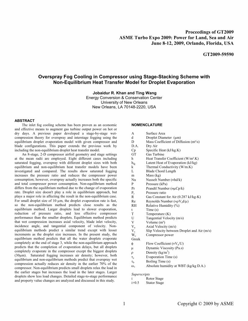
Figure 2(a) Designed compressor tip and hub diameters (the numbers on the top of the curves represent the stage numbers)

In Case 1 (design case), the axial velocity is kept as a constant in

each stage by adjusting the flow area (i.e. hub and tip diameters). The

variation of hub and tip diameters in different stages is shown in Fig.

2(a). For the cases of inlet fogging, the designed geometry is

unchanged; the local flow velocity vector, thermal properties, rotor

loading condition of each stage are calculated by the stage-stacking

scheme. An example showing the effect of fogging on the velocity

diagram is illustrated in Fig. 2(b) by juxtaposing the velocity

diagrams of Stage 2 in Cases 1, 3 and 4 for comparison between

equilibrium and non-equilibrium cases. The following differences are

observed:

a. All the velocity directions and magnitudes are changed. For

example, the absolute rotor inlet velocity changes from purely

axial direction to deviating 0.39° for Case 2, 1.89° for Case 3,

and 1.94° for Case 4 from the axis.

b. The flow coefficient (φ = Va/U) increases 2.7% for Case 2,

22.3% for Case 3 and 23.6% for Case 3.

Case 1

Case 3

Case 4

U

Va2.5

Deviation of axial velocity

for non-equilibrium

Deviation of axial velocity

for Fog Cooling Va2.5

V2.5 V2.5 Va2

Va2

V2 W2

W2.5

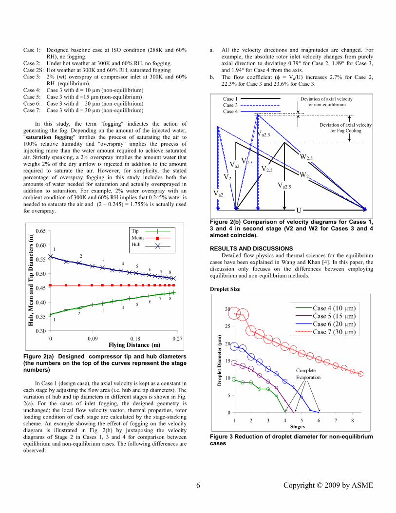
Figure 2(b) Comparison of velocity diagrams for Cases 1, 3 and 4 in second stage (V2 and W2 for Cases 3 and 4 almost coincide). RESULTS AND DISCUSSIONS

Detailed flow physics and thermal sciences for the equilibrium

cases have been explained in Wang and Khan [4]. In this paper, the

discussion only focuses on the differences between employing

equilibrium and non-equilibrium methods.

Droplet Size

0

5

10

15

20

25

30

1 2 3 4 5 6 7 8Stages

Droplet Diameter (µm)

Case 4 (10 µm)Case 5 (15 µm)

Case 6 (20 µm)

Case 7 (30 µm)

Complete

Evaporation

Figure 3 Reduction of droplet diameter for non-equilibrium cases


Figure 3 shows the droplet diameter variation in different stages.

Droplets of all the cases evaporate completely before the compressor

exit except Case 7. In general, overall evaporation of all droplets is

faster in the later stages due to an increase of droplet surface area

over volume ratio with smaller droplets and increase of temperature.

The water in Case 7 does not complete evaporation because the

residence time is short comparing to the required evaporation time.

The smallest droplet diameter found for this case is 11.2 µm (Table

A3).

Evaporation Rate

Evaporation rate depends on relative humidity, droplet size

(diameter), water vapor diffusion coefficient, heat transfer to droplet,

and surrounding temperature etc. In the equilibrium method, a

sufficient amount of water is allowed to evaporate to achieve

saturation (100% RH) at the end of each stage until all the water

evaporates as shown in Case 3 in Fig 3. Figure 4 shows the relative

humidity (evaluated at the static condition) variation along the

compressor, while Fig. 5 shows the remaining liquid water in the air.

The status and composition of wet air can be clearly seen from the

information provided by these two figures and Table A.4. For

example, in Case 3, there is sufficient water to achieve saturation

until stage 3 (the third rotor); the water completely evaporates at the

end of stage 3.5 (the third stator), so the relative humidity is 100% for

all stages up to the third rotor. After the third stage, the relative

humidity generally reduces due to increased pressure and temperature

in the later stages. For example, in the beginning of the fourth stage,

the pressure is 164 kPa and temperature is 339K, for which saturation

vapor pressure is 25.3 kPa and 0.113 kg of water per kg of air is

needed to saturate the air, but only 0.0335 kg of vapor is available

which gives a 30% relative humidity.

0

20

40

60

80

100

1 2 3 4 5 6

Stages

Relative Humidity (%

)

Case 3 (Equil)

Case 4 (10 µm)

Case 5 (15 µm)

Case 6 (20 µm)

Case 7 (30 µm)

6 - 8.5

Figure 4 Variation of relative humidity for overspray cases

When non-equilibrium method is employed with the same

conditions as Case 3, the result is shown as Case 4 in Fig 3. In Case

4, water evaporates completely at the end of stage 4, which is ½ stage

later than Case 3. This implies that the result of using equilibrium

method is very close to the non-equilibrium method for droplet size

of 10 µm. However, when the droplet sizes increase, it will take

longer for water to completely evaporate. Cases 5 and 6 show 15 µm

and 20 µm droplets completely evaporate at stages 4.5 and 5.5,

respectively. Again, droplets at 30µm do not completely evaporate at

the exit of the compressor. There is about 6% (0.001kg vs. 0.0175kg)

of the initial amount of water remains with the final droplet diameter

at around 11.2 µm. This shows that the droplet diameter does not

play any role in the equilibrium method, but significantly affect the

droplet evaporation rate in the non-equilibrium method.

0.000

0.003

0.006

0.009

0.012

0.015

0.018

1 2 3 4 5 6 7 8Stages

Liquid W

ater Fraction (mass ratio with air)

Case 3 (Equil)

Case 4 (10 µm)

Case 5 (15 µm)

Case 6 (20 µm)

Case 7 (30 µm)

Figure 5 Variation of remaining liquid water fraction (mass ratio of water over moist air) in each stage for overspray cases

0.0

0.4

0.8

1.2

1.6

2.0

2.4

2.8

3.2

3.6

1 2 3 4 5 6 7 8Stages

Tim

e (M

ili Second)

Evaporation Time for Case 4

Residence Time for Case 4







Figure 6 Residence time vs. evaporation time for non-equilibrium cases (Residence time for all four cases coincide with one another)

Evaporation of droplet is characterized by particle’s

aerodynamic residence time and the time required for evaporation as

described in the model development. When the droplets reside inside

a stage longer than the required evaporation time, all the droplets


evaporate; on the other hand, if the aerodynamic residence time is

shorter than the evaporation time, droplets become smaller and fly

into next stage. Figure 6 shows the aerodynamic residence time are

close (between 0.1-0.2 ms) for all droplet sizes at all stages; whereas

the evaporation time varies significantly with the droplet sizes,

roughly in proportional to diameter square (d2). For example, at the

first stage 30 µm droplets require 3.6 ms to evaporate versus 0.4 ms

for 10 µm droplets, which is 9-fold shorter.

Air and Droplets Temperature

275

325

375

425

475

525

575

1 2 3 4 5 6 7 8Stages

Air Static Tem

perature (K)

Case 1 (ISO) Case 2 (Hot)

Case 3 (Equil) Case 4 (10 µm)

Case 6 (20 µm) Case 7 (30 µm)

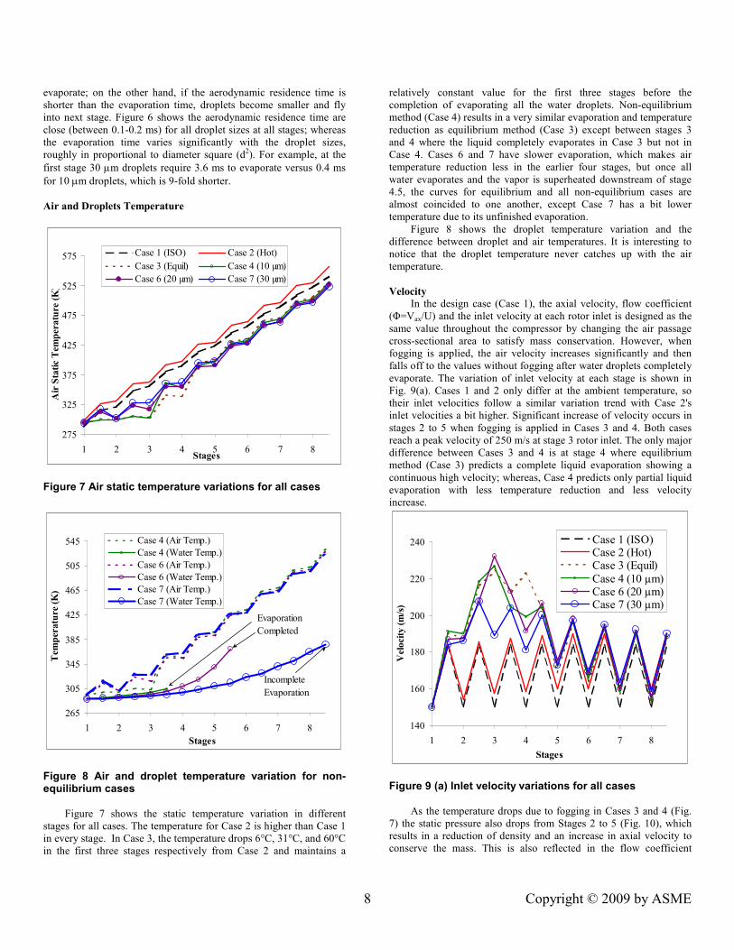
Figure 7 Air static temperature variations for all cases

265

305

345

385

425

465

505

545

1 2 3 4 5 6 7 8

Stages

Tem

perature (K)

Case 4 (Air Temp.)

Case 4 (Water Temp.)

Case 6 (Air Temp.)


Case 7 (Air Temp.)


Evaporation

Completed

Incomplete

Evaporation

Figure 8 Air and droplet temperature variation for non-equilibrium cases

Figure 7 shows the static temperature variation in different

stages for all cases. The temperature for Case 2 is higher than Case 1

in every stage. In Case 3, the temperature drops 6°C, 31°C, and 60°C

in the first three stages respectively from Case 2 and maintains a

relatively constant value for the first three stages before the

completion of evaporating all the water droplets. Non-equilibrium

method (Case 4) results in a very similar evaporation and temperature

reduction as equilibrium method (Case 3) except between stages 3

and 4 where the liquid completely evaporates in Case 3 but not in

Case 4. Cases 6 and 7 have slower evaporation, which makes air

temperature reduction less in the earlier four stages, but once all

water evaporates and the vapor is superheated downstream of stage

4.5, the curves for equilibrium and all non-equilibrium cases are

almost coincided to one another, except Case 7 has a bit lower

temperature due to its unfinished evaporation.

Figure 8 shows the droplet temperature variation and the

difference between droplet and air temperatures. It is interesting to

notice that the droplet temperature never catches up with the air

temperature.

Velocity

In the design case (Case 1), the axial velocity, flow coefficient

(Φ=Vax/U) and the inlet velocity at each rotor inlet is designed as the

same value throughout the compressor by changing the air passage

cross-sectional area to satisfy mass conservation. However, when

fogging is applied, the air velocity increases significantly and then

falls off to the values without fogging after water droplets completely

evaporate. The variation of inlet velocity at each stage is shown in

Fig. 9(a). Cases 1 and 2 only differ at the ambient temperature, so

their inlet velocities follow a similar variation trend with Case 2's

inlet velocities a bit higher. Significant increase of velocity occurs in

stages 2 to 5 when fogging is applied in Cases 3 and 4. Both cases

reach a peak velocity of 250 m/s at stage 3 rotor inlet. The only major

difference between Cases 3 and 4 is at stage 4 where equilibrium

method (Case 3) predicts a complete liquid evaporation showing a

continuous high velocity; whereas, Case 4 predicts only partial liquid

evaporation with less temperature reduction and less velocity

increase.

140

160

180

200

220

240

1 2 3 4 5 6 7 8

Stages

Velocity (m/s)

Case 1 (ISO)Case 2 (Hot)Case 3 (Equil)

Case 4 (10 µm)Case 6 (20 µm)Case 7 (30 µm)

Figure 9 (a) Inlet velocity variations for all cases

As the temperature drops due to fogging in Cases 3 and 4 (Fig.

7) the static pressure also drops from Stages 2 to 5 (Fig. 10), which

results in a reduction of density and an increase in axial velocity to

conserve the mass. This is also reflected in the flow coefficient


increase in Fig. 9b. On the other hand, due to slower evaporation of

larger droplets in Cases 6 and 7, temperature does not have any

sudden drop, so these two cases have less drastic changes in velocity

and flow coefficient. Overall speaking, all the fogging cases (Cases

3-7) have higher flow coefficients until 7th stage; afterwards their

flow coefficients drop below Case 2. This behavior is consistent with

the results obtained by White and Meacock [22], where they showed

that the flow coefficient (φ) increases till third stage and then decreased and eventually got lower than the dry compression values.

0.50

0.55

0.60

0.65

0.70

0.75

0.80

1 2 3 4 5 6 7 8

Stages

Flow C

oefficien

t (Φ

)

Case 1 (ISO)

Case 2 (Hot)

Case 3 (Equil)

Case 4 (10 µm)

Case 6 (20 µm)

Case 7 (30 µm)

Figure 9 (b) Flow coefficient variations for all cases

Combining the information obtained in Figs. 7 and 9, the results

show that the flow coefficient must significantly increase to

accommodate more mass flow rate contributed by overspray

especially when the air (not air-liquid mixture) density reduces, as

shown in Fig. 10, rather than increases after overspray is applied. The

trend of decreased air density with overspray fogging seems counter-

intuitive initially, but this phenomenon has specifically explained by

Wang and Khan [3, 4]. They explained that when overspray is

applied, temperature drops significantly (70-90oC) due to water

evaporation. This excessive temperature reduction results in a

significant reduction in pressure. Pressure usually reduces more than

the temperature as it can be seen from the polytropic relation that

PTk/(k-1) = Constant, i.e. P ∝ T(k-1)/k. Take k = 1.36 for moist air for

example, so k/(k-1) = 3.78, which means if the temperature (absolute

value) reduces 10%, the pressure will reduce 30%. Based on the ideal

gas law ρ ~ P/RT, the density reduces instead of increasing. Although the air receives more water vapor when water droplets

vaporize, the slightly increased density due to water evaporation is

not large enough to compensate for the density reduction due to

temperature-induced pressure reduction. Eventually, the air density of

oversprayed cases becomes denser than non-fogging case after stage

6.5. This density variation trend due to overspray fogging is also in

agreement with the results White and Meacock [22] and Roumeliotis

and Mathioudakis [15]. Note that the air density of saturated fogging

case (Case 2S) will always be higher than non-fogging case as have

been shown in [4] because no wet-compression and no water

evaporation occurs inside the compressor.

Pressure Ratio

The static pressure distributions are shown in Fig. 10. Saturated

fogging (Case 2S) increases static pressure as expected, while

overspray reduces the local static pressure due to continuous water

evaporation inside the compressor. Equilibrium method (Case 3)

results in lower static pressure between stages 3 and 4, but ends up

with a little higher pressure than non-equilibrium cases.

0

100

200

300

400

500

600

700

800

1 2 3 4 5 6 7 8Stages

Static Pressure (kPa)

Case 1 (ISO)

Case 2 (Hot)

Case 3 (Equil)

Case 4 (10 µm)

Case 5 (15 µm)

Case 6 (20 µm)

Case 7 (30 µm)

600

650

700

750

800

8 8.5

Figure 10 Stage static pressure variation for all cases

Figures 13a and 13b show the local and accumulative stagnation

pressure ratios. Again, Case 2S (saturated fogging) is shown to

achieve the highest overall stagnation pressure ratio (8.54), which is

noticeably above the stagnation pressure ratio from non-equilibrium

Cases 4, 5, 6 and 7 with the values of 7.63, 7.58, 7.48 and 7.33,

respectively (see Fig. 13b or Table A2).

0.40

0.60

0.80

1.00

1.20

1.40

1 2 3 4 5 6 7 8

Stages

Rotor W

ork

Coefficien

t (φ)

Case 1 (ISO)

Case 2 (Hot)

Case 3 (Equil)

Case 4 (10 µm)

Case 6 (20 µm)

Case 7 (30 µm)

Figure 11 Rotor Work Coefficient variation for all cases

For Case 2, when ambient is hot, the local stagnation pressure

ratio at the first stage drops from 1.396 of the ISO condition (Case 1)


to 1.366. At the last stage, the local stagnation pressure ratio of Case

2 is 1.206 versus 1.208 of Case 1. When fogging is applied in Case

3, the local stagnation pressure ratio experiences a significant drop

from 1.4 to 1.0 at the first stage due to reduced temperature, but the

local stagnation pressure ratios of Stags 2-4 immediately rise above

1.6, indicating the rotors of these two stages work very hard as

evidenced in their high work coefficients (ψ) shown in Fig. 11. Not until the fifth stage, does the local stagnation pressure ratio of Case 3

reduce to a level around 1.32, which is about 5% higher than Case 1.

0.5

1.5

2.5

3.5

4.5

5.5

1 2 3 4 5 6 7 8

Stages

Air D

ensity (kg/m

³)

Case 1 (ISO)

Case 2 (Hot)

Case 2S (Sat.)

Case 3 (Equil)

Case 4 (10 µm)

Case 6 (20 µm)

Case 7 (30 µm)

Figure 12 Moist Air density variation for all cases

0.9

1.0

1.1

1.2

1.3

1.4

1.5

1.6

1.7

1 2 3 4 5 6 7 8Stage

Stage Stagnation Pressure Ratio

Case 1 (ISO)

Case 2 (Hot)

Case 3 (Equil)

Case 4 (10 µm)

Case 6 (20 µm)

Case 7 (30 µm)

Figure 13(a) Stage overall stagnation pressure ratio variation for all cases

When non-equilibrium method is applied in Case 4, the local

stagnation pressure ratio is higher than those calculated by

equilibrium method in Case 3 at stages 1-3. An obvious difference

between Case 3 and 4 (or equilibrium versus non-equilibrium

approaches) is between Stage 3 and 4 where all liquid is predicted

completely evaporated in Cases 3 but not yet in Case 4. This

difference results in more cooling, lower static temperature (Fig. 7),

lower static pressure (Fig. 10), and lower density (Fig. 12) in Case 3,

but higher local stagnation pressure ratio between stages 3.5 and 5

than in Case 4. More liquid evaporated accompanied with low

overall density leads to more volume flow rate and hence higher inlet

velocity (Fig. 9a) and flow coefficient (Fig. 9b) for Case 3 between

stages 3.5 and 4.

0

1

2

3

4

5

6

7

8

1 2 3 4 5 6 7 8Stage

Cumulative Pressure Ratio

Case 1 (ISO)

Case 2 (Hot)

Case 3 (Equil)

Case 4 (10 µm)

Case 6 (20 µm)

Case 7 (30 µm)

6.50

6.75

7.00

7.25

7.50

7.75

8.00

8 8.5

Figure 13(b) Cumulative overall stagnation pressure ratio variation for all cases Compressor Power

The required compressor power (MW) is shown in Fig. 14 and

the specific work (kW/(kg/s) = kJ/kg) in P-v diagram is shown in Fig.

15. In contrast to saturated fogging which actually reduces

compressor power, overspray (Cases 3 versus Case 2) increases both

specific compressor work by 8.65% due to increased pressure ratio

and the total compressor power by 12.6% due to increased mass flow

rate. This seemingly counter-intuition phenomenon was explained in

detail in the previous paper [4] and is not repeated here. Basically,

overspray increases stagnation pressure ratio and the compressor

work increases, which can be represented by the area on the left of

the compression curve on the P-v diagram. The specific work for Case 3 (272 kJ/kg) is very close to Case 4

(271 kJ/kg). The total powers for both cases are also very close

(7.909 MW vs. 7.873 MW) because their mass flow rates are

identical (26.71 kg/s) as shown in Table 1. As the diameter increases

from 10 µm to 30 µm, the specific work decreases from 271 to 263

kJ/kg. Since less power is used to produce less pressure ratio, a fair

way to compare the compressor performance is to compare the

compressor power per unit increase of pressure ratio (Wc/Pr) in Table

1. As it can be seen, equilibrium method (Case 3) predicts more

efficient compression with Wc/Pr = 1028 kW than non-equilibrium

Case 4 with Wc/Pr = 1031 kW by assuming instantaneous water

evaporation. Case 2S, having achieved Wc/Pr = 830 kW, is the most

effective in all cases due to its complete evaporation before

compression. This fact is revealed in Fig. 15, which shows the P-v

curve of Case 2s is situated at the leftmost of all the curves and

requires the least amount of specific work (248 kJ/kg) among all

cases, although it produces the highest stagnation pressure ratio

(8.54). Among the four non-equilibrium cases, Case 4 with 10 µm

(smallest droplet) is most effective among the 4 non-equilibrium

cases and Case 7 (30 µm droplet) is the least effective.

µ µ µ


0

1

2

3

4

5

6

7

8

1 2 3 4 5 6 7 8

Stage

Cumulative Power (MW)

Case 1 (ISO)

Case 2 (Hot)

Case 3 (Equil)

Case 4 (10 µm)

Case 7 (30 µm)

Case 6 (20 µm)

6.0

6.5

7.0

7.5

8.0

7 8

Figure 14 Cumulative total compressor power variation for all cases

0.0

0.2

0.4

0.6

0.8

1.0

0 0.15 0.3 0.45 0.6 0.75 0.9Specific Volume (m³/kg)

Static Pressure (MPa)

Case 2 (Hot)Case 2S (Sat.)Case 3 (Equil.)Case 4 (Non-Eq)

0.5

0.6

0.7

0.8

0.2 0.25

0.2

0.3

0.3

0.4 0.45 0.5

Figure 15 P-v diagram to show specific work for four cases

The present result of increased compressor power consumption

due to wet compression is consistent with Bagnoli et. al. [23],

Roumeliotis and Mathioudakis [24], Williams [25] and Wang and

Khan [3, 4], but inconsistent with Abdelwahab [11] and Sanaye et. al.

[12]. Although White and Meacock [22] showed compressor power

reduced with fogging, their presentation could be misleading without

looking into their assumption and practice. Their analysis indeed

showed that the compression with fogging produces more pressure

ratio than the dry compression. However, when the comparison was

made, they didn't compare the actual compressor power

consumptions corresponding to the different pressure ratios of each

case, rather they jacked up the pressure ratio of the dry compression

to equal the wet compression pressure ratio, which of course led to

the conclusion that wet compression required less power.

Table 1 Overall compressor performance and net gas turbine

output power

Cases Mass

flow rate

(kg/s)

Specific

Work

(kJ/kg)

Comp.

Power

(MW)

Pr Comp.

Power /Pr

(kW)

Net GT

Output

(MW)

1 26.91 244 7.139 7.42 962 8.609

2 25.77 251 7.024 7.20 975 7.904

2S 26.25 248 7.088 8.54 830 8.357

3 26.71 272 7.909 7.69 1028 9.039

4 26.71 271 7.873 7.63 1031 9.057

5 26.71 270 7.838 7.57 1035 8.971

6 26.71 268 7.780 7.48 1040 8.912

7 26.71 263 7.647 7.34 1042 8.912

It is encouraging to know that the present results are supported

by the recent experimental results from Roumeliotis and

Mathioudakis [24]. They showed that the compressor power

increased by water injection and the increased compressor power was

linear with the quantity of water entering the stage. As a result, the

compressor isentropic efficiency decreases linearly with the amount

of water injected.

Although the compressor power consumption increases in the

saturated fogging and overspray cases, the total gas turbine net power

increases nonetheless as shown in Table 1.

SUMMARY

This paper compares the results of thermal equilibrium and non-

equilibrium methods for overspray fogging through stag-stacking

scheme with given mean-line blade and 8-stage compressor

configurations. The results are summarized below:

1. Saturated fogging achieves highest pressure ratio augmentation

and reduces compressor power consumption; whereas overspray

actually increases both the specific and overall compressor

power for both equilibrium and non-equilibrium cases.

Nevertheless, the net GT power output increases with both

saturated and overspray fogging.

2. Non-equilibrium method differs from the equilibrium method

due to the change of evaporation rate. Droplet size doesn't play a

role in equilibrium approach, but plays a major role in affecting

the result in the non-equilibrium case. For small droplet size of

10 µm, the droplet evaporation rate is fast, so the non-

equilibrium method predicts close results as the equilibrium

method. Larger droplets lead to slower evaporation, reduction

of pressure ratio, and less effective compressor performance

than the smaller droplets.

3. Equilibrium method predicts that wet compression increases

axial velocity, blade inlet velocity, incidence angle, and

tangential component of velocity. Non-equilibrium methods

predict a similar trend except with lesser increments as the

droplet size increases.

4. In the present study, the equilibrium method predicts that all the

water droplets evaporate completely at the end of stage 3, while

the non-equilibrium approach predicts that the completion of

evaporation delays; but all droplets completely evaporate in the

µ

µ

µ


compressor except approximately 10% of the biggest droplets

(30µm) escape from the compressor.

5. Saturated fogging increases air density; however, both

equilibrium and non-equilibrium methods predict that wet

compression actually reduces air density in the earlier 70% of

the compressor.

6. Non-equilibrium predicts small droplets relax the load in the

earlier stages, but increases the load in the later stages. Larger

droplets show less load changes.

ACKNOWLEDGEMENT

This study was supported by the Louisiana Governor's Energy

Initiative via the Clean Power and Energy Research Consortium

(CPERC) and administered by the Louisiana Board of Regents.

REFERENCES

1. Meher-Homji, C.B. and Mee, T.R., 1999, "Gas Turbine Power

Augmentation by Fogging of Inlet Air," Proceedings of 28th

Turbomachinery Symposium, Houston, Texas, USA, September

1999.

2. Bagnoli, M., Bianchi, M., Melino, F., Peretto, A., Spina, P.R.,

Bhargava, R. and Ingistov, S., 2004, "A Parametric Study of

Interstage Injection on GE Frame 7EA Gas Turbine,"

Proceedings of ASME Turbo Expo 2004, Vienna, Austria, June

14-17, ASME Paper No: GT-2004-53042.

3. Wang, T. and Khan, J. R., 2008, "Overspray and Interstage Fog

Cooling in Compressor using Stage-Stacking Scheme -- Part 1:

Development of Theory and Algorithm", Proceedings of ASME

Turbo Expo 2008, Berlin, Germany, June 9-13, 2008, ASME

Paper No: GT-2008-50322.

4. Wang, T. and Khan, J. R., 2008, "Overspray and Interstage Fog

Cooling in Compressor using Stage-Stacking Scheme -- Part 2:

Case Study," Proceedings of ASME Turbo Expo 2008, Berlin,

Germany, June 9-13, 2008, ASME Paper No: GT-2008-50323.

5. Hill P. G., "Aerodynamic and Thermodynamic Effects of

Coolant Injection on Axial Compressors," Aeronautical

Quarterly, February 1963, pp. 333-348.

6. Zheng, Q., Sun, Y., Li, S. and Wang, Y, 2002, "Thermodynamic

Analysis of Wet Compression Process in the Compressor of Gas

Turbine," Proc. of ASME Turbo Expo 2002, Amsterdam, The

Netherlands, June 3-6, ASME Paper No: GT-2002-30590.

7. Zheng, Q., Li, M., Sun, Y., 2003, "Thermodynamic Analysis of

Wet Compression and Regenerative (WCR) Gas Turbine,"

Proceedings of ASME Turbo Expo 2003, Atlanta, Georgia,

USA, June 16-19, ASME Paper No: GT-2003-38517.

8. Khan, J. R. and Wang, T., 2006, "Fog and Overspray Cooling

for Gas Turbine Systems with Low Calorific Value Fuels,"

Proceedings of ASME Turbo Expo 2006, Barcelona, Spain, May

8-11, 2006, ASME Paper No: GT-2006-90396.

9. Williams, J., "Further Effects of Water Ingestion on Axial Flow

Compressors and Aeroengines at Part Speed," Proceedings of

ASME Turbo Expo 2008, Berlin, Germany, June 9-13, 2008,

ASME Paper No: GT2008-50620.

10. Payne, R.C. and White, A.J., 2007, "Three-Dimensional

Calculations of Evaporative Flow in Compressor Blade Rows,"

Proceedings of ASME Turbo Expo 2007, Montreal, Canada,

May 14-17, 2007, ASME Paper No: GT-2007-27331.

11. Abdelwahab, A., 2006, "An Investigation Of The Use Of Wet

Compression In Industrial Centrifugal Compressors,"

Proceedings of ASME Turbo Expo 2006, Barcelona, Spain, May

8-11, 2006, ASME Paper No: GT-2006-90695.

12. Sanaye, S., Rezazadeh, H., and Aghazeynali, M., 2006, "Effects

of Inlet Fogging and Wet Compression on Gas Turbine

Performance," Proceedings of ASME Turbo Expo 2006,

Barcelona, Spain, May 8-11, 2006, ASME Paper No: GT-2006-

90719.

13. Bianchi, M., Melino, F., Peretto, A., Spina, P.R. and Ingistov S.,

2007, "Influence of Water Droplet Size and Temperature on Wet

Compression," Proceedings of ASME Turbo Expo 2007,

Montreal, Canada, May 14-17, 2007, ASME Paper No: GT-

2007-27458.

14. Sexton, M. R., Urbach, H. B., Knauss, D. T., 1998 "Evaporative

Cooling for NOx Suppression and Enhanced Engine

Performance for Naval Gas Turbine Propulsion Plants," ASME

paper 98-GT-332.

15. Roumeliotis I., Mathioudakis K., 2006, "Evaluation of Interstage

Water Injection Effect on Compressor and Engine

Performance," ASME Journal of Engineering for Gas Turbine

and Power, Paper GTP-05-1123, Vol. 128/4, pp. 849-856, also

ASME paper 2005-GT-68698.

16. Khan, J. R. and Wang, T., 2008, "Simulation of Inlet Fogging

and Wet-compression in a Single Stage Compressor Including

Erosion Analysis," Proceedings of ASME Turbo Expo 2008,

Berlin, Germany, June 9-13, 2008, ASME Paper No: GT-2008-

50874.

17. Chai, Y. 1995, "Two-Phase Flows in Steam Turbine," Xi’an

Jiaotong University Press.

18. Kuo, K. K. Y., "Principles of Combustion," John Wiley and

Sons, New York, 1986.

19. Handbook Of Chemistry, CRC Press, 59th Edition.

20. Young J. B., "The Fundamental Equations of Gas-Droplet

Multiphase Flow," Int. J. Multiphase Flow, Vol. 21, No. 2,

pp.175-191, 1995.

21. Klepper J., Hale A., Davis M., Hurwitz W., "A Numerical

Investigation of the Effects of Steam Ingestion on Compression

System Performance," ASME paper No. GT2004-54190.

22. White A. J., Meacock A J., 2004, "An evaluation of the effects

of water injection on compressor performance," ASME J. of

Engineering for Gas Turbines and Power, Vol. 126, pp.748-754.

23. Bagnoli, M., Bianchi, M., Melino, F. and Spina, P.R., 2006,

"Development and Validation of a Computational Code for Wet

Compression Simulation of Gas Turbines," Proceedings of

ASME Turbo Expo 2006, Barcelona, Spain, May 8-11, 2006,

ASME Paper No: GT-2006-90342.

24. Roumeliotis, I. and Mathioudakis, K., 2007, "Water Injection

Effects on Compressor Stage Operation," ASME Journal of

Engineering for Gas Turbines and Power, Vol. 129, pp. 778-784.

25. Williams, J., 2008, "Further Effects of Water Ingestion on Axial

Flow Compressors and Aeroengines at Part Speed", Proceedings

of ASME Turbo Expo 2008, Berlin, Germany, June 9-13,

ASME Paper No: GT-2008-50620.


APPENDIX Table A1 Detailed stage-stacking data (pressures, temperature, velocity, flow coefficient, Mach numbers and density) for all cases. (Shaded areas represent the stator stages and the non-shaded rows represent rotor stages.) Table A2 Detailed stage-stacking data (pressure ratio, power, rotor work coefficient, de Haller number) for all cases

Case 1 Case 2 Case 3 Case 4 Case 5 Case 6 Case 7 Case 1 Case 2 Case 3 Case 4 Case 5 Case 6 Case 7

1 1.396 1.366 1.000 1.085 1.231 1.308 1.364 1 892.4 833.0 634.5 617.1 725.8 811.6 865.3

2 1.355 1.344 1.112 1.146 1.181 1.164 1.164 2 892.4 864.6 725.5 725.8 885.1 897.5 918.2

3 1.318 1.319 1.651 1.652 1.444 1.365 1.356 3 892.4 889.8 1346.0 1562.8 1360.1 1155.1 1032.2

4 1.288 1.287 1.593 1.395 1.341 1.333 1.333 4 892.4 886.2 1435.8 1165.3 1038.3 1041.2 1011.4

5 1.263 1.262 1.311 1.321 1.327 1.316 1.292 5 892.4 888.3 942.3 962.5 975.3 995.2 961.6

6 1.241 1.242 1.291 1.295 1.298 1.305 1.278 6 892.4 889.9 966.7 973.7 979.3 991.7 974.3

7 1.223 1.222 1.258 1.260 1.263 1.267 1.254 7 892.4 886.1 934.7 939.9 944.8 953.0 949.2

8 1.208 1.206 1.234 1.236 1.238 1.241 1.234 8 892.4 885.8 923.2 925.9 929.0 934.6 935.1Overall 7.436 7.199 7.684 7.634 7.582 7.481 7.333 Overall 7139 7024 7909 7873 7838 7780 7647

Stage


1 0.737 0.718 0.528 0.513 0.604 0.675 0.720 1 0.726 0.737 0.846 0.855 0.803 0.762 0.736

2 0.737 0.746 0.604 0.604 0.736 0.747 0.764 2 0.726 0.727 0.851 0.854 0.773 0.755 0.736

3 0.737 0.767 1.120 1.300 1.132 0.961 0.859 3 0.726 0.716 0.666 0.592 0.615 0.668 0.696

4 0.737 0.764 1.195 0.969 0.864 0.866 0.841 4 0.726 0.716 0.586 0.652 0.688 0.691 0.695

5 0.737 0.766 0.784 0.801 0.811 0.828 0.800 5 0.726 0.715 0.709 0.705 0.702 0.700 0.707

6 0.737 0.767 0.804 0.810 0.815 0.825 0.811 6 0.726 0.713 0.694 0.693 0.693 0.692 0.698

7 0.737 0.764 0.778 0.782 0.786 0.793 0.790 7 0.726 0.715 0.699 0.699 0.699 0.698 0.701

8 0.737 0.764 0.768 0.770 0.773 0.778 0.778 8 0.726 0.715 0.699 0.699 0.699 0.699 0.702

StageStage Power (KW)

StageRotor Work Coefficient de Haller Number

StageStage Pressure Ratio

Table A3 Non-equilibrium data (Droplet temperature, diameter, evaporation/boiling time, residence time) for all cases

Case 4 Case 5 Case 6 Case 7 Case 4 Case 5 Case 6 Case 7 Case 4 Case 5 Case 6 Case 7 Case 4 Case 5 Case 6 Case 7

1 288.0 288.0 288.0 288.0 1 9.573 14.359 19.145 28.718 1 0.3900 0.8775 1.5600 3.5852 1 0.1048 0.1048 0.1048 0.1048

1.5 289.9 289.5 289.2 288.7 1.5 8.666 13.475 18.491 28.295 1.5 0.1753 0.3766 0.6440 1.4101 1.5 0.1460 0.1493 0.1511 0.1519

2 292.7 291.8 291.1 289.8 2 8.647 12.482 16.105 23.684 2 0.1475 0.2798 0.4349 0.8602 2 0.0705 0.0731 0.0755 0.0771

2.5 294.5 293.8 292.7 290.8 2.5 6.828 10.727 14.641 22.598 2.5 0.1112 0.2423 0.4107 0.9277 2.5 0.1027 0.1080 0.1080 0.1080

3 297.7 297.3 295.9 292.9 3 6.828 8.841 12.569 21.243 3 0.0940 0.1497 0.2712 0.6985 3 0.0478 0.0521 0.0559 0.0593

3.5 304.1 302.2 299.6 295.0 3.5 4.790 7.139 11.200 20.321 3.5 0.0559 0.1116 0.2441 0.7715 3.5 0.0897 0.0860 0.0870 0.0898

4 351.0 319.0 308.6 299.0 4 0.000 3.415 8.986 19.101 4 0.0000 0.0278 0.1457 0.5778 4 0.0467 0.0488 0.0484 0.0495

4.5 392.4 389.7 318.4 302.6 4.5 0.000 7.345 18.264 4.5 0.0000 0.1142 0.6375 4.5 0.0747 0.0740 0.0742 0.0764

5 398.3 395.5 339.5 308.8 5 4.349 17.135 5 0.0426 0.4739 5 0.0426 0.0422 0.0415 0.0423

5.5 428.6 426.5 369.3 314.1 5.5 0.678 16.352 5.5 0.0019 0.5207 5.5 0.0656 0.0652 0.0644 0.0656

6 433.9 431.8 428.2 322.5 6 0.000 15.288 6 0.0000 0.3837 6 0.0365 0.0363 0.0359 0.0361

6.5 463.9 462.2 459.4 329.6 6.5 14.551 6.5 0.4208 6.5 0.0573 0.0570 0.0566 0.0568

7 469.5 467.8 464.9 340.8 7 13.534 7 0.3106 7 0.0321 0.0319 0.0316 0.0316

7.5 497.7 496.2 493.8 350.2 7.5 12.828 7.5 0.3411 7.5 0.0504 0.0502 0.0499 0.0498

8 503.5 501.9 499.4 364.7 8 11.854 8 0.2580 8 0.0282 0.0281 0.0279 0.0278

8.5 530.5 529.2 527.1 376.6 8.5 11.198 8.5 0.2910 8.5 0.0445 0.0444 0.0442 0.0440

Evap./ Boil. Time (ms)Stage

Residence Time (ms)StageStage

Droplet Temp. (K)Stage

Droplet Dia. (µm)


1 115.6 115.1 115.7 115.7 115.7 115.7 115.7 1 101.3 101.3 101.3 101.3 101.3 101.3 101.3

1.5 161.6 157.4 115.7 125.6 142.5 151.6 158.0 1.5 134.9 132.2 108.5 107.2 117.0 125.6 131.5

2 161.4 157.2 115.7 125.6 142.4 151.4 157.8 2 144.7 139.3 108.7 107.3 107.7 108.4 108.7

2.5 218.9 211.5 128.7 143.9 168.3 176.3 183.9 2.5 185.8 180.0 115.7 113.9 132.9 139.9 146.2

3 218.6 211.2 128.6 143.8 168.1 176.2 183.7 3 201.9 188.4 113.3 111.3 114.4 129.0 146.7

3.5 288.5 279.0 212.9 250.6 243.1 240.9 249.5 3.5 248.4 240.1 167.9 205.3 193.9 193.1 203.6

4 288.1 278.6 212.5 250.0 242.8 240.5 249.2 4 271.4 250.7 164.1 191.5 193.9 193.0 207.9

4.5 371.4 358.9 339.1 330.2 325.8 321.1 332.6 4.5 323.8 312.2 281.4 272.1 267.9 264.1 277.8

5 371.0 358.5 338.5 329.8 325.4 320.7 332.2 5 354.3 325.0 298.5 288.3 283.1 272.2 286.6

5.5 468.9 453.0 444.5 436.1 432.4 422.4 429.7 5.5 413.1 397.8 379.9 371.2 367.5 357.2 366.3

6 468.4 452.5 443.9 435.5 431.9 421.9 429.2 6 451.7 413.1 398.2 388.9 384.9 373.8 378.2

6.5 582.0 562.5 574.0 565.1 561.3 551.1 549.4 6.5 517.3 498.2 499.3 490.4 486.6 476.2 475.6

7 581.4 561.9 573.3 564.5 560.7 550.4 548.8 7 564.6 516.2 522.6 513.2 509.2 498.3 493.2

7.5 711.6 687.5 721.8 712.7 708.8 698.1 688.7 7.5 637.7 613.7 636.2 627.2 623.4 612.8 604.1

8 710.9 686.9 721.1 712.0 708.0 697.3 688.0 8 694.1 634.3 664.9 655.1 650.9 639.5 627.0

8.5 859.2 829.1 891.0 881.3 877.2 866.1 850.1 8.5 775.4 745.8 794.2 784.4 780.3 769.2 753.8


1 150.0 150.0 150.0 150.0 150.0 150.0 150.0 1 0.440 0.431 0.439 0.439 0.439 0.439 0.439

1.5 183.7 184.0 190.6 191.4 187.2 184.9 183.9 1.5 0.515 0.507 0.551 0.553 0.535 0.523 0.518

2 150.0 154.1 187.5 190.1 187.7 185.9 186.1 2 0.417 0.421 0.541 0.549 0.541 0.535 0.534

2.5 183.7 185.6 216.0 218.2 207.4 207.4 207.5 2.5 0.491 0.487 0.615 0.622 0.579 0.575 0.572

3 150.0 157.6 223.9 226.8 232.3 209.6 189.2 3 0.396 0.411 0.639 0.713 0.660 0.586 0.520

3.5 183.7 187.6 213.3 204.4 213.0 210.8 204.0 3.5 0.469 0.471 0.573 0.527 0.561 0.556 0.535

4 150.0 158.6 222.7 199.2 191.6 192.1 181.0 4 0.378 0.396 0.6 0.510 0.504 0.506 0.473

4.5 183.7 188.9 203.4 204.5 206.7 206.1 200.2 4.5 0.450 0.455 0.507 0.516 0.519 0.519 0.502

5 150.0 159.7 168.7 172.1 175.3 180.3 172.9 5 0.363 0.382 0.417 0.430 0.437 0.452 0.431

5.5 183.7 189.8 195.7 196.9 198.4 200.6 197.1 5.5 0.433 0.440 0.466 0.472 0.474 0.482 0.473

6 150.0 160.1 163.9 165.9 167.9 171.4 169.4 6 0.349 0.369 0.387 0.395 0.399 0.409 0.404

6.5 183.7 190.3 192.2 193.0 194.0 195.5 194.8 6.5 0.418 0.426 0.44 0.444 0.446 0.451 0.450

7 150.0 160.0 157.2 158.6 160.0 162.5 163.3 7 0.337 0.357 0.358 0.363 0.366 0.373 0.375

7.5 183.7 190.4 189.5 190.1 190.7 191.7 192.3 7.5 0.405 0.413 0.419 0.422 0.423 0.426 0.429

8 150.0 160.1 152.9 154.0 155.1 157.0 158.9 8 0.327 0.346 0.336 0.340 0.342 0.347 0.353

8.5 183.7 190.5 187.5 188.0 188.5 189.4 190.3 8.5 0.393 0.401 0.402 0.404 0.405 0.408 0.411

StageStatic Pressure (kPa)

StageAbsolute Mach Number

StageInlet Velocity (m/s)

StageTotal Pressure (kPa)


1 288.0 300.0 294.2 294.2 294.2 294.2 294.2 1 1.222 1.170 1.213 1.213 1.213 1.213 1.213

1.5 315.2 326.3 299.5 299.2 307.1 313.3 317.5 1.5 1.488 1.405 1.268 1.255 1.337 1.409 1.458

2 321.5 331.2 299.7 299.3 300.4 301.4 301.9 2 1.564 1.458 1.269 1.256 1.253 1.255 1.256

2.5 348.0 358.9 305.4 305.0 318.8 323.5 327.7 2.5 1.856 1.738 1.314 1.296 1.448 1.503 1.553

3 356.4 363.6 303.8 303.2 306.4 316.7 328.0 3 1.969 1.795 1.294 1.275 1.292 1.411 1.554

3.5 380.7 392.4 341.0 361.0 355.4 354.9 360.2 3.5 2.268 2.120 1.694 1.879 1.883 1.881 1.961

4 390.4 397.3 339.0 354.4 355.4 354.9 362.2 4 2.416 2.187 1.666 1.818 1.879 1.876 1.989

4.5 413.2 425.7 395.2 391.5 389.7 388.1 393.7 4.5 2.719 2.535 2.450 2.406 2.365 2.344 2.442

5 424.0 430.6 401.4 397.5 395.5 391.3 397.0 5 2.899 2.608 2.559 2.508 2.463 2.395 2.497

5.5 445.6 458.9 430.6 427.8 426.6 423.1 426.1 5.5 3.216 2.993 3.009 2.974 2.939 2.881 2.948

6 457.1 463.9 436.0 433.1 431.8 428.2 429.7 6 3.428 3.075 3.115 3.077 3.040 2.978 3.014

6.5 477.8 492.0 465.6 463.3 462.2 459.4 459.2 6.5 3.759 3.501 3.669 3.634 3.599 3.542 3.551

7 489.9 497.0 471.3 468.8 467.8 465.0 463.7 7 4.001 3.591 3.793 3.758 3.724 3.667 3.648

7.5 509.8 524.8 499.1 497.1 496.2 493.8 491.8 7.5 4.342 4.041 4.357 4.326 4.295 4.244 4.211

8 522.3 529.8 505.0 502.9 501.9 499.4 496.7 8 4.613 4.137 4.500 4.466 4.432 4.377 4.324

8.5 541.6 557.5 531.9 530.0 529.2 527.1 524.0 8.5 4.970 4.623 5.108 5.074 5.042 4.990 4.924


1 0.953 0.932 0.949 0.949 0.949 0.949 0.949 1 0.521 0.521 0.521 0.521 0.521 0.521 0.521

1.5 0.661 0.659 0.793 0.802 0.744 0.700 0.672 1.5 0.521 0.529 0.607 0.613 0.576 0.547 0.528

2 0.902 0.899 1.078 1.089 1.048 1.012 0.991 2 0.521 0.535 0.637 0.644 0.646 0.644 0.644

2.5 0.629 0.628 0.905 0.918 0.784 0.736 0.699 2.5 0.521 0.533 0.731 0.741 0.663 0.639 0.618

3 0.857 0.862 1.245 1.264 1.150 1.056 0.979 3 0.521 0.547 0.787 0.799 0.789 0.722 0.655

3.5 0.602 0.595 0.78 0.655 0.655 0.665 0.650 3.5 0.521 0.534 0.692 0.624 0.623 0.624 0.598

4 0.818 0.822 1.087 0.940 0.928 0.938 0.908 4 0.521 0.551 0.750 0.687 0.665 0.666 0.628

4.5 0.577 0.568 0.59 0.602 0.609 0.620 0.605 4.5 0.521 0.536 0.574 0.585 0.595 0.600 0.576

5 0.785 0.787 0.823 0.838 0.848 0.866 0.845 5 0.521 0.555 0.586 0.598 0.609 0.626 0.601

5.5 0.556 0.545 0.56 0.567 0.571 0.580 0.574 5.5 0.521 0.536 0.553 0.559 0.566 0.578 0.565

6 0.756 0.757 0.781 0.790 0.794 0.806 0.801 6 0.521 0.556 0.569 0.576 0.583 0.596 0.588

6.5 0.537 0.525 0.525 0.530 0.533 0.539 0.541 6.5 0.521 0.536 0.530 0.535 0.540 0.549 0.548

7 0.730 0.731 0.735 0.741 0.744 0.753 0.756 7 0.521 0.556 0.546 0.551 0.556 0.564 0.567

7.5 0.520 0.508 0.499 0.503 0.505 0.510 0.515 7.5 0.521 0.536 0.516 0.519 0.523 0.529 0.534

8 0.707 0.708 0.7 0.705 0.707 0.713 0.720 8 0.521 0.556 0.530 0.534 0.538 0.545 0.552

8.5 0.504 0.493 0.477 0.480 0.482 0.486 0.492 8.5 0.521 0.537 0.503 0.507 0.510 0.515 0.522

Flow Coefficient (Φ)

StageStatic Temperature (K)

StageDensity (kg/m

3)

Relative Mach NumberStageStage

(µµµµm)


Table A4 Liquid and phase data for fogging cases

Case 3 Case 4 Case 5 Case 6 Case 7 Case 3 Case 4 Case 5 Case 6 Case 7

1 0.01754 0.01754 0.01754 0.01754 0.01754 1 0.01596 0.01596 0.01596 0.01596 0.01596

1.5 0.01282 0.01301 0.01450 0.01581 0.01678 1.5 0.02069 0.02049 0.01901 0.01770 0.01673

2 0.01264 0.01293 0.01152 0.01044 0.00984 2 0.02087 0.02058 0.02199 0.02307 0.02367

2.5 0.00610 0.00637 0.00731 0.00785 0.00855 2.5 0.02741 0.02714 0.02619 0.02566 0.02496

3 0.00610 0.00637 0.00410 0.00496 0.00710 3 0.02741 0.02714 0.02941 0.02854 0.02641

3.5 0 0.00220 0.00216 0.00351 0.00622 3.5 0.03351 0.03131 0.03135 0.03000 0.02729

4 0 0 0.00024 0.00181 0.00516 4 0.03351 0.03351 0.03327 0.03170 0.02835

4.5 0 0 0 0.00099 0.00451 4.5 0.03351 0.03351 0.03351 0.03252 0.02900

5 0 0 0 0.00021 0.00373 5 0.03351 0.03351 0.03351 0.03330 0.02978

5.5 0 0 0 0 0.00324 5.5 0.03351 0.03351 0.03351 0.03351 0.03027

6 0 0 0 0 0.00265 6 0.03351 0.03351 0.03351 0.03351 0.03086

6.5 0 0 0 0 0.00228 6.5 0.03351 0.03351 0.03351 0.03351 0.03123

7 0 0 0 0 0.00184 7 0.03351 0.03351 0.03351 0.03351 0.03167

7.5 0 0 0 0 0.00156 7.5 0.03351 0.03351 0.03351 0.03351 0.03195

8 0 0 0 0 0.00123 8 0.03351 0.03351 0.03351 0.03351 0.03227

8.5 0 0 0 0 0.00104 8.5 0.03351 0.03351 0.03351 0.03351 0.03247

StageLiquid Water Fraction

StageWater Vapor Fraction

Table A5 Rotor-stator camber line geometries and stage information. Incidence angle i is for the i-th rotor stage and deviation

angle δδδδ is for the flow leaving i+0.5th stator.

1 0.636 0.560 0.356 3.400 -62.47 0.00 0.00 0.00 0.00 0.00 0.00 0.00 0.00 0.00 0.00 0.00 0.00 0.00 0.00 0.00

1.5 0.691 0.542 0.374 2.794 -50.47 35.25 0.00 0.00 0.00 -1.07 0.00 -11.76 0.00 -12.54 0.00 -7.59 0.00 -3.55 0.00 -0.97

2 0.703 0.538 0.378 2.658 -62.47 0.00 0.00 0.00 0.39 -1.07 1.89 -11.76 1.94 -12.54 3.22 -7.59 4.26 -3.55 4.98 -0.97

2.5 0.744 0.525 0.391 2.240 -50.47 35.25 0.00 0.00 0.39 -1.01 1.89 -22.01 1.94 -22.91 3.22 -12.14 4.26 -7.68 4.98 -4.28

3 0.757 0.521 0.395 2.111 -62.47 0.00 0.00 0.00 0.93 -1.01 3.76 -22.01 3.83 -22.91 6.54 -12.14 5.82 -7.68 4.47 -4.28

3.5 0.786 0.513 0.403 1.833 -50.47 35.25 0.00 0.00 0.93 -0.24 3.76 -14.31 3.83 -6.74 6.54 -2.55 5.82 -3.63 4.47 -2.80

4 0.797 0.510 0.406 1.721 -62.47 0.00 0.00 0.00 1.28 -0.24 4.79 -14.31 4.92 -6.74 5.34 -2.54 5.05 -3.63 3.84 -2.80

4.5 0.818 0.504 0.412 1.529 -50.47 35.25 0.00 0.00 1.28 0.10 4.79 0.40 4.92 -0.60 5.34 -1.17 5.05 -2.17 3.84 -1.15

5 0.828 0.501 0.415 1.434 -62.47 0.00 0.00 0.00 1.51 0.10 2.94 0.40 3.19 -0.60 3.49 -1.17 3.92 -2.17 3.16 -1.15

5.5 0.844 0.497 0.419 1.292 -50.47 35.25 0.00 0.00 1.51 0.34 2.94 0.37 3.19 -0.08 3.49 -0.47 3.92 -1.20 3.16 -0.75

6 0.853 0.494 0.422 1.212 -62.47 0.00 0.00 0.00 1.64 0.34 2.22 0.37 2.41 -0.08 2.61 -0.46 2.94 -1.20 2.75 -0.75

6.5 0.865 0.491 0.425 1.106 -50.47 35.25 0.00 0.00 1.64 0.58 2.22 2.18 2.41 1.81 2.61 1.44 2.94 0.83 2.75 0.73

7 0.873 0.489 0.427 1.039 -62.47 0.00 0.00 0.00 1.69 0.58 1.60 2.18 1.74 1.81 1.88 1.44 2.11 0.83 2.21 0.73

7.5 0.882 0.487 0.429 0.957 -50.47 35.25 0.00 0.00 1.69 0.61 1.60 3.21 1.74 2.94 1.88 2.64 2.11 2.14 2.21 1.75

8 0.889 0.485 0.431 0.901 -62.47 0.00 0.00 0.00 1.70 0.61 1.13 3.22 1.25 2.94 1.37 2.64 1.56 2.14 1.77 1.76

8.5 0.896 0.483 0.433 0.836 -50.47 35.25 0.00 0.00 1.70 0.60 1.13 4.16 1.25 3.90 1.37 3.63 1.56 3.20 1.77 2.61

Case 7

i1 / δ1i1.5 /

δ1.5

Chord

Length

(cm)

i1.5 /

δ1.5i1 / δ1

ß1' /

ß1.5'

α1' /

α1.5'

Case 1 Case 3

Stage

Hub to

Tip

Ratio

Tip

Dia.

(m)

Hub

Dia.

(m)i1 / δ1

i1.5 /

δ1.5i1 / δ1

i1.5 /

δ1.5

i1.5 /

δ1.5i1 / δ1

i1.5 /

δ1.5

Case 2

i1 / δ1i1.5 /

δ1.5

Case 4 Case 5 Case 6

i1 / δ1

W1

W1.5

β1 β '1

i1

β1.5

δ1 β '1.5

θ1

V1

V1.5

α1 α '1

i1.5

α1.5 θ1.5

α '1.5 δ1.5

Rotor

Stator i1 = |β1| – |β1'|

δ1 = |β1.5| – |β1.5'|

θ1 = β1.5' – β1'

β1 < 0, β1' < 0

β1.5 < 0, β1.5' < 0

i1.5 = |α1| – |α1'|

δ1.5 = |α1.5| – |α1.5'|

θ1.5 = α1.5' – α1'

α1 < 0, α1' < 0

α1.5 < 0, α1.5' < 0

In every stages, θ1 = 12° and θ1.5 = 35.25°

proceedings of gt2009 asme turbo expo 2009: power for …

Documents