Procedure for Calculating Estimated Ultimate Recoveries of Bakken and Three Forks Formations Horizontal Wells in the Williston Basin

By Troy A. Cook

Open-File Report 2013–1109

U.S. Department of the Interior U.S. Geological Survey

U.S. Department of the Interior SALLY JEWELL, Secretary

U.S. Geological Survey Suzette M. Kimball, Acting Director

U.S. Geological Survey, Reston, Virginia: 2013

For more information on the USGS—the Federal source for science about the Earth, its natural and living resources, natural hazards, and the environment—visit http://www.usgs.gov or call 1–888–ASK–USGS

For an overview of USGS information products, including maps, imagery, and publications, visit http://www.usgs.gov/pubprod

To order this and other USGS information products, visit http://store.usgs.gov

Suggested citation: Cook, T.A., 2013, Procedure for calculating estimated ultimate recoveries of Bakken and Three Forks Formations horizontal wells in the Williston Basin: U.S. Geological Survey Open-File Report 2013–1109, 14 p., http://pubs.usgs.gov/of/2013/1109/.

Any use of trade, firm, or product names is for descriptive purposes only and does not imply endorsement by the U.S. Government.

Although this information product, for the most part, is in the public domain, it also may contain copyrighted materials as noted in the text. Permission to reproduce copyrighted items must be secured from the copyright owner.

COVER. Photograph was taken a couple miles west of Grassy Butte in McKenzie County, North Dakota. The Paleocene/Eocene contact is at the break in slope just above the brightly colored beds. The photo is looking south-southeast. Photo courtesy of Edward C. Murphy, State Geologist, North Dakota Geological Survey.

iii

Contents Introduction ................................................................................................................................................................. 1 EUR Estimation Procedure ......................................................................................................................................... 1 EUR Estimation Procedure by Group ......................................................................................................................... 4

Long-Term Production Group ................................................................................................................................. 4 Short-Term Production Group ................................................................................................................................. 4 Starting Production Group ....................................................................................................................................... 6

EURs by Assessment Unit ........................................................................................................................................ 11 Summary .................................................................................................................................................................. 13 References Cited ...................................................................................................................................................... 14

Figures Figure 1. Flow chart illustrating the procedure for developing estimated ultimate recoveries for producing

wells in the Bakken and Three Forks Formations, Williston Basin ...................................................... 2 Figure 2. Example well showing the positioning of three points that define the initial decline curve in a

well with 19 or more months of production data .................................................................................. 3 Figure 3. Initial monthly production rates compared to hyperbolic “b” factor for wells with more than

24 months of production data ............................................................................................................. 5 Figure 4. Plot of binned “b” factors compared to initial monthly production rate using data from figure 3 ............... 6 Figure 5. Ten-year probabilistic-type curve (PTC) for all horizontal wells in the Bakken Formation ....................... 7 Figure 6. Ten-year probabilistic-type curve (PTC) for all horizontal wells in the Bakken Formation and

Three Forks Formation ....................................................................................................................... 8 Figure 7. Ten-year probabilistic-type curve (PTC) for all horizontal wells in the Three Forks Formation ................ 9 Figure 8. Ten-year probabilistic-type curve (PTC) for all horizontal wells in the upper part of the Bakken

Formation .......................................................................................................................................... 10 Figure 9. Map of five continuous and one conventional assessment units (AU) in the Bakken Formation ........... 11 Figure 10. Map of one continuous and one conventional assessment units (AU) in the Three Forks

Formation .......................................................................................................................................... 12 Figure 11. Family of curves showing the EURs (estimated ultimate recoveries) for five Bakken Formation

continuous assessment units (AUs) and one Three Forks Formation continuous AU....................... 13

iv

Initialisms Used in This Report AU assessment unit EUR estimated ultimate recovery MBLS thousand barrels PTC probabilistic-type curve TPS total petroleum system USGS U.S. Geological Survey

Procedure for Calculating Estimated Ultimate Recoveries of Bakken and Three Forks Formations Horizontal Wells in the Williston Basin

By Troy A. Cook

Introduction Estimated ultimate recoveries (EURs) are a key component in determining productivity of wells

in continuous-type oil and gas reservoirs. EURs form the foundation of a well-performance-based assessment methodology initially developed by the U.S. Geological Survey (USGS; Schmoker, 1999). This methodology was formally reviewed by the American Association of Petroleum Geologists Committee on Resource Evaluation (Curtis and others, 2001).

The EUR estimation methodology described in this paper was used in the 2013 USGS assessment of continuous oil resources in the Bakken and Three Forks Formations and incorporates uncertainties that would not normally be included in a basic decline-curve calculation. These uncertainties relate to (1) the mean time before failure of the entire well-production system (excluding economics), (2) the uncertainty of when (and if) a stable hyperbolic-decline profile is revealed in the production data, (3) the particular formation involved, (4) relations between initial production rates and a stable hyperbolic-decline profile, and (5) the final behavior of the decline extrapolation as production becomes more dependent on matrix storage.

EUR Estimation Procedure The procedure for estimating well EURs in the Bakken and Three Forks Formations is presented

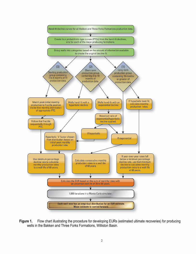
as a flow chart in figure 1. All Bakken and Three Forks Formations horizontal wells with production data were included in this evaluation. Previous USGS assessments used only wells with 19 or more months of production data. The number of months of production data is the basis for determining the specific procedure used to estimate EURs. Wells were separated into three groups by the number of months of production: (1) wells with 19 months or more of production (long-term production group), (2) wells with 5 to 18 months of production (short-term production group), and (3) wells with 1 to 4 months of production (starting production group).

2

Figure 1. Flow chart illustrating the procedure for developing EURs (estimated ultimate recoveries) for producing wells in the Bakken and Three Forks Formations, Williston Basin.

3

These three categories were based in part on the particular behavior of Bakken and Three Forks completions, operations, and well-decline curves. The Bakken and Three Forks horizontal wells are normally produced through a mechanical lift system that is commonly installed after initial completion of the wells. Only after lift equipment is installed can we assume that production is in a stable decline. Even after a hyperbolic decline is interpreted to have begun, there is continuing uncertainty as to when the hyperbolic decline ends.

The production data for each Bakken and Three Forks well were plotted, and the data for each well were “hand-fit” with three points along the temporal-production-data string that allowed us to decide which type of decline-curve function to best extrapolate the data (fig. 2).

Figure 2. Example well showing the positioning of three points that define the initial decline curve in a well with 19 or more months of production data. The positioning of these three points represents the “hand-fit” to production data. Red line signifies the last production-data point in 2012. Year begins with 2008.

The long-term production group consists of wells with 19 or more months of production data

and is interpreted to be the group of wells with the least amount of uncertainty with respect to the “hand-fit” of three points positioned along the temporal data string. Wells having 19 or more months of data have production rates and decline curves that are typically well established. The three main sources of uncertainty within this group are (1) the timing of the failure of the physical wellbore itself, (2) the timing of the depletion of the formation, and (3) the point in time at which the rate of a hyperbolic decline transitions to an exponential decline in the latter stage of the well life.

The short-term production group consists of wells having 5–18 months of data and can exhibit similarities to both the long-term and starting production groups. Uncertainty in this category can lead to

4

a wide range of EUR estimates using the same production data, even among experts using similar methods. The probabilistic system developed for this group accounts for the possibility that the existing production profile is nearly as limited and uncertain as the starting production group, or as certain as the long-term production group.

The starting production group is defined as 1–4 months of production and is designed to require only an approximate well-decline starting point. Using this starting point, a full probabilistic system was developed based on production analogs from wells in that formation with longer temporal-production-data strings, albeit with great uncertainty.

The EURs estimated for all three production groups are for potential oil resources and should not be confused with reserve estimates because no economic criteria were used in the EUR estimation. We assumed that all wells capable of production will continue to produce until some uneconomic rate is reached. No attempt was made to determine what is, or is not, economic production.

EUR Estimation Procedure by Group

Long-Term Production Group The long-term production group (2,954 wells) has the least amount of uncertainty and most

closely resembles a typical decline-curve analysis. A best-fit hyperbolic or exponential decline is fit to existing production data and extrapolated for 60 years (720 months).

Two probabilistic components are added to the long-term production-group fits. The first is the addition of an exponential tail on hyperbolic declines. The well is extrapolated according to the hyperbolic best-fit until the extrapolated decline rate becomes less than a given exponential terminal decline rate. The extrapolation then uses the exponential decline rate to calculate monthly production rates out to 720 months (60 years). The modification of a hyperbolic decline by attaching an exponential tail when a certain rate of decline is reached is referred to as a hybrid-decline model. An overview of stochastic modeling techniques for well-level production using multiple segments of differently declining production data is outlined by Haavardsson and Huseby (2007). The exponential tail method is expected to more accurately reflect the reality of long-term production rates in horizontal Bakken and Three Forks wells in the Williston Basin.

The second probabilistic component is the uncertainty related to the period of time any single well will continue to produce. All production rates in each of the groups were calculated for 720 months, but these data are truncated probabilistically to reflect that not all wells are capable of producing for that length of time. A triangular distribution with a minimum of 240 months (20 years), a mode of 540 months (45 years), and a maximum of 720 months (60 years) is used to represent the distribution of the well or formation failure during the lifespan of the well. In other words, this model represents the chance that any well, on any single iteration, regardless of flow rate, could fail somewhere between 20 to 60 years after the start of production.

A Monte Carlo simulator was used to run 1,000 iterations of this procedure to create an empirical distribution of EURs for each well in the production group. The mean of this distribution was the primary statistical value carried forward for use in the resource assessment.

Short-Term Production Group The short-term production group (1,606 wells) does not contain the most uncertainty of these

decline-curve projections. Wells in this group, however, can be the most misleading if using common deterministic methods to simplify EUR calculations. For example, applying a deterministic decline-type

5

curve or assumed decline parameters and shifting the resulting extrapolation based solely on an initial production point is one of the more common procedures. By definition, EUR will then be singularly dependent upon the starting point. This type of procedure assumes that the increases in initial production are independent of the decline parameters when in fact they are not.

Figure 3 shows hyperbolic exponents (“b” factor) versus initial production rates using data from horizontal wells with enough production to establish a reasonable estimate of hyperbolic behavior. The data in figure 3 were binned and used to create figure 4. The decrease in hyperbolic “b” factor as initial production rate increased is more apparent than in figure 3 and demonstrates why assumptions of independence between initial production and the rest of the parameters used to create deterministic decline parameters or a deterministic decline-type curve are not valid.

Figure 3. Initial monthly production rates compared to hyperbolic “b” factor for wells with more than 24 months of production data.

6

Figure 4. Plot of binned “b” factors compared to initial monthly production rate using data from figure 3. Plot utilized wells with greater than 24 months of production data.

A key difference in the EUR estimation between the short-term production group and the long-

term production group is that there may not be enough data available to make a determination of hyperbolic versus exponential decline. Regardless of whether or not a well has been fit as declining hyperbolically or exponentially, we assume that the past frequency of decline type in wells of Bakken and Three Forks Formations will continue to hold true in the future, including a measure of uncertainty around that ratio.

Wells hand-fit with exponential decline curves are assumed to decline in the same ratio as do wells with known exponential declines in Bakken and Three Forks Formations. The remainder of the time wells are assigned a hyperbolic decline with a “b” factor chosen from the distribution of “b” factors matching initial production rates of those particular wells as provided in figure 4. Wells are extrapolated hyperbolically until the year-to-year decline becomes less than the exponential terminal-decline rate. The same exponential-decline rate that was used on long-term production-group wells was then used to calculate production rates for 720 months.

Wells hand-fit with a hyperbolic decline are assumed to have an amount of uncertainty related to the assigned “b” factor. In each iteration, the “b” factor is chosen from the appropriate “b” factor distribution in figure 4 that matches that well’s initial production rate.

This procedure, in combination with the same well-life truncation that was utilized for long-term production-group wells, is also run through a Monte Carlo simulator 1,000 times to create an empirical distribution of EUR for each well in this production group. The mean of this distribution was the primary statistic carried forward for use in the resource assessment.

Starting Production Group The starting production group (678 wells) involves the most uncertainty of the three groups of

producing wells. Wells within this group are assumed to have established little more than an initial production starting point with a large amount of uncertainty in that starting point. Consistent monthly

7

production from a well could take months to establish because of operational conditions and constraints. These conditions and constraints make it possible for some initial, near-term or partial-production point to be high or low compared to what it would have been under perfect operational conditions and constraints.

To quantify the range of uncertainty in EURs from an initial monthly production point, a full-production performance envelope in the form of a probabilistic-type curve (PTC) was assembled. Assembling a PTC requires that all production information for a given formation be normalized to the number of months from the start of that production. The Anderson-Darling test (Stephens, 1974) is then used to determine the parameters of the distribution for each monthly group. Ordered sequentially from the start of production, this sequence of distributions creates a PTC.

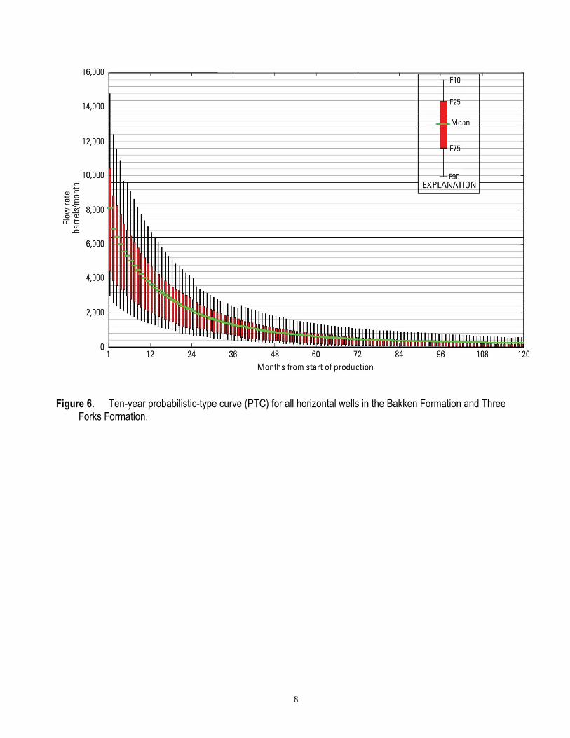
The first 10 years of each PTC used during this procedure are provided in figures 5 through 8. Figure 5 is the PTC for all horizontal wells listed as Bakken Formation producers within the dataset. Figure 6 is the PTC for all horizontal wells listed as producing from the Bakken and Three Forks Formations. Figure 7 is the PTC for all horizontal wells listed as producing from the Three Forks Formation. Figure 8 is the PTC for all horizontal wells listed as producing from the upper part of the Bakken Formation.

Figure 5. Ten-year probabilistic-type curve (PTC) for all horizontal wells in the Bakken Formation.

8

Figure 6. Ten-year probabilistic-type curve (PTC) for all horizontal wells in the Bakken Formation and Three Forks Formation.

9

Figure 7. Ten-year probabilistic-type curve (PTC) for all horizontal wells in the Three Forks Formation.

10

Figure 8. Ten-year probabilistic-type curve (PTC) for all horizontal wells in the upper part of the Bakken Formation.

To create an individual well EUR from a given PTC, the initial monthly production rate is

matched to the corresponding fractile position of the first month distribution of the PTC. The uncertainty around this initial point is then estimated to be one-half of the fractile distance between the initial point and the maximum fractile and one-half the fractile distance between the initial point and the minimum fractile.

Once a starting point within the first monthly PTC distribution has been established, that fractile position is followed consecutively through the formation-specific PTC, assuming perfect positive correlation. Each PTC contains 360 sequential distributions, and when completed, the same exponential terminal-decline rate that was used on wells in the other two production groups is extrapolated for an additional 360 months. The total time frame over which production rates are calculated is 720 months.

This procedure, in combination with the same well-life truncation that was utilized for the other two production groups, was run through a Monte Carlo simulator 1,000 times to create an empirical distribution of EUR for each well in this group. The mean of this distribution was the primary statistic carried forward for use in the resource assessment.

11

EURs by Assessment Unit In 2013 the USGS defined geologic assessment units in the Bakken and Three Forks Formations

in advance of a quantitative resource assessment. We defined six continuous assessment units, five in the Bakken Formation and one in the Three Forks Formation (figs. 9 and 10). Following the estimation of EURs for all Bakken and Three Forks wells, the EURs and wells were assigned to their designated geologically defined assessment unit. Figure 11 represents the full distribution of means of all probabilistic well EURs in each of the six assessment units. The means of these empirical distributions are also shown on figure 11.

Figure 9. Map of five continuous and one conventional assessment units (AU) in the Bakken Formation. TPS, total petroleum system.

12

Figure 10. Map of one continuous and one conventional assessment units (AU) in the Three Forks Formation. TPS, total petroleum system.

13

Figure 11. Family of curves showing the EURs (estimated ultimate recoveries) for five Bakken Formation continuous assessment units (AUs) and one Three Forks Formation continuous AU. MBLS, thousand barrels.

Mean EUR as calculated using the procedures outlined in this paper ranges from 363,000 barrels

for the Eastern Transitional Continuous Oil AU to 148,000 barrels in the Northwest Transitional Continuous Oil AU. Mean EUR for the Three Forks Continuous Oil AU (256,000 barrels) is similar to the mean EUR for several Bakken AUs. These means are useful to quantify historical well productivity and do not represent reserves and are not required to be direct inputs to the geologically based assessment methodology.

Summary This report outlines the procedure by which EURs were estimated for all producing wells in the

Bakken and Three Forks Formations in the Williston Basin. This procedure differs from that used in previous USGS assessments in which wells with 19 or more months of production data were used in the EUR estimation process. The resulting probabilistic EUR distributions were used as guides in the process for estimating EURs for assessment units in the Bakken and Three Forks Formations.

14

References Cited Curtis, John; Kumar, Naresh; Ray, Pulak; Riese, Rusty; and Ritter, John, 2001, American Association of

Petroleum Geologists Committee on Resource Evaluation (CORE) Subcommittee to review the United States onshore continuous (unconventional) gas assessment methodology used by the USGS: Report accessed February 20, 2013, at http://certmapper.cr.usgs.gov/data/noga00/natl/text/core_report.pdf.

Haavardsson, N.F., and Huseby, A.B., 2007, Multisegment production profile models—A tool for enhanced total value chain analysis: Journal of Petroleum Science and Engineering, v. 58, issues 1–2, p. 325–338.

Schmoker, J.W., 1999, U.S. Geological Survey assessment model for continuous (unconventional) oil and gas accumulations—The “FORSPAN” model: U.S. Geological Survey Bulletin 2168, 9 p., accessed January 9, 2013, at http://pubs.usgs.gov/bul/b2168/b2168.pdf.

Stephens, M.A., 1974, EDF statistics for goodness of fit and some comparisons: Journal of American Statistical Association, v. 69, p. 730–737.