proc imeche part d: a robust road bank angle estimation ...acl.kaist.ac.kr/thesis/2012_jae.pdf ·...

Original Article

Proc IMechE Part D:J Automobile Engineering226(6) 779–794� IMechE 2012Reprints and permissions:sagepub.co.uk/journalsPermissions.navDOI: 10.1177/0954407011430919pid.sagepub.com

A robust road bank angle estimationbased on a proportional–integral HN

filter

Jihwan Kim1, Hyeongcheol Lee1 and Seibum Choi2

AbstractThis paper presents a new robust road bank angle estimation method that does not require a differential global position-ing system or any additional expensive sensors. A modified bicycle model, which is less sensitive to model uncertaintiesthan is the conventional bicycle model, is proposed. The road bank angle estimation algorithm designed using this modelcan improve robustness against modelling errors and uncertainties. A proportional–integral HN filter based on the gametheory approach, which is designed for the worst cases with respect to the sensor noises and disturbances, is used asthe estimator in order to improve further the stability and robustness of the bank estimation. The effectiveness and per-formance of the proposed estimation algorithm are verified by simulations and tests, and the results are compared withthose of previous road bank angle estimation methods.

KeywordsRoad bank angle estimation, proportional–integral HN filter, modified bicycle model, observer-based disturbanceestimation

Date received: 24 January 2011; accepted: 14 October 2011

Introduction

Various vehicle chassis control systems have beendeveloped for modern automobiles to meet increasedperformance and safety requirements.1–7 Since the roadvariables, such as the slipperiness, roughness, gradeangle and bank angle, directly affect the vehicledynamics, vehicle chassis control systems can benefitsignificantly by using information about the road vari-ables in real applications, in terms of improved controlaccuracy, robustness and environmental adaptiveness.

Among the road variables, the road bank angle has adirect influence on the lateral and roll dynamics of thevehicle. Therefore, estimation of the road bank anglehas been a significant research topic for vehicle stabilitycontrol,8,9 rollover prevention10–12 and fault manage-ment.12,13 The availability of accurate road bank angleinformation not only improves the accuracy of lateralspeed estimation, which in turn improves the accuracyof stability control,1,2,8,9 but also prevents unnecessaryactivation of vehicle stability control systems when thevehicle is on a banked road.2,8 Road bank angle estima-tion is an essential part of vehicle rollover preventionsystems, because significant road bank angles can createdifferent vehicle roll behaviours during the transient

manoeuvring in which most rollover accidents actuallyoccur.10,12 Road bank angle estimation is also necessaryfor model-based sensor fault detection.12,13

The road bank angle is difficult to measure directlywith commercially available sensors, because it is oftencoupled with other vehicle dynamics in sensor measure-ments, such as the lateral acceleration and the roll andpitch angles of the vehicle. For example, the lateralaccelerometer measurement includes not only the accel-eration of gravity due to the road bank angle but alsothe lateral acceleration.8 In other words, it is difficultto distinguish driving on a banked road from corneringon a flat low-m surface, by using only the lateral accel-erometer measurement.

Several studies have been conducted to explore theestimation of the road bank angle. The road bank

1Department of Electrical and Biomedical Engineering, Hanyang

University, Seoul, Republic of Korea2Department of Mechanical Engineering, Korea Advanced Institute of

Science and Technology, Daejeon, Republic of Korea

Corresponding author:

Hyeongcheol Lee, Department of Electrical and Biomedical Engineering,

Hanyang University, Seoul 133-791, Republic of Korea.

Email: [email protected]

angle and modelling errors are defined as uncertainparameters and they are estimated using a disturbanceobserver10 and the adaptive control theory.14 Theseestimation methods require the side-slip angle, whichcan be estimated using the differential global position-ing system (DGPS) measurement. Different from theone-antenna global positioning system (GPS), which isgenerally used in automotive navigation systems, theDGPS with two antennae is too expensive to be used inpassenger cars and is frequently unreliable in urbanenvironments.9 Even though these methods can guar-antee an acceptable accuracy of estimation, they arenot practical solutions owing to the cost and reliabilityissues related to the DGPS. A road bank angle estima-tion using a vertical accelerometer is proposed.9

However, the vertical accelerometer measurementalso cannot provide an acceptable accuracy of theroad bank angle because the vertical accelerometer isalmost insensitive to the narrow range of vehicle tiltsowing to the non-linearity of the arccosine functionalrelation between the vertical acceleration and the vehi-cle tilt.15

The road bank angle has been estimated using thedifferences between the lateral tyre force estimate andthe lateral accelerometer measurement,16 or the differ-ences between the lateral acceleration measurement andthe products of the yaw rate and the longitudinalspeed17 in the linear observer framework. However,these methods tend to be inaccurate under transientdriving conditions because they neglect the derivativeterm of the lateral velocity of the vehicle. A road bankangle estimation method based on the transfer functionand dynamic filter compensation (DFC), which isrelated to the model uncertainty of the lateral dynamics,was previously introduced.8,12 This method illustratedthe robustness issues of the road bank angle estimation;however, the physical meaning of the DFC term wasnot explicitly explained in the papers.

Disturbance observers based on the unknown inputobserver (UIO), which is a well-known solution forthe state and disturbance estimation of linear systems,were proposed to estimate the road bank angle.13,18

This method can guarantee the stability and conver-gence of the estimation error, but estimation by thismethod is sensitive to the output changes because ofthe derivative term of the output in the observer.More complex methods that consider the rolldynamics of vehicles19,20 were developed in order toestimate the roll angle of the vehicle and the roadbank angle individually. On the other hand, non-lin-ear modelling and table-based estimation methods21

were developed in order to improve the accuracy of thestate estimation of the lateral dynamics. However, mostof the previous road bank angle estimation methodsexplained above did not address the robustness issue ofthe estimation due to uncertainties and disturbances,such as the cornering stiffnesses of the tyres and thechanges in the vehicle mass.

This paper presents a new robust road bank angleestimation method that does not require DGPS or any

additional expensive sensors. A modified bicycle model,which is less sensitive to model uncertainties such asthe cornering stiffnesses of the tyres than is the conven-tional bicycle model, is proposed in this paper.Therefore, the road bank angle estimation algorithmdesigned using this model can be more robust againstmodelling errors and uncertainties than using the con-ventional bicycle model. A proportional–integral HN

filter (PIF) based on the game theory approach, whichis designed for the worst cases with respect to the sen-sor noises and disturbances, is used as the estimator inorder to improve further the stability and robustness ofthe bank estimation. The effectiveness and performanceof the proposed estimation algorithm are verified bysimulations and tests, and the results are comparedwith those of previous road bank angle estimationmethods.

Vehicle dynamics model

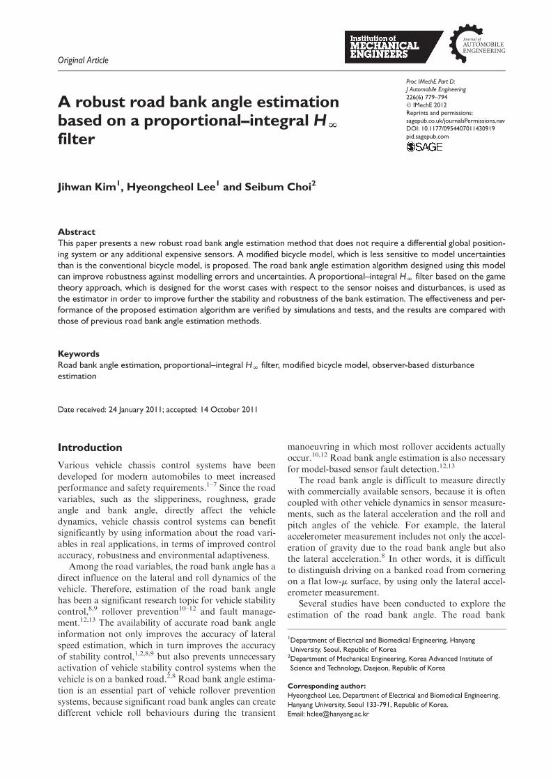
Figure 1 shows the schematic diagrams of the targetsystem. As shown in Figure 1(a), by assuming thebicycle model (i.e. by assuming that the dynamics ofthe left and right sides of the vehicle are identical) andno pitch motion, the lateral motion of the vehicle22,23

can be expressed by

may =Fyf+Fyr

Iz€c=LfFyf � LrFyr ð1Þ

The lateral accelerometer measurement consists of threecomponents, namely the linear motion term, the lateralmotion term and the gravity term, according to22

ay = _vy + vx _c+ g sin (fb +f) ð2Þ

where fb is the road bank angle and f is the roll angleof the vehicle. By equation (2), it is shown that the lat-eral acceleration measurement includes not only thedynamic component _vy + vxr of the vehicle motion butalso the gravity component g sin (fb +f) of the roadbank angle and the roll angle. By assuming that the lat-eral forces of the tyres are linearly proportional to thecornering stiffnesses of the tyres and that the slip anglesof the tyres are very small, the lateral force of each tyrecan be expressed as22,23

Fyf ’�Cfaf = �Cf(bf � df)

Fyr ’�Crar = �Crbr

bf =tan�1vy +Lf

_c

vx

� �’

vy +Lf_c

vx

br =tan�1vy � Lr

_c

vx

� �’

vy � Lr_c

vx

Cf =∂Fyf

∂af

��af =0

, Cr =∂Fyr

∂ar

��ar =0 ð3Þ

For simplification, let u=fb +f. From equations (1),(2) and (3), the lateral and yaw motions of a vehicle areexpressed by the state equations

780 Proc IMechE Part D: J Automobile Engineering 226(6)

_x=Aox+Bouo +Eow

yo =Cox+Douo ð4Þ

where

x=vy_c

� �, yo =

ay_c

� �uo = df, w= sinu

Ao =� Cf +Cr

mvx� LfCf�LrCr

mvx� vx

� LfCf�LrCr

Izvx� L2

fCf +L2

r Cr

Izvx

0@

1A

Bo =

Cf

m

LfCf

Iz

!

Co =� Cf +Cr

mvx� LfCf�LrCr

mvx

0 1

!

Do =Cf

m

0

!, Eo =

�g0

� �

The mathematical model expressed by equations (4)does not fully agree with the actual system owing to theinevitable model uncertainties. Specifically, the modellingerror in the cornering stiffnesses Cf and Cr, which resultsfrom the linear lateral force assumption and the small-side-slip-angle assumption, is one of the major causes ofthe model uncertainties. Moreover, the lateral forces ofthe front tyres of a front-wheel-drive vehicle are affectednot only by the side-slip angles but also by the tractionforces. Therefore, the cornering stiffness of the front tyresof a front-wheel-drive vehicle may incur more model inac-curacies than that of the rear tyres during the traction. Amodified vehicle model describing more accurate vehiclelateral and yaw motions can be obtained by eliminatingthe cornering stiffness terms of the front tyres from thevehicle’s lateral equations of motion. From equation (2)and the second equation of equation (1), the equationswhich do not include the Fyf term can be obtained as

_vy = ay � vx _c� g sinu

Iz€c =Lfmay � (Lf +Lr)Fyr ð5Þ

From equations (5) and (3), the state equations of themodified vehicle dynamic model can be obtained as

_x=Amx+Bmum +Emw

ym =Cmx ð6Þ

where

x=vy_c

� �, um = ay, w= sinu

Am =0 �vx

(Lf +Lr)Cr

Izvx� (Lf +Lr)LrCr

Izvx

!

Bm =1

Lfm

Iz

!

Cm = 0 1ð Þ, Em =�g0

� �

As shown in equations (6), the modified model is notaffected by the cornering stiffness of the front tyres.Therefore, it can be said that the modified model is lesssensitive to variations in the cornering stiffnesses of thetyres than is the conventional bicycle model, and the roadbank angle estimation designed using the modified modelcan be more robust against the uncertainties. Similaranalyses can be conducted for rear-wheel-drive vehiclesby eliminating the cornering stiffness terms of the reartyres from the equations of motion of the vehicle.

Robustness analysis of the estimationmethods

As commented in the previous section, variations in thecornering stiffnesses of the tyres exist under real drivingconditions and they make the parameters of the vehiclemodel uncertain. For this reason, the effects of theparameter uncertainties on the estimation errors should

(a)

(b)

(c)

xv

fα

fδaxisx

Rear tyre Front tyre

xvrα

axisx

mg

bϕ

h

bφφ

CG

ya

axisy

axisz

fLrL

yrF yfFrαfα

xv

fδψ�

ya

axisy

axisx

Figure 1. Schematic diagrams of the target system: (a) bicyclemodel of a vehicle; (b) rear view of a vehicle; (c) tyre diagram.CG: centre of gravity.

Kim et al. 781

be analysed in order to improve the robustness of theestimation.

In this section, four estimation methods derivedfrom equations (4) or equations (6) are explained andanalysed in order to compare the robustness of the esti-mation methods against modelling errors and uncer-tainties and, in particular, the modelling error in thecornering stiffnesses Cf and Cr.

For clarity, the uncertainties in the cornering stiff-nesses are denoted DCf and DCr in this paper. Theuncertainties in the system matrices of the original vehi-cle dynamic model (4) can be expressed by using DCf

and DCr as

DAo =� DCf +DCr

mvx� Lf DCf�Lr DCr

mvx

� Lf DCf�Lr DCr

Izvx� L2

fDCf +L2

r DCr

Izvx

0@

1A

DBo =

DCf

m

Lf DCf

Iz

!

DCo =� DCf +DCr

mvx� Lf DCf�Lr DCr

mvx

0 0

!

DDo =DCf

m

0

� �ð7Þ

On the other hand, for the modified vehicle dynamicmodel (6), the uncertainties in the system matrices canbe expressed as

DAm =0 0

(Lf +Lr) DCr

Izvx� (Lf +Lr)Lr DCr

Izvx

!

DBm =0

DCm =0 0

0 0

� �

DDm =00

� �ð8Þ

Dynamic filter compensation method

If the derivative of the lateral speed is zero (i.e. _vy =0),the road bank angle estimation can be derived fromequation (2) as

sin uv =ay � vx _c

gð9Þ

Estimating the road bank angle based on equation (9)simplifies the calculation of the estimation, but the esti-mation becomes more inaccurate as _vy

�� becomes larger.The DFC method8 was proposed to relieve this problemby compensating equation (9) with the DFC term,according to

wdfc= sin uv max 0, 1� jDFCj � d

dtsin uv

��

� �ð10Þ

where

DFC(s)=Haw½sin ua(s)� sin uv(s)�+ vxHrw½sin ur(s)� sin uv(s)�

sin ua(s)=Haw�1½Ay(s)�HauUo(s)�

sin ur(s)=Hrw�1½ _C(s)�HruUo(s)�

Hau

Hru

� �=Co(sI� Ao)

�1Bo +Do

Haw

Hrw

� �=Co(sI� Ao)

�1Eo

If the model uncertainties do not exist, Ay(s)=HauUo(s)+HawW(s) and _C(s)=HruUo(s)+HrwW(s).This yields

DFC(s)=HawW(s)+ vxHrwW(s)

� (Haw + vxHrw)½Ay(s)� vx _C(s)�g

=�(Haw+ vxHrw)½�gW(s)+Ay(s)� vx _C(s)�

g

=�(Haw+ vxHrw)sVy(s)

g

ð11Þ

In equation (11), (Haw+ vxHrw)=g is a form ofsecond-order low-pass filter and therefore DFC can beconsidered as an estimation of _vy. If the model uncer-tainties exist, the transfer functions of equations (4) canbe expressed as

�Hau

�Hru

� �=(Co +DCo)(sI� Ao � DAo)

�1(Bo +DBo)

+Do +DDo

�Haw

�Hrw

� �=(Co +DCo)(sI� Ao � DAo)

�1Eo

ð12Þ

Then, the uncertainties in the transfer functions are

DHau= �Hau �Hau, DHru= �Hru �Hru

DHaw= �Haw �Haw, DHrw= �Hrw �Hrw ð13Þ

In this case, the DFC can be obtained as

DFC(s)=HawW(s)+ vxHrwW(s)

� (Haw + vxHrw)½Ay(s)� vx _C(s)�g

+DHau Uo(s)+DHaw W(s)+ vx DHru Uo(s)

+ vx DHrw W(s)

=�(Haw+ vxHrw)sVy(s)

g+(DHau+ vx DHru)Uo(s)

+ (DHaw + vx DHrw)W(s)

ð14Þ

Equation (14) implies that the model uncertaintiesmake the DFC inaccurate from the viewpoint of the _vyestimation because DHau+vxDHru and DHaw+vxDHrw


are non-zero even if the system is in a steady state. Forthis reason, wdfc has steady state errors if uo or w arenot zero.

It was proposed by Tseng8 that the steady state val-ues of the transfer functions Haw and vxHrw are actuallyimplemented for the actual automotive applications tomitigate the computational burden, according to

lims!0

Haw = � g(Lf +Lr)

(Lf +Lr)+Kusv2x

lims!0

vxHrw =gKusv

2x

(Lf +Lr)+Kusv2x ð15Þ

where

Kus=Lrm

(Lf +Lr)Cf� Lfm

(Lf +Lr)Cr

Unknown input observer method

The UIO is a state observer designed to decouple thestate estimation error from the disturbance.24 The dis-turbance can be estimated by using the state estima-tion of the UIO. The form of the UIO13,18 is expressedby

_zuio=Nuiozuio+Luioyuio+Guiouo

xuio= zuio � Euioyuio ð16Þ

where

yuio= yo �Douo

Nuio, Luio, Guio and Euio can be designed by the fol-lowing steps. The derivative of xuio can be derived fromequations (4) and (16) as

_xuio= _zuio � EuioCo _x

=Nuiozuio+Luioyo +(Guio � LuioDo)uo

� EuioCo(Aox+Bouo +Eow) ð17Þ

If the model uncertainties do not exist, the dynamics ofthe estimation error are given by

_x� _xuio=(I+EuioCo)(Aox+Bouo+Eow)�Nuiozuio � Luioyo

� (Guio � LuioDo)uo

= ½(I+EuioCo)Ao �MuioCo�(x� xuio)+MuioCox

+ ½(I+EuioCo)Ao �MuioCo�xuio +(I+EuioCo)Bouo

+(I+EuioCo)Eow�Nuiozuio � Luioyo � (Guio � LuioDo)uo

= ½(I+EuioCo)Ao �MuioCo�(x� xuio)

+ ½(I+EuioCo)Ao �MuioCo �Nuio�zuio+ ½�(I+EuioCo)AoEuio+MuioCoEuio +Muio � Luio�yo+ f½(I+EuioCo)Ao �MuioCo�EuioDo +(Luio �Muio)Do

+(I+EuioCo)Bo � Guioguo +(I+EuioCo)Eow

ð18Þ

where Muio is a constant matrix, which should beselected to make (I+EuioCo)Ao �MuioCo stable. In

order to make equation (18) asymptotically stable (i.e.limt!‘(x� xuio)=0), the equations that should bevalid are

Euio= �Eo(CoEo)þ+Quio½I� CoEo(CoEo)

þ�Nuio=(I+EuioCo)Ao �MuioCo

Luio= �NuioEuio+Muio

Guio=(I+EuioCo)Bo ð19Þ

Quio is a constant matrix, which consists of designparameters and (CoEo)

þ is the left inverse of CoEo

(i.e. ½(CoEo)TCoEo��1(CoEo)

T). The estimation ofw based on the UIO was proposed by Imsland et al.18

as

wuio=Eþo ½Luioyuio � Euio _yuio

�(LuioCo � EuioCoAo)xuio +EuioCoBouo� ð20Þ

If the model uncertainties do not exist,

Eo(w� wuio)=Eow� LuioCox+EuioCo(Aox+Bouo +Eow)

+ (LuioCo � EuioCoAo)xuio � EuioCoBouo

=(EuioCoAo � LuioCo)(x� xuio)+ (I+EuioCo)Eow

=(EuioCoAo � LuioCo)(x� xuio)

ð21Þ

This shows that equation (20) was designed to achievelimt!‘wuio =w by using limt!‘(x� xuio)=0 but, if themodel uncertainties exist, the derivative of xuio is chan-ged to

_xuio= _zuio � Euio(Co +DCo) _x� Euio DDo _uo

=Nuiozuio+Luioyo +(Guio � LuioDo)uo

� Euio(Co +DCo)(Aox+DAo x+Bouo

+DBouo +Eow)� Euio DDo _uo ð22Þ

Then, the error dynamics of the UIO are given by

_x� _xuio=(I+EuioCo +Euio DCo)(Aox+DAo x

+Bouo +DBouo +Eow)

�Nuiozuio � Luioyo � (Guio � LuioDo)uo

+Euio DDo _uo

=Nuio(x� xuio)+MuioCox+Nuioxuio

�Nuiozuio � Luioyo +LuioDouo

+Euio DCo (Aox+DAo x+Bouo +DBo uo +Eow)

+ (I+EuioCo)(DAo x+DBo uo)+Euio DDo _uo

=Nuio(x� xuio)+Euio DCo Eow+Euio DDo _uo

+ ½(I+EuioCo) DAo �Muio DCo

+Euio DCo (Ao +DAo)�x+ ½(I+EuioCo) DBo �Muio DDo

+Euio DCo (Bo +DBo)�uoð23Þ

This means that limt!‘(x� xuio) 6¼ 0 if the modeluncertainties exist. The error of wuio is

Kim et al. 783

Eo(w� wuio)=Eow� Luio(Co +DCo)x� Luio DDo uo

+EuioCo(Aox+DAo x+Bouo

+DBo uo +Eow)

+ (LuioCo � EuioCoAo)xuio � EuioCoBouo

=(EuioCoAo � LuioCo)(x� xuio)

+ (EuioCo DAo � Luio DCo)x

+(EuioCo DBo � Luio DDo)uo

ð24Þ

Therefore, it is concluded that the model uncertain-ties make both xuio and wuio inaccurate and wuio hassteady state errors if x or uo are not zero.

Because differentiating the output amplifies theeffect of the sensor noise, a low-pass filter is used in thispaper according to

_yuio(s)=s

tuios+1yuio(s) ð25Þ

where tuio is the time constant of the filter.

Proportional–integral observer of the originalvehicle dynamic model

The proportional–integral observer (PIO) is a stateobserver designed to reduce the steady state error byusing one or more integration terms of the estimationerror.25,26 A PIO can be derived from the original vehi-cle dynamic model (4) as

_xpo =Aoxpo +Bouo +Kpo1(yo � yo)+Eowpo

_wpo =Kpo2(yo � yo), yo =Coxpo +Douo ð26Þ

where Kpo1 and Kpo2 are the observer gain matrices. Ifthe model uncertainties do not exist, the dynamics ofthe estimation error are given by

_x� _xpo =(Ao � Kpo1Co)(x� xpio)+Eo(w� wpo)

_w� _wpo= �Kpo2Co(x� xpo)+ _w

ð27Þ

This means that Kpo1 and Kpo2 should be selectedto make Ao � Kpo1Co and Kpo2Co stable. If themodel uncertainties exist, the error dynamics of thePIO derived from the original model are changedto

_x� _xpo=(Ao � Kpo1Co)(x� xpo)+Eo(w� wpo)

+ (DAo x+DBo uo)� Kpo1(DCo x+DDo uo)

_w� _wpo=�Kpo2Co(x� xpo)+ _w� Kpo2(DCo x

+DDo uo)

ð28Þ

If the time goes to infinity, the error dynamics of thePIO become

limt!‘

x� xpow� wpo

� �=

Ao � Kpo1Co Eo

�Kpo2Co 0

� ��1

3Kpo1 �IKpo2 0

� �DCo x+DDo uoDAo x+DBo uo

� �ð29Þ

It is possible to select Kpo1 and Kpo2 to minimize equa-tion (29) at the cost of reducing the freedom of theobserver design (e.g. pole placement methods should bemodified in order to minimize equation (29)). However,variations in the other vehicle parameters are ignoredin equation (29) and they can amplify the steady stateerror of the estimation even if equation (29) is mini-mized by the gain selection.

PIO of the modified vehicle dynamicmodel

A PIO can be derived from the modified vehicledynamic model (6) according to

_xpm =Amxpm +Bmum +Kpm1(ym � ym)+Emwpm

_wpm=Kpm2(ym � ym), ym =Cmxpm

ð30Þ

where Kpm1 and Kpm2 are the observer gain matrices. Ifthe model uncertainties exist, the error dynamics of thePIO of the modified model are given by

_x� _xpm=(Am�Kpm1Cm)(x� xpm)+Em(w� wpm)+DAm x

_w� _wpm= �Kpm2Cm(x� xpm)+ _w

ð31Þ

If the time goes to infinity

limt!‘

(w� wpm)= 0 Ið Þ Am � Kpm1Cm Em

�Kpm2Cm 0

� ��1

3�DAm x

0

� �=0 ð32Þ

Therefore, it is concluded that the PIO of the modi-fied model can eliminate the steady state error of wpm

even if DAm exists. It is notable that the steady stateerror remains zero even if variations in the other vehicleparameters exist owing to the structure of equations(6).

Proposed road bank angle estimationmethod

The results of the previous section show that the PIOderived from the modified model is the best solutionfrom the viewpoint of the robust performance of thesteady state error. This paper proposes to apply thePIO algorithm to the bank angle estimation using themodified vehicle model (6). By assigning w= sinu as anew state, equations (6) can be modified as


_xw =Awxw +Bwum +Ewn

ym =Cwxw + v

w=Lwxw ð33Þ

where

xw =

vy_c

w

0B@

1CA, n=

d

dtsinu

Aw =

0 �vx �g(Lf +Lr)Cr

Izvx� (Lf +Lr)LrCr

Izvx0

0 0 0

0B@

1CA

Bw =

1Lfm

Iz

0

0B@

1CA, Cw = 0 1 0ð Þ

Ew =

0

0

1

0B@

1CA, Lw = 0 0 1ð Þ

and v is the noise in the yaw rate measurement such asoffset and stiction.27 It is notable that the Luenbergerobserver derived from equations (33) is the same as thePIO in equations (30).

Because the rank of the observability matrix of thesystem described by equations (33) is

rank Cw CwAw CwA2w

� �T=3 ð34Þ

the system described by equation (34) is observable.In order to make the observer derived from equa-

tions (33) robust against a set of disturbances includingthe disturbance term n and the noise term v, this paperproposes to use a continuous-time HN filter based onthe game theory approach.28–30 The error of the roadbank angle estimation is

ew =w� w ð35Þ

where w is the estimation of the road bank angle term.Because the input um and the output ym are the onlyknown terms, the estimate of the road bank angle termshould be derived from them. Let

w=Lwxw

xw = fest(um, ym, xw(0))ð36Þ

where fest(um, ym, xw(0)) is the estimation function, whichshould be determined. From equations (33), (35) and(36), the estimation error at time 0 can be derived as

ew(0)=w(0)� w(0)

=Lw½xw(0)� xw(0)� ð37Þ

On the basis of equations (33), (35), (36) and (37), it canbe said that the estimation error ew is a function of n, vand xw(0)� xw(0). Therefore, ew can be expressed as

ew(s)=Gerr(s)e(s) ð38Þ

where e= n v xw(0)� xw(0)ð ÞT. The robustness ofthe estimation can be achieved by ensuring that ewk k‘

is less than a certain value.30 The system N-norm ofGerr is defined as31

Gerrk k‘ = supe6¼0

ffiffiffiffiffiffiffiffiffiffiffiffiffiffiffiffiffiffiffiffiffiÐ tf0 ewk k dtÐ tf0 ek k dt

vuut

= supe6¼0

ffiffiffiffiffiffiffiffiffiffiffiffiffiffiffiffiffiffiffiffiffiffiffiffiffiffiffiffiffiffiffiffiffiffiffiffiffiffiffiffiffiffiffiffiffiffiffiffiffiffiffiffiffiffiffiffiffiffiffiffiffiffiffiffiffiffiffiffiffiffiffiffiffiffiffiffiffiffiffiffiffiffiffiffiffiffiffiffiffiffiffiffiffiffiffiffiffiffiffiffiffiffiffiffiffiÐ tf0 (w� w)T(w� w) dt

½xw(0)� xw(0)�T½xw(0)� xw(0)�+Ð tf0 (nTn+ vTv) dt

vuutð39Þ

where sup stands for supremum. Because the goal oftheH‘ filter is to make Gerrk k‘ less than a certain value,the cost function of the H‘ filter is defined as28–30

Jw = Ð tf0 (w� w)TS(w� w) dt

½xw(0)� xw(0)�TP0�1½xw(0)� xw(0)�+

Ð tf0 (nTQ�1n+ vTR�1v) dt

ð40Þ

where P0, Q, R and S are positive definite matrices thatdepend on the performance requirements. Because allthe state equation matrices of equations (33) are contin-uous, the system N-norm Gerrk k‘ is finite.31 This meansthat there exists a positive scalar u such that the optimalestimation w satisfies

supe6¼0

Jw41

uð41Þ

Conditions of the existence of a bound on thesystem N-norm Gerrk k‘ and the lower bound of theN-norm can be derived using theorems given byBurl;31 therefore the upper bound of u can also bederived.30 The derivation of the upper bound of u isomitted because it is beyond the scope of this paper.The continuous-time H‘ filter can be derived fromequation (41) as

_xw =Awxw +Bwum +PCTwR�1(ym � Cwxw) ð42Þ

where

w=Lwxw, xw(0)= xw0

and as

_P=AwP+PATw +EwQET

w

�P(CTwR�1Cw � uLT

wSLw)P ð43Þ

where

P(0)=P0

and P is a symmetric positive definite matrix if thesolution of equation (43) exists 8t 2 ½0, tf�. Thedetailed derivations of equations (42) and (43) can befound in the papers by Banavar and Speyer28 and deSouza et al.29 It is notable that the solution of thealgebraic Riccati form of equation (43) can be used as

Kim et al. 785

P0 in order to reduce the calculation complexity ofequation (43) by taking the risk of increasing the esti-mation errors due to the initial state xw(0).

30 In thiscase, the steady-state HN filter can be obtained fromequations (42) and (43) as

_xw =Awxw +Bwum +P0CTwR�1(ym � Cwxw)

AwP0 +P0ATw +EwQET

w

�P0(CTwR�1Cw � uLT

wSLw)P0 =0 ð44Þ

where

w=Lwxw, xw(0)= 0 0 0ð ÞT

Since w= sin fb +fð Þ, the roll angle estimation f isnecessary in order to separate the road bank angle esti-mation from w. The roll angle can be estimated using avehicle-dynamics-based roll estimation method.32

Simulation results

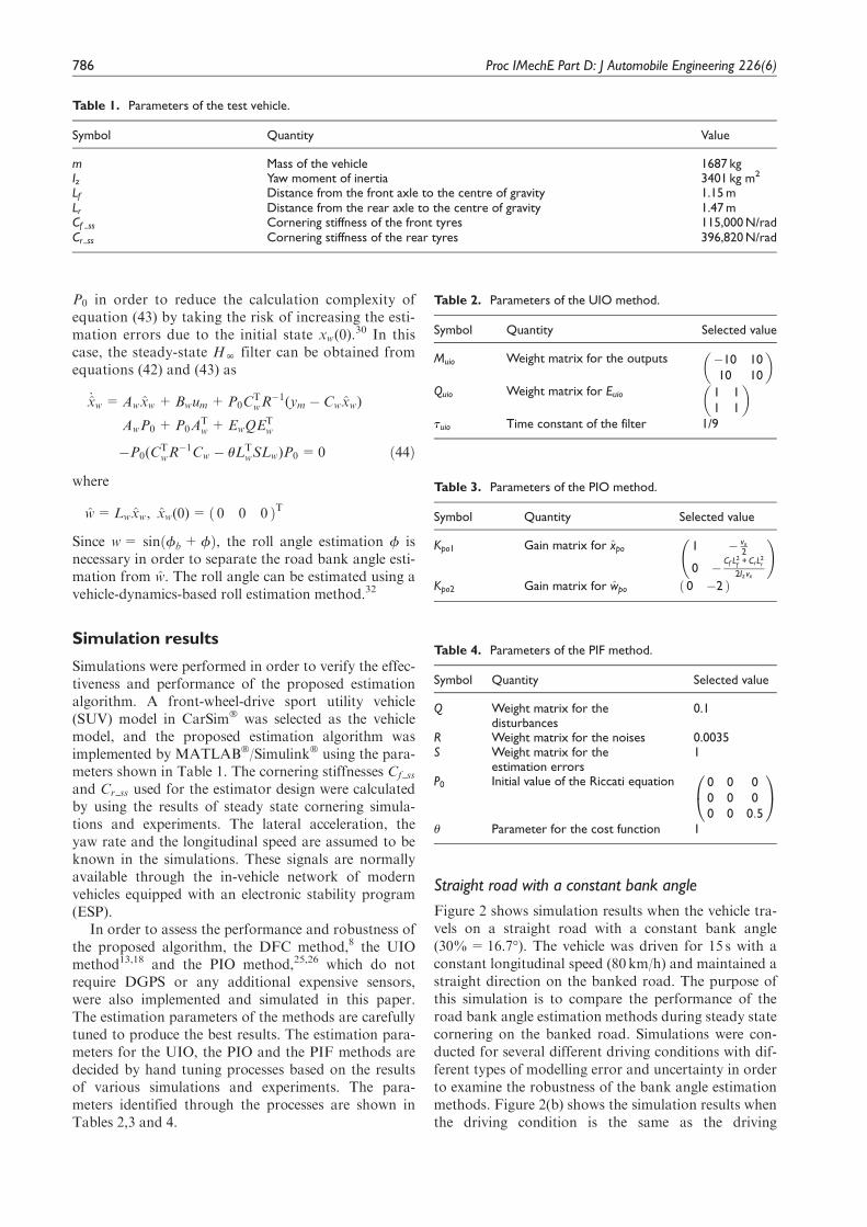
Simulations were performed in order to verify the effec-tiveness and performance of the proposed estimationalgorithm. A front-wheel-drive sport utility vehicle(SUV) model in CarSim� was selected as the vehiclemodel, and the proposed estimation algorithm wasimplemented by MATLAB�/Simulink� using the para-meters shown in Table 1. The cornering stiffnesses Cf ss

and Cr ss used for the estimator design were calculatedby using the results of steady state cornering simula-tions and experiments. The lateral acceleration, theyaw rate and the longitudinal speed are assumed to beknown in the simulations. These signals are normallyavailable through the in-vehicle network of modernvehicles equipped with an electronic stability program(ESP).

In order to assess the performance and robustness ofthe proposed algorithm, the DFC method,8 the UIOmethod13,18 and the PIO method,25,26 which do notrequire DGPS or any additional expensive sensors,were also implemented and simulated in this paper.The estimation parameters of the methods are carefullytuned to produce the best results. The estimation para-meters for the UIO, the PIO and the PIF methods aredecided by hand tuning processes based on the resultsof various simulations and experiments. The para-meters identified through the processes are shown inTables 2,3 and 4.

Straight road with a constant bank angle

Figure 2 shows simulation results when the vehicle tra-vels on a straight road with a constant bank angle(30%=16.7�). The vehicle was driven for 15 s with aconstant longitudinal speed (80km/h) and maintained astraight direction on the banked road. The purpose ofthis simulation is to compare the performance of theroad bank angle estimation methods during steady statecornering on the banked road. Simulations were con-ducted for several different driving conditions with dif-ferent types of modelling error and uncertainty in orderto examine the robustness of the bank angle estimationmethods. Figure 2(b) shows the simulation results whenthe driving condition is the same as the driving

Table 1. Parameters of the test vehicle.

Symbol Quantity Value

m Mass of the vehicle 1687 kgIz Yaw moment of inertia 3401 kg m2

Lf Distance from the front axle to the centre of gravity 1.15 mLr Distance from the rear axle to the centre of gravity 1.47 mCf ss Cornering stiffness of the front tyres 115,000 N/radCr ss Cornering stiffness of the rear tyres 396,820 N/rad

Table 4. Parameters of the PIF method.

Symbol Quantity Selected value

Q Weight matrix for thedisturbances

0.1

R Weight matrix for the noises 0.0035S Weight matrix for the

estimation errors1

P0 Initial value of the Riccati equation 0 0 00 0 00 0 0:5

0@

1A

u Parameter for the cost function 1

Table 2. Parameters of the UIO method.


Muio Weight matrix for the outputs �10 1010 10

� �Quio Weight matrix for Euio 1 1

1 1

� �tuio Time constant of the filter 1/9

Table 3. Parameters of the PIO method.


Kpo1 Gain matrix for xpo 1 � vx

2

0 � Cf L2f

+ CrL2r

2Izvx

!

Kpo2 Gain matrix for wpo 0 �2ð Þ


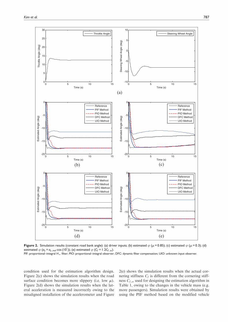
condition used for the estimation algorithm design.Figure 2(c) shows the simulation results when the roadsurface condition becomes more slippery (i.e. low m).Figure 2(d) shows the simulation results when the lat-eral acceleration is measured incorrectly owing to themisaligned installation of the accelerometer and Figure

2(e) shows the simulation results when the actual cor-nering stiffness Cf is different from the cornering stiff-ness Cf ss used for designing the estimation algorithm inTable 1, owing to the changes in the vehicle mass (e.g.more passengers). Simulation results were obtained byusing the PIF method based on the modified vehicle

0 5 10 150

5

10

15

20

25

30

Thr

ottle

Ang

le (

deg)

Time (s)

Throttle Angle

0 5 10 15-15

-10

-5

0

5

10

Ste

erin

g W

heel

Ang

le (

deg)

Time (s)

Steering Wheel Angle

(a)

0 5 10 15-20

-15

-10

-5

0

Est

imat

ed A

ngle

(de

g)

Time (s)

Reference

PIF Method

PIO MethodDFC Method

UIO Method

0 5 10 15-20

-15

-10

-5

0

Est

imat

ed A

ngle

(de

g)

Time (s)

Reference

PIF Method


UIO Method

(b) (c)

0 5 10 15-20

-15

-10

-5

0

Est

imat

ed A

ngle

(de

g)

Time (s)

Reference

PIF Method


UIO Method

0 5 10 15-20

-15

-10

-5

0

Est

imat

ed A

ngle

(de

g)

Time (s)

Reference

PIF Method


UIO Method

(d) (e)

Figure 2. Simulation results (constant road bank angle): (a) driver inputs; (b) estimated u (m = 0:85); (c) estimated u (m = 0:3); (d)estimated u (ay = ay real cos (108)); (e) estimated u (Cf = 1:2Cf ss).PIF: proportional–integral HN filter; PIO: proportional–integral observer; DFC: dynamic filter compensation; UIO: unknown input observer.

Kim et al. 787

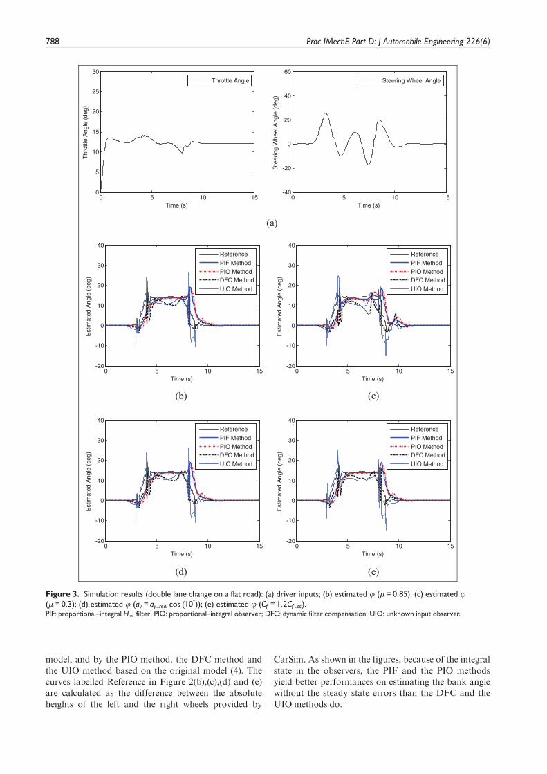
model, and by the PIO method, the DFC method andthe UIO method based on the original model (4). Thecurves labelled Reference in Figure 2(b),(c),(d) and (e)are calculated as the difference between the absoluteheights of the left and the right wheels provided by

CarSim. As shown in the figures, because of the integralstate in the observers, the PIF and the PIO methodsyield better performances on estimating the bank anglewithout the steady state errors than the DFC and theUIO methods do.

0 5 10 150

5

10

15

20

25

30

Thr

ottle

Ang

le (

deg)

Time (s)

Throttle Angle

0 5 10 15-40

-20

0

20

40

60

Ste

erin

g W

heel

Ang

le (

deg)

Time (s)


(a)

0 5 10 15-20

-10

0

10

20

30

40

Est

imat

ed A

ngle

(de

g)

Time (s)

Reference

PIF Method


UIO Method

0 5 10 15-20

-10

0

10

20

30

40

Est

imat

ed A

ngle

(de

g)

Time (s)

Reference

PIF Method


UIO Method

(b) (c)

0 5 10 15-20

-10

0

10

20

30

40

Est

imat

ed A

ngle

(de

g)

Time (s)

Reference

PIF Method


UIO Method

0 5 10 15-20

-10

0

10

20

30

40

Est

imat

ed A

ngle

(de

g)

Time (s)

Reference

PIF Method


UIO Method

(d) (e)

Figure 3. Simulation results (double lane change on a flat road): (a) driver inputs; (b) estimated u (m = 0:85); (c) estimated u(m = 0:3); (d) estimated u (ay = ay real cos (108)); (e) estimated u (Cf = 1:2Cf ss).PIF: proportional–integral HN filter; PIO: proportional–integral observer; DFC: dynamic filter compensation; UIO: unknown input observer.


0 5 10 15 20 250

5

10

15

20

25

30

Thr

ottle

Ang

le (

deg)

Time (s)

Throttle Angle

0 5 10 15 20 25-400

-300

-200

-100

0

100

200

300

400

Ste

erin

g W

heel

Ang

le (

deg)

Time (s)


(a)

0 5 10 15 20 25-20

-15

-10

-5

0

5

10

15

20

Est

imat

ed A

ngle

(de

g)

Time (s)

Reference

PIF Method


UIO Method

0 5 10 15 20 25-20

-15

-10

-5

0

5

10

15

20

Est

imat

ed A

ngle

(de

g)

Time (s)

Reference

PIF Method


UIO Method

(b) (c)

(d) (e)

0 5 10 15 20 25-20

-15

-10

-5

0

5

10

15

20

Est

imat

ed A

ngle

(de

g)

Time (s)

100% Cf

150% Cf50% Cf

0 5 10 15 20 25-20

-15

-10

-5

0

5

10

15

20

Est

imat

ed A

ngle

(de

g)

Time (s)

100% Cf

150% Cf50% Cf

Figure 4. Simulation results (S-curve manoeuvre on a flat road): (a) driver inputs; (b) estimated u (m = 0:85); (c) estimated u(m = 0:3); (d) robustness of PIF with the modified vehicle model (m = 0:85); (e) robustness of PIF with the original vehicle model(m = 0:85).PIF: proportional–integral HN filter; PIO: proportional–integral observer; DFC: dynamic filter compensation; UIO: unknown input observer.

Kim et al. 789

Bank angle change on a straight road

Figure 3 shows the simulation results when the vehicletravels on a straight road with two lanes, flat andbanked (25%=14�) lane, and changes lanes. Figure3(a) shows the driving manoeuvre. The purpose of thissimulation is to compare the performances of the roadbank angle estimation methods when the road bankangle is changed. Similar to the constant-bank-anglecase, simulations were conducted for several differentdriving conditions with different types of modellingerror and uncertainty. The simulation results show thatthe modified-model-based PIF method yields the bestperformance and robustness in estimating the roadbank angle and maintains its accuracy even in the pres-ence of the model uncertainties.

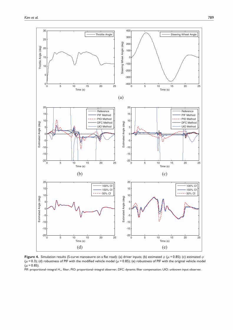
S-curve manoeuvre on a flat road

Figure 4 shows the simulation results when the vehicletravels on a flat road during an S-curve manoeuvre(6 360�) at 60 km/h. The purpose of this simulation isto compare the values of the performance and robust-ness of the road bank angle estimation methods whenthe steering-wheel angle is large and the driving condi-tions are severe.

Figure 4(b) and (c) shows the estimation results ofthe reference, the PIF, the PIO, the DFC and the UIOmethods. Among these, the PIF method shows the bestestimation performance. Figure 3(d) and (e) showssimulation results when the actual cornering stiffness Cf

differs from the cornering stiffness Cf ss used for design-ing the estimation algorithm in Table 1 by 150% or50% (m=0:85). The results show that the PIF methodbased on the modified vehicle model yields better per-formance and robustness against the model uncertain-ties (Cf changes) than does the PIF method based onthe original vehicle model.

Test validation

In order to verify the effectiveness and performance ofthe proposed method, vehicle tests were conductedunder several different driving conditions. The test vehi-cle is an SUV equipped with an ESP and the test track

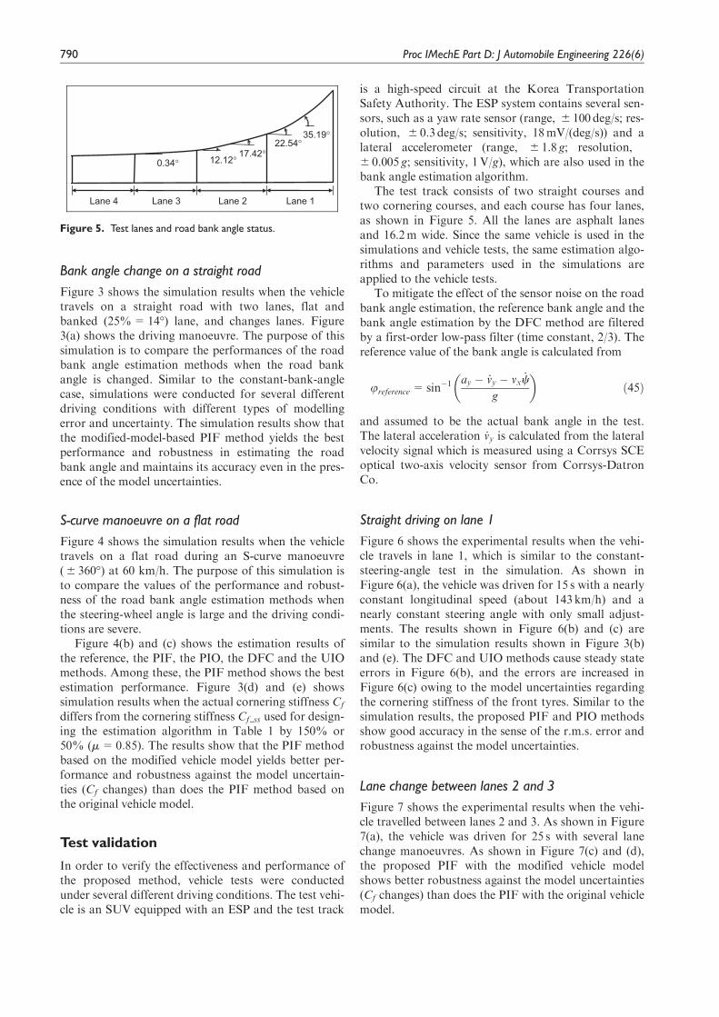
is a high-speed circuit at the Korea TransportationSafety Authority. The ESP system contains several sen-sors, such as a yaw rate sensor (range, 6 100 deg/s; res-olution, 6 0.3 deg/s; sensitivity, 18mV/(deg/s)) and alateral accelerometer (range, 6 1.8 g; resolution,6 0.005 g; sensitivity, 1V/g), which are also used in thebank angle estimation algorithm.

The test track consists of two straight courses andtwo cornering courses, and each course has four lanes,as shown in Figure 5. All the lanes are asphalt lanesand 16.2m wide. Since the same vehicle is used in thesimulations and vehicle tests, the same estimation algo-rithms and parameters used in the simulations areapplied to the vehicle tests.

To mitigate the effect of the sensor noise on the roadbank angle estimation, the reference bank angle and thebank angle estimation by the DFC method are filteredby a first-order low-pass filter (time constant, 2/3). Thereference value of the bank angle is calculated from

ureference=sin�1ay � _vy � vx _c

g

� �ð45Þ

and assumed to be the actual bank angle in the test.The lateral acceleration _vy is calculated from the lateralvelocity signal which is measured using a Corrsys SCEoptical two-axis velocity sensor from Corrsys-DatronCo.

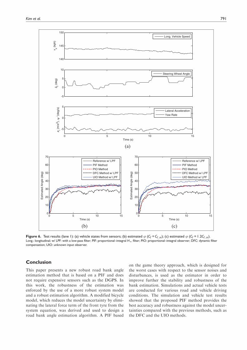
Straight driving on lane 1

Figure 6 shows the experimental results when the vehi-cle travels in lane 1, which is similar to the constant-steering-angle test in the simulation. As shown inFigure 6(a), the vehicle was driven for 15 s with a nearlyconstant longitudinal speed (about 143km/h) and anearly constant steering angle with only small adjust-ments. The results shown in Figure 6(b) and (c) aresimilar to the simulation results shown in Figure 3(b)and (e). The DFC and UIO methods cause steady stateerrors in Figure 6(b), and the errors are increased inFigure 6(c) owing to the model uncertainties regardingthe cornering stiffness of the front tyres. Similar to thesimulation results, the proposed PIF and PIO methodsshow good accuracy in the sense of the r.m.s. error androbustness against the model uncertainties.

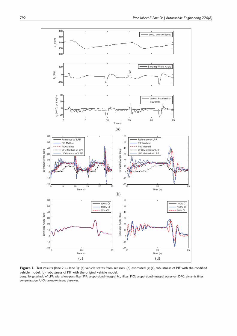
Lane change between lanes 2 and 3

Figure 7 shows the experimental results when the vehi-cle travelled between lanes 2 and 3. As shown in Figure7(a), the vehicle was driven for 25 s with several lanechange manoeuvres. As shown in Figure 7(c) and (d),the proposed PIF with the modified vehicle modelshows better robustness against the model uncertainties(Cf changes) than does the PIF with the original vehiclemodel.

° °°

°°

Figure 5. Test lanes and road bank angle status.


Conclusion

This paper presents a new robust road bank angleestimation method that is based on a PIF and doesnot require expensive sensors such as the DGPS. Inthis work, the robustness of the estimation wasenforced by the use of a more robust system modeland a robust estimation algorithm. A modified bicyclemodel, which reduces the model uncertainty by elimi-nating the lateral force term of the front tyre from thesystem equation, was derived and used to design aroad bank angle estimation algorithm. A PIF based

on the game theory approach, which is designed forthe worst cases with respect to the sensor noises anddisturbances, is used as the estimator in order toimprove further the stability and robustness of thebank estimation. Simulations and actual vehicle testsare conducted for various road and vehicle drivingconditions. The simulation and vehicle test resultsshowed that the proposed PIF method provides thebest accuracy and robustness against the model uncer-tainties compared with the previous methods, such asthe DFC and the UIO methods.

140

145

150

v x (kp

h)

Long. Vehicle Speed

-5

0

5

10

δ f (de

g)


0 5 10 15

-5

0

5

a y (m

/s2 )

, ψ

′(deg

/s)

Time (s)

Lateral Acceleration

Yaw Rate

(a)

0 5 10 150

10

20

30

40

50

60

70

Est

imat

ed A

ngle

(de

g)

Time (s)

Reference w/ LPF

PIF Method

PIO MethodDFC Method w/ LPF

UIO Method w/ LPF

0 5 10 150

10

20

30

40

50

60

70

Est

imat

ed A

ngle

(de

g)

Time (s)

Reference w/ LPF

PIF Method


UIO Method w/ LPF

(b) (c)

Figure 6. Test results (lane 1): (a) vehicle states from sensors; (b) estimated u (Cf = Cf ss); (c) estimated u (Cf = 1:2Cf ss).Long.: longitudinal; w/ LPF: with a low-pass filter; PIF: proportional–integral HN filter; PIO: proportional–integral observer; DFC: dynamic filter

compensation; UIO: unknown input observer.

Kim et al. 791

120

130

140

150

160

vx (

kph)

Long. Vehicle Speed

-100

0

100

δ f (de

g)


0 5 10 15 20 25

-20

0

20

40

ay

(m/s

2 ),

ψ′(d

eg/s

)

Time (s)

Lateral Acceleration

Yaw Rate

(a)

0 5 10 15 20 25-20

-10

0

10

20

30

40

50

60

Est

imat

ed A

ngle

(de

g)

Time (s)

Reference w/ LPF

PIF Method


UIO Method w/ LPF

15 20 25-20

-10

0

10

20

30

40

50

60

Est

imat

ed A

ngle

(de

g)

Time (s)

Reference w/ LPF

PIF Method


UIO Method w/ LPF

(b)

(c) (d)

15 20 25-20

-10

0

10

20

30

40

50

60

Est

imat

ed A

ngle

(de

g)

Time (s)

100% Cf

150% Cf50% Cf

15 20 25-20

-10

0

10

20

30

40

50

60

Est

imat

ed A

ngle

(de

g)

Time (s)

100% Cf

150% Cf50% Cf

Figure 7. Test results (lane 2$ lane 3): (a) vehicle states from sensors; (b) estimated u; (c) robustness of PIF with the modifiedvehicle model; (d) robustness of PIF with the original vehicle model.Long.: longitudinal; w/ LPF: with a low-pass filter; PIF: proportional–integral HN filter; PIO: proportional–integral observer; DFC: dynamic filter

compensation; UIO: unknown input observer.


Funding

This work was supported by Industry SourceFoundation Establishment Project (grant no. 10037355)from the Korea Institute for Advancement ofTechnology, funded by the Ministry of KnowledgeEconomy, Republic of Korea, and the research fund ofHanyang University, Seoul, Republic of Korea.

References

1. Van Zanten AT, Erhardt R and Pfaff G. VDC, the vehicle

dynamic control system of Bosch. SAE paper 950759, 1995.2. Tseng HE, Ashrafi B, Madau D, et al. The development

of vehicle stability control at Ford. IEEE/ASME Trans

Mechatronics 1999; 4(3): 223–234.3. Yoon J, Cho W, Koo B and Yi K. Unified chassis con-

trol for rollover prevention and lateral stability. IEEE

Trans Veh Technol 2009; 58(2): 596–609.4. Park J-I, Yoon J-Y, Kim D-S and Yi K-S. Roll state esti-

mator for rollover mitigation control. Proc IMechE Part

D: J Automobile Engineering 2008; 222(8): 1289–1311.5. Cetin AE, Adli MA, Barkana DE and Kucuk H. Imple-

mentation and development of an adaptive steering-

control system. IEEE Trans Veh Technol 2010; 59(1):

75–83.6. Zheng B and Anwar S. Yaw stability control of a steer-

by-wire equipped vehicle via active front wheel steering.

Mechatronics 2009; 19(6): 799–804.7. Sankaranarayanan V, Emekli ME, Guvenc BA, et al.

Semiactive suspension control of a light commercial

vehicle. IEEE/ASME Trans Mechatronics 2008; 13(5):

598–604.8. Tseng HE. Dynamic estimation of road bank angle. Veh

System Dynamics 2001; 36(4–5): 307–328.9. Piyabongkarn D, Rajamani R, Grogg JA and Lew JY.

Development and experimental evaluation of a slip angle

estimator for vehicle stability control. IEEE Trans Con-

trol Systems Technol 2009; 17(1): 78–88.10. Ryu J and Gerdes JC. Estimation of vehicle roll and road

bank angle. In: 2004 American control conference, Boston,

MA, USA, 30 June–2 July 2004, vol 3, pp. 2110–2115.

New York: IEEE.11. Rajamani R, Piyabongkarn D, Tsourapas V and Lew

JY. Real-time estimation of roll angle and CG height for

active rollover prevention applications. In: 2009 Ameri-

can control conference, St Louis, MO, USA, 10–12 June

2009, pp. 433–438. New York: IEEE.12. Xu L and Tseng HE. Robust model-based fault detection

for a roll stability control system. IEEE Trans Control

Systems Technol 2007; 15(3): 519–528.13. Mammer S, Glaser S and Netto M. Vehicle lateral

dynamics estimation using unknown input proportional-

integral observers. In: 2006 American control conference,

Minneapolis, MN, USA, 14–16 June 2006, pp. 4658–

4663. New York: IEEE.14. Hahn JO, Rajamani R, You SH and Lee KI. Real-time

identification of road bank angle using differential GPS.

IEEE Trans Control Systems Technol 2004; 12: 589–599.15. Luczak S, Oleksiuk W and Bodnicki M. Sensing tilt with

MEMS accelerometers. IEEE Sensors J 2006; 6(6): 1669–

1675.16. Fukada Y. Estimation of vehicle slip-angle with combi-

nation method of model observer and direct integration.

In: 4th international symposium on advanced vehicle con-trol, Nagoya, Japan, 14–18 September 1998, pp. 375–388.Tokyo: JSAE.

17. Nishio A, Tozu K, Yamaguchi H, et al. Development ofvehicle stability control system based on vehicle sideslipangle estimation. SAE paper 2001-01-0137, 2001.

18. Imsland L, Grip HF, Johansen TA and Fossen TI. Onnonlinear unknown input observers – applied to lateralvehicle velocity estimation on banked roads. Int J Control2006; 80(11): 1741–1750.

19. Hsu L-Y and Chen T-L. Estimating road angles with theknowledge of the vehicle yaw angle. Trans ASME, JDynamic Systems, Measmt, Control 2010; 132(3): 31004.

20. Sebsadji Y, Glaser S and Mammar S. Vehicle roll androad bank angles estimation. In: 17th IFAC world con-gress, Seoul, Republic of Korea, 6–11 July 2008, pp.7091–7097. Oxford: Elsevier.

21. Grip HF, Imsland L, Johansen TA, et al. Estimation ofroad inclination and bank angle in automotive vehicles.In: 2009 American control conference, St Louis, MO,USA, 10–12 June 2009, pp. 426–432. New York: IEEE.

22. Rajamani R. Vehicle dynamics and control. New York:Springer, 2005.

23. Jazar RN. Vehicle dynamics: theory and applications. NewYork: Springer, 2008.

24. Chen J and Patton RJ. Robust model-based fault diagnosisfor dynamic systems. Norwell, MA: Kluwer, 1999.

25. Soffker D, Yu TJ and Muller PC. State estimation ofdynamical systems with nonlinearities by usingproportional–integral observer. Int J Systems Sci 1995;26(9): 1571–1582.

26. Jiang G-P, Wang S-P and Song W-Z. Design of observerwith integrators for linear systems with unknown inputdisturbances. Electron Lett 2000; 36(13): 1168–1169.

27. Marek J, Trah H-P, Suzuki Y and Yokomori I. Sensorsfor automotive technology. Weinheim: Wiley–VCH, 2003.

28. Banavar RN and Speyer JL. A linear-quadratic gameapproach to estimation and smoothing. In: American con-trol conference, Boston, MA, USA, 26–28 June 1991, pp.2818–2822. New York: IEEE.

29. de Souza CE, Shaked U and Fu M. Robust H‘ filteringfor continuous time varying uncertain systems with deter-ministic input signals. IEEE Trans Signal Processing1995; 43(3): 709-719.

30. Simon D. Optimal state estimation: Kalman, HN, and non-linear approaches.Hoboken, NJ: John Wiley, 2006.

31. Burl JB. Linear optimal control. Reading, MA: AddisonWesley Longman, 1999.

32. Kamnik R, Boettiger F and Hunt K. Roll dynamics andlateral load transfer estimation in articulated heavyfreight vehicles: a simulation study. Proc IMechE Part D:J Automobile Engineering 2003; 217(11): 985–997.

Appendix

Notation

ay lateral acceleration of the vehicle (m/s2)A state matrixAm state matrix for the modified bicycle

modelAo state matrix for the original bicycle modelAw state matrix for the bicycle model based

on the proportional–integral observer

Kim et al. 793

B input matrixC output matrixCf cornering stiffness of the front tyres

(N/rad)Cr cornering stiffness of the rear tyres

(N/rad)D input-to-output coupling matrixe estimation errorE input matrix for the disturbance inputFyf front lateral force (N)Fyr rear lateral force (N)g acceleration due to gravityG transfer function matrixh distance from the centre of gravity to the

roll centre (m)H transfer functionI identity matrixIz yaw moment of inertia of the vehicle

(kg m2)J cost functionK gain matrixKus understeer gradient of the vehicleL observer output matrixLf distance from the front axle to the centre

of gravity (m)Lr distance from the rear axle to the centre of

gravity (m)m mass of the vehicle (kg)M weight matrix for the outputsn disturbance input for the bicycle model

based on the proportional–integral observer

P Riccati solutionQ weight matrix for the disturbancesR weight matrix for the noisess Laplace variableS weight matrix for the estimation errorst time (s)tf final time (s)u system inputv measurement noisevx longitudinal speed of the vehicle (m/s)vy lateral speed of the vehicle (m/s)w disturbance inputx system statex estimate of xxð0Þ initial stateX(s) Laplace transform of xy system outputz transformed state

af front-tyre side-slip angle (rad)ar rear-tyre side-slip angle (rad)b vehicle side-slip angle (rad)bf global front-tyre sideslip angle (rad)br global rear-tyre sideslip angle (rad)df steering-wheel angle (rad)u parameter for the cost functionm tyre–road friction coefficientf roll angle of the vehicle (rad)fb road bank angle (rad)c yaw angle of the vehicle (rad)


proc imeche part d: a robust road bank angle estimation ...acl.kaist.ac.kr/thesis/2012_jae.pdf ·...

Documents