1 INTRODUCTION

Submarine landslides occur below water level, and our knowledge of their development is rather limited (Andresen & Bjerrum 1967). These submarine land-slides are rather mysterious, as they frequently occur in slopes that should be stable beyond any doubt ac-cording to a conventional stability analysis. Most importantly they have significant impacts and con-sequences on offshore and coastal facilities such as oil and gas production wells, platforms, pipelines, seafloor communication cables, marine habitats, leading to considerable damages to properties and loss of lives. It is therefore the knowledge and fur-ther understanding of submarine landslides is essen-tial to mitigate these occurrences. A number of laboratory experimental works has been carried out by other researchers to investigate the mechanisms of long run-out submarine land-slides and submarine debris flows (Mohrig et al. 1998; Mohrig, et al. 1999; Mohrig, et al. 2003; Ilstad et al. 2004a,b,c; Ilstad 2005). However, all these ex-perimental works were performed in 1 g test envi-ronment. It should be noted that the actual subma-rine slides are very large while the scaled model in 1 g test environment is relatively small, hence the soil stresses in such condition is also small and may not represent the real situations.

With centrifuge modelling, self weight stresses and gravity dependent processes are able to be cor-rectly reproduced and observations from small scale models can be related to the full scale prototype situation using appropriate scaling laws. This paper discusses the data from a series of centrifuge tests and the scaling laws for submarine landslide flows in centrifuge testing. 2 EXPERIMENTAL DETAILS & PROCEDURES

2.1 Centrifuge apparatus

The mini-drum centrifuge at the University of Cam-bridge is specifically chosen for the submarine land-slide flows experiments because of its flexibility for materials to move freely within the circular channel. Unlike beam centrifuges, the soil test package is mounted on one end of the rotating arm.

The mini-drum centrifuge has a radius of 370 mm with a width of 180 mm and depth of 120 mm. Ac-cording to Barker (1998), the maximum speed of the motor in the mini-drum centrifuge is 1067 rpm which corresponds to 471 times earth’s gravity at radius 370 mm.

Centrifuge modelling of submarine landslide flows

C.S. Gue University of Cambridge, Cambridge, United Kingdom

Norwegian Geotechnical Institute, Oslo, Norway

International Centre for Geohazards, Oslo, Norway

K. Soga & M. Bolton University of Cambridge, Cambridge, United Kingdom

N.I. Thusyanthan KW Ltd, Surrey, United Kingdom

ABSTRACT: Landslides occur both onshore and offshore, however rather little attention has been given to offshore landslides (submarine landslides). Although land and submarine landslides have many similarities in terms of landslide mechanics, some unique characteristics of submarine landslides include large mass move-ments and long travel distances at very gentle slopes. These submarine landslides have significant impacts and consequences on offshore and coastal facilities such as oil and gas production wells, platforms, pipelines and seafloor communication cables. This paper presents data from a series of centrifuge tests in which simula-tions of submarine landslide flows on a very gentle slope were conducted. Experiments were conducted at dif-ferent gravity levels to understand the scaling laws involved in simulation of submarine landslide flows in centrifuge testing. The slope was instrumented with miniature sensors for measurements of pore pressure and soil stresses beneath the submarine landslide flow. A series of digital cameras were used to capture the land-slide flow in flight. The results provide a better understanding of the scaling laws that needs to be adopted for centrifuge experiments involving submarine landslide flows. Hence, the results from the experiments also give an insight into the flow mechanism involved in submarine landslide flows.

Proc 7th International Conference on Physical Modelling in Geotechnics, Zurich, 2, 1113-1118

0.13

Side view of the instrumentation

0.5

77.40

0.5

PPT

Slope

Plan view of the instrumentationAluminium plate

PPTs and Stress Cells

Circular foam slope

0.17

0.19

0.21

Head tank

Opening atHead tank

0.17 0.19 0.210.096

0.09

2

0.0

2 0.0

98

Stress Cell1.00

0.105

Perspex windowsunits in m

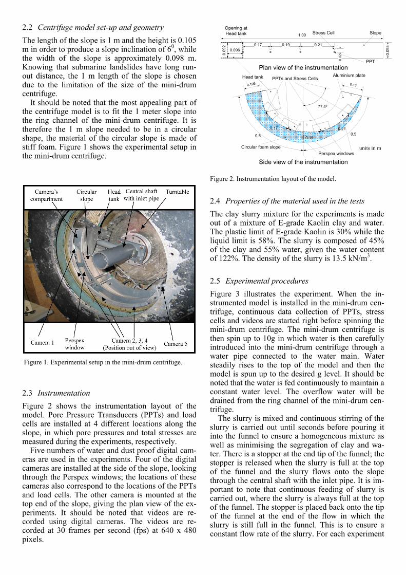
2.2 Centrifuge model set-up and geometry

The length of the slope is 1 m and the height is 0.105 m in order to produce a slope inclination of 60, while the width of the slope is approximately 0.098 m. Knowing that submarine landslides have long run-out distance, the 1 m length of the slope is chosen due to the limitation of the size of the mini-drum centrifuge.

It should be noted that the most appealing part of the centrifuge model is to fit the 1 meter slope into the ring channel of the mini-drum centrifuge. It is therefore the 1 m slope needed to be in a circular shape, the material of the circular slope is made of stiff foam. Figure 1 shows the experimental setup in the mini-drum centrifuge.

Figure 1. Experimental setup in the mini-drum centrifuge.

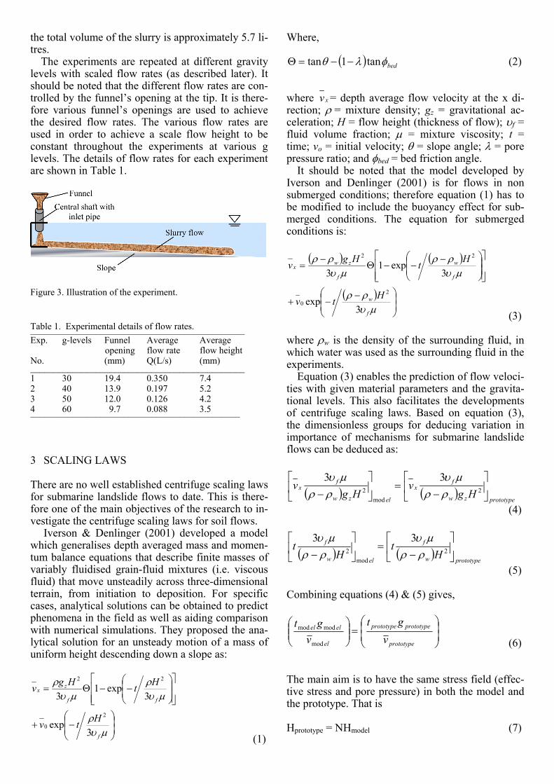
2.3 Instrumentation

Figure 2 shows the instrumentation layout of the model. Pore Pressure Transducers (PPTs) and load cells are installed at 4 different locations along the slope, in which pore pressures and total stresses are measured during the experiments, respectively.

Five numbers of water and dust proof digital cam-eras are used in the experiments. Four of the digital cameras are installed at the side of the slope, looking through the Perspex windows; the locations of these cameras also correspond to the locations of the PPTs and load cells. The other camera is mounted at the top end of the slope, giving the plan view of the ex-periments. It should be noted that videos are re-corded using digital cameras. The videos are re-corded at 30 frames per second (fps) at 640 x 480 pixels.

Figure 2. Instrumentation layout of the model.

2.4 Properties of the material used in the tests

The clay slurry mixture for the experiments is made out of a mixture of E-grade Kaolin clay and water. The plastic limit of E-grade Kaolin is 30% while the liquid limit is 58%. The slurry is composed of 45% of the clay and 55% water, given the water content of 122%. The density of the slurry is 13.5 kN/m3.

2.5 Experimental procedures

Figure 3 illustrates the experiment. When the in-strumented model is installed in the mini-drum cen-trifuge, continuous data collection of PPTs, stress cells and videos are started right before spinning the mini-drum centrifuge. The mini-drum centrifuge is then spin up to 10g in which water is then carefully introduced into the mini-drum centrifuge through a water pipe connected to the water main. Water steadily rises to the top of the model and then the model is spun up to the desired g level. It should be noted that the water is fed continuously to maintain a constant water level. The overflow water will be drained from the ring channel of the mini-drum cen-trifuge.

The slurry is mixed and continuous stirring of the slurry is carried out until seconds before pouring it into the funnel to ensure a homogeneous mixture as well as minimising the segregation of clay and wa-ter. There is a stopper at the end tip of the funnel; the stopper is released when the slurry is full at the top of the funnel and the slurry flows onto the slope through the central shaft with the inlet pipe. It is im-portant to note that continuous feeding of slurry is carried out, where the slurry is always full at the top of the funnel. The stopper is placed back onto the tip of the funnel at the end of the flow in which the slurry is still full in the funnel. This is to ensure a constant flow rate of the slurry. For each experiment

the total volume of the slurry is approximately 5.7 li-tres.

The experiments are repeated at different gravity levels with scaled flow rates (as described later). It should be noted that the different flow rates are con-trolled by the funnel’s opening at the tip. It is there-fore various funnel’s openings are used to achieve the desired flow rates. The various flow rates are used in order to achieve a scale flow height to be constant throughout the experiments at various g levels. The details of flow rates for each experiment are shown in Table 1.

Figure 3. Illustration of the experiment. Table 1. Experimental details of flow rates. ______________________________________________ Exp. g-levels Funnel Average Average opening flow rate flow height No. (mm) Q(L/s) (mm) ______________________________________________ 1 30 19.4 0.350 7.4 2 40 13.9 0.197 5.2 3 50 12.0 0.126 4.2 4 60 09.7 0.088 3.5 _____________________________________________ 3 SCALING LAWS

There are no well established centrifuge scaling laws for submarine landslide flows to date. This is there-fore one of the main objectives of the research to in-vestigate the centrifuge scaling laws for soil flows.

Iverson & Denlinger (2001) developed a model which generalises depth averaged mass and momen-tum balance equations that describe finite masses of variably fluidised grain-fluid mixtures (i.e. viscous fluid) that move unsteadily across three-dimensional terrain, from initiation to deposition. For specific cases, analytical solutions can be obtained to predict phenomena in the field as well as aiding comparison with numerical simulations. They proposed the ana-lytical solution for an unsteady motion of a mass of uniform height descending down a slope as:

f

ff

zx

Htv

Ht

Hgv

3exp

3exp1

3

2

0

22

(1)

Where,

bed tan1tan (2) where xv = depth average flow velocity at the x di-rection; = mixture density; gz = gravitational ac-celeration; H = flow height (thickness of flow); f = fluid volume fraction; = mixture viscosity; t = time; vo = initial velocity; = slope angle; = pore pressure ratio; and bed = bed friction angle. It should be noted that the model developed by Iverson and Denlinger (2001) is for flows in non submerged conditions; therefore equation (1) has to be modified to include the buoyancy effect for sub-merged conditions. The equation for submerged conditions is:

f

w

f

w

f

zwx

Htv

Ht

Hgv

3exp

3exp1

3

2

0

22

(3)

where w is the density of the surrounding fluid, in which water was used as the surrounding fluid in the experiments. Equation (3) enables the prediction of flow veloci-ties with given material parameters and the gravita-tional levels. This also facilitates the developments of centrifuge scaling laws. Based on equation (3), the dimensionless groups for deducing variation in importance of mechanisms for submarine landslide flows can be deduced as:

prototypezw

fx

elzw

fx

Hgv

Hgv

2

mod

2

33

(4)

prototypew

f

elw

f

Ht

Ht

2

mod

2

33

(5) Combining equations (4) & (5) gives,

prototype

prototypeprototype

el

elel

v

gt

v

gt

mod

modmod (6)

The main aim is to have the same stress field (effec-tive stress and pore pressure) in both the model and the prototype. That is Hprototype = NHmodel (7)

0 2 4 6 8 10 12-20246

0 2 4 6 8 10 12-20246

0 2 4 6 8 10 12-20246

0 2 4 6 8 10 12-20246

Time (s)

Cha

nge

in P

ore

Pre

ssur

e (

kPa)

30g40g50g60g

PPT 2 (0.17 m from opening of head tank)

PPT 3 (0.36 m from opening of head tank)

PPT 4 (0.57 m from opening of head tank)

PPT 1 (0 m from opening of head tank)

Based on equation (3) and the dimensionless groups, the scaling laws for submarine landslide flows of viscous soil-water mixture can be deduced as: Vprototype = NVmodel (8) tprototype = N2tmodel (9) Lprototype = N3Lmodel (10) where H = flow height; V = flow velocity; t = time; and L = flow distance (run-out). It is intriguing to find out that the flow distance of a prototype will scaled at N3 times of the model. Based on the conventional centrifuge scaling law of soil body, the horizontal movement would have scaled at N times of the model. This has further mo-tivated the call for carrying out the centrifuge ex-periments to validate the deduced scaling laws. It should be noted that the injected slurry flow rates shown in Table 1 are scaled in order to give the scaled flow height to be the same for the appropriate g levels (eq.7), in which the validity of equation (8, 9 & 10) are checked. The prototype flow height is approximately 0.21 m. Ideally this will give the same magnitude of basal friction to resist the flow movement as well as soil stress field to drive the soil body to move along the slope. 4 RESULTS

Figure 4 shows the change in pore pressure meas-ured at various locations and g levels beneath the submarine landslide flows along the slope. The change in pore pressure at different g levels is rela-tively comparable. This means that the stresses at various g levels are possibly correctly modelled. The change in pore pressure generally increases when the front of the flow arrives at the location of the PPTs. Figure 5 shows the side view of the submarine landslide flow at the opening of the head tank, pic-ture frames extracted from the digital videos (from Camera 1, refer Figure 1). The interval of these pic-tures is at 0.033s based on the 30fps video frame rate of the digital camera.

In order to check the scaling law for the flow dis-tance, the flow distance with time has to be extracted based on the camera that is mounted at the top end of the slope. It gives the plan view of the submarine landslide flow (Camera 5, refer Figure 1). It should be noted that the picture frame from the plan view provides the view of a longer flow distance as com-pared to the picture frame from the side views. Fig-ure 6 shows the sequence of the submarine landslide flow from the plan view. The interval of these pic-tures is at 0.033s. For the ease of extracting the flow distance from each picture frames, Photoshop is

used to combine these picture frames as shown in Figure 7.

Figure 8 shows the normalised flow distance

against the normalised time at various g levels. The normalisation is based on the proposed scaling laws, where the flow distance is scaled at N3 times of the model and the time is scaled at N2 times of the model. It can be seen that the experimental data from various g levels scale reasonably well to the proposed scaling laws.

Figure 4. The change in pore pressure at various locations along the slope.

Figure 5. Side view of the submarine landslide flow at the opening of the head tank (picture interval at 0.033s).

(a) (b)

(d)(c)

(f)(e)

1 cm

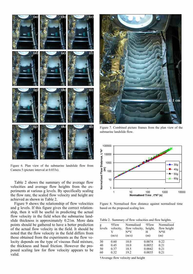
Figure 6. Plan view of the submarine landslide flow from Camera 5 (picture interval at 0.033s).

Table 2 shows the summary of the average flow

velocities and average flow heights from the ex-periments at various g levels. By specifically scaling the flow rate, the scaled flow velocity and height are achieved as shown in Table 2.

Figure 9 shows the relationship of flow velocities and g levels. If this figure gives the correct relation-ship, then it will be useful in predicting the actual flow velocity in the field when the submarine land-slide thickness is approximately 0.21m. More data points should be gathered to have a better prediction of the actual flow velocity in the field. It should be noted that the flow velocity in the field differs from those obtained from the experiments as the flow ve-locity depends on the type of viscous fluid mixture, the thickness and basal friction. However the pro-posed scaling law for flow velocity appears to be valid.

Figure 7. Combined picture frames from the plan view of the submarine landslide flow.

Figure 8. Normalised flow distance against normalised time based on the proposed scaling law.

Table 2. Summary of flow velocities and flow heights. ______________________________________________ g †Flow Normalised †Flow Normalised levels velocity, flow velocity, height, flow height V N*V H N*H

(m/s) (m/s) (m) (m) ______________________________________________ 30 0.60 18.0 0.0074 0.22 40 0.45 18.0 0.0052 0.21 50 0.37 18.5 0.0042 0.21 60 0.32 19.2 0.0035 0.21 _____________________________________________ †Average flow velocity and height

(a) (b) (c)

(d) (e) (f)

(g) (h) (i)

(j) (k) (l)

1 cm

30g

40g

50g

60g

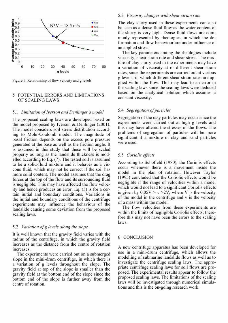
Figure 9. Relationship of flow velocity and g levels.

5 POTENTIAL ERRORS AND LIMITATIONS OF SCALING LAWS

5.1 Limitation of Iverson and Denlinger’s model

The proposed scaling laws are developed based on the model proposed by Iverson & Denlinger (2001). The model considers soil stress distribution accord-ing to Mohr-Coulomb model. The magnitude of basal friction depends on the excess pore pressure generated at the base as well as the friction angle. It is assumed in this study that these will be scaled properly as long as the landslide thickness is mod-elled according to Eq. (7). The tested soil is assumed to be a solid-fluid mixture and it behaves as a vis-cous fluid, which may not be correct if the soil has more solid content. The model assumes that the drag forces at the top of the flow and its surrounding fluid is negligible. This may have affected the flow veloc-ity and hence produces an error. Eq. (3) is for a cer-tain initial and boundary conditions. Variations in the initial and boundary conditions of the centrifuge experiments may influence the behaviour of the landslide causing some deviation from the proposed scaling laws.

5.2 Variation of g levels along the slope

It is well known that the gravity field varies with the radius of the centrifuge, in which the gravity field increases as the distance from the centre of rotation increases.

The experiments were carried out on a submerged slope in the mini-drum centrifuge, in which there is a variation of g levels throughout the slope. The gravity field at top of the slope is smaller than the gravity field at the bottom end of the slope since the bottom end of the slope is further away from the centre of rotation.

5.3 Viscosity changes with shear strain rate

The clay slurry used in these experiments can also be seen as a dense fluid flow as the water content of the slurry is very high. Dense fluid flows are com-monly represented by rheologies, in which the de-formation and flow behaviour are under influence of an applied stress. The key parameters among the rheologies include viscosity, shear strain rate and shear stress. The mix-ture of clay slurry used in the experiments may have a variation of viscosity at or different shear strain rates, since the experiments are carried out at various g levels, in which different shear strain rates are ap-plied within the flow. This may lead to an error in the scaling laws since the scaling laws were deduced based on the analytical solution which assumes a constant viscosity.

5.4 Segregation of particles

Segregation of the clay particles may occur since the experiments were carried out at high g levels and this may have altered the stresses of the flows. The problems of segregation of particles will be more significant if a mixture of clay and sand particles were used.

5.5 Coriolis effects

According to Schofield (1980), the Coriolis effects occur whenever there is a movement inside the model in the plan of rotation. However Taylor (1995) concluded that the Coriolis effects would be negligible if the range of velocities within a model which would not lead to a significant Coriolis effects is given by 0.05V > >2V, where V is the velocity of the model in the centrifuge and is the velocity of a mass within the model. The flow velocities from these experiments are within the limits of negligible Coriolis effects; there-fore this may not have been the errors to the scaling laws.

6 CONCLUSION

A new centrifuge apparatus has been developed for use in a mini-drum centrifuge, which allows the modelling of submarine landslide flows as well as to investigate the centrifuge scaling laws. The appro-priate centrifuge scaling laws for soil flows are pro-posed. The experimental results appear to follow the proposed scaling laws. The limitations of the scaling laws will be investigated through numerical simula-tions and this is the on-going research work.

N*V = 18.5 m/s

00.10.20.30.40.50.60.70.80.9

1

0 10 20 30 40 50 60 70 80

g levels

Ave

rag

e f

low

vel

oc

ity

(m/s

)

30g

40g

50g

60g

ACKNOWLEDGEMENTS

The present study is funded by the Norwegian Geo-technical Institute, International Centre for Geohaz-ards and the Cambridge Commonwealth Trust.

The assistance of the laboratory technicians at the Schofield Centre, Engineering Department of the University of Cambridge is also acknowledged. REFERENCES

Andresen, A. & Bjerrum, L. 1967. Slides in subaqueous slopes in loose sand and silt. In Adrain F. Richards (ed.), Marine Geotechnique,University of Illinois Press: 221-239.

Baker, H.R. 1998. Physical Modelling of Construction Processes in the Mini-Drum Centrifuge. PhD Thesis, University of Cambridge.

Ilstad, T. 2005. On the Dynamics and Morphology of Submarine Debris Flows. PhD thesis. University of Oslo.

Ilstad, T., De Blasio, F.V., Elverhøi, A., Harbitz, C.B., Engvik, L., Longva, O., & Marr, J.G. 2004c. On the frontal dynamics and morphology of submarine debris flows. Marine Geology, 213: 481-497.

Ilstad, T. Elverhøi, A., Issler, D., & Marr, J.G. 2004b. Subaqueous debris flow behaviour and its dependence on the sand/clay ratio: a laboratory study using particle tracking. Marine Geology, 213: 415-438.

Ilstad, T., Marr, J.G., Elverhøi, A., & Harbitz, C.B. 2004a. Laboratory studies of subaqueous debris flows by measurements of pore-fluid pressure and total stress. Marine Geology, 213: 403-414.

Iverson, R.M. & Denlinger, R.P. 2001. Flow of variably fluidized granular masses across three-dimensional terrain – 1. Coulomb mixture theory. Journal of Geophysical Research, Vol. 106, No. B1: 537-552.

Mohrig, D., Elverhøi, A., & Parker, G. 1999. Experiments on the relative mobility of muddy subaqueous and subaerial debris flows, and their capacity to remobilise antecedent deposits. Marine Geology, 154: 117-129.

Mohrig, D., & Marr, J.G. 2003. Constraining the efficiency of turbidity current generation from submarine debris flows and slides using laboratory experiments. Marine and Petroleum Geology, 20: 883-899.

Mohrig, D., Whipple, K.X., Hondzo, M., Ellis, C., & Parker, G.Jappelli, R. & Marconi, N. 1998. Hydroplaning of subaqueous debris flows. Geological Society of America Bulletin, March, Vol. 110, No.3: 387-394.

Schofield, A.N. 1980. Cambridge geotechnical centrifuge op-erations. Geotechnique, 30: 227-268.

Taylor, R.N. 1995 (ed.). Geotechnical Centrifuge Technology. London: Blackie Academic & Professional.