problem solving and search - chapter 3
TRANSCRIPT

Problem solving and searchChapter 3
Artificial Intelligence
Slides from AIMA — http://aima.cs.berkeley.edu
1 / 50
Outline
I Problem-solving agentsI Problem typesI Problem formulationI Example problemsI Basic search algorithmsI Informed search algorithms
2 / 50

Problem-solving agents
Restricted form of general agent:
function Simple-Problem-Solving-Agent( percept) returns an actionstatic: seq, an action sequence, initially empty
state, some description of the current world stategoal, a goal, initially nullproblem, a problem formulation
state←Update-State(state, percept)if seq is empty then
goal←Formulate-Goal(state)problem←Formulate-Problem(state, goal)seq←Search( problem)
action←Recommendation(seq, state)seq←Remainder(seq, state)return action
Note: this is offline problem solving; solution executed “eyes closed.”Online problem solving involves acting without complete knowledge.
3 / 50

Example: Romania
On holiday in Romania; currently in Arad.Flight leaves tomorrow from Bucharest
I Formulate goal: be in BucharestI states: various citiesI actions: drive between citiesI Find solution: sequence of cities, e.g., Arad, Sibiu, Fagaras, Bucharest
4 / 50

Example: Romania
Giurgiu
UrziceniHirsova
Eforie
Neamt
Oradea
Zerind
Arad
Timisoara
Lugoj
Mehadia
DobretaCraiova
Sibiu Fagaras
Pitesti
Vaslui
Iasi
Rimnicu Vilcea
Bucharest
71
75
118
111
70
75
120
151
140
99
80
97
101
211
138
146 85
90
98
142
92
87
86
5 / 50

Problem types
I Deterministic, fully observable =⇒ single-state problemI Agent knows exactly which state it will be in; solution is a sequence
I Non-observable =⇒ conformant problemI Agent may have no idea where it is; solution (if any) is a sequence
I Nondeterministic and/or partially observable =⇒ contingency problemI percepts provide new information about current stateI solution is a contingent plan or a policyI often interleave search, execution
I Unknown state space =⇒ exploration problem (“online”)
6 / 50

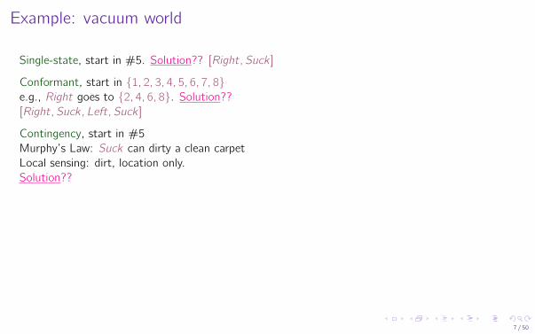
Example: vacuum world
Single-state, start in #5. Solution??
7 / 50

Example: vacuum world
Single-state, start in #5. Solution?? [Right,Suck ]
Conformant, start in {1, 2, 3, 4, 5, 6, 7, 8}e.g., Right goes to {2, 4, 6, 8}. Solution??
7 / 50
Example: vacuum world
Single-state, start in #5. Solution?? [Right,Suck ]
Conformant, start in {1, 2, 3, 4, 5, 6, 7, 8}e.g., Right goes to {2, 4, 6, 8}. Solution??[Right,Suck ,Left,Suck ]
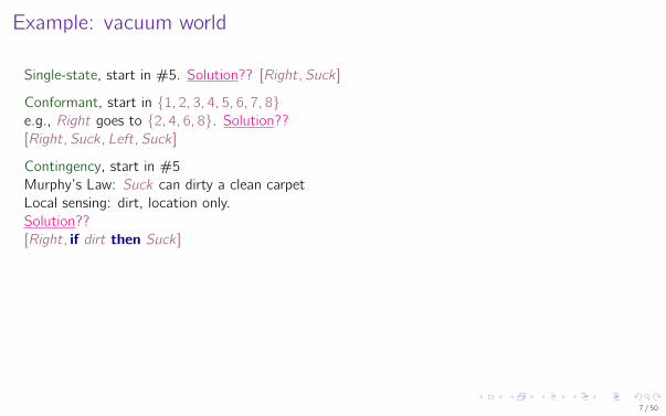
Contingency, start in #5Murphy’s Law: Suck can dirty a clean carpetLocal sensing: dirt, location only.Solution??
7 / 50
Example: vacuum world
Single-state, start in #5. Solution?? [Right,Suck ]
Conformant, start in {1, 2, 3, 4, 5, 6, 7, 8}e.g., Right goes to {2, 4, 6, 8}. Solution??[Right,Suck ,Left,Suck ]
Contingency, start in #5Murphy’s Law: Suck can dirty a clean carpetLocal sensing: dirt, location only.Solution??[Right, if dirt then Suck ]
7 / 50

Single-state problem formulation
A problem is defined by four items:
I initial state e.g., “at Arad”I successor function S(x) = set of action–state pairs
e.g., S(Arad) = {〈Arad → Zerind ,Zerind〉, . . .}I goal test, can be
I explicit, e.g., x = “at Bucharest”I implicit, e.g., NoDirt(x)
I path cost (additive) e.g., sum of distances, number of actions executed, etc. c(x , a, y) is thestep cost, assumed to be ≥ 0
A solution is a sequence of actions leading from the initial state to a goal state
8 / 50

Selecting a state space
Real world is absurdly complex⇒ state space must be abstracted for problem solving
I (Abstract) state = set of real statesI (Abstract) action = complex combination of real actions
e.g., “Arad → Zerind” represents a complex set of possible routes, detours, rest stops, etc.For guaranteed realizability, any real state “in Arad” must get to some real state “in Zerind”
I (Abstract) solution = set of real paths that are solutions in the real world
Each abstract action should be “easier” than the original problem!
9 / 50

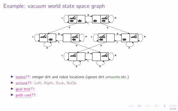
Example: vacuum world state space graphR
L
S S
S S
R
L
R
L
R
L
S
SS
S
L
L
LL R
R
R
R
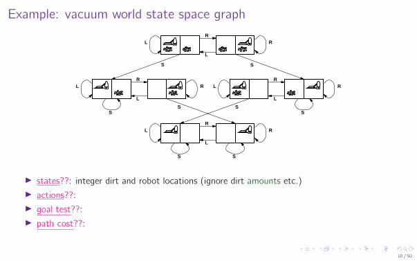
I states??:I actions??:I goal test??:I path cost??:
10 / 50
Example: vacuum world state space graphR
L
S S
S S
R
L
R
L
R
L
S
SS
S
L
L
LL R
R
R
R
I states??: integer dirt and robot locations (ignore dirt amounts etc.)I actions??:I goal test??:I path cost??:
10 / 50
Example: vacuum world state space graphR
L
S S
S S
R
L
R
L
R
L
S
SS
S
L
L
LL R
R
R
R
I states??: integer dirt and robot locations (ignore dirt amounts etc.)I actions??: Left, Right, Suck , NoOpI goal test??:I path cost??:
10 / 50

Example: vacuum world state space graphR
L
S S
S S
R
L
R
L
R
L
S
SS
S
L
L
LL R
R
R
R
I states??: integer dirt and robot locations (ignore dirt amounts etc.)I actions??: Left, Right, Suck , NoOpI goal test??: no dirtI path cost??:
10 / 50

Example: vacuum world state space graphR
L
S S
S S
R
L
R
L
R
L
S
SS
S
L
L
LL R
R
R
R
I states??: integer dirt and robot locations (ignore dirt amounts etc.)I actions??: Left, Right, Suck , NoOpI goal test??: no dirtI path cost??: 1 per action (0 for NoOp)
10 / 50
Example: The 8-puzzle
2
Start State Goal State
51 3
4 6
7 8
5
1
2
3
4
6
7
8
5
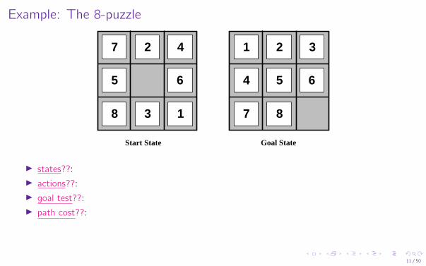
I states??:I actions??:I goal test??:I path cost??:
[Note: optimal solution of n-Puzzle family is NP-hard]
11 / 50

Example: The 8-puzzle
2
Start State Goal State
51 3
4 6
7 8
5
1
2
3
4
6
7
8
5
I states??: integer locations of tiles (ignore intermediate positions)I actions??:I goal test??:I path cost??:
[Note: optimal solution of n-Puzzle family is NP-hard]
11 / 50
Example: The 8-puzzle
2
Start State Goal State
51 3
4 6
7 8
5
1
2
3
4
6
7
8
5
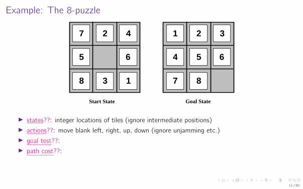
I states??: integer locations of tiles (ignore intermediate positions)I actions??: move blank left, right, up, down (ignore unjamming etc.)I goal test??:I path cost??:
[Note: optimal solution of n-Puzzle family is NP-hard]
11 / 50
Example: The 8-puzzle
2
Start State Goal State
51 3
4 6
7 8
5
1
2
3
4
6
7
8
5
I states??: integer locations of tiles (ignore intermediate positions)I actions??: move blank left, right, up, down (ignore unjamming etc.)I goal test??: = goal state (given)I path cost??:
[Note: optimal solution of n-Puzzle family is NP-hard]
11 / 50

Example: The 8-puzzle
2
Start State Goal State
51 3
4 6
7 8
5
1
2
3
4
6
7
8
5
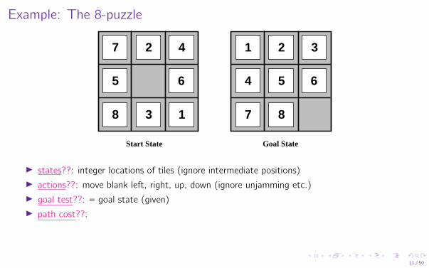
I states??: integer locations of tiles (ignore intermediate positions)I actions??: move blank left, right, up, down (ignore unjamming etc.)I goal test??: = goal state (given)I path cost??: 1 per move
[Note: optimal solution of n-Puzzle family is NP-hard]
11 / 50
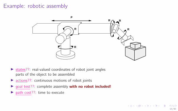
Example: robotic assembly
R
RRP
R R
I states??: real-valued coordinates of robot joint anglesparts of the object to be assembled
I actions??: continuous motions of robot jointsI goal test??: complete assembly with no robot included!I path cost??: time to execute
12 / 50

Tree search algorithms
Basic idea: offline, simulated exploration of state space by generating successors ofalready-explored states (a.k.a. expanding states)
function Tree-Search( problem, strategy) returns a solution, or failureinitialize the search tree using the initial state of problemloop do
if there are no candidates for expansion then return failurechoose a leaf node for expansion according to strategyif the node contains a goal state then return the corresponding solutionelse expand the node and add the resulting nodes to the search tree
end
13 / 50

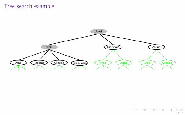
Tree search example
Rimnicu Vilcea Lugoj
ZerindSibiu
Arad Fagaras Oradea
Timisoara
AradArad Oradea
Arad
14 / 50

Tree search example
Rimnicu Vilcea LugojArad Fagaras Oradea AradArad Oradea
Zerind
Arad
Sibiu Timisoara
14 / 50
Tree search example
Lugoj AradArad OradeaRimnicu Vilcea
Zerind
Arad
Sibiu
Arad Fagaras Oradea
Timisoara
14 / 50

Implementation: states vs. nodesI A state is a (representation of) a physical configurationI A node is a data structure constituting part of a search tree
includes parent, children, depth, path cost g(x)
States do not have parents, children, depth, or path cost!
1
23
45
6
7
81
23
45
6
7
8
State Nodedepth = 6
g = 6
state
parent, action
The Expand function creates new nodes, filling in the various fields and using the SuccessorFn ofthe problem to create the corresponding states
15 / 50
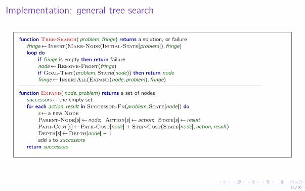
Implementation: general tree search
function Tree-Search( problem, fringe) returns a solution, or failurefringe← Insert(Make-Node(Initial-State[problem]), fringe)loop do
if fringe is empty then return failurenode←Remove-Front(fringe)if Goal-Test(problem,State(node)) then return nodefringe← InsertAll(Expand(node, problem), fringe)
function Expand( node, problem) returns a set of nodessuccessors← the empty setfor each action, result in Successor-Fn(problem,State[node]) do
s← a new NodeParent-Node[s]← node; Action[s]← action; State[s]← resultPath-Cost[s]←Path-Cost[node] + Step-Cost(State[node], action, result)Depth[s]←Depth[node] + 1add s to successors
return successors
16 / 50

Search strategies
A strategy is defined by picking the order of node expansion
Strategies are evaluated along the following dimensions:
completeness: does it always find a solution if one exists?
time complexity: number of nodes generated/expanded
space complexity: maximum number of nodes in memory
optimality: does it always find a least-cost solution?
Time and space complexity are measured in terms of
b : maximum branching factor of the search tree
d : depth of the least-cost solution
m : maximum depth of the state space (may be ∞)
17 / 50

Uninformed search strategies
Uninformed strategies use only the information available in the problem definition
I Breadth-first searchI Uniform-cost searchI Depth-first searchI Depth-limited searchI Iterative deepening search
18 / 50

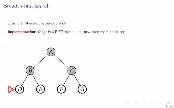
Breadth-first search
Expand shallowest unexpanded node
Implementation: fringe is a FIFO queue, i.e., new successors go at end
A
B C
D E F G
19 / 50

Breadth-first search
Expand shallowest unexpanded node
Implementation: fringe is a FIFO queue, i.e., new successors go at end
A
B C
D E F G
19 / 50

Breadth-first search
Expand shallowest unexpanded node
Implementation: fringe is a FIFO queue, i.e., new successors go at end
A
B C
D E F G
19 / 50
Breadth-first search
Expand shallowest unexpanded node
Implementation: fringe is a FIFO queue, i.e., new successors go at end
A
B C
D E F G
19 / 50

Properties of breadth-first search
I Complete??
I Time??I Space??I Optimal??
20 / 50

Properties of breadth-first search
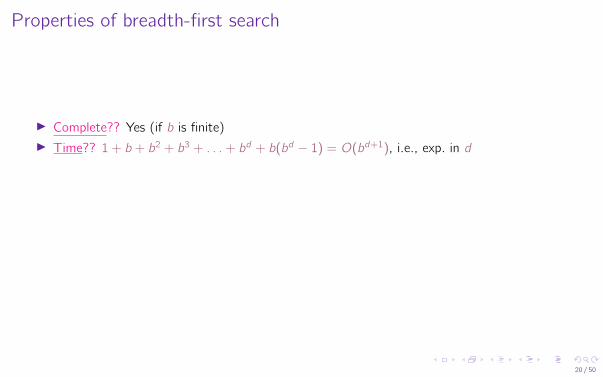
I Complete?? Yes (if b is finite)
I Time??I Space??I Optimal??
20 / 50

Properties of breadth-first search
I Complete?? Yes (if b is finite)I Time??
I Space??I Optimal??
20 / 50
Properties of breadth-first search
I Complete?? Yes (if b is finite)I Time?? 1+ b + b2 + b3 + . . .+ bd + b(bd − 1) = O(bd+1), i.e., exp. in d
I Space??I Optimal??
20 / 50

Properties of breadth-first search
I Complete?? Yes (if b is finite)I Time?? 1+ b + b2 + b3 + . . .+ bd + b(bd − 1) = O(bd+1), i.e., exp. in dI Space??
I Optimal??
20 / 50

Properties of breadth-first search
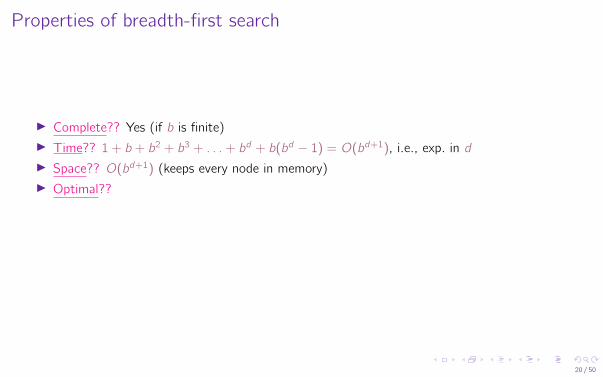
I Complete?? Yes (if b is finite)I Time?? 1+ b + b2 + b3 + . . .+ bd + b(bd − 1) = O(bd+1), i.e., exp. in dI Space?? O(bd+1) (keeps every node in memory)
I Optimal??
20 / 50
Properties of breadth-first search
I Complete?? Yes (if b is finite)I Time?? 1+ b + b2 + b3 + . . .+ bd + b(bd − 1) = O(bd+1), i.e., exp. in dI Space?? O(bd+1) (keeps every node in memory)I Optimal??
20 / 50

Properties of breadth-first search
I Complete?? Yes (if b is finite)I Time?? 1+ b + b2 + b3 + . . .+ bd + b(bd − 1) = O(bd+1), i.e., exp. in dI Space?? O(bd+1) (keeps every node in memory)I Optimal?? Yes (if cost = 1 per step); not optimal in general
Space is the big problem; can easily generate nodes at 100MB/secso 24hrs = 8640GB.
20 / 50
Uniform-cost search
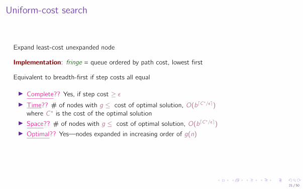
Expand least-cost unexpanded node
Implementation: fringe = queue ordered by path cost, lowest first
Equivalent to breadth-first if step costs all equal
I Complete?? Yes, if step cost ≥ εI Time?? # of nodes with g ≤ cost of optimal solution, O(bdC
∗/εe)where C ∗ is the cost of the optimal solution
I Space?? # of nodes with g ≤ cost of optimal solution, O(bdC∗/εe)
I Optimal?? Yes—nodes expanded in increasing order of g(n)
21 / 50

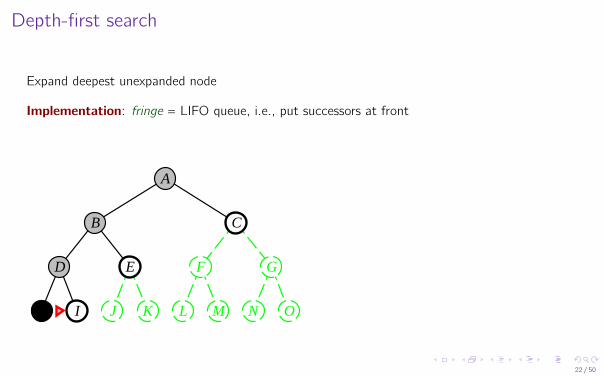
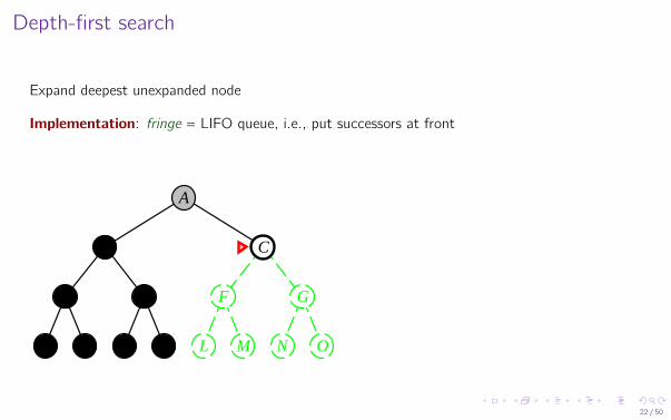
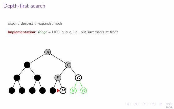
Depth-first search
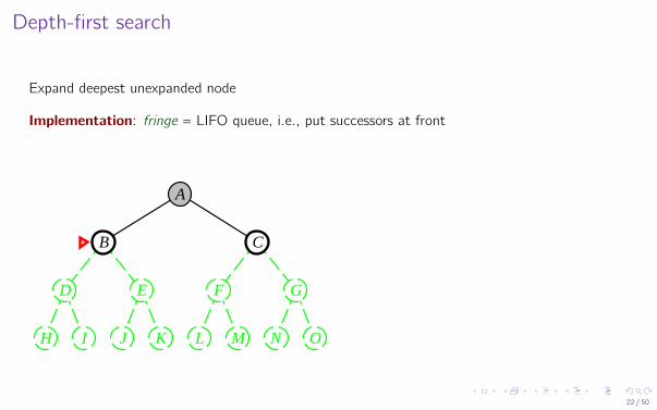
Expand deepest unexpanded node
Implementation: fringe = LIFO queue, i.e., put successors at front
A
B C
D E F G
H I J K L M N O
22 / 50
Depth-first search
Expand deepest unexpanded node
Implementation: fringe = LIFO queue, i.e., put successors at front
A
B C
D E F G
H I J K L M N O
22 / 50

Depth-first search
Expand deepest unexpanded node
Implementation: fringe = LIFO queue, i.e., put successors at front
A
B C
D E F G
H I J K L M N O
22 / 50

Depth-first search
Expand deepest unexpanded node
Implementation: fringe = LIFO queue, i.e., put successors at front
A
B C
D E F G
H I J K L M N O
22 / 50
Depth-first search
Expand deepest unexpanded node
Implementation: fringe = LIFO queue, i.e., put successors at front
A
B C
D E F G
H I J K L M N O
22 / 50

Depth-first search
Expand deepest unexpanded node
Implementation: fringe = LIFO queue, i.e., put successors at front
A
B C
D E F G
H I J K L M N O
22 / 50

Depth-first search
Expand deepest unexpanded node
Implementation: fringe = LIFO queue, i.e., put successors at front
A
B C
D E F G
H I J K L M N O
22 / 50

Depth-first search
Expand deepest unexpanded node
Implementation: fringe = LIFO queue, i.e., put successors at front
A
B C
D E F G
H I J K L M N O
22 / 50
Depth-first search
Expand deepest unexpanded node
Implementation: fringe = LIFO queue, i.e., put successors at front
A
B C
D E F G
H I J K L M N O
22 / 50

Depth-first search
Expand deepest unexpanded node
Implementation: fringe = LIFO queue, i.e., put successors at front
A
B C
D E F G
H I J K L M N O
22 / 50

Depth-first search
Expand deepest unexpanded node
Implementation: fringe = LIFO queue, i.e., put successors at front
A
B C
D E F G
H I J K L M N O
22 / 50
Depth-first search
Expand deepest unexpanded node
Implementation: fringe = LIFO queue, i.e., put successors at front
A
B C
D E F G
H I J K L M N O
22 / 50
Properties of depth-first search
I Complete??
I Time??I Space??I Optimal??
23 / 50
Properties of depth-first search
I Complete?? No: fails in infinite-depth spaces, spaces with loopsModify to avoid repeated states along path⇒ complete in finite spaces
I Time??I Space??I Optimal??
23 / 50
Properties of depth-first search
I Complete?? No: fails in infinite-depth spaces, spaces with loopsModify to avoid repeated states along path⇒ complete in finite spaces
I Time??
I Space??I Optimal??
23 / 50

Properties of depth-first search
I Complete?? No: fails in infinite-depth spaces, spaces with loopsModify to avoid repeated states along path⇒ complete in finite spaces
I Time?? O(bm): terrible if m is much larger than dbut if solutions are dense, may be much faster than breadth-first
I Space??I Optimal??
23 / 50
Properties of depth-first search
I Complete?? No: fails in infinite-depth spaces, spaces with loopsModify to avoid repeated states along path⇒ complete in finite spaces
I Time?? O(bm): terrible if m is much larger than dbut if solutions are dense, may be much faster than breadth-first
I Space??
I Optimal??
23 / 50

Properties of depth-first search
I Complete?? No: fails in infinite-depth spaces, spaces with loopsModify to avoid repeated states along path⇒ complete in finite spaces
I Time?? O(bm): terrible if m is much larger than dbut if solutions are dense, may be much faster than breadth-first
I Space?? O(bm), i.e., linear space!
I Optimal??
23 / 50

Properties of depth-first search
I Complete?? No: fails in infinite-depth spaces, spaces with loopsModify to avoid repeated states along path⇒ complete in finite spaces
I Time?? O(bm): terrible if m is much larger than dbut if solutions are dense, may be much faster than breadth-first
I Space?? O(bm), i.e., linear space!I Optimal??
23 / 50
Properties of depth-first search
I Complete?? No: fails in infinite-depth spaces, spaces with loopsModify to avoid repeated states along path⇒ complete in finite spaces
I Time?? O(bm): terrible if m is much larger than dbut if solutions are dense, may be much faster than breadth-first
I Space?? O(bm), i.e., linear space!I Optimal?? No
23 / 50
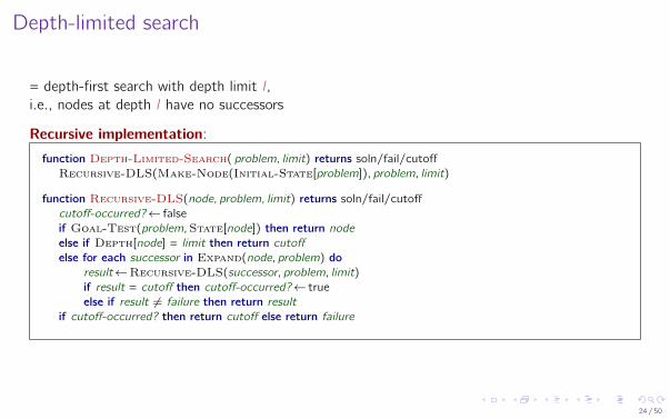
Depth-limited search
= depth-first search with depth limit l ,i.e., nodes at depth l have no successors
Recursive implementation:
function Depth-Limited-Search( problem, limit) returns soln/fail/cutoffRecursive-DLS(Make-Node(Initial-State[problem]), problem, limit)
function Recursive-DLS(node, problem, limit) returns soln/fail/cutoffcutoff-occurred?← falseif Goal-Test(problem,State[node]) then return nodeelse if Depth[node] = limit then return cutoffelse for each successor in Expand(node, problem) do
result←Recursive-DLS(successor, problem, limit)if result = cutoff then cutoff-occurred?← trueelse if result 6= failure then return result
if cutoff-occurred? then return cutoff else return failure
24 / 50
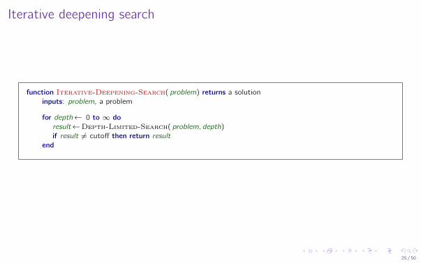
Iterative deepening search
function Iterative-Deepening-Search( problem) returns a solutioninputs: problem, a problem
for depth← 0 to ∞ doresult←Depth-Limited-Search( problem, depth)if result 6= cutoff then return result
end
25 / 50
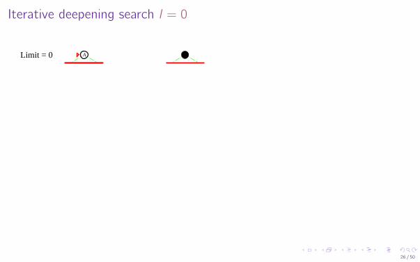
Iterative deepening search l = 0
Limit = 0 A A
26 / 50
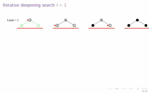
Iterative deepening search l = 1
Limit = 1 A
B C
A
B C
A
B C
A
B C
26 / 50

Iterative deepening search l = 2
Limit = 2 A
B C
D E F G
A
B C
D E F G
A
B C
D E F G
A
B C
D E F G
A
B C
D E F G
A
B C
D E F G
A
B C
D E F G
A
B C
D E F G
26 / 50

Iterative deepening search l = 3
Limit = 3
A
B C
D E F G
H I J K L M N O
A
B C
D E F G
H I J K L M N O
A
B C
D E F G
H I J K L M N O
A
B C
D E F G
H I J K L M N O
A
B C
D E F G
H I J K L M N O
A
B C
D E F G
H I J K L M N O
A
B C
D E F G
H I J K L M N O
A
B C
D E F G
H I J K L M N O
A
B C
D E F G
H I J K L M N O
A
B C
D E F G
H I J K L M N O
A
B C
D E F G
H J K L M N OI
A
B C
D E F G
H I J K L M N O
26 / 50

Properties of iterative deepening search
I Complete??
I Time??I Space??I Optimal??
27 / 50
Properties of iterative deepening search
I Complete?? Yes
I Time??I Space??I Optimal??
27 / 50

Properties of iterative deepening search
I Complete?? YesI Time??
I Space??I Optimal??
27 / 50
Properties of iterative deepening search
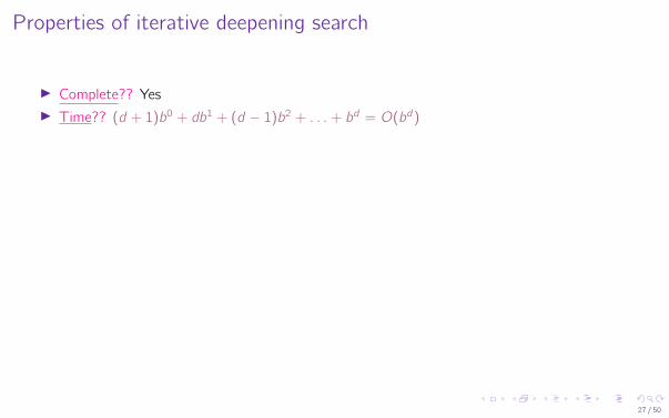
I Complete?? YesI Time?? (d + 1)b0 + db1 + (d − 1)b2 + . . .+ bd = O(bd)
I Space??I Optimal??
27 / 50

Properties of iterative deepening search
I Complete?? YesI Time?? (d + 1)b0 + db1 + (d − 1)b2 + . . .+ bd = O(bd)I Space??
I Optimal??
27 / 50

Properties of iterative deepening search
I Complete?? YesI Time?? (d + 1)b0 + db1 + (d − 1)b2 + . . .+ bd = O(bd)I Space?? O(bd)
I Optimal??
27 / 50

Properties of iterative deepening search
I Complete?? YesI Time?? (d + 1)b0 + db1 + (d − 1)b2 + . . .+ bd = O(bd)I Space?? O(bd)I Optimal??
27 / 50

Properties of iterative deepening search
I Complete?? YesI Time?? (d + 1)b0 + db1 + (d − 1)b2 + . . .+ bd = O(bd)I Space?? O(bd)I Optimal?? Yes, if step cost = 1
Can be modified to explore uniform-cost tree
Numerical comparison for b = 10 and d = 5, solution at far right leaf:
N(IDS) = 50+ 400+ 3, 000+ 20, 000+ 100, 000 = 123, 450
N(BFS) = 10+ 100+ 1, 000+ 10, 000+ 100, 000+ 999, 990 = 1, 111, 100
I IDS does better because other nodes at depth d are not expandedI BFS can be modified to apply goal test when a node is generated
27 / 50
Summary of algorithms
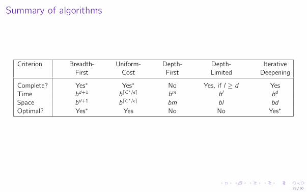
Criterion Breadth- Uniform- Depth- Depth- IterativeFirst Cost First Limited Deepening
Complete? Yes∗ Yes∗ No Yes, if l ≥ d YesTime bd+1 bdC
∗/εe bm bl bd
Space bd+1 bdC∗/εe bm bl bd
Optimal? Yes∗ Yes No No Yes∗
28 / 50
Repeated states
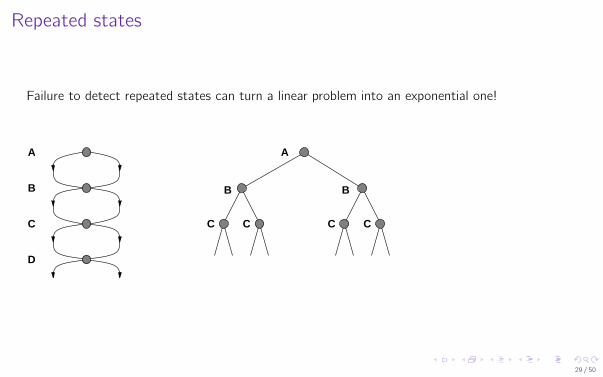
Failure to detect repeated states can turn a linear problem into an exponential one!
A
B
C
D
A
BB
CCCC
29 / 50

Graph search
function Graph-Search( problem, fringe) returns a solution, or failure
closed← an empty setfringe← Insert(Make-Node(Initial-State[problem]), fringe)loop do
if fringe is empty then return failurenode←Remove-Front(fringe)if Goal-Test(problem,State[node]) then return nodeif State[node] is not in closed then
add State[node] to closedfringe← InsertAll(Expand(node, problem), fringe)
end
30 / 50
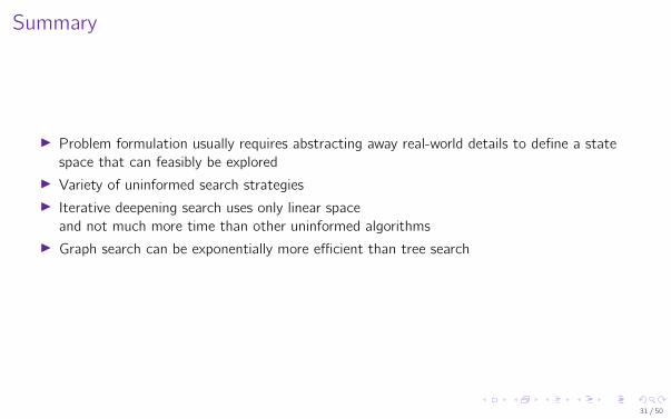
Summary
I Problem formulation usually requires abstracting away real-world details to define a statespace that can feasibly be explored
I Variety of uninformed search strategiesI Iterative deepening search uses only linear space
and not much more time than other uninformed algorithmsI Graph search can be exponentially more efficient than tree search
31 / 50
Informed Search Algorithms
I Best-first searchI A∗ searchI Heuristics
32 / 50

Review: Tree search
function Tree-Search( problem, fringe) returns a solution, or failurefringe← Insert(Make-Node(Initial-State[problem]), fringe)loop do
if fringe is empty then return failurenode←Remove-Front(fringe)if Goal-Test[problem] applied to State(node) succeeds return nodefringe← InsertAll(Expand(node, problem), fringe)
A strategy is defined by picking the order of node expansion
33 / 50

Best-first search
I Idea: use an evaluation function for each nodeI estimate of “desirability”⇒ Expand most desirable unexpanded node
I Implementation: fringe is a queue sorted in decreasing order of desirabilityI Special cases:
I greedy searchI A∗ search
34 / 50
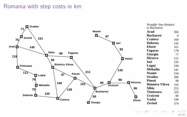
Romania with step costs in km
Bucharest
Giurgiu
Urziceni
Hirsova
Eforie
NeamtOradea
Zerind
Arad
Timisoara
LugojMehadia
DobretaCraiova
Sibiu
Fagaras
PitestiRimnicu Vilcea
Vaslui
Iasi
Straight−line distanceto Bucharest
0160242161
77151
241
366
193
178
25332980
199
244
380
226
234
374
98
Giurgiu
UrziceniHirsova
Eforie
Neamt
Oradea
Zerind
Arad
Timisoara
Lugoj
Mehadia
Dobreta
Craiova
Sibiu Fagaras
Pitesti
Vaslui
Iasi
Rimnicu Vilcea
Bucharest
71
75
118
111
70
75120
151
140
99
80
97
101
211
138
146 85
90
98
142
92
87
86
35 / 50

Greedy search
I Evaluation function h(n) (heuristic)= estimate of cost from n to the closest goalI E.g., hSLD(n) = straight-line distance from n to Bucharest
I Greedy search expands the node that appears to be closest to goal
36 / 50
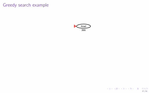
Greedy search example
Arad
366
37 / 50

Greedy search example
Zerind
Arad
Sibiu Timisoara
253 329 374
37 / 50

Greedy search example
Rimnicu Vilcea
Zerind
Arad
Sibiu
Arad Fagaras Oradea
Timisoara
329 374
366 176 380 193
37 / 50
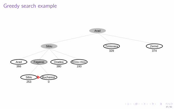
Greedy search example
Rimnicu Vilcea
Zerind
Arad
Sibiu
Arad Fagaras Oradea
Timisoara
Sibiu Bucharest
329 374
366 380 193
253 0
37 / 50

Properties of greedy search
I Complete??
I Time??I Space??I Optimal??
38 / 50
Properties of greedy search
I Complete?? No–can get stuck in loops, e.g.,Iasi → Neamt → Iasi → Neamt →Complete in finite space with repeated-state checking
I Time??I Space??I Optimal??
38 / 50

Properties of greedy search
I Complete?? No–can get stuck in loops, e.g.,Iasi → Neamt → Iasi → Neamt →Complete in finite space with repeated-state checking
I Time??
I Space??I Optimal??
38 / 50

Properties of greedy search
I Complete?? No–can get stuck in loops, e.g.,Iasi → Neamt → Iasi → Neamt →Complete in finite space with repeated-state checking
I Time?? O(bm), but a good heuristic can give dramatic improvement
I Space??I Optimal??
38 / 50

Properties of greedy search
I Complete?? No–can get stuck in loops, e.g.,Iasi → Neamt → Iasi → Neamt →Complete in finite space with repeated-state checking
I Time?? O(bm), but a good heuristic can give dramatic improvementI Space??
I Optimal??
38 / 50

Properties of greedy search
I Complete?? No–can get stuck in loops, e.g.,Iasi → Neamt → Iasi → Neamt →Complete in finite space with repeated-state checking
I Time?? O(bm), but a good heuristic can give dramatic improvementI Space?? O(bm)—keeps all nodes in memory
I Optimal??
38 / 50

Properties of greedy search
I Complete?? No–can get stuck in loops, e.g.,Iasi → Neamt → Iasi → Neamt →Complete in finite space with repeated-state checking
I Time?? O(bm), but a good heuristic can give dramatic improvementI Space?? O(bm)—keeps all nodes in memoryI Optimal??
38 / 50
Properties of greedy search
I Complete?? No–can get stuck in loops, e.g.,Iasi → Neamt → Iasi → Neamt →Complete in finite space with repeated-state checking
I Time?? O(bm), but a good heuristic can give dramatic improvementI Space?? O(bm)—keeps all nodes in memoryI Optimal?? No
38 / 50

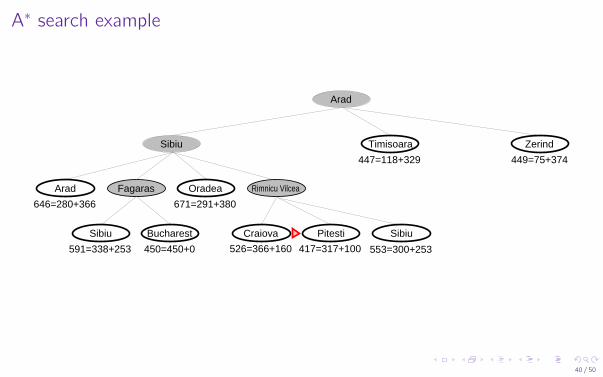
A∗ search
I Idea: avoid expanding paths that are already expensiveI Evaluation function f (n) = g(n) + h(n)
I g(n) = cost so far to reach nh(n) = estimated cost to goal from nf (n) = estimated total cost of path through n to goal
I A∗ search uses an admissible heuristici.e., h(n) ≤ h∗(n) where h∗(n) is the true cost from n.(Also require h(n) ≥ 0, so h(G ) = 0 for any goal G .)I E.g., hSLD(n) never overestimates the actual road distance
I Theorem: A∗ search is optimal
39 / 50

A∗ search example
Arad
366=0+366
40 / 50

A∗ search example
Zerind
Arad
Sibiu Timisoara
447=118+329 449=75+374393=140+253
40 / 50

A∗ search example
Zerind
Arad
Sibiu
Arad
Timisoara
Rimnicu VilceaFagaras Oradea
447=118+329 449=75+374
646=280+366 413=220+193415=239+176 671=291+380
40 / 50

A∗ search example
Zerind
Arad
Sibiu
Arad
Timisoara
Fagaras Oradea
447=118+329 449=75+374
646=280+366 415=239+176
Rimnicu Vilcea
Craiova Pitesti Sibiu
526=366+160 553=300+253417=317+100
671=291+380
40 / 50
A∗ search example
Zerind
Arad
Sibiu
Arad
Timisoara
Sibiu Bucharest
Rimnicu VilceaFagaras Oradea
Craiova Pitesti Sibiu
447=118+329 449=75+374
646=280+366
591=338+253 450=450+0 526=366+160 553=300+253417=317+100
671=291+380
40 / 50

A∗ search example
Zerind
Arad
Sibiu
Arad
Timisoara
Sibiu Bucharest
Rimnicu VilceaFagaras Oradea
Craiova Pitesti Sibiu
Bucharest Craiova Rimnicu Vilcea
418=418+0
447=118+329 449=75+374
646=280+366
591=338+253 450=450+0 526=366+160 553=300+253
615=455+160 607=414+193
671=291+380
40 / 50

Optimality of A∗ (standard proof)Suppose some suboptimal goal G2 has been generated and is in the queue. Let n be anunexpanded node on a shortest path to an optimal goal G1.
G
n
G2
Start
f (G2) = g(G2) since h(G2) = 0
> g(G1) since G2 is suboptimal≥ f (n) since h is admissible
Since f (G2) > f (n), A∗ will never select G2 for expansion41 / 50
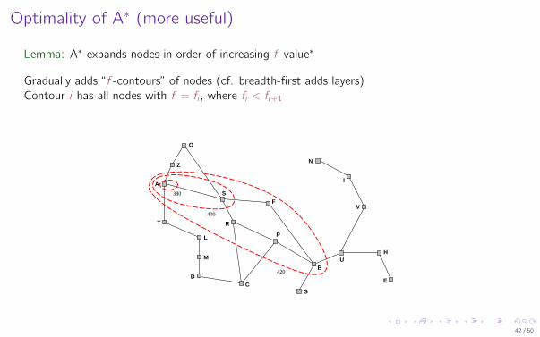
Optimality of A∗ (more useful)
Lemma: A∗ expands nodes in order of increasing f value∗
Gradually adds “f -contours” of nodes (cf. breadth-first adds layers)Contour i has all nodes with f = fi , where fi < fi+1
O
Z
A
T
L
M
DC
R
F
P
G
BU
H
E
V
I
N
380
400
420
S
42 / 50

Properties of A∗
I Complete??I Time??I Space??I Optimal??
43 / 50
Properties of A∗
I Complete?? Yes, unless there are infinitely many nodes with f ≤ f (G )
I Time??I Space??I Optimal??
43 / 50

Properties of A∗
I Complete?? Yes, unless there are infinitely many nodes with f ≤ f (G )
I Time?? Exponential in [relative error in h × length of soln.]I Space??I Optimal??
43 / 50

Properties of A∗
I Complete?? Yes, unless there are infinitely many nodes with f ≤ f (G )
I Time?? Exponential in [relative error in h × length of soln.]I Space?? Keeps all nodes in memoryI Optimal??
43 / 50

Properties of A∗
I Complete?? Yes, unless there are infinitely many nodes with f ≤ f (G )
I Time?? Exponential in [relative error in h × length of soln.]I Space?? Keeps all nodes in memoryI Optimal?? Yes—cannot expand fi+1 until fi is finished
43 / 50

Properties of A∗
I Complete?? Yes, unless there are infinitely many nodes with f ≤ f (G )
I Time?? Exponential in [relative error in h × length of soln.]I Space?? Keeps all nodes in memoryI Optimal?? Yes—cannot expand fi+1 until fi is finished
A∗ expands all nodes with f (n) < C ∗
A∗ expands some nodes with f (n) = C ∗
A∗ expands no nodes with f (n) > C ∗
43 / 50

Proof of lemma: Consistency
A heuristic is consistent if
h(n) ≤ c(n, a, n′) + h(n′)
If h is consistent, we have
f (n′) = g(n′) + h(n′)
= g(n) + c(n, a, n′) + h(n′)
≥ g(n) + h(n)
= f (n)
I.e., f (n) is nondecreasing along any path.
44 / 50

Admissible heuristics
E.g., for the 8-puzzle:
h1(n) = number of misplaced tilesh2(n) = total Manhattan distance(i.e., no. of squares from desired location of each tile)
2
Start State Goal State
51 3
4 6
7 8
5
1
2
3
4
6
7
8
5
h1(S) =??h2(S) =??
45 / 50

Admissible heuristics
E.g., for the 8-puzzle:
h1(n) = number of misplaced tilesh2(n) = total Manhattan distance(i.e., no. of squares from desired location of each tile)
2
Start State Goal State
51 3
4 6
7 8
5
1
2
3
4
6
7
8
5
h1(S) =?? 6h2(S) =?? 4+0+3+3+1+0+2+1 = 14
46 / 50
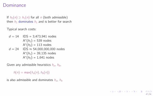
Dominance
If h2(n) ≥ h1(n) for all n (both admissible)then h2 dominates h1 and is better for search
Typical search costs:
d = 14 IDS = 3,473,941 nodesA∗(h1) = 539 nodesA∗(h2) = 113 nodes
d = 24 IDS ≈ 54,000,000,000 nodesA∗(h1) = 39,135 nodesA∗(h2) = 1,641 nodes
Given any admissible heuristics ha, hb,
h(n) = max(ha(n), hb(n))
is also admissible and dominates ha, hb
47 / 50

Relaxed problems
I Admissible heuristics can be derived from the exactsolution cost of a relaxed version of the problem
I If the rules of the 8-puzzle are relaxed so that a tile can move anywhere, then h1(n) givesthe shortest solution
I If the rules are relaxed so that a tile can move to any adjacent square, then h2(n) gives theshortest solution
I Key point: the optimal solution cost of a relaxed problemis no greater than the optimal solution cost of the real problem
48 / 50
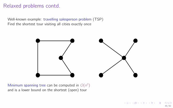
Relaxed problems contd.
Well-known example: travelling salesperson problem (TSP)Find the shortest tour visiting all cities exactly once
Minimum spanning tree can be computed in O(n2)and is a lower bound on the shortest (open) tour
49 / 50

Summary
I Heuristic functions estimate costs of shortest pathsI Good heuristics can dramatically reduce search costI Greedy best-first search expands lowest h
I incomplete and not always optimalI A∗ search expands lowest g + h
I complete and optimalI also optimally efficient (up to tie-breaks, for forward search)
I Admissible heuristics can be derived from exact solution of relaxed problems
50 / 50