An analytic function whose only singularities in the finite plane are poles is called a meromorphic function.Examples are rational functions with nonconstant denominator, , and

In this section we used Laurent series for investigating singularities. In the next sectionwe shall use these series for an elegant integration method.

�csc z.tan z, cot z, sec z

SEC. 16.3 Residue Integration Method 719

1–10 ZEROSDetermine the location and order of the zeros.

1. 2.

3. 4.

5. 6.

7.

8.

9.

10.

11. Zeros. If is analytic and has a zero of order n atshow that has a zero of order 2n at

12. TEAM PROJECT. Zeros. (a) Derivative. Show thatif has a zero of order at then has a zero of order at

(b) Poles and zeros. Prove Theorem 4.

(c) Isolated k-points. Show that the points at whicha nonconstant analytic function has a given valuek are isolated.

(d) Identical functions. If and are analyticin a domain D and equal at a sequence of points inD that converges in D, show that in D.f1(z) � f2(z)

zn

f2(z)f1(z)

f (z)

z0.n � 1f r(z)z � z0,n 1f (z)

z0.f 2(z)z � z0,f (z)

(z2 � 8)3(exp (z2) � 1)

sin 2z cos 2z

(sin z � 1)3

z4 � (1 � 8i) z2 � 8i

cosh4 zz�2 sin2 pz

tan2 2z(z � 81i)4

(z4 � 81)3sin4 12 z

13–22 SINGULARITIES

Determine the location of the singularities, including thoseat infinity. For poles also state the order. Give reasons.

13.

14.

15. 16.

17. 18.

19. 20.

21. 22.

23. Essential singularity. Discuss in a similar way asis discussed in Example 3 of the text.

24. Poles. Verify Theorem 1 for ProveTheorem 1.

25. Riemann sphere. Assuming that we let the image ofthe x-axis be the meridians and describe andsketch (or graph) the images of the following regionson the Riemann sphere: (a) (b) the lowerhalf-plane, (c) 1

2 ƒ z ƒ 2.ƒ z ƒ 100,

180°,0°

f (z) � z�3 � z�1.

e1>ze1>z2

(z � p)�1 sin ze1>(z�1)>(ez � 1)

1>(cos z � sin z)1>(ez � e2z)

z3 exp a 1z � 1

bcot4 z

tan pzz exp (1>(z � 1 � i)2)

ez�i �2

z � i�

8(z � i)3

1

(z � 2i)2 �z

z � i�

z � 1

(z � i)2

P R O B L E M S E T 1 6 . 2

16.3 Residue Integration MethodWe now cover a second method of evaluating complex integrals. Recall that we solvedcomplex integrals directly by Cauchy’s integral formula in Sec. 14.3. In Chapter 15 welearned about power series and especially Taylor series. We generalized Taylor series toLaurent series (Sec. 16.1) and investigated singularities and zeroes of various functions(Sec. 16.2). Our hard work has paid off and we see how much of the theoretical groundworkcomes together in evaluating complex integrals by the residue method.

The purpose of Cauchy’s residue integration method is the evaluation of integrals

taken around a simple closed path C. The idea is as follows.If is analytic everywhere on C and inside C, such an integral is zero by Cauchy’s

integral theorem (Sec. 14.2), and we are done.f (z)

�C

f (z) dz

c16.qxd 11/1/10 6:57 PM Page 719

720 CHAP. 16 Laurent Series. Residue Integration

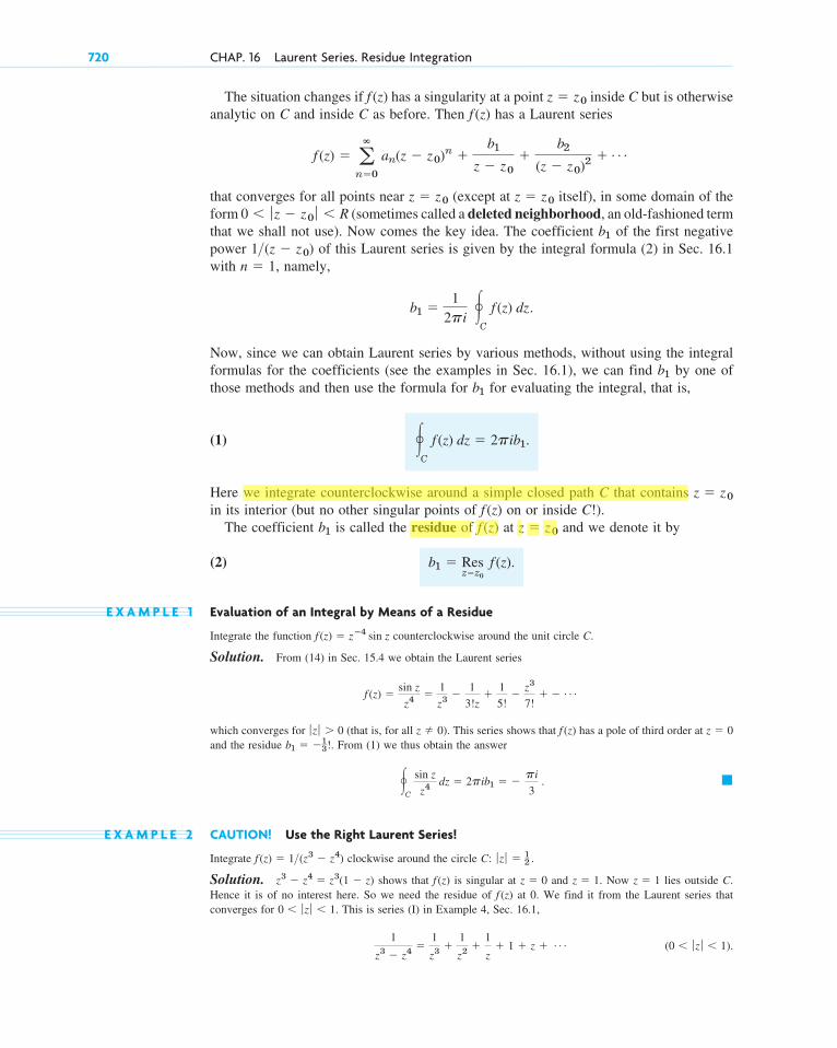
The situation changes if has a singularity at a point inside C but is otherwiseanalytic on C and inside C as before. Then has a Laurent series

that converges for all points near (except at itself), in some domain of theform (sometimes called a deleted neighborhood, an old-fashioned termthat we shall not use). Now comes the key idea. The coefficient of the first negativepower of this Laurent series is given by the integral formula (2) in Sec. 16.1with namely,

Now, since we can obtain Laurent series by various methods, without using the integralformulas for the coefficients (see the examples in Sec. 16.1), we can find by one ofthose methods and then use the formula for for evaluating the integral, that is,

(1)

Here we integrate counterclockwise around a simple closed path C that contains in its interior (but no other singular points of on or inside C!).

The coefficient is called the residue of at and we denote it by

(2)

E X A M P L E 1 Evaluation of an Integral by Means of a Residue

Integrate the function counterclockwise around the unit circle C.

Solution. From (14) in Sec. 15.4 we obtain the Laurent series

which converges for (that is, for all This series shows that has a pole of third order at and the residue . From (1) we thus obtain the answer

E X A M P L E 2 CAUTION! Use the Right Laurent Series!

Integrate clockwise around the circle C: .

Solution. shows that is singular at and Now lies outside C.Hence it is of no interest here. So we need the residue of at 0. We find it from the Laurent series thatconverges for This is series (I) in Example 4, Sec. 16.1,

(0 � ƒ z ƒ � 1).1

z3 � z4 �1

z3 �1

z2 �1

z� 1 � z � Á

0 � ƒ z ƒ � 1.f (z)

z � 1z � 1.z � 0f (z)z3 � z4 � z3(1 � z)

ƒ z ƒ � 12 f (z) � 1>(z3 � z4)

��C

sin z

z4 dz � 2pib1 � � pi

3 .

b1 � �13 !

z � 0f (z)z � 0).ƒ z ƒ 0

f (z) �sin z

z4 �1

z3 �1

3!z�

1

5!�

z3

7!� � Á

f (z) � z�4 sin z

b1 � Resz�z0

f (z).

z � z0f (z)b1

f (z)z � z0

�C

f (z) dz � 2pib1.

b1

b1

b1 �1

2pi �

C

f (z) dz.

n � 1,1>(z � z0)

b1

0 � ƒ z � z0 ƒ � Rz � z0z � z0

f (z) � a�

n�0

an(z � z0)n �b1

z � z0�

b2

(z � z0)2 � Á

f (z)z � z0f (z)

c16.qxd 11/1/10 6:57 PM Page 720

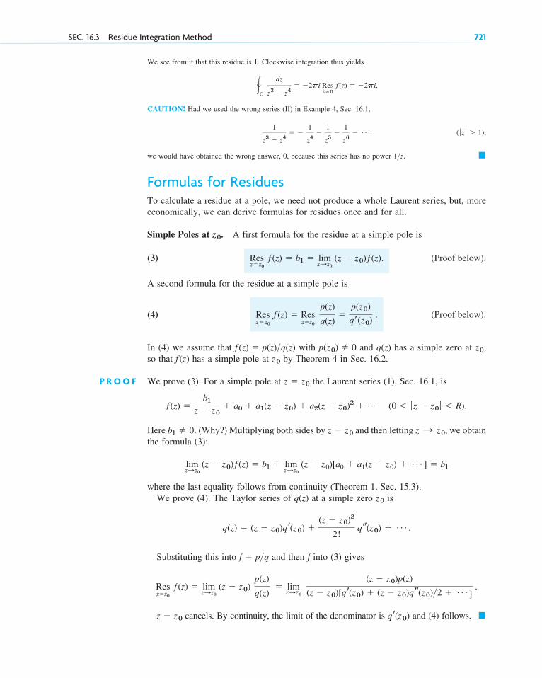
We see from it that this residue is 1. Clockwise integration thus yields

CAUTION! Had we used the wrong series (II) in Example 4, Sec. 16.1,

we would have obtained the wrong answer, 0, because this series has no power

Formulas for ResiduesTo calculate a residue at a pole, we need not produce a whole Laurent series, but, moreeconomically, we can derive formulas for residues once and for all.

Simple Poles at . A first formula for the residue at a simple pole is

(3)

A second formula for the residue at a simple pole is

(4)

In (4) we assume that with and has a simple zero at so that has a simple pole at by Theorem 4 in Sec. 16.2.

P R O O F We prove (3). For a simple pole at the Laurent series (1), Sec. 16.1, is

Here (Why?) Multiplying both sides by and then letting we obtainthe formula (3):

where the last equality follows from continuity (Theorem 1, Sec. 15.3).We prove (4). The Taylor series of at a simple zero is

Substituting this into and then f into (3) gives

cancels. By continuity, the limit of the denominator is and (4) follows. �qr(z0)z � z0

Resz�z0

f (z) � limz:z0

(z � z0)

p(z)

q(z) � lim

z:z0

(z � z0)p(z)

(z � z0)[qr(z0) � (z � z0)qs(z0)>2 � Á ] .

f � p>q

q(z) � (z � z0)qr(z0) �(z � z0)2

2! qs(z0) � Á .

z0q(z)

limz:z0

(z � z0) f (z) � b1 � limz:z0

(z � z0)[a0 � a1(z � z0) � Á ] � b1

z : z0,z � z0b1 � 0.

f (z) �b1

z � z0� a0 � a1(z � z0) � a2(z � z0)2 � Á (0 � ƒ z � z0 ƒ � R).

z � z0

z0f (z)z0,q(z)p(z0) � 0f (z) � p(z)>q(z)

(Proof below).Resz�z0

f (z) � Resz�z0

p(z)

q(z)�

p(z0)

qr(z0) .

(Proof below).Resz�z0

f (z) � b1 � limz:z0

(z � z0) f (z).

z0

�1>z.

( ƒ z ƒ 1),1

z3 � z4� �

1

z4�

1

z5�

1

z6� Á

�C

dz

z3 � z4� �2pi Res

z�0 f (z) � �2pi.

SEC. 16.3 Residue Integration Method 721

c16.qxd 11/1/10 6:57 PM Page 721

E X A M P L E 3 Residue at a Simple Pole

has a simple pole at i because , and (3) gives the residue

By (4) with and we confirm the result,

Poles of Any Order at . The residue of at an mth-order pole at is

(5)

In particular, for a second-order pole

P R O O F We prove (5). The Laurent series of converging near (except at itself) is (Sec. 16.2)

where The residue wanted is Multiplying both sides by gives

We see that is now the coefficient of the power of the power series ofHence Taylor’s theorem (Sec. 15.4) gives (5):

E X A M P L E 4 Residue at a Pole of Higher Order

has a pole of second order at because the denominator equals(verify!). From we obtain the residue

�Resz�1

f (z) � limz:1

d

dz [(z � 1)2 f (z)] � lim

z:1

d

dz a 50z

z � 4 b �

200

52 � 8.

(5*)(z � 4)(z � 1)2z � 1f (z) � 50z>(z3 � 2z2 � 7z � 4)

� �1

(m � 1)!

dm�1

dzm�1 [(z � z0)mf (z)].

b1 �1

(m � 1)! g(m�1)(z0)

g(z) � (z � z0)mf (z).(z � z0)m�1b1

(z � z0)mf (z) � bm � bm�1(z � z0) � Á � b1(z � z0)m�1 � a0(z � z0)m � Á .

(z � z0)mb1.bm � 0.

f (z) �bm

(z � z0)m �bm�1

(z � z0)m�1 � Á �b1

z � z0� a0 � a1(z � z0) � Á

z0z0f (z)

Resz�z0

f (z) � limz:z0

{[(z � z0)2f (z)]r}.(5*)

(m � 2),

Resz�z0

f (z) �

1(m � 1)!

limz:z

0

e dm�1

dzm�1 c (z � z0)mf (z) d f .

z0f (z)z0

�Resz�i

9z � i

z(z2 � 1)� c 9z � i

3z2 � 1 d

z�i

�10i

�2� �5i.

qr(z) � 3z2 � 1p(i) � 9i � i

Resz�i

9z � i

z(z2 � 1)� lim

z:i (z � i)

9z � i

z(z � i)(z � i)� c 9z � i

z(z � i) d

z�i

�10i

�2� �5i.

z2 � 1 � (z � i)(z � i)f (z) � (9z � i)>(z3 � z)

722 CHAP. 16 Laurent Series. Residue Integration

c16.qxd 11/1/10 6:57 PM Page 722

z1

z2

z3

C

Fig. 373. Residue theorem

Several Singularities Inside the Contour. Residue TheoremResidue integration can be extended from the case of a single singularity to the case ofseveral singularities within the contour C. This is the purpose of the residue theorem. Theextension is surprisingly simple.

T H E O R E M 1 Residue Theorem

Let be analytic inside a simple closed path C and on C, except for finitely manysingular points inside C. Then the integral of taken counterclockwisearound C equals times the sum of the residues of at

(6) �C

f (z) dz � 2piak

j�1

Resz�zj

f (z).

z1, Á , zk :f (z)2pif (z)z1, z2, Á , zk

f (z)

SEC. 16.3 Residue Integration Method 723

P R O O F We enclose each of the singular points in a circle with radius small enough thatthose k circles and C are all separated (Fig. 373 where Then is analytic in themultiply connected domain D bounded by C and and on the entire boundaryof D. From Cauchy’s integral theorem we thus have

(7)

the integral along C being taken counterclockwise and the other integrals clockwise (as inFigs. 354 and 355, Sec. 14.2). We take the integrals over to the right andcompensate the resulting minus sign by reversing the sense of integration. Thus,

(8)

where all the integrals are now taken counterclockwise. By (1) and (2),

so that (8) gives (6) and the residue theorem is proved. �

j � 1, Á , k,�Cj

f (z) dz � 2pi Res

z�zj

f (z),

�C

f (z) dz � �C1

f (z) dz � �C2

f (z) dz � Á � �Ck

f (z) dz

C1, Á , Ck

�C

f (z) dz � �C1

f (z) dz � �C2

f (z) dz � Á � �Ck

f (z) dz � 0,

C1, Á , Ck

f (z)k � 3).Cjz j

c16.qxd 11/1/10 6:57 PM Page 723

This important theorem has various applications in connection with complex and real integrals.Let us first consider some complex integrals. (Real integrals follow in the next section.)

E X A M P L E 5 Integration by the Residue Theorem. Several Contours

Evaluate the following integral counterclockwise around any simple closed path such that (a) 0 and 1 are insideC, (b) 0 is inside, 1 outside, (c) 1 is inside, 0 outside, (d) 0 and 1 are outside.

Solution. The integrand has simple poles at 0 and 1, with residues [by (3)]

[Confirm this by (4).] Answer: (a) (b) (c) (d) 0.

E X A M P L E 6 Another Application of the Residue Theorem

Integrate counterclockwise around the circle C: .

Solution. is not analytic at but all these points lie outside the contour C. Becauseof the denominator the given function has simple poles at We thus obtain from(4) and the residue theorem

E X A M P L E 7 Poles and Essential Singularities

Evaluate the following integral, where C is the ellipse (counterclockwise, sketch it).

Solution. Since at and the first term of the integrand has simple poles at insideC, with residues [by (4); note that

and simple poles at which lie outside C, so that they are of no interest here. The second term of the integrandhas an essential singularity at 0, with residue as obtained from

Answer: by the residue theorem. �2pi(� 116 � 1

16 � 12 p2) � p(p2 � 1

4 )i � 30.221i

( ƒ z ƒ 0).zep>z � z a1 �p

z�p2

2!z2 �p3

3!z3 � Á b � z � p �p2

2 #

1

z� Á

p2>2�2,

Resz��2i

zepz

z4 � 16� c zepz

4z3 dz��2i

�� 1

16

Resz�2i

zepz

z4 � 16� c zepz

4z3 dz�2i

� � 1

16 ,

e2pi � 1]�2i�2,�2iz4 � 16 � 0

�C

a zepz

z4 � 16� zep>zb dz.

9x2 � y2 � 9

� � 2pi tan 1 � 9.7855i.

� 2pi a tan z

2z `

z�1�

tan z

2z`z��1

b

�C

tan z

z2 � 1 dz � 2pi aRes

z�1

tan z

z2 � 1 � Res

z��1

tan z

z2 � 1 b

�1.z2 � 1 � (z � 1)(z � 1)�p>2, �3p>2, Á ,tan z

ƒ z ƒ � 32 (tan z)>(z2 � 1)

�2pi,�8pi,2pi(�4 � 1) � �6pi,

Resz�0

4 � 3z

z(z � 1)� c 4 � 3z

z � 1 d

z�0

� �4, Resz�1

4 � 3z

z(z � 1)� c 4 � 3z

z d

z�1

� 1.

�C

4 � 3z

z2 � z dz

724 CHAP. 16 Laurent Series. Residue Integration

c16.qxd 11/1/10 6:57 PM Page 724

16.4 Residue Integration of Real IntegralsSurprisingly, residue integration can also be used to evaluate certain classes of complicatedreal integrals. This shows an advantage of complex analysis over real analysis or calculus.

Integrals of Rational Functions of cos � and sin �We first consider integrals of the type

(1) J � �2p

0

F(cos u, sin u) du

SEC. 16.4 Residue Integration of Real Integrals 725

1. Verify the calculations in Example 3 and find the otherresidues.

2. Verify the calculations in Example 4 and find the otherresidue.

3–12 RESIDUESFind all the singularities in the finite plane and thecorresponding residues. Show the details.

3. 4.

5. 6.

7. 8.

9. 10.

11. 12.

13. CAS PROJECT. Residue at a Pole. Write a programfor calculating the residue at a pole of any order in thefinite plane. Use it for solving Probs. 5–10.

14–25 RESIDUE INTEGRATIONEvaluate (counterclockwise). Show the details.

14.

15. �C

tan 2pz dz, C: ƒ z � 0.2 ƒ � 0.2

�C

z � 23

z2 � 4z � 5 dz, C: ƒ z � 2 � i ƒ � 3.2

e1>(1�z)ez

(z � pi)3

z4

z2 � iz � 2

1

1 � ez

p

(z2 � 1)2cot pz

tan z8

1 � z2

cos z

z4

sin 2z

z6

16. the unit circle

17.

18.

19.

20.

21.

22. the unit circle

23. the unit circle

24.

25. �C

z cosh pz

z4 � 13z2 � 36 dz, ƒ z ƒ � p

�C

exp (�z2)

sin 4z dz, C: ƒ z ƒ � 1.5

�C

30z2 � 23z � 5

(2z � 1)2(3z � 1) dz, C

�C

z2 sin z

4z2 � 1 dz, C

�C

cos pz

z5 dz, C: ƒ z ƒ � 1

2

�C

dz

(z2 � 1)3 , C: ƒ z � i ƒ � 3

�C

sinh z

2z � i dz, C: ƒ z � 2i ƒ � 2

�C

z � 1

z4 � 2z3 dz, C: ƒ z � 1 ƒ � 2

�C

ez

cos z dz, C: ƒ z � pi>2 ƒ � 4.5

�C

e1>z dz, C:

P R O B L E M S E T 1 6 . 3

c16.qxd 11/1/10 6:57 PM Page 725

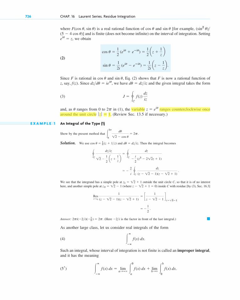
where is a real rational function of and [for example, and is finite (does not become infinite) on the interval of integration. Setting

we obtain

(2)

Since F is rational in and Eq. (2) shows that F is now a rational function ofz, say, Since we have and the given integral takes the form

(3)

and, as ranges from 0 to in (1), the variable ranges counterclockwise oncearound the unit circle (Review Sec. 13.5 if necessary.)

E X A M P L E 1 An Integral of the Type (1)

Show by the present method that

Solution. We use and Then the integral becomes

We see that the integrand has a simple pole at outside the unit circle C, so that it is of no interesthere, and another simple pole at (where inside C with residue [by (3), Sec. 16.3]

Answer: (Here is the factor in front of the last integral.)

As another large class, let us consider real integrals of the form

(4)

Such an integral, whose interval of integration is not finite is called an improper integral,and it has the meaning

��

��

f (x) dx � lima:��

�0

a f (x) dx � lim

b:� �

b

0 f (x) dx.(5r)

��

��

f (x) dx.

��2>i2pi(�2>i)(�12 ) � 2p.

� �

1

2 .

Resz�z2

1

(z � 12 � 1)(z � 12 � 1) � c 1

z � 12 � 1 d

z�12�1

z � 12 � 1 � 0)z2 � 12 � 1z1 � 12 � 1

� � 2

i �

C

dz

(z � 12 � 1)(z � 12 � 1) .

�C

dz>iz

12 �1

2 az �

1z

b� �

C

dz

�

i

2 (z2 � 212z � 1)

du � dz>iz.cos u � 12 (z � 1>z)

�2p

0

du

12 � cos u� 2p.

ƒ z ƒ � 1.z � eiu2pu

J � �C

f (z) dz

iz

du � dz>izdz>du � ieiu,f (z).sin u,cos u

sin u �12i

(eiu � e�iu) �12i

az �1zb .

cos u �12

(eiu � e�iu) �12

az �1z

b

eiu � z,(5 � 4 cos u)]

(sin2 u)>sin ucos uF(cos u, sin u)

726 CHAP. 16 Laurent Series. Residue Integration

c16.qxd 11/1/10 6:57 PM Page 726

If both limits exist, we may couple the two independent passages to and , and write

(5)

The limit in (5) is called the Cauchy principal value of the integral. It is written

pr. v.

It may exist even if the limits in do not. Example:

We assume that the function in (4) is a real rational function whose denominatoris different from zero for all real x and is of degree at least two units higher than thedegree of the numerator. Then the limits in exist, and we may start from (5). Weconsider the corresponding contour integral

around a path C in Fig. 374. Since is rational, has finitely many poles in theupper half-plane, and if we choose R large enough, then C encloses all these poles. Bythe residue theorem we then obtain

where the sum consists of all the residues of at the points in the upper half-plane atwhich has a pole. From this we have

(6)

We prove that, if the value of the integral over the semicircle S approacheszero. If we set then S is represented by and as z ranges along S, thevariable ranges from 0 to Since, by assumption, the degree of the denominator of

is at least two units higher than the degree of the numerator, we have

( ƒ z ƒ � R R0)ƒ f (z) ƒ �k

ƒ z ƒ2

f (z)p.u

R � const,z � Reiu,R : �,

�R

�R

f (x) dx � 2pia Res f (z) � �S

f (z) dz.

f (z)f (z)

�C

f (z) dz � �

S f (z) dz � �

R

�R f (x) dx � 2pi a Res f (z)

f (z)f (x)

�C

f (z) dz(5*)

(5r)

f (x)

limR:� �

R

�R

x dx � limR:�

aR2

2�

R2

2 b � 0, but lim

b:��b

0

x dx � �.

(5r)

��

��

f (x) dx.

��

��

f (x) dx � limR:��

R

�R f (x) dx.

���

SEC. 16.4 Residue Integration of Real Integrals 727

Fig. 374. Path C of the contour integral in (5*)

y

x–R R

S

c16.qxd 11/1/10 6:57 PM Page 727

for sufficiently large constants k and By the ML-inequality in Sec. 14.1,

Hence, as R approaches infinity, the value of the integral over S approaches zero, and (5)and (6) yield the result

(7)

where we sum over all the residues of at the poles of in the upper half-plane.

E X A M P L E 2 An Improper Integral from 0 to

Using (7), show that

��

0

dx

1 � x4�p

212 .

�

f (z)f (z)

��

��

f (x) dx � 2piaRes f (z)

(R R0).` �S

f (z) dz ` �

k

R2 pR �

kp

R

R0.

728 CHAP. 16 Laurent Series. Residue Integration

z1

z4

z2

z3

y

x

Fig. 375. Example 2

Solution. Indeed, has four simple poles at the points (make a sketch)

The first two of these poles lie in the upper half-plane (Fig. 375). From (4) in the last section we find the residues

(Here we used and By (1) in Sec. 13.6 and (7) in this section,

��

��

dx

1 � x4 � � 2pi

4 (epi>4 � e�pi>4) � �

2pi

4 # 2i sin

p

4� p sin

p

4�p

12 .

e�2pi � 1.)epi � �1

Resz�z2

f (z) � c 1

(1 � z4)r d

z�z2

� c 1

4z3 dz�z2

�1

4 e�9pi>4 �

1

4 e�pi>4.

Resz�z1

f (z) � c 1

(1 � z4)r d

z�z1

� c 1

4z3 dz�z1

�1

4 e�3pi>4 � �

1

4 epi>4.

z1 � epi>4, z2 � e3pi>4, z3 � e�3pi>4, z4 � e�pi>4.

f (z) � 1>(1 � z4)

c16.qxd 11/1/10 6:57 PM Page 728

Since is an even function, we thus obtain, as asserted,

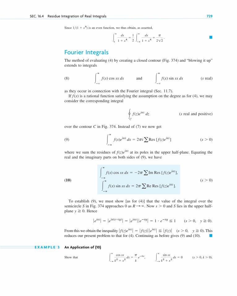
Fourier IntegralsThe method of evaluating (4) by creating a closed contour (Fig. 374) and “blowing it up”extends to integrals

(8) and (s real)

as they occur in connection with the Fourier integral (Sec. 11.7).If is a rational function satisfying the assumption on the degree as for (4), we may

consider the corresponding integral

(s real and positive)

over the contour C in Fig. 374. Instead of (7) we now get

(9)

where we sum the residues of at its poles in the upper half-plane. Equating thereal and the imaginary parts on both sides of (9), we have

(10)

To establish (9), we must show [as for (4)] that the value of the integral over thesemicircle S in Fig. 374 approaches 0 as Now and S lies in the upper half-plane Hence

From this we obtain the inequality Thisreduces our present problem to that for (4). Continuing as before gives (9) and (10).

E X A M P L E 3 An Application of (10)

Show that ��

��

cos sx

k2 � x2 dx �

p

k e�ks, �

�

��

sin sx

k2 � x2 dx � 0 (s 0, k 0).

�

ƒ f (z)eiszƒ � ƒ f (z) ƒ ƒ eisz

ƒ ƒ f (z) ƒ (s 0, y � 0).

(s 0, y � 0).ƒ eiszƒ � ƒ eis(x�iy)

ƒ � ƒ eisxƒ ƒ e�sy

ƒ � 1 # e�sy 1

y � 0.s 0R : �.

(s 0)

��

��

f (x) sin sx dx � 2paRe Res [ f (z)eisz ].

��

�� f (x) cos sx dx � �2pa Im Res [ f (z)eisz],

f (z)eisz

(s 0)��

��

f (x)eisx dx � 2piaRes [ f (z)eisz]

� C

f (z)eisz dz

f (x)

��

��

f (x) sin sx dx��

��

f (x) cos sx dx

���

0

dx

1 � x4�

1

2 �

�

��

dx

1 � x4�p

212 .

1>(1 � x4)

SEC. 16.4 Residue Integration of Real Integrals 729

c16.qxd 11/1/10 6:57 PM Page 729

Solution. In fact, has only one pole in the upper half-plane, namely, a simple pole at and from (4) in Sec. 16.3 we obtain

Thus

Since this yields the above results [see also (15) in Sec. 11.7.]

Another Kind of Improper IntegralWe consider an improper integral

(11)

whose integrand becomes infinite at a point a in the interval of integration,

By definition, this integral (11) means

(12)

where both and approach zero independently and through positive values. It mayhappen that neither of these two limits exists if and go to 0 independently, but thelimit

(13)

exists. This is called the Cauchy principal value of the integral. It is written

pr. v.

For example,

pr. v.

the principal value exists, although the integral itself has no meaning.In the case of simple poles on the real axis we shall obtain a formula for the principal

value of an integral from to This formula will result from the following theorem.�.��

�1

�1

dx

x3� lim

P:0 c �

�P

�1

dx

x3� �

1

P

dx

x3 d � 0;

�B

A

f (x) dx.

limP:0 c �

a�P

A

f (x) dx � �B

a�P

f (x) dx d

hP

hP

�B

A

f (x) dx � limP:0

�a�P

A

f (x) dx � limh:0

�B

a�h

f (x) dx

limx:a

ƒ f (x) ƒ � �.

�B

A

f (x) dx

�eisx � cos sx � i sin sx,

��

��

eisx

k2 � x2 dx � 2pi e�ks

2ik�p

k e�ks.

Resz�ik

eisz

k2 � z2 � c eisz

2z d

z�ik

�e�ks

2ik .

z � ik,eisz>(k2 � z2)

730 CHAP. 16 Laurent Series. Residue Integration

c16.qxd 11/1/10 6:57 PM Page 730

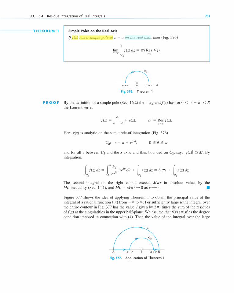
Fig. 377. Application of Theorem 1

a + ra – r a

C2

R

S

–R

T H E O R E M 1 Simple Poles on the Real Axis

If has a simple pole at on the real axis, then (Fig. 376)

limr:0

�C2

f (z) dz � pi Resz�a

f (z).

z � af (z)

SEC. 16.4 Residue Integration of Real Integrals 731

a + ra – r a

C2

x

Fig. 376. Theorem 1

P R O O F By the definition of a simple pole (Sec. 16.2) the integrand has for the Laurent series

Here is analytic on the semicircle of integration (Fig. 376)

and for all z between and the x-axis, and thus bounded on say, Byintegration,

The second integral on the right cannot exceed in absolute value, by theML-inequality (Sec. 14.1), and as

Figure 377 shows the idea of applying Theorem 1 to obtain the principal value of theintegral of a rational function from to . For sufficiently large R the integral overthe entire contour in Fig. 377 has the value J given by times the sum of the residuesof at the singularities in the upper half-plane. We assume that satisfies the degreecondition imposed in connection with (4). Then the value of the integral over the large

f (x)f (z)2pi

���f (x)

�r : 0.ML � Mpr : 0Mpr

�C2

f (z) dz � �

p

0

b1

reiu ireiu du � �

C2

g(z) dz � b1pi � �

C2

g(z) dz.

ƒ g(z) ƒ M.C2,C2

C2: z � a � reiu, 0 u p

g(z)

f (z) �b1

z � a � g(z), b1 � Resz�a

f (z).

0 � ƒ z � a ƒ � Rf (z)

c16.qxd 11/1/10 6:57 PM Page 731

semicircle S approaches 0 as For the integral over (clockwise!)approaches the value

by Theorem 1. Together this shows that the principal value P of the integral from toplus K equals J; hence If has several simple

poles on the real axis, then K will be times the sum of the corresponding residues.Hence the desired formula is

(14)

where the first sum extends over all poles in the upper half-plane and the second over allpoles on the real axis, the latter being simple by assumption.

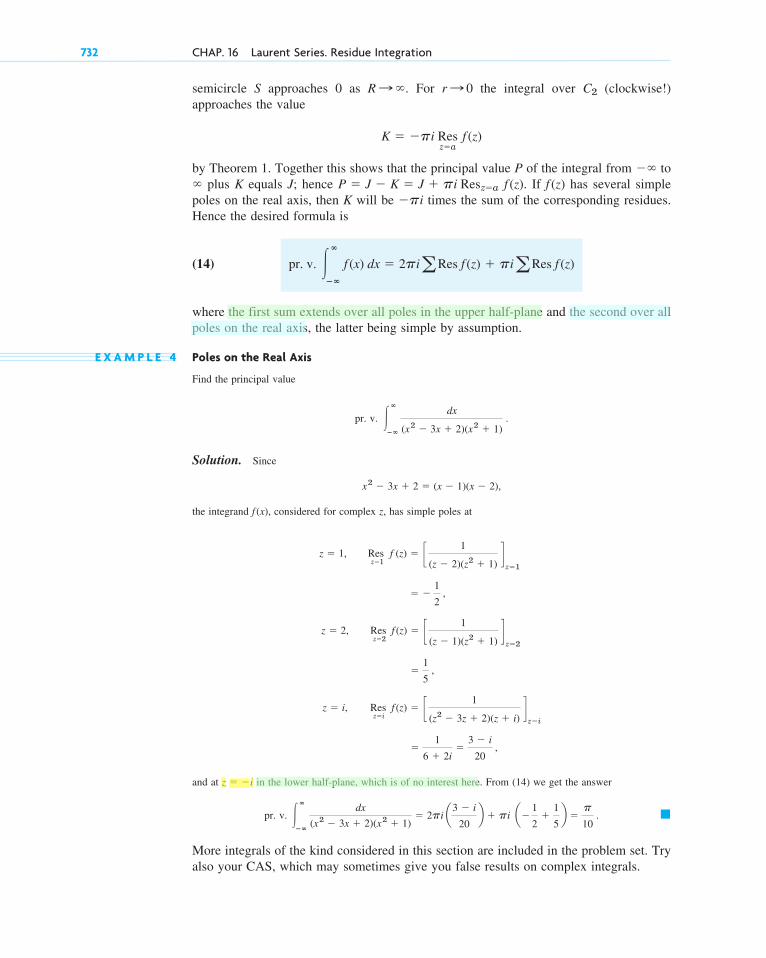
E X A M P L E 4 Poles on the Real Axis

Find the principal value

pr. v.

Solution. Since

the integrand considered for complex z, has simple poles at

and at in the lower half-plane, which is of no interest here. From (14) we get the answer

pr. v.

More integrals of the kind considered in this section are included in the problem set. Tryalso your CAS, which may sometimes give you false results on complex integrals.

���

��

dx

(x2 � 3x � 2)(x2 � 1)� 2pi a3 � i

20 b � pi a�

1

2�

1

5 b �

p

10 .

z � �i

�1

6 � 2i�

3 � i

20 ,

z � i, Res z�i

f (z) � c 1

(z2 � 3z � 2)(z � i) d

z�i

�1

5 ,

z � 2, Res z�2

f (z) � c 1

(z � 1)(z2 � 1) d

z�2

� � 1

2 ,

z � 1, Res z�1

f (z) � c 1

(z � 2)(z2 � 1) d

z�1

f (x),

x2 � 3x � 2 � (x � 1)(x � 2),

��

��

dx

(x2 � 3x � 2)(x2 � 1) .

pr. v. ��

��

f (x) dx � 2piaRes f (z) � piaRes f (z)

�pif (z)P � J � K � J � pi Resz�a f (z).�

��

K � �pi Resz�a

f (z)

C2r : 0R : �.

732 CHAP. 16 Laurent Series. Residue Integration

c16.qxd 11/1/10 6:57 PM Page 732

Chaper 16 Review Questions and Problems 733

1–9 INTEGRALS INVOLVING COSINE AND SINEEvaluate the following integrals and show the details ofyour work.

1. 2.

3. 4.

5. 6.

7. 8.

9.

10–22 IMPROPER INTEGRALS: INFINITE INTERVAL OF INTEGRATION

Evaluate the following integrals and show details of yourwork.

10. 11.

12. 13.

14. 15.

16. 17.

18. 19.

20. ��

��

x

8 � x3 dx

��

��

dx

x4 � 1�

�

��

cos 4x

x4 � 5x2 � 4 dx

��

��

sin 3x

x4 � 1 dx�

�

��

cos 2x

(x2 � 1)2 dx

��

��

x2

x6 � 1 dx�

�

��

x2 � 1

x4 � 1 dx

��

��

x

(x2 � 1)(x2 � 4) dx�

�

��

dx

(x2 � 2x � 5)2

��

��

dx

(1 � x2)2��

��

dx

(1 � x2)3

�2p

0

cos u13 � 12 cos 2u

du

�2p

0

18 � 2 sin u

du�2p

0

aa � sin u

du

�2p

0

sin2 u5 � 4 cos u

du�2p

0

cos2 u

5 � 4 cos u du

�2p

0

1 � 4 cos u17 � 8 cos u

du�2p

0

1 � sin u3 � cos u

du

�p

0

du

p � 3 cos u�p

0

2 du

k � cos u

21.

22.

23–26 IMPROPER INTEGRALS: POLES ON THE REAL AXIS

Find the Cauchy principal value (showing details):

23. 24.

25. 26.

27. CAS EXPERIMENT. Simple Poles on the RealAxis. Experiment with integrals

real andall different, Conjecture that the principal valueof these integrals is 0. Try to prove this for a specialk, say, For general k.

28. TEAM PROJECT. Comments on Real Integrals. (a) Formula (10) follows from (9). Give the details.

(b) Use of auxiliary results. Integrating aroundthe boundary C of the rectangle with vertices

letting and using

show that

(This integral is needed in heat conduction in Sec.12.7.)

(c) Inspection. Solve Probs. 13 and 17 withoutcalculation.

��

0

e�x2

cos 2bx dx �1p

2 e�b2

.

��

0

e�x2

dx �1p

2 ,

a : �,a � ib, �a � ib,�a, a,

e�z2

k � 3.

k 1.f (x) � [(x � a1)(x � a2) Á (x � ak)]�1, aj

���� f (x) dx,

��

��

x2

x4 � 1 dx�

�

��

x � 5

x3 � x dx

��

��

dx

x4 � 3x2 � 4�

�

��

dx

x4 � 1

��

��

dx

x2 � ix

��

��

sin x

(x � 1)(x2 � 4) dx

P R O B L E M S E T 1 6 . 4

1. What is a Laurent series? Its principal part? Its use?Give simple examples.

2. What kind of singularities did we discuss? Give defi-nitions and examples.

3. What is the residue? Its role in integration? Explainmethods to obtain it.

4. Can the residue at a singularity be zero? At a simplepole? Give reason.

5. State the residue theorem and the idea of its proof frommemory.

6. How did we evaluate real integrals by residue integration?How did we obtain the closed paths needed?

C H A P T E R 1 6 R E V I E W Q U E S T I O N S A N D P R O B L E M S

c16.qxd 11/1/10 6:57 PM Page 733

734 CHAP. 16 Laurent Series. Residue Integration

7. What are improper integrals? Their principal value?Why did they occur in this chapter?

8. What do you know about zeros of analytic functions?Give examples.

9. What is the extended complex plane? The Riemannsphere R? Sketch on R.

10. What is an entire function? Can it be analytic atinfinity? Explain the definitions.

11–18 COMPLEX INTEGRALS

Integrate counterclockwise around C. Show the details.

11.

12.

13.

14.

15.25z2

(z � 5)2 , C: ƒ z � 5 ƒ � 1

5z3

z2 � 4 , C: ƒ z � i ƒ � pi>2

5z3

z2 � 4 , C: ƒ z ƒ � 3

e2>z, C: ƒ z � 1 � i ƒ � 2

sin 3z

z2 , C: ƒ z ƒ � p

z � 1 � i

16.

17.

18.

19–25 REAL INTEGRALSEvaluate by the methods of this chapter. Show details.

19. 20.

21.

22. 23.

24. 25. ��

��

cos x

x2 � 1 dx�

�

��

dx

x2 � 4ix

��

��

x

(1 � x2)2 dx�

�

��

dx

1 � 4x4

�2p

0

sin u

34 � 16 sin u du

�2p

0

sin u

3 � cos u du�

2p

0

du

13 � 5 sin u

cot 4z, C: ƒ z ƒ � 34

cos z

zn , n � 0, 1, 2, Á , C: ƒ z ƒ � 1

15z � 9

z3 � 9z , C: ƒ z ƒ � 4

A Laurent series is a series of the form

(1) (Sec. 16.1)

or, more briefly written [but this means the same as (1)!]

where This series converges in an open annulus (ring) A withcenter In A the function is analytic. At points not in A it may havesingularities. The first series in (1) is a power series. In a given annulus, a Laurentseries of is unique, but may have different Laurent series in different annuliwith the same center.

Of particular importance is the Laurent series (1) that converges in a neighborhoodof except at itself, say, for suitable). The series0 � ƒ z � z0 ƒ � R (R 0,z0z0

f (z)f (z)

f (z)z0.n � 0, �1, �2, Á .

f (z) � a�

n���

an(z � z0)n, an �1

2pi �

C

f (z*)

(z* � z0)n�1 dz*(1*)

f (z) � a�

n�0

an(z � z0)n � a�

n�1

bn

(z � z0)n

SUMMARY OF CHAPTER 16Laurent Series. Residue Integration

c16.qxd 11/1/10 6:57 PM Page 734

Summary of Chapter 16 735

(or finite sum) of the negative powers in this Laurent series is called the principalpart of at The coefficient of in this series is called the residueof at and is given by [see (1) and

(2) Thus

can be used for integration as shown in (2) because it can be found from

(3) (Sec. 16.3),

provided has at a pole of order m; by definition this means that principalpart has as its highest negative power. Thus for a simple pole

also,

If the principal part is an infinite series, the singularity of at is called anessential singularity (Sec. 16.2).

Section 16.2 also discusses the extended complex plane, that is, the complex planewith an improper point (“infinity”) attached.

Residue integration may also be used to evaluate certain classes of complicatedreal integrals (Sec. 16.4).

�

z0f (z)

Resz�z0

p(z)

q(z)�

p(z0)

qr(z0) .Res

z�z0 f (z) � lim

z:z0

(z � z0) f (z);

(m � 1),1>(z � z0)mz0f (z)

Resz�z0

f (z) �1

(m � 1)! limz:z0 ¢ dm�1

dzm�1 [(z � z0)mf (z)]≤ ,b1

�C f (z*) dz* � 2pi Res

z�z0 f (z).b1 � Res

z:z0 f (z) �

12pi

�C f (z*) dz*.

(1*)]z0f (z)1>(z � z0)b1z0.f (z)

c16.qxd 11/1/10 6:57 PM Page 735