problem book - .:: · pdf fileproblem book oscar castillo-felisola july 25, 2007. ... iii...

Problem Book

Oscar Castillo-Felisola

July 25, 2007

Contents

I Classical Electrodynamics 11

1 Electrostatics 131.1 Problem. Pr. 1.1 . . . . . . . . . . . . . . . . . . . . . . . . . . . . . . . . . . . . 131.2 Problem. Pr. 1.2 . . . . . . . . . . . . . . . . . . . . . . . . . . . . . . . . . . . . 141.3 Problem. Pr. 1.3 . . . . . . . . . . . . . . . . . . . . . . . . . . . . . . . . . . . . 151.4 Problem. Pr. 1.4 . . . . . . . . . . . . . . . . . . . . . . . . . . . . . . . . . . . . 161.5 Problem. Pr. 1.5 . . . . . . . . . . . . . . . . . . . . . . . . . . . . . . . . . . . . 171.6 Problem. Pr. 1.6 . . . . . . . . . . . . . . . . . . . . . . . . . . . . . . . . . . . . 181.7 Problem. Pr. 1.7 . . . . . . . . . . . . . . . . . . . . . . . . . . . . . . . . . . . . 191.8 Problem. Pr. 1.8 . . . . . . . . . . . . . . . . . . . . . . . . . . . . . . . . . . . . 201.9 Problem. Pr. 1.9 . . . . . . . . . . . . . . . . . . . . . . . . . . . . . . . . . . . . 211.10 Problem. Pr. 1.10 . . . . . . . . . . . . . . . . . . . . . . . . . . . . . . . . . . . 221.11 Problem. Pr. 1.11 . . . . . . . . . . . . . . . . . . . . . . . . . . . . . . . . . . . 231.12 Problem. Pr. 1.12 . . . . . . . . . . . . . . . . . . . . . . . . . . . . . . . . . . . 241.13 Problem. Pr. 1.13 . . . . . . . . . . . . . . . . . . . . . . . . . . . . . . . . . . . 241.14 Problem. Pr. 1.14 . . . . . . . . . . . . . . . . . . . . . . . . . . . . . . . . . . . 25

2 Electrostatic II 272.1 Problem Pr. 2.1 . . . . . . . . . . . . . . . . . . . . . . . . . . . . . . . . . . . . 272.2 Problem Pr. 2.2 . . . . . . . . . . . . . . . . . . . . . . . . . . . . . . . . . . . . 282.3 Problem Pr. 2.3 . . . . . . . . . . . . . . . . . . . . . . . . . . . . . . . . . . . . 292.4 Problem Pr. 2.4 . . . . . . . . . . . . . . . . . . . . . . . . . . . . . . . . . . . . 302.5 Problem Pr. 2.5 . . . . . . . . . . . . . . . . . . . . . . . . . . . . . . . . . . . . 322.6 Problem Pr. 2.6 . . . . . . . . . . . . . . . . . . . . . . . . . . . . . . . . . . . . 332.7 Problem Pr. 2.7 . . . . . . . . . . . . . . . . . . . . . . . . . . . . . . . . . . . . 342.8 Problem Pr. 2.8 . . . . . . . . . . . . . . . . . . . . . . . . . . . . . . . . . . . . 342.9 Additional Problem . . . . . . . . . . . . . . . . . . . . . . . . . . . . . . . . . . 35

3

3 Dielectrics 373.1 Problem Pr. 3.2 . . . . . . . . . . . . . . . . . . . . . . . . . . . . . . . . . . . . 373.2 Problem Pr. 3.3 . . . . . . . . . . . . . . . . . . . . . . . . . . . . . . . . . . . . 393.3 Problem Pr. 3.4 . . . . . . . . . . . . . . . . . . . . . . . . . . . . . . . . . . . . 393.4 Problem Pr. 3.5 . . . . . . . . . . . . . . . . . . . . . . . . . . . . . . . . . . . . 423.5 Problem Pr. 3.6 . . . . . . . . . . . . . . . . . . . . . . . . . . . . . . . . . . . . 433.6 Problem Pr. 3.7 . . . . . . . . . . . . . . . . . . . . . . . . . . . . . . . . . . . . 433.7 Problem Pr. 3.8 . . . . . . . . . . . . . . . . . . . . . . . . . . . . . . . . . . . . 443.8 Problem Pr. 3.9 . . . . . . . . . . . . . . . . . . . . . . . . . . . . . . . . . . . . 453.9 Problem Pr. 3.11 . . . . . . . . . . . . . . . . . . . . . . . . . . . . . . . . . . . 463.10 Problem: Aharanov-Bohm vector potential. . . . . . . . . . . . . . . . . . . . . . 47

4 Electrodynamics I 494.1 Problem Pr. 4.1 . . . . . . . . . . . . . . . . . . . . . . . . . . . . . . . . . . . . 494.2 Problem Pr. 4.2 . . . . . . . . . . . . . . . . . . . . . . . . . . . . . . . . . . . . 514.3 Problem Pr. 4.3 . . . . . . . . . . . . . . . . . . . . . . . . . . . . . . . . . . . . 524.4 Problem Pr. 4.4 . . . . . . . . . . . . . . . . . . . . . . . . . . . . . . . . . . . . 534.5 Problem Pr. 4.5 . . . . . . . . . . . . . . . . . . . . . . . . . . . . . . . . . . . . 544.6 Problem Pr. 4.6 . . . . . . . . . . . . . . . . . . . . . . . . . . . . . . . . . . . . 554.7 Problem Pr. 4.7 . . . . . . . . . . . . . . . . . . . . . . . . . . . . . . . . . . . . 574.8 Problem Pr. 4.8 . . . . . . . . . . . . . . . . . . . . . . . . . . . . . . . . . . . . 584.9 Problem Pr. 4.9 . . . . . . . . . . . . . . . . . . . . . . . . . . . . . . . . . . . . 59

II Quantum Mechanics 61

5 One-dimensional Problems 635.1 Problem 1... . . . . . . . . . . . . . . . . . . . . . . . . . . . . . . . . . . . . . . 635.2 Problem 2... . . . . . . . . . . . . . . . . . . . . . . . . . . . . . . . . . . . . . . 655.3 Problem 3... . . . . . . . . . . . . . . . . . . . . . . . . . . . . . . . . . . . . . . 66

III Thermodynamics and Statistical Mechanics 69

6 Probability 716.1 Problem. Reif 1.1 . . . . . . . . . . . . . . . . . . . . . . . . . . . . . . . . . . . 716.2 Problem. Reif 1.2 . . . . . . . . . . . . . . . . . . . . . . . . . . . . . . . . . . . 716.3 Problem. Reif 1.3 . . . . . . . . . . . . . . . . . . . . . . . . . . . . . . . . . . . 726.4 Problem. Reif 1.4 . . . . . . . . . . . . . . . . . . . . . . . . . . . . . . . . . . . 726.5 Problem. Reif 1.5 . . . . . . . . . . . . . . . . . . . . . . . . . . . . . . . . . . . 726.6 Problem. Reif 1.6 . . . . . . . . . . . . . . . . . . . . . . . . . . . . . . . . . . . 736.7 Problem. Reif 1.7 . . . . . . . . . . . . . . . . . . . . . . . . . . . . . . . . . . . 74

7 Thermodynamics 757.1 Problem. Huang 1-1 . . . . . . . . . . . . . . . . . . . . . . . . . . . . . . . . . . 75

8 Statistical Mechanics 778.1 Problem G.-C. 2.2 . . . . . . . . . . . . . . . . . . . . . . . . . . . . . . . . . . . 778.2 Problem G.-C. 2.5 . . . . . . . . . . . . . . . . . . . . . . . . . . . . . . . . . . . 788.3 Problem G.-C. 2.6 . . . . . . . . . . . . . . . . . . . . . . . . . . . . . . . . . . . 788.4 Problem G.-C. 2.8 . . . . . . . . . . . . . . . . . . . . . . . . . . . . . . . . . . . 798.5 Problem G.-C. 2.10 . . . . . . . . . . . . . . . . . . . . . . . . . . . . . . . . . . 808.6 Problem G.-C. 3.1 . . . . . . . . . . . . . . . . . . . . . . . . . . . . . . . . . . . 818.7 Problem G.-C. 3.2 . . . . . . . . . . . . . . . . . . . . . . . . . . . . . . . . . . . 828.8 Problem G.-C. 3.3 . . . . . . . . . . . . . . . . . . . . . . . . . . . . . . . . . . . 828.9 Problem G.-C. 3.4 . . . . . . . . . . . . . . . . . . . . . . . . . . . . . . . . . . . 848.10 Problem G.-C. 3.5 . . . . . . . . . . . . . . . . . . . . . . . . . . . . . . . . . . . 858.11 Problem G.-C. 3.15 . . . . . . . . . . . . . . . . . . . . . . . . . . . . . . . . . . 868.12 Problem G.-C. 4.3 . . . . . . . . . . . . . . . . . . . . . . . . . . . . . . . . . . . 888.13 Problem G.-C. 4.4 . . . . . . . . . . . . . . . . . . . . . . . . . . . . . . . . . . . 888.14 Problem G.-C. 4.5 . . . . . . . . . . . . . . . . . . . . . . . . . . . . . . . . . . . 898.15 Problem G.-C. 4.8 . . . . . . . . . . . . . . . . . . . . . . . . . . . . . . . . . . . 908.16 Problem G.-C. 5.1 . . . . . . . . . . . . . . . . . . . . . . . . . . . . . . . . . . . 908.17 Problem G.-C. 5.2 . . . . . . . . . . . . . . . . . . . . . . . . . . . . . . . . . . . 918.18 Problem G.-C. 5.3 . . . . . . . . . . . . . . . . . . . . . . . . . . . . . . . . . . . 928.19 Problem G.-C. 5.4 . . . . . . . . . . . . . . . . . . . . . . . . . . . . . . . . . . . 928.20 Problem G.-C. 5.6 . . . . . . . . . . . . . . . . . . . . . . . . . . . . . . . . . . . 938.21 Problem G.-C. 9.1 . . . . . . . . . . . . . . . . . . . . . . . . . . . . . . . . . . . 938.22 Problem G.-C. 9.2 . . . . . . . . . . . . . . . . . . . . . . . . . . . . . . . . . . . 948.23 Problem G.-C. 9.13 . . . . . . . . . . . . . . . . . . . . . . . . . . . . . . . . . . 958.24 Problem G.-C. 9.14 . . . . . . . . . . . . . . . . . . . . . . . . . . . . . . . . . . 958.25 Problem H.6.1 . . . . . . . . . . . . . . . . . . . . . . . . . . . . . . . . . . . . . 968.26 Problem H.6.2 . . . . . . . . . . . . . . . . . . . . . . . . . . . . . . . . . . . . . 978.27 Problem H. 6.4 . . . . . . . . . . . . . . . . . . . . . . . . . . . . . . . . . . . . 988.28 Problem H. 7.1 . . . . . . . . . . . . . . . . . . . . . . . . . . . . . . . . . . . . 99

8.28.1 Canonical Ensamble . . . . . . . . . . . . . . . . . . . . . . . . . . . . . 998.28.2 Grand Canonical Ensable . . . . . . . . . . . . . . . . . . . . . . . . . . . 100

8.29 Problem H. 7.2 . . . . . . . . . . . . . . . . . . . . . . . . . . . . . . . . . . . . 1018.30 Problem H. 7.5 . . . . . . . . . . . . . . . . . . . . . . . . . . . . . . . . . . . . 1018.31 Problem H. 8.2 . . . . . . . . . . . . . . . . . . . . . . . . . . . . . . . . . . . . 102

8.31.1 Ideal Fermi-Dirac Gas . . . . . . . . . . . . . . . . . . . . . . . . . . . . 1038.31.2 Ideal Bose-Einstein Gas . . . . . . . . . . . . . . . . . . . . . . . . . . . 104

8.32 Problem H. 8.3 . . . . . . . . . . . . . . . . . . . . . . . . . . . . . . . . . . . . 1048.33 Problem H. 8.4 . . . . . . . . . . . . . . . . . . . . . . . . . . . . . . . . . . . . 105

9 Special Topics on Statistical Mechanics 1079.1 Problem H. 3.1 . . . . . . . . . . . . . . . . . . . . . . . . . . . . . . . . . . . . 1079.2 Problem H. 3.2 . . . . . . . . . . . . . . . . . . . . . . . . . . . . . . . . . . . . 1079.3 Problem H. 3.3 . . . . . . . . . . . . . . . . . . . . . . . . . . . . . . . . . . . . 1089.4 Problem H. 4.1 . . . . . . . . . . . . . . . . . . . . . . . . . . . . . . . . . . . . 1109.5 Problem H. 4.5 . . . . . . . . . . . . . . . . . . . . . . . . . . . . . . . . . . . . 1119.6 Problem H. 4.6 . . . . . . . . . . . . . . . . . . . . . . . . . . . . . . . . . . . . 1129.7 Problem H. 4.7 . . . . . . . . . . . . . . . . . . . . . . . . . . . . . . . . . . . . 1129.8 Problem H. 4.9 . . . . . . . . . . . . . . . . . . . . . . . . . . . . . . . . . . . . 1139.9 Problem H. 5.1 . . . . . . . . . . . . . . . . . . . . . . . . . . . . . . . . . . . . 1149.10 Problem H. 5.4 . . . . . . . . . . . . . . . . . . . . . . . . . . . . . . . . . . . . 1159.11 Problem H. 9.2 . . . . . . . . . . . . . . . . . . . . . . . . . . . . . . . . . . . . 1189.12 Problem H. 9.3 . . . . . . . . . . . . . . . . . . . . . . . . . . . . . . . . . . . . 1199.13 Problem H. 9.5 . . . . . . . . . . . . . . . . . . . . . . . . . . . . . . . . . . . . 1209.14 Problem H. 11.1 . . . . . . . . . . . . . . . . . . . . . . . . . . . . . . . . . . . . 1219.15 Problem H. 11.2 . . . . . . . . . . . . . . . . . . . . . . . . . . . . . . . . . . . . 1219.16 Problem H. 12.4 . . . . . . . . . . . . . . . . . . . . . . . . . . . . . . . . . . . . 1229.17 Problem H. 14.4 . . . . . . . . . . . . . . . . . . . . . . . . . . . . . . . . . . . . 1229.18 Problem H. 14.5 . . . . . . . . . . . . . . . . . . . . . . . . . . . . . . . . . . . . 1239.19 Problem G.-C. 6.1 . . . . . . . . . . . . . . . . . . . . . . . . . . . . . . . . . . . 1269.20 Problem G.-C. 6.5 . . . . . . . . . . . . . . . . . . . . . . . . . . . . . . . . . . . 1279.21 Problem G.-C. 6.16 . . . . . . . . . . . . . . . . . . . . . . . . . . . . . . . . . . 1289.22 Problem G.-C. 6.17 . . . . . . . . . . . . . . . . . . . . . . . . . . . . . . . . . . 1299.23 Problem G.-C. 7.15 . . . . . . . . . . . . . . . . . . . . . . . . . . . . . . . . . . 1309.24 Problem G.-C. 7.16 . . . . . . . . . . . . . . . . . . . . . . . . . . . . . . . . . . 1319.25 Problem G.-C. 7.20 . . . . . . . . . . . . . . . . . . . . . . . . . . . . . . . . . . 1319.26 Problem G.-C. 7.21 . . . . . . . . . . . . . . . . . . . . . . . . . . . . . . . . . . 1329.27 Problem G.-C. 10.1 . . . . . . . . . . . . . . . . . . . . . . . . . . . . . . . . . . 1329.28 Problem G.-C. 10.2 . . . . . . . . . . . . . . . . . . . . . . . . . . . . . . . . . . 1349.29 Problem G.-C. 10.3 . . . . . . . . . . . . . . . . . . . . . . . . . . . . . . . . . . 1359.30 Problem G.-C. 12.1 . . . . . . . . . . . . . . . . . . . . . . . . . . . . . . . . . . 1379.31 Problem G.-C. 12.2 . . . . . . . . . . . . . . . . . . . . . . . . . . . . . . . . . . 1379.32 Problem G.-C. 12.11 . . . . . . . . . . . . . . . . . . . . . . . . . . . . . . . . . 1389.33 Problem G.-C. 15.1 . . . . . . . . . . . . . . . . . . . . . . . . . . . . . . . . . . 1399.34 Problem G.-C. 15.8 . . . . . . . . . . . . . . . . . . . . . . . . . . . . . . . . . . 140

IV Relativity 141

10 Relativity 14310.1 Problem 1 . . . . . . . . . . . . . . . . . . . . . . . . . . . . . . . . . . . . . . . 14310.2 Problem 2 . . . . . . . . . . . . . . . . . . . . . . . . . . . . . . . . . . . . . . . 145

10.3 Problem 3 . . . . . . . . . . . . . . . . . . . . . . . . . . . . . . . . . . . . . . . 14610.4 Problem 4 . . . . . . . . . . . . . . . . . . . . . . . . . . . . . . . . . . . . . . . 14610.5 Problem 5 . . . . . . . . . . . . . . . . . . . . . . . . . . . . . . . . . . . . . . . 14710.6 Problem 6 . . . . . . . . . . . . . . . . . . . . . . . . . . . . . . . . . . . . . . . 14810.7 Problem 7 . . . . . . . . . . . . . . . . . . . . . . . . . . . . . . . . . . . . . . . 14810.8 Problem 8 . . . . . . . . . . . . . . . . . . . . . . . . . . . . . . . . . . . . . . . 14810.9 Problem 9 . . . . . . . . . . . . . . . . . . . . . . . . . . . . . . . . . . . . . . . 14910.10Problem 10 . . . . . . . . . . . . . . . . . . . . . . . . . . . . . . . . . . . . . . 14910.11Problem 11 . . . . . . . . . . . . . . . . . . . . . . . . . . . . . . . . . . . . . . 14910.12Problem 12 . . . . . . . . . . . . . . . . . . . . . . . . . . . . . . . . . . . . . . 15010.13Problem 13 . . . . . . . . . . . . . . . . . . . . . . . . . . . . . . . . . . . . . . 15110.14Problem 14 . . . . . . . . . . . . . . . . . . . . . . . . . . . . . . . . . . . . . . 15210.15Problem 15 . . . . . . . . . . . . . . . . . . . . . . . . . . . . . . . . . . . . . . 15210.16Problem 16 . . . . . . . . . . . . . . . . . . . . . . . . . . . . . . . . . . . . . . 15410.17Problem 17 . . . . . . . . . . . . . . . . . . . . . . . . . . . . . . . . . . . . . . 15410.18Problem 18 . . . . . . . . . . . . . . . . . . . . . . . . . . . . . . . . . . . . . . 15410.19Problem 19 . . . . . . . . . . . . . . . . . . . . . . . . . . . . . . . . . . . . . . 15510.20Problem 20 . . . . . . . . . . . . . . . . . . . . . . . . . . . . . . . . . . . . . . 15610.21Problem 21 . . . . . . . . . . . . . . . . . . . . . . . . . . . . . . . . . . . . . . 15710.22Problem 22 . . . . . . . . . . . . . . . . . . . . . . . . . . . . . . . . . . . . . . 15710.23Problem 6.10 . . . . . . . . . . . . . . . . . . . . . . . . . . . . . . . . . . . . . 15810.24Problem 6.11 . . . . . . . . . . . . . . . . . . . . . . . . . . . . . . . . . . . . . 15810.25Problem 6.14 . . . . . . . . . . . . . . . . . . . . . . . . . . . . . . . . . . . . . 15910.26Problem 6.17 . . . . . . . . . . . . . . . . . . . . . . . . . . . . . . . . . . . . . 15910.27Problem 6.18 . . . . . . . . . . . . . . . . . . . . . . . . . . . . . . . . . . . . . 16010.28Problem 6.19 . . . . . . . . . . . . . . . . . . . . . . . . . . . . . . . . . . . . . 16110.29Problem 6.20 . . . . . . . . . . . . . . . . . . . . . . . . . . . . . . . . . . . . . 16110.30Problem 6.25 . . . . . . . . . . . . . . . . . . . . . . . . . . . . . . . . . . . . . 161

V Quantum Field Theory 163

11 QFT I 6 16511.1 Problem 1 . . . . . . . . . . . . . . . . . . . . . . . . . . . . . . . . . . . . . . . 16511.2 Problem 2 . . . . . . . . . . . . . . . . . . . . . . . . . . . . . . . . . . . . . . . 16711.3 Problem 3 . . . . . . . . . . . . . . . . . . . . . . . . . . . . . . . . . . . . . . . 168

12 QFT I 7 17112.1 Problem 1 . . . . . . . . . . . . . . . . . . . . . . . . . . . . . . . . . . . . . . . 17112.2 Problem 2 . . . . . . . . . . . . . . . . . . . . . . . . . . . . . . . . . . . . . . . 17312.3 Problem 3 . . . . . . . . . . . . . . . . . . . . . . . . . . . . . . . . . . . . . . . 17512.4 Problem 4 . . . . . . . . . . . . . . . . . . . . . . . . . . . . . . . . . . . . . . . 176

13 Miscellaneous 18113.1 Notation . . . . . . . . . . . . . . . . . . . . . . . . . . . . . . . . . . . . . . . . 18113.2 Gamma matrices in the chiral representation . . . . . . . . . . . . . . . . . . . . . 18113.3 Scalars from Weyl spinors . . . . . . . . . . . . . . . . . . . . . . . . . . . . . . 18213.4 Determinant of a deformation of the identity . . . . . . . . . . . . . . . . . . . . . 18313.5 Lorentz currents for a real scalar field . . . . . . . . . . . . . . . . . . . . . . . . 18413.6 Conservation of the KG inner product . . . . . . . . . . . . . . . . . . . . . . . . 18413.7 Nöther charge for translation . . . . . . . . . . . . . . . . . . . . . . . . . . . . . 18513.8 Spinorial Lagrangian . . . . . . . . . . . . . . . . . . . . . . . . . . . . . . . . . 185

14 Does it need a name? 18714.1 Wick’s Theorem . . . . . . . . . . . . . . . . . . . . . . . . . . . . . . . . . . . . 18714.2 2:2 Scattering in phi3 . . . . . . . . . . . . . . . . . . . . . . . . . . . . . . . . . 18814.3 2:2 Scattering phi4 . . . . . . . . . . . . . . . . . . . . . . . . . . . . . . . . . . 19014.4 Identities for Spinors . . . . . . . . . . . . . . . . . . . . . . . . . . . . . . . . . 19114.5 Dirac Propagator . . . . . . . . . . . . . . . . . . . . . . . . . . . . . . . . . . . 194

15 ... 2nd part 19715.1 Kinematic restrictions for scattering and decay processes . . . . . . . . . . . . . . 19715.2 Bhabha scattering . . . . . . . . . . . . . . . . . . . . . . . . . . . . . . . . . . . 19915.3 Scattering by an external potential . . . . . . . . . . . . . . . . . . . . . . . . . . 20015.4 Feynman rules for a pseudo-scalar mesons theory . . . . . . . . . . . . . . . . . . 202

16 QFT II 3 20516.1 photon-photon Scattering . . . . . . . . . . . . . . . . . . . . . . . . . . . . . . . 20516.2 Rutherford’s scattering . . . . . . . . . . . . . . . . . . . . . . . . . . . . . . . . 20716.3 Crossing symmetry . . . . . . . . . . . . . . . . . . . . . . . . . . . . . . . . . . 209

17 QGT II 4 21317.1 Relativistic form for the flux factor . . . . . . . . . . . . . . . . . . . . . . . . . . 21317.2 Two bodies phase space in the lab frame . . . . . . . . . . . . . . . . . . . . . . . 21317.3 Elastic electron-muon scattering . . . . . . . . . . . . . . . . . . . . . . . . . . . 21417.4 High energy elastic electron-electron scattering . . . . . . . . . . . . . . . . . . . 214

VI Appendixes 217

18 Geometry: Conics 21918.1 Circumference . . . . . . . . . . . . . . . . . . . . . . . . . . . . . . . . . . . . . 21918.2 Ellipse . . . . . . . . . . . . . . . . . . . . . . . . . . . . . . . . . . . . . . . . . 21918.3 Hyperbola . . . . . . . . . . . . . . . . . . . . . . . . . . . . . . . . . . . . . . . 22018.4 Parabola . . . . . . . . . . . . . . . . . . . . . . . . . . . . . . . . . . . . . . . . 22018.5 Conics in polar coordinates . . . . . . . . . . . . . . . . . . . . . . . . . . . . . . 220

19 Special Functions 22119.1 Gamma Function . . . . . . . . . . . . . . . . . . . . . . . . . . . . . . . . . . . 22119.2 Beta Function . . . . . . . . . . . . . . . . . . . . . . . . . . . . . . . . . . . . . 22119.3 Bessel Functions . . . . . . . . . . . . . . . . . . . . . . . . . . . . . . . . . . . 22219.4 Associated Legendre Polynomials . . . . . . . . . . . . . . . . . . . . . . . . . . 22219.5 Hermite Polynomials . . . . . . . . . . . . . . . . . . . . . . . . . . . . . . . . . 22319.6 Laguerre polynomials . . . . . . . . . . . . . . . . . . . . . . . . . . . . . . . . . 223

Bibliography 225

List of Figures 227

List of Tables 229

Part I

Classical Electrodynamics

11

Chapter 1Electrostatics

1.1 Problem. Pr. 1.1A bidimensional electrostatic field varies with x and y. Show that the average of the potential alongany circle is the same that the potential at the center of the circle, bucause there are not charges onthe region.

SolutionConsider a circle centred at the origin of coordinates, the radius is r0. For this set up,

〈Φ〉r0 =1

2πr0

∫r0dθΦ(r0, θ) =

12π

∫dθΦ(r0, θ). (1.1)

Since 〈Φ〉r0 does not depend on r0, it follows that

ddr〈Φ〉r0 = 0. (1.2)

The last equation holds even for r0 → 0, then

〈Φ〉r0 = 〈Φ〉r=0 = Φ(0). (1.3)

If one considers a circle centred at ~R − ~r,

〈Φ〉r0 =1

2πr0

∫r0dθΦ(~R, θ) =

12π

∫dθΦ(~R, θ). (1.4)

Since 〈Φ〉r0 does not depend on r0, it follows that

ddr〈Φ〉r0 = 0. (1.5)

13

The last equation holds even for r0 → 0, then

〈Φ〉r0 = 〈Φ〉r=0 = Φ(~R − ~r). (1.6)

1.2 Problem. Pr. 1.2A piar of parallel infinite plates are separated by a distance s and they are kept at potentials 0 andV0. Use the Poisson equation to finding the potencial on the region between the plates, where thecharge density is ρ = ρ0x/s. The distance x is measured from the grounded plate.What are thesurface charge density on the plates?

SolutionIt’s well known that

∇2V = −ρ

ε0= −

ρ0

ε0sx, (1.7)

then,V = −

ρ0

6ε0sx3 + V ′1x + V1. (1.8)

Since the boundary conditions are V(x = 0) = 0 and V(x = s) = V0, it follows that

V1 = 0. V ′1 =1s

(V0 +

ρ0

6ε0s2

). (1.9)

Finally,

V(x) = −ρ0

6ε0sx3 +

1s

(V0 +

ρ0

6ε0s2

)x. (1.10)

In order to get the charge densities, one can use the result, derived from Gauß’ law,

σi = −ε0∂V∂n

∣∣∣∣∣xi

. (1.11)

Therefore,

σ(x = 0) = −ε0V0

s+ρ0

6s, (1.12)

and

σ(x = s) =ρ0

3s −

ε0V0

s. (1.13)

1.3 Problem. Pr. 1.3The axial electric field Ez on the axis of an accelerated tube in a kind of ionic accelerator is givenby Ez = Ez0 + kz2, where z is measured from the centre of the tube along the axis. The componentEφ is zero. Show that Er = −kzr, assume that the charge density is zero.

Draw the force field.Which is the maximun charge density that can be tolerated if the above radial field has an

accuracy of 5% at the tube extrama? L = 1 m, Ez0 = 7.5 ∗ 105 V/m and k = 106 V/m3.

SolutionSince Ez = Ez0 + kz2 and Eφ = 0, by Gauß’ law, it follows that

~∇ · ~E = 0, (1.14)

so that the set up is considered in the vacuum.In general,

~∇ · ~E =1√

g∂a(√

gEa), (1.15)

then, in cylindric coordinates, it yields

~∇ · ~E =1r∂r(rEe) + ∂φEφ + ∂zEz

=1r∂r(rEr) + ∂zEz. (1.16)

It follows from (1.14) and (1.16) that

1r∂r(rEr) + ∂zEz = 0. (1.17)

Sincer∂zEz = 2kzr, (1.18)

then∂r(rEr) = Er + r∂rEr = −2kzr. (1.19)

Equation (1.19) looks like a Euler differential equation, then one can make and ansatz Er = cr,with c a constant. Substituting into (1.19), one gets

2cr = −2kzr ⇒ c = −kz. (1.20)

Finally,

Er = −kzr. (1.21)

In order to determine the induced chage density at the extrema, up to 5%, the radial electricfield, change to Er → E′r = (1 + 1/20)Er. Therefore,

~∇ · ~E′ =1r∂r(rE′r) + ∂zEz = ∓

kz10=ρin

ε0. (1.22)

At the extrema,

ρ(z = L/2) = ∓kLε0

20, (1.23)

andρ(z = −L/2) = ±

kLε0

20. (1.24)

One just should introduce the numerical values given in the problem,

ρ(z = L/2) = −4.425 ∗ 10−7 Cm3 , (1.25)

ρ(z = −L/2) = 4.425 ∗ 10−7 Cm3 . (1.26)

1.4 Problem. Pr. 1.4A potential V is applied between two coaxil cylinders of radii r1 and r2 respectively. Show that theelectric field has a minimum value when r1 = r2/e.

SolutionBy Gauß’ law, one know that

E(r1 < r < r2) =qin

2πε0rh=σ

ε0

(r1

r

). (1.27)

Since the cylinders are kept to a constant potential, V ,it follows that,

V = −r1σ

ε0

∫ r1

r2

drr= −

σr1

ε0ln

(r1

r2

), (1.28)

therefore,Vr1=σ

ε0ln

(r2

r1

). (1.29)

Next, consider a change on the inner radius, r1 → r1 + ∆r1. Since V is still a constant, thesuperficial charge density must change, σ→ σ′. Then

−V =σr1

ε0ln

(r1

r2

)=σ′r′1ε0

ln(r′1r2

). (1.30)

In roder to see how σ changes with a variation of r1, expand the logaritm

ln(r′1r2

)= ln

(r1

r2

)+∆r1

r1. (1.31)

Inserting the last equation in (1.30), one obtains

σ′

ε0(r1 + ∆r1)

[ln

(r1

r2

)+∆r1

r1

]=

σr1

ε0ln

(r1

r2

),

⇒σ′ − σ

ε0r1 ln

(r1

r2

)+σ′

ε0∆r1

[ln

(r1

r2

)+ 1

]= 0,

⇒ σ = σ′ + σ′∆r1

r1

1 + 1

ln(

r1r2

) . (1.32)

From (1.32) one can obtain the derivative,

dσdr1= lim∆r1→0

σ′ − σ

∆r1= −

1r1

1 + 1

ln(

r1r2

) . (1.33)

In order for ~E been a minimun, (1.33) should be equal to zero, thus,

1 = − ln(r1

r2

)= ln

(r2

r1

)⇒ r1 =

r2

e. (1.34)

1.5 Problem. Pr. 1.5A sheet conductor of arbitrary form carries a charge Q, the density on a region is σ. Gauß’ lawstates that just out of the surface the electric field is σ/ε0. Show that if a small hole is made, theelectric field at the hole is σ/2ε0.

SolutionGauß’ law states ∮

S

~dS · ~E =qin

ε0. (1.35)

In the inner space of a conductor, the electric field vanishes, so by (1.35), one gets

E ∗ A =σAε0

⇒ E =σ

ε0. (1.36)

Nonetheless, if a small hole is made on the conductor, due to the linear property of the equa-tions, the new set up can be realized like a conductor with charge density σ plus a disk with charge

density −σ. When the electric field ~E is measure at a distance d → 0 from the disk, it seems to bean infinite plate therefore,

E′ ∗ 2A = −σAε0

⇒ E′ = −σ

2ε0. (1.37)

Hence,

Et = E + E′ =σ

2ε0. (1.38)

1.6 Problem. Pr. 1.6Calculate the dipolar momentum of a spherical sheet with a charge density σ = σ0 cos θ, with θ isthe polar angle.

SolutionIt’s well known that the dipolar momentum is given by

~p =∫

V′d3x′ ~x′ρ(x′). (1.39)

Since the considered configuration is

σ = σ0 cos θ, ⇒ ρ = σ0 cos θδ(r − a)

a2 . (1.40)

Then,

px = aσ0

∫ π

0

∫ 2π

0sin θdθdϕ sin θ cosϕ cos θ

= 0 (1.41)

py = aσ0

∫ π

0

∫ 2π

0sin θdθdϕ sin θ sinϕ cos θ

= 0 (1.42)

pz = 2πaσ0

∫ π

0sin θdθ cos θ cos θ

= −2πaσ0

∫ π

0d(cos θ) cos2 θ

= −23πaσ0(−1 − 1)

=43πaσ0. (1.43)

From eqs. (1.41),(1.42) and (1.43), one finally obtains,

~p =43πaσ0k. (1.44)

1.7 Problem. Pr. 1.7Find the required time for a pair of plate of a plane capacitor join, if the mass density is m0 andthey are separated by an initial distance x0.

1. When the plates are charged with a density σ and then isolated.

2. When the plates are kept to a constant potential V .

SolutionA pair of charged plane (and infinete) plates are considered. Assume the charge density is σ, andtheir mass by unit area is m0.

Hence, on a characteristic area element,

d ~F = dq~E, (1.45)

with ~E the electric field generated by the opposite plate.From (1.35) and (1.37), (1.45) can be written like

d ~F = dqσ

2ε0= −

σ2a2

2ε0= m0a2 x. (1.46)

Now, by kinematics,

~x0 = −12

at2. (1.47)

Thus,

t =

√−

2x0

x

=2σ

√x0m0ε0. (1.48)

On the other hand, if one id interested on a couple of plates kept at constant potential, on mustconsider the change of the capacitance.

C =qV=ε0Ad, (1.49)

i.e.,

σ(x) =qA=ε0V0

x. (1.50)

By Gauß’ law,~E =

σ

2ε0=

V0

x. (1.51)

Hence,

d ~F = −a2V2

0 ε0

2x2 = m0a2 x, (1.52)

then,

m0 xx = −V2

0 ε0

2xx2 , (1.53)

thus,ddt

(m0 x2 −

V20 ε0

x

)= 0. (1.54)

This yields,

dxdt=

√V2

0 ε0

m0

(1x+ c

). (1.55)

Since x(t = 0) = 0 at x(t = 0) = x0,

dxdt=

√V2

0 ε0

m0

(1x+

1x0

)=

√V2

0 ε0

m0x0

( x0 − xx

), (1.56)

Therefore, ∫ 0

x0

dx√

x√

x0 −√

x=

√V2

0 ε0

m0x0t. (1.57)

Changing√

x = −√

x0 sin θ,∫ 0

x0

dx√

x√

x0 −√

x= 2x0

∫ π/2

0dθ sin2 θ = x0

(π

2+ 1

), (1.58)

Thus,

t = x0

(π

2+ 1

) √m0x0

ε0V20

. (1.59)

1.8 Problem. Pr. 1.8A variable capacitor consists on a couple of coaxial cylinders of radii a and b with b− a << a, freeof moving along the coaxial direction. Use energy methods to calculate the magnitud and directionof the force on the inner cylinder if it’s displaced respect the exterior cylinder.

SolutionThe energy carried by a capacitor is

U =q2

2C, (1.60)

with q the charge on the capacitor and C its capacitance.For a cylinder capacitor,

C =2πε0L

ln(b/a). (1.61)

If one moves the inner cylinder a distance x, the effective cylinder capacitor has length L − x, thus

C(x) =2πε0(L − x)

ln(b/a). (1.62)

Moreover, the force on that cylinder is given by

~F = −~∇U

= −q2

4πε0ln

(ba

)x

(L − x)2 . (1.63)

1.9 Problem. Pr. 1.9Verify that the charge on a grounded infinite conductive plane, induced by a point charge, q at adistance a from the plane, is −q.

SolutionBy the image method, the position of the image charge is (−a, 0, 0) and its charge is −q,becauseΦ(0, y, z) = 0. Moreover,

Φ(x, y, z) =q

4πε0

1√(x − a)2 + y2 + z2

−1√

(x + a)2 + y2 + z2

. (1.64)

From Gauß’ law, ∮S

~E · d~S = −

∮S

~∇Φ · ndS

= −

∮S

∂Φ

∂ndS

=σSε0, (1.65)

then,

σS = −ε0∂Φ

∂n

∣∣∣∣∣S. (1.66)

Finally,σ(x = 0) = −

qa2π(a2 + y2 + z2)3/2 . (1.67)

Hence,

qt =

∫dydxσ(y, z)

= −qa2π

∫rdrdθ

1(a2 + r2)3/2

= −qa∫

rdr(a2 + r2)3/2

= qa(

1(a2 + r2)1/2

)∣∣∣∣∣∣∞0

= −q. (1.68)

1.10 Problem. Pr. 1.10Find Φ(~r) generated by a point charge, q, placed at a distance d from a conducting sphere of radiusR.

SolutionSince the set up has axial symmetry, the image charge must life on the axis that joins the centerof the sphere with the charge q. Consider the image charge,−q′, placed at a distance d′ from thecenter.

By definition of conductor, Φ|S = 0. The most straightforware of getting this condition on thesphere is applying for the points colineals with the axis. Then,

q4πε0

1d − R

=q′

4πε0

1R − d′

⇒q

4πε0d1

1 − R/d=

q′

4πε0R1

1 − d′/R, (1.69)

in order to hold the equality,

q′ = qRd

(1.70)

d′ =R2

d. (1.71)

1.11 Problem. Pr. 1.11Consider a fluid conduct of rectangular form, delimited by the plane points, (0, 0), (a, 0), (0, b) and(a, b). The edges of the rectangle are a constant temperature T1 and T2 and the front edges haveequal temperature. Find the temperature, T (x, y), for all point inside the conduct.

SolutionConsider the Laplacian equation in rectangular coordinates,

∇2T = 0. (1.72)

One can consider homogeneous boundary conditions at x = 0 and x = a. After the separationof variables,

X′′ + m2X = 0 ⇒ X = Am cos mx + Bm sin mx, (1.73)Y ′′ − m2Y = 0 ⇒ Y = Cm cosh my + Dm sinh my, (1.74)

with m > 0. By the boundary condition,

X(x) = Bn sinnπx

a

Y(x) = Dn sinhnπ(y − b)

a, (1.75)

or

X(x) = Bn sinnπx

aY(x) = Dn sinh

nπya, (1.76)

where n = maπ

. (1.75) for homogeneous B.C. at y = b and (1.76) for homogeneous B.C. at y = 0.One can consider homogeneous boundary conditions at y = 0 and y = b. After the separation

of variables,

Y ′′ + m2Y = 0 ⇒ Y = Am cos my + Bm sin my, (1.77)X′′ − m2X = 0 ⇒ X = Cm cosh mx + Dm sinh mx, (1.78)

with m > 0. By the boundary condition,

Y(x) = Bn sinnπyb

X(x) = Dn sinhnπ(x − a)

b, (1.79)

or

Y(x) = Bn sinnπyb

X(x) = Dn sinhnπx

b, (1.80)

where n = maπ

. (1.79) for homogeneous B.C. at x = a and (1.80) for homogeneous B.C. at x = 0.By using the relations ∫ a

0dx sin2 nπx

a=

a2, (1.81)

∫ a

0dx sin

nπxa= −

anπ

((−1)n − 1), (1.82)

and the linelity of the Laplace equation, the coordinate temperature is

T (x, y) = −4T1

π

∑n odd

1n

sin nπxa

sinh nπba

(sinh

nπa

(y − b) + sinhnπa

y)

= −4T2

π

∑n odd

1n

sin nπyb

sinh nπab

(sinh

nπb

(x − a) + sinhnπb

x). (1.83)

1.12 Problem. Pr. 1.12The one of the Bridge...

Solution

1.13 Problem. Pr. 1.13Verify that φ satisfies the Laplace eq. by using the chain rule.

SolutionOne begins with the Laplacian equation

∇2φ = 0. (1.84)

If one would like to change (x, y) to (u, v) coordinates with u = u(x, y) and v = v(x, y) given by thereal and imaginary part of an analytic function, i.e., each of them satisfy the Laplace equation onthe (x, y) coordinates.

By the chain rule, it follows that,

φxx = φuuxx + φvvxx + φuuu2x + φvvv2

x + 2φuvuxvx, (1.85)φyy = φuuyy + φvvyy + φuuu2

y + φvvv2y + 2φuvuyvy, (1.86)

Then, adding both terms,

0 = φu∇2(x,y)u + φv∇

2(x,y)v + φuu(u2

x + u2y) + φvv(v2

x + v2y). (1.87)

Next, one uses the Cauchy equations

ux = vy, (1.88)uy = −vx, (1.89)

then, by changing vx and vy by u’s, (1.87) becomes

0 = (φuu + φvv)(u2x + u2

y). (1.90)

Since ux and uy are not vanishing quantities, it follows that(∂2

∂u2 +∂2

∂v2

)φ(u, v) = 0. (1.91)

1.14 Problem. Pr. 1.14How do ~p and Qi j transform under a traslation on the coordinate system?

SolutionBy definition,

pi =

∫V

riρ(~r)d3r, (1.92)

andQi j =

∫V

d3rρ(~r)(3xix j − δi j~r2). (1.93)

Under r 7→ r′ = r + a,

pi 7→ p′i =∫

Vr′iρ(~r′)d3r′ =

∫V

(ri + ai)ρ(~r′)d3r′

= pi + aiqt, (1.94)

where ∫V

riρ(~r′)d3r′ = pi,

∫V

(ri + ai)ρ(~r′)d3r′ = qt. (1.95)

This happens because V is the volume where the charge density is placed.Similarly,

Qi j 7→ Q′i j =

∫V

d3r′ρ(~r′)(3x′i x′j − δi j~r′

2)

=

∫V

d3rρ(~r)(3(xi + ai)(x j + a j) − δi j(~r + ~a)2

)=

∫V

d3rρ(~r)(3(xix j + xia j + aix j + aia j) − δi j(~r2 + 2~r · ~a + ~a2)

)= Qi j + 3(ai p j + a j pi) + qt(3aia j + ~a2δi j). (1.96)

Chapter 2Electrostatic II

2.1 Problem Pr. 2.1

The energy of a dipole p in a field ~E is W = −~p · ~E. Use the method of images to find the energyof a dipole p at a distance r from an infinite, grounded, conducting plane when the angle betweenp and the normal to the plane is θ.

Find the force and torque on the dipole due to the induced charges on the plane.

Solution

The electric field prodeced by a dipole is

~E(~r) =q

4πε0

~r + ~r′ + ~l|~r + ~r′ + ~l|3

−~r + ~r′

|~r + ~r′|3

. (2.1)

By expanding the denominator,

|~r + ~r′ + ~l|−3 = |~r + ~r′|−3

1 + 3(~r − ~r′) · ~l|~r + ~r′|2

+ . . .

, (2.2)

then,

~E(~r) =1

4πε0

(3

(~r − ~r′) · ~p|~r + ~r′|5

(~r − ~r′) −~p

|~r + ~r′|3

). (2.3)

Putting ~r′ = 0, ~r = −2ri and ~p = −p(cos θi+ sin θ j), the electric field due to the image dipole at theposition of the dipole is

~Eext =p

32πε0r3 (−2 cos θi + sin θ j). (2.4)

27

Since W = −~p · ~Eext and ~p = p(− cos θi + sin θ j), it follows that

W = −p2

32πε0r3 (1 + cos2 θ). (2.5)

Since the net charge is zero, and the dipoles are punctuals, there isn’t net force.

~F = 0. (2.6)

2.2 Problem Pr. 2.2Show that a harmonic function F is uniquely determined at all the points within a given region byits value at the boundary.

Show also that F if identically equal to zero throughout the region if it vanishes at all points ofits boundary.

SolutionIn order to show that the solution is unique, assume that there exist two different functions F1 andF2 s.t. both satisfy the B.C. Fi|S = Fs.

Since the Laplace equation is linear, the function F = F1 − F2 satisfies ∇2F = 0 with homoge-neous B.C.

The Green’s identity states that∫S

u~∇v · d~σ =∫

V(u∇2v + ~∇u · ~∇v)dτ. (2.7)

For the case u = v = F, since F|S = 0 and ∇2F = 0, Green’sidentity yields∫V

(~∇F)2dτ = 0. (2.8)

This implies that ~∇F = 0 and then, F1 = F2 + const. but the B.C. implies that const = 0, i.e.,

F1 = F2.

Moreover, since the solution of the Laplace equation with constant boundary conditions cannothave maxima or minima inside the boundary,it follows that if F|S = 0, then

F|V = 0 .

2.3 Problem Pr. 2.3A small hemispherical bump, of radius a, is raised on the inner surface of one plate of a parallel-plate capacitor, separated by a distance d. Find the resulting potential between the plates.

SolutionIn order to solve the problem, one sholud solve the Laplace equation inside the capacitor. Note thatthe problem has azimutal symmetry, then

Φ(r, θ) = A0 +

∞∑l=1

(Alrl + Blr−(l+1)

)Pl(cos θ). (2.9)

the coefficient B0 = 0 because the innersolution is regular and the logarithmic part of the solutionis dropped.

The boundary conditions are

Φ(r = a) = Φ0, (2.10)Φ(θ = π/2) = Φ0, (2.11)

Φ(r = d/ cos θ) = 0, (2.12)

Φ(r >> a) =σ

ε0cos θ.. (2.13)

Then, by finiteness, Al>1 = 0, also equation (2.13) the coefficients A1 =σε0

and B1 are the onlyones allowed, ’ceuse P1(cos θ) = cos θ. Then

Φ(r, θ) = A0 +σ

ε0r cos θ +

B1

r2 cos θ. (2.14)

From (2.11),

Φ(θ = π/2) = A0 = Φ0, ⇒ Φ(r, θ) = Φ0 +σ

ε0r cos θ +

B1

r2 cos θ. (2.15)

From (2.10),

Φ(a, θ) = Φ0 +

(σaε0+

B1

a2

)cos θ = Φ0, (2.16)

thus,

B1 = −σa3

ε0⇒ Φ(r, θ) = Φ0 +

(σ

ε0r −

σa3

ε0r2

)cos θ. (2.17)

Finally, condition (2.12) yields

Φ(r = d/ cos θ) = Φ0 +σ

ε0

(d −

a3

d2 cos3 θ

)= 0, (2.18)

then, since a << d,

σ = −Φ0ε0

d. (2.19)

Therefore,

Φ(r, θ) = Φ0

(1 +

r3 − a3

r2dcos θ

). (2.20)

2.4 Problem Pr. 2.4A charge Q is uniformly distributed throughout the volume of an ellipsoid of revolution whosesemi-major axis is a and whose semi-minor axis is b. Find the electrostatic potential at any in thespace outside the ellipsoid.

SolutionThe most useful coordinate system for solving the problem is cylindric coordinates. Then, thepotential due to a differential of volume is

dΦ(h) =ρ

4πε0

rdrdθdz√r2 + (h − z)2

, (2.21)

the potential of the ellipsoid is therefore,

Φ(h) =ρ

4πε0

∫ 2π

0dθ

∫ a

−adz

∫ R

0

rdr√r2 + (h − z)2

, (2.22)

with

R2 = b2(1 −

z2

a2

). (2.23)

Then, (2.22) yields,

Φ(h) =ρ

2ε0

∫ a

−adz

( √R2 + (h − z)2 − h + z

). (2.24)

Call I and II the first and second integral of the RHS of (2.24),then,

II =∫ a

−a(−h + z) = −2ah. (2.25)

The argument of the square-root of I can be written asz√

1 −b2

a2 −h√

1 − b2

a2

2

+ b2 + h2 −h2a2

a2 − b2 . (2.26)

After defining

u = z

√1 −

b2

a2 −h√

1 − b2

a2

, J2 = b2 + h2 −h2a2

a2 − b2 , (2.27)

one can change the integral on z by an integral on u, with

du = dz

√1 −

b2

a2 ,

thus,

I =1√

1 − b2

a2

∫ u+

u−du√

u2 + J2

=1√

1 − b2

a2

u√

u2 + J2

2+

J2

2ln(u +

√u2 + J2)

∣∣∣∣∣∣∣u+

u−

. (2.28)

On the above equations, the integration limits are

u+ = a

√1 −

b2

a2 −h√

1 − b2

a2

(2.29)

u− = −a

√1 −

b2

a2 −h√

1 − b2

a2

(2.30)

After a lot of algebraic manipulation, one gets

I =1√

1 − b2

a2

[h(b2 − 3a2 −

h2a2

a2 − b2

)(2.31)

+(b2 + h2)(a2 − b2) − h2a2

2(a2 − b2)ln

((a2 − b2)2 + a(a2 − b2) + h(ha2 − 2a3 + 2ab2 − a2 + b2)(a2 − b2)2 + a(a2 − b2) + h(ha2 + 2a3 − 2ab2 + a2 − b2)

)].

Finally, the potential on the z axis is

Φ =ρ

2ε0

−2ah +1√

1 − b2

a2

[h(b2 − 3a2 −

h2a2

a2 − b2

)(2.32)

+(b2 + h2)(a2 − b2) − h2a2

2(a2 − b2)ln

((a2 − b2)2 + a(a2 − b2) + h(ha2 − 2a3 + 2ab2 − a2 + b2)(a2 − b2)2 + a(a2 − b2) + h(ha2 + 2a3 − 2ab2 + a2 − b2)

)].

2.5 Problem Pr. 2.5Find the potential distribution inside a hollow conducting cylinder of radius a if the cylinder has alength L and the two ends are closed by plates which are held at the potentials Φ = Φ0 and Φ = 0,respectively. Also find the charge distribution on the surface of the cylinder.

SolutionIn order to find the potential, one must solve the Laplace equation with the given boundary condi-tions,

Φ(z = 0) = 0, (2.33)Φ(z = L) = Φ0, (2.34)Φ(r = a) = Φ1. (2.35)

Using cylindric coordinates, it follows that

Φ(ρ, θ, z) = f (ρ)g(θ)h(z), (2.36)

with

f (ρ) = Jm(kρ), (2.37)g(θ) = Am sin(mθ) + Bm cos(mθ), (2.38)h(z) = sinh(kz), (2.39)

with m ∈ Z.For having a well-possed problem, i.e., determine completely all the arbitrary constants, Φ1 =

0, then

Jm(ka) = 0,→ k =λ(m)

n

a, (2.40)

with n ∈ N and λ(m)n is the n-th zero of the m-th Bessel function.

Moreover, due to the azimutal symmetry, m = 0, then

Φ(ρ, θ, z) =∞∑

n=1

An sinh(λ(0)

n

az)

Jm

(λ(0)

n

aρ

). (2.41)

Now, by (2.34) and the identities∫ a

0dρρJn(xnmx/a)Jn(xnm′ x/a) =

a2

2Jn+1(xnm)δmm′ , (2.42)∫ 2π

0sin2 x = π, (2.43)

Figure 2.1: It shows the Bessel functions J0 (in blue) and J1 (in red).

it follows that

An =2a2

Φ0cosech(λ(0)n L/a)

J21(λ(0)

n )

∫ a

0dρρJ0(λ(0)

n ρ/a). (2.44)

Since, ∫dρρnJn−1(ρ) = ρnJn(ρ), (2.45)

and Jn>1(ρ = 0) = 0, the coefficients are

An =2Φ0

λ(0)n

cosech(λ(0)n L/a)

J1(λ(0)n )

. (2.46)

Finally,

Φ(ρ, θ, z) =∞∑

n=1

2Φ0

λ(0)n

cosech(λ(0)n L/a)

J1(λ(0)n )

sinh(λ(0)

n

az)

Jm

(λ(0)

n

aρ

). (2.47)

2.6 Problem Pr. 2.6

A spherical distribution of radius R and constant charge density ρ contains a hole of radius r inside.Determine energy of this configuration.

Solution

2.7 Problem Pr. 2.7Calculate the exterior potential of a infinite, conducting cylinder of radius R on a uniform electricfield E0perpendicular to the axis of it.

SolutionSince the cylinder is infinite, the problem is nothing but 2-dimensional, so, the general solution is

Φ(r, θ) = A0 + B0 ln r +∑

n

(AnrnBnr−n)(Cn sin(nθ) + Dn cos(nθ)). (2.48)

The B.C. are~E(r → ∞) = E0k, (2.49)

⇒ Φ(r → ∞) = −E0r cos θ + const. (2.50)Φ(r = R) = Φ0. (2.51)

At r → ∞, the B.C.implies

Φ(r, θ) = A0 + A1r cos θ +B1

rcos θ = −E0r cos θ + const., (2.52)

thenA1 = −E0.

At r = R, the B.C. implies,

Φ(R, θ) = A0 − E0r cos θ +B1

rcos θ = Φ0, (2.53)

then,A0 = Φ0 B1 = E0R2.

Finally,

Φ(r, θ) = Φ0 − E0R(1 −

Rr

)cos θ. (2.54)

2.8 Problem Pr. 2.8Find the corrents and equipotential of a cylinder, of radius a immerced on a fluid. For that use aconformal map given by

z = ζ +a2

ζ, (2.55)

with ζ = ξ + ıη is the complexification of the original variales (ξ, η) and z = x + ıy is the complexi-fication of the maped coordinates.

SolutionSince ζ = ξ + ıη,

x + ıy = ξ + ıη +a2

ξ2 + η2 (ξ − ıη), (2.56)

then,

x = ξ

(1 +

a2

ξ2 + η2

), (2.57)

y = η

(1 +

a2

ξ2 + η2

). (2.58)

The conformal map maps the B.C. at infinity to the same condition but in the z-plane, but thecircle is maped to a segment on the x axis. Thus, the velocity in the xy-plane is ~v = vx or Φ = vx.

From (2.57), it follows that

Φ = vξ(1 +

a2

ξ2 + η2

). (2.59)

So that this is a conformal map, all the machinany of the complex variable applies, so, the Cauchyconditions imply that

Ψ = vy = vη(1 +

a2

ξ2 + η2

), (2.60)

are the perpendicular lines to Φ.Φ gives the currents, and Ψ gives the equipotentials.

2.9 Additional ProblemFind a relatioin between the multipoles expansion and the Legendre polynomial, of course for anaxial charge distribution.

SolutionThe outside solution of electric potentials with azimutal symmetry can be written as

Φ(r, θ) =∞∑

l=0

Bl

rl+1

=1

4πε0

(Qt

r+

p cos θr2 +

12r5 Qi jxix j + . . .

)(2.61)

For a symmetric configuration the quadrupolar tensor is given by

[Q] =

Q 0 00 Q 00 0 −2Q

, (2.62)

thus,Qi jxix j = Qr2(1 − 3 cos2 θ) = −2Qr2P1(cos θ). (2.63)

Therefore, by comparison,

B0 =Qt

4πε0, B1 =

p4πε0

, B2 = −Q

4πε0. (2.64)

Chapter 3Dielectrics

3.1 Problem Pr. 3.2

A holed dielectric sphere with inner and outer radii a and 2a rspectively, and dielectric coefficientKe = 3, is placed in a previously uniform electric field E0.Show that in the hole

~E =2734

~E0. (3.1)

Solution

The problem has azymutal symmetry, so, as there aren’t free charges, the potential solves theLaplace eq. ∇2φ = 0. Therefore, the solution can be expand in Legendre polynomials.

Call

φi(~r) If r < aφm(~r) If a < r < 2aφe(~r) If r > 2a. (3.2)

Since the potential is continuous, the B.C. are

B.C. r = a

φi(a) = φm(a), (3.3)

ε0∂φi

∂r(a) = ε

∂φm

∂r(a). (3.4)

37

B.C. r = 2a

φe(2a) = φm(2a), (3.5)

ε0∂φe

∂r(2a) = ε

∂φm

∂r(2a). (3.6)

Due to finiteness of the potential for r → 0 or r → ∞, it follows that,

φi =∑

l

AlrlPl(cos θ) (3.7)

φm =∑

l

(Blrl +

Cl

rl+1

)Pl(cos θ) (3.8)

φe = −E0r cos θ +∑

l

Dl1

rl+1 Pl(cos θ). (3.9)

Then, the B.C. are clearly not compatible, unless l = 1, therefore,Continuity r = a

A1a = B1a +C1

a2 , (3.10)

Gauß r = a

ε0A1 = ε(B1 − 2

C1

a3

), (3.11)

Continuity r = 2a

−2aE0 +D1

4a2 = 2aB1 +C1

4a2 , (3.12)

Gauß r = 2a

ε0

(−E0 −

D1

4a2

)= ε

(B1 − 2

C1

a3

). (3.13)

The system of equations (3.10)-(3.13) can be solved, and yield

A1 = −2734

E0, (3.14)

B1 = −2134

E0, (3.15)

C1 = −3a3

17E0, (3.16)

D1 =49a3

17E0. (3.17)

In the hole, one needs just the value of A1, so

φi(r, θ) = −2734

E0r cos θ = −2734

E0z, (3.18)

thus,

~Ei = −~∇φi =2734

~E0. (3.19)

3.2 Problem Pr. 3.3

Use Biot-Savart law for calculating ~B in the center of a square loop carrying a current I.

Solution

Boit-Savart law states

~B =I

4πε0c2

∮ ~dl × ~r|~r|3

. (3.20)

For a square loop, the total contribution in the center is four times the contributions of a single side,so

d~B =Ia

4πε0c2 k∫ a

−a

dl√

a2 + l23. (3.21)

By a trigonometric change, the integral can be solved then one multiply by 4, and the result is

~B =√

2Ia

πε0c2 k. (3.22)

3.3 Problem Pr. 3.4

A plane conductor of width 2a carries a current I. Show that

Bx = −µ0I4πa

θ (3.23)

Bx =µ0I4πa

lnr2

r1(3.24)

in the first coordinate quarter. The conductor’s borders are placed at x = ±a, the current flows indirection z. r1,2 are the distances between x = ±a and the point where the measure is made. Theangle θ is the one between r1 and r2 measure in the direction 1→ 2.

Compute ~B at 26cm from the center of the conductor for an angle of 72o if the conductor bandhas 10cm of width and carries a current of 5.76A.

Find ~B at a distace D, from the origin, placed on the axis x and y. Compare both results forD a.

SolutionTheough the problem the angles between r1 and r2 w.r.t. the x axis are called α and ϕ. Also, theangle of an arbitrary point placed on the conductor is called ϑ, and the modulus (from there to themeasure point) is d.

Begin by consider the magnetic field produced by an infinitesimal wire composing the conduct-ing band, so,

dx = r1 cosα − x = d cosϑ, (3.25)dy = r1 sinα = d sinϑ, (3.26)d2 = d2

x + d2y . (3.27)

Similarly,

Bx = −B sinϑ, (3.28)By = B cosϑ, (3.29)

where, by Amperè’s law,

B =µ0I4πa

dxd. (3.30)

Therefore, the total magnetic field components are

Bx = −µ0Ir1 sinα

4πa

∫ a

−a

dx(r2

1 sin2 α + (r1 cosα − x)2) , (3.31)

By =µ0I4πa

∫ a

−a

(r1 cosα − x)dx(r2

1 sin2 α + (r1 cosα − x)2) . (3.32)

Consider the integral on (3.31),∫ a

−a

dx(r2

1 sin2 α + (r1 cosα − x)2) = 1

r21 sin2 α

∫ a

−a

dx1 + (r1 cosα − x

r1 sinα

)2 , (3.33)

by changingu =

r1 cosα − xr1 sinα

, (3.34)

the integral is solved∫ a

−a

dx(r2

1 sin2 α + (r1 cosα − x)2) = − 1

r1 sinα[arctan(u(a)) − arctan(u(−a))] , (3.35)

withu(±a) =

r1 cosα ∓ ar1 sinα

. (3.36)

Thus

Bx =µ0I4πa

[arctan(u(a)) − arctan(u(−a))] . (3.37)

Since r1 sinα = r2 sinϕ and ϕ + θ = α, it follows that

u(a) = tanϕ, (3.38)u(−a) = tanα, (3.39)

So,

∴ Bx =µ0I4πa

θ. (3.40)

The integral (3.32) is made through the change u = r21 sin2 α + (r1 cosα − x)2, and using the

substitutions u(a) = r21 and u(−a) = r2

2. So

By =µ0I4πa

lnr2

r1. (3.41)

For the given data, the corresponding radii and angles are

α = 86.05r1 = 0.2517 mϕ = 64.96r2 = 0.2771 mθ = 21.09= 0.368 rad

Thus,

Bx = −4.24 ∗ 10−6N/mBy = 1.11 ∗ 10−6N/mB = 4.38 ∗ 10−6N/m

On the x axis,

Bx = 0, (3.42)

By =µ0I4πa

ln(1 +

2aD

). (3.43)

On the y axis,

Bx = −µ0I4πa

2 arctan( aD

), (3.44)

By = 0. (3.45)

By expanding to first order on a, i.e. D a,

ln(1 + x) = x + · · · (3.46)arctan x = x + · · · , (3.47)

one obtains,

|Ba| = |Bb| =µ0IπD

. (3.48)

This is ’cause for D a, the band looks like a wike.

3.4 Problem Pr. 3.5A pair of Helmholtz coils consist in a pair of identical coaxial circle loops,they maximize ~B’suniformity in the intediate region. Find the optimal separation between the loops.

SolutionFor a single loop,

~B(z) =µ0I2

R2(R2 + z2)3/2 , (3.49)

thus, on the Helmholtz coils,

~B(z) =µ0I2

R2

1(R2 + z2)3/2 +

1(R2 +

(z − d

2

)2)3/2

. (3.50)

From the last equation, it follows that

∂~B∂z

(d2

)= 0. (3.51)

It’s not a bad result, but still does not give a relation between the radii and separation of the coils.By taking the second derivative one get

∂2~B∂z2

(d2

)∝

− 6R2(R2 +

(d2

)2)7/2 +

4(R2 +

(d2

)2)5/2 +

4(

d2

)2(R2 +

(d2

)2)7/2

, (3.52)

hence, in order to maximize the uniformity of ~B it must vanish, so the condition reached is

R = d. (3.53)

3.5 Problem Pr. 3.6Find ~B inside a long straight wire of radius a carrying a current density ~J. Assume the electrondensity through the wire is N and their velocity is ~u, find the direction and magnitud of the forceacting on the movil charges. Is the assuption of a uniform charge density realistic?

SolutionAssuming that the current density is uniform, allows using the eq∮

~B · ~dl =Ienc

ε0c2 , (3.54)

so,

~B(~r) =Jr

2ε0c2 θ. (3.55)

Now, since ~J = N~u, it follows that

~F = −e(~u ×

Nur2ε0c2 θ

), (3.56)

or

~F =eu2N2ε0c2~r. (3.57)

The direction is of course is pointing outside the wire, this implies that after a little time the elec-trons will flow not by the bulk of the wire but through the surface. That fact spoils the model underconsideration.

3.6 Problem Pr. 3.7Calculate the electric polarization ~P in an infinite dielectric cylinder of radiu a and dielectric con-stant Ke spinning with an angular velocity ω around its axis, in presence of an axial magnetic field.Calculate the polarized charge densities.

SolutionAssuming that the dielectric material is homogeneous and linear. Therefore,

~P = ε0χ~E = ε0(K − 1)~E, (3.58)

further,σpol = ~P · n|sup, (3.59)

andρpol = −~∇ · ~P. (3.60)

Hence, the problem reduce to finding the electric field.Now, from the Lorentz force

~E =~Fq= ~v × ~B =

(~ω × ~r

)× ~B. (3.61)

In cylindrical coordinates

~ω = ωz, (3.62)~r = rr, (3.63)~B = B0z, (3.64)

then, (~ω × ~r

)× ~B = B0ω~r. (3.65)

Morever, in cylindrical coordinates~∇ · ~r = 2,

then,

~P = ε0(K − 1)B0ω~r. (3.66)

Thus,

ρpol = −2ε0(K − 1)B0ω, (3.67)

andσpol = ε0(K − 1)B0ωa. (3.68)

Note: The above densities are constant,as long as ω is constant, and

Vρpol = −Sσpol, (3.69)

which agrees with the fact that ρ f ree = 0 initially.

3.7 Problem Pr. 3.8Show that ~B inside a torus formed by a coil wrapped N times carrying a current I is equal to theone generated by a current NI through a wire on the torus axis.

SolutionBy taking a path through the circular axis of the torus, one gets from the Amperè’s law

BT =NIε0c2l

. (3.70)

Similarly, taking the same path, but around the straight wire, one gets

Bw =NIε0c2l

, (3.71)

where l = 2πR with R is the radius of the path.

∴ BT = Bw. (3.72)

3.8 Problem Pr. 3.9Show that the average of ~B, inside the volume a sphereof radius R, generated by a small loopcarrying a magnetic dipolar momentum ~m placed whereever insde the sphere, is given by

~B =µ0m2πR3 .

SolutionIn order to simplify the computations, consider the magnetic dipole oriented in the axis z.

So that the magnetic field is~B(~r) = ~∇ × ~A, (3.73)

and ∫V

~∇ × ~Ad3r = −∮

S

~A × d~a, (3.74)

then ⟨~B⟩= −

1V

∮S

~A(r) × d~a

= −µ0

4πV

∮S

∫ ~J(r′)d3r′∣∣∣~r − ~r′∣∣∣ × d~a

= −µ0

4πV

∫~J(r′)d3r′ ×

∮S

d~a∣∣∣~r − ~r′∣∣∣ . (3.75)

Since, ∮S

d~a∣∣∣~r − ~r′∣∣∣ = 2πR2∫ π

0

sin θ cos θdθ√

r2 + z′2 − 2Rz′ cos θ=

4π3

zk, (3.76)

and the definition ∫d2r′ ~J(r′) × ~r′ = 2~m, (3.77)

finally one obtains ⟨~B⟩=µ0~m2πR3 . (3.78)

3.9 Problem Pr. 3.11An infinite wire with a linear charge density λ is placed, at a distance d, parallel to a dielectricplane of a given dielectric constant. Determine the force per unit of length acting on the wire.

SolutionBy placing a charged wire in front of a dielectric wall, a polarization cherge is induced on the wall,and since the width of the wal is infinite, the other charges won’t be consider as part of the set up.

Gauß’ law states that,

ε0

Ew +

σpol

2ε0

= ε

Ew −

σpol

2ε0

, (3.79)

then

σpol

2ε0= Ew

(K − 1K + 1

)=

λ

2πε0

(K − 1K + 1

). (3.80)

Hence, on the RHS., the total electric field is

ET =λ

2πε0r

(1 +

K − 1K + 1

), (3.81)

which can be interpretedas an image wire placed at the same distance but with charge density

λ′ = −λ

(K − 1K + 1

).

Therefore, the electric field of the image wire is

~E′ =λ′

8πε0d, (3.82)

and finally

~F = −λ2

8πε0d

(K − 1K + 1

). (3.83)

3.10 Problem: Aharanov-Bohm vector potential.Find the vector potential for the Aharanov–Bohm experiment.

SolutionConsider the f.e.m.,

Φ =

∫S

~B · n =∫

S

~∇ × ~A · n =∮γ

~A · d~l. (3.84)

So, by analogy, with the equation∮γ

~A · d~l = Φ ←→∮γ

~B · d~l =Ienc

4πε0c2 , (3.85)

and using the magnetic field for an infinite solenoid,

~B =

B0k ; r < R0 ; r > R

. (3.86)

By symmetry, ~A ∼ ϕ, therefore, for r < R,∮γ

~A · d~l = A2πr = B0πr2, (3.87)

thus,

~A =B0r2ϕ. (3.88)

For r > R, ∮γ

~A · d~l = A2πr = B0πR2, (3.89)

thus,

~A =B0R2

2rϕ. (3.90)

NOTE: ~A is continuous at r = R.

Chapter 4Electrodynamics I

4.1 Problem Pr. 4.1

A superconductor has the property that inside it both, ~E and ~B vanish.

1. For the electric field the boundary condition is that at the surface it must be just normal. Whatis the analogous boundary condition for ~B?

2. A small loop with magnetic moment µ oriented with an angle θ respect to the normal, islocated in front of an infinite, superconductor wall. How can the magnetic field be found?

3. Find the torque on the magnetic dipole as a funtion of the angle. Deduce the equilibriumpoints, stables or not.

4. Find the force as a function of the angle.

Figure 4.1: Magnetic dipole in front a superconductor.

49

SolutionAt the boundary, there is not free charge, so, since ~∇ · ~B = 0, it follows that

~B⊥ = 0 At the boundary. (4.1)

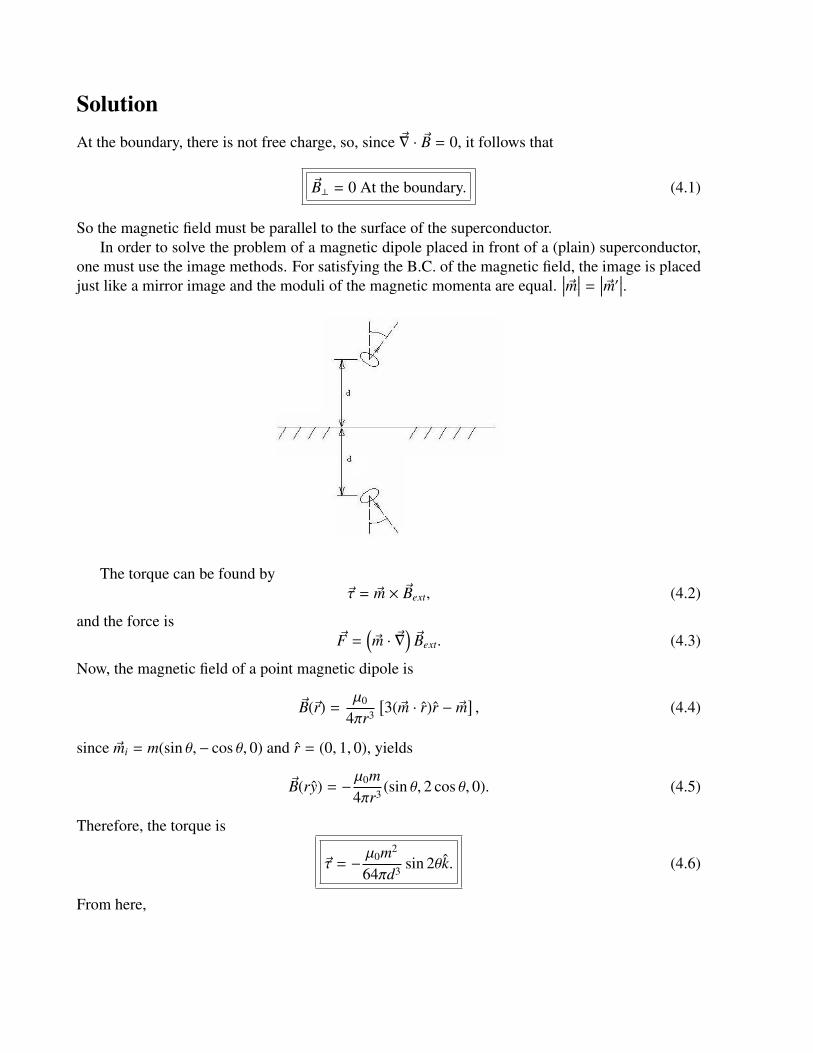
So the magnetic field must be parallel to the surface of the superconductor.In order to solve the problem of a magnetic dipole placed in front of a (plain) superconductor,

one must use the image methods. For satisfying the B.C. of the magnetic field, the image is placedjust like a mirror image and the moduli of the magnetic momenta are equal.

∣∣∣~m∣∣∣ = ∣∣∣~m′∣∣∣.

The torque can be found by~τ = ~m × ~Bext, (4.2)

and the force is~F =

(~m · ~∇

)~Bext. (4.3)

Now, the magnetic field of a point magnetic dipole is

~B(~r) =µ0

4πr3

[3(~m · r)r − ~m

], (4.4)

since ~mi = m(sin θ,− cos θ, 0) and r = (0, 1, 0), yields

~B(ry) = −µ0m4πr3 (sin θ, 2 cos θ, 0). (4.5)

Therefore, the torque is

~τ = −µ0m2

64πd3 sin 2θk. (4.6)

From here,

θ equilibrium0 unstableπ/2 stableπ unstable

3π/2 stable

On the other hand, the force among this two point magnetic dipoles vanish,

~F = 0. (4.7)

4.2 Problem Pr. 4.2the figure shows an uniform magnetic field ~B confined to a cylinder of radius r. The magneticfield decreace in magnitud to a constant rate of 100 gauss/s. What is the instantaneous accelerationexperimented by an electron placed on P1, P2 and P3?. Assume a = 5cm.

SolutionObviously one solves the problem with the help of

~∇ × ~E = −∂~B∂t, (4.8)

or what’s the same, ∮~E · d~l = A

dBdt. (4.9)

The set up has a symmetry and the symmetry left a fixed point (in this case is not just a pointbut a line... the axis of the cylinder), so one takes as path circumference centered at the origin, thus,

the enclosed area is

A(p1) = A(p3) = πa2 (4.10)A(p2) = 0. (4.11)

Axial symmetry assures that∣∣∣∣~E∣∣∣∣ is constant along the chosen path, so

E =A

2πrdBdt. (4.12)

Hence, Ep2 = 0 and

Ep1,p3 =πr2

2πrdBdt=

r2

dBdt, (4.13)

in the −θ direction.Thus,

~a =er

2me

dBdtθ. (4.14)

Now, since 100 Gaußare 10−2T , me = 9.1 ∗ 10−31Kg, e = 1.6 ∗ 10−19C, then

~a ' 5 ∗ 107m/s2. (4.15)

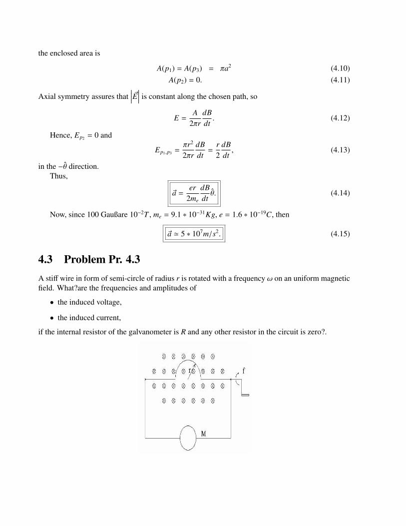
4.3 Problem Pr. 4.3A stiff wire in form of semi-circle of radius r is rotated with a frequency ω on an uniform magneticfield. What?are the frequencies and amplitudes of

• the induced voltage,

• the induced current,

if the internal resistor of the galvanometer is R and any other resistor in the circuit is zero?.

SolutionSince

Φ(t) = BA(t) = BA0 cos(ωt). (4.16)

It follows that

ε = −∂Φ

∂t= ωBA0 sin(ωt). (4.17)

This implies that

Amp(V) = ωBA0, (4.18)

andf req(V) = ω. (4.19)

By Ohm’s law, V = IR, one get

I =ωBA0

Rsin(ωt). (4.20)

∴Amp(I)=

ωBA0

R,

f req(I)= ω.(4.21)

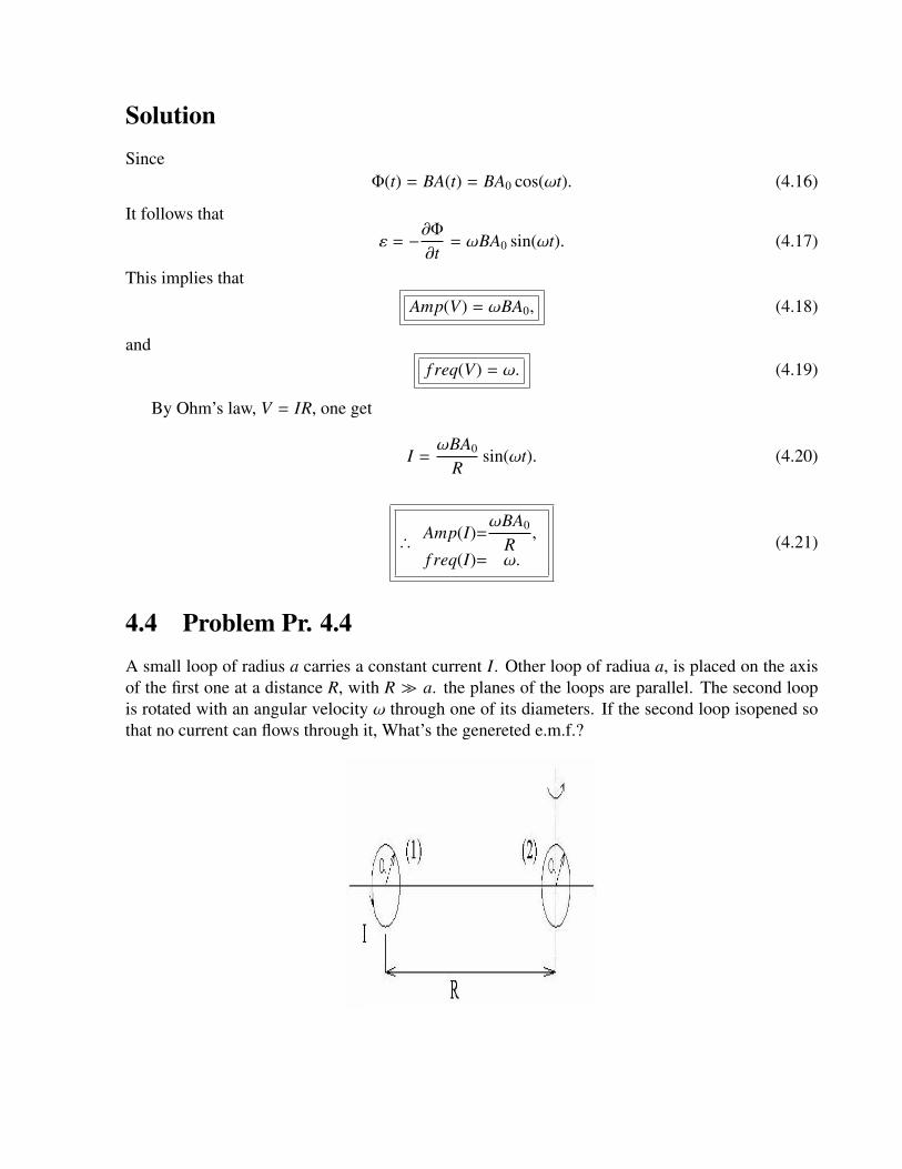
4.4 Problem Pr. 4.4A small loop of radius a carries a constant current I. Other loop of radiua a, is placed on the axisof the first one at a distance R, with R a. the planes of the loops are parallel. The second loopis rotated with an angular velocity ω through one of its diameters. If the second loop isopened sothat no current can flows through it, What’s the genereted e.m.f.?

Solution

The second loop is spinning into the magnetic field generated by the first one, so the induced e.m.f.is

ε = −dΦdt= −B

dAdt, (4.22)

where A is understands like a given area whose boundary is the loop.Nonetheless, as the second loop has been cutted, the induced current cannot be generated and

the end-points behave like a capacitor, which produce a potential in the inverse direction of ε, so,the total e.m.f. vanish,

ε = 0. (4.23)

Other way of seeing the above result is that once one has cutted the loop there isn’t a close path,so the definition of e.m.f. loose its sense.

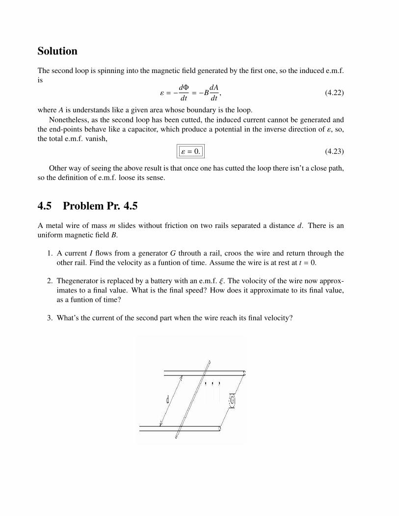
4.5 Problem Pr. 4.5

A metal wire of mass m slides without friction on two rails separated a distance d. There is anuniform magnetic field B.

1. A current I flows from a generator G throuth a rail, croos the wire and return through theother rail. Find the velocity as a funtion of time. Assume the wire is at rest at t = 0.

2. Thegenerator is replaced by a battery with an e.m.f. ξ. The volocity of the wire now approx-imates to a final value. What is the final speed? How does it approximate to its final value,as a funtion of time?

3. What’s the current of the second part when the wire reach its final velocity?

SolutionIn the first case,since the current is constant, one can write the Lorentz force as

~F = m~a = l~I × ~B, (4.24)

or what’s equal, so that ~I⊥~B,

a =lIBm= const., (4.25)

so,

v =lIBm

t. (4.26)

In the second case, the generator is changed by a battery whose e.m.f. is ε, by Ohm’s law,

I =(ε − εind)

R. Faraday’s yields

εind = − −∂Φ

∂t= −Blv, (4.27)

therefore,

dvdt=

lIBm

=lBmR

(ε − lBv) . (4.28)

One can solve this equation by separation of variables, then

v(t) =ε

lB−

AlB

e−l2B2mR t. (4.29)

Finally, the initial condition v(t = 0) = 0, yields

v(t) =ε

lB

(1 − e−

l2B2mR t

). (4.30)

The asymptotic limit of the velocity is v =ε

lB, and again by Ohm’s law,

I = 0. (4.31)

4.6 Problem Pr. 4.6A toroidal solenoid of N turns has a square transversal section. Each side of the square has lengtha and the inner radius is b.

1. Show that the self-inductance is

L =N2a

2πε0c2 ln(1 +

ab

).

2. Express in similar terms the mutual inductance of a system formed by the solenoid and astraight wire placed on the axis of symmetry of the solenoid.

3. Find the rate of the self- and mutual inductances.

Solution

Since ,

W =12

LI2 =1

2µ0

∫B2d3r, (4.32)

and for the torus magnetic field,

Bx =NI

2πε0c2

1b + x

. (4.33)

In cylindric coordinates,

12µ0

∫B2d3r =

12µ0

∫ a+b

bdr r

∫ 2π

0dθ

∫ a

0dz

µ20N2I2

4π2

1r2

=N2I2a4πε0c2

∫ a+b

b

drr

=N2I2a4πε0c2 ln

(1 +

ab

). (4.34)

Therefore,

L =N2a

2πε0c2 ln(1 +

ab

). (4.35)

Similarly,

MI1I2 =1µ0

∫~B1 · ~B2d3r, (4.36)

and so that B1 , 0 just inside T 2,it follows that

B1 =µ0NI1

2πrθ and B2 =

µ0I2

2πrθ, (4.37)

then,

M =Na

2πε0c2 ln(1 +

ab

). (4.38)

Finally,

LM= N. (4.39)

4.7 Problem Pr. 4.7A pair of plane loops, each one of area A and carring a current I, are separated a distance r.

The normals of the loops form angles α1 and α2 respect to the line which joints the loops andthese angles live on the same plane.

1. Find the mutual inductance. Assume that radii are much more smaller than the separation.

2. Using the expression for M, find the magnitud and direction of the force among the loops.

3. How would be the force if one reverse the current in one or both loops?

SolutionThemagnetic field of a magnetic dipole is

~B(~r) =µ0

4πr3

[3(~m · r)r − ~m

]. (4.40)

If one choose the origin of coordinates at the place of the first dipole, s.t. the y axis coincide withthe jointing line of the dipoles, then

~m = m(0, cosα1, sinα1), (4.41)

andr = (0, 1, 0). (4.42)

Therefore,~B(R) =

µ0m4πR3

[2 cosα1y − sinα1z

]. (4.43)

Additionally, the vector corresponding to the area of the second dipole is

~A2 = A(0, cosα2, sinα2), (4.44)

thus, the flux of the magnetic field generated by (1) through the surface of (2), is

Φ2 = ~B1(R) · ~A2 =µ0mA4πR3

(2 cosα1 cosα2 − sinα1 sinα2) . (4.45)

Then,

M =µ0A2

4πR3(2 cosα1 cosα2 − sinα1 sinα2) . (4.46)

Furthermore, the force between the to loopsis given by

~F = I2~∇1M, (4.47)

by using the gradient in spherical coordinates, it follows that,

~F = −µ0I2A2

4πR4

[3(2 cosα1 cosα2 − sinα1 sinα2)r + (2 cosα1 sinα2 + sinα2 cosα2)θ

]. (4.48)

Obviously, if one reverse one (or both) current(s), is just like changing the corresponding angleθi → θi + π in the equation (4.48).

4.8 Problem Pr. 4.8A metal rod is magnetized along the azimutal direction. What dependence on the radius can Mhave so that the net magnetic charge in the system vanish?

SolutionSo, one have thet ~M = f (r)θ.

If the material is “uniformly" magnetized, it must satisfy that

~∇ · ~M = ~∇ · ~M = 0. (4.49)

In cylindrical coordinates the only components that contributes are

~∇ · ~M =1r∂θ(r f (r)) = 0, (4.50)

~∇ · ~M =1r∂θ(r f (r)) = 0. (4.51)

Equation (4.50) doesn’t make a constraint on f , but (4.51) impose that

f (r) =1r. (4.52)

4.9 Problem Pr. 4.9A long wire of radius a carries a current I and it’s surrounded coaxially by a long holed ironcylinderwith relative permeability Km. The inner radius of the cylinder is b and the external is c.Calculate the total flux of ~B inside a section of lenght l of the cylinder.

Find the current density on the inner and outer surface of the cylinder, also the directions of thecurrents relative to the current of the wire.

Find the equivalent current density inside the cylinder.Find ~B at r > c from the wire. How’s it affected if the cylinder is taken away?

SolutionThe boundary conditions for the Magnetic field are (without free currents)

H(1)⊥ = H(2)

⊥ , (4.53)B(1)

= B(2) . (4.54)

Since the magnetic fiel d generated by a wire is

~B =µ0I2π

1rθ ⇒ ~Bm =

µI2π

1rθ, (4.55)

then,

Φm =µIl2π

∫ c

b

drr= Km

µ0Il2π

ln(cb

). (4.56)

Also, since ~Js = ~M × n|s, gives the current density on the surface of the conductor. From(4.56)it follows that,

~M =I

2πr(Km − 1)θ, (4.57)

thus, on the inner surface,

~J =I

2πb(Km − 1)z, (4.58)

and in the outer surface,

~J = −I

2πc(Km − 1)z. (4.59)

The internal current is

~J = ~∇ × ~M =1r∂r(rMθ) = 0. (4.60)

Finally, since the currents at r = b and r = c are the same, the magnetic field outside thecylinder is just the sameas without the cylinder,

~B(r > c) =µ0I2πr

θ. (4.61)

Part II

Quantum Mechanics

61

Chapter 5One-dimensional Problems

5.1 Problem 1...A particle of mass m is confined to a 1-dimensional region 0 ≤ x ≤ a by the potential

V(x) =

0 if 0 ≤ x ≤ a∞ otherwise (5.1)

At t = 0, the wave function is

ψ(x, t = 0) =

√85a

(1 + cos

(πxa

))sin

(πxa

). (5.2)

Calculate

a. ψ(x, t0) for t0 > 0.

b. The energy of this wave at t = 0 and t = t0.

c. What’s the probability of finding such a particle in the right half of the well?

SolutionThe Schrödinger equation for a particle in an 1-dimensional box is

∂xψ(x) + ω2ψ(x) = 0, (5.3)

where ω2 =√

2mE~2 . By imposing the boundary conditions ψ(0) = ψ(a) = 0, we get the solution,

ψ(x) = A sin(ωx), (5.4)

63

with

ωa = nπ ⇒ En =n2π2~2

2ma2 with n ∈ N∗. (5.5)

Therefore, (5.2) is nothing but a lineal combination of the solutions with n = 1 and n = 2

ψ(x, 0) =

√8

5asin

(πxa

)+

√25a

sin(2πx

a

). (5.6)

Next, by applying the evolution operator, U(t) = e−ı~Ht, we obtain

ψ(x, t) =

√85a

e−ıπ2~2ma2 t sin

(πxa

)+

√2

5ae−

2ıπ2~ma2 t sin

(2πx

a

). (5.7)

Then, the VEV of the energy is the expectation value of the Hamiltonian,

〈H〉t =∫ a

0dxψ∗(x, t)

(−~2

2m∂2

x

)ψ(x, t)

=4π2~2

5ma3

∫ a

0dx sin2

(πxa

)+

4π2~2

5ma3

∫ a

0dx sin2

(2πx

a

)+ ∼

∫ a

0dx sin

(πxa

)sin

(2πx

a

)=

4π2~2

5ma2 , (5.8)

so that, ∫ π

0dxsin2nx =

π

2. (5.9)

Indeed, since (5.8) is time independent, it follows that

〈E〉0 = 〈E〉t =4π2~2

5ma2 . (5.10)

Finally,P(x, t)dx = |ψ(x, t)|2dx, (5.11)

then,

P(x ≥ a/2, t) =∫ a

a/2dxψ∗(x, t)ψ(x, t)

=8

5a

∫ a

a/2dx sin2

(πxa

)+

25a

∫ a

a/2dx sin2

(2πx

a

)8

5a

∫ a

a/2dx sin

(πxa

)sin

(2πx

a

)cos

(3π2~2t2ma2

)=

12−

1615π

cos(3π2~2t2ma2

), (5.12)

because ∫ a

a/2dx sin2

(nπxa

)=

a4

(5.13)∫ a

a/2dx sin

(πxa

)sin

(2πx

a

)= −

2a3π. (5.14)

Note that (5.12) is granther than 0 for whatever value of t.

5.2 Problem 2...A particle of mass m moves on a 1-dimensional potential

V(x) =λδ

(x − L

2

)if 0 ≤ x ≤ L

∞ otherwise(5.15)

a. Find the transcendental equation for the eigenvalues of the energy (In terms of m, L and λ).

b. Find the pair of lowest energies levels and corresponding eigenstates for Lm/~ = 4 and λ/~ = 2.

SolutionLet’s define, like before,

ω2 =2mE~2 . (5.16)

The solution to the homogeneous (i.e., without the Dirac’s delta distribution), is

ψ(x) = A sin(ωx) + B cos(ωX). (5.17)

We should consider different solutions in both regions, left- and right-side of the delta. So, byimposing the boundary conditions,

ψ(0) = ψ(L) = 0, (5.18)

we get,

ψI(x) = A sin(ωx) (5.19)ψII(x) = B sin(ωx) − tan(ωx) . (5.20)

Then, by continuity ψI(L/2) = ψII(L/2), it follows that

A sin(ωL/2) = B sin(ωL/2) − tan(ωL/2) , (5.21)

that can be rewritten asB = −A cos(ωL), (5.22)

by using the relation

tan(x/2) =1 + cos(x)

sin(x). (5.23)

Finally, we must use the discontinuity condition on the derivative of the wave function due tothe delta distribution,

ψ′II(L/2) − ψ′I(L/2) =2mλ~2 A sin(ωL/2), (5.24)

which gives us the relation,

cos(ωL)[cos

(ωL2

)+ tan(ωL) sin

(ωL2

)]+ cos

(ωL2

)= −

2mλω~2 sin

(ωL2

). (5.25)

This last equation can be reduce, by using the half angle formulae for trigonometric functions, to

tan(ωL2

)= −

ω~2

mλ, (5.26)

or

tan

Lm2~

√2Em

= √2Em~

λ. (5.27)

Considering the values Lm/~ = 4 and λ/~ = 2, we get

tan(x) = −x/4, (5.28)

with

x = 2

√2Em. (5.29)

The lowest eigenvalues for this equation are (x=0 is not allowed because of the uncertaintyrelations) x = 2.6 and x = 5.3, or in term of energy, E0 .85m and E1 3.5m.

5.3 Problem 3...

A simple model for the states of an electron in a 1-dimensional system is

H =N∑

n=1

E0|n >< n| +N∑

n=1

W |n >< n + 1| + |n + 1 >< n| , (5.30)

where |n >n=1...N is an orthonormal basis and periodic conditions |N + j >= | j > are assumed. E0

and W are given parameters.Calculate the eigenstates and eigenenergies.

Part III

Thermodynamics and Statistical Mechanics

69

Chapter 6Probability

6.1 Problem. Reif 1.1

SolutionIn order to get less than 6 point with a set of 3 dice, one should get

Throw # of permutations1,1,1 11,1,2 31,1,3 31,1,4 31,2,3 61,2,2 32,2,2 1

Then,

Pr =Nr

N=

2063 = 9.26 ∗ 10−2. (6.1)


Solution1.

P =6!

5!1!

(16

) (56

)5

= 0.402 (6.2)

2.

P = 1 −(56

)6

= 0.667 (6.3)

71

3.

P =6!

4!2!

(16

)2 (56

)4

= 0.2 (6.4)


SolutionEach digit, has 5 possible choices for been < 5 and 5 of been ≥ 5, then, p = q = 1

2 .Thus,

P =10!5!5!

(12

)10

= 0.246. (6.5)


Solution1.

P(N/2) =N!

N2 ! N

2 !

(12

)N

. (6.6)

2. If N is odd, either n1 or n2 is odd and the other is even, so

P(m = 0) = 0. (6.7)


Solution1.

P =(56

)N

. (6.8)

2.

P =(56

)N−1 16. (6.9)

3.# pull =

1Pshoot

= 6. (6.10)


Solution

It is known that ma = (2n − N)a, then

m = 2n − N (6.11)m2 = 4n2 − 4Nn + N2 (6.12)m3 = 8n3 − 12Nn2 + 6N2n − N3 (6.13)m4 = 16n4 − 32Nn3 + 24N2n2 − 8N3n + N4. (6.14)

Next,

na =

(p∂

∂p

)a

(p + q)N , (6.15)

then1, (p∂

∂p

)(p + q)N = N p(p + q)N−1 (6.16)(

p∂

∂p

)2

(p + q)N = N p[(p + q)N−1 + (N − 1)p(p + q)N−2

](6.17)(

p∂

∂p

)3

(p + q)N = N p[(p + q)N−1 + 3(N − 1)p(p + q)N−2

+(N − 1)(N − 2)p2(p + q)N−3]

(6.18)(p∂

∂p

)4

(p + q)N = N p[(p + q)N−1 + 7(N − 1)p(p + q)N−2

+6(N − 1)(N − 2)p2(p + q)N−3

+(N − 1)(N − 2)(N − 3)p3(p + q)N−4]

(6.19)

Using that p + q = 1, and substituting (6.16)-(6.19) into (6.11)-(6.14), one gets

m = 0 (6.20)m2 = N (6.21)m3 = 0 (6.22)m4 = 2N4 + 2N3 − 3N2 + 4N (6.23)

1You must check it by yourself because it does not coinside neither with the Reif results nor the resultofa friend ofmine.


Solution

W ′(n) =2∑

i1=1

· · ·

2∑iN=1

ωi1 · · ·ωiN

=

2∑i1=1

ωi1 · · ·

2∑iN=1

ωiN

= (ω1 + ω2) · · · (ω1 + ω2)= (ω1 + ω2)N . (6.24)

From the binomial theorem, it follows that the restriction of ω1 to occurs n times is

W(n) =N!

n!(N − n)!ωn

1ωN−n2 . (6.25)

Chapter 7Thermodynamics

7.1 Problem. Huang 1-1

SolutionFor an adiabatic process, ∆Q = 0, so, the first law becomes

dU = dW = −PdV. (7.1)

From the kinetictheory of ideal gases, the internal energy is

U =32

NkT, (7.2)

then,

dU =32

NkdT. (7.3)

Hence,32

NkdT = −PdV = −NkT

VdV, (7.4)

where the ideal gas equation of states has been used. Integrating (7.4), the result

32

∫ T

T0

dTT= −

∫ V

V0

dVV

V0

V=

(TT0

)3/2

. (7.5)

Since,

Vi =NkTi

Pi, (7.6)

75

it is possible to change V by T , therefore,

PP0=

(TT0

)5/2

, (7.7)

and also, in the same way,PP0=

(V0

V

)5/3

. (7.8)

Chapter 8Statistical Mechanics

8.1 Problem G.-C. 2.2

SolutionSince

Ω = Ω1Ω2, (8.1)

it follows that

Ω2d f (Ω)

dΩ=

dΩ1

dΩ1, (8.2)

Ω1d f (Ω)

dΩ=

dΩ2

dΩ2. (8.3)

The chain rule gives,d

d lnΩf =

dΩd lnΩ

d fdΩ

, (8.4)

thus, (8.2) times Ω1 gives,

Ωd f (Ω)

dΩ= Ω1

d f (Ω1)dΩ1

⇒d f (Ω)d lnΩ

=d f (Ω1)d lnΩ1

, (8.5)

and similarly,d f (Ω)d lnΩ

=d f (Ω2)d lnΩ2

. (8.6)

Furthermore, the Ω2 derivative of (8.5) and Ω1 derivative of (8.6) vanish, so

ddΩ2

d f (Ω)d lnΩ

= 0 (8.7)

ddΩ2

d f (Ω)d lnΩ

= 0, (8.8)

77

then,f (Ω) = k lnΩ + Ω0, (8.9)

with k a constant.By the initial condition,

f (Ω1) + f (Ω2) = f (Ω),

if the integration constant Ω0 is not zero, it adds. So, the integration constant must be zero.

8.2 Problem G.-C. 2.5The energy levels allow for a bi-dimensional harmonic oscillator are εi = (n + 1)hν and theirdegenerancy is ωi = (n + 1). Show that the partition function for those oscillators is the square ofthe partition function for the one dimensional oscillator.

SolutionThe available data is εi = (n + 1)hν and ωi = n + 1. From the definition,

Z2 =

∞∑n=0

(n + 1)e−(n+1)hνβ

= −∂

∂(hνβ)

∞∑n=0

e−(n+1)hνβ

= −∂

∂(hνβ)e−hνβ

1 − e−hνβ

= −∂

∂(hνβ)1

ehνβ − 1

=ehνβ

(ehνβ − 1)2 . (8.10)

Since the partition function for the one-dimensional harmonic oscillator is

Z1 =e

12 hνβ

(ehνβ − 1), (8.11)

one conclude that

Z2 = (Z1)2. (8.12)

8.3 Problem G.-C. 2.6Obtain the eq. (2.29) of the book.

SolutionFrom

U =32

Nhν + 3Nhν

e−hνkT − 1

, (8.13)

it follows that,

Cv =

(∂U∂T

)v

= 3Nhν∂

∂T1

e−hνkT − 1

= 3Nh2ν2

kT 2

ehvkT(

ehvkT − 1

)2

= 3Nk(

hνkT

)2 ehvkT(

ehvkT − 1

)2 . (8.14)

Finally,

Cv = 3Nk(

hνkT

)2 ehvkT(

ehvkT − 1

)2 (8.15)

8.4 Problem G.-C. 2.8Repit the calculus of 〈µz〉 when J = 1

2 . Compare the results with the eqs. (2.37)–(2.39) in thetextbook.

SolutionOne have that

Z 12=

1/2∑m=−1/2

egµ0Hmβ, (8.16)

and

〈µz〉 =

1/2∑m=−1/2

egµ0Hmβ =∂

∂Hβln

1/2∑m=−1/2

egµ0Hmβ. (8.17)

Now,1/2∑

m=−1/2

egµ0Hmβ = 2 coshgµ0Hβ

2, (8.18)

then,∂

∂Hβln 2 cosh

(gµ0Hβ2

)=

12

gµ0 tanh(gµ0Hβ

2

), (8.19)

thus,

〈µz〉 =12

gµ0 tanh(gµ0Hβ

2

). (8.20)

On the other hand,

〈µz〉 = gµ0JBJ(η), (8.21)

with η = gµ0Hβ and

BJ(η) =1J

[(J + 1/2) coth

(J +

12

)η −

12

cothη

2

]. (8.22)

For J = 1/2, it follows that

B1/2(η) = 2[coth η −

12

cothη

2

]. (8.23)

By using the identity,

tanh 2x =2 tanh x

1 + tanh2 x, (8.24)

the last equation can be written as,

B1/2(η) = 2[1 + tanh2 η/2

2 tanh η/2−

12

cothη

2

]= tanh η/2, (8.25)

and finally,

〈µz〉 =12

gµ0 tanh(gµ0Hβ

2

). (8.26)


Show that a solid obeying Einstein model has

S = −3Nk∂

∂T

[T ln

(1 − e−

hνkT)]. (8.27)

Discuss physically the limits of low and high frequencies. What rôle plays the zero point energy?

SolutionSince,

Z0 =

∞∑n=0

e−(n+1/2)hνβ =e−

12 hνβ

1 − e−hνβ , (8.28)

it follows thatF = −NkT ln Z0 =

32

Nhν + 3NkT ln(1 − e−hνβ

). (8.29)

Finally from the Maxwell relation,one get

S = −(∂F∂T

)V= −3Nk

∂

∂T

[T ln

(1 − e−

hνkT)]. (8.30)

8.6 Problem G.-C. 3.1Deduce the eq. (3.5) of the text.

SolutionSince

U = N∑∞

i=0 εie−εiβ∑∞j=0 e−ε jβ

= −N∑∞

j=0 e−ε jβ

∂

∂β

∞∑i=0

e−εiβ

= −N∂

∂βln

∞∑i=0

e−εiβ

,(8.31)

Now, by calling

Z0 =

∞∑i=0

e−εiβ, (8.32)

and since the chain rule gives

∂

∂β=∂T∂β

∂

∂T⇒

∂

∂β= −kT 2 ∂

∂T, (8.33)

finally one get,

〈E〉 = NkT 2 ∂

∂Tln Z0. (8.34)


Obtain the eq. (3.8) of the text, from the definition of entropy.

Solution

By the definition of the entropy,

S = −(∂F∂T

)V. (8.35)

Since

F = −NkT

ln V +32

ln T + ln(2πmk

h2

)3/2 , (8.36)

then,

S = Nk

ln V +

32

ln T + ln(2πmk

h2

)3/2 + 3

2

. (8.37)

By substituting R = Nak and s = S/n,

sR= ln V +

32

ln T +32+ ln

(2πmk

h2

)3/2 . (8.38)


Use the eqs. (3.17)-(3.20) of the textbook, to obtain the eqs. (3.21) and (3.22) therein.

Solution

Beginning from the corrected distribution

Wn1,n2 =∏

i, j

1

n(1)i !n(2)

j !, (8.39)

the numberof states is given by

Ω =

′∑n(1),n(2)

∏i, j

1

n(1)i !n(2)

j !, (8.40)

with the constrints ∑i

n(1)i = N1, (8.41)∑

i

n(2)i = N2, (8.42)∑

i

n(1)i ε(1)

i +∑

j

n(2)j ε

(2)j = E. (8.43)

Calling

t(n(1), n(2)) =′∑

n(1),n(2)

∏i, j

1

n(1)i !n(2)

j !, (8.44)

and using

δt(n(1), n(2)) =∑

i

∂t

∂n(1)i

δn(1)i +

∑j

∂t

∂n(2)j

δn(2)j , (8.45)

and additionally, ∑i

δn(1)i = δN1 = 0, (8.46)∑

i

δn(2)i = δN2, (8.47)∑

i

δn(1)i ε(1)

i +∑

j

δn(2)j ε

(2)j = δE = 0. (8.48)

Thus,

δt(n(1), n(2)) =∑

i

∂t

∂n(1)i

+ α1 + β1ε(1)i

δn(1)i

+∑

j

∂t

∂n(2)j

+ α2 + β2ε(2)j

δn(2)j , (8.49)

with α’s and β’s Lagrange multipliers.Now,

ln t(n(1), n(2)) = −∑

i

ln(n(1)i !) −

∑j

ln(n(2)j !)

= −∑

i

n(1)i ln(n(1)

i ) + N1 −∑

j

n(2)j ln(n(2)

j ) + N2, (8.50)

since,∂

∂n(α)a

ln t(n(1), n(2)) = − ln n(α)a − 1, (8.51)

then, as each term of the sum on (8.49) must vanish independently, it follows that

ln n(α)a = α(α) + β(α)ε

α)a ⇒ n(α)∗

a = eα(α)eβ(α)εα)a . (8.52)

Finally, from the restrictions, ∑a

n(α)∗a =

∑a

eα(α)eβ(α)εα)a = N(α), (8.53)

one gets

eα(α) =N(α)∑

a eβ(α)εα)a, (8.54)

by definition,Z(α) =

∑a

eβ(α)εα)a , (8.55)

thus,

n(1)∗i =

N1

Z1eβ1ε

(1)i , (8.56)

and

n(2)∗j =

N2

Z2eβ2ε

(2)j . (8.57)

8.9 Problem G.-C. 3.4Use the result of the previous problem to deduce the eqs. (3.23a) and (3.23b) in the text.

Solution

S = k ln t(n(1), n(2))max

= −k∑

i

n(1)∗i ln(n(1)∗

i ) + kN1 − k∑

j

n(2)∗j ln(n(2)∗

j ) + kN2

= −k∑

i

n(1)∗i ln(n(1)∗

i ) + kN1 − k∑

j

n(2)∗j ln(n(2)∗

j ) + kN2

= −kβE − kN1(ln N1 − 1 − ln Z1) − kN2(ln N2 − 1 − ln Z2)

= k lnZN1

1

N1!+ k ln

ZN22

N2!+ −

ET. (8.58)

Thus,

F = −kT lnZN1

1

N1!ZN2

2

N2!

. (8.59)

8.10 Problem G.-C. 3.5The energy of the one-dimensional harmonic oscillator is

ε(x, p) =p2

2m+

12

mω2x2. (8.60)

Calculate the clasical partition function and the termal propertiesof a system of 3N lineal oscil-lators. Compare these results with the one of the second chapter of the textbook.

SolutionTwo different approaches for solving this problem will be given, the first is by using the definitionof the classical partition function and the second by the micro-canonical partition function.

Classical Partition FunctionBy definition, the classical partition function for a single harmonic oscillator is

Z =1~

∫R

dx∫R

dpe−(

p22m+

12 mω2 x2

)β, (8.61)

since, ∫R

dx e−ax2=

√π

a, (8.62)

it follows that (8.61) yields,

Z =kT~ω

. (8.63)

Therefore,

F = −kT ln Z = −kT lnkT~ω

, (8.64)

so, using Maxwell’srelations, one get

P = −

(∂F∂V

)T= 0, (8.65)

S = −

(∂F∂T

)V= k

[1 + ln

(kT~ω

)], (8.66)

U = F + TS = kT, (8.67)

thus,

S (E,V) = k[1 + ln

( E~ω

)]. (8.68)

Repiting the above precess for 3N harmonic oscillators,

Z =(

kT~ω

)N

, (8.69)

where the N! coming from the Gibbs factor is not consider. Hence,

F = −3NkT ln(

kT~ω

), (8.70)

P = 0, (8.71)

S = 3Nk[1 + ln

(kT~ω

)], (8.72)

U = 3NkT, (8.73)

thus,

S (E,V,N) = 3Nk[1 + ln

( E3N~ω

)]. (8.74)

Micro-canonical Partition Function

8.11 Problem G.-C. 3.15

SolutionA relativistic ideal gas is composed by relativistic free particles, so its Hamiltonian is given by

H =N∑

i=1

mc2

1 + (

~pmc

)21/2

− 1

, (8.75)

then, for a single particle its partition function is

Z(T,V, 1) =1h3

∫d3q

∫d3 pe

−βmc2[

1+(~p

mc

)2]1/2−1

=Vh3 eβmc2

∫d3 pe

−βmc2[

1+(~p

mc

)2]1/2

=4πVh3 eβmc2

∫ ∞

0dpp2e

−βmc2[

1+( pmc )

2]1/2

. (8.76)

In order to perform the integral one can substitute pmc = sinh x, therefore,

Z(T,V, 1) =4πVh3 (mc)3eβmc2

∫ ∞

0dx cosh x sinh2 xe−βmc2 cosh x, (8.77)

calling u = βmc2,

Z(T,V, 1) =4πVh3 (mc)3eu

∫ ∞

0dx cosh x sinh2 xe−u cosh x. (8.78)

Using the identity sinh x cosh x = 12 sinh 2x,

Z(T,V, 1) = 4πV(mc

h

)3 12

eu∫ ∞

0dx sinh 2x sinh xe−u cosh x. (8.79)

The above integral is solved by∫ ∞

0dx sinh x sinh γxe−u cosh x =

γ

uK2(u). (8.80)

The nonrelativistic limit is u = βmc2 → ∞, i.e., mc2 >> kT . Using that

K2(z) √π

2ze−z,

as long as z→ ∞, so

Z(T,V, 1)→ 4πV(mc

h

)3(

1βmc2

)3/2 √π

2= V

(2πmkT

h2

)3/2

, (8.81)

which agrees with the ideal gas.The high temperature limit is kT >> mc2, for which K2(u) 2

u , and so

Z(T,V, 1)→ 8πV(kThc

)3

, (8.82)

this last is the partition function of an ultra-relativistic ideal gas.Finally, the partition function of the ideal gas of N particles is

Zn =1

N!(Z1)N =

1N!

[4πV

(mch

)3eβmc2 K2(βmc2)

βmc2

]N

. (8.83)

From this,

F = −kT ln ZN

= −NkT − Nmc2 − NkT ln[4πV

(mch

)3eβmc2 K2(βmc2)

βmc2

], (8.84)

and

P = −(∂F∂V

)=

NkTV

, (8.85)

µ =∂F∂N= −kT ln

[4πV

(mch

)3eβmc2 K2(βmc2)

βmc2

]− kT − mc2, (8.86)


SolutionConsider the Maxwell-Boltzmann distribution,

f (~v)d3v =( m2πkT

)3/2e−

m2kT ~v

2d3v. (8.87)

Since, ∫ ∞

0e−ax2

dx =√π

a, (8.88)

the total contribution to vx is the integral over y and z,

f (vx)dv =( m2πkT

)1/2e−

m2kT v2

xdvx. (8.89)

Then, the probability of finding a particle with celerity on x between 0 and vx0 , is

Pr(0 ≤ vx ≤ vx0) =( m2πkT

)1/2 ∫ vx0

0e−

m2kT v2

xdvx, (8.90)

by defining vm =

√2kTm and x = vx

vm, one get

n = NPr(0 ≤ vx ≤ vx0)

= N( m2πkT

)1/2 ∫ vx0

0e−

m2kT v2

xdvx

= N1√π

∫ x0

0dxe−x2

=N2

er f (x0). (8.91)

Thus,

n =N2

er f (x0). (8.92)



f (~v)d3v =( m2πkT

)3/2e−

m2kT ~v

2d3v. (8.93)

This time the interest turns to the total celerity, so one can write the Maxwell-Boltzmann dis-tribution in spherical coordinates, where d3v = dvv2dΩ, and so

Pr(0 ≤ v ≤ v0) = 4π( m2πkT

)3/2 ∫ v0

0dvv2e−

m2kT v2

. (8.94)

by defining vm =

√2kTm and x = vx

vm, one get

Pr(0 ≤ v ≤ v0) =4√π

∫ x0

0dxx2e−ax2

∣∣∣∣∣∣a=1

=4√π

(−∂

∂a

) ∫ x0

0dxe−ax2

∣∣∣∣∣∣a=1

= −2∂

∂a1√

aer f (

√ax0)

∣∣∣∣∣∣a=1

= er f (x0) −2√π

x0e−x20 . (8.95)

Thus,

n = N[er f (x0) −

2√π

x0e−x20

]. (8.96)

8.14 Problem G.-C. 4.5The traslacional energy of a molecul is ε = 1

2mv2. Write the Maxwell distribution function in termsof ε


f (~v)d3v =( m2πkT

)3/2e−

m2kT ~v

2d3v. (8.97)

In terms of celerity,

f (v)dv = 4π( m2πkT

)3/2e−

m2kT v2

v2dv. (8.98)

By changing

ε =mv2

2, v =

√2εm, vdv =

dεm, (8.99)

then,

f (ε)dε = 2πN(πkT )−3/2√εe−ε

kT dε. (8.100)

8.15 Problem G.-C. 4.8For a gas in equilibrium, calculate

⟨~v⟩,⟨v2

x

⟩,⟨v3

x

⟩and

⟨(vx + bvy)2

⟩, where b is a constant.

SolutionSince the set up is confined to a volume V , it’s invariant under parity symmetry, so the mean valueof the velocity vanish, ⟨

~v⟩= 0. (8.101)

On the other hand, the average energy by d.o.f. is 12kT . Hence, E = 1

2mv2, it follows that,

⟨v2

x

⟩=

Nm

kT. (8.102)

By the same symmetry argument as the first case, one get

⟨v3

x

⟩= 0, (8.103)

as well as the higher odd momenta.Also, ⟨

(vx + bvy)2⟩=

⟨v2

x

⟩+ 2b

⟨vxvy

⟩+ b2

⟨v2

y

⟩=

(1 + b2

) NkTm

. (8.104)

Physically, the higher distribution momenta are irrelevant, because there are not fundamentalquantities related with those.


SolutionThe canonical partition function for an ideal gas is

Z1 = V(2πmkT

h2

)3/2

, (8.105)

andZn =

1N!

ZN1 . (8.106)

Sinceeβµ

∑i

gie−βεi = N, (8.107)

then

A =N∑

i gie−βεi=

NZN, (8.108)

so, by taking logarithm and β =1

kT,

µ

kT= ln

(NV

)+

32

ln(

h2

2πmkT

). (8.109)


Solution

The degeneration parameter is

ξ =VN

(2πmkT

h2

)3/2

, (8.110)

so for an isometric process,

T ≤VN

h2

2πmk. (8.111)

Moreover, taking

V = 1cm3 (8.112)N = 1mol (8.113)k = 1.38 ∗ 10−16erg.K−1 (8.114)h = 6.626 ∗ 10−27erg.s, (8.115)

one gets,

Element Molecular Mass Tc(K)H2 2 108.6D2 4 54.33He 4 54.33Ar 40 5.44Cl2 70 3.07


SolutionFor Helium, Tc = 54.33K, so T = 300K Tc, which implies ξ 1. In what follows the quantitesT = 300K, V = 1cm3 and N = 1mol will be used.

Γ(ε) =18

4π3

(8mεa2

h2

)3/2

=πV6

(8mεh2

)3/2

. (8.116)

The number of levels

〈Γ(ε)〉 =πV6

(8mh2

)3/2 ⟨ε3/2

⟩. (8.117)

Now, ⟨ε3/2

⟩=

NZ

∫ ∞

0ρ(ε)ε3/2e−βεdε

= 2πN(

12πkT

)3/2 ∫ ∞

0dε ε2e−βε

= 4πN(kT2π

)3/2

, (8.118)

then

〈Γ(ε)〉 = N8V

3π

(2πmkT

h2

)3/2 . (8.119)

Finally sincemNa= 4gr/mol,

〈Γ(ε)〉N= 6.63 ∗ 1024. (8.120)

And

N =PVkT= 2.4 ∗ 103, (8.121)

Helium molecules.


SolutionSince gi indicates the number of cells, and ni the number of particles, if gi >> ni,paticles can be dis-tribute without a ‘strong’ interaction among them. So they do not note the quantum characteristicsof symmetric or anti-symmetric wave function.


SolutionAs in section 8.18,

ξ =VN

(2πmkT

h2

)3/2

. (8.122)

Since ρ = 107gr/mol, T = 107K andmHe

Na= 4gr/mol, a direct computation gives

ξ = 32. (8.123)


SolutionSince the partition function is

Z =∑

i

gie−βεi , (8.124)

in order to past to the classical the differences between energies must satisfy the condition

∆ε

εi∼ 0. (8.125)

In doing this, the energies change to

εi −→ ε(~r, ~p) =~p2

2m+ ϕ(~r), (8.126)

and similarly the sum turns into an integral,∑i

gi −→1h3

∫dΓ. (8.127)

So, the classical partition function is

Z =1h3

∫dΓe−βε(~r,~p), (8.128)

and finally, the fraction of molecules having momentum between[~p, ~p + d~p

]and position

[~x, ~x + d~x

]is given by

n(~r, ~p)dΓ =Ne−β

(~p22m+ϕ(~r)

)dΓ∫

e−β(~p22m+ϕ(~r)

)dΓ. (8.129)

It’s nothing but the Maxwell-Boltzmann distribution.


SolutionFor a grand canonical ensemble,

P j(N) =1Ξ

e−βE j+αN , (8.130)

so,

〈E〉 =∞∑N0

∑j

E jP j(N)

=1Ξ

∞∑N=0

∑j

E je−βE j+αN

= −∂

∂βlnΞ, (8.131)

then

〈E〉 = −∂

∂βlnΞ. (8.132)

Also,

〈N〉 =∞∑N0

∑j

NP j(N)

=1Ξ

∞∑N=0

NeαN∑

j

e−βE j

= −∂

∂αlnΞ, (8.133)

then

〈N〉 = −∂

∂αlnΞ. (8.134)

Finally, one can useTS = U + Nµ + PV, (8.135)

andPV = kT lnΞ = −EN j + µN − kT ln P j(N). (8.136)

Substituting both result above, yields

TS =

∞∑N=0

∑j

(EN j − µN)P j(N)

− EN j + µN − kT ln P j(N). (8.137)

After average the last expresion, and dividing by T ,

S = −k∞∑

N=0

∑j

P j(N) ln P j(N). (8.138)

8.23 Problem G.-C. 9.13

SolutionSince

F = −kT lnΞ, (8.139)

and by Maxwell relations,

S = −(∂F∂T

)V,µ, (8.140)

it follows that

S = k lnΞkT(∂

∂TlnΞ

)V,µ. (8.141)

For an open system,

Ξ =

∞∑N=0

zNZN , (8.142)

so,

〈E〉 =1Ξ

∞∑N=0

∑j

E je−βE j+αN = −∂

∂βlnΞ. (8.143)

〈E〉 == −∂

∂βlnΞ. (8.144)

8.24 Problem G.-C. 9.14

SolutionSince

F = −kT ln Z, (8.145)

and by Maxwell relations,

P = −(∂F∂V

)T,N

, (8.146)

it follows that

P = kT(∂

∂Vln Z

)T,N

. (8.147)

8.25 Problem H.6.1Show that the three definitions of entropy given by

S = k lnΓ(E) (8.148)= k lnΣ(E) (8.149)= k lnω(E), (8.150)

are equivalent. In the above definitions,

Σ(E) =∫

H≤Ed3N pd3Nq, (8.151)

Γ(E) =∫

E≥H≤E+∆d3N pd3Nq = Σ(E + ∆) − Σ(E), (8.152)

ω(E) =∂

∂EΣ(E). (8.153)

SolutionOne can start from the definition

Σ(E) =∫

H≤Ed3N pd3Nq, (8.154)

which can be written asΣ(E) =

∫ ∞

0Θ(E − H)d3N pd3Nq. (8.155)

Now, for Hamiltonians with only second order dependency on p and q, after certain change of vari-able, the remain integral is nothing but the integral of the posible states bounded by a “hyper"-halfof a 3N-dimensional sphere of radius

√E∗, which is the considered energy, E, scaledby factorscom-

ing from the change of variables.For example, for a single free particle,

E∗ =8mV2/3

h2 E. (8.156)

Since the volume of a 3N-dimensional sphere is

Σ(E) =∫

H≤Ed3N pd3Nq, (8.157)

nonetheless, the interesting part for the problem is

123N Σ(E) =

123N

∫H≤E

d3N pd3Nq, (8.158)

because of the boundaries of the set up. Then, formally

Σ(E) ∼1

23N

E3N/2(3N2

)!. (8.159)

Now,

ω(E) =∂Σ

∂E∆ ∼

3N2∆

EΣ(E), (8.160)

thus,

lnω(E) ∼ lnΣ(E) + ln3N2+ ln

DeltaE

, (8.161)

but

limN→∞

ln NN= 0

δ

E<< E ⇒ ln

∆

E= o(0), (8.162)

so,lnω(E) ∼ lnΣ(E). (8.163)

Also, by (8.162) it follows that

lnΓ(E) = lnω(E) + ln∆ ∼ lnω(E) ∼ lnΣ(E). (8.164)

Finally,

lnΓ(E) ∼ lnω(E) ∼ lnΣ(E). (8.165)

8.26 Problem H.6.2Let the “uniform" ensemble of energy E be defined as the ensemble of all systems of the given typewith energy less than E. The equivalence between the definitions of entropy on the above problemmeans that we should obtain the same thermodynamic functions from the “uniform" ensemble ofenergy E as fro the microcanonical ensemble of energy E. In particular, the internal energy is E inboth ensembles. Explain why this seeminly paradoxical result is true.

SolutionAfter proving the equivalency of the three diferent definitions of the entropy, it follows that in factthe “uniform" ensamble is equivalent to the micro-canonical ensamble. The reason underlying this

situation is that the rate at which the number of states grows with energy is so abrupt that the maincontribution is given by the “immediate neighborhood" of E, as was said before,

Σ(E) ∼ E3N/2, (8.166)

with large N, i.e., the neighborhood of E makes the overwhelminly dominant contribution to thisnumber.

Since one is finally concerned only in the logarithm of this number, even the “width" of theneighborhood is inconsequential.

8.27 Problem H. 6.4Using the correct entropy formula (6.62), work out the entropy of mixing for the case of differentgases and for the case of identical gases, thus showing expliciply that there is no Gibbs paradox.

SolutionThe correct expresion for theentropy is

S i = Nik lnVi

Ni+

32

Nik

53+ ln

(2πmikT

h2

), (8.167)

So,

S t = Nk lnVN+

32

Nk

53+ ln

(2πmkT

h2

), (8.168)

where N = N1 + N2, V = V1 + V2 and since they are composed of the same gas, m1 = m2 = m.Thus,

∆S = S t − S 1 − S 2

= Nk lnVN− N1k ln

V1

N1− N2k ln

V2

N2

= (N1 + N2)k lnV1 + V2

N1 + N2− N1k ln

V1

N1− N2k ln

V2

N2, (8.169)

moreover, as the initial conditions are the same, the densities of the three systems are the same,

V1 + V2

N1 + N2=

V1

N1=

V2

N2, (8.170)

so, finally,

∆S = 0. (8.171)

8.28 Problem H. 7.1• Obtain the preasure of a classical ideal gas as a function of N, T and V , by calculating the

partituon function.

• Obtain the same by calculating the grand partition function.

Solution

8.28.1 Canonical EnsambleSince

ZN(V,T ) =1

N!ZN

1 , (8.172)

it follows that

ZN(V,T ) =1

N!h3N

∫dΓ e−

β2m

∑i p2

i

=Vn

N!h3N

[4π

∫dp p2e−

β2m

∑i p2

]N

=1

N!

[ Vh3 (2πmkT )3/2

]N

. (8.173)

Then,

F = NkT

lnN

V

(h2

2πmkT

)3/2 − 1

, (8.174)

thus,

µ =

(∂F∂N

)V,T= kT ln

NV

(h2

2πmkT

)3/2 , (8.175)

P = −(∂F∂V

)N,T=

NkTV

, (8.176)

S = −(∂F∂T

)N,V= Nk

lnV

N

(2πmkT

h2

)3/2 + 5

2

(8.177)

and

U = F + S T =32

NkT. (8.178)

8.28.2 Grand Canonical EnsableFor the grand canonical ensamble, the partition function is

Q(z,V,T ) =∞∑

N=0

zNZN(V,T ), (8.179)

where ZN is the canonical partition function. Moreover,

ZN =1

N![Z1]N , (8.180)

therefore,

Q =

∞∑N=0

1N!

[zZ1]N = ezZ1 = ezV f = eq. (8.181)

Now,

P = kT∂

∂VlnQ = zkT f , (8.182)

also,

N = z∂

∂zq = zV f . (8.183)

Thus, combining (8.182) and (8.183) one get

P =NkT

V. (8.184)

By using the equations

U = −∂

∂βq, (8.185)

F = −kT lnQ

zN , (8.186)

S =U − F

T= kT

(∂q∂T

)z,V− Nk ln z + kq, (8.187)

one finally gets

U =32

NkT, (8.188)

F = −NkT + NkT ln

NV

(h2

2mπkT

)3/2 , (8.189)

and

S = Nk

52+ ln

VN

(2πmkT

h2

)3/2 . (8.190)

8.29 Problem H. 7.2

Solution

8.30 Problem H. 7.5

SolutionSince

f (~µ) =Ne−β~µ· ~H∫d3µe−β~µ· ~H

= −Ne−βµH cos θ

4πµHkT sinh

(µHkT

) , (8.191)

and so

〈µz〉 =1N

∫f (~µ)µzd3µ

=θ cosh θ − sinh θ

µθ sinh θ. (8.192)

From it,

M = N 〈µz〉 =NkT

H[θ coth θ − 1]

= Nµ[coth θ

1θ

], (8.193)

so,

M = Nµ[coth θ

1θ

]. (8.194)

The asymptotic behavior are

θ 1 M ∼NkT

H(θ − 1)

θ 1 M ∼NkT

H

[13θ3

]By definition,

χ =1N, (8.195)

and (∂M∂H

)T,N= Nµ

−µ

kTcsch2θ +

kTµH2

, (8.196)

then

χ =µ2

kT

(1θ2 − csch2θ

). (8.197)

Curie’s law for T 1 (or θ 1), yields

χ −→13µ

H

(µHkT

)=µ2

3k1T, (8.198)

thus,

χ ∝ T−1, (8.199)

with a porportional constantµ2

3k.

8.31 Problem H. 8.2Derivethe equations of state (8.64) and (8.71) of the book.

SolutionSince

Q(z,T,V) =∞∑

N=0

zNZN(V,T )

=

∞∑N=0

′∑np

zNe−β∑

p εpnp

=

∞∑N=0

′∑np

∏~p

(ze−βεp

)np

=∏~p

∑np

(ze−βεp

)np

. (8.200)

For Bose-Einstein statistics, np = 0, 1, 2, ..., so,∑np

(ze−βεp

)np=

11 − ze−βεp

. (8.201)

For Fermi-Dirac statistics, np = 0, 1, so,∑np

(ze−βεp

)np= 1 + ze−βεp . (8.202)

In general,

Q =∏~p

(1 ∓ ze−βεp

)∓1, (8.203)

with the upper index rules BE. statistics and the lower index FD’s one.The eqs. of state are

PVkT= lnQ = ∓

∑~p

ln(1 ∓ ze−βεp

). (8.204)

Now,

N = z∂

∂zlnQ =

∑~p

ze−βεp

1 ∓ ze−βεp, (8.205)

also, ⟨np

⟩= −

1β

∂

∂εplnQ =

ze−βεp

1 ∓ ze−βεp. (8.206)

If one quantize on a box and after that takes the limit of V → ∞, the corresponding sumsconverts on integrals, via ∑

~p

−→Vh3

∫d3 p. (8.207)

Hence, (8.204) can be written like

PVkT

= ∓Vh3

∫d3 p ln

(1 ∓ ze−βεp

)= ∓

Vh3

∫d3 p ln

(1 ∓ ze−

β2m ~p

2)

= ∓4πVh3

∫ ∞

0dp p2 ln

(1 ∓ ze−

β2m p2

). (8.208)

Remember that1v=

NV. (8.209)

8.31.1 Ideal Fermi-Dirac GasFrom (8.208),

PkT=

4πh3

∫ ∞

0dp p2 ln

(1 + ze−

β2m p2

), (8.210)

and from (8.205)

N =4πVh3

∫ ∞

0dp p2 ze−

β2m p2

1 + ze−β

2m p2, (8.211)

or in terms of v,

1v=

4πh3

∫ ∞

0dp p2 ze−

β2m p2

1 + ze−β

2m p2. (8.212)

8.31.2 Ideal Bose-Einstein GasThe difference of this gases is that the contribution of p → ∞ could be as important as the rest ofthe momenta, so it must be treated separately.

From (8.208),

PkT= −

4πh3

∫ ∞

0dp p2 ln

(1 − ze−

β2m p2

)−

1V

ln(1 − z), (8.213)

and from (8.205)

N =4πVh3

∫ ∞

0dp p2 1

z−1eβ

2m p2− 1+

z1 − z

, (8.214)

or in terms of v,

1v=

4πh3

∫ ∞

0dp p2 1

z−1eβ

2m p2− 1+

1V

z1 − z

. (8.215)

8.32 Problem H. 8.3Prove (7.14) in quantum statistical mechanics.

SolutionIn quantum mechanics, its known that

〈O〉 =Tr(Oe−βH)Tr(e−βH)

. (8.216)

So, for the Hamiltonian, one have

〈H〉 =Tr(He−βH)Tr(e−βH)

, (8.217)

which can be written as〈H〉 =

∂

∂βln Tr(e−βH). (8.218)

By deriving (8.218), one gets

∂

∂β〈H〉 =

Tr(−H2e−βH)Tr(e−βH)

−Tr(He−βH)Tr(e−βH)

Tr(−He−βH), (8.219)

which, by the definiton (8.216) is nothing but

−∂

∂β〈H〉 =

⟨H2

⟩− 〈H〉2 . (8.220)

8.33 Problem H. 8.4Verify (8.49) for Fermi and Bose statistics, i.e., the fluctuations of cell occupations are small.

SolutionSince,

〈nk〉 = −1β

∂

∂εkln Q, (8.221)

Differentiating this with respect to εk leads to⟨n2

k

⟩− 〈nk〉

2 = −1β

∂

∂εk〈nk〉 , (8.222)

from which one can deduce ⟨n2

k

⟩− 〈nk〉

2 = 〈nk〉 ± 〈nk〉2 , (8.223)

with the plus sign for Bose-Einstein statistics and the minus sign for Fermi-Dirac statistics. Thefluctuations are not necessarily small. Note, however, that (8.223) refers to the fluctuations of theoccupation of individual states, and not the cell occupations.

Note, ⟨nknp

⟩− 〈nk〉

⟨np

⟩= −

1β

∂

∂εk

⟨np

⟩. (p , k) (8.224)

The RHS. vanish ’cause it depends only on εp. Thus one gets⟨nknp

⟩= 〈nk〉

⟨np

⟩. (p , k) (8.225)

In the infinite volume limit the spectrum of states becomes a continuum. The physically inter-esting question concerns the fluctuations in the occupations of a group of states, or a cell.

Letn(i) =

∑k

n(i)k , (8.226)

where n(i)k is the k-th state in the (i)-th cell. One is interested in

⟨(n(i)

)2⟩−

⟨n(i)

⟩2=

⟨∑k

n(i)k

2⟩−

⟨∑k

n(i)k

⟩2

. (8.227)

By using (8.225), it is easy shown that the RHS. is equal to∑

k

(⟨n2

k

⟩− 〈nk〉

2). Hence, using

(8.223) one obtains ⟨(n(i)

)2⟩−

⟨n(i)

⟩2=

⟨n(i)

⟩±

∑k

⟨n(i)

k

⟩2. (8.228)

In the infinite volume limit, the k sum is replaced by an integral over a region in k space. Nomatter how small this region is, the integral is proportional to the volume V of the system.

Thus ended the proof, ⟨(n(i)

)2⟩−

⟨n(i)

⟩2<<

⟨n(i)

⟩2. (8.229)

Chapter 9Special Topics on Statistical Mechanics

9.1 Problem H. 3.1

SolutionIn SI units, ~ ∼ 10−34J.s, m ∼ 10−26Kg, N ∼ 1023, V ∼ 10−2m3, T ∼ 300K and k ∼ 10−23J/K.

So, at normal conditions, the parameter

~√

2mkT

(NV

)1/3

∼10−34

10−25 108 ∼ 10−1 1. (9.1)

Therefore, for light gases, whoso mass is m ∼ 10−26Kg in their molecular form, the approximationis valid. Moreover, for heavy gases, the approximation becomes even better, because the depen-dence is inverse to the square root of the mass.

~√

2mkT

(NV

)1/3

1. (9.2)

9.2 Problem H. 3.2

SolutionAt atomic level (not nuclear), the only two elementary interactions are either electromagnetic orgravitational. So, for atomic distances, m ∼ 10−26Kg, e ∼ 10−19C, 1

4πε0∼ 109, GN ∼ 10−11 and

r ∼ 10−10m, then

Fg ∼10−1110−52

10−20 N = 10−43N, (9.3)

Fem ∼10910−38

10−20 N = 10−9N. (9.4)

107

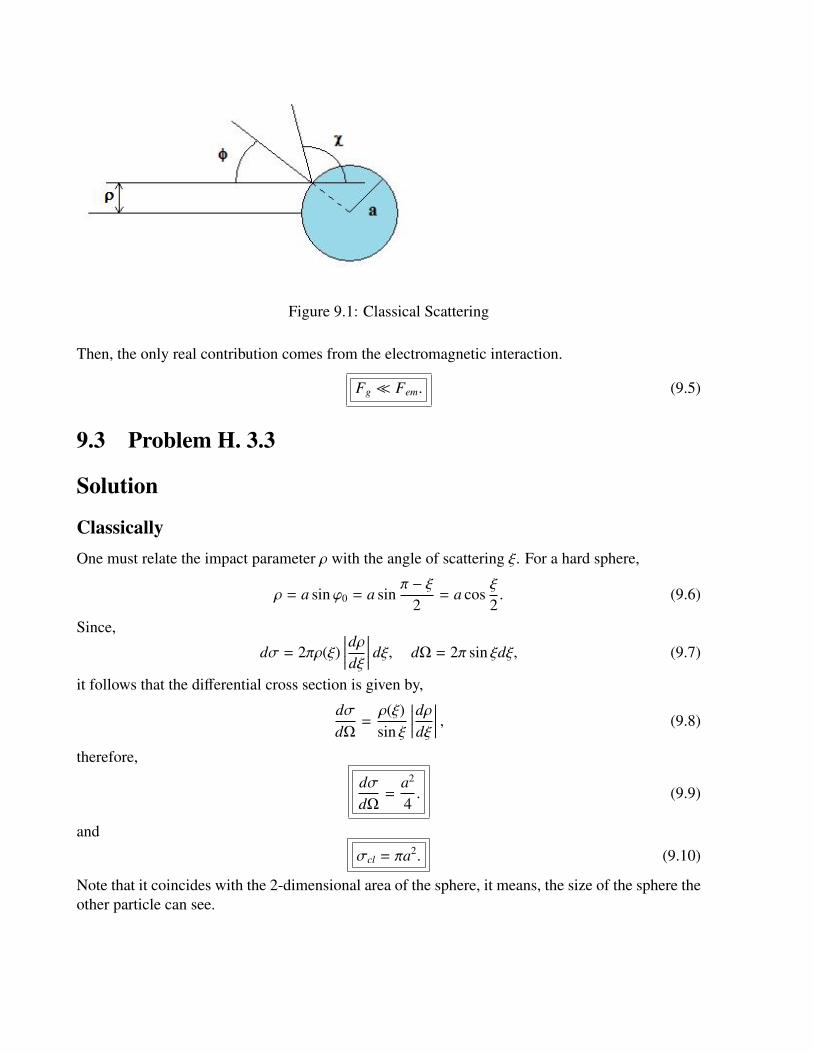
Figure 9.1: Classical Scattering

Then, the only real contribution comes from the electromagnetic interaction.

Fg Fem. (9.5)

9.3 Problem H. 3.3

Solution

ClassicallyOne must relate the impact parameter ρ with the angle of scattering ξ. For a hard sphere,

ρ = a sinϕ0 = a sinπ − ξ

2= a cos

ξ

2. (9.6)

Since,

dσ = 2πρ(ξ)∣∣∣∣∣dρdξ

∣∣∣∣∣ dξ, dΩ = 2π sin ξdξ, (9.7)

it follows that the differential cross section is given by,

dσdΩ=ρ(ξ)sin ξ

∣∣∣∣∣dρdξ

∣∣∣∣∣ , (9.8)

therefore,

dσdΩ=

a2

4. (9.9)

and

σcl = πa2. (9.10)

Note that it coincides with the 2-dimensional area of the sphere, it means, the size of the sphere theother particle can see.

QuantumA hard sphere is a scattering potential described by

V(r) =∞;r < R0 ;r > R . (9.11)

Thus,Al(r)|r=R = 0 =⇒ jl(kR) cos δl = nl(kR) sin δl, (9.12)

or

tan δl =jl(kR)nl(kR)

. (9.13)

Consider just l = 0, which represents an S -wave scattering, so

tan δ0 =sin(kR)/kR− cos(kR)/kR

= − tan kR, (9.14)

orδ0 = −kR. (9.15)

The radial wave function (with the eıδ omitted),

Al=0(r) ∝sin kr

krcos δ0 +

cos(kr)kr

sin δ0 =1kr

sin(kr + δ0). (9.16)

Low energy limit

For kR 1, the asymptotic expansions of the spherical functions are

jl(kr) '(kr)l

(2l + 1)!!, (9.17)

nl(kr) ' −(2l − 1)!!

(kr)l+1 . (9.18)

Then,

tan δl ' −(kR)2l+1

(2l + 1)[(2l − 1)!!]2 , (9.19)

and finally,

dσdΩ=

sin2 δ0

k2 ' R2, (9.20)

and

σnr = 4πR2. (9.21)

Ultra-relativistic limit

In this limit, lmax ' kR. Then,

σur '4πk2

l'kR∑l=0

(2l + 1) sin2 δl, (9.22)

but

in2δl =tan2 δl

1 + tan2 δl=

j2l (kR)

j2l (kR) + n2

l (kR)≈ sin2

(kR −

πl2

), (9.23)

because,

jl(kR) ∼1

kRin

(kR −

lπ2

)and

nl(kR) ∼ −1

kRcos

(kR −

lπ2

).

Finally,

σur =4πk2 (kR)2 1

2= 2πR2. (9.24)

9.4 Problem H. 4.1Describe an experimental method for the verification of the Maxwell-Boltzmann distribution.

SolutionA plausible experiment is the mean distribution of velocities of a gas expelled from a volumethrough a small hole.

The number of atoms per unit volume moving in the normal direction to the wall is

dn = n f (v)v2dv sin θdθdϕ, (9.25)

where n is the number density and f is the speed distribution.So, for The total atomic flow rate, R, through the hole is given by

R = 2πnA∫ ∞

0f (v)v3dv

∫ π/2

0sin θ cos θdθ = πAn

∫ ∞

0f (v)v3dv, (9.26)

orR =

An4〈v〉 . (9.27)

This is highly dependent on f (v), so one can check the Maxwell-Boltzmann distribution.

Figure 9.2: Gas enclosed on a box is escaping very slowly, so the process is almost in equilibrium.

NOTE: This is indeed the way neutrons (or other neutral particles) are accelerated, because thereis not possibility of applying electric fields.

9.5 Problem H. 4.5Estimate the probability that a 7 cents airmail stamp (mass=0.1 g) resting on a desk top at roomtemperature (300 K) will spontaneously fly up to a height of 10−8cm above the desktop.

SolutionSo, one can use the canonical ensemble, i.e.,

Pr =e−βεr∑s e−βεs

. (9.28)

The energy involved is just the gravitational potential energy, mgh. In CGS units,k = 1.38 ∗10−16erg/K, the gravitational acceleration is g = 103cm/s2, so an estimation is

Pr ≈ e−mghkT ∼ e

−10−110310−8

10−16102 = e−108. (9.29)

In this thick approximation, the exponent is so huge that changing the base from e to 10 is allowed,thus

Pr ∼ 10−108. (9.30)

This is barely non zero.

9.6 Problem H. 4.6A room of volume 3 × 3 × 3 cubic meters is under standard conditions

1. Estimate the probability that at any instant of time a 1cc volume anywhere within this roombecomes totally devoid of air because of spontaneously statistical fluctuations.

2. Estimate the same for 1A3 volume.

SolutionOnce more, one can use the canonical ensemble, but since p and T are given, one can use the idealgas equation of states and rewrite the probability in terms of V ,

Pv ∼ e−N vV . (9.31)

In the room the number of particles is of order N ' 1026, the volumes are va = 1cm3, vb =

1A3 = (10−8cm)3 = 10−24cm3 and V = 27 ∗ 106cm3, then

Pa ∼ e−1026

106 = e−1020, (9.32)

whilst

Pb ∼ e−102610−24

106 = e−10−8. (9.33)

From (9.32) one conclude that the probability is barely different than zero, but (9.33) is rela-tively 1.

9.7 Problem H. 4.7Suppose the situation referred to in Problem 9.6 first part has occurred. Describe qualitatively thebehavior of the distribution function thereafter. Estimate the time it takes for the situation to occuragain, under the assumption that molecular collisions are such that time sequence of the state ofthe system is a random sequence of states.

SolutionAfter the state in which a cubic centimeter has been devoid, the gas will suffer a free expansion andthe vacuum will be occupied.

Since the average time of collisions is of order ∆t ∼ 10−11s, then the time in which the situationwill be repeated is given by

t =∆tPa∼ 10−11s ∗ e1020

∼ 101020s. (9.34)

NOTE: The larger estimated age of the universe is 20 billion year (tu ∼ 1020s, but t tu. Thismeans that if the situation is reached, the probability of seeing it again could be considered zero.

9.8 Problem H. 4.9Let

H =∫

d3v f (~v, t) ln f (~v, t), (9.35)

where f (~v, t) is arbitrary except for the conditions∫d3v f (~v, t) = n and

∫d3v

12

mv2 f (~v, t) = ε. (9.36)

Show that H is minimum when f is the Maxwell-Boltzmann distribution.

SolutionIn order to extremize the functional H constrained to (9.36), one can use Lagrange multipliers.Then,

HT =

∫d3v

[f ln f + α f +

βmv2

2f + cont.

], (9.37)

whose variation yields

(δ f ) ln f + f δ ln f + αδ f +βm2δ(v2) f +

βmv2

2δ f = 0. (9.38)

Sinceδ f =

∂ f∂~v· δ~v, (9.39)

then [∂ f∂~v

ln f +∂ f∂~v+ α

∂ f∂~v+ βm~v f +

βmv2

2∂ f∂~v

]· δ~v = 0. (9.40)

But the variation of ~v is arbitrary, and the equation can be written like

~∇v f(1 + α +

βmv2

2+ ln f

)= −βm~v f . (9.41)

In principle the solution of this equation is known if the term inside the bracket is one. More-over, the restriction of the bracket is also solution of the complete equation. Thus,

f (~v, t) = e−αe−βm~v2

2 . (9.42)

This is nothing but the Maxwell-Boltzmann distribution.

9.9 Problem H. 5.1Make order-of-magnitude estimates for the mean free path and the collision time for

a.- H2 molecules in standard conditions (diameter H2 = 2.9A)

b.- A proton in a plasma at T = 3 ∗ 105K, n = 1015 particles/cc, σ = πr2, where r =e2

kT.

c.- A proton as before but T = 107K, where thermonuclear reaction occur.

d.- A proton in the sun’s corona, T = 106K and n = 106 protons/cc.

e.- slow neutrons with E = 0.5MeV in U238 (σ ≈ πr2, r ≈ 10−13cm)

SolutionThe mean-free path is given by

λ =14

√π

21

nσ, (9.43)

and the collision time is

τ =14

√π

21

nσv. (9.44)

Then, the task is finding the values of σs, ns and vs.In CGS units,

e2

kT=

1.5 ∗ 10−7

Tcm, (9.45)

Then,

ra ∼ 10−8cm,rb ∼ 10−12cm,rc ∼ 10−14cm,rd ∼ 10−12cm,re ∼ 10−13cm. (9.46)

So, σs are given by (πr2)

σa ∼ 10−15cm2,

σb ∼ 10−23cm2,

σc ∼ 10−27cm2,

σd ∼ 10−23cm2,

σe ∼ 10−25cm2. (9.47)

Since v =

√2kTm= 4.19 ∗ 107

(me

mi

)1/2

T 1/2cm/s, it follows that,

va ∼ 107cm/s,vb ∼ 108cm/s,vc ∼ 109cm/s,vd ∼ 108cm/s,ve ∼ 109cm/s. (9.48)

Thus,

λa ∼ 10−16cm,λb ∼ 108cm,λc ∼ 1012cm,λd ∼ 1019cm,λe ∼ 10−18cm, (9.49)

and

τa ∼ 10−23s,τb ∼ 100s,τc ∼ 103s,τd ∼ 1011s,τe ∼ 10−27s, (9.50)

9.10 Problem H. 5.4Show that the velocity of sound in a real substance is to a good approximation given by cs =

1/√ρκs, where ρ is the mass density and κsis the adiabatic compressibility, by the following steps:

(a) Show that in a sound wave the density oscillates adiabatically if K csλρCV , where

cs = velocity of soundλ = wave lengthρ = mass density

CV= specific heatK = Coefficient of thermal conductivity.

(b) Show by numerical examples, that the criterion stated in (a) is well satisfied in most practicalsituations.

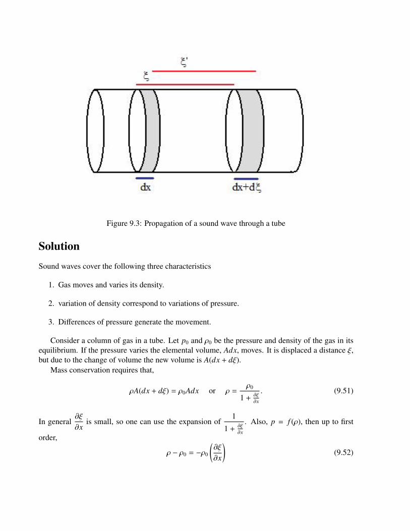
Figure 9.3: Propagation of a sound wave through a tube

Solution

Sound waves cover the following three characteristics

1. Gas moves and varies its density.

2. variation of density correspond to variations of pressure.

3. Differences of pressure generate the movement.

Consider a column of gas in a tube. Let p0 and ρ0 be the pressure and density of the gas in itsequilibrium. If the pressure varies the elemental volume, Adx, moves. It is displaced a distance ξ,but due to the change of volume the new volume is A(dx + dξ).

Mass conservation requires that,

ρA(dx + dξ) = ρ0Adx or ρ =ρ0

1 + ∂ξ

∂x

. (9.51)

In general∂ξ

∂xis small, so one can use the expansion of

1

1 + ∂ξ

∂x

. Also, p = f (ρ), then up to first

order,

ρ − ρ0 = −ρ0

(∂ξ

∂x

)(9.52)

and

p = p0 + (ρ − ρ0)(dpdρ

)0+ · · · = p0 − ρ0

(∂ξ

∂x

) (dpdρ

)0. (9.53)

Further, the equation of motion requires the acceleration∂2ξ

∂t2 ,so a little algebra yields

∂2ξ

∂t2 =

(dpdρ

)0

∂2ξ

∂x2 , (9.54)

then

c2s =

(dpdρ

)0. (9.55)

Now, the coefficient of thermal conductivity is defined as the flux energy through unit areadivided by the gravient of temperature, so

K =1A

dEdt

dzdT=

1A

dEdT

dzdt' CVcsρλ, (9.56)

then for an adiabatic process, one must requires

K CVλρcs, (9.57)

because the transference of heat should be zero. In this case,

pVγ = cte, (9.58)

and, for an ideal gas,

κS = −1V

(∂V∂p

)S= −

1V

1∂p∂V

S

=1γp. (9.59)

Moreover, the adiabatic relation of p and ρ is p = cteργ, thus

c2s =

γpρ=

1κS, (9.60)

finally,

cs =

√1ρκS

. (9.61)

Since CV ∼ 1.4, cs ∼ 3 ∗ 104cm/s, λ ∈ [1.5, 1500] and ρ ≥ 1, then in all cases showed in thetable, K CVcsρλ is satisfied.

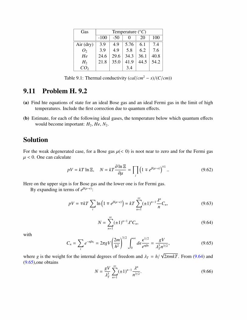
Gas Temperature (oC)-100 -50 0 20 100

Air (dry) 3.9 4.9 5.76 6.1 7.4O2 3.9 4.9 5.8 6.2 7.6He 24.6 29.6 34.3 36.1 40.8H2 21.8 35.0 41.9 44.5 54.2

CO2 3.4

Table 9.1: Thermal conductivity (cal/cm2 − s)/(C/cm))

9.11 Problem H. 9.2(a) Find hte equations of state for an ideal Bose gas and an ideal Fermi gas in the limit of high

temperatures. Include the first correction due to quantum effects.

(b) Estimate, for each of the following ideal gases, the temperature below which quantum effectswould become important: H2, He, N2.

SolutionFor the weak degenerated case, for a Bose gas µ(< 0) is noot near to zero and for the Fermi gasµ < 0. One can calculate

pV = kT lnΞ, N = kT∂ lnΞ∂µ

=∏

i

(1 ∓ eβ(µ−ε)

)∓1.. (9.62)

Here on the upper sign is for Bose gas and the lower one is for Fermi gas.By expanding in terms of eβ(µ−ε):

pV = ∓kT∑

i

ln(1 ∓ eβ(µ−ε)

)= kT

∞∑n=1

(±1)n−1λn

nCn, (9.63)

N =∞∑

n=1

(±1)n−1λnCn, (9.64)

with

Cn =∑

i

e−nβεi = 2πgV(2mh2

)3/2 ∫ ∞

0dεε1/2

enβε =gV

λ3T n3/2

, (9.65)

where g is the weight for the internal degrees of freedom and λT = h/√

2πmkT . From (9.64) and(9.65),one obtains

N =gVλ3

T

∞∑n=1

(±1)n−1 λn

n3/2 . (9.66)

Assuming the power series in x = Nλ3T/gV for λ = a1x + a2x2 + a3x3 + · · · , one can determine

the coefficients successively from (9.66),

a1 = 1, a2 = ∓1

23/2 , a3 =14−

(13

)3/2

, · · · (9.67)

Substituting this values of λ into (9.63), one get

pvkT= 1 −

1

4√

2

(λ3

T

v

)+

(18−

2

9√

3

) (λ3

T

v

)2

− · · · . (9.68)

9.12 Problem H. 9.3Pair correlation function: The pair correlation function D(~r1,~r2) of a system of particles isdefined as the probability of simultaneously finding a particle in the volume d~r1 about ~r1 and aparticle in the volume d~r2 about ~r2.

Calculate D(~r1,~r2) for an ideal Bose gas and an ideal Fermi gas in the limit of High tempera-tures. Include quantum corrections only to the lowest approximation.

SolutionClassically one has,

D(~r1,~r2) =N(N − 1)

∫d3N pd3r3 · · · d3rNe−βH(p,r)∫

d3N pd3Nre−βH(p,r). (9.69)

In order to include the lowest quantum corrections, one can replace the free Hamiltonian by

H(p, r) =∑

i

p2i

2m+

∑i< j

vi j. (9.70)

Assume that the density the gas is almost zero. The limit N → ∞, V → ∞ should be so takenthat N/V → 0. Then,

D(~r1,~r2) =N(N − 1)VN−2

[1 ± f12

2 ±N(N − 1)

2V

∫d3 f 2(r)

]1 ±

N(N − 1)2V

∫d3 f 2(r)

≈1v2

[1 ± exp

(−

2πλ2

∣∣∣~r1 − ~r2

∣∣∣2)] . (9.71)

This result continues to hold for finite v with λ3/v 1, although the derivation did not justifysuch a conclusion.

9.13 Problem H. 9.5

Consider the grand partition function

Q(z,V) = (1 + z)V(1 + zαV), (9.72)

where α is a positive constant.

(a) Write down the equation of state in the parametric for, eliminate z graphically, and show thatthere is a first-order phase transition. Find the specific volumes of the two phases.

(b) Find the roots of Q(z,V) = 0 in the complex z plane, at fixed V . Show that as V → ∞the rootconverge toward the real axis at z = 1.

(c) Find the equation of state in the “gas” phase. Show that a continuation of this equation beyondthe phase transition density fails to show any sign of the transition. This will demonstratethat the order of the operations z

(∂∂z

)and V → ∞ can be interchanged only within a single

phase region.

Solution

The parametric equation of state are

pkT

= ln(1 + z) +1V

ln(1 + zαV), (9.73)

1v=

z1 + z

+ αzαV

1 + zαV . (9.74)

The roots of Q are z = −1 which does not belong to the physical system, and zαV = −1. Thislast, so that z is unimodular, can be written as

z = eıθ ⇒ ıθαV = ±π, (9.75)

or

ıθ = ±π

αV. (9.76)

It is clear that in the limit V → ∞, in order to preserve the relation, θ → 0, thus

z→ 1. (9.77)

9.14 Problem H. 11.1

Give the numerical estimates for the Fermi energy of

(a) e− in a typical metal,

(b) nucleons in a heavy nucleus,

(c) He3 atoms in liquid He3 (atomic volume = 46.2A3/atom).

Treat all of the mentioned particles as free particles.

Solution

Since

εF =h2

2m

(3n

4π(2σ + 1)

)2/3

, (9.78)

then, for electrons in a metal, whose n = 5.86 ∗ 1028elect/m3, it follows that (σ = 1/2)

εF = 9 ∗ 10−19J ' 5.6eV. (9.79)

For a nucleon (with energyE = .5MeV) on a heavy nucleus, n ' 1030nucleon/cm3, mn ∼

10−30g, then

εF ∼ 10−3erg ∼ 10−10J ∼ 1GeV. (9.80)

For He3, n ≈ 1022atoms/cm3, thus

εF ∼ 10−10erg ∼ 10−17J ∼ 100eV. (9.81)


Show that for the ideal gas of N particles the Helmholtz energy at low temperatures is given by

AN=

35εF

1 − 5π2

12

(kTεF

)2

+ · · ·

. (9.82)

Solution

It was shown that at low temperatures the energy is given by

U =35εF

1 + 5π2

12

(kTεF

)2

+ · · ·

= 35εF N. (9.83)

Moreover,

F = Nµ − pV = Nµ −23

U =35

NεF

1 − 5π2

12

(kTεF

)2

+ · · ·

, (9.84)

thus,

AN=

35εF

1 − 5π2

12

(kTεF

)2

+ · · ·

. (9.85)


Show that the equation of state of the ideal Bose gas in the gas phase can be written in the form ofthe Virial expansion

pvkT= 1 −

1

4√

2

(λ3

T

v

)+

(18−

2

9√

3

) (λ3

T

v

)2

− · · · (9.86)

Solution

See (9.68)


Consider a square lattice of Ising spins in any dimension, with energy given by

Eisi = −ε∑

sis j − HN∑

i=1

si. (9.87)

Show that in the absence of an external field (H = 0), the free energy at a given temperature is thesame for the ferromagnetic case (ε > 0) and the anti-ferromagnetic case (ε < 0).

Solution

Consider any lattice site designate it as a site of sub-lattice A. Designate it nearest neighbors assites belonging to sub-lattice B. The sub-lattices are completely defined by the rule that the nearestneighbors of any site in sub-lattice B are sites of sub-lattice A, and vice versa. In a square lattice,the nearest neighbors are situated on lattice spacing away, along mutually orthogonal directions.Therefore both A and B are square lattices. Denote the spin variables in sub-lattice A by sAi ,and those in sub-lattice B by sBi . Only spins in different sub-lattices interact. Thus, the partitionfunction can be written in form

Q =∑sA

∑sB

eJ∑ sAi sB j , (9.88)

where J = βε. Since sA is being summed over, the above is invariant under sAi → −sAi . Thereforeit is invariant under ε → −ε.

NOTE: the proof fails for a triangular lattice.


Duality of 2-dimensional Ising model.

(a) Let Q(N, β) denote the partition function for a 2-dimensional Ising model of N sites on a squarelattice at temperature kT = 1

βwith no external field. Show that in the limit N → ∞

ln Q(N, β)N

=ln Q(N, β∗)

N− sinh (2β∗) , (9.89)

where β∗ = − 12 ln tanh β, or

sinh 2β sinh 2β∗ = 1. (9.90)

Note that β∗ is a decreasing function of β. Thus, the high temperature properties of the systemare explicitly related to its low temperature properties.

(b) One know through Peierls argument that the system exhibits spontaneous magnetization. As-suming that the critical temperature Tc is unique, one conclude βc = β

∗c. Show

βc =12

ln(1 +√

2). (9.91)

This is how the transition temperature of the 2-dimensional Ising model was obtained beforeOnsager’s explicit solution.

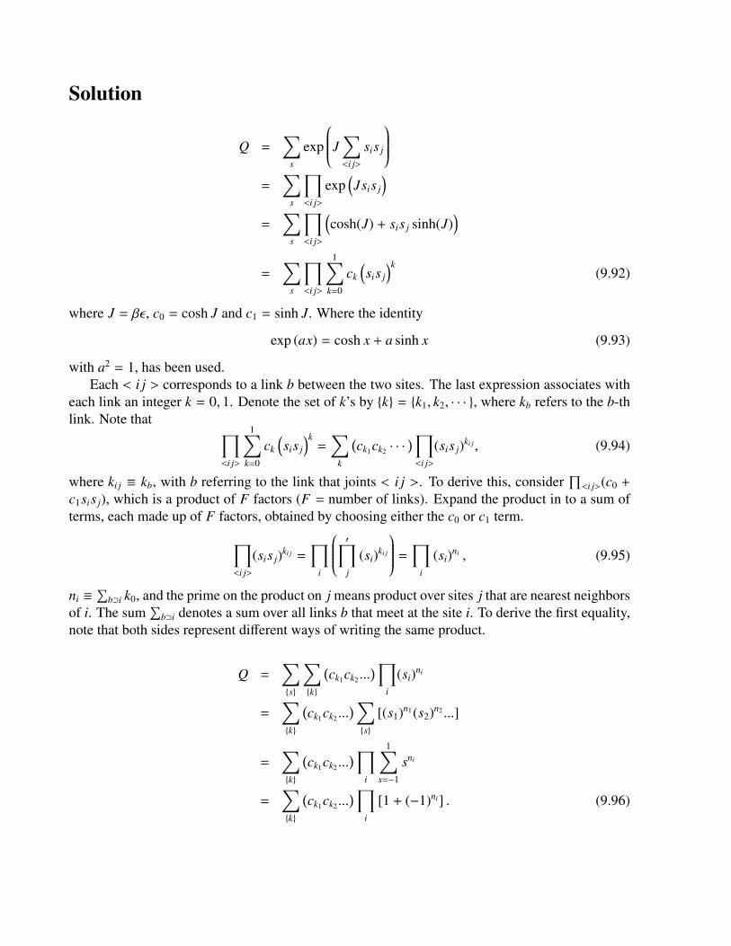
Solution

Q =∑

s

exp

J∑

sis j

=

∑s

∏

exp(Jsis j

)=

∑s

∏

(cosh(J) + sis j sinh(J)

)=

∑s

∏

1∑k=0

ck

(sis j

)k(9.92)

where J = βε, c0 = cosh J and c1 = sinh J. Where the identity

exp (ax) = cosh x + a sinh x (9.93)

with a2 = 1, has been used.Each corresponds to a link b between the two sites. The last expression associates with

each link an integer k = 0, 1. Denote the set of k’s by k = k1, k2, · · · , where kb refers to the b-thlink. Note that ∏



1∑k=0

ck

(sis j

)k=

∑k

(ck1ck2 · · ·

)∏

(sis j)ki j , (9.94)

where ki j ≡ kb, with b referring to the link that joints . To derive this, consider∏

(c0 +

c1sis j), which is a product of F factors (F = number of links). Expand the product in to a sum ofterms, each made up of F factors, obtained by choosing either the c0 or c1 term.∏



(sis j)ki j =∏

i

′∏j

(si)ki j

=∏i

(si)ni , (9.95)

ni ≡∑

b⊃i k0, and the prime on the product on j means product over sites j that are nearest neighborsof i. The sum

∑b⊃i denotes a sum over all links b that meet at the site i. To derive the first equality,

note that both sides represent different ways of writing the same product.

Q =∑s

∑k

(ck1ck2 ...

)∏i

(si)ni

=∑k

(ck1ck2 ...

)∑s

[(s1)n1(s2)n2 ...]

=∑k

(ck1ck2 ...

)∏i

1∑s=−1

sni

=∑k

(ck1ck2 ...

)∏i

[1 + (−1)ni] . (9.96)

Note [1 + (−1)ni] = 0 for ni odd, 2 for ni even. Since ni depends on kb, only that subset of kb

corresponding to all ni even will contribute:

Q = 2N′∑k

(ck1ck2 ...

), (9.97)

where the prime on the sum denotes the constraint∑

b⊃i kb = 0 (mod 2), for all i.That is, associated with each link b and integer kb = 0, 1, such that k1 + ... + k4 = 0 (mod 2)

whenever the links 1, 2, 3, 4 all meet at one site.One solve the constraint through a geometrical construction. Define the “dual lattice” as the

lattice whose sites are located at centers of each square of the original lattice. In the accompanyingsketch, the dual lattice sites are marked with an x, and the links of the dual lattice are shown dotted.each original site i is contained in a square of the dual lattice, which is called a “plaquette”. Attachto each site of the dual lattice a dual spin variable, σi, which can assume only the values ±1. If 1,2, 3, 4 are dual sites at successive corners of a plaquette (say in clock-wise order), then

σ1σ2 + σ2σ3 + σ3σ4 + σ4σ1 = 0 (mod 4) (9.98)

to see this, note that the left side can be written in the form (σ1 + σ3)(σ2 + σ4) = 0,±4. Noe eachlink b of the original lattice cuts a unique link b∗ of the dual lattice. The constraint is solved bytaking

kb =12

(1 − σ1σ2) (9.99)

where 1, 2 mark the dual sites at the ends of b∗. This is so because, first, kb = 0, 1 as required, andsecond whenever 4 links meet at the same site, they cut the sides of the plaquette containing thesite. One know in passing that an equally acceptable definition of kb can be obtained by changingthe − → +. This shows that in this case the ferromagnetic model and the anti-ferromagnetic modelhave the same free energy, in agreement with the general theorem stated in the last problem.

Since there is a one-to-one correspondence between links on the original and on the dual lattice,ona can associated with a dual link b∗ the integer kb∗ ≡ kb. For large N, the number of dual sites isalso N. One can associate each dual site with 2 dual links (say, the once pointing north and east).There are 2N integers kb∗ , of which N are independent (because they satisfy N constraints). Thus,the partition function is obtained by replacing the constraint sum

∑′k by the un-constraint sum

12

∑σ:

Q = 2N−1∑σ

(ck1ck2 ...

)(9.100)

where the c’s are to be re expressed in terms of the σ ’s.

ck = k sinh J + (1 − k) cosh J

=12

(1 − σ1σ2) sinh J +12

(1 + σ1σ2) cosh J

=12

eJ(1 + σ1σ2e−2J

)=

12

eJ (1 + σ1σ2 tanh J∗) (9.101)

Figure 9.4: Dual lattice

where J∗ tanh J∗ ≡ e−2J is defined, with a view to re expressing the above expression as an expo-nential:

ck =eJ

2 cosh J∗(cosh J∗ + σ1σ2 sinh J∗)

= [2 sinh(2J)]−1/2 exp (J∗σ1σ2) . (9.102)

Thus, finally

Q =12

(sinh 2J∗)−N∑σ

exp

J∗∑

σiσ j

. (9.103)

9.19 Problem G.-C. 6.1Show that the number of particles in a Fermi gas with celerity between [vz, vz+dvx] (or its equivalentin momentum) is

n(pz)dpz =

(2πm(2σ + 1)V

βh3

)ln

[β

(µ −

p2z

2m

)− 1

]. (9.104)

Find the limit of this expression when T → 0.

SolutionFor a Fermi gas,

n(~p) =(2σ + 1)V

h3

1

e−β(

p22m−µ

)+ 1

, (9.105)

then in cylindric coordinates,

n(~p)d3 p =(2σ + 1)V

h3

prdpr pzdθ

e−β

(p2

r +p2z

2m −µ

)+ 1

. (9.106)

Next, one should integrate the angular and radial components of the momentum. By using theintegral identity ∫

dxa + bemx =

1am

[mx − ln(a + bemx)] , (9.107)

one gets

n(pz)dpz =4π(2σ + 1)mV

βh3 ln

eβ(

p2z

2m−µ

)+ 1

dpz. (9.108)

Finally, for T → 0⇒ e1/T → ∞, ∴ ln

eβ(

p2z

2m−µ

)+ 1

→ p2z

2m − µ. Thus,

n(pz)dpz →4π(2σ + 1)mV

h3

(p2

z

2m− µ

)dpz. (9.109)

9.20 Problem G.-C. 6.5Show that ex/(1 + ex)2 is a symmetric function on x, and that it goes to zero as long as x→ ±∞.

SolutionUnder parity transformation,

ex

(1 + ex)2 7→e−x

(1 + e−x)2 =e−x

e−2x(ex + 1)2 =ex

(1 + ex)2 . (9.110)

Then,f (x) = f (−x). (9.111)

Now,

f (±∞) =e±∞

(1 + e±∞)2 =

0/1 ;x→ −∞

e+∞e2∞ → 0;x→ +∞

(9.112)

Therefore, this equation goes to zero as x→ ±∞.

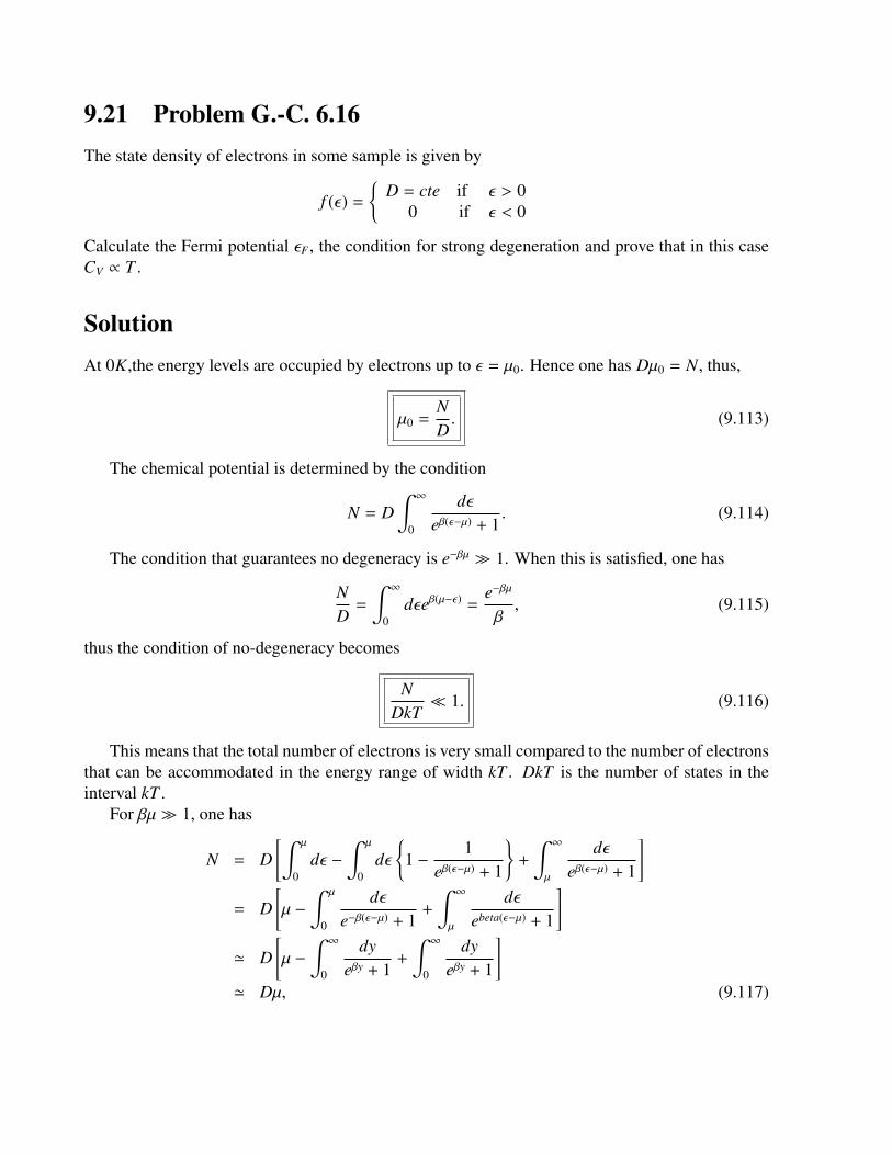
9.21 Problem G.-C. 6.16The state density of electrons in some sample is given by

f (ε) =

D = cte if ε > 00 if ε < 0

Calculate the Fermi potential εF , the condition for strong degeneration and prove that in this caseCV ∝ T .

SolutionAt 0K,the energy levels are occupied by electrons up to ε = µ0. Hence one has Dµ0 = N, thus,

µ0 =ND. (9.113)

The chemical potential is determined by the condition

N = D∫ ∞

0

dεeβ(ε−µ) + 1

. (9.114)

The condition that guarantees no degeneracy is e−βµ 1. When this is satisfied, one has

ND=

∫ ∞

0dεeβ(µ−ε) =

e−βµ

β, (9.115)

thus the condition of no-degeneracy becomes

NDkT

1. (9.116)

This means that the total number of electrons is very small compared to the number of electronsthat can be accommodated in the energy range of width kT . DkT is the number of states in theinterval kT .

For βµ 1, one has

N = D[∫ µ

0dε −

∫ µ

0dε

1 −

1eβ(ε−µ) + 1

+

∫ ∞

µ

dεeβ(ε−µ) + 1

]= D

[µ −

∫ µ

0

dεe−β(ε−µ) + 1

+

∫ ∞

µ

dεebeta(ε−µ) + 1

]' D

[µ −

∫ ∞

0

dyeβy + 1

+

∫ ∞

0

dyeβy + 1

]' Dµ, (9.117)

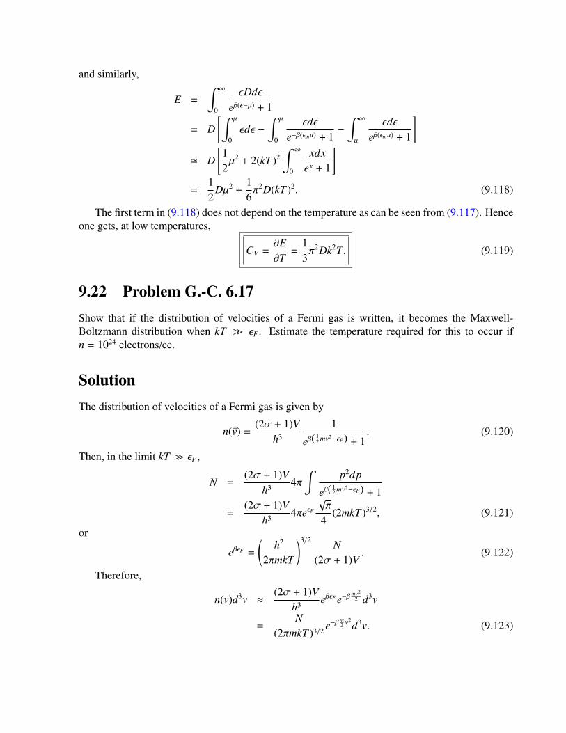
and similarly,

E =

∫ ∞

0

εDdεeβ(ε−µ) + 1

= D[∫ µ

0εdε −

∫ µ

0

εdεe−β(εmu) + 1

−

∫ ∞

µ

εdεeβ(εmu) + 1

]' D

[12µ2 + 2(kT )2

∫ ∞

0

xdxex + 1

]=

12

Dµ2 +16π2D(kT )2. (9.118)

The first term in (9.118) does not depend on the temperature as can be seen from (9.117). Henceone gets, at low temperatures,

CV =∂E∂T=

13π2Dk2T. (9.119)

9.22 Problem G.-C. 6.17Show that if the distribution of velocities of a Fermi gas is written, it becomes the Maxwell-Boltzmann distribution when kT εF . Estimate the temperature required for this to occur ifn = 1024 electrons/cc.

SolutionThe distribution of velocities of a Fermi gas is given by

n(~v) =(2σ + 1)V

h3

1

eβ(12 mv2−εF) + 1

. (9.120)

Then, in the limit kT εF ,

N =(2σ + 1)V

h3 4π∫

p2dp

eβ(12 mv2−εF) + 1

=(2σ + 1)V

h3 4πeεF

√π

4(2mkT )3/2, (9.121)

or

eβεF =

(h2

2πmkT

)3/2 N(2σ + 1)V

. (9.122)

Therefore,

n(v)d3v ≈(2σ + 1)V

h3 eβεF e−βmv2

2 d3v

=N

(2πmkT )3/2 e−βm2 v2

d3v. (9.123)

Equation (9.123) is the same as the Maxwell-Boltzmann distribution.

9.23 Problem G.-C. 7.15For massive particles, pV = 2

3U. In the case of photons as massless particles whose momentum isp = hν

c , show that p = 13u. Explain the difference between them.

SolutionThe Helmholtz free energy F(= Nµ − pV) of the photon gas is equal to −pV because µ = 0.

On the other hand, the grand partition function is

pV = kT lnΞ = −kT∑

i

ln(1 − e−βhνi

). (9.124)

The energy spectrum of the photon gas is given by E(k) = hck, k is the modulo of the wave vector.Then, the summation over i is to be interpreted as that over the wave vector ~k, and this can bereplaced by an integral. Taking into account the weight 2 which comes from the two differentpolarizations of the photon, one obtains

pV = −kT∫ ∞

0ln

(1 − e−β~cq

) 2 ∗ 4πV(2π)3 q2dq

= −(kT )4Vπ2(~c)3

∫ ∞

0ln

(1 − e−x) x2dx

=(kT )4V

3π2(~c)3

∫ ∞

0ln

(1 − e−x) x3dx, (9.125)

after integration by parts.The integral in (9.125) turns to have the value π4/15.Hence,one has, finally

pV = −F =Vπ2(kT )4

45(~c)3 =4σV3c

T 4, (9.126)

with σ the Stefan-Boltzmann constant. The entropy is given by

S =16σV

3cT 3, (9.127)

thenU(= F + TS ) =

4σVc

T 4. (9.128)

Thus,

p =u3. (9.129)

9.24 Problem G.-C. 7.16Suppose that sun emits electromagnetic waves from its surface (T ∼ 106K) calculate the pressureexerts by that radiation. How is it compared with the one of a mol of ideal gas enclose on a volumeof 1cm3?

SolutionIn SI units, σ = 5.67 ∗ 10−8Jm−2K−4s−1, R = 8.315J/K ∗ mol and c = 3 ∗ 108m/s.

From (9.129), it follows that

ps =u3=

4σ3c

T 4 = 2.52 ∗ 108J/m3. (9.130)

Similarly, from the ideal gas equation of states, it follows that

p(i) =8.315J/s ∗ 300K

10−6M3 = 2.5 ∗ 109J/m3. (9.131)

Then,p(i) ∼ 10ps. (9.132)

9.25 Problem G.-C. 7.20Show that an ideal boson gas on 2-D does not condensate.

SolutionThe energy levels of free particles in a 2-D region on Lx × Ly are given by

ε(kx, ky) =~2

2m(k2

x + k2y), (9.133)

with ki =2πniLi

and ni ∈ Z.One can use the formula which is established generally in the Bose-Einstein statistics, i.e.,

N =∑

i

1eβ(εi−µ) − 1

, (9.134)

where N is the total number of particles, µ is the chemical potential and summation is over all pos-sible energy levels. Assuming Li sufficiently large, one can replace this summations by integrationin the (kx, ky)-space,

N =LxLy

(2π)2 2π∫ ∞

0

kdk

eβ

~2k2

2m−µ

− 1

= 2πLxLymh2

∫ ∞

0

dεeβ(ε−µ) − 1

, (9.135)

or

N = LxLy2πmkT

h2

∞∑l=1

1le

lµkT . (9.136)

From (9.136), one knows that always is possible to get a value of µwhich is not of order 1/N.Henceone can conclude that there are no levels which are occupied by a number of molecules of order N,so that Bose-Einstein condensation does not occur.

9.26 Problem G.-C. 7.21Photons obey Bose-Einstein statistics, so, one would assure that a photon gas condense. Is itcorrect? If this is correct, calculate Tc.

SolutionElectromagnetic waves confined in a container can be regarded as superpositions of normal modeof oscillations.

Let νi be the frequency of the i-th normal mode and ni be the quantum of that mode which canbe treated as a quantized harmonic oscillator. Then,

E(n0, n1, · · · ) =∑

i

nihνi, (9.137)

is the energy of the electromagnetic wave which is in the quantum state specified by (n0, n1, · · · ).The zero point of energy is omitted by the adjustment of energy. By (9.137), one can consider

ni as the number of photons with energy hνi. Hence the canonical ensemble partition function forthis photon gas is given by

Z(T,V) =∞∑

n0=0

∞∑n1=0

· · · e−βE(n0,n1...) =∏

i

(1 − e−βhνi

)−1, (9.138)

and the average value of n j is given by

n j =1

e−βhν j − 1. (9.139)

One can interpret (9.138) as the grand partition function and (9.139) as the distribution functionfor an ideal gas with µ = 0 respectively.

Thus the condition µ ∼ kT is fulfilled just for T → 0 which is the critical temperature of thephoton gas.

9.27 Problem G.-C. 10.1

Obtain the equations mηr = −mω2rηr and H =

∑r

(p2

r2m +

mω2r

2 η2r

).

SolutionFor a solid, the equations of motion are given by a set of coupled harmonic oscillators,

mω2ξ j = −∑

i

Φi jξi. (9.140)

Nonetheless, one one can introduce a set of orthonormal basis vectors, a j, s.t. ξ j =∑

r a(r)j ηr are the

principal vectors of the potential Φ, e.i.,∑

iΦi ja(r)j = mω2

rδi ja(r)j .

Then, (9.140) yields, ∑r

a(r)j

(mηr + mω2

rηr

)= 0 ∀a(r)

j , (9.141)

thus,

mηr = −mω2rηr. (9.142)

Similarly, the Hamiltonian

H =3N∑i=1

p2i

2m+

12

3N∑i, j=1

Φi jξiξ j, (9.143)

becomes1, ∑i

p2i

2m=

m2

2m

∑i

∑rr′

a(r)i a(r′)

i ηrηr′

=1

2m

∑rr′δrr′mηrmηr′

=1

2m

∑r

p2r , (9.144)

and

12

∑i j

Φi jξiξ j =12

∑i j

∑rr′Φi ja

(r)i a(r′)

j ηrηr′

=12

∑i j

∑rr′

mω2rδi ja

(r)i a(r′)

j ηrηr′

=12

∑i

∑rr′

mω2r a(r)

i a(r′)i ηrηr′

=12

∑r

mω2rη

2r . (9.145)

1Since pi = mξi = m∑

r a(r)i ηr.

From (9.144) and (9.145) it follows that

H =∑

r

(p2

r

2m+

12

mω2rη

2r

). (9.146)

9.28 Problem G.-C. 10.2

a.- The energy levels of a 3D isotropic harmonic oscillator are given by εn = (n + 3/2)hν. Showthat the n-th level has degeneration 1

2 (n + 1)(n + 2).

b.- Calculate the partition function for N oscillators and relate the result with the Einstein modelof solids.

Solution

In a 3D harmonic oscillator, εn = (n + 3/2)~ω, where n = nx + ny + nz, so the degeneration is givenby the number of ways one can array n object in three different boxes.

The number of ways of distributing M white balls among N labeled boxes is equivalent to thepermutation of N−1 black balls in a row together with the white balls. Therefore, the combinatorialfactor is

gM =(M + N − 1)!M!(N − 1)!

. (9.147)

In the problem, M = n and N = 3, so

gn =12

(n + 1)(n + 2). (9.148)

The partition function is given by

Z1 =12

∑n

(n + 1)(n + 2)e−β(n+3/2)hν

=12

eβ12 hν

∑n

(n + 1)(n + 2)e−β(n+2)hν

=12

eβ12 hν

(−

∂

∂(βhν)

)∑n

(n + 1)e−β(n+2)hν

=12

eβ12 hν

(−

∂

∂(βhν)

)e−βhν

∑n

(n + 1)e−β(n+1)hν

=12

eβ12 hν

(−

∂

∂(βhν)

)e−βhν

(−

∂

∂(βhν)

)∑n

e−β(n+1)hν

=12

eβ12 hν

(−

∂

∂(βhν)

)e−βhν

(−

∂

∂(βhν)

)1

eβhν − 1

=12

eβ12 hν

(−

∂

∂(βhν)

)1

(eβhν − 1)2

=eβ

32 hν

(eβhν − 1)3 , (9.149)

or

ZN =eβ

3N2 hν

(eβhν − 1)3N . (9.150)

This yield the same results as the Einstein’s theory of crystals.

9.29 Problem G.-C. 10.3

a.- Use directly the definition of Debye’s function to showing

D(x) =

1 − 3x8 +

x2

20 + O(x3) ;x = θDT1

π4

5x3 − 3e−x(1 + O(1/x)); x 1(9.151)

b.- Use the above result to showing that

CV

Nk=

3[1 − 1

20 x2 + · · ·]

;x 1125 π

4 1x3

[1 − 15

4π x3e−x + · · ·];x 1

(9.152)

SolutionSince,

D(x) =3x3

∫ x

0

x3dxex − 1

, (9.153)

it follows that for x 1, ex − 1 ' x + x2

2! +x3

3! + · · · , then

∫ x

0dx

x2

1 + x + x2

2! +x3

3! + · · ·≈

∫ x

0dxx2

1 − (x2+

x2

3!+

x3

4!+ · · ·

)+

(x2+

x2

3!+

x3

4!+ · · ·

)2

+ · · ·

≈

∫ x

0dxx2 −

12

∫ x

0x3 +

112

∫ x

0dxx4 + · · ·

=x3

3−

x4

8+

x5

60+ · · · . (9.154)

Therefore,

D(x) ≈ 1 −3x8+

x2

20, for x 1. (9.155)

Similarly,for x 1 one get∫ x

0dx

x3

ex − 1=

∫ ∞

0dx

x3

ex − 1−

∫ ∞

xdx

x3

ex − 1

=π4

15−

∫ ∞

xdx

x3e−x

1 − e−x

=π4

15−

∫ ∞

xdxx3e−x

(1 + e−x + e−2x + · · ·

)≈

π4

15− x3e−x + · · · . (9.156)

Thus,

D(x) =π4

5x3 − 3e−x + O

(1x

). (9.157)

Moreover,U = U (D)

0 + 3NkT D(x), (9.158)

then, for x 1 yields,

CV = 3NkT −3

20Nk

(θD

T

)2

+ · · · = 3Nk(1 −

x2

20+ cdots

). (9.159)

And for x 1,

CV ≈125

NkTπ4(

TθD

)− 9Nke−

θDT + · · · , (9.160)

thus,CV

Nk=

125π4

(1x3

) [1 −

154π4 x3e−x + · · ·

]. (9.161)

9.30 Problem G.-C. 12.1

The measurement of polarization of an ideal gas is taken a 300K using an electric field of 2000V/m.Is it allowed to use L(x) = 1

3 x? Why? Assume µe = 2.64 Debyes.

Solution

Langevin’s function is definedby

L(x) = coth x −1x=

x3 +

x3

45 ; x < 11 ; x 1

(9.162)

with x = µeE/kT .In order to approximate Langevin’s function just like x/3, x 1.In the given set up, the condition x = 1 requires

Ec '1.38 ∗ 10−16 ∗ 300

3 ∗ 10−18 = 1.38 ∗ 104ues ' 4 ∗ 106V/m, (9.163)

since E Ec, then is valid taking the linear approximation.

9.31 Problem G.-C. 12.2

How would be modified the equation

κ − 14πn

= α +µ2

e

3kT,

if the first non-linear term of Langevin’s function is include? Under what conditions are usefullthis corrections?

SolutionSince

〈µe〉 = µeL(x), (9.164)

then,

〈µe〉 =µ2

eE3kT

(1 +

x2

15

). (9.165)

It follows that

P =n3µ2

eEkT

(1 +

x2

15

). (9.166)

If one includes the polarization of the molecules, hence,

χ = n[α +

µ2e

3kT

(1 +

x2

15

)]. (9.167)

Finally the electric displacement definition, yields

κ − 14πn

= α +µ2

e

3kT

(1 +

µ2eE2

15(kT )2

). (9.168)

This effect is not worthing unless one is interested in low temperatures and/or huge electricfields (order of MV/m).

9.32 Problem G.-C. 12.11Use the equation

CM = −2nJgµB

VσM[∂

∂TBσ

(bM

T

)]V, (9.169)

and the definition of the Brillouin to showing that CM = 0 when T → 0.

SolutionBy definition of the Brillouin function,

Bσ(BM/T ) = (σ + 1/2) coth[(σ + 1/2)

BMT

]−

12

coth(

BMT

). (9.170)

Since,∂

∂Tcoth(1/T ) ∝

1 − coth2(1/t)T 2 , (9.171)

when T → ∞, coth2(1/t)→ 1 exponentially, whilst the denominator explode potentially. Then,

CM → 0. (9.172)

as T → 0.

9.33 Problem G.-C. 15.1Show that the minimum work required to producing a fluctuation in entropy ∆S is precisely thenumerator of the argument of

Ω = C exp−∆E − T∆S I + p∆V − µ∆N

kT. (9.173)

SolutionUsing the thermodynamical relations for the total entropy S = S I + S II ,the fluctuation is given by

T∆S = ∆E − T∆S I + p∆V − µ∆N, (9.174)

then, one can write

Ω = C exp−∆Sk. (9.175)

Equation (9.175) is valid for the compose system I + II. Let the total system be transferredfrom the states A∗ into the state A∗ + A′, when the subsystem I is transferred from the state α∗ tothe state α∗ + α′, external work is being done.

Then, since whenever work is done the quasi-static (or reversible) way, it becomes minimum,one obtains

Wmin(α∗, α′) =∫ A∗+A′

A∗(dU − TdS ) , (9.176)

where U and S denote the energy and entropy of the composite system I + II, and T is the temper-ature at each intermediate stage of the process.

Since α is the change in a sufficiently small subsystem I one regards A′ as a very small deviationof the total system I + II, and therefore approximate T by the value T ∗ at the state A∗.

The composite system is supposes to be isolated, so the internal energy must be equal at bothstates. In this case,

Wmin(α∗, α′) = T ∗∆S . (9.177)

Finally

Ω(α∗, α′) = C exp(−

Wmin(α∗, α′)kT ∗

). (9.178)

9.34 Problem G.-C. 15.8Calculate the fluctuations of the square energy for Rayleigh-Jeans, Wien and Planck.

SolutionThe fluctuation of the energy square is given by⟨

E2(ν,T )⟩= hTV0dν

(∂u(ν,T )∂T

)V0

. (9.179)

Also, Rayleigh-Jeans energy density is

u(ν,T ) =8πν2

c3 kT,=⇒∂u∂T=

8πν2

c3 k. (9.180)

For Wien’s energy density,

u(ν,T ) = αν3e−βν/T ,=⇒∂u∂T=αβν4

T 2 e−βν/T . (9.181)

Finally for Planck’s energy density

u(ν,T ) =8πν3h

c3

1

ehνkT −1

,=⇒∂u(ν,T )∂T

=8πν4h2

c3kT 2

ehνkT

(ehνkT − 1)2

. (9.182)

If one uses the identity,

ehνkT

(ehνkT − 1)2

=1

ehνkT − 1

+1

(ehνkT − 1)2

, (9.183)

it follows directly that,

⟨E2(ν,T )

⟩=

u2(ν,T ) c3

8πν2 V0dν R.J.βkνV0u(ν,T )dν W.[

hνu(ν,T ) + c3

8πν2 u2(ν,T )]

V0dν Planck(9.184)

Part IV

Relativity

141

Chapter 10Relativity

10.1 Problem 1

Write down the line elements for

• A sphere of radius a, using the angles (θ, φ) as spherical coordinates.

• A cylinder whose transverse section is a circle of radius a, using (phi, z) as the coordinatesfor the cylinder. Is this cylinder plane or curved?

• A hyperbolic paraboloid, whose parametric equation is

~r = (u + v)ex + (u − v)ey + 2uvez, (10.1)

using the (u, v) parametrisation.

AnswerIn order to find the line element for each case, we just substitute the differentials of the line elementin terms of the new coordinates.

Spherical coordinatesThe change of basis is given by

x = a sin θ cos φ,y = a sin θ sin φ,z = a cos θ. (10.2)

143

then,

dx = a (cos θdθ cos φ − sin θ sin φdφ)dy = a (cos θdθ sin φ + sin θ cos φdφ)dz = −a sin θdθ, (10.3)

and

dx2 = a2(cos2 θ cos2 φdθ2 + sin2 θ sin2 φdφ2 − 2 sin θ cos θ cos φ sin φdθdφ

)dy2 = a2

(cos2 θ sin2 φdθ2 + sin2 θ cos2 φdφ2 + 2 sin θ cos θ cos φ sin φdθdφ

)dz2 = a2 sin2 θdθ2. (10.4)

Thus,ds2 = a2

(dθ2 + sin2 θdφ2

). (10.5)

Cylindric coordinates

For cylindric coordinates, the change of basis is given by

x = a cos φ,y = a sin φ,z = z. (10.6)

Then

dx = −a sin φdφdy = a cos φdφdz = dz, (10.7)

and

dx2 = a2 sin2 φdφ2

dy2 = a2 cos2 φdφ2

dz2 = dz2. (10.8)

Thusds2 = a2dφ + dz2. (10.9)

We note that a cylinder is a direct product R × S 1 this embedded is plane in R3.

Hyperbolic paraboloidFor hyperbolic paraboloid coordinates, the change of basis is given by

x = u + v,y = u − v,z = 2uv. (10.10)

Then

dx = du + dvdy = du − dvdz = 2vdu + 2udv, (10.11)

and

dx2 = du2 + dv2 + 2dudvdy2 = du2 + dv2 − 2dudvdz2 = 4v2du2 + 4u2dv2 + 8uvdudv. (10.12)

Thusds2 = (2 + 4v2)du2 + (2 + 4u2)dv2 + 8uvdudv. (10.13)

10.2 Problem 2Show that δµν has the expected tensorial character. Prove that δµν is a constant tensor which has thesame components in every coordinate frame. Evaluate δµµ and δµνδνµ.

AnswerLet us consider the change of coordinates xµ 7→ yµ, therefore, the matrix transformation is ∂xµ

∂yα for

covariant indices, and ∂yα

∂xµ for contravariant ones.Hence,

δµν 7→

∂xµ

∂yα∂yβ

∂xνδµ

ν

=∂xµ

∂yα∂yβ

∂xµ

= δαβ, (10.14)

i.e., it has the same componets in whatever frame we consider.Furthermore, since δµν represent the unit matrix, then δµµ = δµνδνµ = D, where D is the dimen-

sion of the spacetime, it’s due to the fact that δµµ is nothing but the trace of the unit matrix.

10.3 Problem 3Show that whatever covariant (or contravariant) tensor of second rank can be written the sum of asymmetric and an antisymmetric tensor.

AnswerA symmetric tensor satisfy that Tab = Tba and an antisymmetric one satisfy Tab = −Tba.

For an arbitrary tensor, we can define its symmetrisation as

T(ab) =12

(Tab + Tba), (10.15)

which satisfy the symmetric condition. Similarly, we can define its antisymmetric part of this tensoras

T[ab] =12

(Tab − Tba). (10.16)

Adding the last two equations, we get

T[ab] + T(ab) =12

(Tab − Tba) +12

(Tab + Tba) = Tab. (10.17)

i.e., every tensor of second rank can be written as a sum of a symmetric tensor and an antisymmetrictensor.

10.4 Problem 4Show that the Levì-Civita εabcd is a tensor under Lorentz transformations and a tensorial density ofweight -1 under general coordinate transformations. Also show that its components are the samefor every reference frame.

AnswerUnder a general transformation, the epsilon transforms by

εabcd 7→ ΛamΛ

bnΛ

cpΛ

dqε

mnpq. (10.18)

Now, we use the definition of the determinant of a matrix in term of the epsilon tensor, and thesymmetries of (10.18), so we write

ΛamΛ

bnΛ

cpΛ

dqε

mnpq = det(Λ)εabcd. (10.19)

If we consider just Lorentz transformation, then Λ ∈ S O(3, 1) and so det(Λ) = 1, thus

εabcd 7→ εabcd, (10.20)

i.e., epsilon is an invariant tensor under Lorentz transformations.In case of general coordinates transformations, det(Λ) = |J|−1, and so

εabcd 7→ |J|−1εabcd, (10.21)

this transformation law defines a density of weight -1. Then, we conclude that in fact epsilon is aninvariant tensor under Lorentz transformations but a density under general coordinates transforma-tions.

10.5 Problem 5

Consider a plane parameterized with both, a cartesian coordinate frame (x, y) and a polar coordinateframe (r, θ). Calculate:

• The matrices which define the transformation laws co- and contra-variant.

• The natural basis (e′1, e′2) and its dual defined through the relation e′i · e′j = δ

ij

Answer

We know the transformation

x = r cos θ (10.22)y = r sin θ, (10.23)

then, the transformation matrices are

Λνµ′ =

(cos θ −r sin θsin θ r cos θ

)(10.24)

Λµ′

ν =

(cos θ sin θ− sin θ

rcos θ

r

). (10.25)

Finally,

er = cos θı + sin θ (10.26)eθ = −r sin θı + r cos θ (10.27)ωr = cos θı + sin θ (10.28)

ωθ = −sin θ

rı +

cos θr

. (10.29)

10.6 Problem 6

Among the set of general coordinate transformations consider the subset defined by the linearorthogonal transformations, x′i = Ai

jxj with Ai

j constants. Show that for this subset the relation

∂x′i

∂x j =∂x j

∂x′i, (10.30)

is satisfied.What does this imply?

Answer

Indeed, the relation (10.30) defines the group of orthogonal transformations.In term of contra- and co-variant components it implies that they transform as inverse of the

other.

10.7 Problem 7

Show that any infinitesimal orthogonal transformation can be written in the form x′i = xi + ε ijx

j

with ε i j = −ε ji.

Answer

Since orthogonal transformations form a Lie group, they can be written in the form

O = eıθiTi .

with θiTi = ε. Thus, at first order it yields,

OtO = (1 + ε t)(1 + ε) = 1, (10.31)

therefore,ε t = −ε. (10.32)

10.8 Problem 8

IT WAS ALREADY SOLVE IN THE PREVIOUS HOMEWORK.

10.9 Problem 9On a space, apparently 3-dimensional, the distance between two points is given by

ds2 = dx2 + dy2 + dz2 −1

169(3dx + 4dy + 12dz)2.

Show that this space is locally R2. Find a couple of new coordinates s.t. the line element isds2 = dξ2 + dη2.

AnswerIn order to prove that this is in fact a 2-dimensional...

10.10 Problem 10Consider the metric space (M, d), where M = (n1, n2) ∈ Z × Z and d is the distance given by thenumber of sides of the shortest path between a couple of points.

• Draw a circumference of radius 4.

• Compute the value of π in this geometry. Is it irrational?

AnswerFrom figure 10.1, we can see that the ‘perimeter’ of this circumference is 32. Since the value of πis perimeter by diameter,

π =perimeterdiameter

=328= 4. (10.33)

Thus the value of π in this geometry is not irrational but natural.

10.11 Problem 11R2 in polar coordinates has as length ds2 = dr2+r2dθ2. Compute in this coordinates the Christoffelsymbols.

AnswerSince ds2 = gabdxa ⊗ dxb, we have the metric tensor, and we can construct the Lagrangian,

L = gab xa xb. (10.34)

Figure 10.1: A drawn of a circle of radius 4 in a lattice. The black dot represent the centre and theblue ones are the circumference.

So, for our particular case, we have

L = r2 + r2θ2, (10.35)

therfore, the Euler-Lagrange equations are,ddt

2r2θ = 0

⇒ θ +2rθr = 0. (10.36)

ddt

(2r) − 2rθ2 = 0

⇒ r − rθ2 = 0. (10.37)

Now, from the geodesic equation, it follows that,

Γrθθ = −r, Γθrθ = Γ

θθr =

1r. (10.38)

10.12 Problem 12How do the Christoffel’s symbols transform under a general change of coordinates?

AnswerLet’s remind that the coefficients of the connection are defined by

∇eaeb = Γcabec, (10.39)

then, if we consider a different basis fm =xa

ym ea, where x’s denote the old coordinates and y’s thenew ones, the new connection coefficients are

∇ fm fn = Γpmn fp. (10.40)

Furthermore,

∇ fm fn = ∇ fm

(∂xb

∂yn eb

)=

∂2xc

∂ym∂yn ec +∂xa

∂ym

∂xb

∂yn∇eaeb

=

(∂2xc

∂ym∂yn +∂xa

∂ym

∂xb

∂yn Γcab

)ec. (10.41)

Finally,

Γpmn =

∂xa

∂ym

∂xb

∂yn

∂yp

∂xcΓcab +

∂2xa

∂ym∂yn

∂yp

∂xa . (10.42)

10.13 Problem 13Compute the curvature as the change on a parallel transported vector through a parallelogram in amanifold M.

AnswerConsider a parallelogram pqrs whose coordinates are xa, xa + εa, xa + εa and xa + δa, and let Va(p)be a vector at the point p ∈ M.

If we start at p, the parallel transport vector at q is

Va(q) = Va(p) − Vb(p)Γacb(p)εc. (10.43)

Then,

Va(r) = Va(q) − Vb(q)Γacb(q)δc

= Va(p) − Vb(p)Γacb(p)εc −

(Vb(p) − Vm(p)Γb

nm(p)εn)Γa

cb(q)δc

Va(p) − Vb(p)Γacb(p)εc −

(Vb(p) − Vm(p)Γb

nm(p)εn)

∗(Γa

cb(p) + ∂kΓacb(p)εk

)δc

= Va(p) − Vb(p)Γacb(p)(δc + εc)

−Vb(p)(∂kΓ

acb(p) − Γl

kb(p)Γacl(p)

)εkδc. (10.44)

Similarly, if we reach r through the point s, we get,

Va(r′) = Va(p) − Vb(p)Γacb(p)(δc + εc)

−Vb(p)(∂kΓ

acb(p) − Γl

kb(p)Γacl(p)

)εcδk. (10.45)

So, both vectors differ by (substract (10.44) from (10.45))

Va(r′) − Va(r) = Vb (∂cΓ

akb(p) − ∂kΓ

acb(p)

+Γlkb(p)Γa

cl(p) − Γlcb(p)Γa

kl(p))εcδk (10.46)

= VbRabcdε

cδd. (10.47)

10.14 Problem 14Show that the covariant derivative Daub transforms like a

(11

)tensor.

AnswerUnder coordinate transformations,

Daub 7→ Dαuβ = ∂αuβ + Γβαγuγ

= Λaα∂a(Λβbub) + Λa

αΛβbΓ

bacu

c + Λaα(∂aΛ

nγ)Λ

βnΛ

γcuc. (10.48)

Note that in the last line, the matrices coming from the γ index vanishes.Now, from the identity

ΛabΛ

bc = δ

ac , (10.49)

it follows that(∂dΛ

ab)Λb

c = −Λab(∂dΛ

bc), (10.50)

then,

Dαuβ = Λaα∂a(Λβbub) + Λa

αΛβbΓ

bacu

c + Λaα(∂aΛ

nγ)Λ

βnΛ

γcuc

= Λaα(∂aΛ

βb)ub + Λa

αΛβb∂aub + Λa

αΛβbΓ

bacu

c

−Λaα(∂aΛ

βb)ub

= ΛaαΛ

βb∂aub + Λa

αΛβbΓ

bacu

c

= ΛaαΛ

βb(δb

c∂a + Γbac)u

c

= ΛaαΛ

βbDaub. (10.51)

10.15 Problem 15Show that the Torsion and the Riemann curvature transform like tensors under general changes ofcoordinates.

AnswerLet’s start from the definitions of both, Torsion and Curvature,

T (X,Y) = ∇XY − ∇Y X − [X,Y] (10.52)R(X,Y)Z = ∇X∇YZ − ∇Y∇XZ − ∇[X,Y]Z. (10.53)

Let’s change X → f X, Y → gY in (10.52), so

T ( f X, gY) = f∇X(gY) − g∇Y( f X) − [ f X, gY]= f X[g]Y + f g∇XY − gY[ f ]X − ( f X[g]Y + f gXY − gY[ f ]X − g f YX= f gT (X,Y), (10.54)

therefore, we can take X = ea, Y = eb and f = ∂xa

∂ym , g = ∂xb

∂yn , so

T ( fm, fn) =∂xa

∂ym

∂xb

∂yn T (ea, eb). (10.55)

Similarly, for the curvature (10.53),

R( f X, gY)hZ = f∇X(g∇Y(h))Z − g∇Y( f∇X(hZ)) − ∇[ f X,gY]hZ= f X[g]∇Y(hZ) + f g∇X∇Y(hZ) − gY[ f ]∇X(hZ)− f g∇Y∇X(hZ) − ∇[ f X,gY](hZ). (10.56)

Since

∇[ f X,gY](hZ) = ∇ f XgY(hZ) − ∇gY f X(hZ)= f X[g]∇Y(hZ) − gY[ f ]∇X(hZ) + f g∇[X,Y](hZ), (10.57)

then,

R( f X, gY)hZ = f X[g]∇Y(hZ) + f g∇X∇Y(hZ) − gY[ f ]∇X(hZ)− f g∇Y∇X(hZ) − f X[g]∇Y(hZ)+gY[ f ]∇X(hZ) − f g∇[X,Y](hZ)

= f g∇X∇Y(hZ) − f g∇Y∇X(hZ) − f g∇[X,Y](hZ)= f gX[h]∇YZ + f gY[h]∇XZ + f gXY[h]Z+ f gh∇X∇Y(Z) − f gY[h]∇XZ − f gX[h]∇YZ− f gXY[h]Z − f gh∇Y∇X(Z) − f g[X,Y][h]Z− f gh∇[X,Y](Z)

= f gh∇X∇Y(Z) − f gh∇Y∇X(Z) − f gh∇[X,Y](Z)= f ghR(X,Y)Z. (10.58)

Thus,

R( fm, fn) fp =∂xa

∂ym

∂xb

∂yn

∂xc

∂yp R(ea, eb)ec. (10.59)

10.16 Problem 16Prove the first and second Bianchi identities for a general connection. Reduce’em to the Leì-Civitacase.

AnswerI’M WORKING ON IT...

10.17 Problem 17Show that the covariant divergence is

∇µVµ =1√

g∂µ(√

gVµ). (10.60)

AnswerBy definition,

∇µVµ = ∂µVµ + ΓµµλV

λ

= ∂µVµ +1√

g∂λ(√

g)Vλ

=1√

g∂µ(√

gVµ). (10.61)

We’ve used the identity Γλλµ = ∂µ ln(√

g) = 1√

g∂µ√

g. A rough way of showing this identity isto give a diagonal metric. Then

Γλµλ =12

gµµgµµ,µ

=12

gµµ,µgµµ

=12∂µ ln g

= ∂µ ln√

g. (10.62)

10.18 Problem 18Given the metric ds2 =

dx2+dy2

y2 , Compute the connection coefficients and the timelike geodesiccurves.

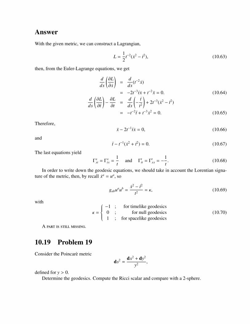
AnswerWith the given metric, we can construct a Lagrangian,

L =12

t−2(x2 − t2), (10.63)

then, from the Euler-Lagrange equations, we get

dds

(∂L∂x

)=

dds

(t−2 x)

= −2t−3t x + t−2 x = 0. (10.64)dds

(∂L∂t

)−∂L∂t=

dds

(−

tt2

)+ 2t−3(x2 − t2)

= −t−2t + t−3 x2 = 0. (10.65)

Therefore,x − 2t−1t x = 0, (10.66)

andt − t−1(x2 + t2) = 0. (10.67)

The last equations yield

Γxxt = Γ

xtx =

1t

and Γttt = Γ

txx = −

1t. (10.68)

In order to write down the geodesic equations, we should take in account the Lorentian signa-ture of the metric, then, by recall xa = ua, so

gabuaub =x2 − t2

t2 = κ, (10.69)

with

κ =

−1 ; for timelike geodesics0 ; for null geodesics1 ; for spacelike geodesics

(10.70)

A .

10.19 Problem 19Consider the Poincarè metric

ds2 =dx2 + dy2

y2 ,

defined for y > 0.Determine the geodesics. Compute the Ricci scalar and compare with a 2-sphere.

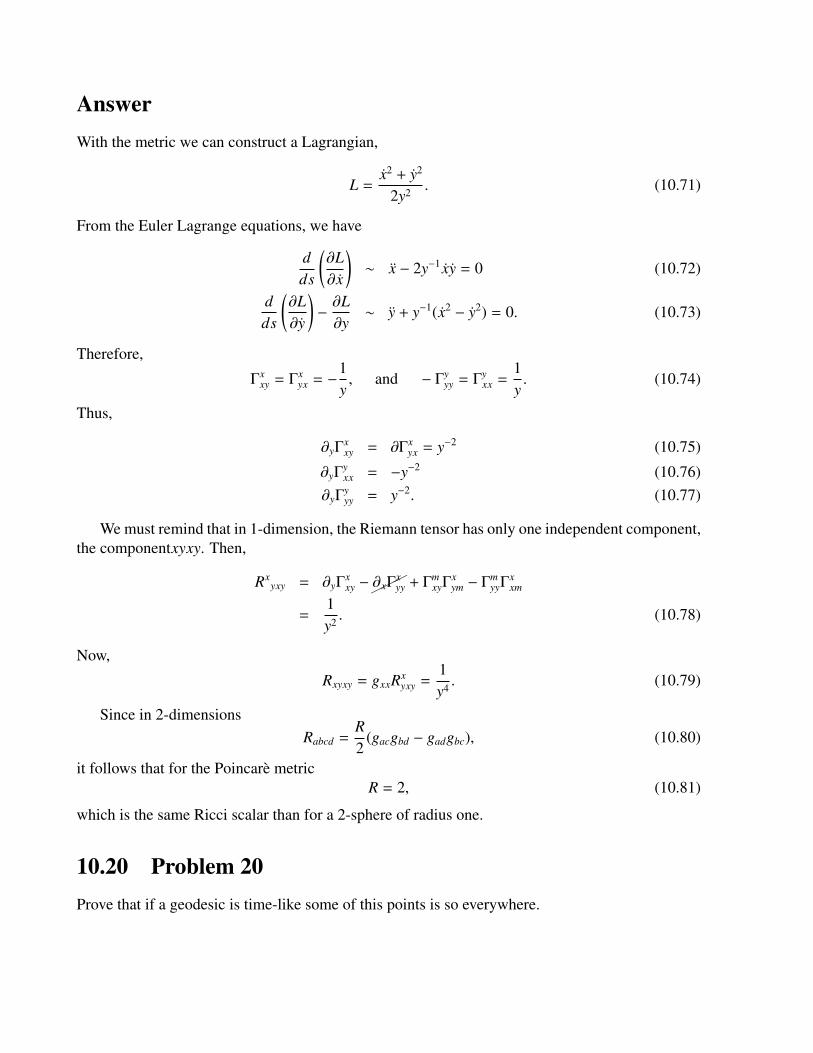
AnswerWith the metric we can construct a Lagrangian,

L =x2 + y2

2y2 . (10.71)

From the Euler Lagrange equations, we have

dds

(∂L∂x

)∼ x − 2y−1 xy = 0 (10.72)

dds

(∂L∂y

)−∂L∂y

∼ y + y−1(x2 − y2) = 0. (10.73)

Therefore,

Γxxy = Γ

xyx = −

1y, and − Γy

yy = Γyxx =

1y. (10.74)

Thus,

∂yΓxxy = ∂Γx

yx = y−2 (10.75)

∂yΓyxx = −y−2 (10.76)

∂yΓyyy = y−2. (10.77)

We must remind that in 1-dimension, the Riemann tensor has only one independent component,the componentxyxy. Then,

Rxyxy = ∂yΓ

xxy −∂xΓ

xyy + Γ

mxyΓ

xym − Γ

myyΓ

xxm

=1y2 . (10.78)

Now,

Rxyxy = gxxRxyxy =

1y4 . (10.79)

Since in 2-dimensionsRabcd =

R2

(gacgbd − gadgbc), (10.80)

it follows that for the Poincarè metricR = 2, (10.81)

which is the same Ricci scalar than for a 2-sphere of radius one.

10.20 Problem 20Prove that if a geodesic is time-like some of this points is so everywhere.

Answer

Note in equation (10.69) that the LHS in fact depend on the point, but in not the case for the RHD.Thus if in a point the geodesic is time-like, it’ll be so in any other point. Same for light-like ortime-like.

10.21 Problem 21A Killing vector satisfy ξa;b + ξb;a = 0. Show that is possible to construct conserved quantities byconsidering objects uaξa, with ua the 4-velocity of the particle.

Answer

A quantity is said to be conserved if its derivative vanish, so, we must expect that

∇b(uaξa) = 0. (10.82)

Then,∇b(uaξa) = (∇bua)ξa + ua(∇bξa). (10.83)

By the Killing vector equation, it follows that the bracket in the last term is antisymmetric underchange a↔ b, so if we contract the whole expression with ub, we get

ub∇b(uaξa) = (ub∇bua)ξa + ubua(∇bξa) = 0, (10.84)

the latter term vanish because of the symmetries, and the former because of the geodesic equationof the particle.

10.22 Problem 22What is the Riemann for a 1-dimensional manifold? Express the Riemann and Ricci tensors interm of the metric for the 2- and 3-dimensional case.

Answer

Because of the symmetries of the Riemann tensor, it’s identically zero for a 1-dimensional mani-fold. In fact, any 1-dimensional manifold is diffeomorphic to R1 or S 1 depending if it’s compact ornot.

A PART IS STILL MISSING.

10.23 Problem 6.10Show that ∇c∇dXa

b − ∇d∇cXab = Ra

ecdXeb + Re

bcdXae .

AnswerLet’s compute the first term.

∇c∇dXab = ∇c(∂dXa

b + ΓadmXm

b − ΓmdbXa

m)= ∂c∂dXa

b − Γmcd∂mXa

b + Γacm∂dXm

b − Γmcb∂dXa

m

+∂c(ΓadmXm

b ) − ΓncdΓ

anmXm

b + ΓacnΓ

ndmXm

b − ΓncbΓ

admXm

n

−∂c(ΓmdbXa

m) + ΓncdΓ

mnbXa

m − ΓacnΓ

mdbXn

m + ΓncbΓ

mdnXa

n . (10.85)

Since the second term is interchanging c↔ d, thus

[∇c,∇d]Xab = −T m

cd(∂mXab − Γ

nmbXa

n + ΓamnXn

b)+Xm

b (∂cΓadm − ∂dΓ

acm + Γ

acnΓ

ndm − Γ

adnΓ

ncm)

−Xam(∂cΓ

mdb − ∂dΓ

mcb + Γ

mcnΓ

ndb − Γ

mdnΓ

ncb)

= −T mcd∇mXa

b + RamcdXm

b + RmbcdXa

m. (10.86)

10.24 Problem 6.11Show that

∇X(∇YZa) − ∇Y(∇XZa) − ∇[X,Y]Za = RabcdZbXcYd. (10.87)

AnswerSince R(X,Y,Z) = ∇X(∇YZ) − ∇Y(∇XZ) − ∇[X,Y]Z is a tensor, it satisfy that

R(X,Y,Z) = XaYbZcR(ea, eb)ec. (10.88)

Moreover, ⟨dxd,R(ea, eb)ec

⟩=

⟨dxd, [∇ea ,∇eb]ec

⟩= ∂aΓ

dbc − ∂bΓ

dac + Γ

damΓ

mbc − Γ

dbmΓ

mac

= Rdcab. (10.89)

Thus,∇X(∇YZd) − ∇Y(∇XZd) − ∇[X,Y]Zd = Rd

cabZcXaYb. (10.90)

10.25 Problem 6.14The line elements or R3 in cartesian, cylindrical and spherical coordinates are given respectivelyby

• ds2(1) = dx2 + dy2 + dz2.

• ds2(2) = dr2 + r2dθ2 + dz2.

• ds2(3) = dr2 + r2dθ2 + r2 sin2 θdφ2.

Find gab, gab and g.

AnswerSince ds2 = gabdxadxb, it follows that,

g(1)ab =

1 0 00 1 00 0 1

(10.91)

g(2)ab =

1 0 00 r2 00 0 1

(10.92)

g(3)ab =

1 0 00 r2 00 0 r2 sin2 θ

(10.93)

gab(1) =

1 0 00 1 00 0 1

(10.94)

gab(2) =

1 0 00 r−2 00 0 1

(10.95)

gab(3) =

1 0 00 r−2 00 0 r−2 sin−2 θ

(10.96)

g(1) = 1 (10.97)g(2) = r2 (10.98)g(3) = r4 sin2 θ. (10.99)

10.26 Problem 6.17Find the geodesic equation for R3 in cylindrical coordinates.

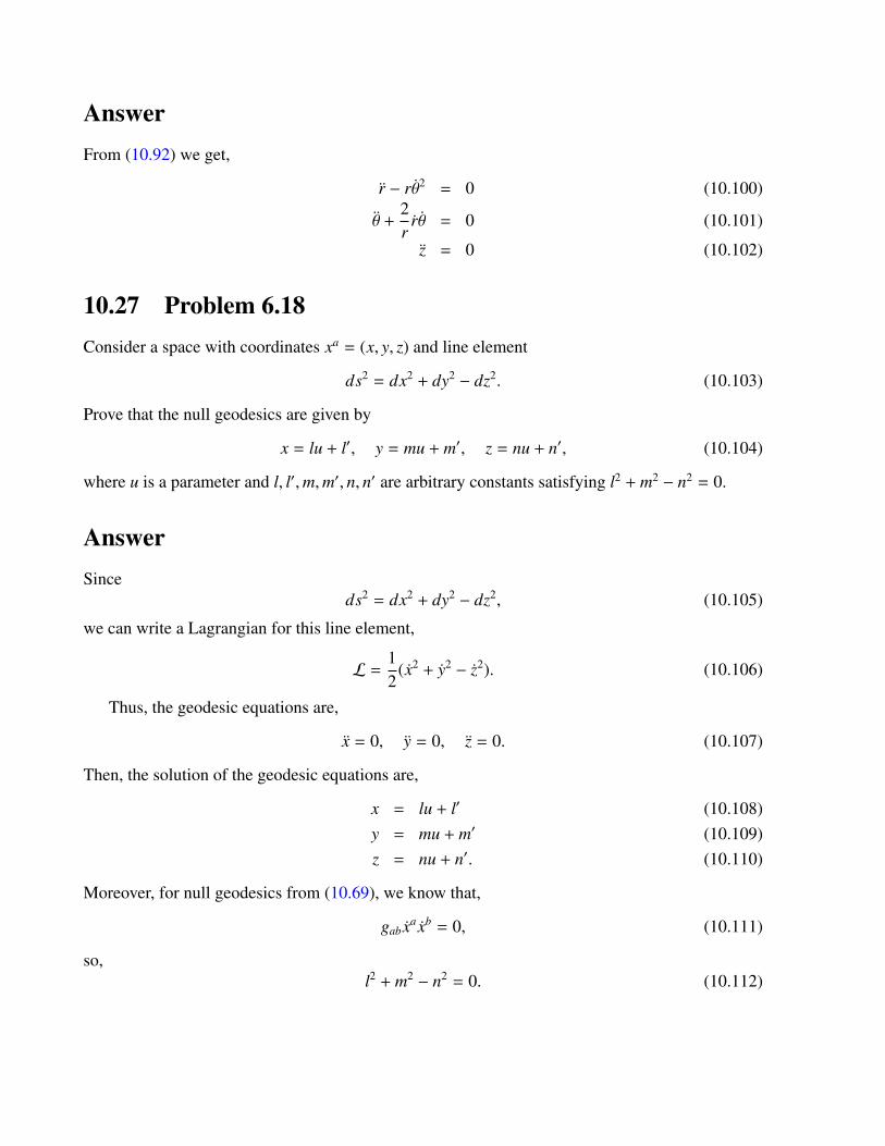
AnswerFrom (10.92) we get,

r − rθ2 = 0 (10.100)

θ +2r

rθ = 0 (10.101)

z = 0 (10.102)

10.27 Problem 6.18Consider a space with coordinates xa = (x, y, z) and line element

ds2 = dx2 + dy2 − dz2. (10.103)

Prove that the null geodesics are given by

x = lu + l′, y = mu + m′, z = nu + n′, (10.104)

where u is a parameter and l, l′,m,m′, n, n′ are arbitrary constants satisfying l2 + m2 − n2 = 0.

AnswerSince

ds2 = dx2 + dy2 − dz2, (10.105)

we can write a Lagrangian for this line element,

L =12

(x2 + y2 − z2). (10.106)

Thus, the geodesic equations are,

x = 0, y = 0, z = 0. (10.107)

Then, the solution of the geodesic equations are,

x = lu + l′ (10.108)y = mu + m′ (10.109)z = nu + n′. (10.110)

Moreover, for null geodesics from (10.69), we know that,

gab xa xb = 0, (10.111)

so,l2 + m2 − n2 = 0. (10.112)

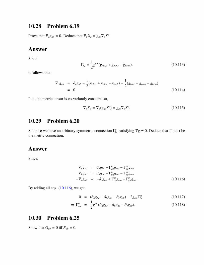
10.28 Problem 6.19Prove that ∇cgab = 0. Deduce that ∇bXa = gac∇bXc.

AnswerSince

Γabc =

12

gam(gmc,b + gmb,c − gbc,m), (10.113)

it follows that,

∇cgab = ∂cgab −12

(gcb,a + gab,c − gac,b) −12

(gba,c + gca,b − gbc,a)

= 0. (10.114)

I. e., the metric tensor is co-variantly constant, so,

∇bXa = ∇b(gacXc) = gac∇bXc. (10.115)

10.29 Problem 6.20Suppose we have an arbitrary symmetric connection Γa

bc satisfying ∇g = 0. Deduce that Γ must bethe metric connection.

AnswerSince,

∇agbc = ∂agbc − Γmabgmc − Γ

macgbm

∇bgac = ∂bgac − Γmbagmc − Γ

mbcgam

−∇cgab = −∂cgab + Γmcagma + Γ

mcbgam. (10.116)

By adding all eqs. (10.116), we get,

0 = (∂agbc + ∂bgac − ∂cgab) − 2gcmΓmbc (10.117)

⇒ Γmab =

12

gmc(∂agbc + ∂bgac − ∂cgab). (10.118)

10.30 Problem 6.25Show that Gab = 0 iff Rab = 0.

AnswerObviously, if Rab = 0 then Gab = 0. Therefore, let’s show the other way.

SinceGab = Rab −

12

gabR, (10.119)

we have that for a , b, Gab = 0⇒ Rab = 0. Moreover, if a = b, the trace of G yields

R =n2

R, (10.120)

but for n , 2, (10.120) doesn’t hold, therefore,

Gab = 0 iff Rab = 0. (10.121)

Part V

Quantum Field Theory

163

Chapter 11QFT I 6

11.1 Problem 1Consider the massless K.G. action,

S =12

∫d4xηµν∂µφ∂νφ, (11.1)

and the dilatation transformation,

xµ → x′µ = Eαxµ, (11.2)φ(x) → φ′(x′) = e−dφαφ(x). (11.3)

1. Show that this transformation is a global symmetry for an appropiate choice of the parametredφ. Find the conserved current associated to this symmery, and verify it’s conserved when φis a classical solution.

2. Show that if there is a mass term then dilatations are no mero a symmetry. Show also that incontrast, a term V(φ) = λφ4 doesn’t spoil the symmetry. What should be the dimension ofthe coupling constant λ?

AnswerLet us find the apropiate value of the constant dφ. In order for dilatations being a symmetry, s = s′.Then

S → S ′ =12

∫d4xe4αηµνe(2−2dφ)α∂µφ∂νφ

=12

∫d4xηµνe(2−2dφ)α∂µφ∂νφ

= S if dφ = 1. (11.4)

165

Thus,φ(x)→ φ′(x′) = e−αφ(x). (11.5)

Now, if we restrict ourselves to infinitesimal transformations, we can find the Nöther conservedcurrent by using the formulae derived in class,

jµa =∂L

∂(∂µφi)[A ν

a ∂νφi −Fi,a]−A µ

a L

= AaνΘµν −

∂L

∂(∂µφi)Fi,a. (11.6)

Then, for our particular sut up, we have,

δxµ = αxµ = εaA µa , (11.7)

δφ = −αφ = εaFi,a, (11.8)∂L

∂(∂µφ)= ∂µφ. (11.9)

In the above equations, i = φ, a = 1, ε = α, A µ = xµ and Fi,a = −φ.On the other hand, for the massless KG theory,

Θµν = ∂µφ∂νφ −12ηµν∂αφ∂αφ. (11.10)

=⇒ ∂µΘµν = ∂νφφ + ∂µφ∂µ∂

νφ − ηµν∂µ∂αφ∂αφ

= ∂νφφ + ∂µφ∂µ∂νφ − ∂ν∂αφ∂αφ

= ∂νφφ

= 0. (11.11)

In the last line we have used the eqs. of motion.From (11.10), we calculate the trace,

Θµµ = ∂µφ∂µφ − 2∂µφ∂µφ = −∂µφ∂µφ. (11.12)

Thus,

∂µ jµ = Θµµ +Aν∂µΘµν − ∂µ

(∂L

∂(∂µφ)F

)= −∂µφ∂µφ + ∂µ(φ∂µφ)= φφ

= 0. (11.13)

.

We saw that the massless KG equation is indeed dilatation invariant. If we add a mass term or aλφ4 potential, those do not affect the invariance of the kinetic term, so we can verify its invariance(or not) individually. Then,

S m → S m′12

∫d4xe4αm2φ2e−2α , S . (11.14)

S λ → S λ′ = λ

∫d4xe4αφ4e−4α = S λ. (11.15)

Thus, the mass term spoils the dilatation symmetry whilst the quartic potential on phi doesn’t.Additionally, the λ must be adimensional, so that the φ4 match the dimensions of the volume form.

11.2 Problem 2

Consider th elagrangian of QED, for massless fermions, and the dilatation transformation,

xµ → eαxµ (11.16)Aµ → e−dAαAµ (11.17)ψ → e−dψαψ. (11.18)

1. Find the values of dA and dψ in order for dilatations being a symmetry.

2. Calculate the conserved current for this symmetry and express it in terms os the energy-momentum tensor of the theory. Verify that that its conservation is a consecuence of the factthat the energy-momentum is traceless in the massless theory.

3. Include the mass term for fermions in the lagrangian. Compute the new Nöther corrent andverify it’s not conserved, relate its divergence with the trace of the energy-momentum tensor.

Answer

As we’ve discussed in the above problem, we can check the dilatation invariace term by term. Sincethe lagrangian of QED is

LQED = ıψ(/∂ − m)ψ −14

F2 − qψγµAµψ, (11.19)

let’s check first the EM lagrangian.

Each term of this lagrangian contents a couple of derivatis and a couple of A’s, therefore,

S EM → S ′EM = −

∫d4x e4α1

4F2e−2−2dA

= S if dA = 1. (11.20)

S D → S ′D =

∫d4xe4αψγµ∂µψe−α−2α

= S if dψ =32. (11.21)

S I → S ′I = −

∫e4αqφγµAµφe−4α = S I . (11.22)

Then, the right values of the parameters are,

dA = 1 and dψ =32. (11.23)

Let’s calculate the energy-momentum tensor using,

Θµν =∂L

∂(∂µφi)∂νφi − η

µνL . (11.24)

Then,Θµν = ıψ∂µγνψ − Fµλ∂νAλ − ηµνLQED. (11.25)

And, for infinitesimal transformation, we have,

δxµ = αxµ, (11.26)δAµ = −αAµ, (11.27)

δψ = −32αφ. (11.28)

Following the usual method, the conserved current must be,

jµ =∂L

∂(∂µφi)[A ν∂νφi −Fi

]−A µL (11.29)

=∂L

∂(∂µφi)[Aν∂

νφi −Fi]−Aνη

µνL (11.30)

= −∂L

∂(∂µφi)Fi +AνΘ

µν (11.31)

11.3 Problem 3Consider the Dirac lagrangians

L = ψ(ı/∂ − m)ψ (11.32)

and

L ′ = ψ(ı

2γµ←→∂ µ − m

)ψ. (11.33)

Verify that they are classically equivalents. Compute the energy-momentum tensor to showthey’re different, but their conserved charges are the same.

Answer

Consider the prime action,

S ′ =∫

d4xψ(ı

2γµ←→∂ µ − m

)ψ

=

∫d4x

(ı

2ψγµ∂µψ −

ı

2∂µψγ

µψ − mψψ)

=

∫d4x

(ıψγµ∂µψ −

ı

2∂µ(ψγµψ) − mψψ

)=

∫d4x

(ıψγµ∂µψ − mψψ

)= S . (11.34)

We have made use of the fact that φ→ 0 as long as |x| → ∞Hence, classically both lagrangians are equivalent.Now, let’s calculate their energy-momentum tensors. Since,

Θµν =∂L

∂(∂µφi)∂νφi − η

µνL , (11.35)

then,

Θµν1 = ıψγµ∂νψ − ηµν

(ψ(ı/∂ − m)ψ

),

= ıψγµ∂νψ (11.36)

Θµν2 =

ı

2(ψγµ∂νψ − ∂νψγµψ

)− ηµνψ

(ı

2γµ←→∂ µ − m

)ψ

=ı

2(ψγµ∂νψ − ∂νψγµψ

). (11.37)

We have used the equations of motion for both lagrangians,

(ı/∂ − m)ψ = 0; ı∂µψγµ + mψ = 0, (11.38)

That’s nothing but evaluate φ→ φcl.

The conserved currents are,

Pµ1 = ı

∫d3x ψγ0∂µψ. (11.39)

Pµ2 =

∫d3x

ı

2

(ψγ0∂µψ − ∂µψγ0ψ

)= ı

∫d3x ψγ0∂µψ + (B.T.) (11.40)

Thus, the conserved charges are the same, as we expected.

Chapter 12QFT I 7

12.1 Problem 1• Show that the conserved U(1)-charge in the quantum theory of a free complex scalar,

QU(1) = ı

∫d3x : φ†

←→∂ 0φ :, (12.1)

is given by

QU(1) =

∫dp

(2π)3

(a†pap − b†pbp

). (12.2)

• Has the state a†pb†q |0〉 a defined charge?

• Calculate the commutator [QU(1),H], where H is the Hamiltonian of the theory.

AnswerWe already know that the modes expansion of the complex scalar field is

φ(x) =∫

d3 p(2π)3

1√2Ep

ape−ıp·x + b†peıp·x

∣∣∣∣∣∣∣p0=Ep

(12.3)

and

φ†(x) =∫

d3 p(2π)3

1√2Ep

bpe−ıp·x + a†peıp·x

∣∣∣∣∣∣∣p0=Ep

. (12.4)

Then,

∂0φ(x) = −ı∫

d3 p(2π)3

√Ep

2

ape−ıp·x − b†peıp·x

∣∣∣∣∣∣∣p0=Ep

, (12.5)

171

and

φ(x) = −ı∫

d3 p(2π)3

√Ep

2

bpe−ıp·x − a†peıp·x

∣∣∣∣∣∣∣p0=Ep

. (12.6)

Thus

QU(1) = ı

∫d3x : φ†∂0φ − (∂0φ

†)φ :

= :∫

d3x∫

d3 p(2π)3

d3q(2π)3

12

√Eq

Ep

[bpe−ıp·x + a†peıp·x

aqe−ıq·x − b†qeıq·x

−

bqe−ıq·x − a†qeıq·x

ape−ıp·x + b†peıp·x

]:

=

∫d3 p

(2π)3

d3q(2π)3

12

(2π)3δ3(p − q)

eı(Ep−Eq)t

√Eq

Ep:−bpb†q + a†paq − bqb†p + a†qap

:

=

∫d3 p

(2π)3 (a†pap − b†pbp). (12.7)

Let us now calculate the charge of the state a†pb†q |0〉. Then,

QU(1)a†pb†q |0〉 =∫

d3k(2π)3 (a†kak − b†kbk)a†pb†q |0〉

= a†pb†q |0〉 − a†pb†q |0〉

= 0a†pb†q |0〉 , (12.8)

therefore, this state has no charge, as it was expected so that each creator operator contribute withopposite charge.

On the other hand,

[QU(1),H] =∫

d3 p(2π)3

d3 p′

2π)3 Ep′[a†pap − b†pbp, a

†

p′ap′ + b†p′bp′]

=

∫d3 p

(2π)3

d3 p′

2π)3 Ep′[

a†pap, a†

p′ap′]−

[b†pbp, b

†

p′bp′]

=

∫d3 p

(2π)3

d3 p′

2π)3 Ep′a†p

[ap, a

†

p′

]ap′ + a†p′

[a†p, ap′

]ap

−b†p[bp, b

†

p′

]bp′ − b†p′

[b†p, bp′

]bp

= 0. (12.9)

12.2 Problem 2

In the quantum theory for a free Dirac field, consider the modes expansion

ψ(x) =∫

d3 p(2π)3

1√2Ep

∑s=1,2

(ap,sus(p)e−ıp·x + b†p,svs(p)eıp·x

)∣∣∣∣∣∣∣p0=Ep

. (12.10)

Suppose that the spinors u and v are normalized like

us(p)us′(p) = Nuδss′ , vs(p)vs′(p) = −Nvδss′ , (12.11)

with Nu and Nv are positive factors (possibly depending on p)

• Find the expression for the creation and annihilation operators in term of the field operatorsψ and ψ.

• Compute the whole set of anti-commutator of the creator and annihilator operators.

• How must the normalization constant of spinors be chosen in order to satisfy the relations

ap,s, a†

p′,s′ = bp,s, b†

p′,s′ = (2π)3δ(3)(p − p′)δss′? (12.12)

Answer

Hence,

ψ(x) =∫

d3 p(2π)3

1√2Ep

∑s=1,2

(ap,sus(p)e−ıp·x + b†p,svs(p)eıp·x

)∣∣∣∣∣∣∣p0=Ep

, (12.13)

it follows that

ψ(x) =∫

d3 p(2π)3

1√2Ep

∑s=1,2

(bp,svs(p)e−ıp·x + a†p,sus(p)eıp·x

)∣∣∣∣∣∣∣p0=Ep

. (12.14)

Now, we can take the Fourier transform of ψ and ψ,∫d3xeı~k·~xψ(x) =

1√

2Ek

∑s=1,2

(ak,sus(k)e−ıEkt + b†

−k,svs(−k)eıEkt)

(12.15)∫d3xeı~k·~xψ(x) =

1√

2Ek

∑s=1,2

(bk,svs(k)e−ıEkt + a†

−k,sus(−k)eıEkt). (12.16)

By using the normalization conditions, we get,

ak,s =

√2Ek

Nu

∫d3x eık·xus(k)ψ(x) (12.17)

a†k,s =√

2Ek

Nu

∫d3x e−ık·xus(k)ψ(x) (12.18)

bk,s = −

√2Ek

Nv

∫d3x eık·xvs(k)ψ(x) (12.19)

ak,s = −

√2Ek

Nv

∫d3x e−ık·xvs(k)ψ(x). (12.20)

As we can to calculate their anti-commutator relations, we should remind thatψ(t, ~x), ψ(t, ~y)

= δ(3)(x − y), (12.21)

and whatever other anti-commutator vanish.So,

ak,s, ak′,s′= 0 (12.22)

a†k,s, a†

k′,s′

= 0 (12.23)

bk,s, bk′,s′= 0 (12.24)

b†k,s, b†

k′,s′

= 0 (12.25)

ak,s, b†

k′,s′

= 0 (12.26)

bk,s, a†

k′,s′

= 0. (12.27)

Additionally, we know thatus(p)vs′(p) = vs(p)us′(p) = 0. (12.28)

Then, ak,s, bk′,s′

= 0 (12.29)

a†k,s, b†

k′,s′

= 0. (12.30)

Finally, ak,s, a

†

k′,s′

=

2√

EE′

N2u

∫d3xd3yus(k)us′(k′)eı(k·x−k′·y) ψ(t, x)ψ(t, y)

=

2√

EE′

N2u

us(k)us′(k′)∫

d3xeı(k−k′)·x

= (2π)3 2√

EE′

N2u

us(k)us′(k′)δ(3)(k − k′)

= (2π)3 2ENuδss′δ

(3)(k − k′), (12.31)

and bk,s, b

†

k′,s′

=

2√

EE′

N2v

∫d3xd3yvs(k)vs′(k′)eı(k·x−k′·y) ψ(t, x)ψ(t, y)

=

2√

EE′

N2v

vs(k)vs′(k′)∫

d3xeı(k−k′)·x

= (2π)3 2√

EE′

N2v

vs(k)vs′(k′)δ(3)(k − k′)

= −(2π)3 2ENuδss′δ

(3)(k − k′). (12.32)

12.3 Problem 3Show that the quantity Epδ

(3)(p−q) is Lorentz invariant, therefore the 1-particle states (2Ep)1/2a†p |0〉have an Lorentz invariant normalization.

AnswerFirst, we note that the rotacional part of the Lorentz group keeps the quantity, we are interestedon, invariant, so that the energy remains the same and the determinante of a rotation matrix (for aproper rotation) is 1. Therefore, we can consentrate just on the boost transformation.

Actually, we know how a delta function transform

δ( f (x) − f (x0)) =∑

i

1| f ′(xi)|

δ(x − xi), (12.33)

with xi are the zeroes of the funtion f .Without loss of generality, we can onsider a boost in the x direction, s.t. p′ = p′x = γ(p + βE)

and E′ = γ(E + βp). Then,

Eδ(3)(p − q) = Eδ(3)(p′ − q′)dp′

dp

= Eδ(3)(p′ − q′)γ(1 + β

dEdp

)= Eδ(3)(p′ − q′)

γ

E(E + βp)

= Eδ(3)(p′ − q′)E′

E= E′δ(3)(p′ − q′). (12.34)

Thus, the quantity Eδ(3)(p − q) in Lorentz invariant.

Furthermore, for a one-particle state,(2Ep)1/2a†p |0〉, we have⟨0∣∣∣(2Eq)1/2aq(2Ep)1/2a†p

∣∣∣ 0⟩ = 2Ep(2π)3δ(3)(p − q), (12.35)

which we have proved to be Lorentz invariant.

12.4 Problem 4

For the electromagnetic field quantized in the radiation gauge, show that

•

[Ai(t, ~x), E j(t, ~y)] = −ı∫

d3k(2π)3 eı~k·(~x−~y)

δi j −kik j

|~k|2

.•

H =∫

d3k(2π)3

∑λ=1,2

ωka†

k,λak,λ,

and

~P =∫

d3k(2π)3

∑λ=1,2

~ka†k,λak,λ.

•

S i j = ı

∫d3k

(2π)3

∑λ,λ′

[ε iλ′(k)ε j∗

λ − εi∗λ (k)ε j

λ′

]a†k,λak,λ′ .

Answer

The modes expansion of the vector potential is

Ai(x) =∫

d3k(2π)3

1√

2ωk

∑λ=1,2

ε iλ(k)ak,λe−ık·x + ε i∗

λ (k)a†k,λeık·x

∣∣∣∣∣∣∣k0=ωk

. (12.36)

Then,

Ei(x) = ı∫

d3k(2π)3

√ωk

2

∑λ=1,2

ε iλ(k)ak,λe−ık·x − ε i∗

λ (k)a†k,λeık·x

∣∣∣∣∣∣∣k0=ωk

. (12.37)

From these equations, it follows that,

[Ai(t, ~x), E j(t, ~y)] = ı

∫d3k

(2π)3

d3q(2π)3

12

√ωq

ωk∑λ,λ′

−ε i

λ(k)ε j∗λ′ (q)[ak,λ, a

†

q,λ′]e−ı(ωk−ωq)teı(~k·~x−~q·~y)

+ε i∗λ (k)ε j

λ′(q)[a†k,λ, aq,λ′]eı(ωk−ωq)te−ı(~k·~x−~q·~y)

= −ı

∫d3k

(2π)3

12

∑λ

ε iλ(k)ε j∗

λ′ (k) + ε i∗λ (−k)ε j

λ′(−k)

eı~k·(~x−~y)

= −ı

∫d3k

(2π)3 eı~k·(~x−~y)

δi j −kik j

|~k|2

= −ıδ

i jtr(~x − ~y) (12.38)

Now, we shall compute the quantum Hamiltonian of the system,

H =12

∫d3x : E2 + B2 : . (12.39)

Since~E(x) = ı

∫d3k

(2π)3

√ω

2

∑λ

~ελ(k)ak,λe−ık·x − ~ε∗λ(k)a†k,λe

ık·x, (12.40)

and~B(x) = ı

∫d3k

(2π)3

1√

2ω

∑λ

~k × ~ελ(k)ak,λe−ık·x − ~k × ~ε∗λ(k)a†k,λe

ık·x, (12.41)

it follows that

: E2 : = − :12

∫d3k

(2π)3

d3k′

(2π)3

√ωω′

∑λ,λ′


ık·x

~ελ′(k′)ak′,λ′e−ık

′·x − ~ε∗λ′(k′)a†k′,λ′e

ık′·x

:

= −12

∫d3k

(2π)3

d3k′

(2π)3

√ωω′

∑λ,λ′

~ελ(k) · ~ελ′(k′)ak,λak′,λ′e−ı(k+k′)·x

−~ελ(k) · ~ε∗λ′(k′)a†k′,λ′ak,λe−ı(k−k′)·x − ~ε∗λ(k) · ~ελ′(k′)a

†

k,λak′,λ′eı(k−k′)·x

+~ε∗λ(k) · ~ε∗λ′(k′)a†k,λa

†

k′,λ′eı(k+k′)·x

, (12.42)

so, ∫d3x : E2 : = −

12

∫d3k

(2π)3 |~k|

∑λ,λ′

~ελ(k) · ~ελ′(−k)ak,λa−k,λ′e−2ıωt

−~ελ(k) · ~ε∗λ′(k)a†k,λ′ak,λ − ~ε∗λ(k) · ~ελ′(k)a†k,λak,λ′

+~ε∗λ(k) · ~ε∗λ′(−k)a†k,λa†

−k,λ′e2ıωt

. (12.43)

And

: B2 : = −12

∫d3k

(2π)3

d3k′

(2π)3

1√ωω′

∑λ,λ′

:~k × ~ελ(k)ak,λe−ık·x − ~k × ~ε∗λ(k)a†k,λe

ık·x

~k′ × ~ελ′(k′)ak′,λ′e−ık

′·x − ~k′ × ~ε∗λ′(k′)a†k′,λ′e

ık′·x

:

= −12

∫d3k

(2π)3

d3k′

(2π)3

1√ωω′

∑λ,λ′

(~k × ~ελ(k)) · (~k′ × ~ελ′(k′))ak,λak′,λ′e−ı(k+k′)·x

−(~k × ~ελ(k)) · (~k′ × ~ε∗λ′(k′))a†k′,λ′ak,λe−ı(k−k′)·x

−(~k × ~ε∗λ(k)) · (~k′ × ~ελ′(k′))a†


+(~k × ~ε∗λ(k)) · (~k′ × ~ε∗λ′(k′))a†k,λa

†


, (12.44)

so that

∫d3x : B2 : = −

12

∫d3k

(2π)3

1

|~k|

∑λ,λ′

(~k × ~ελ(k)) · ( ~−k × ~ελ′(−k))ak,λa−k,λ′e−2ıωt

−(~k × ~ελ(k)) · (~k × ~ε∗λ′(k))a†k,λ′ak,λ

−(~k × ~ε∗λ(k)) · (~k × ~ελ′(k))a†k,λak,λ′

+(~k × ~ε∗λ(k)) · ( ~−k × ~ε∗λ′(−k))a†k,λa†

−k,λ′e2ıωt

. (12.45)

Now, we shall use the vectorial identity

(~k × ~ε) · (~k × ~ε′) = |~k|2~ε · ~ε′ − (~k · ~ε)(~k · ~ε′), (12.46)

and the polarization conditions

~k · ~ε = ~k · ~ε′ = 0, (12.47)

we get finally,

H = −14

∫d3k

(2π)3 |~k|

∑λ,λ′

~ελ(k) · ~ελ′(−k)ak,λa−k,λ′e−2ıωt

−~ελ(k) · ~ε∗λ′(k)a†k,λ′ak,λ − ~ε∗λ(k) · ~ελ′(k)a†k,λak,λ′

+~ε∗λ(k) · ~ε∗λ′(−k)a†k,λa†

−k,λ′e2ıωt

−

14

∫d3k

(2π)3 |~k|

∑λ,λ′

−~ελ(k) · ~ελ′(−k)ak,λa−k,λ′e−2ıωt

−~ελ(k) · ~ε∗λ′(k)a†k,λ′ak,λ

−~ε∗λ(k) · ~ελ′(k)a†k,λak,λ′

−~ε∗λ(k) · ~ε∗λ′(−k)a†k,λa†

−k,λ′e2ıωt

=

∫d3k

(2π)3 |~k|

∑λ,λ′

12

(~ελ(k) · ~ε∗λ′(k) + ~ε∗λ′(k) · ~ελ(k)

)a†k,λak,λ′

=

∫d3k

(2π)3 |~k|

∑λ

a†k,λak,λ. (12.48)

We have use12

(~ελ(k) · ~ε∗λ′(k) + ~ε∗λ′(k) · ~ελ(k)

)= δλ,λ′ . (12.49)

Also, in the same way,

~P =

∫d3x : ~E × ~B :

= −

∫d3x

d3k(2π)3

d3k′

(2π)3

12

1√

EE′

∑λλ′


ık·x

×~k′ × ~ελ′(k′)ak′,λ′e−ık

′·x − ~k′ × ~ε∗λ′(k′)a†k′,λ′e

ık′·x

= −

∫d3x

d3k(2π)3

d3k′

(2π)3

12

1√

EE′

∑λλ′

~ελ(k) × ~k′ × ~ελ′(k′)ak,λak′,λ′e−ı(k+k′)·x

−~ελ(k) × ~k′ × ~ε∗λ′(k′)a†k′,λ′ak,λe−ı(k−k′)·x − ~ε∗λ(k) × ~k′ × ~ελ′(k′)a

†


+~ε∗λ(k) × ~k′ × ~ε∗λ′(k′)a†k,λa

†


=

∫d3k

(2π)3

∑λλ′

12

~k(~ελ(k) · ~ελ′(−k))ak,λa−k,λ′e−2ıωt

+~k(~ελ(k) · ~ε∗λ′(k))a†k,λ′ak,λ + ~k(~ε∗λ(k) · ~ελ′(k))a†k,λak,λ′

~k(~ε∗λ(k) · ~ε∗λ′(−k))a†−k,λ′ak,λe2ıωt

=

∫d3k

(2π)3

∑λ

~ka†k,λak,λ, (12.50)

where we’ve used (12.49) and~ελ(k) · ~ε(∗)

λ′ (−k) = 0. (12.51)

Finally, from (12.36) and (12.37), we get

S i j = −

∫d3x

d3k(2π)3

d3k′

(2π)3

12

√ω′

ω

∑λλ′(

ε iλ(k)ε j

λ′(k′) − ε j

λ(k)ε iλ′(k

′))

ak,λak′,λ′e−ı(k+k′)·x

−(ε iλ(k)ε∗ j

λ′ (k′) − ε j

λ(k)ε∗iλ′(k′))

a†k′,λ′ak,λe−ı(k−k′)·x

+(ε∗iλ (k)ε j

λ′(k′) − ε∗ j

λ (k)ε iλ′(k

′))

a†k,λak′,λ′eı(k−k′)·x

−(ε∗iλ (k)ε∗ j

λ′ (k′) − ε∗ j

λ (k)ε∗iλ′(k′))

a†k,λa†


= −

∫d3k

(2π)3

12

∑λ,λ′

2ε

jλ(k)ε∗iλ′(k) − ε i

λ(k)ε∗ jλ′ (k)

a†k,λak,λ′

= −

∫d3k

(2π)3

∑λ,λ′

ε

jλ(k)ε∗iλ′(k) − ε i

λ(k)ε∗ jλ′ (k)

a†k,λak,λ′ (12.52)

Chapter 13Miscellaneous

13.1 NotationThrough this article we shall use the following notation.

• Minkowski metric: ηµν = diag(+1,−1,−1,−1).

• Pauli matrices:

σ1 =

(0 11 0

)(13.1)

σ2 =

(0 −ıı 0

)(13.2)

σ3 =

(1 00 −1

). (13.3)

The Pauli matrices satisfy the Clifford algebra σi, σ j = 21δi j. Additionally, σµ = (1, σi),and σµ = (1,−σi).

13.2 Gamma matrices in the chiral representationConsider the Gamma matrices in the chiral representation

Γµ =

(0 σµ

σµ 0

). (13.4)

Let’s prove that they satisfy the Clifford algebra.(0 σµ

σµ

),

(0 σν

σν

)=

(σµσν + σνσµ 0

0 σµσν + σνσµ

). (13.5)

Now, let’s consider the cases µ = ν = 0, µ = 0, ν = i and µ = i, ν = j.

181

1. If µ = ν = 0,σ0σ0 + σ0σ0 = 21, (13.6)

andσ0σ0 + σ0σ0 = 21. (13.7)

2. If µ = 0.ν = i, since σi = −σi,

σ0σi + σiσ0 = −σi + σi

= 0, (13.8)

and

σ0σi + σiσ0 = σi − σi

= 0. (13.9)

3. If µ = i, ν = j,

σiσ j + σ jσi = −σi, σ j

= −21, (13.10)

and

σiσ j + σ jσi = −σi, σ j

= −21. (13.11)

Finally, from (13.6), (13.7), (13.10) and (13.11), we can write

σµσν + σνσµ = 2ηµν1 (13.12)σµσν + σνσµ = 2ηµν1, (13.13)

andγµ, γν = 2ηµν1. (13.14)

13.3 Scalars from Weyl spinorsConsider the products ψ†LψR and ψ†RψL. We want to prove that they transform like scalars.

Since, under Lorentz transformations

ψL 7→ ψ′L = ΛLψL = exp((−ı~θ − ~η)

~σ

2

)ψL, (13.15)

ψR 7→ ψ′R = ΛRψR = exp((−ı~θ + ~η)

~σ

2

)ψR, (13.16)

Then

ψ†LφR 7→ ψ′L†ψ′R = (ΛLψL)†ΛRψR

= ψ†L exp((ı~θ − ~η)

~σ

2

)exp

((−ı~θ + ~η)

~σ

2

)ψR

= ψ†LψR. (13.17)

Similarly,

ψ†RφL 7→ ψ′R†ψ′L = (ΛRψR)†ΛLψL

= ψ†R exp((ı~θ + ~η)

~σ

2

)exp

((−ı~θ − ~η)

~σ

2

)ψL

= ψ†RψL. (13.18)

13.4 Determinant of a deformation of the identityConsider a deformation of the identity matrix, let’s say 1 + X, we want to compute

det(1 + X) =?. (13.19)

Actually, we can do more than one trick for calculating this quantity.First, we’ll use the formulae

det(exp(M)) = exp(tr(M)) (13.20)

exp(M) =∞∑

n=0

Mn

n!(13.21)

ln(1 + M) =∞∑

n=1

(−1)n+1 Mn

n. (13.22)

From (13.20), we have

det(1 + X) = exp(tr(ln(1 + X)))

= exp(tr

(X −

X2

2+

X3

3− · · ·

))= 1 + tr(X) −

12

tr(X2) +12

(tr(X))2

+1

12

(4tr(X3) − 3tr(X2)tr(X) + 2(tr(X))3

)+ · · · . (13.23)

Nonetheless, if the components of X 1, we get

det(1 + X) 1 + tr(X). (13.24)

Another way of get the solution is by writing

det(1 + X) = ε i1···in(δ1i1 + X1i1) · · · (δnin Xnin), (13.25)

from this equation we can see that the expansion of above is never infinite, and we obtain a sum of“generalised" cofactors matrices. So,

det(1 + X) = 1 + tr(X) + · · · + det(X). (13.26)

13.5 Lorentz currents for a real scalar fieldIn the class we’ve check that for a Lorentz transformation, a real scalar field has a Nöther conservedcurrent

jµρσ = ∂µφ(δνρxσ − δνσxρ)∂νφ − (δµρxσ − δµσxρ)L , (13.27)

now, we want to write that in term of the energy momentum tensor,

Θµν = ∂µφ∂νφ − ηµνL . (13.28)

Then

jµρσ = ∂µφ(ηνρxσ − ηνσxρ)∂νφ − (ηµρxσ − ηµσxρ)L= ∂µφ(δρνxσ − δσν xρ)∂νφ − (ηµρxσ − ηµσxρ)L= ∂µφ(δρνxσ − δσν xρ)∂νφ − ηµν(δρνxσ − δσν xρ)L= (δρνxσ − δσν xρ)(∂µφ∂νφ − ηµνL )= (δρνxσ − δσν xρ)Θµν

= xσΘµρ − xρΘµσ. (13.29)

13.6 Conservation of the KG inner productLet’s define the Klein-Gordon inner product as

〈φ1|φ2〉 =ı

2

∫d3x φ1

←→∂ φ2. (13.30)

Then

∂0 〈φ1|φ2〉 =ı

2

∫d3x

(∂0φ1∂0φ2 + φ1∂

20φ2 − ∂

20φ1φ2 −

∂0φ1∂0φ2

)=

ı

2

∫d3x

(m2φ1φ2 −m2φ1φ2 + φ1∇

2φ2 − ∇2φ1φ2

)=

ı

2

∫d3x

(∂iφ1∂

iφ2 −∂iφ1∂iφ2 + ∂i(φ1∂

iφ2 − ∂iφ1φ2)

)= 0. (13.31)

Here, we have applied the definition of the right-left derivative and then act with ∂0. After that,using the KG eqs. of motion (remember that both scalars have the same mass) and integrating byparts, we get down to the last line, where we argue that φ→ 0, if |x| → ∞.

We conclude that the Klein-Gordon inner product is constant in time.

13.7 Nöther charge for translationWe already know that the Nöther current for tranlation is the energy momentum tensor, so in orderto compute its associate charge, we fix the first index to 0, i.e.,

Pµ =

∫d3x Θ0µ =

∫d3x (∂0φ∂µ − η0µL . (13.32)

If µ = i, we have

Pi = −ı

2

∫d3x

(∂0φı∂

iφ + ∂0φı∂iφ

)= −

ı

2

∫d3x

(∂0φı∂

iφ − ∂0φı∂iφ

)=

⟨φ|ı∂i|φ

⟩, (13.33)

in the intermiddle step, we’ve dropped the divergence, so that (as usual) we demand phi→ 0, |x| →∞.

For µ = 0,

P0 =

∫d3x

(∂0φ∂0φ −

12

((∂0φ)2 − (∂iφ)2 − m2φ2))

=12

∫d3x

(∂0φ)2 + φ(∂i∂

i + m2)φ)

=ı

2

∫d3x

(φı∂0∂0φ − ∂0φı∂

0φ)

=⟨φ|ı∂0|φ

⟩. (13.34)

Thus,Pµ = 〈φ|ı∂µ|φ〉 . (13.35)

13.8 Spinorial LagrangianConsider the lagrangian for left-handed Weyl spinors,

L = (cte)ψ†Lσµ∂µψL. (13.36)

One would like the lagrangian to be real, so

(cte)ψ†Lσµ∂µψL = (cte)∗ψt

Lσ∗µ∂µψ

∗L

= −(cte)∗ψ†Lσµ∂µψL +(((((((((

Boundary term , (13.37)

Therefore,(cte)∗ = −(cte). (13.38)

Chapter 14Does it need a name?

14.1 Wick’s TheoremBy using the Wick’s theorem, compute:

1.⟨0|T φ4(x)φ4(y)|0

⟩2. T : φ4(x) :: φ4(y) :

3.⟨0|T ψ(x)ψ(x)ψ(y)ψ(y)|0

⟩.

Answera Wick’s theorem tells that one should consider all possible contractions of the fields, for thiscase, there are three possibilities, all x and y contracted with themselves, or with each other andfinally a couple of crossed contractions and a pair of self-contractions.

⟨0|T φ4(x)φ4(y)|0

⟩= 9(D(x − x))2(D(y − y))2

+72(D(x − y))2D(x − x)D(y − y)+24(D(x − y))4. (14.1)

The factors came from

• 3 different ways of contracting four φ(x) or φ(y) among themselves.

• 6 different ways of contracting a pair of φ(x) or φ(y) among themselves, times 2 ways ofcontract the remaining fields but crossed.

• 4! (no question)

187

b Since inside the time-ordering operator there are normal products, one must apply the non-equal-time-contraction Wick’s theorem. So,

T : φ4(x) :: φ4(y) : = : φ4(x)φ4(y) : +16 : φ3(x)φ3(y) : D(x − y)+72 : φ2(x)φ2(y) : (D(x − y))2

+96 : φ(x)φ(y) : (D(x − y))3

+4!(D(x − y))4. (14.2)

The symmetry factors are

• 16 ways of taking a pair from two set of four.

• 72... just like before, or 72 = 4232

2! .

• 96 = 423222

3! .

• 4!.

c Finally

⟨0|T ψ(x)ψ(x)ψ(y)ψ(y)|0

⟩=

⟨0|T ψα(x)ψα(x)ψβ(y)ψβ(y)|0

⟩= S αα(x − x)S ββ(y − y)−S βα(y − x)S αβ(x − y). (14.3)

14.2 2→ 2 Scattering in gφ3

In the theory gψ3 calculate, directly from the Dyson expansion and by using the Wick’s theorem,the first non-trivial contribution to the matrix element of S for a 2→ 2 scattering.

AnswerLet φ be a real scalar field with lagrangian

L =12∂µφ∂

µφ −m2φ2 −

g3!φ3, (14.4)

then,Hint =

g3!

: φ3 : . (14.5)

The Dyson expansion is

S = 1 + (−ı)∫

d4xHI(x) +(−ı)2

2!

∫dxd4yT HI(x)HI(y) + · · · . (14.6)

The 2→ 2 scattering is given by ⟨~p1~p2|S |~k1~k2

⟩, (14.7)

with ~p , ~k. Thus, ⟨~p1~p2|S (0)|~k1~k2

⟩=

⟨~p1~p2|1|~k1~k2

⟩= 0. (14.8)

⟨~p1~p2|S (1)|~k1~k2

⟩= (−ı)2(ı)2

(−ı

g3!

) ∫d3z1d3z2d3y1d3y2eıp1·z1eıp2·z2e−ık1·y1e−ık2·y2

←→∂ z0

1

←→∂ z0

2

←→∂ y0

1

←→∂ y0

2

∫d4x

⟨0|φ(z1)φ(z2) : φ3(x) : φ(y1)φ(y2)|0

⟩= 0, (14.9)

by the Wick’s theorem, because there is a non-paired field.

⟨~p1~p2|S (2)|~k1~k2

⟩= (−ı)2(ı)2

(−ı

g3!

)2 ∫d3z1d3z2d3y1d3y2eıp1·z1eıp2·z2e−ık1·y1e−ık2·y2

←→∂ z0

1

←→∂ z0

2

←→∂ y0

1

←→∂ y0

2∫d4x1d4x2

⟨0|φ(z1)φ(z2)T : φ3(x1) :: φ3(x2) :φ(y1)φ(y2)|0

⟩= (−ı)2(ı)2

(−ı

g3!

)2lim

zi→+∞lim

y→−∞

∫d3z1d3z2d3y1d3y2

eıp1·z1eıp2·z2e−ık1·y1e−ık2·y2←→∂ z0

1

←→∂ z0

2

←→∂ y0

1

←→∂ y0

2∫d4x1d4x2

⟨0|T φ(z1)φ(z2) : φ3(x1) :: φ3(x2) : φ(y1)φ(y2)|0

⟩= (−ı)2(ı)2

(−ı

g3!

)2lim

zi→+∞lim

y→−∞

∫d3z1d3z2d3y1d3y2

eıp1·z1eıp2·z2e−ık1·y1e−ık2·y2←→∂ z0

1

←→∂ z0

2

←→∂ y0

1

←→∂ y0

2(3!)2

∫d4x1d4x2

D(z1 − x1)d(z2 − x1)D(x1 − x2)D(x2 − y1)D(x2 − y2)D(z1 − x1)D(z2 − x2)D(x1 − x2)D(x1 − y1)D(x2 − y2)+D(z1 − x1)D(z2 − x2)D(x1 − x2)D(x2 − y1)D(x1 − y2) . (14.10)

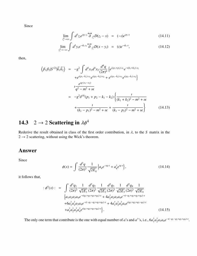
Since

limz0

i→∞

∫d3zieıpi·zi

←→∂ z0

iD(zi − x) = (−ı)eıpi·x (14.11)

limy0

i→−∞

∫d3yie−ıki·yi

←→∂ y0

iD(x − yi) = (ı)e−ıki·x, (14.12)

then,

⟨~p1~p2|S (2)|~k1~k2

⟩= −g2

∫d4x1d4x2

d4q(2π)4

eı(p1+p2)·x1e−ı(k1+k2)·x2

+eı(p1−k1)·x1eı(p2−k2)·x2 + eı(p1−k2)·x1eı(p2−k1)·x2

ıeıq·(x1−x2)

q2 − m2 + ıε

= −g2δ(4)(p1 + p2 − k1 − k2)

ı

(k1 + k2)2 − m2 + ıε

+ı

(k1 − p1)2 − m2 + ıε+

ı

(k1 − p2)2 − m2 + ıε

(14.13)

14.3 2→ 2 Scattering in λφ4

Rederive the result obtained in class of the first order contribution, in λ, to the S matrix in the2→ 2 scattering, without using the Wick’s theorem.

AnswerSince

φ(x) =∫

d3q(2π)3

1√2Eq

aqe−ıq·x + a†qeıq·x

, (14.14)

it follows that,

: φ4(x) : =∫

d3q1

(2π)3

1√

2E1

d3q2

(2π)3

1√

2E2

d3q3

(2π)3

1√

2E3

d3q4

(2π)3

1√

2E4a1a2a3a4e−ı(q1+q2+q3+q4)·x + 4a†1a2a3a4e−ı(−q1+q2+q3+q4)·x

+6a†1a†2a3a4e−ı(−q1−q2+q3+q4)·x + 4a†1a†2a†3a4eı(q1+q2+q3−q4)·x

+a†1a†2a†3a†4eı(q1+q2+q3+q4)·x. (14.15)

The only one term that contribute is the one with equal number of a’s and a†’s, i.e., 6a†1a†2a3a4e−ı(−q1−q2+q3+q4)·x.

Therfore,⟨~p1~p2|S (1)|~k1~k2

⟩= −

ıλ

4!

∫d4x

d3q1

(2π)3

d3q2

(2π)3

d3q3

(2π)3

d3q4

(2π)3

(Ep1 Ep2 Ek1 Ek2

E1E2E3E4

) 12

3!eı(q1+q2−q3−q4)·x⟨0|ap1ap2a

†

1a†2a3a4a†k1a†k2|0⟩. (14.16)

Now, ⟨0|ap1ap2a

†

1a†2a3a4a†k1a†k2|0⟩=

⟨0|ap1ap2a

†

1a†2a3

((2π)3δ(3)(q4 − k1) + a†k1

a4

)a†k2|0⟩

=⟨0|ap1ap2a

†

1a†2a((2π)3(2π)3δ(3)(q4 − k1)δ(3)(q3 − k2)

+a†k2a3(2π)3δ(3)(q4 − k1) + a3a†k1

a†k2a4

)|0⟩

=⟨0|ap1ap2a

†

1a†2|0⟩

(2π)3(2π)3δ(3)(q4 − k2)δ(3)(q3 − k1)

+δ(3)(q4 − k1)δ(3)(q3 − k2). (14.17)

Thus,⟨0|ap1ap2a

†

1a†2a3a4a†k1a†k2|0⟩= (2π)3(2π)3(2π)3(2π)3

δ(3)(p1 − q1)δ(3)(p2 − q2)δ(3)(q3 − k1)δ(3)(q4 − k2) (14.18)

+δ(3)(p1 − q2)δ(3)(p2 − q1)δ(3)(q3 − k1)δ(3)(q4 − k2) + k1 ↔ k2

.

And so,⟨~p1~p2|S (1)|~k1~k2

⟩= −

ıλ

4!

∫d4x

d3q1

(2π)3

d3q2

(2π)3

d3q3

(2π)3

d3q4

(2π)3

(Ep1 Ep2 Ek1 Ek2

E1E2E3E4

) 12

4!eı(q1+q2−q3−q4)·xδ(3)(p1 − q1)δ(3)(p2 − q2)δ(3)(q3 − k1)δ(3)(q4 − k2)

= −ıλ

∫d4xeı(p1+p2−k1−k2)·x

= −ıλ(2π)4δ(4)(p1 + p2 − k1 − k2) (14.19)

14.4 Identities for us(p) and vs(p) SpinorsUse th explicit form of the spinors us(p) and vs(p) for showing∑

s

us(p)us(p) = 6 p + m (14.20)∑s

vs(p)vs(p) = 6 p − m. (14.21)

What normalisation should the spinors have? Show that these identities are consistent with theequations which define the spinors us(p) and vs(p). Are these identities invariant under a changeon the representation of the γ-matrices?

AnswerRemind that

us(p) =√

E + m(χs

~σ·~pE+mχs

)(14.22)

vs(p) =√

E + m(~σ·~p

E+mχs

χs

), (14.23)

where

χ1 =

(10

)χ2 =

(01

). (14.24)

Since~σ · ~p

E + m=

1E + m

(pz px − ıpy

px + ıpy −pz

), (14.25)

then,

u1(p) =√

E + m

10pz

E+mpx+ıpy

E+m

, u2(p) =√

E + m

01

px−ıpy

E+m−

pzE+m

, (14.26)

and

u1(p) =√

E + m(1 0 −

pzE+m −

px+ıpy

E+m

), (14.27)

u2(p) =√

E + m(0 1 −

px−ıpy

E+mpz

E+m

), (14.28)

where the standard representation of Dirac matrices have been used.Similarly,

v1(p) =√

E + m

pz

E+mpx+ıpy

E+m10

, v2(p) =√

E + m

px−ıpy

E+m−

pzE+m01

, (14.29)

and

v1(p) =√

E + m(

pzE+m

px+ıpy

E+m −1 0), (14.30)

v2(p) =√

E + m( px−ıpy

E+m −pz

E+m 0 −1). (14.31)

Now, by simple matrix multiplication, we get,

u1(p)u1(p) =

E + m 0 −pz −px + ıpy

0 0 0 0pz 0 −

p2z

E+m−pz px+ıpz py

E+mpx + ıpy 0 −px pz+ıpy pz

E+m

, (14.32)

u2(p)u2(p) =

0 0 0 00 E + m −px + ıpy pz

0 px + ıpy −p2

x+p2y

E+mpz px−ıpz py

E+m

0 −pzpx pz−ıpy pz

E+m −p2

zE+m

, (14.33)

so that

∑s

us(p)us(p) =

E + m 0 −pz −px + ıpy

0 E + m −px − ıpy pz

pz px − ıpy −E + m 0px + ıpy −pz 0 −E + m

= 6 p + m. (14.34)

Repeating the above process, we get,

∑s

vs(p)vs(p) =

E − m 0 −pz −px + ıpy

0 E − m −px − ıpy pz

pz px − ıpy −E − m 0px + ıpy −pz 0 −E − m

= 6 p − m. (14.35)

From (14.26) and (14.29), we obtain

u†i (p)ui(p) = 2E, v†i (p)vi(p) = 2E, (14.36)

for i = 1, 2.Of course, properties (14.34) and (14.35) are consistent with the equation of motion for spinors

us(p) and vs(p), so that,

(6 p − m)∑

s

us(p)us(p) = (6 p − m)(6 p + m)

= p2 − m2

= 0 (14.37)(6 p + m)

∑s

vs(p)vs(p) = (6 p + m)(6 p − m)

= p2 − m2

= 0, (14.38)

as it was expected from the equation of motion,

(6 p − m)us(p) = 0, (6 p + m)vs(p). (14.39)

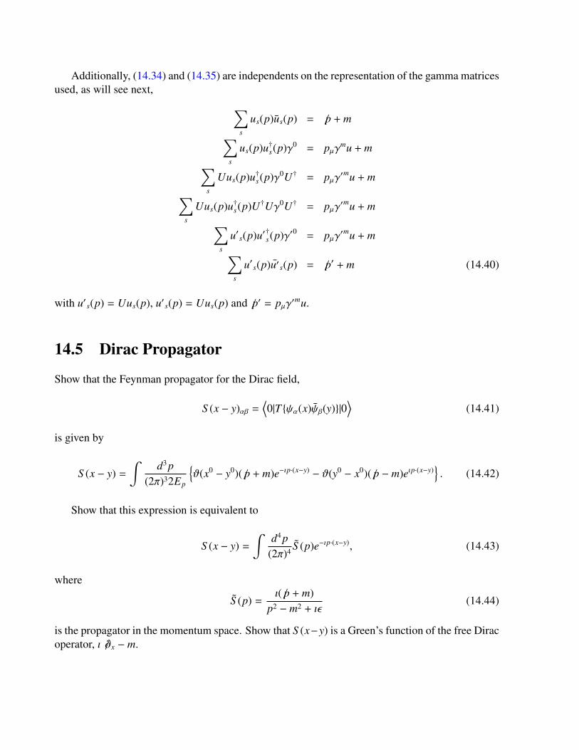
Additionally, (14.34) and (14.35) are independents on the representation of the gamma matricesused, as will see next, ∑

s

us(p)us(p) = 6 p + m∑s

us(p)u†s(p)γ0 = pµγmu + m∑s

Uus(p)u†s(p)γ0U† = pµγ′mu + m∑

s

Uus(p)u†s(p)U†Uγ0U† = pµγ′mu + m∑

s

u′s(p)u′†s(p)γ′0 = pµγ′mu + m∑

s

u′s(p)u′s(p) = 6 p′ + m (14.40)

with u′s(p) = Uus(p), u′s(p) = Uus(p) and 6 p′ = pµγ′mu.

14.5 Dirac Propagator

Show that the Feynman propagator for the Dirac field,

S (x − y)αβ =⟨0|T ψα(x)ψβ(y)|0

⟩(14.41)

is given by

S (x − y) =∫

d3 p(2π)32Ep

ϑ(x0 − y0)(6 p + m)e−ıp·(x−y) − ϑ(y0 − x0)(6 p − m)eıp·(x−y)

. (14.42)

Show that this expression is equivalent to

S (x − y) =∫

d4 p(2π)4 S (p)e−ıp·(x−y), (14.43)

where

S (p) =ı(6 p + m)

p2 − m2 + ıε(14.44)

is the propagator in the momentum space. Show that S (x−y) is a Green’s function of the free Diracoperator, ı 6∂x − m.

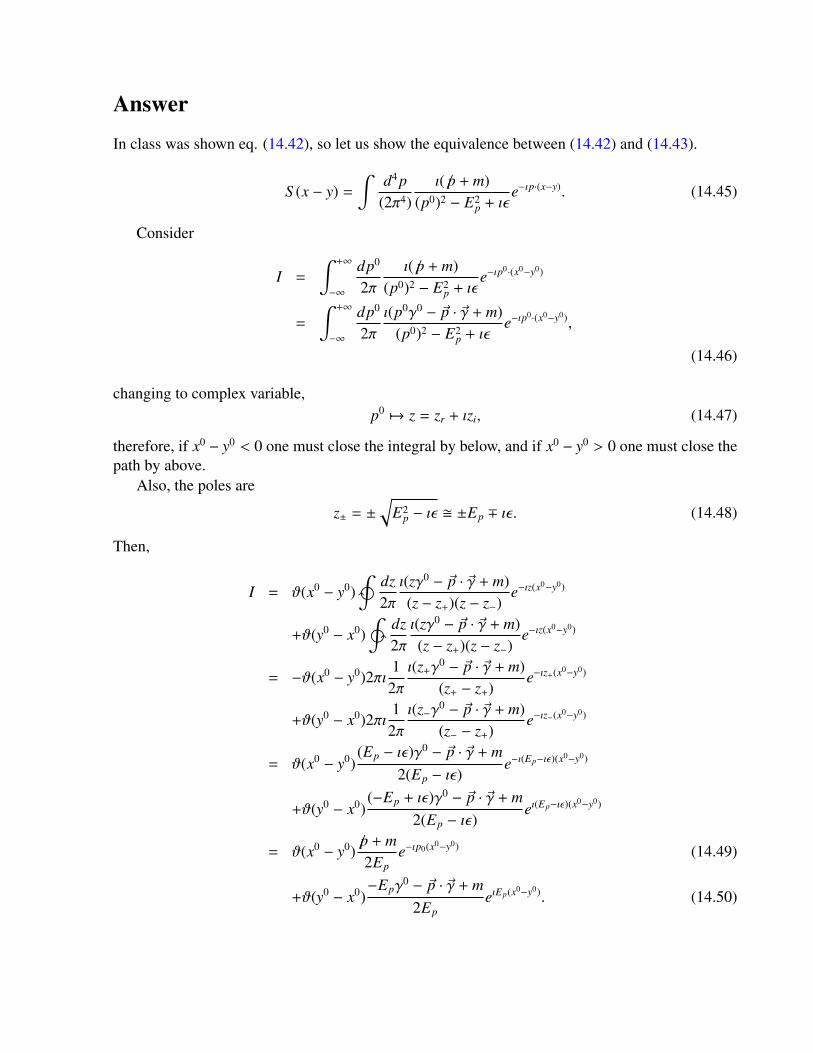
Answer

In class was shown eq. (14.42), so let us show the equivalence between (14.42) and (14.43).

S (x − y) =∫

d4 p(2π4)

ı(6 p + m)(p0)2 − E2

p + ıεe−ıp·(x−y). (14.45)

Consider

I =∫ +∞

−∞

dp0

2πı(6 p + m)

(p0)2 − E2p + ıε

e−ıp0·(x0−y0)

=

∫ +∞

−∞

dp0

2πı(p0γ0 − ~p · ~γ + m)

(p0)2 − E2p + ıε

e−ıp0·(x0−y0),

(14.46)

changing to complex variable,p0 7→ z = zr + ızi, (14.47)

therefore, if x0 − y0 < 0 one must close the integral by below, and if x0 − y0 > 0 one must close thepath by above.

Also, the poles are

z± = ±√

E2p − ıε ±Ep ∓ ıε. (14.48)

Then,

I = ϑ(x0 − y0)

dz2πı(zγ0 − ~p · ~γ + m)(z − z+)(z − z−)

e−ız(x0−y0)

+ϑ(y0 − x0)

dz2πı(zγ0 − ~p · ~γ + m)(z − z+)(z − z−)

e−ız(x0−y0)

= −ϑ(x0 − y0)2πı1

2πı(z+γ0 − ~p · ~γ + m)

(z+ − z+)e−ız+(x0−y0)

+ϑ(y0 − x0)2πı1

2πı(z−γ0 − ~p · ~γ + m)

(z− − z+)e−ız−(x0−y0)

= ϑ(x0 − y0)(Ep − ıε)γ0 − ~p · ~γ + m

2(Ep − ıε)e−ı(Ep−ıε)(x0−y0)

+ϑ(y0 − x0)(−Ep + ıε)γ0 − ~p · ~γ + m

2(Ep − ıε)eı(Ep−ıε)(x0−y0)

= ϑ(x0 − y0)6 p + m2Ep

e−ıp0(x0−y0) (14.49)

+ϑ(y0 − x0)−Epγ

0 − ~p · ~γ + m2Ep

eıEp(x0−y0). (14.50)

Thus,

S (x − y) =∫

d3 p(2π)32Ep

ϑ(x0 − y0)(6 p + m)e−ıp·(x−y) − ϑ(y0 − x0)(6 p − m)eıp·(x−y)

, (14.51)

were in the second term the variable have been change ~p 7→ −~p.Additionally,

(ı 6∂x − m)S (x − y) =∫

d4 p(2π)4 ı

6 p − m)(6 p + mp2 − m2 + ıε

eıp·x

=

∫d4 p

(2π)4 ıp2 − m2 + ıε

p2 − m2 + ıεeıp·x

−

∫d4 p

(2π)4 ııε

p2 − m2 + ıεeıp·x

= ıδ(4)(x − y) + ε(· · · )= ıδ(4)(x − y). (14.52)

Chapter 15... 2nd part

15.1 Kinematic restrictions for scattering and decay processesa. Show that the following processes are not kinematically possible:

• Spontaneous emission of a photon by a free electron.

• A photon absorption by a free electron.

• A pair electron-positron from a single photon.

• A split of a photon into two.

b. Give a general argument that include all the above cases.

c. Obtain the condition that permit the decay of a particle of mass M decay into a triplet ofparticles of masses m1, m2 and m3.

d. Is there any restriction on the masses m1, m2, m3 and m4 in order for scattering 1 + 2 → 3 + 4to occur?

e. Apply the above result to enumerate all permit processes whose initial and final states include,a pair of photons and a couple of electron and/or positron.

Answera.

• Consider a free electron, and choose the CM frame. The energy in this frame is just Ei = m,but after the emission, E f = m + Ke + Eγ > Ei, i.e., this process doesn’t conserve energy andso it’s not allowed.

• Once more choosing the CM. frame, Ei = m + Ke + Eγ > E f = m, therefore it’s not allowed.

197

• In the CM. frame, P f = Pe− + Pe+ = 0, but Pi , 0 because mγ = 0.

• This last process can (eventually) conserve both, energy and momentum, but doesn’t con-serve helicity, so it’s neither allow.

b. As it was seen in the above examples, processes of three particles which involve at least amassless one, are not kinematically allowed.

c. In order for a particle of mass M to decay into a triplet of particles with masses m1, m2 and m3,energy and momentum must be conserved. It can be seen from the CM frame as

m1 + T1 + m2 + T2 + m3 + T3 = M, (15.1)~p1 + ~p2 + ~p3 = 0, (15.2)

where ~pi are the momenta of the particles after the decay.

d. From the CM frame, the restriction to a 2→ 2 particles process is given by

m1 + T + m2 + T2 = m3 + T3 + m4 + T4 (15.3)

if the particles are massive.If one of they is massless, the process is not allowed because of momentum (and helicity)

conservation. Thus, a pair number of photons must be involved.

e.

15.2 Bhabha scatteringFor the Bhabha scattering, e− + e+ → e− + e+,

a. Show that the lower order contribution to the S matrix corresponding to this process is

S (2)(e− + e+ → e− + e+) = S a + S b, (15.4)

with

S a = −e2∫

d4x1d4x2 :(ψ−γµψ+

)x1

(ψ+γνψ−

)x2

: Dµν(x1 − x2) (15.5)

S b = −e2∫

d4x1d4x2 :(ψ−γµψ−

)x1

(ψ+γνψ+

)x2

: Dµν(x1 − x2). (15.6)

b. From (15.5) and (15.6) get the Feynman amplitude for the process

e+(p1, s1) + e−(p2, s2)→ e+(p′1, s′1) + e−(p′2, s

′2). (15.7)

Answera. For QED, the interaction Hamiltonian is

HI = −e : ψ 6Aψ : . (15.8)

Obviously, for just fermionic initial and final states⟨~p1 ~p2

∣∣∣S (1)∣∣∣ ~k1 ~k2

⟩= 0. (15.9)

Then, the first non-trivial contribution to the S matrix is second order on e,⟨~p1 ~p2

∣∣∣S (2)∣∣∣ ~k1 ~k2

⟩,

withS (2) = −e2

∫d4x1d4x2T

: (ψ 6Aψ)x1 :: (ψ 6Aψ)x2 :

(15.10)

For the Bhabha scattering, no photons are involved at initial or final state, so the only possibilityis that they’d be contracted, i.e.,

S (2) = −e2∫

d4x1d4x2 : (ψγµψ)x1(ψγνψ)x2 : Dµν(x1 − x2), (15.11)

butψ = ψ+ + ψ− and ψ = ψ+ + ψ−. (15.12)

Since, ψ+ annihilates an electron, ψ− creates a positron, ψ− annihilates an electron and ψ+

creates a positron, the set up should have all them once. It gives 4 different possibilities,

1. (ψ−γµψ−)x1(ψ+γνψ+)x2

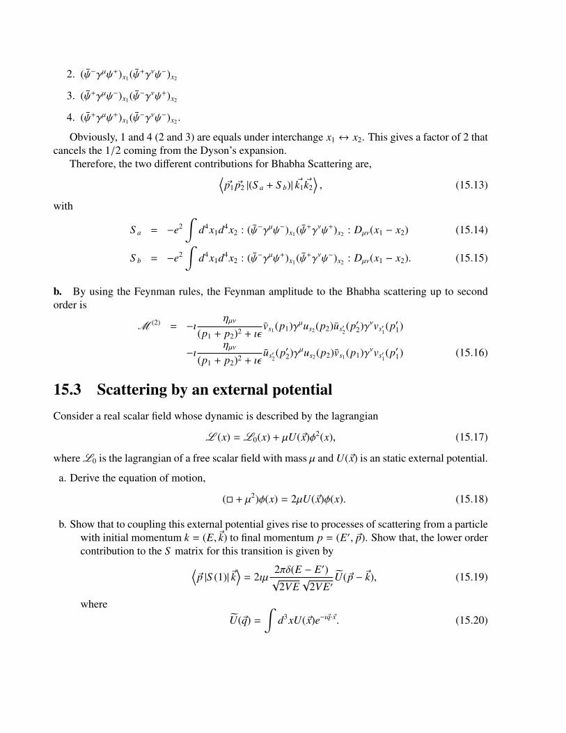
2. (ψ−γµψ+)x1(ψ+γνψ−)x2

3. (ψ+γµψ−)x1(ψ−γνψ+)x2

4. (ψ+γµψ+)x1(ψ−γνψ−)x2 .

Obviously, 1 and 4 (2 and 3) are equals under interchange x1 ↔ x2. This gives a factor of 2 thatcancels the 1/2 coming from the Dyson’s expansion.

Therefore, the two different contributions for Bhabha Scattering are,⟨~p1 ~p2 |(S a + S b)| ~k1 ~k2

⟩, (15.13)

with

S a = −e2∫

d4x1d4x2 : (ψ−γµψ−)x1(ψ+γνψ+)x2 : Dµν(x1 − x2) (15.14)

S b = −e2∫

d4x1d4x2 : (ψ−γµψ+)x1(ψ+γνψ−)x2 : Dµν(x1 − x2). (15.15)

b. By using the Feynman rules, the Feynman amplitude to the Bhabha scattering up to secondorder is

M (2) = −ıηµν

(p1 + p2)2 + ıεvs1(p1)γµus2(p2)us′2

(p′2)γνvs′1(p′1)

−ıηµν

(p1 + p2)2 + ıεus′2

(p′2)γµus2(p2)vs1(p1)γνvs′1(p′1) (15.16)

15.3 Scattering by an external potentialConsider a real scalar field whose dynamic is described by the lagrangian

L (x) = L0(x) + µU(~x)φ2(x), (15.17)

where L0 is the lagrangian of a free scalar field with mass µ and U(~x) is an static external potential.

a. Derive the equation of motion,

( + µ2)φ(x) = 2µU(~x)φ(x). (15.18)

b. Show that to coupling this external potential gives rise to processes of scattering from a particlewith initial momentum k = (E,~k) to final momentum p = (E′, ~p). Show that, the lower ordercontribution to the S matrix for this transition is given by⟨

~p |S (1)|~k⟩= 2ıµ

2πδ(E − E′)√

2VE√

2VE′U(~p − ~k), (15.19)

whereU(~q) =

∫d3xU(~x)e−ı~q·~x. (15.20)

AnswerIn order to get the eqs. of motion, one apply the Euler-Lagrange eqs.,

∂µ

(∂L

∂(∂µφ

)= ∂µ∂

µφ, (15.21)

and∂L

∂φ= −µ2φ + 2µU(~x)φ, (15.22)

so,( + µ2)φ(x) = 2µU(~x)φ(x). (15.23)

Since LI is time-independent, then

HI(x) = −µU(~x) : φ2(x) : . (15.24)

The initial and final states are obtained from the vacuum via

|~k > =√

2Ea†k |0 > (15.25)

|~p > =√

2E′a†p|0 > . (15.26)

Also, the Dyson expansion for the S matrix is,

S = 1 + (−ı)∫

d4xHI(x) +(−ı)2

2!

∫dxd4yT HI(x)HI(y) + · · · , (15.27)

therefore, for (15.24) and ~p , ~k, one get,⟨~p |S (1)|~k

⟩= ıµ

√2E√

2E′∫

d4xU(~x)⟨0∣∣∣ap : φ2(x) : a†k

∣∣∣ 0⟩= ıµ lim

z0→∞lim

y0→∞

∫d4xd3zd3yeıp·ze−ık·y

←→∂ z0←→∂ y0U(~x)

⟨0∣∣∣φ(z) : φ2(x) : φ(y)

∣∣∣ 0⟩= ıµ lim

z0→∞lim

y0→∞

∫d4xd3zd3yeıp·ze−ık·y

←→∂ z0←→∂ y0U(~x)2D(z − x)D(x − y)

= 2ıµ∫

d4xeıp·xe−ık·xU(~x)

= 2ıµ∫

d3xe−ı(~p−~k)·~xU(~x)∫

dx0eı(E−E′)x0

= 2ıµ(2π)δ(E − E′)U(~p − ~k). (15.28)

Note that if the particle state is defined by

|~p >= a†p|0 >, (15.29)

the result would be ⟨~p |S (1)|~k

⟩= 2ıµ

(2π)δ(E − E′)√

2E√

2E′U(~p − ~k). (15.30)

15.4 Feynman rules for a pseudo-scalar mesons theoryConsider a theory for pseudo-scalar mesons, defined by the lagrangian

L (x) = L0(x) +Lint(x), (15.31)

where

L0 =12∂µφ∂

µφ −µ2

2φ2 + ψ(ı 6∂ − m)ψ, (15.32)

andLint = −ıgψγ5ψφ. (15.33)

Use the similarity between this theory and QED for writing its Feynman rules.

AnswerRemind that in order to construct the Feynman diagram, one assign different lines to different sortof particles, i.e., two kind of propagators in the described set up, say, straight lines for fermionsand dashed ones for scalar field. Also, the vertex is a convergent point of as many propagators asthe order of the interaction.

Next are listed the Feynman rules for the set up theory.

1. Draw all graphs with a given number of vertices, n. Remember, fermion lines are orientedand are closed or infinite (it means begin and end at ±∞).

2. For each vertex, write a factor gγ5.

3. For each internal bosonic line, labelled by the momentum k, write a factor

D(k) =i

k2 − µ2 + ıε. (15.34)

4. For each internal fermion line, labelled by the momentum p, write a factor

S (p) = ı6 p + m

p2 − m2 + ıε. (15.35)

5. Add one of the following factors for each external line:

• initial electron: us(p).

• initial positron: vs(p).

• final electron: us(p).

• final positron: vs(p).

Also each external boson has an associated momentum.

6. The spinor factors for each fermion line are ordered so that, reading from right to left, theyoccur in the same sequence as following the fermion line in the direction of its arrow.

7. For each fermion loop, take trace and multiply by a factor (−1).

8. For each momentum, q, which is not fixed by energy-momentum conservation, carry out theintegration

1(2π)4

∫d4q.

9. Multiply the expression by a phase factor δP which is equal to +1 or -1 if an ever or oddnumber of interchanges of neighboring fermion operators is required to write the fermionoperators in the correct normal order.

The above rules give the Feynman amplitude, M (n), of order n (number of vertices). From here,the n-th order of the S matrix is given by⟨

f∣∣∣S (n)

∣∣∣ i⟩ = (2π)4δ(4)(P f − Pi)M (n). (15.36)

Chapter 16QFT II 3

16.1 γ − γ ScatteringUnlike classical electrodynamics, QED predicts that a couple of light shafts that cross, suffer certainscattering,

a. Identify and write down the lower order, in the Dyson expansion for the S -matrix, whichallows the process 2γ → 2γ. Write it as compact as possible, having special care with thefinal coefficients.

b. Draw the Feynman diagrams -in the momentum space- associated to the above process, and byusing the Feynman rules write the expression of the Feynman amplitude.

AnswerSince,

HI = −e∫

d3x : ψ 6Aψ :, (16.1)

and we have four photons in both, initial and final states, in order to get a non-trivial contributionwe must consider the Dyson expansion to order fourth,

〈 f |S |i〉 =(ıe)4

4!

∫d4x1d4x2d4x3d4x4⟨

f |T: (ψ 6Aψ)x1 :: (ψ 6Aψ)x2 :: (ψ 6Aψ)x3 :: (ψ 6Aψ)x4 :

|i⟩

=(ıe)4

4!1

2VEp1

12VEp2

12VEp3

12VEp4

εµ(p1)εν(p2)ε∗λ(p3)ε∗ρ(p4)∫d4x1d4x2d4x3d4x4eıp1·x1eıp2·x2eıp3·x3eıp4·x4⟨

f |T: (ψγµψ)x1 :: (ψγνψ)x2 :: (ψγλψ)x3 :: (ψγρψ)x4 :

|i⟩. (16.2)

205

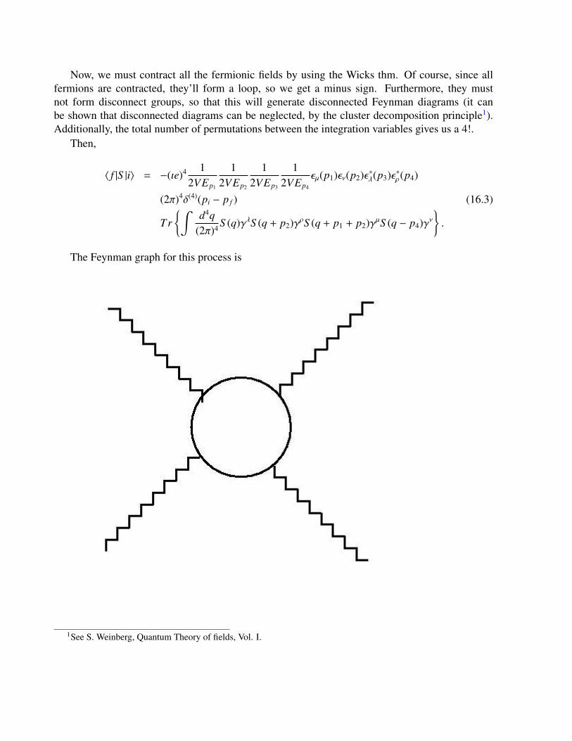
Now, we must contract all the fermionic fields by using the Wicks thm. Of course, since allfermions are contracted, they’ll form a loop, so we get a minus sign. Furthermore, they mustnot form disconnect groups, so that this will generate disconnected Feynman diagrams (it canbe shown that disconnected diagrams can be neglected, by the cluster decomposition principle1).Additionally, the total number of permutations between the integration variables gives us a 4!.

Then,

〈 f |S |i〉 = −(ıe)4 12VEp1

12VEp2

12VEp3

12VEp4

εµ(p1)εν(p2)ε∗λ(p3)ε∗ρ(p4)

(2π)4δ(4)(pi − p f ) (16.3)

Tr∫

d4q(2π)4 S (q)γλS (q + p2)γρS (q + p1 + p2)γµS (q − p4)γν

.

The Feynman graph for this process is

1See S. Weinberg, Quantum Theory of fields, Vol. I.

Clearly, from the diagram it follows that

M = −(ıe)4εµ(p1)εν(p2)ε∗λ(p3)ε∗ρ(p4)

Tr∫

d4q(2π)4 S (q)γλS (q + p2)γρS (q + p1 + p2)γµS (q − p4)γν

(16.4)

16.2 Rutherford’s scatteringPeskin-Shoeder problem 4.4

AnswerSince

ψ+(x)|e−(~p, s) >= |0 >1

(2VEp)1/2 us(p)e−ıp·x, (16.5)

it follows that, at first order in perturbations,⟨p′

∣∣∣∣∣ıe ∫d4x : ψγµψ : Aµ

∣∣∣∣∣ p⟩=

⟨p′

∣∣∣∣∣ıe ∫d4x : ψ−γµψ+ : Aµ

∣∣∣∣∣ p⟩

= ıe1√

2VEp

1√2VEp′

us′(p′)γmuus(p)∫

d4xe−ı(p−p′)·xAµ

= ıe1√

2VEp

1√2VEp′

us′(p′)γmuus(p)Aµ(p − p′). (16.6)

If Aµ does not depend on t,⟨p′

∣∣∣∣∣ıe ∫d4x : ψγµψ : Aµ

∣∣∣∣∣ p⟩= ıeAµ(~p − ~p′)2πδ(E − E′)

1√2VEp

1√2VEp′

us′(p′)γµus(p). (16.7)

Now, the cross-section for this process is given by

dσ =1vi

12Ei

d3 p f

(2π)32E f|M (pi → p f )|2(2π)δ(Ei − E f ), (16.8)

it can be written as,

dσ =1vi

12Ei

|p f |2d|p f |dΩ

(2π)32E f|M (pi → p f )|2(2π)δ(Ei − E f ). (16.9)

Since,

δ(F(x) − F(x0)) =1

|F′(x0)|δ(x − x0), (16.10)

anddE f

d|p f |=

p f

E f, (16.11)

then, we can integrate over the modulus of the momentum,∫|p f |

2d|p f |

(2π)32E f2πδ(Ei − E f ) =

pi

(2π)2

12. (16.12)

Thus,

dσ =1

2(2π)2

pi

vi

12Ei|M |2dΩ, (16.13)

next, we’ll use the equationEi =

pi

vi, (16.14)

we get,

dσ =1

(4π)2 |M |2dΩ. (16.15)

Let’s now restrict ourselves to the Coulombian potential,

A0 =Ze4π

1r. (16.16)

Therefore,

dσdΩ

=1

(4π)2 |M |2

=

(e2

4π

)2

Z2 1

|~p − ~p′|412

∑r,s

|ur(p′)γ0us(p)|2

=12

(αZ)|~q|4

tr(6p′γ0 6pγ0) + m21

=

12

(αZ)|~q|4

trp′µpν(γµγ0γνγ0) + m21

=

12

(αZ)|~q|4

4p′µpν(2ηµ0ην0 − ηµν) + 4m2

= 2

(αZ)|~q|4

(m2 + E2 + ~p · ~p′

). (16.17)

In the above calculations, we’ve used the relations∑s

us(p)us(p) = 6p + m (16.18)

tr(γµγνγλγρ) = 4[ηµνηλρ − ηµληρν + ηµρηνλ

]. (16.19)

Finally, by using

~p · ~p′ = |p| cos θ, (16.20)

and

|~p − ~p′|2 = 2|p|2(1 − cos θ) = 4|p|2 sin2(θ/2), (16.21)

we obtain,

dσdΩ

=18

(αZ)2

|p|4(m2 + E2 + |p|2 cos θ)

sin4(θ/2)

=14

(αZ)2

E2v4

(1 − v2 sin2(θ/2))sin4(θ/2)

. (16.22)

In the non-relativistic case, v 1 and E2 m2, then

dσdΩ=

14

(αZ)2

E2v4

1sin4(θ/2)

. (16.23)

16.3 Crossing symmetry

a. Draw the Feynman diagrams, at tree level, in the momentum space for e+(p2) + e−(p1) →(k1) + γ(k2). Use the Feynman rules in order to write the Feynman amplitudes associated toeach diagram.

b. Draw the Feynman diagrams, at tree level, in the momentum space for e− + γ → e− + γ. Usethe Feynman rules in order to write the Feynman amplitudes associated to each diagram.

c. Show that the amplitudes of each one of the diagrams of the annihilation (a.) can be obtainedfrom the ones of the Compton effect (b.) through certain identification of the momentumvariables.

d. Explain what crossing symmetry consist on.

Answer

And from the diagrams,

Ma1 = (ıe)2vr(p2)γµS (p1 − k1)γνus(p1)ε∗µ(k2)ε∗ν(k1) (16.24)

Mb1 = (ıe)2vr(p2)γµS (p1 − k2)γνus(p1)ε∗µ(k1)ε∗ν(k2) (16.25)

Ma2 = (ıe)2ur(p2)γµS (p1 + k1)γνus(p1)ε∗µ(k2)εν(k1) (16.26)

Mb2 = (ıe)2ur(p2)γµS (p1 − k2)γνus(p1)εµ(k1)ε∗ν(k2). (16.27)

Let’s change p2 7→ −p2 and k1 7→ −k1 in the amplitudes M1, then,

M ′a1 = (ıe)2vr(−p2)γµS (p1 + k1)γνus(p1)ε∗µ(k2)ε∗ν(−k1) (16.28)

M ′b1 = (ıe)2vr(−p2)γµS (p1 − k2)γνus(p1)ε∗µ(−k1)ε∗ν(k2). (16.29)

But the eq. of motion for spinos are,

(6p + m)us(p) = 0 (16.30)(− 6p + m)vs(p) = 0, (16.31)

in the above equations, we can change us(−p) by vs(p). Additionally, the polarization of a photonis complex just if it’s elliptically polarised, therefore, under a change in the momentum k 7→ −k,also the orientation of the polarization must change, i.e.,

εµ(k) = ε∗µ(−k). (16.32)

Finally, we get

M ′a1 = (ıe)2ur(p2)γµS (p1 + k1)γνus(p1)ε∗µ(k2)εν(k1) (16.33)

M ′b1 = (ıe)2ur(p2)γµS (p1 − k2)γνus(p1)εµ(k1)ε∗ν(k2), (16.34)

that are nothing but the Feynman amplitudes for the Compton scattering.Let’s try now of explaining what this crossing symmetry is.Both process, e+ + e− → 2γ and Compton scattering, (at tree level) are obtained from the

second order expansion of the S -matrix for QED. Nonetheless, for each process we decide to takethe positive or negative frecuency part of the fields, depending on the initial and final particles ofthe process. Since the total numbers of photons and leptons are the same, the Feynman graph for aprocess can be obtained from the topologically equivalents Feynman diagrams of the other, ’causeit’s just a different choice of the positive and negative frecuency of the field. Furthermore, thecombinatoric ceofficients are equal for both processes.

In the crossing symmetry, just as we’ve seen, if we take a lepton from initial to final (or vicev-ersa) we should change the particle by it’a anti-particle. Similarly, if we change a photon, weshould change it polarization.

Chapter 17QGT II 4

17.1 Relativistic form for the flux factor

AnswerConsider

I =√

(~p1 · p2)2 − m21m2

2, (17.1)

then, for p1 = (E2, ~p1) and p2 = (E2, ~p2), it follows that,

I =√

(E1E2 − ~p1 · ~p2)2 − (E21 − ~p

21)(E2

2 − ~p22)

=

√(~p1 · ~p2)2 − 2E1E2((~p1 · ~p2) − ~p2

1~p22 + E2

1~p2 + E22~p1

= E1E2

√(~v1 − ~v2)2 − (~v1 × ~v2)2. (17.2)

From (17.1), I is a Lorents invariant, therefore (17.2) is so. Furthermore, the density transformas a zeroth component of a 4-vector, as the energy, thus, if (17.2) is a lorentz invariant, I′ =n1n2

√(~v1 − ~v2)2 − (~v1 × ~v2)2 is also a Lorentz invariant.

in the CM. frame, where p1 = (E, ~p) and p2 = (E′,−~p),

I =√

(EE′ + |~p|2)2 − ((E2 − |~p|2)(E′2 − |~p|2))

=

√E2E′2 + |~p|4 + 2|~p|2EE′ − E2E′2 − |~p|4 + |~p|2(E2 + E′2)

= |~p|√

s. (17.3)

17.2 Two bodies phase space in the lab frameMaggiore, 6.2.

213

Answer

Since the velocity of the second particle in the initial frame is v2, we should boost our set up by

gamma(v2) =1√

1 − v22

, (17.4)

then,

V2,lab =v2 − v2

1 − v22

= 0. (17.5)

Also,

Elab = γ2(E′ + v2 p′x)= γ2(E′ + v2|p′| cos(θ)). (17.6)

Thus,dElab = γ2v2|p′|d(cos(θ)). (17.7)

Moreover,

dΦ(2)CM =

116π2

|~p′|√

sdΩ

=1

16π2

|~p′|√

sdφd(cos(θ)), (17.8)

next, by integrate on φ, we get,

dΦ(2)lab =

dElab

8πγ2v2√

s. (17.9)

17.3 Elastic e−µ− scattering

Mandl and Shaw, 8.2.

Answer

17.4 High energy elastic e−e− scattering

Mandl and Shaw, 8.6.

AnswerIn here we’ll work on the CM. frame, then

dσ =14I|Ma +Mb|

2dΦ(2)

=1

64π2s14|Ma +Mb|

2dΩ, (17.10)

where,

Ma = −ıe2

(p1 − p′1)2 ur1(p′1)γµus1(p1)ur2(p′2)γµus2(p2) (17.11)

Mb = ıe2

(p1 − p′2)2 ur2(p′2)γµus1(p1)ur1(p′1)γµus2(p2), (17.12)

where the index 1 and 2 denote electrons and muons respectively, and also prime variables denotefinal momentum. Bellow, we’ll drop all contribution coming from electron mass because E me.

Note that,|Ma +Mb|

2 = |Ma|2 + |Mb|

2 +M ∗a Mb +MaM

∗b , (17.13)

then,

14|Ma|

2 =e4

4[(p1 − p′1)2]2

∑si,ri

ur1(p′1)γµus1(p1)us1(p1)γνur1(p′1)

ur2(p′2)γµus2(p2)us2(p2)γνur2(p′2) (17.14)

=e4

4[(p1 − p′1)2]2 Tr(6p′1γµ 6p1γ

ν)Tr(6p′2γµ 6p2γ

ν) (17.15)

Part VI

Appendixes

217

Chapter 18Geometry: Conics

This chapter gain importance when one is interested in Kepler’s problem, i.e., a particle in a poten-tial U(~r) ∼ |~r|−1. Here we give a brief review of conics, further treatment can be found in a bookon analytical geometry.

18.1 CircumferenceA circumference is described by the equation1

x2 + y2 = R2, (18.1)

where R is the radius.

18.2 Ellipse

An ellipse is described by the equation,

x2

a2 +y2

b2 = 1, (18.2)

with a and b the major and minor radii, respectively2, i.e., a > b. Foci lie at the major diameter ata distance c, such that, c2 = a2 − b2. eccentricity, ε, is defined by

ε =ca. (18.3)

Obviously, for a circumference ε = 0.We can also characterize a point on the ellipse by the radii from the foci,

r1 = a + εx, r2 = a − εx. (18.4)1Next we consider just figures centered at the origin of coordinates, without lost of generality.2We’ve chosen the large side of the ellipse oriented in x-axis.

219

18.3 Hyperbola

A hyperbola is described by the equation

x2

a2 −y2

b2 = 1, (18.5)

where a is the distance from the origin to the vertice and b such that the hyperbola goes asymptot-ically as

y = ±ba

x. (18.6)

The foci are located at c =√

a2 + b2, again the eccentricity is ε = ca but now since c > a ⇒ ε > 1.

In term of the focal radii,r1 = a + εx, r2 = a − εx. (18.7)

18.4 Parabola

A parabola is described by the equation

y2 = 2px, (18.8)

where focus is located at p/2 from the vertice. The focal radius is r = x + p/2 and eccentricity isε = 1.

18.5 Conics in polar coordinates

All the conics named before can be written in polar coordinates by the equation

ρ =p

1 − ε cos θ. (18.9)

Chapter 19Special Functions

Special functions play an important rôle when one wants to solve the equation of motion forcertain systems, of course we don’t pretend nor try to cover the subject, but showing a punctualuseful formulae such as definitions, special values and so on.

19.1 Gamma Function

Integral forms for the gamma function are

Γ(z) =∫ ∞

0dte−ttz−1 (19.1)

= xz∫ ∞

0dte−xttz−1 (19.2)

=

∫ ∞

0dt ln(t)e−t(t − z)ez−1 (19.3)

=

∫ ∞

−∞

dt exp(zt − et). (19.4)

Also,

Γ

(12

)=√π, Γ

(−

12

)= −2

√π, Γ(n + 1) = nΓ(n). (19.5)

19.2 Beta Function

221

Beta function can be defined in integral form by

β(x) =∫ 1

0dt

tx−1

1 + t(19.6)

=

∫ ∞

0dt

e−xt

1 + e−t . (19.7)

There exists the beta function for two parameters, defined by

B(x, y) =∫ 1

0dttx−1(1 − t)y−1 (19.8)

=Γ(x)Γ(y)Γ(x + y)

(19.9)

= B(y, x). (19.10)

19.3 Bessel Functions

Bessel functions are solutions to the ordinary differential equation

d2

dx2 Zν(x) +1x

ddx

Zν(x) +(1 −

ν2

x2

)Zν(x) = 0. (19.11)

They have a lot of properties that we won’t discuss here.

19.4 Associated Legendre Polynomials

Associated Legendre polynomials are solutions to the ordinary differential equation

(1 − x2)ddx

Pµν(x) − 2x

ddx

Pµν(x) +

(ν(ν + 1) −

µ2

1 − x2

)Pµν(x) = 0. (19.12)

Legendre polynomials are the particular case µ = 0, and they are defined by the relation

Pν(x) =1

2νν!dν

dxν(x2 − 1)ν. (19.13)

Also,

Pµν(x) = (−1)µ(1 − x2)µ/2

dµ

dxµPν(x). (19.14)

19.5 Hermite Polynomials

Hermite polynomials are the solution to the ordinary differential equation

d2

dx2 Hn(x) − 2xddx

Hn(x) + 2nHn(x) = 0. (19.15)

Their Rodrigues’ formula is

Hn(x) = (−1)nex2 dn

dxn e−x2, (19.16)

and they’re a basis for the L2(x) satisfying∫ ∞

−∞

dxe−x2Hn(x)Hm(x) =

0; m , n

√π2nn!; m = n (19.17)

19.6 Laguerre polynomials

Laguerre polynomials are solution to the ordinary differential equation

xd2

dx2 Lαn (x) + (α + 1 − x)ddx

Lαn (x) + nLαn (x) = 0. (19.18)

Their Rodrigues’ formula is

Lαn (x) =1n!

exx−αdn

dxn

(e−xxα

)(19.19)

=

n∑m=0

(−1)m

(n + αn − α

)xm

m!(19.20)

They’re also a basis for L2(x), and its orthogonality is given by∫ ∞

0dxe−xxαLαm(x)Lαn (x) =

0; m , n(

n+αn

)Γ(1 + α); m = n

. (19.21)

Bibliography

[1] Marcelo Alonso and Edward J. Finn. Física, volume Volumen II: Campos y Ondas. FondoEducativo Interamericano, 1976.

[2] Marcelo Alonso and Edward J. Finn. Física, volume Volumen I: Mecánica. Addison-WesleyIberoamericana, 1986.

[3] Leopoldo García-Colín Scherer. Termodinámica Estadísca. Universidad AutónomaMetropolitana, 1995.

[4] Herbert Goldstein, Charles Poole, and John Safko. Classical Mechanics. Addison-Wesley,2000.

[5] Walter Greiner. Classical Electrodynamics. Springer, 1998.

[6] Walter Greiner, Ludwig Neise, and Horst Stöcker. Thermodynamics and Statistical Mechan-ics. Springer, 1997.

[7] David J. Griffiths. Introduction to Electrodynamics. Prentice Hall, 1999.

[8] Kerson Huang. Statistical Mechanics. Wiley, 1987.

[9] John David Jackson. Classical Electrodynamics. Wiley, 1999.

[10] R. K. Pathria. Statistical Mechanics. Butterworth Heinemann, 1996.

[11] F. Reif. Fundamental of Statistical and Thermal Physics. McGraw-Hill, 1965.

[12] Lim Yung-Kuo, editor. Problems and Solutions on Electromagnetism. World Scientific, 1993.

[13] Lim Yung-Kuo, editor. Problems and Solutions on Thermodynamics and Statistical Mechan-ics. World Scientific, 1996.

225

List of Figures

2.1 It shows the Bessel functions J0 (in blue) and J1 (in red). . . . . . . . . . . . . . . 33

4.1 Magnetic dipole in front a superconductor. . . . . . . . . . . . . . . . . . . . . . . 49

9.1 Classical Scattering . . . . . . . . . . . . . . . . . . . . . . . . . . . . . . . . . . 1089.2 Gas enclosed on a box is escaping very slowly, so the process is almost in equilibrium.1119.3 Propagation of a sound wave through a tube . . . . . . . . . . . . . . . . . . . . . 1169.4 Dual lattice . . . . . . . . . . . . . . . . . . . . . . . . . . . . . . . . . . . . . . 126

10.1 A drawn of a circle of radius 4 in a lattice. The black dot represent the centre andthe blue ones are the circumference. . . . . . . . . . . . . . . . . . . . . . . . . . 150

227

List of Tables

9.1 Thermal conductivity (cal/cm2 − s)/(C/cm)) . . . . . . . . . . . . . . . . . . . . 118

229

problem book - .:: · pdf fileproblem book oscar castillo-felisola july 25, 2007. ... iii...

Documents