probing the physics of slip–stick friction using a …jw12/jw pdfs/schumacher_garoff2.pdf · the...

Probing the Physics of Slip–Stick Frictionusing a Bowed String

R. T. SchumacherPhysics Department, Carnegie Mellon University, Pittsburgh,Pennsylvania, USA

S. GaroffPhysics Department and Center for Complex Fluids Engineering,Carnegie Mellon University, Pittsburgh, Pennsylvania, USA

J. WoodhouseCambridge University Engineering Department, Cambridge, UK

Slip–stick vibration driven by friction is important in many applications, and tomodel it well enough to make reliable predictions requires detailed informationabout the underlying physical mechanisms of friction. To characterize the frictionalbehavior of an interface in the stick–slip regime requires measurements that them-selves operate in the stick–slip regime. A novel methodology for measurements ofthis kind is presented, based on the excitation of a stretched string ‘‘bowed’’ witha rod that is coated with the friction material to be investigated. Measurements ofthe motion of the string allow the friction force and the velocity waveform at the con-tact point to be determined by inverse calculation. These friction results can be cor-relatedwithmicroscopic analysis of thewear track left in the coated surface. Resultsare presented using rosin as a frictionmaterial. These show that ‘‘sticking’’ involvessome temperature-dependent shear flow in the friction material, and that the exactdefinition of the states of ‘‘sticking’’ and ‘‘slipping’’ is by nomeans clear-cut. Frictionforce during slipping shows complex behavior, not well correlated with variationsin sliding speed, so that other state variables such as temperature near the interfacemust play a crucial role. A new constitutive model for rosin friction, based on therepeated formation and healing of unstable shear bands, is suggested.

Keywords: Adhesion; Creeping friction; Friction-driven autonomous oscillations;Interfacial friction; Kinetic friction; Stick–slip oscillation

Received 14 October 2004; in final form 15 March 2005.One of a collection of papers honoring Manoj K. Chaudhury, the February 2005

recipient of The Adhesion Society Award for Excellence in Adhesion Science, sponsoredby 3M.

Address correspondence to Robert T. Schumacher, Department of Physics, CarnegieMellon University, Pittsburgh, PA 15213, USA. E-mail: [email protected]

The Journal of Adhesion, 81:723–750, 2005

Copyright # Taylor & Francis Inc.

ISSN: 0021-8464 print=1545-5823 online

DOI: 10.1080/00218460500187715

723

INTRODUCTION

The measurement of friction force at an interface can be important formany reasons, from understanding the fundamental physics of frictionto characterizing the friction and wear properties of particular inter-faces relevant to machines and other applications. For many of theseapplications, ranging from vehicle brakes through microelectromecha-nical systems (MEMS) to the strings of a violin, one reason for interestin friction is that vibration may be caused by frictional interaction(see, for example, references 1 and 2). This vibration may be wantedor unwanted, but in either case there is a need to understand, predict,and control it. Engineering-based problems of this kind may seemrather old-fashioned by comparison with the novel applications to,for example, rock mechanics or biological systems, which have beenthe focus of much attention in recent friction research (see, forexample, references 3 and 4). However, many unsolved problemsremain in this area that are significant both for fundamental physicalunderstanding and for technological applications.

Characterizing the constitutive law that determines the frictionforce currently presents the greatest challenge in modeling friction-driven vibration. In many technological disciplines it is still commonto assume extremely naive models of friction, which when subjectedto experimental scrutiny turn out not to give predictions that are suffi-ciently reliable for design purposes. In recent years various more-sophisticated friction models have been proposed (such as the ‘‘rateand state’’ models, see, for example, references 4 and 5) that give abetter qualitative match to observed frictional behavior in certain set-tings. However, when detailed tests have been made it has generallybeen found that none of these models is yet capable of quantitativeprediction of the stability threshold and transient details of frictionallyexcited vibration, especially when it occurs at high frequency [2, 6–9].For example, to the best of the authors’ knowledge it is not possible touse any current finite-element package to obtain reliable predictions ofwhen a vehicle braking system will squeal.

There are many ways to measure friction. Most types of apparatusare designed to impose a state of steady sliding and then determinethe resulting shear force across the interface. (The words ‘‘slipping’’and ‘‘sliding’’ are used interchangeably.) Factors such as pressure,temperature, and humidity may be varied to give a fuller characteriza-tion of the tribological behavior. However, if one’s aim in charac-terizing friction is to predict and control friction-excited vibration,then such a strategy is inadequate. The friction force during self-excited vibration, often at kilohertz frequencies, will in general behave

724 R. T. Schumacher et al.

differently from anything one might deduce from steady-sliding mea-surements (see, for example, references 6 and 9). To obtain sufficientdata to motivate, validate, and calibrate accurate constitutive laws itis necessary to augment steady-sliding tests with controlled measure-ments using an apparatus that itself operates in the stick–slip regime,or which imposes some other high-frequency dynamic variation. Suchmeasurements pose new challenges to the experimenter. No singleapparatus can be expected to provide all the necessary information,and this article describes one promising recent approach that comple-ments other methods.

A bowed violin string is a familiar example of vibration excited byfriction. In a musical context, the friction behavior is given and themusician is interested in what kind of string motions, and hencesounds, can be produced. In this work, we turn the idea around. Usingan apparatus based on a well-characterized stretched string excited bya ‘‘bow’’ coated with a layer of the friction material to be studied, obser-vations of the string motion are used to infer the friction force, which ishard to measure directly under these interfacial conditions. The evi-dence from the measurement of friction force can be supplementedby microscopic examination of the damage track created by a singlepass of the bow over the vibrating string. Details of these tracks canbe correlated with the waveforms of measured force and velocity,and standard identification techniques (see, for example, reference 10)can then assist in identifying the physical events that give rise to thedynamic friction force.

The results, taken together with other dynamic tests on the samefriction material [6, 7, 9], reveal that none of the current theoreticalmodels of friction capture the full range of observed phenomena. Theseresults give useful clues about how models need to be enhanced beforeone could hope to have a robust, predictive model for the occurrence offriction-driven vibration. This article is focused on experimental meth-ods and results, but complementary studies using simulation withvarious candidate frictional constitutive laws are being carried out,and some results have already been published [6, 7, 9].

EXPERIMENTAL APPARATUS AND METHODS

Background of Inverse Measurement Methods

The first measurements of friction force by an ‘‘inverse’’ method basedon stick–slip vibration were reported by Bell and Burdekin [11] andBrockley and Ko [12]. They both used systems that were essentiallysingle-degree-of-freedom oscillators. For such a system, once the mass,

Slip–Stick Friction 725

stiffness, and damping have been determined by a calibrationmeasurement, the equation of motion of the oscillator can be useddirectly to convert measured motion of the mass into a time-varyingfriction force.

These early measurements revealed a phenomenon that has subse-quently been confirmed in many other systems. Measurements basedon steady sliding often show a coefficient of friction that varies withsliding speed. It is a natural step to suppose that this relation carriesover directly to the context of dynamic friction, so that the coefficientof friction is determined entirely by instantaneous sliding speed. If thecoefficient of friction falls with increasing sliding speed, unstable self-excited vibration can occur, and this has been regarded for many yearsas a major mechanism for such vibration (see, for example, the review[1]). However, when dynamic friction measurements were made andthe friction force F(t) was plotted against the velocity v(t), a hysteresisloop was seen. This shows immediately that sliding speed is not theonly state variable influencing the friction force.

An example is shown in Figure 1, taken from work by Smith andWoodhouse [6] using a single-degree-of-freedom test rig similar inprinciple to the earlier work. The interfacial frictional material hereis rosin, a natural resinous material whose main active ingredient isabietic acid [13]. This is the material used on violin bows and in manyother contexts where an antilubricant or tackifier is needed, making itan interesting frictional material to investigate because it has quiteextreme properties. The solid curve shows the experimentally determ-ined trajectory traced out in the F-v plane. The dashed curve showsthe result of steady-sliding measurements on the same frictionalmaterial under similar contact conditions. The dashed curve shows avertical portion, because during sticking the force between the twosurfaces can take any value up to the limit of static friction. Once slid-ing has begun, the coefficient of friction falls dramatically. Thedynamical measurement shows results that are very different. Analmost-vertical ‘‘sticking’’ portion can be seen, slightly obscured byloops that are (at least in large part) a measurement artifact [6]. Dur-ing sliding, a loop is traced out in a counterclockwise direction. No partof this loop lies close to the dashed curve nor does its tangent slope cor-respond. Loops of this kind seem to be ubiquitous: similar results areshown later using the bowed-string measurement apparatus.

Smith and Woodhouse [6] proposed a thermal-based constitutivemodel to account for results such as those shown in Figure 1, in whichfriction force is determined not by sliding speed but by temperature inthe interfacial region. This model is related to the ‘‘rate and state’’models of friction, but, whereas those models are often empirically


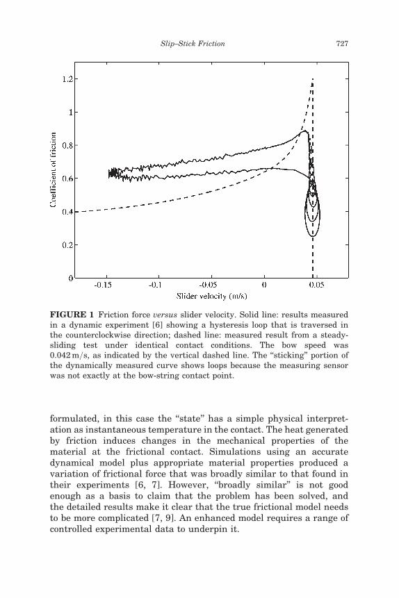
formulated, in this case the ‘‘state’’ has a simple physical interpret-ation as instantaneous temperature in the contact. The heat generatedby friction induces changes in the mechanical properties of thematerial at the frictional contact. Simulations using an accuratedynamical model plus appropriate material properties produced avariation of frictional force that was broadly similar to that found intheir experiments [6, 7]. However, ‘‘broadly similar’’ is not goodenough as a basis to claim that the problem has been solved, andthe detailed results make it clear that the true frictional model needsto be more complicated [7, 9]. An enhanced model requires a range ofcontrolled experimental data to underpin it.

FIGURE 1 Friction force versus slider velocity. Solid line: results measuredin a dynamic experiment [6] showing a hysteresis loop that is traversed inthe counterclockwise direction; dashed line: measured result from a steady-sliding test under identical contact conditions. The bow speed was0.042m=s, as indicated by the vertical dashed line. The ‘‘sticking’’ portion ofthe dynamically measured curve shows loops because the measuring sensorwas not exactly at the bow-string contact point.


Bowed-String Apparatus

We report here on experiments similar to references 6, 11, and 12, butemploying a system that shows a wider range of dynamical behaviorand that, thus, allows significantly different regions of parameterspace to be probed. Motivated by the considerable knowledge of thedynamics of bowed strings (e.g., references 14 and 15), we use a stringunder tension that is excited using a glass rod coated with the chosenfriction material, rosin for the results reported here. The basic appar-atus and method have been described previously [16]. A brief review isgiven to render this article self-contained, and then new extensions andresults are described: the major additions are a way to measure theaverage friction force, the use of additional regimes of oscillation, newresults deriving from an exploration of the effect of ambient tempera-ture, and the calculation of the energy flows during stick–slip vibration.

The glass rod is coated with commercial rosin of a type used for bassviolins. A homogeneous layer, with thickness on the order of microns,was applied by dissolving the rosin in xylene, and then immersingand withdrawing the rod at a constant velocity from the solution.The rod was allowed to dry for several days before being used. We havealso explored a dry application method, in which the rosin is applied ina powder form. The initial application resulted in a rather rough sur-face, with a friction force about twice as large as in the dipped method.However, after several passes of the rod on the string along the samewear track the friction forces became indistinguishable from those of asystem produced by the dipping method.

The apparatus is sketched in Figure 2. The rod is pressed againstthe string, which is mounted on a frame on micrometer mounts thatallow the normal force of the string on the rod to be adjusted. Therod is 250mm long and 6mm in diameter, mounted on an aluminumplate into which a semicircular groove has been machined. Electricheaters on the aluminum plate allow the rod to be heated. The rodand plate are moved by a constant velocity stage (Aerotech modelATS70030-U, Pittsburgh, PA, USA). In each run the carriage of thestage moves 0.2m at a constant speed 0.2m=s, with a peak-to-peakvariation of about 5%. Acceleration and deceleration both occupyabout 0.1 s, so all runs last slightly longer than 1 s. A violin E stringis used: it is a high-tensile steel monofilament with a diameter of270 mm and is stretched between two end supports 315mm apart.The tension in the string is adjusted so it oscillates at 650Hz, givingmany hundreds of periods of oscillation in each run. The resultsobtained are found to be independent of whether the string is cleanedbefore each run.


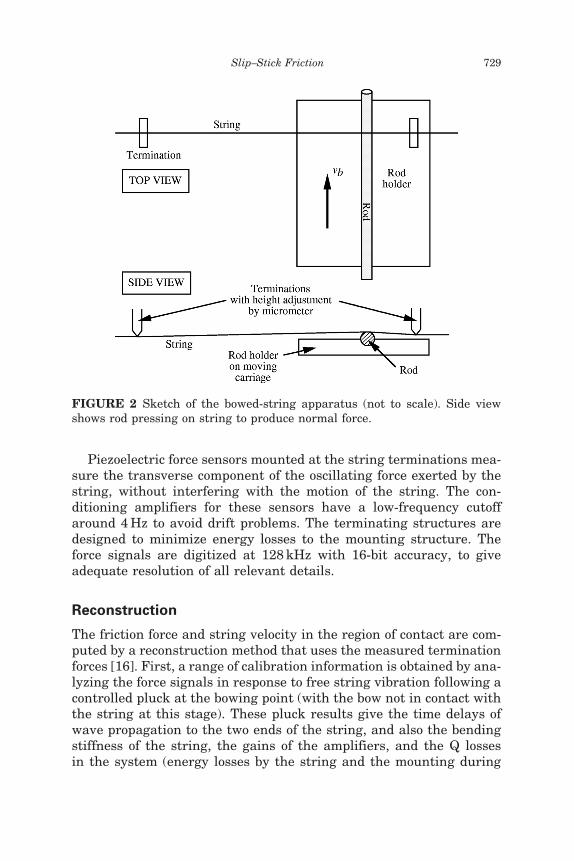
Piezoelectric force sensors mounted at the string terminations mea-sure the transverse component of the oscillating force exerted by thestring, without interfering with the motion of the string. The con-ditioning amplifiers for these sensors have a low-frequency cutoffaround 4Hz to avoid drift problems. The terminating structures aredesigned to minimize energy losses to the mounting structure. Theforce signals are digitized at 128 kHz with 16-bit accuracy, to giveadequate resolution of all relevant details.

Reconstruction

The friction force and string velocity in the region of contact are com-puted by a reconstruction method that uses the measured terminationforces [16]. First, a range of calibration information is obtained by ana-lyzing the force signals in response to free string vibration following acontrolled pluck at the bowing point (with the bow not in contact withthe string at this stage). These pluck results give the time delays ofwave propagation to the two ends of the string, and also the bendingstiffness of the string, the gains of the amplifiers, and the Q lossesin the system (energy losses by the string and the mounting during

FIGURE 2 Sketch of the bowed-string apparatus (not to scale). Side viewshows rod pressing on string to produce normal force.


vibration). The decay of each individual normal mode after the pluckcharacterizes Q losses: 2p=Qn is the fraction of energy in the nth modelost per cycle of its vibration. All string modes have Qn > 1000, someas high as 3000.

The reconstruction algorithm then combines the forces measured atthe two terminations, using the parameters from the pluck experi-ments, to calculate the velocity, v(t), of the center of the string, andthe friction force, F(t), at the bowing point. Each of these quantitiescan be calculated in two different ways, which provides a built-incheck on the accuracy of reconstruction.

Because the string makes contact with the rod at its periphery, thetime-varying friction force will also excite torsional motion of thestring. This means that the velocity of the string’s surface will besomewhat different from the reconstructed center velocity. Anexample showing very strong torsional motion was presented and ana-lyzed in reference 16. This case arose from a resonant interaction witha torsional string mode. For the results to be shown here, resonant tor-sional motion has been avoided; nevertheless, some torsion is inevi-tably present and this slightly complicates the interpretation ofresults, as is discussed later.

Measurement of the Average Frictional Forceand Normal Force

Because of the low-frequency roll-off of the measured force signals, thereconstruction of the dynamic friction force, F(t), from the measuredtermination forces can only give the AC component. To obtain theDC component of the frictional force, an optical method has beendeveloped. The DC frictional force, and also the normal force set bythe micrometers, can be deduced from the displacement of the stringat the point of contact with the rod. A force F, either in the plane ofthe string and the rod or in the direction normal to it, produces adeflection, d, conveniently expressed by

F ¼ 2Zd

Tbð1� bÞ þ bending stiffness correction ð1Þ

where T is the period of oscillation, b is the fractional distance of thecontact point to the nearer termination, and Z is the wave impedanceof the string given by Z ¼ 2M=T, where M is the total mass of thestring between the terminations. For the string used hereZ ¼ 0.17 kg=s. The bending stiffness correction turns out to be negligi-ble for this very thin string (although it plays an important role in thereconstruction of AC force [16]). The normal force, N, is determined


directly from Equation (1) from the displacement given by the micro-meters. For a 1 N force, the displacement of the string in these experi-ments is about 400 mm.

The lateral displacement caused by the average friction force duringoscillation is measured with a video microscope oriented normal to theplane of oscillation of the string. The images are recorded during eachrun: about 22 periods of oscillation occur per video frame. The averageposition of the blurred image of the string at the bowing point is thendetermined from each individual frame of the recording, displayedagainst a calibrated reticle. The mean displacement of the string asa result of the frictional force typically lies in the range 40–150 mmin these experiments. The measured displacement from each framethen produces the DC component of the frictional force, Fdc, fromEquation (1).

Advantages of the Bowed-String Method

The particular strengths of this new approach to friction characteriza-tion become apparent when the dynamics of bowed-string motion areexamined. There are three major features to note.

(1) In the earlier experiments, the apparatus was supposed to vibratewith only a single degree of freedom. However, all physical systemshave higher modes of vibration, and, because stick–slip motiongenerates forces with a wide frequency bandwidth, these highermodes make interpretation of results much more complicated.The stretched-string apparatus gets around this problem entirely:the string has many vibration modes, but they are all takeninto account in the reconstruction algorithm. This allows usefuldata to be collected over the full audio-frequency bandwidth.

(2) A stretched string excited by bowing exhibits a very rich range ofdynamical behavior, both periodic and nonperiodic. Different per-iodic regimes, transitions between these regimes, and nonperiodictransient behavior all yield data, which can shed light on manydifferent aspects of the underlying frictional constitutive law.We present results relating to three types of periodic motion,and also from an unusual transient event. Each of these typesof oscillation results in a characteristically different time-varyingvelocity and force on the friction point. Furthermore, the issue ofwhich oscillation regime the string chooses under given conditionsis a particularly challenging one for theoretical models, and, thus,these data provide a sensitive test. A friction model that couldpredict the correct sequence of oscillation regimes during this


kind of transient stick–slip test would have good claims to be con-vincing. At least for rosin, this is not an unrealistic objective: ithas been shown that a skilled violinist can control the lengthand nature of initial transients with impressive consistency [17],so the inherent variability of frictional interfaces cannot be usedas an excuse for poor models!

(3) The oscillation regime normally used by violinists is called theHelmholtz motion [18], and its form is quite counterintuitive. Atany given instant, the string forms a V shape with two virtuallystraight segments joined by a sharp corner. This corner travelsback and forth along the string, one round trip per period, tracingout the visible envelope of the string motion. As it passes the bowit triggers transitions between sticking and slipping friction, sothat the motion has one sticking period and one slipping periodper cycle. The timing is determined by the bowing position: inideal Helmholtz motion there is sticking for a time ð1� bÞT andslipping for the much shorter time bT every period. For ourexperiment, these times are approximately 1.35ms and 0.15ms,respectively. During sticking, the string moves at the speed, vb,of the bow (0.2m=s), whereas during slipping it moves at velocity�vbð1� bÞ=b, about �1.8m=s. Stick–slip motion based on a single-degree-of-freedom system behaves very differently: unless thenormal force is very high, the interval of sticking is very shortand the maximum slipping speed is approximately equal to thebowing speed (see, for example, reference 19). The result is thatthe bowed-string apparatus operates under a significantly differ-ent combination of force, speed, and timescale parameters and,therefore, yields data that can test theories in a different regime.

RESULTS AND DISCUSSION

Regimes of Oscillation

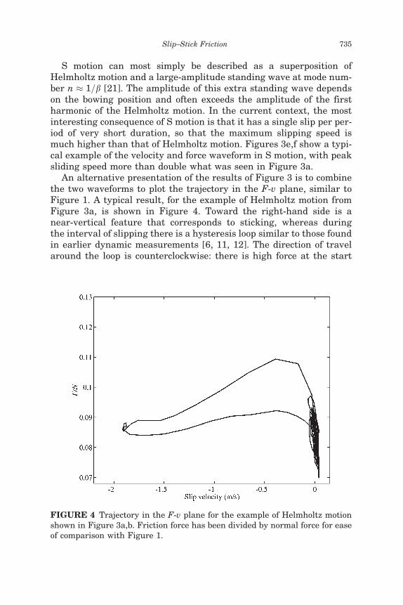
A typical example of the bowing-point velocity waveform for ourexperimental string during Helmholtz motion is shown in Figure 3a.The velocity axis is labeled in the coordinate system of the rod, so thatthe sticking velocity is zero. However, the measured velocity is notexactly zero for the sticking period: there are small-amplitude ripplesthat are discussed later. In Figure 3b we show the correspondingwaveform of friction force F(t). A striking feature of this plot is anegative one: the force waveform does not show any obvious distinc-tion between sticking and slipping, although this is the dominantfeature of the velocity waveform.


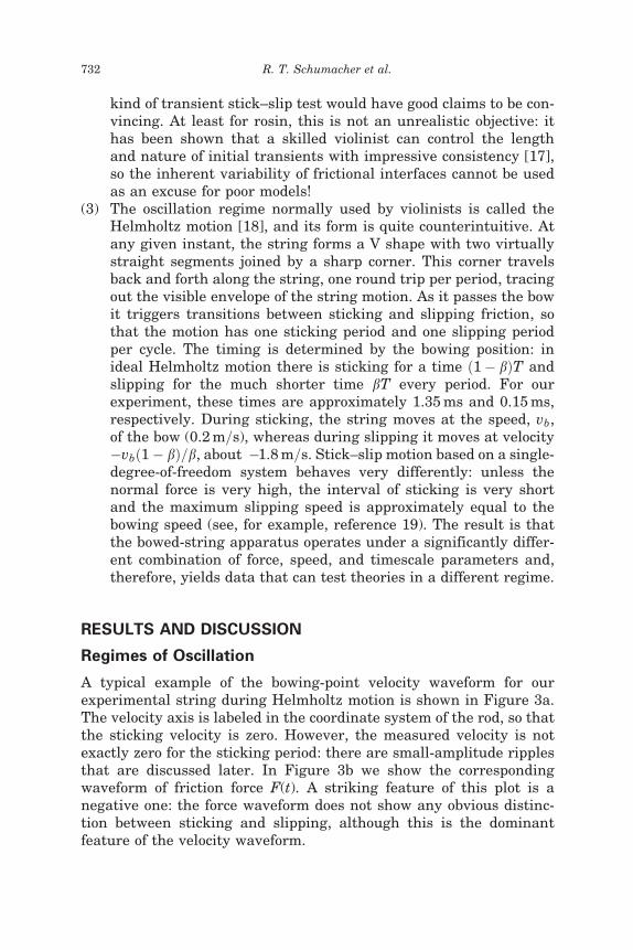
FIGURE 3 Waveforms of reconstructed velocity and force for three examplesof string motion; (a, b) Helmholtz motion, with normal force 2.5 N and meanfriction force 0.2 N; (c, d) double-slipping motion, with normal force 2.2 Nand mean friction force 0.29 N; and (e, f) S motion, with normal force 4.1 Nand mean friction force 0.4 N. Note the differing force and velocity scales.Measurements done at room temperature (22�C).


In addition to Helmholtz motion, results are shown for two othertypes of string motion from the classification first developed in afamous article by C. V. Raman [20] in 1918: a double-slip oscillationand a particular Raman ‘‘higher type’’ denoted S motion [21].Double-slip motion has two episodes of slipping per period, each ofapproximately the same duration as Helmholtz slips. It, therefore,has smaller slip velocity than in Helmholtz motion, because in anyperiodic motion the velocity of the string (in the reference frame ofthe fixture holding the string) must integrate to zero over a period.Animations of double-slipping motion and Helmholtz motion can befound in reference 22. Double-slipping motion is most often foundeither when the normal force is low [23] or during an initial transient.The smaller of the two slips then dies out as the string approaches itsstable oscillating state, usually Helmholtz motion. The velocity andforce waveforms for a typical example during such transient double-slipping motion are shown in Figures 3c,d: it is apparent that thisexample is not exactly periodic. However, the measurement methodmakes no assumption of periodic motion, so that it can produce usefulresults from all parts of a run.

FIGURE 3 Continued.


S motion can most simply be described as a superposition ofHelmholtz motion and a large-amplitude standing wave at mode num-ber n � 1=b [21]. The amplitude of this extra standing wave dependson the bowing position and often exceeds the amplitude of the firstharmonic of the Helmholtz motion. In the current context, the mostinteresting consequence of S motion is that it has a single slip per per-iod of very short duration, so that the maximum slipping speed ismuch higher than that of Helmholtz motion. Figures 3e,f show a typi-cal example of the velocity and force waveform in S motion, with peaksliding speed more than double what was seen in Figure 3a.

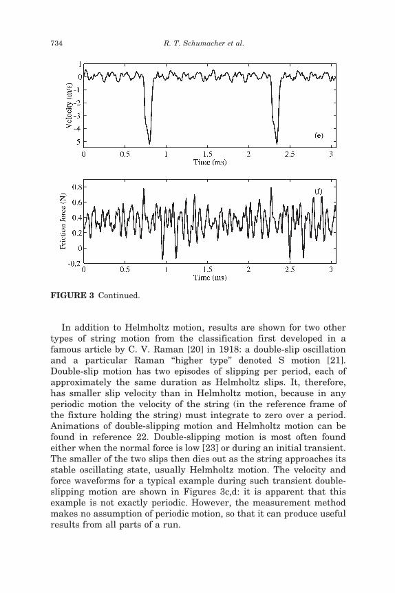
An alternative presentation of the results of Figure 3 is to combinethe two waveforms to plot the trajectory in the F-v plane, similar toFigure 1. A typical result, for the example of Helmholtz motion fromFigure 3a, is shown in Figure 4. Toward the right-hand side is anear-vertical feature that corresponds to sticking, whereas duringthe interval of slipping there is a hysteresis loop similar to those foundin earlier dynamic measurements [6, 11, 12]. The direction of travelaround the loop is counterclockwise: there is high force at the start

FIGURE 4 Trajectory in the F-v plane for the example of Helmholtz motionshown in Figure 3a,b. Friction force has been divided by normal force for easeof comparison with Figure 1.


of each slipping episode, reducing as the sliding speed increases, butnot increasing to the same high level when sliding slows down andsticking resumes.

Figure 4 has been plotted with the friction force scaled by the nor-mal force, so that the results can be compared quantitatively withFigure 1. It is immediately apparent that the values are much smallerin Figure 4, even though the friction material is essentially the same.The difference comes from the contact conditions. The axis in Figure 4is deliberately not labeled ‘‘coefficient of friction’’ because this experi-ment is not operating in the familiar Coulomb friction regime in whichthe ratio F=N is constant. As is demonstrated in a later section, thecontact conditions are such that one would expect it to be operatingin the Hertzian contact regime for which in the ideal case frictionforce, F, would be proportional to N2=3, so the ratio F=N would be pro-portional to N�1=3 (see, for example, Johnson [24]). In other words, thecontact has the nature of a large single asperity, not of a rough surfacewith multiple contacting asperities. With a smaller normal load, thevalue of F=N would be expected to rise from the low value seen inFigure 4, and this is the most likely explanation of the discrepancywith Figure 1: the experiment that generated Figure 1 used differentcontact geometry, leading to reduced contact pressure and, thus, tohigher friction force.

As an aside, this observation about contact regime and typical fric-tion force may explain why a violin string is normally bowed using arosin-coated ribbon consisting of many separate strands of horsehair,rather than with a rod as in these tests. A friction force as low as onetenth of the normal force would make life difficult for a violinist. Theribbon of hairs in a conventional bow produces multiple contacts thatwill behave much like multiple asperities. This increases the real areaof contact and, thus, gives a larger friction force that is more nearlylinear with normal force over the range relevant in practice.

Sticking, Creep, and the Effect of Temperature

A universal feature of all F-v plots from this apparatus is that the velo-city of the string at the bowing point never lingers exactly at zero dur-ing ‘sticking,’ as one might expect. Instead, a patch of ‘‘scribble’’ isseen, as in the lower right section of Figure 4. In the region wherethe friction force is highest, a curve is seen rather than a clear-cuttransition that would allow one to define exactly when sticking stopsand slipping begins. (The curve appears angular in the plot becausethe transition through this range is so fast that individual digitalsamples are seen, even with a sampling rate of 128kHz. Such rapid


transitions are another unusual feature of this friction-measuringapparatus.) The maximum frictional force occurs when there is verysignificant relative motion between rod and string, at a rate of some0.4m=s for the case shown. The F-v plot is a useful way to examinethe question ‘‘what, if anything, is sticking?’’ As is explained shortly,the detailed shape of the trajectory gives important clues about theassociated physical processes.

There are two different types of process in operation when scribbleis generated. First, as has already been pointed out, the friction forcewill generate some torsional motion of the string, which could giverise to rolling without violating the condition of sticking. The velocityreconstructed by this measurement method is of the center of thestring (and also, therefore, of the center point of the contact regionbetween string and rod). Rolling would show up in the waveformof center velocity, but in the context of F-v plots it would generate‘scribble,’ which was simply an artifact, because F was being plottedagainst the ‘‘wrong’’ v. Because there can be no long-term cumulativerolling motion, this effect tends to produce scribble which is onaverage centered on the true sticking speed (zero in this referenceframe).

However, although rolling undoubtedly accounts for some of theobserved ‘‘sticking scribble,’’ it is not the whole story. These experi-ments also show systematic deviations of the center of the scribbleaway from zero velocity, strongly suggesting that there is some genu-ine relative movement between the surface of the string and the glasscore of the rod during the intervals of nominal sticking. In otherwords, the state commonly described as sticking is rather more elusivethan the word suggests, with some deformation taking place in therosin layer.

A series of measurements has been carried out in which theambient temperature around the rod and friction-contact zone wassystematically changed, and this gives the clearest evidence for defor-mation in the rosin layer during sticking. The results shown inFigures 3 and 4 were obtained with ambient temperature around22�C. When temperature was raised sufficiently, to around 60�C,self-excited vibration of the string was found to cease entirely, givingthe first direct proof that temperature plays a role in the mechanics of‘stick–slip’ friction mediated by rosin, as had been proposed previouslyon the basis of less-direct evidence [6, 7]. The most interestingbehavior was seen at a temperature just a little lower, around 56�C.At this temperature the string remained almost stationary for the firsthalf of the run, but then oscillation grew from small amplitude until,after some tens of period lengths, it settled into fairly normal-looking


Helmholtz motion. Figure 5 shows the F-v plot from the fully developedHelmholtz motion.

Figures 4 and 5 show significantly different shapes and sizes ofloop during slipping, but more relevant for the present discussion isa difference of detailed shape in the sticking portions of the curves.Figure 5 shows some scribble, but it also shows a very clear systematiceffect in which the curve through the middle of the scribble bends con-spicuously toward the left at high friction force. Indeed, detailedinspection of the data of Figure 5 reveals a clear correlation betweenF and v throughout the sticking portion, each loop within the scribblehaving a definite tilt. A similar trend is found, rather less obviously,within the band of scribble in Figure 4.

The data from the ‘‘hot’’ run is even more striking when thetransient part of the motion is examined. Figure 6a shows the velocitywaveform during the growth phase of the oscillation. The waveformlooks very much like the Helmholtz slip–stick pattern across the wholeof this plot, but the ‘sticking’ speed (the plateau level near the top ofthe plot) is not constant, and on the left of the plot it is well below zero

FIGURE 5 Trajectory in the F-v plane for Helmholtz motion at elevated rodtemperature of 56�C. The normal force is 4.1 N, and the mean friction force is0.4 N. Friction force has been divided by normal force for ease of comparisonwith Figures 1 and 4. Scales are the same as Figure 4.


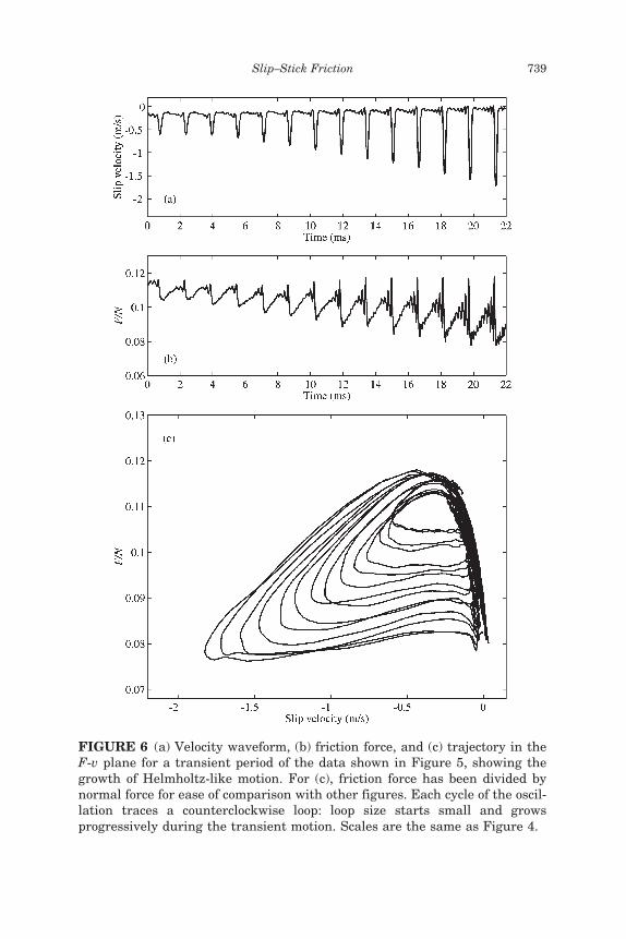
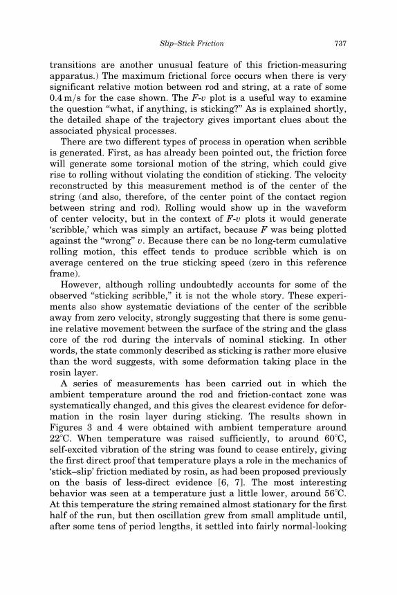
FIGURE 6 (a) Velocity waveform, (b) friction force, and (c) trajectory in theF-v plane for a transient period of the data shown in Figure 5, showing thegrowth of Helmholtz-like motion. For (c), friction force has been divided bynormal force for ease of comparison with other figures. Each cycle of the oscil-lation traces a counterclockwise loop: loop size starts small and growsprogressively during the transient motion. Scales are the same as Figure 4.


(the speed of the rod). How can there be sticking under thoseconditions? This counterintuitive pattern becomes more understand-able when the friction-force plot is examined, as shown in Figure 6b.During the growth of the oscillation the mean value of friction forcefalls by a significant factor: before the oscillation started, the meanfriction force was about 0.5 N, and by the time the Helmholtz motionis fully established, this has fallen by 20% to 0.4 N.

When the velocity and force data are put together into the F-v plot,as in Figure 6c, an outward-spiraling series of loops is traced out bysuccessive cycles, but these all have their sticking portions lyingon essentially the same curve. The small loops, associated with theearlier part of the transient growth, have sticking speeds that aresignificantly negative, as was seen in Figure 6a. However, this vari-ation in ‘sticking’ speed can now be seen to be correlated with thedecrease in DC frictional force, following essentially the same tiltingcurve identified in Figure 5 from the fully developed Helmholtzmotion.

It must be admitted that this observation of a common backbonecurve during ‘sticking’ is somewhat speculative, because of uncertain-ties arising from the inherent errors associated with the video analysisfor measuring the DC force. A skeptical reader may question whetherthe evidence of Figures 5 and 6 is clear enough to be compelling. Theproblem is that the transient examined here occupies a total time thatis less than one frame of the video analysis, so that the method canonly yield a rather coarse and approximate version of the DC forceduring a transient like this, based on interpolation between relativelysparse neighboring data points. More and better data need to be gath-ered to test the interpretation suggested here, but, nevertheless, theseresults give an intriguing clue about a possible physical model ofthe processes taking place within the rosin layer, which is worthcomment.

A possible interpretation of these results is to suggest that the‘sticking’ periods involve some kind of viscous flow in the rosin layer,with a shear force strongly correlated with velocity or shear strainrate. It would be natural to call this viscous flow ‘‘creep,’’ except thatit should be noted that with the speed and layer thickness relevanthere, the strain rate is of the order of 105 s�1. This enormous strainrate is by no means what would usually be called creep, and indeedit rivals the highest strain rates that can be obtained in measurementrigs involving projectiles and shock-wave generation!

The slope of the curve in Figure 6c can be used (together with infor-mation about the contact size) to deduce an effective creep viscosity.The shape of the curve then clearly indicates a nonlinear relation


between viscosity and shear rate (a relation that also varies withambient temperature). Crucially, there appears to be some kind ofsoftening behavior in which the shear viscosity (i.e., the slope of thecurve) is lower when the shear rate is higher. But softeningbehavior of this general kind is well known to lead to instabilityinvolving the formation of a localized shear band, as has been observedin a range of different materials and systems (see, for example, refer-ences 25 and 26). Could an instability of this kind give a basis for atransition between two states, which we might label ‘‘sticking withcreep’’ and ‘‘gross sliding?’’

The speculative model might run as follows. When the shear stressor strain reaches a critical level, softening behavior (linked to tem-perature rise [26]) would lead to the formation of an unstable localizedshear band somewhere within the thickness of the rosin layer. Whenthe instability takes hold, there would be a short period during whichthe pattern of deformation adjusts to become concentrated in the shearband: this would correlate with the rounded peak seen in all the F-vplots surrounding the maximum friction force, where, as already com-mented, the change is so rapid that individual digital samples are seenin the plots.

There would then follow an episode of gross sliding during whichthe deformation was largely confined to a very thin interfacial layer,with consequent large temperature changes [6, 7]. During such grosssliding there is no clear evidence that sliding velocity is a major con-trolling variable, and a model involving a temperature-dependentinterfacial shear strength as presented by Smith and Woodhouse [6]may be appropriate. Gross sliding would come to an end when the kin-ematics of the string motion led to the total shear-strain rate droppingback to a value near zero, so that the shear band might ‘‘heal’’ and‘‘sticking with creep’’ resume.

This picture seems to be consistent with all the major features of theresults presented here, and also to have the potential to resolve anunsatisfactory conflict between two models for rosin friction proposedearlier [6]: a ‘viscous model’ and a ‘plastic yield model,’ both of whichwere shown to have promising features. Under this new picture, boththose models could be relevant, applying in different parts of themotion as a shear band forms and heals within the rosin layer at a fre-quency of hundreds of Hertz. To explore these ideas further requiresnew modeling and simulation and is a goal for future work. The modelcould possibly be relevant not only to rosin but also to other visco-elastic materials or non-Newtonian fluids for which experiments havesuggested some kind of ‘‘yield fluid’’ constitutive law (see, for example,reference 27).


Wear Tracks and Contact Size

Further evidence that bears upon the question of what happens dur-ing sticking can come from an examination of the wear tracks left inthe rosin coating on the rod after a single pass over the vibratingstring. A typical SEM micrograph is shown in Figure 7a. This micro-graph is reproduced from reference 16 (Figure 8a). It is not from thesame run as any of the earlier figures shown here, but it is chosenbecause it illustrates a variety of interesting features in a single pic-ture. For this particular oscillation regime, there were two slips perperiod with a very brief sticking interval between. That accounts forthe alternating pattern of the sticking scars. The regions marked Aand B are the undisturbed surface of the rosin coating. The scarsbelow letters A were created during the longer of the two stickingperiods in each cycle of the string motion, and those below B duringthe shorter sticking periods. The wider spreads (horizontal in thefigure) of the scars under A compared to those under B reflects this dif-ference of sticking time: longer sticking means that more contactmovement, whether rolling or creeping, can occur. Debris has beenprojected some distance from the track. The regions marked C are slip-ping tracks. D marks an area of adhesive failure, where the rosin haseither been removed entirely from the glass surface, or has left only avery thin layer behind.

In Figure 7b (an enlargement of part of Figure 7a), the region ofadhesive failure is more clear. E marks debris created possibly bycohesive failure, F marks fracture cracks on a piece of debris, and Gshows a region with a texture highly suggestive of the phenomenonknown as the ‘‘printer’s’’ or ‘‘ribbing’’ instability: see, for example,reference 28. Thus, the rosin shows both brittle fracture characteristicof a glass and viscous flow characteristic of a fluid. This mixture ofbehaviors in such close proximity is strongly suggestive of tempera-ture-induced material changes.

To relate these wear tracks to the information obtained from thefriction-force reconstruction it is useful to plot the force results in a dif-ferent way. By integrating the velocity signal, friction force can beplotted as a function of distance, x, along the rod surface. Note thatin this case there is no uncertainty resulting from torsional motionof the string; the reconstructed velocity corresponds precisely to themotion of the center of the contact patch between rod and string.Figure 8a shows F(x) for two typical cycles during the Helmholtzmotion of Figure 3a.

Figure 8b shows an enlarged view of the center sticking region ofFigure 8a. Unfortunately, there is some uncertainty in this region


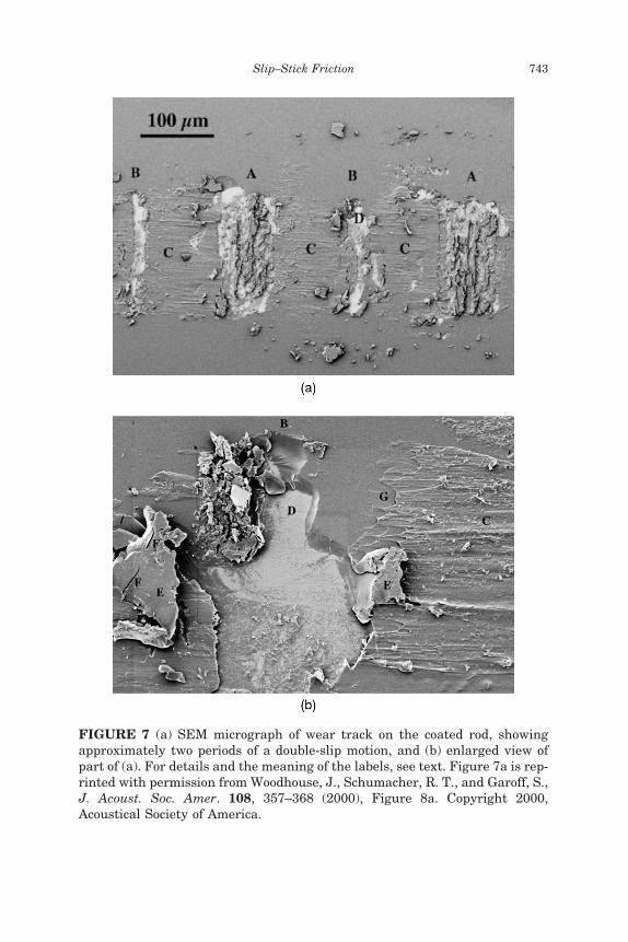
FIGURE 7 (a) SEM micrograph of wear track on the coated rod, showingapproximately two periods of a double-slip motion, and (b) enlarged view ofpart of (a). For details and the meaning of the labels, see text. Figure 7a is rep-rinted with permission from Woodhouse, J., Schumacher, R. T., and Garoff, S.,J. Acoust. Soc. Amer. 108, 357–368 (2000), Figure 8a. Copyright 2000,Acoustical Society of America.


FIGURE 8 (a) Friction force as a function of position along the surface of therod, for the Helmholtz motion of Figure 3a, and (b) magnification of one stick-ing episode of (a).


because the instantaneous rod velocity is perturbed by small-amplitude oscillations of the moving carriage drive system. To plotthis version of the figure, a value has been chosen for the rod velo-city, within the known error bounds, which minimizes the lateralextent of the motion during sticking. This may mean that cumulativedrift resulting from creep has been removed. Despite this uncer-tainty, some features visible here are clearly characteristic of thesticking of the string to the rod. Complex motion of the center ofthe string during sticking is evident, although whether this arisesfrom rolling, creep, or a mixture of both cannot be resolved from thisevidence alone.

The extent of movement of the sticking region revealedby Figure 8b is only some 3 mm, much less than the physical sizeof the sticking scars seen in the micrographs. Part of the reasonmay be missing cumulative creep, as just mentioned, but it mustalso be remembered that the physical scar corresponds, more orless, to the entire region over which there was some contactbetween the rod and the surface of the string during the stickinginterval. The size of this region is influenced not only by movementof the center of the contact, but also by effects of local deformationcaused by the contact forces. Even if effects resulting from the rela-tively soft rosin layer are ignored, we have contact between twocrossed cylinders of glass and steel. The form of local deformationunder such conditions is well known, from the classical work ofHertz (see, for example, Johnson [24], Chapter 4). The contact zoneis an ellipse with dimensions determined by the radii of the twocylinders and their respective Young’s moduli of elasticity. Carryingthe calculation through with appropriate parameter values for thestring and the glass rod yields a contact region that for a normalforce of 4N has approximate dimensions 160� 20 mm, which is ofthe same order as the typical dimensions of the narrowest observedsticking scars.

From the same Hertz contact calculation, it is also straightforwardto calculate the contact-pressure distribution: the average pressure fora normal force of 4 N is 1.5GPa, with a distribution over the contactzone that rises from zero around the edge to a peak value above2GPa at the center. These pressures are enormous compared withany reasonable estimate for the compressive yield stress of a substancelike rosin, and this serves to justify a comment made earlier. Withpressures this high, any asperities resulting from surface roughnessof the glass rod, rosin coating, or the steel string are irrelevant becausethe rosin layer yields locally, leading to fully conforming contact overmost the Hertzian ellipse.


Energy Dissipation

A final topic of interest is the energy balance involved in frictionallyexcited oscillation. The energy flowing from the string to the rod(considered positive here) is

EðtÞ ¼ �Z t

0

vðsÞ � vb½ � FðsÞ þ Fdc½ �ds ð2Þ

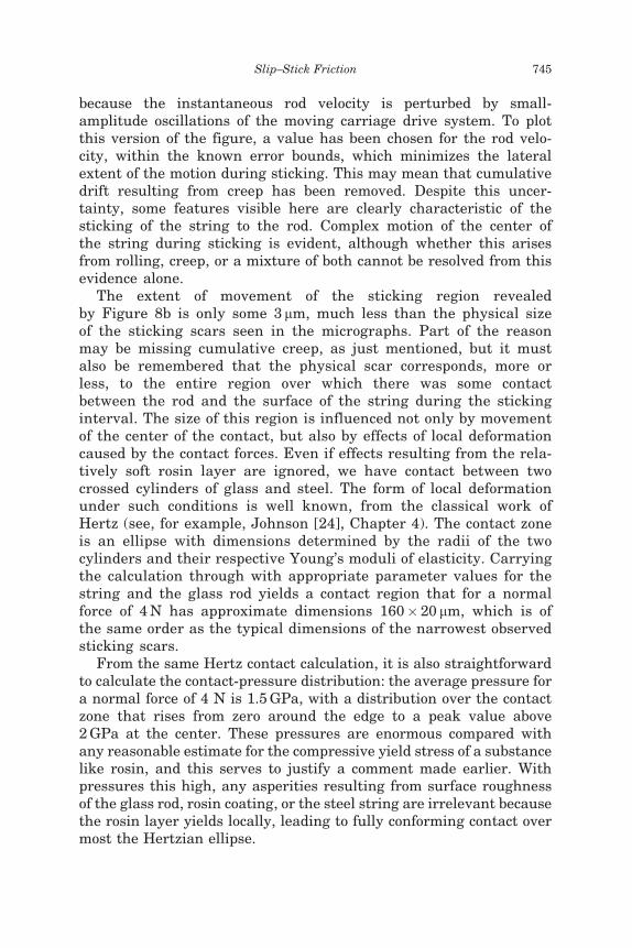
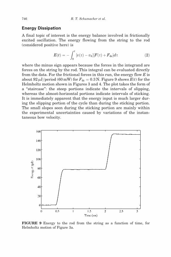
where the minus sign appears because the forces in the integrand areforces on the string by the rod. This integral can be evaluated directlyfrom the data. For the frictional forces in this run, the energy flow E isabout 92mJ=period (60mW) for Fdc ¼ 0:3N. Figure 9 shows E(t) for theHelmholtz motion shown in Figures 3 and 4. The plot takes the form ofa ‘‘staircase’’: the steep portions indicate the intervals of slipping,whereas the almost-horizontal portions indicate intervals of sticking.It is immediately apparent that the energy input is much larger dur-ing the slipping portion of the cycle than during the sticking portion.The small slopes seen during the sticking portion are mainly withinthe experimental uncertainties caused by variations of the instan-taneous bow velocity.

FIGURE 9 Energy to the rod from the string as a function of time, forHelmholtz motion of Figure 3a.


During steady periodic motion of the string there is no change in thesum of kinetic and potential energies, and the energy flowing acrossthe frictional interface is all dissipated somewhere in the system. Thisenergy dissipation can be separated into four channels:

E ¼ Estring þ Erig þ cDAþ Elayer: ð3Þ

Estring is the energy loss into the string vibration, associated with thedissipation at the string’s terminations, by air resistance, and so on: inother words, it is the energy required to maintain the string oscillationwhen the rod is not in contact with the string. Erig is the correspondingenergy loss into the rig on the other side of the contact region: the rod,trolley, and so on. The term cDA is the energy needed to create thenew surface area, where c is the surface energy of the rosin layerand DA is the newly created area of the rosin=air interface. We defineElayer to be the energy required to reshape and move the rosinmaterial, as shown in the wear track of Figure 7.

It is straightforward to estimate the energy dissipated into the firstthree loss channels. Estring is deduced from the measured Q factors ofthe normal modes from the pluck results. By using the Fourierdecomposition of ideal Helmholtz motion (Helmholtz [18], AppendixVI) these Qs can be combined to give a total energy-loss rate from freevibration. We have included in this calculation all string modes up to20 kHz, which will give a slight overestimate of the actual energy lossbecause higher modes will be excited less strongly in practice than inthe ideal case. The result is Estring� 2.3 nJ=period (�1.5 mW), severalorders of magnitude smaller than the total energy transfer measuredpreviously. (This disparity of magnitudes was noted, in less detailedform, by Cremer [29], Section 3.6.) The corresponding term Erig is lesseasy to determine quantitatively, but the vibration modes of the righave Q factors that are in general lower than those of the string; themass of the rig is much higher than the string, and its modal densityis lower, so one can confidently predict that Erig will be at most of thesame order of magnitude as Estring.

We can also estimate the energy lost in creating new surface area.We assume c is on the order of 0.06 J=m2 (a number typical of a polarorganic material such as rosin [13]) and DA � 0:036� 10�6 m2=periodas estimated from the wear track. We then find that this loss channelis about 2.2 nJ=period (�1.5 mW). Thus, this channel is also a negli-gible fraction of the energy used in the system. We are left with thefact that Elayer, energy used to disrupt the rosin layer, accounts foralmost all energy dissipation in the system. Furthermore, virtuallyall of that energy is dissipated during the slipping portion of theoscillation.


DISCUSSION AND CONCLUSIONS

We have described an experimental approach to the characterizationof dynamic friction force using an apparatus based on a stretchedstring excited by a ‘‘bow’’ consisting of a glass rod coated with thedesired friction material, rosin for the results shown here. Stick–sliposcillations of the string are excited by moving the rod with a knownvelocity, and the friction force and the string velocity at the point ofcontact with the rod are inferred by processing of the signals from non-intrusive force transducers at the two ends of the string. We arguethat an inverse measurement of this general kind is the best way togather reliable data on the behavior of interfacial friction in thishigh-frequency dynamic regime, which is important to many engineer-ing applications.

The bowed string is a good system to use for this purpose, because itis well understood compared with other systems that exhibit friction-ally excited vibration. It offers several advantages compared with thesingle-degree-of-freedom systems that have been used in the past. Allthe modes of the string are taken into account in the processing, sothat there is no problem associated with unwanted higher modes ofthe apparatus. This greatly extends the useful frequency bandwidthof data. Another advantage of the bowed string is that it operates ina regime that falls in a different region of the parameter space relatingto contact conditions (normal force, sliding speed, rate of change ofsliding speed, etc.). This means that it can gather data complementaryto other methods. Finally, the string exhibits very rich dynamicalbehavior, showing a range of different characteristics. The methodused here makes no assumptions about the form of motion, so it canprovide useful data from different regimes of periodic motion, fromtransitions between such regimes, and from nonperiodic motion dur-ing initial transients or extended spells of chaotic motion. These datathrow down a gauntlet to the modelers to develop a frictional consti-tutive model that can reproduce quantitatively the rich range ofbehavior revealed.

The results of the friction-force measurement can be correlated withmicroscopic examination of the wear track left on the surface of the rodafter a single pass over the string. This gives additional insight intothe physical processes governing the friction force. These processeshave been shown to be complicated. The wear tracks exhibit a widerange of different features: brittle fracture, ductile failure, viscousflow, and the generation of and interaction with wear debris.

The results shown here, and others published previously using thesame friction material [6, 7, 9], demonstrate that dynamic friction in


this system is not fully captured by any of the friction models so farproposed. It has been directly confirmed that temperature plays asignificant role for this friction material. At sufficiently high ambienttemperature, stick–slip motion ceases entirely. Data have been shownat a temperature when self-excited vibration becomes marginally poss-ible, and the results compared with those at lower temperature whenstick–slip motion is ubiquitous.

Strong evidence has been shown for temperature-dependent shearflow in the rosin layer during sticking. It has been suggested that anonlinear viscous model might be a promising candidate to accountfor the observations, and that the transition to slipping might arisefrom an instability, perhaps associated with material softening, lead-ing to the formation of a shear band [25, 26]. During slipping, it hasbeen shown that a different type of governing law is needed for thefriction force, because sliding velocity is not strongly correlated withforce. Temperature within a thin interfacial layer is a strong candidate.

These results and conclusions suggest a range of further researchthat may be fruitful to advance understanding of the initiation andwaveforms of frictionally excited vibration. A variety of further experi-ments could be valuable, using the test rig described here. More andbetter data are needed on the effects of ambient temperature to testthe speculations advanced here. The friction material, normal force,sliding speed, and vibration frequency could all be varied with advan-tage. More careful analysis is needed of the regime of oscillationchosen by the string under different conditions. All this informationthen needs to be compared with simulation studies similar to thosealready reported by Woodhouse [7]. Simulation offers the most directroute to explore alternative constitutive laws for friction, such as theone proposed here. Rational design strategies to control stick–slipvibration in practical situations might then become possible.

ACKNOWLEDGMENTS

The authors thank K. L. Johnson, J. A. Williams and C. Y. Barlowfor helpful discussions on this research.

REFERENCES

[1] Akay, A., The acoustics of friction, J. Acoust. Soc. Amer. 111, 1525–1548 (2002).[2] Johnson, K. L., Dynamic friction, in Tribology Research: From Model Experiment to

Industrial Problem, G. Dalmaz, A. A. Lubrecht, D. Dowson, and M. Priest (Eds.)(Elsevier Science, Amsterdam, 2001), pp. 37–45.

[3] Urbakh, M., Klafter, J., Gourdon, D., and Israelachvili, I., The nonlinear nature offriction, Nature 430, 525–528 (2004).


[4] Ruina, A., Slip instability and state variable laws, J. Geophys. Research 88, 10359–10370 (1983).

[5] Heslot, F., Baumberger, T., Perrin, B., Caroli, B., and Caroli, C., Creep, stick–slip,and dry-friction dynamics: Experiments and a heuristic model, Phys. Review E 49,4973–4988 (1994).

[6] Smith, J. H. and Woodhouse, J., The tribology of rosin, J. Mech. Phys. Solids 48,1633–1681 (2000).

[7] Woodhouse, J., Bowed string simulation using a thermal friction model, Acustica—Acta Acustica 89, 355–368 (2003).

[8] Duffour, P., Noise generation in vehicle brakes, Doctoral thesis, University ofCambridge, UK (2002).

[9] Galluzzo, P. M., On the playability of stringed instruments, Doctoral thesis,University of Cambridge, UK (2003).

[10] Mills, K., ASM Handbook: Fractography V. 12 (ASM International, Metals Park,OH, 1991).

[11] Bell, R. and Burdekin, M., A study of the stick–slip motion of machine tool feeddrives, Proc. Inst. Mech. Engrs. 184, 543–560 (1969–70).

[12] Brockley, C. A. and Ko, P. L., Quasi-harmonic friction-induced vibration, Trans.ASME J. Lub. Tech. 92, 550–556 (1970).

[13] The Merck Index, 9th edition, M. Windholz, S. Budavari, L. Stroumtsos, andM. Fertig (Eds.) (Merck & Co., Rahway, NJ, 1976), p. 1071.

[14] Schumacher, R. T. and Woodhouse, J., The transient behavior of models of bowed-string motion, Chaos 5, 509–523 (1995).

[15] Woodhouse, J. and Galluzzo, P. M., The bowed string as we know it today,Acustica—Acta Acustica 90, 579–589 (2004).

[16] Woodhouse, J., Schumacher, R. T., and Garoff, S., Reconstruction of bowing pointfriction force in a bowed string, J. Acoust. Soc. Amer. 108, 357–368 (2000).

[17] Guettler, K. and Askenfelt, A., Acceptance limits for the duration of pre-Helmholtztransients in bowed string attacks, J. Acoust. Soc. Amer. 101, 2903–2913 (1997).

[18] Helmholtz, H. von, Lehre von den Tonempfindungen (Braunschweig 1862); Englishedition: On the sensations of tone (Dover, New York, 1954).

[19] Den Hartog, J. P., Forced vibration with combined Coulomb and viscous friction,Applied Mech. 53, 107–115 (1933).

[20] Raman, C. V., On the mechanical theory of vibrations of bowed strings, IndianAssoc. Cult. Sci. Bull. 15, 1–158 (1918).

[21] Lawergren, B., On the motion of bowed violin strings, Acustica 44, 194–206 (1980).[22] Woodhouse, J. and Galluzzo, P. M., Why is the violin so hard to play? Plus

31 October 2004, http:==plus.maths.org=issue31=features=woodhouse=index.html(online magazine of the Millennium Mathematics Project).

[23] Schelleng, J. C., The bowed string and the player, J. Acoust. Soc. Amer. 53, 26–41(1973).

[24] Johnson, K. L., Contact Mechanics (Cambridge University Press, Cambridge, UK1985).

[25] Bai, Y. L. and Dodd, B., Adiabatic Shear Localization (Pergamon, Oxford, 1985).[26] Swallowe, G. M. (Ed.), Mechanical Properties and Testing of Polymers (Kluwer

Academic, Dordrecht, 1999), Chapters 3, 4.[27] Bingham, E. C., Fluidity and Plasticity (McGraw-Hill, New York, 1922).[28] Lopez, F. V., Pauchard, L., Rosen, M., and Rabaud, M., Non-Newtonian effects on

ribbing instability threshold, J. Non-Newtonian Fluid Mech. 103, 123–139 (2002).[29] Cremer, L., The Physics of the Violin (MIT Press, Cambridge, MA, 1985).


probing the physics of slip–stick friction using a …jw12/jw pdfs/schumacher_garoff2.pdf · the...

Documents