Probably Approximately Correct Learning (PAC)

Leslie G. Valiant. A Theory of the Learnable.

Comm. ACM (1984) 1134-1142

Recall: Bayesian learning

• Create a model based on some parameters

• Assume some prior distribution on those parameters

• Learning problem– Adjust the model parameters so as to

maximize the likelihood of the model given the data

– Utilize Bayesian formula for that.

PAC Learning

• Given distribution D of observables X • Given a family of functions (concepts)

F• For each x ε X and f ε F:

f(x) provides the label for x

• Given a family of hypotheses H, seek a hypothesis h such thatError(h) = Prx ε D[f(x) ≠ h(x)]

is minimal

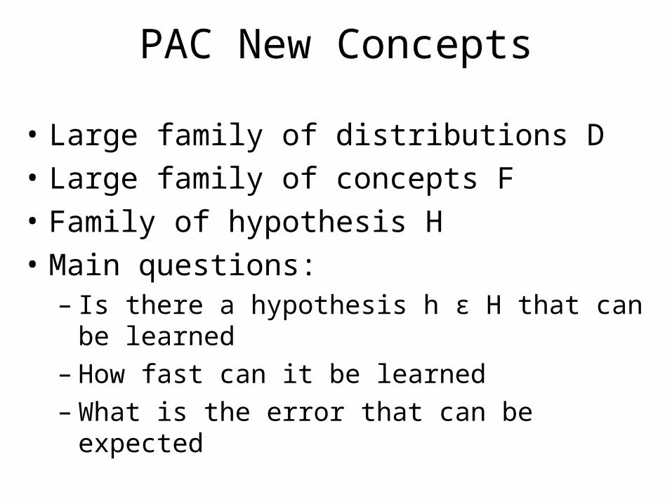
PAC New Concepts

• Large family of distributions D• Large family of concepts F• Family of hypothesis H• Main questions:

– Is there a hypothesis h ε H that can be learned

– How fast can it be learned– What is the error that can be expected

Estimation vs. approximation

• Note:– The distribution D is fixed– There is no noise in the system

(currently)– F is a space of binary functions

(concepts)

• This is thus an approximation problem as the function is given exactly for each x X

• Estimation problem: f is not given exactly but estimated from noisy data

Example (PAC)

• Concept: Average body-size person• Inputs: for each person:

– height– weight

• Sample: labeled examples of persons– label + : average body-size– label - : not average body-size

• Two dimensional inputs

Observable space X with concept f

Example (PAC)

• Assumption: target concept is a rectangle.

• Goal:– Find a rectangle h that

“approximates” the target– Hypothesis family H of rectangles

• Formally:– With high probability– output a rectangle such that– its error is low.

Example (Modeling)

• Assume:– Fixed distribution over persons.

• Goal: – Low error with respect to THIS

distribution!!!• How does the distribution look

like?– Highly complex.– Each parameter is not uniform.– Highly correlated.

Model Based approach

• First try to model the distribution.• Given a model of the distribution:

– find an optimal decision rule.

• Bayesian Learning

PAC approach

• Assume that the distribution is fixed.

• Samples are drawn are i.i.d.– independent

– Identically distributed

• Concentrate on the decision rule rather than distribution.

PAC Learning

• Task: learn a rectangle from examples.

• Input: point (x,f(x)) and classification + or -– classifies by a rectangle R

• Goal: – Using the fewest examples

– compute h

– h is a good approximation for f

PAC Learning: Accuracy

• Testing the accuracy of a hypothesis:– using the distribution D of examples.

• Error = h f (symmetric difference)

• Pr[Error] = D(Error) = D(h h)

• We would like Pr[Error] to be controllable.

• Given a parameter : – Find h such that Pr[Error] <

PAC Learning: Hypothesis

• Which Rectangle should we choose?– Similar to parametric modeling?

Setting up the Analysis:

• Choose smallest rectangle.

• Need to show:– For any distribution D and Rectangle h

– input parameters: and– Select m() examples

– Let h be the smallest consistent rectangle.

– Such that with probability 1-(on X):

D(f h) <

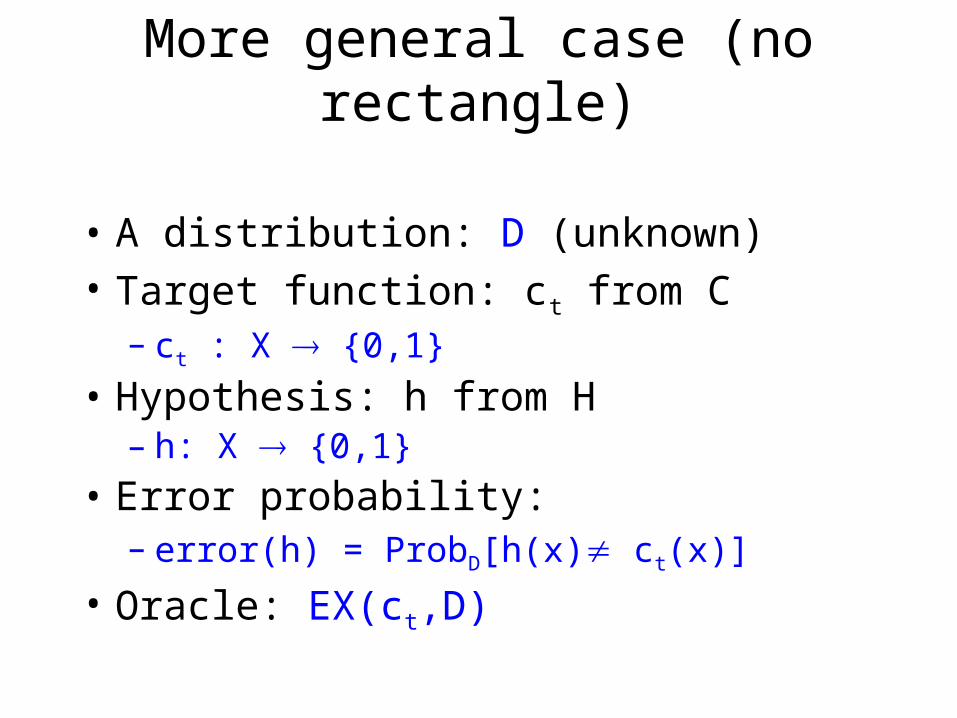
More general case (no rectangle)

• A distribution: D (unknown)• Target function: ct from C

– ct : X {0,1}

• Hypothesis: h from H– h: X {0,1}

• Error probability:– error(h) = ProbD[h(x) ct(x)]

• Oracle: EX(ct,D)

PAC Learning: Definition

• C and H are concept classes over X.• C is PAC learnable by H if• There Exist an Algorithm A such that:

– For any distribution D over X and ct in C– for every input and :– outputs a hypothesis h in H,– while having access to EX(ct,D)– with probability 1-we have error(h) <

• Complexities.

Finite Concept class

• Assume C=H and finite.• h is -bad if error(h)> .• Algorithm:

– Sample a set S of m(,) examples.– Find h in H which is consistent.

• Algorithm fails if h is -bad.

• X is the set of all possible examples• D is the distribution from which the

examples are drawn• H is the set of all possible hypotheses,

cH• m is the number of training examples• error(h) =

Pr(h(x) c(x) | x is drawn from X with D)

• h is approximately correct if error(h)

PAC learning: formalization (1)

PAC learning: formalization (2)

To show: after m examples, with high probability, all consistent hypotheses are approximately correct.

All consistent hypotheses lie in an -ball around c.

cHbadH

Complexity analysis (1)

• The probability that hypothesis hbadHbad

is consistent with the first m examples:

error(hbad) > by definition.

The probability that it agrees with an

example is thus (1- ) and with m

examples (1- )m

Complexity analysis (2)

• For Hbad to contain a consistent example, at least one hypothesis in it must be consistent. Probability(Hbad has a consistent hypothesis)

|Hbad|(1- )m |H|(1- )m

• To reduce the probability of error

below |H|(1- )m

• This is possible when at least m

examples m 1/(ln 1/ + ln |

H|)

are seen.

• This is the sample complexity

Complexity analysis (3)

• “at least m examples are necessary to build a consistent hypothesis h that is wrong at most times with probability 1- ”

• Since |H| = 22^n, the complexity grows exponentially with the number of attributes n

• Conclusion: learning any boolean function is no better in the worst case than table lookup!

Complexity analysis (4)

PAC learning -- observations

• “Hypothesis h(X) is consistent with m examples and has an error of at most with probability 1-”

• This is a worst-case analysis. Note that the result is independent of the distribution D!

• Growth rate analysis: – for 0, m proportionally– for 0, m logarithmically– for |H| , m logarithmically

PAC: comments

• We only assumed that examples are i.i.d.

• We have two independent parameters:– Accuracy – Confidence

• No assumption about the likelihood of a hypothesis.

• Hypothesis is tested on the same distribution as the sample.

PAC: non-feasible case

• What happens if ct not in H

• Needs to redefine the goal.

• Let h* in H minimize the error

=error(h*)

• Goal: find h in H such that

error(h) error(h*) +

Analysis*

• For each h in H:– let obs-error(h) be the average error

on the sample S.

• Compute the probability that:Pr {|obs-error(h) - error(h) | < /2}

Chernoff bound: Pr < exp(-(/2)2m)

• Consider entire H :

Pr < |H| exp(-(/2)2m)

• Sample size m > (4/) ln (|H|/)

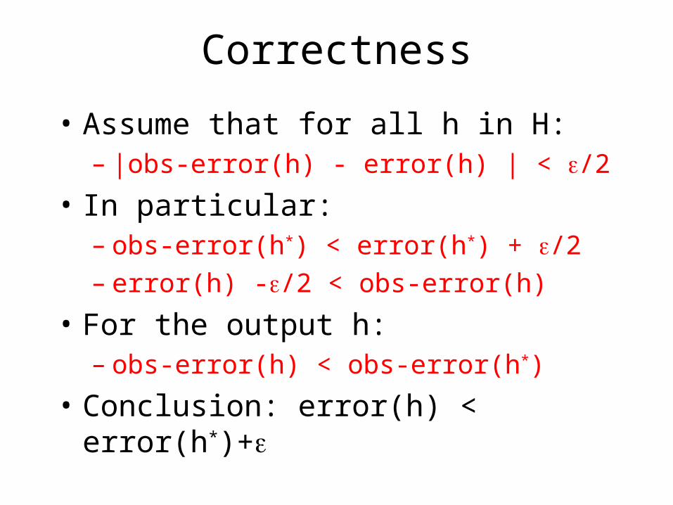
Correctness

• Assume that for all h in H:– |obs-error(h) - error(h) | < /2

• In particular:– obs-error(h*) < error(h*) + /2– error(h) -/2 < obs-error(h)

• For the output h:– obs-error(h) < obs-error(h*)

• Conclusion: error(h) < error(h*)+

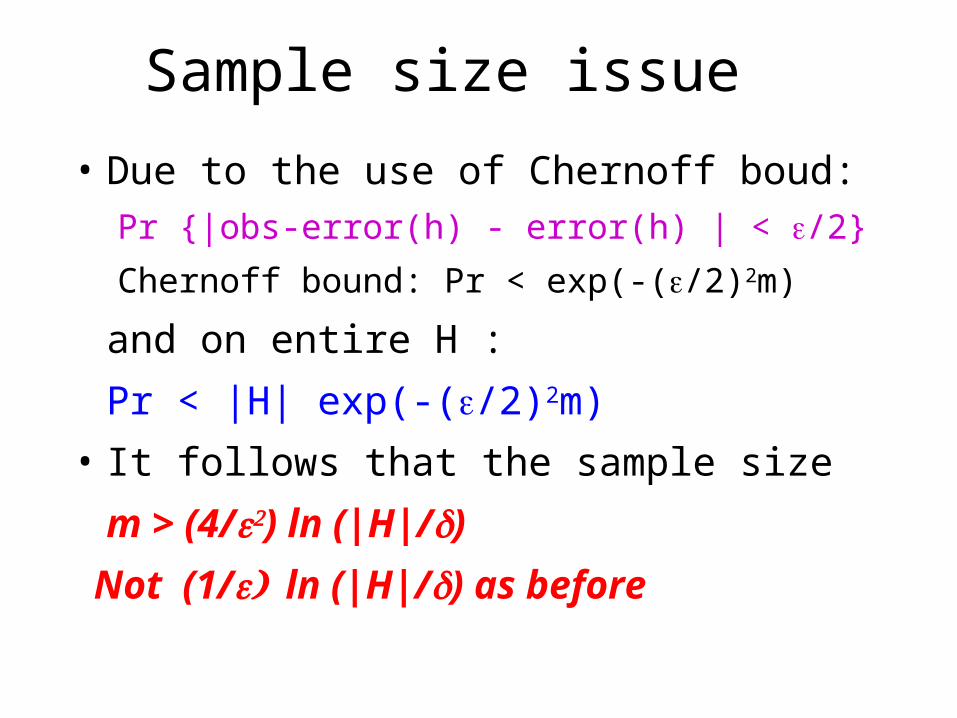
Sample size issue

• Due to the use of Chernoff boud:Pr {|obs-error(h) - error(h) | < /2}

Chernoff bound: Pr < exp(-(/2)2m)

and on entire H :

Pr < |H| exp(-(/2)2m)

• It follows that the sample size

m > (4/) ln (|H|/) Not (1/ln (|H|/) as before

Example: Learning OR of literals

• Inputs: x1, … , xn

• Literals : x1,

• OR functions:• For each variable, target

disjunction may contain xi or not, thusNumber of disjunctions is 3n

1x

741 xxx

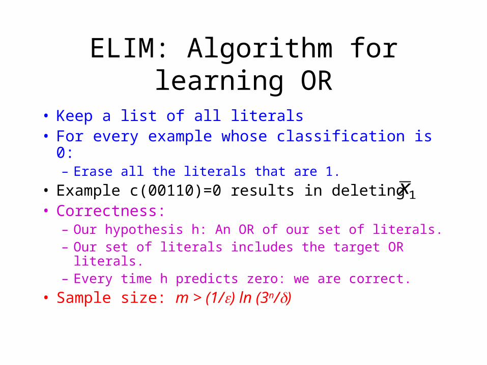
ELIM: Algorithm for learning OR

• Keep a list of all literals• For every example whose classification is 0:

– Erase all the literals that are 1.

• Example c(00110)=0 results in deleting • Correctness:

– Our hypothesis h: An OR of our set of literals.– Our set of literals includes the target OR literals.– Every time h predicts zero: we are correct.

• Sample size: m > (1/) ln (3n/)

1x

Learning parity

• Functions: x1 x7 x9

• Number of functions: 2n

• Algorithm:– Sample set of examples– Solve linear equations (Matrix exists)

• Sample size: m > (1/) ln (2n/)

Infinite Concept class

• X=[0,1] and H={c | in [0,1]}

• cxiff x <

• Assume C=H:

• Which c should we choose in [min,max]?

min

max

Proof I

• Define max = min{x|c(x)=1}, min = max{x|c(x)=0}

• _Show that the probability that – Pr[ D([min,max]) > ] <

• Proof: By Contradiction.– The probability that x in [min,max] at least – The probability we do not sample from

[min,max]Is (1-)m

– Needs m > (1/) ln (1/)

There is something wrong

Proof II (correct):

• Let max’ be : D([,max’])=/2• Let min’ be : D([,min’])=/2• Goal: Show that with high probability

– X+ in [max’,] and

– X- in [,min’]

• In such a case any value in [x-,x+] is good.

• Compute sample size!

Proof II (correct):

• Pr{x1,x2,..,xm} is not in [,min’])=

(1- /2)m < exp(-m/2)• Similarly with the other side• We require 2exp(-m/2) < δ• Thus, m > 2/ln(2/δ)

Comments

• The hypothesis space was very simple H={c | in [0,1]}

• There was no noise in the data or labels

• So learning was trivial in some sense (analytic solution)

Non-Feasible case: Label Noise

• Suppose we sample:

• Algorithm:– Find the function h with lowest error!

Analysis

• Define: zi as an 4 - net (w.r.t. D)

• For the optimal h* and our h there are– zj : |error(h[zj]) - error(h*)| < /4

– zk : |error(h[zk]) - error(h)| < /4

• Show that with high probability:– |obs-error(h[zi])-error(h[zi])| < /4

Exercise (Submission Mar 29, 04)

1. Assume there is Gaussian (0,σ) noise on xi. Apply the same analysis to compute the required sample size for PAC learning. Note: Class labels are determined by the non-noisy observations.

General -net approach

• Given a class H define a class G– For every h in H– There exist a g in G such that– D(g h) <

• Algorithm: Find the best h in H.• Computing the confidence and

sample size.

Occam Razor

W. Occam (1320) “Entities should

not be multiplied unnecessarily”

A. Einstein “Simplify a problem as

much as possible, but no simpler”

Information theoretic ground?

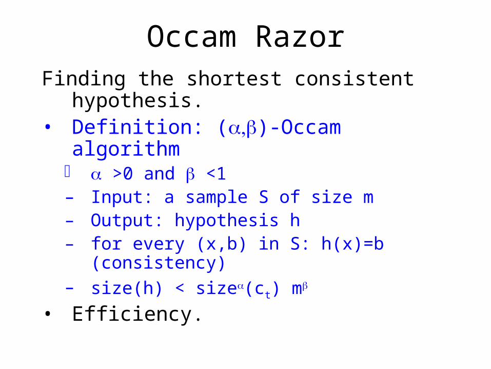
Occam RazorFinding the shortest consistent

hypothesis.• Definition: ()-Occam algorithm

>0 and <1– Input: a sample S of size m– Output: hypothesis h– for every (x,b) in S: h(x)=b

(consistency)– size(h) < size(ct) m

• Efficiency.

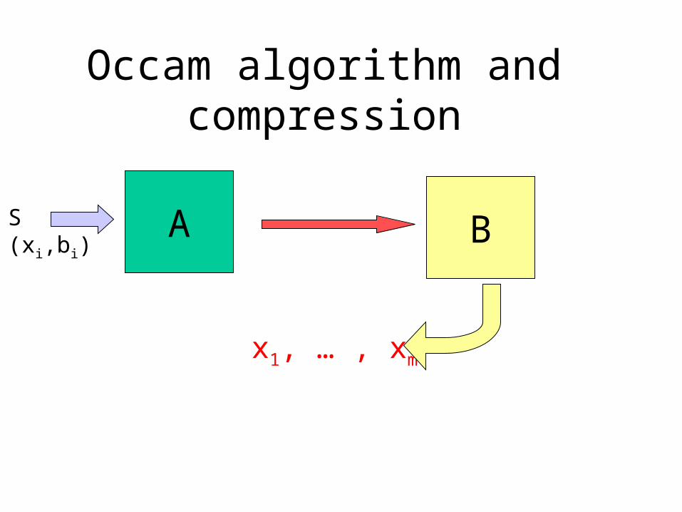
Occam algorithm and compression

A BS(xi,bi)

x1, … , xm

Compression

• Option 1:– A sends B the values b1 , … , bm

– m bits of information• Option 2:

– A sends B the hypothesis h– Occam: large enough m has size(h) < m

• Option 3 (MDL):– A sends B a hypothesis h and

“corrections”– complexity: size(h) + size(errors)

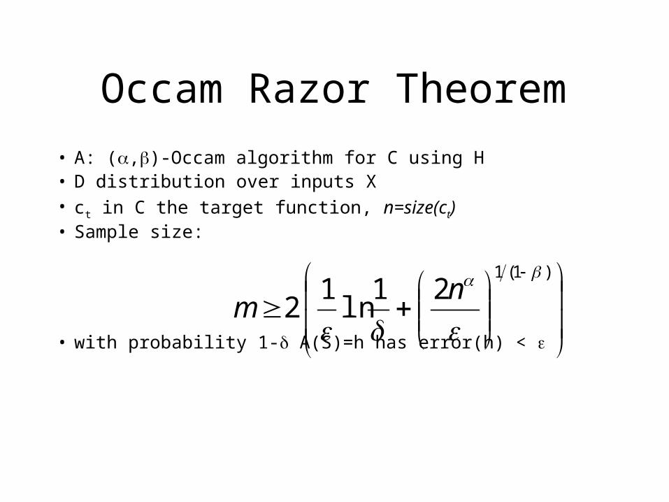
Occam Razor Theorem

• A: (,)-Occam algorithm for C using H• D distribution over inputs X• ct in C the target function, n=size(ct)• Sample size:

• with probability 1- A(S)=h has error(h) <

)1(121

ln1

2

n

m

Occam Razor Theorem• Use the bound for finite hypothesis class.• Effective hypothesis class size 2size(h)

• size(h) < n m

• Sample size:

1ln

12lnln

1 2 mn

mmn

The VC dimension will replace 2size(h)

Exercise (Submission Mar 29, 04)

2. For an (,)-Occam algorithm, givennoisy data with noise ~ (0, σ2) find the limitations on m.

Hint (ε-net and Chernoff bound)

Learning OR with few attributes

• Target function: OR of k literals• Goal: learn in time:

– polynomial in k and log n and constant

• ELIM makes “slow” progress – disqualifies one literal per round– May remain with O(n) literals

Set Cover - Definition

• Input: S1 , … , St and Si U

• Output: Si1, … , Sik and j Sjk=U

• Question: Are there k sets that cover U?

• NP-complete

Set Cover Greedy algorithm

• j=0 ; Uj=U; C=

• While Uj – Let Si be arg max |Si Uj|

– Add Si to C

– Let Uj+1 = Uj – Si

– j = j+1

Set Cover: Greedy Analysis

• At termination, C is a cover.• Assume there is a cover C’ of size k.

• C’ is a cover for every Uj

• Some S in C’ covers Uj/k elements of Uj

• Analysis of Uj: |Uj+1| |Uj| - |Uj|/k

• Solving the recursion.• Number of sets j < k ln |U| • Ex 2 Solve

• Lists of arbitrary size can represent any

boolean function. Lists with tests of at most

with at most k < n literals define the k-DL

boolean language. For n attributes, the

language is k-DL(n).

• The language of tests Conj(n,k) has at most

3|Conj(n,k)| distinct component sets (Y,N,absent)

• |k-DL(n)| 3|Conj(n,k)| |Conj(n,k)|! (any order)

• |Conj(n,k)| = i=0 ( ) = O(nk)

Learning decision lists

2n i

k

Building an Occam algorithm

• Given a sample S of size m– Run ELIM on S – Let LIT be the set of literals– There exists k literals in LIT that

classify correctly all S

• Negative examples: – any subset of LIT classifies theme

correctly

Building an Occam algorithm

• Positive examples: – Search for a small subset of LIT – Which classifies S+ correctly– For a literal z build Tz={x | z satisfies x}– There are k sets that cover S+

– Find k ln m sets that cover S+

• Output h = the OR of the k ln m literals • Size (h) < k ln m log 2n• Sample size m =O( k log n log (k log n))

Criticism of PAC model

• The worst-case emphasis makes it unusable– Useful for analysis of computational complexity– Methods to estimate the cardinality of the

space of concepts (VC dimension). Unfortunately not sufficiently practical

• The notions of target concepts and noise-free training are too restrictive– True. Switch to concept approximation weak.– Some extensions to label noise and fewer to

variable noise

Summary

• PAC model– Confidence and accuracy– Sample size

• Finite (and infinite) concept class• Occam Razor

References

• A theory of the learnable. Comm. ACM 27(11):1134-42, 1984. Original work

• Probably approximately correct learning. D. Haussler. (Review)

• Efficient noise-tolerant learning from statistical queries. M. Kearns. (Review on noise methods)

• PAC learning with simple examples. F. Denis et al. (Simple)

Learning algorithms

• OR function • Parity function• OR of a few literals• Open problems

– OR in the non-feasible case– Parity of a few literals