Probability theory: (lecture 2 on AMLbook.com)maximum likelihood estimation (MLE)

get parameters from dataHoeffding’s inequality (HI)

how good are my parameter estimates?Connection to learning

HI applies to relationship between Eout(h), Etest(h), and Ein(h)

Maximum Likelihood Parameter Estimation

• Estimate parameters q of a probability distribution given a sample X drawn from that distribution

• Example: estimate the mean and variance of a normal distribution

2Lecture Notes for E Alpaydın 2010 Introduction to Machine Learning 2e © The MIT Press (V1.0)

Form the likelihood function• Likelihood of q given the sample X

l(θ|X) = p (X |θ) = ∏t p(xt|θ)

• Log likelihood L(θ|X) = log(l(θ|X)) = ∑

t log p(xt|θ)

• Maximum likelihood estimator (MLE)θ* = argmaxθ L(θ|X)

the value of θ that maximizes L(θ|X)

3Lecture Notes for E Alpaydın 2010 Introduction to Machine Learning 2e © The MIT Press (V1.0)

Example: Bernoulli distribution

4Lecture Notes for E Alpaydın 2010 Introduction to Machine Learning 2e © The MIT Press (V1.0)

x = {0,1}x = 0 implies failure x = 1 implies success

po = probability of success:

parameter to be determined from data

p(x) = pox (1 – po )

(1 – x)

p(1) = po p(0)= 1 – po

p(1) + p(0)= 1 distribution is normalized

Given a sample of N trials,show that po = ∑

t xt / N = successes/trial

is the maximum likelihood estimate of p0

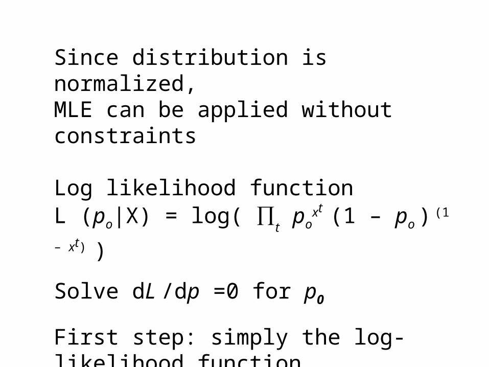
Since distribution is normalized,MLE can be applied without constraints

Log likelihood functionL (po|X) = log( ∏

t po

xt (1 – po ) (1 – xt) )

Solve dL /dp =0 for p0

First step: simply the log-likelihood function

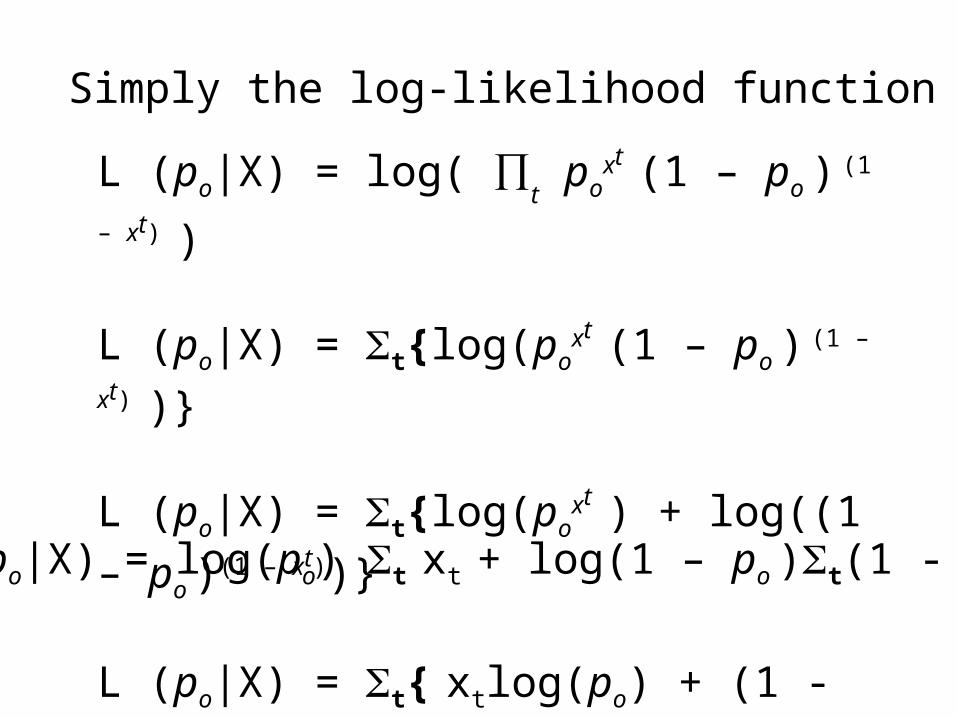
L (po|X) = log( ∏t po

xt (1 – po ) (1 – xt) )

L (po|X) = St{log(poxt (1 – po )

(1 – xt) )}

L (po|X) = St{log(poxt ) + log((1 – po )(1 – xt))}

L (po|X) = St{ xtlog(po) + (1 - xt )log(1 – po )}

Simply the log-likelihood function

L (po|X) = log(po) St xt + log(1 – po )St(1 - xt )

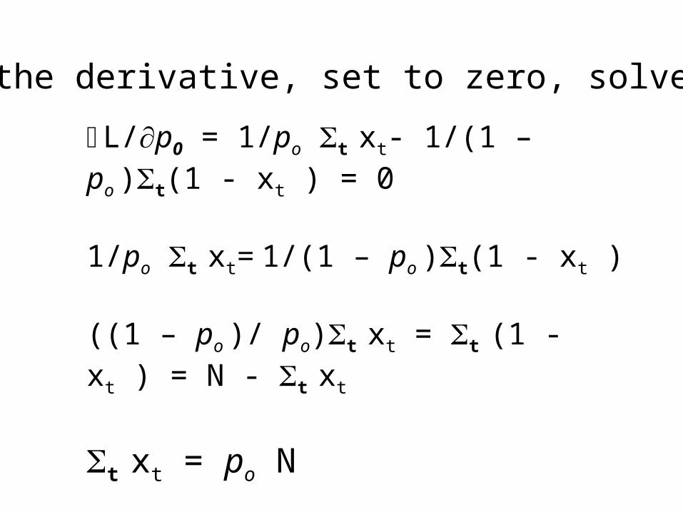
L/p0 = 1/po St xt- 1/(1 – po )St(1 - xt ) = 0

1/po St xt= 1/(1 – po )St(1 - xt )

((1 – po )/ po)St xt = St (1 - xt ) = N - St xt

St xt = po N

St xt / N = po

Take the derivative, set to zero, solve for p0

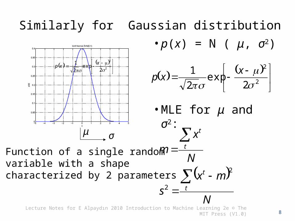
Similarly for Gaussian distribution

N

mxs

N

xm

t

t

t

t

2

2

• p(x) = N ( μ, σ2)

• MLE for μ and σ2:

8

2

2

2exp

2

1 x-xp

μ σ

2

2

22

1

x

xp exp

Lecture Notes for E Alpaydın 2010 Introduction to Machine Learning 2e © The MIT Press (V1.0)

Function of a single random variable with a shape characterized by 2 parameters

Pictorial representation of estimating a population mean by a sample mean

Confidence in estimate population mean depends onsample size

Let d = 2exp(-2e2N) Solve for e(d,N) = sqrt(ln(2/d)/2N)

H.I. says that we know |m-n|< e(d,N) with probability at least 1-d

Hoeffding’s inequality

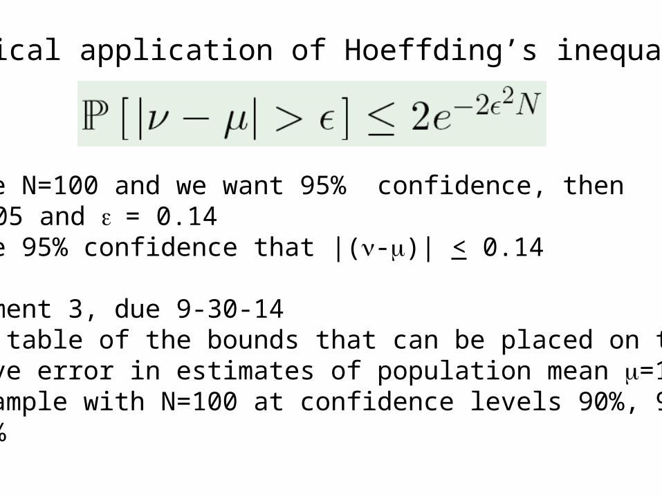
Suppose N=100 and we want 95% confidence, thend = 0.05 and e = 0.14We have 95% confidence that |(n-m)| < 0.14

Assignment 3, due 9-30-14Make a table of the bounds that can be placed on the relative error in estimates of population mean m=1 based on a sample with N=100 at confidence levels 90%, 95%, and 99%

Typical application of Hoeffding’s inequality

For a specific hypothesis h, Eout(h) is analogous to the population mean. Ein(h) is analogous to a sample mean

For a specific hypothesis h, Hoeffding’s inequality applies if the sample on which Ein(h) is evaluated was not used in the selection of h.

Usually, h is optimum member of an hypothesis set chosen by application of training data and Ein(h) is evaluated on a test set.

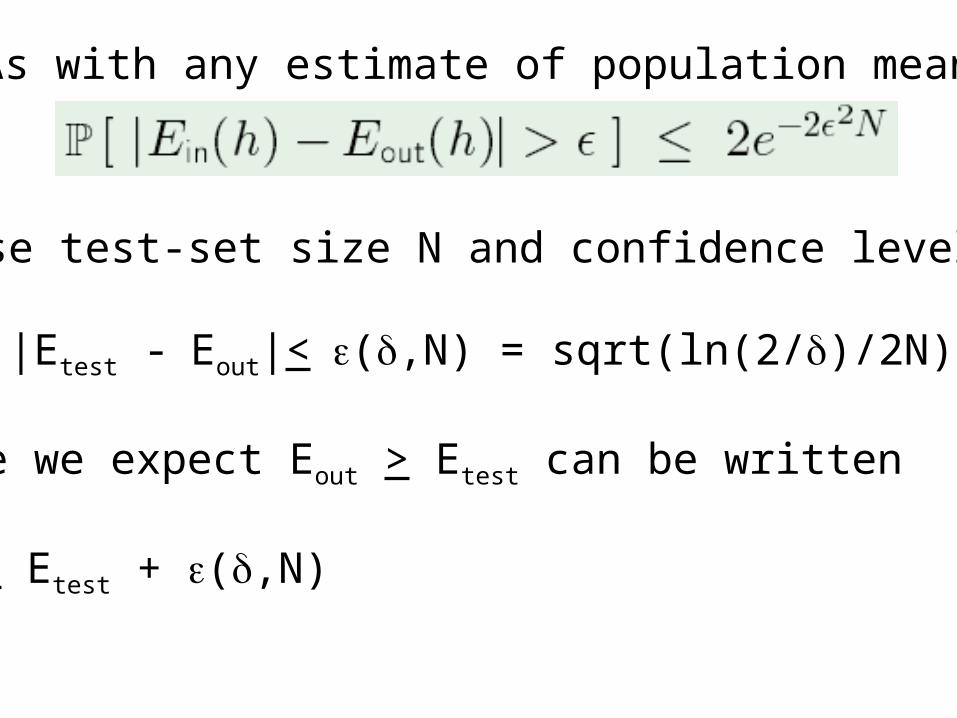
Choose test-set size N and confidence level 1-d then |Etest - Eout|< e(d,N) = sqrt(ln(2/d)/2N)

Since we expect Eout > Etest can be written

Eout < Etest + e(d,N)

As with any estimate of population mean

Test set dilemma

To obtain meaningful confidence from Hoeffding’s inequality may require Ntest so large that training is compromised.

In chapter 4 of text authors discuss a method to calculate Etest(h) that does not greatly diminish the data available for training.

Review: Probability theory(see lecture 2 on AMLbook.com)maximum likelihood estimation (MLE)

get parameters from dataHoeffding’s inequality (HI)

how good are my parameter estimates?Connection to learning

HI applies to relationship between Eout(h) and Etest(h)

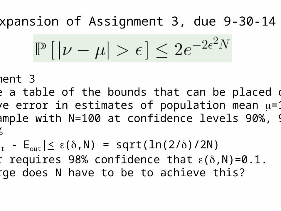
Assignment 31) Make a table of the bounds that can be placed on the relative error in estimates of population mean m=1 based on a sample with N=100 at confidence levels 90%, 95%, and 99%2) |Etest - Eout|< e(d,N) = sqrt(ln(2/d)/2N)Sponsor requires 98% confidence that e(d,N)=0.1. How large does N have to be to achieve this?

Expansion of Assignment 3, due 9-30-14

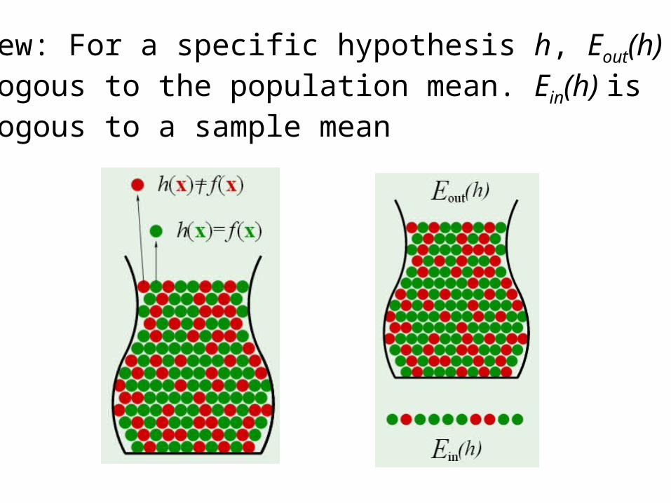
Review: For a specific hypothesis h, Eout(h) is analogous to the population mean. Ein(h) is analogous to a sample mean

HI applies to relationship between Eout(h) and Ein(h)

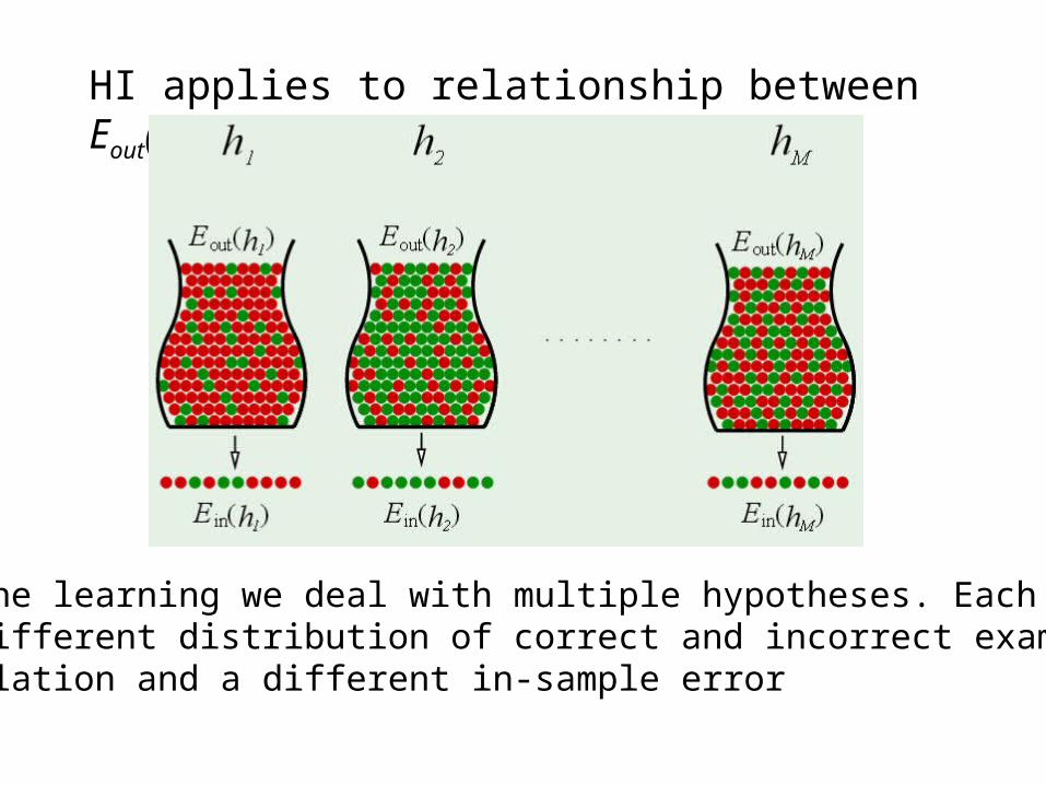
In machine learning we deal with multiple hypotheses. Each h can have a different distribution of correct and incorrect examples in the population and a different in-sample error

Each test of an hypothesis is an independent event

One of these events has the smallest Ein(h) and determines the optimum hypothesis g

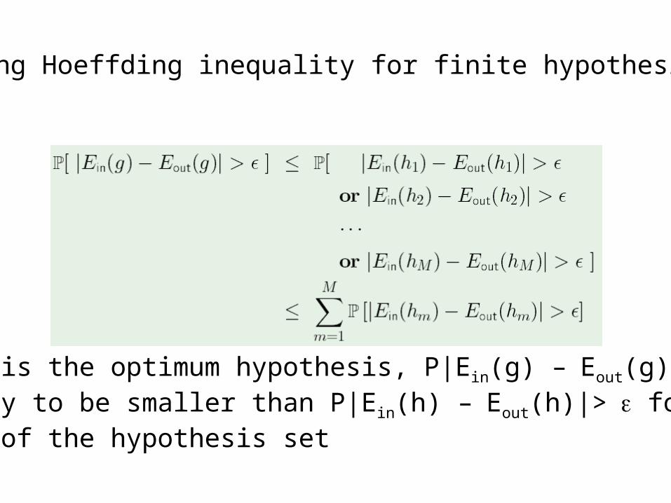
Modifying Hoeffding inequality for finite hypothesis set

Since g is the optimum hypothesis, P|Ein(g) – Eout(g)|> e is likely to be smaller than P|Ein(h) – Eout(h)|> e for most members of the hypothesis set

“union bound” approximation

If P|Ein(g) – Eout(g)|> e is smaller than P|Ein(h) – Eout(h)|> e for most members of the hypothesis set, it is certainly smaller than their sum.

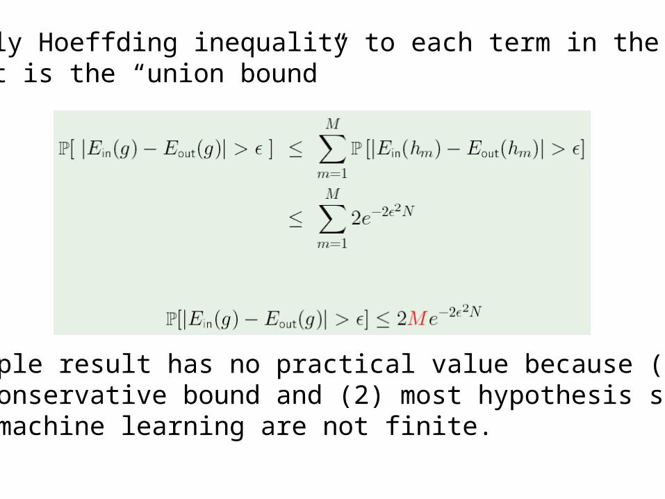
Apply Hoeffding inequality to each term in the sum that is the “union bound”

This simple result has no practical value because (1) it is a very conservative bound and (2) most hypothesis sets used in machine learning are not finite.

Feasibility of learning

Union bound approximation shows “feasibility of learning” for finite hypothesis sets.For any (e,d), P[|Ein(g) – Eout(g)|> e] <d by sufficiently large N

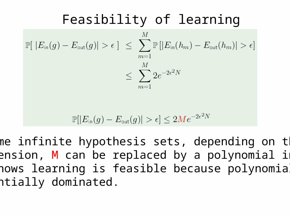
Feasibility of learning

For some infinite hypothesis sets, depending on their VG dimension, M can be replaced by a polynomial in N. This shows learning is feasible because polynomials are exponentially dominated.