probability in philosophy - brian weatherson - home pagebrian.weatherson.org/pl2.pdf · ·...

Probability in Philosophy

Brian Weatherson

Rutgers and Arche

June, 2008

Brian Weatherson (Rutgers and Arche) Probability in Philosophy June, 2008 1 / 90

Revision and CleanUp

Probability Functions

A probability function with respect to an entailment relation ` has asdomain a set S of propositions closed under conjunction, disjunction andnegation, and as range R), and satisfies the following four axioms for allA, B ∈ S

1 If A is a `-theorem, then Pr(A) = 1

2 If A is a `-antitheorem, then Pr(A) = 0

3 If A ` B, then Pr(A) ≤ Pr(B)

4 Pr(A) + Pr(B) = Pr(A ∨ B) + Pr(A ∧ B)



Classical Probability

If ` is classical implication, those axioms can be simplified a lot.

We can replace the third axiom with an axiom stating tautologieshave probability 1

And we can replace the fourth axiom with an axiom saying Pr(A) +Pr(B) = Pr(A ∨ B) when A and B are disjoint



Classical Probability

I showed last time that we could prove (classically) that if allequivalent propositions had the same probability, then if A entailed B,B’s probability was not less than A

I should have noted we could start with something (apparently)weaker

We can prove that if all tautologies have probability 1, thenequivalent propositions have the same probability

Assume A and B are equivalent

Then A ∨¬B is a tautology, and A and ¬B are disjoint

So Pr(A) + Pr(¬B) = 1, so Pr(A) = 1 - Pr(¬B). But Pr(B) = 1 -Pr(¬B), so Pr(A) = Pr(B)



Truth Tables

In circumstances where classical truth tables are useful modellingdevices, there’s a simple way to think about probability.

So imagine you’re in a setting where (a) you don’t care about theinternal structure of atomic propostions, and (b) you’ve only gotfinitely many atomic propositions to consider.

In such circumstances, probability theory is basically measure theoryover the rows of the truth table.

That is, you generate probability functions by assigning a number (ameasure) to each row of the truth tables such that each measure isnon-negative, and the measures sum to 1.

Then Pr(A) is the sum of the measures of the rows on which A is true.



Conditional Probability Introduced

As well as being interested in the probability of events (e.g. whetherit will rain tomorrow), we’re sometimes interested in probabilitiesconditional on other events (e.g. whether it will rain tomorrowconditional on rain being forecast).

There is a standard definition for the conditional probability of Bgiven A.

Pr(A|B) =dfPr(AB)

Pr(B), if Pr(B) > 0



Independence

We say that A and B are probabilistically independent iff Pr(AB) =Pr(A)Pr(B).This is equivalent to each of the following claims, which in turn justify thename.

Pr(A|B) = Pr(A)

Pr(B|A) = Pr(B)

The intuitive idea is that taking one as given doesn’t change the other.



Recovering Unconditional Probability

We now take ”Pr(A)” to be a shorthand for Pr(A|T), where T is sometautology

Again, if the logic is classical, the previous axioms can be simplifiedsomewhat

The idea still is that conditional on any C, probabilities are in [0, 1],logical truths/falsehoods take the extreme values, logically weakerpropositions have a higher probability, and the probability of adisjunction of exclusive disjuncts is the sum of the probability of thedisjuncts.

When we don’t care about the background C, we can use the simpleaxiom Pr(AB) = Pr(A|B)Pr(B)



An Important Theorem

Pr(A) = Pr(AB) + Pr(A¬B)

Pr(AB) = Pr(A|B)Pr(B)

Pr(A¬B) = Pr(A|¬B)Pr(¬B)

Pr(A) = Pr(A|B)Pr(B) + Pr(A|¬B)Pr(¬B)

Note it follows from this that Pr(A|B) and Pr(A|¬ B) can’t be on the’same side’ of Pr(A), either both greater than Pr(A) or both less thanPr(A). We’ll prove this in two sections time.



Cleaning Up

I mentioned last time that some of the foundational proofs relied onclassical logic, but I didn’t prove this.

I don’t have a particularly good answer as to how much workdistributivity principles on the underlying lattice do.

But I can say a bit about how much the fact that the underlying logicis classical does.

In intuitionistic probability, it’s impossible to get from the equality ofthe probability of equivalent propositions, to the claim that weakerpropositions have greater probability.

And it is impossible to get from the ’simple’ addition axiom Pr(A) +Pr(B) = Pr(A ∨ B) for disjoint A, B to the ’general’ axiom Pr(A) +Pr(B) = Pr(A ∨ B) + Pr(A ∧ B).



Weaker Propositions are More Probable?

This might be too much ’inside baseball’ for those of you who don’tcare about intuitionistic logic, but it won’t take too long.

Consider a Kripke model with W = {1, 2, 3, 4}, R ={< 1, 1 >, < 1, 2 >, < 1, 3 >, < 1, 4 >, < 2, 2 >, < 2, 3 >,< 3, 3 >, < 4, 4 >} and V(p) = {3}.Define a ’measure’ m such thatm(1) = 0.3, m(2) = −0.1, m(3) = 0.5, m(4) = 0.3.

Then define Pr(A) = the sum of m(x) over the x that force A

That satisfies the addition axiom, and equivalent propositions getequal probability, but Pr(p) = 0.5, while Pr(¬¬p) = 0.4



Simple and General Addition

This one is a bit easier

Consider a language with just two atomic variables, p and q

Define a Pr such that Pr(A) = 1 if A is an intuitionistic consequenceof p ∨ q, and 0 otherwise

That satisfies all the axioms we’ve considered except the generaladdition axiom, which fails because Pr(p) = Pr(q) = Pr(p ∧ q) = 0,while Pr(p vee q) = 1.


Countable Additivity

Infinitary Addition

Sometimes infinite sums don’t seem to be well defined

For instance, no real number is the intuitive sum of 1+2+3+...

For a different reason, no real number is the intuitive sum of1-1+1-1+1...

We could say that’s (1-1)+(1-1)+... = 0+0+... = 0

Or we could say that it is 1+(-1+1)+(-1+1)+... = 1+0+0+... = 1

Better to say it is not defined at all



Limits of Sums

But some sums converge on a stable value.

That is, as we keep on adding terms we get closer and closer to aparticular value.

In that case, we say the sum is the value we converge on.

More formally, if x1, x2, ... are such that

∃s.∀e > 0.∃k ∈ N.∀n > k .

n∑j=1

xj ∈ (s − e, s + e)

We’ll say that s = x1 + x2 + ....



Sums of Probabilities

One can prove (assuming classical mathematics), that if x1, x2, ... arethe probabilities of disjoint propositions p1, p2, ..., then x1 + x2 + ...exists.

This is a consequence of a more general result that if ∀i .xi ≥ 0 and∃s∀n

∑nk=1 xk < s, then x1 + x2 + ... exists.

So it might make sense to ask whetherPr(p1 ∨ p2 ∨ ...) = Pr(p1) + Pr(p2) + ...



Some Interesting Limiting Sums

It’s useful to remember a few examples of limits in order to work withvarious examples.

The most crucial result for our purposes is∞∑

k=1

r−k =1

r − 1

So, for instance, 13 + 1

9 + ... = 12



An Open Question

Say that for each n ∈ 1, 2, ..., the probability that that there are exactly njabberwocks is 1

2n+1 .

What is the probability that there is at least 1 jabberwock?



An Open Question

You might try to reason as follows

The probability that there is at least 1 jabberwock is the probabilitythat there’s exactly 1, plus the probability that there’s exactly 2 plusetc

That is, it’s 14 + 1

8 + ...

That is, it’s 12

That reasoning is not sound given the axioms to date.



Inequality or Equality

The ’addition’ axiom we have only works for pairwise addition. You can’tinfer much from that about infinitary addition.

You can infer something

Finite addition tells us the probability that there are between 1 and njabberwocks, for any n

And as n goes to infinity, that probability goes to 0.5

Since that proposition entails there are some jabberwocks, theprobability that there are some jabberwocks is at least 0.5



Inequality or Equality

In general, if p1, p2, ... are pairwise inconsistent, the most we can prove is

Pr(p1 ∨ p2 ∨ ...) ≥ Pr(p1) + Pr(p2) + ...

If we want equality, we have to add it as an axiom.



The Flat Distribution Over N

There is a reason some people resist adding this as an axiom.

It would rule out a flat distribution over N

Let the domain be subsets of NLet Fn be the number of numbers ≤n such that F(n), for anypredicate F, and define Pr as follows

Pr(Fa|Ga) = limn→∞

Fn

(F ∧ G )n

That would be ruled out by the equality axiom.




There is a reason some people resist adding this as an axiom.

It would rule out a flat distribution over NLet the domain be subsets of NLet Fn be the number of numbers ≤n such that F(n), for anypredicate F, and define Pr as follows

Pr(Fa|Ga) = limn→∞

Fn

(F ∧ G )n

That would be ruled out by the equality axiom.




The flat distribution says that Pr(a = n) = 0 for all n

But it says that Pr(a = 1 ∨ a = 2 ∨ ... ) = 1

Indeed, any distribution that says that there are a countable infinity ofchoices, and each is equally probable, will have this feature

Some people (including me!) take that as a proof that there can’t bea probability distribution making each member of a countable infinityequally probable

Other people take it as a proof thatPr(p1 ∨ p2 ∨ ...) = Pr(p1) + Pr(p2) + ... if (p1, p2, ... are pairwisedisjoint) is not an axiom



New Axiom

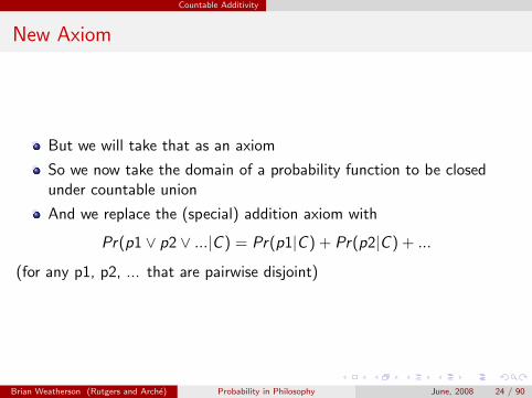
But we will take that as an axiom

So we now take the domain of a probability function to be closedunder countable union

And we replace the (special) addition axiom with

Pr(p1 ∨ p2 ∨ ...|C ) = Pr(p1|C ) + Pr(p2|C ) + ...

(for any p1, p2, ... that are pairwise disjoint)



Terminology

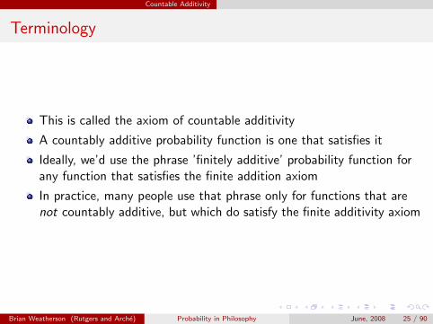
This is called the axiom of countable additivity

A countably additive probability function is one that satisfies it

Ideally, we’d use the phrase ’finitely additive’ probability function forany function that satisfies the finite addition axiom

In practice, many people use that phrase only for functions that arenot countably additive, but which do satisfy the finite additivity axiom


A Little Set Theory

Same Size Sets

I should say a little more about what I mean by a ’countable’ set, andhere is as good a time as any to do it

There is an interesting question about what it is to say sets are thesame size

The working definition that most mathematicians use is Cantor’s

Two sets are the same size iff there is a one-one mapping from one tothe other


A Little Set Theory

Cantor’s Definition

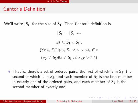
We’ll write |S1| for the size of S1. Then Cantor’s definition is

|S1| = |S2| ↔

∃f ⊆ S1 × S2 :

(∀x ∈ S1∃!y ∈ S2 :< x , y >∈ f )∧

(∀y ∈ S2∃!x ∈ S1 :< x , y >∈ f )

That is, there’s a set of ordered pairs, the first of which is in S1, thesecond of which is in S2, and each member of S1 is the first memberin exactly one of the ordered pairs, and each member of S2 is thesecond member of exactly one.


A Little Set Theory

Nice Consequences

This gives us just the results we want for finite cases

Any two sets with n members are the same size, for any finite n

And it does so without assuming there are such things as naturalnumbers

So in principle it could be used to measure the size of infinite sets


A Little Set Theory

Odd Consequences

When we do so, we get some odd results

Let S1 be the set of natural numbers, and S2 the set of even numbers

Then there’s an easy mapping from one to the other, the mapping< 1, 2 >, < 2, 4 >, ....

So it turns out these sets are the same size

So a set can be the same size as one of its proper subsets


A Little Set Theory

Cantor’s Definition

For reasons too numerous to go into here, mathematical orthodoxy isthat we should accept this odd result

And philosophers have (I think correctly) followed them

There is a useful generalisation of Cantor’s generalisation that wewon’t prove, but is useful to have

If there is a mapping from S1 to a subset of S2, and from S2 to asubset of S1, then there is a mapping from S1 itself to S2.

We’ll often use that to prove sets are the same size


A Little Set Theory

Powersets

When you first see the odd result, you might be tempted to concludethat all infinite sets are the same size

That’s not a consequence of Cantor’s definition

In fact we can prove a rather important result inconsistent with it

The powerset of S is the set of all subsets of S (including the null setand S itself)

We’ll write this P(S)

We can prove |P(S)| 6= |S|


A Little Set Theory

Powersets

Assume |P(S)| = |S|Then there is a mapping f from S to P(S)

Let R = x : x ∈ S ∧ x /∈ f (x)

Since by definition R ⊆ S, R ∈ P(S)

So there must be some y ∈ S that is mapped onto R, i.e. f(y) = R

If y ∈ R, then y /∈ f(y), so y /∈ R

But if y /∈ R, then y ∈ S and y /∈ f(y), so y ∈ R

Contradiction


A Little Set Theory

Countable and Uncountable Sets

As always, let N be the set of natural numbers.

One consequence of the above result is that some sets, for exampleP(N) are not the same size as N.

We’ll say that sets that are the same size as N are countable.

We won’t prove it here, but it is provable that R is the same size asP(N), a fact we’ll use a bit in what follows


A Little Set Theory

Set of all Sets

One consequence of |P(S)| > |S| is that there is no set of all sets

To see this, assume S is the set of all sets

Then P(S) ⊆ S, since every member of P(S) is a set

So |P(S)| ≯ |S|, contrary to what we proved above


A Little Set Theory

Consequences for Probability

Recall that when we were setting things up formally, probabilitieswere defined over sets of sets, the latter of which we sometimes tookto be propositions

The set that the probability is defined over can’t be the set of all sets,because there is no such set

As we’ll go along, we’ll see more and more reasons for thinking thatthere are serious limits to which propositions can have probabilities

This matters philosophically I think; there are a lot of applicationswhere people assume that every proposition has a probability, and thisassumption is typically false.


Conglomerability

Finite Conglomerability

We say that a probability function is finitely conglomerable iff there isno proposition H and partition E1, E2, ..., En such that either for all i,Pr(H|Ei ) > Pr(H), or for all i, Pr(H|Ei ) < Pr(H).

By ’partition’ here we mean a set of propositions that are mutuallyexclusive and jointly exhaustive

Given the axioms (and classical logic, which we’re assuming basicallyalways from now on) we can prove that all probability functions arefinitely conglomerable.


Conglomerability

Proof of Finite Conglomerability

Assume that ∀i .Pr(H|Ei ) > Pr(H). (The other case works the same way.)

Pr(H) = Pr(HE1 ∨ HE2 ∨ ... ∨ HEn)

= Pr(HE1) + Pr(HE2) + ... + Pr(HEn)

= Pr(H|E1)Pr(E1) + Pr(H|E2)Pr(E2) + ... + Pr(H|En)Pr(En)

> Pr(H)Pr(E1) + Pr(H)Pr(E2) + ... + Pr(H)Pr(En)

= Pr(H)(Pr(E1) + Pr(E2) + ... + Pr(En))

= Pr(H)Pr(E1 ∨ E2 ∨ ... ∨ En)

= Pr(H)


Conglomerability

Finite Congolomerability

Conglomerability has a nice translation into regular talk

It says that the probability of H can’t be outside the realm of theprobability of H given possible evidence Ei

So it is a nice result to have, because that seems like it should be thecase


Conglomerability

Exclusive and Inclusive Disjunction

You might be reminded by conglomerability of principles likeor-elimination in logic

If we have Ei →H for each i in a partition E1, E2, ..., En , then wehave H

Similarly, if Pr(H|Ei ) > x for each i, then Pr(H) > x

But these principles are not the same

The logical rule holds for either inclusive or exclusive disjunction

The probabilistic rule only holds for exclusive disjunction


Conglomerability

Not a Counterexample

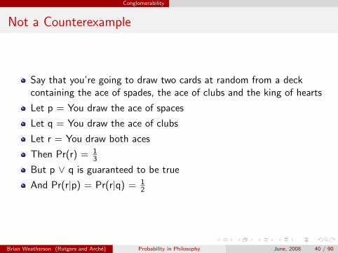
Say that you’re going to draw two cards at random from a deckcontaining the ace of spades, the ace of clubs and the king of hearts

Let p = You draw the ace of spaces

Let q = You draw the ace of clubs

Let r = You draw both aces

Then Pr(r) = 13

But p ∨ q is guaranteed to be true

And Pr(r|p) = Pr(r|q) = 12


Countable Conglomerability


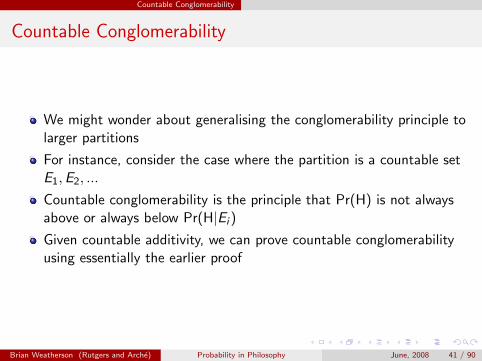
We might wonder about generalising the conglomerability principle tolarger partitions

For instance, consider the case where the partition is a countable setE1, E2, ...

Countable conglomerability is the principle that Pr(H) is not alwaysabove or always below Pr(H|Ei )

Given countable additivity, we can prove countable conglomerabilityusing essentially the earlier proof



Proof of Countable Congolomerability

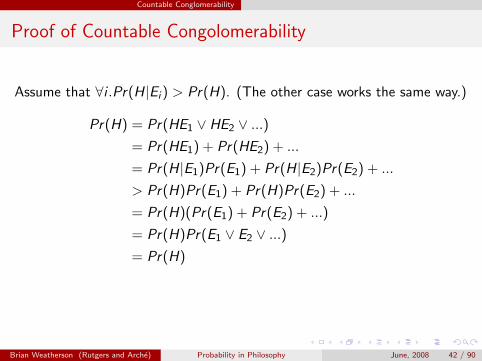
Assume that ∀i .Pr(H|Ei ) > Pr(H). (The other case works the same way.)

Pr(H) = Pr(HE1 ∨ HE2 ∨ ...)

= Pr(HE1) + Pr(HE2) + ...

= Pr(H|E1)Pr(E1) + Pr(H|E2)Pr(E2) + ...

> Pr(H)Pr(E1) + Pr(H)Pr(E2) + ...

= Pr(H)(Pr(E1) + Pr(E2) + ...)

= Pr(H)Pr(E1 ∨ E2 ∨ ...)

= Pr(H)



The Flat Distribution Again

That proof used countable additivity twice over

We might wonder whether it is necessary

The answer is that it is

Indeed the flat distribution we’ve seen provides a nice counterexampleto countable conglomerability



Violating Conglomerability

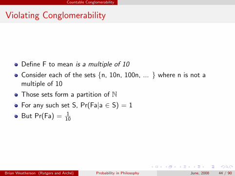
Define F to mean is a multiple of 10

Consider each of the sets {n, 10n, 100n, ... } where n is not amultiple of 10

Those sets form a partition of NFor any such set S, Pr(Fa|a ∈ S) = 1

But Pr(Fa) = 110



A More Dramatic Violation

Assume i and j are numbers randomly chosen from NConsider Pr(i > j)

It’s easy enough to show that ∀n. Pr(i > j | i = n) = 0

And ∀n. Pr(i > j | j = n) = 1

Whatever value Pr(i > j) takes, we’ll have a massive conglomerabilityfailure



Generalising This Result

So we’ve shown that if we assume countable additivity, we can provecountable conglomerability

And without countable additivity, this proof doesn’t go through

I was hoping to find a proof of something stronger

Namely that if Pr is not countably additive and its domain is closedunder countable union, then Pr is not countably conglomerable

But I couldn’t find a proof of that, or a citation of it, or acounterexample

I’ll keep looking and hopefully find something for next week


Conglomerability in Decision Theory


A decision-based version of finite conglomerability is central toorthodox decision theory

First some terminology

Let A � B mean that A is preferred to B

Let A � B mean that A is at least as preferred as B

Intuitively, conditional preferences are just preferences overconjunctions. So if A is preferred to B given C, that just means AC �BC




Assume throughout that E1, ..., En is a partition of possibility space.

Conglomerability for Preference (∀i .EiA � EiB)→ A � B

That is, if A is better than B conditional on any member of the partition,A is better than B

Again, note the importance of this being a partition

This really isn’t just or-elimination

On the other hand, it’s a pretty plausible principle



Utility Functions

To see how this generalises to the infinite case, we need a littledecision theory

Decision theorists attribute to each agent a utility function u. (We’reskipping for now the reasons they do this.)

If A � B, then u(A) > u(B)

More importantly, u measures strength of preference

Roughly, if A is preferred over B by as much as B is preferred over C,then u(A) - u(B) = u(B) - u(C)



Expected Value

Here is a general definition of the expected value of a random variable X.We’ll restrict our attention to the case where X takes on at most finitelymany values, because that’s all that’s needed for now.

Exp(X ) =∑k

k · Pr(X = k)

A random variable is just any expression that takes on different possiblevalues. So we can talk about the expected height of the next person thatwalks into the room, or the expected age of the next U.S. President, orthe expected utility of performing a particular action.

Note that this will frequently not be a possible value of X



Expected Value and Action

The core of modern decision theory is the idea that action A is preferredto action B iff the expected utility of doing A is higher than the expectedutility of doing B.

Here’s a quick example of this

If p is true, then u(A) = 10, and u(B) = 20

If p is false, then u(A) = 5 and u(B) = 1

And Pr(p) = 0.3

So Exp(u(A)) = 10 · 0.3 + 5 · 0.7 = 6.5

And Exp(u(B)) = 20 · 0.3 + 1 · 0.7 = 6.7

So B is better to do, although probably A will have the betteroutcome



The Two-Envelope Paradox

If we assume that u is unbounded above, i.e. that utilities can bearbitrarily high, we get a rather odd paradox

Formally, we can state the puzzle using two random variables, X andY

For each n ∈ 0, 1, 2, ..., Pr(X = 2n) = 25 ×

3n

5n

I’ll leave it as an exercise to prove that those probabilities sum to 1

Pr(Y=1) = Pr(Y=2) = 12

u(A) = XY, and u(B) = X(3-Y)




We can give a more intuitive characterisation of what’s going on

Take a biased coin, with a 35 chance of landing heads, two unmarked

envelopes, and put something worth 1 ’util’ in the first envelope

Flip the coin, and if it lands tails, skip to the next step, while if itlands heads, double the value (in utils) in the first envelope and repeat

Once the coin lands tails once, put double the amount in the secondenvelope

Now shuffle the envelopes, and offer one of them to a friend




Intuitively, it should not matter which envelope the friend receives

Let A be the action of taking the left-most envelope, and B takingthe right-most envelope

A little observation shows that the informal story we’ve told is wellmodelled by the formal story two slides back

Now we’ll try to argue that B is preferable to A.




We’ll write things like A=4 meaning that envelope A containssomething worth 4 utils

Conditional on A=1, we know B=2, so B is preferable to A

If A=2n, for n > 0, then there are two ways this could come about

Either X = 2n and Y = 1, so B = X = 2n+1, or X = 2n−1 and Y = 2,so B = 2n−1

The prior probability of the first of these is 3n

5n+1

And the prior probability of the second is 3n−1

5n




The prior probability of A = 2n and B = 2n+1 is 3n

5n+1

And the prior probability of A = 2n and B = 2n−1 is 3n−1

5n

Those are the only ways that A = 2n could come about

So Pr(A = 2n) = 3n

5n+1 + 3n−1

5n = 8×3n−1

5n+1

So Pr(B = 2n+1|A = 2n) =3n

5n+1

8×3n−1

5n+1

= 38

And from that it quickly follows that Pr(B = 2n−1|A = 2n) = 58




So conditional on envelope A containing 2n, there is a 38 chance that

B contains twice as much, and 58 chance that it contains 1/2 as much.

So conditional on envelope A containing 2n, the expected value of thecontents of B is38 × 2× 2n + 5

8 ×12 × 2n

And a little calculation shows that is equal to 1716 × 2n




In preference terms that we put before, we have the following true forall values of n

(Take envelope B)∧A = 2n �(Take envelope A)∧A = 2n

The conglomerability principle we were considering would say thatentails that (Take envelope B) � (Take envelope A)

Not so fast!

The exact same calculations show that for all n

(Take envelope A) ∧B = 2n �(Take envelope B)∧B = 2n

And conglomerability now says that (Take envelope A) � (Takeenvelope B)




We can put this all more dramatically

You know before looking that if you look in one of the envelopes,either of them, you’ll prefer to have the other

Indeed you’ll pay to have the other

And that’s true whichever envelope you look in

Some people take this to show that the setup is a money pump

We’ll say more about money pump arguments in subsequent lectures



A Puzzle About Conglomerability for Decisions

It seems we have to give up one of the following principles

1 � is anti-symmetric

2 u is unbounded above

3 Countable conglomerability for decisions

And if we give up 3, we have to give up one of

1 Countable conglomerablity for credences

2 That credences are governed by the same principles as decisions



Bad Company Objection?

If we take option 3, we have two somewhat distinct reasons for giving upcountable conglomerability for credences (i.e. subjective probabilities)

1 As we’ll see in upcoming weeks, some theorists think that allconstraints on credences follow from constraints on rational decisions.If that’s right, and we have to give up countable conglomerability fordecisions, there is a direct argument against countableconglomerability for credences

2 We might think that the intuitive support for countableconglomerability for credences is undermined by the inconsistency(relative to some assumptions) of countable conglomerability fordecisions. Think of this as a ’bad company’ argument.

We have to do a lot more work before we can evaluate these arguments.Some of that work has to do with ’flat’ distributions.


Flat Distributions

Logical Probability

Traditionally people thought of probability as a kind of ’logical’ relation

Consider again the model I mentioned of probabilities as measures ontruth tables

Given the way I set things up, there is one very natural measure youmight be pushed to

That’s the measure that assigns equal weight to each row

Something like this idea is behind the traditional ’logical’interpretation of probability


Flat Distributions

Logical Probability

This might seem like a bad idea, because probabilities will now bemassively model dependent

It would be nice to have something more precise to say at this pointabout what was driving the old idea

And by ’old’ here, I mean a view that was looking creaky whenKeynes wrote in the 1900s

To the extent that the view has modern adherents, they tend to havecomplicated views about what is the right model


Flat Distributions

Flat Distributions

There is a modern descendent of this old view though

That’s the view that when you are completely without evidence, youshould distribute credences/probabilities equally over open possibilities

If there are countably many open possibilities, that leads to violationsof countable additivity

In other cases it leads to worse results


Flat Distributions

United Kingdom Puzzle

Jack is told that Smith is from either the United Kingdom or theRepublic of Ireland

So he assigns probability 12 to Smith’s being from the United Kingdom

Jill is told that Smith is from either England, Scotland, Wales orIreland

So she assigns probability 34 to Smith’s being from England, Scotland

or Wales

Oddly, despite being given in some sense the same information, Jillended up assigning a higher probability to an (in some sense) weakerproposition

Perhaps that isn’t too odd if Jack and Jill don’t know the structure ofthe United Kingdom

But odder results are to follow


Flat Distributions

Breakfast Puzzle

What’s the probability that I had Vegemite on toast for breakfast?

You might think that, if you know that’s a possibility but don’t knowanything else, that this probability should be 1

2

What’s the probability that I had toast for breakfast?

You might think that, if you know that’s a possibility but don’t knowanything else, that this probability should be 1

2

But given that I definitely had toast if I had Vegemite on toast, it followsthat the probability of my having Vegemite on toast, conditional on myhaving toast, is 1. And that shouldn’t follow from minimal information.


Flat Distributions

Cube Factory

Jack is told that a factory makes cubes, and that every cube has aside length between 0 and 2cm

So he assigns probability 12 to the proposition that the next cube has

a side length between 0 and 1cm.

Jill is told that a factory makes cubes, and that every cube has avolume between 0 and 8cm3

So she assigns probability 18 to the proposition that the next cube has

a volume between 0 and 1cm3.

This is odd

The information they got was provably equivalent

And they end up assigning different probabilities to provablyequivalent propositions


Flat Distributions

Chord Puzzle

Puzzle: Given a circle of unit radius, what is the probability that a chordrandomly chosen on it has length >1?

Arguably there are four different answers to this puzzle

1 12

2 23

3

√3

2

4 34


Flat Distributions

Chord Puzzle: Answer 12

Chord lengths are between 0 and 2

So the probability that a given length is >1 is 12


Flat Distributions


Picking a chord is equivalent to picking two points

When all we care about is the chord length, the first point is arbitrary

So it’s equivalent to given a point, picking another point

If the second point is within 60◦of the first, in either direction, thechord length will be < 1

So the probability that it is > 1 is 13


Flat Distributions

Chord Puzzle: Answer√

32

For each point in the circle, there is exactly one chord it is themidpoint of

So if we select a radius (which will bisect the chord), then select apoint on it, we’ll have picked a unique chord

Again, if all we care about is chord length, the choice of radius isirrelevant

On any given radius, if we pick a point less than√

32 of the way out

from the centre, we’ll have picked out a chord with length > 1.(Exercise: prove this)

So the probability that the chord length is > 1 is√

32


Flat Distributions


Perhaps going via a two-step process is unnatural

Better to just measure the area of points that are midpoints of chordswith length > 1

The result from the previous slide shows that is 34 of the area of the

original circle

So the probability that our chord has length > 1 is 34


Flat Distributions

Chord Puzzle

The point of these puzzles is not to suggest that one of these is thecorrect answer.

Rather, the point is that none of them are.


Flat Distributions

Philosophical Consequences

Probability is not a measure of ignorance.

We can’t just say that the correct probability measure assigns equalprobability to all options we haven’t ruled out

We can’t do that because there are too many incompatible ways todo it

There’s a philosophical argument for the same conclusion. (The followingis not entirely flippant!)

1 Probability is a guide to life

2 Ignorance is not a guide to life

3 So probability is not a measure of ignorance


Lesbegue Measure

Rotational Invariance

Let’s try to define a measure on subsets of the unit ’circle’ [0, 1) that isrotationally invariant.

The unit circle is a picturesque way of thinking about the interval [0,1)

So think about the points arranged on a clockface, with 0 at the top,14 at 3 o’clock, etc

The idea then is to find a measure such that if you can get from S toS’ by rotating S around the circle, then S and S’ should have thesame measure

The measure we’ll end up with is called the Lesbegue measure


Lesbegue Measure

Formalisms

First, define what a rotation is. The binary function ⊕ is defined in [0, 1)× [0,1) as follows

x ⊕ y =

{x + y if x + y < 1

x + y − 1 if x + y ≥ 1

Then the definition of rotational invariance is

If m(S) = x and y ∈ [0, 1) then m({x ⊕ y : x ∈ S}) = x


Lesbegue Measure

Formalisms

What we’re interested in then is constructing as large a (normalised)measure as possible that is rotationally invariant

Remember that a measure is a countable additive function oversubsets of some universe

So if A and B are disjoint sets, m(A ∪ B) = m(A) + m(B)

And more generally, if A1, ... are disjoint sets, thenm(A1 ∪ ...) = m(A1) + ...

A normalised measure is one for which m(U) = 1

Since our universe is [0, 1), we should restrict our attention tonormalised measures


Lesbegue Measure

Goal

What we’re going to show is that there is no rotationally invariantnormalised measure definable over all members of P[0, 1).

In probabilistic terms, you can’t even define a probability function overevery subset of [0, 1) if you want to insist on rotational invariance.

We already saw some set-theoretic reasons why probability functions can’tbe complete. There are also reasons ’internal’ to probability to think this.


Lesbegue Measure

Measures and Lengths

This measure has some nice properties

If S = [x , y), then m(S) = y − x

The formal proof of this is a little long, and we’ll basically skip it

But note that there’s a quick proof that if y − x = 1n for n ∈ N,

S = [x , y), then m(S) = y − x follows from rotational invariance

So if y − x = mn for m, n ∈ N, the result follows from additivity

And the complete result follows by countable additivity


Lesbegue Measure

ZF and ZFC

When modern set theory was being developed in light of Russell’sparadox, a number of axioms were fairly widely accepted

These included powerset and infinity

But one new axiom was controversial, the axiom of choice

So much so that in the contemporary naming we distinguish ZF (theZermelo-Frankel axioms) from ZFC (Zermelo-Frankel-Choice)


Lesbegue Measure

Axiom of Choice

There are a few different ways to formulate the axiom of choice. Here’sthe one we will use.

Let S be any set of disjoint sets

Then there exists a choice set C such that ∀s ∈ S .∃!x ∈ C .x ∈ s

As Russell put it, ”The Axiom of Choice is necessary to select a setfrom an infinite number of socks, but not an infinite number of shoes”

The axiom of choice has a *lot* of power when it comes to provingtheorems.


Lesbegue Measure

Partition of [0, 1) by Rational Numbers

Consider each set of numbers of the form {x : |x − s| ∈ Q} fors ∈ [0, 1)

Q is the set of rational numbers

So the sets above are sets of numbers that are separated from eachother by a rational number

Actually, they are numbers that are separated from some ’seed’ s by arational number, but since being separated by a rational number is anequivalence relation, what I wrote will do just as well


Lesbegue Measure

Partition of [0, 1) by Rational Numbers

Let S be the set of every such set {x : |x − s| ∈ Q} for s ∈ [0, 1)

Since s ∈ {x : |x − s| ∈ Q} for s ∈ [0, 1), every s ∈ [0, 1) is in one ofthese sets

Moreover, since being separated by a rational number is anequivalence relation, every number is in exactly one of them

So S is a partition of [0, 1), a set of sets such that every number in[0, 1) is in exactly one of its members


Lesbegue Measure

The Choice Set and Its Rotations

Now choice tells us we can generate a ’choice set’ from S

Call this set C0

For every x ∈ Q ∩ [0, 1) let Cx = {y ⊕ x : y ∈ C0}Let C be the set of all of these Cx

We now want to prove that C is a partition of [0, 1)


Lesbegue Measure


Assume a ∈ Cx ∧ a ∈ Cy where x 6= y

Then either a− x or a− x + 1 is in C0

And either a− y or a− y + 1 is in C0

So two of a− x , a− x + 1, a− y , a− y + 1 is in C0

But those numbers differ from each other by a rational number

And that contradicts the assumption that C0 contains exactly onemember of each set in S


Lesbegue Measure


For any a ∈ [0, 1), there is some set s ∈ S it is in

And there is some number x ∈ s in C0

So if a ≥ x , then a ∈ Ca−x , and if a < x then a ∈ Ca−x+1

Either way, it is in some set in C


Lesbegue Measure


So C is a partition

Since there are countably many rational numbers in [0, 1), it is acountable partition

So if the sets in it have a measure, the measure of those sets mustsum to 1

But since the sets in it are constructed by rotation, they must havethe same measure

This is impossible

If this measure is 0, then the sum of the measures of the set of C is 0

If this measure is > 0, then the sum of the measures of the set of C is∞


Lesbegue Measure

Conclusions about Unmeasurability

So C0 simply does not have a Lesbegue measure

Indeed, quite a lot of sets do not

This follows from a simple assumption that the measure is countablyadditive, and rotationally invariant


Lesbegue Measure

Required Set Theory

We used the Axiom of Choice here

It was necessary to go beyond ZF; ZF is consistent with all sets beingmeasurable

But the result, that some sets are not measurable is not *equivalent*to Choice

Indeed, it is a lot weaker

But going into how much weaker would (a) take us a long way afield,and (b) go well beyond what I’m competent in


Lesbegue Measure

Philosophical Consequences

Not all propositions have probabilities

As we noted above, this follows from the fact that there is no set ofall sets

But even if you ignored that complication, there is a purelyprobabilistic reason to think that not all propositions should haveprobabilities

And again, this matters to philosophical applications that presupposeall propositions have probabilities


probability in philosophy - brian weatherson - home pagebrian.weatherson.org/pl2.pdf · ·...

Documents