Journal of Neuroscience Methods 173 (2008) 129–139

Contents lists available at ScienceDirect

Journal of Neuroscience Methods

journa l homepage: www.e lsev ier .com/ locate / jneumeth

Probability distributions of the logarithm of inter-spike intervals yieldaccurate entropy estimates from small datasets

Alan D. Dorval ∗

Department of Biomedical Engineering, Duke University, Durham, NC 27708, United States

thatl firinn an

atiohniquibutiominimbabilint evitionepend

e neugarit

a r t i c l e i n f o

Article history:Received 5 October 2007Received in revised form 8 May 2008Accepted 9 May 2008

Keywords:Entropy estimationFinite dataset biasFiring patternInter-spike intervalInformation theory

a b s t r a c t

The maximal informationquantified as the neuronasmall datasets have provegenerally, the use of informof entropy estimation tecfrom the probability distron various techniques tofrom under-sampled prothis manuscript we presespike intervals being partrate changes become indeprocess with two exampldard deviation that the loapproaches.

1. Introduction

In response to changing environmental conditions, living objectsalter their behavior to better succeed in the new environment.In simple organisms, behavioral responses are typically reflex-ive responses driven primarily by chemical gradients interactingwith organic molecules at the organism–environment interface.With the advent of the nervous system however, higher animalsabstracted some behavioral responses, enabling animals to learnappropriate responses (e.g., by trial and error) over the course of alifetime, rather than relying on the laborious trudge of evolution. Tounderstand how the passage of electrical signals between neuronsenables sensation, commands movements and in humans at leastgives rise to self-awareness, we would like to understand the sym-bols and ultimately the language that neurons use to communicate(for review, see Rieke et al., 1997).

While some sensory neurons may code for environmental cuesin an analog domain (e.g., the smoothly graded membrane poten-tials of photoreceptors in retinal responses to photons) and localconcentrations of some other molecules do play a role, the majority

∗ Tel.: +1 919 660 5250; fax: +1 919 684 4488.E-mail addresses: alan.dorval@duke.edu, alan@dorval.us.

0165-0270/$ – see front matter © 2008 Elsevier B.V. All rights reserved.doi:10.1016/j.jneumeth.2008.05.013

the spike train of any neuron can pass on to subsequent neurons can beg pattern entropy. Difficulties associated with estimating entropy from

obstacle to the widespread reporting of firing pattern entropies and moren theory within the neuroscience community. In the most accessible classes, spike trains are partitioned linearly in time and entropy is estimatedn of firing patterns within a partition. Ample previous work has focusedize the finite dataset bias and standard deviation of entropy estimates

ty distributions on spike timing events partitioned linearly in time. Inidence that all distribution-based techniques would benefit from inter-d in logarithmic time. We show that with logarithmic partitioning, firingent of firing pattern entropy. We delineate the entire entropy estimationronal models, demonstrating the robust improvements in bias and stan-hmic time method yields over two widely used linearly partitioned time

© 2008 Elsevier B.V. All rights reserved.

of signals in the nervous system are passed via action poten-tial transmission. The arrival times of presynaptic action potential“spikes” carry information upon which a neuron must operate. As

experimentalists we may not know what information a train ofpresynaptic spikes conveys but we can quantify the amount of infor-mation it carries, typically measured in bits. One bit of informationis equivalent to the answer to a single true-or-false question. Infor-mation however, must be about something. Without knowing theneuronal input, we do not know what information is about, andinformation measures are impossible.

Instead of information, we quantify the variability of neuronaloutput with entropy, also measured in bits. Neuronal firing pat-tern entropy bounds the maximum information a neuron couldtransmit downstream, given some noise-free, ideally responsive,downstream neuron (Shannon and Weaver, 1949; MacKay andMcCulloch, 1952). As electrophysiologists, we are often stuckrecording action potentials from neurons without access to theirinputs. In such cases, pattern entropy is an optimal measure ofinformation transmission in the neurons, quantifying the variabil-ity present in their patterns of activity. Because neuronal spikerate and spike variability may change independently, we wouldlike firing pattern entropy to be orthogonal to average spike rate,enabling entropy to remain constant in response to mere frequencychanges.

cience

130 A.D. Dorval / Journal of Neuros

Although firing pattern entropy is an optimal measure of vari-ability, estimating entropy is perceived as a difficult venture. Manygenerally accepted algorithms require large amounts of data to set-tle on robust entropy estimates (Strong et al., 1998). Comparisonsof entropy estimation techniques often focus on which techniquesminimize bias or standard deviation for given probability distribu-tions (e.g., Paninski, 2003). However, the effects of the probabilitydistribution construction method have received comparably littleattention in the literature.

Since construction of a probability distribution requires binningor rounding-off, some information inherent in each spike train isalways discarded. In evaluating how best to bin, we consider whichcharacteristics of a spike train are likely to carry reliable informa-tion, and which are likely to be noise that it would be reasonableto round out. Information estimation techniques that routinely relyon sub-microsecond changes in spike times are likely to require toomany spikes to achieve experimentally. Indeed, they are unlikely tomatter at all, given the roughly 100 �s time scales of the fastest elec-trophysiologically relevant reactions. Likewise, information carriedby one spike is unlikely to depend on the arrival time of an actionpotential that arrived 24 h in the past. Intuitively, time scales of mil-liseconds to maybe tens of seconds are the ones likely to matter to aneuron. But, do they all matter equally? In particular, is there a dif-ference between inter-spike intervals (ISIs) of 2 and 3 ms? Is therean equally significant difference between ISIs of 102 and 103 ms?We propose that time differences of informational interest shouldscale with duration, or more precisely, that the measure that variesmost linearly with biological importance is the logarithm of theISI.

We begin by exploring intrinsic differences between the dis-tributions of ISIs and the distributions of the logarithm of ISIs.Assuming initially that all ISIs are independent, we set a fixednumber of probability distribution bins at the outset, and compareentropy calculated from the traditional linear ISI method (Riekeet al., 1993; Dayan and Abbott, 2001) with entropy calculatedfrom a method that builds upon logarithmic binning (Sigworth andSine, 1987; Newman, 2005), as recently applied by others to neu-ronal ISI distributions (Selinger et al., 2007). Employing the directentropy estimation technique with a fixed number of bins, wepresent analytical results indicating that ISI distributions binnedlogarithmically yield consistently higher entropy estimates withless relative bias and less standard deviation than ISI distribu-tions binned linearly. We show that firing rate is orthogonal to the

entropy of logarithmically binned ISI distributions, but highly cor-related to the entropy of linearly binned ISI distributions. We thenuse computational simulations of two different neuron models toshow that logarithmically binned ISIs reduce the bias and stan-dard deviation of entropy estimates from both linearly binned ISIsand from an alternate linear binning approach (Strong et al., 1998),regardless of the entropy estimation technique employed. Final, weshow with simulations that these improvements in bias and stan-dard deviation hold even when subsequent ISIs are not assumed tobe independent.

2. Methods

Computational analyses and theoretic entropy calculationswere performed with Octave, an open source, numerical com-putation environment (http://octave.org). Neuronal models wereimplemented and simulated within the differential equation solv-ing framework. Entropy estimation from the simulated neuronalactivity was performed with the Spike Timing Analysis Toolkit(http://neuroanalysis.org/toolkit) which was adapted and com-piled to run in Octave.

Methods 173 (2008) 129–139

2.1. Entropy estimation

For the class of entropy estimation techniques utilized, spiketimes must be converted into a train of events whose probabilitiescan be estimated from the data. Various techniques can be usedsubsequently to estimate the entropy from the probability distri-bution of events. In this work, we converted the spike times intothree different event classes and compared the results.

For the first event classification method, the “Linear ISI” method(Rieke et al., 1993; Dayan and Abbott, 2001), spike times were con-verted into inter-spike intervals (ISIs). Those ISIs were binned inlinear time into KLin bins of equal width (tbin) and labeled by theirbin identity: 1 to KLin. For the second event classification method,the “Logarithmic ISI” method, spike times were also convertedinto ISIs. They were segmented into bins of constant logarithmictime, where the right-hand side of the kth bin was defined as:ISIk = ISI0 × 10k/� , where k ranged from 1 to KLog. The zeroth time ISI0was set below the shortest observed ISI, and KLog was set such thatISIKLog was larger than the longest ISI. The particular choice of ISI0did not alter significantly subsequent calculations. The parameter�, the number of discrete time bins per ISI decade, is conceptu-ally similar to the reciprocal of the time bin resolution in linear ISImethod. For the first section of the manuscript KLin and KLog were setto each other to provide a fair analytical comparison, and tbin and �were set such that the linear and logarithmic distributions spannedthe same temporal domain. For analysis of the simulations in thesecond and third sections, tbin and � were set to reasonable valuesfor the data (as they would be in the real world experimental case)that would yield roughly equivalent entropy estimates (a constraintthat is only relevant for the forced comparisons considered here).Thus for simulations, KLin and KLog were set such that (tbinKLin) and(ISI0 × 10KLog/�) exceeded the longest ISI.

For the third and most widely publicized event classificationmethod, henceforth referred to as the “Spike Count” method, timeis segmented into tiny bins labeled with the number of spikes theycontain. If the bin width is shorter than the briefest ISI, each bin isthus label ‘0’ or ‘1’ for no spikes or one spike, respectively. To keepcomparisons as straightforward as possible, the bin size of the spikecount method was always equal to that of the linear ISI method.Naive entropy estimation from the distribution of spike versus no-spike events is independent of spike pattern, merely reflecting theaverage firing rate and user-selected bin width. Therefore, trains ofM consecutive spike counts were constructed in which the prob-ability of a spike in any bin is not assumed to be independent of

previous or subsequent bins (Strong et al., 1998). For the work pre-sented through Section 3.2, we consider trains of M = 6 consecutivebins to constitute an event. With two possible bin states (0 and1) and six bins, there are 26 or 64 possible events or ‘words’ (i.e.,000000, 000001, 000010, . . .111111). Smaller and larger bin countsare explored in Section 3.3.

At this point for each method, spike trains had been con-verted into series of events labeled from 1 to KLin, 1 to KLog or 1to 2M for the linear ISI, logarithmic ISI or spike count methods,respectively. With the three classifications completed, subsequententropy estimations were essentially identical for the three meth-ods. A one-dimensional probability distribution was constructedover the set of events where the probability of each, P(ISIk) orP(wordm), was found as the number of times each event occurreddivided by the total number of events in the series (e.g., Fig. 5).From these distributions, entropy was calculated via seven differ-ent estimation techniques that vary in degree of bias, standarddeviation and computational complexity: the classical direct tech-nique (Shannon and Weaver, 1949), Ma lower bound (Ma, 1981),best upper bound (Paninski, 2003), Treves–Panzeri–Miller–Carlton(Treves and Panzeri, 1995; Miller, 1955; Carlton, 1969), Jackknife

cience

A.D. Dorval / Journal of Neuros

(Efron and Tibshirani, 1993), Wolpert–Wolf (Wolpert and Wolf,1994; Wolpert and Wolf, 1995) and Chao–Shen (Chao and Shen,2003). As an example, with the classic estimation technique wefound the direct entropy estimate HDir as:

H1DDir = −

K∑k=1

P(ISIk) log2P(ISIk)

HMDir = −1

f

2M∑m=1

P(wordm) log2P(wordm)

(1)

where f is a rate correction factor, in our case the mean number ofspikes per word so that estimates from the three methods couldbe compared directly in units of bits per spike. For analysis of thecomputational simulations, the probability distributions and cor-responding entropy estimates were found for each data trial, for anumber of subset sizes ranging from 1 s to 3 min in duration, yield-ing means with standard deviation for each estimate as a functionof dataset size. For the three methods by seven estimation tech-niques, the average difference between the entropy estimates fromeach data subset and the full dataset was found as the bias for thatmethod, technique and subset size. Standard deviations and biaseswere compared for the 21 pairings of method and technique.

The entropy estimation described above assumes that succes-sive events, be they six-bin words or ISIs, are independent. To avoidthis assumption, the same estimation techniques can be performedon the probabilities of strings of events, yielding higher dimen-sional probability distributions. The spike count method extendsto higher dimensions simply by increasing the number of bins perword M, and adjusting f (Strong et al., 1998). Higher dimensionalprobability distributions for the ISI methods were found by mea-suring the probabilities of all sets of consecutive ISIs. As an examplefrom the two dimensional or paired ISI case, P(ISIa, ISIb) was foundas the number of times ISIb followed ISIa divided by the totalnumber of ISI pairs (Fig. 8). Entropy for these higher dimensionaldistribution was estimated via the same seven methods. Continu-ing our example, the higher dimensional direct entropies are foundas (Rieke et al., 1993):

H2DDir = −1

2

K∑a=1

K∑b=1

P(ISIa, ISIb) log2P(ISIa,ISIb)

H3DDir = −1

3

K∑ K∑ K∑P(ISIa, ISIb, ISIc) log2P(ISIa,ISIb, ISIc)

(2)

a=1 b=1 c=1

and so on, where the fractional coefficients (i.e. 1/2, 1/3, etc.) scalethe estimates from units of bits per word to units of bits per spike.

Entropy estimates for data subsets of each dimension were plot-ted versus the reciprocal of their respective dimensions (Strong etal., 1998). These monotonic plots approach zero at very high dimen-sions due to dataset size limitations. A least-squares linear fit wasmade to data points that were not overly contaminated by the finitedataset size limitation. The zero crossing for this fit, correspondingto an estimate of the entropy per spike for infinitely long spiketrains, was taken as the best estimate of the true entropy that eachtechnique could yield. For the spike count method, the number ofdata points used in the linear fit was varied to return the mostreasonable estimate of the true entropy for the various data sub-set sizes. While such adjustments could have been made for theISI methods, we minimized user-introduced bias by fitting onlythe first three-dimensional estimates in all cases and for all datasubsets.

The above procedure was repeated for all three classificationmethods with each of the seven entropy estimation techniques, fordata subset sizes ranging from 1 s to 3 min. Bias and standard devi-

Methods 173 (2008) 129–139 131

ations were found and compared for each combination of subsetsize, estimation technique and classification method.

2.2. Neuronal models

Two computational model neurons were implemented inOctave. The first regular spiking (RS) neuronal model consistedof only persistent sodium and fast potassium conductances(Izhikevich, 2007). The persistent sodium conductance respondedas an instantaneous function, leaving only two state variables in thismodel: membrane potential Vm and a regular K+ activation variablenr. The second intrinsic bursting (IB) neuronal model resembled thefirst but with both fast and slow K+ conductances (Izhikevich, 2007).The bursting model has three state variables: membrane potentialVm, fast K+ activation nf, and slow K+ activation ns. The equationsfor both models are:dVm

dt= g̃Nam∞(VNa − Vm) + (g̃Krnr + g̃Kfnf + g̃Ksns)(VK − Vm) + gL(VL − Vm) + Iapp

cm

(3)

dnx

dt= n∞ − nx

�nx

m∞ = (1 + e20+Vm/−15)−1

n∞ = (1 + e25+Vm/−5)−1

where the dnx/dt equation applies for nr in RS (i.e., gKf = gKs = 0),and both nf and ns in IB (i.e., gKr = 0). The K+ activation maximalconductances and time constants were set at 10, 9, and 5 mS/cm2,and 1.00, 0.15 and 15.00 ms for the regular, fast and slow K+ conduc-tances, respectively. The applied current Iapp changed depending onthe experiment described. All other parameters were the same inboth models: {gNa, gL}= {20, 8}mS/cm2, {VNa, VK, VL}= {60, −90,−80}mV, and cm = 1.0 �F/cm2.

2.3. Applied current waveforms

Various constant currents in the perithreshold regime wereapplied to each model neuron to determine the minimum currentsrequired to elicit repetitive firing, the rheobase Irheo. Applied con-stant currents to each model were then ranged from a minimumof Irheo + 1.0 pA/cm2 to a maximum of Irheo + 100 �A/cm2, by whichpoint both models had entered depolarization block. The spiketimes of each model responding to all currents were transformedinto trains of ISIs.

Subsequent to mapping responses to constant input, noisycurrent inputs were constructed and presented to each model.These current inputs were nominally 1/f noise, band-limited from

1 Hz, to keep signals stationary across seconds, to 100 kHz. Thenoise signal was generated from the inverse fast Fourier transformof the ideal frequency spectrum with pseudo-random, uniformlydistributed phases. To avoid ultra-high frequency current changesthat would destroy the performance of the differential equationsolver, a cubic spline was fit to the 10 �s spaced current values.The exact current at each time point addressed by the differentialequation solver was computed from the spline vector. Two currentinputs were presented to each model: weak and strong noise. Theweak noise consisted of a weakly suprathreshold constant current(5 �A/cm2) superimposed with 1/f noise with total 2.5 �A2/cm4

of power. The strong noise consisted of zero mean 1/f noise with25 �A2/cm4 of power.

2.4. Simulation analyses

Both models were presented with weak and strong noise inputs.Simulations were run via the stiff backward differentiation solverincluded in Octave, with analytically computed Jacobian functionsand a maximum time step of 10 �s. The model outputs were trans-formed into trains of spike times identified when the membranevoltage Vm crossed −25 mV with positive slope.

132 A.D. Dorval / Journal of Neuroscience Methods 173 (2008) 129–139

ns of tities iTradi

ivative

Fig. 1. ISI probability distributions of four renewal models. (A) Three representatiofrom Table 2. (B) Discrete, probability mass function versions of the probability densby taking the derivative of the cumulative distributions with respect to time. Center:Right: Logarithmic probability density and mass functions, found by taking the der

Bin widths for the linear ISI and spike count methods, were set

to 3.0 and 0.5 ms for the RS and IB models, respectively. Thus forthe RS model, ISIs were assigned to bins with edges: 0, 3, 6, . . . andso on up to 3 KLin, the right edge of the bin belonging to the longestobserved ISI. For the logarithmic ISI method, � was set equal to 10for both models. Thus, ISIs from 1 to 10 ms were assigned to tenbins with edges: 1.00, 1.26, 1.58, 2.00, 2.51, 3.16, 3.98, 5.01, 6.31,7.94 and 10.00 ms.

3. Results

These results are divided into three sections. In the first, we pro-vide some theoretical considerations for the differences betweenlinear and logarithmically binned inter-spike interval (ISI) distri-butions, and explore how the binning affects subsequent directentropy estimations. In the second section we bin the output spiketimes of two computational neuronal models according to both thelogarithmic and linear ISI methods, and a third, alternate linearmethod. We show that under the assumption that neuronal activ-ity is independent of its history, firing pattern entropy estimatesare most reliable for logarithmically binned ISIs, regardless of the

Table 1Equations for example distributions

Name FISI(t)

Power law t ≤ t0 0t > t0 1 − (t/t0)−˛ + 1

Exponential t ≤ 0 0t > 0 1 − e−�t

log normal t ≤ 0 0

t > 012

(1 + erf

(log(t) − log(�)

log(�)√

2

))

Gamma t ≤ 0 0

t > 0�(, t/)

� ()

The four example distributions shown in Figs. 1–3 listed as cumulative distributions functioFunction abbreviations: ln( ) is the natural logarithm, log( ) is the base 10 logarithm, erf( )gamma function.

he probability densities of the four distributions listed in Table 1, with parametersn the same columns. Left: Traditional probability density and mass functions, foundtional probability density and mass functions, but plotted on a logarithmic abscissa.of the cumulative distributions with respect to the logarithm of time.

estimation technique employed. In the final section we incorporate

history effects into the entropy estimates and find that logarith-mically binned ISIs yield the most accurate estimates of the threebinning methods for all entropy estimation techniques.

3.1. Theoretical considerations

We begin by assuming that neuronal ISIs are drawnfrom an arbitrary continuous cumulative distribution func-tion: FISI(t) = P(ISI ≤ t). Introducing the logarithm of time variable� ≡ log(t), we substitute t = 10� to express the cumulative distribu-tion as FISI(10�). Taking the derivatives of FISI with respect to t and� separately, yield:

ddt

(F(t)) = dF

dtand

dd�

(F(10�)) = dd�

(10�)ddt

(F(t)) = ln(10)10� dF

dt= ln(10)

(t

dF

dt

)

(4)

which constitute the linear and logarithmic probability densityfunctions (PDFs), respectively. Note the logarithmic PDF is simplythe linear PDF times t, scaled by fixed gain: ln(10).

dF/dt dF/d�

0 0(˛ − 1)t−˛/t−˛+1

0 ln(10) (˛ − 1)(t/t0)−˛+1

0 0�e−�t ln(10) �te−�t

0 0

t−1e(log(t)−log(�))2/−2log2(�)

ln(10) log(�)(√

2�)

e(log(t)−log(�))2/−2log2(�2)

log(�)(√

2�)0 0t−1e−t/

� ()ln(10)

te−t/

� ()

ns (FISI) and the linear (dF/dt) and logarithmic (dF/d�) probability density functions.is the error function, � ( ) is the regular gamma function, and �( ) is the incomplete

cience Methods 173 (2008) 129–139 133

5–95% and 1–99% confidence intervals. Dashed lines show the true entropy of eachdistribution. In all cases the logarithmic distributions had more entropy. (B) Rela-

A.D. Dorval / Journal of Neuros

Table 2Parameters for example distributions

Name Rate parameter Variability parameter Average ISI (ms)

Power law t0 = 0.1 ˛ = 59/29 3Exponential � = 0.1 NA 10Log normal � = 30 � = 4√10 30Gamma = 75 = 4/3 100

Parameter used to calculate the results in Figs. 1 and 2. Parameters were set to yieldthe listed different average ISIs with qualitatively similar variabilities.

To illustrate this relationship with some examples, we show thePDFs (Fig. 1A) of four functions that have been used to approximateISI distributions: power law, exponential, log normal, and gammadistributions (Table 1). Parameters were chosen to yield a spread ofaverage ISIs across the four distributions (Table 2). Note the differ-ences between the linear PDFs plotted on a logarithmic abscissa aspresented typically in the literature (Fig. 1A, middle), and the trulylogarithmic PDFs (Fig. 1A, right). By approximating these PDFs withdiscrete probability mass functions (Fig. 1B), we see that unlike thelinear case, the logarithmic probability functions have equal binwidths in the logarithmic space, making their visual representationeasier to interpret.

Because the four example distributions have substantial posi-tive skewness – i.e., a thick tail extending toward long ISIs (Fig. 1A,left) – their logarithmic PDFs are more uniformly distributed thantheir linear PDFs. This increased uniformity follows from the aboveequation: the logarithmic PDF is simply a scaled version of the lin-ear PDF times t, increasing the probability density in the long tailof large ISIs. The relationship is easy to validate when the PDFs areintegrated into an equal number of bins, K = 40, such that pk is theintegral of the PDF over the kth bin (Fig. 1B). If a distribution wereuniform, the probability of each event would be the reciprocal ofthe number of bins: pk = K−1, for all k. The closer a distribution is touniform, the higher its entropy (see Suppl. 1). The logarithmic rep-resentations of our example functions have fewer high probability(pk � K−1) and low probability (pk � K−1) events, are thus closer touniform and contain more entropy (Fig. 2A).

Regardless of the method used to construct ISI probability dis-tributions, entropy estimates are victim to two types of error:

bias and standard deviation. Bias is the difference between theexpected entropy estimate and the true entropy: E[Hest] − Htrue.Standard deviation is the square root of the difference from theexpected squared estimate and the squared expected estimate:(E[Hest

2] − E2[Hest])1/2. Entropy estimation techniques differ in theamount of bias and standard deviation they introduce. Techniquesthat reduce bias will increase standard deviation, and vice versa(Paninski, 2003).

Negative bias hampers most entropy estimation techniques. Inparticular, the expected value of the direct entropy estimate HDircan be expressed as the true entropy Htrue plus a simple bias term(Miller, 1955; Carlton, 1969):

E[HDir] = HTrue − K − 1N 2 ln(2)

+ O(N−2) (5)

where N is the number of samples in the dataset and K the num-ber of bins in the distribution. Since the bias depends on only thesamples N and bins K, the absolute biases inherent in the directestimates are roughly equivalent for linearly and logarithmicallybinned probability distributions to O(N−1).1 The relative bias will

1 A straight forward expansion of the bias to higher order: E[HDir] = Htrue −K−1

N 2 ln(2) +1−

∑K

k=1p−1

k

N2 12 ln(2)+ O(N−3) (Harris, 1975) reveals that the O(N−2) term does

depend on the distribution of pk , the probability associated with the kth bin. TheO(N−2) term is always negative, and minimal in the absolute sense for the uni-

Fig. 2. Entropy estimates of four renewal models as a function of sample size. (A)Entropy estimates from data drawn from the four functions displayed in Fig. 1, afterpartitioning the data into 40 bins linearly from 0 to 1000 ms (grey) or logarith-mically from 0.1 to 1000 ms (black). Values are plotted as the entropy in bits perISI as a function of the data set size, i.e., the number of random draws from theideal distribution. Results are from 10,000 trials at each condition, and presentedas bars depicting the median plus 25–75% confidence intervals, with hashes at the

tive entropy estimates, from the same data as in A, reported as means (thick) andmeans ± standard deviations (thin) across the 10,000 trials. For the power law case,the only in which the relative biases were not roughly equivalent, the linear dis-tribution had the larger negative bias (top). In all cases, the linear distributionsyielded larger relative standard deviations, or coefficients of variation, independentof sample size.

be generally less for the distribution with the greater true entropy(see Suppl. 2). From our example functions, the linear and logarith-mic distributions yield roughly equivalent relative biases except forin the power law case (Fig. 2B).

The standard deviation of the direct estimate HDir can beexpressed as (Harris, 1975):

STD[HDir] =

(∑Kk=1pklog2

2pk − H2true

)1/2

N1/2(ln(2))1/2

+ (K − 1)1/2

N(2 ln(2))1/2+ O(N−3/2) (6)

form distribution: O(N−2)uniform = (1 − K2)/(N2 12 ln(2)). As the distribution divergesfrom uniformity, the term becomes more negative, reaching a singularity as any pkapproaches zero! Because the logarithmic probability densities will have fewer lowprobability bins (pk � K−1) than the linear, this term reinforces our claim that log-arithmically binned ISIs yield superior entropy estimates. However, the actual biasis better behaved than this O(N−2) term suggests (Paninski, 2003), misleading ouranalytic exploration of the higher order term. See the supplemental material for amore thorough discussion.

cience Methods 173 (2008) 129–139

134 A.D. Dorval / Journal of Neuros

Table 3Ranging rate parameters

Name, rate parameter Average ISI

3 ms 10 ms 30 ms 100 ms 300 ms

Power law, t0 1/10 1/3 1 3 10Exponential, � 1/3 1/10 1/30 1/100 1/300log normal, � 3 10 30 100 300Gamma, 9/4 30/4 90/4 300/4 900/4

Rate parameters used to calculate the results in Fig. 3. Variability parameters werethe same as in Table 2. Fractions in the gamma distribution case are left not reduced,to simplify interpretation of their progression.

where again, the O(N−1) term is independent of the distribution.Thus we focus on distributions that reduce the O(N−1/2) term. Thisterm is smaller for higher entropy distributions, reaching zero forthe uniform distribution. When comparing two distributions withequal N and K, the one with more entropy will have less standarddeviation (see Suppl. 3). Because logarithmic ISI distributions havemore true entropy, their estimates have less standard deviation

(Fig. 2B).

Entropy is an ideal quantification of disorder, or variability. Assuch, we would like our estimates of entropy, measured in unitsof bits per spike, to be invariant to changes in neuronal firing ratethat do not affect neuronal firing pattern variability. We ranged therate parameters of the four example functions to yield ISIs from 3to 300 ms (Table 3), while holding the variability constant. Entropyestimates from the linear distributions increased with increasingISI (Fig. 3, grey): entropy increases were proportional roughly tothe logarithm of the ISI. However, entropy estimates from the loga-rithmic distributions were independent of average ISI (Fig. 3, black).

3.2. Simulations, assuming event independence

We explored the behavior of two computational modelsunder simple conditions. The rheobase, the minimum appliedcurrent required to elicit continuous spiking, was found to beIrheo = 4.512867 or 4.601353 �A/cm2 for RS or IB, respectively. Arange of input currents (1 pA/cm2 to 100 �A/cm2) was added tothe rheobase, and the resulting ISIs plotted versus supra-rheobaseinput strength (Fig. 4). The RS neuron exhibited nearly precise

Fig. 4. Two model neurons exhibit power law responses to applied currents. (A and B) Mapplied currents of 0.002, 0.2 and 20 �A/cm2 over rheobase. Note the time scale bar is 50depict IB burst shape (i and ii) and short ISIs (iii). (D) Time between spikes for RS (top) anthe logarithm of ISI was inversely proportional to the logarithm of current (thin grey lineblack line) was inversely proportional to the logarithm of current (thin grey line depictspotentials (thick grey line). In the bursting region, the average intraburst ISI was constant

Fig. 3. Entropy measures of four renewal models as a function of rate. Entropies fromdistributions of the four functions displayed in Fig. 1, plotted against the average ISIsthat resulted from varying the rate parameters as listed in Table 3. Entropies werecalculated analytically from the ideal distributions and the number of bins, either500 (left) or 5000 (right), partitioned linearly from 0 to 10,000 ms (grey) or loga-rithmically from 0.1 to 10,000 ms (black). Entropies from the linear bins increased inrough proportion to the logarithm of the average ISI. Entropies from the logarithmicbins were independent of ISI.

power law behavior (i.e., the logarithm of the input current isinversely proportional to the logarithm of the ISI) over 6–8 ordersof magnitude (Fig. 4D, top).

The IB neuron exhibited two qualitatively distinct behaviors(Fig. 4B, bottom). For weak inputs of less than ∼10 �A/cm2 overrheobase, the neuron fired bursts of high frequency action poten-tials separated by comparatively long inter-burst intervals. Theinter-burst intervals followed power law behavior for 5–7 orders ofmagnitude during which the average intraburst ISI remained con-stant (Fig. 4D, bottom), although ISIs at the start of each burst wereshorter than ISIs at the end (Fig. 4C). For stronger inputs, IB firedregular trains of action potentials with ISIs again following powerlaw behavior (Fig. 4D, bottom) until the model ceased to spike as itentered depolarization block.

Two noise current waveforms that yielded roughly equiva-lent average firing rates were applied to both cells (Fig. 5): weaknoise ({〈Iapp〉, �Iapp} ≡ {5,

√2.5}�A/cm2) and strong noise ({〈Iapp〉,

�Iapp}≡ {0, 5}�A/cm2). The noise waveforms were identical inrelative frequency amplitudes and phases, such that in the time

embrane potential traces of RS (top) and IB (bottom) model neurons in response toms in (A) but only 15 ms in (B). (C) Magnified views of the grey boxes in (A) and (B)d IB (bottom) in response to supra-rheobase input current. For RS (thick black line),

depicts best fit power law). For IB, the logarithm of the inter-burst interval (thickbest fit power law) until, at ∼10 �A/cm2, IB begins to fire regularly spaced action(thin black line) although individual ISIs varied (standard deviation bars).

A.D. Dorval / Journal of Neuroscience

Fig. 5. Model neurons respond to weakly and strongly noisy inputs. (A) Membranepotential traces of RS (left) and IB (right) model neurons in response to weakly (top,black) and strongly (middle, grey) noisy currents. Each current (bottom) had thesame shape, but with different amplitudes and offsets: {〈Iapp〉, �Iapp} ≡ {5,

√2.5} and

{0, 5}�A/cm2, for weak and strong, respectively. (B) Magnification of the grey boxesin (A) illustrate that IB intraburst intervals and the spikes-per-burst vary betweenbursts. (C) Probability distributions of words constructed from the spike counts in sixconsecutive bins of duration 3.0 or 0.5 ms for RS and IB respectively, in response toweakly (top, black) and strongly (bottom, grey) noisy inputs. Single digit numbers(top, black) denote the number of spikes in each word in the distribution modesbeneath them. Six digit numbers (bottom, grey) denote the spike count in eachof the six consecutive bins of the large peaks to which the numbers correspond,e.g., the final peak in the IB response to strong noise labeled ‘011111’ represents ano spike bin, followed by five consecutive spike bins. Probability of the first word(000000) is off-scale for ease of viewing. (D) Probability distributions of ISI as afunction of linear time, partitioned into bins of 3.0 (left, RS) or 0.5 ms (right, IB) width.The RS primary peaks overlap substantially and the IB intraburst interval peaks areessentially identical, and much larger than any other bin, making discriminationbetween input types difficult. Insets: Magnified views of the distribution tails showslight differences in the linear ISI distributions. (E) Probability distributions of ISI as afunction of logarithmic time, partitioned into 13 (left, RS) or 10 (right, IB) bins per ISIdecade. The RS model fires both shorter and longer ISIs in response to the stronglynoisy input (grey) compared with the weakly noisy input (black). The IB modelfires shorter intraburst intervals with previously unseen short duration (∼10 ms)inter-burst intervals in response to strongly noisy input (grey).

Methods 173 (2008) 129–139 135

domain, one waveform was a scaled and mean-shifted version ofthe other. The spike times for RS and IB models were converted toevents of three types as described in Section 2: words of six con-secutive spike counts in time bins of duration 3.0 or 0.5 ms; ISIspartitioned into linearly spaced bins of width 3.0 or 0.5 ms; and ISIspartitioned into logarithmically spaced bins of width 0.0769 or 0.10(� ≡ 13 or 10). Within a reasonable range, subject to the amount ofdata in hand, the values of these parameters are unimportant qual-itatively. Specific values used here were chosen so that the threeentropy methods yielded similar entropy estimates, enabling a faircomparison of bias and variability.

The probability distribution of six-bin words show that RS neu-rons rarely fired more than two spikes per (6 × 3.0 ms=) 18 ms word(Fig. 5C, left). In contrast, IB neurons were nearly equally likelyto fire 1, 2, 3 or 4 spikes per (6 × 0.5 ms=) 3 ms word, and even 5spikes per word was common (Fig. 5C, right). Within each model,behavioral changes in response to the different inputs are visible,but difficult to interpret. Linear ISI distributions were visually inde-pendent of stimulus type (Fig. 5D), save for some differences in thedistribution tails at high magnification (Fig. 5D, insets). In contrast,the distributions of logarithmic ISIs distinguished clearly betweeninput type. For the RS model, noisier input yielded both shorter andlonger ISIs, exhibited by the strong-noise input inducing a left-shiftof the diminished peak probability, and a large increase in the taildensity with respect to the weak-noise input. A similar gain andshift is seen in the responses of the IB neuron, only that primarypeak corresponds to the intraburst spikes. Thus, we see that thestrong-noise input induces faster and less regular intraburst ISIs.In addition, the second peak in the IB distributions, correspondingto the inter-burst intervals, is diminished in peak amplitude andspread markedly to the left, reflecting increasingly irregular inter-burst intervals, including many roughly 10 ms intervals that werenever seen in response to the weak-noise input.

The above probability distributions were constructed directlyfrom spike train subsets of durations ranging from 1 s to 1 min. Fir-ing pattern entropy was estimated via seven different techniquesfrom each probability distribution. The estimates for three of thosetechniques – direct estimation, Ma lower bound and best upperbound – were plotted against dataset duration (Fig. 6). Estimatesconstructed from the spike count method are highly dependentupon dataset size (Fig. 6, top). Estimates from the linear ISIs are sub-stantially improved, although the Ma lower bound estimates retainsubstantial dependence upon dataset duration, and even with 60 sworth of data the three techniques yield visibly distinct entropy

values (Fig. 6, middle). Estimates from the logarithmic ISI methodapproach their final value with only a few seconds of data, and allthree techniques yield estimates within 1% of each other with only15 s worth of data for both cell models.

The entropy estimate for each of the 21 pairings of classificationmethod and estimation technique from a 60 s trial was taken as thefull entropy for that pairing. While all methods yielded a downwardbias for small datasets, estimates from the direct technique wereleast dependent upon dataset size for the logarithmic ISI method,and most dependent for the spike count method (Fig. 7A). Thebiases and standard deviations of each method-technique pairingat 1 and 10 s were calculated (Fig. 7B). Bias and standard deviationwere greatest for the spike count method and least for logarithmicISI method. The standard deviation of the full entropy estimatesacross all techniques was also an order of magnitude smaller forlogarithmic ISI than for either of the other methods.

3.3. Simulations, incorporating history effects

Estimates made in the previous sections assumed that each ISI,or each six-bin word in the spike count case, was independent of

136 A.D. Dorval / Journal of Neuroscience Methods 173 (2008) 129–139

Fig. 6. Examples of finite dataset estimation bias depending upon spike train classi-fication method. Entropy was estimated from the probability distributions describedin Fig. 5, for data subsets of both neuronal models responding to highly noisy appliedcurrent. Repeated estimates were made for all subsets of fixed duration, and com-bined to yield a mean and standard deviation for each data subset duration. Themean value of each estimation technique with standard deviation is plotted versusdata subset duration for the spike count (top), linear ISI (middle) and logarithmicISI (bottom) methods, for RS (left) and IB (right). Grey lines mark the average of thethree estimation techniques at 60 s.

prior events. To obviate that assumption, we accounted for higherorder relationships between consecutive events by calculatinghigher dimensional probability distributions of words consisting ofup to 24 bins for the spike count method and of multiple ISI for theother methods. For example, the 2D distribution P(ISI1,ISI2) depictsthe probabilities of an ISI pair consisting of ISI1 followed by ISI2(Fig. 8). While the linear ISI distribution adequately represents RSbehavior, the IB behavior is difficult to interpret. The majority of ISI

pairs consisted of ISIs below 1.5 ms. Tails of low probability stretchalong both axes complicating any compact visualization of ISI pairbehavior. In contrast, the 2D distribution of logarithmically spacedISIs is easily read and interpreted for both cell types. The RS modelfired most often with pairs of ∼10 ms ISIs, although they rangedfrom 4 to 500 ms in a fairly smooth and symmetric fashion. TheIB model fired most often with pairs of ∼0.8 ms ISIs, although theintraburst intervals ranged from 0.4 to 3 ms. The large lobe of highprobability to the right of the purely intraburst mode representsthe model entering a burst with a long ISI of 10–300 ms followedby an intraburst ISI peaking from 0.5 to 1.0 ms. The high probabilitylobe above the purely intraburst mode represents the model leav-ing a burst with a final intraburst ISI peaking from 1.0 to 1.5 msfollowed by a post-burst ISI of 10–300 ms. The differences betweenthese lobes depict the increasing ISIs within bursts. Finally, a diffusesmattering of low probability long ISI pairs depict the rare isolatedspikes the IB neuron can produce.

Entropies were estimated with all seven techniques for data sub-sets, for the first four dimensions (i.e. words consisting of up tofour consecutive ISIs) in the ISI methods and 24 bins (i.e., wordsconsisting of up to 24 time bins) in the spike count method. Lin-

Fig. 7. Finite dataset entropy estimation errors depend on spike train classificationmethod. Each entropy estimate from 60 s of data for the 21 pairings of classificationmethod and estimation technique was taken as the full entropy for that pairing.Except for the final far right three bars in (B), all summary statistics are average valuesfrom the four simulations run: two cell models responding to two noisy inputs. (A)Percent of the full entropy as a function of data subset duration (bottom axis) andnumber of spikes (top axis) for each of the three classification methods paired withthe direct estimation technique. All three show a downward bias for small data setsize, but the effect is greatest for spike counts and least for logarithmic ISIs. (B)Average bias and standard deviation as a percent of the full entropy for each ofthe 21 pairings for 1 and 10 s duration datasets with linear (top) and logarithmic(bottom) ordinates. Note the spike count bias is 2–10 times the linear ISI bias whichis 2–10 times the logarithmic ISI bias for all estimation techniques. Both ISI methodsshow a marked decrease in standard deviation from the spike count method. Thethree bars at far right depict the average standard deviation of the estimates fromall techniques with 60 s of data. The error bars depict the standard deviation acrossthe four datasets. Standard deviations from the logarithmic ISI method are an orderof magnitude smaller than from the other methods.

ear least-squares fits to the estimates versus the reciprocal oftheir dimension, or the words-per-spike scaled equivalent in thespike count case, were calculated. The zero crossing of each lin-ear fit was taken as the estimate of the true entropy, for thatmethod–technique pairing. The direct technique showed the great-est dependence upon dataset size for the spike count method(Fig. 9). The number of bins included for spike count method extrap-olation was varied in an ad hoc manner to yield monotonicity ofthe bias with dataset duration. While not explored in detail, thisrequired peculiarity makes systematic estimation of large numbersof cells and/or inputs impractical with the spike count method. Incontrast, both ISI methods exhibited a consistent bias that droppedoff predictably with increasing dataset size (Fig. 10A).

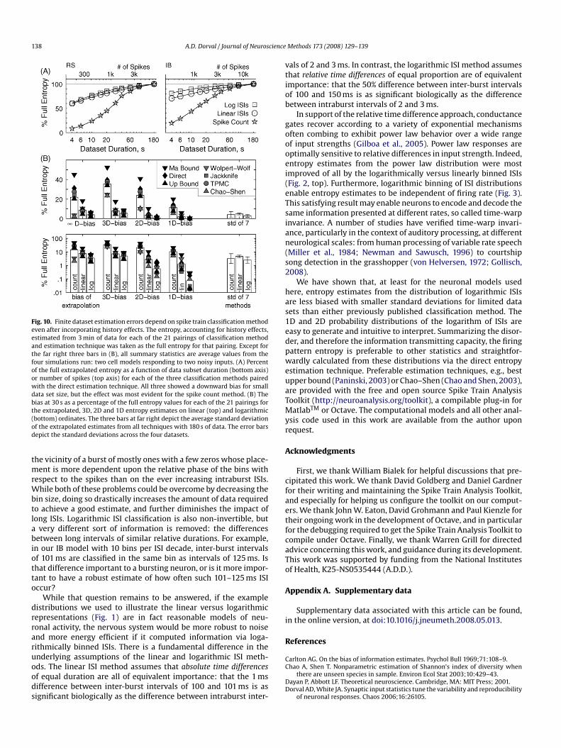
The same high dimensional estimates and their extrapolationswere performed for all 21 method–technique pairings for severaldataset durations (Fig. 10B). Calculated from 30 s of data, the loga-rithmic ISI method had the least bias for each technique in the 1D,2D, 3D and extrapolated cases. In the worst case of 3D distributions,there was only a 5% bias in estimates made from the logarithmicISI method, while the linear ISI and spike count methods yieldedbiases of 8% and 35%, respectively.

A.D. Dorval / Journal of Neuroscience Methods 173 (2008) 129–139 137

Fig. 8. Probability distributions of ISI pairs. The probability of ISI pairs, ISI2 followingISI1, for the RS (left) and IB (right) models in response to the strongly noisy input.Note the logarithmic color bar applies to all four plots. With linear ISI bins (top) theIB behavior is difficult to capture pictorially, because the vast majority of ISI pairsare in the sub-1.5 ms regime (inset). With logarithmic ISI bins (bottom), a conciserepresentation of these disparate cell behaviors can be cleanly presented on axesof the same scale. The RS model fires most often with pairs of ∼10 ms ISIs, varyingsmoothly from 4 to 500 ms. The IB model fires most often with intraburst ISI pairs of∼0.8 ms, varying from 0.4 to 3 ms. The mode to the right represents burst initiationwith an ISI of 10–300 ms and an intraburst ISI which peaks from 0.5–1.0 ms. Themode above the burst mode represents burst completion with a final intraburst ISIpeaking from 1.0 to 1.5 ms and a post-burst ISI of 10–300 ms.

4. Discussion

The firing pattern entropy of a neuron bounds the amountof information that neuron can possibly transmit. Only a fewyears after Shannon’s hallmark information papers (Shannon andWeaver, 1949), physiologists had adapted the theory to analyzeneuronal activity (MacKay and McCulloch, 1952). However, despitemajor advances in entropy estimation techniques (e.g., Treves andPanzeri, 1995; Strong et al., 1998; Paninski, 2003) and substantialinsights information theory has helped illuminate (e.g., Reinagel et

al., 1999; Koch et al., 2006), its application to neuroscience remainsa niche field. While there may be many justifiable reasons for neu-roscientists to avoid information theory, we believe the primaryreason that entropy measures are not more widely used is a percep-tion that information theoretic results are less intuitive and moredifficult to interpret than results from simpler variability statis-tics, including coefficients of variation (CV) or coherences, and adhoc measures such as burst indexes. While these other measurehave their utility, entropy exhibits some preferable characteristicsin many situations. For example, ISI CV is used frequently to assessISI variability (e.g., Dorval and White, 2006), but the results can bemisleading particularly in the presence of strong neural rhythms. Aneuron that generally fires in phase with a rhythm but occasionallyskips cycles could have a very high CV even though its firing patternis extremely predictable. Not fooled by cycle skipping periodicityhowever, comparably low entropy estimates would correctly sig-nify a high degree of predictability. Indeed, information theory wasfounded upon the proof that entropy is an optimal measure of signalvariability (Shannon and Weaver, 1949).

We have presented this work to illustrate the bias and standarddeviation improvements provided to all estimation techniques by

Fig. 9. Examples of finite dataset estimation bias after incorporating history effects.The direct entropy estimation technique was applied to the probability distributionsof words of up to four ISIs or up to 24 time bins – analogous to those described inFig. 5 without history effects for only 1 ISI or 6 time bins – on data subsets of theRS (left) and IB (right) neuronal models responding to highly noisy applied current.Repeated estimates were made for all subsets of fixed duration, and combined toyield a mean and standard deviation for each data subset duration. The mean value ofeach estimation technique with standard deviation is plotted versus the reciprocal ofthe dimension (i.e., one divided by the number of ISIs) for the logarithmic (bottom)and linear (middle) ISI methods, or the firing rate adjusted, reciprocal dimensionequivalent for the spike count method (top). Least-squares fits were extrapolated tozero for all cases and considered the best estimate of the true entropy (grey symbols).

using the probability distribution of the logarithm of ISIs. Intricatecomparisons aside, previous work by others suggested that log-arithmic ISI distributions are easily interpreted for neurons withdisparate spiking patterns (Selinger et al., 2007). In fact, even inresponse to constant suprathreshold inputs, resulting ISIs are more

intuitively described by their logarithm due to the power law rela-tionship between input current and firing rate (Fig. 4). We showedthat this ease of interpretation extends to the 2D distribution of ISIpairs (Fig. 8). The relatively small bias and standard deviation offiring pattern entropy estimates from the logarithmic distributionslend credence to the intuition that the true nature of the firing pat-tern can be garnered more readily from logarithmically, as opposedto linearly, spaced probability distributions.

Of note, while all seven estimation techniques would eventuallyconverge to the same entropy value for enough data, each classifi-cation method will yield different entropy estimates. The binningof spike times is necessarily a lossy compression. After classifica-tion, whether we take the spike counts, linear ISIs or logarithmicISIs, we could not invert them to return to the exact spike times.One question of interest is what information is thrown out by eachclassification method? For the spike count and linear ISI methods,knowledge of the relative spacing of very short ISIs is lost. For our RSmodel with 3.0 ms bins for example, ISIs of 3.1 ms are classified intothe same bin as ISIs of 5.9 ms. For the IB model during a fairly typi-cal burst, all intraburst ISIs are between 0.5 and 1.0 ms, which, withspike count classification and our 0.5 ms bin size, yields strings in

138 A.D. Dorval / Journal of Neuroscience

Fig. 10. Finite dataset estimation errors depend on spike train classification methodeven after incorporating history effects. The entropy, accounting for history effects,estimated from 3 min of data for each of the 21 pairings of classification methodand estimation technique was taken as the full entropy for that pairing. Except forthe far right three bars in (B), all summary statistics are average values from thefour simulations run: two cell models responding to two noisy inputs. (A) Percentof the full extrapolated entropy as a function of data subset duration (bottom axis)or number of spikes (top axis) for each of the three classification methods pairedwith the direct estimation technique. All three showed a downward bias for smalldata set size, but the effect was most evident for the spike count method. (B) Thebias at 30 s as a percentage of the full entropy values for each of the 21 pairings forthe extrapolated, 3D, 2D and 1D entropy estimates on linear (top) and logarithmic(bottom) ordinates. The three bars at far right depict the average standard deviationof the extrapolated estimates from all techniques with 180 s of data. The error barsdepict the standard deviations across the four datasets.

the vicinity of a burst of mostly ones with a few zeros whose place-ment is more dependent upon the relative phase of the bins withrespect to the spikes than on the ever increasing intraburst ISIs.While both of these problems could be overcome by decreasing the

bin size, doing so drastically increases the amount of data requiredto achieve a good estimate, and further diminishes the impact oflong ISIs. Logarithmic ISI classification is also non-invertible, buta very different sort of information is removed: the differencesbetween long intervals of similar relative durations. For example,in our IB model with 10 bins per ISI decade, inter-burst intervalsof 101 ms are classified in the same bin as intervals of 125 ms. Isthat difference important to a bursting neuron, or is it more impor-tant to have a robust estimate of how often such 101–125 ms ISIoccur?

While that question remains to be answered, if the exampledistributions we used to illustrate the linear versus logarithmicrepresentations (Fig. 1) are in fact reasonable models of neu-ronal activity, the nervous system would be more robust to noiseand more energy efficient if it computed information via loga-rithmically binned ISIs. There is a fundamental difference in theunderlying assumptions of the linear and logarithmic ISI meth-ods. The linear ISI method assumes that absolute time differencesof equal duration are all of equivalent importance: that the 1 msdifference between inter-burst intervals of 100 and 101 ms is assignificant biologically as the difference between intraburst inter-

Methods 173 (2008) 129–139

vals of 2 and 3 ms. In contrast, the logarithmic ISI method assumesthat relative time differences of equal proportion are of equivalentimportance: that the 50% difference between inter-burst intervalsof 100 and 150 ms is as significant biologically as the differencebetween intraburst intervals of 2 and 3 ms.

In support of the relative time difference approach, conductancegates recover according to a variety of exponential mechanismsoften combing to exhibit power law behavior over a wide rangeof input strengths (Gilboa et al., 2005). Power law responses areoptimally sensitive to relative differences in input strength. Indeed,entropy estimates from the power law distribution were mostimproved of all by the logarithmically versus linearly binned ISIs(Fig. 2, top). Furthermore, logarithmic binning of ISI distributionsenable entropy estimates to be independent of firing rate (Fig. 3).This satisfying result may enable neurons to encode and decode thesame information presented at different rates, so called time-warpinvariance. A number of studies have verified time-warp invari-ance, particularly in the context of auditory processing, at differentneurological scales: from human processing of variable rate speech(Miller et al., 1984; Newman and Sawusch, 1996) to courtshipsong detection in the grasshopper (von Helversen, 1972; Gollisch,2008).

We have shown that, at least for the neuronal models usedhere, entropy estimates from the distribution of logarithmic ISIsare less biased with smaller standard deviations for limited datasets than either previously published classification method. The1D and 2D probability distributions of the logarithm of ISIs areeasy to generate and intuitive to interpret. Summarizing the disor-der, and therefore the information transmitting capacity, the firingpattern entropy is preferable to other statistics and straightfor-wardly calculated from these distributions via the direct entropyestimation technique. Preferable estimation techniques, e.g., bestupper bound (Paninski, 2003) or Chao–Shen (Chao and Shen, 2003),are provided with the free and open source Spike Train AnalysisToolkit (http://neuroanalysis.org/toolkit), a compilable plug-in forMatlabTM or Octave. The computational models and all other anal-ysis code used in this work are available from the author uponrequest.

Acknowledgments

First, we thank William Bialek for helpful discussions that pre-cipitated this work. We thank David Goldberg and Daniel Gardnerfor their writing and maintaining the Spike Train Analysis Toolkit,

and especially for helping us configure the toolkit on our comput-ers. We thank John W. Eaton, David Grohmann and Paul Kienzle fortheir ongoing work in the development of Octave, and in particularfor the debugging required to get the Spike Train Analysis Toolkit tocompile under Octave. Finally, we thank Warren Grill for directedadvice concerning this work, and guidance during its development.This work was supported by funding from the National Institutesof Health, K25-NS0535444 (A.D.D.).

Appendix A. Supplementary data

Supplementary data associated with this article can be found,in the online version, at doi:10.1016/j.jneumeth.2008.05.013.

References

Carlton AG. On the bias of information estimates. Psychol Bull 1969;71:108–9.Chao A, Shen T. Nonparametric estimation of Shannon’s index of diversity when

there are unseen species in sample. Environ Ecol Stat 2003;10:429–43.Dayan P, Abbott LF. Theoretical neuroscience. Cambridge, MA: MIT Press; 2001.Dorval AD, White JA. Synaptic input statistics tune the variability and reproducibility

of neuronal responses. Chaos 2006;16:26105.

cience

A.D. Dorval / Journal of Neuros

Efron B, Tibshirani RJ. An introduction to the bootstrap. London: Chapman & Hall;1993.

Gilboa G, Chen R, Brenner N. History-dependent multiple-time-scale dynamics in asingle-neuron model. J Neurosci 2005;25:6479–89.

Gollisch T. Time-warp invariant pattern detection with bursting neurons. New J Phys2008;10:15012.

Harris B. The statistical estimation of entropy in the non-parametric case. WisconsinUniversity Madison, Mathematics Research Center; 1975, 318.

Izhikevich EM. Dynamical systems in neuroscience. Cambridge, MA: MIT Press; 2007.Koch K, McLean J, Segev R, Freed MA, Berry MJ, Balasubramanian V, et al. How much

the eye tells the brain. Curr Biol 2006;16:1428–34.Ma S. Calculation of entropy from data motion. J Stat Phys 1981;26:

221–40.MacKay DM, McCulloch WS. The limiting information capacity of a neuronal link.

Bull Math Biophys 1952;14:127–35.Miller G. Note on the bias of information estimates. In: Quastler H, editor. Informa-

tion theory in psychology II-B. Glencoe, IL: Free Press; 1955.Miller J, Grosjean F, Lomanto C. Articulation rate and its variability in spon-

taneous speech: a reanalysis and some implications. Phonetica 1984;41:215–25.

Newman MEJ. Power laws, Pareto distributions and Zipf’s law. Contemp Phys2005;46:323–51.

Newman RS, Sawusch JR. Perceptual normalization for speaking rate: effects of tem-poral distance. Percept Psychophys 1996;58:540–60.

Paninski L. Estimation of entropy and mutual information. Neural Comput2003;15:1191–253.

Methods 173 (2008) 129–139 139

Reinagel P, Godwin D, Sherman SM, Koch C. Encoding of visual information by LGNbursts. J Neurophysiol 1999;81:2558–69.

Rieke F, Warland D, Bialek W. Coding efficiency and information rates in sensoryneurons. Europhys Lett 1993;22:151–6.

Rieke F, Warland D, de Ruyter van Steveninck R, Bialek W. Spikes. MIT Press: Cam-bridge, MA, 1997.

Selinger JV, Kulagina NV, O’Shaughnessy TJ, Ma W, Pancrazio JJ. Methods for char-acterizing interspike intervals and identifying bursts in neuronal activity. JNeurosci Methods 2007;162:64–71.

Shannon CE, Weaver W. The mathematical theory of communication. Urbanan, IL:University of Illinois Press; 1949.

Sigworth F, Sine SM. Data transformations for improved display and fitting of single-channel dwell time histograms. Biophys J 1987;52:1047–54.

Strong SP, Koberle R, de Ruyter van Steveninck RR, Bialek W. Entropy and informationin neural spike trains. Phys Rev Lett 1998;80:197–200.

Treves A, Panzeri S. The upward bias in measures of information derived from limiteddata samples. Neural Comput 1995;7:399–407.

von Helversen D. Gesang es mannchens und lautschema des weibchens bei der feld-heuschrecke Chorthippus biguttulus (Orthoptera, Acrididae). J Comp Physiol ANeuroethol Sens Neural Behav Physiol 1972;81:381–422.

Wolpert DH, Wolf DR. Estimating functions of probability distributions from a finiteset of samples, Part 1: Bayes estimators and the Shannon entropy. arXiv, 1994;arXiv>comp-gas:9403001.

Wolpert DH, Wolf DR. Estimating functions of probability distributions from afinite set of samples. Phys Rev E 1995;52:6841–54 [Erratum in Phys. Rev. E54:6973].