probability distributions as models of data · spurdle, a. empirical 0.2.0 2 univariate models use...
TRANSCRIPT

empirical 0.2.0
Probability Distributionsas
Models of Data
Abby Spurdle
December 3, 2018
Computes continuous (not step) empirical (and nonparametric) probability density, cumula-tive distribution and quantile functions. Supports univariate, multivariate and conditionalprobability distributions, some kernel smoothing features and weighted data (possibly usefulmixed with fuzzy clustering). Can compute multivariate and conditional probabilities. Also,can compute conditional medians, quantiles and modes.
Pre-Intro
This package uses objects, which are also functions, which are also models, which are alsoprobability distributions.
Some functions (constructors) return other functions (models), which can be evaluated.The resulting functions have attributes (which along with their arguments) determine theirreturn values.
This is intermediate between a standard object oriented approach and a functional ap-proach. And I believe that this is the best approach for implementing probability distri-butions, especially nonparametric probability distributions.
Introduction
This package computes what I refer to as empirical models (or empirical probability dis-tributions).
Currently, this includes:
� Continuous empirical probability density functions (EPDFs).
� Continuous empirical cumulative distribution functions (ECDFs).
� Continuous empirical quantile functions (EQFs).
It supports univariate, multivariate and conditional probability distributions.
Currently, univariate models are computed differently to multivariate models:

Spurdle, A. empirical 0.2.0 2
� Univariate models use what I refer to as a quantile approach and compute a seriesof vertices (similar to a standard ECDF) and then use a cubic hermite spline tointerpolate between them. By default, univariate models smooth the data, using alowess style smoother, which I refer to as derandomization.
� Multivariate (and conditional) models use kernel smoothing, which I refer to asrestacking.
EPDFs can be used to compute modes and visualize the shape of probability distributions.ECDFs can be used to compute probabilities and to a lesser extent, visualize the shapetoo. And EQFs can be used to compute medians and quantiles.
Also, we can compute conditional probabilities, medians, quantiles and modes from condi-tional probability distributions, which is similar to regression.
Models may be weighted (possibly useful mixed with fuzzy clustering).
The philosophy behind empirical models, is to model data directly, with as few assumptionsas possible but with some support for robustness.
Important Notes
Currently, this package is experimental.
I’m planning to support categorical variables and random number generation in the future.
There are some problems with univariate models, especially univariate EPDFs. Their firstderivative is not continuous which is particularly noticeable in the outer tails. This caninterfere with mode computation, especially if trying to compute all modal points.
I tried to create a hybrid Kernel-Quantile approach, however, I wasn’t able to get it towork as yet. I will try again later.
The function used to compute modes has had limited testing and there may be additionalproblems.
The current implementation is slow and needs to be optimized, however, this is not acurrent development priority.
Univariate models bind two additional data points by default. Univariate models needunique data points, if they’re not unique then they’re randomized first.
Weighted models have had limited testing too.
Loading the Packages
I’m going to load (and attach) the intoo, empirical, fclust and moments packages:
> library (intoo)
> library (empirical)
> library (fclust)
> library (moments)

Spurdle, A. empirical 0.2.0 3
Preparing the Data
I’m going to use the trees data (from the datasets package) and the unemployment data(from the fclust package):
> data (trees)
> data (unemployment)
And I’m going to convert to metric:
> # -> m
> Height = 0.3048 * trees$Height
> # -> cm
> Girth = 2.54 * trees$Girth
> # -> m ^ 3
> Volume = 0.0283168 * trees$Volume
> #total unemployment rate
> un.rate = unemployment$Total.Rate
> #long term unemployment rate
> lt.rate = unemployment$LongTerm.Share
New matrix objects:
> trees2 = cbind (Height, Girth, Volume)
> unemployment2 = cbind (un.rate, lt.rate)
I’ve provided some more information on the trees2 and unemployment2 data in Appendices.
Univariate Models(and Core Functionality)
Empirical probability density functions are produced by differentiating empirical cumula-tive distribution functions. We can use the epdfuv() function:
> f = epdfuv (Height)
We can print the object directly, however, I recommend using the object.info() functionfrom the intoo package, which at the time of writing, needs some improvement:
> object.info (f)
value, 1
function (x)
{
.epdfuv.eval(x)
}
class, 1
[1] "epdfuv"
%$%derandomize, logical, 1
[1] TRUE
%$%preserve, character, 1
[1] "mean"
%$%bind, logical, 1
[1] TRUE
%$%weighted, logical, 1

Spurdle, A. empirical 0.2.0 4
[1] FALSE
%$%drp, numeric, 1
[1] 0.5
%$%nhood, numeric, 1
[1] 16
%$%n, numeric, 1
[1] 33
%$%x, numeric, 33
[1] 17.66214 18.63810 19.40029 20.01935 20.53220 20.96086 21.32661 21.64504
%$%y, numeric, 33
[1] 0.00000 0.03125 0.06250 0.09375 0.12500 0.15625 0.18750 0.21875
%$%t, numeric, 33
[1] 0.00000000 0.03595790 0.04524868 0.05521615 0.06638265 0.07867495 0.09135053
[8] 0.10485044
%$%w, logical, 1
[1] NA
We can access a single attribute using the attribute operator, also from the intoo package,if required:
> f %$% x
[1] 17.66214 18.63810 19.40029 20.01935 20.53220 20.96086 21.32661 21.64504
[9] 21.92270 22.16340 22.37016 22.54980 22.71111 22.86475 23.01837 23.17535
[17] 23.33649 23.49821 23.65683 23.80772 23.94759 24.07647 24.19646 24.31483
[25] 24.44206 24.59401 24.78957 25.04712 25.39054 25.84517 26.44033 27.22178
[33] 28.26879
We can plot the densities from both density (from the stats package) and epdfuv objects,and then compare them:
> plot (density (Height), ylim=c (0, 0.27) )
> lines (f, col="darkgreen")
18 20 22 24 26 28
0.00
0.05
0.10
0.15
0.20
0.25
density.default(x = Height)
N = 31 Bandwidth = 0.8241
Den
sity
Or using a different smoothing parameter:
> f.75 = epdfuv (Height, drp=0.75)
> plot (f.75)

Spurdle, A. empirical 0.2.0 5
18 20 22 24 26 28
0.00
0.05
0.10
0.15
0.20
0.25
x
y
Reiterating, univariate EPDFs do not have continuous first derivatives which is particularlynoticeable in the outer tails. Another problem is that density estimates in the outer tailsappear too high which implies that the density estimates in other regions are too low.
We can evaluate the object (which is a function), however, this isn’t that useful:
> mean.Height = mean (Height)
> f (mean.Height)
[1] 0.19687
Also, we can compute the empirical mode, using the emode() function:
> mh = emode (f)
> plot (f)
> abline (v=mh, lty=2)
> mh
[1] 24.24218
18 20 22 24 26 28
0.00
0.05
0.10
0.15
0.20
0.25
x
y

Spurdle, A. empirical 0.2.0 6
We can compute vertices for a continuous (not step) empirical cumulative distributionfunction, using the following expression:
P(X ≤ x) = F (x) =
∑i I(x∗i ≤ x)− 1
n− 1
Where I() is 1 if the enclosed expression is true and is 0 if false, n is the number of datapoints and x∗ is a vector of data points.
We can use the ecdfuv() function:
> F.unsmooth = ecdfuv (Height, FALSE)
> F = F.smooth = ecdfuv (Height)
> plot (F.unsmooth)
> lines (F.smooth, col="darkgreen")
18 20 22 24 26 28
0.0
0.2
0.4
0.6
0.8
1.0
x
y
Like epdfuv objects we can evaluate an ecdfuv object.
Let’s say that we want to compute the probability that Height is between 20 and 22 meters:
> F (22) - F (20)
[1] 0.1668722
We can compute an empirical quantile function by inverting the ECDF:
> F.inv.unsmooth = ecdfuv.inverse (Height, FALSE)
> F.inv = F.inv.smooth = ecdfuv.inverse (Height)
> plot (F.inv.unsmooth)
> lines (F.inv.smooth, col="darkgreen")

Spurdle, A. empirical 0.2.0 7
0.0 0.2 0.4 0.6 0.8 1.0
1820
2224
2628
y
x
Like epdfuv and ecdfuv objects we can evaluate an ecdfuv.inverse object.
Let’s say we want to compute the median:
> median = F.inv (0.5)
> median
[1] 23.33547
Note that EQFs are not the exact inverse of ECDFs, because of the way that I’ve imple-mented them.
> F (median)
[1] 0.4995401
Bivariate Models
We can compute bivariate models using the following expressions:
f(x1, x2) =
∑i∈2:(n−1)[g(x∗[i,1],bw1, x1) ∗ g(x∗[i,2],bw2, x2)]
n− 2
Where:
g(x0,bw, x) =2
bwl(
2
bw(x− x0))
And where l() is the restacking PDF (kernel) and bw is the bandwidth.
F (x1, x2) =
∑i∈2:(n−1)[G(x∗[i,1],bw1, x1) ∗G(x∗[i,2],bw2, x2)]
n− 2
Where:
G(x0,bw, x) = L(2
bw(x− x0))
And where L() is the restacking CDF.

Spurdle, A. empirical 0.2.0 8
I’ve excluded the first and last data points, so that the ECDF of the first and last datapoints evaluates to 0 and 1, respectively, for consistency with univariate models.
We can construct bivariate EPDFs and ECDFs using the epdfmv() and ecdfmv() functions:
> f = epdfmv (cbind (Height, Volume) )
> F = ecdfmv (cbind (Height, Volume) )
> plot (f)
x1
x2
0.02
0.02
0.04 0.06
0.08
0.1
0.1
0.12 0.14
0.16
0.0 0.2 0.4 0.6 0.8 1.0
0.0
0.2
0.4
0.6
0.8
1.0
> plot (f, TRUE)
x1x2
> plot (F)

Spurdle, A. empirical 0.2.0 9
x1
x2
0.1 0.2
0.3 0.4
0.5
0.6
0.7
0.8
0.9
0.0 0.2 0.4 0.6 0.8 1.0
0.0
0.2
0.4
0.6
0.8
1.0
> plot (F, TRUE)
x1x2
Or alternatively:
> #plot (f, all=TRUE)
Bivariate models aren’t really useful in themselves except for visualizing the shape of prob-ability distributions. However, we can use bivariate (and multivariate models generally)to compute conditional probability distributions and compute multivariate probabilities,which are discussed later.
Multivariate Models
Bivariate models generalize to multivariate models (with m > 2) easily, however, they’redifficult to visualize:

Spurdle, A. empirical 0.2.0 10
f(x1, x2, ..., xm) =
∑i∈2:(n−1)[g(x∗[i,1],bw1, x1) ∗ g(x∗[i,2],bw2, x2)) ∗ ... ∗ g(x∗[i,m],bwm, xm)]
n− 2
F (x1, x2, ..., xm) =
∑i∈2:(n−1)[G(x∗[i,1],bw1, x1) ∗G(x∗[i,2],bw2, x2)) ∗ ... ∗G(x∗[i,m],bwm, xm)]
n− 2
Where m is the number of variables.
> f = epdfmv (trees2)
> F = ecdfmv (trees2)
Currently, you can’t plot multivariate models (with m > 2).
Conditional Models
We can derive conditional models from multivariate models.
In theory, we can compute a (univariate) conditional ECDF (on one variable) using:
P(X2 ≤ x2 | X1 = x1) = F (x2) =
∫ x2
−∞
fX1,X2(x1, u)
fX1(x1)du
In theory, we can compute a (univariate) conditional ECDF (on two variables) using:
P(X3 ≤ x3 | X1 = x1, X2 = x2) = F (x3) =
∫ x3
−∞
fX1,X2,X3(x1, x2, u)
fX1,X2(x1, x2)du
And this can be generalized to m variables.
We can construct conditional empirical models using the epdfc(), ecdfc() and ecdfc.inverse()functions:
> mean.Girth = mean (Girth)
> cf = epdfc (Volume, c (Height=mean.Height, Girth=mean.Girth), trees2)
> cF = ecdfc (Volume, c (Height=mean.Height, Girth=mean.Girth), trees2)
> cF.inv = ecdfc (Volume, c (Height=mean.Height, Girth=mean.Girth), trees2)
Or alternatively (quoted):
> cf = epdfc ("Volume", c (Height=mean.Height, Girth=mean.Girth), trees2,
is.string=TRUE)
> plot (cf)

Spurdle, A. empirical 0.2.0 11
0.0 0.5 1.0 1.5 2.0 2.5
0.0
0.5
1.0
1.5
x
y
Computing Multivariate Probabilities
We can compute the probability that two random variables are between two pairs of valuesas:
P(a1 ≤ X1 ≤ b1, a2 ≤ X2 ≤ b2) = F (b1, b2)− [F (a1, b2) + F (b1, a2)] + F (a1, a2)
Where a is the lower limits and b is the upper limits.
And for three variables:
P(a1 ≤ X1 ≤ b1, a2 ≤ X2 ≤ b2, a3 ≤ X3 ≤ b3) = F (b1, b2, b3)
− [F (a1, b2, b3) + F (b1, a2, b3) + F (b1, b2, a3)]
+ [F (a1, a2, b3) + F (a1, b2, a3) + F (b1, a2, a3)]
− F (a1, a2, a3)
This can be generalized to four or more variables.
Note that we are computing the probability over a rectangular region. This approach won’twork for nonrectangular regions.
We can use the comb.prob() function, which takes three arguments:
> a = c (20, 20, 0.2)
> b = c (30, 24, 0.8)
> #(using multivariate model from earlier section)
> comb.prob (F, a, b)
[1] 0.03940915
Note that it’s possible to compute multiple regions at once by making a and b matriceswith each row representing one region.

Spurdle, A. empirical 0.2.0 12
Conditional Probabilities and Conditional Statistics
It’s possible to compute conditional probabilities, medians, quantiles or modes from con-ditional models. I’m planning to support conditional means and variances in the nearfuture.
We can compute the conditional probability in the same way as the univariate case:
> #(using conditional model from earlier section)
> #probability that volume is between
> #0.2 and 0.8 cubic meters given mean height
> cF (0.8) - cF (0.2)
[1] 0.614727
We can compute the median or quantile from the quantile function in the same way as theunivariate case:
> #(using conditional model from earlier section)
> #median
> cF.inv (0.5)
[1] 0.2051548
> #lower quartile
> cF.inv (0.25)
[1] 0.01523924
Likewise, we can compute the mode using the emode() function in the same way as theunivariate case.
> #(again, using conditional model from earlier section)
> mh = emode (cf)
> plot (cf)
> abline (v=mh, lty=2)
> mh
[1] 0.6556134
0.0 0.5 1.0 1.5 2.0 2.5
0.0
0.5
1.0
1.5
x
y

Spurdle, A. empirical 0.2.0 13
Conditional probabilities and conditional statistics are similar to regression. It’s possibleto compute conditional probabilities and conditional statistics as functions of one or morevariables, which is even more similar to regression. Currently, there’s no functions in thispackage for this purpose. However, it’s easy to write a module to do this.
Let’s say we want to compute the conditional median and conditional first and third quar-tiles of Volume, as functions of Height:
> x = seq (min (Height), max (Height), length.out=30)
> y = matrix (0, nrow=30, ncol=3)
> for (i in 1:30)
y [i,] = ecdfc.inverse (Volume, c (Height=x [i]), cbind (Height, Volume),
npoints=10)(c (0.5, 0.25, 0.75) )
> plot (Height, Volume)
> lines (x, y [,1])
> lines (x, y [,2], lty=2)
> lines (x, y [,3], lty=2)
●●●
●● ●
●●
●●
●
●●●●
●
●
●●●
●●
●●
●
● ●●
●●
●
20 22 24 26
0.5
1.0
1.5
2.0
Height
Vol
ume
In theory, we should be able to compute the conditional mode in the same way, however,I tried and there are some problems.
Fuzzy Clustering and Weighted Data
Fuzzy clustering computes a membership matrix, with each row corresponding to each datapoint and each column corresponding to each cluster (not variable). Each row representsthe membership of that data point in each cluster as numbers in the interval (0, 1).
The following computes memberships for three clusters and then the weights for the firstcluster:
> w = FKM.gk (unemployment2, k=3, seed=2)$U [,1]
> w = w / sum (w)
Noting that the original dataset contains three variables, however, I’m only using twovariables. Also noting that a weighted scatterplot is given in Appendix 6 (at the end ofthis vignette).

Spurdle, A. empirical 0.2.0 14
However, fuzzy clustering is limited by itself. I use the term “Membership-Weighted DataAnalysis” to refer to the process of modelling the data, weighted according to a membershipmatrix. I’m going to focus on nonparametric probability distributions, however, there aremany ways of modelling such data.
We can compute a weighted bivariate model easily:
> f = epdfmv (unemployment2, w=w)
> plot (f)
x1
x2
0.001
0.002
0.003
0.004
0.0 0.2 0.4 0.6 0.8 1.0
0.0
0.2
0.4
0.6
0.8
1.0
> plot (f, TRUE)
x1x2
Likewise, we can compute a weighted conditional model easily:
> mean.un.rate = mean (un.rate)
> cf = epdfc (lt.rate, c (un.rate=mean.un.rate), unemployment2, w=w)
> plot (cf)
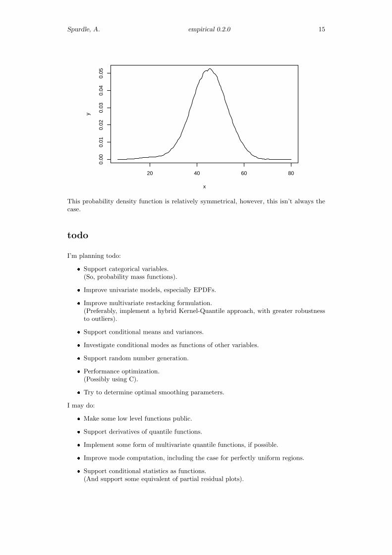
Spurdle, A. empirical 0.2.0 15
20 40 60 80
0.00
0.01
0.02
0.03
0.04
0.05
x
y
This probability density function is relatively symmetrical, however, this isn’t always thecase.
todo
I’m planning todo:
� Support categorical variables.(So, probability mass functions).
� Improve univariate models, especially EPDFs.
� Improve multivariate restacking formulation.(Preferably, implement a hybrid Kernel-Quantile approach, with greater robustnessto outliers).
� Support conditional means and variances.
� Investigate conditional modes as functions of other variables.
� Support random number generation.
� Performance optimization.(Possibly using C).
� Try to determine optimal smoothing parameters.
I may do:
� Make some low level functions public.
� Support derivatives of quantile functions.
� Implement some form of multivariate quantile functions, if possible.
� Improve mode computation, including the case for perfectly uniform regions.
� Support conditional statistics as functions.(And support some equivalent of partial residual plots).

Spurdle, A. empirical 0.2.0 16
� Implement a preserve = “median” (and IQR) feature.
� Implement plot option to shade regions under EPDFs.
� Implement some form of statistical inference.
� In multivariate models, sort the x attribute.(Mainly for consistency with univariate models).

Spurdle, A. empirical 0.2.0 17
Appendix 1:Simplified Bell Curves
> sbcpdf
function (x)
{
y = rep(0, length(x))
I = (x > -1 & x < -0.5)
y[I] = 2 + 4 * x[I] + 2 * x[I]^2
I = (x >= -0.5 & x <= 0.5)
y[I] = 1 - 2 * x[I]^2
I = (x > 0.5 & x < 1)
y[I] = 2 - 4 * x[I] + 2 * x[I]^2
y
}
<bytecode: 0x05b827c8>
<environment: namespace:empirical>
> sbccdf
function (x)
{
y = rep(0, length(x))
I = (x > -1 & x < -0.5)
y[I] = 2/3 + 2 * x[I] + 2 * x[I]^2 + 2/3 * x[I]^3
I = (x >= -0.5 & x <= 0.5)
y[I] = 0.5 + x[I] - 2/3 * x[I]^3
I = (x > 0.5 & x < 1)
y[I] = 1/3 + 2 * x[I] - 2 * x[I]^2 + 2/3 * x[I]^3
I = (x >= 1)
y[I] = 1
y
}
<bytecode: 0x0636c4e8>
<environment: namespace:empirical>
> x = seq (-1, 1, length.out=200)
> y = sbcpdf (x)
> plot (x, y, type="l")
> abline (v=c (-0.5, 0.5), h=c (0.5), lty=2)

Spurdle, A. empirical 0.2.0 18
−1.0 −0.5 0.0 0.5 1.0
0.0
0.2
0.4
0.6
0.8
1.0
x
y
> y = sbccdf (x)
> plot (x, y, type="l")
−1.0 −0.5 0.0 0.5 1.0
0.0
0.2
0.4
0.6
0.8
1.0
x
y

Spurdle, A. empirical 0.2.0 19
Appendix 2:Additional Derandomization Details
The derandomize=TRUE option respaces the data by differencing the data, then trans-forming the differences, then computing a lowess style smoother on the transformed scale(using simplified bell curves) and then reversing the transformations.
There’s n-1 intervals. So, if n is 30 then the number of intervals will be 29. Note that ifbind=TRUE then the n value will higher than the original number of data points.
The smoothness (derandomization) parameter is multiplied by the number of intervals togive the nhood (neighborhood size parameter), so:
nhood = drp ∗ (n− 1)
The nhood parameter gives the number of intervals in the smoothing window, assumingthat the smoothing window does not fall outside the range of observed data. If it does,then the region outside the range is truncated.
If the nhood parameter is provided then the drp parameter is ignored.

Spurdle, A. empirical 0.2.0 20
Appendix 3:Additional Restacking Details
The restacking pdf should be zero centred and symmetrical, with positive densities over theinterval (-1, 1). And the restacking cdf should differentiate to a pdf with these properties.
For each variable, the diff.range is equal to the max value less the min value. So, if themin value 5 and the max value is 15, then the diff.range will be 10.
The smoothness (restacking) parameter is multiplied by the diff.range for each variable, togive a (vector) bandwidth parameter, so:
bwj = rsp ∗ [max(x∗[,j])−min(x∗[,j])]
Like the nhood parameter, the bw parameter defines the width of the smoothing window.
If the bw parameter is provided then the rsp parameter is ignored.

Spurdle, A. empirical 0.2.0 21
Appendix 4:trees2 Data
> object.info (Height)
value, 31
[1] 21.3360 19.8120 19.2024 21.9456 24.6888 25.2984 20.1168 22.8600
class, 1
[1] "numeric"
> object.info (Girth)
value, 31
[1] 21.082 21.844 22.352 26.670 27.178 27.432 27.940 27.940
class, 1
[1] "numeric"
> object.info (Volume)
value, 31
[1] 0.2916630 0.2916630 0.2888314 0.4643955 0.5323558 0.5578410 0.4417421
[8] 0.5153658
class, 1
[1] "numeric"
> summary (trees2)
Height Girth Volume
Min. :19.20 Min. :21.08 Min. :0.2888
1st Qu.:21.95 1st Qu.:28.07 1st Qu.:0.5493
Median :23.16 Median :32.77 Median :0.6853
Mean :23.16 Mean :33.65 Mean :0.8543
3rd Qu.:24.38 3rd Qu.:38.73 3rd Qu.:1.0562
Max. :26.52 Max. :52.32 Max. :2.1804
> skewness (trees2)
Height Girth Volume
-0.3748690 0.5263163 1.0643575
> stripchart (Height, "jitter", pch=1)
Spurdle, A. empirical 0.2.0 22
20 22 24 26
●
●●
●
●
●
●●
●
●
●
●
●●●
●
●
●
●● ●
●
●
●
●
●
●●
●
●
●
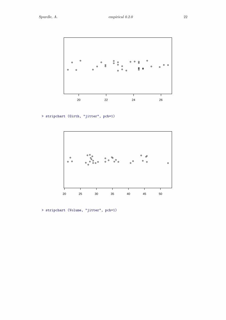
> stripchart (Girth, "jitter", pch=1)
20 25 30 35 40 45 50
●
●
●●
●
●
●
●
●●
●
●
●
●●
●
●●
●●
●
●
●●
●
●
●
●
●
●
●
> stripchart (Volume, "jitter", pch=1)

Spurdle, A. empirical 0.2.0 23
0.5 1.0 1.5 2.0
●
●
●●
●
●
●
●
●
●
●
●
●
●●
●
●
●
●
●
●●
●
●
●
●
●
●
●
●
●
> plot (Height, Girth)
●●●
● ● ●● ● ●● ●●●●
●
● ●●
●● ● ●●
●●
● ●●●●
●
20 22 24 26
2025
3035
4045
50
Height
Gir
th
> plot (Height, Volume)

Spurdle, A. empirical 0.2.0 24
●●●
●● ●
●●
●●
●
●●●●
●
●
●●●
●●
●●
●
● ●●
●●
●
20 22 24 26
0.5
1.0
1.5
2.0
Height
Vol
ume
> plot (Girth, Volume)
● ●●
●●●
●●
●●
●
●● ●●
●
●
●●●
●●
●●
●
●●●
●●
●
20 25 30 35 40 45 50
0.5
1.0
1.5
2.0
Girth
Vol
ume

Spurdle, A. empirical 0.2.0 25
Appendix 5:unemployment2 Data
> object.info (un.rate)
value, 32
[1] 7.1 11.2 6.7 7.6 5.9 12.5 14.4 17.7
class, 1
[1] "numeric"
> object.info (lt.rate)
value, 32
[1] 48.3 56.2 40.5 24.4 48.0 56.8 59.4 49.6
class, 1
[1] "numeric"
> summary (unemployment2)
un.rate lt.rate
Min. : 3.200 Min. :18.60
1st Qu.: 6.925 1st Qu.:28.07
Median : 8.100 Median :42.70
Mean : 9.478 Mean :41.08
3rd Qu.:12.550 3rd Qu.:50.17
Max. :21.600 Max. :67.80
> skewness (unemployment2)
un.rate lt.rate
0.87244093 -0.01797293
> plot (unemployment2)
●
●
●
●
●
●
●
●
●●
●
●
●
●
●
●●
●
●
●
●
●
●
●
●
●
●
●●
●
●
●
5 10 15 20
2030
4050
60
un.rate
lt.ra
te

Spurdle, A. empirical 0.2.0 26
Appendix 6:Weighted Scatter Plot
> s = 1 - w / max (w)
> plot (unemployment2, pch=16, col=rgb (s, s, s) )
●
●
●
●
●
●
●
●
●●
●
●
●
●
●
●●
●
●
●
●
●
●
●
●
●
●
●●
●
●
●
5 10 15 20
2030
4050
60
un.rate
lt.ra
te