Ocean Engineering 120 (2016) 289–297

Contents lists available at ScienceDirect

Ocean Engineering

http://d0029-80

n CorrE-m

sapsis@

journal homepage: www.elsevier.com/locate/oceaneng

Probabilistic response and rare events in Mathieu's equation undercorrelated parametric excitation

Mustafa A. Mohamad, Themistoklis P. Sapsis n

Department of Mechanical Engineering, Massachusetts Institute of Technology, 77 Massachusetts Ave, Cambridge, MA 02139, USA

a r t i c l e i n f o

Article history:Received 30 November 2015Received in revised form2 February 2016Accepted 1 March 2016Available online 25 March 2016

Keywords:Mathieu's equationColored stochastic excitationHeavy-tailsIntermittent instabilitiesRare eventsStochastic roll resonance

x.doi.org/10.1016/j.oceaneng.2016.03.00818/& 2016 Elsevier Ltd. All rights reserved.

esponding author.ail addresses: mmohamad@mit.edu (M.A. Mohmit.edu (T.P. Sapsis).

a b s t r a c t

We derive an analytical approximation to the probability distribution function (pdf) for the response ofMathieu's equation under parametric excitation by a random process with a spectrum peaked at themain resonant frequency, motivated by the problem of large amplitude ship roll resonance in randomseas. The inclusion of random stochastic excitation renders the otherwise straightforward response to asystem undergoing intermittent resonances: randomly occurring large amplitude bursts. Intermittentresonance occurs precisely when the random parametric excitation pushes the system into the instabilityregion, causing an extreme magnitude response. As a result, the statistics are characterized by heavy-tails. We apply a recently developed mathematical technique, the probabilistic decomposition-synthesismethod, to derive an analytical approximation to the non-Gaussian pdf of the response. We illustrate thevalidity of this analytical approximation through comparisons with Monte-Carlo simulations thatdemonstrate our result accurately captures the strong non-Gaussianinty of the response.

& 2016 Elsevier Ltd. All rights reserved.

1. Introduction

Parametrically forced systems arise in many engineering sys-tems and natural phenomena. For such systems, parametric (sub-harmonic) resonance can produce a large response even when theparametric excitation amplitude is small. To investigate these ideas,parametric resonance has been extensively studied using the classicMathieu's equation and the more general Hill's equation,

€xðtÞþðω20þεΩ2 sin ðΩtÞÞxðtÞ ¼ 0; ð1Þ

since it represents the typical response of a systemwhen excited bya time periodic force. When the system's natural frequency and theexcitation frequency are near the ratio ω0 : Ω¼ n : 2, for positiveintegers n, the parametric resonance phenomena is important andwe have regions of instabilities (Fig. 1). The most prominent reso-nance region occurs for n¼1 with the ratio 1:2. Eq. (1) is a simple,deterministic system that is often used to model the typical effect ofparametric excitations that are time periodic or nearly time peri-odic. However, this is only a special case of more typical aperiodictime variations; indeed, in many physical systems, the inducedexcitations are inherently random (e.g. ship motions in randomwater waves (Chai et al., 2015; Lin and Yim, 1995; Kougioumtzoglouand Spanos, 2014; Kreuzer and Sichermann, 2006), modes in

amad),

turbulence (Majda and Lee, 2014; Majda and Tong, 2015; Qi andMajda, 2015), and beam buckling due to random axial and lateralforcing (Abou-Rayan and Nayfeh, 1993; Lin and Cai, 2004). Thisrandomness can significantly alter the system response, and incertain parametric regimes leads to transient instabilities andintermittent bursts of extreme magnitude. These events are directlyconnected with the finite correlation time of the excitation pro-cesses, and therefore cannot be quantified using deterministicanalysis or approximations of the excitation processes by white-noise.

1.1. Motivation

One important parametrically excited system in ocean engi-neering, and our motivating example, is ship rolling in the pre-sence of random seas (Belenky and Sevastianov, 2007; Chai et al.,2015; Lin and Yim, 1995; Kougioumtzoglou and Spanos, 2014;Kreuzer and Sichermann, 2006; Arnold et al., 2004; Fossen andNijmeijer, 2012). The first modern theoretical description ofparametric rolling was given by Paulling and Rosenberg (1959)and the first experimental observation of the phenomenon byPaulling et al. (1975). For ship rolling, the parametric resonancephenomena is a considerable threat to the safety of a vessel.Indeed, ever since the investigation into the post-Panamax C11class cargo ship accident on October 20th, 1998, which was con-firmed to have undergone severe roll motions in head seas duringa storm, causing extensive loss and damage to the vessel (seeFrance et al., 2003 for details), interest in the problem has been

Fig. 1. Ince-Strutt diagram showing the classical resonance tongues (shaded) forparticular combinations of ε and ω2

0=Ω2, for Mathieu's Eq. (1). Transition fre-

quencies at ω20=Ω

2 ¼ ðn=2Þ2. Stability boundaries are computed using Hill's infinitedeterminant approach (Nayfeh and Mook, 1984).

M.A. Mohamad, T.P. Sapsis / Ocean Engineering 120 (2016) 289–297290

renewed. This has lead to developments of important guidelinesand criteria assessing the risk and susceptibility of vessels to rollmotions (American Bureau of Shipping, 2004). As such, the pro-blem of parametric rolling has been an important factor in thepresent debate on the second generation intact stability criteria(see Francescutto, 2015 for the current status of the IMO criteria onrolling).

It is now well understand that large amplitude roll motions canoccur through parametric resonance, even when there are nodirect wave-induced roll moments. This is most prominent in heador following seas, where roll-restoring characteristics can varysignificantly in time compared to still water conditions. When awave crest is amid-ship, stability is reduced as the bow and sternare likely to have emerged, which reduce roll-restoring moments.The effects are most pronounced for wave lengths comparable tothe ship length and increase for steeper waves.

The roll motion of a ship in following or head seas, for smallpitch and heave motions, can be modeled by,

I €ϕðtÞþBð _ϕðtÞÞþΔGZðϕðtÞÞ ¼ FðtÞ; ð2Þwhere ϕðtÞ is the roll angle, I is the inertia term including addedmass, Bð _ϕðtÞÞ is the damping moment, F(t) is a small wave exci-tation term, and ΔGZðϕðtÞÞ is the restoring moment term. Thetime-dependent restoring moments in irregular seas may, some-times, be approximated by (see e.g. Belenky and Sevastianov,2007; Kreuzer and Sichermann, 2006)

ΔGZðϕðtÞÞ ¼ ðαþξðtÞÞϕðtÞ�βϕ3ðtÞ; ð3Þwhere ξðtÞ is the random wave excitation, with a narrowbandedspectrum SξðωÞ around a frequency Ω; thus we expect the para-metric resonance phenomena to be important when the encounterfrequency Ω is roughly twice the natural frequency of rolling. Inaddition, Bð _ϕðtÞÞ is a nonlinear function of the roll velocity. Since ourgoal is to model the leading order probabilistic dynamics that occurdue to the interaction of the random time-dependent restoring termand the vessel's roll angle, we neglect the assumed small nonlinearterms in the restoring and damping moments:

ϕðtÞþ f _ϕðtÞþðαþξðtÞÞϕðtÞ ¼ FðtÞ; ð4Þthis choice is motivated by the fact that stochastic roll resonance, inthis context, is a consequence of the multiplicative excitation term,and not nonlinearities in the restoring or damping terms. However, itis worthwhile to remark on the theoretical nature of Eq. (4); systemnonlinearities are important in accurate models of ship rolling and

play a role in modifying the instability zones (Neves and Rodírguez,2007). The inclusion of the cubic term in the restoring momentwould, for one, impact the underlying shape at the very tail ends ofthe response probability density function by suppressing theirmagnitude. Furthermore, the excitation in roll motion is coupledwith pitch and heave motions, and this requires at least threedegrees of freedom. Despite these remarks, the model in Eq. (4)serves as a useful prototype system for analytical work investigatingthe complex heavy-tailed probabilistic properties of roll resonance inrandom seas; and is motivated by the desire in design to have simpleand accurate analytic predictors of dynamic stability that account forextreme conditions (Spyrou and Papanikolaou, 2000).

This summarizes the basic equation that govern the leading-order ship roll dynamics in the presence of irregular seas. Finally,we note the following: in certain parametric regimes, solutions ofEq. (4) exhibit random periods of large amplitude roll motions(intermittency). It is this parametric regime we are interested ininvestigating here.

1.2. Stochastic generalization of Mathieu's equation

While Mathieu's equation and its variants have been exten-sively analyzed (Champneys, 2009; Nayfeh and Mook, 1984),generalizations incorporating stochasticity are less well under-stood, but have been studied in various contexts (Soong and Gri-goriu, 1993; Lin and Cai, 2004; Poulin and Flierl, 2008; Adams andBloch, 2008; Stratonovich, 1967). A very important dynamicaltransition that occurs in the presence of random parametric for-cing is intermittent resonance; that is, randomly occurring short-lived periods when the system experience parametric resonance.Deterministic models based on some time-averaged property ofthe noise would fail to capture this important dynamical transi-tion, since this is an essentially transient phenomena.

To explore the effects of noise in parametric forcing, motivatedby Section 1.1, we consider the following generalization of Eq. (1):

€xðtÞþ2ζω0 _xðtÞþω20ð1þκðtÞÞxðtÞ ¼ FðtÞ; ð5Þ

where κðtÞ is a narrowbanded random process, F(t) is a broad-banded forcing term of low intensity, e.g. white noise, and ζ is thedamping coefficient. For example, κðtÞ can be thought of asκðtÞ ¼ αðtÞ sin ðΩtÞ, with frequency ratio near one of the resonanceregions and αðtÞ a random process, such that the dominant energyin the spectrum SκðωÞ is concentrated near Ω; in other words, thenoise has a dominant frequency component atΩ. We explain laterin detail the motivation behind this selection, for now we notethat this spectrum follows quite naturally when modeling physicalprocesses, in particular, random seas.

1.3. Perspective

Our goal here is to derive an analytical approximation to theprobability density function (pdf) for the generalized Mathieu'sequation in Eq. (5) when forced parametrically by a correlated randomprocess near the principal resonance region; in particular, we areinterested in the stationary probability distribution of the response inthe regime undergoing intermittency. As mentioned, this is challen-ging since the system exhibits transient resonance, which can beidentified by large amplitude spikes in the time-series of the response;as a result of intermittency, the resulting pdf is non-Gaussian withheavy-tailed characteristics. Recently, there have been efforts toquantify the heavy-tailed statistical structures for systems undergoingintermittent instabilities (Mohamad and Sapsis, 2015; Mohamad et al.;Majda and Tong, 2015; Qi and Majda, 2015). Here, we apply a recentlydeveloped technique designed to approximate the pdf of systemsexhibiting intermittent instabilities: the probabilistic decomposition-synthesis method (Mohamad et al.;Mohamad and Sapsis, 2015). Since

M.A. Mohamad, T.P. Sapsis / Ocean Engineering 120 (2016) 289–297 291

the system we investigate is low-dimensional, with linear dampingand restoring terms, we apply the formulation in Mohamad andSapsis (2015) to approximate the probability measure of the response.This approach provides us with analytical results, taking into accountthe correlated nature of the multiplicative excitation process κðtÞ.

The benefits of this approach are numerous. For systems, such asin Eq. (4), we can derive analytical results for the non-Gaussianresponse pdf, for both the main probability mass and the heavy-tailed structure. For systems where nonlinearities are important, wecan adapt the method and apply the probabilistic decomposition-synthesis method in a computational setting, as described inMohamad et al., for a fast approximation of the response pdf thataccounts for system nonlinearities.

While several methods can be applied to solve for the sta-tionary measure for systems excited by multiplicative noise, forthe case of transient instabilities, as might occur in parametricrolling Eq. (4), they are severely limited in practicality due to theirlarge computational demands and/or limitations in dealing withthe strongly transient nature of intermittent instabilities. Forexample, the Monte-Carlo approach (direct sampling of long timerealizations of the system), while very attractive since it providesthe most accurate results, is a very computationally intensiveprocedure, requiring many realizations for accurately resolved tailstatistics. Another technique is to formulate the associated Fok-ker–Planck–Kolmogorov (FPK) equation for Eq. (5) (Soize, 1994).This can be performed by utilizing shape filtering to approximatethe correlated excitation process. However, using filtered Gaussianwhite noise is prone to introduce significant errors in the tails ofthe response (even small numerical errors in time-series simula-tions of κðtÞ lead to large inaccuracies in the tail statistics of x(t)Majda and Branicki, 2012). In any case, this approach requiressolving a demanding FPK equation (Masud and Bergman, 2005),which also has to be done to high accuracy (tail events haveextremely low probabilities).

Stochastic averaging is another widely used method (Pavliotisand Stuart, 2008); the typical approach here would be to firstderive a set of equations for the slowly varying variables and thento apply the stochastic averaging procedure to arrive at a set of Itōstochastic differential equations for the transformed coordinates.The Fokker–Plank–Kolmogorov equation can then be used to solvefor the response pdf (Lin and Cai, 2004; Floris, 2012). Clearly, thisapproach is not valid in parametric regimes undergoing inter-mittent resonance, since it averages away the time dependentnature of the multiplicative excitation, leading to Gaussian statis-tics, which is decidedly not the case.

1.4. Outline

In Section 2 we formulate the problem and provide the problemstatement; we explain the particular form of the excitation noisestructure and its interaction with the system dynamics in the para-metric regime of interest. Following this discussion, in Section 3, wederive equations that govern the slow dynamics of the problem. Theequations for the slowly varying variables are the starting point of ourapplication of the probabilistic decomposition-synthesis method,which we briefly give an overview in Section 4. In Section 5 we applythe method to derive the analytical formula that approximates the pdfof Mathieu's equation in the parametric regime of interest, and inSection 6 we compare the analytical formula with numerical resultsfrom Monte-Carlo simulations.

2. Problem formulation

We consider the following stochastic generalization ofMathieu's equation:

€xðtÞþ2ζω0 _xðtÞþω20ð1þκðtÞÞxðtÞ ¼ FðtÞ; ð6Þ

where ω0 is the undamped natural frequency of the system, ζ isthe damping coefficient, κðtÞ is a narrowbanded random processaround Ω, and F(t) is an additive broadbanded random excitationterm; we assume that both κðtÞ and F(t) are stationary Gaussianprocesses.

As mentioned, the deterministic form of Mathieu's equation,

€xðtÞþ2ζω0 _xðtÞþω20ð1þα sin ΩtÞxðtÞ ¼ 0; ð7Þ

has unstable solutions depending upon the parametric excitationfrequency Ω and amplitude α parameters. Near Ω=2ω0 ¼ 1=n, forpositive integers n, we have regions of instabilities, with thewidest instability region being for n¼1. Damping has the effect ofraising the instability regions from the Ω=2ω0 axis by 2ð2ζÞ1=n.Therefore, for ζ⪡1 the instability region near n¼1 is of greatestpractical importance (Lin and Cai, 2004; Nayfeh and Mook, 1984).

Furthermore, since we are interested in analyzing the responsepdf in the regime where the system is undergoing intermittentresonance, we assume that κðtÞ is a narrowbanded random processaround the most important resonant region at frequency Ω¼ 2ω0.The approach can be extended if the frequency is detuned, but forsimplicity of the presentation we consider no detuning. In thiscase, intermittent resonance is a possibility since the stochasticprocess κðtÞ may randomly cross into the instability tongue. Inother words, for the regime of interest, on average κðtÞ is in a statesuch that the variance of the response x(t) is associated with thebackground attractor, however with low probability κðtÞ cantransition to a critical regime, producing an intermittentlyunstable response of severe magnitude. Thus, through this regimeswitching, we have randomly occurring periods of large amplituderesponses, which are finite-time instabilities with positive Lyapu-nov exponent; a typical time-series is shown in Fig. 2. The severityof these instabilities depends upon the magnitude of the dampingterm and the amplitude and characteristic time-scale of the mul-tiplicative noise term.

2.1. Excitation process

For concreteness we assume that the excitation process takes acanonical form κðtÞ ¼ αðtÞ sin ð2ω0tÞ, where αðtÞ is a stationaryGaussian process with a non-oscillatory correlation function.Additionally, αðtÞ ¼ 0 and RðτÞ ¼ αðtÞαðtþτÞ ¼ σ2

αe� τ2=2ℓ2α , where ℓα

is the characteristic time-scale of the process and σ2α its variance.

2.2. Problem statement

With these considerations, the problem is to derive anapproximation for the stationary probability distribution for thesystem:

€xðtÞþ2ζω0 _xðtÞþω20ð1þαðtÞ sin ð2ω0tÞÞxðtÞ ¼ FðtÞ; ð8Þ

in the parametric regime undergoing intermittent resonance. Thefinal result is given in Eq. (37).

3. Derivation of the slow dynamics

We proceed by assuming a narrow band response around ω0

and averaging over this fast frequency the governing system Eq. (8).

Fig. 2. Sample realization of Mathieu's equation (middle, Eq. (8) under the parametric excitation term (bottom) and the corresponding averaged variables χ1 and χ2 (top, Eqs.(12) and (13)). The random amplitude forcing term αðtÞ triggers intermittent resonance when it crosses above or below the instability thresholds (dashed lines).

Fig. 3. (Left) Stability diagram for constant (in time) α and for finite damping ζ ¼ 0:1 (red shaded region); (Middle) pdf of the excitation αðtÞ for two different values of σα;(Right) The corresponding analytical pdf of Mathieu's equation according to the decomposition-synthesis method Eq. (37), where we have highlighted the conditionally rareevent component (dashed red) in the full pdf (solid blue), showing that the tails are completely described by rare events, whereas the background dynamics fully determinethe core (the response pdf is shown assuming ℓα ¼ 10:0, other parameters are described in Section 6). (For interpretation of the references to color in this figure caption, thereader is referred to the web version of this paper.)

M.A. Mohamad, T.P. Sapsis / Ocean Engineering 120 (2016) 289–297292

By introducing the coordinate transformation

xðtÞ ¼ χ1ðtÞ cos ðω0tÞþχ2ðtÞ sin ðω0tÞ;_xðtÞ ¼ �ω0χ1ðtÞ sin ðω0tÞþω0χ2ðtÞ cos ðω0tÞ; ð9Þ

in Eq. (8) and using the additional relation _χ 1ðtÞ cos ðω0tÞþ_χ 2ðtÞ sin ðω0tÞ ¼ 0, we obtain the following pair of equations for theslow variables χ1ðtÞ and χ2ðtÞ:

_χ 1 ¼ � 2ζω0 χ1 sin 2ðω0tÞ�12χ2 sin ð2ω0tÞ

� ��

�ω0α2

χ1 sin2ð2ω0tÞ�ω0αχ2 sin 2ðω0tÞ sin ð2ω0tÞ

i� 1ω0

sin ðω0tÞFðtÞ; ð10Þ

_χ 2 ¼�2ζω0

12χ1 sin ð2ω0tÞ�χ2 cos 2ðω0tÞ

� ��ω0α

2χ2 sin 2ð2ω0tÞ:

�ω0αχ1 cos 2ðω0tÞ sin ð2ω0tÞ�þ 1ω0

cos ðω0tÞFðtÞ: ð11Þ

Averaging the deterministic terms in brackets over the fast fre-quency in Eqs. (10) and (11) gives,

_χ 1ðtÞ ¼ � ζ�αðtÞ4

� �ω0χ1ðtÞ�

1ω0

sin ðω0tÞFðtÞ; ð12Þ

_χ 2ðtÞ ¼ � ζþαðtÞ4

� �ω0χ2ðtÞþ

1ω0

cos ðω0tÞFðtÞ: ð13Þ

The equations above for the slow variables provide good pathwiseand statistical agreement with Eq. (8). Furthermore, these equationsmake it clear that an instability is expected when jαðtÞj44ζ(shown in dashed lines in Fig. 2); this instability criterion is nothingmore than the well-known instability condition of the deterministiccase (for fixed in time α), which to leading order is given by:

δ¼ 1=471=2ffiffiffiffiffiffiffiffiffiffiffiffiffiffiffiffiffiffiffiffiffiffiffiffiffiffiα2δ2�4ζ2δ

q, where δ¼ω2

0=Ω2 (see left plot in

Fig. 3).Next, we apply a stochastic averaging procedure to the additive

forcing term, also known as the diffusion approximation (Lin andCai, 2004; Klyatskin, 2005; Sapsis et al., 2011). More specifically, ifthe governing dynamics act on a sufficiently slower time scalethan the memory of the additive stochastic process, then theindependent increment approximation is valid. This is the case ifthe stochastic process F(t) is broadbanded, and leads to the

M.A. Mohamad, T.P. Sapsis / Ocean Engineering 120 (2016) 289–297 293

following set of Itō stochastic differential equations for the slowvariables:

_χ 1ðtÞ ¼ � ζ�αðtÞ4

� �ω0χ1ðtÞþ

ffiffiffiffiffiffiffiffiffiffi2πK

p_W 1ðtÞ; ð14Þ

_χ 2ðtÞ ¼ � ζþαðtÞ4

� �ω0χ2ðtÞþ

ffiffiffiffiffiffiffiffiffiffi2πK

p_W 2ðtÞ; ð15Þ

with K ¼ SF ðω0Þ=2ω20, where SF ðω0Þ is the spectral density of the

additive excitation F(t) at frequency ω0, and _W 1 and _W 2 areindependent white noise processes of unit intensity (Lin and Cai,2004). The slowly varying variables, after averaging the forcingterm, transform to two decoupled stochastic differential equations.Eqs. (14) and (15) are a good statistical approximation to the ori-ginal system Eq. (8) (but provide poor pathwise agreement).

We emphasize that the broadband hypothesis for the additivestochastic process is a convenient setup that leads to the derivedwhite-noise formulation. However, the analysis and results thatfollow do not require the white-noise formulation and are directlyapplicable for the general case of an (non white-noise) additivestochastic forcing. Such a case could be, for example, an additivenarrowbanded forcing term with spectral content distributedaround ω0.

4. The probabilistic decomposition-synthesis method

The analysis in Section 2 provides the dynamics of the slowvariables and reveals the interaction of the parametric excitationprocess αðtÞ with the slow variables. Starting from these equationswe can apply the probabilistic decomposition-synthesis method toanalytically approximate the stationary measure of χðtÞ. To be self-contained, we provide a very brief overview of the probabilisticdecomposition-synthesis method adapted to the current problem;further details can be found in Mohamad and Sapsis (2015) and adetailed description of the method in a general context in Moha-mad et al.

The main idea of the method is to decompose the systemresponse as:

xðtÞ ¼ xbðtÞþxrðtÞ; ð16Þwhere xr is the solution when a rare event due to an instabilityoccurs and xb is the stochastic response otherwise, i.e. the back-ground dynamics. To be more specific xr will be the response of thesystem when the following two conditions are satisfied: (i)JxJ4ζ, where ζ is the extreme event threshold with respect to achosen norm J � J , and (ii) the parametric excitation obtainsvalues that lead to an instability, i.e. αðtÞARe, where Re describesthe critical region of values for αðtÞ that induce an instability.

Together with this decomposition into rare events and thestochastic background, we also adopt the following assumptions:

1. The existence of intermittent events has negligible effect on thestatistical characteristics of the stochastic attractor and can beignored when analyzing the background state xb.

2. Rare events are statistically independent from each other.

With this setup we can analyze the two states separately andprobabilistically synthesize the information obtained from thisanalysis. This is completed using a total probability argument toobtain the statistics for an arbitrary quantity of interest q by

ρðqÞ ¼ ρðqj JxJ4ζ;αAReÞPrþρðqjx¼ xbÞð1�PrÞ: ð17ÞIn this paper, the quantity of interest is the system response x. Thefirst term expresses the contribution of rare events due toinstabilities and is the heavy-tailed portion of the distribution for q

and the second term expresses the contribution of the backgroundstate, which contributes the main probability mass in the pdf for q.Moreover, Pr �PðJxJ4ζ;αAReÞ is the total probability of a rareevent, which is defined as the ratio between the time the systemspends in rare event responses over the total time. Note that thetemporal duration of rare transitions also includes a decay orrelaxation phase to the background attractor, where the instabilityis no longer active but the system response still has importantmagnitude.

5. The probability distribution for the response

Here we apply the various steps of the probabilisticdecomposition-synthesis method to derive analytical results thatapproximate the heavy-tailed distribution of the response for thesystem in Eq. (8). In particular, we apply the method directly onthe slow variables, since the fast frequency we averaged over isinconsequential in the pdf of the response.

Firstly, because αðtÞ is a zero mean process both χ1ðtÞ and χ2ðtÞfollow the same probability distribution. Consider the followingequation that represents the slowly varying variables:

_χ ðtÞ ¼ � ζ�αðtÞ4

� �ω0χðtÞþ

ffiffiffiffiffiffiffiffiffiffi2πK

p_W ðtÞ ð18Þ

We write Eq. (18) as

_χ ðtÞ ¼ �γðtÞχðtÞþσF_W ðtÞ; ð19Þ

where σF ¼ffiffiffiffiffiffiffiffiffiffi2πK

pand γðtÞ ¼ ζω0�ω0αðtÞ=4 is a Gaussian process

with mean ζω0 and standard deviation σαω0=4. Eq. (19) will bethe starting point for the application of the decomposition-synthesis method.

5.1. Decomposition and the instability region

Eq. (19) makes it clear that intermittency is due to the para-metric forcing term γðtÞ switching signs from positive to negativevalues. This sign switching causes χðtÞ to transition from its regularresponse to a domain where the likelihood of an instability is high.This switching in γðtÞ is the mechanism behind instabilities in thevariable χðtÞ. Therefore, we define the instability region as

Re≔fγðtÞjγðtÞo0g: ð20ÞIn addition, for convenience, we define an instability threshold byη≔4ζ=σα, the ratio of the mean over the standard deviation of theprocess γ.

5.2. Conditional distribution of the background dynamics

In the background state Rce, by definition, we have no rare

events. We can approximate the background dynamics by repla-cing γðtÞ with its average value in this regime. The conditionalaverage of γðtÞ in Rc

e is

γ j γ40 ¼ ζω0þσαω0

4ϕðηÞΦðηÞ; ð21Þ

where ϕð�Þ is the normal probability density function and Φð�Þ isthe normal cumulative distribution function; thus the backgrounddynamics is described by the Ornstein–Uhlenbeck process:

_χ ðtÞ ¼ �γ j γ40χðtÞþσF_W ðtÞ: ð22Þ

Now the dynamics are globally stable in Rce and we can directly

obtain the stationary distribution for Eq. (22):

ρχ ðχ jRceÞ ¼

ffiffiffiffiffiffiffiffiffiffiffiffiffiffiγ j γ40

πσ2F

sexp �γ j γ40

σ2F

χ2

!; ð23Þ

M.A. Mohamad, T.P. Sapsis / Ocean Engineering 120 (2016) 289–297294

which is Gaussian distributed. To formulate our result in terms of thesystem variable x, we refer to the narrowbanded approximationmade when averaging the governing system Eq. (8). This gives,approximately, x¼ χ cos φ; where φ is a uniform random variabledistributed between 0 and 2π. The probability density function forz¼ cos φ is given by ρzðzÞ ¼ 1=ðπ

ffiffiffiffiffiffiffiffiffiffiffiffi1�z2

pÞ, zA ½�1;1�. To avoid

additional integrations for the computation of the pdf, we approx-imate the distribution for z by ρzðzÞ ¼ 1

2ðδðzþ1Þþδðz�1ÞÞ. This givesthe following approximation for the background statistics:

ρðxjRceÞ ¼ ρχ ðxjRc

eÞ ¼ffiffiffiffiffiffiffiffiffiffiffiffiffiffiγ j γ40

πσ2F

sexp �γ j γ40

σ2F

x2 !

: ð24Þ

Therefore, the conditional distribution of the background dynamics isGaussian distributed.

5.3. Conditional distribution of rare events

Here we derive the conditional distribution of the responsewhen an instability occurs. We characterize localized instabilitiesby a growth phase, corresponding directly to γðtÞo0, and arelaxation phase that brings the system back to the backgroundstate; both phases follow the same distribution (Mohamad andSapsis, 2015). Additionally, during the occurrence of an instabilitywe neglect additive excitation and damping, and approximate themagnitude of the envelope as ξ� jχ j Cξ0eΛTγo 0 , where ξ0 is themagnitude of the position's envelope, jχ0 j right before theinstability has begun to emerge, Λ is a random variable thatrepresents the Lyapunov exponent, and Tγo0 is the random lengthof time that the process γ spends below the zero level.

We first determine the statistical characteristics of Λ and Tγo0

(which we assume are independent). By substituting the repre-sentation ξ� jχ jC jχ0 jeΛTγo 0 into Eq. (19) we obtain Λ¼ �γ sothat

ρΛðλÞ ¼Pð�γ j γo0Þ ¼ 4σαω0ð1�ΦðηÞÞϕ 4

λþζω0

σαω0

� �: ð25Þ

The distribution of the duration of time the process γðtÞ spendsbelow an arbitrary threshold level η is not in general available.However, one can show that the asymptotic expression in the limitof rare crossings, η-1, is (Rice, 1958)

ρTγo 0ðtÞ ¼ πt

2T2e

�πt2=4T2

; ð26Þ

and in our case this is a good approximation since we assume thatinstabilities are rare events. In Eq. (26) T represents the averagelength of an instability, which for a Gaussian process is given bythe ratio between the probability of γo0 and the average numberof downcrossings of the zero level per unit time N�

γ ð0Þ by γ (Rice,1958)

T ¼Pðγo0ÞN�γ ð0Þ ¼ 1�ΦðηÞ

12π

ffiffiffiffiffiffiffiffiffiffiffiffiffiffiffiffi�R″

αð0Þq

expð�η2=2Þ; ð27Þ

where we have used Rice's formula for the expected number ofupcrossings (Blake and Lindsey, 1973) and RαðτÞ is the correlationfunction of αðtÞ and R″

αð0Þ is the second derivative of the correla-tion function evaluated at τ¼ 0.

With these results we can determine the distribution of ξ in Re;the derived distribution is given by:

ρðξjξ0;αAReÞ ¼ 1ξ

Z 1

0

1yρΛðyÞρT

log ðξ=ξ0Þy

� �dy; ξ4ξ0: ð28Þ

Substituting in Eqs. (25) and (26) gives,

ρðξjξ0;αAReÞ ¼2π log ðξ=ξ0Þ

σαω0T2ð1�ΦðηÞÞξ

Z 1

0

1y2ϕ 4

yþζω0

σαω0

� �

exp � π

4T2y2

log ðξ=ξ0Þ2 !

dy; ξ4ξ0: ð29Þ

The variable ξ0 corresponds to the magnitude of the backgroundstate xb before an instability occurs. Since, the background state isa narrowbanded Gaussian process, the magnitude of the envelopeξ0 can be modeled as a Rayleigh distribution (see Langley, 1986)with scale parameter equal to the standard deviation of theGaussian process Eq. (24).

Note, however, that in Eq. (17) we are interested in the condi-tional statistics of events caused by instabilities which also haveimportant magnitude. As described in Mohamad and Sapsis(2015), if the envelope's magnitude when an instability occurs issmall, then even though we have an instability we do not neces-sarily have a rare event, i.e. a response that is distinguishable fromthe typical background state response. This requires us to considerbackground states ξ0, which are sufficiently large to result in a rareevent JxJ4ζ. To this end, we consider only background statessuch that ξ04ζ ¼ σF=

ffiffiffiffiffiffiffiffiffiffiffiffiffiffiffiffiffi2γ j γ40

p, i.e. we consider extreme respon-

ses with magnitude at least one standard deviation of the back-ground statistics when an instability also occurs. We emphasizethat the exact choice for ζ plays little role on the approximationproperties of the derived analytical expression. This requirementgives the final distribution for ξ0,

ρξ0 ðξ0 jξ04ζÞ ¼ 2γ j γ40

σ2F

ðξ0�ζÞ exp �γ j γ40

σ2F

ðξ0�ζÞ2 !

; ξ04ζ:

ð30ÞUsing Eq. (30) in Eq. (29) we obtain

ρðξjξ4ζ;αAReÞ ¼Zρðξjξ0;αAReÞρξ0 ðξ0 jξ04ζÞ dξ0: ð31Þ

In the last step, we transform the envelope representation back tothe real variable x through the same narrowbanded argumentused in Section 5.2 for the background state distribution; this givesthe final result for the distribution of the rare event regime:

ρðxj JxJ4ζ;αAReÞC12

Zρð xj jjξ0;αAReÞρξ0 ðξ0 jξ04ζÞ dξ0; ð32Þ

¼ffiffiffiffiffiffi2π

pγ j γ40

σ2Fσαω0 T

2ð1�ΦðηÞÞ

Z j xj

ζ

Z 1

0

log ðjxj=ξ0Þy2ðjxj=ðξ0�ζÞÞ

exp �8ðyþζω0Þ2σ2αω2

0

� π

4T2y2

log ðjxj=ξ0Þ2�γ j γ40

σ2F

ðξ0�ζÞ2!

dy dξ0:

5.4. Probability of rare events

Next we determine the total probability of rare events, that isthe ratio of time that the system response spends in rare transi-tions over the total time, which we denote by Pr . This quantity canbe computed by analyzing the duration of transitions into Re, i.e.the duration of instabilities, but also including the time it takes forthe response to return to the background attractor.

Consider a representative extreme event with an averagegrowth rate Λþ and decay rate Λ � . During the growth phase thedynamics are approximated by:

ξp ¼ ξ0 expðΛ þ Tγo0Þ; ð33Þ

where Tγo0 is the duration of the growth event and ξp is the peakvalue of the response. Similarly, over the decay phase:

ξ0 ¼ ξp expð�Λ� TdecayÞ: ð34Þ

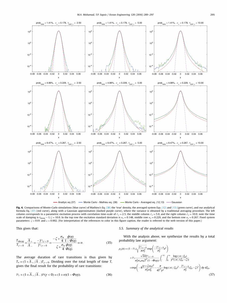
Fig. 4. Comparisons of Monte-Carlo simulations (blue curve) of Mathieu's Eq. (38) the ‘true’ density, the averaged system Eqs. (12) and (13) (green curve), and our analyticalformula Eq. (37) (red curve), along with a Gaussian approximation (dashed purple curve), where the variance is obtained by a traditional averaging procedure. The leftcolumn corresponds to a parametric excitation process with correlation time-scale of ℓα ¼ 2:5, the middle column ℓα ¼ 5:0, and the right column ℓα ¼ 10:0; note the timescale of damping is tdamp � 1=ζ¼ 10:0. In the top row the excitation standard deviation is σα ¼ 0:148, middle row σα ¼ 0:229, and the bottom row σα ¼ 0:267. Fixed systemparameters: ζ¼ 0:01 and ν¼ 0:002. (For interpretation of the references to color in this figure caption, the reader is referred to the web version of this paper.)

M.A. Mohamad, T.P. Sapsis / Ocean Engineering 120 (2016) 289–297 295

This gives that:

Tdecay

Tγo0¼Λ þΛ �

¼ �γ j γo0

γ j γ40¼

�ζþσα4

ϕðηÞ1�ΦðηÞ

ζþσα4ϕðηÞΦðηÞ

� υ: ð35Þ

The average duration of rare transitions is thus given byTe ¼ ð1þΛ þ =Λ � ÞTγo0. Dividing over the total length of time T,gives the final result for the probability of rare transitions:

PrC ð1þΛþ =Λ� ÞPðγo0Þ ¼ ð1þυÞð1�ΦðηÞÞ: ð36Þ

5.5. Summary of the analytical results

With the analysis above, we synthesize the results by a totalprobability law argument:

ρxðxÞ ¼ ð1�PrÞffiffiffiffiffiffiffiffiffiffiffiffiffiffiγ j γ40

πσ2F

sexp

�γ j γ40

σ2F

x2 !

þPr

ffiffiffiffiffiffi2π

pγ j γ40

σ2Fσαω0T

2ð1�ΦðηÞÞ

Z j xj

ζ

Z 1

0

log ðjxj=ξ0Þy2ðj xj=ðξ0�ζÞÞ

�exp �8ðyþζω0Þ2σ2αω2

0

� π

4T2y2log ðjxj=ξ0Þ2�

γ j γ40

σ2F

ðξ0�ζÞ2 !

dy dξ0;

ð37Þ

M.A. Mohamad, T.P. Sapsis / Ocean Engineering 120 (2016) 289–297296

where the integral is zero for jxjoζ. Note that σ2F ¼ πSF ðω0Þ=ω2

0for the case of a broadbanded additive excitation and σ2

F ¼ ν2=2ω20

for the case of a white noise additive excitation with intensity ν(i.e. FðtÞ ¼ ν _W ðtÞ).

We emphasize that Eq. (37) is a heavy-tailed and symmetricprobability measure (non-negative and integrates to one). In Fig. 3we present the stability diagram for constant (in time) α and forfinite damping ζ ¼ 0:1 (red shaded region in the left plot). For thecase where Ω¼ 2ω0 we apply a random amplitude parametricexcitation with pdf for αðtÞ shown in the middle plot for two dif-ferent values of σα. (Note that there are other important factorsthat play an important role in the form of the tails, not captured inthe stability diagram or the pdf of αðtÞ, such as the correlationfunction of the process αðtÞ.) In the right plot, the correspondingresponse pdf as computed through Eq. (37) for the same twovalues of σα are shown, illustrating the heavy-tailed component,due to the conditionally rare dynamics, and the core of the pdf,due to the conditionally background state. It is clear that transientinstabilities, rare responses, fully determine the tails of the pdf,while the background dynamics specify the core of the distribu-tion, but contribute essentially zero probability to the tails.

6. Comparisons with Monte-Carlo simulations

To illustrate the accuracy of our approximation Eq. (37), wecompare the analytical formula obtained via the probabilistic-decomposition technique with direct Monte-Carlo simulations ofthe original system. To perform comparisons we use a unit whitenoise _W ðtÞ process with intensity ν for the additive forcing term F(t), and furthermore non-dimensionalize time by ω0 in Eq. (8) sothat,

€xðtÞþ2ζ _xðtÞþð1þαðtÞ sin 2tÞxðtÞ ¼ ν _W ðtÞ: ð38ÞThus, for this additive forcing we have σ2

F ¼ ν2=2ω20.

To perform the Monte-Carlo simulations, we compute 3000realization of the above equation using the Euler–Maruyamamethod with time step dt ¼ 5� 10�3 from t¼0 to t¼5500 anddiscard the first 500 time units, to ensure a statistical steady state.Moreover, we generate realizations of the stochastic process αðtÞdirectly from the autocorrelation function by a statistically exactand efficient method using the circulant embedding technique(Kroese and Botev, 2014).

In Fig. 4 we show nine cases of varying intermittency levels. Wefix the system parameters ζ ¼ 0:1 and ν¼ 0:002. In the figure, weshow the response pdf for three different correlation times of ℓα¼ 2:5;5:0;10:0 and for three different values of the standarddeviation of the parametric excitation αðtÞ: σα ¼ 0:178;0:229;0:267; For the least intermittent case the standard deviation of αðtÞis σα ¼ 0:178 so that rare event transitions occur with probabilityPr ¼ 0:0141, for σα ¼ 0:229 with probability Pr ¼ 0:0488, and forthe most intermittent case Pr ¼ 0:0847.

Overall, the results presented, along with additional numericalcomparisons, show good quantitative agreement for both the tailsand the core of the distribution between our analytical formula inEq. (37) and the ‘true’ density from Monte-Carlo simulations;indeed, the quantitative agreement between our formula and theactual density is found to be robust across a range of parametersthat satisfy the assumptions. We observe our result performs betterwith the averaged system, onwhich we directly derived the density,than the original system for cases with larger correlation times ℓαand larger variance σ2

α in the parametric excitation process αðtÞ; thisbehavior is expected since averaging introduces well known errorsthat increase for more intermittent regimes, because the instabil-ities in such cases lead to even larger amplitude responses. More-over, we observe that even in extremely intermittent regimes,

where our assumptions start to be violated, namely the statisticalindependence of rare events, our analytical formula is still able tocapture the asymptotic behavior of the tails.

Clearly, the results show that the response pdf is far fromGaussian, and highlight the non-Gaussianity of roll motions duringparametric resonance. Despite the simplicity and theoretical nat-ure of our model, the overall characteristics and shape of thedistribution is the same as that observed in Monte-Carlo simula-tions using advanced hydrodynamic codes with three degrees offreedom that account for coupled pitch, heave, and roll motions(Belenky et al., 2011; Belenky and Weems, 2012).

7. Conclusions

In this work we derived an analytical approximation to theheavy-tailed stationary measure of Mathieu's equation underparametric excitation by a correlated stochastic process in aregime undergoing intermittent parametric resonances. Wederived the formula for the case when the spectrum of the noise ispeaked at the main resonant frequency. To derive the pdf for theresponse we averaged the governing equation over the fast fre-quency to arrive at a set of parametrically excited processes thatgovern the slow dynamics. We then applied the probabilisticdecomposition-synthesis method to the slow variables. Wedemonstrated the accuracy of the final formula for the pdf throughdirect comparisons with Monte-Carlo results for a range para-meters that influence the rare event transition probability leveland severity of the resonance phenomena; the analytical formulashowed excellent quantitative agreement with results fromnumerical simulations across a wide range of intermittency levels.The approach is also directly applicable for the determination ofthe local maxima of the response.

The presented analysis paves the way for the analytical treat-ment of more realistic ship roll models. Future work includes theinclusion of nonlinear terms, in particular, softening nonlinearityin the restoring force, which would modify the statistical char-acteristics of the tails. Such a problem could be considered throughthe current framework by analytical modeling of the nonlinearterms during the rare transitions, in combination with appropriatenonlinear closures for the background stochastic attractor. Addi-tional work will include application of the decomposition-synthesis method in a data-driven context using models contain-ing model error to derive tail estimates.

Acknowledgments

This research has been partially supported by the Office ofNaval Research (ONR) Grant ONR N00014-14-1-0520 and theNaval Engineering Education Center (NEEC) Grant 3002883706.We thank Dr. Vadim Belenky for numerous stimulating discus-sions. We are also grateful to Profs. Francescutto, Neves, andVassalos for the invitation to prepare a manuscript for this specialissue of Ocean Engineering Journal on Stability and Safety of Shipsand Ocean Vehicles.

References

Abou-Rayan, A., Nayfeh, A., 1993. Stochastic response of a buckled beam to externaland parametric random excitations. In: AIAA/ASME/ASCE/AHS/ASC 34thStructures, Structural Dynamics, and Materials Conference, vol. 1, pp. 1030–1040.

Adams, F.C., Bloch, A.M., 2008. Hill' equation with random forcing terms. SIAM J.Appl. Math. 68 (4), 947–980.

M.A. Mohamad, T.P. Sapsis / Ocean Engineering 120 (2016) 289–297 297

American Bureau of Shipping, 2004. Guide for the Assessment of Parametric RollResonance in the Design of Container Carriers (2004 – original publication,2008 – amendment).

Arnold, L., Chueshov, I., Ochs, G., 2004. Stability and capsizing of ships in randomsea—a survey. Nonlinear Dyn. 36, 135–179.

Belenky, V.L., Sevastianov, N.B., 2007. Stability and Safety of Ships: Risk of Capsiz-ing. The Society of Naval Architects and Marine Engineers, Jersey City, NJ.

Belenky, V., Weems, K., Lin, W.-M., Paulling, J., 2011. Probabilistic analysis of rollparametric resonance in head seas. In: Almeida Santos Neves, M., Belenky, V.L.,de Kat, J.O. Spyrou, K., Umeda, N. (Eds.), Contemporary Ideas on Ship Stabilityand Capsizing in Waves, Fluid Mechanics and Its Applications, vol. 97. Springer,Netherlands, 2011, pp. 555–569.

Belenky, V., Weems, K., 2012. Probabilistic properties of parametric roll. In: Fossen,T.I., Nijmeijer, H. (Eds.), Parametric Resonance in Dynamical Systems. Springer,New York, pp. 129–145.

Blake, I.F., Lindsey, W.C., 1973. Level-crossing problems for random processes. IEEETrans. Inf. Theory 19, 295–315.

Chai, W., Naess, A., Leira, B.J., 2015. Stochastic dynamic analysis and reliability of avessel rolling in random beam seas. J. Ship Res. 59 (2), 113–131.

Champneys, A., 2009. Dynamics of parametric excitation. In: Meyers, R.A. (Ed.),Encyclopedia of Complexity and Systems Science. Springer, New York,pp. 2323–2345.

Floris, C., 2012. Stochastic stability of damped Mathieu oscillator parametricallyexcited by a Gaussian noise. Math. Prob. Eng. 2012, 1–18.

Fossen, T.I., Nijmeijer, H., 2012. Parametric Resonance in Dynamical Systems.Springer, New York, NY.

France, W., Levadou, M., Treakle, T., Paulling, J., Michel, R., Moore, C., 2003. Aninvestigation of head-sea parametric rolling and its influence on containerlashing systems. Mar. Technol. 40 (1), 1–19.

Francescutto, A., 2015. Intact stability of ships past present and future. In: Pro-ceedings of the 12th International Conference on Stability of Ships and OceanVehicles, Glasgow, U.K., pp. 1199–1209.

Klyatskin, V.I., 2005. Stochastic Equations through the Eye of the Physicist. ElsevierPublishing Company, Amsterdam, The Netherlands.

Kougioumtzoglou, I.A., Spanos, P.D., 2014. Stochastic response analysis of the soft-ening Duffing oscillator and ship capsizing probability determination via anumerical path integral approach. Probab. Eng. Mech. 35, 67–74.

Kreuzer, E., Sichermann, W., 2006. The effect of sea irregularities on ship rolling.Comput. Sci. Eng. (May/June), 26–34.

Kroese, D.P., Botev, Z.I., 2014. Spatial process generation. In: V. Schmidt (Ed.). Lec-tures on Stochastic Geometry, Spatial Statistics and Random Fields, Volume II:Analysis, Modeling and Simulation of Complex Structures, Springer-Verlag,Berlin.

Langley, R., 1986. On various definitions of the envelope of a random process. J.Sound Vib. 105 (3), 503–512.

Lin, Y.K., Cai, G.Q., 2004. Probabilistic structural dynamics: advanced theory andapplications. McGraw-Hill, New York, c2004.

Lin, H., Yim, S.C., 1995. Chaotic roll motion and capsize of ships under periodicexcitation with random noise. Appl. Ocean Res. 17 (3), 185–204.

Majda, A.J., Branicki, M., 2012. Lessons in uncertainty quantification for turbulentdynamical systems. Discret. Contin. Dyn. Syst. 32, 3133–3221.

Majda, A.J., Lee, Y., 2014. Conceptual dynamical models for turbulence. Proc. Natl.Acad. Sci. U. S. A. 111 (18), 6548–6553.

Majda, A., Tong, X., 2015. Intermittency in Turbulent Diffusion Models with a MeanGradient. Nonlinearity 28, 11.

Masud, A., Bergman, L.A., 2005. Solution of the four dimensional Fokker–Planckequation: still a challenge. In: International Conference on Structural Safety andReliability, vol. 2005, pp. 1911–1916.

Mohamad, M.A., Sapsis, T.P., 2015. Probabilistic description of extreme events inintermittently unstable systems excited by correlated stochastic processes.SIAM ASA J. Uncertain. Quantif. 3, 709–736.

Mohamad, M.A., Cousins, W., Sapsis, T.P., A probabilistic decomposition-synthesismethod for the quantification of rare events due to internal instabilities, sub-mitted for publication.

Nayfeh, A.H., Mook, D.T., 1984. Nonlinear Oscillations. Wiley-Interscience, NewYork.

Neves, M.A., Rodírguez, C.A., 2007. Influence of non-linearities on the limits ofstability of ships rolling in head seas. Ocean Eng. 34 (11–12), 1618–1630.

Paulling, J.R., Rosenberg, R.M., 1959. On unstable ship motions resulting fromnonlinear coupling. J. Ship Res. 3 (1), 36–46.

Paulling, J., Oakley, O.H., Wood, P., Ship, 1975. Capsizing in heavy seas: the corre-lation of theory and experiments. In: Proceedings of the 1st InternationalConference on Stability of Ships and Ocean Vehicles, Glasgow.

Pavliotis, Grigorios A., Stuart., A.M., 2008. Multiscale Methods: Averaging AndHomogenization. Springer, New York, c2008..

Poulin, F.J., Flierl, G.R., 2008. The stochastic Mathieu's equation. Proceedings of theRoyal Society of London A: Mathematical Physical and Engineering Sciences464 (2095), 1885–1904.

Qi, D., Majda, A., 2015. Predicting fat-tailed intermittent probability distributions inpassive scalar turbulence with imperfect models through empirical informationtheory. accepted. Comm. Math. Sci.

Rice, S.O., 1958. Distribution of the duration of fades in radio transmission: Gaus-sian noise model. Bell Syst. Tech. J. 37, 581–635.

Sapsis, T.P., Vakakis, A.F., Bergman, L.A., 2011. Effect of stochasticity on targetedenergy transfer from a linear medium to a strongly nonlinear attachment.Probab. Eng. Mech. 26, 119–133.

Soize, C., 1994. The Fokker-Planck equation for stochastic dynamical systems and itsexplicit steady state solutions. World Scientific Publishing Co., Inc, River Edge,NJ.

Soong, T.T., Grigoriu, M., 1993. Random vibration of mechanical and structuralsystems. PTR Prentice Hall, Englewood Cliffs, N.J., c1993.

Spyrou, K., Papanikolaou, A., 2000. Ship design for dynamic stability. In: Proceed-ings of the 7th International Marine Design Conference (IMDC2000), November1999, Kyongju, Korea, pp. 167–178.

Stratonovich, R.L., 1967. Mathematics and its Applications. Topics in the Theory ofRandom Noise, vol. 2. Gordon and Breach, New York.