Probabilistic Ranked Queries in Uncertain Databases

Xiang Lian and Lei ChenDepartment of Computer Science and EngineeringHong Kong University of Science and Technology

Clear Water Bay, KowloonHong Kong, China

{xlian, leichen}@cse.ust.hk

ABSTRACTRecently, many new applications, such as sensor data monitoringand mobile device tracking, raise up the issue of uncertain datamanagement. Compared to “certain” data, the data in the uncertaindatabase are not exact points, which, instead, often locate withina region. In this paper, we study the ranked queries over uncer-tain data. In fact, ranked queries have been studied extensively intraditional database literature due to their popularity in many ap-plications, such as decision making, recommendation raising, anddata mining tasks. Many proposals have been made in order toimprove the efficiency in answering ranked queries. However, theexisting approaches are all based on the assumption that the under-lying data are exact (or certain). Due to the intrinsic differences be-tween uncertain and certain data, these methods are designed onlyfor ranked queries in certain databases and cannot be applied to un-certain case directly. Motivated by this, we propose novel solutionsto speed up the probabilistic ranked query (PRank) over the un-certain database. Specifically, we introduce two effective pruningmethods, spatial and probabilistic, to help reduce the PRank searchspace. Then, we seamlessly integrate these pruning heuristics intothe PRank query procedure. Extensive experiments have demon-strated the efficiency and effectiveness of our proposed approach inanswering PRank queries, in terms of both wall clock time and thenumber of candidates to be refined.

1. INTRODUCTIONRecently, query processing over uncertain data has gained muchattention from the database community due to the inherent un-certainty of data in many real-world applications, such as sensornetwork monitoring [15], object identification [4], moving objectsearch [9, 8, 25], and the like [31, 32]. For example, in an appli-cation to track and monitor moving objects, the exact positions ofobjects may not be available in the database at query time. Thisphenomenon may result from low precision of positioning devicesor long transmission delay. Therefore, each moving object has “dy-namic” coordinates and can locate anywhere with any distributionin a so-called uncertainty region [9, 33], which is inferred by itslast reported position, maximum speed, moving directions, and soon. As another example, in sensor networks, sensor data are col-

Permission to make digital or hard copies of all or part of this work forpersonal or classroom use is granted without fee provided that copies arenot made or distributed for profit or commercial advantage and that copiesbear this notice and the full citation on the first page. To copy otherwise, torepublish, to post on servers or to redistribute to lists, requires prior specificpermission and/or a fee.EDBT’08, March 25-30, 2008, Nantes, France.Copyright 2008 ACM 978-1-59593-926-5/08/0003...$5.00.

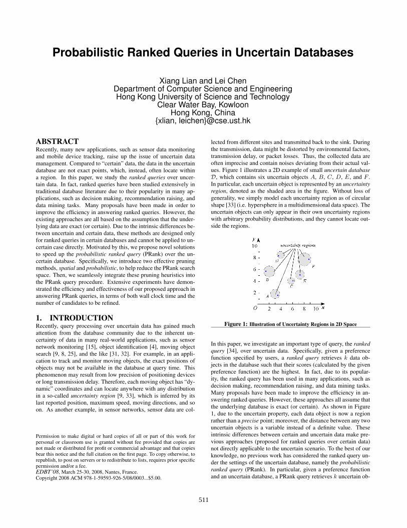
lected from different sites and transmitted back to the sink. Duringthe transmission, data might be distorted by environmental factors,transmission delay, or packet losses. Thus, the collected data areoften imprecise and contain noises deviating from their actual val-ues. Figure 1 illustrates a 2D example of small uncertain databaseD, which contains six uncertain objects A, B, C, D, E, and F .In particular, each uncertain object is represented by an uncertaintyregion, denoted as the shaded area in the figure. Without loss ofgenerality, we simply model each uncertainty region as of circularshape [33] (i.e. hypersphere in a multidimensional data space). Theuncertain objects can only appear in their own uncertainty regionswith arbitrary probability distributions, and they cannot locate out-side the regions.

Figure 1: Illustration of Uncertainty Regions in 2D Space

In this paper, we investigate an important type of query, the rankedquery [34], over uncertain data. Specifically, given a preferencefunction specified by users, a ranked query retrieves k data ob-jects in the database such that their scores (calculated by the givenpreference function) are the highest. In fact, due to its popular-ity, the ranked query has been used in many applications, such asdecision making, recommendation raising, and data mining tasks.Many proposals have been made to improve the efficiency in an-swering ranked queries. However, these approaches all assume thatthe underlying database is exact (or certain). As shown in Figure1, due to the uncertain property, each data object is now a regionrather than a precise point; moreover, the distance between any twouncertain objects is a variable instead of a definite value. Theseintrinsic differences between certain and uncertain data make pre-vious approaches (proposed for ranked queries over certain data)not directly applicable to the uncertain scenario. To the best of ourknowledge, no previous work has considered the ranked query un-der the settings of the uncertain database, namely the probabilisticranked query (PRank). In particular, given a preference functionand an uncertain database, a PRank query retrieves k uncertain ob-

511

jects that are expected to have the highest scores.

Figure 2 presents an example of ranked query in both traditional(containing “certain” objects) and uncertain databases. The pref-erence function f(

−→O ) is used to calculate the score of an object−→

O (O1, O2), where O1 and O2 are two coordinates of object−→O .

For the sake of simplicity, we use O to denote vector (object)−→O

throughout this paper. In the example, we assume the score, f(O),of object O is given by (O1 + O2), where the same weight (i.e. 1)is assigned to both dimensions. In a general case, different weightscan be introduced by users to bias the preference of different di-mensions. The line, f(O) = O1 +O2, in Figure 2 contains a set ofpoints that have the same score value (i.e. f(O)). In the traditionaldatabase of Figure 2(a), object E has the second largest score (onlysmaller than that of object F ). In an uncertain database, however,as illustrated in Figure 2(b), it is not clear any more whether ob-ject E indeed has the second largest score, since object D is alsoa potential candidate to have the second largest score. Therefore,we have to re-define the probabilistic ranked query in the contextof the uncertain database.

(a) Traditional Database (b) Uncertain Database

Figure 2: A 2D Example of Ranked Query

In this paper, we propose an efficient and effective approach toanswer the PRank query. Specifically, we provide effective prun-ing heuristics to significantly reduce the PRank search space, andutilize a multidimensional index to efficiently perform the PRankquery processing.

In particular, we make the following contributions.

1. We formalize a novel query, the probabilistic ranked query(PRank), in the context of uncertain databases.

2. We illustrate a general framework for answering the PRankquery, and propose effective pruning heuristics to help reducethe PRank search space.

3. We seamlessly integrate the proposed pruning methods intothe query procedure, which can efficiently retrieve the PRankquery results.

4. Last but not least, we demonstrate through extensive exper-iments the effectiveness of our pruning methods as well asthe efficiency of PRank query processing.

The rest of the paper is organized as follows. Section 2 brieflyoverviews previous methods to answer ranked queries over the tra-ditional “certain” database, as well as various query processingover uncertain databases. Section 3 formally defines our problem ofprobabilistic ranked query. Section 4 proposes the general frame-work and pruning heuristics for answering PRank queries. Sec-tion 5 presents the PRank query procedure to perform the PRank

search. Section 6 demonstrates the query performance of PRankunder different experimental settings. Finally, Section 7 concludesthis paper.

2. RELATED WORKSection 2.1 briefly reviews the ranked query in traditional databasesthat contain “certain” objects. Section 2.2 presents the query pro-cessing over uncertain databases.

2.1 Ranked Queries in Traditional DatabasesRanked query has many real applications such as decision mak-ing, recommendation raising, and data mining tasks. Specifically,given a d-dimensional database D and a linear preference functionf(·), a ranked query retrieves k objects O ∈ D, such that theircorresponding scores, f(O), are the highest in the database, wheref(O) =

∑di=1 wi · Oi (note: wi is a weight indicating the user’s

preference and Oi is the i-th coordinate of object O).

Due to the importance of ranked queries, many previous work fo-cus on efficient methods to retrieve the query answer. Specifically,Chang et al. [7] first proposed an Onion technique to perform theranked search. They consider each data object in the database D asa multidimensional point in the data space. Let CH1 be the (layer-1) convex hull of all the points in D, CH2 be the layer-2 convexhull of those points that are not in CH1 (i.e. D\CH1), and so on.In the general case, CHi is the layer-i convex hull of those pointsin D\(CH1 ∪ CH2 ∪ ... ∪ CHi−1). The basic idea of the Oniontechnique is as follows. The top-1 object (i.e. with rank 1) is al-ways in CH1; the second ranked object is always in CH1 ∪CH2;the third ranked one is in CH1∪CH2∪CH3; ...; and so on. There-fore, data objects can be pre-processed by sorting them accordingto their layer numbers. Whenever a ranked query that retrieves ktop-ranked objects arrives, the Onion algorithm starts scanning thedata set from the most-exterior (layer-1) convex hull (i.e. CH1) tolayer-k convex hull (i.e. CHk). All the retrieved objects are can-didate answers to the ranked query. A similar layer-based method,AppRI, has recently been proposed by Xin et al. [39].

Hristidis et al. [17, 18] provided a view-based approach, PRE-FER, to answer the ranked query. In particular, Hristidis et al. pre-defined some preference functions fv(·), and created a material-ized view for each function by sorting data objects in descendingorder of their scores. Given a query preference function f(·), PRE-FER first selects one of the pre-computed views, with respect to apreference function fv(·) that is the most similar to f(·), and thensequentially scans only a portion of this view, stopping at the wa-termark point. Another view-based technique, LPTA, proposed byDas et al. [13], also maintains sorted record id lists according tothe view’s preference functions.

Fagin et al. [14] proposed the threshold algorithm (TA) to answerthe top-k query, which is based on the ranked lists. Specifically,along each dimension i, they sort the data objects in descendingorder of the i-th coordinate. Thus, in a d-dimensional database,d sorted lists can be obtained, which are accessed sequentially in around-robin fashion. Whenever an object is obtained from a rankedlist, TA immediately computes its score. Let T be a score thresh-old defined as the maximum possible score for those objects thathave not been seen so far. If there exist k objects (that we haveseen so far) that have scores higher than T , then TA terminates andreports these k objects as the query result. In the context of rela-tional databases, many previous work also studied top-k queries,including [5, 6, 27, 37, 20, 23, 26].

512

Tao et al. [34] aimed to improve the retrieval efficiency of rankedqueries with the help of the R-tree index [16]. In particular, theyproposed a branch-and-bound ranked search (BRS) algorithm. BRSmaintains a maximum heap to help traverse the R-tree in a best-firstmanner, where the key of heap entry is defined as the maximumpossible score of data points in this entry. The query performanceof BRS is proved to be I/O optimal. Yiu et al. [42] defined top-k spatial preference queries, which also utilize the R-tree index toretrieve objects with high scores. Recently, there are some otherwork on the top-k query or its variants, to list a few of them, [40,24, 43, 1, 19, 3]. However, these work only handle certain data,and cannot be directly applied to uncertain databases, which mo-tivates us to propose a new method to answer ranked queries overuncertain data.

2.2 Query Processing in Uncertain DatabasesQuery processing over uncertain data has gained much attentiondue to its importance in many applications [15, 4, 9, 8, 25, 31, 32],where real-world data inherently contain uncertainty. For example,the Orion system [11] is a system for managing uncertain data inapplications such as sensor data monitoring. Previous studies haveconsidered many query types, such as range query [10, 12, 33],nearest neighbor query [9, 10, 22], skyline query [28], and sim-ilarity join [21], with which specific techniques are designed forsearching over uncertain databases. To the best of our knowledge,so far no existing work has studied the ranked query in the con-text of the uncertain database, which assumes that data objects canhave “dynamic” attributes in the data space (i.e. locating anywherewithin the uncertainty regions). Note that, although previous works[29, 32, 41] studied top-k queries in the probabilistic database, theyconsider the possible world semantics in relational databases [30,2], whereas our work focuses on the uncertain query processing inthe spatial database.

Due to the inherent uncertainty in many real-world data from vari-ous applications, previous methods to handle “certain” data cannotbe directly used and we have to find a solution which can efficientlyanswer the PRank query in uncertain databases, which is the focusof this paper.

3. PROBLEM DEFINITIONIn this section, we formally define the problem of the probabilisticranked query (PRank). In particular, assume we have a static uncer-tain database D in a d-dimensional space, in which each uncertainobject O(O1, O2, ..., Od) can locate anywhere within an (hyper-spherical) uncertainty region UR(O) [9, 33] centered at point CO

with radius rO . Let pdf(O) be the probability density function(pdf) with respect to the location that object O appears. We havepdf(O) ∈ [0, 1], if O ∈ UR(O); pdf(O) = 0, otherwise. Follow-ing the convention [10, 9, 28], we assume that all the data objectsare independent of each other in the database D. The problem ofretrieving the PRank query results is defined as follows.

DEFINITION 3.1. (Probabilistic k-Ranked Query, k-PRank) As-sume we have an uncertain databaseD, a user-specified preferencefunction f and an integer k. For 1 ≤ m ≤ k, we define the m-ranking probability Prm(O) of object O ∈ D as:

Prm(O) =

∫ s2

s1

Pr{f(O) = s} ·

∑

∀{P1,P2,...,Pm−1}∈D\{O}(1)

m−1∏

i=1

Pr{f(Pi) ≥ s} ·∏

∀Pj∈D\{O,P1,...,Pm−1}Pr{f(Pj) ≤ s}

ds.

Symbol DescriptionD the data set with data size |D|d the dimensionality of the data setUR(O) the uncertainty region of object Ok the number of uncertain objects to retrieve in the PRank queryf(O) the preference function with respect to object Ofv(O) the pre-defined preference functions to compute the lower/upper

bound probabilityl the weight resolutionn the number of pre-computed probabilistic bounds with respect to a

preference function fv(·) for each uncertain object

Table 1: Meanings of Symbols Used

where s1 and s2 are the lower and upper bounds of score f(O)for object O, respectively. A k-PRank query retrieves k uncertainobjects OR1, OR2, ..., ORm, ..., ORk (∈ D) such that objectORm has the highest m-ranking probability Prm(ORm) amongall data objects in D.

Intuitively, Eq. (1) defines the expected probability Prm(O) (i.e.m-ranking probability) that object O has the m-th largest scorein the database D. In particular, when the score f(O) of objectO is s ∈ [s1, s2], we consider all possible cases where there areexactly (m − 1) objects P1, P2, ..., and Pm−1 in D\{O} havinghigher scores than s (i.e. higher ranks than O), while the otherobjects Pj ∈ D\{O, P1, ..., Pm−1} have lower scores than objectO. Thus, as shown in Eq. (1), for each possible combination of P1,P2, ..., and Pm−1, we calculate the probability that O has the m-thhighest score by multiplying probabilities that objects have eitherhigher or lower scores than s (due to the object independence [10,9, 28]). Finally, we integrate the probability summation for all thesecombinations on s, and obtain the expected probability that O hasthe m-th rank. Note that, in a special case where k = 1, Eq. (1)can be rewritten as a much simpler form:

Prm(O) =

∫ s2

s1

Pr{f(O) = s} ·

∏

∀Pj∈D\{O}Pr{f(Pj) ≤ s}

ds. (2)

After defining the m-ranking probability, the problem of the PRankquery is to retrieve object OR1 that has the highest score with thehighest probability Pr1(OR1) among all the objects in D; objectOR2 that has the second highest score with the highest proba-bility Pr2(OR2); ...; and object ORk that has the k-th highestscore with the largest probability Prk(ORk). In this paper, weconsider linear preference function f(·) and leave other interest-ing preference functions as our future work. Specifically, we letf(O) =

∑di=1 wi · Oi, where wi are weights specified by the

PRank query.

Since previous approaches are designed only for the ranked queryprocessing over precise objects, they are not suitable for handlinguncertain data. Thus, the only straightforward method to answerPRank queries is probably the linear scan. That is, we sequentiallyscan all the uncertain objects on disk one by one and calculate theirexpected probabilities in Eq. (1) with which the PRank results aredetermined. However, since the probability integration in Eq. (1) isquite complex, this method incurs high cost in terms of both com-putations and page accesses (i.e. I/O cost). Motivated by this, inthe sequel, we aim to find pruning heuristics in order to effectivelyreduce the PRank search space and efficiently answer the query.Table 1 summarizes the commonly-used symbols in this paper.

513

4. PROBABILISTIC RANKED QUERIESAs mentioned earlier, the linear scan of the database incurs highcomputation and I/O costs. Thus, in order to speed up the proce-dure of answering probabilistic ranked queries (PRank), we indexthe uncertainty regions of data objects with a multidimensional in-dex. Note that, since our proposed methodology is independentof the underlying index, throughout this paper, we simply use oneof the popular indexes, R-tree [16]. In particular, R-tree recur-sively bounds the uncertainty regions of data objects with minimumbounding rectangles (MBRs), until one final node (i.e. the root) isobtained.

In the sequel, Section 4.1 presents a general framework for answer-ing the PRank query. Section 4.2 illustrates the heuristics of thespatial pruning method, where the location distributions of uncer-tain objects can be either known or unknown. With the knowledgeof the object distributions in their uncertainty region, Section 4.3further presents the idea of probabilistic pruning method. Section4.4 discusses the refinement of the PRank candidate set.

4.1 The General FrameworkFigure 3 illustrates a general framework for answering the PRankquery. In particular, the framework consists of four phases, in-dexing, pruning, bounding, and evaluation. In the first indexingphase, given an uncertain databaseD, we construct an R-tree indexI over D to facilitate the PRank query (line 1). As a second step,the pruning phase eliminates those uncertain objects that cannot bethe PRank result, using novel spatial and/or probabilistic pruningmethod(s) that we propose (line 2), in the case where the locationdistribution of each object is either known or unknown within itsuncertainty region. Next, in the retrieved candidate set, we con-ceptually bound those objects that are involved in the probabilitycalculation in Eq. (1) (called bounding phase) and finally refine thecandidates by computing the actual probability (in Eq. (1)) and re-turning answers in the evaluation phase (line 3). Below, we mainlyfocus on illustrating the pruning and bounding phases.

Procedure PRank_Framework {Input: a d-dimensional uncertain databaseD, a preference function f(·),

and an integer kOutput: k objects in the PRank query result(1) construct a multidimensional index structure I overD // indexing phase(2) perform spatial and/or probabilistic pruning over I // pruning phase(3) refine candidates and return the answer set

// bounding and evaluation phases}

Figure 3: The General Framework for PRank Queries

4.2 Spatial PruningIn this subsection, we first propose a novel spatial pruning methodto reduce the search space for k-PRank queries (k ∈ [1, +∞)).Specifically, our spatial pruning method aims at eliminating thosedata objects that are definitely not in the k-PRank result. In fact,the rationale behind spatial pruning is that if we can clearly knowthat there are more than k data objects whose scores are higher thanthat of an object O, then we can safely prune object O.

Figure 4(a) illustrates the previous example of small uncertain databaseD. In fact, since each uncertain object O can only locate within itsuncertainty region UR(O), the score f(O) of O can be boundedby an interval, say [LB_f(O), UB_f(O)]. For instance, object F(or D) has its score within [LB_f(F ), UB_f(F )] (or [LB_f(D),

(a) Lower and Upper Bounds of Scores (b) 2D Score-Object Space

Figure 4: Heuristics of Spatial Pruning Method

UB_f(D)]). Now we convert the score interval of each object intoa 2D score-object space, as shown in Figure 4(b), where the hor-izontal axis represents objects and the vertical one corresponds toscores. Assume we issue a 2-PRank query. From the figure, wefind that object D has the second largest lower bound LB_f(D)of score f(D). Moreover, objects A has its upper bound scoreUB_f(A) smaller than LB_f(D). In other words, there must ex-ist at least two data objects (e.g. D and F ) which have their scoresgreater than A. Thus, object A can be safely pruned. Similarly,the other two objects B and C can also be discarded. On the otherhand, for the last object E, however, since its upper bound score isgreater than LB_f(D), object E still has chance to be the queryresult, and thus it cannot be pruned.

We summarize our spatial pruning method as follows.

LEMMA 4.1. (Spatial Pruning) Given an uncertain databaseD, a user-specified preference function f(·) and an integer k, letP1, P2, ..., and Pk be the k uncertain objects that we have obtainedso far. Assume LB_f(Pk) is the smallest (i.e. k-th largest) lowerbound of score among these k objects. The spatial pruning methodcan safely filter object O (with score interval [LB_f(O), UB_f(O)])out, if UB_f(O) ≤ LB_f(Pk) holds.

Proof. According to the assumption of the lemma, there existat least k uncertain objects such that their scores are higher thanthat of object O. Thus, in Eq. (1), the probability integration (i.e.Prm(O)) of object O is always equal to zero. Hence, object O isguaranteed not to be in the k-PRank result, and thus can be safelypruned. 2

Computation of Lower and Upper Score Bounds. For spatialpruning, we need to get lower and upper score bounds for each un-certain object. We assume that the uncertainty region UR(O) of anuncertain object O is centered at point CO with radius rO . More-over, a query preference function is defined as f(O) =

∑di=1(wi ·

Oi) (wi > 0). Our goal is to find a data point X in UR(O), suchthat its score is either minimized or maximized. Formally, we wantto minimize/maximize f(X) =

∑di=1 wi ·Xi, under the constraint∑d

i=1(Xi−COi)2 ≤ r2

O . We solve this optimization problem andobtain the lower and upper bounds of score f(O), respectively.

LB_f(O) =

d∑

i=1

min

wi ·

COi ±

wi√∑dj=1 w2

j

· rO

, (3)

514

UB_f(O) =

d∑

i=1

max

wi ·

COi ±

wi√∑dj=1 w2

j

· rO

. (4)

4.3 Probabilistic PruningUp to now, we have discussed the spatial pruning method, wherethe location distributions of data objects can be either known or un-known in their uncertainty region. However, if we have such a dis-tribution knowledge (i.e. the location distributions of data objects),then we can further prune more uncertain objects by utilizing thisinformation. In this subsection, we propose a novel probabilisticpruning method to help answer the k-PRank query.

As indicated by Definition 3.1, any object O is in the answer setof a k-PRank query, if there exists an integer m ∈ [1, k] such thatobject O has the m-th largest score in the database with the high-est probability Prm(O) (defined in Eq. (1)). However, due to thecomplex probability integration in Eq. (1), it is quite inefficient tocalculate the actual probability Prm(O) directly. Thus, instead,the goal of our probabilistic pruning method is to find a probabil-ity interval [LB_Prm(O), UB_Prm(O)] that tightly bounds thecomplex Prm(O), and use this interval to efficiently prune dataobjects. The probabilistic pruning method can be summarized asfollows.

LEMMA 4.2. (Probabilistic Pruning) Given an uncertain data-base D, a user-specified preference function f(·) and an integer k,let P1, P2, ..., and Pk be the k uncertain objects that we haveobtained so far. Assume LB_Pr1, LB_Pr2, ..., and LB_Prk

are the lower bound probabilities of Pr1(P1), Pr2(P2), ..., andPrk(Pk), respectively, where Prm(Pm) is the maximum prob-ability in the database that an object Pm has the m-th largestscore. The probabilistic pruning method can safely prune those ob-jects O (with probability interval [LB_Prm(O), UB_Prm(O)]),if UB_Prm(O) ≤ LB_Prm(Pm) holds, for all m ∈ [1, k].

Proof. By contradiction. Assume object O should be included inthe PRank query result. Thus, based on Definition 3.1, O must havethe m-th largest score with the highest probability in the database,for some m ∈ [1, k]. However, according to the lemma assumptionthat UB_Prm(O) ≤ LB_Prm(Pm) for all m ∈ [1, k], object Oalways has the probability smaller than Pm for any m value, whichis contrary. Hence, our initial assumption is incorrect, and O canbe safely pruned. 2

Lemma 4.2 indicates that we can safely prune those objects thathave the m-th largest score in the database with low probability,for all m ∈ [1, k] among the data sets.

Next, we address the remaining issue, that is, how to obtain lowerand upper bound probabilities, LB_Prm(O) and UB_Prm(O),respectively, for probability Prm(O) calculated in Eq. (1). In par-ticular, within the integration of Eq. (1), we have to enumerate allpossible combinations of {P1, P2, ..., Pm−1}, which is very com-plex and costly. For simplicity, we denote S(N, m) as:

S(N, m) =∑

∀{P1,P2,...,Pm−1}∈D\{O}

(m−1∏

i=1

Pr{f(Pi) ≥ s}

·∏

∀Pj∈D\{O,P1,...,Pm−1}Pr{f(Pj) ≤ s}

(5)

where N is the data size of D\{O}.

Therefore, by substitute Eq. (5) into Eq. (1), now we can rewriteEq. (1) as:

Prm(O) =

∫ s2

s1

Pr{f(O) = s} · S(N, m)ds. (6)

Based on Eq. (6), in order to derive lower and upper bounds forPrm(O), it is sufficient to obtain lower and upper bounds of S(N,m), denoted as LB_S(N, m) and UB_S(N, m), respectively. Thereason is that:

Prm(O) ≥ LB_S(N, m) ·∫ s2

s1

Pr{f(O) = s}ds = LB_S(N, m), (7)

Prm(O) ≤ UB_S(N, m) ·∫ s2

s1

Pr{f(O) = s}ds = UB_S(N, m), (8)

which implies that LB_S(N, m) and UB_S(N, m) can be exactlyconsidered as lower and upper bounds of Prm(O), respectively.

Thus, below, we only need to calculate LB_S(N, m) and UB_S(N,m) for S(N, m), and simply let LB_Prm(O) = LB_S(N, m)and UB_Prm(O) = UB_S(N, m).

Note that, from Eq. (5), we can convert S(N, m) into its recursiveform. Specifically, we let G(Pi) = Pr{f(Pi) ≥ s}, and assumethe data set D\{O, P1, ..., Pm−1} contain objects Pm+1, Pm+2,..., and PN . We have the recursive function of S(N, m) as follows:

S(N, m) = S(N − 1, m) · (1−G(PN )) + S(N − 1, m− 1) ·G(PN ),S(N, 1) = (1−G(P1)) · (1−G(P2)) · ... · (1−G(PN )),S(m− 1, m) = G(P1) ·G(P2) · ... ·G(Pm−1).

(9)

Obviously, in Eq. (9), if we can find the lower and upper bounds ofG(Pi), denoted as LB_G(Pi) and UB_G(Pi), respectively, thenLB_S(N, m) and UB_S(N, m) can be easily computed. So, inthe sequel, we focus on the problem of bounding G(Pi), utilizingsome pre-computed probabilistic information.

We illustrate our intuition of finding LB_G(Pi) and UB_G(Pi)in an example of Figure 5. Assume we have an object Pi withits uncertainty region UR(Pi) as shown in the figure. Given aquery preference function f(Pi) =

∑dj=1 wj · Pij with G(Pi) =

Pr{f(Pi) ≥ s}, our problem is to compute lower and upper bounds,LB_G(Pi) and UB_G(Pi), of G(Pi), where s ∈ [s1, s2].

The intuition of our proposed method is somewhat similar to thatof PREFER [17]. However, compared to PREFER, which is de-signed for certain data, our proposal is more complex due to theuncertainty. In particular, we maintain a number of pre-definedpreference functions (e.g., fv(Pi) =

∑dj=1 vj · Pij in the exam-

ple). Similar to [17], preference functions, fv(O) =∑d

j=1 vj ·Oj ,are selected with a discretization of the weight domain (e.g. (0, 1])into l parts of equal size, where l is the weight resolution. For ex-ample, when l = 10, we have the pre-defined preference functionsfv(·), whose vj values come from 0.1, 0.2, ..., and 1.

For each fv(·), we further pre-compute n probabilistic bounds with

515

score thresholds tβ1 , tβ2 , ..., and tβn , with respect to every uncer-tain object Pi, such that object Pi has score greater than tβi withprobability equal to βi (i ∈ [1, n]), that is, Pr{fv(Pi) ≥ tβi} =βi ∈ [0, 1]. As illustrated in Figure 5, we have 5 bounds (i.e.n = 5) with tβ1 = t0.1, tβ2 = t0.3, tβ3 = t0.5, tβ4 = t0.7, andtβ5 = t0.9 (corresponding to 5 lines, respectively). For instance,the top line represents the function fv(Pi) = t0.1 (i.e. the score ofPi with fv(·) is equal to t0.1), where t0.1 is a score threshold suchthat Pr{fv(Pi) ≥ t0.1} = 0.1. The meanings of other bounds aresimilar.

Given a query preference function f(O) =∑d

j=1 wj · Oj , wewould choose one pre-computed preference function fv(·) whichis the most similar to f(·) [17]. Specifically, we pick up the pre-defined fv(·) with vj closest to wj in f(·) (e.g. if w1 = 0.23 andl = 10, then we select the one with v1 = 0.2).

By utilizing the pre-computed probabilistic bounds with respect tofv(·), we can obtain the upper bound UB_G(Pi) of G(Pi) as fol-lows. Since s ≥ s1, it holds that G(Pi) ≤ Pr{f(Pi) ≥ s1}.Moreover, as illustrated in Figure 5, since the line f(Pi) = s1 isabove line fv(Pi) = t0.7 within the uncertainty region UR(Pi),we have G(Pi) ≤ Pr{f(Pi) ≥ s1} ≤ Pr{fv(Pi) ≥ t0.7} =0.7. That is, we can set UB_G(Pi) to 0.7.

Similarly, for the lower bound LB_G(Pi) of G(Pi), due to s ≤ s2,it holds that G(Pi) ≤ Pr{f(Pi) ≥ s1}. Furthermore, Figure 5indicates that the line f(Pi) = s2 is below line fv(Pi) = t0.3

in UR(Pi). Therefore, we have G(Pi) ≥ Pr{f(Pi) ≥ s2} ≥Pr{fv(Pi) ≥ t0.3} = 0.3, resulting in LB_G(Pi) = 0.3.

Figure 5: Lower and Upper Bounds of G(Pi) for Object Pi

After introducing our intuition, now we formally give the boundsfor G(Pi). Specifically, given two preference functions fv(O) =∑d

j=1 vj · Oj and f(O) =∑d

j=1 wj · Oj , if f(Pi) = s, our goalis to find two tight (pre-computed) probabilistic bounds, fv(P−i )and fv(P+

i ), for fv(Pi), satisfying fv(P−i ) ≤ fv(Pi) ≤ fv(P+i ).

Note that, the two probabilities associated with these two boundsexactly correspond to the lower or upper bound of G(Pi). As in theprevious example of Figure 5, the bound with score threshold t0.7

is associated with the upper bound probability 0.7.

We have:

fv(Pi) = f(Pi)−d∑

j=1

(wj − vj) · Pij (10)

where Pi ∈ UR(Pi).

Without loss of generality, assume each coordinate Pij of Pi iswithin an interval [Lj , Hj ] inferred by the uncertainty region UR(Pi).Furthermore, we can obtain a even tighter bounding interval [L′j , H

′j ]

for Pij . In particular, since it holds that f(Pi) =∑d

j=1 wj ·Pij =s, we consider three cases for different values of wj as follows.

• Case 1 (wj = 0). L′j = Lj and H ′j = Hj .

•Case 2 (wj > 0). Since it holds that Pij =f(Pi)−

∑dl=1∧l 6=j wl·Pil

wj,

we havef(Pi)−

∑dl=1∧l6=j wl·Hl

wj≤ Pij ≤ f(Pi)−

∑dl=1∧l6=j wl·Ll

wj.

Thus, we have L′j = max{Lj ,f(Pi)−

∑dl=1∧l 6=j wl·Hl

wj} and H ′

j =

min{Hj ,f(Pi)−

∑dl=1∧l6=j wl·Ll

wj}.

• Case 3 (wj < 0). Similarly, we havef(Pi)−

∑dl=1∧l 6=j wl·Ll

wj≤

Pij ≤ f(Pi)−∑d

l=1∧l6=j wl·Hl

wj. Thus, we obtain L′j = max{Lj ,

f(Pi)−∑d

l=1∧l6=j wl·Ll

wj} and H ′

j = min{Hj ,f(Pi)−

∑dl=1∧l6=j wl·Hl

wj}.

By substituting either L′j or H ′j into Eq. (10), we can obtain the

lower and upper bounds (i.e. fv(P−i ) and fv(P+i ), respectively)

for fv(Pi). In particular, when wj ≥ vj , we let Pij = L′j in orderto obtain fv(P+

i ) and let Pij = H ′j to get fv(P−i ). In contrast,

when wj < vj , we set Pij = H ′j to obtain fv(P+

i ) and Pij = L′jto get fv(P−i ).

Therefore, after obtaining fv(P−i ) and fv(P+i ), we can find two

pre-computed probabilistic bounds, and in turn obtain the associ-ated probabilities (i.e. either LB_G(Pi) or UB_G(Pi)). WithLB_G(Pi) and UB_G(Pi), we can compute the bound of S(N, m)by recursive function in Eq. (9), which is exactly the bound forPrm(O). Note that, if we initially set m to k in Eq. (9), during thecalculation of lower/upper bound for S(N, k), we can obtain someside products from the intermediate results, that is, the lower/upperbound of S(N, m) for any m ∈ [1, k]. Therefore, some redundantcalculations with the same values of N and m can be significantlysaved.

Finally, we present an optimization method for computing the lower/ upper bound for S(N, m) (i.e. that for Prm(O)). Recall inEq. (9), that the recursion depth, N , is large, where N is the size ofD\{O}. However, one interesting observation is that, as long as itholds that UB_f(PN ) ≤ s1 = LB_f(O), we have G(PN ) = 0,and thus Eq. (9) can be simplified as S(N, m) = S(N − 1, m). Inother words, object PN would not affect the calculation of proba-bility S(N, m) if its score interval is entirely below that of objectO. In this way, we can efficiently calculate S(N, m) with only asmall subset of objects in the database.

In summary, in order to calculate the lower/upper bound of proba-bility Prm(O) in Eq. (1), we can offline select some preferencefunction fv(·), with each of which n probabilistic bounds withscore thresholds tβ1 , tβ2 , ..., and tβn are pre-computed for eachuncertain object O (like the one in Figure 5), where Pr{fv(O) ≥tβi} = βi. Then, upon the query’s arrival, we compute LB_G(Pi)and UB_G(Pi) using these bounds as discussed above, and even-tually obtain LB_S(N, m) and UB_S(N, m) (i.e. LB_Prm(O)and UB_Prm(O), respectively), which can be used in the proba-bilistic pruning method in Lemma 4.2.

516

4.4 Final RefinementIn previous subsections, we illustrate details of our pruning meth-ods, including both spatial and probabilistic pruning. After thepruning process, the remaining data objects that cannot be prunedare called the candidates of the k-PRank query. Since our pruningmethods can guarantee that all the discarded objects are not queryresults, the candidate set after pruning would contain all the queryanswers. However, false positives still exist in the candidate set (i.e.those objects that should not be query answers but are in the candi-date set). Therefore, we have to refine the candidate set in order toobtain the actual query results. In particular, we need to computethe actual probability (in Eq. (1) or equivalently Eq. (6)) that eachcandidate is in the PRank result and remove those false positives.

Similar to the optimization method (mentioned in the last paragraphof Section 4.3), from Eq. (9), for any s ∈ [s1, s2], as long as objectPN has its upper bound of score, UB_f(PN ), never greater thans1, object PN would not affect the calculation of S(N, m) at all(since S(N, m) = S(N − 1, m)). Thus, we only need to calculateS(N, m) (or Prm(O)) involving those objects that have their scoreupper bounds greater than s1 (which are the same objects as thoseduring probabilistic pruning to compute bounds).

Therefore, for the candidate set obtained after the spatial pruning,we can calculate the smallest score lower bound (e.g. s1) among allcandidates. Then, we further retrieve those objects that have theirscore upper bounds greater than s1, which are used first for prob-abilistic pruning and then the calculation of the actual probability(in Eq. (1) or Eq. (6)). This conceptual association of objects witheach candidate to compute the probability (or bounds) is called thebounding phase, as mentioned earlier in our PRank framework (inSection 4.1).

For those remaining candidates that cannot be pruned, our finalevaluation phase would calculate the actual probability in Eq. (1)(or Eq. (6)), applying the numerical method, similar to that used in[10, 9]. Since objects that are involved in the probability calcula-tion are bounded by our optimization method, the resulting compu-tation cost is expected to be much smaller, compared to the cost inthe entire database using the original definition.

5. QUERY PROCESSINGIn this section, we seamlessly integrate the pruning heuristics (i.e.spatial and probabilistic pruning) into our PRank query procedure.As mentioned earlier, since the only feasible method so far for an-swering PRank queries is the linear scan, which however incurshigh cost, we use an R-tree [16] to index all the uncertain ob-jects in the database and enhance the query efficiency. In partic-ular, for each uncertain object O, we insert its uncertainty regionUR(O) into the R-tree I, on which the PRank query is processed.Note that, in order to apply the probabilistic pruning method, weneed to choose a number of preference functions that cover thewhole space of possible queries, which has been addressed in PRE-FER [17]. Moreover, in the case of space limitations, the selec-tion of several best preference functions under the constraint canalso refer to [17], which is however not the focus of this paper.With every pre-defined preference function fv(·), we pre-computen probabilistic bounds for each uncertain object O, which can helpobtain the bounds LB_G(Pi) and UB_G(Pi), and thus in turnLB_S(N, m) and UB_S(N, m).

In the sequel, Section 5.1 first illustrates how to prune intermediateentries in the R-tree index with the spatial pruning. Then, Section

5.2 presents the details of our PRank query procedure over the R-tree.

5.1 Pruning Intermediate EntriesIn this subsection, we discuss the heuristics of pruning intermediateentries in the R-tree. Obviously, an intermediate entry of R-tree canbe safely pruned if and only if all the uncertain objects under thisentry can be discarded. In the context of our k-PRank query, wecan safely prune an intermediate entry if the maximum score inthis entry is still smaller than that of at least k uncertain objects.In particular, we summarize the rationale of pruning intermediateentries in the following lemma.

LEMMA 5.1. (Spatial Pruning of Intermediate Entries) Assumewe have an R-tree index I constructed over uncertain database D,a user-specified preference function f(·) and an integer k. Let P1,P2, ..., and Pk be any k uncertain objects that we have obtained sofar, and e be an intermediate entry in I with the maximum possiblescore UB_f(e) (i.e. max{f(x)|∀x ∈ e}). Without loss of gen-erality, assume LB_f(Pk) is the smallest (i.e. k-th largest) lowerbound of score among these k objects. Thus, entry e can be safelypruned if it holds that UB_f(e) ≤ LB_f(Pk).

Proof. Similar to Lemma 4.1, since the largest possible score,UB_f(e), for any point in intermediate entry e is never greaterthan LB_f(Pk), it indicates that at least k objects P1, P2, ..., andPk have scores higher than any object in e. Thus, it is guaranteedthat entry e can be safely pruned. 2

According to Lemma 5.1, given an intermediate entry e, we onlyneed to calculate the maximum possible scores UB_f(e) in thisentry with respect to the preference function f(·), and compareit with LB_f(Pk). Note that, in the lemma, P1, P2, ..., and Pk

can be arbitrary k uncertain objects that we have accessed so far.Obviously, from the pruning condition UB_f(e) ≤ LB_f(Pk),the larger LB_f(Pk) is, the higher the pruning ability is. Thus, wecan set LB_f(Pk) to the k-th largest lower bound of scores, for allthe uncertain objects that we have obtained so far.

Furthermore, in order to compute the maximum score of an entry e,with respect to preference function f(·), we can use a hypersphereto bound the MBR of e, and then calculate the maximum possiblescore within the hypersphere. Specifically, let Ce be the centerpoint of e, and re be the radius of the hypersphere. Similar to thecomputation of the score upper bound for an uncertainty regionUR(O), it is sufficient to replace COi and rO in Eq. (4) with Ce

and re, respectively, in order to obtain UB_f(e).

5.2 Query ProcedureAfter discussing the heuristics of pruning intermediate entries (spa-tial pruning) in the R-tree, in this subsection, we continue to illus-trate the PRank query processing over the R-tree index in details.

In particular, Figure 6 presents the detailed query procedure, namelyPRank_Processing, for PRank. Procedure PRank_Processingtakes three parameters as input (i.e. an R-tree index I over uncer-tain database D, a query preference function f(·), and an integerk), and outputs k uncertain objects that are in the k-PRank queryresult.

In order to facilitate the PRank query processing, we maintain amaximum heap H accepting entries in the form (e, key), where e

517

Procedure PRank_Processing {Input: R-tree I constructed overD, preference function f(·), integer kOutput: k objects in the PRank query result(1) initialize a max-heapH accepting entries in the form (e, key)(2) Scand = Φ, Srfn = Φ, kLB_score = −∞;(3) insert (root(I), 0) into heapH(4) whileH is not empty(5) (e, key) = de-heapH(6) if key ≤ kLB_score, then break; // Lemma 5.1(7) if e is a leaf node(8) for each uncertain object O in e (sorted in descending order of LB_f(O))(9) if |Scand| < k(10) Scand = Scand ∪ {O}(11) if LB_f(O) > kLB_score(12) kLB_score = LB_f(O)(13) else // |Scand| ≥ k(14) if UB_f(O) ≥ kLB_score // spatial pruning, Lemma 4.1(15) if LB_f(O) > kLB_score(16) kLB_score = LB_f(O) // update kLB_score(17) let O′ be uncertain object(s) in Scand

satisfying UB_f(O′) < kLB_score(18) move object(s) O′ from Scand to Srfn

(19) Scand = Scand ∪ {O}(20) else // intermediate node(21) for each entry ei in e(22) if UB_f(ei) > kLB_score // Lemma 5.1(23) insert (ei, UB_f(ei)) into heapH(24) else(25) Srfn = Srfn ∪ {ei}(26) rlt = Probabilistic_Pruning (Scand, Srfn, f(·), k);(27) rlt = Evaluation (rlt, Scand, Srfn, f(·), k);(28) return rlt

}

Figure 6: PRank Query Processing

is either a data object or an MBR node, and key is defined as themaximum score UB_f(e) of any point in e, with respect to pref-erence function f(·) (line 1). Moreover, we also keep a candidateset Scand containing candidates of the k-PRank query, and a re-finement set, Srfn, of objects/MBRs that are involved in the prob-abilistic pruning and/or the final evaluation phase. Furthermore, aparameter kLB_score is initialized by negative infinity, represent-ing the k-th largest score lower bound, for all the objects that havebeen seen so far (line 2).

Our query procedure PRank_Processing traverses the R-tree in-dex by accessing heap entries in descending order of their keys.Specifically, we first insert the root root(I) of R-tree I into heapH (line 3). Every time we pop out an entry (e, key) from heap Hwith the largest key (lines 4-5). Recall that, the key, key, is de-fined as the maximum possible score of an object or any point inan MBR node. Thus, if it holds that largest key, key, in heap His never greater than kLB_score (i.e. the k-th largest score lowerbound that we have seen so far), then all the remaining entries inheap H can be safely pruned and the traversal of R-tree can be ter-minated (line 6); otherwise, we need to check entry e as shownbelow.

When the entry e we obtain from heap H is a leaf node, we ver-ify uncertain objects O in e in the descending order of f(O) (forthe sake of achieving higher pruning power, lines 7-8). In thecase where the number of candidates in Scand is less than k, wesimply add object O to Scand and moreover update the variablekLB_score (lines 9-12). Furthermore, if the size of candidate setis greater than or equal to k, then we perform the spatial prun-ing as given in Lemma 4.1 (line 14). That is, if the upper boundof score for object O is smaller than kLB_score, then there ex-ist at least k objects in Scand such that their scores are higherthan f(O), and object O can thus be safely pruned; otherwise(i.e. UB_f(O) ≥ kLB_score), we have to update the variable

kLB_score (lines 14-18) as well as the candidate set Scand (line19). In particular, if it holds that LB_f(O) > kLB_score, thenwe can obtain an even higher kLB_score, and meanwhile removethose object(s) O′ ∈ Scand such that UB_f(O′) is smaller thanthe newly updated kLB_score (lines 15-18). Note that, althoughO′ is guaranteed not to be the PRank result by our pruning method,it may still be needed for calculating the probability in Eq. (1) dur-ing the probabilistic pruning or evaluation phase. Therefore, we donot discard object(s) O′, but insert it (them) into the refinement setSrfn (line 18).

When the entry e is an intermediate node in the R-tree, we checkthe pruning condition for each entry ei in e, applying Lemma 5.1(lines 20-22). Specifically, for each entry ei in e, in case the max-imum possible score UB_f(ei) in ei is greater than kLB_score,we have to insert ei into heap H, in the form (ei, UB_f(ei)), forlater access (since there may exist PRank answers in ei, lines 22-23); otherwise, we can safely prune entry ei. However, similar tothe case of data object O′ (line 17), we add ei to the refinementset Srfn (lines 24-25), since objects in ei may affect the calcula-tion of probability for candidates during the probabilistic pruningor evaluation phase.

Next, we discuss the procedure Probabilistic_Pruning invoked byline 26 in procedure PRank_Processing. After the spatial prun-ing, we obtain a set, Scand, of PRank candidates. Moreover, the re-finement set Srfn contains objects/MBRs that may help prune/refinethese candidates (note that Srfn does not contain any PRank candi-dates). Since the probability integration in Eq. (1) is very complexand costly, we perform the probabilistic pruning to further reducethe candidate size.

The basic rationale of procedure Probabilistic_Pruning is as fol-lows. First, we retrieve those data objects in Srfn that may affectthe calculation of the lower/upper bound probability for PRank can-didates in Scand (according to the optimization method mentionedin Section 4.3). As a second step, we compute the lower/upperbound of probability for each candidate and apply the probabilisticpruning in Lemma 4.2.

In particular, Figure 7 shows the details of our pruning procedureover the candidate set Scand. The procedure Probabilistic_Pruningfirst finds the smallest score lower bound, min_score, within thecandidate set Scand (line 1). Then, we search over the two setsScand and Srfn, and retrieve all the data objects O′ such thatUR_f(O′) ≥ min_score (for any intermediate node e in Srfn,its subtrees are traversed in a best-first manner), which are insertedinto an initially empty set R (lines 3-7). As mentioned in thelast paragraph of Section 4.3 (i.e. the optimization method), onlythose objects in R are necessary to be checked for the probabil-ity calculation of each candidate. After that, for each candidateO ∈ Scand, we compute the lower and upper bounds of Prm(O)(for all m ∈ [1, k]) only involving objects in R (lines 8-9). Fi-nally, we apply the probabilistic pruning method in Lemma 4.2to prune candidates in Scand, utilizing the computed lower/upperbound (line 10). The remaining candidates that cannot be prunedare returned as output (line 11).

In line 27 of procedure PRank_Processing, after the probabilisticpruning, we further refine the returned candidates (in the set rlt)in procedure Evaluation. Specifically, for each m ∈ [1, k], wecompute the actual probability of each candidate that has the m-th largest score (Eq. (1) or equivalently Eq. (6)), and select the one

518

Procedure Probabilistic_Pruning {Input: candidate set Scand, refinement set Srfn, preference function f(·),

integer kOutput: candidate set rlt for the PRank query(1) let min_score be the minimum score lower bound LB_f(O) for all the

candidates O in Scand

(2) R = Φ;(3) for each object/entry e in Scand ∪ Srfn

(4) if e is object and UB_f(e) ≥ min_score(5) R = R ∪ {e}(6) else // e is a node(7) add all the objects O′ under e to R satisfying UB_f(O′) ≥ min_score(8) for each candidate O ∈ Scand

(9) calculate the upper and lower bounds of Prm(O) over R// Section 4.3

(10) use the lower/upper bound of Prm(O) to prune candidates in Scand

// Lemma 4.2(11) return the remaining candidates

}

Figure 7: Procedure for Probabilistic Pruning

with the highest probability as the final result (i.e. PRankm). Notethat, similar to the probabilistic pruning, the calculation of Eq. (1)or Eq. (6) only needs to involve those objects in R, as computed inprocedure Probabilistic_Pruning, compared to that over the entiredatabase in the original definition.

In summary, since our query procedure PRank_Processing tra-verses the R-tree index in a best-first manner, in which each in-termediate node is accessed at most once, our query processing isefficient. Moreover, since we apply both spatial and probabilis-tic pruning methods, the resulting number of candidates should besmall, which will be confirmed later in our experiments.

6. EXPERIMENTAL EVALUATIONIn this section, we empirically evaluate the query performance ofour proposed approach to answer the probabilistic ranked query(PRank). In particular, since there are no real data sets available,we synthetically generate uncertain objects in a d-dimensional dataspace U = [0, 1]d, like the ones in [9, 12, 33]. Specifically, foreach uncertain object O, we first decide the center location CO

of its uncertainty region UR(O), and then randomly produce theradius rO of UR(O) within [rmin, rmax]. In order to simulatethe distribution of object position, for each uncertain object O, wegenerate 100 samples contained in its uncertainty region UR(O),following either Uniform or Gaussian distribution (with mean COi

and variance 2rO/5 along the i-th dimension). For brevity, we de-note lU (lS) as the data set with center locations CO of Uniform(Skew with skewness 0.8) distribution, rU (rG) as that with radiusrO ∈ [rmin, rmax] of Uniform (Gaussian, with mean (rmin +rmax)/2 and variance (rmax−rmin)/5) distribution, and pU (pG)as that with object position (in the uncertainty region) of Uniform(Gaussian) distribution. Thus, with different combinations, wecan obtain eight types of synthetic data sets, lUrUpU , lUrUpG,lUrGpU , lUrGpG; lSrUpU , lSrUpG, lSrGpU , and lSrGpG.Note that, for data sets with other distribution parameters (e.g. meanand variance for Gaussian, or skewness for Skew), the experimentalresults are similar, and we would not present all of them here. Af-ter generating data sets, we index them with R-tree [16], on whichPRank queries can be processed, where the page size is set to 1KB.

In order to evaluate the PRank query, we randomly generate 100query preference functions, f(O) =

∑di=1 wi ·Oi, as follows. For

each weight wi (1 ≤ i ≤ d), we randomly pick up a value withindomain (0, 1], following specific (Uniform, Gaussian, or Skew) dis-tribution (note that the results with negative weights are similarand thus omitted due to space limit). To enable the probabilis-

Parameter Values[rmin, rmax] [0, 0.01], [0, 0.02], [0, 0.03], [0, 0.04], [0, 0.05]k 2, 4, 6, 8, 10, 20d 2, 3, 4, 5N 10K, 20K, 30K, 40K, 50K, 100Kl 5, 8, 10, 20, 40n 5, 8, 10, 15, 20weight distribution Uniform, Gaussian, Skew

Table 2: The Parameter Settings

tic pruning method, we pre-select preference functions, fv(O) =∑di=1 vi · Oi (w ∈ (0, 1]), with the weight resolution l [17]. Fur-

thermore, with respect to any pre-defined preference function fv(·),for each uncertain object O, we pre-compute n probabilistic boundsas discussed in Section 4.3. That is, we obtain n score thresholdstβ1 , tβ2 , ..., tβn , such that Pr{fv(O) ≥ tβi} = βi, for 1 ≤ i ≤ n.For the sake of simplicity, here we let βi = i/n.

Throughout our experiments, we measure the wall clock time andthe number of PRank candidates to be refined (in the evaluationphase), in order to study the efficiency and effectiveness of ourPRank query procedure as well as the pruning methods. In partic-ular, the wall clock time is the time cost of retrieving PRank can-didates before the final evaluation phase, where we incorporate thecost of each page access (i.e. one I/O) by penalizing 10ms [35, 36].Thus, the wall clock time includes both the CPU time and I/O cost.Moreover, the number of PRank candidates to be refined is calcu-lated by summing up the number of candidates with rank m, for allm ∈ [1, k] (i.e., each object might be counted multiple times).

To the best of our knowledge, no previous work on PRank problemhas been studied in the context of uncertain databases. Therefore,the most naïve method is the linear scan, which sequentially scansthe entire uncertain database object by object on disk and finds outthe answer to the PRank query. To give an example, assume anuncertain database contains 30K 3D data objects. If the page sizeis 1KB and a floating number takes up 4 bytes, the I/O cost ofeven one linear scan requires about 3.6 (= 10ms

1000ms/s× 30K×3×4

1K)

seconds which is much greater than that of our method as shownbelow. In the sequel, we also illustrate the speed-up ratio of ourapproach compared with the linear scan, which is defined as therequired wall clock time of the linear scan (underestimated by onlyconsidering the I/O cost) divided by that of our method. As we willsee, our method can outperform the linear scan in terms of the wallclock time by orders of magnitude.

In each of the subsequent experiments, we vary the value of one pa-rameter while fixing others to their default values. Table 2 summa-rizes the parameter settings, where the default values of parametersare in bold font. All our experiments are conducted on a PentiumIV 3.2GHz PC with 1G memory, and the reported results are theaverage of 100 queries.

6.1 Performance vs. Radius Range [rmin, rmax]In the first set of experiments, we evaluate the efficiency and effec-tiveness of our proposed PRank query procedure using data setsthat have different radius ranges [rmin, rmax] for uncertain ob-jects. In particular, we test the wall clock time and the number ofPRank candidates to be refined over eight types of data sets, withranges [rmin, rmax] set to [0, 0.01], [0, 0.02], [0, 0.03], [0, 0.04],and [0, 0.05], where other parameters are set to their default valuesin Table 2 (i.e. the data size N is 30K, the dimensionality d is 3, thenumber, k, of query results (for k-PRank queries) is 6, the weight

519

(a) lU (b) lS

Figure 8: Performance vs. Radius Range [rmin, rmax]

resolution, l, is 10 and the number of probabilistic bounds, n, is setto 10). Furthermore, the query preference function is generated byselecting a random value wi ∈ (0, 1] as weight following Uniformdistribution. We will show later the effect of parameters l and n onthe query performance, as well as other weight distributions (e.g.Gaussian and Skew).

Figure 8 illustrates the experimental results by varying the radiusrange of 8 data sets. Figure 8(a) shows the results of 4 lU data setsand Figure 8(b) presents that of the remaining 4 lS ones. Note that,in all figures of experimental results, the numbers without bracketsover columns indicate the numbers of PRank candidates to be re-fined (i.e. calculating the actual probability integration in Eq. (1))in the evaluation phase, whereas those in brackets over columns arethe speed-up ratio of our methods, compared with the linear scan(i.e. underestimated by only considering the I/O cost).

From figures, we find that, when the radius range [rmin, rmax]varies from [0, 0.01] to [0, 0.05], the wall clock time of retrievingthe PRank candidates increases. This is reasonable, since largeruncertainty regions of data objects would make the ranks of un-certain objects much more indistinguishable. Thus, more PRankcandidates will be included in the candidate set, as confirmed bynumbers in figures, which makes the pruning process more costly.In general, however, the wall clock time of our PRank procedureis very efficient (less than 0.44 second for lU data sets and 0.12second for lS data sets). Observe that, lS data sets require muchless processing time than lU . This is because most data in lS datasets tend to have small values along each dimension (i.e. locatingtowards the origin), and only a few (sparse) data locate in spaceswith high scores, which thus has much less PRank candidates tocheck the pruning conditions, compared with lU data sets. It isinteresting to see the same phenomena in all the subsequent exper-iments. Furthermore, for all the data sets, the number of PRankcandidates to be refined remains small, compared with the totaldata size 30K; moreover, the speed-up ratio is significant, indi-cating that our method can outperform the linear scan by orders ofmagnitude.

6.2 Performance vs. kAs a second step, we evaluate the query performance of our pro-posed approach, with respect to different k values specified byPRank queries. In particular, Figure 9 illustrates the wall clock timeof PRank query procedure, over eight types of data sets, by vary-ing k from 2 to 20, where other parameters are set to their defaultvalues.

From the experimental results, the pruning efficiency of our pro-posed method is not very sensitive to the k value, in terms of thewall clock time. As we can see, the required wall clock time is

(a) lU (b) lS

Figure 9: Performance vs. k

(a) lU (b) lS

Figure 10: Performance vs. Dimensionality d

merely less than 0.18 (0.11) second for lU (lS) data sets in Figure9(a) (Figure 9(b)). When k grows larger, the number of resultingPRank candidates to be refined increases (since we maintain can-didates with rank m for each m from 1 to k). Moreover, from thespeed-up ratio in figures, we find that our approach can performorders of magnitude better than the linear scan.

6.3 Performance vs. Dimensionality dNext, we study the effect of dimensionality d for data sets on thePRank query performance. Specifically, we present the experimen-tal results over eight data sets in Figure 10, where other parametersare set to their default values.

Note that, since the data size N in our experiments is fixed to 30K,data in 2D space will be much more dense than that in higher di-mensional (e.g. 5D) space. Thus, the number of resulting PRankcandidates would decrease with the increasing dimensionality, asconfirmed by the results in figures. Moreover, when d = 2, data setlUrGpG (in Figure 10(a)) incurs higher wall clock time than thatof 3D case, due to the high cost of retrieving more candidates in the2D space.

For the reason of the dimensionality problem with multidimen-sional index (e.g. the query efficiency of R-tree [16] degrades withthe increasing dimensionality [38]), the wall clock time over eightdata sets basically increases when the dimensionality varies from 2to 5. However, the required time is still very low, that is, at most 0.7and 0.3 seconds for lU and lS data sets, respectively. Comparedwith the linear scan, the speed-up ratio is by order(s) of magnitude.

6.4 Performance vs. Data Size NIn this subsection, we test the scalability of our proposed PRankquery procedure, as a function of the data size, N . Specifically,we vary the data size N from 10K to 100K, and test the queryperformance over eight data sets, where other parameters are setto their default values. From figures, we find that the wall clocktime increases when the data size N becomes large. The reason

520

(a) lU (b) lS

Figure 11: Performance vs. Data Size N

(a) lU (b) lS

Figure 12: Performance vs. Weight Resolution l

is that, large data size results in high density of data objects in thespace, which incurs high cost to filter out unqualified objects. Thetotal required wall clock time, however, is less than 0.3 and 0.15for lU and lS data sets, as illustrated in Figures 11(a) and 11(b),respectively.

In general, the number of PRank candidates increases smoothlywith respect to the increasing data size; moreover, the speed-upratio of our method compared with the linear scan also increaseswhen N grows. These facts indicate the good scalability of ourproposed method in answering PRank queries, with respect to thedata size N .

6.5 Performance vs. Weight Resolution lIn this subsection, we study the effect of weight resolution l on thePRank query performance. Recall that, we divide the weight do-main (0, 1] into l intervals of equal size, and preference functionsfv(·) are pre-selected accordingly [17]. Then, given a query prefer-ence function f(·), we always choose one pre-computed preferencefunction fv(·) with weights the most similar to that of f(·). Intu-itively, the larger l is, the more similar the chosen fv(·) is to f(·).

Figure 12 illustrates the experimental results by varying the weightresolution l from 5 to 40 over 8 data sets, where other parametersare set to their default values. As expected, for some data sets, thenumber of PRank candidates to be refined decreases when l grows.However, the increasing trend is not very fast with respect to l,which indicates that our query procedure is not sensitive to l verymuch.

With the increasing l values, the wall clock time of all the 8 datasets remains approximately the same, which is only less than 0.18(0.11) second for lU (lS) data sets in Figure 12(a) (Figure 12(b)).Similarly, the speed-up ratio is nearly constant with respect to l,which shows the good performance of our method compared withthe linear scan.

(a) lU (b) lS

Figure 13: Performance vs. The Number of Probabilistic Bounds n

(a) lU (b) lS

Figure 14: Performance vs. Weight Distribution

6.6 Performance vs. Number of ProbabilisticBounds n

In this set of experiments, we test the PRank query performance ofour approach over 8 data sets in Figure 13, by varying the numberof probabilistic bounds, n, from 5 to 20, where other parametersare set to their default values.

Recall that, in order to perform the probabilistic pruning method,we need to pre-compute n probabilistic bounds so that the lower /up-per bounds of probabilities can be calculated. Intuitively, a largernumber of pre-computed bounds would give tighter bounds andhigher pruning ability. From figures, we can see that, when n in-creases, some data sets indeed show slightly fewer PRank candi-dates, which result in lower refinement cost (for other data sets,the decrease is not that significant). Moreover, the wall clock timeand speed-up ratio are not very sensitive to the n values. Note that,since a large n would also lead to large space to store pre-computedinformation, the experimental results shown in Figure 13 indicatethat we can choose a small n value (e.g. 10) to make a trade-offbetween space and query efficiency.

6.7 Performance vs. Weight DistributionFinally, we present the query performance of our proposed ap-proach with different weight distributions. Apart from the Uniformweight distribution that we used in previous experiments, we alsocompare it with Gaussian and Skew weight distributions. In par-ticular, Figure 14 illustrates the wall clock time of PRank queryprocessing over 8 types of data sets, using Uniform, Gaussian, andSkew weight distributions, where other parameters are set to theirdefault values.

From figures, we can see that our method is efficient with differentweight distributions, that is, less than 0.5 and 0.2 seconds are re-quired for lU and lS data sets, as shown in Figures 14(a) and 14(b),respectively. The results with Skew distribution require more wallclock time (thus lower speed-up ratio), since more PRank candi-dates are retrieved from the index.

521

7. CONCLUSIONSDue to the inherent uncertainty of data in many real-world applica-tions, query processing over these uncertain data becomes more andmore important. In the traditional “certain” database, the rankedquery has many applications like decision making, recommenda-tion raising, and data mining tasks. Previous query processingmethods, however, are inapplicable to the handle uncertain data.Motivated by this, in this paper, we propose a formal definition ofthe ranked query over uncertain databases, namely the probabilisticranked query (PRank), and design two effective pruning methods,spatial and probabilistic, to facilitate reducing the PRank searchspace. Moreover, we seamlessly integrate these two pruning heuris-tics into our PRank query procedure. Extensive experiments haveverified the efficiency and effectiveness of our proposed approach,in terms of the wall clock time and the number of PRank candidatesto be refined. Since our work assumes linear preference functions,in future, it would be interesting to consider arbitrary monotonicfunctions. Furthermore, another interesting direction is to studydiscrete PRank queries with uncertain categorical data.

8. ACKNOWLEDGMENTFunding for this work was provided by Hong Kong RGC Grant No.611907, National Grand Fundamental Research 973 Program ofChina under Grant No. 2006CB303000, and the NSFC Key ProjectGrant No. 60533110.

9. REFERENCES[1] R. Akbarinia, E. Pacitti, and P. Valduriez. Best position algorithms

for top-k queries. In VLDB, pages 495–506, 2007.[2] L. Antova, C. Koch, and D. Olteanu. Query language support for

incomplete information in the MayBMS system. In VLDB, pages1422–1425, 2007.

[3] B. Arai, G. Das, D. Gunopulos, and N. Koudas. Anytime measuresfor top-k algorithms. In VLDB, pages 914–925, 2007.

[4] C. Böhm, A. Pryakhin, and M. Schubert. The Gauss-tree: efficientobject identification in databases of probabilistic feature vectors. InICDE, page 9, 2006.

[5] N. Bruno, S. Chaudhuri, and L. Gravano. Top-k selection queriesover relational databases: Mapping strategies and performanceevaluation. TODS, 2002.

[6] K. C.-C. Chang and S.-W. Hwang. Minimal probing: supportingexpensive predicates for top-k queries. In SIGMOD, pages 346–357,2002.

[7] Y.-C. Chang, L. D. Bergman, V. Castelli, C.-S. Li, M.-L. Lo, andJ. R. Smith. The Onion technique: indexing for linear optimizationqueries. In SIGMOD, pages 391–402, 2000.

[8] L. Chen, M. T. Özsu, and V. Oria. Robust and fast similarity searchfor moving object trajectories. In SIGMOD, pages 491–502, 2005.

[9] R. Cheng, D. Kalashnikov, and S. Prabhakar. Querying imprecisedata in moving object environments. In TKDE, volume 16, pages1112–1127, 2004.

[10] R. Cheng, D. V. Kalashnikov, and S. Prabhakar. Evaluatingprobabilistic queries over imprecise data. In SIGMOD, pages551–562, 2003.

[11] R. Cheng, S. Singh, and S. Prabhakar. U-DBMS: A database systemfor managing constantly-evolving data. In VLDB, pages 1271–1274,2005.

[12] R. Cheng, Y. Xia, S. Prabhakar, R. Shah, and J. Vitter. Efficientindexing methods for probabilistic threshold queries over uncertaindata. In VLDB, pages 876–887, 2004.

[13] G. Das, D. Gunopulos, N. Koudas, and D. Tsirogiannis. Answeringtop-k queries using views. In VLDB, 2006.

[14] R. Fagin, A. Lotem, and M. Naor. Optimal aggregation algorithmsfor middleware. In PODS, pages 102–113, 2001.

[15] A. Faradjian, J. Gehrke, and P. Bonnet. Gadt: A probability space

ADT for representing and querying the physical world. In ICDE,pages 201–211, 2002.

[16] A. Guttman. R-trees: a dynamic index structure for spatial searching.In SIGMOD, pages 47–57, 1984.

[17] V. Hristidis, N. Koudas, and Y. Papakonstantinou. PREFER: Asystem for the efficient execution of multi-parametric ranked queries.In SIGMOD, 2001.

[18] V. Hristidis and Y. Papakonstantinou. Algorithms and applicationsfor answering ranked queries using ranked views. VLDBJ,13(1):49–70, 2004.

[19] M. Hua, J. Pei, A. W.-C. Fu, X. Lin, and H.-F. Leung. Efficientlyanswering top-k typicality queries on large databases. In VLDB,pages 890–901, 2007.

[20] I. F. Ilyas, W. G. Aref, and A. K. Elmagarmid. Supporting top-k joinqueries in relational databases. VLDBJ, 13(3):207–221, 2004.

[21] H.-P. Kriegel, P. Kunath, M. Pfeifle, and M. Renz. Probabilisticsimilarity join on uncertain data. In DASFAA, 2006.

[22] H.-P. Kriegel, P. Kunath, and M. Renz. Probabilistic nearest-neighborquery on uncertain objects. In DASFAA, 2007.

[23] C. Li, K. C.-C. Chang, I. F. Ilyas, and S. Song. RankSQL: Queryalgebra and optimization for relational top-k queries. In SIGMOD,pages 131–142, 2005.

[24] C. Li, M. Wang, L. Lim, H. Wang, and K. C.-C. Chang. Supportingranking and clustering as generalized order-by and group-by. InSIGMOD, pages 127–138, 2007.

[25] V. Ljosa and A. K. Singh. APLA: indexing arbitrary probabilitydistributions. In ICDE, pages 247–258, 2007.

[26] Y. Luo, X. Lin, W. Wang, and X. Zhou. Spark: Top-k keyword queryin relational databases. In SIGMOD, pages 115–126, 2007.

[27] A. Marian, N. Bruno, and L. Gravano. Evaluating top-k queries overweb-accessible databases. TODS, 29(2):319–362, 2004.

[28] J. Pei, B. Jiang, X. Lin, and Y. Yuan. Probabilistic skylines onuncertain data. In VLDB, 2007.

[29] C. Re, N. Dalvi, and D. Suciu. Efficient top-k query evaluation onprobabilistic data. In ICDE, 2007.

[30] R. Ross, V. S. Subrahmanian, and J. Grant. Aggregate operators inprobabilistic databases. J. ACM, 52(1):54–101, 2005.

[31] A. D. Sarma, O. B., A. Y. Halevy, and J. Widom. Working models foruncertain data. In ICDE, page 7, 2006.

[32] M. A. Soliman, I. F. Ilyas, and K. C. Chang. Top-k query processingin uncertain databases. In ICDE, 2007.

[33] Y. Tao, R. Cheng, X. Xiao, W. K. Ngai, B. K., and S. Prabhakar.Indexing multi-dimensional uncertain data with arbitrary probabilitydensity functions. In VLDB, pages 922–933, 2005.

[34] Y. Tao, V. Hristidis, D. Papadias, and Y. Papakonstantinou.Branch-and-bound processing of ranked queries. Inf. Syst.,32(3):424–445, 2007.

[35] Y. Tao, D. Papadias, and X. Lian. Reverse kNN search in arbitrarydimensionality. In VLDB, pages 744–755, 2004.

[36] Y. Tao, D. Papadias, X. Lian, and X. Xiao. Multidimensional reversekNN search. In VLDBJ, 2005.

[37] M. Theobald, G. Weikum, and R. Schenkel. Top-k query evaluationwith probabilistic guarantees. In VLDB, pages 648–659, 2004.

[38] Y. Theodoridis and T. Sellis. A model for the prediction of R-treeperformance. In PODS, pages 161–171, 1996.

[39] D. Xin, C. Chen, and J. Han. Towards robust indexing for rankedqueries. In VLDB, 2006.

[40] D. Xin, J. Han, and K. C.-C. Chang. Progressive and selective merge:computing top-k with ad-hoc ranking functions. In SIGMOD, pages103–114, 2007.

[41] K. Yi, F. Li, D. Srivastava, and G. Kollios. Efficient processing oftop-k queries in uncertain databases. In ICDE, pages 385–394, 2000.

[42] M. L. Yiu, X. Dai, N. Mamoulis, and M. Vaitis. Top-k spatialpreference queries. In ICDE, pages 1076–1085, 2007.

[43] M. L. Yiu and N. Mamoulis. Efficient processing of top-k dominatingqueries on multi-dimensional data. In VLDB, pages 483–494, 2007.

522