probabilistic models for life cycle management of energy

Probabilistic Models for Life Cycle Management of Energy Infrastructure

Systems

by

Suresh Varma Datla

A thesis presented to the University of Waterloo

in fulfillment of the thesis requirement for the degree of

Doctor of Philosophy in

Civil Engineering

Waterloo, Ontario, Canada, 2007 ©Suresh Datla 2007

ii

AUTHOR'S DECLARATION

I hereby declare that I am the sole author of this thesis. This is a true copy of the thesis, including any required final revisions, as accepted by my examiners. I understand that my thesis may be made electronically available to the public.

iii

Abstract The degradation of aging energy infrastructure systems has the potential to increase the

risk of failure, resulting in power outage and costly unplanned maintenance work.

Therefore, the development of scientific and cost-effective life cycle management (LCM)

strategies has become increasingly important to maintain energy infrastructure. Since

degradation of aging equipment is an uncertain process which depends on many factors, a

risk-based approach is required to consider the effect of various uncertainties in LCM.

The thesis presents probabilistic models to support risk-based life cycle management

of energy infrastructure systems. In addition to uncertainty in degradation process, the

inspection data collected by the energy industry is often censored and truncated which

make it difficult to estimate the lifetime probability distribution of the equipment. The

thesis presents modern statistical techniques in quantifying uncertainties associated with

inspection data and to estimate the lifetime distributions in a consistent manner.

Age-based and sequential inspection-based replacement models are proposed for

maintenance of component in a large-distribution network. A probabilistic lifetime model

to consider the effect of imperfect preventive maintenance of a component is developed

and its impact to maintenance optimization is illustrated.

The thesis presents a stochastic model for the pitting corrosion process in steam

generators (SG), which is a serious form of degradation in SG tubing of some nuclear

generating stations. The model is applied to estimate the number of tubes requiring

plugging and the probability of tube leakage in an operating period. The application and

benefits of the model are illustrated in the context of managing the life cycle of a steam

generator.

iv

Acknowledgements

I would like to express my sincere gratitude to my supervisor Prof. Mahesh Pandey for

his constant guidance and financial support throughout the course of my Graduate

program. He has helped me grow professionally and gave me freedom and

encouragement in my work when needed. I always admire his simplicity and clarity in

expressing his thoughts which he insists strongly while preparing a technical document or

presentations.

I wish to extent my thanks to the committee members Prof. Dan M. Frangopol, Prof.

K. Ponnambalam, Prof. W. C. Xie, and Prof. G. Cascante for their constructive criticism

and suggestions on my thesis.

I would also like to offer my thanks to Dr. Mikko Jyrkama for his helpful discussions

and for providing me the data required for steam generator pitting corrosion problem. My

special thanks to my friends and colleagues in waterloo, without them my stay here

wouldn’t be as fruitful and memorable.

I am greatly indebted to my wife, Padma for her tremendous patience, love, and

support especially during the later stage of my thesis preparation. Also, special thanks to

my brother for his constant help, love and encouragement.

Last but not least, I would like to dedicate this thesis to my parents and my wife who

believed in me and were always a source of love and encouragement.

v

To my Parents and my wife

vi

Table of Contents

Abstract............................................................................................................................. iii

Acknowledgements .......................................................................................................... iv

Table of Contents ............................................................................................................. vi

List of Figures................................................................................................................... ix

List of Tables ................................................................................................................... xii

Terminology.................................................................................................................... xiii

List of Abbreviations and Notations ............................................................................ xiv

Chapter 1 Introduction..................................................................................................... 1

1.1 Background............................................................................................................... 1 1.2 Research Motivation ................................................................................................. 2 1.3 Research Objectives.................................................................................................. 4 1.4 Thesis Organization .................................................................................................. 4

Chapter 2 Literature Review ........................................................................................... 8 2.1 LCM Definition ........................................................................................................ 8 2.2 LCM Concepts.......................................................................................................... 9

2.2.1 EPRI LCM Process ............................................................................................ 9 2.2.2 Asset Management........................................................................................... 11 2.2.3 Aging Management.......................................................................................... 13

2.3 Technical Methods Needed to Support LCM......................................................... 14 2.3.1 Overview of Maintenance Practices ................................................................ 14 2.3.2 Current Probabilistic Asset Management Practices ......................................... 17

2.4 Discussion............................................................................................................... 20

Chapter 3 Lifetime Distribution Models....................................................................... 22 3.1 Introduction............................................................................................................. 22 3.2 Types of Data.......................................................................................................... 23

3.2.1 Background ...................................................................................................... 23 3.2.2 Complete Lifetime Data................................................................................... 24 3.2.3 Complete and Right Censored Lifetime Data .................................................. 25 3.2.4 Interval and Right Censored ............................................................................ 26 3.2.5 Current Status Data .......................................................................................... 28

3.3 Lifetime Data Analysis ........................................................................................... 28 3.3.1 Terminology..................................................................................................... 29 3.3.2 Parametric Distributions .................................................................................. 32

vii

3.3.3 Non-Parametric Lifetime Distribution............................................................. 34 3.3.4 Estimation of Parametric Lifetime Distribution............................................... 37 3.3.5 Frailty Models .................................................................................................. 42 3.3.6 Entropy and Life Expectancy........................................................................... 44

3.4 Applications in Power Industry .............................................................................. 47 3.4.1 Estimation of Life Expectancy of Wood Poles................................................ 47 3.4.2 Lifetime Distribution of Oil Circuit Breakers.................................................. 56 3.4.3 Estimation of Lifetime Distribution of Electric Insulators .............................. 62 3.4.4 Analysis of Feeder Pipe Cracking.................................................................... 65

3.5 Conclusions............................................................................................................. 69

Chapter 4 LCM Model using Lifetime Distributions .................................................. 71

4.1 Overview................................................................................................................. 71 4.2 Age Based Replacement Policy.............................................................................. 71

4.2.1 Wood Pole Replacement Problem ................................................................... 72 4.3 Sequential Inspection Based Replacement Model.................................................. 75

4.3.1 Introduction...................................................................................................... 75 4.3.2 Estimation of Substandard Component Population ......................................... 75 4.3.3 Probabilistic Asset Management Model .......................................................... 80 4.3.4 Life-Cycle Risk and Cost Estimation .............................................................. 87

4.4 Model Based on Renewal Theory........................................................................... 94 4.4.1 Introduction...................................................................................................... 94 4.4.2 Results.............................................................................................................. 96 4.4.3 Summary .......................................................................................................... 98

4.5 Imperfect Preventive Maintenance ......................................................................... 99 4.5.1 Background ...................................................................................................... 99 4.5.2 Virtual Age Model ........................................................................................... 99 4.5.3 Illustrative Example ....................................................................................... 101 4.5.4 Cost Optimization .......................................................................................... 102

4.6 Conclusions........................................................................................................... 104

Chapter 5 Stochastic Model for Pitting Corrosion in Steam Generators................ 106 5.1 Background........................................................................................................... 106

5.1.1 Pitting Corrosion............................................................................................ 108 5.1.2 LCM Strategies .............................................................................................. 112

5.2 Stochastic Modelling of Pitting Corrosion ........................................................... 114 5.2.1 Introduction.................................................................................................... 114 5.2.2 Stochastic Pit Generation............................................................................... 116 5.2.3 Inspection Process.......................................................................................... 117

5.3 Estimation of Pit Generation Rate ........................................................................ 118

viii

5.3.1 Test for Homogenous Poisson process .......................................................... 119 5.4 Extreme Pit Depth Model ..................................................................................... 119

5.4.1 Pit Depth Distribution .................................................................................... 119 5.4.2 Extreme Pit Depth Distribution ..................................................................... 120

5.5 Gamma Frailty Poisson Model ............................................................................. 121 5.6 Some Results Applicable to Life Cycle Management .......................................... 122

5.6.1 Time to First Leak.......................................................................................... 122 5.6.2 Time to nth Failure/Leak................................................................................. 123

5.7 Uncertainties Associated with Pit Depth Model................................................... 124 5.7.1 Measurement Error Analysis from Field Inspections .................................... 125

5.8 Effect of Measurement Error and POD on Pit Depth Distribution....................... 129 5.8.1 Simulation Analysis ....................................................................................... 130 5.8.2 Remarks ......................................................................................................... 137

5.9 Inspection Uncertainty in Modeling Pitting Corrosion of Steam Generators....... 137 5.9.1 Simulation Analysis ....................................................................................... 138 5.9.2 Remarks ......................................................................................................... 146

5.10 Conclusions......................................................................................................... 148

Chapter 6 Steam Generator LCM Application.......................................................... 151 6.1 Introduction........................................................................................................... 151 6.2 Data Analysis........................................................................................................ 151

6.2.1 Model Parameter Estimation.......................................................................... 152 6.3 Model Application ................................................................................................ 154

6.3.1 Probability of Tube Leak ............................................................................... 155 6.3.2 Tube Plugging................................................................................................ 155 6.3.3 Time to Leak .................................................................................................. 156

6.4 Measurement Error Analysis from Field Inspections ........................................... 158 6.4.1 Data Summary ............................................................................................... 158 6.4.2 Statistical Analysis......................................................................................... 159

6.5 Steam Generator LCM Model .............................................................................. 160 6.5.1 Life Cycle Costing ......................................................................................... 160 6.5.2 SG LCM Costing ........................................................................................... 161 6.5.3 Maintenance Optimization............................................................................. 164

6.6 Conclusions........................................................................................................... 165

Chapter 7 Conclusions and Recommendations.......................................................... 167 7.1 Conclusions........................................................................................................... 167 7.2 Recommendations for Future Research................................................................ 169

References...................................................................................................................... 171

ix

List of Figures

Figure 2.1: Concept of LCM Planning ............................................................................... 8

Figure 2.2: Simplified EPRI LCM planning flowchart .................................................... 11

Figure 3.1: An ideal cohort data of complete service lifetimes ........................................ 25

Figure 3.2: Inclusion of right censored lifetimes .............................................................. 26

Figure 3.3: A mixed cohort data with interval censored lifetimes (c = censoring interval)

................................................................................................................................... 27

Figure 3.4 Survival and Distribution Curves .................................................................... 29

Figure 3.5 Survival curves for two components ............................................................... 30

Figure 3.6 Hazard Plots with varying shape parameters................................................... 33

Figure 3.7: Parameters used in non-parametric MLE of current status data .................... 37

Figure 3.8: Change in life expectancy with change in mortality rate ............................... 46

Figure 3.9: Pole age distribution estimated from inspection data..................................... 48

Figure 3.10: Fraction of substandard poles observed in different age groups .................. 48

Figure 3.11: Comparison of wood pole survival curves (Model 1 vs. Model 2).............. 51

Figure 3.12: Gompertz gamma frailty survival curve....................................................... 52

Figure 3.13: Weibull survival curves obtained for different censoring intervals (Model 3)

................................................................................................................................... 54

Figure 3.14: Comparison of different survival curves for censoring interval of 3 years

(Model 3) .................................................................................................................. 54

Figure 3.15: Comparison of the Weibull survival curves obtained from the three

inspection models...................................................................................................... 55

Figure 3.16: Oil Circuit Breaker ....................................................................................... 56

Figure 3.17: Lifetime distribution with respect to the tasks T3 and T4............................ 59

Figure 3.18: Lifetime distribution with respect to the tasks T2, T5 and T6 ..................... 60

Figure 3.19: Non parametric MLE estimates of survival probabilities ............................ 63

Figure 3.20: Weibull Survival Fit ..................................................................................... 64

Figure 3.21: Survival Probability Curve of Feeder Lifetime............................................ 67

x

Figure 3.22 Probability of pipe failure in future operation............................................... 68

Figure 4.1: Optimal replacement age versus cost ratio..................................................... 73

Figure 4.2: Optimal Age replacement policy for different distributions (Model 3, c=3) . 74

Figure. 4.3. Illustration of conditional failure probability estimation.............................. 77

Figure. 4.4. Future projection of substandard components in the population.................. 78

Figure. 4.5. Annual failure rate in component population............................................... 79

Figure 4.6: Illustration of component inspection and replacement strategy..................... 82

Figure. 4.7. Remaining substandard components ............................................................ 86

Figure. 4.8. Estimation of component replacement rate .................................................. 87

Figure. 4.9. Maintenance cost vs. inspection interval T ................................................... 90

Figure. 4.10. Risk vs inspection interval T ....................................................................... 91

Figure. 4.11. Life cycle cost vs inspection interval T....................................................... 91

Figure. 4.12. Net present value (NPV) of life cycle costs for various cases .................... 92

Figure 4.13: Expected cost of replacements per year as a function of age....................... 97

Figure 4.14: Expected cost of replacements per year among all ages .............................. 98

Figure 4.15: Survival probability curves in case of imperfect maintenance................... 102

Figure 4.16: Optimal preventive maintenance................................................................ 103

Figure 5.1: CANDU nuclear power plant (from http://canteach.candu.org/) ................. 106

Figure 5.2: Steam generator degradation mechanisms (Maruska, 2002)........................ 107

Figure 5.3: Plot to illustrate marked point process for pits > 50%tw ............................. 116

Figure 5.4: SG pitting corrosion inspection data ............................................................ 117

Figure 5.5: Probability density plot for true pit depth .................................................... 130

Figure 5.6: Probability of Detection Plot........................................................................ 131

Figure 5.7: Effect of pit depth uncertainties on probability of pit depth exceeding 95%

TWD ....................................................................................................................... 136

Figure 5.8: Effect of pit depth uncertainties on probability of pit depth exceeding 51%

TWD ....................................................................................................................... 136

Figure 5.9: Mean pit occurrence rate plot....................................................................... 138

Figure 5.10: Probability of tube leak in next outage....................................................... 139

Figure 5.11: Expected number of tubes plugged in next outage..................................... 140

Figure 5.12: Flow chart on simulation analysis procedure ............................................. 141

xi

Figure 5.13: Probability of tube leak prediction in next outage under inspection plan 1142




Figure 5.17: Number of tubes plugged predicted in next outage under inspection plan 1

................................................................................................................................. 144


................................................................................................................................. 145


................................................................................................................................. 145


................................................................................................................................. 146

Figure 5.21: Comparison of the exact and simulation results for leak probability......... 147

Figure 5.22: COV in leak probability prediction for different inspection plans............. 147

Figure 5.23: Comparison of the exact and simulation results for number of tubes plugged

................................................................................................................................. 148

Figure 5.24: COV in number of tubes plugged under different inspection plans........... 148

Figure 6.1: Distribution of pit sizes ≥ 50% TWD........................................................... 152

Figure 6.2: Generation of new pits during different inspection outages......................... 152

Figure 6.3: Mean rate function of NHPP process of pit generation in a SG................... 153

Figure 6.4: The GPD probability paper plot of the pit depth data .................................. 154

Figure 6.5: Annual probability of tube leakage in a SG ................................................. 155

Figure 6.6: Expected number of plugged tubes .............................................................. 155

Figure 6.7: Distribution of the number of tubes plugged per SG ................................... 156

Figure 6.8: Survival probability function plot for time to first leak ............................... 157

Figure 6.9: Probability density function plot for time to first leak ................................. 157

Figure 6.10: Repeat measurement on pit depth from C2 and X probe ........................... 159

Figure 6.11: Expected total costs in NPV with Chemical Cleaning ............................... 163

Figure 6.12: Expected total costs in NPV without Chemical Cleaning.......................... 163

Figure 6.13: NPV of Maintenance cost Vs Chemical Cleaning Cycles ......................... 165

xii

List of Tables Table 3.1 Relationship among probability functions........................................................ 32

Table 3.2: Entropy among different component age groups............................................. 46

Table 3.3: Wood pole life expectancy and lifetime distribution data – Model 1.............. 50

Table 3.4: Pole life expectancy and lifetime distribution data – Model 2 ........................ 50

Table 3.5: Pole life expectancy and lifetime distribution data – Model 3 ........................ 53

Table 3.6: AIC differences among parametric models ..................................................... 53

Table 3.7: Description of SI maintenance tasks................................................................ 57

Table 3.8: Description of condition rating in each task .................................................... 57

Table 3.9: Mean lifetime of a breaker under different SI Inspection Tasks ..................... 59

Table 3.10: Probability of an OCB reaching in CR4 condition under different SI task ... 61

Table 3.11: Inspection data of insulators tested by power utility ..................................... 62

Table 3.12: Parameters of Weibull lifetime distribution .................................................. 65

Table 4.1. Statistical input data for illustrative results..................................................... 78

Table 4.2. Inspection interval date for component replacement program ....................... 85

Table 4.3. Cost input data ................................................................................................. 90

Table 4.4. Statistical input data for illustrative example ................................................. 96

Table 6.1: Parameters of the pit generation process ....................................................... 153

Table 6.2: Parameters of the pit depth distribution......................................................... 154

Table 6.3: Expected time to first failure per SG ............................................................. 158

Table 6.4: Expected time to nth failure per SG ............................................................... 158

Table 6.5: Summary on statistical results of repeat inspection data ............................... 159

Table 6.6: Input data for cost model per SG................................................................... 162

Table 6.7: Expected total Maintenance Cost in NPV over a forecast period of 24 years164

xiii

Terminology

Life Expectancy

The expected or mean time to reach failure is defined as life expectancy. Failure need not

be a physical failure but could also mean a failure to perform the intended function.

Maintenance

Maintenance is defined as restoring the component/system in its functional state.

Restoration involves activities like replacement and repair to improve the condition of the

failed component.

Risk

Risk includes the notions of probability of an unfavourable event or hazard and the

consequence of the event in economic or human terms. Risk is commonly represented as

Risk = (Probability of failure) × (consequence of failure). In this thesis risk is measured

in terms of expected cost ($CAD).

Optimization

Optimization is the use of specific technique to determine the most cost effective solution

to a problem.

Renewal Process

A renewal process is an idealized stochastic model for "events" that occur randomly in

time (generically called renewals or arrivals). The basic mathematical assumption is that

the times between the successive arrivals are independent and identically distributed.

xiv

List of Abbreviations and Notations

AIC Akaike information criterion

CANDU CANada Deuterium Uranium

CC Chemical cleaning

CEL Constrained expected likelihood

CL Confidence limit

CM Corrective maintenance

EOL End of life

EPRI Electric power research institute

ET Eddy current testing

FFS Fitness for service

GEV Generalized extreme value

GPD Generalized Pareto distribution

HPP Homogeneous Poisson process

IAEA International atomic energy agency

IEEE Institute of electrical and electronics engineers, Inc

LCM Life cycle management

LE Life expectancy

ME Measurement Error

MTTF Mean time to failure

NDE Non destructive examination

NDT Non destructive testing

xv

NHPP Non homogeneous Poisson process

NPV Net present value

OCB Oil circuit breaker

PM Preventive maintenance

RCM Reliability centered maintenance

RMSE/D Root mean squared error/differential

SG Steam Generator

SI Selective intrusive

SSC Systems, Structures, and Components

TWD Through wall depth

WL Water lancing

)(xf X Probability density function of random variable X

)(xFX Cumulative distribution function of random variable X

)(xS X Survival distribution function of random variable X

)(ΘL Likelihood function of parameter Θ

)(Θl Log-likelihood function of parameter Θ

LRS Likelihood ratio statistic

COV Coefficient of variation

)(tN Number of events occurred up to time t (Stochastic Process)

)(tλ Intensity function of the process

)(tΛ Mean value function of the process

1

CHAPTER 1 INTRODUCTION

1.1 Background

The structure of energy infrastructure (nuclear, hydro) in North America has

undergone a transition to a competitive, market-driven industry which operates as

an independent business enterprise. This enterprise must be a cost-effective

energy producer that maximizes economic returns for investors. The executive

management at both the corporate and the plant level holds greater responsibility

to provide a safe, reliable, and affordable supply of energy for consumers and

prudently manage the investment of shareholders.

The power blackout in August 2003 affected 50 million people over eight

states in the US and most parts of Ontario. The blackout highlighted the

vulnerability of the electric grid to massive failures, giving new impetus to calls

for more regulatory standards and enforcement in the power industry (US-Canada

Report, 2004). The degradation of aging energy infrastructure has the potential to

increase the risk of failure, resulting in power outage and costly unplanned

maintenance work. The sources of uncertainty are the degree to which asset

condition and performance degrade with age, economic uncertainties, and

increasingly strict environmental regulations. Today, the energy infrastructure has

realized that the key to enhancing asset performance, longevity, and profitability

in our uncertain world is the formal implementation or enhancement of Life Cycle

Management (LCM) practices.

The major advantage of LCM is that it provides decision-making tools and

information in a planned, systematic, and timely way, streamlining the decision-

making process in any future crises. LCM (EPRI 1998) is a process that combines

the following two requirements:

2

• aging management, that is maintaining costly to replace components and

structures and preventing their long term aging related degradation or failures

which affect the asset performance or useful life,

• asset management, that is plant valuation, resource allocation, and

investment strategies that account for economic, technical, regulatory, and

environmental uncertainties.

LCM involves the prediction of maintenance, repair, and the associated costs

far into the future and the impact of other costs on asset value. LCM creates the

opportunity of reducing costs and adding value to assets through increased

production and revenue. Although LCM aids in the successful operation of energy

infrastructure, it also becomes crucial in a competitive environment that places

emphasis on future risk and performance.

1.2 Research Motivation

Life cycle management is a framework to manage the long-term performance of

ageing infrastructure systems. The success of LCM depends on the understanding

of uncertainties, on quantifying them, and on developing strategies to minimize

them. The degradation of aging equipment is an uncertain process which depends

on many factors. A risk-based approach is therefore essential for efficient life

cycle management because it accounts for various uncertainties in quantifying

them.

The large uncertainty inherent in equipment degradation means that

equipment lifetime is a random variable. A complete record of equipment

lifetimes is rarely available from industry to estimate true lifetime distribution. It

is neither practical nor economically feasible to perform frequent and intensive

inspections of infrastructure systems. The inspection data collected by industry

under conventional practices provide limited and indirect information about

equipment lifetimes. Such inspection data complicate the estimation of equipment

lifetime under real-service conditions.

3

The literature is deficient in information on the practical problems in

developing probability models from partial inspection studies, which usually

involve incomplete data for estimating life time models. This research examines

such issues and attempts to develop probabilistic models based on incomplete

inspection observations.

Energy infrastructure consists of a large inventory of equipment that plays a

significant role in overall asset management of the infrastructure system.

Maintenance of large aging infrastructures is a major problem that asset managers

continue to face. The inspection of equipment in a large infrastructure network is

a fairly time consuming and costly undertaking compared with overall

replacement cost. Therefore, asset management models are needed for making

best decisions on inspection and replacement strategies, to account for costs and

risks over the life cycle of an asset.

In the nuclear industry, many aging reactors are experiencing increasing

degradation. For example, steam generators (SG), which are a critical component

of nuclear power plants, experience various degradation mechanisms affecting SG

tubes, such as stress corrosion cracking, fretting, pitting, denting, erosion-

corrosion, fatigue, wastage, wear, and thinning (IAEA, 1997). A detailed

understanding of degradation mechanisms, as well as methods for assessing and

mitigating degradation, is essential to ensure the structural integrity and reliable

SG systems.

Various in-service inspection techniques are used to monitor the extent of

degradation in SGs. The uncertainty in quantifying defect sizes using standard

inspection tools affects the estimation of degradation model. The inspection data

required for estimating degradation is also limited by a scarcity of data due to

workplace constraints imposed by radiation exposure and poor access to

components in a nuclear reactor. To obtain suitable data, engineers often pool the

data from similar equipments working under similar conditions. The unobserved

heterogeneity within pooled data can be quantified using frailty models (Lawless,

2003). Probabilistic modelling of degradation mechanisms considering various

4

uncertainties is required for a best estimate of risk-of-failure in a future operating

period.

The motivation for this research comes from the need to develop better

probabilistic models than currently available, to support risk-based life cycle

management plans in energy infrastructure systems.

1.3 Research Objectives

The main objective of this thesis is to develop probabilistic models to support life

cycle management of energy infrastructure systems. Emphasis is placed on

modelling the uncertainties in inspection data collected from energy systems. The

objectives of the thesis are

• To estimate lifetime distributions from incomplete lifetime observations

commonly encountered in field inspections.

• To discuss applications in energy infrastructure, namely utility wood poles, oil

circuit breakers, insulators, and feeder pipes; then conduct comprehensive

statistical analysis and interpretation of actual inspection data collected by

industry.

• To develop a probability model of asset management for making optimum

maintenance decisions.

• To develop a probabilistic life cycle management model for pitting corrosion

degradation in steam generators

• To develop probability models to account for detection and measurement

errors associated with inspection data

• To discuss the application of pitting corrosion model to a Steam Generator in

the context of Life cycle management.

1.4 Thesis Organization

The thesis is organized into seven chapters. Chapter 1 discusses the background,

research motivation, and objectives of the research. Chapter 2 outlines the scope

5

of probabilistic modelling in the context of life cycle management (LCM). The

concept of LCM in energy infrastructure is discussed along with the EPRI LCM

process. The main concerns about LCM, namely aging management and asset

management, are discussed along with distinctive objectives. Various

maintenance practices as well as current probabilistic asset management practices

are reviewed.

Chapter 3 presents comprehensive statistical techniques used in lifetime data

analysis, taking into account incomplete inspection data. The chapter explores

various types of incomplete data encountered from the inspection of components

in power utilities. The applications discussed in this chapter focus on interpreting

incomplete data and the related effects on estimating the realistic lifetime

distributions. Estimating lifetime distributions from strongly censored

observations is not a straightforward task. The Maximum Likelihood method can

be used to estimate the lifetime distributions from various types of incomplete

data. The chapter discusses the use of statistical methods in interpreting censored

data usually encountered during field inspections.

The snap shot data on wood pole condition in an inspection campaign

collected by the power utility is considered for lifetime analysis. The data are

interpreted assuming different models on lifetimes to produce realistic estimates

on pole lifetime distribution. The sensitivity of using different parametric

distributions is also discussed, as are censoring models. The uncertainty among

observed poles is also accounted for by using frailty models for lifetime

distribution analysis.

Other applications in energy infrastructure are explored, namely oil circuit

breakers, electric insulators, and feeder pipes in which the inspection data

collected is limited in estimating realistic lifetime distribution.

Chapter 4 presents the application of probability models in asset management

for maintenance decisions in the context of a distributed component population.

The optimal age-based refurbishment policy for wood pole management is

demonstrated as a function of life cycle cost. Next, a sequential condition-based

6

replacement policy for a distributed population is presented to show the effect of

inspection interval in estimating the maintenance cost, risk, and life cycle cost.

The component replacement (Corrective Replacement) policy from the renewal

theory framework is demonstrated in estimating the expected future replacement

costs. The use of lifetime distribution in maintenance optimization of imperfect

preventive maintenance is presented. To account for imperfect preventive

maintenance, a probabilistic model is proposed using the concept of virtual age.

The effect of a maintenance interval under imperfect maintenance conditions is

illustrated by the use of lifetime distribution of equipment.

In Chapter 5, a pitting corrosion model is proposed, based on the data

obtained from the eddy current inspection of steam generator tubing in a nuclear

generating station. Background information on the process of pitting corrosion

and probabilistic modelling is presented. An overview of life cycle management

issues in steam generators (SGs) of nuclear power plants is presented, and a need

for efficient life cycle management decisions based on the current degradation of

SGs is discussed.

The rate of pit generation is modeled as the non homogeneous Poisson

process, which belongs to the class of stochastic birth process models. The

parameters of the pit generation process are estimated by taking into account

censored observations as well as non-censored observations. The pit depth

distribution exceeding a threshold pit depth is modeled as the generalized Pareto

distribution (GPD), which falls in the class of extreme value distribution. Details

of the probabilistic model development, along with parametric estimation and the

derivation of the extreme pit depth model, are discussed.

Uncertainties associated with pit depth measurements from an eddy current

inspection process are discussed. The effect of measurement error and probability

of detection on pit depth measurements is discussed by conducting a simulation

study. The effect of sampling uncertainty from different SG inspections plans is

explored. Simulation analysis is conducted to estimate the probability of tube leak

7

and expected number of tubes plugged in next outage, using data from different

inspection plans.

In Chapter 6, the developed methodology is applied to the corrosion pit data

obtained from a nuclear generating station. The application and the benefits of the

model are illustrated in the context of steam generator life cycle management.

Maintenance optimization on the chemical cleaning cycle for a SG pitting

corrosion degradation is presented.

Chapter 7 concludes the research findings, which aim to meet the research

objectives presented in Chapter 1. This chapter discusses further the research

contributions towards probabilistic modelling of life cycle management. The

chapter concludes with recommendations for future work.

8

CHAPTER 2 LITERATURE REVIEW

2.1 LCM Definition

A formal definition of LCM is “integration of operations, maintenance,

engineering, regulatory, environmental and business activities that

• Manage asset condition

• Optimize operating life

• Maximize plant value while maintaining plant safety.

The two major elements of asset management are physical asset management

and financial asset management. Physical asset management involves the

improvement of asset condition by managing the maintenance and aging of

equipment. Financial asset management involves maximizing the asset value

through increasing revenues, reducing costs, and optimizing resource allocation

and risk management.

Figure 2.1: Concept of LCM Planning

The main benefits of implementing LCM are

• Increase in long-term profitability

9

• Reduced outages

• Improved business planning practices

• Reduced operations & maintenance costs

• Improved plant safety, reliability and availability

• Assessment of potential aging mechanisms that add to long-term risks

• Addressing obsolescence

• Improved economic forecasts

An LCM plan is a long-term strategy for preventive maintenance,

replacement, and redesign of systems, structures and components (SSCs), all

important to safety and reliability and to the contribution of SSCs to plant value.

LCM plans generally consist of maintenance activities, and their schedule and

costs over a planned plant life. LCM planning facilitates evaluation of

maintenance options and what-if scenarios, assesses business risk, and considers

the economic consequences of lost power.

2.2 LCM Concepts

2.2.1 EPRI LCM Process

The Electric Power Research Institute (EPRI) is an independent, non-profit,

industry-wide collaborative research center that promotes public interest on

energy. EPRI has developed cost-effective technology for safe and

environmentally friendly electricity generation that maximizes profitable

utilization of existing nuclear assets and supports promotion and development of

new technology.

EPRI released implementation guides and demonstration reports on the LCM

of plant SSCs, introducing advanced concepts and describing the various steps of

the LCM process. The information needed to produce an LCM plan for most

SSCs is provided through EPRI LCM sourcebooks. The objective of these

10

sourcebooks is to provide engineers with foundation information, data, sample

plans, and guidance to produce long-term LCM plans for their SSCs.

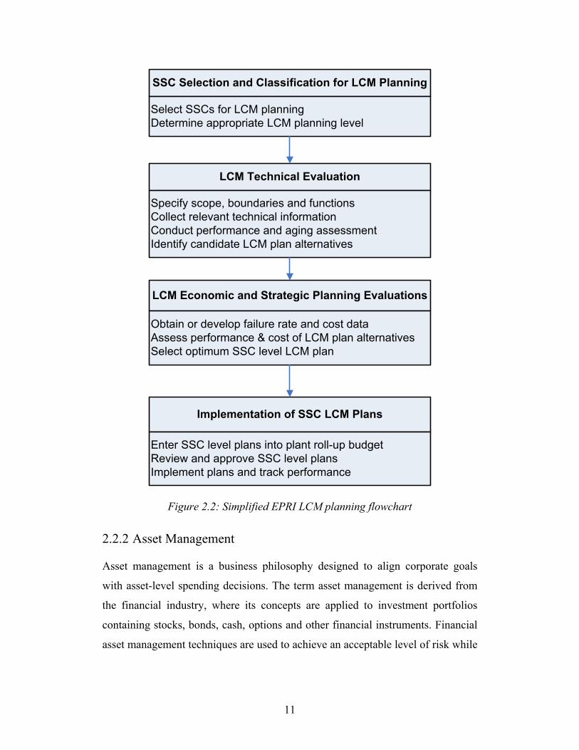
The LCM planning process consists of four main stages, as shown in Figure

2.2. The first stage is the selection of SSCs important to plant safety, reliability,

and economics. EPRI (2001) suggests several formal approaches in evaluating

and ranking important SSCs for nuclear power plants. Once important SSCs are

identified, depending on the level of criticality, LCM plans are developed for each

level of SSCs. The LCM planning flow chart in Figure 2.2 shows the activities

involved in each stage of the process.

Before conducting an aging assessment, the scope and functions of the SSC

are defined. This information is required to plan for alternative aging management

strategies to meet the scope and functions of SSC. The next step is to gather

relevant technical information related to plant performance and operating history

and review past and current maintenance plans. Using the technical information

gathered, an aging assessment is conducted on the SSCs, and alternate LCM plans

are identified. The relevant cost and failure rate data are obtained to assess the

performance and costs of each alternative LCM plan. Planned and unplanned

costs are taken into account to evaluate the economic value of each alternative

LCM plan. Finally, an optimum SSC LCM plan is selected based on the level of

safety, reliability and economics over the life of the facility. The optimum LCM

approach is a function of the projected life of the facility. If the target life is not

specified, then an economic analysis must be performed over a range of facility

life options.

11

SSC Selection and Classification for LCM Planning

Select SSCs for LCM planningDetermine appropriate LCM planning level

LCM Technical Evaluation

Specify scope, boundaries and functionsCollect relevant technical informationConduct performance and aging assessmentIdentify candidate LCM plan alternatives

LCM Economic and Strategic Planning Evaluations

Obtain or develop failure rate and cost dataAssess performance & cost of LCM plan alternativesSelect optimum SSC level LCM plan

Implementation of SSC LCM Plans

Enter SSC level plans into plant roll-up budgetReview and approve SSC level plansImplement plans and track performance

Figure 2.2: Simplified EPRI LCM planning flowchart

2.2.2 Asset Management

Asset management is a business philosophy designed to align corporate goals

with asset-level spending decisions. The term asset management is derived from

the financial industry, where its concepts are applied to investment portfolios

containing stocks, bonds, cash, options and other financial instruments. Financial

asset management techniques are used to achieve an acceptable level of risk while

12

maximizing expected profits. Many techniques of financial asset management are

applicable to infrastructure asset management.

Today, the power industry is divided so that generation, transmission, and

distribution are run as separate businesses. To resolve issues like slow load

growth, aging equipment, depleting rate bases, rate freezes, and regulatory

uncertainties, the power sectors are exploring ways to increase earnings, credit

ratings and stock price. As the power industry is asset intensive, asset

management is considered as an effective way of improving conditions in these

fundamental areas.

In asset management, decisions are made to maximize profits and

performance by effectively managing risks and reducing capital spending. The

framework for asset management as described by Brown and Spare (2004) is a

process of concern to the asset owner, asset manager and service provider. The

asset owner sets the business values, corporate strategy, and corporate objective in

terms of cost, performance, and risk. The asset manager identifies the best way to

achieve these objectives and lays a multi-year asset plan. The service provider

executes the plan efficiently, and feeds back asset and performance data into the

asset management process.

Effective asset management strategies can be achieved by the prudent

understanding of and accounting for various uncertainties and risks. The risk from

various sources should be quantified so as to develop strategies that can reduce

uncertainties. Asset management is applied to both physical components and

financial components (EPRI, 1998). Physical asset management focuses on

uncertainties in equipment performance, maintenance, and operations. The

operations and maintenance of aging components is monitored through aging

management in such a way as to maintain safety and minimize life cycle costs.

The financial asset management concerns uncertainties in market prices, cost

estimates, discount rates, and various regulations in order to increase revenue,

reduce costs, and minimize risks.

13

2.2.3 Aging Management

Aging management is a part of LCM that is concerned with operations and

maintenance actions to control aging of equipment and performance with the aim

to maintain safety and minimize life cycle costs. Aging management involves

major decisions on equipment repair, replacement, and the consequences for

equipment failure or outage that results in substantial investments. To make such

decisions effective, quality data on equipment condition and proper aging

assessments are needed.

Maintenance is a part of the overall concept of asset management. Its goal is

to increase the duration of useful component life and postpone failures that would

require expensive repairs. Maintenance involves costs, and this fact is taken into

account in choosing the most cost-effective policy. The costs of maintenance are

balanced against the benefits from increased performance or reduced risks.

Details of maintenance polices and the present polices in the electric power

industry are discussed in a paper by IEEE Task Force (2001).

The importance of maintenance has been growing over the years. In this

modern era of mechanization and automation, maintenance plays a vital role and

is the largest department in any organization. In fact, maintenance is becoming an

important part of asset management (Endrenyi, et al., 2001). The sophistication of

equipment has increased the impact of unplanned downtimes caused by system

failures. Today, the impact of system downtimes is unacceptably high and has to

be reduced with proper maintenance planning. By performing little maintenance,

system performance is reduced and may result in costly system failures. On the

contrary, if maintenance is increased, system performance could increase, but the

cost of maintenance will be high.

A maintenance model is a mathematical model by which both costs and

benefits of maintenance are quantified and by which an optimum balance between

both of them is achieved. Often norms have to be set to define failure and the

benefits of maintenance, and therefore they are more difficult to quantify. In this

case, one has to minimize maintenance costs in order to meet these norms. The

14

maintenance objectives as summarized by Dekkar (1996) are aimed at ensuring

system function; ensuring system life; ensuring safety; and ensuring human well-

being.

2.3 Technical Methods Needed to Support LCM

2.3.1 Overview of Maintenance Practices

The early application of maintenance management dates back to the 1950s and

60s. At that time, maintenance actions were mainly predefined activities carried

out at fixed intervals called scheduled maintenance. These were meant to reduce

system failures and unplanned system downtime. However, such a maintenance

policy may be quite inefficient as it may be costly in the long run (Barlow and

Proschan, 1965) and may not greatly extend system lifetime. In the 70s condition

monitoring came forward, focusing on techniques which predict failures using

information on the actual state of the equipment (predictive maintenance)

(Mobley, 2002, Makis et al., 1998, Barata, et al., 2002, Jardine, et al., 1999). This

approach proved to be more effective than scheduled maintenance. Detailed

studies about the failure of equipment created a better understanding of failure

mechanisms, resulting in better designs. But such applications are not popular in

decision-making analysis (Dekkar, 1996).

The key approach popular in industry is the Reliability Centred Maintenance

(RCM) (Moubray, 1997). In an RCM approach, various alternative maintenance

policies can be compared and the most cost-effective for sustaining equipment

reliability is selected (Vatn et al., 1996). It can be regarded as the more qualitative

approach to maintenance, in which optimization models are quantitative approach.

However, this approach is more heuristic and needs expert judgment at various

steps. The reason various models are being proposed in the literature is to aid the

maintenance scheduling, depending on the problem.

Several maintenance models are discussed in the literature (Barlow and

Proschan, 1965, Dekkar, 1996, Endrenyi, 2001). The most popular maintenance

models are discussed here.

15

2.3.1.1 Corrective Replacement

Corrective replacement is a simple and straightforward policy; when a component

fails it is replaced by a new one or repaired to working condition. This technique

is often called reactive maintenance or corrective maintenance (Mobley, 2002).

No maintenance task is needed till the system fails, which means no money is

spent on maintenance. The maintenance staff must be prepared for the any type of

failure, which may be anything from replacing a few components to a complete

overhaul. The major expenses associated with this type of maintenance are high

inventory cost, high overtime labour cost, high machine downtime, and low

production availability. However, this technique results in high maintenance costs

in the long run and lower system availability.

2.3.1.2 Age Replacement and Block Replacement policy

In age replacement policy, the system is replaced either at a certain age or when it

fails, whichever comes first. In block replacement policy, the system is replaced

either at fixed intervals or when the system fails. These methods are extensively

discussed in the literature and are still practiced. The optimal age replacement is

more profitable than the optimum block replacement. But when the emergency

failure costs are the same, the cost of a preventive maintenance carried out at

preplanned time, as in block replacement, will be smaller than the corresponding

preventive maintenance for age replacement (Gertsbakh, 2000).

2.3.1.3 Minimal Repair Policy

In the minimal repair policy technique, the system is subjected to minimal repair

when the system fails, and replacements are done at fixed intervals. This method

is different from block replacement, whereby the system is repaired when failure

occurs (Vatn et al., 1996). It is commonly assumed that the system after

preventive maintenance is either as good as new (perfect maintenance) or as bad

as old (minimal maintenance). In reality, these assumptions are not particularly

true, so such maintenance actions are termed imperfect maintenance (Mettas and

Zhao, 2005). Minimal repair or imperfect maintenance actions restore the system

16

to an operating state, but there is also a risk of failure or outage in future

operation. This policy may be prudent when there is a need to postpone relatively

high refurbishment policy in order to extend the useful life.

2.3.1.4 Predictive maintenance

In preventive maintenance, maintenance is carried when needed. The need for

maintenance is established through periodic or continuous inspection. To perform

meaningful periodic inspections, diagnostic routines and techniques are required

to help identify disorders that call for maintenance (Mobley, 2002). The aging

mechanisms are identified from periodic or continuous inspection to understand

the extent of degradation and use proper mechanistic or probabilistic models to

predict the future state of degradation. This approach may suggest the right

preventive maintenance action when needed. Predictive maintenance could be a

cost effective alternative when it is correctly implemented. If the consequences of

equipment failure are high and when the periodic inspection is feasible and less

costly, predictive maintenance may result in a cost-effective alternative.

2.3.1.5 Periodic Inspection

Commonly used diagnostic methods include visual inspection, optical inspection,

neutron analysis, radiography, eddy current testing, ultrasonic testing, vibration

analysis, lubricant analysis, temperature analysis, magnetic flux leakage analysis,

and acoustic emission monitoring. Each of these methods has advantages and

limitations.

In some cases, when periodic inspection cannot reveal the actual status of the

equipment or when it is not feasible to conduct periodic inspection, condition

monitoring is preferred. When the cost of implementing condition monitoring is

not excessive, this method proves to be more economical than maintenance based

on regular inspection.

Other maintenance models discussed in the literature are total predictive

maintenance (TPM) and reliability centered maintenance (RCM) (Dekkar, 1996,

Mobley, 2002). TPM was developed by Deming in the late 1950s, which is meant

17

to improve system effectiveness. RCM is based on regular assessments of

equipment condition; it involves system analysis like FMEA (Failure Mode and

Effect Analysis) and an investigation on system operating needs and priorities.

Maintenance models are classified according to the deterioration model

(Dekkar, 1996).

1. Deterministic Models

2. Stochastic Models

A. Under Risk

B. Under Uncertainty.

The deterioration process is represented by a sequence of stages of increasing

wear, finally leading to system failure. Deterioration is of course a continuous

process, and only for the purpose of easier modeling may it be considered in

discrete steps. The difference between risk and uncertainty is that risk assumes

that the probability distribution of the time to failure is available, which is not so

for uncertainty. In some models, system failure can occur not only because of

excessive degradation, which leads to critical state of the system, but also because

of random shocks which suddenly fail the system and whose occurrence

probability is degradation dependent. These models are often solved using

Markov or semi-Markov models (Smilowitz and Madanat, 2000, Barata et al.,

2002) and Gamma process models (Yuan et al., 2006, Frangopol et al., 2004). The

probabilistic modeling of degradation mechanisms and the effects of maintenance

on equipment performance and life cycle costs demand effective LCM.

2.3.2 Current Probabilistic Asset Management Practices

Traditionally, the electric power utilities employed preventive maintenance

programs to keep their assets in good condition as long as the process was

economical. Given the present economic constraints, an efficient maintenance

program has become an important part of asset management. Various electric

power organizations in different countries have begun to implement asset

18

management to meet the demands of the present market (Brown and Spare, 2004,

Morton, 1999, Endrenyi et al., 1998, Bertling et al., 2005). This has recently led to

the development of various asset management frameworks and supporting

models.

In power distribution systems, two methods are developed to address the

effect of maintenance on system reliability (Endrenyi et al., 2004), namely RCAM

(Reliability Centered Asset Maintenance) and ASSP (Asset Sustainment Strategy

Platform). Both approaches analyze the choice of a component maintenance

policy in a system context. The activities involve system reliability evaluation,

prioritization of component maintenance based on component criticality, effect of

various component maintenance policies on system reliability, and life cycle costs.

It is said that the conventional RCM (Reliability centered Maintenance) is

generally not capable of showing the benefits of maintenance for system

reliability and costs (Bertling et al., 2005).

2.3.2.1 RCAM (Reliability Centered Asset Maintenance)

The RCAM method is developed for asset maintenance in electric power

distribution systems (Bertling et al., 2005). In this method, the failure events are

assumed to occur randomly, and therefore the models are based on probability

theory. A network modeling technique is applied to calculate system reliability by

the minimal cut set approach. A computer code RADPOW (reliability assessment

of electric distribution systems) is used to calculate system reliability and

sensitivity of the components. For the components which are critical, preventive

maintenance (PM) strategies are laid out, and the effects of PM and the economic

analysis are modeled by another program code. These two modules interact with

each other to assist in arriving at a cost-effective maintenance strategy.

The failure rate is assumed to be constant, which is an assumption reasonable

for most electrical components but may not be applicable for components with

continuous degradation. The effect of maintenance action is modelled by reducing

the failure rate, to study its impact on overall system reliability.

19

2.3.2.2 ASSP Approach (for Asset Sustainment Strategy Platform)

The ASSP approach is somewhat similar to RCAM and includes several programs

which interact as necessary. The reliability evaluation and sensitivity analysis is

performed by programs REAL and WinAREP (Endrenyi et al., 2004); the critical

components are ranked and maintenance alternatives are investigated. The effect

of maintenance is carried out using programs AMP (based on Markov model

which accounts for deterioration with ageing) (Endrenyi et al., 1998) and first

passage times FPT (the mean times of failure from any state in the AMP model)

(Anders and De Silva, 2000). To include the associated costs of maintenance, the

ASSP platform includes a program called RiBAM (Risk Based Asset

Management). RiBAM (Anders et al., 2001) uses the information from AMP and

FPT to construct life curves and cost curves by which cost optimization can be

performed.

The Markov model for deterioration is a reasonable conceptual model to

determine the effect of maintenance. Collecting data periodically on a component

condition is not always practical in actual field inspections. The estimation of

transition probabilities in such a model is difficult from field inspection data.

Hence, in such cases the transition probabilities are usually assumed to reflect the

model estimates from experience and past data.

2.3.2.3 Application to Power Infrastructure Systems

The concept of asset management was introduced recently in the power industry.

Most of the articles on asset management talk about the scope and advantages of

the asset management approach in transmission and distribution (Brown and

Spare, 2004, Butera, 2000, Morton, 1999, Chan, 2004, Wernsing and Dickens,

2004). Development of probabilistic models for the asset management of

distribution network has been recently attempted by Endrenyi et al., (2004). Some

results on the application of asset management techniques in power distribution

systems are discussed here.

An asset management of wood pole utility structures (Gustavsen and

Rolfseng, 2004) is discussed by predicting the pole replacement rate and

20

considering the stochastic variation in pole strength and climate loads. The paper

describes the probabilistic approach for evaluating the economic impact of

alternate maintenance strategies, design strategies, and compensation fees for

undelivered energy. The life prediction and inspection practice for aging wood

poles is also discussed (Li et al., 2004). The inspection on aging poles is based on

the current condition of poles and acceptable pole replacement rate for older poles.

The feasibility of the RCAM approach for circuit breakers is discussed

(Lindquist et al., 2004). From the statistics collected on circuit breaker failures

and sub-components, the failure rates are estimated. A probabilistic approach

based on the condition of the circuit breaker and different levels of maintenance is

proposed (Natti et al., 2004). The failure, repair and maintenance sequences are

described as Markov processes, and optimal maintenance intervals are discussed.

2.3.2.4 Application to Civil Infrastructure Systems

In the construction industry, operation, maintenance, repair and renewal of assets

represents a major growing cost in North America (Vanier, 2001). The assets

range from complex interrelated underground networks to sophisticated buildings

and roadway systems. Many major asset owners in North America now recognize

the importance of knowing the current and future states of their infrastructures.

Asset management plays an important role in maintaining the assets to optimize

expenditure and maximize the value of the asset over its lifecycle. Managers of

municipal infrastructures are realizing the need for effective tools and strategies to

manage the large asset base.

Application of life-cycle management in civil engineering infrastructures is

used in rehabilitation/construction alternatives in pavements (Salem et al., 2003)

and bridges (Kong and Frangopol, 2003).

2.4 Discussion

Most of the asset management models discussed in the literature are conceptual in

nature and do not solve the practical difficulties in modeling the lifetime of the

21

equipment. The models described in Section 2.3.2 are prescriptive and do not

consider life data obtained from field inspections.

The equipment in energy infrastructure experience degradation and the

consequences of equipment failure from such degradation are high. This reality

has led to the need for evaluation methods for fitness for service assessment of

equipments. In the nuclear industry, the assessment of the conditional

probabilities of tube failures, leak rates, and ultimately risk of core damage or of

exceeding site dose limits is an approach to equipment fitness-for-service

guidelines that has been used increasingly in recent years. The advantage of

probabilistic analysis is that it avoids the excessive conservatism typically present

in deterministic fitness-for-service guidelines (Harris et al., 1997). Probabilistic

modeling of steam generator tube degradation is typically done only when the

level of degradation is such that using normal deterministic fitness-for-service

guidelines would result in the number of tube repairs being sufficiently large to

affect the power generation capability of the affected unit.

Development of probabilistic models from inspection data recorded from

plant outages will allow great confidence in assessing remaining life and in

ensuring an extended operating life. The literature is deficient in information on

the practical applications in developing probability models from partial inspection

studies.

The rest of this thesis attempts to develop probabilistic models based on

inspection data. Development of realistic probability models is crucial for making

credible life cycle management decisions.

22

CHAPTER 3 LIFETIME DISTRIBUTION MODELS

3.1 Introduction

The estimation of lifetime distribution is essential in managing aging equipment

through a systematic risk based approach. The lifetime distribution of equipment

is a key input to maintenance models and life cycle cost optimizing models. These

models are used to quantify the effect of various maintenance actions on the

equipment performance and associated costs over equipment lifetime. The

estimation of lifetime distribution hence plays a crucial role in a credible life

cycle management models.

Various equipments in civil and energy infrastructures are designed with

relatively high lifetime and hence the time needed to observe such high lifetimes

is not practical. Continuous inspection on equipment lifetimes may not be a cost

effective alternative and hence periodic or non-periodic inspections are performed

and in some cases there are no inspections. Inspections are mostly affected by the

safety of the equipment, economics, and accessibility. Such situations often

results in incomplete observations on equipment lifetimes. Due to increasing

awareness of the impact of aging equipment has alerted some utilities recently to

inspect the whole population for the first time creating a snap shot situation on the

population lifetimes.

Incomplete observations cannot be ignored as they provide vital information

on equipment lifetimes. Such incomplete observations pose challenges in both

estimating and in terms of interpreting lifetime distribution models. This chapter

discusses various types of incomplete observations and statistical tools to deal

with incomplete lifetimes in estimating realistic lifetime distribution models.

23

3.2 Types of Data

3.2.1 Background

To asses the condition of equipment in its current state and to predict its future

state needs information on its operating characteristics in its service. Various

inspection techniques are being used to monitor (periodically or continuously) the

operating state of the equipment. The objective of inspection can vary depending

upon the type of equipment and its criticality. Inspection techniques range from

simple visual inspection to sophisticated Non Destructive Testing (NDT)

depending on the economics and safety factors. The scope of data collection

(inspection) is related to the scope of analysis to be performed on equipment over

its lifetime. Depending on the scope of inspection, the observations could be

lifetimes of equipment or events over lifetime.

For example in the case of wood poles, utilities have adopted the

measurement of the minimum remaining shell thickness of wood pole at the

ground level as an indicator of pole condition. The shell thickness can be reliably

estimated using the Resistograph. Typically, a pole is considered to be at the end

of service life when its minimum shell thickness is reduced to less than 2 inches

(Newbill, 1993). Such a pole is referred to as a substandard pole, which has a

higher risk of failure under an adverse environmental overloading. The age at

which a pole reaches the substandard condition is designated as the end of life

(EOL). One of the applications discussed in this chapter is based on the wood

pole inspection data collected by a utility.

The condition of steam generator of a nuclear power plant is assessed by

means of eddy current inspection of steam generator tubes during outages. The

objective of eddy current inspection is to monitor various degradation

mechanisms and characterize the defects during outages. In case of pitting

corrosion degradation, the number of corrosion pits and depth of pits are observed

at each outage. The extent of degradation which is characterized by the pit

generation and pit depth defines the service life (lifetime) of the steam generator.

24

In such cases there is a need to quantify the uncertainties in observing inspection

data.

Observations may be done differently depending on factors such as the time

needed to observe events that define equipment state, the feasibility of following

equipment over time, and the mechanism for recording relevant data on

equipment condition. Such factors create situations where the observations are

censored, truncated, and categorical. The information on such observations should

be carefully accounted in order to reliably asses/model the equipment

characteristics.

This section deals with the conceptual modeling of inspection data

encountered in practices that are accounted for in the statistical modeling of

lifetimes. Firstly a standard data analysis is described to estimate the lifetime

distribution given a sample of complete lifetimes. Then a distinction is drawn

between the standard case and the realistic case of censored inspection data

collected by electrical utilities.

3.2.2 Complete Lifetime Data

Complete lifetimes of components are obtained from such follow up studies. The

standard method of estimating the lifetime distribution is based on the cohort

analysis technique (Elandt-Johnson and Johnson, 1999). In an ideal analysis a

single cohort of in-service components is monitored regularly over a long span of

time until all the components reach the end of life. As an illustration, Figure 3.1

shows components installed in a particular year (say 1970) continuously followed

until the entire cohort ceases to exist. It is also referred to as a “longitudinal

survey” in health sciences and demography literature (Lawless, 2003, Keyfitz,

1985). Statistical analysis of such data is quite simple which is shown in Section

3.3.3.

25

1960 - 1970 1970 - 1990 1990 - 2000 2001 2002

Complete Lifetime

Start Endt

Figure 3.1: An ideal cohort data of complete service lifetimes

This approach is ideally suitable for components of low cost and short life

span. However, a complete sample of lifetime data from a single cohort of wood

pole is not easy to obtain. The reason is that it requires continuous follow up

inspection and assessment of a large number of poles from their installation over a

long service life (40 – 70 years), which is a costly and impractical undertaking.

Such issues are common in most of the high lifetime components of power

utilities.

3.2.3 Complete and Right Censored Lifetime Data

It is a refinement of the previous model by including in the analysis the

components that were found to be under good condition. The remaining lifetime

of components that are fit for service at the time of inspection is unknown; and it

is referred to as right censored lifetime data.

26

Group 1Complete Lifetime

1950 - 1960 1970 - 1980 1990 - 2000 2001 Inspection2002

Group 2Right Censored Lifetime

Figure 3.2: Inclusion of right censored lifetimes

Figure 3.2 shows the conceptual representation of a typical inspection data

under this model. The sample can be divided into two groups of complete and

right censored lifetime data. Consideration of right censored data is important for

a realistic estimation, since they contain valuable information about an improved

prospect of future survival. Therefore, an omission of such data from statistical

analysis could lead to an underestimation of life expectancy, as shown in Section

3.4.1.

3.2.4 Interval and Right Censored

This is the most realistic model that mimics the periodic or non-periodic

inspection data available from the power utility industry. In some cases the

failures are not self announcing and can only be revealed from inspection. Such

situations result in interval censored observations where only information

between inspections is recorded. The statistical analysis of interval censored data

is not straight forward but can be estimated by likelihood methods as discussed in

section 3.3.4.

27

Group 1Interval Censored

1950 - 1960 1970 - 1980 1990 - 2000 2001 Inspection2002

Group 2Right Censored

Interval Censored Lifetime

Start End SubstandardState

c

Figure 3.3: A mixed cohort data with interval censored lifetimes (c = censoring

interval)

The available data on wood poles provide a single snap shot of pole

population taken at the time of inspection in year 2002, as shown in Figure 3.3.

The data consist of two groups: (1) right censored lifetimes, and (2) a small

fraction of substandard poles, and their exact time of reaching the end of life is

not known. The situation is analogous to cross-sectional surveys used in health

impact assessment (Elandt-Johnson and Johnson, 1999, Lawless, 2003).

The substandard pole data is treated as interval censored lifetimes, rather than

considering them as complete lifetimes. The reason for assuming interval

censoring is that the wood degradation is a fairly slow and intermittent process.

The fungal decay continues only under favourable environment (humidity and

temperature), otherwise it remains dormant. Also, reaching the substandard state

does not result in an immediate pole failure. The reason is that poles are

conservatively designed and wood is subject to low stresses under normal service

conditions. The pole failure is typically caused by an extreme weather event.

28

Therefore, substandard poles may remain in-service for many years, until detected

by an inspection. Because of this, the time of detection cannot be construed as the

actual end of service life.

3.2.5 Current Status Data

This is a special case of interval censored model where the censoring interval is

completely unknown. The censoring interval c in Figure 3.3 is the age of the

component, such type of observation is also referred to as left censored data.

Current status observations are common from cross sectional survey of

population. The component has either failed at some point of time from the start

of its service or either survived at the time of inspection. Such observations

introduce greater uncertainty in estimating the lifetime of the components. The

statistical estimation of current status data is complicated and can be estimated by

likelihood methods discussed in Section 3.3.3.4.

3.3 Lifetime Data Analysis

In order to improve or make any decisions on a system performance, the decision

maker needs to have an idea on how the system behaves in its lifetime.

Information on the system can be known from data on system monitoring or on

system test data or on expert opinion. These lifetime data can be modelled with

suitable mathematical expressions. This information is helpful in quantifying the

system lifetime, which in turn helps in developing models which can improve the

system performance.

The definition of lifetime includes a time scale and time origin, as well as

specification of event that determines the lifetime. The commonly used models

for lifetime estimation can be classified as fully parametric, non-parametric and

semi parametric (Lawless, 2003, Cox and Oakes, 1984, Nelson, 1982). This

section discusses the estimation techniques to model the lifetime data using

illustrations from various inspection methods.

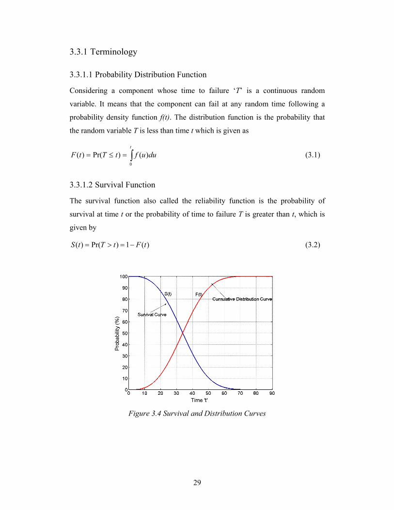
29

3.3.1 Terminology

3.3.1.1 Probability Distribution Function

Considering a component whose time to failure ‘T’ is a continuous random

variable. It means that the component can fail at any random time following a

probability density function f(t). The distribution function is the probability that

the random variable T is less than time t which is given as

∫=≤=t

duuftTtF0

)()Pr()( (3.1)

3.3.1.2 Survival Function

The survival function also called the reliability function is the probability of

survival at time t or the probability of time to failure T is greater than t, which is

given by

)(1)Pr()( tFtTtS −=>= (3.2)

Figure 3.4 Survival and Distribution Curves

30

As shown in Figure 3.4, the point at which both curves meet is the median

value time t50. The Mean time to failure (MTTF) for the component (mean

lifetime / life expectancy) is defined as

∫∞

=0

).(. dttftμ (3.3)

By applying integration by parts, it can show that the MTTF can be expressed

as the area under the survival curve. The expression for MTTF in terms of

survival function is given as

∫∞

=0

).( dttSμ (3.4)

Figure 3.5 shows survival plots for two components with equal MTTF and

different variance. Component 2 has lower variability than component 1 in time to

failure distribution.

Figure 3.5 Survival curves for two components

3.3.1.3 Hazard Function

Hazard rate can be defined as the conditional failure probability of the component

given that it has survived up to time t. The hazard rate is expressed as

31

ttTttTtth

t Δ>Δ+≤<

=∞→Δ

)/Pr(lim)( (3.5)

The hazard rate is also called instantaneous failure rate (or age specific

failure rate). By definition of density function and survival function the hazard

function follows

)()()(

tStfth = (3.6)

The cumulative hazard is integrated summation of hazard probabilities as

time increases which is expressed as

∫=t

dtthtH0

).()( (3.7)

The expressions h(t), f(t), S(t), H(t) can be derived by knowing any one of the

expressions.

For example, conducting a test on the failure of N similar components and

keeping track of failures with time. The survival distribution and hazard estimates

can be given as

Nm

tF ii =)(ˆ (3.8)

)(ˆ1)(ˆii tFtS −= (3.9)

)()()(ˆ

i

ii tN

tdth = (3.10)

N → Total number of components mi → Number of components failed until time ti d(ti) → Number of components failed exactly at time ti N(ti) → Number of components survived at time ti The relationship between the probability functions is shown in the table below

32

Table 3.1 Relationship among probability functions

)(th )(tf )(tS )(tH

)(th -/- ∫−

= t

dxxf

tfth

0

)(1

)()(

)(

)()(

tS

tSdtd

th⎟⎠⎞

⎜⎝⎛−

= )()( tH

dtdth =

)(tf ⎥⎦

⎤⎢⎣

⎡−= ∫

t

dxxhthtf0

)(exp)()( -/- )()( tSdtdtf −= [ ])(exp)()( tHtH

dtdtf −⎟

⎠⎞

⎜⎝⎛=

)(tS ⎥⎦

⎤⎢⎣

⎡−= ∫

t

dxxhtS0

)(exp)( ∫−=t

dxxftS0

)(1)( -/- [ ])(exp)( tHtS −=

)(tH ∫=t

dxxhtH0

)()( ⎥⎦

⎤⎢⎣

⎡−−= ∫

t

dxxftH0

)(1log)( [ ])(log)( tStH −= -/-

There exists a variety of models which can be used in lifetime distributions,

for example, exponential, Gaussian, Extreme value, Gamma etc (Lawless, 2003,

Kalbfleisch and Prentice, 2002). The widely used model in engineering

application is Weibull which is discussed in the next section.

3.3.2 Parametric Distributions

3.3.2.1 Weibull Distribution

The Weibull distribution is the most popular choice in the survival analysis with

the survival and hazard rate functions given as

⎪⎭

⎪⎬⎫

⎪⎩

⎪⎨⎧

⎟⎠⎞

⎜⎝⎛−=

β

αttST exp)( and

1

)(−

⎟⎠⎞

⎜⎝⎛=

β

ααβ tth (3.11)

where scale and shape parameters are denoted by α >0 and β>0, respectively. The

hazard decreases for β<1 and increases for β>1 whereas for β=1 Weibull

distribution is an exponential with constant hazard rate. The hazard rate curves for

various values of shape parameter in a sample case are shown in the Figure 3.6.

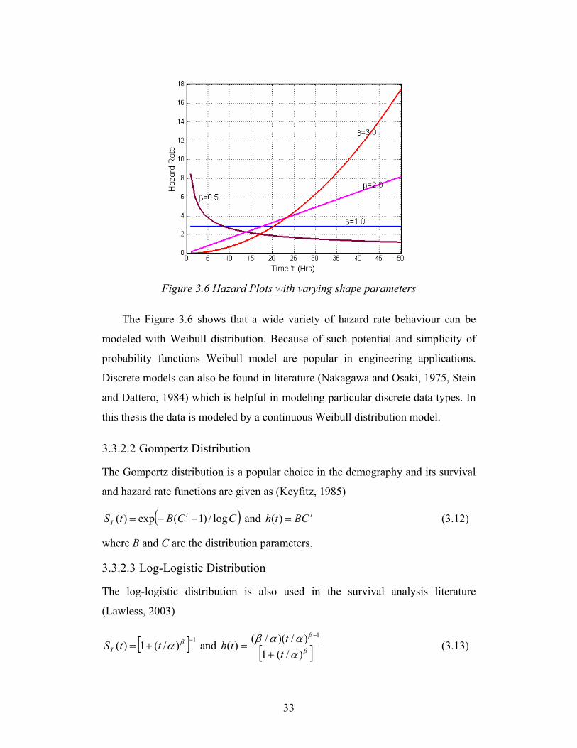
33

Figure 3.6 Hazard Plots with varying shape parameters

The Figure 3.6 shows that a wide variety of hazard rate behaviour can be

modeled with Weibull distribution. Because of such potential and simplicity of

probability functions Weibull model are popular in engineering applications.

Discrete models can also be found in literature (Nakagawa and Osaki, 1975, Stein

and Dattero, 1984) which is helpful in modeling particular discrete data types. In

this thesis the data is modeled by a continuous Weibull distribution model.

3.3.2.2 Gompertz Distribution

The Gompertz distribution is a popular choice in the demography and its survival

and hazard rate functions are given as (Keyfitz, 1985)

( )CCBtS tT log/)1(exp)( −−= and tBCth =)( (3.12)

where B and C are the distribution parameters.

3.3.2.3 Log-Logistic Distribution

The log-logistic distribution is also used in the survival analysis literature

(Lawless, 2003)

[ ] 1)/(1)( −+= βαttST and [ ]β

β

αααβ)/(1)/)(/()(

1

ttth

+=

−

(3.13)

34

The life expectancy is simply the area under the survival curve, i.e.,

∫∞

=0

)( dxxSm TT (3.14)

3.3.3 Non-Parametric Lifetime Distribution

3.3.3.1 Complete Data

In the first model as discussed in Section 3.2.2, a sample of complete lifetime data

is considered for the analysis. The sample consists of di entries of age ti, i = 1, N,

and the sample likelihood is given as

{ }∏=

=N

i

diT

itfL1

)( (3.15)

where fT(t) is the probability density of the lifetime distribution. In other words,

the sample likelihood is proportional to the probability that the data comes from

the model fT(t). Assuming an analytical distribution function (e.g. Weibull

distribution), its parameters can be estimation by maximizing Eq.(3.15).

An empirical (sample based) survival curve, ST(t), can be analytically derived

considering that lifetimes are recorded as a discrete variable taking values t1 <

t2< …< tN. The probability density at age ti can be estimated as

)()()( 1+−= iTiTi tStStf and it is related to the hazard rate as )()()( iii tSthtf = .

Combining these relations leads to a recursive equation of survival curve.

{ })(1)()()()()()()( 11 iiiiiiii thtStStStStSthtf −=⇔−== ++ (3.16)

Finally, the discrete survival curve can be written in terms of hazard rate as

[ ]∏−

=

−=1

1

)(1)(i

kkiT thtS (3.17)

Using Eqs.(3.16) and (3.17), the likelihood function can be written in terms

of the hazard rate, and maximizing the log likelihood with respect to the hazard

rate, h(ti), leads to a non-parametric estimate as

35

)()(

i

ii tm

dth = (3.18)

where m(ti) = the cumulative number of components surviving beyond the age ti,

i.e.,

∑+=

=N

ikki dtm

1

)( (3.19)

3.3.3.2 Complete and Right Censored Lifetime Data

This model also considers the right censored lifetimes observed in the inspection

data. The censoring time corresponds to the age at the time of inspection.

Considering in an age group ti, the sample consists of di complete lifetimes and (ni

- di) right censored lifetimes, the likelihood function is given as

{ } { }∏=

−=N

i

dniT

diT

iii tStfL1

)()( (3.20)

Again using Eqs.(3.16) and (3.17), the likelihood function is written in terms

of the hazard rate, and maximizing the log likelihood leads to a non-parametric

estimate of the hazard rate at age ti similar to that given by Eq.(3.18). However, in

this case the cumulative number of components surviving beyond the age ti is

estimated as

∑=

=N

ikki ntm )( (3.21)

Kaplan and Meier (1958) first derived this non-parametric (or product limit)

estimator of the survival function.

3.3.3.3 Interval and Right Censored Lifetime Data

In this model, the complete lifetimes are replaced with the interval censored

values. The likelihood function for a sample with di interval censored and (ni - di)

right censored lifetimes in the age group ti, is written as

{ } { } iiji dniT

N

i

diT tScTtFL −

=∏ >= )()|(

1

(3.22)

36

where c denotes the censoring interval and FT(t) is the cumulative lifetime (T)

distribution. Note that the conditional distribution, used to account for the

censoring of observed lifetimes, is given as

)()(1

)()(1)](|[1)](|[

ctStS

ctTPtTPctTtSctTtF

T

TTT −

−=−≥

≥−=−>−=−> (3.23)

Now the conditional survival probability in Eq.(3.23) can be written in a discrete

form using Eq.(3.17) as

[ ]

[ ][ ]∏

∏

∏−<≤−−

−−

=

−

= −=−

−=

−=−>

111

1

1

1 )(1)(1

)(1

)()()](|[

ikcikci

kk

i

kk

iT

iTiiT

i

thth

th

ctStSctTtS (3.24)

Although the likelihood function can be written in terms of hazard rates using

Eq.(3.24), a simple analytical expression for the hazard rate estimator cannot be

derived. In such cases it is convenient to use parametric distribution models to

estimate survival probabilities.

3.3.3.4 Current Status Data

Estimation of non parametric estimates from current status observations as

discussed in Section 3.2.5 is not a straight forward task. However, the survival

function can be estimated by Maximum likelihood method as described below

(Turnbull, 1976, Meeker and Escobar, 1998). Considering the case of a cross

sectional study conducted on a component population in a particular year

resulting in a snap shot of condition data on the population.

Consider that the component population consists of age groups 10321 ,...,,, tttt

at the time of inspection as shown in Figure 3.7. For each age group the number

of components inspected ( in ) and the number of components in failed state ( id )

is known. Consider the interval failure probabilities ip in the population as

shown in Figure 3.7 for the observed data.

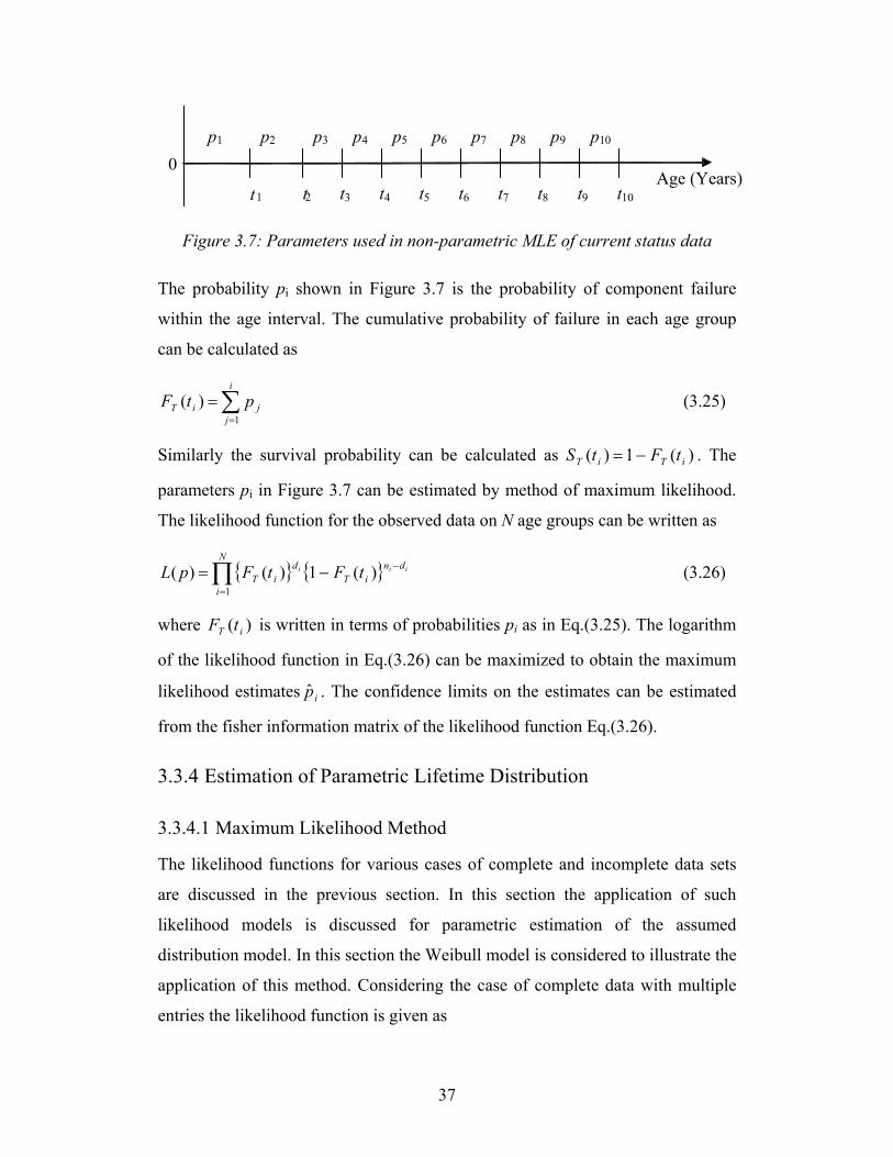
37

0

t 1 t 2 t 3 t4 t5 t6 t7 t8 t9 t1 0

p 1 p 2 p 3 p 4 p 5 p 6 p 7 p 8 p 9 p 1 0

Age (Years)

Figure 3.7: Parameters used in non-parametric MLE of current status data

The probability pi shown in Figure 3.7 is the probability of component failure

within the age interval. The cumulative probability of failure in each age group

can be calculated as

∑=

=i

jjiT ptF

1)( (3.25)

Similarly the survival probability can be calculated as )(1)( iTiT tFtS −= . The

parameters pi in Figure 3.7 can be estimated by method of maximum likelihood.

The likelihood function for the observed data on N age groups can be written as

{ } { }∏=

−−=N

i

dniT

diT

iii tFtFpL1

)(1)()( (3.26)

where )( iT tF is written in terms of probabilities pi as in Eq.(3.25). The logarithm

of the likelihood function in Eq.(3.26) can be maximized to obtain the maximum

likelihood estimates ip̂ . The confidence limits on the estimates can be estimated

from the fisher information matrix of the likelihood function Eq.(3.26).

3.3.4 Estimation of Parametric Lifetime Distribution

3.3.4.1 Maximum Likelihood Method

The likelihood functions for various cases of complete and incomplete data sets

are discussed in the previous section. In this section the application of such

likelihood models is discussed for parametric estimation of the assumed

distribution model. In this section the Weibull model is considered to illustrate the

application of this method. Considering the case of complete data with multiple

entries the likelihood function is given as

38

{ }∏=

=n

i

di

itfL1

)( (3.27)

Where di is the number of complete observations at time ti, n is the number of

instances of lifetimes observed. Considering lifetime distribution follows Weibull

model the likelihood function is given as

∏=

−

⎪⎭

⎪⎬⎫

⎪⎩

⎪⎨⎧

⎪⎭

⎪⎬⎫

⎪⎩

⎪⎨⎧

⎟⎠⎞

⎜⎝⎛−⎟

⎠⎞

⎜⎝⎛=

n

i

d

ii

i

ttL1

1

exp)(ββ

αααβθ (3.28)

where θ is the vector of the distribution parameters of the Weibull model. The

parameters are estimated by maximizing the likelihood function. To simplify the

numerical computation the natural logarithm of the likelihood is maximized to

estimate the distribution parameters. The logarithm of the likelihood function is

given as

∑∑∑===

−−+==n

iii

n

iii

n

ii tdtddLl

111

1)log()1()/log())θ(log()θ( β

φβφβ (3.29)

where φ is substituted for βα . Standard optimization algorithm can be used to

estimate the parameters by maximizing Eq.(3.29). Alternatively, the parameters

are found by solving the first partial derivatives of the likelihood function

Eq.(3.29) with respect to the parameter. The first partial derivatives of the log-

likelihood function can be written as

∑∑

∑∑∑

==

===

=+−=∂∂

=−+=∂∂

n

iii

n

ii

n

iiii

n

iii

n

ii

tddl

ttdtddl

12

1

111

011)θ(

0log1log1)θ(

β

β

φφφ

φββ (3.30)

39

0loglog11

1

1

11

1

1

=

⎟⎟⎟⎟

⎠

⎞

⎜⎜⎜⎜

⎝

⎛

−+

==

∑∑

∑∑∑

∑

∑

=

=

=

==

=

=

n

iiiin

iii

n

iin

iii

n

ii

n

ii

n

iii

ttdtd

dtdd

d

td

β

β

β

β

β

αφ

(3.31)

Solving Eqs.(3.31), the estimates for β̂ and α̂ are obtained. Likewise the

parameters of the selected distribution are estimated by maximizing the log-

likelihood function corresponding to the observed data.

For the case of complete and right censored, the likelihood function Eq.(3.20)

takes the following form

∏=

−−

⎪⎭

⎪⎬⎫

⎪⎩

⎪⎨⎧

⎟⎟⎠

⎞⎜⎜⎝

⎛⎥⎦⎤

⎢⎣⎡−

⎪⎭

⎪⎬⎫

⎪⎩

⎪⎨⎧

⎪⎭

⎪⎬⎫

⎪⎩

⎪⎨⎧

⎟⎠⎞

⎜⎝⎛−⎟

⎠⎞

⎜⎝⎛=

N

i

dn

i

d

ii

iii

tttL1

1

expexp)θ(βββ

ααααβ (3.32)

The likelihood function applicable to Interval censored along with right

censored observations is derived from Eq.(3.22) as

jjj dm

jN

j

d

jj ttctL

−

= ⎪⎭

⎪⎬⎫

⎪⎩

⎪⎨⎧

⎟⎟

⎠

⎞

⎜⎜

⎝

⎛⎥⎦

⎤⎢⎣

⎡−

⎪⎭

⎪⎬⎫

⎪⎩

⎪⎨⎧

⎟⎟

⎠

⎞

⎜⎜

⎝

⎛⎥⎦

⎤⎢⎣

⎡−⎥

⎦

⎤⎢⎣

⎡ −−=∏

βββ

αααexpexp1)θ(

1

(3.33)

The likelihood function for the case of current status data is similar to that

given in Eq. (3.33) where censoring interval 0=c .

For computational purpose, the logarithm of the likelihood (Eqs. 3.28, 3.32,

3.33) is maximized with respect to the distribution parameters (α and β) using a

standard MATLABTM optimization code (fminsearch and fminunc).

The Fisher information matrix is the expectation of the negative of the second

derivative of the log likelihood with respect to the parameters. Fisher information

is used to obtain asymptotic variance of the maximum likelihood estimator of the

distribution parameters (Kalbfleisch & Prentice, 2002). The asymptotic

40

covariance matrix of the maximum likelihood estimators is the inverse of the

Fisher information matrix.

1

ˆ,ˆ2

22

2

2

2

)()(

)()(

)ˆvar()ˆ,ˆcov()ˆ,ˆcov()ˆvar(

−

==

⎟⎟⎟⎟

⎠

⎞

⎜⎜⎜⎜

⎝

⎛

∂∂

−∂∂

∂−

∂∂∂

−∂∂

−=⎟⎟

⎠

⎞⎜⎜⎝

⎛

ααββαθ

αβθ

αβθ

βθ

ααβαββ

ll

ll

(3.34)

Using the asymptotic variance of the estimated parameters the approximate

confidence intervals can be obtained for the parameters estimated. A confidence

interval gives an estimated range of values which is likely to include the unknown

population parameter. Confidence interval is associated with confidence level

which gives the probability that the true value of the parameter lies within the

interval. The upper and lower bounds of the Weibull parameters are estimated as

⎟⎟

⎠

⎞

⎜⎜

⎝

⎛=

⎟⎟

⎠

⎞

⎜⎜

⎝

⎛=

β

βββ

β

β

ββ ˆ)ˆvar(

expˆ;

ˆ)ˆvar(

exp

ˆ k

kUL (3.35)

⎟⎟⎠

⎞⎜⎜⎝

⎛=

⎟⎟⎠

⎞⎜⎜⎝

⎛=

αα

αα

αα

ααˆ

)ˆvar(expˆ;

ˆ)ˆvar(

exp

ˆ k

kUL (3.36)

The bounds are derived based on lognormal approximation with confidence

level a, where )2/1(1 ak −Φ= − . For 95% confidence bounds (a=5%) on

parameter estimates, the value of k is 1.96. The variance of a function of

distribution parameters is estimated by delta method. The mean lifetime of

Weibull model is given as

⎟⎟⎠

⎞⎜⎜⎝

⎛+Γ=β

αμ 11T (3.37)

By delta method, the variance of mean lifetime is calculated as

( ) ( ) ( ) ( )βαβμ

αμ

ββμ

ααμ

μ ˆ,ˆcov2ˆvarˆvarvar22

⎟⎟⎠

⎞⎜⎜⎝

⎛∂∂

⎟⎠

⎞⎜⎝

⎛∂∂

+⎟⎟⎠

⎞⎜⎜⎝

⎛∂∂

+⎟⎠

⎞⎜⎝

⎛∂∂

= TTTTT (3.38)

41

Different types of parametric models can be applicable using likelihood

functions given in Section 3.3.3. One way to check for the best fit is by comparing

the parametric probability function plots with the non-parametric estimates.

Besides the graphical methods statistical tests are used to check the best fit model.

3.3.4.2 Test of Goodness of Fit

Models vary in complexity and assumptions, and it is necessary to check the

adequacy of the models. Although the probability plots are one of the tools to

check the models, they are not just sufficient to check some of the assumptions.

Hypothesis tests are most commonly used by statisticians to check the adequacy

of the models. The classical procedures (Lawless, 2003) to compare the

parametric models with non-parametric counterparts are Kolmogorov-Smirnov

Statistic and Cramer-von Mises Statistic. Such test statistics provide evidence for

or against the hypothesized model. Tests of fit for specific distributions (Lawless,

2003) like Weibull or Extreme are also available for complete and right censored

data.

Likelihood Ratio Statistic (LRS) is commonly used to compare different

models (Lawless, 2003, Nelson, 1982). LRS for testing null hypothesis (H0) Vs

alternative hypothesis (H1) can be given by

)ˆ(log2)ˆ(log2 01 θθ LL −=Λ (3.39)

Let the number of independent parameters in models H1 and H0 are m and n

respectively. Then under H0 and for large sample size Λ is approximately chi-

squared distribution ( 2nm−χ ).

3.3.4.2.1 Akaike Information Criterion (AIC)

In the absence of the true model it is difficult to compare models from tests

like LRS or other tests discussed above. On the other hand Akaike (1985) has

developed an information criterion (AIC) without specific reference to the true

model. Hence AIC can be useful in comparing different models. AIC is based on

entropy maximization principle (Akaike, 1985) which is the maximization of the

42

expected entropy of a true distribution with respect to the fitted predictive

distribution.

It is known that the maximum likelihood method leads to biased estimates of

the true parameters in case of finite sample data (Baker, 1990). Akaike derived an

unbiased estimator based on an information-theoretic interpretation of the

likelihood function. He proposed the following measure to test the goodness of fit

of an assumed model (Akaike, 1985):

KLAIC MAX 2]log[2 +−= (3.40)

where K is the number of distribution parameters and LMAX is maximum value of

the likelihood function under an assumed model. Among all candidate

distributions, the distribution that minimizes the AIC measure is considered as the

best fit distribution. The mathematical proofs are further discussed by Awad

(1996) and Cavanaugh (1997).

Since the AIC is on a relative scale that can range from a large negative to a

large positive limit, the AIC difference is a suitable basis to evaluate the goodness

of fit, which is calculated as

AICAICAIC ii min)( −=Δ (i = 1 - 3) (3.41)

where “min AIC” is the minimum value of the AIC measure among all the

distributions considered. For the best fit distribution, Δ(AIC) = 0.

3.3.5 Frailty Models

During lifetime data analysis among a collection of individuals it is assumed that

the lifetimes are independent. But there could be some unobserved risk factors

that are common between the individuals and constant over time. The frailty is the

term that describes the common risks acting as a factor on the hazard function.

Frailty model assume that all lifetime observations are independent given the

values of the frailty. This offers an advantage in interpretation of frailty as a

probability model, that is the conditional independence implies that dependence is

43

created by the common factors or the variation within individuals (Hougaard,

2000).

The unobserved risk within individuals is described by a random variable Y.

The hazard conditional on Y has the form.

)()|( 0 tYhYth = (3.42)

The conditional survival function is found as

{ })(exp)(exp)|(0

0 tYGduuYhYtSt

−=⎭⎬⎫

⎩⎨⎧−= ∫ (3.43)

where ∫=t

duuhtG0

0 )()( . The marginal survival function can be evaluated by

integrating out the unobserved distribution.

[ ] [ ] ))(()}(exp{)|()()|()(0

tGLtYGEYtSEdYYfYtStS =−=== ∫∞

(3.44)

where ()L is the Laplace transform of the random variable Y.

Frailty models can be developed by choosing different parametric

distributions like Exponential, Weibull, Gompertz discussed in Section 3.3.2 and

distributions like Gamma and Inverse Gaussian for the frailty. In this section

Gamma frailty models are considered which are popular in survival analysis.

3.3.5.1 Gamma Frailty Model

When the frailty follows gamma distribution with unit mean and finite unknown

variance δ gamma frailty models are derived. The marginal survival distribution

for gamma frailty models using marginal Gamma distribution is derived as

[ ] δδ /1)(1)( −+= tGtS (3.45)

If the conditional distributions are taken as Weibull the marginal survival

function for Weibull gamma frailty model is given from Eq.(3.45) as

44

δβ

αδ

/1

1)(−

⎥⎥⎦

⎤

⎢⎢⎣

⎡⎟⎠⎞

⎜⎝⎛+=

ttS (3.46)

When the conditional distribution is taken as Gompertz the marginal survival

function for the Gompertz gamma frailty model is given from Eq.(3.45) as

δδ

/1

log)1(1)(

−

⎥⎦

⎤⎢⎣

⎡ −+=

CCBtS

t

(3.47)

In general gamma frailty models are parametric distribution models with an

additional parameter used in modelling the lifetime distribution of components.

The parameters of the gamma frailty distributions are estimated by likelihood

methods discussed in Section 3.3.4.

3.3.6 Entropy and Life Expectancy

The concept of entropy discussed in this section comes from the field of

demography. In general policy decisions on life saving efforts depend on the age

specific mortality and life expectancy. In an effort to reduce the mortality to

increase the life expectancy of the population which decade of ages would be the

selected. In doing so, there is a need for better understanding of the linkage

between the age specific mortality and life expectancy. Similar analogy can be

derived for maintenance of engineering components. In a population of

components which are distributed among various ages which age group need to be

addressed for maintenance actions.

Keyfitz (1985) derived entropy of the survival function given as

∫

∫−= w

w

dttS

dttStSwK

0

0

)(

)(ln)(),0( (3.48)

where w is the highest survival age, the entropy can be interpreted as a measure of

heterogeneity of population with respect to mortality at different ages. If everyone

dies at same age then K=0; if the hazard rate is same at all ages (Constant) then

45

K=1. K gives the percentage change in life expectancy produced by reducing the

hazard rate at all ages by one percent. If K=0.1 then the change in life expectancy

by reducing the mortality at all ages by one percent is 0.1%.

Vaupel (1986) expressed Eq. 3.48 in an alternate from which is derived as

)0(

)()(

)0(

)()()(

)0(

)()(

)0(

)()(

)0(

)()(

)0(

)()(),0(

00

00

0 00 0

e

dxxexf

e

dxxexSxh

e

dtdxtSxh

e

dtdxxhtS

e

dtdxxhtS

e

dtdxxhtSwK

ww

w w

x

w w

x

w tw t

∫∫

∫ ∫∫ ∫

∫ ∫∫ ∫

==

==

==

(3.49)

where h(), f() are the hazard rate function and probability density function. e(x) is

the remaining life expectancy at age x and e(0) is the life expectancy at birth (zero

age). Vaupel (1986) states that this formula facilitates understanding of why K

measures the percentage increase in life expectancy generated by a decrease in

mortality rates of one percent. The numerator in Eq.(3.49) can be integrated

within an age interval to quantify the increase in life expectancy by reducing the

mortality in those ages by one percent. The case on component life expectancy is

considered for illustrating the application of the entropy concept.

3.3.6.1 Illustrative case

The lifetime distribution of a component is considered with life expectancy of 67

years. Weibull distribution with shape parameter as 4.48 and scale parameter of

73.67 is considered for illustration. The entropy as calculated from Eq.(3.49) is

0.22 taking the highest age w of the component as 100 years. This shows that

when the mortality is reduced by 1% among all component ages the life

expectancy is increased by 0.22%. The increase in life expectancy by reducing the

mortality in each component age by one percent can be shown in Figure 3.8. The

Figure 3.8 shows that the change in mortality among ages near life expectancy

can increase the life expectancy reasonably higher than other age groups.

46

Reduction of 1% mortality rate in each age group

0

0.001

0.002

0.003

0.004

0.005

0.006

0 20 40 60 80 100Component Age (Years)

% In

crea

se in

LE

LE = 67 Years

Figure 3.8: Change in life expectancy with change in mortality rate

The mortality changes in each component age can be viewed as age specific

refurbishment rate. Refurbishing a fraction of components of a particular age

group in a way decreases the mortality and increases the life expectancy of the

population. Hence from entropy concept the change in life expectancy of the

assets can be estimated from age specific refurbishment policies.

Table 3.2: Entropy among different component age groups

Component Age Entropy

≥40 Years 0.19%

≥50 Years 0.15%

≥60 Years 0.11%

When calculating entropy for components with age ≥40 years an increase of

0.19% of life expectancy is estimated when reducing the mortality rate of

components ≥40 years by one percent. Depending on population demographics of

older age components, a cost benefit assessment can be made on age based

refurbishment. From Table 3.2 it is evident that replacing components older than

60 years can result in around 11% increase in population life expectancy. The

47

estimate on benefit of increasing the life expectancy through age based

refurbishment is demonstrated using the concept of entropy.

3.3.6.1.1 Remarks

The entropy of the survival function is a property of a lifetime distribution which

shows the linkage between age specific mortality and life expectancy. This

concept is used in demography where policy decisions are based on individual age

specific mortality and life expectancy. A similar application is thought of in

component refurbishment policy in a population of distributed component ages.

The concept of entropy can be used in identifying which age groups to be

refurbished with considerable increase in population life expectancy.

3.4 Applications in Power Industry

3.4.1 Estimation of Life Expectancy of Wood Poles

Condition assessment inspections are undertaken by power utilities to identify

decayed poles and decide about their subsequent replacement depending on the

degree of wood deterioration. A key input of probabilistic methodology is the

lifetime distribution function of wood pole, though its estimation is often

hampered by lack of data. This section presents comprehensive statistical analysis

to provide estimates of life expectancy and the survival curve of typical

distribution wood pole in-service in the Canadian climate (Datla and Pandey,

2006).

3.4.1.1 Summary of Data

Inspection data collected by the industry consist of classification of each

inspected pole on a binary scale, i.e., whether or not the pole has reached its end

of life based on its current condition at the time of inspection.

This study has reviewed a random sample of approximately 100,000

distribution wood poles (selected from a population of 2 million distribution poles

in Ontario) that were assessed by inspectors of the power utilities in year 2002.

The inspection program revealed that approximately 5.46% poles of different ages

48

were in substandard condition. The pole age was determined on the basis of the

installation date stamped on each pole.

The age distribution of wood poles in the sample is shown in Figure 3.9. The

average age of in-service poles is estimated as 29 years with a standard deviation

of 15 years.

0.0%

1.0%

2.0%

3.0%

4.0%

5.0%

1 11 21 31 41 51 61 71

Pole Age (Years)

Popu

latio

n Fr

actio

n

Figure 3.9: Pole age distribution estimated from inspection data

0%

10%

20%

30%

40%

50%

1 6 11 16 21 26 31 36 41 46 51 56 61 66 71

Pole Age (Years)

Subs

tand

ard

Pole

s

Figure 3.10: Fraction of substandard poles observed in different age groups

49

The fraction of substandard poles as a percentage of pole population in each

age group in the sample is plotted in Figure 3.10.

The data presented in Figure 3.10 reveals the cumulative number of

substandard poles in each age group. Substandard poles did not reach end of life

in the year of inspection, rather it represents the number of substandard poles that

were accumulated over a period of time. The reasons are that (1) there are no

records a prior inspection of this sample, (2) the time of pole reaching the

substandard state is not manifested by a physical pole failure and interruption in

power supply, and (3) the substandard state is determined through inspection only.

Because of these reasons, the estimation of lifetime distribution from inspection

data is not a straightforward task.

Based on the information presented in Figure 3.9 and 3.10, estimation of the

pole lifetime probability distribution is a key problem that is discussed in this

section.

3.4.1.2 Numerical Results

Statistical analyses of industry’s inspection data were conducted under the three

models discussed in Section 3.2. In each case, the three parametric distributions

were fitted to estimate the pole life expectancy and the survival curve. The effects

of model assumptions and model uncertainty are discussed in this section.

Model 1: Complete Lifetime Sample

This model considers only substandard poles (5.46% of sample) assuming that

they all reached the end of life in the year of inspection. The non-parametric

survival curve is derived from Eqs.(3.18) and (3.19). Using the maximum

likelihood method, the parameters of the Weibull, Log-Logistic and the Gompertz

distributions were estimated. The numerical results presented in Table 3.3 show

that the life expectancy (LE) estimates obtained from the three distributions are in

close agreement. The Weibull distribution is the best fit distribution according to

the AIC criterion, which estimates the LE of wood poles as 40 years.

50

Table 3.3: Wood pole life expectancy and lifetime distribution data – Model 1

DistributionLife

Expectancy (years)

C.O.V (%) AIC Differences

β α4.21 44.07β α

5.75 39.22B C

0.0012 1.1032

Parameters

Weibull

274

40 0 (best fit)

41 1056

39

Log-Logistic

Gompertz

26

34

34

Model 2: Complete and Right Censored Lifetime Sample

This analysis extends Model 1 to incorporate the “right-censored” pole life times.

The numerical results are presented in Table 3.4. The LE estimates vary from 62 –

79 years depending on the distribution type. The Weibull distribution is again the

best fit distribution that leads to pole LE of 69 years. The Gompertz distribution is

the most pessimistic with LE of 62 years.

Table 3.4: Pole life expectancy and lifetime distribution data – Model 2

DistributionLife

Expectancy (years)

C.O.V (%) AIC Differences

β α4.46 75.48β α

4.62 73.09B C

0.0001 1.1138

Parameters

Weibull

Log-Logistic

Gompertz

79 104

62 360

25

44

23

69 0 (best fit)

51

0%

20%

40%

60%

80%

100%

0 10 20 30 40 50 60 70 80 90 100

Pole Service Life (Years)

Sur

viva

l Pro

babi

lity

Model 1

Model 2

NonparametricEstimates

Figure 3.11: Comparison of wood pole survival curves (Model 1 vs. Model 2)

The survival curves obtained from Models 1 and 2 are compared in Figure

3.11, which plots the non-parametric estimates along with the best-fit Weibull

distribution. In Model 1, an omission of right censored data results in a severe

under estimation of the survival curve. The life expectancy (69 years) obtained

from Model 2 is almost 75% higher than that obtained from the Model 1 (LE = 40

years). Van Noortwijk and Klatter (2004) reported a similar effect of right

censored data in the analysis of bridge lifetime data.

Frailty models discussed in Section 3.3.5 are considered for the wood pole

lifetime distribution analysis. The estimated parameters from Gompertz gamma

frailty model are 8164.0,1195.1,0001.0 === δCB . This frailty model is a better

fit as compared to the Gompertz distribution model as shown in Figure 3.12.

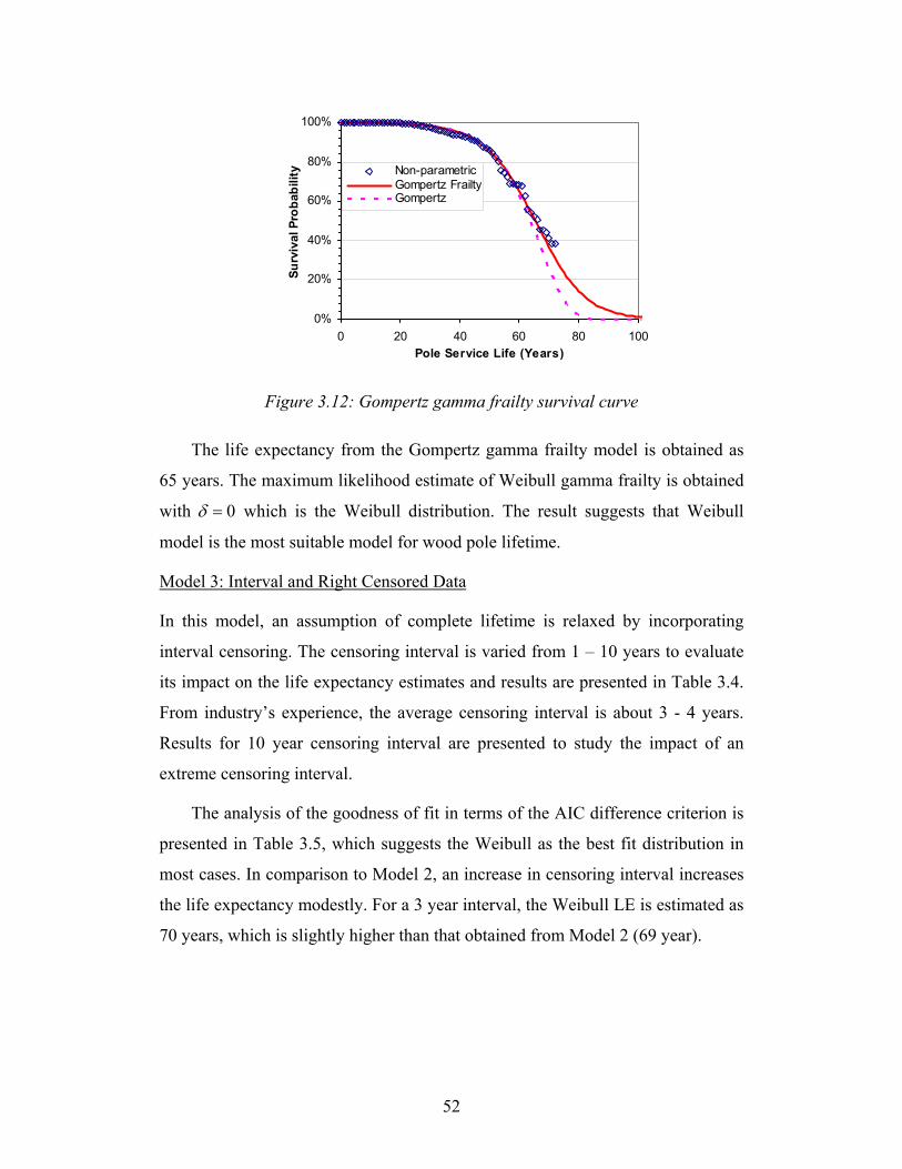
52

0%

20%

40%

60%

80%

100%

0 20 40 60 80 100Pole Service Life (Years)

Surv

ival

Pro

babi

lity Non-parametric

Gompertz FrailtyGompertz

Figure 3.12: Gompertz gamma frailty survival curve

The life expectancy from the Gompertz gamma frailty model is obtained as

65 years. The maximum likelihood estimate of Weibull gamma frailty is obtained

with 0=δ which is the Weibull distribution. The result suggests that Weibull

model is the most suitable model for wood pole lifetime.

Model 3: Interval and Right Censored Data

In this model, an assumption of complete lifetime is relaxed by incorporating

interval censoring. The censoring interval is varied from 1 – 10 years to evaluate

its impact on the life expectancy estimates and results are presented in Table 3.4.

From industry’s experience, the average censoring interval is about 3 - 4 years.

Results for 10 year censoring interval are presented to study the impact of an

extreme censoring interval.

The analysis of the goodness of fit in terms of the AIC difference criterion is

presented in Table 3.5, which suggests the Weibull as the best fit distribution in

most cases. In comparison to Model 2, an increase in censoring interval increases

the life expectancy modestly. For a 3 year interval, the Weibull LE is estimated as

70 years, which is slightly higher than that obtained from Model 2 (69 year).

53

Table 3.5: Pole life expectancy and lifetime distribution data – Model 3

DistributionCensoring

Interval (years)

Life Expectancy

(years)

Standard Deviation C.O.V (%)

Weibull β α1 4.48 73.67 67.21 16.75 252 4.18 76.19 69.23 18.41 273 4.05 77.47 70.26 19.25 274 3.92 78.76 71.31 20.11 285 3.81 80.08 72.38 20.98 2910 3.33 87.03 78.10 25.64 33

Gompertz B C1 0.0001 1.1109 61.25 14.35 232 0.0001 1.1073 61.71 14.67 243 0.0001 1.1039 62.17 14.99 244 0.0001 1.1008 62.64 15.30 245 0.0001 1.0979 63.10 15.62 2510 0.0002 1.0853 65.48 17.19 26

Log-Logistic β α1 4.49 72.31 78.55 35.34 452 4.35 73.42 80.23 37.66 473 4.21 74.55 81.95 40.09 494 4.08 75.70 83.74 42.64 515 3.96 76.88 85.58 45.33 5310 3.46 83.15 95.79 61.44 64

Parameters

Table 3.6: AIC differences among parametric models

Censoring Interval (years)

Weibull Gompertz Log-logistic

1 0 450 902 0 526 663 0 592 464 0 648 305 0 700 1810 24 880 0

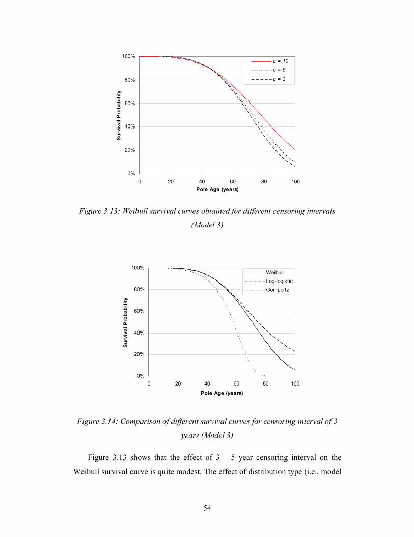
54

0%

20%

40%

60%

80%

100%

0 20 40 60 80 100Pole Age (years)

Sur

viva

l Pro

babi

lity

c = 10

c = 5

c = 3

Figure 3.13: Weibull survival curves obtained for different censoring intervals

(Model 3)

0%

20%

40%

60%

80%

100%

0 20 40 60 80 100

Pole Age (years)

Sur

viva

l Pro

babi

lity

WeibullLog-logisticGompertz

Figure 3.14: Comparison of different survival curves for censoring interval of 3

years (Model 3)

Figure 3.13 shows that the effect of 3 – 5 year censoring interval on the

Weibull survival curve is quite modest. The effect of distribution type (i.e., model

55

uncertainty) on survival curve is illustrated in Figure 3.14 (c= 3 year). The tail of

the survival curve is quite sensitive to the distribution type. The log-logistic

distribution leads to an upper bound life expectancy of 82 years, whereas the

Gompertz model provides a lower bound of 62 years. The reason is that the

hazard rate in the Gompertz model increases with age much more rapidly than in

the other two models, which leads to a low value of life expectancy. Since the

survival curve is a key input to the life-cycle cost analysis, it is important to

evaluate the sensitivity of model uncertainty to the cost optimization problem.

This issue is discussed in Section 4.2.1.

3.4.1.3 Remarks: Model Comparison

Figure 3.15 illustrates the effect of the three modeling assumptions regarding the

inspections data on estimates of the Weibull survival curve. The analysis in

Model 1 is simplistic as it ignores a vast amount of information about the survival

of a large fraction of the sample. Model 1 is therefore the most pessimistic model,

and it provides an unrealistic lower bound estimate of pole life expectancy (LE

=40 years).

0%

20%

40%

60%

80%

100%

0 20 40 60 80 100

Pole Age (years)

Sur

viva

l Pro

babi

lity

Model 3

Model 2

Model 1

Figure 3.15: Comparison of the Weibull survival curves obtained from the three

inspection models

56

Model 2 improves significantly the estimates of survival probabilities by

consideration of the right censored data, and it leads to LE = 69 year. The survival

curve of Model 3 (c=3) is in a close agreement with Model 2, and estimated LE =

70 years. The analysis illustrates that the censoring interval of 3 - 5 years has

limited sensitivity to the life expectancy estimates. The reason for this

insensitivity is that the interval censored data is a very small fraction (5.46%) of

the sample. The effect of censoring interval on LE increases with increase in the

proportion of data in the sample.

3.4.2 Lifetime Distribution of Oil Circuit Breakers

3.4.2.1 Introduction

Oil circuit breakers (OCB) are used to switch circuits and equipment in and out of

a system in a substation as shown in Figure 3.16. They are oil filled to provide

cooling and to prevent arcing when the switch is activated. The oil circuit breaker

has number of sub-components like contacts, pushings, lifting rods etc. and all

these components has to perform well in order to the circuit breaker to work.

Figure 3.16: Oil Circuit Breaker

57

As the oil breaker is in usage the components are subjected to operating load

and environmental effects which trigger the deterioration process. Hence the oil

breakers have to be subjected to periodic maintenance to ensure its smooth

functioning. The maintenance packages vary from visual inspection conducted

every six months to the intrusive maintenance which is the most expensive and

conducted every 7 years.


The data discussed in this section is obtained from a power industry which has

collected maintenance data on oil circuit breaker (OCB) from 1999 to 2004. The

majority of the OCBs are 27.6 kV and 44kV which consist of 752 Oil breakers

that have undergone selective intrusive (SI) maintenance. For each OCB under

selective intrusive maintenance has 5-6 individual tasks to access the condition of

the oil-breaker and each is given a condition rating of CR1(good)-CR4(bad). SI

maintenance package consists of the tasks as shown in Table 3.7.

Table 3.7: Description of SI maintenance tasks

SI Task Description T2 Check insulation condition. T3 Inspect contacts and interrupters. T4 Measure resistance/resistors. T5 Contact wipe measurement (analyzer rod). T6 Inspect internal components and tank

Data on Task T1 is not provided and hence will not be discussed here. Each

task aims at specific degradation mechanism for various components of OCB. The

condition rating of an OCB in each task is ranked as shown in Table 3.8

Table 3.8: Description of condition rating in each task

Condition Rating

Description

CR1 Condition like new

CR2 Condition as expected (no unusual degradation, functional as per design)

CR3 Signs of degradation CR4 Poor condition

58

End of Life Criterion

An OCB with condition rating CR4 in a given maintenance category is assumed

to be at the end of life (incipient failure) with respect to that maintenance

category. A rating of CR3 means that remaining life is approximately 3 years. A

rating of CR1 or CR2 is considered as the OCB in a good functional state as per

design. The average SI maintenance interval is 7 years. Each task is assumed as

independent degradation mechanisms; hence the estimation of lifetime of each

degradation/task is essential for estimating the overall breaker lifetime. The

results on lifetime analysis on each task are discussed in next section.

3.4.2.3 Statistical Lifetime Analysis

SI inspection data under each task is grouped to conduct lifetime analysis. Most of

the breakers does not have record on the time of previous inspection and is thus

assumed the average inspection interval of 7 years. Weibull distribution model is

assumed to model the aging or deterioration effects in each task. The failure rate

is assumed to linearly increase with time (Rayleigh Model) based on the

preliminary analysis conducted on maintenance data. When the failure rate is

assumed as constant (Exponential Model) the model underestimates the

probability of failure, whereas when the failure rate is assumed highly nonlinear

the model may overestimate the probability of failure.

The breakers were assumed to be in condition CR1 at the outset of the

interval. The breaker with condition rating CR4 in a given maintenance category

is considered as complete observation. The breaker with condition rating CR3 in a

given maintenance category is considered as interval censored towards right of

the observation since it is assumed that the remaining life is approximately 3

years. The breaker with condition CR1 and CR2 are considered as right censored

observations. The estimation of lifetime distribution is conducted using maximum

likelihood method discussed in Section 3.3.4. The mean lifetimes for different

task categories is shown in the Table 3.9

59

Table 3.9: Mean lifetime of a breaker under different SI Inspection Tasks

Task T2 T3 T4 T5 T6

Number of OCBs inspected 708 709 278 696 699

Mean Lifetime, Years (Rayleigh) 39 13 21 15 19

Mean Lifetime, Years (Exponential) 547 40 81 43 104

The mean life time is the lowest (13 years) with respect to the conditions of

contacts and interrupters (T3). The mean lifetime is the highest (39 years) with

respect to the insulation condition. The condition of tank (T6) reaches to CR4 on

average in 19 years of service life. The mean lifetimes obtained from exponential

distribution are much higher which underestimates the probability of failure.

The lifetime distributions are shown in Figure 3.17 and 3.18. The area under

the distribution between 0 and 7 years shows the probability of a breaker reaching

CR4. For example, the probability of reaching CR4 in the task T3 (contacts and

interrupters) is approximately 20%, estimated from Figure 3.17.

0%

1%

2%

3%

4%

5%

6%

0 10 20 30 40 50 60

Time (Years)

Prob

abili

ty D

ensi

ty (P

DF)

T4

T3

7

T4

T3

Figure 3.17: Lifetime distribution with respect to the tasks T3 and T4

60

0%

1%

2%

3%

4%

5%

6%

0 10 20 30 40 50 60

Time (Years)

Prob

abili

ty D

ensi

ty (P

DF)

T5T6T2

7

T5

T6

T2

Figure 3.18: Lifetime distribution with respect to the tasks T2, T5 and T6

3.4.2.4 Maintenance Interval Optimization

The first step in optimizing a maintenance program is to increase the interval of SI

maintenance from 7 years to say 8 or 10 years. An increase in SI interval will also

increase the probability of the breaker reaching in CR4 condition. This will

increase the probability of functional failure of a breaker. The contacts and the

interrupters appear to be the most stressed parts of the breaker, since they have the

lowest mean service life. If the SI interval is increased from 7 to 8 years, a

maximum 5% increase in probability is estimated for the task T3 (contacts and

interrupters). In other cases, the increase in probability is less than 5%.

The probability of a breaker reaching in CR4 condition for different

inspection intervals is presented in the Table 3.10. The lifetime distributions given

in Figure 3.17 and 3.15 were used to derive these probability estimates.

61

Table 3.10: Probability of an OCB reaching in CR4 condition under different SI

task

Probability of Reaching in CR4 Condition

Task

Mean Lifetime of Breaker (years)

7 years (Current interval)

8 years 10 years

T2 39 2% 3% 5% T3 13 20% 25% 37% T4 21 8% 11% 16% T5 15 15% 19% 28% T6 19 10% 13% 19%

3.4.2.5 Remarks

The maintenance data collected on OCB gives very little information on

component lifetimes. This creates difficulty in estimating the lifetime distribution

of OCB. The time since previous inspection is taken as 7 years and the condition

in each task define the lifetime of OCB. Weibull distribution with shape

parameter 2 is assumed to model the lifetime in each task from aging effects.

Lifetime distributions in each task are estimated from maximum likelihood

method.

The probabilistic analysis of breaker inspection data enables the development

of risk-based models to optimize the maintenance program and minimize the

associated life-cycle costs. The service lifetime ends when a breaker enters in

CR4 (poor condition), since it triggers a corrective maintenance of the breaker. It

does not reflect the true probability of functional failure of the breaker. For the

sake of a proper risk assessment, a correlation between the CR4 rating and

breaker probability of failure must be investigated. The past records of breaker

failure should be examined to establish this correlation. There is a potential to

increase the inspection interval from 7 to 8 or 10 years for some of the SI tasks

that can result in cost savings.

62

3.4.3 Estimation of Lifetime Distribution of Electric Insulators


Electric insulators are an important component on power transmission lines for

electric utilities. Insulators experience degradation with usage and eventually fail.

Maintenance of such insulators is crucial in maintaining the network reliability of

power infrastructure. The lifetime of the insulators is required for maintenance

decisions. Probabilistic lifetime distribution for insulators can be estimated from

field failure data. The insulators are designed with high lifetime and so the

failures observed are very few.

A mockup inspection data on insulators obtained from the power utility for a

specific population is shown in Table 3.11. The data shown in Table 3.11 is not

considered in the analysis but reflects the actual data obtained from industry. The

data obtained actually gives information on current status of insulators at the time

of inspection. This is similar to the case of wood pole inspection but in this case

there is insufficient data on aging population.

Table 3.11: Inspection data of insulators tested by power utility

Age (ti) Number Defective

(di)

Number Tested (ni)

21 0 25 24 0 100 25 2 500 26 5 1000 27 5 1000 28 30 6000 29 12 2000 30 10 1500 31 6 1000 32 7 500

The lifetime or failure of the insulator is defined as the time to enter defective

state. The precise lifetime of the defective insulators is unknown, which happened

sometime between installation and inspection time. The age of the insulators at

63

the time of inspection are derived from their installation dates. Such type of data

is called left censored observations. This section discusses the problem of

estimating the insulator lifetime distribution from current status data.

3.4.3.2 Statistical Data Analysis

The data from actual inspection of insulators similar to that shown in Table 3.11

is considered for the analysis. The non-parametric estimates are first calculated by

Maximum Likelihood method as discussed in Section 3.3.3.4. The plot on the

survival probability estimates along with 95% confidence limits is shown in

Figure 3.19.

97.5%

98.0%

98.5%

99.0%

99.5%

100.0%

0 5 10 15 20 25 30 35Age (years)

Surv

ival

Pro

babi

lity

Upper 95%CL

MLE

Low er 95%CL

Figure 3.19: Non parametric MLE estimates of survival probabilities

The survival estimates of the insulators from Figure 3.19 are high indicating that

the insulators have very high lifetime. The survival probability estimate for

insulator age 32 years is 98.7% which is the oldest insulator in service. The

parameters of Weibull distribution are estimated as discussed in Section 3.3.4.1.

The maximum likelihood estimate in this case converged to a very high life

expectancy of 521 years and C.O.V of 61%. Although there exists a local

convergent solution with shape parameter as 5.27 and scale as 74.56 with life

expectancy of 69 years and C.O.V of 22%. The reason for this discrepancy can be

seen in Figure 3.20 where the MLE tries to fit observations collected in the early

insulator lifetime.

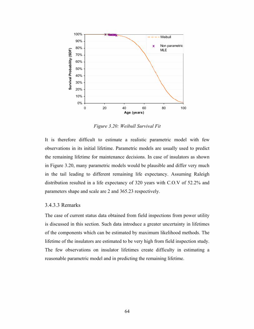
64

0%

10%

20%

30%

40%

50%

60%

70%

80%

90%

100%

0 20 40 60 80 100Age (years)

Surv

ival

Pro

babi

lity

(SD

F)

Weibull

Non parametricMLE

Figure 3.20: Weibull Survival Fit

It is therefore difficult to estimate a realistic parametric model with few

observations in its initial lifetime. Parametric models are usually used to predict

the remaining lifetime for maintenance decisions. In case of insulators as shown

in Figure 3.20, many parametric models would be plausible and differ very much

in the tail leading to different remaining life expectancy. Assuming Raleigh

distribution resulted in a life expectancy of 320 years with C.O.V of 52.2% and

parameters shape and scale are 2 and 365.23 respectively.

3.4.3.3 Remarks

The case of current status data obtained from field inspections from power utility

is discussed in this section. Such data introduce a greater uncertainty in lifetimes

of the components which can be estimated by maximum likelihood methods. The

lifetime of the insulators are estimated to be very high from field inspection study.

The few observations on insulator lifetimes create difficulty in estimating a

reasonable parametric model and in predicting the remaining lifetime.

65

3.4.4 Analysis of Feeder Pipe Cracking


The case study is from the inspection of 380 feeder pipes from a nuclear reactor.

Feeder pipes are one of the critical components of primary heat transport system

in nuclear reactor. The data consists of the time to crack detection of eight feeder

pipes and time of last inspection for three of them. Out of the 8 feeder pipe cracks

three are through wall cracks resulting in pipe leakage. Crack depth measurements

on the 8 observations are used to estimate the growth rate (crack depth/detection

time). Since the feeder pipes are not continuously monitored the growth of crack

is assumed to follow linear growth model. The rest 372 pipes are still in service

and have not shown any cracks.

Lifetime distribution model based on three leak observations and the rest 377

right censored observations is analyzed. Method of maximum likelihood

assuming Weibull distribution resulted in life expectancy of 43 years and variance

of lifetime as 95. The uncertainty in estimating the life expectancy is high due to

sparse data on feeder lifetimes as shown in Table 3.12.

Table 3.12: Parameters of Weibull lifetime distribution

Model Parameters Estimate Lower 95% CL

Upper 95% CL

Shape (β) 5.06 1.65 15.54 Scale (α) 47.06 15.82 139.98

Weibull Mean Lifetime ( Tμ ) 43.24 15.58 120.04

This lifetime model ignores the fact that five feeder pipes having partial

cracks. The problem can also be analyzed by modeling the crack growth rate. The

problem is to estimate the lifetime distribution of pipe failure and annual

probability of leak prediction in future time interval is discussed in the next

section.

66

3.4.4.2 Statistical lifetime Model

One way to analyze the data is by estimating the uncertainty in crack growth rate

by modelling the crack growth rate observations by Weibull distribution. The

probability that a pipe with thickness h and with growth rate r fails at time t is

given as )Pr( hrt ≥× , when growth rate follows a Weibull distribution with

parameters (α, β)

⎟⎟⎠

⎞⎜⎜⎝

⎛⎟⎠⎞

⎜⎝⎛ ×−=⎟

⎠⎞

⎜⎝⎛ ≥

β

α1expPr

th

thr (3.50)

0exp)( >⎟⎟⎠

⎞⎜⎜⎝

⎛⎟⎠⎞

⎜⎝⎛−= t

thtF

β

α (3.51)

This shows that the derived distribution of t follows Inverse Weibull with

parameters (h/α, β). The first moment or mean lifetime of the inverse Weibull is

given as

⎟⎟⎠

⎞⎜⎜⎝

⎛−Γ×⎟

⎠⎞

⎜⎝⎛=

βαμ 11h

t (3.52)

The observations on growth rate are analysed by method of maximum

likelihood to fit a Weibull distribution.

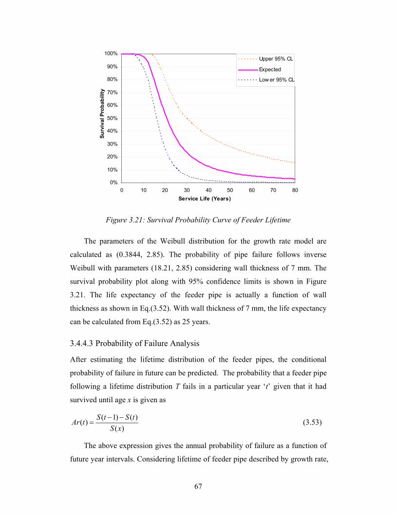
67

0%

10%

20%

30%

40%

50%

60%

70%

80%

90%

100%

0 10 20 30 40 50 60 70 80Service Life (Years)

Surv

ival

Pro

babi

lity

Upper 95% CL

Expected

Low er 95% CL

Figure 3.21: Survival Probability Curve of Feeder Lifetime

The parameters of the Weibull distribution for the growth rate model are

calculated as (0.3844, 2.85). The probability of pipe failure follows inverse

Weibull with parameters (18.21, 2.85) considering wall thickness of 7 mm. The

survival probability plot along with 95% confidence limits is shown in Figure

3.21. The life expectancy of the feeder pipe is actually a function of wall

thickness as shown in Eq.(3.52). With wall thickness of 7 mm, the life expectancy

can be calculated from Eq.(3.52) as 25 years.

3.4.4.3 Probability of Failure Analysis

After estimating the lifetime distribution of the feeder pipes, the conditional

probability of failure in future can be predicted. The probability that a feeder pipe

following a lifetime distribution T fails in a particular year ‘t’ given that it had

survived until age x is given as

)()()1()(

xStStStAr −−

= (3.53)

The above expression gives the annual probability of failure as a function of

future year intervals. Considering lifetime of feeder pipe described by growth rate,

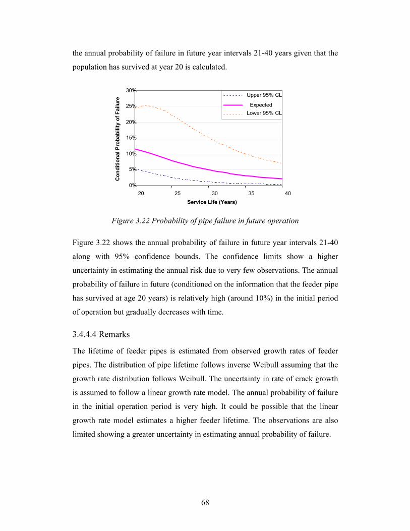
68

the annual probability of failure in future year intervals 21-40 years given that the

population has survived at year 20 is calculated.

0%

5%

10%

15%

20%

25%

30%

20 25 30 35 40 Service Life (Years)

Con

ditio

nal P

roba

bilit

y of

Fai

lure

Upper 95% CL Expected

Lower 95% CL

Figure 3.22 Probability of pipe failure in future operation

Figure 3.22 shows the annual probability of failure in future year intervals 21-40

along with 95% confidence bounds. The confidence limits show a higher

uncertainty in estimating the annual risk due to very few observations. The annual

probability of failure in future (conditioned on the information that the feeder pipe

has survived at age 20 years) is relatively high (around 10%) in the initial period

of operation but gradually decreases with time.

3.4.4.4 Remarks

The lifetime of feeder pipes is estimated from observed growth rates of feeder

pipes. The distribution of pipe lifetime follows inverse Weibull assuming that the

growth rate distribution follows Weibull. The uncertainty in rate of crack growth

is assumed to follow a linear growth rate model. The annual probability of failure

in the initial operation period is very high. It could be possible that the linear

growth rate model estimates a higher feeder lifetime. The observations are also

limited showing a greater uncertainty in estimating annual probability of failure.

69

3.5 Conclusions

It is not always possible to observe complete lifetimes through periodic

inspections. In most cases, the observed lifetimes are either right-censored or

interval-censored. The chapter presents statistical methods to analyze various

types of incomplete data encountered from inspection of components in the

energy industry. The effect of incomplete lifetime data in estimating the lifetime

distributions is illustrated.

A comprehensive statistical analysis of realistic inspection data for estimating

the lifetime distribution of wood pole distribution networks is discussed. The

analysis concludes that the pole inspection data commonly collected by power

utilities should be modeled as a combination of interval-censored and the right-

censored sample of lifetimes. The analysis suggests that the pole survival curve is

well approximated with the Weibull probability distribution, and from the data

considered, the pole life expectancy is estimated at 69 years. The fitted

distribution and life expectancy estimate are data dependent, although the

methodology presented is general. A simplistic data analysis that ignores the

censoring of lifetime can result in a severe underestimation of life expectancy.

In the case of oil circuit breakers, there is insufficient data to quantify the

degradation. This is similar to the wood pole problem, in which the collecting of

inspection data has lately started in the service of OCB and there is insufficient

data to model the degradation by stochastic models. Lifetime models are therefore

used in estimating the lifetime distribution, using condition data from selective

intrusive inspections. The condition information on each task can be interpreted as

censored and complete lifetimes. The lifetimes are assumed to follow Weibull

distribution with linear failure rate (i.e shape parameter is fixed at 2) based on the

preliminary assessment of maintenance data. The lifetime distribution in each task

is estimated by the method of maximum likelihood. The estimated lifetime

distributions suggest that there is a potential to increase the inspection interval

from 7 years to 8 or 10 years, to achieve cost savings.

70

In case of electric insulators, the data obtained from power utilities is a

snapshot of the state of insulators from a single inspection. The exact lifetimes of

insulators are unknown, so the data type is therefore considered as current status.

From the available data, the survival probability estimates of insulators are

calculated to be very high. It is therefore difficult to estimate a realistic parametric

model since the remaining lifetime of the current population is uncertain.

The feeder cracking problem is another case in which there are only three

complete observations (leaks), and the rest as right censored. The life expectancy

in such a case can be estimated as 43 years, but there is greater uncertainty in the

estimate. The crack growth rate is of interest to engineers in feeder pipe life cycle

management. The probability of failure due to through-wall leakage is of concern.

The randomness in crack growth rate is used to derive the distribution of feeder

lifetime. The lifetime distribution is derived as inverse Weibull, while the crack

growth rate is assumed to follow Weibull distribution. The life expectancy is

estimated to be 25 years, a value which keeps the current age of feeder pipe near

life expectancy, leading to a higher annual probability of pipe failure after another

five years.

The major contribution of the lifetime distribution chapter is to present the

methodology for estimating realistic lifetime distribution from incomplete lifetime

data usually obtained from field inspection studies in energy infrastructure. The

chapter also discusses the difficulty in interpreting and estimating the lifetime

distribution from highly censored observations.

71

CHAPTER 4 LCM MODEL USING LIFETIME DISTRIBUTIONS

4.1 Overview

This Chapter discusses the application of probabilistic models in equipment life

cycle management. Firstly the age based replacement policy popular in energy

industry is applied for wood pole management. The sequential inspection based

component replacement models for a distributed population are illustrated. The

effect of imperfect preventive maintenance on maintenance decisions is modeled

using the concept of virtual age.

4.2 Age Based Replacement Policy

The age-based replacement policy is the conceptually simplest and an effective

policy to implement in a system with large population of relatively inexpensive

components (Barlow and Proschan, 1965). In this policy, a component is replaced

at the age t0 or at failure, whichever occurs first. The objective of the policy is to

select the replacement age to that minimizes the life-cycle cost rate associated

with the policy.

Consider the cost of preventive replacement as CP, which includes the

inspection, labour and equipment costs. An additional cost incurred due to failure

is denoted as CF, which includes additional costs due to power interruption and

corrective repair to be done under an emergency.

According to the renewal theorem, the replacement age (to) should be

selected to optimize the expected average cost rate, Z(t0), in a long run (Barlow

and Proschan, 1965). The expected cost rate is defined as the ratio of the expected

cycle cost to the expected cycle length:

)][)]([)( 0

L

o

TEtCEtZ = (4.1)

72

where C(to) is the life-cycle cost and TL is the cycle length, defined as the time

between replacements. It is a random variable that is related to the life time

distribution and replacement age with cumulative distribution given as

)()(

1

)()(

o

oTT tx

txxFxF

L ><

⎟⎟⎠

⎞= (4.2)

The expected cycle length is obtained as

∫∫ =−=∞ o

L

t

TTL dxxSdxxFTE00

)())(1(][ (4.3)

The expected cost is derived as E[C(to)] = )( oTFP tFCC + . Finally, the

expected cost rate is obtained as

∫

+=

0

0

00

)(

)()( t

T

FP

dxxS

tFCCtZ (4.4)

The optimum replacement time is determined by minimizing Z(to) with

respect to to as

0)(

0

0 =dt

tdZ (4.5)

which can be simplified to

F

Pt

TT CC

dxxSthtS +=+ ∫ 1)()()(0

000 (4.6)

where h(to) is hazard rate at the replacement age. The optimum replacement age is

the solution of Eq.(4.6) in terms of the cost ratio, CP/CF, and the survival function.

4.2.1 Wood Pole Replacement Problem

Figure 4.1 presents a generic plot of the optimal replacement age (topt) versus the

cost ratio is obtained by numerically solving Eq.(4.6) and using the best-fit

Weibull distribution derived for the three models discussed in Section 3.4.1.

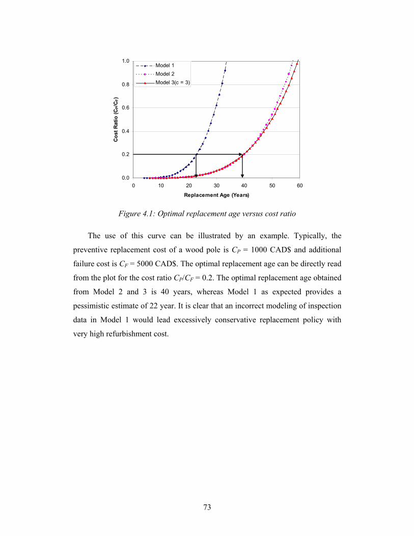
73

0.0

0.2

0.4

0.6

0.8

1.0

0 10 20 30 40 50 60

Replacement Age (Years)

Cos

t Rat

io (C

P/C F

)

Model 1Model 2Model 3(c = 3)

Figure 4.1: Optimal replacement age versus cost ratio

The use of this curve can be illustrated by an example. Typically, the

preventive replacement cost of a wood pole is CP = 1000 CAD$ and additional

failure cost is CF = 5000 CAD$. The optimal replacement age can be directly read

from the plot for the cost ratio CP/CF = 0.2. The optimal replacement age obtained

from Model 2 and 3 is 40 years, whereas Model 1 as expected provides a

pessimistic estimate of 22 year. It is clear that an incorrect modeling of inspection

data in Model 1 would lead excessively conservative replacement policy with

very high refurbishment cost.

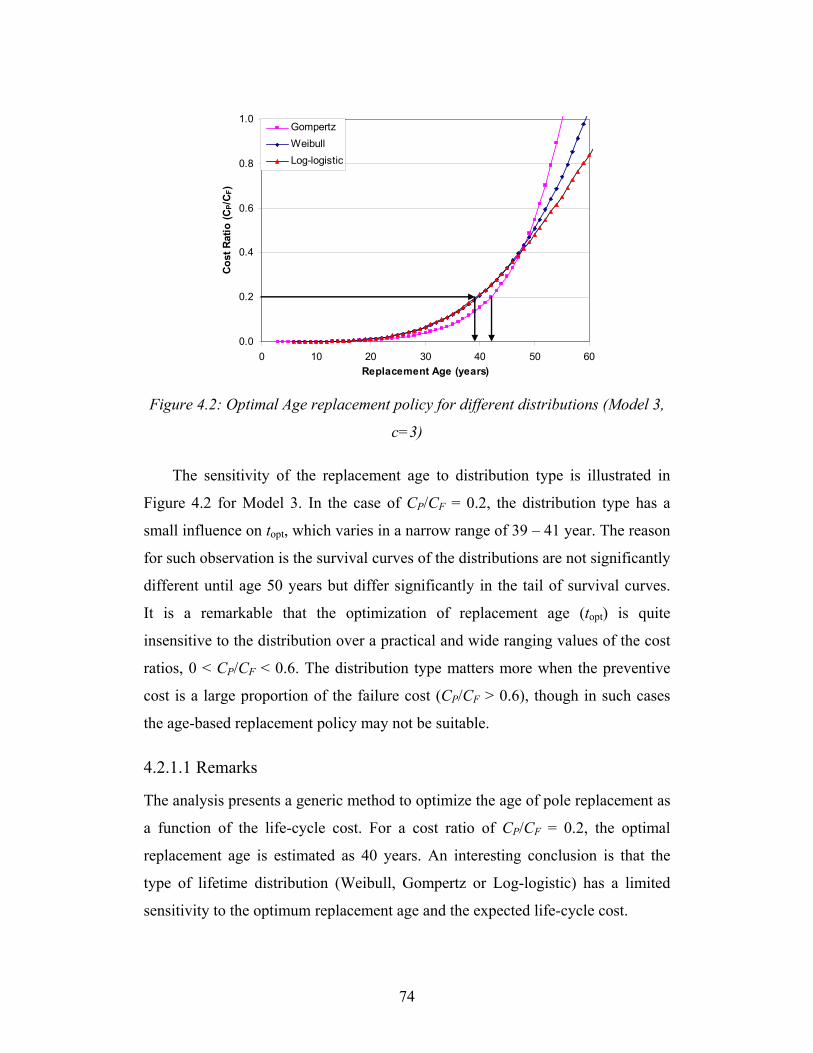
74

0.0

0.2

0.4

0.6

0.8

1.0

0 10 20 30 40 50 60Replacement Age (years)

Cos

t Rat

io (C

P/C F

)

GompertzWeibullLog-logistic

Figure 4.2: Optimal Age replacement policy for different distributions (Model 3,

c=3)

The sensitivity of the replacement age to distribution type is illustrated in

Figure 4.2 for Model 3. In the case of CP/CF = 0.2, the distribution type has a

small influence on topt, which varies in a narrow range of 39 – 41 year. The reason

for such observation is the survival curves of the distributions are not significantly

different until age 50 years but differ significantly in the tail of survival curves.

It is a remarkable that the optimization of replacement age (topt) is quite

insensitive to the distribution over a practical and wide ranging values of the cost

ratios, 0 < CP/CF < 0.6. The distribution type matters more when the preventive

cost is a large proportion of the failure cost (CP/CF > 0.6), though in such cases

the age-based replacement policy may not be suitable.

4.2.1.1 Remarks

The analysis presents a generic method to optimize the age of pole replacement as

a function of the life-cycle cost. For a cost ratio of CP/CF = 0.2, the optimal

replacement age is estimated as 40 years. An interesting conclusion is that the

type of lifetime distribution (Weibull, Gompertz or Log-logistic) has a limited

sensitivity to the optimum replacement age and the expected life-cycle cost.

75

4.3 Sequential Inspection Based Replacement Model

4.3.1 Introduction

This section presents a risk based approach to manage components from a large

distribution networks. Network components being large in number play a

significant role in the overall Asset Management of the network system.

Maintenance of such a large infrastructure is a major problem that the asset

managers face in this competitive world. The population is so large that all

components cannot be inspected in any one year due to a prohibitively high

inspection cost and labour requirements. Therefore, there is need for the

development of quantitative methods on decisions related to inspection and

replacement strategies adopted by most network organizations.

The development of a probabilistic model for sequential inspection based

maintenance program is addressed in this section. The impact of replacement

strategies on life-cycle performance (i.e., risk and cost) is quantified. This

analysis can then be used to optimize the maintenance interval and replacement

rate in order to meet a performance target defined in terms the cost, risk or both

cost and risk.

In summary, this section presents a complete probabilistic risk-based

framework for life-cycle management of distribution networks. The approach has

a significant potential in minimizing the maintenance cost and risk and improving

asset management practices in general. The proposed model is generic, and is

equally applicable to the asset management of large infrastructures.

4.3.2 Estimation of Substandard Component Population

A probabilistic method is presented to estimate the fraction of substandard

components in the distribution network based on current component

demographics and survival curve estimated from the inspection data.

The model predicts the component “failure rate”, which is the annual rate of

components reaching the end of life in a specified year. The proportion of

76

substandard components in the distribution network is also estimated, which

directly relates to risk of failure or vulnerability associated with the integrity of

components in the network. The proportion of substandard components is

essential to the assessment of life-cycle cost and reliability analysis. The proposed

model will be applied to optimize component replacement strategies in the next

section.

4.3.2.1 Model

The age-specific failure associated with a component of age X years in a future

interval of t to t+1 year is estimated from the component survival curve, S(t), as a

conditional probability given as

( ) ⎟⎟⎠

⎞⎜⎜⎝

⎛ ++−+==≥+<≤

)()1()(

)(|1PrXS

tXStXStMXTtTt X (4.7)

An alternate expression for the conditional failure probability is given as

( ))(.)(

)()( tXhXS

tXStM X +⎟⎟⎠

⎞⎜⎜⎝

⎛ += (4.8)

where the first term in the bracket is the probability of an age X component

surviving up to age X+t, and the second term, h(X+t), is the hazard rate at age

X+t. The conditional failure probability in effect can be derived from the

conditional life-time distribution given as

⎟⎟⎠

⎞⎜⎜⎝

⎛ +=

)()()(

XStXftM T

X (4.9)

where )(xfT denotes the component life-time density function.

A similar approach as shown in Eq. (4.7) is discussed by Li, et al., (2004) to

predict the number of failures in a planning horizon. Since the population consists

of components of different ages, as described by the age distribution, )(xf A , the

overall population failure rate in a future time interval t - t+1 year is obtained as

∑=

×=T

XAXP XftMtM

0

)()()( (4.10)

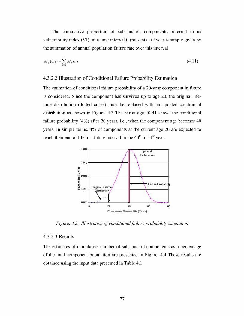
77

The cumulative proportion of substandard components, referred to as

vulnerability index (VI), in a time interval 0 (present) to t year is simply given by

the summation of annual population failure rate over this interval

∑=

=t

uPC uMtM

0

)(),0( (4.11)

4.3.2.2 Illustration of Conditional Failure Probability Estimation

The estimation of conditional failure probability of a 20-year component in future

is considered. Since the component has survived up to age 20, the original life-

time distribution (dotted curve) must be replaced with an updated conditional

distribution as shown in Figure. 4.3 The bar at age 40-41 shows the conditional

failure probability (4%) after 20 years, i.e., when the component age becomes 40

years. In simple terms, 4% of components at the current age 20 are expected to

reach their end of life in a future interval in the 40th to 41st year.

Figure. 4.3. Illustration of conditional failure probability estimation

4.3.2.3 Results

The estimates of cumulative number of substandard components as a percentage

of the total component population are presented in Figure. 4.4 These results are

obtained using the input data presented in Table 4.1

78

Table 4.1. Statistical input data for illustrative results

Item Average (years)

Standard Deviation (years)

Distribution Type

Age Distribution 30 15 Weibull

Lifetime Distribution 40 10 Weibull

Figure. 4.4 show the substandard components in the population that are

obtained from statistics from Table 4.1. The plot highlights the impact of

component demographics on the number of substandard components in absence

of an inspection and replacement program. For example, Figure. 4.4 show the

total (cumulative) number of substandard components after 20 years is estimated

as 70% on the basis of a component life expectancy of 40 years.

This analysis confirms the need for an effective inspection and replacement

program to limit the number of substandard components to an acceptable level.

0%

20%

40%

60%

80%

100%

0 5 10 15 20 25 30

Future Time (Years)

Subs

tand

ard

com

pone

nts

in

Popu

latio

n

Figure. 4.4. Future projection of substandard components in the population

79

0%

1%

2%

3%

4%

5%

6%

1 5 9 13 17 21 25 29

Forecast Year

Ann

ual F

ailu

re R

ate

Figure. 4.5. Annual failure rate in component population

The analysis model can be used to provide further insight into component

aging and failure rate. Considering the life expectancy as 40 years, the annual

conditional failure rates are projected in Figure. 4.5 In early years, the conditional

failure rate ranges from 3%-6%, but it declines rapidly after 20 years. The decline

is due to the fact that most aged components have already vanished from the

population leaving behind a much smaller cohort of relatively young components.

In this analysis, component replacement is not considered. The analysis with

component replacement is discussed in Section 4.4 using renewal theory.

4.3.2.4 Summary

A probabilistic model is presented for the estimation of the fraction of

substandard components as well as the annual conditional failure rate.

From the point of view of the risk of line failure, the cumulative (total)

number of substandard components is relevant. The conditional failure rate on the

other hand plays a role in the estimation of replacement rate, as shown in the next

section.

The number of substandard component is projected, which underscore the

need for an effective component replacement program. Otherwise, the

substandard component population would become so large that it would reduce

80

distribution network reliability and overwhelm maintenance activities in the

future.

4.3.3 Probabilistic Asset Management Model

To maintain reliability of the distribution system network, an effective program

for the replacement of substandard components is necessary. The replacement

program has two main elements, namely the inspection interval and the

component replacement rate.

The section presents a probabilistic model to quantify the impact of the

inspection interval and the annual component replacement rate, and relates these

to limiting the risk that the substandard components in the population may pose to

the system. A sequential inspection based replacement strategy is discussed in this

section. This analysis is essential to support the life-cycle cost estimation model

presented in the next section.

4.3.3.1 Model for Sequential Inspection and Replacement Program

This section presents a conceptual model of the sequential inspection and

replacement program. A sequential program means that only a part of the

component population is inspected in a given year, such that it takes T years to

complete the inspection of the entire population. It is in contrast with maintenance

strategies used in other industries (e.g., aerospace and chemical), in which an

entire component population is inspected in a given year of inspection.

To illustrate the concept of the sequential program, consider the case of a 5-

year inspection cycle as shown in Figure 4.6. To begin with (year 0), the

distribution component population is basically divided into 5 blocks, and one

block will be sequentially inspected each year. Substandard components found

during an inspection will be replaced by new components (age 0). It means that

component replacement takes place in the population block under inspection only.

81

In year 1, block-1 is inspected and due to component replacement, the

average component age is reduced and its age distribution is modified. Population

blocks 2-5 are unattended.

In year 2, block-2 is subject to inspection and replacement, and blocks 1, 3-5

are unattended. The substandard components continue to accumulate in blocks 3-

5.

In year 3, block-3 is subject to inspection and replacement work. Components

in block 4-5 are not inspected so far. Furthermore, previously inspected blocks 1-

2 experience progressive aging as well. However, the conditional failure rate in

previously inspected blocks is expected to be smaller than that in non-inspected

blocks. The difference between the two depends on the replacement rate during

the inspection.

The process continues as shown in Figure 4.6, and all the blocks are

inspected at the end of year 5. However, substandard components are not

completely eliminated from the population due to progressive component aging in

previously inspected blocks 1-4.

The inspection cycle continues to be repeated over the forecast period,

typically 30 years.

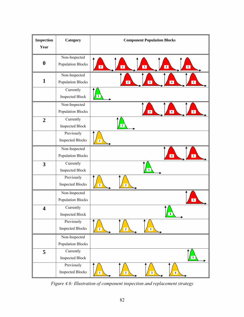
82

Inspection

Year

Category Component Population Blocks

0 Non-Inspected

Population Blocks 1 2 3 4 5

1 Non-Inspected

Population Blocks 2 3 4 5

Currently

Inspected Block 1

Non-Inspected

Population Blocks 3 4 5

2 Currently

Inspected Block 2

Previously

Inspected Blocks 1

Non-Inspected

Population Blocks 4 5

3 Currently

Inspected Block 3

Previously

Inspected Blocks 1

2

Non-Inspected

Population Blocks 5

4 Currently

Inspected Block 4

Previously

Inspected Blocks 1

2

3

Non-Inspected

Population Blocks

5 Currently

Inspected Block 5

Previously

Inspected Blocks 1

2

3

4

Figure 4.6: Illustration of component inspection and replacement strategy

83

4.3.3.2 Computation

In a distribution network, consider that the total number of components to be

managed is M. It is planned to inspect these components over an T year inspection

interval, so that the component population is divided into T blocks. The number of

components in each block is N = M/T. The component sample size for annual

inspection is NI = N. The component replacement is carried out based on their

condition. The blocks are inspected sequentially, and it takes T years to inspect

the population completely. Considering a forecast period of TF (= 30 years), the

number of inspection cycles = TF /T.

The probabilistic analysis model is developed to estimate:

(1) The number of remaining substandard components in the component

population for a chosen inspection interval (T years). It is a proxy measure of

residual risk or vulnerability to failure in the distribution network.

(2) The component replacement rate in any given year, which is needed to

compute the cost of component replacement.

The proportion of components of age Xk in kth block turning into substandard

state in an interval t1 – t2 years is defined as

)()(

)()(),,( 21

21 kAk

kkkS Xf

XStXStXS

ttXP ×⎟⎟⎠

⎞⎜⎜⎝

⎛ +−+= (4.12)

where fA(Xk) denotes the component age distribution at the time of reference t in a

component block. Recall that S(t) is the survival probability.

The fraction (%) of substandard components in a kth block is given as

∑=

=100

12121 ),,(),,(

XkSS ttXPttkD (4.13)

The total number of substandard components in the entire population is the

sum of rates of substandard components over T blocks:

∑=

=T

kSS ttkDNttN

12121 ),,(),( (4.14)

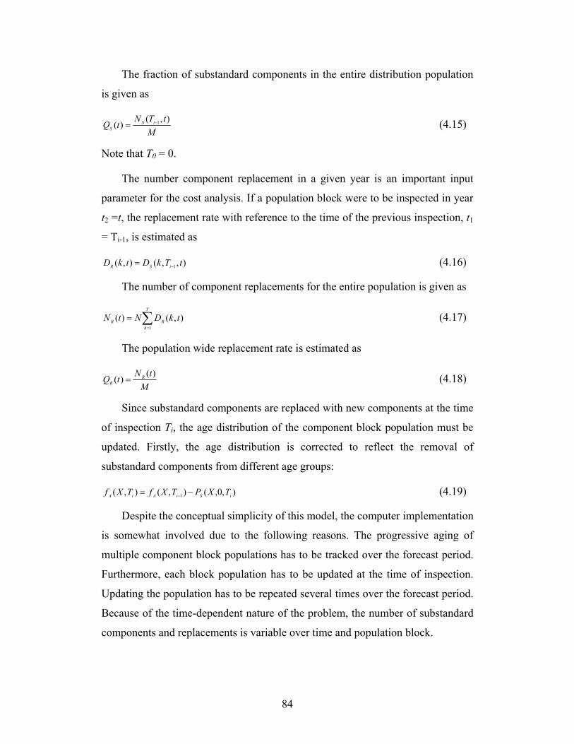
84

The fraction of substandard components in the entire distribution population

is given as

MtTNtQ iS

S

),()( 1−= (4.15)

Note that T0 = 0.

The number component replacement in a given year is an important input

parameter for the cost analysis. If a population block were to be inspected in year

t2 =t, the replacement rate with reference to the time of the previous inspection, t1

= Ti-1, is estimated as

),,(),( 1 tTkDtkD iSR −= (4.16)

The number of component replacements for the entire population is given as

∑=

=T

kRR tkDNtN

1

),()( (4.17)

The population wide replacement rate is estimated as

MtNtQ R

R

)()( = (4.18)

Since substandard components are replaced with new components at the time

of inspection Ti, the age distribution of the component block population must be

updated. Firstly, the age distribution is corrected to reflect the removal of

substandard components from different age groups:

),0,(),(),( 1 iSiAiA TXPTXfTXf −= − (4.19)

Despite the conceptual simplicity of this model, the computer implementation

is somewhat involved due to the following reasons. The progressive aging of

multiple component block populations has to be tracked over the forecast period.

Furthermore, each block population has to be updated at the time of inspection.

Updating the population has to be repeated several times over the forecast period.

Because of the time-dependent nature of the problem, the number of substandard

components and replacements is variable over time and population block.

85

4.3.3.3 Replacement Strategy

In this strategy, only those components are replaced that are determined to be in

substandard condition through inspection. This approach is economically

beneficial because unnecessary component replacements are avoided. However,

this approach has a drawback in case of a long inspection interval combined with

an aged component population. The drawback is that it replaces substandard

components that are present in the population only, but ignores components that

have potential to reach end of life during the inspection interval. In summary, this

strategy may not be effective when the inspection interval is long.

4.3.3.4 Results

4.3.3.4.1 General

The section illustrates the effect of the inspection interval (cycle length) affects on

the remaining number of substandard components, an indicator of risk, and the

replacement rate, a measure of cost of replacement program.

Table 4.2 describes three scenarios of the inspection program. The results are

obtained corresponding to the component life expectancy of 40 years.

Table 4.2. Inspection interval date for component replacement program

No Forecast Duration (TF years)

Inspection Interval (T

year)

Inspection Cycles (TF/T)

Inspection Sample (%of

population/year) (100/T%)

1 30 5 6 20% 2 30 15 2 6.67% 3 30 25 1 4%

4.3.3.4.2 Estimation of Remaining Substandard Poles

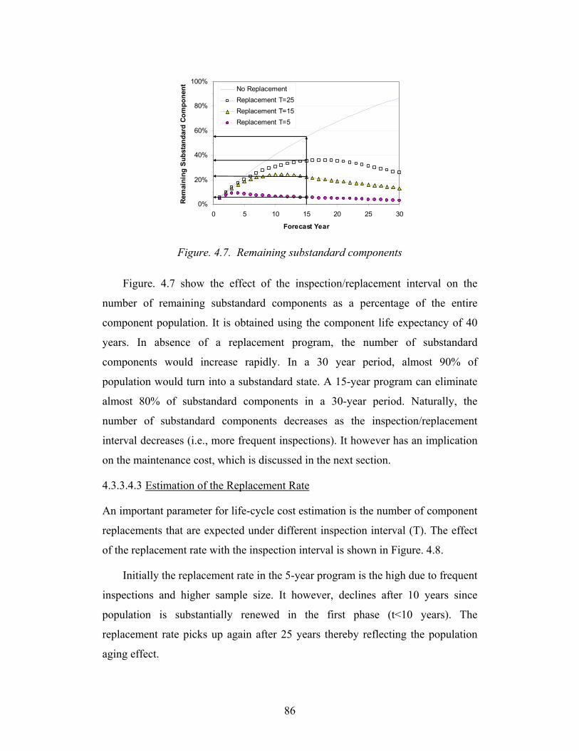
86

0%

20%

40%

60%

80%

100%

0 5 10 15 20 25 30

Forecast Year

Rem

aini

ng S

ubst

anda

rd C

ompo

nent No Replacement

Replacement T=25Replacement T=15Replacement T=5

Figure. 4.7. Remaining substandard components

Figure. 4.7 show the effect of the inspection/replacement interval on the

number of remaining substandard components as a percentage of the entire

component population. It is obtained using the component life expectancy of 40

years. In absence of a replacement program, the number of substandard

components would increase rapidly. In a 30 year period, almost 90% of

population would turn into a substandard state. A 15-year program can eliminate

almost 80% of substandard components in a 30-year period. Naturally, the

number of substandard components decreases as the inspection/replacement

interval decreases (i.e., more frequent inspections). It however has an implication

on the maintenance cost, which is discussed in the next section.

4.3.3.4.3 Estimation of the Replacement Rate

An important parameter for life-cycle cost estimation is the number of component

replacements that are expected under different inspection interval (T). The effect

of the replacement rate with the inspection interval is shown in Figure. 4.8.

Initially the replacement rate in the 5-year program is the high due to frequent

inspections and higher sample size. It however, declines after 10 years since

population is substantially renewed in the first phase (t<10 years). The

replacement rate picks up again after 25 years thereby reflecting the population

aging effect.

87

0%

2%

4%

6%

8%

0 5 10 15 20 25 30

Forecast Year

Repl

acem

ent R

ate

(%/y

ear)

T=5T=15T=25

Figure. 4.8. Estimation of component replacement rate

In the 15 year program, the replacement rate continuously increases in the fist

cycle (t ≤15 year) and reaches the peak value of 3.5%. In the second phase,

however, the replacement rate levels off at about 2%/year value.

4.3.3.4.4 Summary

The section presents a probabilistic model for the sequential inspection based

component replacement program. The model provides estimates of the remaining

number of substandard components, an indicator of risk, and the replacement rate,

a measure of the cost of the replacement program. The model illustrates the effect

of inspection interval and component life expectancy on these two parameters.

The model is the basis for life-cycle risk and cost analysis presented in the next

section.

4.3.4 Life-Cycle Risk and Cost Estimation

The section presents a model for estimating the life-cycle risk and costs associated

with the management of the distribution component asset. This model would

allow the optimization of the replacement program for minimizing the cost and

achieving a target reliability level.

88

4.3.4.1 Life-Cycle Risk

The substandard components are more vulnerable to failure under adverse

weather conditions or an accidental overload. Therefore, as the number of

substandard components increases in the distribution network, the risk of

unexpected component failure also increases with it. In other words, the risk of

component failure interrupting the electricity supply to customers is directly

proportional to the number of substandard components in the population, which

can be estimated from the model presented in this section.

The actual probability of failure of a substandard component is rather

difficult to estimate. Nevertheless, an average probability of failure can be

roughly estimated from the currently available component failure data.

Considering that approximately 250 component failures per year are currently

attributed to substandard component, and that there are approximately 6%

substandard components in 1.5 million distribution component population. The

probability of failure is therefore estimated as PF = 250/(0.06 ×1.5 ×106) =

2.77×10-3 ≈ 3×10-3 /substandard component/year. This estimate can be refined by

a formal statistical analysis of historical component failure data and conducting a

reliability analysis of component structure.

Conceptually, the annual rate of component failure in a forecast year t is

estimated as

FSF PtQtQ ×= )()( (4.20)

where QS(t) is the total fraction of substandard components in the distribution

population as given by Eq.(4.15).

The economic cost of a component failure (CF $/component) includes the

cost of emergency component replacement as well as the cost of supply

interruption. The annual risk associated with an aging network is estimated as

)()( tQCtR FFF = (4.21)

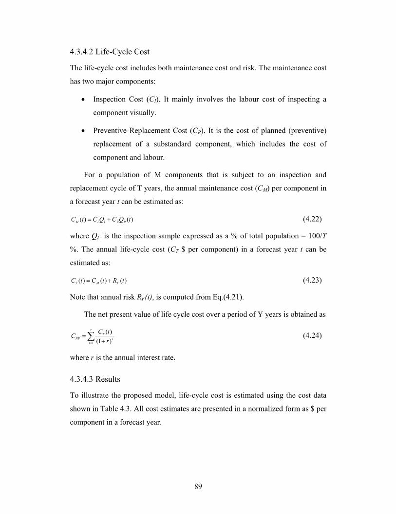
89

4.3.4.2 Life-Cycle Cost

The life-cycle cost includes both maintenance cost and risk. The maintenance cost

has two major components:

• Inspection Cost (CI). It mainly involves the labour cost of inspecting a

component visually.

• Preventive Replacement Cost (CR). It is the cost of planned (preventive)

replacement of a substandard component, which includes the cost of

component and labour.

For a population of M components that is subject to an inspection and

replacement cycle of T years, the annual maintenance cost (CM) per component in

a forecast year t can be estimated as:

)()( tQCQCtC RRIIM += (4.22)

where QI is the inspection sample expressed as a % of total population = 100/T

%. The annual life-cycle cost (CT $ per component) in a forecast year t can be

estimated as:

)()()( tRtCtC FMT += (4.23)

Note that annual risk RF(t), is computed from Eq.(4.21).

The net present value of life cycle cost over a period of Y years is obtained as

∑= +

=Y

tt

TNP r

tCC1 )1(

)( (4.24)

where r is the annual interest rate.

4.3.4.3 Results

To illustrate the proposed model, life-cycle cost is estimated using the cost data

shown in Table 4.3. All cost estimates are presented in a normalized form as $ per

component in a forecast year.

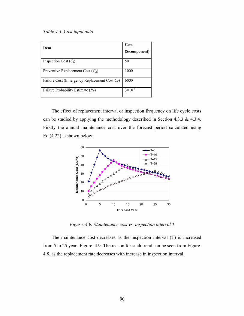
90

Table 4.3. Cost input data

Item Cost

($/component)

Inspection Cost (CI) 50

Preventive Replacement Cost (CR) 1000

Failure Cost (Emergency Replacement Cost CF) 6000

Failure Probability Estimate (PF) 3×10-3

The effect of replacement interval or inspection frequency on life cycle costs

can be studied by applying the methodology described in Section 4.3.3 & 4.3.4.

Firstly the annual maintenance cost over the forecast period calculated using

Eq.(4.22) is shown below.

0

10

20

30

40

50

60

0 5 10 15 20 25 30

Forecast Year

Mai

nten

ance

Cos

t ($/

Uni

t)

T=5T=10T=15T=25

Figure. 4.9. Maintenance cost vs. inspection interval T

The maintenance cost decreases as the inspection interval (T) is increased

from 5 to 25 years Figure. 4.9. The reason for such trend can be seen from Figure.

4.8, as the replacement rate decreases with increase in inspection interval.

91

0

1

2

3

4

5

6

7

0 5 10 15 20 25 30

Forecast Year

Ann

ual R

isk

($/U

nit) T=25

T=15T=10T=5

Figure. 4.10. Risk vs inspection interval T

The annual risk increases with increase in inspection interval as shown in

Figure. 4.10. Because longer interval means a larger number of substandard

components are vulnerable to failure. It must be stressed that the risk estimates are

highly sensitive to the annual probability of failure of a substandard component,

which is taken as 3×10-3 per year.

0

10

20

30

40

50

0 5 10 15 20 25 30

Forecast Year

Life

Cyc

le C

ost (

$/U

nit)

T=5T=10T=15T=25

Figure. 4.11. Life cycle cost vs inspection interval T

The variation of life cycle cost, which is a sum of the maintenance cost and

risk Eq.(4.23), and its net present value is shown in Figure. 4.11, which is

qualitatively similar to the variation of maintenance cost shown in Figure. 4.9.

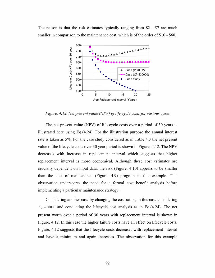
92

The reason is that the risk estimates typically ranging from $2 - $7 are much

smaller in comparison to the maintenance cost, which is of the order of $10 - $60.

400

450

500

550

600

650

700

750

800

0 5 10 15 20 25

Age Replacement Interval (Years)

Life

cycl

e C

ost (

NPV

ove

r 30

year

Case (Pf=0.02)Case (Cf=$30000)Case study

Figure. 4.12. Net present value (NPV) of life cycle costs for various cases

The net present value (NPV) of life cycle costs over a period of 30 years is

illustrated here using Eq.(4.24). For the illustration purpose the annual interest

rate is taken as 5%. For the case study considered as in Table 4.3 the net present

value of the lifecycle costs over 30 year period is shown in Figure. 4.12. The NPV

decreases with increase in replacement interval which suggests that higher

replacement interval is more economical. Although these cost estimates are

crucially dependent on input data, the risk (Figure. 4.10) appears to be smaller

than the cost of maintenance (Figure. 4.9) program in this example. This

observation underscores the need for a formal cost benefit analysis before

implementing a particular maintenance strategy.

Considering another case by changing the cost ratios, in this case considering

30000=FC and conducting the lifecycle cost analysis as in Eq.(4.24). The net

present worth over a period of 30 years with replacement interval is shown in

Figure. 4.12. In this case the higher failure costs have an effect on lifecycle costs.

Figure. 4.12 suggests that the lifecycle costs decreases with replacement interval

and have a minimum and again increases. The observation for this example

93

suggests that there is an optimal replacement interval of 13 years based on

minimum life cycle costs for maintenance.

It has been shown that the risk estimates are also sensitive to the annual

probability of failure, another case is considered where the annual probability of

failure of a substandard component as 2×10-2. Similar calculations on lifecycle

costs from Eq.(4.24) is done using the same input data from Table 4.3. The plot

on lifecycle cost over a period of 30 year is shown in Figure. 4.12 with

replacement interval on x-axis. The lifecycle costs here have a interesting profile

and suggests an optimal replacement interval of 8 years. In this example for lower

replacement interval the replacement costs dominate but in the later part when the

replacement interval is high the failure costs dominate.

4.3.4.4 Summary

A probabilistic model is presented for the estimation of maintenance cost, risk and

life-cycle cost associated with a maintenance program that involves sequential

inspection based component replacement strategy.

As a general rule, increasing the inspection interval decreases the

maintenance cost at the expense of increasing risk.

The time-dependent variation of life-cycle cost depends on the relative

magnitude of risk and cost over time.

The ratio of component failure cost to replacement cost (CF/CR) is a critical

parameter. The cost ratio should be sufficiently high, otherwise the benefit of the

maintenance program would be less than the associated cost.

The risk and cost estimates presented here are considered illustrative, the

input data pertaining to costs of inspection, replacement and failure of a

distribution component can be arrived from field experts to get a more meaningful

results. The estimation of probability of component failure must be refined

through the statistical analysis of historical component failure data and/or

structural reliability analysis of component structure.

94

4.4 Model Based on Renewal Theory

4.4.1 Introduction

A probabilistic method proposed by Van Noortwijk and Klatter, (2004) is

presented to estimate the fraction of substandard component replacement in the

distribution network based on current component demographics and lifetime

distribution estimated from the inspection data. The results are then compared to

the non-renewal case developed in Section 4.3.2.

The component replacement is assumed to follow discrete renewal process.

The probabilistic method predicts the expected number of component

replacements per unit time, which is the annual rate of components reaching

substandard state in a specified year. The assumptions in renewal process for

replacements are that the substandard components are detected and replaced in a

short period.

A discrete renewal process {N(t), t=1,2,3,…} is a non-negative integer-

valued stochastic process that registers the successive renewals in the time

interval (0, t]. The renewal times T1, T2, T3,…, is assumed to be non-negative

independent and identically distributed with discrete probability function given as

)0,,|1()0,,|(}Pr{ baiFbaiFpiT ik −−=== (4.25)

,...,2,1=i where pi represents the probability of a renewal in unit time i. This

probability function is a discrete Weibull distribution. The conditional probability

that the life time X exceeds x given X>y is given as

{ } ( )⎪⎭

⎪⎬⎫

⎪⎩

⎪⎨⎧

⎥⎦⎤

⎢⎣⎡+⎥⎦

⎤⎢⎣⎡−=−=>>

aa

by

bxybaxFyXxXP exp,,|1| (4.26)

The probability of a renewal of an aged component in future time x with

current age y can be calculated using Eq. (4.26). The expected number of

renewals for a new component is given as a recursive equation according to Van

Noortwijk (2003)

95

[ ]∑=

−+=n

ii inNEpnNE

1)]([1)]([ (4.27)

for ,...3,2,1=n and 0)0( ≡N . This equation is based on the condition that the first

renewal occurred at time Ti. The expected long term average number of renewals

per unit time is given as

μ11)]([lim

1

==

∑∞

=

∞→

ii

nipn

nNE (4.28)

which is the reciprocal of mean lifetime μ . As ∞→n , the expected long term

average cost per unit time approaches μ/c , where c is the cost associated with

each renewal and is assumed as constant with time. The developed methodology

can also be extended for a component which has aged 0≥y . The probability

distribution of residual lifetime can be discrete as

{ }),,|1(),,|(

)(|ybaiyFybaiyF

yqyiTP i

−+−+===

(4.29)

for ,...3,2,1=i . The expected number of renewals in the time interval (0, n] when

the first component has age y is given as

[ ]∑=

−+=n

ii inNEyqynNE

1)]([1)()],(~[ (4.30)

where )]([ nNE is given by Eq. (4.27). and ),(~ ynN is called the delayed renewal

process since the process starts at component age y. The expected cost of

replacement from an aged population with current component ages myy ,...,1 can

be obtained as

∑=

=m

jjj ynNEcnKE

1)],([)]([ (4.31)

where cj is the cost of replacing the jth component. The expected cost of

component replacement in unit time i can be obtained as

niiKEiKE ,...,1)],1([)]([ =−− (4.32)

96

For a unit cost of component replacement, Eq. (4.32) gives the rate of component

replacement per unit time.

4.4.2 Results

Considering the population demographics and the estimated lifetime distribution

as presented in Table 4.4, the replacement cost of the population per unit time in

future can be calculated.

Table 4.4. Statistical input data for illustrative example

Item Average (years)

Standard Deviation

(years)

Distribution Type

Age Distribution 30 15 Weibull

Lifetime Distribution 40 10 Weibull

The average age of the remaining population is 30 years and the average

lifetime of the component is 40 years. Assuming that all age components are

replaced with a new component with unit cost (c=1). The expected replacement

cost per unit time or the expected number of renewals per unit time for the

population can be calculated from Eq. (4.32) which is shown in Figure 4.13. The

year zero is the current year and Figure 4.13 shows the predictions for a forecast

period of 150 years. Figure 4.13 shows the expected cost of replacement per year

for the population as a function of current component age.

97

Figure 4.13: Expected cost of replacements per year as a function of age

The expected cost of replacements over all ages is shown in Figure 4.14.

Figure 4.14 shows the expected cost of replacements per year over all ages of the

population. The uncertainty in second replacement time is greater than the

uncertainty in first replacement time. This kind of replacement is also termed as

corrective replacement. The annual rate and hence the cost of corrective

replacement policy can be shown by Figure 4.13 & Figure 4.14. It can be shown

from Figure 4.14, that the expected number of replacements per year converges to

0.025 which is equal to the expected long term average number of replacements

(1/μ=0.025) as given in Eq. (4.28).

98

0 50 100 1500

0.01

0.02

0.03

0.04

0.05

Year

Exp

ecte

d co

st /y

ear

Figure 4.14: Expected cost of replacements per year among all ages

It is interesting to compare the result in Figure 4.14 to the non-renewal case

shown in Figure. 4.5, since they predict the same replacement rate until around 20

years. The expected replacement rate decreases as the population ages but

increases later with failure from first renewals and then converges to a constant

replacement rate with subsequent renewals. Whereas in non-renewal case (Figure.

4.5) the expected replacement rate decreases as there are no renewals.

4.4.3 Summary

A probabilistic model is presented for the estimation of the annual replacement

rate of the population and the expected replacement cost per unit time. The

component replacements are modeled as a renewal process, where a substandard

component is replaced by a new component. For the component maintenance

management, the annual rate of replacement and hence the replacement costs per

year are crucial in optimizing the maintenance actions by minimizing the life

cycle costs.

99

4.5 Imperfect Preventive Maintenance

4.5.1 Background

Let a component with lifetime variable “T” be maintained to reduce the risk of

failure. To minimize the risk of failure, preventive maintenance is performed at

regular intervals. There are two kinds of preventive maintenance (PM), namely

proactive and reactive. Proactive preventive maintenance (PPM) is done before

the initiation of degradation such that the time of initiation is delayed. Reactive

preventive maintenance (RPM) is done after the initiation of degradation such that

the rate of degradation is reduced. In this section RPM is discussed in the case of

component maintenance optimization. Essential maintenance or refurbishment is

done after a component has failed. Generally, the cost of refurbishment is very

high compared to the cost of PM. Therefore, PM actions are necessary to reduce

the cost of refurbishment. If PM actions are more frequent maintenance costs

increases, thereby reducing the refurbishment costs. Likewise, when PM actions

are less frequent, maintenance costs are less but refurbishment costs increase.

Therefore, there is a need for optimizing the number of PM actions over a

component lifetime.

With preventive maintenance (RPM), a component is either as good as new

(Perfect PM) or the rate of degradation is reduced (Imperfect PM). In case of

perfect PM, the degradation of the component starts as if the component is new,

this need not be true in reality. The effect of imperfect PM can be modeled as a

virtual age model with a degree of imperfection (γ). Maintenance generally refers

to as preventive maintenance in subsequent sections.

4.5.2 Virtual Age Model

A component with lifetime distribution )(tFT is considered by periodically

maintaining at intervals pt . After the first preventive maintenance, the

degradation of the component is reduced by the introduction of a virtual age to the

component. The concept of virtual age has been thoroughly discussed in the

100

literature and has its applications in a variety of probabilistic models (Pham and

Wang, 1996). The virtual age after first maintenance action )(1 tv is given as

ppp ttttttv 2)1()(1 <<−−= γ (4.33)

where pt is the time of first maintenance and γ is degree of maintenance

imperfection ( 10 ≤≤ γ ). In case of perfect maintenance (i.e γ =0), the virtual age

ptttv −=)(1 starts from zero age. In case of no maintenance (i.e γ =1), the virtual

age ttv =)(1 is the same as the component age t. The virtual age model can then

be used to derive the component survival function as

pp

pT

TpT

tv

t

t

tv

tv

t

t

ttt

tStvS

tS

duuhduuh

duuhduuhtS

p

p

p

p

p

2

)())((

)(

)(exp)(exp

)()(exp)(

1

)(

0

)(

)(0

1

1

1

<<

×=

⎟⎟

⎠

⎞

⎜⎜

⎝

⎛−×

⎟⎟⎠

⎞⎜⎜⎝

⎛−=

⎟⎟

⎠

⎞

⎜⎜

⎝

⎛−−=

∫∫

∫∫

γ

γ

(4.34)

where )(tST is the component survival function without maintenance. When there

is no maintenance done on the component (i.e γ =1), the survival function results

in )()( tStS Tt p= , the original survival function. In the case of perfect

maintenance (i.e γ =0), the survival function is given by

)()()( pTpTt ttStStSp

−×= (4.35)

The methodology can be generalized for any number of preventive

maintenance actions over the lifetime of the component. The virtual age of the

component after j number of maintenance actions can be given as

pppj tjtjtjtttv )1()1()( +<<−−= γ (4.36)

The component survival function after j number of preventive maintenance

actions can be derived in the same way as done in Eq(4.34).

( )( ) pp

pT

jTj

i pT

pTt tjtjt

tjStvS

tiStiS

tSp

)1()())((

)1(])1(1[

)(1

+<<×⎪⎭

⎪⎬⎫

⎪⎩

⎪⎨⎧

−

−+= ∏

= γγγ

(4.37)

101

When there is no maintenance done on the component (i.e γ =1), the survival

function results in )()( tStS Tt p= , the original survival function. In the case of

perfect maintenance (i.e γ =0), the survival function after jth PM is given by

[ ] )()()( pTj

pTt jttStStSp

−×= (4.38)

The survival probability as shown in Eq. (4.38) is greatly improved with frequent

preventive maintenance when compared with no maintenance. Even with frequent

preventive maintenance actions the survival probability decreases with time but

rather slowly as compared to no maintenance.

The effect of imperfect preventive maintenance on survival probability is

derived as in Eq. (4.37) and is very useful in maintenance optimizations decisions.

The application of imperfect maintenance in maintenance optimization is

illustrated by an example in the next section.

4.5.3 Illustrative Example

To illustrate the effect of imperfect preventive maintenance on component

survival probability, a component with a mean lifetime of 36 years following

Weibull distribution with shape parameter 3 and scale parameter 40 is considered.

The component is maintained periodically at the interval ( pt ) of 10 years. Three

scenarios of imperfect maintenance are considered here. In the first case, the

component is maintained perfectly (i.e γ =0), the second case when the component

is maintained imperfectly with γ =0.2 and the third when no maintenance work is

done (i.e γ =1). For all the three cases the survival probability function is plotted

in Figure 4.15 over 100 years. Figure 4.15 clearly shows the improvement in

survival probability in the case of perfect maintenance and the effect of imperfect

maintenance on the component survival.

102

0 20 40 60 80 1000

0.1

0.2

0.3

0.4

0.5

0.6

0.7

0.8

0.9

1

No PMImperfect PMPerfect PM

Time

Sur

viva

l Pro

babi

lity

tp=10, γ=0

tp=10, γ=0.2

Weibull(3,40), γ=1

tp→ PM Interval

γ→ Degree of PM Imperfection

Figure 4.15: Survival probability curves in case of imperfect maintenance

The model can be used to quantify the effect of maintenance imperfection on

component survival for life cycle management. The model can be used for each

component in the system or the lifetime distribution of the whole system. The

models flexibility can be exploited in various types of maintenance actions and to

vary the effect of maintenance at each interval. Finally, the model can be helpful

especially in component or system lifecycle management.

4.5.4 Cost Optimization

The effect of preventive maintenance of a system with lifetime of 100 years is

studied by Yang et al. (2006). The survival function of the system is defined by a

Weibull distribution with shape parameter 2.86 and scale parameter 94.34. The

effect of preventive maintenance on the system is modeled according to Eq(4.37).

Preventive maintenance actions are applied periodically at time intervals pt of 2,

5, 10, 15, 20, 25, 30, 40, 50, 75 and 100 years. Yang et al. (2006) demonstrated

the effect of perfect preventive maintenance to the problem described above. The

103

analysis conducted in this section extends this approach for the case of imperfect

preventive maintenance actions.

The unit cost of failure is considered as 100 and the maintenance cost is varied to

study for various cost ratios. The failure costs are calculated based on the

probability of failure at the end of system lifetime of 100 years. The maintenance

costs are calculated based on the number of maintenance actions at the end of

system lifetime. Hence, the total cost at the end of system lifetime of 100 years is

taken as the sum of failure cost and maintenance cost. The optimal maintenance

interval is found to be the maintenance interval that leads to lowest total cost

among all maintenance intervals considered.

0

20

40

60

80

0 0.2 0.4 0.6 0.8 1 1.2COST RATIO

OPT

IMA

L TO

TAL

EXPE

CTE

D C

OST

Perfect PM

Imperfect PM (γ=0.2)

OMI=15

OMI=20

30

40

40

Without Maintenance

Cost Ratio =Maintenance Cost/Failure CostOMI = Optimal Maintenance Interval

Weibull LifetimeMean = 84 YearsAnalysis period = 100 yearsFailure cost = 100

69.3

Figure 4.16: Optimal preventive maintenance

The optimal maintenance policy of the system for the various cost ratios

considered is shown in Figure 4.16. The plot shows the effect of imperfect

maintenance for two scenarios. The results from Figure 4.16 suggest that there is

less effect on the optimal maintenance intervals but there is a significant

difference in the optimal cost. Figure 4.16 illustrates the concept of an imperfect

preventive maintenance model in maintenance optimization of systems.

104

4.6 Conclusions

The effect of maintenance actions can be quantified using probabilistic models for

life cycle costs and equipment performance. This chapter discusses such

application of maintenance models through the probabilistic approach, using

component lifetime distributions.

Age-based replacement policy is simple and effective to implement in a

system with a large population of relatively inexpensive components. An optimal

age-based refurbishment policy for wood pole management is presented. For a

cost ratio of CP/CF = 0.2, the optimal replacement age is estimated at 40 years. An

interesting conclusion is that the type of lifetime distribution (Weibull, Gompertz

or Log-logistic) has a limited sensitivity to the optimum replacement age and the

expected life-cycle cost.

A sequential inspection-based replacement model is proposed to manage

components from a large distribution network. The model is demonstrated to

show the effect of an inspection interval in estimating the maintenance cost, risk,

and life cycle costs. This approach is applicable to distributed populations in

which inspections are scheduled as blocks of the populations. This approach is

computationally complex and needs realistic cost input data to support decision

making. As a general rule, increasing the inspection interval decreases the

maintenance cost at the expense of increasing risk. The time-dependent variation

of life-cycle cost depends on the relative magnitude of risk and cost over time.

A rather simplistic approach, in which components are replaced as they are

detected to be in substandard state (Corrective Replacement), is demonstrated

using renewal theory. The component replacement policy from renewal theory

framework is presented in estimating the future expected replacement costs.

A probabilistic lifetime model is proposed to consider the effect of imperfect

preventive maintenance on systems and components. The model has the

flexibility to incorporate the imperfections of maintenance actions using the

concept of virtual age. The model can consider the effect of maintenance

imperfections at various maintenance intervals. The effect of imperfect preventive

105

maintenance in maintenance optimization is illustrated. The results show that

imperfect preventive maintenance increases optimal total costs and the frequency

of optimal maintenance intervals.

106

CHAPTER 5 STOCHASTIC MODEL FOR PITTING CORROSION

IN STEAM GENERATORS

5.1 Background

The Steam generators (SG) are the most critical component of nuclear power

reactor next to reactor core as shown in Figure 5.1. They are large heat

exchangers that use the heat from primary coolant to produce steam in secondary

side that is sent to steam turbines to produce electricity. A nuclear power plant

may have multiple steam generators that are of shell-and-tube type heat

exchangers each consisting of several thousand tubes. The steam generator tubes

function as part of the nuclear reactor primary heat transport system pressure

boundary. These tubes are generally thin walled for efficient heat transfer from

primary side to the secondary side. In order to act as an effective barrier these

tubes should be free of cracks, perforations and general degradation.

Figure 5.1: CANDU nuclear power plant (from http://canteach.candu.org/)

However in the past the steam generator tubes have experienced widespread

degradation as observed at nuclear power plants [IAEA, 1997]. The degradation

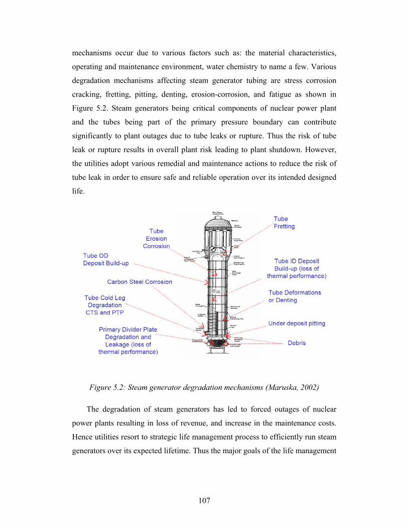
107

mechanisms occur due to various factors such as: the material characteristics,

operating and maintenance environment, water chemistry to name a few. Various

degradation mechanisms affecting steam generator tubing are stress corrosion

cracking, fretting, pitting, denting, erosion-corrosion, and fatigue as shown in

Figure 5.2. Steam generators being critical components of nuclear power plant

and the tubes being part of the primary pressure boundary can contribute

significantly to plant outages due to tube leaks or rupture. Thus the risk of tube

leak or rupture results in overall plant risk leading to plant shutdown. However,

the utilities adopt various remedial and maintenance actions to reduce the risk of

tube leak in order to ensure safe and reliable operation over its intended designed

life.

Figure 5.2: Steam generator degradation mechanisms (Maruska, 2002)

The degradation of steam generators has led to forced outages of nuclear

power plants resulting in loss of revenue, and increase in the maintenance costs.

Hence utilities resort to strategic life management process to efficiently run steam

generators over its expected lifetime. Thus the major goals of the life management

108

strategies are to avoid surprises, learn from experience and manage the investment

in steam generators (Tapping et al., 2000) in the most optimal way.

The methodology in implementing life management strategies is to first

characterize the possible degradation mechanisms effecting the steam generator

life and reliability. In order to achieve this, a sound fitness-for-service (FFS) plan,

and good inspection capability is important. The possible remedial and

maintenance actions are then assessed based on their merits in extending the

service life of steam generator. The maintenance actions are then ranked based on

risk reduction and cost effectiveness. However, even with best efforts on effective

maintenance strategies uncertainties still lie with the aging of steam generators.

The uncertainties also associated with how the flaws are characterized, detected,

and mitigated. The success of life management strategies depend on minimizing

these uncertainties. A risk based approach is therefore critical to life management

strategies for its success. Such approach accounts for various uncertainties and

quantifies them through probabilistic models for better decision making.

Pitting corrosion is a predominant form of degradation on the outside

diameter (OD) of steam generator tubing of some nuclear power plants. This

Chapter discusses the application of stochastic models for pitting corrosion

degradation towards steam generator life cycle management.

5.1.1 Pitting Corrosion

During the course of normal operation of a nuclear power plant the impurities

from make up water, the condenser leaks and the corrosion product oxides

leached from feed train structural materials are carried along the feed water and

get deposited over the steam generator surfaces. These deposits lead to problems

such as under deposit pitting, tube failures and loss of production. The regions

near the sludge pile at tube sheet and support plate experience crevice like

conditions which favour pitting corrosion.

The pits are characterised as wide mouthed, dish shaped with low aspect ratio

which could be described as localised wastage. Pitting corrosion typically occurs

109

at locally weak spots on tube where the passive layer breaks creating a local

corrosion cell which is promoted by the presence of chloride and sulphate ions.

The impurities such as sulphates and chlorides are produced from condenser leaks

and chemicals used in chemical cleaning which result in local acidic conditions

favourable to pitting process. The pitting process is accelerated in the presence of

oxidizing conditions and copper deposits (IAEA, 1997). The accumulations of

sludge act as barrier to diffusion accelerating the pitting process by enhancing

chemical concentration.

The redox potential of the solution should exceed a critical value for the pits

to initiate. This potential can be achieved by the presence of dissolved oxygen,

oxidizing metal cations like FeCl3 or CuCl3 of higher redox potential than critical

potential are more conducive to rapid pitting than dissolved oxygen. Any

movement in the solution can remove the local concentration of Cl- and H+ ions

that is required to continuous propagation thereby stopping pitting (Burstein et al.,

1994). Laboratory studies and field observations have shown that the pitting rate

could be very high resulting in through wall failure in a matter of days (Angell,

2002).

Severe pitting has been experienced in SG tubes in some nuclear reactors.

Pitting observed in CANDU unit is described as under deposit pitting corrosion

which is contributed due to presence of porous adherent deposits. The utility

adopt aggressive water lancing and chemical cleaning to remove most of the

deposits thereby mitigating pitting. Lancing uses high pressure jets to

mechanically remove sludge from tube surfaces. By periodic lancing the depth of

sludge is kept at reasonable levels. More advanced lancing equipment is used with

multidirectional pressurized water jets which could remove tenacious sludge

deposits (IAEA, 1997). Chemical cleaning is always preceded by water lancing

such that they allow cleaning chemicals to access the crevices.

5.1.1.1 Chemical Cleaning

The sludge and deposits consist of feedtrain corrosion products (e.g., Fe3O4,

Fe2O3, Cu, Cu2O, CuO), impurities from condenser cooling water (e.g., SiO2), and

110

water treatment chemicals (e.g., sodium phosphate). The chemical cleaning

process commonly used is based on EPRI-SGOG (Electric Power Research

Institute – Steam Generator Owners’ Group) which is generally applied during

plant outage (Semmler et al., 1998). If Cu is present an oxidizing step is applied

whereas a reducing step dissolves Fe oxides. Of the various chemical cleaning

formulations, the EDTA (Ethylene Diamine Tetra Acetic Acid) formulations are

more popular in chemical cleaning of steam generators (Padma et al., 2001). The

composition of chemical cleaning formulation consists of additives added to

EDTA such as pH additive, reducing agent, oxidizing agent, and corrosion

inhibitors. The compositions and conditions of chemical cleaning process are

usually specific for a particular SG depending on the materials used and operating

environment. Such chemical cleaning process has successfully been implemented

by power utilities in extending the life of steam generators (Evans et al., 2002,

Maruska, 2002).

5.1.1.2 Eddy Current Inspection

The most common tool for in-service inspection of SG tubing are eddy current

probes which consists of small electrical coil enclosed in the probe head

connected to an electric circuit. Eddy current probes are electro-magnetically

coupled to the test specimen and generate eddy currents flowing in a direction

parallel to the coil windings. An eddy current signal results from the disturbance

in the magnetic field caused by the defect interfering with the eddy currents

generated by the probe as it scans the defect. The amplitude and phase of the

signal reflect the amplitude and phase of the affected part of the three dimensional

eddy current field. The signal has a characteristic pattern that is used in

identifying the type of defect.

The two basic types of eddy current probes used in SG inspection are

“impedance” and “transmit-receive”. The eddy current signals measured from the

primary coil electric impedance induced by the eddy current magnetic field are of

the impedance probes. In a transmit-receive (T/R) probe, the transit coil generates

magnetic field and the eddy current signals are measured as the change in voltage

111

induced in the receive coil. The transmit-receive probe has proved to have a

greater scope in eddy current testing and is currently used in most modern probes

(Obrutsky, L., 2002).

Eddy current signal parameters are affected mainly by

• Tube thickness

• Defect type, size and orientation

• Test frequency of coil

• Magnetic properties of the material

The eddy current amplitude decays exponentially with depth from the surface

of the probe and phase lag increases linearly with depth. The frequency of the test

coil is selected based on the thickness of the tube, resistivity and permeability of

tube material. It is quite common to use multiple frequencies on the same coil to

test the probe characteristics (probe calibration) and also in characterizing various

types of defects. Eddy current signals from a single coil are actually absolute

measurements and are so called absolute probes. The differential probe consists of

two coils side by side that measure the differential signal which is much sensitive

to defects and insensitive to slowly varying properties like gradual dimensional or

temperature variations and probe wobble. It’s also common to have both absolute

and differential setup in the same probe taking advantage of each. The three

common types of probes used at CANDU steam generator tube inspection

discussed in this Chapter are Carter-1, Carter 2 - Cecco 4, and X - Probe. There

are a number of eddy current probes developed for specific applications and

defect characteristics.

5.1.1.2.1 Carter-1 Bobbin Probe

The CTR-1-350, or Carter 1 probe uses absolute and differential bobbin coils that

are coaxial with the inspected tube. The induced eddy current flows

circumferentially in the steam generator tube, parallel to the coil windings. Hence

these probes are not sensitive to circumferentially oriented defects. Bobbin probes

are very good at volumetric defects. The volumetric material loss at a given

112

location is estimated by comparing the probe signal to amplitude calibration

curves. The signal amplitude is sensitive to the morphology and circumferential

extent of the flaw which could lead to potential sizing error. The main advantage

of the bobbin probe is its speed which allows inspection in a short period of time

thereby reducing unavailability and outage times.

5.1.1.2.2 Carter 2 - Cecco 4 Transmit-Receive Probe

The CTR2-C4, or Carter 2 – Cecco 4 probe is a multi-coil (array) transmit/receive

eddy current probe, consisting of small coils aligned in the axial direction along

the probe. Similar to the CTR-1 probe, the CTR2-C4 probe is generally not

sensitive to degradation modes such as circumferential cracking, however it can

detect multiple volumetric flaws such as corrosion pits at the same axial location

around the circumference of the tube. Because of the multi-coil design, the CTR2-

C4 probe has been shown to detect corrosion pits with higher accuracy, with

negligible change in operational speed.

5.1.1.2.3 Transmit-Receive type X-Probe

The X-probe is a fast single-pass transmit/receive eddy current probe that

combines the circumferential and axial modes in a single probe head. X-probe has

a number of transmit/receive coils varying from 8 to 18 depending on probe

diameter. The probe has a scanning speed comparable to the standard bobbin

probes that is able to discriminate between axial, circumferential, and volumetric

flaws in a single scan. X-probe is used in field recently and is only used at

specific sections which need attention. X-probe is believed to characterize defects

better than other probes available as it has greater resolution and stores lots of

information on tube characteristics since it has more number of coils.

5.1.2 LCM Strategies

The goal of the steam generator life cycle management is to maximize value

while ensuring safe and reliable operation until the expected end of life. The

purpose of life cycle management plan is to provide both near term and short term

strategies for inspection, cleaning, and modifications necessary for safe and

113

reliable operation. The objectives and scope of LCM plans is discussed in Chapter

Chapter 2. In this section LCM strategies currently implemented in steam

generator corrosion management is discussed.

5.1.2.1 Current LCM Strategies

The current steam generator remedial actions include extensive cleaning

campaigns with the use of specialized water lancing equipment at low and high

temperature chemical cleaning. Enhanced inspection is essential for an effective

maintenance strategy. Advanced inspection technique such as X-probe is used for

more rapid and accurate inspections. Degraded tubes are removed for

metallographic assessments and fitness for service evaluations. Particular

attention is given to chemistry control with improved water treatment plants and

condenser. The copper components from the feedtrain and condenser are replaced.

Much emphasis is given in maintaining chemistry specifications in secondary side

chemistry within guidelines while maintaining high hydrazine chemistry regime.

Currently work is undergoing on the development of tube sleeving in repairing the

plugged tubes.

5.1.2.2 Fitness for Service Assessment

A sound fitness for service program is essential in characterizing degradation

mechanisms. Fitness for service guidelines are therefore developed for each plant

since the degradation mechanisms vary for each plant. Fitness for service

assessment along with structural integrity and operational assessment is

conducted at each inspection campaign to demonstrate the ability of steam

generator to function safely until next inspection outage. The utility considers the

primary objective of fitness for service is same as life cycle management; to

assure the integrity of steam generators as a primary pressure and containment

boundary, the difference being the time span of application.

5.1.2.3 LCM Issues

The utilities were successful in mitigating pitting degradation with aggressive

cleaning campaigns and efficient chemistry control. Despite the remedial actions

114

new pits initiate and continue to grow rapidly. This presents a major challenge for

steam generator LCM in predicting future equipment performance, estimating the

remaining life, and the adverse economic consequences. The ageing of steam

generator under pitting corrosion is not fully understood. Uncertainties also exist

on how the flaws are characterized, detected and mitigated. A risk based approach

is therefore essential for efficient life cycle management program which accounts

for various uncertainties and to quantify them. A probabilistic based framework

for pitting corrosion degradation is discussed in next section based on eddy

current inspection data.

5.2 Stochastic Modelling of Pitting Corrosion

5.2.1 Introduction

The risks associated with steam generator tube pitting corrosion can be quantified

through stochastic modelling. Estimating the expected number of tubes that

require plugging and the probability of tube leakage in the future operating period

are important input to risk based life-cycle management of steam generators

(Harris, et al., 1997). When the extent of pitting is unacceptable, then the need for

maintenance activities such as water lancing or chemical cleaning should be

assessed in a risk-based framework. The model should be able to assess the

impact of maintenance interval on the risk associated with the event of tube

leakage and be able to carry out the cost benefit analysis. In technical terms,

answering these questions requires distributions pit size, and rate of new pit

generation. The objective of this study is to discuss various uncertainties with

inspection data and develop probabilistic models to estimate probability

distributions from existing inspection data and apply them to life cycle

management.

5.2.1.1 Pit Generation Models

Localized pitting corrosion process is considered to have stochastic character in

nature. Existing models are developed in idealized setting which utilizes

laboratory data obtained from continuous monitoring of pit initiation and

115

propagation using potentiometers. As passivation breaks down, the potential

difference increases sharply. This potential (pitting potential) depends on the

nature and composition of the solution. Likewise the time interval needed to

observe the drastic increase in potential is taken as the induction time. Stochastic

models based on the statistical distribution of pitting potential and induction times

for pit formation are proposed from such experimental observations (Shibata,

1996; Mola et al., 1990; Wu et al., 1997). The process of pit generation is

modelled as a pure birth stochastic model. Opposite to pit formation, passive layer

healing operates as a pit death process. These models are useful in investigating

the experimental procedures in electrochemical systems. Such models may not be

applicable in field applications because it’s not practical to monitor the pitting

potential in steam generator tubes.

Markov process model for the growth of maximum pit depth was discussed

by Provan and Rodriguez, (1989) applied to oil and gas pipelines where corrosion

is a very slow process. Hong, (1999) proposes the use of combined model by

representing the pit generation process with Poisson model and the pit depth

growth process by Markov process. The combined model is reported to give

better estimate for the problems discussed by Provan and Rodriguez, (1989).

These models are not directly applicable in analyzing pitting problems in steam

generator for the reasons discussed in Section 5.1.1.

Pit generation and growth is fairly rapid in some CANDU reactors. It is

believed oxygen intake during shut down and start-up cycles promotes the pitting,

which is a kind of inter-granular attack. The time of rapid growth is random and

then growth stops. There is evidence to suggest that most pits don’t grow after

this initial period of generation and growth. Thus pit size also becomes a random

variable. Such a process is also referred to as marked point process as shown in

Figure 5.3.

116

0

10

20

30

40

50

60

70

80

90

100

0 1 2 3 4 5 6 7 8 9 10

Time (Years)

Pit D

epth

(%tw

)T

T → Random Variable

Figure 5.3: Plot to illustrate marked point process for pits > 50%tw

Model pit initiation is random in time and pit assumes a random size from a

distribution. Small size pits can not be reliably detected or measured. The focus of

attention is on relatively large pits of size (≥ 50% tw). The idea is that pits

exceeding a relatively high threshold (50%) follow the Poisson process as shown

in extreme value theory (Smith, 2004). The pit generation is assumed to follow

Poisson process which falls under stochastic birth process. The pit generation

model following NHPP is discussed in next section along with parameter

estimation from observed inspection data.

5.2.2 Stochastic Pit Generation

Let the number of pits N(t) in the interval [0-t] follow a Non-Homogenous

Poisson Process (NHPP) with intensity function )(tλ . The mean value function

)(tΛ or the expected number of pits E[N(t)] per SG following Weibull Power law

is given as (Ross, 2000)

∫ ==Λ=t

tdssttNE0

)()()]([ β

βαλ (5.1)

The parameters α, is a scale parameter and β is the shape parameter. When shape

parameter β=1, the intensity function is constant and the process is defined as a

Homogeneous Poisson process (HPP).

117

5.2.3 Inspection Process

In practice it is quite difficult and uneconomical to inspect the equipment

continuously with time. Inspection of equipment is usually conducted at periodic

or non periodic inspection time intervals. Consider an inspection process of a

single SG from the start of its operation as shown in Figure 5.4, where non-

destructive inspections are conducted at times t1, t2, t3 and t4.

10

4

0

6

0

2

4

6

8

10

12

t1 t2 t3 t4Time, t

Cor

rosi

on P

its

Figure 5.4: SG pitting corrosion inspection data

The number of pits observed at time t2 is the number of new pits generated

during the interval [t1-t2]. The number of pits generated during inspection interval

[t1-t2] follows a Poisson distribution which is given as

{ } 1212)]()([

12 ,0!

)]()([)()( 12 ttnn

ttentNtNPn

tt >≥Λ−Λ

==− Λ−Λ− (5.2)

If at the time of inspection t3 there are no observed new pits, such kind of

data are called censored data. The censored data gives us the information that

there are no new pits observed in the interval [t2-t3] with probability given as

{ } 23)]()([

23230)()( ttetNtNP tt >==− Λ−Λ− (5.3)

By assuming a probability model for pit generation rate, the probability of

observing these pits in an inspection process as shown in Figure 5.4 is calculated

by a likelihood method. The parameters of the model are then estimated by

maximizing this likelihood function. The theory and methodology of likelihood

118

method is explained further in subsequent sections. The advantage of likelihood

method is that it can handle censored data.

5.3 Estimation of Pit Generation Rate

From inspection data, the number of pits generated in different intervals can be

obtained as shown in Figure 5.4 throughout the service life of the system.

Suppose in a kth interval [tk1-tk2], nk pits are generated and that there are in

total M intervals for which data are available. The maximum likelihood function

for this sample can be set up as (Lawless, 2003):

{ })]()([exp!

)]()([),( 12

1

12kk

M

k k

nkk tt

ntt

Lk

Λ−Λ−Λ−Λ

=∏=

βα (5.4)

By substituting the mean rate function, the log-likelihood is derived as

{ } { }∑=

⎥⎦

⎤⎢⎣

⎡−−⎟⎟

⎠

⎞⎜⎜⎝

⎛−∝

M

kkkkkk ttttnl

11212log),( ββββ

βα

βαβα (5.5)

The unknown parameters are estimated from the conditions of maximization as

{ }

{ } { } { }[ ] 0loglog1loglog),(

01),(

11211222

12

1122

112

=−−−−⎥⎦

⎤⎢⎣

⎡−

−−

=∂

∂

=⎥⎦

⎤⎢⎣

⎡−−=

∂∂

∑

∑

=

=

M

kkkkkkk

kk

kkkkk

M

ikk

k

tttttttt

ttttnl

ttnl

ββββββ

ββ

ββ

ββα

βββα

βααβα

(5.6)

The parameters βα ˆ,ˆ can be estimated by trial and error from Eq. (5.6).

Standard maximization codes can also be applied to Eq. (5.5) to estimate the

parameters. The Fisher information matrix is derived as the negative of the second

derivative of the log likelihood function with respect to the parameters. The

asymptotic covariance matrix of the maximum likelihood estimators is an inverse

of the Fisher information matrix. Using the estimates of asymptotic variance, the

approximate confidence limits for the distribution parameters can be obtained

under the assumption of normality.

119

5.3.1 Test for Homogenous Poisson process

In case of the HPP model (β=1), the pit generation rate is constant with time. A

statistical test, such as the likelihood ratio test, can be applied to test the null

hypothesis that β=1. The likelihood ratio statistic (LRS) is given as

{ }),1(),1(2 0011 αβαβ =−≠−= llLRS (5.7)

where ),1( 00 αβ =l and ),1( 11 αβ ≠l are the log likelihood functions for the

homogeneous and non-homogeneous Poisson process models, respectively. The

LRS follows the Chi-square distribution with one degree of freedom. The null

hypothesis is rejected at the 5 % level of significance when p-value is less than

5%, and it can be concluded that the pit generation rate is not constant or

otherwise.

5.4 Extreme Pit Depth Model

5.4.1 Pit Depth Distribution

The pit depths are measured using NDE techniques which are used to evaluate

flaw distribution in tubes. The measured pit depths pose challenge in modeling

probability distribution as they are associated with detection uncertainty and

measurement error. Measured pit depths of size less than 30% through wall depth

(TWD) is based on expert judgment due to relatively small size of pits for a tube

of wall thickness in range of 1-2 mm. All new pits greater than 50% TWD is

considered for the analysis as the measurement error effects are minimal to larger

pits. Pit depths exceeding a threshold of 50% TWD can be treated as extreme (or

peaks) of the pit generation process. The distribution of these peaks over the

threshold can be modeled using the generalized Pareto distribution (GPD),

commonly used in the extreme value theory (Smith, 2004). The generalized

Pareto distribution (GPD) for peaks over thresholds ( ux > ) is given by

ξ

σξ

/1

11)( ⎟⎠⎞

⎜⎝⎛ −−−=

uxxFX (5.8)

120

where σ is the scale parameter and ξ is the shape parameter. When 0≤ξ , the

GPD has a long and unbounded tail. When 0>ξ , the distribution is right

bounded at ξσ / . In the limiting case when 0→ξ the distribution takes

exponential with mean equal to σ . When 1=ξ , GPD model becomes the

uniform distribution. The GPD model is commonly used in extreme value

analysis of engineering and environmental systems (Smith, 2004).

The distribution parameters can be estimated by method of moments using

the sample mean (m) and standard deviation (s) computed from the pit depth data

based on the following relations (Hosking and Wallis, 1987)

⎥⎥⎦

⎤

⎢⎢⎣

⎡−⎟

⎠⎞

⎜⎝⎛ −

= 121 2

sumξ (5.9)

( )( )ξσ +−= 1um (5.10)

5.4.2 Extreme Pit Depth Distribution

In order to estimate probability of the tube leakage in a steam generator, the

distribution of the largest (extreme) pit size is required. Since the pit occurrence is

described by a non-homogeneous Poisson (Weibull) process, the rate of

occurrence of pits exceeding a size z at time t is given as

)](1)[()( zFtt Xz −= λλ (5.11)

The expected number of pits exceeding depth >z % TWD in the interval [0-t] per

SG, i.e, the mean rate function, is given as

[ ])(1)()()]([ zFtttNE Xzz −Λ=Λ= (5.12)

The distribution of the number of these large pits is given by the Poisson

distribution as

)}(exp{!)]([)( t

ntnP z

nz

N Λ−Λ

= (5.13)

From the principles of extreme value theory, the distribution of the largest pit

among all generated n pits in [0-t] can be expressed as

121

)}(exp{)]}(1)[(exp{!

)]([)]([)(0

)(

tzFtn

etzFzF zXn

tnn

XY Λ−=−Λ−=Λ

= ∑∞

=

Λ−

(5.14)

The distribution )(zFY is also referred to as the Generalized Extreme Value

(GEV) distribution, which encompasses all three limiting forms of the extreme

value distributions, namely, the Gumbel, Frechet and Weibull distributions (Smith,

2004). It can be used to estimate the probability of tube leakage per operating year.

If the reactor unit has n number of SGs, each with leak probabilities iLp

acting as a series system independent of each other, then the probability of having

a leak in the unit ULp can be calculated as

∏=

−−=n

iL

UL i

pp1

)1(1 (5.15)

The number of extreme pits for the Unit is actually a sum of independent

Poisson processes from all SGs. The expected number of extreme pits with depth

z % TWD in the interval [0-t] per unit can be calculated as

)]([...)]([)]([)]([21

tNEtNEtNEtNEnzzzz +++= (5.16)

The expected number of extreme pits per unit can be used in developing unit

life-cycle management plans.

5.5 Gamma Frailty Poisson Model

The Poisson models discussed earlier in the preceding sections are proposed in the

context of pitting corrosion process. The pitting observed from a single SG is

usually in negligible amount considering large pits. Pitting processes from all the

SGs in a reactor unit are assumed as realizations from a random pitting process

model of a single SG. It is quite reasonable to pool the data from all the SGs of a

reactor unit to model the random pitting process of a single SG. However the

unobserved randomness among the different SGs can be accounted for using

frailty model. Such frailty Poisson models are used in demographic studies such

as in panel count data (Lawless, 1987, Zhang and Jamshidian, 2003). The frailty

model on Poisson process is defined as

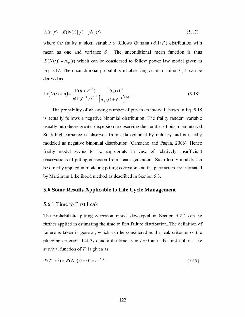
122

)()|)(()|( 0 ttNEt Λ==Λ γγγ (5.17)

where the frailty random variable γ follows Gamma ( δδ /1, ) distribution with

mean as one and variance δ . The unconditional mean function is thus

)())(( 0 ttNE Λ= which can be considered to follow power law model given in

Eq. 5.17. The unconditional probability of observing n pits in time [0, t] can be

derived as

( ) [ ][ ] 11

10

01

1

)(

)()(!

)()(Pr −− +−−

−

+Λ

Λ

Γ

+Γ==

δδ δδδδ

n

n

t

tn

nntN (5.18)

The probability of observing number of pits in an interval shown in Eq. 5.18

is actually follows a negative binomial distribution. The frailty random variable

usually introduces greater dispersion in observing the number of pits in an interval.

Such high variance is observed from data obtained by industry and is usually

modeled as negative binomial distribution (Camacho and Pagan, 2006). Hence

frailty model seems to be appropriate in case of relatively insufficient

observations of pitting corrosion from steam generators. Such frailty models can

be directly applied in modeling pitting corrosion and the parameters are estimated

by Maximum Likelihood method as described in Section 5.3.

5.6 Some Results Applicable to Life Cycle Management

5.6.1 Time to First Leak

The probabilistic pitting corrosion model developed in Section 5.2.2 can be

further applied in estimating the time to first failure distribution. The definition of

failure is taken in general, which can be considered as the leak criterion or the

plugging criterion. Let T1 denote the time from 0=t until the first failure. The

survival function of T1 is given as

)(1 )0)(()( t

zzetNPtTP Λ−===> (5.19)

123

Where )(tN z is the number of failures at time t, and )(tzΛ is the mean value

function of extreme pits. The expected time to failure can now be calculated by

integrating the survival function in Eq. (5.19).

∫∞

Λ−=0

)(1 ][ dteTE tz (5.20)

If the mean value function follows Weibull power law as shown in Eq. (5.1),

the expected time to first leak and its variance formula can be derived as shown

below.

⎟⎟⎠

⎞⎜⎜⎝

⎛+Γ⎟

⎠⎞

⎜⎝⎛=

βαβ β 11][

/1

1TE (5.21)

⎥⎦

⎤⎢⎣

⎡⎟⎟⎠

⎞⎜⎜⎝

⎛+Γ−⎟⎟

⎠

⎞⎜⎜⎝

⎛+Γ⎟

⎠⎞

⎜⎝⎛=

ββαβ β 1121][ 2

/2

1TVar (5.22)

Considering the generalized Pareto distribution for the pit depth as discussed

in Section 5.4.1 and NHPP model for pit generation discussed in Section 5.2.2,

the time to first leak distribution can be estimated as

ξβ

σξ

βα /1

1

1 )(⎟⎠⎞

⎜⎝⎛ −−−

=>uz

tetTP (5.23)

5.6.2 Time to nth Failure/Leak

The probabilistic corrosion pitting model can be used in estimating the time to nth

failure distributions. Let nS denote the time until failure n for ,...,2,1=n where

00 =S . The distribution of nS is given by

∑−

=

Λ−Λ=−≤=>

1

0

)(

!)(

)1)(()(n

tzzn e

tntNPtSP

ν

ν

ν (5.24)

The expected time to nth failure can be calculated by integrating the survival

function Eq. (5.22) which is given as

∫∑∞ −

=

Λ−Λ=

0

1

0

)(

!)(

][ dtet

SEn

tzn

z

ν

ν

ν (5.25)

124

Considering the generalized Pareto distribution for the pit depth discussed in

Section 5.4.1 and NHPP model for pit generation discussed in Section 5.2.2, the

time to nth failure distribution can be estimated as

∑−

=

⎟⎠⎞

⎜⎝⎛ −−−⎥

⎥⎦

⎤

⎢⎢⎣

⎡⎟⎠⎞

⎜⎝⎛ −−

=>1

0

1

/1

/1

!

1

)(n uz

t

n e

uzt

tSPν

σξ

βα

νξβ

ξβ

ν

σξ

βα

(5.26)

5.7 Uncertainties Associated with Pit Depth Model

Eddy current (ET) inspection process is aimed to produce reliable information for

engineers to ensure structural integrity of SG. However there are various

uncertainties involved in each stage of inspection process that hinders the overall

reliability of ET inspection process. The major reliability issues of eddy current

inspection relevant for engineers are the detectability and accuracy issues. It is

required that defects greater than critical size should be detected by ET

inspection. The detectability issue is addressed using Probability of Detection

(POD) curves for the technique as well as for analysis/analyst. The major factors

that affect POD are

• Probe sensitivity to defect orientation

• Human factors

• Poor signal to noise ratio

• Material characteristics

• Probe wear

• Internal and external deposits

• Scan rate

Most of the factors discussed above are minimized by selecting an

appropriate probe and better inspection procedures. Even with the best efforts in

minimizing the uncertainties there still lies a residual uncertainty that constitute

toward inspection reliability. It is therefore necessary to demonstrate the POD

curves for the inspection process along with the inspection results.

125

Sizing accuracy reveal how close the technique defect size match to that of

true defect size. The sizing accuracy is addressed by means of root mean squared

error (RMSE) by comparing eddy current measurements to that of the actual

depths from a pulled tube. The major factors affecting the accuracy of eddy

current technique are

• Defects on Calibrated tube may not depict actual defects on field

• Probe wear

• Signal to noise ratio

• Human factors

Most of the factors can be minimized by selecting an appropriate probe and

by customizing calibration standards. As discussed above for detection

uncertainty, it is difficult eliminate uncertainties completely. It is therefore

necessary to demonstrate the sizing accuracy of the inspection process along with

the eddy current inspection results.

The effects of sizing accuracy and detectability are minimized when

considering relatively larger pit depths. The effect of sizing accuracy on pit depth

distribution is illustrated in Section 5.8. The pit depths with size ≥50%tw are

considered for modelling the depth distribution. Generalized Pareto distribution is

considered for modelling pit depths exceeding a threshold of 50%tw as discussed

in Section 5.4.1.

5.7.1 Measurement Error Analysis from Field Inspections

The probabilistic model for pit depth should take into account the measurement

error in Non-destructive test (NDT) tool. Statistical methods have been used for

evaluation of measurement error from such NDT tools by laboratory studies. The

statistical methods applicable in Non-destructive evaluation (NDE) are reviewed

by Olin&Meeker (1996) and Sweeting (1995). They show the application of

regression models on the measured flaws and the true flaws in characterizing the

measurement errors of NDT tools. Inspection data on flaws using multiple NDT

tools can also be used in characterizing the measurement error of each tool. In this

126

section such application in nuclear steam generator tubes non-destructive

inspection are discussed.

Non-destructive inspection of steam generator tubes has played a major part

in its safe and successful operation. Periodic inspection database on SG tubes

reveal corrosion pit depth measurements from various eddy current probes. In

some cases corrosion pits are measured using multiple probes to gain more insight,

especially on larger pit depths which could potentially leak. The corrosion pit

depth data measured from multiple eddy current probes can be used to quantify

the measurement error for each measuring probe. The EPRI guidelines for

inspection of SG only refer to root mean squared error/differential (RMSE/D) in

accessing the quality of an inspection instrument. The methodology discussed

here follows the paper from Morrison, et al. (2002) where he discusses the

application of Grubbs Method from multiple inspection data.

5.7.1.1 Estimation of Measurement Errors from Inspection Data for Each of

Two Probes

The root mean squared error/differential (RMSE/D) calculates the total scatter

from the two tools being compared. If the measured values from Probe 1 and

Probe 2 are xi and yi, the RMSE/D is calculated as

∑=

−=n

iii yx

nDRMSE

1

2)(1/ (5.27)

From RMSE/D it is not possible to decompose the total scatter and assign it to

each tool. This approach is helpful only if one of the measuring probe is assumed

to be perfect. In most of the cases this approach penalizes bad probe unnecessarily

by assigning the total scatter to bad probe.

5.7.1.2 Grubbs Method

Grubbs (1948) suggested the use of sample variance and covariance to estimate

measurement errors for individual probes. The measured pit depths (xi, yi) from

each probe is assumed to follow the model given as

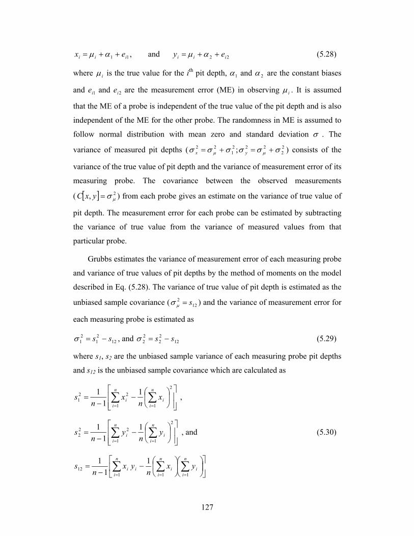
127

2211 and, iiiiii eyex ++=++= αμαμ (5.28)

where iμ is the true value for the ith pit depth, 1α and 2α are the constant biases

and 1ie and 2ie are the measurement error (ME) in observing iμ . It is assumed

that the ME of a probe is independent of the true value of the pit depth and is also

independent of the ME for the other probe. The randomness in ME is assumed to

follow normal distribution with mean zero and standard deviation σ . The

variance of measured pit depths ( 22

2221

22 ; σσσσσσ μμ +=+= yx ) consists of the

variance of the true value of pit depth and the variance of measurement error of its

measuring probe. The covariance between the observed measurements

( [ ] 2, μσ=yxC ) from each probe gives an estimate on the variance of true value of

pit depth. The measurement error for each probe can be estimated by subtracting

the variance of true value from the variance of measured values from that

particular probe.

Grubbs estimates the variance of measurement error of each measuring probe

and variance of true values of pit depths by the method of moments on the model

described in Eq. (5.28). The variance of true value of pit depth is estimated as the

unbiased sample covariance ( 122 s=μσ ) and the variance of measurement error for

each measuring probe is estimated as

1221

21 ss −=σ , and 12

22

22 ss −=σ (5.29)

where s1, s2 are the unbiased sample variance of each measuring probe pit depths

and s12 is the unbiased sample covariance which are calculated as

⎥⎥⎦

⎤

⎢⎢⎣

⎡⎟⎠

⎞⎜⎝

⎛−

−= ∑∑

==

2

11

221

11

1 n

ii

n

ii x

nx

ns ,

⎥⎥⎦

⎤

⎢⎢⎣

⎡⎟⎠

⎞⎜⎝

⎛−

−= ∑∑

==

2

11

222

11

1 n

ii

n

ii y

ny

ns , and (5.30)

⎥⎦

⎤⎢⎣

⎡⎟⎠

⎞⎜⎝

⎛⎟⎠

⎞⎜⎝

⎛−

−= ∑∑∑

===

n

ii

n

ii

n

iii yx

nyx

ns

11112

11

1

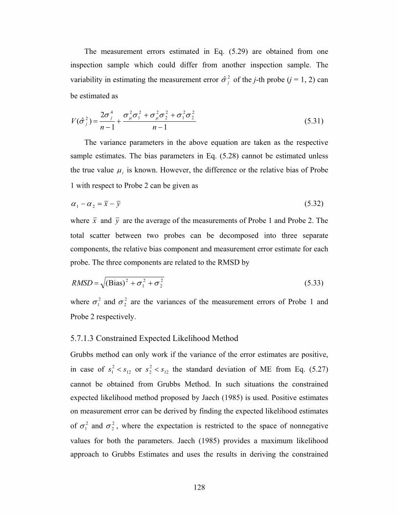
128

The measurement errors estimated in Eq. (5.29) are obtained from one

inspection sample which could differ from another inspection sample. The

variability in estimating the measurement error 2ˆ jσ of the j-th probe (j = 1, 2) can

be estimated as

112

)ˆ(22

21

22

221

242

−

+++

−=

nnV j

j

σσσσσσσσ μμ (5.31)

The variance parameters in the above equation are taken as the respective

sample estimates. The bias parameters in Eq. (5.28) cannot be estimated unless

the true value iμ is known. However, the difference or the relative bias of Probe

1 with respect to Probe 2 can be given as

yx −=− 21 αα (5.32)

where x and y are the average of the measurements of Probe 1 and Probe 2. The

total scatter between two probes can be decomposed into three separate

components, the relative bias component and measurement error estimate for each

probe. The three components are related to the RMSD by

22

21

2)Bias( σσ ++=RMSD (5.33)

where 21σ and 2

2σ are the variances of the measurement errors of Probe 1 and

Probe 2 respectively.

5.7.1.3 Constrained Expected Likelihood Method

Grubbs method can only work if the variance of the error estimates are positive,

in case of 1221 ss < or 12

22 ss < the standard deviation of ME from Eq. (5.27)

cannot be obtained from Grubbs Method. In such situations the constrained

expected likelihood method proposed by Jaech (1985) is used. Positive estimates

on measurement error can be derived by finding the expected likelihood estimates

of 21σ and 2

2σ , where the expectation is restricted to the space of nonnegative

values for both the parameters. Jaech (1985) provides a maximum likelihood

approach to Grubbs Estimates and uses the results in deriving the constrained

129

expected likelihood estimates for measurement error. The MLE of ( )22

21 σσ + is S

which is the total scatter given by

nsssn

S)2)(1( 12

22

21 −+−

= (5.34)

The CEL estimators are considered such that they lie in the first quadrant on

the line ( ) S=+ 22

21 σσ in a proportion v such that

S

vvS

v

v

)1(

10;22

21

νσ

σ

−=

≤≤= (5.35)

The CEL estimate of measurement error is then derived as the weighted

average with respect to likelihood in the transformed space as defined in Eq.

(5.35). The expressions for the CEL estimate of measurement error as given by

Jaech (1985) are

21

22

1

021 ˆˆ;ˆ σσσ −== S

ISI

(5.36)

where

[ ] 2/12

22

2221

1

01

1

00

)1(2)1()(

)(

)(

nsvvssvf

dvvfI

dvvvfI

−−++−=

=

=

∫

∫

νν

(5.37)

Morrision (2002) suggests that the CEL estimates have to be checked to see if

they are reasonable and they also suggest that when the covariance between the

Probes is negative the CEL estimate does not seem appropriate.

5.8 Effect of Measurement Error and POD on Pit Depth

Distribution

The main objective of this section is to illustrate the effect of uncertainty in

detectability and measurability of pit depths or flaw depths in general. The source

of such uncertainties in eddy current inspection process is already discussed in

130

Section 5.7. This section covers the technical details in accounting for

measurement error and probability of detection.

The pit depths observed from eddy current inspection are associated with

uncertainties with inspection process and tools. In addition to measurement error

and probability of detection the pit depths are also associated with censoring. Due

to the inherent noise from the eddy current probe, pit depths with sizes <30%

TWD cannot be measured and hence designated as censored observations. Such

uncertainties on pit depth greatly effect the predictions on the leak probability

estimates. Simulation study is conducted to quantify the effect of uncertainties in

pit depth measurements.

5.8.1 Simulation Analysis

Considering that the true pit depths follows exponential distribution with mean

15% TWD. The probability density function of the true pit depth is shown in

Figure 5.5.

0.0%

0.5%

1.0%

1.5%

2.0%

2.5%

3.0%

3.5%

4.0%

4.5%

5.0%

0 20 40 60 80 100Pit Depth (%TWD)

Prob

abili

ty D

ensi

ty (P

DF)

Figure 5.5: Probability density plot for true pit depth

The event of interest to most utilities is the probability of tube leak and the

number of tubes plugged in a given outage. The tube leak probability is associated

with the probability of pit depth exceeding 95% TWD. The number of tubes

plugged is associated with the probability of pit depth exceeding 51% TWD. The

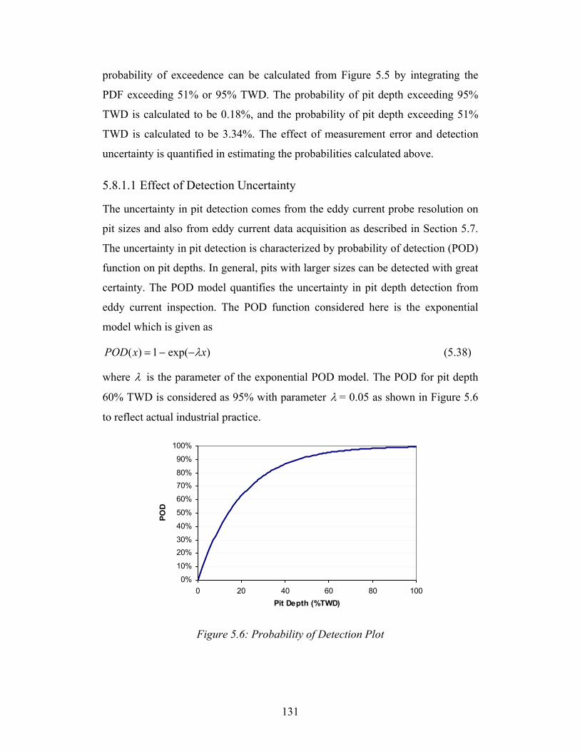
131

probability of exceedence can be calculated from Figure 5.5 by integrating the

PDF exceeding 51% or 95% TWD. The probability of pit depth exceeding 95%

TWD is calculated to be 0.18%, and the probability of pit depth exceeding 51%

TWD is calculated to be 3.34%. The effect of measurement error and detection

uncertainty is quantified in estimating the probabilities calculated above.

5.8.1.1 Effect of Detection Uncertainty

The uncertainty in pit detection comes from the eddy current probe resolution on

pit sizes and also from eddy current data acquisition as described in Section 5.7.

The uncertainty in pit detection is characterized by probability of detection (POD)

function on pit depths. In general, pits with larger sizes can be detected with great

certainty. The POD model quantifies the uncertainty in pit depth detection from

eddy current inspection. The POD function considered here is the exponential

model which is given as

)exp(1)( xxPOD λ−−= (5.38)

where λ is the parameter of the exponential POD model. The POD for pit depth

60% TWD is considered as 95% with parameter λ = 0.05 as shown in Figure 5.6

to reflect actual industrial practice.

0%

10%

20%30%

40%

50%

60%

70%80%

90%

100%

0 20 40 60 80 100Pit Depth (%TWD)

POD

Figure 5.6: Probability of Detection Plot

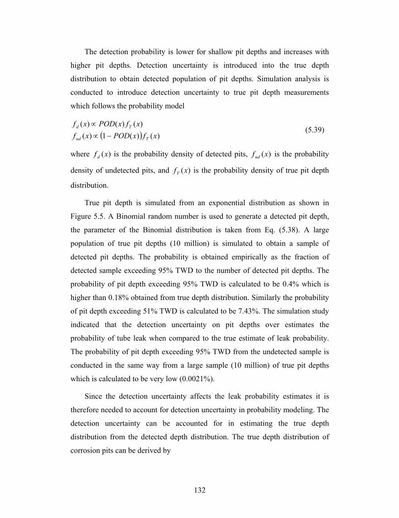
132

The detection probability is lower for shallow pit depths and increases with

higher pit depths. Detection uncertainty is introduced into the true depth

distribution to obtain detected population of pit depths. Simulation analysis is

conducted to introduce detection uncertainty to true pit depth measurements

which follows the probability model

( ) )()(1)()()()(

xfxPODxfxfxPODxf

Tud

Td

−∝∝

(5.39)

where )(xf d is the probability density of detected pits, )(xfud is the probability

density of undetected pits, and )(xfT is the probability density of true pit depth

distribution.

True pit depth is simulated from an exponential distribution as shown in

Figure 5.5. A Binomial random number is used to generate a detected pit depth,

the parameter of the Binomial distribution is taken from Eq. (5.38). A large

population of true pit depths (10 million) is simulated to obtain a sample of

detected pit depths. The probability is obtained empirically as the fraction of

detected sample exceeding 95% TWD to the number of detected pit depths. The

probability of pit depth exceeding 95% TWD is calculated to be 0.4% which is

higher than 0.18% obtained from true depth distribution. Similarly the probability

of pit depth exceeding 51% TWD is calculated to be 7.43%. The simulation study

indicated that the detection uncertainty on pit depths over estimates the

probability of tube leak when compared to the true estimate of leak probability.

The probability of pit depth exceeding 95% TWD from the undetected sample is

conducted in the same way from a large sample (10 million) of true pit depths

which is calculated to be very low (0.0021%).

Since the detection uncertainty affects the leak probability estimates it is

therefore needed to account for detection uncertainty in probability modeling. The

detection uncertainty can be accounted for in estimating the true depth

distribution from the detected depth distribution. The true depth distribution of

corrosion pits can be derived by

133

∫∞

==

∝

0 )()(

;)(

)(1)(

)()(

)(

dxxPOD

xfk

xPODxf

kxf

xPODxf

xf

ddT

dT

(5.40)

where )(xf d is the probability density of detected pits and )(xfT is the

probability density of true pit depth distribution and k is a normalizing constant.

The mean and variance of the true pit depth distribution can be calculated as

∫

∫ ∫∞

∞ ∞

−=

==

0

22

0 0

)()(

)()(1)(

dxxfx

dxxPOD

xfk

xdxxxf

TTT

dTT

μσ

μ (5.41)

Similarly, the distribution of the undetected pit depths can be derived using

the probability of detection concept which is given as

( )

( ) ( )∫∞

−=−=

−∝

0

)()(1);()(11)(

)()(1)(

dxxfxPODkxfxPODk

xf

xfxPODxf

TuTu

ud

Tud

(5.42)

where )(xfud is the probability density of undetected pits and )(xfT is the

probability density of true pit depth distribution and uk is a normalizing constant.

The mean and variance of the undetected pit depth distribution can be calculated

as

( )

∫

∫ ∫∞

∞ ∞

−=

−==

0

22

0 0

)()(

)()(11)(

dxxfx

dxxfxPODk

xdxxxf

ududud

Tu

udud

μσ

μ (5.43)

Considering the detected pit depth distribution and probability of detection

(POD) function from Eq. (5.38), the probability density function for true pit depth

and undetected pit depths can be estimated.

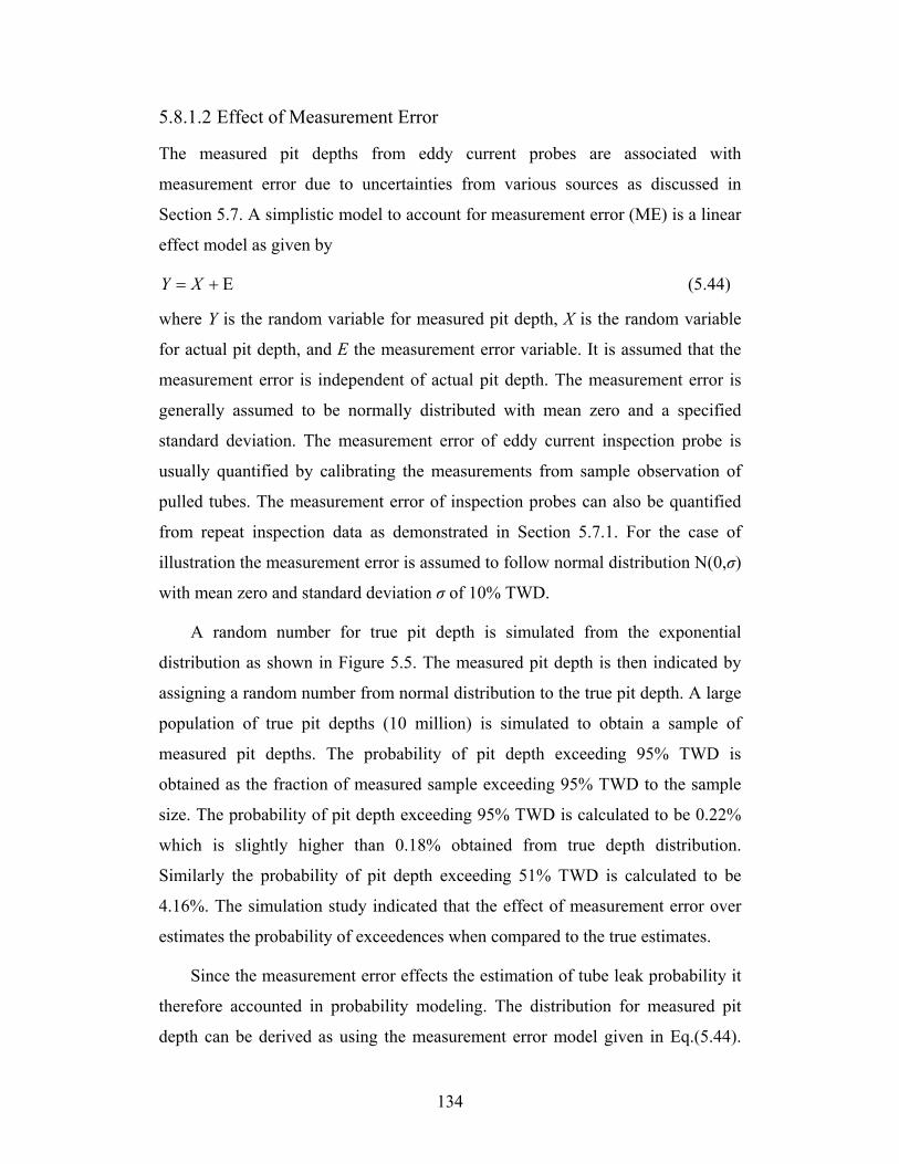
134

5.8.1.2 Effect of Measurement Error

The measured pit depths from eddy current probes are associated with

measurement error due to uncertainties from various sources as discussed in

Section 5.7. A simplistic model to account for measurement error (ME) is a linear

effect model as given by

Ε+= XY (5.44)

where Y is the random variable for measured pit depth, X is the random variable

for actual pit depth, and E the measurement error variable. It is assumed that the

measurement error is independent of actual pit depth. The measurement error is

generally assumed to be normally distributed with mean zero and a specified

standard deviation. The measurement error of eddy current inspection probe is

usually quantified by calibrating the measurements from sample observation of

pulled tubes. The measurement error of inspection probes can also be quantified

from repeat inspection data as demonstrated in Section 5.7.1. For the case of

illustration the measurement error is assumed to follow normal distribution N(0,σ)

with mean zero and standard deviation σ of 10% TWD.

A random number for true pit depth is simulated from the exponential

distribution as shown in Figure 5.5. The measured pit depth is then indicated by

assigning a random number from normal distribution to the true pit depth. A large

population of true pit depths (10 million) is simulated to obtain a sample of

measured pit depths. The probability of pit depth exceeding 95% TWD is

obtained as the fraction of measured sample exceeding 95% TWD to the sample

size. The probability of pit depth exceeding 95% TWD is calculated to be 0.22%

which is slightly higher than 0.18% obtained from true depth distribution.

Similarly the probability of pit depth exceeding 51% TWD is calculated to be

4.16%. The simulation study indicated that the effect of measurement error over

estimates the probability of exceedences when compared to the true estimates.

Since the measurement error effects the estimation of tube leak probability it

therefore accounted in probability modeling. The distribution for measured pit

depth can be derived as using the measurement error model given in Eq.(5.44).

135

The conditional distribution on measured pit depth given the distribution of actual

pit depth can be obtained as

)|Pr()(| xXxyyF XY =−<Ε= (5.45)

The marginal distribution of observed pit depth can then be obtained as

∫∞

⎟⎠⎞

⎜⎝⎛ −

Φ=0

)()( dxxfxyyF XY σ (5.46)

Similarly the probability density function for observed pit depth can be obtained

as

∫∞

⎟⎟⎠

⎞⎜⎜⎝

⎛ −−=

02

2

)(2

)(exp21)( dxxfxyyf XY σσπ

(5.47)

The probability of observing n number of pit depths from eddy current inspection

is given by the likelihood function given as

∏ ∫=

∞

⎪⎭

⎪⎬⎫

⎪⎩

⎪⎨⎧

Θ⎟⎟⎠

⎞⎜⎜⎝

⎛ −−=Θ

n

iX

i dxxfxy

L1 0

2

2

);(2

)(exp

21),(

σσπσ (5.48)

The parameters of the likelihood function can then be estimated by

maximizing the logarithm of likelihood function using standard maximization

routines. The distribution of actual detected pit depth distribution can be estimated

by likelihood method as described in this section.

5.8.1.3 Combined Effect of Detection and Measurement Error Uncertainty

In actual field measurement the pit depths are usually associated with detection

uncertainty and measurement error of the eddy current inspection process. In this

simulation study the true pit depth distribution considered in Figure 5.5 is

introduced with probability of detection (POD) and measurement error as

discussed in previous sections. Detection uncertainty is introduced first as the

POD in Eq. (5.36) is defined on the true pit depth to obtain detected pit depths

which is then introduced with measurement error. A large sample (10 million) of

true pit depths is simulated by introducing detection uncertainty and measurement

error to obtain a realistic sample of detected pit depths. The probability of pit

136

depth exceeding 95% TWD is obtained empirically as the fraction of detected

sample exceeding 95% TWD to the number of detected pit depths. The

probability of pit depth exceeding 95% TWD is calculated to be 0.51% which is

higher than 0.18% obtained from true depth distribution. Similarly the probability

of pit depth exceeding 51% TWD is calculated to be 9.02%.

0.18%0.22%

0.41%

0.51%

0.0%

0.1%

0.2%

0.3%

0.4%

0.5%

0.6%

TRUE ME POD POD+ME

Prob

abili

ty o

f exc

eedi

ng 9

5% T

WD

Figure 5.7: Effect of pit depth uncertainties on probability of pit depth exceeding

95% TWD

3.34%4.16%

7.43%

9.02%

0%

2%

4%

6%

8%

10%

TRUE ME POD POD+ME

Prob

abili

ty o

f exc

eedi

ng 5

1% T

WD

Figure 5.8: Effect of pit depth uncertainties on probability of pit depth exceeding

51% TWD

The effect of pit depth uncertainties on estimating the probability of

exceeding 95 % TWD is shown in Figure 5.7. The results indicate that the

137

uncertainty in detection (POD) and measurement error (ME) over estimates the

true estimate of the probability of exceedences. It is therefore required to account

for measurement error and probability of detection on pit depths in probability

modeling.

5.8.2 Remarks

The event of interest in the context of life cycle management is the probability of

tube leak which results in forced outage and the number of tubes plugging. In

order to estimate the tube leak probability from eddy current inspection data it is

required to account for uncertainties in pit depth measurements. In this section a

simulation study is conducted to estimate the effect of uncertainties in pit depths

towards estimation of probability of pit depth exceeding 95% or 51% TWD. The

results indicate that the measurement error and detection uncertainties over

estimate the exceedence probabilities when compared to the estimate from true pit

depth distribution. The uncertainties in pit depth measurements are therefore

needed to account for in probability modeling. The section also discusses the

probability models in accounting for such uncertainties in estimating the true pit

depth distribution.

5.9 Inspection Uncertainty in Modeling Pitting Corrosion of

Steam Generators

Due to costs involved in eddy current inspection of SG tubes it is not economical

to conduct frequent inspections. Usually the SG tubes are either partially

inspected every 2-4 years or more frequently depending on the extent of aging SG

tubes. Such situations limit the amount of data required to model the random

pitting process of a particular SG. The detected pit depths from eddy current

inspections are also associated with probability of detection, measurement error

and censoring of pit depths. Corrosion pits with depth ≤ 30% TWD cannot be

measured accurately due to inherent noise in eddy current probes and therefore

indicated as censored pit depths. Such uncertainties in inspection process hinder

the estimation of realistic tube leak probability.

138

5.9.1 Simulation Analysis

The standard practice in industry is to plan a scheduled outage every two years.

For a reactor unit the number of SGs inspected usually depends on the extent of

degradation in SGs. For the simulation study conducted in this section the reactor

unit is considered to have 12 SGs each experiencing similar pitting corrosion

degradation process. Hence the data from the SGs inspected are grouped to model

the uncertainty in corrosion pitting process for a single SG. The objective of this

study is to quantify the uncertainty in estimating the tube leak probability and

number of tubes plugged per SG under different inspection plans. The inspection

plans considered are the number of SGs (3, 6, 9, and 12) inspected every two

years.

The analysis considers a known pit generation process for a particular SG in

estimating the probability of tube leak in the next outage from the pit depth data

obtained from simulation. The pit occurrence follows a Poisson distribution with

mean rate following Weibull power law rate as discussed in Section 5.2.2. The

parameters for the SG pit generation model per SG are taken as 1.382 as scale (α)

and 2.5 as scale parameter (β) to reflect the actual observation from industry.

Assuming the process starts at year 0, the mean rate of pitting in an interval [0 t]

in a single SG for a period of 16 years is shown in Figure 5.9.

0

100

200

300

400

500

600

0 2 4 6 8 10 12 14 16Year

Mea

n Pi

t Occ

uren

ace

Rat

e

Figure 5.9: Mean pit occurrence rate plot

139

Using the Pit occurrence rate from Figure 5.9 and considering the true pit

depth distribution from Section 5.8 the extreme pit depth model from Section 5.4

is applied to estimate the mean occurrence rate of extreme pits (Eq. 5.12) and the

expected annual leak probability (Eq. 5.14) as described in Section 5.4. The tube

leak probability in next outage is calculated by considering the leak criterion (z)

as 95% TWD.

0%

2%

4%

6%

8%

10%

12%

14%

2-4 4-6 6-8 8-10 10-12 12-14 14-16 16-18Outage Interval (Year)

Prob

abili

ty o

f Tub

e Le

ak

Figure 5.10: Probability of tube leak in next outage

The probability of tube leak predicted in next outage is shown in Figure 5.10

at each inspection outage for a period of 16 years using true pit depth distribution.

The probability of tube leak prediction in outage years 2-4 is calculated as 2.5% at

outage year 2 as shown in Figure 5.10. Simulation study is conducted by

introducing the detection uncertainty and measurement error on pit depths. The

results from the analysis are then compared to the probability of tube leak in next

outage calculated from true pit depth (Figure 5.10).

140

0

1

2

3

4

5

6

7


Expe

cted

num

ber o

f Tub

es

Plug

ged

Figure 5.11: Expected number of tubes plugged in next outage

Similarly the expected number of tubes plugged predicted in next outage is shown

in Figure 5.11 at each inspection outage for a period of 16 years. The results from

the simulation analysis are then compared to the expected number of tubes

plugged in next outage calculated from true pit depth distribution as shown in

Figure 5.11.

5.9.1.1 Procedure

The inspection plans are designated as plans 1-4 for inspecting 3, 6, 9, and 12 SGs

at each inspection outage. Under an inspection plan the pit generation is simulated

using the model shown in Figure 5.9 for a period of 16 years. Since pit depth is a

random variable, the pit depths are simulated from a true pit depth distribution as

shown in Figure 5.5. Probability of detection and measurement error uncertainty

is then introduced as discussed in Section 5.8.1 to obtain a realistic detected

sample in each outage. The detected pit depth sample is then grouped from all

SGs from all previous inspection outages to estimate the pit depth distribution and

pit generation rate. The pit depth distribution is assumed to follow exponential

where the distribution parameter is estimated from maximum likelihood method

to account for censored sample with pit depth ≤ 30% TWD. A flow chart of the

simulation analysis procedure is shown in Figure 5.12. The probability of tube

leak and the number of tubes plugged for the next outage per SG are estimated at

each inspection outage.

141

Figure 5.12: Flow chart on simulation analysis procedure

Under each inspection plan 10000 simulations are conducted to obtain the

statistics on the estimate of tube leak probability and number of tubes plugged at

142

next outage. The results on probability of tube leak prediction from simulation

analysis are shown in Figures 5.13-5.16.

Inspection of 3 new boilers at each outage

0%

5%

10%

15%

20%

25%

30%

35%

40%

45%


Prob

abili

ty o

f Tub

e Le

ak

Upper 95%CLExpectedLow er 95%CLExact

Figure 5.13: Probability of tube leak prediction in next outage under inspection

plan 1


0%

5%

10%

15%

20%

25%

30%

35%

40%

45%


Prob

abili

ty o

f Tub

e Le

ak

Low er 95%CLExpectedUpper 95%CLExact


plan 2

143

Inspection of 9 boilers at each outage

0%

5%

10%

15%

20%

25%

30%

35%

40%

45%


Prob

abili

ty o

f Tub

e Le

ak

Low er 95%CLExpectedUpper 95%CLExact


plan 3

Inspection of all 12 boilers at each outage

0%

5%

10%

15%

20%

25%

30%

35%

40%

45%


Prob

abili

ty o

f Tub

e Le

ak



plan 4

The obvious result from Figures 5.13-5.16 is that, the more the number of

SGs inspected the lesser is the sampling uncertainty in estimating the leak

probability estimate. The results indicate that inspecting more than 6 SGs at each

outage provide reasonable estimates on probability of tube leak predictions. Since

the uncertainty in estimating the leak probability is mostly from the number of pit

depth measurements recorded. The results from simulation analysis in Figures

144

5.13-5.16 indicate that the uncertainty in eddy current inspection of pit depths

greatly bias the estimate on leak probability. The results indicate that the

uncertainty in pit depth measurements result in over estimating the leak

probability estimate until around year 10 and under estimating the true leak

probability estimate in the later years.

The results on predicting the number of tubes plugged from simulation

analysis are shown in Figures 5.17-5.20.


0

2

4

6

8

10

12


Num

ber o

f Tub

es P

lugg

ed


Figure 5.17: Number of tubes plugged predicted in next outage under inspection

plan 1

145


0

2

4

6

8

10

12


Num

ber o

f Tub

es P

lugg

ed



plan 2

Inspection of 9 boilers at each outage

0

2

4

6

8

10

12


Num

ber o

f Tub

es P

lugg

ed



plan 3

146

Inspection of all 12 boilers at each outage

0

2

4

6

8

10

12


Num

ber o

f Tub

es P

lugg

ed



plan 4

The sampling uncertainty in predicting the number of tubes plugged in the

next outages decreases with the number of SGs inspected as shown Figures 5.17-

5.20. But the sampling uncertainty in predicting the number of tubes plugged is

not significant when compared to the results from leak probability predictions.

The uncertainties in pit depth measurements over estimate the prediction of

number of tubes plugged in next outage when compared to exact predictions from

true pit depth distribution.

5.9.2 Remarks

The prediction of probability of tube leak in next outage is greatly biased by

uncertainties in eddy current inspection of pit depths as shown in Figure 5.21.

This result is independent of inspection plans considered. The uncertainties in pit

depth measurements over estimate the probability of tube leak prediction in next

outage until around 10 years, and under estimate the leak probability prediction in

the later years when compared to the leak probability estimate from true depth

distribution. The effect of sampling uncertainty for different inspection plans

towards probability of leak predictions is shown in Figure 5.22. The sampling

uncertainty decreases as more data is collected in each outage. The increase in

147

COV in later years as shown in Figure 5.22 is due to the expected value of leak

probability is lower in later outage interval..

0%

5%

10%

15%

20%

25%


Leak

Pro

babi

lity

Simulation

Exact

Figure 5.21: Comparison of the exact and simulation results for leak probability

0%

20%

40%

60%

80%

100%

120%


CO

V

n=3n=6n=9n=12

Figure 5.22: COV in leak probability prediction for different inspection plans

The prediction on number of tubes plugged in not greatly biased by

uncertainties in eddy current inspection of pit depths as shown in Figure 5.23.

The uncertainties in pit depths over estimate the prediction on number of tubes

plugged in next outage at in later years of inspection. The sampling uncertainty in

inspection plans is not very significant in prediction of number of plugged tubes

as shown in Figure 5.24 at least in later outage intervals.

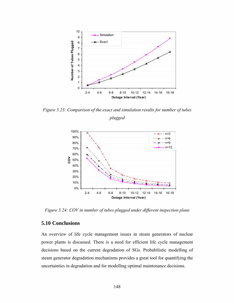
148

0

1

2

3

4

5

6

7

8

9

10


Num

ber o

f Tub

es P

lugg

ed

Simulation

Exact

Figure 5.23: Comparison of the exact and simulation results for number of tubes

plugged

0%

10%

20%

30%

40%

50%

60%

70%

80%

90%

100%


CO

V

n=3n=6n=9n=12

Figure 5.24: COV in number of tubes plugged under different inspection plans

5.10 Conclusions

An overview of life cycle management issues in steam generators of nuclear

power plants is discussed. There is a need for efficient life cycle management

decisions based on the current degradation of SGs. Probabilistic modelling of

steam generator degradation mechanisms provides a great tool for quantifying the

uncertainties in degradation and for modelling optimal maintenance decisions.

149

In the case of steam generator pitting corrosion, the rate of pit generation is

modeled as a non-homogeneous Poisson process which falls into the class of

stochastic birth process model. The pitting activity is observed during various

outages of the plant’s history by the use of eddy current inspection. The

parameters of the pit generation process are estimated by taking into account both

censored observations and non-censored observations. The pit depth distribution

exceeding a threshold pit depth is modeled as the generalized Pareto distribution

(GPD), which falls into the class of extreme value distribution. The generation of

extreme pits also follows Poisson process, with pit depth distribution following

GPD which can be characterized as a marked point process.

The results are presented from the stochastic model in estimating the

expected number of extreme pits and the annual leak probability during future

operation crucial for steam generator life management decision modelling. Some

results on probability of first leak or nth leak can be applicable to steam generator

fitness for service assessments and life cycle management planning.

The effect of measurement error and detection uncertainty in eddy current

inspections on measured defect depths is presented from simulation results. The

results indicate that the measurement error and detection uncertainties

overestimate the exceedence probabilities compared with the estimate from true

pit depth distribution. The probability models provide a framework in quantifying

the uncertainties and in estimating the true defect distribution models. The

probability model on true defect distribution is needed for a realistic estimate of

the uncertainty in pitting corrosion degradation of steam generators.

The effects of uncertainties in the eddy current inspection process for a

reactor unit are demonstrated through a simulation study. Pitting corrosion

degradation in each SG is simulated from a known stochastic model for a period

of 16 years. The pit depth measurements are introduced with uncertainties from

detection and measurement error. The censoring in pit depths is considered in

estimating the pit depth distribution from simulated observations due to threshold

limits on measuring pit depth from eddy current probes. The parameters of the

150

stochastic model are estimated by grouping the data from all SGs at an inspection

outage to predict the probability of leak and the number of tubes plugged in next

outage.

The prediction of the probability of tube leaks in next outage is greatly biased

by uncertainties in eddy current inspection of pit depths. The uncertainties in pit

depth measurements overestimate the probability of tube leak prediction in next

outage until around 10 years, and underestimate the leak probability prediction for

the later years compared with the leak probability estimate from true depth

distribution. The prediction on number of tubes plugged in not greatly biased by

uncertainties in eddy current inspection of pit depths. The uncertainties in pit

depths overestimate the prediction on number of tubes plugged in next outage in

later years of inspection. However, the sampling uncertainty in inspection plans is

not very significant in predicting the number of plugged tubes.

151

CHAPTER 6 STEAM GENERATOR LCM APPLICATION

6.1 Introduction

Previous chapter discuss the pitting corrosion model and estimation methods

applicable to steam generator life cycle management. This chapter deals with

actual field inspection data obtained from industry. The application and benefits

of the model are illustrated in the context of lifecycle management of a steam

generator. Optimization on the chemical cleaning cycle of a SG is presented.

6.2 Data Analysis

The probabilistic modelling of pitting corrosion in this chapter is based on the

reported results from eddy current inspection of several steam generators at a

nuclear generating station. The SGs considered in this study have undergone two

separate water lancing and chemical cleaning (WL/CC) campaigns in a period of

approximately eight years. Therefore, only data between two WL/CC campaigns

(i.e maintenance interval) will be used.

Only pits greater than or equal to 50% through-wall depth (TWD) observed

during maintenance interval is considered for extreme pit generation model. There

is less uncertainty in the detection of these deeper pits, and also higher confidence

in the reported depths. Furthermore, deeper pits have higher significance in the

context of steam generator LCM with regards to tube plugging and potential for

through-wall penetration.

The database provided by industry consists of 122 pits ≥ 50% TWD, and

their distribution is shown in Figure 6.1. Due to similar operating environment the

results from all SGs are considered together as one sample.

152

05

10152025303540

55 60 65 70 75 80 85 90 95 100Pit Size (%TWD)

Freq

uenc

y

Figure 6.1: Distribution of pit sizes ≥ 50% TWD

The number of new pits generated gradually increases with the time of

inspection, as shown in Figure 6.2. An increase over time is also related with the

increase in sludge that provides favourable crevice conditions for pit generation.

0

4

8

12

16

20

0 2 4 6 8Year of Inspection

Num

ber o

f New

Pits

Figure 6.2: Generation of new pits during different inspection outages

6.2.1 Model Parameter Estimation

6.2.1.1 Estimation of the Pit Generation Rate

The pit generation rate is estimated from maximum likelihood method as

described in Section 5.3 following Poisson process. The maximum likelihood

estimates of the parameters of the Poisson models are presented in Table 6.1.

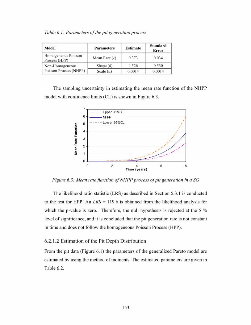
153

Table 6.1: Parameters of the pit generation process

Model Parameters Estimate Standard Error

Homogeneous Poisson Process (HPP) Mean Rate (λ) 0.373 0.034

Shape (β) 4.526 0.530 Non-Homogeneous Poisson Process (NHPP) Scale (α) 0.0014 0.0014

The sampling uncertainty in estimating the mean rate function of the NHPP

model with confidence limits (CL) is shown in Figure 6.3.

0

1

2

3

4

5

6

7

0 2 4 6 8Time (years)

Mea

n R

ate

Func

tion

Upper 95%CLNHPPLow er 95%CL

Figure 6.3: Mean rate function of NHPP process of pit generation in a SG

The likelihood ratio statistic (LRS) as described in Section 5.3.1 is conducted

to the test for HPP. An LRS = 119.6 is obtained from the likelihood analysis for

which the p-value is zero. Therefore, the null hypothesis is rejected at the 5 %

level of significance, and it is concluded that the pit generation rate is not constant

in time and does not follow the homogeneous Poisson Process (HPP).

6.2.1.2 Estimation of the Pit Depth Distribution

From the pit data (Figure 6.1) the parameters of the generalized Pareto model are

estimated by using the method of moments. The estimated parameters are given in

Table 6.2.

154

Table 6.2: Parameters of the pit depth distribution

Method Shape (ξ) Scale (σ) (% TWD)

Threshold (u) (% TWD)

Method of moments 0.509 25.51 49

R2 = 0.98

-3

-2.5

-2

-1.5

-1

-0.5

0

-6 -5 -4 -3 -2 -1 0Log[q (x)]

Log[

1-g

(x)]

Figure 6.4: The GPD probability paper plot of the pit depth data

The goodness of fit of the GPD model is investigated using the probability paper

plot. To derive axes of the probability plot, Eq. (5.8) is rewritten as

))(1(1 xFLoguxLog X−=⎟⎠⎞

⎜⎝⎛ −− ξ

σξ (6.1)

The X-axis of the plot is defined as Log(1- FX(x)) = Log(q(x)) and the Y-axis

as Log(1- g(x)), where g(x) = ξ(x - u)/σ. The sample data are plotted along these

axes, as shown in Figure 6.4. The R2 value of 0.98 confirms that the GPD model

provides a good fit to the data.

6.3 Model Application

Assessing the risk associated with tube leakage and the exceedance of the tube

plugging margin in the next operating period are important considerations for

steam generator life-cycle management. The proposed probabilistic model for

pitting corrosion can be used to answer these questions.

155

6.3.1 Probability of Tube Leak

Operational experience and other evidence suggest that a corrosion pit may leak

when its depth is of the order of 95 % TWD. Therefore, the probability of tube

leakage per SG in a time interval (0 - t) can be computed from the extreme value

distribution (Eq. 5.14) for z = 95%.

As shown by the results in Figure 6.5, the probability of tube leakage in the

early years in a SG is negligible, but it increases rapidly in later years, exceeding

1 % in the 8th year.

0.0%

0.4%

0.8%

1.2%

1.6%

0 1 2 3 4 5 6 7 8

Time (years)

Tube

Lea

kage

Pro

babi

lity

Figure 6.5: Annual probability of tube leakage in a SG

6.3.2 Tube Plugging

0

1

2

3

4

5

6

0 1 2 3 4 5 6 7 8Time (years)

Num

ber o

f Tub

es P

lugg

ed

Upper Bound

Mean

Low er Bound

Figure 6.6: Expected number of plugged tubes

156

From the proposed model, the average number of tubes to be plugged in an 8-

year interval is estimated as 3.5 tubes per SG using Eq. (5.12). Note that the

plugging limit is assumed to be equal to 51 % TWD. The sampling uncertainty in

estimating the expected number of tubes plugged is shown in Figure 6.6. In fact,

the distribution of the number of tubes plugged in an 8 year interval follows the

Poisson distribution as shown in Figure 6.7.

0%

5%

10%

15%

20%

25%

0 1 2 3 4 5 6 7 8 9 10 11 12 13 14 15

Number of Tubes Plugged

Prob

abili

ty (%

)

Figure 6.7: Distribution of the number of tubes plugged per SG

6.3.3 Time to Leak

Based on the results from pit generation rate and pit depth distribution, the time to

leak as discussed in Section 5.6 can be estimated. Considering z = 95 %TWD as

leak criterion, Eq. (5.23) gives the survival distribution for time to first leak.

( )526.4061 1028.2exp)( ttTP ××−=> − (6.2)

157

0%10%20%30%40%50%60%70%80%90%

100%

0 10 20 30 40Time (Years)

Surv

ival

Pro

babi

lity

Func

tion

Figure 6.8: Survival probability function plot for time to first leak

0%

2%

4%

6%

8%

10%

12%

0 10 20 30 40Time (Years)

Prob

abili

ty D

ensi

ty F

unct

ion

Figure 6.9: Probability density function plot for time to first leak

The survival probability plot is shown in Figure 6.8 along with probability

density function plot as shown in Figure 6.9. The expected time to first leak is

calculated from Eq. (5.21) as 16.1 years.

Similarly considering x = 51 %TWD as plugging criterion, Eq. (5.23) gives

the probability distribution for the first time to meet plugging criterion. The

expected time to first failure /SG can be calculated from Eq. (5.21), the results are

shown in Table 6.3.

158

Table 6.3: Expected time to first failure per SG

Failure Event Pit Depth (Criterion)

Expected time to first failure

Leak 95 % TWD 16.1 Years Plugging 51 % TWD 5.5 Years

Considering z = 95 %TWD as leak criterion, Eq. (5.26) gives the probability

distribution for time to nth leak. Considering z = 51 %TWD as plugging criterion,

Eq. (5.26) gives the probability distribution for the time to n tubes plugged. The

expected time to nth failure per SG is shown in Table 6.4.

Table 6.4: Expected time to nth failure per SG

Event nth Failure Pit Depth (Criterion)

Expected time to nth failure

Leak 3rd leak 95 22.3 Years Plugging 20 tubes 51 12.2 Years Plugging 40 tubes 51 14.2 Years

6.4 Measurement Error Analysis from Field Inspections

6.4.1 Data Summary

The corrosion pit data observed during inspection outages from a nuclear

generating station of steam generator using probes C1, C2, and X. The measuring

probes in order of increasing resolution are C1<C2<X, where the X-probe is the

latest addition in SG tube inspection due to higher resolution and characterization

of flaws as discussed in Section 5.1.1.2. The pit depths measured by at least two

probes in an inspection outage are paired for the analysis discussed in Section

5.7.1.2. Most of the observations from C1 probe are censored and hence not

considered in the analysis. The data from all the SGs of a nuclear generating

station are grouped together for the analysis of probe measurement error as

described in Section 5.7.1.

159

6.4.2 Statistical Analysis

6.4.2.1 C2 Probe and X Probe

X probe is recently introduced in SG tube inspection whereas C2 has been used

for many years. The repeat observations from these two probes are 191 pit depths

and are non-censored observations. The plot on all pit indications from C2 and X

is shown in Figure 6.10 along with linear regression estimate.

y = 1.0947x + 2.6058R2 = 0.7079

0

10

20

30

40

50

60

70

80

90

100

0 10 20 30 40 50 60 70 80 90 100Pit Depth %TWD (X Probe)

Pit D

epth

%TW

D (C

2 Pr

obe)

Figure 6.10: Repeat measurement on pit depth from C2 and X probe

Most of the data is populated around pit depths <30%tw, the plot also shows

a good linear fit with R2 of 0.7. The results from statistical analysis as described in

Section 5.7.1 is summarised in Table below

Table 6.5: Summary on statistical results of repeat inspection data

Probes Mean

(%TWD)

Variance

(%TWD) COV

Relative

Bias RMSD

ME

(%TWD)

SE

(%TWD)

C2 27.9 254.9 8.5 11

X 23.1 150.6 164.8 4.8 9.9

1.7 8.2

In practice the RMSD of 9.9%tw between C2 and X probe is assigned to bad

probe. Actually the RMSD is contributed from the uncertainties in both probes as

160

well as bias in measuring the actual pit depths. The constrained expected

likelihood (CEL) method is used to quantify the measurement error in each probe.

The measurement error is 8.5 %TWD on C2 and 1.7 %TWD on X probe

respectively. The standard error in estimating the measurement error is large as

shown in Table 6.5. The sampling uncertainty can be minimized with collection

of more data.

6.5 Steam Generator LCM Model

6.5.1 Life Cycle Costing

All future costs of maintaining equipment are calculated in present value terms

using the net present value (NPV) approach.

∑=

⎥⎦⎤

⎢⎣⎡++

=T

i

i

i dkCNPV

0 100/1100/1 (6.3)

Where Ci is the cost incurred in year i, k% & d% are the inflation and discount

rates. The net present value as given in Eq. (6.3) is the amount of money to be

invested at the present time to pay the future costs incurred during a period of T

years. The inflation rate is not considered in this section ( %0=k ).

This approach is generally accepted in power industries to compare various

alternating course of actions over a range of future years. Life cycle costing

usually involves optimizing maintenance decisions which is done by minimizing

the expected value of NPV.

Attention should be paid in reviewing and planning maintenance models to

ensure that costs associated with maintenance and those resulting from failures

are properly reflected. The costs associated with maintenance are usually the

planned preventive maintenance activities and the unplanned corrective

maintenance actions resulting from unexpected failures. Unexpected failures also

results in value of lost production and other consequential costs from failure. All

such costs are important to include in the maintenance model to ensure that the

161

best policy is not just minimizing the maintenance cost but in maximizing the

value of the asset.

6.5.2 SG LCM Costing

To extend the life of steam generators utilities adopt various life management

strategies. To compare the merit of such life management strategies the net

present value approach as discussed in the preceding section is applied. The

current life management strategy in industry is to implement preventive

maintenance action like water lancing for every 4 years and chemical cleaning for

every 8 years to mitigate pitting corrosion degradation of steam generators.

The SG tube leakage due to tube pitting results in an unexpected plant outage

and various consequential costs due to tube leak. Corrective maintenance cost due

to tube leak is associated with the number of tube leaks (forced outages) in a

given period. The expected NPV of corrective maintenance cost in the time period

[0 t] (Hong, et al., 2006) for a cleaning cycle is given as

∫ ×−=t

ZfCM duuductC0

)exp()()( λ (6.4)

where ()Zλ is the intensity function of number of tube leaks assuming leak

criterion TWD%95=z and fc is the cost of failure per outage due to tube leak.

The failure costs include loss of revenue due to outage, tube plugging costs,

additional inspection cost of SG tubes etc.

Preventive maintenance costs are fixed costs associated with the number of

inspections and chemical cleaning campaigns on SGs. The periodic inspection on

SG tubes doesn’t affect the corrosion pitting process whereas the chemical

cleaning actions mitigates corrosion pitting and the pitting process starts fresh (i.e

the intensity function ()Zλ starts from zero). The net present value of total cost of

SG maintenance )(tC in time period [0 t] is given as

)()()( tCtCtC CMPM += (6.5)

162

where CPM(t) & CCM(t) are the preventive maintenance and corrective

maintenance costs in time period [0 t]. The NPV as calculated from Eq. (6.5) can

be used in evaluating various preventive maintenance actions to be conducted on

the steam generator life management program.

6.5.2.1 Illustrative Example

In this section the pitting corrosion problem as discussed in Section 6.2 is

considered. The probabilistic pitting corrosion model developed in Section 6.2.1

is used in the cost model. The input data for the cost model is summarised in the

Table 6.6.

Table 6.6: Input data for cost model per SG

Input Data Value

Discount Rate (d) 5%

Inflation Rate (k) 0%

Inspection Cost $20K every 2 years

Chemical Cleaning (PM) Cost $100K every 8 years

Corrective Maintenance Cost (cf) $1000K/outage

Forecast Period 24 Years

The maintenance costs considered as in Table 6.6 are assumed as fixed costs

and are not time dependent. In this section implementing chemical cleaning action

every 8 years for SG based on the Net Present Value approach is discussed. It is

assumed that with each chemical cleaning action the pitting corrosion degradation

is mitigated and the pitting process starts fresh again with SG usage.

The total expected maintenance cost in NPV as calculated from Eq. (6.3) is

shown in Figure 6.11 & Figure 6.12 with and without chemical cleaning over a

forecast period of 24 years. The plot shows a histogram of total costs showing

both corrective and preventive maintenance costs. With chemical cleaning as

shown in Figure 6.11, there is an abrupt increase in cost due to chemical cleaning

163

at 8th year and 16th year of operation. The chemical cleaning actions although

resulting in high maintenance costs in that particular year of action reduces

significantly the expected corrective maintenance costs in subsequent years. For

the case without chemical cleaning as shown in Figure 6.12 the expected

corrective maintenance costs increases greatly over the forecast period.

0

200

400

600

800

1000

1200

1400

1600

2 4 6 8 10 12 14 16 18 20 22 24Year

NPV

of T

otal

Cos

t ($K

)

CMPM

Figure 6.11: Expected total costs in NPV with Chemical Cleaning

0

200

400

600

800

1000

1200

1400

1600

2 4 6 8 10 12 14 16 18 20 22 24Year

NPV

of T

otal

Cos

t ($K

)

CMPM

Figure 6.12: Expected total costs in NPV without Chemical Cleaning

The cumulative cost of maintenance at the end of forecast period of 24 years in

NPV is summarised in the Table 6.7.

164

Table 6.7: Expected total Maintenance Cost in NPV over a forecast period of 24

years

Decision NPV

Chemical Cleaning every 8 years $283 K

Without Chemical Cleaning $1521 K

The results in Table 6.7, show that the SG maintenance with chemical cleaning

actions conducted every 8 years results in much lower total expected costs based

on NPV over a forecast period of 24 years.

6.5.3 Maintenance Optimization

The NPV approach as discussed in preceding section is used to optimize the

frequency of chemical cleaning. Frequent chemical cleaning actions may reduce

the risk of tube leakage greatly due to pitting corrosion but the maintenance costs

will be much higher. On the other hand deferring the chemical cleaning actions

may reduce the high maintenance costs but results in high risk of tube leakage

which could result in high corrective maintenance costs. Considering the effect of

chemical cleaning on reducing the tube leak probabilities, it is shown that

chemical cleaning actions every 8 years lead to less maintenance cost in NPV

over a forecast period of 24 years. Similar calculations as done in Section 6.5.2.1

are conducted by changing the frequency of chemical cleaning actions. The effect

of chemical cleaning cycle on the overall NPV of maintenance over a forecast

period of 24 years is shown in Figure 6.13.

165

0

200

400

600

800

1000

1200

1400

1600

0 2 4 6 8 10 12 14 16 18 20 22 24Cleaning Cycle (Years)

Expe

cted

Tot

al C

ost (

$K) Forecast Period

of 24 Years

Figure 6.13: NPV of Maintenance cost Vs Chemical Cleaning Cycles

Interestingly, the optimal cleaning cycle shown in Figure 6.13 is 8 years

which results in least expected total cost. The optimum chemical cleaning cycle of

8 years is sensitive to the input cost data considered which could vary on the

choice of maintenance actions and cost estimates. The discount rate has no effect

on optimum cleaning cycle of 8 years.

6.6 Conclusions

The application of the pitting corrosion model to actual field inspection data

obtained from industry is presented. The data from industry is associated with

uncertainties in the inspection process and in measuring and detecting pit depths.

This fact makes it difficult to develop realistic probability models. Pit depths

exceeding 50% TWD is considered for the analysis so that the uncertainties with

detection and measurement are minimized. Pitting corrosion process within the

maintenance interval of 8 years between cleaning campaigns is considered for the

analysis. The data from all units of the nuclear generating station are pooled as

one sample to model the stochastic pit generation of a SG.

The application of the proposed probabilistic model for pitting corrosion

degradation in SG LCM is presented. The model can be used to predict the

probability of tube leak and expected number of tubes plugged during the next

operating period. The model can also be applied to predict the probability

166

distribution of time to first leak. The expected time to the nth leak or nth plugging

can also be estimated from the model.

The measurement error of eddy current probes from field inspection is

presented. The traditional approach in industry is to use RMSD to quantify

measurement error, which assigns measurement error to the bad probe. Actually,

the RMSD embodies uncertainties in both probes as well as bias in measuring the

actual pit depths. The Grubbs method and CEL methods are used to quantify the

measurement error in each probe. Measurement error analysis is conducted on the

repeat inspection data from a nuclear generating station of pit depth

measurements from C2 and X probe. The CEL method is used to quantify the

measurement error in each probe. The measurement error is calculated as 8.5%

TWD on C2 probe and 1.7% TWD on X probe respectively.

The steam generator LCM model for pitting corrosion degradation is

presented. The effect of chemical cleaning interval on expected total costs over a

forecast period is illustrated using the NPV approach. Maintenance optimization

on a chemical cleaning cycle for SG pitting corrosion degradation is demonstrated.

The pitting corrosion model for a SG estimated from actual plant data is

considered for maintenance optimization. The optimum cleaning cycle is

calculated to be 8 years for the cost data considered. The discount rate has no

effect on an optimum cleaning cycle of 8 years.

The main contribution of the thesis is the application of stochastic pitting

corrosion model for steam generator LCM.

167

CHAPTER 7 CONCLUSIONS AND RECOMMENDATIONS

7.1 Conclusions

The thesis presents application of probabilistic models to support risk-based life

cycle management of energy infrastructure systems. Statistical techniques to

analyze incomplete, censored and truncated data collected from inspection of

components in the energy industry are addressed. The thesis presents detailed

practical applications of LCM models to energy systems and discusses the

practical difficulties associated with remaining lifetime prediction.

Probabilistic models for asset management of infrastructure components in

estimating the life cycle costs associated with component replacement are

investigated. Age-based replacement policy is simple and effective to implement

in a system with a large population of relatively inexpensive components. A

sequential inspection-based replacement model is proposed to manage

components from a large distribution network. The proposed model has a

significant potential in minimizing the maintenance cost, risk, and improving the

asset management of distribution network components.

A probabilistic lifetime model is proposed to consider the effect of imperfect

preventive maintenance on systems and components. The model has the

flexibility to incorporate the imperfections of maintenance actions using the

concept of virtual age. The results show that imperfect preventive maintenance

increases optimal total costs and the frequency of optimal maintenance intervals.

The limitation of the work presented in the thesis is that the optimal

maintenance actions are based on life cycle cost estimates only. Although the

parameters of the model can be updated with availability of more data, Bayesian

updating is not considered in the thesis.

168

A stochastic model for the pitting corrosion process in a SG is proposed. The

occurrence of large pits is modeled as a non-homogeneous Poisson process. The

pit depth distribution exceeding a threshold pit depth is modeled as the

generalized Pareto distribution (GPD), which falls into the class of extreme value

distribution. The model can be applied in estimating the expected number of

extreme pits and the annual leak probability during future operation crucial for

steam generator life management decision modelling.

The effect of measurement error and detection uncertainty in eddy current

inspections on measured defect depths is investigated from simulation results. The

results indicate that the measurement error and detection uncertainties

overestimate the exceedence probabilities compared with the estimate from true

pit depth distribution. The probability models developed provide a framework in

quantifying the uncertainties in estimating the true defect distribution models.

The effect of uncertainties in the eddy current inspection process in

predicting tube leak probability and number of tubes plugged in next outage is

investigated through a simulation study under different inspection plans. The

prediction of the probability of tube leaks in next outage is greatly biased by

uncertainties in pit depths.

The uncertainties in pit depth measurements overestimate the probability of

tube leak prediction in next outage during initial period of operation, and

underestimate the leak probability prediction for the later years when compared to

the leak probability estimate from true depth distribution. The uncertainties in pit

depths also overestimate the prediction on number of tubes plugged in next outage

at later years of inspection. The sampling uncertainty under different inspection

plans is significant for tube leak predictions but is not that significant in

prediction of number of tubes plugged.

The thesis presents the practical application of stochastic model for pitting

corrosion degradation in steam generator tubing. The application and benefits of

the model are illustrated in the context of a steam generator life cycle

169

management. The model presents a significant potential in optimizing the

chemical cleaning cycle for a steam generator life cycle management.

Although the methodology presented in the thesis is based on illustrative case

studies, they are generic, and therefore applicable to other component LCM in

energy infrastructure. The probabilistic models developed in this thesis help

engineers in the energy industry to quantify uncertainties in inspection data and

provide a framework for practical application of probabilistic models towards life

cycle management decisions.

7.2 Recommendations for Future Research

The thesis work is a part of broad research that focuses on developing a risk based

approach to life cycle management of energy infrastructure systems. Various

research issues related to development of probabilistic models in the context of

inspection of equipment, data acquisition, degradation modelling, maintenance

alternatives, and cost models are relevant.

Although the thesis addresses issues in estimating the lifetime distribution

models from incomplete observations it does not deal with covariate data. The

variables affecting the equipment lifetimes (covariates) are important and there is

a need for advanced statistical techniques to account for covariates in estimating

equipment lifetime.

Maintenance models discussed in this thesis is based on a single component

in a distribution network. Maintenance model for systems with different

component lifetimes is another research area which has a great potential in energy

infrastructure systems. The cost data for maintenance models in the thesis are

considered as constants. It is difficult to get actual costs from industry, therefore

there is a need for better cost models which takes into account the uncertainties in

cost estimates.

The Gamma frailty Poisson model (Negative Binomial Process) as discussed

in chapter 5 takes into account large variability in pitting process among SGs

which is not investigated in this thesis. Further research work is needed to

170

investigate if it is a better model for pitting corrosion degradation and its practical

implementation in SG LCM.

The practical application of the proposed stochastic modelling for pitting

corrosion to other degradation mechanisms in other nuclear components could be

future scope of this thesis.

171

References Akaike, H. (1985). Prediction and Entropy. Pages 1-24 in A. C. Atkinson, and S. E. Fienberg, (eds.) A Celebration of Statistics. Springer-Verlag, New York Inc. Anders, G. J. and Leite da Silva, A. M. (2000). “Cost related reliability measures for power system equipment.” IEEE Trans. Power Systems, Vol. 15, No. 2, pp. 654-660. Anders, G.J., Endrenyi, J. and Yung, C. (2001). “Risk-based planner for asset management.” Computer Applications in Power, IEEE, Vol. 14, Issue 4, Oct. 2001 pp.20-26. Angell, P. (2002). “Development of pitting models to aid steam generator life management.” 4th CNS international steam generator conference, Toronto, Ontario, Canada. May 2002. Awad, A.M. (1996). “Properties of the Akaike information criterion.” Microelectronics Reliability, 36(4), pp.457-464. Baker, R. (1990). “Probability estimation and information principles.” Structural Safety, No. 9, pp.97-116. Barata, J., Soares, C. G., Marseguerra, M. and Zio, E. (2002). “Simulation modeling of repairable multi-component deteriorating systems for ‘on condition’ maintenance optimization.” Reliability Engineering and System Safety, Vol. 76, pp.255-264. Barlow, R. E. and Proschan, F. (1965). “Mathematical Theory of Reliability.” SIAM Publication, Philadelphia, PA. Barlow, R. E. and Proschan, F. (1975). “Statistical theory of reliability and life testing.” Rinehart and Winston, Inc. Holt, New York. Bertling, L., Allan, R. N. and Eriksson, R., (2005). “A reliability centered asset maintenance method for assessing the impact of maintenance in power distribution systems.” IEEE Trans. Power Systems, Vol. 20, No. 1, pp. 75-82. Bhuyan, G. S. (1998). “Condition based serviceability and reliability assessment of wood pole structures.” Proceedings of IEEE 8th International Conference Transmission and Distribution Construction, Operation of Live-Line Maintenance, ESMO-98, 26-30 April 1998, pp. 333-339.

172

Brown, R.E. and Spare, J.H. (2004). “Asset management, risk, and distribution system planning.” Power Systems Conference and Exposition, IEEE PES, 10-13 October 2004, pp.130 – 135. Burstein, G. T., Shrier, L. L. and Jarman, R. A. (1994). “Corrosion Volume 1- Metal/Environmental Reactions.” Butterworth-Heinemann, Oxford. Butera, R. (2000). “Asset management for the distribution pole plant-closing the performance gap between traditional maintenance and asset management.” Power Engineering Society Summer Meeting, IEEE, Volume 1, July 2000. pp.561-565. Camacho, F. and Pagan, S. (2006). “Statistical methods for darlington steam generator tube fitness-for-service assessments.” 5th CNS International Steam Generator Conference, November 2006, Toronto, Ontario, Canada. Cavanaugh, J.E. (1997). “Unifying the derivations for the Akaike and corrected Akaike information criterion.” Statistics and Probability Letters, No.33, pp.201-208. Chan, M.L, (2004), “Transmission and distribution system asset management.” Power Systems Conference and Exposition, IEEE PES, October 2004, pp.983-984. Cox, D. R. and Oakes, D. (1984). “Analysis of Survival Data.” Chapman and Hall. Cox, D. R. and Isham, V. (1980). “Point Processes.” Chapman and Hall, New York. Datla, S. V. and Pandey, M. D. (2006). “Estimation of life expectancy of wood poles in electrical distribution networks.” Structural Safety, Vol.28, pp.304-319, 2006. Dekker, R. (1996). “Applications of maintenance optimization models: a review and analysis.” Reliability engineering and system safety, Vol.51, pp.229-240. Elandt-Johnson, R.C. and Johnson, N.L. (1999). “Survival Models and Data Analysis.” John Wiley & Sons, New York, NY. Electric Power Research Institute. (1998). “Nuclear plant life cycle management implementation guide.” EPRI Report TR-106109. EPRI, Palo Alto, CA. Electric Power Research Institute. (2001). “Demonstration of life cycle management planning for systems, structures, and components.” EPRI Report 1000806, EPRI, Palo Alto, CA.

173

Endrenyi, J. et.al (2001). “The present status of maintenance strategies and the impact of maintenance on reliability.” IEEE Transactions on Power systems, Vol.16, No.4, pp.638-646. Endrenyi, J., Anders, G. J. and Leite da Silva, A. M. (1998). “Probabilistic evaluation of the effect of maintenance on reliability-An application.” IEEE Trans. Power Systems, Vol. 13, No. 2, pp. 576-583. Endrenyi, J., Anders, G. J., Bertling, L. and Kalinowski, B. (2004). “Comparision of two methods for evaluating the effects of maintenance on component and system reliability.” International Conference on Probabilistic Methods Applied to Power Systems, September 2004, pp.307-312. Evans, S., Watson, S., Remark, J. and Hengge, C. (2002). “Review of steam generator chemical cleaning experiences from 1998 – 2002.” 4th CNS international steam generator conference , Toronto, Ontario, Canada. May 2002. Frangopol, D. M., Kallen, M.-J., and van Noortwijk, J. M. (2004). “Probabilistic models for life-cycle performance of deteriorating structures: review and future directions." Progress in Structural Engineering and Materials, 6, 197-212. Gertsbakh, I. (2000). “Reliability Theory: with applications to preventive maintenance.” Springer, New York. Goodman, J. R. and Stewart, A. H. (1990). “Life cycle economics of Wood pole utility structures.” IEEE Transactions on Power Delivery, Vol. 5, No. 2, pp.1040-1046. Grubbs, F.E. (1948). “On estimating precision of measuring instruments and product variability.” Journal of the American Statistical Association, 43, pp. 243-264. Gustavsen, B. and Rolfseng, L. (2004). “Asset management of wood pole utility structures.” International Conference on Probabilistic Methods Applied to Power Systems, September 2004, pp.975-979. Harris, J. E., Gorman, J. A. and Turner, A. P. L., CANTIA – “A probabilistic method for assessing steam generator tube inspections.” AECB Research Project No. 2.353.2, March 1997. Hong, H. P. (1999). “Application of stochastic process to pitting corrosion.” Corrosion, Vol. 55, No. 1, pp 10-16.

174

Hong, H. P., Allouche, E. N. and Trivedi, M. (2006). “Optimal scheduling of replacement and rehabilitation of water distribution systems.” Journal of Infrastructure Systems, Vol. 12, No 3, pp 184-191. Hosking, J.R.M. and Wallis, H.R., (1987). “Parameter and quantile estimation for the generalized Pareto distribution.” Technometrics 29: 339-349. Hoyland, A. and Rausand, M. (1994). “System Reliability Theory: Models and statistical methods.” John Wiley & sons, Inc. Toronto. Hougaard, P. (2000). Analysis of Multivariate Survival Data. Springer. IEEE Task Force (J. Endrenyi, Chair). (2001). “The present status of maintenance strategies and the impact of maintenance on reliability.” IEEE Trans. Power Systems, Vol. 16, No 4, pp. 638-646. International Atomic Energy Agency (IAEA). (1997). “Assessment and management of ageing of major nuclear power plant components important to safety: Steam generators.” IAEC-TECDOC-981. IAEA, Vienna, Austria. Jaech, J.L. (1985). “Statistical analysis of measurement errors.” John Wiley & Sons, New York. Jardine, A. K. S. (1973). “Maintenance, replacement and reliability.” London; Pitman Publishing. Jardine, A. K. S., Joseph, T. and Banjevic, D. (1999). “Optimizing condition-based maintenance decisions for equipment subject to vibration monitoring.” Journal of Quality in Maintenance, Vol. 5, No. 3, pp.192-202. Kalbfleisch, J. D and Prentice, R.L. (2002). “The Statistical Analysis of Failure Time Data.” Wiley, New Jersey. Kaplan, E. L. and Meier, P. (1958). “Nonparametric estimation from Incomplete Observations.” Journal of the American Statistical Association, Vol. 53, No. 282, pp.457-481. Keyfitz, N. (1985). “Applied Mathematical Demography.” Springer-Verlag, New York, NY. Kong, J. S. & Frangopol, D. M. (2003). “Evaluation of expected Life-Cycle maintenance cost of deteriorating structures”, Journal of Structural Engineering, Vol. 129, No. 5, pp.682-691. Lawless, J. F. (1987). “Regression Methods for Poisson Process Data.” Journal of the American Statistical Association, Vol. 82, No. 399., pp. 808-815.

175

Lawless, J.F. (2003). “Statistical models and methods for lifetime data.” John Wiley & Sons, New York, NY. Li, H., Bhuyan, G. S. and Tarampi, D. (2004). “Life prediction of aging wood poles and subsequent inspection practice-a case study.” International Journal for Computation and Mathematics in Electrical and Electronic Engineering, Vol. 23, No. 1, pp. 15-20. Lindquist, T., Bertling, L. and Eriksson, R., (2004), “A feasibility study for probabilistic modeling of aging circuit breakers for maintenance optimization”, Probabilistic Methods Applied to Power Systems, 2004 International Conference on, 12-16 Sept. 2004 Page(s):1020 – 1025. Makis, V., Jiang, X., Jardine, A. K. S. (1998). “A condition based maintenance model.” IMA Journal of Mathematics Applied in Biostatistics & Industry, Vol.9, pp.201-210. Maruska, C. C. (2002). “Steam generator life cycle management – Ontario power generation (OPG) experience.” 4th CNS international steam generator conference , Toronto, Ontario, Canada. May 5-8, 2002. Meeker, W. Q and Escobar, L. A. (1998). “Statistical methods for reliability data.” John Wiley & Sons, New York, NY. Mettas, A. and Zhao, W. (2005). “Modelling and anlaysis of repairable systems with general repair”, Annual Reliability and Maintainability Symposium, Proceedings, 2005, pp 176-182. Mobley, R. K. (2002). “An Introduction to Predictive Maintenance.” Elsevier Science, USA. Mola, E. E., Mellein, B., Rodriguez de schiapparelli, M., Vicente, J. L., Salvarezza, R. C., and Arvia, A. J., (1990), “Stochastic approach for pitting corrosion modeling 1. The case of quasi-hemispherical pits”, J. Electrochem. Soc., Vol. 137, No. 5, May 1990, pp. 1384-1390. Morrell, J.J. (1996). “Wood Pole Maintenance Manual.” Forest Research Laboratory, Oregon State University, Corvallis, Oregon. Morrision, T., Mangat, N. S., Carroll, L.B. and Riznic, J. (2002). “Statistical estimation of flaw size measurement errors for steam generator inspection tools.” Proceedings of the 4th CNS International Steam Generator Conference, Toronto, Canada. May 2002.

176

Morton, K., (1999). “Asset management in the electric supply industry.” Power Engineering Journal, Vol. 13, No. 5, pp.233-240. Moubray, J. (1997). “Reliability Centered Maintenance.” Industrial Press Inc, New York. Nakagawa, T. and Osaki, S. (1975). “The Discrete Weibull Distribution.” IEEE Transactions on Reliability, Vol. R-24, No. 5, pp.300-301. Natti, S., Jirutitijaroen, P. and Singh, C., (2004), “Circuit breaker and transformer inspection and maintenance: probabilistic models”, Probabilistic Methods Applied to Power Systems, 2004 International Conference on, 12-16 Sept. 2004 Page(s):1003-1008. Nelson, W. (1982). “Applied Life Data Analysis.” Wiley, New York. Newbill, M. (1993). “Bonneville Power Administrations wood pole management program.” Proceedings of IEEE 6th International Conference on Transmission and Distribution Construction and Live-Line Maintenance, ESMO-93, 12-17 September 1993, pp. 185-198. Obrutsky, L., Watson, N., Fogal, C., Cantin, M., Cecco, V., Lakhan, R. and Sullivan, S. (2002). “Fast single pass eddy current array probe for steam generator inspection.” Proceedings of the 4th CNS International Steam Generator Conference, Toronto, Canada. May 2002. Olin, B. D. and Meeker, W. Q. (1996). “Application of statistical methods to nondestructive evaluation.” Technometrics, Vol.38, No.2, pp. 95-112, May 1996. Padma, S., Veena S. N., Rufus A. L., Sathyaseelan V. S., Velmurugan S. and Narasimhan S. V. (2001). “Corrosion of carbon steel and monel-400 in EDTA based steam generator cleaning formulations.” Materials and Corrosion, Vol.52, pp. 771-780. Pham, H. and Wang, H. (1996). Invited Review – “Imperfect Maintenance”, European Journal of Operational Research, Vol. 94, pp. 425-438. Provan, J. W. and Rodriguez, E. S. (1989). “Part 1: Development of a markov description of pitting corrosion.” Corrosion, Vol. 45, No. 3, pp. 178-192. Ross, S. M. (2000). “Introduction to Probability Models.” Academic Press, 7th edition. Salem, O., AbouRizk, S. and Ariaratnam, S. (2003). “Risk-based Life-cycle costing of Infrastructure Rehabilitation and construction alternatives.” Journal of Infrastructure Systems, Vol. 9, No 1, pp. 6-15.

177

Semmler, J., Guzonas, D. A., Rousseau, S. C., Snaglewsk, A. P. and Chenier, M. P. (1998). “Development of an on-line process for steam generator chemical cleaning.” 3rd CNS international steam generator conference , Toronto, Ontario, Canada. June, 1998. Shibata, T. (1996). “Statistical and stochastic approaches to localized corrosion”, Corrosion, Vol. 52, No. 11, pp. 813-830. Smilowitz, K. and Madanat, S. (2000). “Optimal Inspection and Maintenance Policies for Infrastructure Networks.” Computer-aided civil and infrastructure engineering, Vol.15, pp.5-13. Smith, R. L. (2004). “Statistics of extremes, with applications in environment, insurance, and finance.” Extreme Values in Finance, Telecommunications, and the Environment- Eds Finkenstadt, B. and Rootzen, H., Chapman & Hall/CRC, Florida. Stein, W. E. and Dattero, R. (1984). “A New Discrete Weibull Distribution.” IEEE Transactions on Reliability, Vol. R-33, No. 2, pp.196-197. Sweeting, T. (1995). “Statistical models for nondestructive evaluation.” International Statisitcal Review, Vol.63, No.2, pp 199-214, Aug 1995. Tapping, R. L. (2006). “Steam Generator Aging in CANDUs: 30 years of operation and R&D, 5th CNS International Steam Generator Conference, Toronto, November 2006. Tapping, R.L., Nickerson, J., Spekkens, P. and Maruska, C. (2000). Technical Note – “CANDU steam generator life management.” Nuclear Engineering and Design, Vol. 197, pp. 213-223. Tekin, O. (2005). “Comparison of parameter estimation methods for the three parameter generalized pareto distribution.” Turkish journal of agriculture and forestry, Vol. 29, No. 6, pp 419-428. Turnbull, B. W. (1976). “The empirical distribution function with arbitrary grouped, censored, and truncated data.” Journal of the Royal Statistical Society, Vol. 38, pp.290-295. U.S.-Canada Power System Outage Task Force. (2004). “August 14th Blackout: Causes and Recommendations.” April 2004. Van Noortwijk, J. M. (2003). “Explicit formulas for the variance of discounted life cycle cost”, Reliability Engineering and System Safety, 80(2), 185-195, 2003.

178

Van Noortwijk, J. M. and Klatter, H. E. (2004). “The use of lifetime distributions in bridge maintenance and replacement modelling.” Computers and Structures, Vol. 82, pp. 1091-1099. Vatn, J., Hokstad, P., Bodsberg, L. (1996). “An overall model for maintenance optimization”, Reliability Engineering and system safety, Vol.51, pp.241-257. Vaupel, J. W. (1986). “How change in age specific mortality affects life expectancy.” Population Studies, Vol. 40, No. 1, pp. 147-157. Wernsing, R. and Dickens, R. (2004). “Asset management-computerized maintenance management system.” Power Systems Conference and Exposition, IEEE PES, 10-13 Oct. 2004, pp.1444 – 1445. Wu, B., Scully, J. R., Hudson, J. L. and Mikhailov, A. S. (1997). “Cooperative stochastic behavior in localized corrosion 1. Model.” J. Electrochem. Soc., Vol. 144, No. 5, May 1997, pp. 1614-1620. Yang, S-I., Frangopol, D. M., Kawakami, Y. and Neves, L. C. (2006). “The use of lifetime functions in the optimization of interventions on existing bridges considering maintenance and failure costs.” Reliability Engineering and System Safety, Vol. 91, pp. 698-705. Yuan, X.-X, Pandey, M. D. and Bickel, G. A. (2006). “A probabilistic degradation model for the estimation of the remaining life distribution of feeders.” 27th Annual Conference of the Canadian Nuclear Society and 30th Canadian Nuclear Society - Nuclear Energy A World of Service to Humanity, 2006, 10p. Zhang, Y. and Jamshidian, M. (2003). “The gamma frailty poisson model for the nonparametric estimation of panel count data”, Biometrics, Vol.59, pp. 1099-1106.

probabilistic models for life cycle management of energy

Documents