pro cesses are in the ey - microsoft.com€¦pro cesses are in the ey e of the beholder leslie lamp...
TRANSCRIPT

Processes are in the Eye of the Beholder
Leslie Lamport
December 25, 1994
revised January 16, 1996

ii
c Digital Equipment Corporation 1994
This work may not be copied or reproduced in whole or in part for any com-
mercial purpose. Permission to copy in whole or in part without payment
of fee is granted for nonpro�t educational and research purposes provided
that all such whole or partial copies include the following: a notice that
such copying is by permission of the Systems Research Center of Digital
Equipment Corporation in Palo Alto, California; an acknowledgment of the
authors and individual contributors to the work; and all applicable portions
of the copyright notice. Copying, reproducing, or republishing for any other
purpose shall require a license with payment of fee to the Systems Research
Center. All rights reserved.
iii

iv

Author's Abstract
A two-process algorithm is shown to be equivalent to an N -process one,
illustrating the insubstantiality of processes. A formal equivalence proof in
TLA (the Temporal Logic of Actions) is sketched.

vi
Contents
1 Introduction 1
2 The Algorithm in TLA 3
3 The Proof 8
3.1 Step 1: Removing the Process Structure : : : : : : : : : : : : 9
3.2 Step 2: Adding History Variables : : : : : : : : : : : : : : : : 12
3.3 Step 3: Equivalence of �h2 and �h
N: : : : : : : : : : : : : : : 12
4 Further Remarks 17
A Proof of the Theorem 19
B Proof of Lemma 1 21
References 24

viii
1 Introduction
Processes are often taken to be the fundamental building blocks of concur-
rency. A concurrent algorithm is traditionally represented as the composi-
tion of processes. We show by an example that processes are an artifact
of how an algorithm is represented. The di�erence between a two-process
representation and a four-process representation of the same algorithm is no
more fundamental than the di�erence between 2 + 2 and 1 + 1 + 1 + 1.
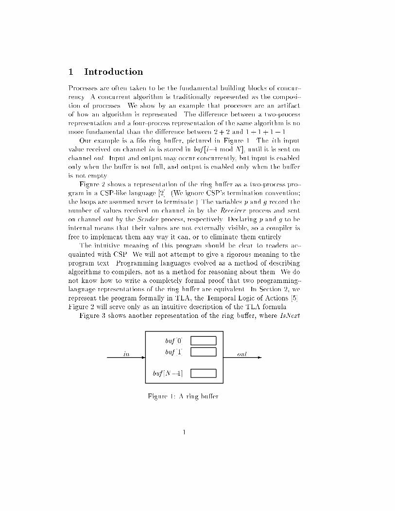
Our example is a �fo ring bu�er, pictured in Figure 1. The ith input
value received on channel in is stored in buf [i�1 mod N ], until it is sent on
channel out . Input and output may occur concurrently, but input is enabled
only when the bu�er is not full, and output is enabled only when the bu�er
is not empty.
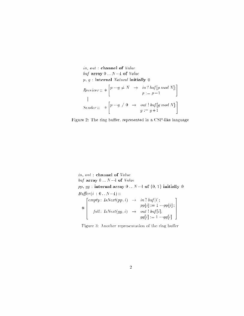
Figure 2 shows a representation of the ring bu�er as a two-process pro-
gram in a CSP-like language [2]. (We ignore CSP's termination convention;
the loops are assumed never to terminate.) The variables p and g record the
number of values received on channel in by the Receiver process and sent
on channel out by the Sender process, respectively. Declaring p and g to be
internal means that their values are not externally visible, so a compiler is
free to implement them any way it can, or to eliminate them entirely.
The intuitive meaning of this program should be clear to readers ac-
quainted with CSP. We will not attempt to give a rigorous meaning to the
program text. Programming languages evolved as a method of describing
algorithms to compilers, not as a method for reasoning about them. We do
not know how to write a completely formal proof that two programming-
language representations of the ring bu�er are equivalent. In Section 2, we
represent the program formally in TLA, the Temporal Logic of Actions [5].
Figure 2 will serve only as an intuitive description of the TLA formula.
Figure 3 shows another representation of the ring bu�er, where IsNext
buf [0]
buf [1]...
buf [N�1]
-in -out
Figure 1: A ring bu�er.
1
in, out : channel of Value
buf array 0 : : N�1 of Value
p, g : internal Natural initially 0
Receiver :: �
"p � g 6= N ! in ? buf [p mod N ];
p := p+1
#jj
Sender :: �
"p � g 6= 0 ! out ! buf [g mod N ];
g := g+1
#
Figure 2: The ring bu�er, represented in a CSP-like language.
in, out : channel of Value
buf array 0 : : N�1 of Value
pp, gg : internal array 0 : : N�1 of f0; 1g initially 0
Bu�er(i : 0 : :N�1) ::
�
26664empty : IsNext(pp; i) ! in ? buf [i ];
pp[i ] := 1� pp[i ] ;
full : IsNext(gg ; i) ! out ! buf [i ];
gg [i ] := 1� gg [i ]
37775Figure 3: Another representation of the ring bu�er.
2

p pp[0] pp[1] pp[2] pp[3]
0 0 0 0 0
1 1 0 0 0
2 1 1 0 0
3 1 1 1 0
4 1 1 1 1
5 0 1 1 1
6 0 0 1 1...
......
......
Figure 4: The correspondence between values of pp and p, for N = 4.
is de�ned by
IsNext(r ; i)�
= if i = 0 then r [0] = r [N�1]else r [i ] 6= r [i�1]
This is as an N -process program; the ith process, Bu�er(i), reads and writes
buf [i ]. Variables p and g of the two-process program are replaced by arrays
pp and gg of bits. Array elements pp[i ] and gg [i ] are read and written by
process Bu�er(i), and are read by process Bu�er(i+1 mod N ).
The two programs are equivalent because the values assumed by pp and
gg in the N -process program correspond directly to the values assumed by
p and g in the two-process one. The correspondence between pp and p is
shown in Figure 4 for N = 4. A boxed number in the pp[i ] column indicates
that IsNext(pp; i) equals true. The correspondence between gg and g is
the same.
It is not hard to argue informally that the two programs are equivalent.
Formalizing this argument should be as straightforward as proving formally
that 222 + 222 equals 111 + 111 + 111 + 111. But, even if straightforward,
a completely formal proof of either result from �rst principles is not trivial.
In Section 3, we sketch a formal TLA proof that the two versions of the ring
bu�er are equivalent.
2 The Algorithm in TLA
We now write the TLA formulas that describe the programs of Figures
2 and 3. The program texts do not tell us what liveness properties are
3
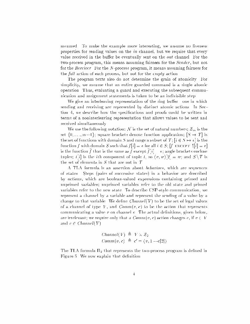
assumed. To make the example more interesting, we assume no liveness
properties for sending values on the in channel, but we require that every
value received in the bu�er be eventually sent on the out channel. For the
two-process program, this means assuming fairness for the Sender , but not
for the Receiver . For the N -process program, it means assuming fairness for
the full action of each process, but not for the empty action.
The program texts also do not determine the grain of atomicity. For
simplicity, we assume that an entire guarded command is a single atomic
operation. Thus, evaluating a guard and executing the subsequent commu-
nication and assignment statements is taken to be an indivisible step.
We give an interleaving representation of the ring bu�er|one in which
sending and receiving are represented by distinct atomic actions. In Sec-
tion 4, we describe how the speci�cations and proofs could be written in
terms of a noninterleaving representation that allows values to be sent and
received simultaneously.
We use the following notation: N is the set of natural numbers; Zm is the
set f0; : : : ;m�1g; square brackets denote function application; [S ! T ] is
the set of functions with domain S and range a subset of T ; [i 2 S 7! e] is the
function f with domain S such that f [i ] = e for all i 2 S ; [f except ! [i ] = e]
is the function bf that is the same as f except bf [i ] = e; angle brackets enclose
tuples; t [i ] is the ith component of tuple t , so hv ;w i[2] = w ; and S nT is
the set of elements in S that are not in T .
A TLA formula is an assertion about behaviors , which are sequences
of states. Steps (pairs of successive states) in a behavior are described
by actions , which are boolean-valued expressions containing primed and
unprimed variables; unprimed variables refer to the old state and primed
variables refer to the new state. To describe CSP-style communication, we
represent a channel by a variable and represent the sending of a value by a
change to that variable. We de�ne Channel(V ) to be the set of legal values
of a channel of type V , and Comm(v ; c) to be the action that represents
communicating a value v on channel c. The actual de�nitions, given below,
are irrelevant; we require only that a Comm(v ; c) action changes c, if v 2 V
and c 2 Channel(V ).
Channel(V )�
= V �Z2
Comm(v ; c)�
= c0 = hv ; 1� c[2]i
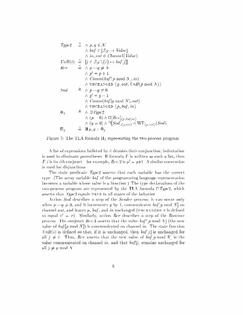
The TLA formula �2 that represents the two-process program is de�ned in
Figure 5. We now explain that de�nition.
4
Type2�
= ^ p; g 2 N
^ buf 2 [ZN ! Value]
^ in; out 2 Channel(Value)
UnB(i)�
= [j 2 ZN nfig 7! buf [j ]]
Rcv�
= ^ p � g 6= N
^ p0 = p + 1
^ Comm(buf 0[p mod N ]; in)
^ unchanged hg ; out ;UnB(p mod N )i
Snd�
= ^ p � g 6= 0
^ g 0 = g + 1
^ Comm(buf [g mod N ]; out)
^ unchanged hp; buf ; in i
�2
�
= ^ 2Type2
^ (p = 0) ^2[Rcv ]hp;buf ;in i
^ (g = 0) ^2[Snd ]hg ;outi ^WFhg;out i(Snd)
�2
�
= 999999 p; g : �2
Figure 5: The TLA formula �2 representing the two-process program.
A list of expressions bulleted by ^ denotes their conjunction; indentation
is used to eliminate parentheses. If formula F is written as such a list, then
F :i is its ith conjunct|for example, Rcv :2 is p0 = p+1. A similar convention
is used for disjunctions.
The state predicate Type2 asserts that each variable has the correct
type. (The array variable buf of the programming language representation
becomes a variable whose value is a function.) The type declarations of the
two-process program are represented by the TLA formula 2Type2, which
asserts that Type2 equals true in all states of the behavior.
Action Snd describes a step of the Sender process; it can occur only
when p � g 6= 0, and it increments g by 1, communicates buf [g mod N ] on
channel out , and leaves p, buf , and in unchanged (unchanged v is de�ned
to equal v 0 = v). Similarly, action Rcv describes a step of the Receiver
process. The conjunct Rcv :3 asserts that the value buf 0[p mod N ] (the new
value of buf [p mod N ]) is communicated on channel in. The state function
UnB(i) is de�ned so that, if it is unchanged, then buf [j ] is unchanged for
all j 6= i . Thus, Rcv asserts that the new value of buf [p mod N ] is the
value communicated on channel in, and that buf [j ] remains unchanged for
all j 6= p mod N .
5

Formula �2:2 describes the Receiver process. It asserts that p is initially
0, and that every step is a Rcv step or leaves p, buf , and in unchanged ([A]vis de�ned to equal A_ (v 0 = v)). Steps that leave p, buf , and in unchanged
represent steps of the Receiver 's environment|either steps of the Sender
or steps of the entire program's environment. The conjunct �2:3 similarly
represents the Sender process. The formula WFhg;out i(Snd) asserts weak
fairness of the Snd action. In general, WFv (A) asserts that if action hAiv(de�ned to equal A^ (v 0 6= v)) remains continuously enabled, then an hAivstep must eventually occur.
Formula �2 is the conjunction of the speci�cations of the two processes
with the formula asserting type correctness. It describes the two-process
program with p and g visible. The complete program speci�cation �2 is
obtained by hiding p and g . In logic, hiding means existential quanti�cation;
in temporal logic, exible variables (distinct from rigid variables like N ) are
hidden with the temporal existential quanti�er 999999 .The conjunct 2Type2 of �2 makes type correctness an explicit part of
the speci�cation. We put type-correctness assumptions in our speci�cations
to make them as much like Figures 2 and 3 as possible. However, to avoid
errors, it is usually better to let type correctness be a consequence of the
speci�cation. We could rewrite �2 as follows to eliminate the conjunct
2Type2. The conjunct 2Type2:1 is already redundant because it is implied
by �2:2 ^ �2:3. We can eliminate 2Type2:3 by making Type2:3 part of
the initial condition, since Type2:3 ^ �2:2 ^ �2:3 implies 2Type2:3. (The
proof requires the fact that c 2 Channel(V ) and Comm(v ; c) imply c0 2Channel(V ).) We can eliminate 2Type2:2 in the same way, if we modify
Rcv so it leaves the domain of buf unchanged.
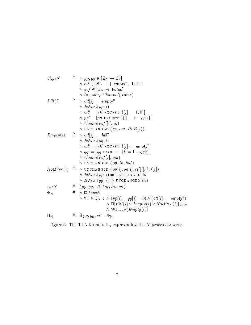
The TLA formula �N that represents the N -process program is de�ned
in Figure 6. There are two things in this de�nition that merit further ex-
planation. First, we introduce an array ctl to represent the control state.
The value of ctl [i ] equals \empty" if control in process Bu�er(i) is at the
point labeled empty , and it equals \full" if control is at full . Second, we
introduce an action NotProc(i) that has no obvious counterpart in Figure 3
or in �2. The speci�cations of the two processes in Figure 2 are especially
simple because each variable is changed by an action of only one of the
processes. For example, a step of the Sender 's environment can be char-
acterized as any step that leaves g and out unchanged. We can think of
g and out as belonging to the Sender . In the N -process program, pp[i ],
gg [i ], and ctl [i ] belong to Bu�er(i). However, in and out don't belong to
any single process; they can be changed by a step of any of the N pro-
6
TypeN�
= ^ pp; gg 2 [ZN ! Z2]^ ctl 2 [ZN ! f\empty"; \full"g]
^ buf 2 [ZN ! Value]
^ in; out 2 Channel(Value)
Fill(i)�
= ^ ctl [i ] = \empty"
^ IsNext(pp; i)
^ ctl 0 = [ctl except ! [i ] = \full"]
^ pp0 = [pp except ! [i ] = 1� pp[i ]]
^ Comm(buf 0[i ]; in)
^ unchanged hgg ; out ;UnB(i)i
Empty(i)�
= ^ ctl [i ] = \full"
^ IsNext(gg ; i)
^ ctl 0 = [ctl except ! [i ] = \empty"]
^ gg 0 = [gg except ! [i ] = 1� gg [i ]]
^ Comm(buf [i ]; out)
^ unchanged hpp; in; buf i
NotProc(i)�
= ^ unchanged hpp[i ]; gg [i ]; ctl [i ]; buf [i ]i^ IsNext(pp; i)) unchanged in
^ IsNext(gg ; i)) unchanged out
varN�
= hpp; gg ; ctl ; buf ; in; out i
�N
�
= ^ 2TypeN^ 8 i 2 ZN : ^ (pp[i ] = gg [i ] = 0) ^ (ctl [i ] = \empty")
^ 2[Fill(i)_ Empty(i)_NotProc(i)]varN^ WFvarN (Empty(i))
�N
�
= 999999 pp; gg ; ctl : �N
Figure 6: The TLA formula �N representing the N -process program.
7

cesses. The variable in belongs to Bu�er(i) only when IsNext(pp; i) equals
true, and out belongs to Bu�er(i) only when IsNext(gg ; i) equals true.
Action NotProc(i) characterizes steps of Bu�er(i)'s environment, which is
allowed to change in when IsNext(pp; i) equals false, and to change out
when IsNext(gg ; i) equals false. The subscript in 2[: : :]varN allows steps of
the entire program's environment that leave all the variables unchanged. It
is semantically super uous, since NotProc(i) already allows such steps, but
the syntax of TLA requires some subscript.
3 The Proof
We now give a hierarchically structured proof that �2 and �N are equiva-
lent [4]. The proof is completely formal, meaning that each step is a mathe-
matical formula. English is used only to explain the low-level reasoning. The
entire proof could be carried down to a level at which each step follows from
the simple application of formal rules, but such a detailed proof is more suit-
able for machine checking than human reading. Our complete proof, with
\Q.E.D." steps and low-level reasoning omitted, appears in Appendix A.
The correctness of the algorithm rests on simple properties of integers
and of the mod operator. We need the following lemma, where the bit array
Rep(m) used to represent the integer m is de�ned by
Rep(m)�
= [i 2 ZN 7! if i < m mod 2N � i +N then 1 else 0]
The lemma is proved in Appendix B. We assume throughout that N is a
positive integer.
Lemma 1 If m 2 N and i 2 ZN , then
1. IsNext(Rep(m); i)� (i = m mod N )
2. IsNext(Rep(m); i))
Rep(m + 1) = [Rep(m) except ! [i ] = 1� Rep(m)[i ]]
For temporal reasoning, we use the following TLA rules from Figure 5 of [5].
8
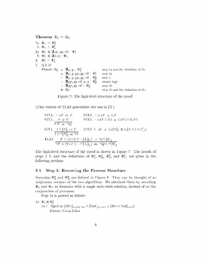
Theorem �2 � �N
1a. �2 � �u
2
b. �N � �u
N
2a. �u
2� 999999pp; gg ; ctl : �h
2
b. �u
N� 999999p; g : �h
N
3. �h
2� �h
N
4. Q.E.D.
Proof: �2 � 999999 p; g : �u
2step 1a and the de�nition of �2
� 999999 p; g ; pp; gg ; ctl : �h
2step 2a
� 999999 p; g ; pp; gg ; ctl : �h
Nstep 3
� 999999 pp; gg ; ctl ; p; g : �h
Nsimple logic
� 999999 pp; gg ; ctl : �u
Nstep 2b
� �N step 1b and the de�nition of �N
Figure 7: The high-level structure of the proof.
(This version of TLA2 generalizes the one in [5].)
STL2: ` 2F ) F STL3: ` 22F � 2F
STL4: F ) G
2F ) 2G
STL5: ` 2(F ^G) � (2F ) ^ (2G)
INV1: I ^ [N ]f ) I0
I ^2[N ]f ) 2I
INV2: ` 2I ) (2[N ]f � 2[N ^ I ^ I0]f )
TLA2: P ^ (8 i 2 S : [Ai ]fi ) ) Q ^ [B ]g
2P ^ (8 i 2 S : 2[Ai ]fi ) ) 2Q ^2[B ]g
The high-level structure of the proof is shown in Figure 7. The proofs of
steps 1{3, and the de�nitions of �u2 , �
u
N, �h
2, and �h
N, are given in the
following sections.
3.1 Step 1: Removing the Process Structure
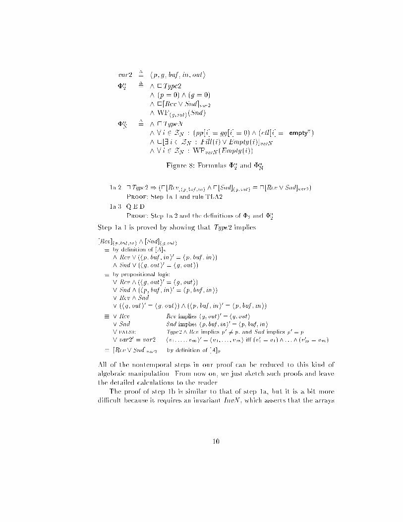
Formulas �u2 and �u
Nare de�ned in Figure 8. They can be thought of as
uniprocess versions of the two algorithms. We obtained them by rewriting
�2 and �N as formulas with a single next-state relation, instead of as the
conjunction of processes.
Step 1a is proved as follows.
1a. �2 � �u
2
1a.1. Type2) ([Rcv ]hp;buf ;in i ^ [Snd ]hg;out i � [Rcv _ Snd ]var2)
Proof: Given below.
9
var2�
= hp; g ; buf ; in; out i
�u2
�
= ^ 2Type2^ (p = 0) ^ (g = 0)
^ 2[Rcv _ Snd ]var2^ WFhg;out i(Snd)
�u
N
�
= ^ 2TypeN^ 8 i 2 ZN : (pp[i ] = gg [i ] = 0)^ (ctl [i ] = \empty")
^ 2[9 i 2 ZN : Fill(i)_ Empty(i)]varN^ 8 i 2 ZN : WFvarN (Empty(i))
Figure 8: Formulas �u2and �u
N.
1a.2. 2Type2) (2[Rcv ]hp;buf ;in i ^2[Snd ]hg;out i � 2[Rcv _ Snd ]var2)
Proof: Step 1a.1 and rule TLA2.
1a.3. Q.E.D.
Proof: Step 1a.2 and the de�nitions of �2 and �u
2.
Step 1a.1 is proved by showing that Type2 implies
[Rcv ]hp;buf ;in i ^ [Snd ]hg;out i
� by de�nition of [A]v
^ Rcv _ (hp; buf ; in i0 = hp; buf ; in i)
^ Snd _ (hg ; out i0 = hg ; out i)
� by propositional logic
_ Rcv ^ (hg ; out i0 = hg ; out i)
_ Snd ^ (hp; buf ; in i0 = hp; buf ; in i)
_ Rcv ^ Snd
_ (hg ; out i0 = hg ; out i) ^ (hp; buf ; in i0 = hp; buf ; in i)
� _ Rcv Rcv implies hg;out i0 = hg;out i
_ Snd Snd implies hp; buf ; in i0 = hp; buf ; in i
_ false Type2 ^Rcv implies p0 6= p, and Snd implies p0= p
_ var20 = var2 hv1; : : : ; vm i0 = hv1; : : : ; vm i i� (v 0
1 = v1) ^ : : : ^ (v 0
m = vm)
� [Rcv _ Snd ]var2 by de�nition of [A]v
All of the nontemporal steps in our proof can be reduced to this kind of
algebraic manipulation. From now on, we just sketch such proofs and leave
the detailed calculations to the reader.
The proof of step 1b is similar to that of step 1a, but it is a bit more
di�cult because it requires an invariant InvN , which asserts that the arrays
10
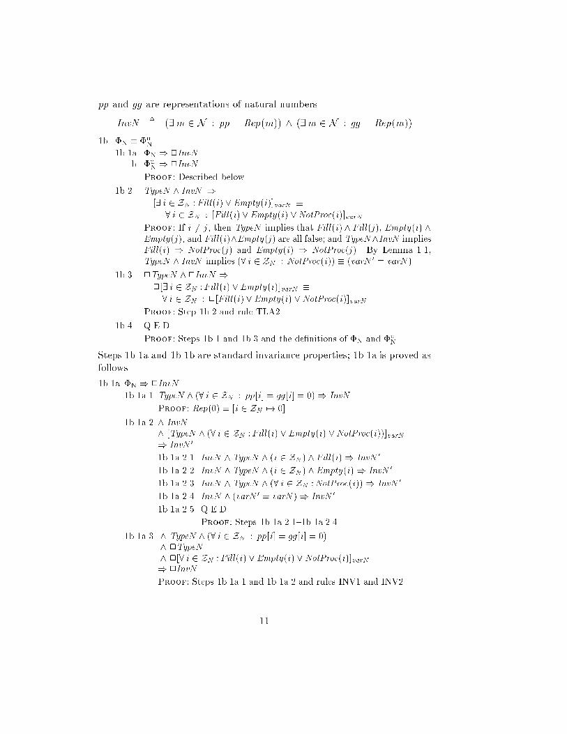
pp and gg are representations of natural numbers.
InvN�
= (9m 2 N : pp = Rep(m)) ^ (9m 2 N : gg = Rep(m))
1b. �N � �u
N
1b.1a. �N ) 2InvN
b. �u
N) 2InvN
Proof: Described below.
1b.2. TypeN ^ InvN )
[9 i 2 ZN :Fill(i) _ Empty(i)]varN �
8 i 2 ZN : [Fill(i)_ Empty(i) _NotProc(i)]varN
Proof: If i 6= j , then TypeN implies that Fill(i)^ Fill(j ), Empty(i) ^
Empty(j ), and Fill(i)^Empty(j ) are all false; and TypeN^InvN implies
Fill(i) ) NotProc(j ) and Empty(i) ) NotProc(j ). By Lemma 1.1,
TypeN ^ InvN implies (8 i 2 ZN : NotProc(i)) � (varN 0 = varN ).
1b.3. 2TypeN ^2InvN )
2[9 i 2 ZN :Fill(i) _ Empty(i)]varN �
8 i 2 ZN : 2[Fill(i)_ Empty(i) _NotProc(i)]varN
Proof: Step 1b.2 and rule TLA2.
1b.4 Q.E.D.
Proof: Steps 1b.1 and 1b.3 and the de�nitions of �N and �u
N.
Steps 1b.1a and 1b.1b are standard invariance properties; 1b.1a is proved as
follows.
1b.1a �N ) 2InvN
1b.1a.1 TypeN ^ (8 i 2 ZN : pp[i ] = gg [i ] = 0)) InvN
Proof: Rep(0) = [i 2 ZN 7! 0]
1b.1a.2 ^ InvN
^ [TypeN ^ (8 i 2 ZN :Fill(i) _ Empty(i) _NotProc(i))]varN) InvN
0
1b.1a.2.1. InvN ^TypeN ^ (i 2 ZN ) ^ Fill(i)) InvN0
1b.1a.2.2. InvN ^TypeN ^ (i 2 ZN ) ^ Empty(i)) InvN0
1b.1a.2.3. InvN ^TypeN ^ (8 i 2 ZN :NotProc(i))) InvN0
1b.1a.2.4. InvN ^ (varN 0 = varN )) InvN0
1b.1a.2.5. Q.E.D.
Proof: Steps 1b.1a.2.1{1b.1a.2.4.
1b.1a.3. ^ TypeN ^ (8 i 2 ZN : pp[i ] = gg [i ] = 0)
^ 2TypeN
^ 2[8 i 2 ZN :Fill(i) _ Empty(i) _NotProc(i)]varN) 2InvN
Proof: Steps 1b.1a.1 and 1b.1a.2 and rules INV1 and INV2.
11

1b.1a.4. Q.E.D.
Proof: Step 1b.1a.3 and rule TLA2, since (8 i : [Ai ]v) � [8 i :Ai ]v .
Steps 1b.1a.2.1 and 1b.1a.2.2 are proved using Lemma 1.2; steps 1b.1a.2.3
and 1b.1a.2.4 follow because their hypotheses imply pp 0 = pp and gg 0 = gg .
As indicated in the appendix, the proof of step 1b.1b is similar.
3.2 Step 2: Adding History Variables
Formulas �h2and �h
Nare de�ned in Figure 9, which also de�nes their safety
parts, �hS2 and �hS
N. We obtained �h
2 by adding pp, gg , and ctl as history
variables to �u2; and we obtained �h
Nby adding p and g as history variables
to �u
N. In general, adding an auxiliary variable a to a formula F means
writing a formula F a such that F � 999999 a : F a . A history variable is an
auxiliary variable that records information from previous states. It is added
by using the following lemma, which can be deduced from the results in [1].
Step 2 is easily proved by repeated application of this lemma.
Lemma 2 (History Variable) If h and h0 do not occur in Init, Ai , Bj ,
v , or f, and h0 does not occur in g i , for all i 2 I and j 2 J , then
Init ^ 2[9 i 2 I : Ai ]v ^ (8 j 2 J : WFv (Bj ))
� 999999 h : ^ Init ^ (h = f )
^ 2[9 i 2 I : Ai ^ (h 0 = g i)]hh;v i
^ 8 j 2 J : WFv (Bj )
3.3 Step 3: Equivalence of �h
2and �h
N
In the two-process algorithm, p and g are the actual internal variables, while
pp, gg , and ctl are history variables. The situation is reversed in the N -
process algorithm. Step 3 involves showing that the history variables of one
algorithm behave like the internal variables of the other. Its proof uses the
following formulas, where Inv will be shown to be an invariant of both �h2
and �h
N.
IsFull(g ; p; i)�
= 9m 2 N : (g � m < p)^ (i = m mod N )
Inv�
= ^ pp = Rep(p)
^ gg = Rep(g)
^ ctl = [i 2 ZN 7! if IsFull(g ; p; i) then \full" else \empty"]
^ 0 � p � g � N
The high-level structure of the proof is:
12
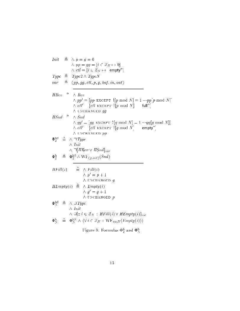
Init�
= ^ p = g = 0
^ pp = gg = [i 2 ZN 7! 0]
^ ctl = [i 2 ZN 7! \empty"]
Type�
= Type2 ^ TypeN
var�
= hpp; gg ; ctl ; p; g ; buf ; in; out i
HRcv�
= ^ Rcv
^ pp0 = [pp except ! [p mod N ] = 1� pp[p mod N ]]
^ ctl 0 = [ctl except ! [p mod N ] = \full"]
^ unchanged gg
HSnd�
= ^ Snd
^ gg 0 = [gg except ! [g mod N ] = 1� gg [g mod N ]]
^ ctl 0 = [ctl except ! [g mod N ] = \empty"]
^ unchanged pp
�hS2
�
= ^ 2Type^ Init
^ 2[HRcv _ HSnd ]var
�h2
�
= �hS2^WFhg;out i(Snd)
HFill(i)�
= ^ Fill(i)
^ p0 = p + 1
^ unchanged g
HEmpty(i)�
= ^ Empty(i)
^ g 0 = g + 1
^ unchanged p
�hS
N
�
= ^ 2Type
^ Init
^ 2[9 i 2 ZN : HFill(i)_ HEmpty(i)]var
�h
N
�
= �hS
N^ (8 i 2 ZN : WFvarN (Empty(i)))
Figure 9: Formulas �h2and �h
N.
13
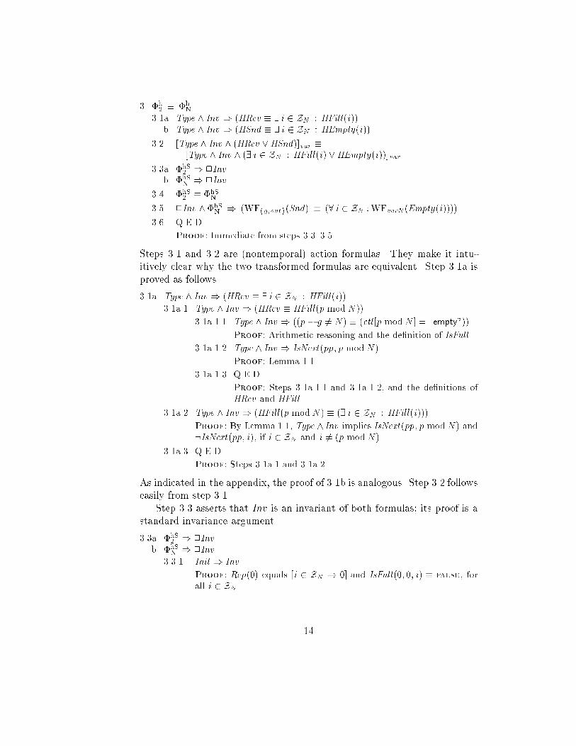
3. �h
2� �h
N
3.1a. Type ^ Inv ) (HRcv � 9 i 2 ZN : HFill(i))
b. Type ^ Inv ) (HSnd � 9 i 2 ZN : HEmpty(i))
3.2. [Type ^ Inv ^ (HRcv _HSnd)]var �
[Type ^ Inv ^ (9 i 2 ZN : HFill(i) _HEmpty(i))]var
3.3a. �hS
2) 2Inv
b. �hS
N) 2Inv
3.4. �hS
2� �hS
N
3.5. 2Inv ^�hS
N) (WFhg;out i(Snd) � (8 i 2 ZN :WFvarN (Empty(i))))
3.6. Q.E.D.
Proof: Immediate from steps 3.3{3.5.
Steps 3.1 and 3.2 are (nontemporal) action formulas. They make it intu-
itively clear why the two transformed formulas are equivalent. Step 3.1a is
proved as follows.
3.1a. Type ^ Inv ) (HRcv � 9 i 2 ZN : HFill(i))
3.1a.1 Type ^ Inv ) (HRcv � HFill(p mod N ))
3.1a.1.1. Type ^ Inv ) ((p � g 6= N ) � (ctl [p mod N ] = \empty"))
Proof: Arithmetic reasoning and the de�nition of IsFull .
3.1a.1.2. Type ^ Inv ) IsNext(pp; p mod N )
Proof: Lemma 1.1.
3.1a.1.3. Q.E.D.
Proof: Steps 3.1a.1.1 and 3.1a.1.2, and the de�nitions of
HRcv and HFill .
3.1a.2 Type ^ Inv ) (HFill(p mod N ) � (9 i 2 ZN : HFill(i)))
Proof: By Lemma 1.1, Type ^ Inv implies IsNext(pp; p mod N ) and
:IsNext(pp; i), if i 2 ZN and i 6= (p mod N ).
3.1a.3 Q.E.D.
Proof: Steps 3.1a.1 and 3.1a.2.
As indicated in the appendix, the proof of 3.1b is analogous. Step 3.2 follows
easily from step 3.1.
Step 3.3 asserts that Inv is an invariant of both formulas; its proof is a
standard invariance argument.
3.3a. �hS
2) 2Inv
b. �hS
N) 2Inv
3.3.1. Init ) Inv
Proof: Rep(0) equals [i 2 ZN 7! 0] and IsFull(0; 0; i) � false, for
all i 2 ZN .
14
3.3.2a. Inv ^ [Type ^ (HRcv _HSnd)]var ) Inv0
b. Inv ^ [Type ^ (9 i 2 ZN : HFill(i) _HEmpty(i))]var ) Inv0
Proof: Given below.
3.3.3. Q.E.D.
Proof: Steps 3.3.1 and 3.3.2, and rules INV1 and INV2.
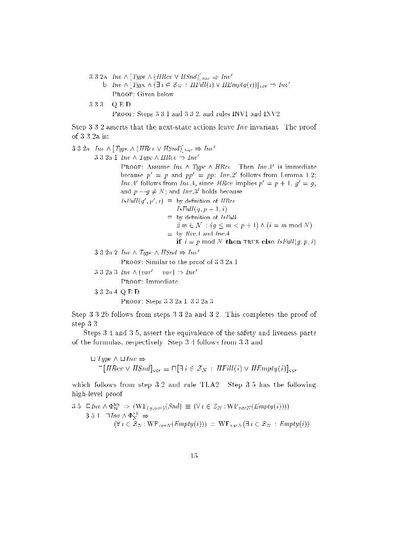
Step 3.3.2 asserts that the next-state actions leave Inv invariant. The proof
of 3.3.2a is:
3.3.2a. Inv ^ [Type ^ (HRcv _HSnd)]var ) Inv0
3.3.2a.1 Inv ^Type ^HRcv ) Inv0
Proof: Assume Inv ^ Type ^ HRcv . Then Inv :10 is immediate
because p0 = p and pp
0 = pp; Inv :20 follows from Lemma 1.2;
Inv :40 follows from Inv :4, since HRcv implies p0 = p + 1, g 0 = g ,
and p � g 6= N ; and Inv :30 holds because
IsFull(g 0; p
0; i) � by de�nition of HRcv
IsFull(g ; p + 1; i)
� by de�nition of IsFull
9m 2 N : (g � m < p + 1) ^ (i = m mod N )
� by Rcv :1 and Inv :4
if i = p mod N then true else IsFull(g ; p; i)
3.3.2a.2 Inv ^Type ^HSnd ) Inv0
Proof: Similar to the proof of 3.3.2a.1.
3.3.2a.3 Inv ^ (var 0 = var)) Inv0
Proof: Immediate.
3.3.2a.4 Q.E.D.
Proof: Steps 3.3.2a.1{3.3.2a.3.
Step 3.3.2b follows from steps 3.3.2a and 3.2. This completes the proof of
step 3.3.
Steps 3.4 and 3.5, assert the equivalence of the safety and liveness parts
of the formulas, respectively. Step 3.4 follows from 3.3 and
2Type ^ 2Inv )
2[HRcv _ HSnd ]var � 2[9 i 2 ZN : HFill(i)_HEmpty(i)]var
which follows from step 3.2 and rule TLA2. Step 3.5 has the following
high-level proof.
3.5. 2Inv ^�hS
N) (WFhg;out i(Snd) � (8 i 2 ZN :WFvarN (Empty(i))))
3.5.1. 2Inv ^ �hS
N)
(8 i 2 ZN :WFvarN (Empty(i))) � WFvarN (9 i 2 ZN : Empty(i))
15

3.5.2. 2Inv ^2Type ^2[HRcv _HSnd ]var )
WFhg;out i(Snd) � WFvarN (9 i 2 ZN :Empty(i))
3.5.3. Q.E.D.
Proof: Steps 3.5.1 and 3.5.2.
We �rst consider step 3.5.1. When writing TLA speci�cations, one often has
to choose between asserting fairness of A1 _ : : :_Am and asserting fairness
of each action Ai . The choice becomes a matter of taste when the resulting
speci�cations are equivalent. This is the case if, whenever one of the Ai
becomes enabled, a step of no other Aj can occur before the next Ai step.
For weak fairness, the equivalence is a consequence of the following result,
which can be derived from the TLA proof rules of [5].
Lemma 3 If
Enabled hAi iv ^ 2Inv ^ 2[N ^ :Ai ]v ) 2:Enabled hAj iv
for all i ; j 2 S with i 6= j , then
2Inv ^ 2[N ]v ) (WFv (9 i 2 S : Ai ) � (8 i 2 S : WFv (Ai )))
We use this lemma to prove step 3.5.1.
3.5.1. 2Inv ^ �hS
N)
(8 i 2 ZN :WFvarN (Empty(i))) �WFvarN (9 i 2 ZN :Empty(i)))
3.5.1.1. �hS
N) 2[9 i 2 ZN : Fill(i) _ Empty(i)]varN
Proof: TLA2, since HFill(i)) Fill(i) and HEmpty(i)) Empty(i).
3.5.1.2. ^ i 2 ZN
^ IsNext(gg ; i)
^ 2(Inv ^Type)
^ 2[(9 j 2 ZN : Fill(j ) _ Empty(j )) ^ :Empty(i)]varN) 2IsNext(gg ; i)
Proof: By rules INV1 and INV2, since
Inv ^Type ^ (Fill(j ) _ Empty(j )) ^ :Empty(i)
implies gg 0 = gg , for all i ; j 2 ZN .
3.5.1.3. ^ (i ; j 2 ZN ) ^ (i 6= j )
^ Enabled hEmpty(i)ivarN^ 2(Inv ^Type)
^ 2[(9 k 2 ZN : Fill(k) _Empty(k)) ^ :Empty(i)]varN) 2:Enabled hEmpty(j )ivarN
Proof: Step 3.5.1.2 and rule STL4, since Enabled hEmpty(i)ivarNimplies IsNext(gg ; i), and Lemma 1.1 implies
Inv ^Type ^ IsNext(gg ; i)) :IsNext(gg ; j )
for all i ; j 2 ZN with i 6= j .
16
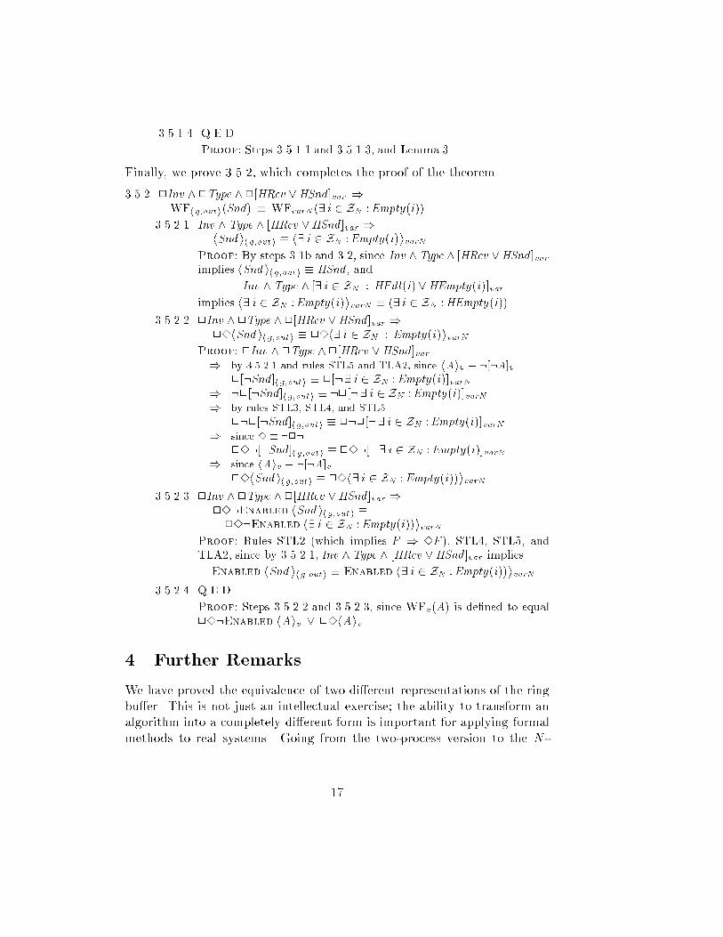
3.5.1.4. Q.E.D.
Proof: Steps 3.5.1.1 and 3.5.1.3, and Lemma 3.
Finally, we prove 3.5.2, which completes the proof of the theorem.
3.5.2. 2Inv ^2Type ^2[HRcv _HSnd ]var )
WFhg;out i(Snd) � WFvarN (9 i 2 ZN :Empty(i))
3.5.2.1. Inv ^ Type ^ [HRcv _HSnd ]var )
hSnd ihg;out i � h9 i 2 ZN :Empty(i)ivarN
Proof: By steps 3.1b and 3.2, since Inv ^Type ^ [HRcv _HSnd ]varimplies hSnd ihg;out i � HSnd , and
Inv ^Type ^ [9 i 2 ZN : HFill(i)_HEmpty(i)]var
implies h9 i 2 ZN :Empty(i)ivarN � (9 i 2 ZN :HEmpty(i)).
3.5.2.2. 2Inv ^2Type ^2[HRcv _HSnd ]var )
23hSnd ihg;out i � 23h9 i 2 ZN : Empty(i)ivarN
Proof: 2Inv ^2Type ^2[HRcv _HSnd ]var) by 3.5.2.1 and rules STL5 and TLA2, since hAiv � :[:A]v
2[:Snd ]hg;out i � 2[:9 i 2 ZN :Empty(i)]varN) :2[:Snd ]hg;out i � :2[:9 i 2 ZN :Empty(i)]varN) by rules STL3, STL4, and STL5
2:2[:Snd ]hg;out i � 2:2[:9 i 2 ZN :Empty(i)]varN) since 3� :2:
23:[:Snd ]hg;out i � 23:[:9 i 2 ZN :Empty(i)]varN) since hAiv � :[:A]v
23hSnd ihg;out i � 23h9 i 2 ZN :Empty(i))ivarN
3.5.2.3 2Inv ^2Type ^2[HRcv _HSnd ]var )
23:Enabled hSnd ihg;out i �
23:Enabled h9 i 2 ZN :Empty(i))ivarN
Proof: Rules STL2 (which implies F ) 3F ), STL4, STL5, and
TLA2, since by 3.5.2.1, Inv ^Type ^ [HRcv _HSnd ]var implies
Enabled hSnd ihg;out i � Enabled h9 i 2 ZN :Empty(i))ivarN
3.5.2.4 Q.E.D.
Proof: Steps 3.5.2.2 and 3.5.2.3, since WFv (A) is de�ned to equal
23:Enabled hAiv _ 23hAiv .
4 Further Remarks
We have proved the equivalence of two di�erent representations of the ring
bu�er. This is not just an intellectual exercise; the ability to transform an
algorithm into a completely di�erent form is important for applying formal
methods to real systems. Going from the two-process version to the N -
17

process one reduces the internal state of each process from an unbounded
number (p or g) to three bits (pp[i ], gg [i ], and ctl [i ]). As explained in [3],
such a transformation enables us to apply model checking to unbounded-
state systems.
In retrospect, it is not surprising that programs with di�erent numbers
of processes can be equivalent. Multiprocess programs are routinely exe-
cuted on single-processor computers by interleaving the execution of their
processes. The transformation of �2 and �N to �u2 and �u
Ncan be viewed
as a formal description of this interleaving.
Using an interleaving representation makes the proof of equivalence a
bit simpler, but it is not necessary. The equivalence of noninterleaving
representations can be proved as follows. Let RcvNI and SndNI be the ac-
tions obtained from Rcv and Snd by removing the unchanged conjuncts
and adding the conjunct unchangedUnB(p mod N ) to RcvNI . Replac-
ing Rcv and Snd with RcvNI and SndNI in the de�nition of �2 yields a
noninterleaving representation of the two-process program. Similarly, we
get a noninterleaving representation of the N -process program by replacing
Fill(i) and Empty(i) with actions FillNI (i) and EmptyNi(i) that have no
unchanged conjuncts except the one for UnB(i). In the proof of equiva-
lence, formula �u2is changed by replacing its next-state action Rcv _ Snd
with Rcv_Snd _(RcvNI ^SndNI ), and �u
Nis changed by replacing its next-
state action with 9 i 2 ZN : Fill(i)_Empty(i)_ (FillNI (i)^EmptyNI (i)).
Formulas �h2 and �h
Nare obtained by adding history variables to the new
versions of �u
2and �u
N. The proof of equivalence is the same as before,
except we have to consider the next-state actions' extra disjuncts. These
disjuncts represent the simultaneous sending and receiving of values.
Indivisible state changes are an abstraction; executing an operation of a
real program takes time. In TLA, we can represent the concurrent execution
of program operations either as successive steps, or as a single step. Which
representation we choose is a matter of convenience, not philosophy. We
have found that interleaving representations are usually, but not always,
more convenient than noninterleaving ones for reasoning about algorithms.
A proof that two algorithms are equivalent can be turned into a deriva-
tion of one algorithm from the other. Our proof yields the following deriva-
tion, where each equivalence is obtained from the indicated proof step(s).
�2 � 999999 : p; g : �u2
1a
� 999999 p; g ; pp; gg ; ctl : �h2 2a
18

� 999999 p; g ; pp; gg ; ctl : �h2 ^2Inv 3.3a
� 999999 pp; gg ; ctl ; p; g : �h
N^2Inv 3.4 and 3.5
� 999999 pp; gg ; ctl ; p; g : �h
N3.3b
� 999999 p; g : �u
N2b
� 999999 p; g : �u
N^2InvN 1b.1b
� 999999 p; g : �N ^2InvN 1b.3
� �N 1b.1a
Our derivation uses rules of logic to rewrite formulas. In process algebra [6],
analogous transformations are performed by applying algebraic laws. It
would be interesting to compare a process-algebraic proof of equivalence of
the two ring-bu�er programs with our TLA proof.
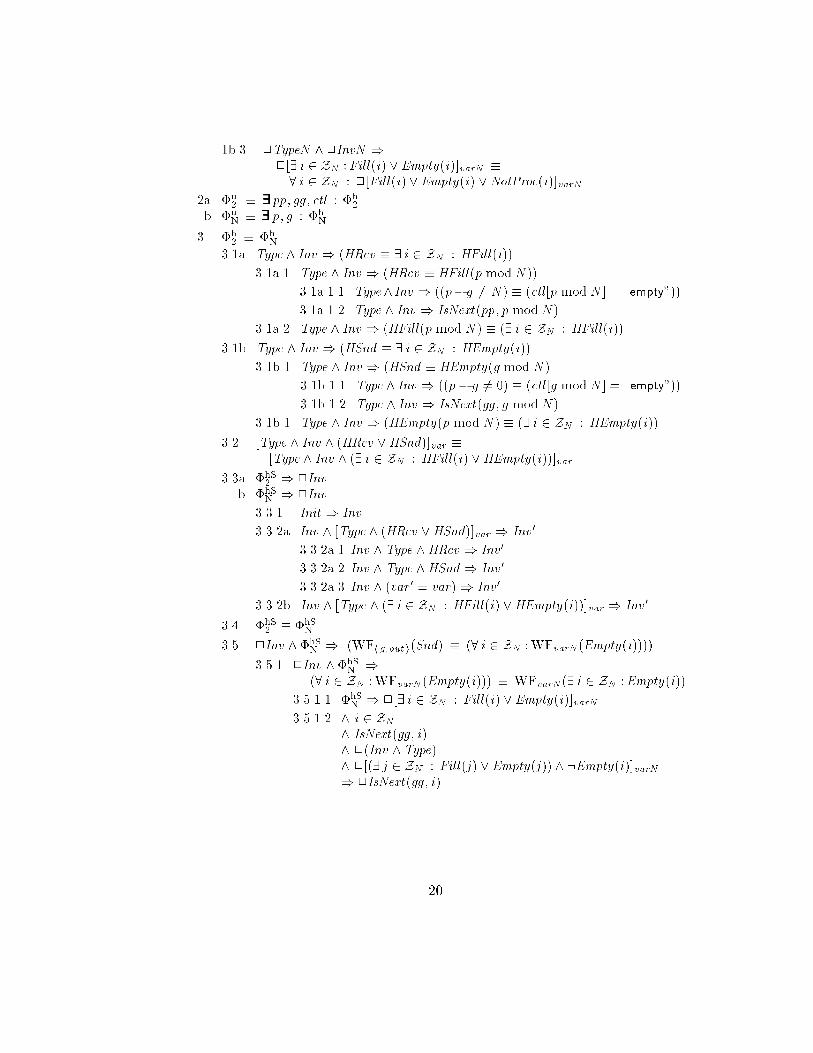
A Proof of the Theorem
Theorem �2 � �N
1a. �2 � �u
2
1a.1. Type2) ([Rcv ]hp;buf ;in i ^ [Snd ]hg;out i � [Rcv _ Snd ]var2)
1a.2. 2Type2) (2[Rcv ]hp;buf ;in i ^2[Snd ]hg;out i � 2[Rcv _ Snd ]var2)
1b. �N � �u
N
1b.1a. �N ) 2InvN
1b.1a.1 TypeN ^ (8 i 2 ZN : pp[i ] = gg [i ] = 0)) InvN
1b.1a.2 ^ InvN
^ [TypeN ^ (8 i 2 ZN :Fill(i) _ Empty(i) _NotProc(i))]varN) InvN
0
1b.1a.3. ^ TypeN ^ (8 i 2 ZN : pp[i ] = gg [i ] = 0)
^ 2TypeN ^2[8 i 2 ZN :Fill(i) _ Empty(i) _NotProc(i)]varN) 2InvN
1b.1b. �u
N) 2InvN
1b.1b.1. TypeN ^ (8 i 2 ZN : pp[i ] = gg [i ] = 0)) InvN
1b.1b.2. ^ InvN
^ [TypeN ^ (9 i 2 ZN : Fill(i)_ Empty(i)]varN) InvN
0
1b.1b.3. ^ TypeN ^ (8 i 2 ZN : pp[i ] = gg [i ] = 0)
^ 2TypeN ^2[9 i 2 ZNFill(i) _ Empty(i)]varN) InvN
0
1b.2. TypeN ^ InvN )
[9 i 2 ZN :Fill(i) _ Empty(i)]varN �
8 i 2 ZN : [Fill(i)_ Empty(i) _NotProc(i)]varN
19
1b.3. 2TypeN ^2InvN )
2[9 i 2 ZN :Fill(i) _ Empty(i)]varN �
8 i 2 ZN : 2[Fill(i)_ Empty(i) _NotProc(i)]varN
2a. �u
2� 999999pp; gg ; ctl : �h
2
b. �u
N� 999999p; g : �h
N
3. �h
2� �h
N
3.1a. Type ^ Inv ) (HRcv � 9 i 2 ZN : HFill(i))
3.1a.1 Type ^ Inv ) (HRcv � HFill(p mod N ))
3.1a.1.1. Type^ Inv ) ((p�g 6= N ) � (ctl [p mod N ] = \empty"))
3.1a.1.2. Type ^ Inv ) IsNext(pp; p mod N )
3.1a.2 Type ^ Inv ) (HFill(p mod N ) � (9 i 2 ZN : HFill(i))
3.1b. Type ^ Inv ) (HSnd � 9 i 2 ZN : HEmpty(i))
3.1b.1 Type ^ Inv ) (HSnd � HEmpty(g mod N )
3.1b.1.1. Type ^ Inv ) ((p � g 6= 0) � (ctl [g mod N ] = \empty"))
3.1b.1.2. Type ^ Inv ) IsNext(gg ; g mod N )
3.1b.1 Type ^ Inv ) (HEmpty(p mod N ) � (9 i 2 ZN : HEmpty(i))
3.2. [Type ^ Inv ^ (HRcv _HSnd)]var �
[Type ^ Inv ^ (9 i 2 ZN : HFill(i) _HEmpty(i))]var
3.3a. �hS
2) 2Inv
b. �hS
N) 2Inv
3.3.1. Init ) Inv
3.3.2a. Inv ^ [Type ^ (HRcv _HSnd)]var ) Inv0
3.3.2a.1 Inv ^Type ^HRcv ) Inv0
3.3.2a.2 Inv ^Type ^HSnd ) Inv0
3.3.2a.3 Inv ^ (var 0 = var)) Inv0
3.3.2b. Inv ^ [Type ^ (9 i 2 ZN : HFill(i) _HEmpty(i))]var ) Inv0
3.4. �hS
2� �hS
N
3.5. 2Inv ^�hS
N) (WFhg;out i(Snd) � (8 i 2 ZN :WFvarN (Empty(i))))
3.5.1. 2Inv ^ �hS
N)
(8 i 2 ZN :WFvarN (Empty(i))) � WFvarN (9 i 2 ZN :Empty(i))
3.5.1.1. �hS
N) 2[9 i 2 ZN : Fill(i) _ Empty(i)]varN
3.5.1.2. ^ i 2 ZN
^ IsNext(gg ; i)
^ 2(Inv ^Type)
^ 2[(9 j 2 ZN : Fill(j ) _ Empty(j )) ^ :Empty(i)]varN) 2IsNext(gg ; i)
20

3.5.1.3. ^ (i ; j 2 ZN ) ^ (i 6= j )
^ Enabled hEmpty(i)ivarN^ 2(Inv ^Type)
^ 2[(9 k 2 ZN : Fill(k) _ Empty(k)) ^ :Empty(i)]varN) 2:Enabled hEmpty(j )ivarN
3.5.2. 2Inv ^2Type ^2[HRcv _HSnd ]var )
WFhg;out i(Snd) � WFvarN (9 i 2 ZN : Empty(i))
3.5.2.1. Inv ^Type ^ [HRcv _HSnd ]var )
hSnd ihg;out i � h9 i 2 ZN :Empty(i)ivarN
3.5.2.2. 2Inv ^2Type ^2[HRcv _HSnd ]var )
23hSnd ihg;out i � 23h9 i 2 ZN : Empty(i))ivarN
3.5.2.3 2Inv ^2Type ^2[HRcv _HSnd ]var )
23:Enabled hSnd ihg;out i �
23:Enabled h9 i 2 ZN : Empty(i))ivarN
B Proof of Lemma 1
Lemma 1 If m 2 N and i 2 ZN , then
1. IsNext(Rep(m); i)� (i = m mod N )
2. IsNext(Rep(m); i))Rep(m + 1) = [Rep(m) except ! [i ] = 1� Rep(m)[i ]]
1. Rep(m + 1) = [Rep(m) except ![m mod N ] = 1� Rep(m)[m mod N ]]
1.1. Case: (m+1) mod 2N = (m mod 2N ) + 1
Proof: It su�ces to prove that
Rep(m + 1)[j ] = if j = m mod N then 1�Rep(m)[j ]
else Rep(m)[j ]
for any j 2 ZN . The proof follows.
1.1.1. (j = m mod N ) � (j = m mod 2N ) _ (j +N = m mod 2N )
Proof: Simple number theory.
1.1.2. If j = m mod N , then
(j < 1 + (m mod 2N ) � j +N ) � :(j < m mod 2N � j + N )
Proof: Step 1.1.1 and simple arithmetic.
1.1.3. If j 6= m mod N then
(j < 1 + (m mod 2N ) � j +N ) � (j < m mod 2N � j + N )
Proof: Step 1.1.1 and simple arithmetic.
1.1.4. Q.E.D.
Proof: By 1.1.2, 1.1.3, and the de�nition of Rep.
21
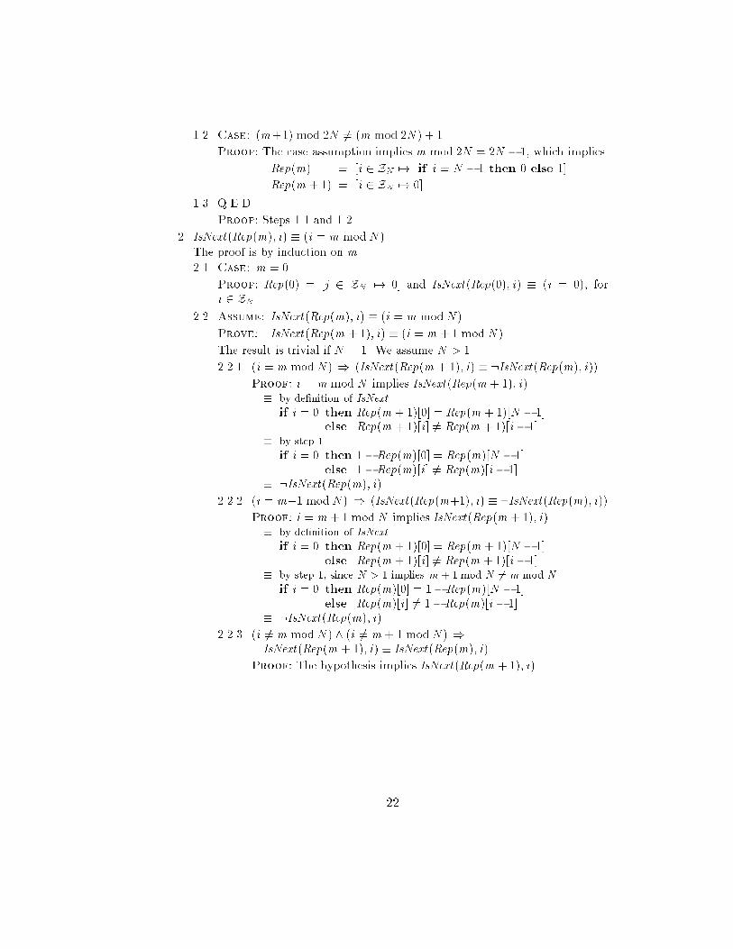
1.2. Case: (m+1) mod 2N 6= (m mod 2N ) + 1
Proof: The case assumption implies m mod 2N = 2N � 1, which implies
Rep(m) = [i 2 ZN 7! if i = N � 1 then 0 else 1]
Rep(m + 1) = [i 2 ZN 7! 0]
1.3. Q.E.D.
Proof: Steps 1.1 and 1.2.
2. IsNext(Rep(m); i) � (i = m mod N )
The proof is by induction on m.
2.1. Case: m = 0
Proof: Rep(0) = [j 2 ZN 7! 0] and IsNext(Rep(0); i) � (i = 0), for
i 2 ZN .
2.2. Assume: IsNext(Rep(m); i) � (i = m mod N )
Prove: IsNext(Rep(m + 1); i) � (i = m + 1 mod N )
The result is trivial if N = 1. We assume N > 1.
2.2.1. (i = m mod N ) ) (IsNext(Rep(m + 1); i) � :IsNext(Rep(m); i))
Proof: i = m mod N implies IsNext(Rep(m + 1); i)
� by de�nition of IsNext
if i = 0 then Rep(m + 1)[0] = Rep(m + 1)[N � 1]
else Rep(m + 1)[i ] 6= Rep(m + 1)[i � 1]
� by step 1
if i = 0 then 1�Rep(m)[0] = Rep(m)[N � 1]
else 1�Rep(m)[i ] 6= Rep(m)[i � 1]
� :IsNext(Rep(m); i)
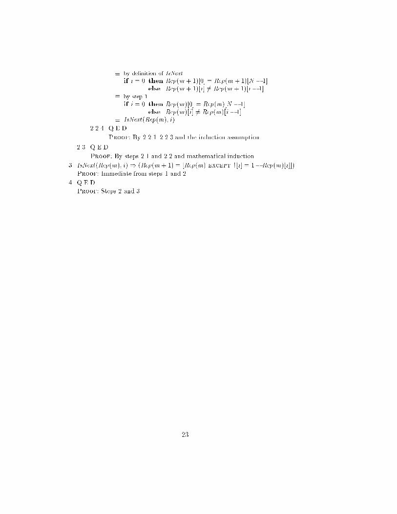
2.2.2. (i = m+1 mod N ) ) (IsNext(Rep(m+1); i) � :IsNext(Rep(m); i))
Proof: i = m + 1 mod N implies IsNext(Rep(m + 1); i)
� by de�nition of IsNext
if i = 0 then Rep(m + 1)[0] = Rep(m + 1)[N � 1]
else Rep(m + 1)[i ] 6= Rep(m + 1)[i � 1]
� by step 1, since N > 1 implies m + 1 mod N 6= m mod N
if i = 0 then Rep(m)[0] = 1�Rep(m)[N � 1]
else Rep(m)[i ] 6= 1�Rep(m)[i � 1]
� :IsNext(Rep(m); i)
2.2.3. (i 6= m mod N ) ^ (i 6= m + 1 mod N ) )
IsNext(Rep(m + 1); i) � IsNext(Rep(m); i)
Proof: The hypothesis implies IsNext(Rep(m + 1); i)
22
� by de�nition of IsNext
if i = 0 then Rep(m + 1)[0] = Rep(m + 1)[N � 1]
else Rep(m + 1)[i ] 6= Rep(m + 1)[i � 1]
� by step 1
if i = 0 then Rep(m)[0] = Rep(m)[N � 1]
else Rep(m)[i ] 6= Rep(m)[i � 1]
� IsNext(Rep(m); i)
2.2.4. Q.E.D.
Proof: By 2.2.1{2.2.3 and the induction assumption.
2.3 Q.E.D.
Proof: By steps 2.1 and 2.2 and mathematical induction.
3. IsNext(Rep(m); i)) (Rep(m + 1) = [Rep(m) except ![i ] = 1� Rep(m)[i ]])
Proof: Immediate from steps 1 and 2.
4. Q.E.D.
Proof: Steps 2 and 3.
23
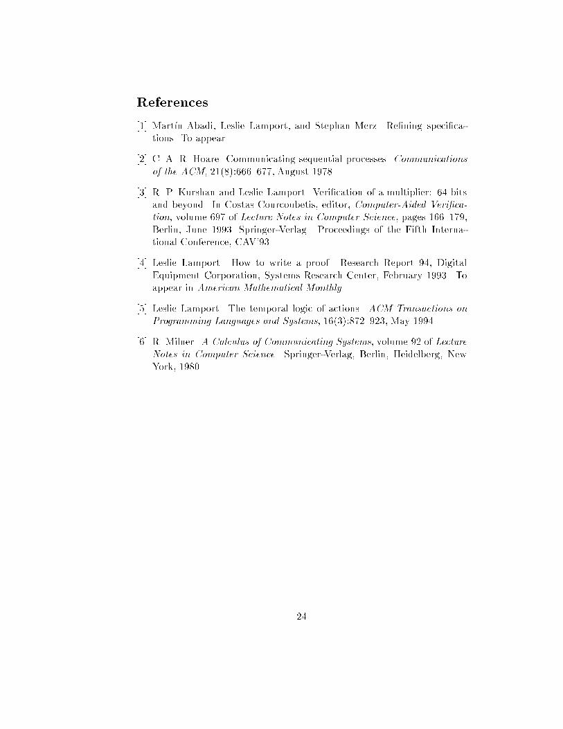
References
[1] Mart��n Abadi, Leslie Lamport, and Stephan Merz. Re�ning speci�ca-
tions. To appear.
[2] C. A. R. Hoare. Communicating sequential processes. Communications
of the ACM, 21(8):666{677, August 1978.
[3] R. P. Kurshan and Leslie Lamport. Veri�cation of a multiplier: 64 bits
and beyond. In Costas Courcoubetis, editor, Computer-Aided Veri�ca-
tion, volume 697 of Lecture Notes in Computer Science, pages 166{179,
Berlin, June 1993. Springer-Verlag. Proceedings of the Fifth Interna-
tional Conference, CAV'93.
[4] Leslie Lamport. How to write a proof. Research Report 94, Digital
Equipment Corporation, Systems Research Center, February 1993. To
appear in American Mathematical Monthly.
[5] Leslie Lamport. The temporal logic of actions. ACM Transactions on
Programming Languages and Systems, 16(3):872{923, May 1994.
[6] R. Milner. A Calculus of Communicating Systems, volume 92 of Lecture
Notes in Computer Science. Springer-Verlag, Berlin, Heidelberg, New
York, 1980.
24