Microeconomics

Andras Niedermayer

Université de Cergy-Pontoise

Fall 2019

1

Text Book

2

Pindyck, Robert S. and Daniel L.

Rubinfeld, Microeconomics,

Pearson International, 7th edition.

We will cover most of:

•Chapter 3: Consumer behaviour.

•Chapter 4: Individual & market demand.

•Sections 7.1-7.2: The cost of production.

•Chapter 8: Profit maximization & supply.

•Chapter 9: Welfare & surplus analysis of

competitive markets.

•Chapter 10: Monopoly and monopsony.

•Chapter 11: Market power and price

discrimination.

•Chapter 12: Monopolistic Competition

and Oligopoly

Additional Reading Material

Jean Tirole, Economics for the

Common Good, Princeton

University Press.

Please read these chapters:

•Chapter 13: Competition Policy and

Industrial Policy.

•Chapter 16: Innovation and Industrial

Policy.

•Chapter 17: Sector Regulation.

Grading system• Mid-term exam: 1/3 (November 4)

• Final exam: 2/3

4

Course organizationWe will have 12 classes of 2½ hours each.

Advice:

• Read the recommended sections of the text before class.

Come to class prepared to ask questions. Print out slides

from PDF file (available on webpage) before class.

• During class, take advantage of being in a small group to

ask questions. Take notes on the slide printout. Be an

active learner.

• After each class, review the exercises solved in class, and

solve the other assigned problems.

• Presentation slides and problem sets can be found at:o http://andras.niedermayer.ch/teaching

o Password: chenes

5

Change of Schedule• No classes on October 10 and October 17

• Replacement classes to be found

Consumer theory

Revision7

Chapter 3. Consumer Behaviour

● Theory of consumer behaviour: The description of how

each consumer allocates her income among different goods

and services to maximize her well-being.

Consumer behaviour is best understood in three distinct steps:

1. Consumer preferences (utility function, indifference curves)

2. Budget constraints

3. Consumer choices (constrained optimization)

8

The indifference curve U1 that

passes through market basket A

shows all baskets that give the

consumer the same level of

satisfaction as does market

basket A; these include baskets

B and D.

An Indifference Curve

Section 3.1: CONSUMER PREFERENCES

• Indifference Curves

● Indifference curve: A curve representing all combinations of

market baskets that provide a consumer with the same level of

satisfaction.

Our consumer prefers basket E,

which lies above U1, to A, but

prefers A to H or G, which lie

below U1.

9

An indifference map is a set of

indifference curves that

describes a person's

preferences.

An Indifference Map

CONSUMER PREFERENCES

• Indifference Maps

● indifference map: A graph containing a set of indifference curves

showing the market baskets among which a consumer is indifferent.

Any market basket on

indifference curve U3, such as

basket A, is preferred to any

basket on curve U2 (e.g., basket

B), which in turn is preferred to

any basket on U1, such as D.

10

If indifference curves U1 and U2

intersect, one of the

assumptions of consumer theory

is violated.

Indifference Curves Cannot Intersect

CONSUMER PREFERENCES

• Indifference Maps

According to this diagram, the

consumer should be indifferent

among market baskets A, B, and

D. Yet B should be preferred to

D because B has more of both

goods.

11

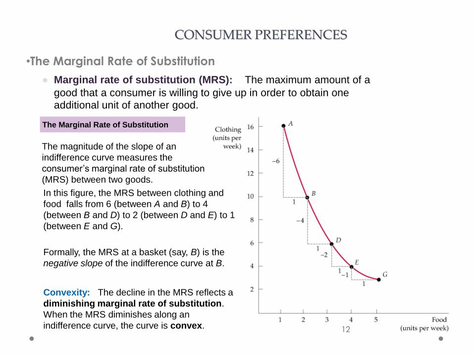
The magnitude of the slope of an

indifference curve measures the

consumer’s marginal rate of substitution

(MRS) between two goods.

The Marginal Rate of Substitution

CONSUMER PREFERENCES

•The Marginal Rate of Substitution

In this figure, the MRS between clothing and

food falls from 6 (between A and B) to 4

(between B and D) to 2 (between D and E) to 1

(between E and G).

Formally, the MRS at a basket (say, B) is the

negative slope of the indifference curve at B.

Convexity: The decline in the MRS reflects a

diminishing marginal rate of substitution.

When the MRS diminishes along an

indifference curve, the curve is convex.

● Marginal rate of substitution (MRS): The maximum amount of a

good that a consumer is willing to give up in order to obtain one

additional unit of another good.

12

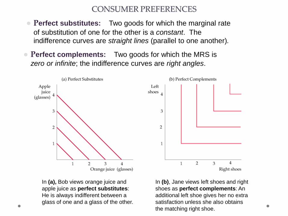
In (a), Bob views orange juice and

apple juice as perfect substitutes:

He is always indifferent between a

glass of one and a glass of the other.

CONSUMER PREFERENCES

In (b), Jane views left shoes and right

shoes as perfect complements: An

additional left shoe gives her no extra

satisfaction unless she also obtains

the matching right shoe.

● Perfect substitutes: Two goods for which the marginal rate

of substitution of one for the other is a constant. The indifference curves are straight lines (parallel to one another).

● Perfect complements: Two goods for which the MRS is

zero or infinite; the indifference curves are right angles.

CONSUMER PREFERENCES

● Bad: Good for which less is preferred rather than more.

(Examples: garbage, dirt, noise, pollution, disease, etc.)

• The negation of a “bad” is a “good” (e.g. sanitation, health)

Bads

14

CONSUMER PREFERENCES

• Utility and Utility Functions

A utility function can be represented by a

set of indifference curves, each with a

numerical indicator.

This figure shows three indifference curves

(with utility levels of 25, 50, and 100,

respectively) associated with the utility

function FC.

Important: Any labelling of the indifference

curves in strictly increasing order is a valid

utility function.

For example, instead of 25, 50, 100, we

could have assigned these three

indifference curves the utilities 5, 6, and 13.

● Utility: A numerical score representing the satisfaction that a

consumer gets from a given market basket.

● Utility function: A function that assigns a level of utility to each

individual market basket.

Utility Functions and Indifference Curves

15

Section 3.2: BUDGET CONSTRAINTS

• The Budget Line

A budget line describes the

combinations of goods that can be

purchased given the consumer’s

income and the prices of the goods.

Line AG (which passes through

points B, D, and E) shows the budget

associated with an income of $80, a

price of food of PF = $1 per unit, and

a price of clothing of PC = $2 per unit.

The slope of the budget line

(measured between points B and D)

is −PF / PC = −10/20 = −1/2.

If the prices PF and PC are fixed,

then clothing-consumption (C) can be

expressed as a linear function of

food-consumption (F) and income (I)

via the following linear equation:

A Budget Line

16

BUDGET CONSTRAINTS

• The Effects of Changes in Income and Prices

Income Changes A change in

income (with prices unchanged)

causes the budget line to shift

parallel to the original line (L1).

When the income of $80 (on L1) is

increased to $160, the budget line

shifts outward to L2.

If the income falls to $40, the line

shifts inward to L3.

Effects of a Change in Income on the

Budget Line

17

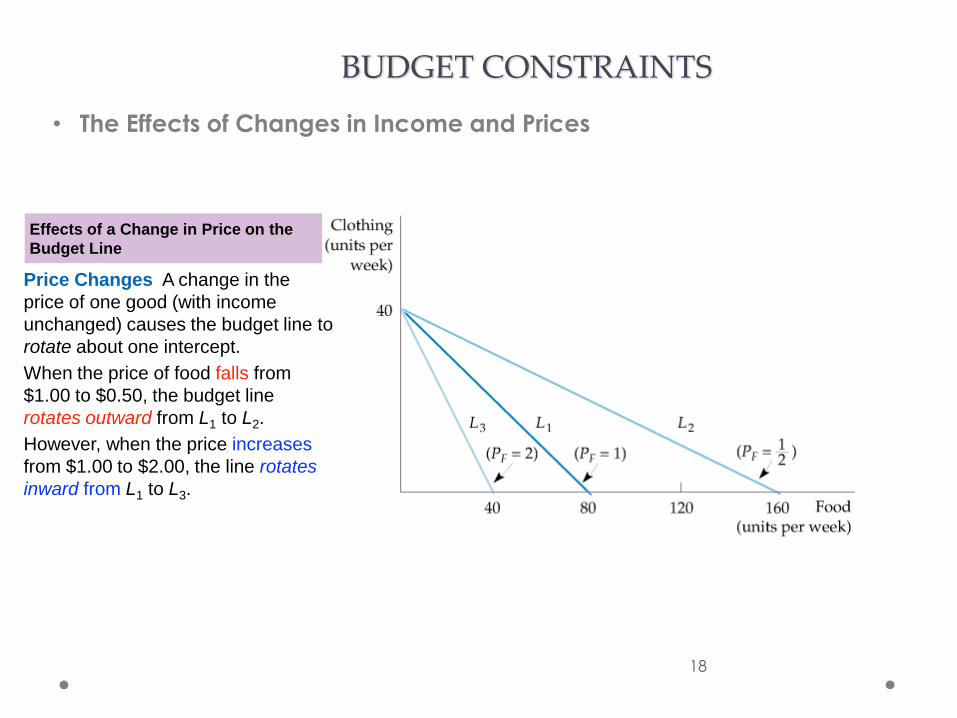
BUDGET CONSTRAINTS

• The Effects of Changes in Income and Prices

Price Changes A change in the

price of one good (with income

unchanged) causes the budget line to

rotate about one intercept.

When the price of food falls from

$1.00 to $0.50, the budget line

rotates outward from L1 to L2.

However, when the price increases

from $1.00 to $2.00, the line rotates

inward from L1 to L3.

Effects of a Change in Price on the

Budget Line

18

Section 3.3: CONSUMER CHOICE

A consumer maximizes satisfaction

by choosing market basket A. At this

point, the budget line and indifference

curve U2 are tangent.

Maximizing Consumer Satisfaction

The utility maximizing market basket must satisfy two conditions:

1. It must be located on the budget line.

2. It must give the consumer the most preferred combinationof goods and services.

No higher level of satisfaction (e.g.,

market basket D) can be attained.

At A, the point of maximization, the MRS

between the two goods equals the price

ratio.

At B, however, because the MRS

[− (−10/10) = 1] is greater than the price

ratio (1/2), satisfaction is not maximized.

19

Section 3.4: Marginal utility and consumer choice

● Also, note that MRS = MUF / MUC, where

MUF = marginal utility of food = Benefit from the

consumption of one additional unit of a good, and

MUC = marginal utility of clothing.

● Note that PF = marginal cost of food = cost of one

additional unit of a good.

Combining these equations, we get: MUF / MUC = PF / PC.

This is the kind of optimization condition that arises often in

economics. In this instance, satisfaction is maximized when the

ratio of marginal benefits equals the ratio of marginal costs.(Note: The book screws up the explanation by assuming PC = MUC = 1.)

Satisfaction is maximized (given the budget constraint) at the point where

● Meanwhile, PC = marginal cost of clothing.

20

CONSUMER CHOICE

• Corner Solutions

When the consumer’s marginal

rate of substitution is not equal to

the price ratio for all levels of

consumption, a corner solution

arises. The consumer maximizes

satisfaction by consuming only

one of the two goods.

Given budget line AB, the highest

level of satisfaction is achieved at

B on indifference curve U1, where

the MRS (of ice cream for frozen

yogurt) is greater than the ratio of

the price of ice cream to the price

of frozen yogurt.

Note: In a corner solution we do

not usually satisfy the equation

A Corner Solution

● Corner solution: A situation in which the marginal rate

of substitution of one good for another in a chosen market basket is not equal to the slope of the budget line.

21

Chapter 4:Individual and

Market Demand

22

Section 4.1: INDIVIDUAL DEMAND

Price Changes

Effect of Price Changes

A reduction in the price of food,

with income and the price of

clothing fixed, causes this

consumer to choose a different

market basket.

In (a), the baskets that maximize

utility for various prices of food

(point A, $2; B, $1; D, $0.50)

trace out the price-consumption

curve.

Part (b) gives the demand curve,

which relates the price of food to the

quantity demanded. (Points E, G, and H

correspond to points A, B, and D,

respectively).

23

Section 4.3: MARKET DEMAND

From Individual to Market Demand

Summing to Obtain a Market Demand

Curve

The market demand curve is

obtained by summing our three

consumers’ demand curves DA, DB,

and DC.

At each price, the quantity of coffee

demanded by the market is the

sum of the quantities demanded by

each consumer.

At a price of $4, for example, the

quantity demanded by the market

(11 units) is the sum of the quantity

demanded by A (no units), B (4

units), and C (7 units).

24

MARKET DEMAND

From Individual to Market Demand

The aggregation of individual demands into market demands

becomes important in practice when market demands are built up from

the demands of different demographic groups or from consumers

located in different areas.

For example, we might obtain information about the demand for home

computers by adding independently obtained information about the

demands of the following groups:

• Households with children

• Households without children

• Single individuals

Two points should be noted as a result of this analysis:

1. The market demand curve will shift to the right as more

consumers enter the market.

2. Factors that influence the demands of many consumers will also

affect market demand.

25

MARKET DEMAND

Elasticity of Demand

Denoting the quantity of a good by Q and its price by P, the price elasticity of demand is

Inelastic Demand

When demand is inelastic (i.e. Ep is less than one in absolute value),

the quantity demanded is relatively unresponsive to changes in price.

As a result, total expenditure on the product increases when the price increases. (Examples: necessities such as food, water, petrol.)

Elastic Demand

When demand is elastic (Ep is greater than one in absolute value),

total expenditure on the product decreases as the price goes up.(Examples: luxury items.)

% increase in demand= ——————————-

% increase in price

26

Welfare economics: Mainconcepts

• Consumer surplus (Section 4.4)

27

Section 4.4: Consumer surplus

Consider a consumer who purchases a quantity

Q of some good at some price P in the market.

The consumer surplus for this person is the

amount she benefits from being able to

purchase the quantity Q at the price P.

28

Consumer surplus: The case of indivisible goods (computation)

Maximum price the consumer

would be willing to pay:

◦ For the 1st unit: 100 euros

◦ For the 2nd unit: 85 euros

◦ For the 3rd unit: 50 euros

◦ For the 4th unit: 30 euros

If price = 20 euros, the consumer will buy 4 units.

“Total monetary value” for consuming 4 units :

100+85+50+30=265

Monetary cost for the 4 units bought :

20 x 4 =80

Surplus = 265-80=185 29

Demand

curve

Price

0 1 2 3 4 5

100

85

50

30

10

20

Caveat

• It is important to distinguish the price paid for a

good by a consumer and the monetary value of

this good for this consumer.

• Monetary value = maximum price the consumer

would be willing to pay for this good.

• Thus, the price paid is the lower bound for the

monetary value.

30

Consumer surplus: The case of divisible goods (pictorial)

31

C

B

A Quantity

Price

Demand

curve

P

O

Amount

paid by the

consumer

Surplus

• Assume quasi-linear utility U(x,y)=x+u(y) and income

R.

• A utility maximizer would spend all money, so that

the utility is u(y)+R-py

• The surplus is S= u(y)-u(0)-py.

Consumer surplus: computation (not in book)

Consumer surplus: computation (not in book)

o By definition, we have that:

o hence:

o Given that u’(y)=p(y), where u’(y) is the marginal utility and p(y) is the inverse demand function. (This comes from utility maximization.)

→surplus

= area of trianguloid region BCP

33

Aggregate consumers’ surplus

• Assume all consumers have quasilinear preferences.

• Consumers’ surplus = sum of the individual surpluses

• Graphically, area of trianguloid BCP (defined by the aggregate demand curve).

• Important Remark: we can “add” individual utilities because of our strong assumption on preferences (i.e. quasilinearity w.r.t. income) means that there is a common unit to measure utility for all the consumers (the Euro).

• This implies that utility transfers are possible though money transfers. (In real life, this is false).

34

Summary of Chapters 3 and 4• Consumers maximize utility subject to a budget constraint.

• At the optimal consumption bundle, the marginal rate of substitution

between two goods (the ratio of their marginal utilities) equals their price ratio. (i.e. the indifference curve is tangent to the budget line).

• Using this fact, we can derive each consumer’s demand as a function

of price (her demand curve) and her demand as a function of her

income (her Engel curve).

• The demand response to a price decrease is a sum of a substitution

effect (positive) and an income effect (possibly negative, if it is an

inferior good). Usually, the net effect is positive, so demand increases

as price decreases. (Exception: Giffen goods).

• The notion of consumer surplus depends on the hypothesis that the marginal utility of income is constant.

• Aggregate consumer surplus is the sum of individual surpluses.

• An allocation is Pareto efficient if there is ‘no waste’.

• Aggregate surplus is maximized in a Pareto efficient allocation.

We did not cover sections 3.4, 3.6, 4.5, and 4.6. 35

Chapter 3 Exercise 5• Suppose that Bridget and Erin spend their incomes on two

goods, food (F) and clothing (C). Bridget’s preferences are

represented by the utility function U(F,C) =10FC, while Erin’s

preferences are represented by the utility function

U(F,C)= .20 F2 C2.

• a. With food on the horizontal axis and clothing on the vertical

axis, identify on a graph the set of points that give Bridget the

same level of utility as the bundle (10, 5). Do the same for Erin

on a separate graph.

• b. On the same two graphs, identify the set of bundles that give Bridget and Erin the same level of utility as the bundle (15,

8).

• c. Do you think Bridget and Erin have the same preferences or

different preferences? Explain.

Chapter 3 Exercise 10• Antonio buys five new college textbooks during his

first year at school at a cost of $80 each. Used books

cost only $50 each. When the bookstore announces

that there will be a 10 percent increase in the price

of new books and a 5 percent increase in the price

of used books, Antonio’s father offers him $40 extra.

• a. What happens to Antonio’s budget line? Illustrate

the change with new books on the vertical axis.

• b. Is Antonio worse or better off after the price

change? Explain.

Chapter 3 Exercise 16• Julio receives utility from consuming food (F) and

clothing (C) as given by the utility function U(F,C)

FC. In addition, the price of food is $2 per unit, the

price of clothing is $10 per unit, and Julio’s weekly

income is $50.

• a. What is Julio’s marginal rate of substitution of food

for clothing when utility is maximized? Explain.

• b. Suppose instead that Julio is consuming a bundle

with more food and less clothing than his utility

maximizing bundle. Would his marginal rate of

substitution of food for clothing be greater than or

less than your answer in part a? Explain.