principles of quantum mechanics · 2006. 11. 25. · 2.3 expectation values of dynamical quantities...

PRINCIPLES OF

QUANTUM MECHANICS

as Applied to Chemistry and Chemical Physics

DONALD D. FITTS

University of Pennsylvania

pu bl i s h ed by th e pr e s s s y ndicat e of th e u n i v e r s i t y of cam br i dg eThe Pitt Building, Trumpington Street, Cambridge, United Kingdom

cambr i dg e u n i v e r s i t y pr e s sThe Edinburgh Building, Cambridge CB2 2RU, UK www.cup.cam.ac.uk

40 West 20th Street, New York, NY 10011-4211, USA www.cup.org10 Stamford Road, Oakleigh, Melbourne 3166, Australia

# D. D. Fitts 1999

This book is in copyright. Subject to statutory exceptionand to the provisions of relevant collective licensing agreements,

no reproduction of any part may take place withoutthe written permission of Cambridge University Press.

First published 1999

Printed in the United Kingdom at the University Press, Cambridge

Typeset in Times 11=14pt, in 3B2 [KT]

A catalogue record for this book is available from the British Library

Library of Congress Cataloguing in Publication dataFitts, Donald D., 1932±

Principles of quantum mechanics: as applied to chemistry andchemical physics / Donald D. Fitts.

p. cm.Includes bibliographical references and index

ISBN 0 521 65124 7 (hc.). ± ISBN 0 521 65841 1 (pbk.)1. Quantum chemistry. I. Title.

QD462.F55 1999541.298±dc21 98-39486 CIP

ISBN 0 521 65124 7 hardbackISBN 0 521 65841 1 paperback

Contents

Preface viii

Chapter 1 The wave function 1

1.1 Wave motion 2

1.2 Wave packet 8

1.3 Dispersion of a wave packet 15

1.4 Particles and waves 18

1.5 Heisenberg uncertainty principle 21

1.6 Young's double-slit experiment 23

1.7 Stern±Gerlach experiment 26

1.8 Physical interpretation of the wave function 29

Problems 34

Chapter 2 SchroÈdinger wave mechanics 36

2.1 The SchroÈdinger equation 36

2.2 The wave function 37

2.3 Expectation values of dynamical quantities 41

2.4 Time-independent SchroÈdinger equation 46

2.5 Particle in a one-dimensional box 48

2.6 Tunneling 53

2.7 Particles in three dimensions 57

2.8 Particle in a three-dimensional box 61

Problems 64

Chapter 3 General principles of quantum theory 65

3.1 Linear operators 65

3.2 Eigenfunctions and eigenvalues 67

3.3 Hermitian operators 69

v

3.4 Eigenfunction expansions 75

3.5 Simultaneous eigenfunctions 77

3.6 Hilbert space and Dirac notation 80

3.7 Postulates of quantum mechanics 85

3.8 Parity operator 94

3.9 Hellmann±Feynman theorem 96

3.10 Time dependence of the expectation value 97

3.11 Heisenberg uncertainty principle 99

Problems 104

Chapter 4 Harmonic oscillator 106

4.1 Classical treatment 106

4.2 Quantum treatment 109

4.3 Eigenfunctions 114

4.4 Matrix elements 121

4.5 Heisenberg uncertainty relation 125

4.6 Three-dimensional harmonic oscillator 125

Problems 128

Chapter 5 Angular momentum 130

5.1 Orbital angular momentum 130

5.2 Generalized angular momentum 132

5.3 Application to orbital angular momentum 138

5.4 The rigid rotor 148

5.5 Magnetic moment 151

Problems 155

Chapter 6 The hydrogen atom 156

6.1 Two-particle problem 157

6.2 The hydrogen-like atom 160

6.3 The radial equation 161

6.4 Atomic orbitals 175

6.5 Spectra 187

Problems 192

Chapter 7 Spin 194

7.1 Electron spin 194

7.2 Spin angular momentum 196

7.3 Spin one-half 198

7.4 Spin±orbit interaction 201

Problems 206

vi Contents

Chapter 8 Systems of identical particles 208

8.1 Permutations of identical particles 208

8.2 Bosons and fermions 217

8.3 Completeness relation 218

8.4 Non-interacting particles 220

8.5 The free-electron gas 226

8.6 Bose±Einstein condensation 229

Problems 230

Chapter 9 Approximation methods 232

9.1 Variation method 232

9.2 Linear variation functions 237

9.3 Non-degenerate perturbation theory 239

9.4 Perturbed harmonic oscillator 246

9.5 Degenerate perturbation theory 248

9.6 Ground state of the helium atom 256

Problems 260

Chapter 10 Molecular structure 263

10.1 Nuclear structure and motion 263

10.2 Nuclear motion in diatomic molecules 269

Problems 279

Appendix A Mathematical formulas 281

Appendix B Fourier series and Fourier integral 285

Appendix C Dirac delta function 292

Appendix D Hermite polynomials 296

Appendix E Legendre and associated Legendre polynomials 301

Appendix F Laguerre and associated Laguerre polynomials 310

Appendix G Series solutions of differential equations 318

Appendix H Recurrence relation for hydrogen-atom expectation values 329

Appendix I Matrices 331

Appendix J Evaluation of the two-electron interaction integral 341

Selected bibliography 344

Index 347

Physical constants

Contents vii

1

The wave function

Quantum mechanics is a theory to explain and predict the behavior of particles

such as electrons, protons, neutrons, atomic nuclei, atoms, and molecules, as

well as the photon±the particle associated with electromagnetic radiation or

light. From quantum theory we obtain the laws of chemistry as well as

explanations for the properties of materials, such as crystals, semiconductors,

superconductors, and super¯uids. Applications of quantum behavior give us

transistors, computer chips, lasers, and masers. The relatively new ®eld of

molecular biology, which leads to our better understanding of biological

structures and life processes, derives from quantum considerations. Thus,

quantum behavior encompasses a large fraction of modern science and tech-

nology.

Quantum theory was developed during the ®rst half of the twentieth century

through the efforts of many scientists. In 1926, E. SchroÈdinger interjected wave

mechanics into the array of ideas, equations, explanations, and theories that

were prevalent at the time to explain the growing accumulation of observations

of quantum phenomena. His theory introduced the wave function and the

differential wave equation that it obeys. SchroÈdinger's wave mechanics is now

the backbone of our current conceptional understanding and our mathematical

procedures for the study of quantum phenomena.

Our presentation of the basic principles of quantum mechanics is contained

in the ®rst three chapters. Chapter 1 begins with a treatment of plane waves

and wave packets, which serves as background material for the subsequent

discussion of the wave function for a free particle. Several experiments, which

lead to a physical interpretation of the wave function, are also described. In

Chapter 2, the SchroÈdinger differential wave equation is introduced and the

wave function concept is extended to include particles in an external potential

®eld. The formal mathematical postulates of quantum theory are presented in

Chapter 3.

1

1.1 Wave motion

Plane wave

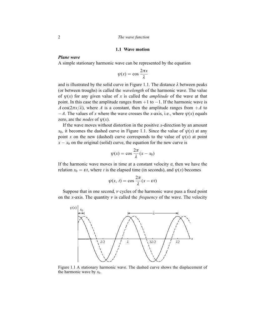
A simple stationary harmonic wave can be represented by the equation

ø(x) � cos2ðx

ë

and is illustrated by the solid curve in Figure 1.1. The distance ë between peaks

(or between troughs) is called the wavelength of the harmonic wave. The value

of ø(x) for any given value of x is called the amplitude of the wave at that

point. In this case the amplitude ranges from �1 to ÿ1. If the harmonic wave is

A cos(2ðx=ë), where A is a constant, then the amplitude ranges from �A to

ÿA. The values of x where the wave crosses the x-axis, i.e., where ø(x) equals

zero, are the nodes of ø(x).

If the wave moves without distortion in the positive x-direction by an amount

x0, it becomes the dashed curve in Figure 1.1. Since the value of ø(x) at any

point x on the new (dashed) curve corresponds to the value of ø(x) at point

xÿ x0 on the original (solid) curve, the equation for the new curve is

ø(x) � cos2ð

ë(xÿ x0)

If the harmonic wave moves in time at a constant velocity v, then we have the

relation x0 � vt, where t is the elapsed time (in seconds), and ø(x) becomes

ø(x, t) � cos2ð

ë(xÿ vt)

Suppose that in one second, í cycles of the harmonic wave pass a ®xed point

on the x-axis. The quantity í is called the frequency of the wave. The velocity

ψ(x) x0λ

λλ/2 3λ/2 λ2x

Figure 1.1 A stationary harmonic wave. The dashed curve shows the displacement ofthe harmonic wave by x0.

2 The wave function

v of the wave is then the product of í cycles per second and ë, the length of

each cycle

v � íë

and ø(x, t) may be written as

ø(x, t) � cos 2ðx

ëÿ ít

� �It is convenient to introduce the wave number k, de®ned as

k � 2ð

ë(1:1)

and the angular frequency ù, de®ned as

ù � 2ðí (1:2)

Thus, the velocity v becomes v � ù=k and the wave ø(x, t) takes the form

ø(x, t) � cos(kxÿ ùt)

The harmonic wave may also be described by the sine function

ø(x, t) � sin(kxÿ ùt)

The representation of ø(x, t) by the sine function is completely equivalent to

the cosine-function representation; the only difference is a shift by ë=4 in the

value of x when t � 0. Moreover, any linear combination of sine and cosine

representations is also an equivalent description of the simple harmonic wave.

The most general representation of the harmonic wave is the complex function

ø(x, t) � cos(kxÿ ùt)� i sin(kxÿ ùt) � ei(kxÿù t) (1:3)

where i equals��ÿ1p

and equation (A.31) from Appendix A has been intro-

duced. The real part, cos(kxÿ ùt), and the imaginary part, sin(kxÿ ùt), of the

complex wave, (1.3), may be readily obtained by the relations

Re [ei(kxÿù t)] � cos(kxÿ ùt) � 1

2[ø(x, t)� ø�(x, t)]

Im [ei(kxÿù t)] � sin(kxÿ ùt) � 1

2i[ø(x, t)ÿ ø�(x, t)]

where ø�(x, t) is the complex conjugate of ø(x, t)

ø�(x, t) � cos(kxÿ ùt)ÿ i sin(kxÿ ùt) � eÿi(kxÿù t)

The function ø�(x, t) also represents a harmonic wave moving in the positive

x-direction.

The functions exp[i(kx� ùt)] and exp[ÿi(kx� ùt)] represent harmonic

waves moving in the negative x-direction. The quantity (kx� ùt) is equal to

k(x� vt) or k(x� x0). After an elapsed time t, the value of the shifted

harmonic wave at any point x corresponds to the value at the point x� x0 at

time t � 0. Thus, the harmonic wave has moved in the negative x-direction.

1.1 Wave motion 3

The moving harmonic wave ø(x, t) in equation (1.3) is also known as a

plane wave. The quantity (kxÿ ùt) is called the phase. The velocity ù=k is

known as the phase velocity and henceforth is designated by vph, so that

vph � ù

k(1:4)

Composite wave

A composite wave is obtained by the addition or superposition of any number

of plane waves

Ø(x, t) �Xn

j�1

Ajei(k j xÿù j t) (1:5)

where Aj are constants. Equation (1.5) is a Fourier series representation of

Ø(x, t). Fourier series are discussed in Appendix B. The composite wave

Ø(x, t) is not a moving harmonic wave, but rather a superposition of n plane

waves with different wavelengths and frequencies and with different ampli-

tudes Aj. Each plane wave travels with its own phase velocity vph, j, such that

vph, j � ù j

kj

As a consequence, the pro®le of this composite wave changes with time. The

wave numbers kj may be positive or negative, but we will restrict the angular

frequencies ù j to positive values. A plane wave with a negative value of k has

a negative value for its phase velocity and corresponds to a harmonic wave

moving in the negative x-direction. In general, the angular frequency ùdepends on the wave number k. The dependence of ù(k) is known as the law

of dispersion for the composite wave.

In the special case where the ratio ù(k)=k is the same for each of the

component plane waves, so thatù1

k1

� ù2

k2

� � � � � ùn

k n

then each plane wave moves with the same velocity. Thus, the pro®le of the

composite wave does not change with time even though the angular frequencies

and the wave numbers differ. For this undispersed wave motion, the angular

frequency ù(k) is proportional to jkjù(k) � cjkj (1:6)

where c is a constant and, according to equation (1.4), is the phase velocity of

each plane wave in the composite wave. Examples of undispersed wave motion

are a beam of light of mixed frequencies traveling in a vacuum and the

undamped vibrations of a stretched string.

4 The wave function

For dispersive wave motion, the angular frequency ù(k) is not proportional

to |k|, so that the phase velocity vph varies from one component plane wave to

another. Since the phase velocity in this situation depends on k, the shape of

the composite wave changes with time. An example of dispersive wave motion

is a beam of light of mixed frequencies traveling in a dense medium such as

glass. Because the phase velocity of each monochromatic plane wave depends

on its wavelength, the beam of light is dispersed, or separated onto its

component waves, when passed through a glass prism. The wave on the surface

of water caused by dropping a stone into the water is another example of

dispersive wave motion.

Addition of two plane waves

As a speci®c and yet simple example of composite-wave construction and

behavior, we now consider in detail the properties of the composite wave

Ø(x, t) obtained by the addition or superposition of the two plane waves

exp[i(k1xÿ ù1 t)] and exp[i(k2xÿ ù2 t)]

Ø(x, t) � ei(k1 xÿù1 t) � ei(k2 xÿù2 t) (1:7)

We de®ne the average values k and ù and the differences Äk and Äù for the

two plane waves in equation (1.7) by the relations

k � k1 � k2

2ù � ù1 � ù2

2Äk � k1 ÿ k2 Äù � ù1 ÿ ù2

so that

k1 � k � Äk

2, k2 � k ÿ Äk

2

ù1 � ù� Äù

2, ù2 � ùÿ Äù

2

Using equation (A.32) from Appendix A, we may now write equation (1.7) in

the form

Ø(x, t) � ei(kxÿù t)[ei(ÄkxÿÄù t)=2 � eÿi(ÄkxÿÄù t)=2]

� 2 cosÄkxÿ Äùt

2

� �ei(kxÿù t) (1:8)

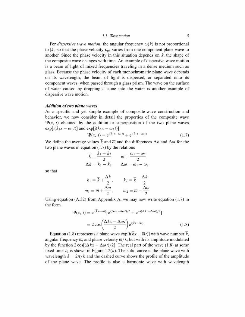
Equation (1.8) represents a plane wave exp[i(kxÿ ùt)] with wave number k,

angular frequency ù, and phase velocity ù=k, but with its amplitude modulated

by the function 2 cos[(Äkxÿ Äùt)=2]. The real part of the wave (1.8) at some

®xed time t0 is shown in Figure 1.2(a). The solid curve is the plane wave with

wavelength ë � 2ð=k and the dashed curve shows the pro®le of the amplitude

of the plane wave. The pro®le is also a harmonic wave with wavelength

1.1 Wave motion 5

4ð=Äk. At the points of maximum amplitude, the two original plane waves

interfere constructively. At the nodes in Figure 1.2(a), the two original plane

waves interfere destructively and cancel each other out.

As time increases, the plane wave exp[i(kxÿ ùt)] moves with velocity ù=k.

If we consider a ®xed point x1 and watch the plane wave as it passes that point,

we observe not only the periodic rise and fall of the amplitude of the

unmodi®ed plane wave exp[i(kxÿ ùt)], but also the overlapping rise and fall

of the amplitude due to the modulating function 2 cos[(Äkxÿ Äùt)=2]. With-

out the modulating function, the plane wave would reach the same maximum

2πk

4π/∆kRe Ψ(x, t)

(a)

x

Figure 1.2 (a) The real part of the superposition of two plane waves is shown by thesolid curve. The pro®le of the amplitude is shown by the dashed curve. (b) Thepositions of the curves in Figure 1.2(a) after a short time interval.

Re Ψ(x, t)

x

(b)

6 The wave function

and the same minimum amplitude with the passage of each cycle. The

modulating function causes the maximum (or minimum) amplitude for each

cycle of the plane wave to oscillate with frequency Äù=2.

The pattern in Figure 1.2(a) propagates along the x-axis as time progresses.

After a short period of time Ät, the wave (1.8) moves to a position shown in

Figure 1.2(b). Thus, the position of maximum amplitude has moved in the

positive x-direction by an amount vgÄt, where vg is the group velocity of the

composite wave, and is given by

vg � Äù

Äk(1:9)

The expression (1.9) for the group velocity of a composite of two plane waves

is exact.

In the special case when k2 equals ÿk1 and ù2 equals ù1 in equation (1.7),

the superposition of the two plane waves becomes

Ø(x, t) � ei(kxÿù t) � eÿi(kx�ù t) (1:10)

where

k � k1 � ÿk2

ù � ù1 � ù2

The two component plane waves in equation (1.10) travel with equal phase

velocities ù=k, but in opposite directions. Using equations (A.31) and (A.32),

we can express equation (1.10) in the form

Ø(x, t) � (eikx � eÿikx)eÿiù t

� 2 cos kx eÿiù t

� 2 cos kx (cosùt ÿ i sinùt)

We see that for this special case the composite wave is the product of two

functions: one only of the distance x and the other only of the time t. The

composite wave Ø(x, t) vanishes whenever cos kx is zero, i.e., when kx � ð=2,

3ð=2, 5ð=2, . . . , regardless of the value of t. Therefore, the nodes of Ø(x, t)

are independent of time. However, the amplitude or pro®le of the composite

wave changes with time. The real part of Ø(x, t) is shown in Figure 1.3. The

solid curve represents the wave when cosùt is a maximum, the dotted curve

when cosùt is a minimum, and the dashed curve when cosùt has an

intermediate value. Thus, the wave does not travel, but pulsates, increasing and

decreasing in amplitude with frequency ù. The imaginary part of Ø(x, t)

behaves in the same way. A composite wave with this behavior is known as a

standing wave.

1.1 Wave motion 7

1.2 Wave packet

We now consider the formation of a composite wave as the superposition of a

continuous spectrum of plane waves with wave numbers k con®ned to a narrow

band of values. Such a composite wave Ø(x, t) is known as a wave packet and

may be expressed as

Ø(x, t) � 1��2ðp

�1ÿ1

A(k)ei(kxÿù t)dk (1:11)

The weighting factor A(k) for each plane wave of wave number k is negligible

except when k lies within a small interval Äk. For mathematical convenience

we have included a factor (2ð)ÿ1=2 on the right-hand side of equation (1.11).

This factor merely changes the value of A(k) and has no other effect.

We note that the wave packet Ø(x, t) is the inverse Fourier transform of

A(k). The mathematical development and properties of Fourier transforms are

presented in Appendix B. Equation (1.11) has the form of equation (B.19).

According to equation (B.20), the Fourier transform A(k) is related to Ø(x, t)

by

A(k) � 1��2ðp

�1ÿ1

Ø(x, t)eÿi(kxÿù t) dx (1:12)

It is because of the Fourier relationships between Ø(x, t) and A(k) that the

factor (2ð)ÿ1=2 is included in equation (1.11). Although the time t appears in

the integral on the right-hand side of (1.12), the function A(k) does not depend

on t; the time dependence of Ø(x, t) cancels the factor eiù t. We consider below

Re Ψ(x, t)

x

Figure 1.3 A standing harmonic wave at various times.

8 The wave function

two speci®c examples for the functional form of A(k). However, in order to

evaluate the integral over k in equation (1.11), we also need to know the

dependence of the angular frequency ù on the wave number k.

In general, the angular frequency ù(k) is a function of k, so that the angular

frequencies in the composite wave Ø(x, t), as well as the wave numbers, vary

from one plane wave to another. If ù(k) is a slowly varying function of k and

the values of k are con®ned to a small range Äk, then ù(k) may be expanded

in a Taylor series in k about some point k0 within the interval Äk

ù(k) � ù0 � dù

dk

� �0

(k ÿ k0)� 1

2

d2ù

dk2

� �0(k ÿ k0)2 � � � � (1:13)

where ù0 is the value of ù(k) at k0 and the derivatives are also evaluated at k0.

We may neglect the quadratic and higher-order terms in the Taylor expansion

(1.13) because the interval Äk and, consequently, k ÿ k0 are small. Substitu-

tion of equation (1.13) into the phase for each plane wave in (1.11) then gives

kxÿ ùt � (k ÿ k0 � k0)xÿ ù0 t ÿ dù

dk

� �0

(k ÿ k0)t

� k0xÿ ù0 t � xÿ dù

dk

� �0

t

" #(k ÿ k0)

so that equation (1.11) becomes

Ø(x, t) � B(x, t)ei(k0 xÿù0 t) (1:14)

where

B(x, t) � 1��2ðp

�1ÿ1

A(k)ei[xÿ(dù=dk)0 t](kÿk0) dk (1:15)

Thus, the wave packet Ø(x, t) represents a plane wave of wave number k0 and

angular frequency ù0 with its amplitude modulated by the factor B(x, t). This

modulating function B(x, t) depends on x and t through the relationship

[xÿ (dù=dk)0 t]. This situation is analogous to the case of two plane waves as

expressed in equations (1.7) and (1.8). The modulating function B(x, t) moves

in the positive x-direction with group velocity vg given by

vg � dù

dk

� �0

(1:16)

In contrast to the group velocity for the two-wave case, as expressed in

equation (1.9), the group velocity in (1.16) for the wave packet is not uniquely

de®ned. The point k0 is chosen arbitrarily and, therefore, the value at k0 of the

derivative dù=dk varies according to that choice. However, the range of k is

1.2 Wave packet 9

narrow and ù(k) changes slowly with k, so that the variation in vg is small.

Combining equations (1.15) and (1.16), we have

B(x, t) � 1��2ðp

�1ÿ1

A(k)ei(xÿvg t)(kÿk0) dk (1:17)

Since the function A(k) is the Fourier transform of Ø(x, t), the two functions

obey Parseval's theorem as given by equation (B.28) in Appendix B�1ÿ1jØ(x, t)j2dx �

�1ÿ1jB(x, t)j2 dx �

�1ÿ1jA(k)j2 dk (1:18)

Gaussian wave number distribution

In order to obtain a speci®c mathematical expression for the wave packet, we

need to select some form for the function A(k). In our ®rst example we choose

A(k) to be the gaussian function

A(k) � 1��2ðp

áeÿ(kÿk0)2=2á2

(1:19)

This function A(k) is a maximum at wave number k0, which is also the average

value for k for this distribution of wave numbers. Substitution of equation

(1.19) into (1.17) gives

jØ(x, t)j � B(x, t) � 1��2ðp eÿá

2(xÿvg t)2=2 (1:20)

where equation (A.8) has been used. The resulting modulating factor B(x, t) is

also a gaussian function±following the general result that the Fourier transform

of a gaussian function is itself gaussian. We have also noted in equation (1.20)

that B(x, t) is always positive and is therefore equal to the absolute value

jØ(x, t)j of the wave packet. The functions A(k) and jØ(x, t)j are shown in

Figure 1.4.

Figure 1.4 (a) A gaussian wave number distribution. (b) The modulating functioncorresponding to the wave number distribution in Figure 1.4(a).

A(k)1/√2π α

1/√2π αe

kk0k0 2 √2 α k0 1 √2 α(a)

1/√2π

1/√2π e

x

vg t 2(b)

|Ψ(x, t)|

√2α

vg t vg t 1 √2α

10 The wave function

Figure 1.5 shows the real part of the plane wave exp[i(k0xÿ ù0 t)] with its

amplitude modulated by B(x, t) of equation (1.20). The plane wave moves in

the positive x-direction with phase velocity vph equal to ù0=k0. The maximum

amplitude occurs at x � vg t and propagates in the positive x-direction with

group velocity vg equal to (dù=dk)0.

The value of the function A(k) falls from its maximum value of (��2ðp

á)ÿ1 at

k0 to 1=e of its maximum value when jk ÿ k0j equals��2p

á. Most of the area

under the curve (actually 84.3%) comes from the range

ÿ��2p

á, (k ÿ k0) ,��2p

á

Thus, the distance��2p

á may be regarded as a measure of the width of the

distribution A(k) and is called the half width. The half width may be de®ned

using 1=2 or some other fraction instead of 1=e. The reason for using 1=e is

that the value of k at that point is easily obtained without consulting a table of

numerical values. These various possible de®nitions give different numerical

values for the half width, but all these values are of the same order of

magnitude. Since the value of jØ(x, t)j falls from its maximum value of

(2ð)ÿ1=2 to 1=e of that value when jxÿ vg tj equals��2p

=á, the distance��2p

=ámay be considered the half width of the wave packet.

When the parameter á is small, the maximum of the function A(k) is high

and the function drops off in value rapidly on each side of k0, giving a small

value for the half width. The half width of the wave packet, however, is large

because it is proportional to 1=á. On the other hand, when the parameter á is

large, the maximum of A(k) is low and the function drops off slowly, giving a

large half width. In this case, the half width of the wave packet becomes small.

If we regard the uncertainty Äk in the value of k as the half width of the

distribution A(k) and the uncertainty Äx in the position of the wave packet as

its half width, then the product of these two uncertainties is

ÄxÄk � 2

x

Figure 1.5 The real part of a wave packet for a gaussian wave number distribution.

1.2 Wave packet 11

Thus, the product of these two uncertainties Äx and Äk is a constant of order

unity, independent of the parameter á.

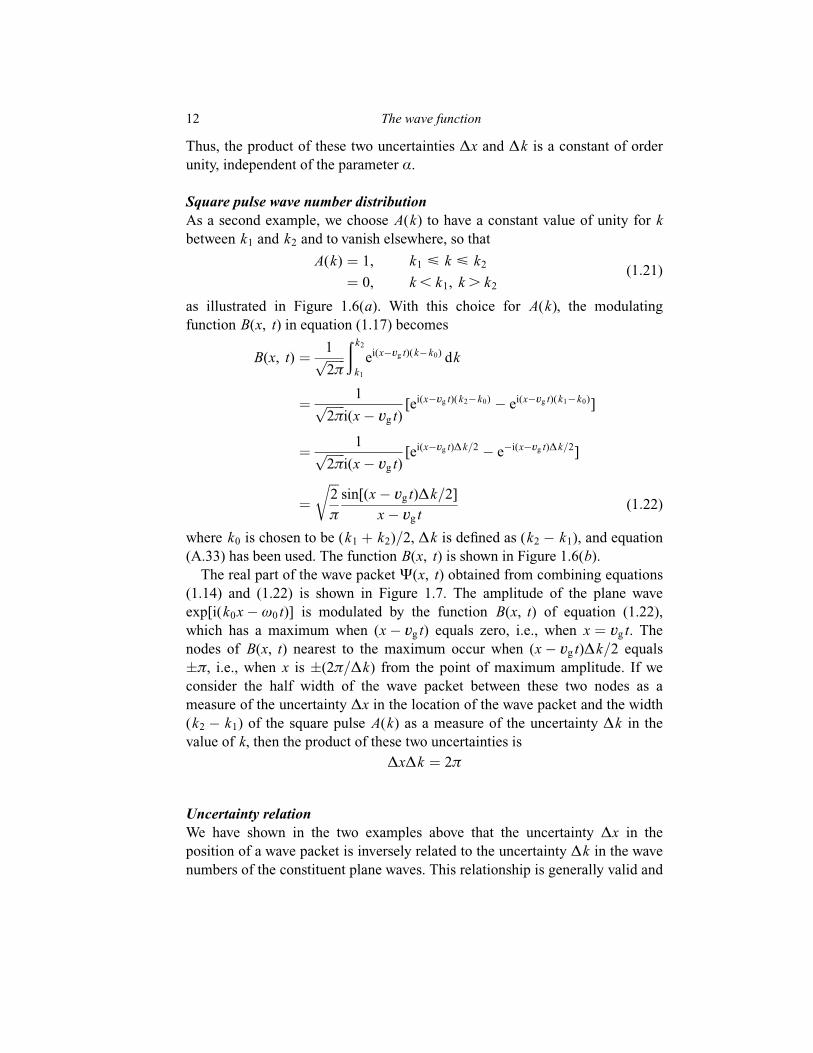
Square pulse wave number distribution

As a second example, we choose A(k) to have a constant value of unity for k

between k1 and k2 and to vanish elsewhere, so that

A(k) � 1, k1 < k < k2

� 0, k , k1, k . k2

(1:21)

as illustrated in Figure 1.6(a). With this choice for A(k), the modulating

function B(x, t) in equation (1.17) becomes

B(x, t) � 1��2ðp

� k2

k1

ei(xÿvg t)(kÿk0) dk

� 1��2ðp

i(xÿ vg t)[ei(xÿvg t)(k2ÿk0) ÿ ei(xÿvg t)(k1ÿk0)]

� 1��2ðp

i(xÿ vg t)[ei(xÿvg t)Äk=2 ÿ eÿi(xÿvg t)Äk=2]

��2

ð

rsin[(xÿ vg t)Äk=2]

xÿ vg t(1:22)

where k0 is chosen to be (k1 � k2)=2, Äk is de®ned as (k2 ÿ k1), and equation

(A.33) has been used. The function B(x, t) is shown in Figure 1.6(b).

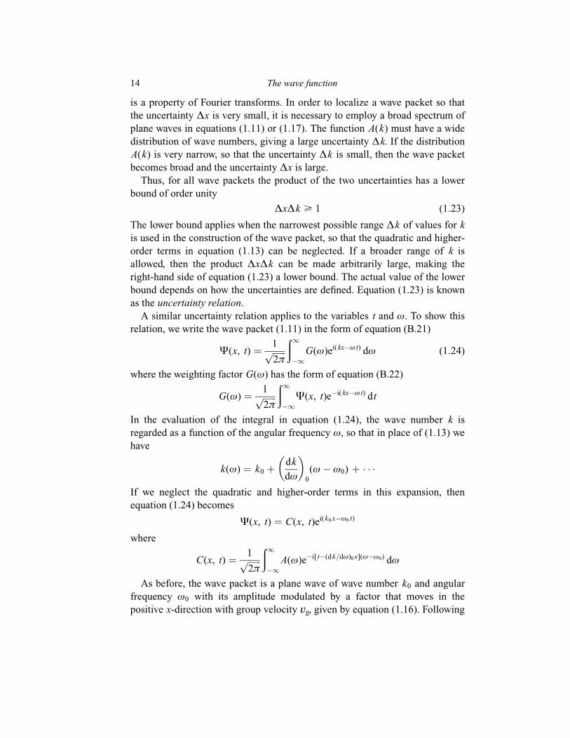
The real part of the wave packet Ø(x, t) obtained from combining equations

(1.14) and (1.22) is shown in Figure 1.7. The amplitude of the plane wave

exp[i(k0xÿ ù0 t)] is modulated by the function B(x, t) of equation (1.22),

which has a maximum when (xÿ vg t) equals zero, i.e., when x � vg t. The

nodes of B(x, t) nearest to the maximum occur when (xÿ vg t)Äk=2 equals

�ð, i.e., when x is �(2ð=Äk) from the point of maximum amplitude. If we

consider the half width of the wave packet between these two nodes as a

measure of the uncertainty Äx in the location of the wave packet and the width

(k2 ÿ k1) of the square pulse A(k) as a measure of the uncertainty Äk in the

value of k, then the product of these two uncertainties is

ÄxÄk � 2ð

Uncertainty relation

We have shown in the two examples above that the uncertainty Äx in the

position of a wave packet is inversely related to the uncertainty Äk in the wave

numbers of the constituent plane waves. This relationship is generally valid and


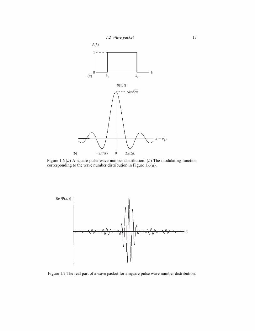
Figure 1.6 (a) A square pulse wave number distribution. (b) The modulating functioncorresponding to the wave number distribution in Figure 1.6(a).

A(k)

1

0k1 k2

k(a)

B(x, t)

∆k/√2π

x 2 vg t

022π/∆k 2π/∆k(b)

Re Ψ(x, t)

x

Figure 1.7 The real part of a wave packet for a square pulse wave number distribution.

1.2 Wave packet 13

is a property of Fourier transforms. In order to localize a wave packet so that

the uncertainty Äx is very small, it is necessary to employ a broad spectrum of

plane waves in equations (1.11) or (1.17). The function A(k) must have a wide

distribution of wave numbers, giving a large uncertainty Äk. If the distribution

A(k) is very narrow, so that the uncertainty Äk is small, then the wave packet

becomes broad and the uncertainty Äx is large.

Thus, for all wave packets the product of the two uncertainties has a lower

bound of order unity

ÄxÄk > 1 (1:23)

The lower bound applies when the narrowest possible range Äk of values for k

is used in the construction of the wave packet, so that the quadratic and higher-

order terms in equation (1.13) can be neglected. If a broader range of k is

allowed, then the product ÄxÄk can be made arbitrarily large, making the

right-hand side of equation (1.23) a lower bound. The actual value of the lower

bound depends on how the uncertainties are de®ned. Equation (1.23) is known

as the uncertainty relation.

A similar uncertainty relation applies to the variables t and ù. To show this

relation, we write the wave packet (1.11) in the form of equation (B.21)

Ø(x, t) � 1��2ðp

�1ÿ1

G(ù)ei(kxÿù t) dù (1:24)

where the weighting factor G(ù) has the form of equation (B.22)

G(ù) � 1��2ðp

�1ÿ1

Ø(x, t)eÿi(kxÿù t) dt

In the evaluation of the integral in equation (1.24), the wave number k is

regarded as a function of the angular frequency ù, so that in place of (1.13) we

have

k(ù) � k0 � dk

dù

� �0

(ùÿ ù0) � � � �

If we neglect the quadratic and higher-order terms in this expansion, then

equation (1.24) becomes

Ø(x, t) � C(x, t)ei(k0 xÿù0 t)

where

C(x, t) � 1��2ðp

�1ÿ1

A(ù)eÿi[ tÿ(dk=dù)0 x](ùÿù0) dù

As before, the wave packet is a plane wave of wave number k0 and angular

frequency ù0 with its amplitude modulated by a factor that moves in the

positive x-direction with group velocity vg, given by equation (1.16). Following


the previous analysis, if we select a speci®c form for the modulating function

G(ù) such as a gaussian or a square pulse distribution, we can show that the

product of the uncertainty Ät in the time variable and the uncertainty Äù in

the angular frequency of the wave packet has a lower bound of order unity, i.e.

ÄtÄù > 1 (1:25)

This uncertainty relation is also a property of Fourier transforms and is valid

for all wave packets.

1.3 Dispersion of a wave packet

In this section we investigate the change in contour of a wave packet as it

propagates with time.

The general expression for a wave packet Ø(x, t) is given by equation

(1.11). The weighting factor A(k) in (1.11) is the inverse Fourier transform of

Ø(x, t) and is given by (1.12). Since the function A(k) is independent of time,

we may set t equal to any arbitrary value in the integral on the right-hand side

of equation (1.12). If we let t equal zero in (1.12), then that equation becomes

A(k) � 1��2ðp

�1ÿ1

Ø(î, 0)eÿikî dî (1:26)

where we have also replaced the dummy variable of integration by î. Substitu-

tion of equation (1.26) into (1.11) yields

Ø(x, t) � 1

2ð

��1ÿ1

Ø(î, 0)ei[k(xÿî)ÿù t] dk dî (1:27)

Since the limits of integration do not depend on the variables î and k, the order

of integration over these variables may be interchanged.

Equation (1.27) relates the wave packet Ø(x, t) at time t to the wave packet

Ø(x, 0) at time t � 0. However, the angular frequency ù(k) is dependent on k

and the functional form must be known before we can evaluate the integral

over k.

If ù(k) is proportional to jkj as expressed in equation (1.6), then (1.27) gives

Ø(x, t) � 1

2ð

��1ÿ1

Ø(î, 0)eik(xÿctÿî) dk dî

The integral over k may be expressed in terms of the Dirac delta function

through equation (C.6) in Appendix C, so that we have


Ø(x, t) ��1ÿ1

Ø(î, 0)ä(xÿ ct ÿ î) dî � Ø(xÿ ct, 0)

Thus, the wave packet Ø(x, t) has the same value at point x and time t that it

had at point xÿ ct at time t � 0. The wave packet has traveled with velocity c

without a change in its contour, i.e., it has traveled without dispersion. Since

the phase velocity vph is given by ù0=k0 � c and the group velocity vg is given

by (dù=dk)0 � c, the two velocities are the same for an undispersed wave

packet.

We next consider the more general situation where the angular frequency

ù(k) is not proportional to jkj, but is instead expanded in the Taylor series

(1.13) about (k ÿ k0). Now, however, we retain the quadratic term, but still

neglect the terms higher than quadratic, so that

ù(k) � ù0 � vg(k ÿ k0)� ã(k ÿ k0)2

where equation (1.16) has been substituted for the ®rst-order derivative and ãis an abbreviation for the second-order derivative

ã � 1

2

d2ù

dk2

� �0

The phase in equation (1.27) then becomes

k(xÿ î)ÿ ùt � (k ÿ k0)(xÿ î)� k0(xÿ î)ÿ ù0 t

ÿ vg t(k ÿ k0)ÿ ãt(k ÿ k0)2

� k0xÿ ù0 t ÿ k0î� (xÿ vg t ÿ î)(k ÿ k0)ÿ ãt(k ÿ k0)2

so that the wave packet (1.27) takes the form

Øã(x, t) � ei(k0 xÿù0 t)

2ð

��1ÿ1

Ø(î, 0)eÿik0îei(xÿvg tÿî)(kÿk0)ÿiã t(kÿk0)2

dk dî

The subscript ã has been included in the notation Øã(x, t) in order to

distinguish that wave packet from the one in equations (1.14) and (1.15), where

the quadratic term in ù(k) is omitted. The integral over k may be evaluated

using equation (A.8), giving the result


2��iðãtp

��1ÿ1

Ø(î, 0)eÿik0îeÿ(xÿvg tÿî)2=4iã t dî (1:28)

Equation (1.28) relates the wave packet at time t to the wave packet at time

t � 0 if the k-dependence of the angular frequency includes terms up to k2.

The pro®le of the wave packet Øã(x, t) changes as time progresses because of


the factor tÿ1=2 before the integral and the t in the exponent within the integral.

If we select a speci®c form for the wave packet at time t � 0, the nature of this

time dependence becomes more evident.

Gaussian wave packet

Let us suppose that Ø(x, 0) has the gaussian distribution (1.20) as its pro®le, so

that equation (1.14) at time t � 0 is

Ø(î, 0) � eik0îB(î, 0) � 1��2ðp eik0îeÿá

2î2=2 (1:29)

Substitution of equation (1.29) into (1.28) gives


2ð��2iãtp

�1ÿ1

eÿá2î2=2eÿ(xÿvg tÿî)2=4iã t dî

The integral may be evaluated using equation (A.8) accompanied with some

tedious, but straightforward algebraic manipulations, yielding

Øã(x, t) � ei(k0 xÿù0 t)��2ð(1� 2iá2ãt)

p eÿá2(xÿvg t)2=2(1�2iá2ã t) (1:30)

The wave packet, then, consists of the plane wave exp i[k0xÿ ù0 t] with its

amplitude modulated by

1��2ð(1� 2iá2ãt)

p eÿá2(xÿvg t)2=2(1�2iá2ã t)

which is a complex function that depends on the time t. When ã equals zero so

that the quadratic term in ù(k) is neglected, this complex modulating function

reduces to B(x, t) in equation (1.20). The absolute value jØã(x, t)j of the wave

packet (1.30) is given by

jØã(x, t)j � 1

(2ð)1=2(1� 4á4ã2 t2)1=4eÿá

2(xÿvg t)2=2(1�4á4ã2 t2) (1:31)

We now contrast the behavior of the wave packet in equation (1.31) with that

of the wave packet in (1.20). At any time t, the maximum amplitudes of both

occur at x � vg t and travel in the positive x-direction with the same group

velocity vg. However, at that time t, the value of jØã(x, t)j is 1=e of its

maximum value when the exponent in equation (1.31) is unity, so that the half

width or uncertainty Äx for jØã(x, t)j is given by

Äx � jxÿ vg tj ��2p

á

��1� 4á4ã2 t2

pMoreover, the maximum amplitude for jØã(x, t)j at time t is given by

(2ð)ÿ1=2(1� 4á4ã2 t2)ÿ1=4


As time increases from ÿ1 to 0, the half width of the wave packet jØã(x, t)jcontinuously decreases and the maximum amplitude continuously increases. At

t � 0 the half width attains its lowest value of��2p

=á and the maximum

amplitude attains its highest value of 1=��2ðp

, and both values are in agreement

with the wave packet in equation (1.20). As time increases from 0 to 1, the

half width continuously increases and the maximum amplitude continuously

decreases. Thus, as t2 increases, the wave packet jØã(x, t)j remains gaussian

in shape, but broadens and ¯attens out in such a way that the area under the

square jØã(x, t)j2 of the wave packet remains constant over time at a value of

(2��ðp

á)ÿ1, in agreement with Parseval's theorem (1.18).

The product ÄxÄk for this spreading wave packet Øã(x, t) is

ÄxÄk � 2��1� 4á4ã2 t2

pand increases as jtj increases. Thus, the value of the right-hand side when t � 0

is the lower bound for the product ÄxÄk and is in agreement with the

uncertainty relation (1.23).

1.4 Particles and waves

To explain the photoelectric effect, Einstein (1905) postulated that light, or

electromagnetic radiation, consists of a beam of particles, each of which travels

at the same velocity c (the speed of light), where c has the value

c � 2:997 92 3 108 m sÿ1

Each particle, later named a photon, has a characteristic frequency í and an

energy hí, where h is Planck's constant with the value

h � 6:626 08 3 10ÿ34 J s

The constant h and the hypothesis that energy is quantized in integral multiples

of hí had previously been introduced by M. Planck (1900) in his study of

blackbody radiation.1 In terms of the angular frequency ù de®ned in equation

(1.2), the energy E of a photon is

E � "ù (1:32)

where " is de®ned by

" � h

2ð� 1:054 57 3 10ÿ34 J s

Because the photon travels with velocity c, its motion is governed by relativity

1 The history of the development of quantum concepts to explain observed physical phenomena, whichoccurred mainly in the ®rst three decades of the twentieth century, is discussed in introductory texts onphysical chemistry and on atomic physics. A much more detailed account is given in M. Jammer (1966)The Conceptual Development of Quantum Mechanics (McGraw-Hill, New York).


theory, which requires that its rest mass be zero. The magnitude of the

momentum p for a particle with zero rest mass is related to the relativistic

energy E by p � E=c, so that

p � E

c� hí

c� "ù

c

Since the velocity c equals ù=k, the momentum is related to the wave number

k for a photon by

p � "k (1:33)

Einstein's postulate was later con®rmed experimentally by A. Compton (1924).

Noting that it had been fruitful to regard light as having a corpuscular nature,

L. de Broglie (1924) suggested that it might be useful to associate wave-like

behavior with the motion of a particle. He postulated that a particle with linear

momentum p be associated with a wave whose wavelength ë is given by

ë � 2ð

k� h

p(1:34)

and that expressions (1.32) and (1.33) also apply to particles. The hypothesis of

wave properties for particles and the de Broglie relation (equation (1.34)) have

been con®rmed experimentally for electrons by G. P. Thomson (1927) and by

Davisson and Germer (1927), for neutrons by E. Fermi and L. Marshall (1947),

and by W. H. Zinn (1947), and for helium atoms and hydrogen molecules by I.

Estermann, R. Frisch, and O. Stern (1931).

The classical, non-relativistic energy E for a free particle, i.e., a particle in

the absence of an external force, is expressed as the sum of the kinetic and

potential energies and is given by

E � 1

2mv2 � V � p2

2m� V (1:35)

where m is the mass and v the velocity of the particle, the linear momentum p

is

p � mv

and V is a constant potential energy. The force F acting on the particle is given

by

F � ÿ dV

dx� 0

and vanishes because V is constant. In classical mechanics the choice of the

zero-level of the potential energy is arbitrary. Since the potential energy for the

free particle is a constant, we may, without loss of generality, take that constant

value to be zero, so that equation (1.35) becomes

1.4 Particles and waves 19

E � p2

2m(1:36)

Following the theoretical scheme of SchroÈdinger, we associate a wave packet

Ø(x, t) with the motion in the x-direction of this free particle. This wave

packet is readily constructed from equation (1.11) by substituting (1.32) and

(1.33) for ù and k, respectively

Ø(x, t) � 1��2ð"p

�1ÿ1

A( p)ei( pxÿEt)=" d p (1:37)

where, for the sake of symmetry between Ø(x, t) and A( p), a factor "ÿ1=2 has

been absorbed into A( p). The function A(k) in equation (1.12) is now

"1=2 A( p), so that

A( p) � 1��2ð"p

�1ÿ1

Ø(x, t)eÿi( pxÿEt)=" dx (1:38)

The law of dispersion for this wave packet may be obtained by combining

equations (1.32), (1.33), and (1.36) to give

ù(k) � E

"� p2

2m"� "k2

2m(1:39)

This dispersion law with ù proportional to k2 is different from that for

undispersed light waves, where ù is proportional to k.

If ù(k) in equation (1.39) is expressed as a power series in k ÿ k0, we obtain

ù(k) � "k20

2m� "k0

m(k ÿ k0)� "

2m(k ÿ k0)2 (1:40)

This expansion is exact; there are no terms of higher order than quadratic.

From equation (1.40) we see that the phase velocity vph of the wave packet is

given by

vph � ù0

k0

� "k0

2m(1:41)

and the group velocity vg is

vg � dù

dk

� �0

� "k0

m(1:42)

while the parameter ã of equations (1.28), (1.30), and (1.31) is

ã � 1

2

d2ù

dk2

� �0� "

2m(1:43)

If we take the derivative of ù(k) in equation (1.39) with respect to k and use

equation (1.33), we obtain

dù

dk� "k

m� p

m� v


principles of quantum mechanics · 2006. 11. 25. · 2.3 expectation values of dynamical quantities...

Documents