Principles of Pattern Recognition

C. A. MurthyMachine Intelligence Unit Indian Statistical Institute

Kolkatae-mail: murthy@isical.ac.in

Pattern Recognition

Measurement Space –> Feature Space–>Decision spaceMain Tasks : Feature Selection andSupervised / Unsupervised Classification

Supervised Classification

ClassificationTwo cases1. Conditional Probability density functions and prior probabilities are known2. Training sample points are given

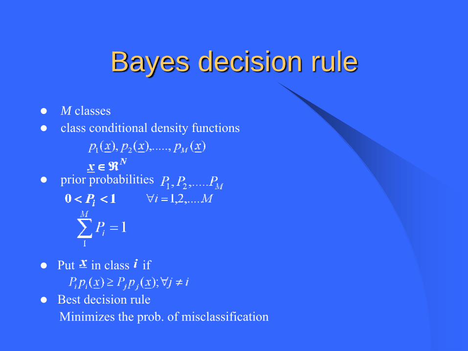
Bayes decision ruleM classesclass conditional density functions

prior probabilities

Put in class if

Best decision ruleMinimizes the prob. of misclassification

• We may not know .(Estimation of density functions), Normal distribution

• We may not know

• Error prob. may be difficult to obtain

• Other decision rules are needed

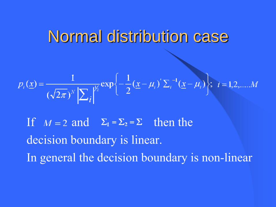
Normal distribution case

If and then the decision boundary is linear.In general the decision boundary is non-linear

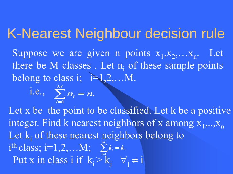
Suppose we are given n points x1,x2,…xn. Letthere be M classes . Let ni of these sample pointsbelong to class i; i=1,2,…M.

K-Nearest Neighbour decision rule

i.e.,

Let x be the point to be classified. Let k be a positiveinteger. Find k nearest neighbors of x among x1,..,xnLet ki of these nearest neighbors belong toith class; i=1,2,…M;Put x in class i if ki > kj ∀j ≠ i

Minimum distance classifier

Let μ1,μ2,…μM be the means of the M classes. Let d(a,b) denote the distance between a & b. (Examples : Euclidean, Minkowski) Put x in class i if d(x, μi) < d(x, μj) ∀j ≠ i

Some remarks

Standardization & normalizationChoosing the appropriate distance functionProbability of misclassificationCost of misclassification

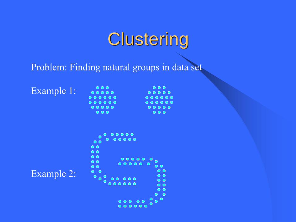
ClusteringProblem: Finding natural groups in data set

Example 1:

Example 2:

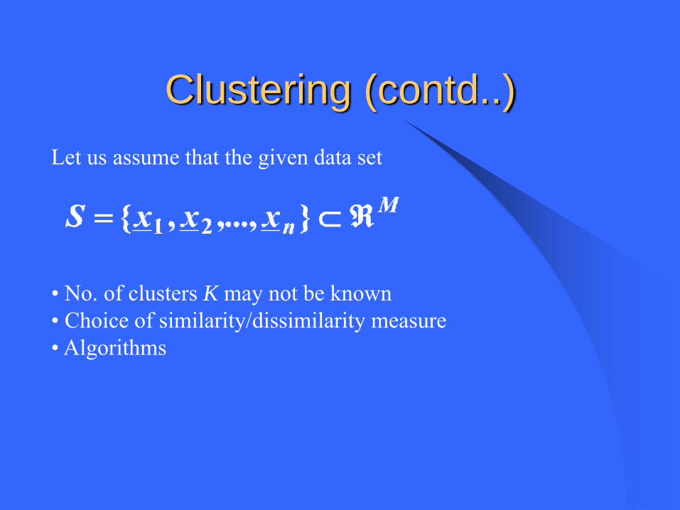
Clustering (contd..)Let us assume that the given data set

• No. of clusters K may not be known• Choice of similarity/dissimilarity measure• Algorithms

Dissimilarity Measures• Metrics

Euclidean distance

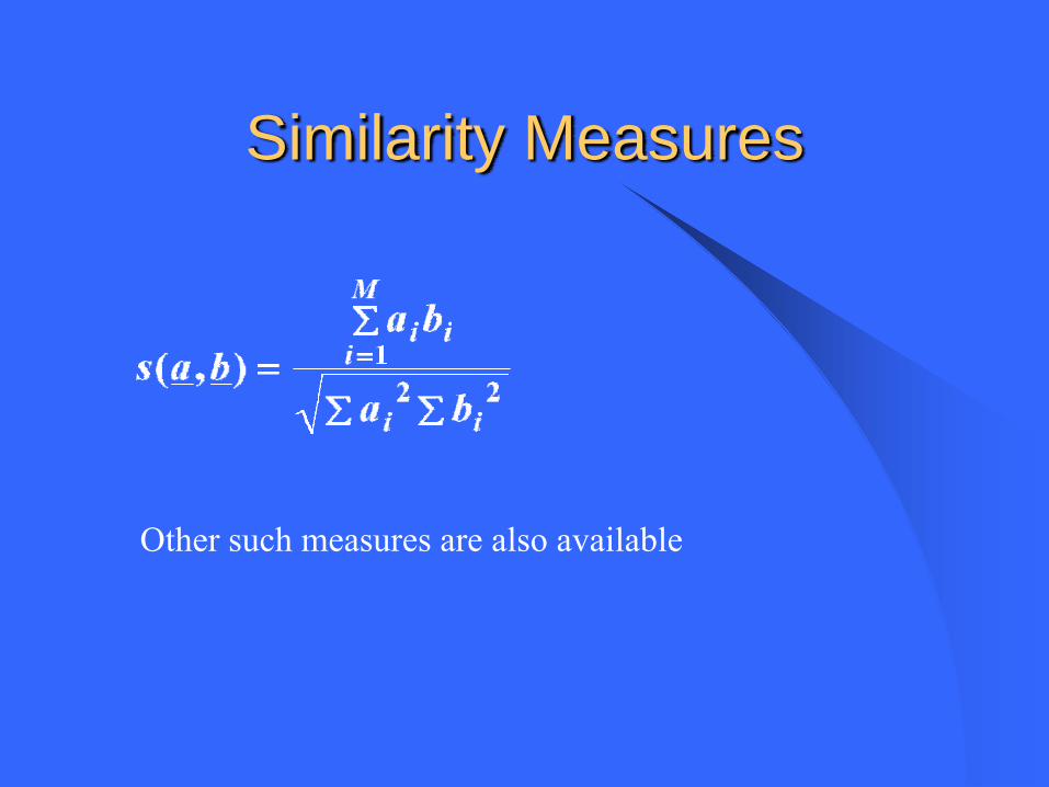
Similarity Measures

Other such measures are also available

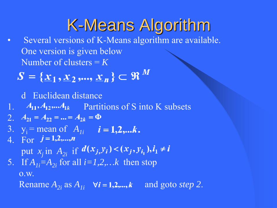
K-Means Algorithm• Several versions of K-Means algorithm are available.

One version is given belowNumber of clusters = K

d Euclidean distance 1. Partitions of S into K subsets 2.3. yi = mean of A1i4. For

put xj in A2i if 5. If A1i=A2i for all i=1,2,…k then stop

o.w.Rename A2i as A1i and goto step 2.

K-Means Algorithm (contd..)

• Number of iterations is usually decided by the user

• provides basically convex clusters

• Non convex clusters may not be obtained

• Two different initial partitions may give rise to two different clusterings

Hierarchical Clustering Techniques

• Agglomerative

• Divisive

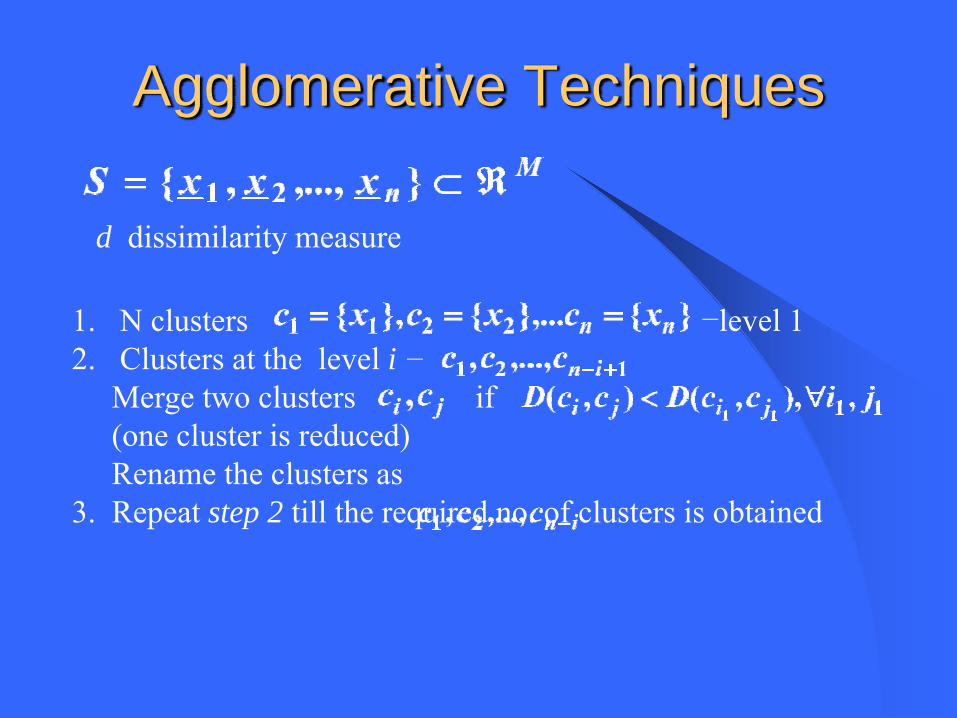
Agglomerative Techniques

1. N clusters level 12. Clusters at the level i

Merge two clusters if (one cluster is reduced)Rename the clusters as

3. Repeat step 2 till the required no. of clusters is obtained

d dissimilarity measure

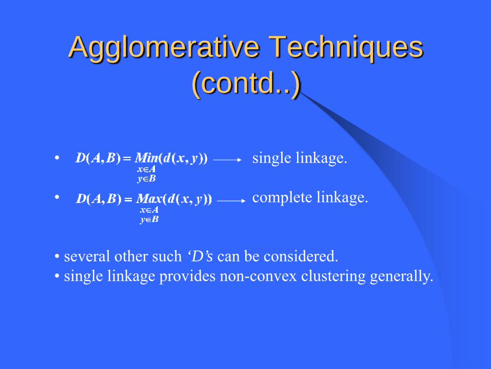
Agglomerative Techniques (contd..)

• single linkage.

• complete linkage.

• several other such ‘D’s can be considered.• single linkage provides non-convex clustering generally.

Feature selection

Feature X1, X2,…,XN

b no. of features to be selected. b < NUses :

Reduction in computational complexityRedundant features act as noise. Noise removalInsight into the classification problem.

Steps of feature selection

Objective function J which attaches a value to every subset of features is to be defined.Algorithms for feature selection are to be formulated.

Objective functions for feature selection (Devijver & Kittler)

Probabilistic separability (Chernoff, Bhattacharyya, Matusita, Divergence)Inter class distance

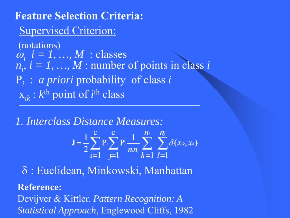
Feature Selection Criteria:Supervised Criterion:

ωi i = 1, …, M : classesni, i = 1, …, M : number of points in class iPi : a priori probability of class ixik : kth point of ith class

1. Interclass Distance Measures:

(notations)

δ : Euclidean, Minkowski, ManhattanReference:Devijver & Kittler, Pattern Recognition: A Statistical Approach, Englewood Cliffs, 1982

2. Probabilistic Separability Measures:Bhattacharyya Distance:

3. Information Theoretic Measures:Mutual Information:

Difficulty: Computing the probabilities.Empirical estimates are used.

Unsupervised Criterion:Entropy (E):Similarity between points xi and xj:

Sij = e –αδ(xi,xj) i,j = 1, …, l

Other unsupervised indices:

•Fuzzy Feature Evaluation Index•Neuro-fuzzy Feature Evaluation Index

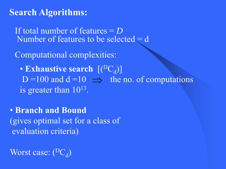
Search Algorithms:

If total number of features = D

Computational complexities:• Exhaustive search [(DCd)]D =100 and d =10 the no. of computationsis greater than 1013.

• Branch and Bound(gives optimal set for a class of evaluation criteria)

Worst case: (DCd)

Number of features to be selected = d

⇒

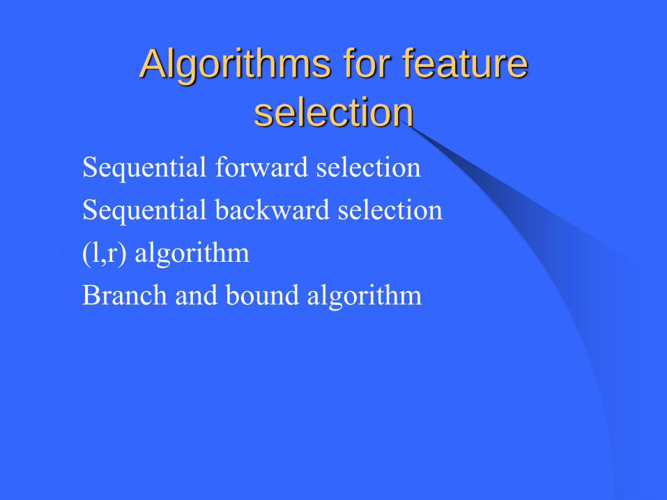
Algorithms for feature selection

Sequential forward selectionSequential backward selection(l,r) algorithmBranch and bound algorithm

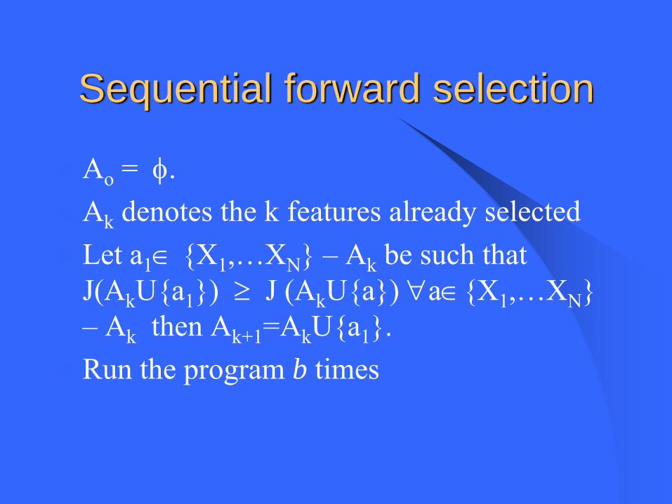
Sequential forward selection

Ao = φ.Ak denotes the k features already selectedLet a1∈ {X1,…XN} – Ak be such that J(AkU{a1}) ≥ J (AkU{a}) ∀a∈{X1,…XN} – Ak then Ak+1=AkU{a1}.Run the program b times

• Sequential Forward/Backward Search(greedy algorithms, very approximate,gives poor result on most real life data)

• Sequential Floating F/B Search (l-r algorithm)

(relatively better than SFS/SBS)

Non-Monotonicity Property:“Two best features are not always the best two”

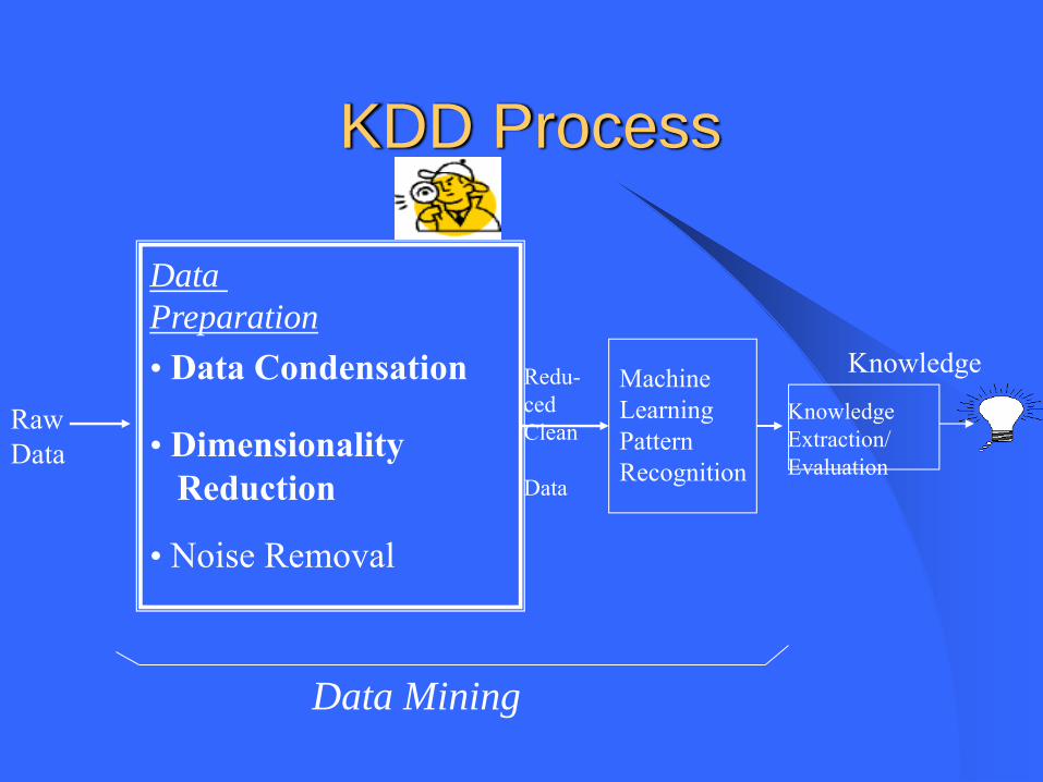
KDD Process

Data Preparation• Data Condensation

• DimensionalityReduction

• Noise Removal

MachineLearningPatternRecognition

KnowledgeExtraction/Evaluation

Redu-cedClean

Data

RawData

Data Mining

Knowledge

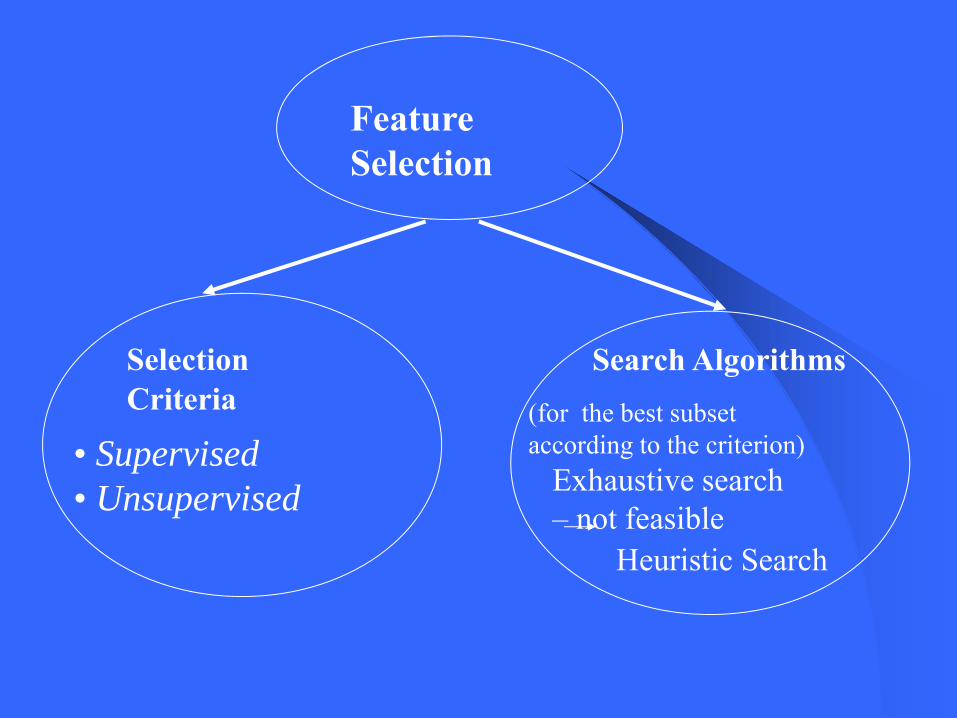
FeatureSelection

SelectionCriteria

Search Algorithms

• Supervised• Unsupervised

(for the best subset according to the criterion)

Exhaustive search – not feasible

Heuristic Search

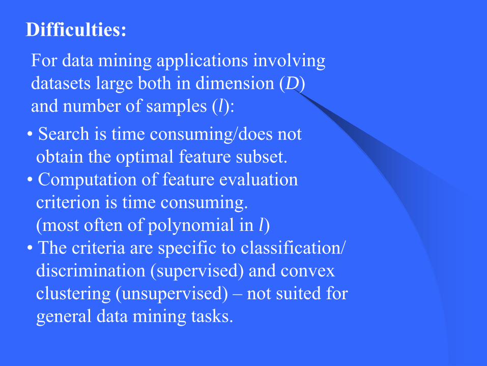
Difficulties:For data mining applications involvingdatasets large both in dimension (D)and number of samples (l): • Search is time consuming/does notobtain the optimal feature subset.

• Computation of feature evaluationcriterion is time consuming.(most often of polynomial in l)

• The criteria are specific to classification/discrimination (supervised) and convexclustering (unsupervised) – not suited forgeneral data mining tasks.

What we want !

• Algorithms not requiring search

• Easy to compute feature evaluation criterion

• More general purpose feature evaluation criteria

Principal Components

Variance covariance matrix for Find the direction in which the maximum variance occurs.Find the direction perpendicular to the earlier directions in which the maximum variance occurs.Repeat this process d times.

∑ X

Principal Components Cont..Find Eigen values of and arrange them in decreasing order

Find the normalized Eigen vectors corresponding to the Eigen values

Then are the ‘d’ principal components

∑

Dλλλλ ≥≥≥ ....321

Daaaa ,....,, 321XaXaXa d

''2

'1 ,....,

Another approach to feature selection:

Relevance, redundance: multivariate analysis

Principle: Retain relevant features, Discard redundant ones.

(Wilk’s Lambda test, canonical correlation)

Notions:

Reference:J. A. Hartigan, Clustering Algorithms,Wiley, NY, 1975

Supervised schemes:

Markov Blanket Approach:Eliminate a feature if it gives little or noadditional information beyond that givenby the other selected features.Definition 1: (Conditional Independence)Two variables A and B are said to be conditionallyindependent given some set of variables X, if for anyassignment of values a,b and x,

Pr(A=a | X=x, B=b) = Pr(A=a | X=x) Definition 2: (Markov Blanket)Let M be some set of features not containing Fi. M isa Markov blanket for Fi, if Fi is conditionally indep-endent of F-M-{Fi} given M. F is the original set.

Feature Selection Scheme:Sequentially remove the features whose Markov blanket (M) is present among the remaining features, till no more M is found. Reference:

D. Koller and M. Sahami, Towards optimalFeature selection, Proceedings Intl. Conf.On Machine Learning, 1996.

Unsupervised schemes:Independent Component Analysis:

Find out the features which are maximallyindependent.Independence of random variables:• High divergence between the joint pdfand the product of individual pdf’s.

• Maximal NonGaussianity of the jointdistribution.

Reference:M. Girolami, Advances in IndependentComponent Analysis, Springer Verlag 2000

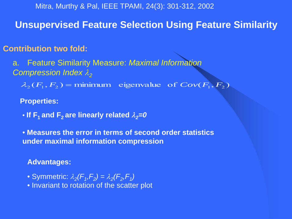
Unsupervised Feature Selection Using Feature Similarity

Mitra, Murthy & Pal, IEEE TPAMI, 24(3): 301-312, 2002

a. Feature Similarity Measure: Maximal Information Compression Index λ2

Contribution two fold:

),( of eigenvalue minimum ),( 21212 FFCovFF =λ

Properties:

• If F1 and F2 are linearly related λ2=0

• Measures the error in terms of second order statistics under maximal information compression

Advantages:

• Symmetric: λ2(F1,F2) = λ2(F2,F1)• Invariant to rotation of the scatter plot

b. Feature Clustering Algorithm:

• Identifies groups of similar features (in terms of λ2)• Selects a feature from each group• Groups are formed s.t.

• information loss is bounded• redundancy reduction is maximized

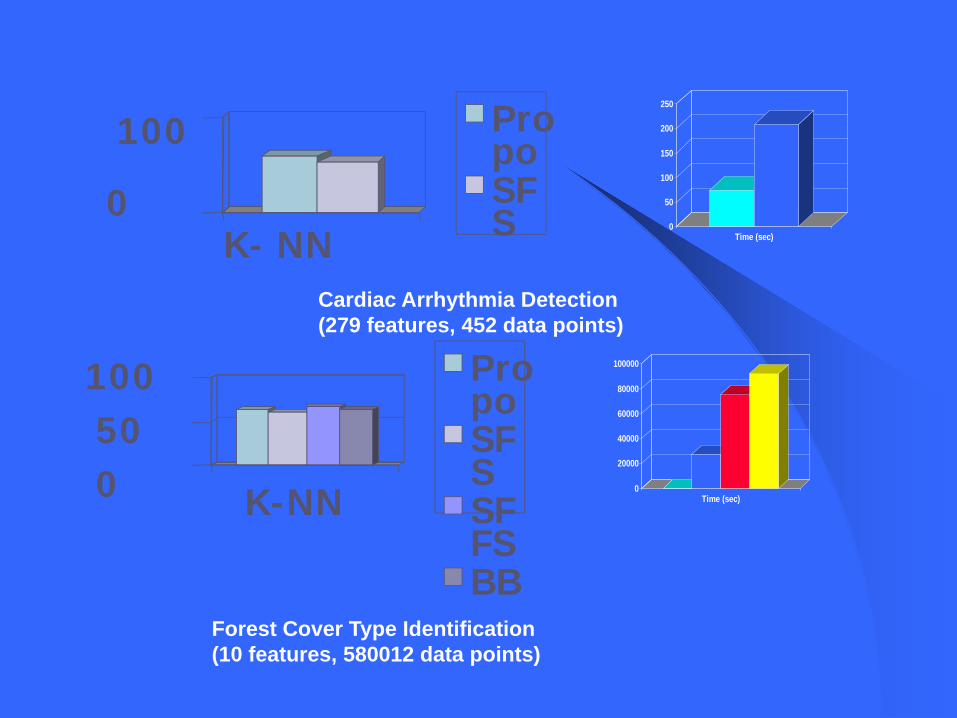
Performance and computation time

0

100

K- NN

PropoSFS 0

20000

40000

60000

80000

100000

Time (sec)

0

100

K-NN

Proposed

SFS0

50000

100000

150000

200000

250000

300000

Time (sec)

Hand Written Numeral Recognition(649 features, 5000 data points)

Speech Recognition(617 features, 7797 data points)

For a all data: Size of reduced feature set = ½ of original feature set

0

100

K- NN

PropoSFS 0

50

100

150

200

250

Time (sec)

050100

K-NN

PropoSFSSFFSBB

0

20000

40000

60000

80000

100000

Time (sec)

Cardiac Arrhythmia Detection(279 features, 452 data points)

Forest Cover Type Identification(10 features, 580012 data points)

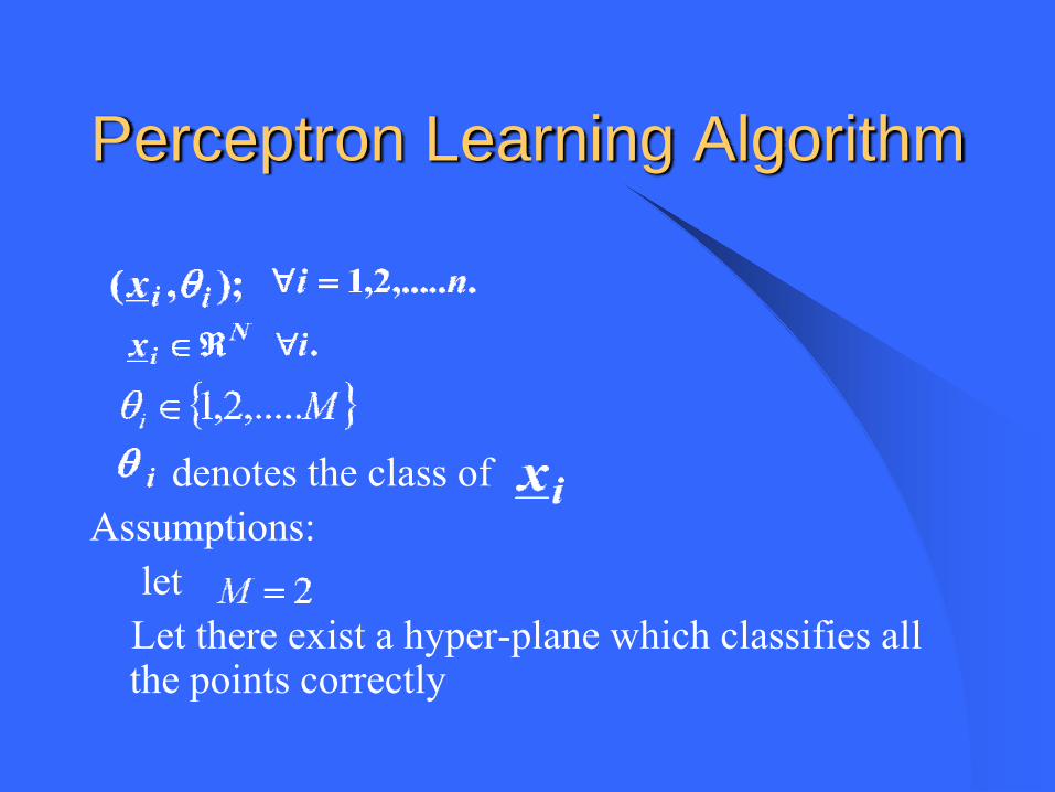
Perceptron Learning Algorithm

denotes the class of Assumptions:

let Let there exist a hyper-plane which classifies all the points correctly

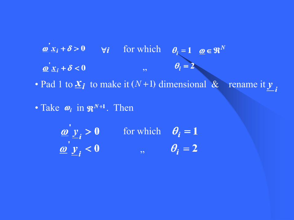
for which

”• Pad 1 to to make it dimensional & rename it

• Take in . Then

for which

”

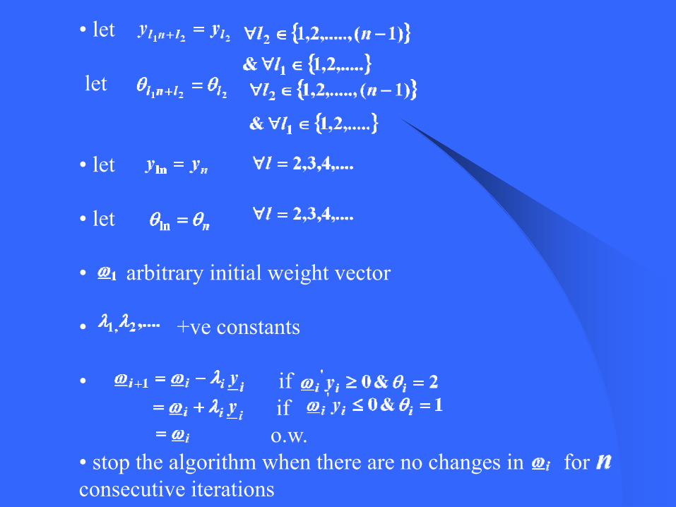
• let

let

• let

• let

• arbitrary initial weight vector

• +ve constants

• ififo.w.

• stop the algorithm when there are no changes in for consecutive iterations

• suppose and

• convergence theoremfor any arbitrary initial weight vector , andthe algorithm converges for

• hyper-plane may not be in the “middle”

• generalization capability may be weak.

Remarks

XOR ProblemIn higher dimensions, one may be able to obtain a hyper-plane separating the two classes.

Data Condensation:

• Datasets often contain redundant data.

• Replace a large dataset by a small subsetof representative patterns.

• Performance of Pattern Recognition algorithms when trained on the reduced set should be comparable to that obtained when trained on the entire dataset.

Data Condensation Algorithms:

• Problem dependent:Specific to the data mining tasks (e.g., classification, rule generation), and algorithms (e.g., Neural Network, K-NN).

• Problem independent:Not specific to any task or algorithm.

Goal: To obtain a faithful representationof the data.

Suitable for many data mining applications.

Multiscale Representation:

Multiscale representation of data refersto visualization of data at different ‘scales’where the term scale may refer to either unit, Frequency, window size, or kernel parameter.

Applications:

• Remote sensing• Geographical information systems/maps• Population census• Time series data (stock exchange/seismic)• Image/Shape retrieval/Multimedia indexing

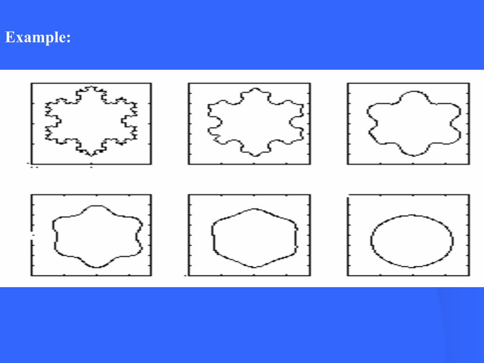
Example:

Data Condensation Methods:

Statistical Sampling:

• Random Samplingwith replacementwithout replacement

(poor result for noisy data and sparsesampling ratios)

• Stratified sampling

(weightage to weak classes)

Astrahan’s Method: (1970)

1. Select two radii d1 and d2.2. For every point in the dataset, find the

number of other points lying within d1distance of it.

3. Find the point having the highest numberof point in its d1 neighborhood.

4. Retain the above point in the reduced set.5. Discard all points from the dataset lying

within a distance d2 from the selectedpoint. Repeat till the dataset is exhausted.

Contd…..

Note:• Choices of d1, d2 are nontrivial.• Minimal spanning tree base techniquesare used.

Condensed Nearest Neighbor: (1968)1. Setup two bins Grabbag and Store.2. Select k points randomly from

the dataset and place in Store; theremaining points are placed in Grabbag.

3. Classify the points in Grabbag by k-NNrule using the points in Store.

4. Transfer the misclassified points fromGrabbag to Store.

5. Repeat over several iterations till thereare no more transfers. Use Store as thereduced dataset.

Contd….

Note:• Retains noise points in the reduced set.• To achieve noise tolerance Aha (1991)

suggests a modified version, the IB3 (Instance Based Learning) algorithm.

Learning Vector Quantization:Vector quantization: Use a set of codebookvectors to obtain a reduced representation of the data, such that squared quantization error is minimized.

LVQ1:mc: a codebook vector, x: a data pointChoose a random set of codebook vectors.

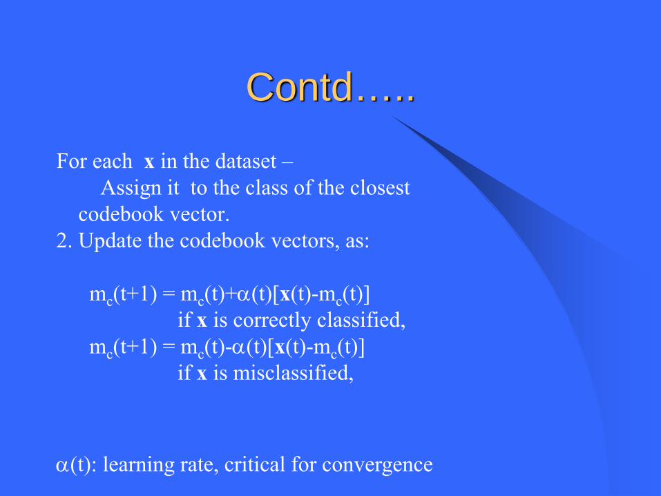
Contd…..

For each x in the dataset –1. Assign it to the class of the closest

codebook vector.2. Update the codebook vectors, as:

mc(t+1) = mc(t)+α(t)[x(t)-mc(t)]if x is correctly classified,

mc(t+1) = mc(t)-α(t)[x(t)-mc(t)]if x is misclassified,

α(t): learning rate, critical for convergence

LVQ3:More sophisticated versions of LVQ exist.

More complex update rules for codebookvectors compared to LVQ1.

Additional update rules for points lying within a window of the decision boundary.

The update rule shifts the decision boundarytowards the Bayes limit.

Reference

T. Kohonen, The Self-Organizing Map,

Proc. IEEE, Vol 78, 1990, pp 1464-1480

Locally Assymetric Metric (LASM):

1. A reduced set of random points are chosen.

2. A weight vector wi is attached to each point.

3. wi are used to compute a feature weighted metric (LASM) between two points.4. Weights wis are learned using reward

-punishment steps, till the desirableclassification accuracy is achieved.

Reference

F. Ricci and P. Avesani, Data compressionand local metrics for nearest neighborclassification. IEEE TPAMI, Vol 21, 1999pp 380-384

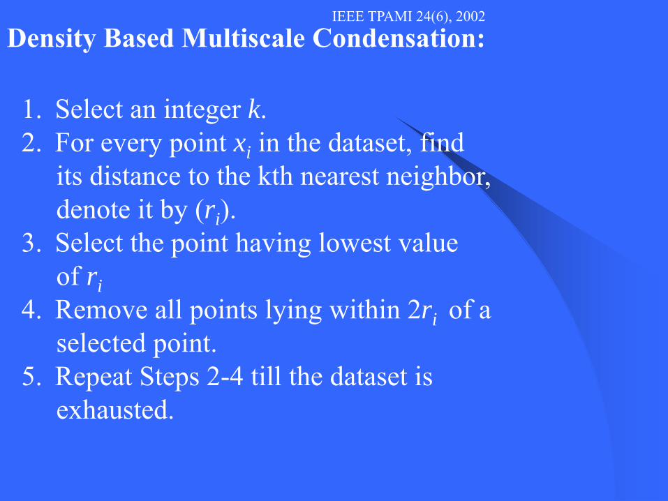
Density Based Multiscale Condensation:IEEE TPAMI 24(6), 2002

1. Select an integer k.2. For every point xi in the dataset, find

its distance to the kth nearest neighbor,denote it by (ri).

3. Select the point having lowest value of ri

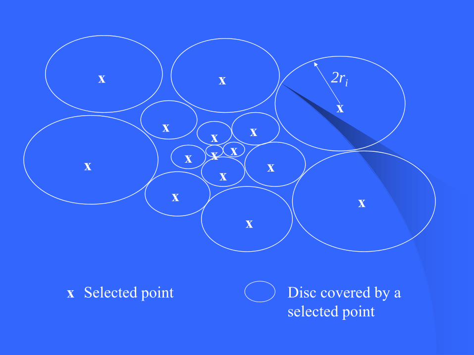
4. Remove all points lying within 2ri of a selected point.

5. Repeat Steps 2-4 till the dataset is exhausted.

xx

xx

x

x

xx

x

x x

xx

xx

x Selected point Disc covered by aselected point

2ri

Remarks:

1. Provides detailed representation ofdenser regions of feature space andlenient representation of sparser regions(multiresolution representation).

2. Based on k nearest neighbor nonparametric density estimation.

3. Different `scales’ of detail achieved byvarying value of k.

4. Does not require choice of radii d1, d2as in Astrahan’s method.

Evaluation Criteria:Goodness of reduced set is measured bythe difference of nonparametric densityestimates obtained using the original datasetand the reduced set. If g1(x) and g2(x) are the estimates, error J:

∑=

=N

ixxD

NJ

1))(2g),(1g(1 N : number of data points

)(2g)(1gln))(2g),(1g(

xxxxD =

Distance D between two distributions:Log-likelihood ratio

)(2g)(1g(x)ln2g))(2g),(1g(

xxxxD = Kullback-Liebler

information numberLower value of J denotes better representation

Datasets:Forest Covertype: (GIS data of USA)Number of samples: 580012Number of features: 10 (continuous)Number of classes: 7 (pine, fir, birch etc)Task: Classification

Satellite Image: (IRS image of Calcutta)Number of samples: 262144Number of features: 4(spectral bands 0-255)Task: Clustering

Census: (population of Los Angeles)Number of samples: 300000Number of features: 133Task: Rule GenerationMetric: Value Difference Metric (Wilson 2000)

Source:http://www.kdd.ics.uci.edu/

Contd……

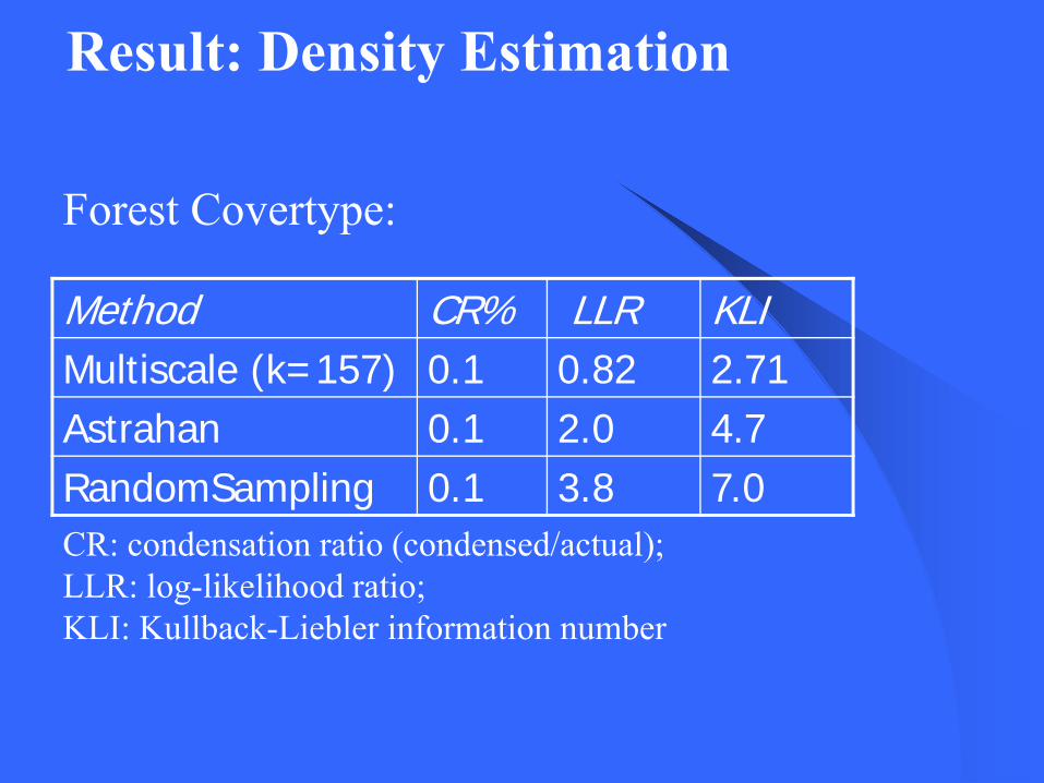
Result: Density Estimation

Method CR% LLR KLIMultiscale (k=157) 0.1 0.82 2.71Astrahan 0.1 2.0 4.7RandomSampling 0.1 3.8 7.0CR: condensation ratio (condensed/actual);LLR: log-likelihood ratio;KLI: Kullback-Liebler information number

Forest Covertype:

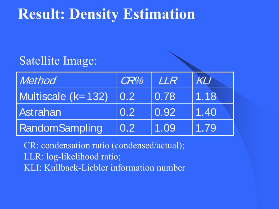
Method CR% LLR KLIMultiscale (k=132) 0.2 0.78 1.18Astrahan 0.2 0.92 1.40RandomSampling 0.2 1.09 1.79

Satellite Image:

CR: condensation ratio (condensed/actual);LLR: log-likelihood ratio;KLI: Kullback-Liebler information number

Result: Density Estimation

CR: condensation ratio (condensed/actual);LLR: log-likelihood ratio;KLI: Kullback-Liebler information number

Method CR% LLR KLIMultiscale(k=127) 0.1 0.27 1.55Astrahan 0.1 0.31 1.70RandomSampling 0.1 0.40 1.90

Census:

Result: Density Estimation

Result: Classification

Condensation Algorithm

CR% K-NN (k=11)Accuracy

MLPAccuracy

Multiscale 0.1 83.10 70.01LVQ3 0.1 75.01 68.08LASM 0.1 74.50 -Astrahan’s 0.1 66.90 59.80StratifiedSampling

0.1 44.20 36.10

RandomSampling

0.1 37.70 29.80

Forest Covertype Dataset:

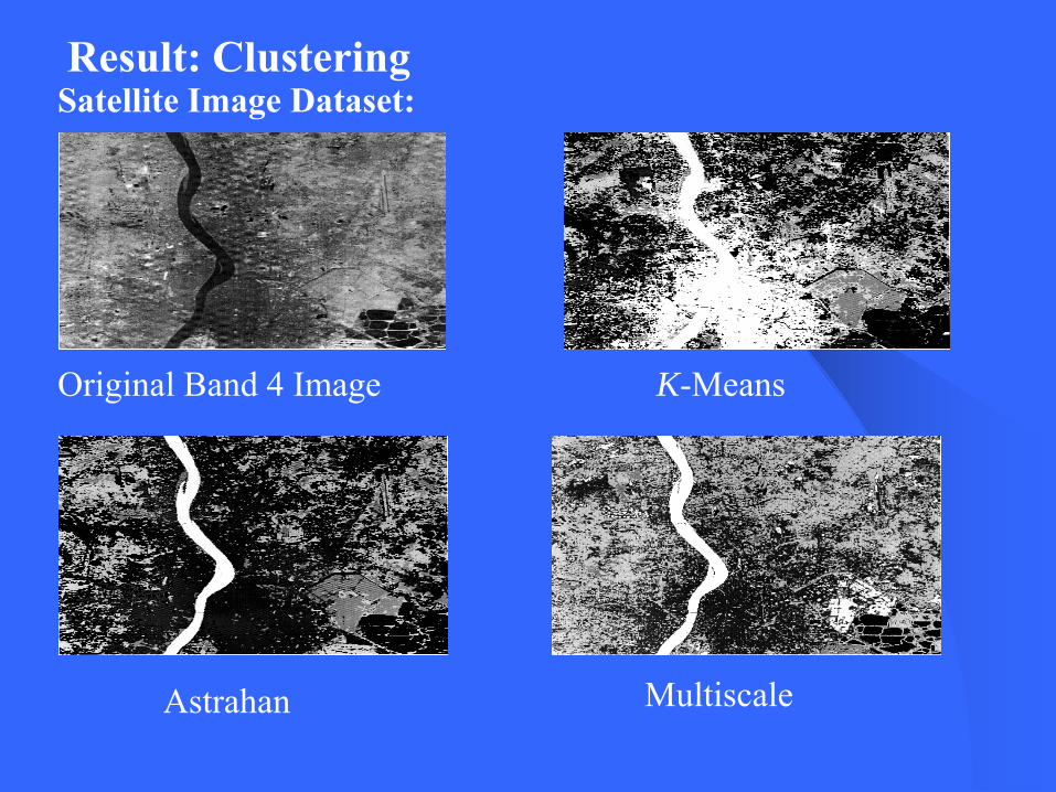
Result: ClusteringSatellite Image Dataset:

K-Means

Astrahan Multiscale

Original Band 4 Image

Result: Rule Generation using C4.5

Method CR% # of rules Accuracy UncoveredSample

RandomSampling

0.1 448 32.1% 40.0%

Stratified Sampling

0.1 305 38.8% 37.0%

CNN 0.1 270 32.0% 55.0%Astrahan 0.1 245 48.8% 25.0%Multiscale 0.1 178 55.1% 20.2%

Census Dataset:

Proposed method gives compact ruleBase with high accuracy and cover.

Thank You

Statistical Learning theorygiven

probability distribution on the datais unknown

let be the i.i.d. from suppose we have a machine whose task is to learn the mapping

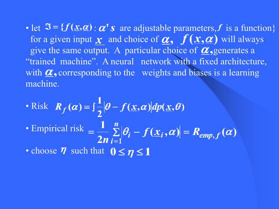
• let : are adjustable parameters, is a function}for a given input and choice of will always give the same output. A particular choice of generates a

“trained machine”. A neural network with a fixed architecture, with corresponding to the weights and biases is a learning machine.

• Risk

• Empirical risk

• choose such that

with probability

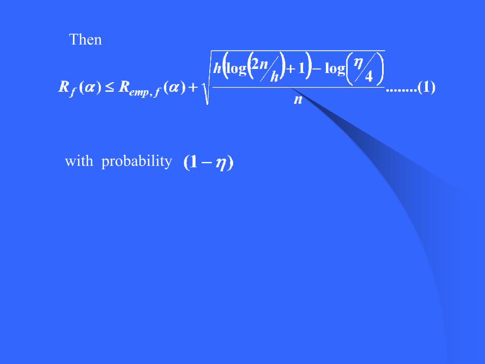
Then

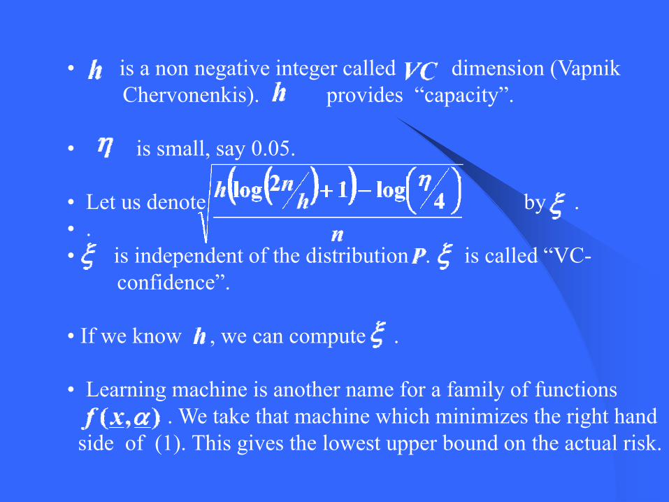
• is a non negative integer called dimension (VapnikChervonenkis). provides “capacity”.

• is small, say 0.05.

• Let us denote by . • .• is independent of the distribution . is called “VC-

confidence”.

• If we know , we can compute .

• Learning machine is another name for a family of functions. We take that machine which minimizes the right hand

side of (1). This gives the lowest upper bound on the actual risk.

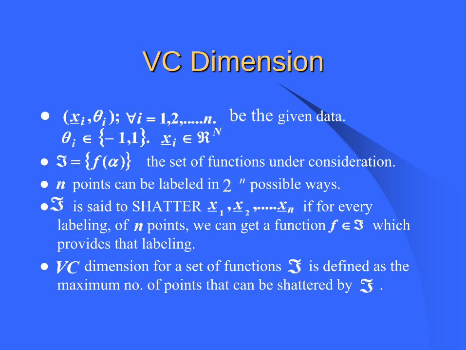
VC Dimension

be the given data.

the set of functions under consideration.points can be labeled in possible ways.is said to SHATTER if for every

labeling, of points, we can get a function which provides that labeling.

dimension for a set of functions is defined as the maximum no. of points that can be shattered by .

• dimension is there exists one set of points that can be shattered by . It is not necessarily true that every set of points is shattered by .

Oriented hyper-planes and shattering of points in

Let consists of all straight lines

• dimension of straight lines is

• Note that dimension of straight lines is not 4.So dimension is 3.

• It can be proved that dimension of hyper-planes in is .

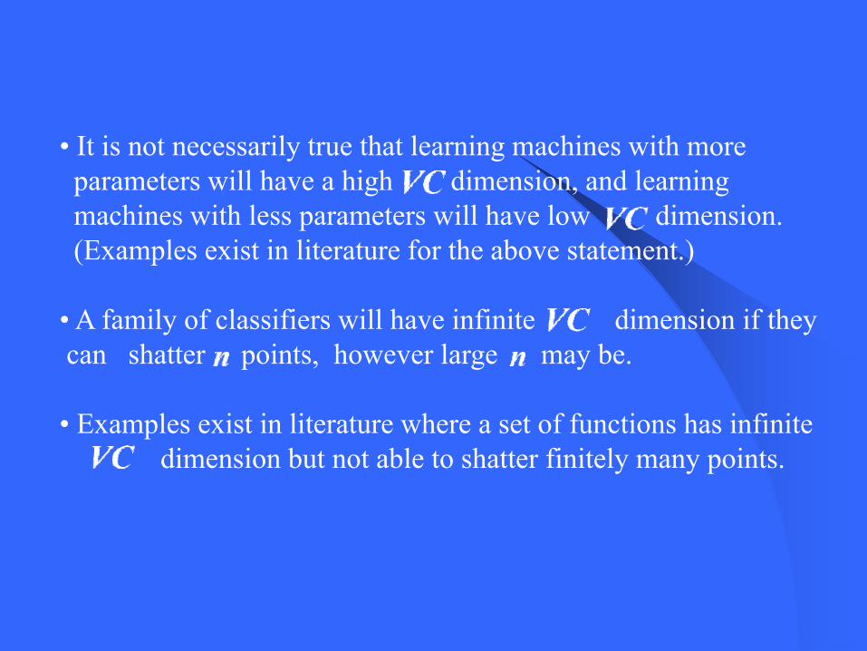
• It is not necessarily true that learning machines with more parameters will have a high dimension, and learningmachines with less parameters will have low dimension.(Examples exist in literature for the above statement.)

• A family of classifiers will have infinite dimension if they can shatter points, however large may be.

• Examples exist in literature where a set of functions has infinitedimension but not able to shatter finitely many points.

Minimization of Risk

with prob. depends on the chosen class of functions.

depend on too. Divide the entire class of functions into nested subsets

- dimension of is

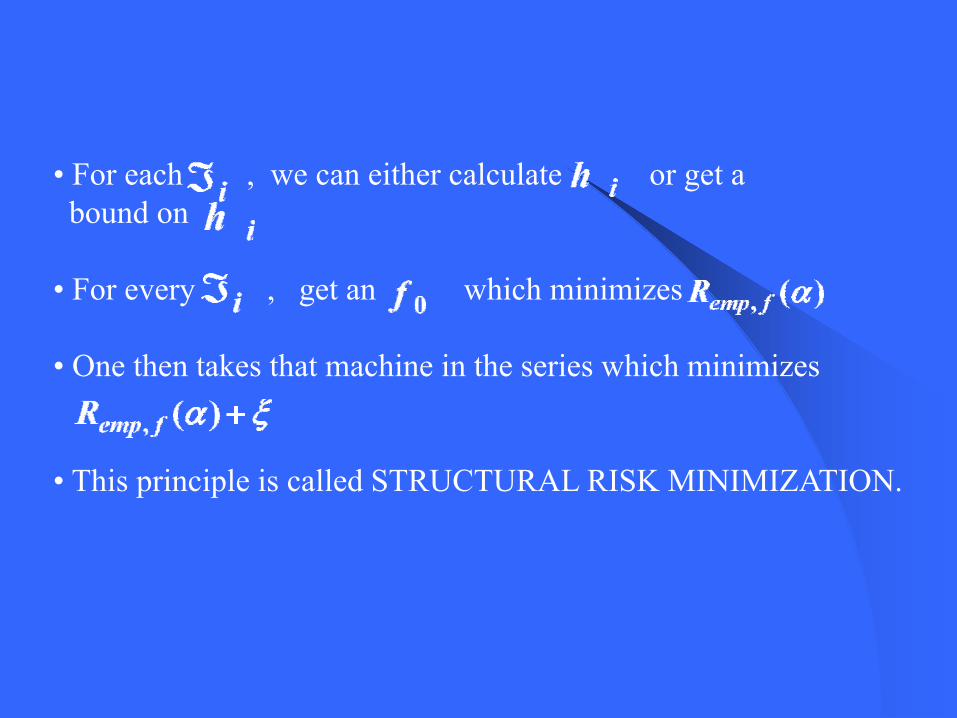
• For each , we can either calculate or get abound on

• For every , get an which minimizes

• One then takes that machine in the series which minimizes

• This principle is called STRUCTURAL RISK MINIMIZATION.

Theory connecting SVM’s to structural risk minimization principle is not dealt here.

Kernel Machines, which are advanced formulation of linear SVM’s are also not dealt here.

Maximum Margin Classifier

Data is linearly separable

i.e. Such that

for whichfor which< 0

or

If there exists one such vector for whichthen there are infinitely many such vectors.

How does one choose one optimal classifier ?

Problem Formulation

If such that then for every also satisfies

We shall set the “margin “ (min. distance of the hyper-plane to the+ve points = min distance of hyper-plane to the –ve points = 1) toone and achieve it with minimal weight

i.e. where

This is a QP problem

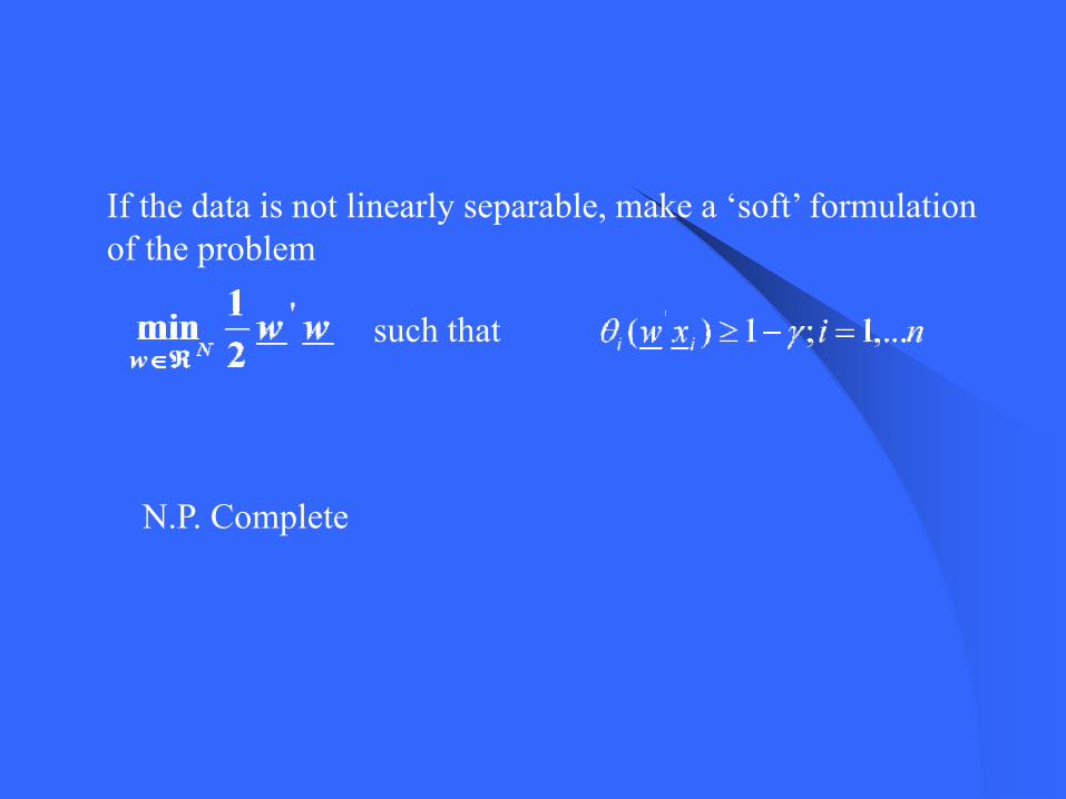
If the data is not linearly separable, make a ‘soft’ formulationof the problem

such that

N.P. Complete

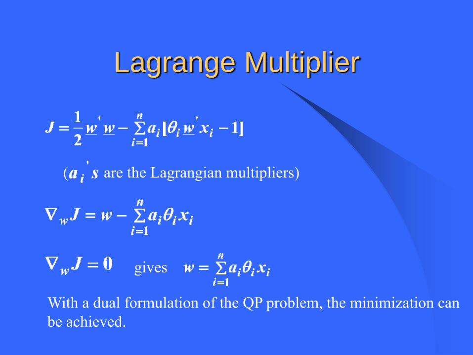
Lagrange Multiplier

( are the Lagrangian multipliers)

gives

With a dual formulation of the QP problem, the minimization canbe achieved.

References

1. S. Haykin, Neural Networks A Comprehensive Foundation, Prentice-Hall, New Jersy, 1994.2. Duda and Hart, Pattern classification and scene analysis3. Vapnik, Statistical Learning Theory

Quadratic Programming

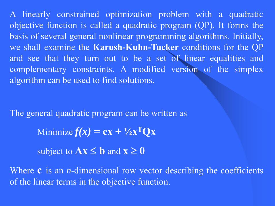
A linearly constrained optimization problem with a quadraticobjective function is called a quadratic program (QP). It forms thebasis of several general nonlinear programming algorithms. Initially,we shall examine the Karush-Kuhn-Tucker conditions for the QPand see that they turn out to be a set of linear equalities andcomplementary constraints. A modified version of the simplexalgorithm can be used to find solutions.

The general quadratic program can be written as

Minimize f(x) = cx + ½xTQx

subject to Ax ≤ b and x ≥ 0

Where c is an n-dimensional row vector describing the coefficientsof the linear terms in the objective function.

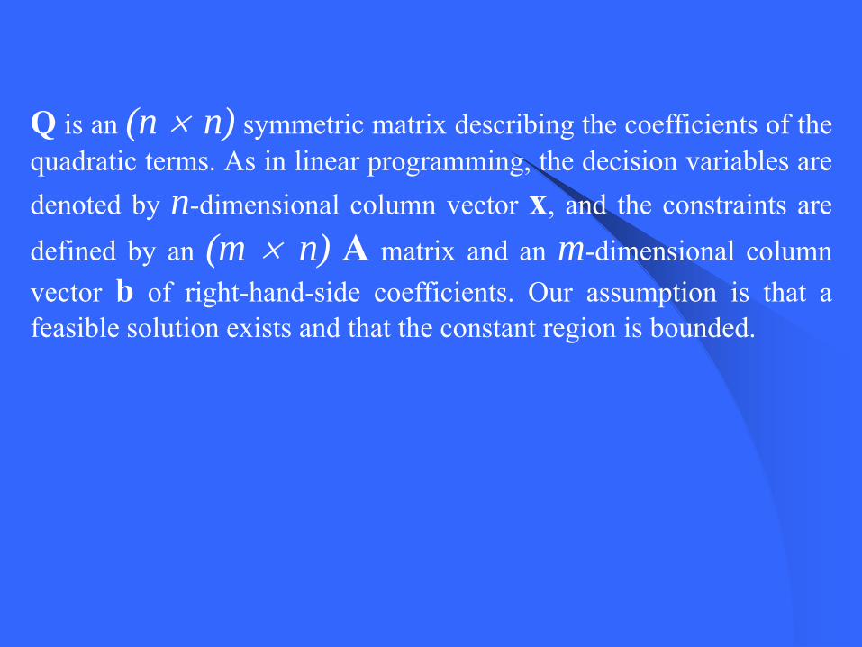
Q is an (n × n) symmetric matrix describing the coefficients of thequadratic terms. As in linear programming, the decision variables aredenoted by n-dimensional column vector x, and the constraints aredefined by an (m × n) A matrix and an m-dimensional columnvector b of right-hand-side coefficients. Our assumption is that afeasible solution exists and that the constant region is bounded.

When the objective function f(x) is strictly convexfor all feasible points the problem has a uniquelocal minimum which is also the global minimum.A sufficient condition to guarantee strictlyconvexity is for Q to be positive definite.

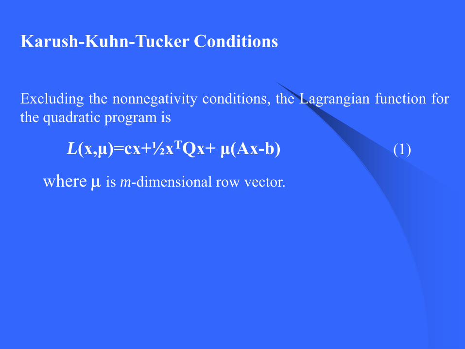
Karush-Kuhn-Tucker Conditions

Excluding the nonnegativity conditions, the Lagrangian function forthe quadratic program is

L(x,μ)=cx+½xTQx+ μ(Ax-b) (1)

where μ is m-dimensional row vector.

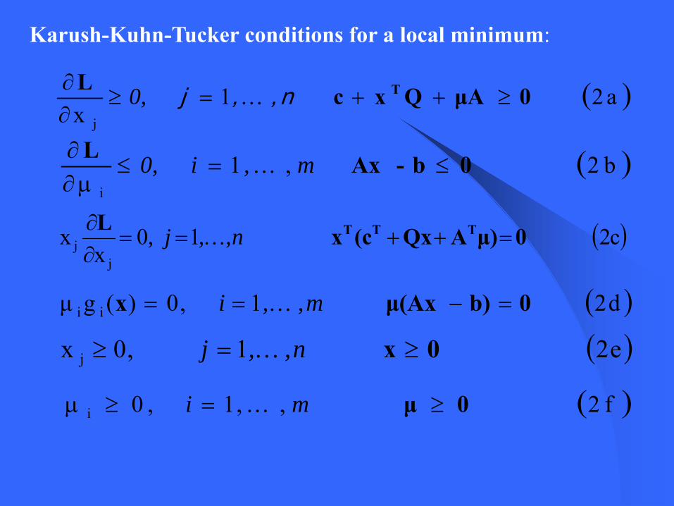
Karush-Kuhn-Tucker conditions for a local minimum:

( )f2,,1,0i m i 0μ ≥=≥μ K

( )e21,0x j n,, j 0x ≥=≥ K

( )c210x

xj

j n,, j , 0 μ)AQx(cxL TTT =++==∂∂

K

( )b2,1i

m , i 0, 0 b -Ax L≤=≤

μ∂∂

K

( )a21x j

0, 0 μA Qx cL T ≥++=≥∂∂ n,, j K

( )d21,0)(gμ ii m,, i 0 b)μ(Ax x =−== K

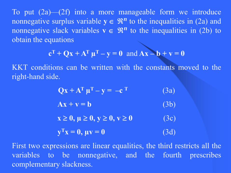
To put (2a)—(2f) into a more manageable form we introducenonnegative surplus variable y ∈ ℜn to the inequalities in (2a) andnonnegative slack variables v ∈ ℜn to the inequalities in (2b) toobtain the equations

cT + Qx + AT µT – y = 0 and Ax – b + v = 0

KKT conditions can be written with the constants moved to theright-hand side.

Qx + AT µT – y = –c T (3a)

Ax + v = b (3b)

x ≥ 0, µ ≥ 0, y ≥ 0, v ≥ 0 (3c)

yTx = 0, µv = 0 (3d)

First two expressions are linear equalities, the third restricts all thevariables to be nonnegative, and the fourth prescribescomplementary slackness.

Solving for the optimum

The simplex algorithm can be used to solve (3a) ⎯ (3d) by treatingthe complementary slackness conditions (3d) implicitly with arestricted basis entry rule. The procedure for setting up the linearprogramming model follows.

• Let the structural constraints be Eqs. (3a) and (3b) defined by theKKT conditions.

• If any of the right-hand-side values are negative, multiply thecorresponding equation by –1.

• Add an artificial variable to each equation.

•Let the objective function be the sum of the artificial variables.

• Put the resultant problem into simplex form.

The goal is to find the solution to the linear program that minimizesthe sum of the artificial variable with the additional requirement thatthe complementary slackness conditions be satisfied at each iteration.If the sum is zero, the solution will satisfy (13a) — (13d). Toaccommodate (13d), the rule for selecting the entering variable mustbe modified with the following relationships in mind.

xj and yj complementary for j= 1,…,n

μi and vi complementary for i=1,…,m

The entering variable will be the one whose reduced cost is mostnegative provided that its complementary variable is not in the basisor would leave the basis on the same iteration. At the conclusion ofthe algorithm, the vector x defines the optimal solution and thevector μ defines the optimal dual variables.

RemarksThis approach has been shown to work well when theobjective function is positive definite, and requirescomputational effort comparable to a linear programmingproblem with m + n constraints, where m is the number ofconstraints and n is the number of variables in the QP.

Conventional ML algorithms deal with input data consisting of iid samples.

Active learning systems allow the learner to make queries, which influence what data are to be added to the training set.

Active learning reduces the number of samples required by a ML algorithm, to achieve a specified accuracy level (less sample complexity)

Active Learning

Active Support Vector Learning

Class 1Class 2

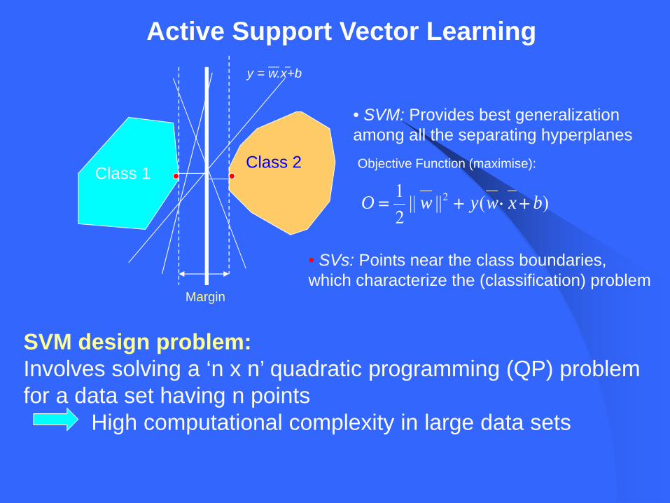
• SVM: Provides best generalizationamong all the separating hyperplanes

SVM design problem:Involves solving a ‘n x n’ quadratic programming (QP) problemfor a data set having n points

High computational complexity in large data sets

Margin

• SVs: Points near the class boundaries,which characterize the (classification) problem

Objective Function (maximise):

)( ||||21 2 bxwywO +⋅+=

y = w.x+b

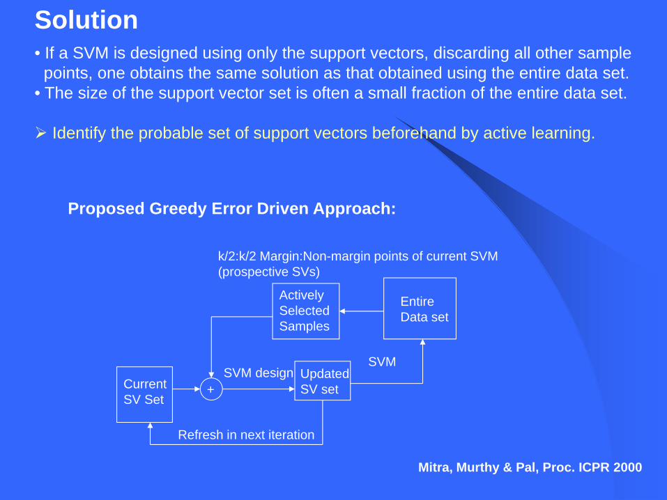
Solution• If a SVM is designed using only the support vectors, discarding all other sample points, one obtains the same solution as that obtained using the entire data set.

• The size of the support vector set is often a small fraction of the entire data set.

Identify the probable set of support vectors beforehand by active learning.

Proposed Greedy Error Driven Approach:

Mitra, Murthy & Pal, Proc. ICPR 2000

EntireData set

CurrentSV Set

+

k/2:k/2 Margin:Non-margin points of current SVM(prospective SVs)

UpdatedSV set

SVM design

Refresh in next iteration

SVM

ActivelySelectedSamples

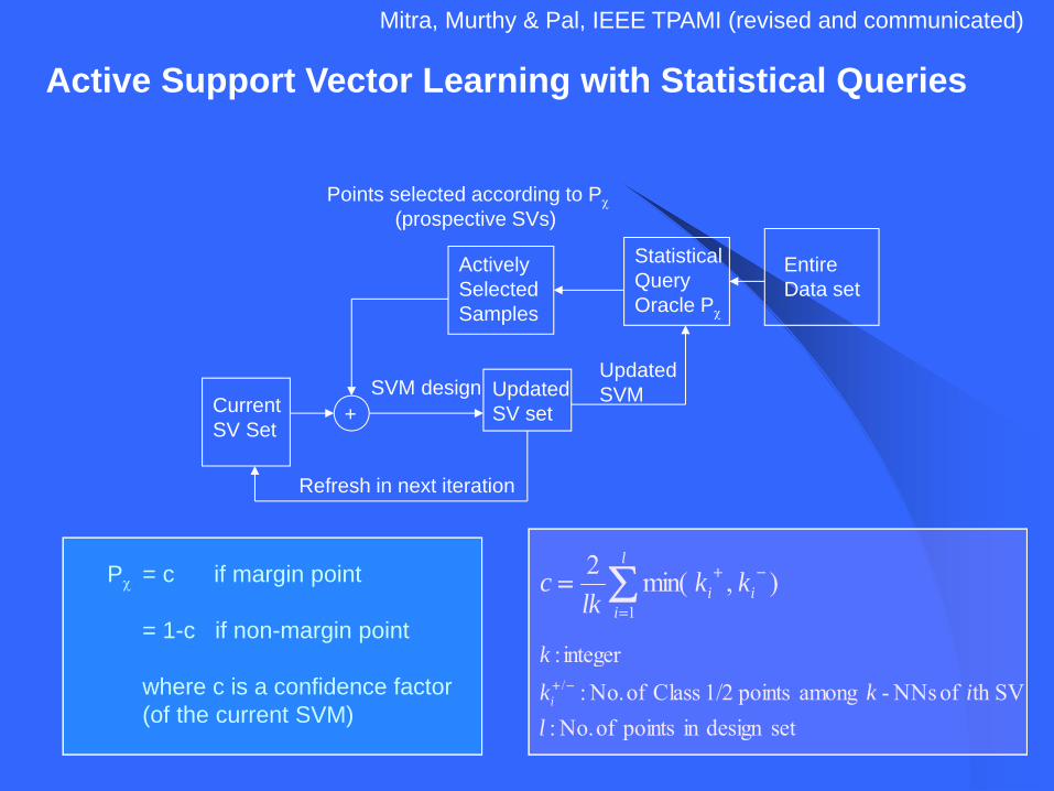
Active Support Vector Learning with Statistical Queries

Mitra, Murthy & Pal, IEEE TPAMI (revised and communicated)

EntireData set

CurrentSV Set

+

Points selected according to Pχ(prospective SVs)

UpdatedSV set

SVM design

Refresh in next iteration

UpdatedSVM

ActivelySelectedSamples

StatisticalQueryOracle Pχ

Pχ = c if margin point

= 1-c if non-margin point

where c is a confidence factor (of the current SVM)

) ,min(21

−

=

+∑= i

l

ii kk

lkc

setdesign in points of No. : SVth of NNs- among points 1/2 Class of No. :

integer:/

likk

k

i−+

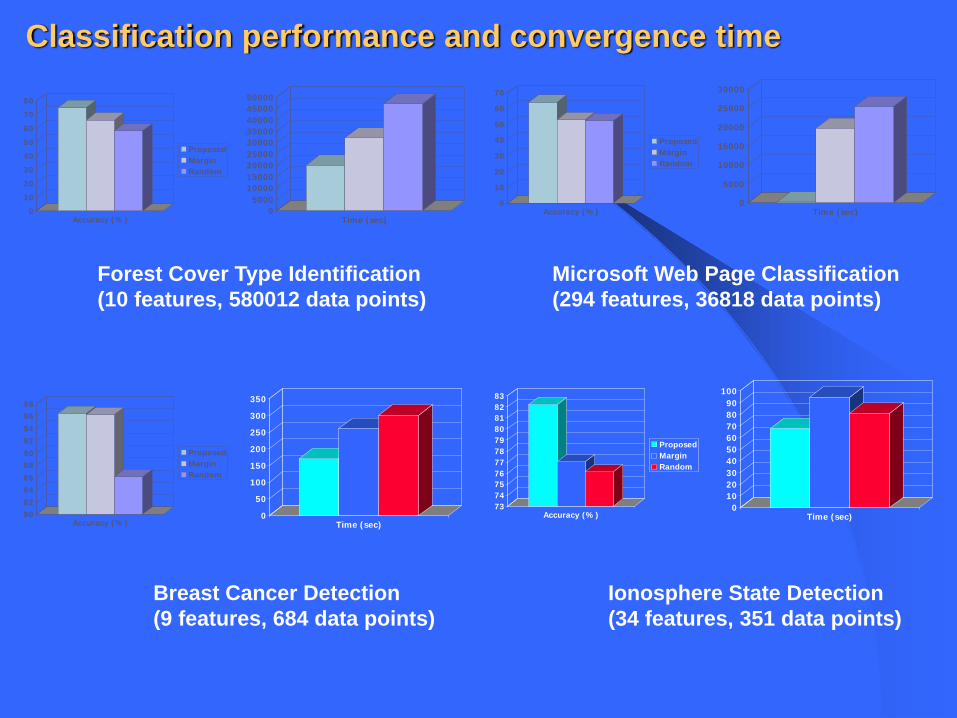
Classification performance and convergence time

0

10

20

30

40

50

60

70

80

Accuracy (%)

ProposedMarginRandom

05000

100001500020000250003000035000400004500050000

Time (sec)

0

10

20

30

40

50

60

70

Accuracy (%)

ProposedMarginRandom

0

5000

10000

15000

20000

25000

30000

Time (sec)

80828486889092949698

Accuracy (%)

ProposedMarginRandom

0

50

100

150

200

250

300

350

Time (sec)

7374757677787980818283

Accuracy (%)

ProposedMarginRandom

0102030405060708090

100

Time (sec)

Forest Cover Type Identification(10 features, 580012 data points)

Microsoft Web Page Classification(294 features, 36818 data points)

Breast Cancer Detection(9 features, 684 data points)

Ionosphere State Detection(34 features, 351 data points)

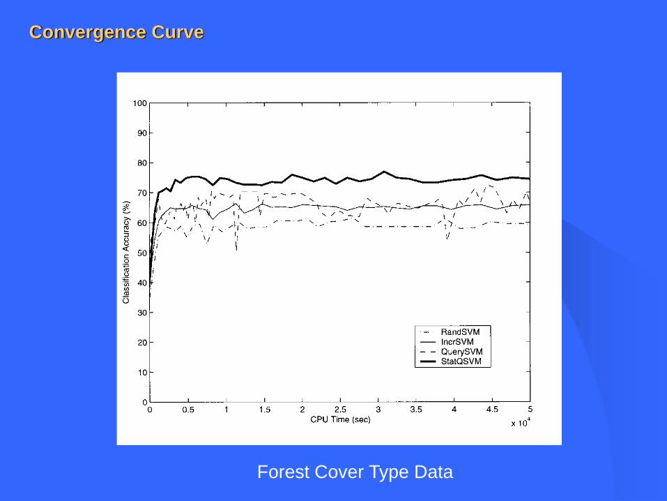
Forest Cover Type Data

Convergence Curve

• Handles the efficiency-robustness (exploration-exploitation) trade-off of an active learning system

• Fast and smooth convergence

• Margin and non-margin (interior) points • Their ratio varies adaptively with iteration depending on

the output of statistical query oracle. • More exploration in initial learning phase and more exploitation in final phase.

Unlike existing approaches which query EITHER:

• Margin points only (high exploitation) → fast but oscillatory convergence, OR• Non-margin points only (high exploration) → smooth but slow convergence

Proposed method queries BOTH:

Merits and Characteristic Features:

Thank You!!