principles of gating mechanisms of ion channels - structural
TRANSCRIPT

Principles of Gating Mechanisms of Ion Channels
Oliver Beckstein


Principles of Gating Mechanismsof Ion Channels
Oliver Beckstein
Laboratory of Molecular Biophysics andMerton College, Oxford
Michaelmas 2004
A thesis submitted in partial fulfilment of therequirements for the degree of Doctor of Philosophy at
the University of Oxford

A copy of this work has been deposited in the Bodleian Library, Oxford.Copyright c© 2004, 2005, 2007, 2008, 2012 Oliver Beckstein.First version 2005-05-29.Second version 2007-08-13 with minor corrections.Third version 2008-08-09 with minor corrections.Fourth version 2012-01-08 with minor corrections.
Viva voce examination held on 7 March 2005 by Dame Prof. Louise N. Johnson(University of Oxford) and Prof. Jean-Pierre Hansen (University of Cambridge).
This document was set in 12pt Palatino with LATEX, using KOMA-Script.It was generated with the command make thesis. See the author’shomepage http://sbcb.bioch.ox.ac.uk/users/oliver/ for electroniccopies, movies, errata, and software described in Appendix D.The title page shows the water density in the transmembrane region of thenicotinic acetylcholine receptor, which is formed by the five M2 helices. Thedensity is contoured at the bulk density. The region of broken density marksthe hydrophobic gate.
Principles of Gating Mechanisms of Ion ChannelsOliver Beckstein
Laboratory of Molecular Biophysics and Merton College, OxfordSubmitted for the degree of Doctor of Philosophy, Michaelmas 2004
AbstractIon channels such as the nicotinic acetylcholine receptor (nAChR) fulfil essen-tial roles in fast nerve transmission and cell signalling by converting an externalsignal into an ionic current, which in turn triggers further down-stream sig-nalling events in the cell. Increasing structural evidence suggests that the ac-tual mechanisms by which channels gate (i.e. switch their ion permeability) arefairly universal: Conduction pathways are either physically occluded by local-ised sidechains or the pore is narrowed by large-scale protein motions so that aconstriction lined by hydrophobic sidechains is formed. In this work the lattermechanism, termed hydrophobic gating, is investigated by atomistic computersimulations.
Simple hydrophobic model pores were constructed with dimensions estim-ated for the putative gate region of nAChR (length 0.8 nm, radius varied between0.15 nm and 1.0 nm). In long classical molecular dynamics (MD) simulations,water confined in the pore was found to oscillate between a liquid and a va-pour phase on a nano second time scale. Water would rarely permeate a poreless wide than three water molecules. A simple thermodynamic model basedon surface energies was developed, which explains the observed liquid-vapouroscillations and their dependence on pore radius and surface hydrophobicity.Similarly, Na+ ion flux is only appreciable for pore radii greater than 0.6 nm.Calculation of the free energy profile of translocating ions showed barriers topermeation of greater 10 kT for pore radii less than 0.4 nm. Comparison tocontinuum-electrostatic Poisson-Boltzmann calculations indicates that the be-haviour of the solvent, i.e. water, is crucial for a correct description of ions inapolar pores. Together, these results indicate that a hydrophobic constrictionsite can act as a hydrophobic gate.
An ongoing debate concerns the nature and position of the gate in nAChR.Based on the recent cryo-electron microscopy structure of the transmembranedomain at 4 A resolution, and using techniques established for the model pores,equilibrium densities and free energy profiles were calculated for Na+, Cl−,and water. It was found that ions would have to overcome a sizable free energybarrier of about 10 kT at a hydrophobic girdle between residues L9′ and V13′,previously implicated in gating. This suggests strongly that nAChR containsa hydrophobic gate. Furthermore, charged rings at both ends of the pore actas concentrators of ions up to about six times the bulk concentration; an effectwhich would increase the ion current in the open state. The robustness of theresults is discussed with respect to different parameter sets (force fields) and theapplied modelling procedure.


Acknowledgements
Had it not been for Mark Sansom (MSPS) and Nigel Unwin (NU) sitting ona bus from the airport to a conference location some time in 2000, you wouldread a completely different story. Something like the following conversationmust have taken place:∗
NU: “Mark, I wondered lately. The nicotinic receptor pore seems rather wide but prob-ably very hydrophobic. Do you think that this would actually be enough to keepions from going through?”
MSPS: “Hmm. . . I remember a recent paper1 where they did some simulations of wa-ter in hydrophobic, spherical cavities and said it did not stay in there.”
NU: “Interesting.”
MSPS: “Well, might be a dumb idea, but we could set up a simple pore and do someMD on it. You know, I have some motivated students coming in for a short 5month project; one of them could do it.”
NU: ”Good, let me know what comes out. . . We really need some more images to getthe resolution down. . . ”
The student was me, and the project proved to be so fruitful that I also spent thenext three years on it—thanks to Mark’s and Nigel’s insightful conversation forwhich I am very grateful to both of them.
I would also like to thank Mark Sansom for being a very supportive super-visor, who allowed me enough leeway so that I could pursue questions in struc-tural biology which were probably not strictly canonical.
Jose Faraldo-Gomez was incredibly helpful in my fledgling days as a compu-tational biophysicist; thanks to him the model pores became a reality (as muchas such a thing can become real). He masterly played the role of the advocatusdiaboli, which ensured many interesting and enjoyable discussions. I also haveto thank the members of the Sansom group, past and present, who all contrib-ute to an environment that is fun to work in. In particular Paul Barrett, KaihsuTai, and Carmen Domene, and Jeff Campbell and Jen Johnston made the lab (orthe climbing tower. . . ) a place that was not only concerned with work but alsoa place to hang out with friends. Different people were involved at differentstages of the project, and their contributions are listed on a per chapter basis:
∗Note: This conversation is reconstructed from rumours and should not be construed asfactually accurate in every detail.
vii
Confined Water I would like to thank Jose Faraldo-Gomez, Andrew Horsfield,Joanne Bright, and Peter Pohl for very interesting discussions of various aspectsof water in pores—be it imagined or real.
Hydrophobic Gating I am grateful to Paul Barrett, Kaihsu Tai, Campbell Mil-lar, Jose Faraldo-Gomez, Benoıt Roux, Nigel Unwin, and Bob Evans for theirinterest, encouragement, and readiness for critical discussions about ions andwater (again!) in toy model pores.
Ion PMFs in Model Pores This work was carried out in a very stimulatingcollaboration with Kaihsu Tai, who carried out many of the Poisson-Boltzmanncalculations. Furthermore, I would like to thank Nathan Baker for help withapbs and Born energy calculations, Graham Smith and Marc Baaden for usefuldiscussions about umbrella sampling and WHAM.
A Gate in nAChR and the α7 receptor I gratefully acknowledge discussionsin and comments from the nAChR subgroup, namely Shiva Amiri, Phil Big-gin, Andy Hung, Jennifer Johnston, and Kaihsu Tai. Shiva Amiri provided themodel of the α7 receptor. Nigel Unwin is thanked for his continuing interestand for making available their model of the transmembrane domain of TorpedonAChR prior to publication.
A Consistent Definition of Volume Ideas presented in this appendix evolvedthrough very enjoyable discussions with Andrew Horsfield during his time atthe Laboratory of Molecular Biophysics.
Funding The Wellcome Trust’s programme in Structural Biology “From Mol-ecules to Cells” generously funded my DPhil. Merton College, Oxford and theBritish Biophysical Society contributed towards travels to conferences.
However, work is not the only important thing in life, and so I am also indebtedto all the friends not mentioned yet who made these four years a great timefor me: The First Cohort (Jonathan Malo, Frank Cordes, Maria Hollerer, JohnBriggs), Werner Bar, Volker Blum, Moritz und Tina Engl, Peter Fleck, Matt Hard-ing, Markus Hormess, Tom Krieger, Carsten Kuppersbusch, Uli Lang, ThomasRechtenwald, and Zyfflich.
I’m lucky in not only having good friends but also a wonderful family. Mybrothers Nik und Chris are caring and daring company, better than anyonecould wish for. My parents, Ursula und Ernst Beckstein, gave me their never-ceasing support and love. Dafur danke ich Euch von ganzem Herzen!
Oxford, November 2004
viii

Contents
1 What is it about? 11.1 Transport through the cell membrane . . . . . . . . . . . . . . . . 11.2 Characteristics of ion channels and pores . . . . . . . . . . . . . . 31.3 Gating mechanisms . . . . . . . . . . . . . . . . . . . . . . . . . . . 4
1.3.1 Gates in ion channels . . . . . . . . . . . . . . . . . . . . . . 51.3.2 The hydrophobic gating hypothesis . . . . . . . . . . . . . 71.3.3 Water and gas channels . . . . . . . . . . . . . . . . . . . . 81.3.4 Enzyme tunnels . . . . . . . . . . . . . . . . . . . . . . . . . 9
1.4 The hydrophobic effect . . . . . . . . . . . . . . . . . . . . . . . . . 101.5 Complementing structural data . . . . . . . . . . . . . . . . . . . . 121.6 From toy models to the nicotinic receptor . . . . . . . . . . . . . . 13
2 Theory and Methods 172.1 Thermodynamics and statistical mechanics of interfaces . . . . . . 17
2.1.1 The surface tension . . . . . . . . . . . . . . . . . . . . . . . 172.1.2 Microscopic description . . . . . . . . . . . . . . . . . . . . 192.1.3 Application to computer simulations . . . . . . . . . . . . 252.1.4 Volume and other fuzzy concepts . . . . . . . . . . . . . . 28
2.2 Molecular Dynamics Simulations . . . . . . . . . . . . . . . . . . . 322.2.1 The Born-Oppenheimer approximation . . . . . . . . . . . 322.2.2 Classical Molecular Dynamics . . . . . . . . . . . . . . . . 342.2.3 Force Fields . . . . . . . . . . . . . . . . . . . . . . . . . . . 342.2.4 Algorithms . . . . . . . . . . . . . . . . . . . . . . . . . . . 40
2.3 Free energy calculations . . . . . . . . . . . . . . . . . . . . . . . . 462.3.1 The potential of mean force . . . . . . . . . . . . . . . . . . 462.3.2 Umbrella sampling . . . . . . . . . . . . . . . . . . . . . . . 482.3.3 The Weighted Histogram Analysis Method . . . . . . . . . 502.3.4 Umbrella sampling and WHAM in practice . . . . . . . . . 52
2.4 Poisson-Boltzmann electrostatics . . . . . . . . . . . . . . . . . . . 54
3 The surprising behaviour of confined water 573.1 Water in pores . . . . . . . . . . . . . . . . . . . . . . . . . . . . . . 583.2 Methods . . . . . . . . . . . . . . . . . . . . . . . . . . . . . . . . . 59
3.2.1 Model . . . . . . . . . . . . . . . . . . . . . . . . . . . . . . 603.2.2 Simulation Details . . . . . . . . . . . . . . . . . . . . . . . 61
ix

Contents
3.2.3 Analysis . . . . . . . . . . . . . . . . . . . . . . . . . . . . . 623.3 Results and Discussion . . . . . . . . . . . . . . . . . . . . . . . . . 68
3.3.1 Water near a hydrophobic surface . . . . . . . . . . . . . . 683.3.2 Water in cylindrical pores . . . . . . . . . . . . . . . . . . . 71
3.4 Conclusions . . . . . . . . . . . . . . . . . . . . . . . . . . . . . . . 83
4 Hydrophobic gating 854.1 Geometry, surface character, and local flexibility . . . . . . . . . . 854.2 Methods and Theory . . . . . . . . . . . . . . . . . . . . . . . . . . 87
4.2.1 Model . . . . . . . . . . . . . . . . . . . . . . . . . . . . . . 874.2.2 Molecular Dynamics . . . . . . . . . . . . . . . . . . . . . . 884.2.3 State based analysis . . . . . . . . . . . . . . . . . . . . . . 894.2.4 Model for liquid-vapour equilibrium in pores . . . . . . . 89
4.3 Results and Discussion . . . . . . . . . . . . . . . . . . . . . . . . . 914.3.1 Pure water . . . . . . . . . . . . . . . . . . . . . . . . . . . . 914.3.2 NaCl electrolyte . . . . . . . . . . . . . . . . . . . . . . . . . 994.3.3 Sensing external parameters . . . . . . . . . . . . . . . . . . 103
4.4 Conclusions . . . . . . . . . . . . . . . . . . . . . . . . . . . . . . . 104
5 The dielectric barrier and the hydrophobic effect 1075.1 A closer look at ions (and water) in hydrophobic pores . . . . . . 1075.2 Methods . . . . . . . . . . . . . . . . . . . . . . . . . . . . . . . . . 109
5.2.1 Molecular dynamics . . . . . . . . . . . . . . . . . . . . . . 1095.2.2 Potential of mean force . . . . . . . . . . . . . . . . . . . . . 1095.2.3 Poisson-Boltzmann calculations . . . . . . . . . . . . . . . 110
5.3 Results and Discussion . . . . . . . . . . . . . . . . . . . . . . . . . 1115.3.1 Continuum vs atomistic picture . . . . . . . . . . . . . . . . 1115.3.2 Ions in wide pores . . . . . . . . . . . . . . . . . . . . . . . 1145.3.3 Long or flexible pores . . . . . . . . . . . . . . . . . . . . . 116
5.4 Conclusions . . . . . . . . . . . . . . . . . . . . . . . . . . . . . . . 118
6 A gate in the nicotinic receptor 1216.1 The nicotinic acetylcholine receptor . . . . . . . . . . . . . . . . . . 121
6.1.1 The ligand gated ion channels . . . . . . . . . . . . . . . . 1226.1.2 Structure of the pore . . . . . . . . . . . . . . . . . . . . . . 1246.1.3 Identifying the gate . . . . . . . . . . . . . . . . . . . . . . . 128
6.2 Methods . . . . . . . . . . . . . . . . . . . . . . . . . . . . . . . . . 1286.2.1 pKa calculations . . . . . . . . . . . . . . . . . . . . . . . . . 1296.2.2 Models . . . . . . . . . . . . . . . . . . . . . . . . . . . . . . 1306.2.3 Poisson-Boltzmann calculations . . . . . . . . . . . . . . . 1316.2.4 Molecular Dynamics . . . . . . . . . . . . . . . . . . . . . . 132
6.3 Results . . . . . . . . . . . . . . . . . . . . . . . . . . . . . . . . . . 134
x
Contents
6.3.1 Protonation states . . . . . . . . . . . . . . . . . . . . . . . . 1346.3.2 Influence of the outer scaffold . . . . . . . . . . . . . . . . . 1346.3.3 Equilibrium density . . . . . . . . . . . . . . . . . . . . . . 1366.3.4 Potential of mean force . . . . . . . . . . . . . . . . . . . . . 1416.3.5 Sensitivity to the force field and backbone restraints . . . . 144
6.4 Discussion . . . . . . . . . . . . . . . . . . . . . . . . . . . . . . . . 1486.5 Conclusions . . . . . . . . . . . . . . . . . . . . . . . . . . . . . . . 151
7 Conclusions 1537.1 Water: Capillary effects at the atomic scale . . . . . . . . . . . . . . 1537.2 Ions: Dehydration barriers . . . . . . . . . . . . . . . . . . . . . . . 1547.3 A hydrophobic gate in the nicotinic receptor . . . . . . . . . . . . 1557.4 Confinement effects in other systems . . . . . . . . . . . . . . . . . 1567.5 Function follows from form . . . . . . . . . . . . . . . . . . . . . . 158
A The α7 receptor 161A.1 Methods . . . . . . . . . . . . . . . . . . . . . . . . . . . . . . . . . 161A.2 Results and Discussion . . . . . . . . . . . . . . . . . . . . . . . . . 162A.3 Conclusions . . . . . . . . . . . . . . . . . . . . . . . . . . . . . . . 164
B A consistent definition of volume at the molecular scale 165B.1 Introduction . . . . . . . . . . . . . . . . . . . . . . . . . . . . . . . 165B.2 Theory . . . . . . . . . . . . . . . . . . . . . . . . . . . . . . . . . . 166B.3 Results and Discussion . . . . . . . . . . . . . . . . . . . . . . . . . 168B.4 Conclusions . . . . . . . . . . . . . . . . . . . . . . . . . . . . . . . 171
C Analytical pore volume 173C.1 Outline of the problem . . . . . . . . . . . . . . . . . . . . . . . . . 174C.2 Calculation and Results . . . . . . . . . . . . . . . . . . . . . . . . 174C.3 Conclusions . . . . . . . . . . . . . . . . . . . . . . . . . . . . . . . 178
D Programs and scripts 179D.1 Simulation setup . . . . . . . . . . . . . . . . . . . . . . . . . . . . 179
D.1.1 pgeom . . . . . . . . . . . . . . . . . . . . . . . . . . . . . . 179D.1.2 prepumbrella.pl . . . . . . . . . . . . . . . . . . . . . . . . . 181D.1.3 prepconflist.pl . . . . . . . . . . . . . . . . . . . . . . . . . . 186
D.2 Analysis . . . . . . . . . . . . . . . . . . . . . . . . . . . . . . . . . 188D.2.1 g count . . . . . . . . . . . . . . . . . . . . . . . . . . . . . . 188D.2.2 g flux . . . . . . . . . . . . . . . . . . . . . . . . . . . . . . . 191D.2.3 g ri3Dc . . . . . . . . . . . . . . . . . . . . . . . . . . . . . . 195D.2.4 a ri3Dc . . . . . . . . . . . . . . . . . . . . . . . . . . . . . . 197D.2.5 g wham . . . . . . . . . . . . . . . . . . . . . . . . . . . . . 200
xi

Contents
D.3 Trajectory generation . . . . . . . . . . . . . . . . . . . . . . . . . . 202D.3.1 Confinement in mdrun . . . . . . . . . . . . . . . . . . . . . 202D.3.2 fakepmf . . . . . . . . . . . . . . . . . . . . . . . . . . . . . 204
E Publications 207E.1 Research articles . . . . . . . . . . . . . . . . . . . . . . . . . . . . . 207E.2 Review articles . . . . . . . . . . . . . . . . . . . . . . . . . . . . . 208
Bibliography 209
xii

List of Figures
1.1 Putative occlusion gates in ion channels . . . . . . . . . . . . . . . 61.2 Macroscopic definition of hydrophobicity . . . . . . . . . . . . . . 12
2.1 Test results for density calculations from RG . . . . . . . . . . . . . 312.2 Probability density for a harmonically restrained particle at a step
barrier . . . . . . . . . . . . . . . . . . . . . . . . . . . . . . . . . . 492.3 Umbrella sampling histograms . . . . . . . . . . . . . . . . . . . . 512.4 Test cases for the WHAM procedure . . . . . . . . . . . . . . . . . 522.5 PMF analysis: Equilibration and drift . . . . . . . . . . . . . . . . 54
3.1 Water liquid-vapour oscillations in model pores . . . . . . . . . . 593.2 Model pore system . . . . . . . . . . . . . . . . . . . . . . . . . . . 613.3 Water density near a hydrophobic surface . . . . . . . . . . . . . . 693.4 Diffusion coefficients of water near a hydrophobic surface . . . . 703.5 Trajectories of permeant water molecules . . . . . . . . . . . . . . 713.6 Density of water in hydrophobic pores . . . . . . . . . . . . . . . . 723.7 Openness—water in a hydrophobic pore . . . . . . . . . . . . . . 733.8 Radial potential of mean force of water . . . . . . . . . . . . . . . 743.9 Kinetics openclosed . . . . . . . . . . . . . . . . . . . . . . . . . . 753.10 Free energy difference between open and closed state . . . . . . . 763.11 Free energy landscape of water in pores . . . . . . . . . . . . . . . 773.12 Constrained grand potential of water in hydrophobic pores . . . . 78
4.1 Simulation system: Amphipathic pore . . . . . . . . . . . . . . . . 884.2 Liquid-vapour oscillations, with ions . . . . . . . . . . . . . . . . . 924.3 Simulation data and thermodynamic model for water in pores of
varying radius and surface character . . . . . . . . . . . . . . . . . 944.4 Influence of flexibility on the liquid-vapour equilibrium . . . . . . 954.5 Thermally broadened Lennard-Jones potential . . . . . . . . . . . 984.6 Densities of water, sodium and chloride in model pores . . . . . . 1004.7 Ionic density in the core region of hydrophobic pores . . . . . . . 1014.8 Equilibrium flux Φ0 of water and ions . . . . . . . . . . . . . . . . 1024.9 Temperature dependence of the liquid-vapour equilibrium . . . . 103
5.1 Ions in pore models . . . . . . . . . . . . . . . . . . . . . . . . . . . 1085.2 Na+ potential of mean force in hydrophobic pores . . . . . . . . . 112
xiii
List of Figures
5.3 Comparison of barrier height: PB and MD . . . . . . . . . . . . . . 1145.4 PMF profile for water . . . . . . . . . . . . . . . . . . . . . . . . . . 1155.5 Radially averaged density n(r, z) in a hydrophobic pore with ra-
dius R = 1.0 nm . . . . . . . . . . . . . . . . . . . . . . . . . . . . . 1165.6 Radial Na+ distribution function g(r) . . . . . . . . . . . . . . . . 1175.7 Water PMF in pores of varying local flexibility . . . . . . . . . . . 1185.8 PMF of a water molecule in pores of differing length . . . . . . . . 119
6.1 Sequence Logos for the ligand gated ion channels . . . . . . . . . 1236.2 Gate region of nAChR . . . . . . . . . . . . . . . . . . . . . . . . . 1256.3 Radius of nAChR TM2 pore . . . . . . . . . . . . . . . . . . . . . . 1266.4 Alignment of the nAChR M2 region . . . . . . . . . . . . . . . . . 1276.5 Structure 1OED embedded in a membrane mimetic. . . . . . . . . 1296.6 Born profile of Na+ in nAChR TM and M2 . . . . . . . . . . . . . 1366.7 Water density in nAChR . . . . . . . . . . . . . . . . . . . . . . . . 1376.8 Radial densities of 1.3 mol · l−1 NaCl solution in nAChR (OPLS-AA)1386.9 Axial density n(z) in nAChR (OPLS-AA) . . . . . . . . . . . . . . . 1396.10 3D density in the nAChR gate . . . . . . . . . . . . . . . . . . . . . 1416.11 PMF of ions and water in nAChR (OPLS-AA) . . . . . . . . . . . . 1436.12 Radial densities of 1 mol · l−1 NaCl solution in nAChR (GROMOS96)1446.13 Influence of force fields on n(z) . . . . . . . . . . . . . . . . . . . . 1456.14 PMF of ions and water in nAChR (GROMOS96) . . . . . . . . . . . 1466.15 Influence of M2 backbone restraints on the Na+ PMF . . . . . . . 1486.16 PMF of ions and water in nAChR . . . . . . . . . . . . . . . . . . . 149
A.1 α7 receptor with pore surface . . . . . . . . . . . . . . . . . . . . . 162A.2 PMF in the α7 receptor . . . . . . . . . . . . . . . . . . . . . . . . . 163
B.1 Lennard-Jones potential . . . . . . . . . . . . . . . . . . . . . . . . 166B.2 Classically allowed region for a particle in a potential. . . . . . . . 167B.3 Solvent potential energy between two LJ spheres . . . . . . . . . . 168B.4 Behaviour of the integrand in the effective volume integral . . . . 169B.5 Accessible volume in the Lennard-Jones 1D example . . . . . . . . 170
C.1 Cylindrical pore intersecting a wall atom . . . . . . . . . . . . . . 173C.2 Geometry of sphere intersected by a cylinder. . . . . . . . . . . . . 175C.3 Volume of a sphere protruding into a cylinder versus cylinder
radius . . . . . . . . . . . . . . . . . . . . . . . . . . . . . . . . . . . 177
xiv

List of Tables
2.1 Water model parameters . . . . . . . . . . . . . . . . . . . . . . . . 392.2 Ion parameters . . . . . . . . . . . . . . . . . . . . . . . . . . . . . . 40
3.1 Dynamical properties of water in hydrophobic pores . . . . . . . 793.2 Osmotic permeability coefficient p f and equilibrium flux Φ0 . . . 813.3 Comparison of different studies of water in hydrophobic pores . 82
4.1 Thermodynamic model parameters . . . . . . . . . . . . . . . . . . 934.2 RMSD of wall atoms in flexible pore models . . . . . . . . . . . . 96
6.1 Equilibrium simulations of nAChR M2 . . . . . . . . . . . . . . . . 1326.2 Umbrella sampling parameters . . . . . . . . . . . . . . . . . . . . 1336.3 Protonation states in M2 at pH 7 . . . . . . . . . . . . . . . . . . . 135
D.3 Hard coded atomic species in pgeom . . . . . . . . . . . . . . . . . 181
xv

1 What is it about?
This work is concerned with ion channels, membrane-embedded proteins whichact as facilitators of diffusive ion transport through the cell’s lipid bilayer. A de-fining characteristic of ion channel function—gating—is examined closer. Phys-ical principles are investigated that are employed by protein channels to controlthe flow of ions or water. A hypothesis is put forward to explain how someknown channels are gated. It is tested with the help of computer simulations,both in simple models and a real protein structure, the nicotinic acetylcholinereceptor.
1.1 Transport through the cell membrane
A defining step in the evolution of life on earth2,3 was the appearance of mem-branes4,5 and hence the distinction between the inside of a cell and the outsideworld.6 Life relies on the efficient progression of chemical reactions.∗ Com-partmentation through membranes greatly facilitates chemical reactions by in-creasing the concentration of reactive species in the enclosed volume, thus pro-moting higher reaction rates.7 Furthermore, the interface between water and anon-polar phase, such as lipids or polycyclic aromatic hydrocarbons, provides aunique microenvironment which accumulates organic molecules and increasestheir chemical reactivity and also helps peptides to self assemble or to foldthrough the hydrophobic effect.6 It also provides a place to anchor macromolec-ular complexes so to increase the probability of specific interactions betweenthese structures and between the complexes and membrane-associated sub-strates.4 Although only measuring about 3 nm in thickness, the phospholipidbilayer provides a formidable permeability barrier to ionic species such as pro-tons or sodium ions. All organisms either use a proton or a Na+ gradient acrossthe membrane (or both) to store free energy and to drive the production of ATP.8
But the tight boundary that a membrane provides has also got its drawbacks asit almost completely abolishes the influx of vital ionic nutrients (such as aminoacids, nucleotides, and phosphate) or the efflux of toxic waste products. Thepermeability barrier is so high that only a few solute ions per minute will crossthe lipid bilayer. On the other hand, a growing bacterial cell can and must
∗Here life is viewed as a spatially confined network of chemical and physical processeswhich harnesses free energy from the surroundings to promote its replication and integrity.
1
1 What is it about?
take up millions of nutrient solute molecules per minute.4 This task requiresthe help of specialised membrane proteins which facilitate transport across themembrane.7 Broadly, they can be categorised in two groups: passive channels orpores and active carriers. Active transporters use a source of free energy to movea solute against the electro-chemical gradient; if they use another concentrationgradient as their source they are termed co-transporters, if they use chemical en-ergy they are called pumps (for instance, protons are actively pumped out of thecytosol∗ using either chemical energy from the breakdown of nutrients or theenergy of sunlight). Channels and pores facilitate transport down the electro-chemical or osmotic gradient by providing a permeation pathway through themembrane. Lastly, some solutes such as hydrophobic or lipophilic molecules orwater can also simply diffuse through the membrane.7,9
This is, however, not the whole story. For instance, if fast water transport isrequired in a cell (as for example in the kidney) specialised water channels areexpressed in the tissue, which allow water to cross the cell membrane muchfaster than by diffusion.10,11 Organisms have evolved to such a degree that anyprocess that is crucial for the functioning of the cell is catalysed by a specificprotein, including “simple” transport phenomena. Instead of relying on ran-dom diffusion, proteins evolved to speed up very specific processes such as thepermeation of Na+ ions or water through the membrane.
How do membrane proteins shape these transport processes? The questionis a complicated one and here we will confine ourselves to passive transport (orassisted diffusion) of ions and water, i.e. the proteins of interest are ion chan-nels12 and—to a lesser degree—water pores.11,13 Biochemical and biophysicalmethods have contributed greatly to our understanding in this area. But inprinciple much of the function of a protein is already implicitly laid out in itsgene sequence. The nascent peptide chain folds into its three dimensional struc-ture which determines its function. So it should be possible to understand theworking of transport proteins from the knowledge of the positions of the atomsthat make up the protein. The total number of protein structures in the proteindata bank14 has reached 27761 (October 2004) of which 86 are unique mem-brane proteins, though including only eight ion channel structures.15 The firstatomically-detailed protein structure of an ion channel was only published in1998,16 which for the first time enabled the explanation of the characteristics ofion transport in terms of the structural features.
∗It is suggested that the direction of the proton gradient reflects the conditions faced onearth by the earliest organisms before ca. 3.9 Gyr.6,8 The primordial oceans were probably acidicas are the environments near today’s deep-ocean geothermal vents, which are considered aspossible cradles of life.2 Hence a proton gradient could be established by extruding protonsand increasing the cytosol’s pH to a neutral value. Modern eukaryotic cells still maintain aneutral cytosol but pump protons across the thylakoid membrane into chloroplasts (in plants)or mitochondria (in animals).8
2

1.2 Characteristics of ion channels and pores
1.2 Characteristics of ion channels and pores
It is now known that ion channels and water pores are proteins or protein as-semblies which form an aqueous pore through the membrane.12 These passivetransport systems share three key properties.12,17
Conductivity They conduct the permeant species at very high rates (> 106 s−1
for ions and about 109 s−1 for water), typically comparable to the diffusion ratein free solution. The rate is not stoicheiometrically coupled to the consumptionof energy in the form of e.g. ATP; the permeators follow the electro-chemicalor osmotic gradient. Rapid transport of ions is required, for instance, in theconduction of nerve impulses, both in nerve and muscle cells.
Selectivity Channels typically do not conduct all solutes at the same rate, theyare selective for one particular one or a certain class. This is necessary so thatdifferent metabolic or signalling pathways can be regulated independently. Forexample, potassium channels discriminate between K+ and Na+ ions with anaccuracy of 1 000 : 1 or better12 and most channels are permeable for eithercations or anions. Some water pores (aquaporins) are only permeable for watermolecules but not for protons or other ions.11,13
Gating Lastly, all known channels can be regulated. An external signal de-termines if the channel is open so that e.g. ions can pass through, or if it isclosed, which prevents the flow of ions. This property is termed gating. The sig-nal can be the binding of a ligand to the channel∗ as, for instance, in the familyof the ligand gated ion channels,12,18 a change in the transmembrane potential(the voltage gated ion channels12,19), a change in pressure (the mechanosensit-ive channels20), or temperature (members of the transient receptor potential(TRP) channel family21). The gate is the region of the channel which preventsthe permeant species to diffuse through the pore in the closed state. Gate andsensor (the region of the channel where the signal is detected, e.g. the pocketthat binds a ligand) do not have to be close to each other. It is rather typical thatthey lie in completely different domains, often many nanometres apart.† Gatingis often meant to entail the whole sequence of actions, from sensing the signal∗Ligands can come in various shapes, e.g. neuro transmitters such as acetylcholine (ACh) or
γ-aminobutyric acid (GABA) or general cell signalling molecules (cyclic adenosine monophos-phate (cAMP), or calcium ions); in particular if the ligands are protons (H+) then the channel issaid to be proton- or pH-gated.†A general organising principle of proteins, especially of eukaryotic ones, is a division in
separate domains. Domains can evolve independently, being able to carry out very differenttasks. When these domains (or rather, their sequences) are combined, a new protein can emergewhich combines the functions of the separate building blocks.
3
1 What is it about?
(e.g. binding of a ligand), through the transduction of the signal across the pro-tein, to the structural change which opens the gate. A typical gating processtakes at least about 1 ms (in fast synaptic transmission).
We would like to understand what happens during gating, and how it de-pends on the structure of the channel. Gated ion channels are responsible forfast synaptic transmission in the central nervous system and the neuro-muscularjunction, and sensory perception of taste, temperature, and pressure,12 so know-ledge about these “switches” will contribute to our understanding of phenom-ena as diverse as muscle control, consciousness,22,23 hearing, tasting and feel-ing.21,24 Furthermore, some hereditary diseases can be traced back to mutationsthat affect channel gating, for instance, slow or fast channel syndrome, a form ofcongenital myasthenia (hereditary muscle weakness), or nocturnal frontal lobeepilepsy.25
1.3 Gating mechanisms
The gate creates a barrier to permeation. Gating—the process of opening orclosing the transmembrane pore—has at its the core the temporary removal orestablishing of this permeation barrier. If we want to understand the very com-plicated process of gating then we first need to understand where the gate islocated and how the permeators are prevented from passing through the gate.These two questions define what we mean by the term gating mechanism.
It would seem that the location of a gate is easily pinpointed, once the struc-ture of a channel is solved at atomic resolution by X-ray protein crystallography(PX) or cryo electron microscopy (cryo-EM). Ideally, one would require twohigh resolution structures, one in the functionally open state, the other in theclosed state. Then comparison might identify regions along the pore whichchanged, and by definition, the gate is a region that changes so that the chan-nel conducts. But even this ideal case (which has not been realised althoughJiang et al.26 argue that the structures of KcsA27 and MthK28 are essentially theclosed and open state of potassium channels) is not free from ambiguities. If theconformational changes are large then it might be difficult to identify a partic-ular region as “the” gate—or could a gate possibly span the whole conductionpathway? Furthermore, a crystal structure is a static snapshot of a dynamicalprotein. It could be captured in a non-physiological state, or dynamical side-chain motions might be required during conduction, which cannot be seen inthe structure. In the absence of two structures a closed state structure might stillindicate a region of, for instance, most narrow constriction, which one mightwant to identify with the gate.
The last paragraph should have made clear that an idea of what constitutesa gate is required, even if all the structural evidence is available. For example,
4

1.3 Gating mechanisms
Hille12 considers twelve theoretical models for gates but only two seem to berealised in the channel structures available so far: steric occlusion through lar-ger scale protein motions and blockage of a constriction site by a single side-chain. However, the case of steric occlusion is already ambiguous, as the fol-lowing discussion of gates in ion channels will show.
1.3.1 Gates in ion channels
Since 1998 (Ref. 16) only a handful of channel structures have been published atatomic resolution, i.e. a resolution which allows identification of the sidechains(typically, better than 4 A). All of the channels solved by X-ray crystallographyare of prokaryotic or archaeal origin because their eukaryotic homologues areinherently difficult to crystallise. The structure of the electric ray Torpedo mar-morata nicotinic acetylcholine receptor, solved by cryo-EM,29 is the only euk-aryotic membrane channel structure available. Generally, it is tacitly assumedthat bacterial channel structures also illuminate the function of the homologouseukaryotic channels. The case of the ClC chloride channels, however, suggestssome caution in this respect. The ClC structure from Salmonella enterica ser-ovar typhimurium (StClC, 3.0 A resolution30) and Escherichia coli (EcClC, 2.5 A,Ref. 31) was later shown to belong to a Cl−/H+ exchange transporter32 whereasthe mammalian homologue is a true channel.
Local sidechain block ClC channels can be gated by pH and by voltage.33
The EcClC structure suggests that a conserved glutamate residue competes withCl− ions at anion-binding site in the pore.31,34 At low pH the glutamate carboxylgroup is protonated so that the electrostatic interaction at the binding site fa-vours Cl− and hence the gate opens. Another example of local sidechain block-ing is conjectured in the outer membrane35–37 protein A (OmpA, PX at 2.5 A,Ref. 38). An arginine residue can alternatively form a salt bridge across the porein the closed state, or to a neighbouring glutamate, thus opening the pore.39
A similar “electrostatic switch” mechanism might operate in the annexins,40 afamily of calcium-dependent phospholipid-binding proteins with ion channelactivity.
Large scale steric occlusion For the channels to be discussed in the fol-lowing paragraphs there is generally evidence that opening the putative gaterequires some larger scale motion such as bending or twisting of pore liningα-helices45 or large, iris-like reconfiguration of the whole channel.46 Hence thediscussion will focus on the pore radius in the closed state. The pore radius Ris important because for a first approximation one can assume that an ion willnot penetrate a pore whose radius is smaller than the ionic radius. Bare ionic
5

1 What is it about?
nAChR
MscSKirBac1.1 MscL
Figure 1.1: Putative occlusion gates in selected ion channels. The approximate positionof the membrane is indicated by the black line. The cytosol is at the bottom of the figure.The surface of the pore is rendered within the secondary structure cartoon representa-tion of each channel. One subunit was omitted to allow a view into the constriction site(boxed in yellow), which is formed by hydrophobic residues. Pore radius in the con-striction: KirBac1.1 0.05 nm, MscL 0.16 nm, nAChR 0.31 nm (model of the α7 receptorfrom Amiri et al.41), MscS 0.32 nm. (Pore surface calculated with hole,42 images createdwith vmd43 and rendered with Raster3D44)
Pauling radii range from about 0.1 nm for small cations (0.095 nm for Na+ and0.133 nm for K+) to almost 0.2 nm for larger anions (0.181 nm for Cl−)12 withthe typical radius of a water molecule, rw = 0.14 nm, occupying an intermediateposition.47
The bacterial potassium channel KirBac1.1 (3.65 A, Ref. 48) was crystallisedin the closed state and the gate was identified at a constriction (formed byphenylalanines) where the pore radius drops to 0.05 nm (see Fig. 1.1). The KcsAchannel (2.0 A, Ref. 27), which is generally believed to be a closed state structure(especially when compared to the clearly open structure of the related MthKchannel28), displays a pore of minimum radius 0.12 nm.∗ The constriction site
∗The selectivity filter region has a minimum radius of 0.05 nm but the filter is known not toparticipate in gating. Furthermore, the filter interacts with K+ ions in a very specific manner,27
which is the basis of its selectivity.49 See also the discussion of the K-channel filter vs. the
6

1.3 Gating mechanisms
is formed by one valine sidechain from each of the four monomers. The po-tassium channels are believed to open through a bending motion of the porelining α-helices at a conserved glycine “hinge”.26,50
A second class of gated channels comprises the mechanosensitive channelsof large (MscL) and small (MscS) conductance. MscL (3.5 A, Ref. 51) appearsto have two gates: The narrow R < 0.05 nm S1 gate at the intracellular sideand a second gate (R = 0.16 nm) at the centre of the membrane, formed by astretch of hydrophobic residues such as valine and leucine.46,52–54 It turns outthat the S1 gate is not a proper gate as it leaks ions46 so the real gate is formed bythe hydrophobic constriction. The situation is less clear for MscS (3.9 A, Ref. 55).Originally, it was suggested that the structure is captured in the open state55 be-cause the prominent constriction site, formed by two rings of leucine residues,opened to a radius of about 0.32 nm. The classification as open, however, wasonly based on a rough conductance estimate and not confirmed by any othermethod.∗ The mechanosensitive channels are believed to open by a large scalemotion of the α-helical segments in an iris-like expansion.20,46,54,57
The structure of the transmembrane domain of the closed nicotinic acetylcholinereceptor (nAChR) was solved by cryo-EM to about 4 A resolution.29 The openstate structure is not known at atomic resolution but the 9 A structure58 clearlyshows a wide (R ≈ 0.65 nm) aqueous pore. The minimum constriction in theclosed state is still rather wide with R = 0.31 nm. Based on the radius, thephysiologically closed pore appears to belong to an open channel. Comparingthe two structures reveals that the pores not only differ in radius but also inthe residues which line the constriction. The constriction of the closed state isformed by a hydrophobic girdle of conserved valines or leucines. On opening,the α-helices, which line the pore, probably twist slightly so to move the valinesout of the pore and expose the polar peptide backbone to the pore lumen.59–61
1.3.2 The hydrophobic gating hypothesis
A common theme in the putative gates discussed so far is the presence of hy-drophobic residues in the constriction site. Furthermore, the nAChR gate and theMscS gate (if the structure is indeed captured in a closed state) can be hardlydescribed as occluded. With R = 0.3 nm the pore is wide enough to allowthe concurrent passage of three water molecules (r = 0.14 nm) or of a cationwith half of its solvation shell intact. It seems likely that the chemical character ofthe pore wall contributes significantly to creating a barrier for ion permeation.
nicotinic receptor hydrophobic girdle in Section 6.1.2.∗Subsequently, Anishkin and Sukharev56 argued for a closed state for reasons to be dis-
cussed in the following pages (see in particular Section 6.3.3 on page 136 and the footnote onpage 137).
7

1 What is it about?
Motivated by the structural evidence we posed the hydrophobic gating hypo-thesis:62
A gate in an ion channel can be formed by a constriction site, formedby hydrophobic sidechains such as valine, leucine, isoleucine or phenylalan-ine. The constriction need not be narrower than about 0.3 nm in ra-dius because this is already sufficient to require partial dehydration ofthe permeant ion. The energetic cost for stripping even a few watermolecules from the hydration shell of the ion will prevent ions frompermeating the hydrophobic gate.
The effect of a hydrophobic transmembrane pore is twofold. Not only does itcost free energy to remove water molecules from the hydration shell but thehydrophobic sidechains also do not stabilize the ion at the centre of the mem-brane where it experiences a large electrostatic dielectric barrier (the dielectricor Born barrier).63,64 In the case of nAChR65 and MscL51,66 it had already beensuggested that the hydrophobic residues form a hydrophobic gate. Intuitively,the general mechanism appears to be simple and effective (and has been voicedin one form or another since the first half of the last century12) but withoutfurther evidence it largely remains a “just so story”.67 Large parts of this workinvestigate the hydrophobic gating hypothesis in atomic detail with the aim ofproviding quantitative evidence for or against it.
1.3.3 Water and gas channels
Ion channels are not the only passive transporters which seem to make useof hydrophobic pore lining. The aquaporins11 are highly selective for waterwhilst the closely related glycerol facilitators68 additionally conduct small neut-ral molecules with OH groups; together they form the large and ancient familyof aquaglyceroporins. They are highly selective for their substrate and can ex-quisitely discriminate against protons (or hydronium ions H3O+) even thoughH+ can travel through water chains by fast flipping of O-H bonds (the Grot-thuss mechanism). Atomic resolution structures of Aqp1 (2.2 A, Ref. 69, fromBos taurus), AqpZ (2.5 A, Ref. 70) and GlpF (2.2 A, Ref. 71, both from E. coli)show a 2 nm long and narrow (0.1 nm ≤ R ≤ 0.2 nm) predominantly hydro-phobic pore, which is punctuated by hydrogen bond donors or acceptors.69,72
Thus, water is selectively stabilized through very specific interactions in an oth-erwise energetically unfavourable environment. There is also some indicationthat some aquaporins can be gated by pH.73 A 3 A resolution structure of a junc-tion between two Aqp0 (solved by electron diffraction74) suggests that formingof the junction closes the pore (the average pore radius is about 0.1 nm com-pared to 0.2 nm in Aqp1) and converts Aqp0 into a structural protein. Some
8

1.3 Gating mechanisms
histidine and tyrosine residues are also tentatively identified that could play arole in gating74 through local sidechain block.
Only recently, the structure of an ammonia channel (AmtB from E. coli) hasbeen published at an resolution of 1.35 A,75 unprecedented for transmembranechannels, both with and without bound Am (Am refers to either neutral ammo-nia NH3 or the ammonium cation NH+
4 ). It reveals a 2 nm long and narrow hy-drophobic pore, dotted with two histidines. The proposed conduction mechan-ism progresses through the deprotonation of NH+
4 at the extracellular vestibule,the diffusion of neutral NH3 through the pore in an unsolvated state (stabilizedby the hydrogen bond donating histidines), and re-protonation at the intracel-lular vestibule. AmtB (which has wrongly be named an active transporter) doesnot conduct water molecules or K+ ions75 even though the latter are similar insize to NH+
4 ions (rK+ = 0.133 nm vs. rNH+4= 0.148 nm). The permeant species
passes through the pore in the gas phase. By changing its chemical charactertransiently, the ammonium ion does not require stabilization by its hydrationshell any more and as a neutral molecule it is not affected by the dielectric bar-rier posed by the membrane—unlike metal ions, which can not become neutral,or water molecules, which require hydrogen bonds for stabilization.
1.3.4 Enzyme tunnels
So far the impression was given that only membrane proteins contain pores.But other proteins also need to transport substrates between spatially separatedregions. Some globular enzymes have evolved long (> 3 nm) tunnels betweenactive sites.∗ In these cases, active sites in different domains catalyse differentsteps of an overall reaction. The tunnel facilitates diffusion of intermediate re-action products.76 This has the advantage that the intermediate is not lost bydiffusion into the cytosol, toxic intermediates are prevented from entering thecytosol, chemically labile species are protected from reactions with the solvent,transit time is decreased, and reaction rates are increased manyfold because athree-dimensional diffusion/binding process is converted to a one dimensionalone.77
There are many examples for hydrophobic tunnels in enzymes, particularly inthe family of glutamine amido transferases.76 Tryptophan synthase77 featuresa 3 nm hydrophobic tunnel for its non-polar intermediate, indole. The tun-nel in carbamoyl phosphate synthase connects three active sites.76 Ammoniacan diffuse from site 1 to 2 over 4.5 nm, where it is processed into carbamate,which subsequently travels 3.5 nm to site 3. The ammonia tunnel is lined byconserved hydrophobic residues and some backbone atoms whereas the car-
∗Globular proteins are normally tightly packed and the presence of continuous voids intheir core, i.e. tunnels, signifies an important functional role for these.
9
1 What is it about?
bamate tunnel is somewhat more polar and less conserved. Overall, the aver-age radius is about 0.34 nm. Not all ammonia tunnels are hydrophobic, though.In the case of glutamate synthase78 the tunnel is lined by tyrosines, serines andglutamates. The longest hydrophobic tunnel was found in carbon monoxidededydrogenase/acetyl-CoA synthase,79,80 which forms a 310 kDa heterotetra-mer. The active sites are connected by a 13.8 nm long hydrophobic channel.Carbon monoxide, which is generated at the first site, can diffuse to the secondsite, where it is incorporated into acetyl-CoA.
The common theme in these enzymes is the transport of a gaseous interme-diates. In many cases the solution is the same as the one adopted by the ammo-nia channel AmtB75, discussed in the preceding section: A narrow and hydro-phobic pore, rather unsuitable for ions or polar water but well adapted to har-bour neutral molecules. Montet et al.81 view hydrophobic tunnels as gas reser-voirs and suggest that all gas-metabolizing enzymes will have hydrophobicchannels or cavities for gas storage and active site access. There is some in-dication that these tunnels are also gated but the processes are probably tightlyintegrated with control of the enzymatic activity and not easily dissected.76 Inthe current context of ion channel gating, enzyme tunnels serve as an exampleof the interplay between gaseous substrates and hydrophobic confinement—atheme that will be thoroughly pursued in Chapter 3.∗
1.4 The hydrophobic effect
In the previous sections hydrophobicity and hydrophobic surfaces emerged asconcepts central to ion channel gating. To put the work in subsequent chapterson firmer ground, we will briefly review the hydrophobic effect.82–86
Non-polar substances (denoted by S in the following) do not readily dissolvein water W but in oil O. That means, the change in free energy for the transfer ofthe solute from the oil phase (SO) to the water phase (SW) is unfavourable, i.e.positive. Formally, it is expressed as the change in the molar chemical potentialat standard pressure82
µSW − µSO = ∆µ(T) = ∆h(T)− T∆s(T) > 0,
where ∆h is the change in molar enthalpy, and ∆s the change in molar entropy.For simple (non-water) solvents the main contribution to ∆µ is the ∆h term atall temperatures, i.e. the interaction between S and solvent W is much weakerthan the S–O interaction—the low solubility is purely enthalpic. For water as a
∗More correctly speaking, we will look at water vapour in hydrophobic channels; a vapouris a fluid that fills a volume like gas but which can be liquefied by pressure alone because it isbelow its critical temperature.
10

1.4 The hydrophobic effect
solvent, however, the enthalpic change is close to zero and the entropic term ∆s
is very negative. A non-polar solute molecule decreases the entropy of water inits vicinity by imposing additional order onto the water molecules in its firsthydration shell. A distinguishing feature of water is its capability to form ex-tended hydrogen bond networks. Close to a solute to which no hydrogen bondsare possible the water molecules rearrange to maximise the number of hydro-gen bonds despite the geometric frustration of the solute and thus decreasesthe number of favourable configurations, thus decreasing the entropy.87 Thesehydrogen bonds close to a solute can be stronger than bulk water bonds, whichexplains the enthalpic signature. However, entropy only dominates for temper-atures below ca. 350 K; for larger temperatures hydrogen bonds are less favour-able and hence ordering effects decrease whilst the enthalpic costs increase sothat the overall effect is dominated by the enthalpy. This is the signature of thehydrophobic effect (together with a strong increase in the isobaric heat capacity,which is again interpreted as a strengthening of hydrogen bonds which requiremore heat to be broken).
Hence, a hydrophobic substance is a non-polar substance that does not read-ily dissolve in water and whose solvation energy exhibits the particular temper-ature dependence described above. It is clear that hydrophobicity is a propertythat is only defined when the substance is brought in contact with water.
So far, small apolar molecules were discussed. For small solutes the hydro-phobic effect is mainly entropic. It is equivalent to the process of creating a cav-ity in the solvent86,88 (plus enthalpic interactions between water and solute). Onthe other hand, large solutes, which create extended planar interfaces, can notbe straddled by water molecules to achieve maximum hydrogen bonding.89,90
They always force a water molecule to forfeit one bond and disrupt the wa-ter structure. Consequently, water density is depleted near the substrate; thiscollective effect resembles a drying transition induced by the hydrophobic sur-face.91 The solvation free energy ∆µ > 0 is always of enthalpic origin due tothe reduction in water hydrogen bonds, not the substrate-water interaction. Itcan be related to the macroscopic surface tension. The crossover between thesetwo different regimes of the hydrophobic effect is found at the nanometre lengthscale.90
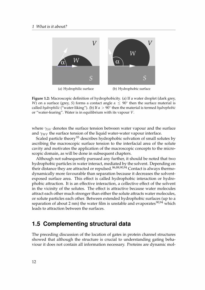
A macroscopic definition of hydrophobicity comes from the observation thata droplet of water W may either completely wet a substrate surface S, form adroplet with a contact angle 0 < α ≤ 90, or a droplet with 90 < α ≤ 180
(Fig. 1.2 on the following page).92 The surface is called hydrophilic in the formertwo cases and hydrophobic in the latter. The contact angle is related to thesurface tension γSW (or free energy to create an interfacial area) by Young’sequation
γSV − γSW − γWV cos α = 0
11
1 What is it about?
Wα
S
V
(a) Hydrophilic surface
W
S
V
α
(b) Hydrophobic surface
Figure 1.2: Macroscopic definition of hydrophobicity. (a) If a water droplet (dark grey,W) on a surface (grey, S) forms a contact angle α ≤ 90 then the surface material iscalled hydrophilic (“water-liking”). (b) If α > 90 then the material is termed hydrophobicor “water-fearing”. Water is in equilibrium with its vapour V.
where γSV denotes the surface tension between water vapour and the surfaceand γWV the surface tension of the liquid water-water vapour interface.
Scaled particle theory93 describes hydrophobic solvation of small solutes byascribing the macroscopic surface tension to the interfacial area of the solutecavity and motivates the application of the macroscopic concepts to the micro-scopic domain, as will be done in subsequent chapters.
Although not subsequently pursued any further, it should be noted that twohydrophobic particles in water interact, mediated by the solvent. Depending ontheir distance they are attracted or repulsed.86,88,90,94 Contact is always thermo-dynamically more favourable than separation because it decreases the solvent-exposed surface area. This effect is called hydrophobic interaction or hydro-phobic attraction. It is an effective interaction, a collective effect of the solventin the vicinity of the solutes. The effect is attractive because water moleculesattract each other much stronger than either the solute attracts water molecules,or solute particles each other. Between extended hydrophobic surfaces (up to aseparation of about 2 nm) the water film is unstable and evaporates90,94 whichleads to attraction between the surfaces.
1.5 Complementing structural data
The preceding discussion of the location of gates in protein channel structuresshowed that although the structure is crucial to understanding gating beha-viour it does not contain all information necessary. Proteins are dynamic mol-
12

1.6 From toy models to the nicotinic receptor
ecules, and a static structure can not quantitate protein movements. Further-more, solvent and solute effects are only addressed insofar as sometimes wateror ions are co-crystallised, thus indicating putative binding sites, or by usingmolecular graphics and displaying the protein surface characteristics, indicat-ing polar and hydrophobic areas. Typically, other methods are also used toprobe different functional aspects and to complement structural data. There isavailable a vast array of biochemical (mutagenesis, fluorescence probe labelling,spin labelling, cysteine scanning mutagenesis, to name a few) and biophysical(patch clamp single channel recordings, flux measurements, . . . ) methods.12
In addition, theoretical and especially computational methods are increasinglyused to model the dynamics of membrane-embedded proteins.95
In this work, computer “simulations” are carried out with the aim to under-stand the behaviour of pure water and of solvated ions in confined geometries,as presented by putative hydrophobic gates in ion channels, i.e. to investigatethe hydrophobic gating hypothesis, and to explore the possibility of such a gatein nAChR. These molecular dynamics calculations treat water, ions, and proteinwith atomistic detail (albeit as a classical not a quantum mechanical system).They allow a dynamic and microscopic view on processes that are difficult orimpossible to observe in experiment. Computer simulations pose a twofoldchallenge: to connect the computational results to experiments, and to under-stand the results in terms of physical models.
The following overview lays out how these aims were approached and met.
1.6 From toy models to the nicotinic receptor
A recurring theme is the question how the behaviour of water and ions de-pends on the environment that is provided by a (protein) pore. In Chapter 2the ground work is laid by recapitulating the thermodynamics and some of thestatistical mechanics of confined fluids. In later chapters this will be used to ex-plain the results of the computer simulations. The bulk of these calculations arefully atomistic molecular dynamics simulations (to be introduced here), both inequilibrium and biased towards unfavourable regions. The latter is performedby umbrella sampling, which is introduced together with the WHAM proced-ure (weighted histogram analysis method) to unbias the biased simulations. Acentral quantity in the discussion of permeation is the potential of mean force(PMF), the free energy required to position a test particle at a given position inspace. The PMF can be obtained from equilibrium and biased simulations. Amore coarse grained approach to the PMF is provided by continuum electro-static Poisson-Boltzmann calculations which allow to calculate the electrostatic(or Born) contribution to the PMF, albeit in a fraction of the computing timerequired for the fully atomistic calculations.
13

1 What is it about?
Chapter 3 introduces a “toy model,” a radically simplified hydrophobic porewith only a limited number of parameters. This provides greater control overthe environment experienced by the permeators and helps to disentangle dif-ferent effects. Although ultimately interested in ion permeation, first the beha-viour of the solvent, i.e. water, is investigated. Despite being little more than ahole through a membrane the toy model system exhibits a wealth of sometimessurprising behaviour. In pores of radius of about 0.5 nm water is seen to oscil-late between a liquid and a vapour phase on a time scale of nano seconds. Nar-row pores of the dimension of the nAChR gate R ≤ 0.35 nm are seen to be voidof water. The absence of liquid water in narrow hydrophobic pores suggeststhat an ion will not be able to permeate the pore because its solvation shell willnot be stable. This chapter is based on O. Beckstein and M. S. P. Sansom, Proc.Natl. Acad. Sci. U.S.A. 100 (2003), 7063–7068 (Ref. 96), but includes extensionsnot presented in the paper and new insights, based on subsequent calculations,which supersede some findings in the original paper.∗
The hydrophobic gating hypothesis is tested in Chapter 4 by extending theprevious calculations to sodium and chloride ions. Equilibrium calculationsdemonstrate that hydrophobic pores of the dimensions of the nAChR gate areimpermeable to ions on the 100 ns time scale. If a narrow hydrophobic poreis made more hydrophilic it can retain liquid water. Thus radius (geometry)and chemical character of the pore wall are identified as determinants of per-meability. A thermodynamic model is developed which explains the liquid-vapour transitions in the pores in terms of surface tensions. So far the chapterclosely follows O. Beckstein and M. S. P. Sansom, Physical Biology 1 (2004), 42–52(Ref. 97). In addition, the effect of pore wall flexibility is investigated and theseemingly counter-intuitive result is found that a flexible pore is less permeableto water than a rigid one. A qualitative argument, which also applies to similarbehaviour at higher temperatures, suggests why this is so.
A quantitative assessment of the impermeability of narrow hydrophobic poresis conducted in Chapter 5 with the calculation of PMFs of ions and water mol-ecules. The barriers to permeation are found to be substantial (> 10 kT) inpores with R < 0.4 nm. This is the strongest evidence in favour of the hydro-phobic gating hypothesis. These atomistic results are compared to continuum-electrostatics calculations which fail to reproduce the molecular dynamics PMFbecause they cannot properly account for the solvent behaviour in the pores.The comparison reinforces the notion that the water in the pore is key to under-standing the behaviour of the ions [O. Beckstein, K. Tai, and M. S. P. Sansom,J. Am. Chem. Soc. 126 (2004), 14694–14695 (Ref. 98)].
After having gained some understanding of the principles of hydrophobic
∗The interested reader will find explained in footnotes where later results improve upon theones published in Ref. 96.
14

1.6 From toy models to the nicotinic receptor
gating from the toy model pores the same reasoning is applied to the poreof the muscle-type nicotinic acetylcholine receptor in Chapter 6. The nAChRstructure only became available in March 2003.29 Historically, the model poreshad been designed to mimic the dimensions of the nAChR pore, based on dataavailable at the time59 (autumn 2000). In 2003 the opportunity arose to com-pare the models to the real structure. Fully atomistic free energy calculationsyield the PMF for Na+, Cl−, and water translocation through the nAChR trans-membrane pore. The permeation barrier is located at the hydrophobic girdle,as predicted by hypothesis. The height and width of the barrier (about 8 kTover 2 nm) strongly supports the idea that the nAChR structure is indeed in theclosed state and that nAChR contains a hydrophobic gate. The results are robustwith respect to different force field parameters and simplifications to the proteinsetup, namely the reduction of the pore to only the five pore lining M2 helices.
The main part closes with a discussion which highlights how the idea of hy-drophobic confinement has already been applied in various systems. Appen-dices list results that could not be incorporated in the main chapters, either be-cause of length or of their more speculative nature. PMFs were calculated for amodel of the neuronal α7 nicotinic receptor41, which show some differences tothe muscle-type nAChR. Other appendices deal with the problem of calculatingvolumes at the molecular scale, which could be used for thermodynamic mod-els such as the one used in Chapter 4, a list of publications which arose from thiswork, and a short overview of software developed for analysis. A bibliographyand an index complete the work.
15


2 Theory and Methods
Before reporting the results on water and electrolytes in a variety of model poresand in the “real” pore of the nicotinic receptor in the next chapters we will setthe scene by recapitulating some of the physics of fluids in inhomogeneous sys-tems, recognising that the theory is the same regardless of the complexity ofthe actual pore. We will then briefly describe the methods used for our ma-chine calculations.∗ Primarily this means atomistic molecular dynamics, bothin equilibrium and as biased simulations, but continuum electrostatics Poisson-Boltzmann theory is also discussed, which is used for Born energy and pKacalculations.
2.1 Thermodynamics and statistical mechanics ofinterfaces
In this work we will be concerned with the behaviour of water or an electrolytein a given environment. In order to interpret the computer simulations somebasic concepts of thermodynamics are required, which are recapitulated in thischapter, following largely Chaikin and Lubensky99, Rowlinson and Widom100,and Hansen and McDonald101.
2.1.1 The surface tension
The environment will take the form of a planar surface (an approximation to abiological membrane) or a pore through such a membrane (a highly simplifiedmodel for ion channels). The difference between a homogeneous bulk system(“water in a box”) and the systems with a membrane-mimetic slab (with orwithout a hole) is the presence of the interface between the slab (the “wall”)and the fluid phase.† The surface introduces a new field, the surface tension or
∗In the early years of computer simulations (1954 to about 1970) theoreticians referred towhat is nowadays known as simulations as machine calculations, as opposed to solving equationswith pencil and paper. Perhaps in the future this particular field will rather be simply knownas computer-assisted biophysics.†The term “fluid” encompasses both the liquid and the gaseous state, which are distin-
guished from the solid state by their higher degree of symmetry. The solid and the liquid(“condensed matter”) differ from the gaseous state in their higher density and degree of spatialcorrelations.99
17
2 Theory and Methods
surface free energy γ, into the total energy U(S, V, N, A),99,100
dU = T dS− p dV + µ dN + γ dA. (2.1)
Here T is the temperature, S the entropy, p the pressure, V the volume, µ thechemical potential of the fluid, N the number of particles in the fluid, and A thearea of the wall-fluid interface. (For an M-component system we would write∑M
i=1 µi dNi =: µ · dN with the chemical potentials of the M species µi and theirparticle numbers Ni.) More useful thermodynamic potentials are the Helmholtzfree energy F(T, V, N, A)
dF = −S dT− p dV + µ dN + γ dA, (2.2)
which is minimal in equilibrium when a closed system∗ is in contact with a heatbath so that the average total energy is fixed, the Gibbs function G(T, p, N, A)(also Gibbs free energy),
dG = −S dT + V dp + µ dN + γ dA (2.3)
(especially useful for biological processes, which typically occur at constantpressure and temperature) and the grand potential
dΩ = −S dT− p dV − N dµ + γ dA. (2.4)
For an open system at equilibrium (which can exchange heat and particles)Ω(T, V, µ, A) takes on a minimal value. The grand potential is best suited for asystem like a pore connected to reservoirs where the chemical potential µ andthe temperature T is fixed by the external reservoir, and the pore volume V isconstant.
Integrating Eq. (2.4) yields
Ω(T, V, µ, A) = −pV + γA, (2.5)
and when this is compared to the grand potential of the homogeneous systemΩ(T, V, µ) = −pV at the same thermodynamic state (T, V, µ) then the excessfree energy
Ωs(T, V, µ, A) := Ω(T, V, µ, A)−Ω(T, V, µ) = γA, (2.6)
is obtained100, i.e. the additional free energy required to create the interface.Hence, the surface tension
γ =Ωs
A=
Ω + pVA
=
(∂Ω∂A
)T,V,µ
(2.7)
∗In a closed system the number of particles is fixed but heat and mechanical energy can beexchanged with the surroundings.
18

2.1 Thermodynamics and statistical mechanics of interfaces
is the free energy required to create the interface per unit of area of the interfacebetween the fluid phase and the wall.∗
2.1.2 Microscopic description
A connection between the microscopic, atomistic parameters (e.g. the inter-action between fluid molecules and the wall) and the macroscopic thermody-namic observables is provided by statistical mechanics. Although we will reallybe concerned with water in the following chapter, by no means a “simple li-quid”, we will restrict the rest of this section to simple liquids made from spher-ical “molecules” because the following equations will not be used in a quantit-ative manner but shall only be used to deepen our understanding of the beha-viour of confined liquids in a very general manner.
The fluid consists of N particles with mass m and momentum pi, which in-teract through a potential V(xj) of the particle coordinates xj alone.† Withoutthe wall, the Hamiltonian H0 is simply
H0(pj, xj) = Hkin +U =N
∑i=1
p2i
2m+ V(xj). (2.8)
Hkin is the kinetic part of the Hamiltonian (here it only contains a translationalcomponent but it can be generalised to non-spherical molecules100). The poten-tial energy U is taken to be an interaction potential V(xj) that only dependson the positions of the N particles.
Canonical ensemble For a given Hamiltonian H the partition function of thecanonical ensemble for N particles is given by
ZN(T, V) = Tr e−βH. (2.9)
β = (kT)−1 is the inverse temperature (with Boltzmann’s constant k =1.3806503(24) × 10−23 J · K−1) and Tr denotes the trace over all states of thequantum mechanical probability density operator or in classical mechanics thephase-space integral
Tr ≡ 1N!
N
∏i=1
∫ d3pi d3xi
h3 .
∗For F a similar relationship, γ = Fs/A, holds, provided the Gibbs dividing surface ischosen as the surface of vanishing adsorption (µ ·Ns = 0).100
†The notation f (xj) ≡ f (xj1≤j≤N) is a shorthand for f (x1, x2, . . . , xN) and indicates thatthe function (or observable) f depends on all coordinates xj. Alternatively this could be writtenf (xN) or f (x3N).
19

2 Theory and Methods
The Helmholtz free energy is then
βF(T, V, N) = − ln ZN(T, V). (2.10)
A thermodynamic average of an observable A(pj, xj) is given by
〈A〉 = Z−1N TrA(pj, xj) e−βH (2.11)
in the canonical ensemble.
Grand canonical ensemble If the number of particles is allowed to vary (butthe average 〈N〉 is fixed by an imposed chemical potential µ) then the partitionfunction of the grand canonical ensemble is
Ξ(T, V, µ) = Tr e−β(H−µN). (2.12)
Now the trace is also summed over all possible numbers of particles 0 ≤ N <∞; classically this means
Tr ≡∞
∑N=0
1N!
N
∏i=1
∫ d3pi d3xi
h3 ;
hence Ξ can also be written Ξ = ∑∞N=0 eβµNZN. The grand potential
βΩ(T, V, µ) = − ln Ξ(T, V, µ) (2.13)
is the thermodynamic potential appropriate for an open system. The thermody-namic average of any observable A is again given as the A-weighted sum overall states, normalised by the partition function
〈A〉 = Ξ−1 TrA(pj, xj) e−β(H−µN), (2.14)
where the grand canonical trace includes the sum over all possible N-states.
Inhomogeneous systems For simplicity, we do not consider the wall a partof the system but represent it through an external field u(x). Then the potentialenergy U must be augmented by the contribution from the external potential
Uext =N
∑i=1
u(xi) =∫
d3x u(x)n(x) (2.15)
20

2.1 Thermodynamics and statistical mechanics of interfaces
with the density(operator)∗
n(x) :=N
∑i=1
δ(x− xi). (2.16)
The inhomogeneous Hamiltonian is thus
H = Hkin +U+Uext = H0 +∫
d3x u(x)n(x). (2.17)
The external potential couples linearly to the density, just as the chemical po-tential [µN =
∫d3x µn(x)]. In the grand canonical ensemble one can interpret
the external potential as a shift in the chemical potential
µ→ µ(x) = µ− u(x), (2.18)
i.e. in the inhomogeneous system the chemical potential appears to depend onthe position.† Hence the grand partition function is now a functional of µ(x),
Ξ[T, V, µ(x)] = Tr e−β(H−µN) = Tr exp[−β
(H0 −
∫d3x µ(x)n(x)
)]. (2.19)
In the homogeneous system the average density 〈n(x)〉 = 〈N〉 /V is constant(where 〈N〉 is fixed through the value of µ). In the system with a wall the addi-tion of the inhomogeneity u(x) will also induce inhomogeneity in the averagedensity,‡ i.e. the variation in µ(x) (or equivalently −u(x)) results in
〈n(x)〉 = δ ln Ξ[µ(x)]δβµ(x)
= −δΩ[µ(x)]δµ(x)
. (2.20)
Not only is the equilibrium density 〈n(x)〉 of interest but also correlations inthe density, which contain information about the local structure of the liquid.
∗The equations from (2.20) onwards are only valid for classical fluids as in the derivationit is assumed that the Hamiltonian H commutes with the local density operator n(x). For thiswork this is no limitation as only classical fluids are simulated by classical molecular dynamicssimulations.†Rowlinson and Widom100 call µ(x) the intrinsic chemical potential µint(x) [their Eq. (4.132)]
and we follow their definition; Chaikin and Lubensky99 prefer to define Uext in (2.15) witha minus sign so that µ(x) = µ + u(x). In either case it is still µ which is fixed in the grandcanonical ensemble.‡The addition of u(x) breaks the symmetry of the homogeneous system H0 so that the in-
homogeneous one has to adapt a lower symmetry; but this route of reasoning will not be furtherpursued in this work.
21
2 Theory and Methods
Scattering experiments effectively measure the two point density correlationfunction99
Cnn(x1, x2) :=
⟨∑i,j
δ(x1 − xi)δ(x2 − xj)
⟩= 〈n(x1)n(x2)〉 . (2.21)
For large separations |x1 − x2| the correlations vanish∗ so that Cnn(x1, x2) tendsto the product 〈n(x1)〉 〈n(x2)〉 (i.e. the densities at the two points are uncorrel-ated). Thus the correlated part of the two point density correlation function isthe Ursell function99
Snn(x1, x2) := Cnn(x1, x2)− 〈n(x1)〉 〈n(x2)〉 . (2.22)
The pair distribution function g(x1, x2), defined by
〈n(x1)〉 g(x1, x2) 〈n(x2)〉 :=
⟨∑i 6=j
δ(x1 − xi)δ(x2 − xj)
⟩= 〈n(x1)n(x2)〉 − 〈n(x1)〉 δ(x1 − x2), (2.23)
is the probability to observe a particle in the volume element d3x at x2, providedthat there is another, different particle at x1. For |x1 − x2| → ∞ it tends to 1; forany liquid whose molecules have a hard core, g(x1, x2) approaches 0 when x2 →x1. For a spatially homogeneous and translationally invariant fluid (〈n(x)〉 =〈n(x + R)〉, hence 〈n(x)〉 = 〈n〉 = 〈N〉 /V), the pair distribution function isonly a function of the difference x = x1 − x2,
g(x) =1〈n〉
⟨∑i 6=0
δ(x− xi + x0)
⟩. (2.24)
For an arbitrary particle at x0, the number of other particles in the volume ele-ment at a distance x equals 〈n〉 g(x) d3x. For isotropic fluids g only depends onthe distance r = |x| from x0 and the number of particles in shells of thickness draround any particle is given by 〈n〉 4πr2g(r) dr ; g(r) is called the radial distri-bution function. For non-isotropic fluids “a” g(r) can still be computed as thespherical average
g(r) = (4π)−1∫ 2π
0dφ
∫ π
0dθ g(r, φ, θ). (2.25)
Occasionally the pair correlation function
h(x1, x2) := g(x1, x2)− 1 (2.26)∗. . . unless the system is close to a phase transition, which is heralded by a diverging correl-
ation length.
22

2.1 Thermodynamics and statistical mechanics of interfaces
is also used, which only contains the correlated part of g(x1, x2). The correlationfunctions can also be obtained as variations δΩ[µ(x)] with δµ(x1) and δµ(x2):
βSnn(x1, x2) = −δ2Ω[µ(x)]
δµ(x1) δµ(x2)=
δ 〈n(x1)〉δµ(x2)
= β(〈n(x1)〉 h(x1, x2) 〈n(x2)〉+ 〈n(x2)〉 δ(x1 − x2)
)(2.27)
Another route to the pair distribution function (2.23) can be taken if the particle-particle interaction potential V(xj) in Eq. (2.8) only consists of pairwise inter-actions v(xi, xj),
V(xj) = ∑i<j
v(xi, xj) =12 ∑
i 6=jv(xi, xj)
=12
∫d3x1 d3x2 v(x1, x2)
[∑i,j
δ(x1 − xi)δ(x2 − xj)−∑i
δ(x1 − x2)δ(x1 − xi)
].
(2.28)
Then it follows immediately that g(x1, x2) is the functional derivative of thegrand potential with respect to the interaction potential,
〈n(x1)〉 g(x1, x2) 〈n(x2)〉 = 2δΩ[v(x1, x2)]
δv(x1, x2). (2.29)
This relationship also explicitly demonstrates that the structure of the liquid (asembodied by g) is rooted in the (pairwise) interaction between fluid particles.The influence of the wall, u(x), is implicitly taken into account by the Boltzmannfactor in the partition function Ξ[u(x)] = Tr exp
[− β
(H0−∑i[µ− u(xi)]
)]. Re-
gions “in” the wall carry a high potential energy for a particle there, whichtranslates into a low probability by virtue of the Boltzmann factor. Hence thisregion of space contributes negligibly to the partition function or any thermo-dynamic average.
Surface tension and density as functionals of the wall potential Becausethe partition functions [Eq. (2.9) or Eq. (2.12)] contain the microscopic paramet-ers in the interaction potential V(xj) and the wall potential u(x) it is possibleto derive expressions for the surface tension which show how it depends onthese parameters. In particular we will be interested in how the surface tensionγ depends on the parameters λj of the wall potential u(x; λj). First we willneed the dependence of the grand potential and the equilibrium density on the
23

2 Theory and Methods
wall parameters,
∂Ω∂λi
=∫
d3x 〈n(x)〉 ∂
∂λiu(x; λj), and (2.30)
∂ 〈n(x1)〉∂λi
= −β∫
d3x2 Snn(x1, x2)∂
∂λiu(x2; λj), (2.31)
which follows from straight differentiation of the partition function (2.12) andEq. (2.13). The surface tension can be obtained as the change of Ω with theinterfacial area A [Eq. (2.7)] and hence
∂γ
∂λi=
(∂2Ω
∂λj ∂A
)T,V,µ
= − 1β
∂
∂λj
∂
∂Aln Ξ[T, V, µ(x), A]. (2.32)
The partial derivative in A is carried out by a dimensional argument.100,101 Forsimplicity, we look at the special case of a flat interface perpendicular to the zdirection. The Cartesian coordinates change by x → (1+ ε)x, y→ (1+ ε)y, andz → (1 + ε)−2z = (1− 2ε)z + O(ε2), where |ε| 1. This distortion conservesthe volume (as required by the partial derivative) and leads to a change in areaδA = 2εA. The only terms affected by the change in coordinates are the onesthat depend on inter-particle distances, i.e. the interaction potential v(xi, xj) in(2.28). The form
γ =12
∫ ∞
−∞dz1
∫d3x12
x212 − 3z2
12r2
12
∂v(r12)
∂r12〈n(x1)〉 g(x1, x2) 〈n(x2)〉
with r12 := |x12| = |x1 − x2| (2.33)
obtained by this approach is called the Kirkwood-Buff formula (where the in-tegration is over all difference vectors x12 := x1− x2). Consequently, the changein the interaction parameters
∂γ
∂λi=
12
∫ ∞
−∞dz1
∫d3x12
x212 − 3z2
12r2
12
∂v(r12)
∂r12
∂
∂λj〈n(x1)〉 g(x1, x2) 〈n(x2)〉 , (2.34)
affects γ only through a change in the pair distribution function
∂
∂λi〈n(x1)〉 g(x1, x2) 〈n(x2)〉 =
− β∫
d3x3
〈n(x1)n(x2)n(x3)〉 − 〈n(x1)n(x2)〉 〈n(x3)〉
+[〈n(x1)n(x2)〉 − 〈n(x1)〉 〈n(x2)〉
]δ(x1 − x2)
∂u(x3; λj)∂λi
(2.35)
24

2.1 Thermodynamics and statistical mechanics of interfaces
Inserting (2.35) into (2.34) shows that the change in surface tension depends on athird order correlation function (the term in curly braces in (2.35)), weighted bythe change of the wall potential ∂u(x; λj)/∂λi. Thus, if u(x) only changes ap-preciably in a narrow region, say, close to the surface, then it will be moleculesin the surface layer that contribute predominantly to the change in surface ten-sion.∗ Eq. (2.34) or (2.33) are not especially useful in their current form becausethe correlation functions and equilibrium densities are not known. One coulduse approximations for 〈n〉 and g (see Rowlinson and Widom100, pp91) but thisis not the subject of this work. These equations are nevertheless useful as aninterpretative guide, which describes where and how changes in the wall influ-ence the equilibrium density and the surface tension, the two quantities that arestudied by computer simulations in subsequent chapters. Furthermore, exactrelations like Eq. (2.34) have been used to accurately calculate surface tensionsfrom the density 〈n(x)〉 obtained from computer simulations.102–104† A moreexhaustive list of sum rules like Eq. (2.34) and (2.31) can be found in van Swoland Henderson102.
2.1.3 Application to computer simulations
In this work, theoretical descriptions as presented in the preceding sections arepredominantly sought to understand and analyse computer simulations. Mo-lecular dynamics simulations (see Section 2.2) yield trajectories of the simulatedsystem, i.e. the position (and if desired, also the velocities) of all particles ateach recorded time step. From a statistical mechanics point of view this is thecomplete though not very enlightening description of the system. Statisticalmechanics and thermodynamic concepts are then applied to extract “interestingproperties.”105 Which observables these correspond to depends on the ques-tions asked and it also depends on the simulation being conducted in such away that the questions can be answered meaningfully.
∗This is rather obvious for a square-well potential102 where the integral in Eq. (2.35) willonly have contributions from within the square well.†Nijmeijer et al.104 obtain a much simpler formula for the change of the surface tension with
the well depth ε of their square well potential, namely
∂γ
∂ε= L−2
∫ L/2
−L/2dx dy
∫ zc
0dz 〈n(x)〉 u(x; ε, a)
ε,
zc being the cut-off for the inter-particle interactions, a the range of the wall potential, and L thesimulation box size. It is not quite clear how they arrived there and how general it is.
25
2 Theory and Methods
Averages
Many equilibrium properties of interest can be expressed as thermodynamicaverages of an observable A, Eq. (2.11) or Eq. (2.14). These averages are ensembleaverages, i.e. the value of the observable for a given configuration A(xi) timesthe probability for this configuration $(xi) = Z−1 exp(−βH) or $(xi) =Ξ−1 exp
(−β(H− µN)
):
〈A〉 = Tr $A (2.36)
From molecular dynamics trajectories one can also compute averages, but theseare time averages of the instantaneous value A(t) := A(xi(t)) of the observableA,
A = limT→∞
1T
T∫0
dt A(t), (2.37)
where T is the time during which the system evolves. The ergodic theoremstates the equivalence of the ensemble average (2.36) and the time average (2.37)in equilibrium.106 In computer simulations, however, finite resources do notallow us to obtain the limit T → ∞.∗ In fact, the ergodic theorem is largelyirrelevant for our purposes because it requires time scales for T which scaleroughly with eN, where N is the number of particles.108 Even for the small sys-tems used in simulations (N = 102 . . . 106) the length of these Poincare cycles isbeyond all computational capabilities.† In practice, the time average Eq. (2.37)can still be a good approximation to Eq. (2.36) for T < ∞, provided that the tra-jectory samples a large enough volume of the relevant phase space110 (where“relevant” is an attribute of configurations xi which contribute strongly tothe average (2.36) due to their large Boltzmann factor).105
Measures of spatial variation A special group of averages measures mobilityor flexibility of particles. A particle in a bound state performs thermal vibrationsabout its equilibrium position x0 = 〈x〉. The range of movement of the particle(or in a certain sense, its flexibility) is characterised by the root mean squaredeviation
ρ :=√〈(x− x0)2〉 =
√(x(t)− x(t))2. (2.38)
As shown in Section 4.3.1 on page 95, ρ can simply be related to a harmonicforce constant, which in turn is a direct measure of how strongly the particle is
∗. . . unless one considers rather non-standard scenarios for the nature of reality, namely a“omega-point” at the end of the universe in a Big Crunch.107
†For N = 100 particles and a time step of ∆t = 1 fs = 10−12 s the simulated time T wouldalready have to be ∆t eN = 2.7× 1031 s = 6× 10¹³ t0 where t0 = 14.1± 0.9× 10⁹ yr is the age ofthe universe.109
26

2.1 Thermodynamics and statistical mechanics of interfaces
bound. An ion or water molecule in solution, on the other hand is not bound butdiffuses freely. In equilibrium, its movement is described by a random walk.111
Thus, the average position of the particle does not change over time (〈x(t)〉 = 0)but the root mean square deviation
ρ(t) :=√〈(x(t)− x(t0))2〉 (2.39)
does. It measures how far on average a particle has drifted. Einstein112 showedthat for a random walk and times t sufficiently larger than the molecular colli-sion time, ρ(t) ∝
√t (see also Eq. (3.12) on page 66 in Section 3.2.3).
Constrained free energies
A general concept in statistical mechanics is the idea of a constrained free en-ergy (for instance, the phenomenological treatment of phase transitions throughLandau free energies).99 We ask what value a free energy W takes on whenan observable A(xi) has a particular prescribed value a. (Depending on thesituation, W could be the Helmholtz free energy F, the Gibbs function G, orthe grand potential Ω.) Calculating the value of W for all a defines the con-strained free energy W(a). The constraint is expressed in the partition functionby performing a partial trace over only those configurations xi where A hasthe value a,
Z(a) := TrA(xi)=a
e−βH and (2.40)
Ξ(a) := TrA(xi)=a
e−β(H−µN). (2.41)
The corresponding constrained free energy is
βF(a) = − ln Z(a) and (2.42)βΩ(a) = − ln Ξ(a). (2.43)
The connection to simulations is established through the probability to observethe system in a state where A takes the value a,
p(A = a) =Z(a)Z
(2.44)
where Z stands for the partition function appropriate for the free energy βW =− lnZ. Z measures the total volume of phase space accessible to the systemwhereas Z(a) describes the (smaller) volume of phase space that is accessibleunder the constraint A(xi) = a. Because all points in phase space have thesame probability weight, the probability to find the system in state a is simply
27
2 Theory and Methods
the quotient of the two phase space volumes. p(a) can be obtained from exper-iments or simulations, and hence the constrained free energy is
βW(a) = − ln p(a) + βW. (2.45)
Because the absolute free energy W is difficult to obtain in most cases, con-strained free energies are often only known up to a constant, i.e. W. It shouldbe noted that W is only a constant with respect to A; if other thermodynamicpotentials like temperature or volume change, then W changes, too. If the ab-solute value of W(a) is required then one possibility is to determine W for areference system analytically and try to bridge between the simulated systemand the reference system. In many cases, however, one is more interested in therelative shape of the energy landscape as a function of a and in these cases theconstant term does not matter.
2.1.4 Volume and other fuzzy concepts
For thermodynamic analysis we would like to be able to compute densities fromthe simulations. It is easy to count particles in a given region of space but in or-der to compute a density one needs to know the volume that is available to theparticle. Often thermodynamics yields surprisingly good results even when ap-plied to microscopic systems though it is by no means required to do so.∗ Anexample is classical nucleation theory which seems to be valid down to clustersof a few atoms.113 When trying to compute a density we are really trying to de-scribe a discrete system (made from particles) by a continuum description (thedensity, defined in the whole of space). In macroscopic and mesoscopic systemsone is used to apply concepts like volume, area, or pressure without furtherthoughts. Rowlinson114 pointed out that these quantities are not well defined atthe molecular scale. A good example is the interface between liquid and vapour.At the length scale of the fluid molecules the interfacial density profile variesover a few molecular diameters.100,101,115 Similarly, the surface between a solidwall, modelled as Lennard-Jones spheres (and not hard spheres), and a fluid iscomplicated because the particles behave like compressible or “squidgy” ballsand not hard billiard balls. Given enough energy, a fluid molecule can approachthe centre of a wall atom arbitrarily close. The problem is hardly a new one, andfor interfaces the concept of the Gibbs dividing surface is well-known,100 wherethe position of the surface is recognised to be arbitrary in the sense that no ther-modynamic function may depend on its position.
Still, it seems desirable to be able to use concepts like “volume”116 or “sur-face area”,117 at least in a consistent fashion (unless one is prepared to com-pletely do without them as suggested by Rowlinson114). Here we describe two∗Equally, there is no obvious reason why it should not give meaningful results for molecular
systems (barring quantum effects).
28
2.1 Thermodynamics and statistical mechanics of interfaces
methods to compute volumes and, more importantly, densities as “number ofparticles divided by some suitable volume”. It should be noted, that the mi-croscopic density n(x) is rather unambiguous when interpreted as the averagenumber of particles in a small volume element d3x as in Eq. (2.16). Problemsarise at boundaries between different phases when macroscopic densities for awhole system are computed from them. For a fluid in the pore the questionreally is what is meant by “in the pore.”
The molecular surface
Qualitatively, a simple van der Waals surface of overlapping “hard sphere”atoms can describe the region of e.g. the pore lumen of an ion channel thatis accessible to solvent. At a higher level of sophistication only the truly solventaccessible surface118 and volume119 are calculated by accounting for re-entrantsurfaces.∗ In a similar manner, the program hole42 traces out the solvent access-ible surface of a pore. All these methods treat atoms as hard spheres with a welldefined radius which is typically taken to be the van der Waals radius. In Ap-pendix B a method to calculate consistent volumes is proposed which explicitlytakes into account the softness of atoms; however, it is not pursued any furtherin the main body of this work.
The basic problem that we face is to calculate the volume of a cylindricalopen pore. The two approaches that are used in the following are simple andtry to define an effective radius that can be used in the same way as hard-spheresurface radius.
Shifted van der Waals surface
Atoms in the pore wall are treated as hard van der Waals spheres, and in fact,they are assumed to form a smooth, unrugged surface, which can be describedby a single radius R. Here R describes the van der Waals surface of the pore, i.e.the interface where the atomic surfaces of a water molecule and a wall atomwould touch.† The neglect of the re-entrant surfaces and of the ruggedness isjustified as calculations of the exact rugged volume (neglecting re-entrancy) ofa pore in Appendix C show.
The effective boundaries between, e.g. fluid and wall, are chosen so that forthe largest system quantities like the density are consistent when calculatedeither from the volume or from an average over small sub volumes. For the
∗The re-entrant surface bounds the regions between overlapping atomic spheres inaccess-ible to the van der Waals surface of a solvent molecule.†The formal definition of the van der Waals surface is the union of the van der Waals spheres
of all atoms in the molecule. Note that this can include internal cavities which are not solventaccessible.
29
2 Theory and Methods
volume of a cylindrical pore this amounts to calculating a correction δR to thevan der Waals surface radius of the interior R by requiring that
π(R + δR)2 L =
L∫0
dz2π∫0
dφ
R0∫0
dr rn(r, φ, z), (2.46)
where R0 is the radius where the density vanishes.∗ (2.46) evaluated for thelargest pore yields the value of δR = −0.03 nm which is used throughout allcalculations. The effective volume from a given pore radius R is hence given
Veff := π(R + δR)2L = πR2effL. (2.47)
(Reff := R + δR is the effective radius.)
Fluid “radius of gyration”
Alternatively, we can estimate the effective radius of a cylindrical cavity by theaverage radius of gyration of the fluid molecules in a disk of thickness dz .† Infact we are interested in R as a function of z, i.e. the pore profile R(z), as it fullycharacterises a cylindrically symmetric pore and can also be used for simpleestimates of the ionic conductance of the pore.12,42 The definition
R2G(z) :=
2∫ 2π
0 dφ∫ R′
0 r dr r2 n(r, φ, z)∫ 2π0 dφ
∫ R′0 r dr n(r, φ, z)
(2.48)
has the correct normalisation so that (2.48) yields the correct result RG(z) =R(z) for a constant, cylindrically symmetric density n(r, z) with a sharp inter-face at R, i.e. n(r, z) = n0(z)Θ
(R(z)− r
), when the integration range R′ ≥ R is
chosen sufficiently large (Θ is the Heaviside step function). RG(z) can be usedas a pore profile; it could be described as an “ensemble pore profile” because it
∗More precisely, R0 should be defined as R0(φ, z) but in practical applications (cf. Sec-tion 3.2.3 on page 62) we computed a radial density first and found R0 as the value where theradial density vanished.†The term “radius of gyration” is used in a rather loose sense for an ensemble of fluid mol-
ecules; it has a much more precise meaning when applied to a single (macro) molecule such asa protein or a simple polymer, which consists of atoms connected by bonds:
RG =
√∑N
i=1 mi (xi − xcom)2
∑Ni=1 mi
,
where xcom is the centre of mass of the polymer consisting of N atoms of mass mi each.
30
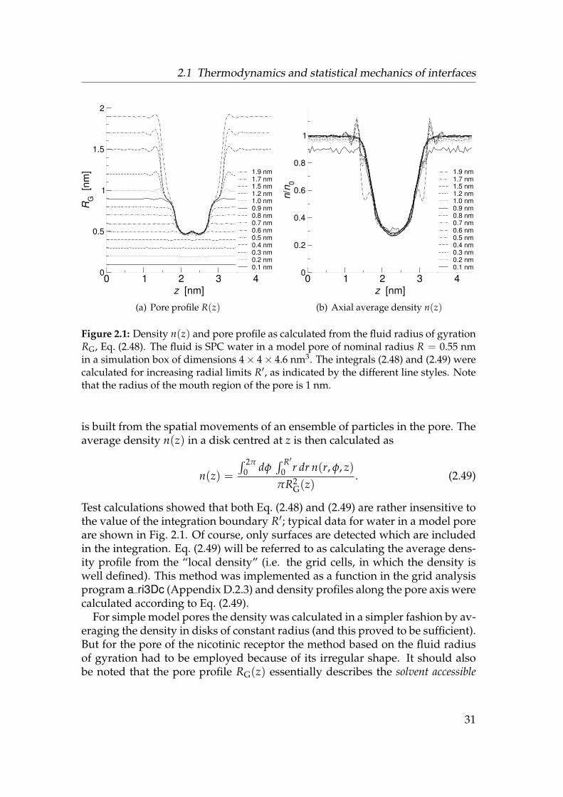
2.1 Thermodynamics and statistical mechanics of interfaces
0 1 2 3 4z [nm]
0
0.5
1
1.5
2
RG [
nm] 1.9 nm
1.7 nm1.5 nm1.2 nm1.0 nm0.9 nm0.8 nm0.7 nm0.6 nm0.5 nm0.4 nm0.3 nm0.2 nm0.1 nm
(a) Pore profile R(z)
0 1 2 3 4z [nm]
0
0.2
0.4
0.6
0.8
1
n/n 0
1.9 nm1.7 nm1.5 nm1.2 nm1.0 nm0.9 nm0.8 nm0.7 nm0.6 nm0.5 nm0.4 nm0.3 nm0.2 nm0.1 nm
(b) Axial average density n(z)
Figure 2.1: Density n(z) and pore profile as calculated from the fluid radius of gyrationRG, Eq. (2.48). The fluid is SPC water in a model pore of nominal radius R = 0.55 nmin a simulation box of dimensions 4× 4× 4.6 nm3. The integrals (2.48) and (2.49) werecalculated for increasing radial limits R′, as indicated by the different line styles. Notethat the radius of the mouth region of the pore is 1 nm.
is built from the spatial movements of an ensemble of particles in the pore. Theaverage density n(z) in a disk centred at z is then calculated as
n(z) =
∫ 2π0 dφ
∫ R′
0 r dr n(r, φ, z)πR2
G(z). (2.49)
Test calculations showed that both Eq. (2.48) and (2.49) are rather insensitive tothe value of the integration boundary R′; typical data for water in a model poreare shown in Fig. 2.1. Of course, only surfaces are detected which are includedin the integration. Eq. (2.49) will be referred to as calculating the average dens-ity profile from the “local density” (i.e. the grid cells, in which the density iswell defined). This method was implemented as a function in the grid analysisprogram a ri3Dc (Appendix D.2.3) and density profiles along the pore axis werecalculated according to Eq. (2.49).
For simple model pores the density was calculated in a simpler fashion by av-eraging the density in disks of constant radius (and this proved to be sufficient).But for the pore of the nicotinic receptor the method based on the fluid radiusof gyration had to be employed because of its irregular shape. It should alsobe noted that the pore profile RG(z) essentially describes the solvent accessible
31

2 Theory and Methods
surface∗ 120 (SAS) of the pore because the calculation is based on the density ordistribution of the centres of mass of the probe particles. Calculating the solventexcluded surface† 122 (SES) is not difficult in principle either. One would have tosmear out the density n(x) with the volume of the probe molecule, modelledby an appropriate shape function χ(r).‡ The new “volumetric” density nV(x)would be the convolution
nV(x) = χ ∗ n =∫
d3x′ χ(x′)n(x− x′).
2.2 Molecular Dynamics Simulations
For comparatively simple systems, analytical methods can already give pro-found insights into the physics of the problem. For more complex systems oneturns to computational methods that integrate the fundamental equations ofmotions of all particles (molecular dynamics) or generate system configurationsaccording to a given thermodynamic ensemble (Monte Carlo methods). Thesemethods are often referred to as “simulations” because they show how a sys-tem behaves which is governed by an approximation to the laws of the realsystem. It does not imply that these simulations or “computer experiments”can be carried out instead of a scientific experiment in the real world. Ideally, acombination of experiment and computer modelling/theory helps us to betterunderstand the problem in question.
2.2.1 The Born-Oppenheimer approximation
A full quantum mechanical description of a molecule is provided by theHamiltonian
H = Te + TN + Vee + VeN + VNN with (2.50)
Te = ∑i
p2i
2m, TN = ∑
N
P2N
2MN,
∗The solvent accessible surface is the surface traced out by the centre of the (spherical) probewhile it rolls over the van der Waals surface of the protein.†The solvent excluded surface is the surface traced out by the probe surface when it rolls
over the van der Waals surface. It may contain re-entrant surfaces which are the concave patches“between” atomic spheres. The interested reader is referred to more specialised articles118,119,121
for a discussion of molecular surfaces.‡Possible shape functions: χ(x) := 1 − exp[−βVrep(|x|)], where the repulsive part of
the Weeks-Chandler-Anderson decomposition123 [Eq. (4.10)] of the Lennard-Jones potential isused; or a Gaussian-like approximation χ(x) := exp[−(|x|/σ)2n], which has the advantage thatthe normalisation 4π
∫ ∞0 dr r2χ(r) can be determined analytically.
32
2.2 Molecular Dynamics Simulations
where H contains the kinetic energy operators for the electrons ‘e’ (mass m)and the nuclei ‘N’ (individual masses MN), the electron-electron interaction, theelectron-nuclei interaction, and the interaction between the nuclei. The positionand momenta of the electrons are denoted xi and pi with x ≡ (x1, . . . xNe), andXN and PN with X ≡ (X1, . . . , XNN).
∗
Born and Oppenheimer124 realised that the large difference in mass betweenelectrons and nuclei leads to an effective separation of the motion of the nucleifrom the electronic motion; the electronic degrees of freedom x adjust instant-aneously to a varying nuclear configuration X.
Following Ref. 125, pp257 we determine the wave function of the electronsψ(x|X) while keeping the nuclear positions X fixed,
(Te + Vee + VeN + VNN)ψ(x|X) = Ee(X)ψ(x|X) (2.51)
where the nuclear positions play the role of parameters in the energy eigenvalue
ε(X) = VNN(X) + Ee(X). (2.52)
ε(X) is the sum of the nuclear interactions and the energy eigenvalue of theelectrons moving in the potential provided by the frozen nuclei. As an ansatzfor the wave function of the whole molecule
Ψ(x, X) = ψ(x|X)Φ(X)
we use a product of the electron wave function at frozen nuclear coordinatestimes the wave function Φ(X) of the nuclei themselves. From the stationarySchrodinger equation HΨ = EΨ follows
ψ(x|X)(TN + ε(X)
)Φ(X) = ψ(x|X) E Φ(X)
−∑N
−h2
2MN
[Φ(X)∇2
X ψ(x|X) + 2∇XΦ(X)∇Xψ(x|X)]
. (2.53)
Multiplying by ψ∗(x|X), integrating over x, and making the Born-Oppenheimerapproximation, i.e. neglecting contributions from the sum over the nuclei(which can be shown to be smaller by a factor m/M ≤ 1/1836 (Ref. 125)), yieldsthe Born-Oppenheimer equation(
TN + ε(X))
Φ(X) = EΦ(X). (2.54)
(2.54) is an effective Schrodinger equation for the nuclei. They move in the ef-fective potential ε(X), Eq. (2.52), and arrange in such a way as to minimise the
∗In this section only we use the notation more common in quantum mechanics, i.e. x forelectrons and X for nuclei. In later sections we will again focus exclusively on the atoms (i.e.essentially the nuclei) and denote their positions with x as was done before.
33

2 Theory and Methods
sum of inter-nuclear Coulomb repulsion VNN and electronic energy Ee, i.e. theequilibrium coordinates of the nuclei are those X which minimise ε(X). Hencethe force on a nucleus K can be calculated as −∇Kε(X1, . . . , XK, . . . , XN), andbecause almost all of an atom’s mass is concentrated in the nucleus, this de-termines the position of the whole atom.
2.2.2 Classical Molecular Dynamics
The Born-Oppenheimer equation Eq. (2.54) implies that the electronic degreesof freedom can be subsumed in an effective potential, and the dynamics of theatoms can be reduced to the classical dynamics of the nuclei in this potential.Then the system of N particles is described by the classical Hamiltonian
H =N
∑i=1
p2i
2mi+ U(x1, . . . , xN), (2.55)
with masses mi, positions xi(t), and momenta pi. U is chosen as to approxim-ate the quantum-mechanical Born-Oppenheimer energy surface Eq. (2.52), i.e.U(x1, . . . , xN) ≈ ε(X). A Newtonian formulation of Eq. (2.55) leads to Newton’sequations of motion126
mi xi = Fi (2.56)
where xi(t) is the acceleration. The force Fi on the i-th particle is derived fromthe potential U,
Fi = −∇iU(x1, . . . , xi, . . . , xN), (2.57)
which depends on the positions of all N particles. A classical molecular dynam-ics trajectory xN(t) :=
(x1(t), . . . , xN(t)
)is generated from integrating Eq. (2.56)
with (2.57) for all particles.The parameterization of U is called a force field and is discussed in the next
section.
2.2.3 Force Fields
A classical force field consists of the functional form of U(xj) (the potentialfunction) and a set of parameters for different atom types. For MD simula-tions the gromacs software package127,128 was used, and so this section fol-lows the package’s implementation notes129 and other standard texts on thesubject.105,130
Potential functions
The potential function U(xj) is a true many body potential which in prin-ciple contains all two-, three- up to N-body interactions. It is approximated
34

2.2 Molecular Dynamics Simulations
by a simpler form containing pairwise-additive two-body potentials for non-bonded interactions and selected two-, three-, and four-body interactions to de-scribe bonded interactions. The classical approximation does not calculate thequantum mechanical wave functions but describes each atom as a mass point,carrying (fractional) point charges, which is bonded to other atoms by harmonic(or other simple) forces—generally referred to as a “balls and springs” model.The functional form of the potential function U is chosen as to give a convenientframe work for parameterization of the Born-Oppenheimer energy surface.
A form typically found in MD force fields is
U = UNB + UB (2.58)
where the first term contains the non-bonded contributions,
UNB(x1, . . . xN) = ∑i<j
VLJ(xi, xj) + ∑i<j
VCoul(xi, xj) (2.59)
(neutral atom interactions and charged atoms interactions). The second oneapproximates bonded interactions with
UB(x1, . . . xN) = ∑(i,j)
Vbond(xi, xj)+ ∑(i,j,k)
Vangle(xi, xj, xk)+ ∑(i,j,k,l)
Vtorsions(xi, xj, xk, xl).
(2.60)
Non-bonded interactions At the quantum mechanical level the only interac-tion that plays a role is the Coulomb interaction between two charged particles.∗
At the classical level the effect of this interaction (in conjunction with the rulesof quantum mechanics) is split up into different separate interactions.
The effect of the Pauli exclusion principle between the valence electrons oftwo atoms at distance r ≡ xij = |xj − xi| is modelled as a steeply repulsivepotential ∝ r−n, n > 6 whereas the dipole-dipole attraction between two neutralatoms is based on a −r−6 term. Taken together, this defines the Lennard-Jonespotential,
VLJ(xij) = 4εij
(σij
xij
)12
−(
σij
xij
)6 , (2.61)
where σij is the distance at which the potential energy vanishes and the energyεij is the depth of the attractive well at the equilibrium separation 21/6σij Analternative equivalent form is
VLJ(xij) =C(12)
ij
x12ij−
C(6)ij
x6ij
. (2.62)
∗Gravitation is much weaker than the electrostatic force and neither strong nor weak forcehave a direct influence on the behaviour of atoms due to their short range.
35
2 Theory and Methods
The parameters C(12)ij and C(6)
ij (or εij and σij) depend on the atom types of thepair (i, j).∗ If a particular combination has not been explicitly parameterized thecross terms can be calculated by the empirical combination rules
C(6)ij =
√C(6)
ii C(6)jj and C(12)
ij =
√C(12)
ii C(12)jj (2.63)
or
σij =12(σii + σjj) and εij =
√εii εjj. (2.64)
Electrostatic (Coulomb) interactions are calculated from Coulomb’s lawbetween two charged particles as
VCoul(xij) =1
4πε0
qiqj
xij. (2.65)
An important step in the parameterization of a force field is the assignment ofpartial charges qi to atoms of a molecule; these partial charges interact throughEq. (2.65).
Bonded interactions Two atoms connected by a chemical bond behave likea classical harmonic oscillator for small deviations from their equilibrium bondlength. Hence bonds are typically represented by a harmonic bond-stretchingpotential
Vbonds(xij) =kb
ij
2(xij − bij
)2 (2.66)
around the atom-type dependent equilibrium bond length bij with a force con-stant kb
ij. An equally valid approximation is a fourth-power potential†
Vbonds(xij) =kb
ij
4
(x2
ij − b2ij
)2. (2.67)
Directionality of bonds is incorporated through angle potentials which embodyharmonic angular vibrations between three atoms (i, j, k),
Vangle(θijk) =kθ
ijk
2(θijk − αijk
)2 with θijk := arccosxji · xjk
xjixjk, (2.68)
∗The relation between the two parameter sets is σ = (C(12)/C(6))1/6 and ε =14 (C
(6))2/C(12), or C(6) = 4εσ6 and C(12) = 4εσ12.†The force constants in Eq. (2.66) and (2.67) are related by 2 kb
ij bij = kbij.
36

2.2 Molecular Dynamics Simulations
where αijk is the equilibrium angle between atoms of the types represented byi, j, and k.∗ Sometimes a simplified version of Eq. (2.68) is used instead,†
Vangle(θijk) =kθ
ijk
2(cos θijk − cos αijk
)2 with cos θijk :=xji · xjk
xjixjk. (2.69)
Torsional vibrations are described by dihedral potentials. The dihedral anglebetween the planes (i, j, k) and (j, k, l) is defined by
φijkl = arccos(xji × xjk) · (xkl × xjk)
|xji × xjk| · |xkl × xjk|(2.70)
so that φijkl = 0 when i and l are in the cis conformation (the IUPAC/IUB con-vention). One choice for a periodic dihedral potential is
Vdih(φijkl) = kφijkl
(1 + cos(nφijkl − φ0,ijkl)
)(2.71)
with dihedral force constant kφijkl (typically depends only on atom types of j
and k), multiplicity n and phase shift φ0,ijkl. Another choice is the Ryckaert-Bellemans form
Vdih(φijkl) =5
∑n=0
Cn cosn(φijkl − π). (2.72)
A special form of (2.72) is used in the OPLS-AA force field,
Vdih(φijkl) = V0 +12
3
∑n=1
Vn(1 + cos nφijkl), (2.73)
which are the first four terms of a Fourier series in the dihedral potential. Animproper dihedral angle ξijkl is defined in the same way as φijkl in Eq. (2.70) butthe four atoms can also be part of a tetrahedral or a ring structure. The improperdihedral potential
Vimpr(ξijkl) = kξijkl(ξijkl − ξ0,ijkl)
2 (2.74)
is used to keep rings planar or prevent molecules from flipping over to theirmirror image.
In the following sections the values that were chosen for the parameters inEqs. (2.61) to (2.74) are briefly discussed.
∗The definition used for connecting vectors i→ j is xij := xj − xi.†The force constants in Eq. (2.68) and (2.69) are related by kθ
ijk sin2 αijk = kθijk.
37
2 Theory and Methods
Protein force field
For a simulation, parameters have to be chosen for the protein, ligands, water,and ions. All these parameter sets have to be compatible and some care needsto be taken when combining different parameter sets.
Model pores Many simulations in this work were carried out on systems con-taining primarily water and model pores, which are much simpler than real pro-teins. These pores were constructed from methane molecules (see in particularSection 3.2.1 and also Appendix D.1.1) to make them hydrophobic. A methanemolecule is modelled as a unified atom, i.e. the effect of the hydrogen atoms isincorporated into the LJ potential of the unified CH4 “atom”. The LJ paramet-ers for the interaction between a methane molecule and the water oxygen areεCO = 0.906493 kJ mol−1 and σCO = 0.342692 nm and were taken directly fromthe GROMOS96 force field.
Proteins Today there exists a range of well-tested force fields suitable for mo-lecular simulations of proteins.131 In Chapter 6 calculations are carried out fortwo different force fields to assess the reliability of the results.
The GROMOS96132,133 force field is a united atom force field, i.e. it treatsnon-polar hydrogen atoms as part of a larger united atom; hydrogens on aro-matic rings and polar hydrogens are treated explicitly.∗ The united atom schemereduces the typical system size from about 15 000 atoms to about 10 000 (cf.Tab. 6.1 on page 132) with a corresponding speed up in simulation execution.GROMOS96 uses Eq. (2.67) for bonds, Eq. (2.69) for angles, Eq. (2.71) for properdihedrals, and all other interactions as described in Section 2.2.3.
The second force field, OPLS-AA 134–140, is an all atom force field, which treatsall hydrogens explicitly.† An all atom force field is arguably a better choicewhen it comes to investigating hydrophobic gating. The important hydro-phobic side chains are modelled as unified atoms in GROMOS96 but simula-tions of model pores showed that the wall-water interaction is important andconceivably a better description of this interaction is provided if all hydrogenatoms are present as is the case in OPLS-AA. The functional form of OPLS-AAdiffers from GROMOS96 in that bonds are calculated by Eq. (2.66), angles byEq. (2.68), and proper dihedrals by Eq. (2.72).
GROMOS96 is optimised with the SPC water model132 whereas TIP4P141 isthe native water model of OPLS-AA. For long (50 ns) simulations of the 36-residue Villin headpiece van der Spoel and Lindahl142 evaluated combinations∗All hydrogens were “dummified”, i.e. their position was calculated from the position of
their connecting heavy atoms,129 saving the calculation of forces and speeding up the calcula-tion.†Hydrogens were dummified129 as for GROMOS96.
38
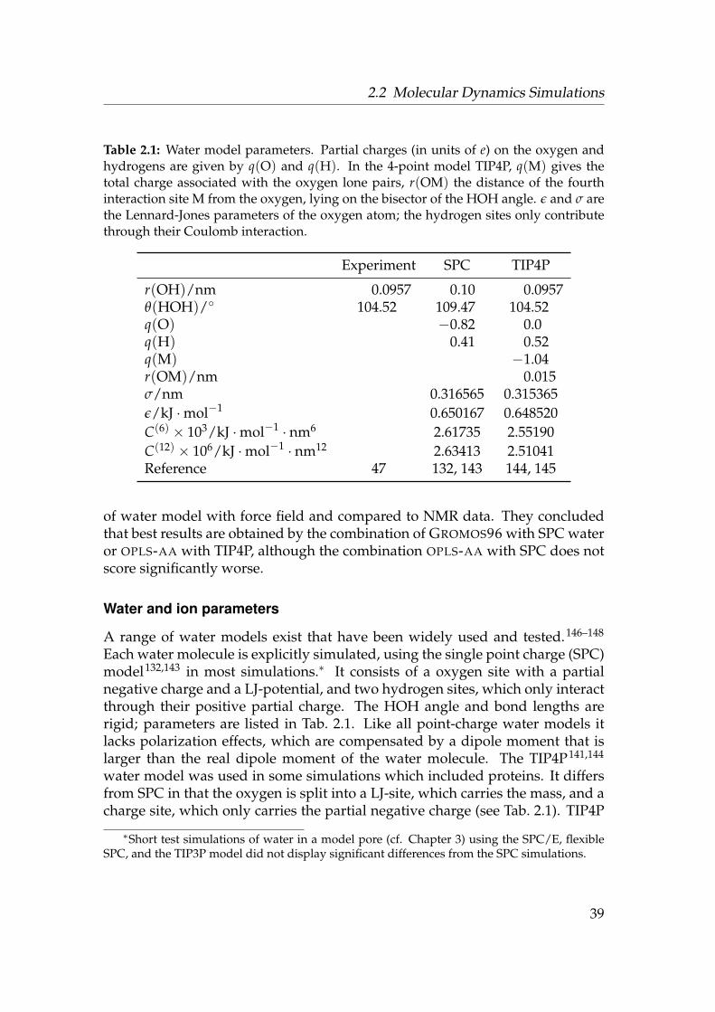
2.2 Molecular Dynamics Simulations
Table 2.1: Water model parameters. Partial charges (in units of e) on the oxygen andhydrogens are given by q(O) and q(H). In the 4-point model TIP4P, q(M) gives thetotal charge associated with the oxygen lone pairs, r(OM) the distance of the fourthinteraction site M from the oxygen, lying on the bisector of the HOH angle. ε and σ arethe Lennard-Jones parameters of the oxygen atom; the hydrogen sites only contributethrough their Coulomb interaction.
Experiment SPC TIP4P
r(OH)/nm 0.0957 0.10 0.0957θ(HOH)/ 104.52 109.47 104.52q(O) −0.82 0.0q(H) 0.41 0.52q(M) −1.04r(OM)/nm 0.015σ/nm 0.316565 0.315365ε/kJ ·mol−1 0.650167 0.648520C(6) × 103/kJ ·mol−1 · nm6 2.61735 2.55190C(12) × 106/kJ ·mol−1 · nm12 2.63413 2.51041Reference 47 132, 143 144, 145
of water model with force field and compared to NMR data. They concludedthat best results are obtained by the combination of GROMOS96 with SPC wateror OPLS-AA with TIP4P, although the combination OPLS-AA with SPC does notscore significantly worse.
Water and ion parameters
A range of water models exist that have been widely used and tested.146–148
Each water molecule is explicitly simulated, using the single point charge (SPC)model132,143 in most simulations.∗ It consists of a oxygen site with a partialnegative charge and a LJ-potential, and two hydrogen sites, which only interactthrough their positive partial charge. The HOH angle and bond lengths arerigid; parameters are listed in Tab. 2.1. Like all point-charge water models itlacks polarization effects, which are compensated by a dipole moment that islarger than the real dipole moment of the water molecule. The TIP4P141,144
water model was used in some simulations which included proteins. It differsfrom SPC in that the oxygen is split into a LJ-site, which carries the mass, and acharge site, which only carries the partial negative charge (see Tab. 2.1). TIP4P
∗Short test simulations of water in a model pore (cf. Chapter 3) using the SPC/E, flexibleSPC, and the TIP3P model did not display significant differences from the SPC simulations.
39
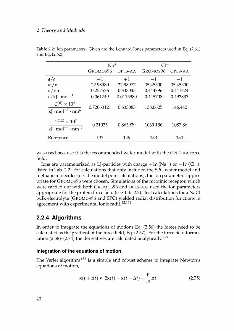
2 Theory and Methods
Table 2.2: Ion parameters. Given are the Lennard-Jones parameters used in Eq. (2.61)and Eq. (2.62).
Na+ Cl−
GROMOS96 OPLS-AA GROMOS96 OPLS-AA
q/e +1 +1 −1 −1m/u 22.98980 22.98977 35.45300 35.45300σ/nm 0.257536 0.333045 0.444796 0.441724ε/kJ ·mol−1 0.061749 0.0115980 0.445708 0.492833
C(6) × 104
kJ ·mol−1 · nm60.72063121 0.633083 138.0625 146.442
C(12) × 107
kJ ·mol−1 · nm120.21025 0.863929 1069.156 1087.86
Reference 133 149 133 150
was used because it is the recommended water model with the OPLS-AA forcefield.
Ions are parameterized as LJ-particles with charge +1e (Na+) or −1e (Cl−),listed in Tab. 2.2. For calculations that only included the SPC water model andmethane molecules (i.e. the model pore calculations), the ion parameters appro-priate for GROMOS96 were chosen. Simulations of the nicotinic receptor, whichwere carried out with both GROMOS96 and OPLS-AA, used the ion parametersappropriate for the protein force field (see Tab. 2.2). Test calculations for a NaClbulk electrolyte (GROMOS96 and SPC) yielded radial distribution functions inagreement with experimental ionic radii.12,151
2.2.4 Algorithms
In order to integrate the equations of motions Eq. (2.56) the forces need to becalculated as the gradient of the force field, Eq. (2.57). For the force field formu-lation (2.58)–(2.74) the derivatives are calculated analytically.129
Integration of the equations of motion
The Verlet algorithm152 is a simple and robust scheme to integrate Newton’sequations of motion,
x(t + ∆t) ≈ 2x(t)− x(t− ∆t) +Fm
∆t. (2.75)
40

2.2 Molecular Dynamics Simulations
It can be derived from the Taylor expansion of x(t + ∆t) + x(t − ∆t).105,130,153
The error in the positions is of order ∆t4; velocities v(t) = 12∆t(x(t + ∆t)− x(t−
∆t))+ O(∆t2) are less accurate but are only required to compute the kinetic
energy and thus the temperature. The Verlet algorithm has good long time sta-bility and energy conservation because it is a symplectic integrator. It is not justa scheme to solve a set of differential equations but it also conserves propertiesinherent in a Hamiltonian system, namely energy conservation, time reversalsymmetry, volume of phase flow and the sum of areas of phase elements.130,153
Leap-frog integrator In gromacs a variant of the Verlet integrator is em-ployed, the leap-frog algorithm,154 which defines the velocities at half-integertime steps105,129,130,153
v(t + 12 ∆t) :=
x(t + ∆t)− x(t)∆t
and v(t− 12 ∆t) :=
x(t)− x(t− ∆t)∆t
.
This leads to the update for the positions
x(t + ∆t) ≈ x(t) + v(t + 12 ∆t)∆t (2.76)
and the update of the velocities is taken from the Verlet scheme (2.75)
v(t + 12 ∆t) ≈ v(t− 1
2 ∆t) +Fm
∆t. (2.77)
It can be shown to be formally equivalent to the Verlet scheme and thus sharesits symplectic properties, but has the advantages of a smaller error on the velo-cities and is less prone to the introduction of numerical imprecision.105
Bond constraining The time step ∆t in the integration scheme depends onthe fastest motions in the system. For liquids and biomolecules in the biologicaltemperature range these are bond vibrations, which are about 10–50 times fasterthan translational motions.153 By treating harmonic bonds as rigid, time stepscan be increased by about a factor of four.155 Rigid bonds are implemented asconstraints, which are enforced after each time step by resetting the bonds totheir fixed length. For protein bonds the LINCS155 algorithm was employed(an improvement over traditional SHAKE156 in terms of stability and speed),whereas for the rigid water models the optimised SETTLE157 procedure wasused.
Electrostatics under periodic boundary conditions
The size of the systems that can be currently simulated with MD is still so smallthat the surface region of the system is large compared to the volume. Because
41

2 Theory and Methods
one is interested in volume behaviour the surface is eliminated by periodic-ally repeating the simulation cell, known as periodic boundary conditions. Aparticle exiting on one side of the cell enters from the opposite face with thesame velocity.
Care must be taken when calculating non-bonded interactions. For shortrange interactions, which decay faster than r−3 a simple cut-off scheme suffices,where these interactions are only calculated between particles i and j within acut-off radius Rcut when |xij| ≤ Rcut. The cut-off radius cannot be larger thanthe shortest cell dimension.
The Coulomb interaction (2.65), however, has a long range and in a periodic,i.e. crystal-like, arrangement contributions from an infinite number of neigh-bouring image cells need to be considered.158 Truncation (cut-off) schemes existfor long range forces with varying degrees of sophistication. In particular forwater and electrolytes they have been shown to introduce serious artifacts dueto ordering just outside the cut-off region.158,159 In this work great emphasis isput on the behaviour of water and ions and hence an exact method was chosento evaluate all contributions to the Coulomb energy. It is based on the Ewaldsummation method,160 initially devised to calculate the electrostatic energy ofionic crystals.
Following Deserno and Holm161 the total electrostatic energy of a periodicsystem (box length L, periodic in three dimensions n = (n1, n2, n3)) can be writ-ten as
UCoul =1
4πε0
12
N
∑i,j=1
∑′
n∈Z3
qiqj
|xij + nL| , (2.78)
where the primed sum indicates that for i = j the term n = 0 has to be omitted.Eq. (2.78) is only conditionally convergent so its value actually depends on thelimiting procedure employed.158 The slowly converging sum can be split intotwo fast converging ones, based on the identity
1r=
f (r)r
+1− f (r)
r;
one term collects the rapid variations for short distances, the other theslow decay at large separations. The Ewald choice f (r) = erfc(r) :=
2√π
∫ +∞r dt exp(−t2) screens the point charges by Gaussian charge densities
(which makes their interactions decay rapidly with distance) and then correctsfor the lattice of screening charges (which can be computed in reciprocal space).The Ewald energy is
UCoul = U(r) + U(k) + U(s) + U(d), (2.79)
42

2.2 Molecular Dynamics Simulations
where the contribution from real space is (now using Gaussian units for nota-tional convenience)
U(r) =12 ∑
i,j∑′
m∈Z3
qiqjerfc(α|xij + mL|)|xij + mL| , (2.80)
from reciprocal space
U(k) =1
2L3 ∑k 6=0
4π
k2 e−k2
4α2 |ρ(k)|2, (2.81)
the self-energy
U(s) = − α√π
∑i
q2i , (2.82)
and the dipole correction
U(d) =2π
(1 + 2ε′)L3
(∑
iqixi
)2
. (2.83)
The Fourier transform of the charge density ρ(x) is
ρ(k) =∫
d3x ρ(x)e−ik·x =N
∑j=1
qje−ik·xj . (2.84)
The Ewald tuning parameter α adjusts the relative contributions of real andreciprocal space terms. The advantage of splitting Eq. (2.78) in such a way isthat the sums (2.80) and (2.81) converge exponentially with m and k and so asmall cut-off can be chosen for them without much loss of accuracy.153,158,161
CPU time for the Ewald summation scales with N3/2 due to the Fourier sumEq. (2.81) with (2.84), which is O(N2).153 For large systems a more efficientapproach to computing U(k) is provided by the Fast Fourier Transform (FFT,Ref. 162), which is O(N log N). However, FFT requires the charges to be loc-ated on a regular grid or mesh. Deserno and Holm161 present a careful studyof a number of algorithms (particle-particle/particle-mesh (PPPM, Ref. 163),particle-mesh (PME, Ref. 164), and smooth PME (SPME, Ref. 165) Ewald sum-mation; the SPME method was used in this work), which all employ the sameidea: First the particle charges are spread or interpolated over a regular mesh.Then the mesh density is fast-Fourier transformed (the equivalent of Eq. (2.84))and the reciprocal space energy U(k) (analogously to Eq. (2.81)) is evaluated
43

2 Theory and Methods
(this amounts to solving Poisson’s equation). Then forces on the interpolatedcharges are calculated as the derivative of the Coulomb energy (SPME calcu-lates analytical derivatives, which is fast in terms of computational speed butnot as exact as a Fourier space derivative, i.e. multiplication by ik, Ref. 161). Fi-nally, the forces are back-interpolated on the original particle positions to yieldthe Coulomb contribution to the total force on the particle.
All calculations in the following chapters employed the SPME165 method andused the same set of parameters: the real space cutoff in Eq. (2.80) was 1 nm,the Fourier spacing was 0.15 nm−1 (which fixes the maximum wave vector inthe sum Eq. (2.81)), and α = 10−5. Fourth order cubic splines were used inthe SPME interpolation procedure. These parameters should give electrostaticenergies accurate to 5× 10⁻³, which is better than the typical accuracy of the LJterms.129
Constant temperature, constant pressure simulations
Laboratory experiments are typically conducted under conditions of constanttemperature and constant pressure. The trajectories obtained from the Hamilto-nian (2.55) are total energy conserving and thus the system is described by themicrocanonical ensemble. Different schemes have been proposed to generateother ensembles. The first class of schemes modifies Eq. (2.55) and are knownas extended Hamiltonian methods;130,153 they can be shown to generate welldefined thermodynamic ensembles. Methods of a second class, named weakcoupling schemes,130,166 are conceptually simpler but do not lead to an exactlydefined ensemble, although the practical deviations are believed to be negli-gible.129 In this work, the weak coupling schemes were used to simulate at con-stant temperature and pressure.
Temperature coupling The temperature T is computed from the velocitiesthrough the kinetic energy of the whole system,
12 ν kT = Ekin = 1
2
N
∑i=1
miv2i with ν := 3N − Nconstraints − νcom, (2.85)
where ν is the number of degrees of freedom, i.e. all translational degrees ofspherical atoms minus the number of constraints applied to these atoms (e.g.fixed bond lengths) and νcom = 3 for centre of mass momentum removal. Ifone of the constant temperature algorithms is employed then the centre of massmomentum must be periodically removed from the simulation to avoid a trans-fer of energy to the centre of mass, which leads to a cooling of the atoms whilethe total system accelerates—an effect known as the “flying ice cube”;167 this is
44
2.2 Molecular Dynamics Simulations
not a problem for constant energy simulations as the Verlet algorithm has verygood momentum conservation properties.
As described in Ref. 129, the weak coupling algorithm166 mimics the couplingto a heat bath with a given temperature T0. The effect is a slow relaxation of thesystem temperature T to the target temperature T0 according to
dTdt
=T0 − T
τ.
Initial deviations will exponentially decay with constant τ. The algorithmchanges the particle velocities at each step by a factor λ, which is calculatedas
λ =
√√√√1 +∆tτT
(T0
T(t− 12 ∆t)
− 1
)where τ = τT
2CV
kν, (2.86)
CV being the system’s heat capacity at constant volume. The use of the leap-frog algorithm Eq. (2.77) limits the temperature to the one at the last half-step.In gromacs τT and T0 can be prescribed. τ/τ0 varies between 1 (ideal gas CV =32 Nk) and about 3 for water. In all simulations reported here, a long decay timeof τT = 0.1 ps was chosen as to only minimally influence the dynamics of thesystem (for a step size ∆t = 2 fs = 2× 10⁻³ ps).
Pressure coupling The instantaneous pressure p(t) is computed as the trace
p = 13 Tr p (2.87)
of the pressure tensor
p =2V
(12
N
∑i=1
mivi ⊗ vi − Ξ
)(2.88)
from the virial tensor
Ξ =12 ∑
i<jxij ⊗ Fij. (2.89)
Simulations at constant pressure were also carried out with the help of a weakcoupling scheme,166 which rescales the particle coordinates xi and simulationcell vectors at each time step with a scaling matrix
µij = δij −∆t3τp
βij(
p0,ij − pij(t))
. (2.90)
45

2 Theory and Methods
τp is the coupling time constant and β is an estimate for the isothermal com-pressibility of the system; it suffices to choose a value applicable to liquids likethe one for water, β = 4.6× 10⁻⁵ bar−1. This scheme also leads to a exponen-tially damped relaxation
dp
dt=
p0 − p
τp.
All simulations were carried out at p0 = 1 bar with a slow relaxation time ofτp = 1 ps. Pressure coupling was only applied in the z-direction, parallel tothe pore axis by setting all βij = 0 except for βzz = 4.5× 10⁻⁵ bar−1. This keptthe “membrane” in the xy-plane of the simulation cell at constant size while thesimulation cell could adjust in the direction perpendicular to the membrane.∗
2.3 Free energy calculations
Free energies such as the Helmholtz free energy, the Gibbs function, or thegrand potential are important quantities in the description of thermodynamicsystems in equilibrium because—depending on the boundary conditions—oneof them takes on a minimum value in equilibrium. A system displaced fromequilibrium by a change of constraints will rearrange in such a way that its freeenergy becomes minimal again while satisfying the constraints. By comparingthe constrained free energy W(A = a) (introduced in Section 2.1.3) for differ-ent values a and a′ of the constraint A one obtains the reversible work requiredfor the transition from state a to state a′. For instance, a could be the state “aparticular Na+ ion is in the bulk” and a′ “the ion is in the channel pore.” IfW(a′) > W(a) then the presence of ion in the pore would be disfavoured bythe Boltzmann factor exp[−β
(W(a′)−W(a)
)], and the system is more likely to
be found with no ions in the pore. The free energy is grounded in a statisticalmechanics description of the system and contains both enthalpic and entropiceffects, unlike simple calculations of interaction energies.
2.3.1 The potential of mean force
A particularly useful constrained free energy is obtained when the constraint istaken to be the position x1 of a tagged particle 1 such as a water molecule oran ion. The resulting potential of mean force168 (PMF) W(x1) is the free energyrequired to position the particle at the position x1, relative to some reference
∗The “membrane” was actually mimicked by an Einstein crystal of hydrophobic methanemolecules (see Section 3.2.1 on page 60 for details), which lent itself naturally to a simulation atfixed area.
46

2.3 Free energy calculations
state. The PMF itself is the most fundamental quantity for the description ofpermeation and can be used as an input to more coarse grained methods tocompute I-V curves or single channel conductances from first principles.169 ThePMF can be written as169
e−βW(x1) = C∫
d3x2 · · · d3xN e−βU(x1,x2,...,xN), (2.91)
where all coordinates are integrated out except for the coordinate of the particleof interest; C is a constant fixed by the reference state. The name “potential ofmean force” derives from the fact that the gradient −∇1W(x1) is the effectiveor mean force that is exerted on particle 1 by all other particles 2 to N in thesystem.∗
For transport processes it is convenient to define a reaction coordinate ξwhich parameterizes the path x(ξ) that a particle of interest moves along. Thenthe PMF along ξ becomes a one dimensional (1D) free energy profile
e−β[W(ξ)−W(ξ0)] = C
∫d3x1 · · · d3xN δ
(x(ξ)− x1
)e−βU(x1,x2,...,xN)∫
d3x1 · · · d3xN δ(x(ξ0)− x1
)e−βU(x1,x2,...,xN)
, (2.92)
where ξ0 is a reference point, and C is again arbitrary. In the case of straight ionchannels and pores with their pore axis parallel to the z-axis, ξ is generally takento be the z coordinate of the particle.12 Such a 1D free energy profile is used asan input to simple kinetic rate theory and 1D Nernst-Planck models.12,95,169 Thereduction of the dimensionality of the PMF is only justified if z is a good reactioncoordinate, i.e. all other degrees of freedom reach equilibrium rapidly whilst zis only slowly varying;95,169 in this case the PMF can be written as
e−βW(z) := e−β[W(0,0,z0)−µ0]
∫dx∫
dy e−βW(x,y,z)∫dx∫
dy e−βW(x,y,z0)(2.93)
where the normalisation was chosen so that the PMF vanishes in the bulk farfrom the pore (µ0 being the excess chemical potential of the sampled species inthe bulk). Eq. (2.93) shows that W(z) is only meaningfully defined in the poreregion where the integration over x and y is bounded. Far from the channel, the1D PMF is ill defined.169,170 The 3D PMF W(x) ≡ W(x1) (2.91) does not sufferfrom this shortcoming and can be used to relate the 1D PMF in the pore to theconstrained free energy in the bulk. The constant C in Eq. (2.92) is arbitrary,and hence there is no unique definition of W(z) (which allows the choice madein (2.93)) and only the variations within the PMF along z are meaningful; the3D PMF is required to make statements about all processes which involve a
∗Ref. 169 defines the PMF in a more rigorous and general way but for the present purposethe definition of the one-particle PMF W(x) should suffice.
47

2 Theory and Methods
particle in the bulk and in the channel, e.g. binding energies in the pore orbarrier heights.
The PMF is related to the equilibrium density∗ n(x) through the density ofthe reference state in the bulk far from the pore n0,
βW(x) = − lnn(x)n0
+ β(W0 − µ0), (2.94)
because n(x)/n0 d3x is the probability to find the particle at position x. Simil-arly, the 1D PMF is
βW(z) = − lnn(z)n0
+ β(W0 − µ0) with (2.95)
n(z) =1A
∫dx∫
dy n(x), (2.96)
where A is the area in the xy-plane which is integrated over.
2.3.2 Umbrella sampling
From equilibrium MD trajectories the density n(x) can be determined, and withthe help of Eq. (2.94) also the PMF (up to the constant term). However, in mostcircumstances it is not possible to reliably estimate the density from simula-tions because a region of large PMF corresponds to a region of low occupancy.Furthermore, particles might be unable to cross a barrier (a local maximum inW(ξ)) to explore regions of space behind the barrier.† The umbrella samplingmethod of Valleau and Torrie172 (see also Ref. 173) overcomes the problem ofinsufficient sampling for certain regions on the reaction coordinate ξ by intro-ducing an additional biasing potential w(ξ) which forces the sampled particleinto the high energy regions.‡ The biased simulations are generated using the
∗From here onwards the symbol n(x) should be understood as the expectation value of thedensity operator Eq. (2.16), i.e. as 〈n(x)〉.†Example to illustrate the difficulty to sample a barrier region in equilibrium MD (following
Smith and Sansom171): The rate of barrier crossing k is assumed to follow an Arrhenius law
k = v exp(−βG‡).
The activation energy G‡ is taken as the barrier height, for instance G‡ = 40 kT (see Chapter 5for an example). With an estimate of the jump attempt frequency of a Na+ ion across the barrieras v = 1 ps−1, we arrive at a mean time between successful jumps of τ ≈ 2.4× 10⁵ s = 65 h.A typical MD simulation of the system runs at 1 ns simulated time per 10 h real wall-clocktime. To observe a single successful barrier crossing one would need to simulate on average for2.4× 1014 h = 27 Gyr = 1.9 t0 where t0 = 14.1± 0.9× 10⁹ yr is the age of the universe.109
‡The further discussion will generally follow Roux174, which is more accessible than theoriginal publication.172
48

2.3 Free energy calculations
-0.05 0.05 0.1 0.15z
0.5
1
1.5
2
WHzLk T
(a) Step potential
-0.1 -0.05 0.05 0.1 0.15 0.2 0.25z
10
20
30
40
PHz, z0 L
(b) Probability densities
Figure 2.2: Probability density for a harmonically restrained particle at a step barrier.(a) The PMF has the shape of a step function of height 2 kT, centred on z = 0.05,βW(z) = 2Θ(z− 0.05). (b) A test particle in this PMF is restrained to a window centrez0 with a harmonic force. The probability of the particle to be in an interval [z, z + dz]can be calculated analytically (see Appendix D.3.2) and plotted for different z0. Theprobability distribution at the discontinuity z0 = 0.05 is highlighted.
new potential energy U(xj) + w(ξ). Typically, a number of simulations withdifferent biasing potentials are carried out, each one confining the variations inthe position of the particle to a particular region or “window” i on ξ (whencethe method derived the name umbrella sampling). A common choice for thewindow potentials wi is a harmonic one,
wi(ξ) =12 K (ξ − ξi)
2, (2.97)
which restrains the particle to the vicinity of the window centre ξi. The wi arechosen so to overlap and cover the whole range of interest on the reaction co-ordinate. In practice, an equilibrium simulation is run for each window i andthe probability distribution of ξ is recorded during the run. The results from allwindows are unbiased and combined to yield the PMF.
An example for the influence of umbrella windows on the distribution of atest particle is shown in Fig. 2.2. The PMF is a step barrier and in the regionsof constant PMF the probability distribution is Gaussian, as expected for a har-monically bound particle. Close to the barrier, the Gaussian distribution is dis-torted by the influence of the PMF, and it is this difference from the knownGaussian distribution which allows the calculation of the underlying PMF.
49
2 Theory and Methods
The average distribution function (or density) is
〈ρ(ξ)〉 :=
∫d3x1 · · · d3xN δ
(ξ(xj)− ξ
)e−βU(xj)∫
d3x1 · · · d3xN e−βU(xj), (2.98)
where the reaction coordinate typically only depends on a subset of all xi. Interms of the average distribution function, the PMF is (cf. Eq. (2.95))
W(ξ) = −β−1 ln〈ρ(ξ)〉〈ρ(ξ0)〉
+W(ξ0). (2.99)
The biased distribution around the i-th window is then (using the new potentialenergy of the system U(xj) + wi(ξ))
〈ρ(ξ)〉i = e−βwi(ξ) 〈ρ(ξ)〉 〈e−βwi(ξ)〉−1 (2.100)
and hence the unbiased distribution is
〈ρ(ξ)〉unbiasedi = e+βwi(ξ) 〈ρ(ξ)〉i 〈e
−βwi(ξ)〉. (2.101)
(where we explicitly named 〈ρ(ξ)〉 (from Eq. (2.100)) 〈ρ(ξ)〉unbiasedi ). The PMF
for the i-th window from the unbiased distribution Eq. (2.101) becomes with thehelp of (2.99)
Wi(ξ) = −β−1 ln〈ρ(ξ)〉i〈ρ(ξ0)〉
− wi(ξ) + Fi +W(ξ0), (2.102)
with e−βFi := 〈e−βwi(ξ)〉. (2.103)
Apart from the Fi (and the essentially arbitrary W(ξ0)) all other terms inEq. (2.102) can be obtained from an umbrella sampling simulation (see Fig. 2.3for an example of 〈ρ(ξ)〉i from real data). The constants Fi represent the freeenergy required to introduce the biasing potential into the system. They arerequired to combine the Wi(ξ) into the total PMF W(ξ). The correct choice ofFi ensures a continuous PMF across the windows. A variety of methods can beemployed to match up the Wi but the most versatile and robust one174 is theweighted histogram analysis method.
2.3.3 The Weighted Histogram Analysis Method
The weighted histogram analysis method175 (WHAM) provides an estimatefor the Fi in Eq. (2.103) using all data in the Nw biased distribution functions
50
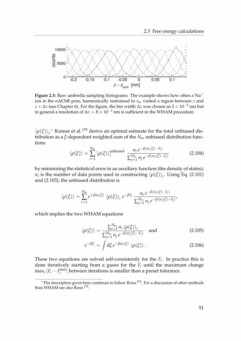
2.3 Free energy calculations
-0.2 -0.15 -0.1 -0.05 0 0.05 0.1z − zcom [nm]
0
5000
10000co
unts
Figure 2.3: Raw umbrella sampling histograms. The example shows how often a Na+
ion in the nAChR pore, harmonically restrained to z0, visited a region between z andz + ∆z (see Chapter 6). For the figure, the bin width ∆z was chosen as 2× 10⁻³ nm butin general a resolution of ∆z = 8× 10⁻³ nm is sufficient in the WHAM procedure.
〈ρ(ξ)〉i.∗ Kumar et al.175 derive an optimal estimate for the total unbiased dis-tribution as a ξ-dependent weighted sum of the Nw unbiased distribution func-tions
〈ρ(ξ)〉 =Nw
∑i=1〈ρ(ξ)〉unbiased
ini e−β(wi(ξ)−Fi)
∑Nwj=1 nj e−β(wj(ξ)−Fj)
(2.104)
by minimising the statistical error in an auxiliary function (the density of states);ni is the number of data points used in constructing 〈ρ(ξ)〉i. Using Eq. (2.101)and (2.103), the unbiased distribution is
〈ρ(ξ)〉 =Nw
∑i=1
e+βwi(ξ) 〈ρ(ξ)〉i e−βFini e−β(wi(ξ)−Fi)
∑Nwj=1 nj e−β(wj(ξ)−Fj)
,
which implies the two WHAM equations
〈ρ(ξ)〉 = ∑Nwi=1 ni 〈ρ(ξ)〉i
∑Nwj=1 nj e−β(wj(ξ)−Fj)
and (2.105)
e−βFi =∫
dξ e−βwi(ξ) 〈ρ(ξ)〉 . (2.106)
These two equations are solved self-consistently for the Fi. In practice this isdone iteratively starting from a guess for the Fi until the maximum changemaxi |Fi − Flast
i | between iterations is smaller than a preset tolerance.
∗The description given here continues to follow Roux174. For a discussion of other methodsthan WHAM see also Roux174.
51

2 Theory and Methods
-1 -0.5 0 0.5 1z [nm]
2
2.2
2.4
2.6
βW(z
) 10-1
10-2
10-3
10-4
10-5
10-6
10-8
(a) Flat constant PMF, generated fromβW(z) = 0
-1 -0.5 0 0.5 1z [nm]
1.5
2
2.5
3
3.5
4
βW(z
)
10-1
10-2
10-3
10-4
10-5
10-6
10-7
10-8
(b) Step function of height 2 kT PMF, gen-erated from βW(z) = 2Θ(z)
Figure 2.4: Test cases for the WHAM procedure and check of convergence. Input fortwo underlying PMFs was simulated and WHAM was used to recover the PMFs. Therecovered profiles are plotted for decreasing tolerances (in kT) of the self-consistentWHAM algorithm. The PMFs from WHAM are only determined up to a constant.
2.3.4 Umbrella sampling and WHAM in practice
The practical problems of applying umbrella sampling and WHAM to obtaina free energy profile in channels are briefly discussed. This includes tests ofthe WHAM procedure and a protocol to obtain W(z) from a combination ofequilibrium and umbrella sampled PMFs.
Test input The WHAM procedure is implemented in the program g wham(see Appendix D.2.5 for details). The implementation was tested by simulatinginput as if obtained by umbrella sampling a given PMF W(z) (using fakepmf,see Appendix D.3.2) and processing it with g wham. Results are shown inFig. 2.4 for increasing tolerances (in kT). A constant PMF poses no problemalthough a very small drift is visible. A step function of height 2 kT is resolvedprovided the tolerance is taken to be at least 10−5 kT. The step discontinuityitself has the correct height of 2 kT but the adjacent constant stretch of potentialis about 0.2 kT to low. Given the extreme case of a discontinuity, WHAM wasjudged to work satisfactory; for processing of MD umbrella sampling data thetolerance was chosen to be 10−5 or smaller.∗
∗WHAM is carried out in double precision (double variables) so the required tolerance isnot related to the loss of precision when only using float variables.
52
2.3 Free energy calculations
Matching umbrella and equilibrium PMF As pointed out before, the 1D PMFis not well defined outside the pore region. In particular, it is not possible to um-brella sample along z without confinement in x and y. One possibility is to addan artificial confining potential170 (and see Appendix D.3.1) whose influencecan later be removed from the PMF.∗ Here a less rigorous and conceptually sim-pler method was employed. The equilibrium density is always well sampled inthe bulk region and in the entrance (“mouth”) regions of the pore, which allowsto define a PMF that is accurate in bulk and mouth but is typically inaccurate inthe pore itself. Umbrella sampling, on the other hand, yields accurate results inthe mouth and the pore region, where lateral particle movements are bounded,but not in the bulk. Both PMFs should be accurate in the mouth region and asthey describe the same system one can match them to obtain a continuous PMF.This operation was carried out manually; errors associated with this procedureare estimated to be smaller than 0.5 kT, sometimes less than 0.1 kT if the matchis very good. The matching of the equilibrium PMF with the umbrella PMF alsoensures that absolute barrier heights (relative to the bulk) can be obtained.
Equilibration and drift correction Umbrella sampling in complex pores suchas the nAChR pore (Chapter 6) is complicated by the fact that—unlike in simplemodel pores—it is by no means clear what the PMF should look like. How-ever, if the density is sufficiently sampled during an equilibrium trajectory thenEq. (2.95) yields the PMF. A PMF obtained with umbrella sampling and WHAMcan then compared to the “true” PMF. For ions the barriers are too high in theclosed nAChR pore but water permeates rather freely, which is expressed in bar-riers less than 1.5 kT high (Fig. 2.5(a)). A water molecule was umbrella sampledin 101 windows for 1.5 ns in each window (see Section 6.2.4 and Tab. 6.2 onpage 133 for details). An initial part of length Teq of the umbrella sampled timeseries
(t, z(t) − zi(t)
)is discarded as equilibration time, with T remaining as
production data. As Fig. 2.5(a) shows, the influence of the equilibration phaseis moderate, and Teq = 0.5 ns appears to suffice for a converged PMF.
A more serious problem is a systematic “drift” or linear shift in the umbrellaPMF compared to the equilibrium PMF (which was observed in many but notall other PMFs that were analysed in this work). For symmetric problems suchas the model pores, very good agreement between the PMFs was achieved bysymmetrizing the PMF (see Fig. 5.4 on page 115 and Section 5.2.2). This is notpossible for asymmetric pores so it was decided to apply a “drift correction”. Afunction
∆drift(z) = λz (2.107)
∗Confining potentials were considered but tests did not show a significant advantage overthe method that was finally used.
53

2 Theory and Methods
-3 -2 -1 0 1 2 3
z [nm]
-3
-2
-1
0
1
2
3
4
PM
F [k
T]
equilibrium0.1 ns + 1.4 ns0.5 ns + 1.0 ns1.0 ns + 0.5 ns
(a) Influence of equilibra-tion time and sampling time,Teq+T.
-3 -2 -1 0 1 2 3
z [nm]
-3
-2
-1
0
1
2
3
4
PM
F [k
T]
equilibriumWHAM(0.5 ns+1.0 ns)WHAM,drift corrected
(b) PMF, drift corrected byW(z)→W(z) + ∆drift(z).
Figure 2.5: Equilibration time and drift correction of the PMF for water in nAChR. (a)The influence of the equilibration phase on the PMF is comparatively small. (b) Goodagreement with the PMF from the equilibrium density is only obtained after adding acorrection ∆drift(z) = 0.614 kT nm−1 × z for “drift” in the WHAM procedure.
with the adjustable parameter λ is added to W(z) so that the corrected um-brella PMF W(z) + ∆drift(z) can be matched to the equilibrium PMF. Althoughsimilar “hysteresis” effects have been reported176 and attributed to correlationsin subsequent starting configurations, this is not likely to be the case here asthe starting positions in adjacent windows tend to be from different times of theequilibrium trajectory and are therefore uncorrelated. It probably rather reflectsthe fact that the WHAM procedure integrates histogram data drom the wholerange and can be somewhat sensitive to incomplete sampling in the outermostbins. In principle the PMF could be constrained to be the same at either end ofthe range because no potential difference occurs. In practice, this systematic er-ror can be corrected for by comparison (or calibration) to the equilibrium PMFas was done here.
2.4 Poisson-Boltzmann electrostatics
Molecular dynamics simulations are very CPU intensive. An estimate for bind-ing energies or the PMF for an ion in a pore can also be obtained from a static
54

2.4 Poisson-Boltzmann electrostatics
structure. In this approach, interactions are reduced to electrostatic contribu-tions, i.e. only the static or “fixed” charge distribution of a protein
ρf(x) = ∑i
qiδ(x− xi) (2.108)
interacts with another protein or an ion. Dynamic and hence entropic effects arenot included. The solvent is treated as a continuum so the size of the problem isreduced considerably, and because averaging effects can be incorporated, suchas the rapid re-orientation of the strong water dipoles, which is responsible forthe high dielectric constant of water. Water is treated as a continuous mediumwith dielectric constant εw ≈ 78.5 whereas proteins are given 2 ≤ εp ≤ 16.Mobile ions in solution are treated in Debye-Huckel theory177 as continuousdistributions
ρ+(x) = +z+e n+(∞) e−β z+e φ(x)
ρ−(x) = −z−e n−(∞) e+β z−e φ(x),(2.109)
where z± is the valence and n±(∞) the bulk concentration of the ions. Thedensity depends on the electric potential φ(x) through the Boltzmann factor;φ(x) is generated by the fixed charges (2.108) and by the mobile charges (2.109)themselves. Inserting the total charge ρ := ρf + ρ+ + ρ− into Poisson’s equation
−∇ · [ε(x)∇φ(x)] =ρ(x)
ε0(2.110)
yields the Poisson-Boltzmann equation.82 For a salt with symmetric charges onthe ions (valence z := z+ = z−, e.g. NaCl z = 1) and bulk concentrationn0 = n±(∞) it can be written178,179
−∇ · [ε(x)∇ · φ(x)] = −2zen0χ(x)ε0
sinh[βzeφ(x)] +ρf
ε0. (2.111)
The shape function χ(x) is 1 in the solvent and 0 in the protein; it ensures thatthe effect of the mobile ions only applies to the region accessible to the ions.Similarly, ε(x) equals εp in the protein interior and εw in the region accessibleto solvent.
For zeφ(x) kT the non-linear term sinh[βzeφ(x)] can be approximated byβzeφ(x) so that Eq. (2.111) becomes the linearised Poisson-Boltzmann equation,
−∇ · [ε(x)∇ · φ(x)] = −κ2(x)φ(x) +ρf
ε0with (2.112)
κ2(x) :=2βe2n0z2χ(x)
ε0=
2βe2 Iχ(x)ε0
. (2.113)
55
2 Theory and Methods
For electrolytes of differing valence zi, the term n0z2 can be replaced by theionic strength I := 1
2 ∑i niz2i of all ionic species.∗ In the electrolyte region where
χ(x) = 1 and ε(x) = εw, κ2 is related to the Debye screening length λ,
εwκ−2 = λ2 =εwε0
2βe2 I,
which is the thickness of electrolyte solution that reduces the potential of a pointcharge by a factor of 1/e;82 for I = 0.1 mol · l−1 NaCl, λ = 0.962 nm.
Electrostatic free energy For the linear Poisson-Boltzmann equation (2.112)the total electrostatic energy is180
∆Gel = 12
∫d3x ρf(x) φ(x); (2.114)
it is the free energy required to charge the system (the fixed charges) in thepresence of the mobile ions. The electrostatic binding energy of an explicit ion ina protein channel at subsequent positions z along the pore axis (or electrostaticPMF) can be calculated as
∆GB(z) = ∆GelPI(z)− ∆Gel
I − ∆GelP . (2.115)
∆GelPI denotes the electrostatic energy of the system comprising the pore and the
ion, located at position z. ∆GelI is the electrostatic energy of an ion in the solvent.
In order to minimise artifacts due to the calculation algorithm, ∆GelI (z) is calcu-
lated for every position z of the ion in the channel. ∆GelP is the total electrostatic
energy of the pore/slab system immersed in high dielectric solvent. The explicition is modelled as a spherical cavity of the same dielectric as the protein† witha radius (Born radius) that reproduces experimental solvation energies.181
Poisson-Boltzmann solver In order to solve the Poisson-Boltzmann equa-tion (2.111) or (2.112) for arbitrary shapes χ(x) and ε(x) the problem is dis-cretized on a grid. For the Born profile calculations in Chapter 5 and 6, theprogram apbs179 was used, which uses a finite elements algorithm for discret-ization.182,183 For the calculation of the protonation states, i.e. the pKa s,184,185
of the residues in the nicotinic acetylcholine receptor transmembrane domain(Chapter 6), DelPhi186 was used, which employs a finite difference scheme.
∗If the ionic strength is given in mol · l−1 instead of m−3 then it needs to be converted tom−3: I/(mol · l−1) · 103 NA = I/m−3 with Avogadro’s constant NA = 6.02214179× 10²³ mol−1.†For the ion itself a dielectric of ε = 1 would be more appropriate but the program apbs is
not yet capable of calculating multiple low-dielectric regions.
56
3 The surprising behaviour of confinedwater
Water confined to short (L = 0.8 nm) hydrophobic pores (radius0.35 nm ≤ R ≤ 1.0 nm) is studied by atomistic molecular dynam-ics simulations. The water density in the pore fluctuates on a nano-second time scale between a liquid and vapour filled pore. Theseliquid-vapour oscillations can be explained as capillary evapora-tion alternating with capillary condensation, driven by local pres-sure fluctuations in the water outside the pore. The free energylandscape shows how a metastable liquid state gradually developswith increasing radius. For radii larger than ca. 0.55 nm the liquidbecomes the globally stable state and the vapour state vanishes.One dimensional confinement affects the dynamic behaviour ofthe water molecules and increases the self diffusion by a factor oftwo to three compared to bulk water. Permeabilities for the narrowpores are of the same order of magnitude as for biological waterpores. Water flow is not continuous but occurs in bursts.
Channel and transporter proteins control flow of water, ions and other solutesacross cell membranes. In recent years several channel and pore structures havebeen solved at near atomic resolution16,30,51,55,69,71 which together with threedecades of physiological data12 and theoretical and simulation approaches95
allow us to describe transport of ions, water or other small molecules at a mo-lecular level. Water plays a special role here: it either solvates the inner surfacesof the pore and the permeators (for example, ions and small molecules like gly-cerol), or it is the permeant species itself as in the aquaporin family of waterpores13,187,188 or in the bacterial peptide channel gramicidin A (gA), whose wa-ter transport properties are well studied.189–191 Thus, a better characterisationof the behaviour of water would improve our understanding of the biologicalfunction of a wide range of transporters. The remarkable water transport prop-erties of aquaporins—water is conducted through a long (ca. 2 nm) and narrow(ca. 0.3 nm diameter) pore at bulk diffusion rates while at the same time protonsare strongly selected against—are the topic of recent simulation studies.72,192
The shape and dimensions of biological pores and the nature of the pore lin-ing atoms are recognised as major determinants of function. How the beha-viour of water depends on these factors is far from understood.9 Water is not a
57
3 The surprising behaviour of confined water
simple liquid due to its strong hydrogen bond network. When confined to nar-row geometries like slits or pores it displays an even more diverse behaviourthan already shown in its bulk state.193,194
3.1 Water in pores
A biological channel can be crudely approximated as a “hole” through a mem-brane. Earlier molecular dynamics (MD) simulations showed pronouncedlayering effects and a marked decrease in water self diffusion in infinite hy-drophobic pore models.195,196 Hummer et al.197, Beckstein et al.62, and Allenet al.198 observed that water in finite narrow hydrophobic pores exhibited adistinct two-state behaviour. The cavity was either filled with water at approx-imately bulk density (liquid-like) or it was almost completely empty (vapour-like). Similar behaviour was seen in Gibbs ensemble Monte Carlo simulations(GEMC) in spherical1 and cylindrical pores.199
In our previous simulations62∗ we explored model pores of the dimensionsof the gating region of the nicotinic acetylcholine receptor nAChR.59† Hydro-phobic pores of radius R ≥ 0.7 nm were filled during the whole simulationtime (up to 6 ns) whereas narrow ones (R ≤ 0.4 nm) were permanently empty.Changing the pore lining from a hydrophobic surface to a more hydrophilic (po-lar) one rendered even narrow pores water—and presumably ion—conducting.At intermediate radii (0.4 nm < R < 0.7 nm) the pore-water system was verysensitive to small changes in radius or character of the pore lining. In a biolo-gical context, a structure close to the transition radius would confer the highestsusceptibility to small conformational rearrangements (i.e. gating) of a channel.
The previous short-time scale simulations62 gave a tantalising hint at inter-esting emerging phenomena at longer time scales. In this chapter considerablylonger simulations are presented (> 50 ns instead of 1 ns) in order to explorethe longer timescale behaviour of the water-pore system. Starting from the ob-served oscillations in water density (Fig. 3.1 on the facing page) we analyse thekinetics and the free energy of the system. We compare the water transportproperties of the pores to experimental and theoretical data. First, however, welook at the behaviour of water in the simplest inhomogeneous system, namelyat a planar hydrophobic surface. So we are able to pinpoint the effect of the
∗The simulations reported in Beckstein et al.62 were comparatively short (typically, only 1 nsper simulation) and although the main conclusions are still valid, more detailed and extensivesimulations are the subject of this and the following chapter. Therefore, the results from our pre-vious paper are not explicitly shown here; the conclusions arising from the material presentedhere recapitulate and extend the results of the previous paper.†Note that at the time (2001/2002) the atomic resolution structure of the nAChR transmem-
brane domain29 was not known yet.
58

3.2 Methods
Figure 3.1: Oscillating water density in model pores of increasing pore radius R. Thewater density n(t) (in units of the bulk water density n0) over the simulation time showsstrong fluctuations on a greater than ns time scale (50 ps moving average smoothing).Two distinctive states are visible: open at approximately n0 (liquid water), and closedwith very few or no water in the pore (water vapour).
higher degree of confinement conferred by the cylindrical pores compared tothe less confining planar surface whilst using the bulk system (“neat water”) asa reference for both. In this sense, a planar surface can be seen as the limitingcase of a pore with an infinite radius.
3.2 Methods
For completeness, some of the methodological aspects, that were already men-tioned in Chapter 2, are repeated here, together with the parameters of the MDsimulations that were used for the calculations of this chapter.
59
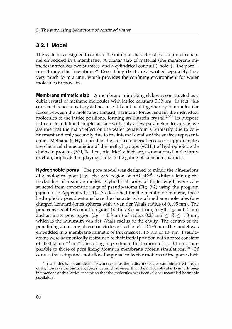
3 The surprising behaviour of confined water
3.2.1 Model
The system is designed to capture the minimal characteristics of a protein chan-nel embedded in a membrane: A planar slab of material (the membrane mi-metic) introduces two surfaces, and a cylindrical conduit (“hole”)—the pore—runs through the “membrane”. Even though both are described separately, theyvery much form a unit, which provides the confining environment for watermolecules to move in.
Membrane mimetic slab A membrane mimicking slab was constructed as acubic crystal of methane molecules with lattice constant 0.39 nm. In fact, thisconstruct is not a real crystal because it is not held together by intermolecularforces between the molecules. Instead, harmonic forces restrain the individualmolecules to the lattice positions, forming an Einstein crystal.200∗ Its purposeis to create a defined simple surface with only a few parameters to vary as weassume that the major effect on the water behaviour is primarily due to con-finement and only secondly due to the internal details of the surface represent-ation. Methane (CH4) is used as the surface material because it approximatesthe chemical characteristics of the methyl groups (–CH3) of hydrophobic sidechains in proteins (Val, Ile, Leu, Ala, Met) which are, as mentioned in the intro-duction, implicated in playing a role in the gating of some ion channels.
Hydrophobic pores The pore model was designed to mimic the dimensionsof a biological pore (e.g. the gate region of nAChR59), whilst retaining thetractability of a simple model. Cylindrical pores of finite length were con-structed from concentric rings of pseudo-atoms (Fig. 3.2) using the programpgeom (see Appendix D.1.1). As described for the membrane mimetic, thesehydrophobic pseudo-atoms have the characteristics of methane molecules (un-charged Lennard-Jones spheres with a van der Waals radius of 0.195 nm). Thepore consists of two mouth regions (radius RM = 1 nm, length LM = 0.4 nm)and an inner pore region (LP = 0.8 nm) of radius 0.35 nm ≤ R ≤ 1.0 nm,which is the minimum van der Waals radius of the cavity. The centres of thepore lining atoms are placed on circles of radius R + 0.195 nm. The model wasembedded in a membrane mimetic of thickness ca. 1.5 nm or 1.9 nm. Pseudo-atoms were harmonically restrained to their initial position with a force constantof 1000 kJ mol−1 nm−2, resulting in positional fluctuations of ca. 0.1 nm, com-parable to those of pore lining atoms in membrane protein simulations.201 Ofcourse, this setup does not allow for global collective motions of the pore which∗In fact, this is not an ideal Einstein crystal as the lattice molecules can interact with each
other; however the harmonic forces are much stronger than the inter-molecular Lennard-Jonesinteractions at this lattice spacing so that the molecules act effectively as uncoupled harmonicoscillators.
60

3.2 Methods
(a) Van der Waals surface
RM
R
LP
LM
z
RM = 1.0 nmLM = 0.4 nmLP = 0.8 nm
(b) Schematic
Figure 3.2: Model pore system. (a) The pore model consists of methane pseudo-atomsof van der Waals radius 0.195 nm. The pore (cyan) is embedded in a membrane mimeticslab (gold). Pore and slab consist of the same kind of methane atoms. (b) The geometryof the mouth region (length LM and radius RM) and the length LP of the pore have beenkept fixed throughout the calculations in this chapter but the pore radius R ≡ RP wasvaried. A water molecule is drawn to scale.
are necessary in real proteins for gating to occur. However, here the aim is not tosimulate these large scale motions but to investigate the behaviour of water ina environment characteristic of either the open or the closed state. Because thetime scale of gating motions is on the millisecond time scale12 but solvent re-arranges on much shorter time scales (pico- to nanoseconds) our simplificationsappear to be reasonable ones.
3.2.2 Simulation Details
MD simulations were performed with gromacs version 3.0.5 (Ref. 127) and theSPC water model.132 Parameters for the unified methane atoms are describedin Section 2.2.3 on page 38. The integration time step was 2 fs and coordinateswere saved every 2 ps. With periodic boundary conditions, long range elec-trostatic interactions were computed with a particle mesh Ewald method (realspace cutoff 1 nm, grid spacing 0.15 nm, 4th order interpolation164,165) whilethe short ranged van der Waals forces were calculated within a radius of 1 nm.The neighbour list (radius 1 nm) was updated every 10 steps. Weak coupling
61
3 The surprising behaviour of confined water
algorithms166 were used to simulate at constant temperature (T = 300 K, timeconstant 0.1 ps) and pressure (pz = 1 bar, compressibility 4.5 × 10⁻⁵ bar−1,time constant 1 ps) where the box dimensions in the plane of the membranewere held fixed.
Membrane mimetic slab A box (size 6 nm× 6 nm× 4.6 nm) with a membranemimetic of thickness 1.2 nm and altogether 3 nm of SPC water was simulated for20 ns. The system contained 675 methane molecules and 3910 water molecules.
Hydrophobic pores For the simulations of water in the hydrophobic poremodels, the pore/slab system was solvated with SPC water, forming a simu-lation cell with lengths in x and y of 6 nm (or 3.9 nm for the 80 ns simulationof the R = 0.35 nm pore). The length in z was 4.6 nm in both cases (ensuringbulk-like water behaviour far from the membrane mimetic). The large (small)system contained about 700 (300) methane pseudo-atoms and 4000 (1500) SPCwater molecules. Simulation times T ranged from 52 ns to 80 ns (altogether460 ns).
Bulk water Bulk properties of SPC water were obtained from simulations ofneat water (i.e. just water) in a cubic cell of length 3 nm (895 molecules) withisotropic pressure coupling at 300 K and 1 bar for 5 ns.
3.2.3 Analysis
To a certain degree, analysis of simulations is similar to analysis of experimentaldata though it differs in that one actually has detailed knowledge of all particlesinvolved because the positions (and sometimes velocities) are recorded in thetrajectory over time. But this level of detail is overwhelming and does not lenditself to facilitating a deeper understanding of the simulated system. So the taskis to define and “measure” (i.e. compute) meaningful observables in order tomake sense of the intricate dance that is performed by the atoms.
Time courses and density For the density time courses (Fig. 3.1 on page 59)the pore occupancy N(t), i.e. the number of water molecules in the pore cavity(a cylinder of height LP = 0.8 nm containing the pore lining atoms) was countedwith g count (Appendix D.2.1). The density n(t) is given by N(t) divided by thewater-accessible pore volume
V = LP πR2eff (3.1)
62
3.2 Methods
and normalised to the bulk density of SPC water at 300 K and 1 bar (n0 =
53.67 ± 0.03 mol · l−1).∗ The effective pore radius for all pores is Reff = R −δR. Choosing δR = 0.03 nm fixes the density 〈N〉/V in the (most bulk-like)R = 1.0 nm-pore at the value calculated from the radial density, R−1
0
∫ R00 n(r) dr,
where R0 = 1.05 nm is the radius at which n(r) vanishes (see Section 2.1.4 onpage 28).
The density n(x) was determined on a grid of cubic cells with spacing0.05 nm, using g ri3Dc (Appendix D.2.3). Two- and one-dimensional dens-ities were computed by integrating out the appropriate coordinate(s) witha ri3Dc. Because an equilibrium MD simulation samples states according tothe Boltzmann factor, the potential of mean force (PMF) of a water molecule isrelated to the water density n(x) by
βW(x) = − lnn(x)n0
+ β(W0 − µ0) (2.94)
(see also Section 2.3.1 on page 46). W0−µ0 is not determined in our simulations,and because it is generally different for different systems (e.g. pores of differentradii) we normally cannot compare the position of different W(x; R) relative toeach other.† We can identify the PMF W(x) of Eq. (2.94) with the constrainedgrand potential Ω(x), as detailed in the next section.
Free energy density We consider the free energy of the fluid in the pore. Tothis end we imagine a subsystem of the full simulation box which contains thepore and a buffer region. Because the full system is simulated at constant pres-sure (and temperature), the water density and thus the chemical potential nearthe pore entrance is essentially fixed. Thus the fluid in the pore is most conveni-ently treated in the grand canonical ensemble202 (fixed temperature, volume,and chemical potential, see Section 2.1 on page 17).‡ Hence the free energy isthe grand potential. The number of particles N in the subsystem fluctuates, butthe average is fixed by µ. In order to distinguish different phases of the fluidin the pore we introduce the pore occupancy N∗, the number of particles in thepore of volume V = πR2L. Then the density in the pore region n∗ := N∗/V∗The symbol n is used as a density in a fairly wide sense, and interchangeably denotes
number density or concentration, or mass density; for SPC water n0 = 0.997× 10³ kg ·m−3.†The situation is analogous to the case of umbrella sampling (cf. Section 2.3.2) where a
procedure has to be found to join neighbouring histograms. WHAM (Section 2.3.3) preciselydetermines the relative free energy offsets by a histogram reweighting technique.‡In Ref. 96 we took the free energy to be the Helmholtz free energy but it was subsequently
pointed out by Allen et al.202 that the most appropriate thermodynamic potential is the grandpotential where the number of water molecules in the pore takes the role of a reaction coordin-ate. Similarly, Hunter III and Reinhardt203 use the average volume per particle v := V/N asthe order parameter in a constrained free energy of the isothermal-isobaric ensemble.
63
3 The surprising behaviour of confined water
is a suitable order parameter. (n∗ is the inverse of the average volume per watermolecule v = V/N∗ which could also be used as an order parameter.203) Weare interested in the free energy as a function of the order parameter, i.e. theconstrained free energy
βΩ(n∗) = − ln Ξ(n∗), (3.2)
(cf. Section 2.1.3 on page 27) where the grand canonical partition function (2.12)is constrained to values which correspond to a pore filled with fluid at densityn∗,
Ξ(n∗) = Trn∗(xi)=n∗
e−β(H−µN). (3.3)
n∗(xi) is the density in the pore for a particular configuration of moleculesxi. The simulations yield the probability p(n∗) to observe the subsystem in astate with fluid density n∗. Hence the constrained free energy can be calculatedfrom the simulation data as
βΩ(n∗) = − ln p(n∗) + βΩ. (3.4)
and transformed into a free energy density
ω(n∗) ≡ ω(T, µ; n∗) = Ω(T, V, µ; n∗)/V, (3.5)
A sixth order polynomial in n∗ was least-square fitted to βω(n∗), except forthe pores with radii 0.15 nm, 0.2 nm, and 1.0 nm for which a cubic regressionsufficed. The βω(n∗) curves obtained for different radii R from the simulationsare only determined within the additive constant Ω, which is the free energy ofthe pore system βΩ = − ln V
∫ ∞0 dn∗ Ξ(n∗).
For the free energy density Eq. (3.5) we can show that all curves coincide forn∗ = 0, which effectively describes the vapour state. Let ω be the free energydensity in the pore region and ω′ = −p′ the free energy density in the adjacentbuffer and bulk regions. In equilibrium these densities have the same valueω = ω′, and, using the model Eq. (4.4), which will be introduced in detail in thenext chapter (see page 90), this simply expresses mechanical equilibrium acrossthe meniscus,
−p + V−1(
2πRLγ f w(n∗) + 2πR2γ f l(n∗))= −p′.
The surface tensions γ between the fluid f in the pore (vapour or liquid) andthe wall w or the liquid l in the buffer/bulk regions vary with the density n∗
of the fluid; the dependency on temperature is not explicitly shown. With theintroduction of the aspect ratio of the pore η = R/L, the free energy density inthe pore depends on n∗ as
ω(n∗) = −p′ − 2L−1(
η−1γ f w(n∗) + γ f l(n∗))
. (3.6)
64
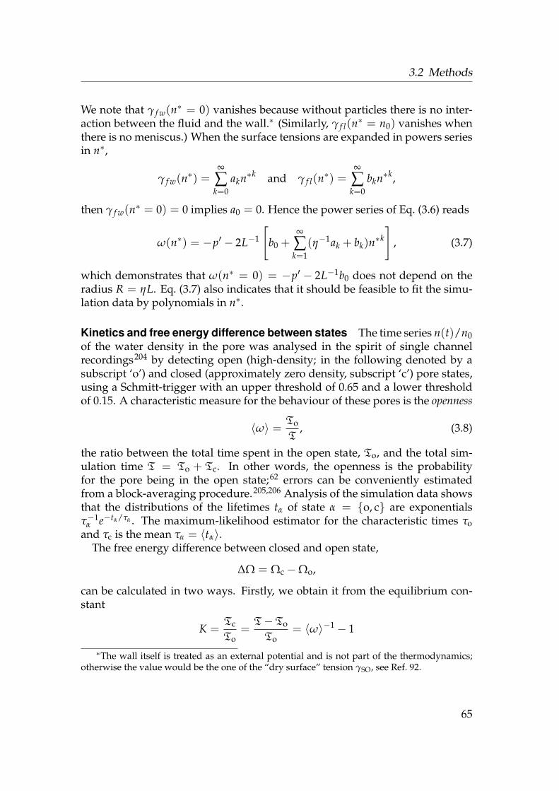
3.2 Methods
We note that γ f w(n∗ = 0) vanishes because without particles there is no inter-action between the fluid and the wall.∗ (Similarly, γ f l(n∗ = n0) vanishes whenthere is no meniscus.) When the surface tensions are expanded in powers seriesin n∗,
γ f w(n∗) =∞
∑k=0
akn∗k and γ f l(n∗) =∞
∑k=0
bkn∗k,
then γ f w(n∗ = 0) = 0 implies a0 = 0. Hence the power series of Eq. (3.6) reads
ω(n∗) = −p′ − 2L−1
[b0 +
∞
∑k=1
(η−1ak + bk)n∗k
], (3.7)
which demonstrates that ω(n∗ = 0) = −p′ − 2L−1b0 does not depend on theradius R = ηL. Eq. (3.7) also indicates that it should be feasible to fit the simu-lation data by polynomials in n∗.
Kinetics and free energy difference between states The time series n(t)/n0of the water density in the pore was analysed in the spirit of single channelrecordings204 by detecting open (high-density; in the following denoted by asubscript ‘o’) and closed (approximately zero density, subscript ‘c’) pore states,using a Schmitt-trigger with an upper threshold of 0.65 and a lower thresholdof 0.15. A characteristic measure for the behaviour of these pores is the openness
〈ω〉 = To
T, (3.8)
the ratio between the total time spent in the open state, To, and the total sim-ulation time T = To + Tc. In other words, the openness is the probabilityfor the pore being in the open state;62 errors can be conveniently estimatedfrom a block-averaging procedure.205,206 Analysis of the simulation data showsthat the distributions of the lifetimes tα of state α = o, c are exponentialsτ−1
α e−tα/τα . The maximum-likelihood estimator for the characteristic times τoand τc is the mean τα = 〈tα〉.
The free energy difference between closed and open state,
∆Ω = Ωc −Ωo,
can be calculated in two ways. Firstly, we obtain it from the equilibrium con-stant
K =Tc
To=
T− To
To= 〈ω〉−1 − 1
∗The wall itself is treated as an external potential and is not part of the thermodynamics;otherwise the value would be the one of the “dry surface” tension γSO, see Ref. 92.
65

3 The surprising behaviour of confined water
of the two-state system openclosed as
β ∆Ωkin = − ln K. (3.9)
Secondly, ∆Ω is determined from p(N∗) as the ratio between the probabilitythat the pore is in the closed state and the probability for the open state,
β ∆Ωeq = − lnPc
Po= − ln
∑N∗≤N‡ p(N∗)∑N∗>N‡ p(N∗)
. (3.10)
The definition of state used here is independent of the kinetic analysis. It onlydepends on N‡, the pore occupancy in the transition state, the state of lowestprobability between the two probability maxima that define the closed and openstate. Of course, Eq. (3.10) is only applicable if both a liquid and a vapour stateexist; Eq. (3.9) can be formally applied even if there is only one stable state. Therelationship involving K can be inverted to describe the openness in terms of∆Ω(R),
〈ω(R)〉 = 11 + exp[−β ∆Ω(R)]
. (3.11)
Self-diffusion coefficient The three Cartesian components of the self-diffusion coefficient of water are calculated from the Einstein relations112⟨(
xi(t)− xi(t0))2⟩= 2Di (t− t0) (3.12)
(which is understood to be exact in the limit t → ∞). We can rewrite (3.12) forthe diffusion in space as⟨(
x(t)− x(t0))2⟩= 2 Tr D (t− t0), with Dij := Diδij, (3.13)
where the diffusion constant is now a diagonal Cartesian tensor D.∗ This for-mulation is motivated by a generalisation of Fick’s law for the current
j(x, t) = −D∇n(x, t) (3.14)
and the continuity equation
∂n(x, t)∂t
−∇ ·D∇n(x, t) = 0 (3.15)
∗Tr is the standard trace operation on tensors, TrD = ∑3i=1 Dii. The tensor transformation
properties follow from Eq. (3.14).
66
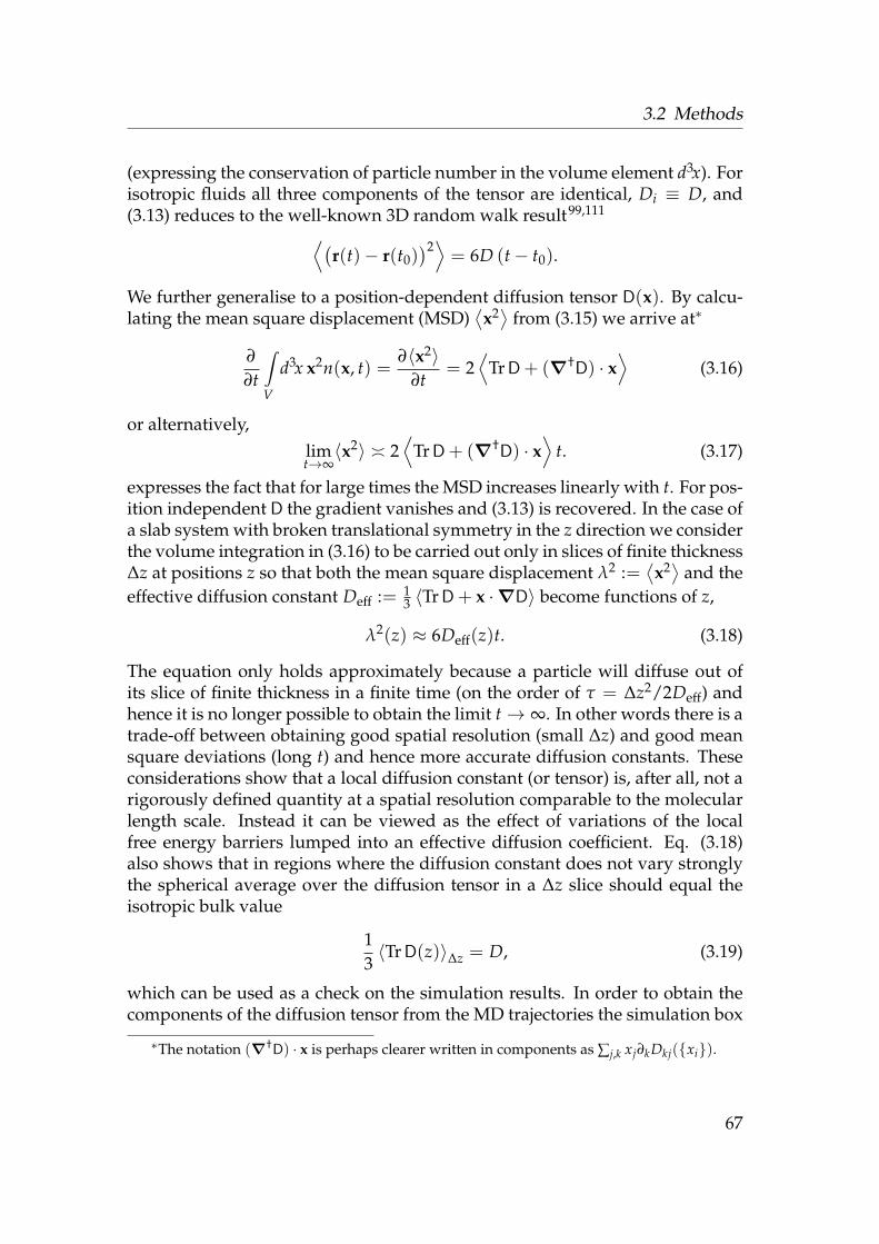
3.2 Methods
(expressing the conservation of particle number in the volume element d3x). Forisotropic fluids all three components of the tensor are identical, Di ≡ D, and(3.13) reduces to the well-known 3D random walk result99,111⟨(
r(t)− r(t0))2⟩= 6D (t− t0).
We further generalise to a position-dependent diffusion tensor D(x). By calcu-lating the mean square displacement (MSD)
⟨x2⟩ from (3.15) we arrive at∗
∂
∂t
∫V
d3x x2n(x, t) =∂〈x2〉
∂t= 2
⟨Tr D + (∇†D) · x
⟩(3.16)
or alternatively,limt→∞〈x2〉 2
⟨Tr D + (∇†D) · x
⟩t. (3.17)
expresses the fact that for large times the MSD increases linearly with t. For pos-ition independent D the gradient vanishes and (3.13) is recovered. In the case ofa slab system with broken translational symmetry in the z direction we considerthe volume integration in (3.16) to be carried out only in slices of finite thickness∆z at positions z so that both the mean square displacement λ2 :=
⟨x2⟩ and the
effective diffusion constant Deff := 13 〈Tr D + x ·∇D〉 become functions of z,
λ2(z) ≈ 6Deff(z)t. (3.18)
The equation only holds approximately because a particle will diffuse out ofits slice of finite thickness in a finite time (on the order of τ = ∆z2/2Deff) andhence it is no longer possible to obtain the limit t→ ∞. In other words there is atrade-off between obtaining good spatial resolution (small ∆z) and good meansquare deviations (long t) and hence more accurate diffusion constants. Theseconsiderations show that a local diffusion constant (or tensor) is, after all, not arigorously defined quantity at a spatial resolution comparable to the molecularlength scale. Instead it can be viewed as the effect of variations of the localfree energy barriers lumped into an effective diffusion coefficient. Eq. (3.18)also shows that in regions where the diffusion constant does not vary stronglythe spherical average over the diffusion tensor in a ∆z slice should equal theisotropic bulk value
13〈Tr D(z)〉∆z = D, (3.19)
which can be used as a check on the simulation results. In order to obtain thecomponents of the diffusion tensor from the MD trajectories the simulation box
∗The notation (∇†D) · x is perhaps clearer written in components as ∑j,k xj∂kDkj(xi).
67

3 The surprising behaviour of confined water
was stratified perpendicular to the pore axis or slab normal; the central layer ofthickness ∆z = L contained the whole pore region. During the simulation timeT the MSD of water molecules in a given layer was accumulated for 10 ps andafter discarding the first 2 ps, a straight line was fit to the MSD to obtain Di.These diffusion coefficients were averaged in each layer for the final result.
Water current density The current density (flux per area) was calculated asj0 = Φ0/A from the equilibrium flux Φ0 = M/T with the total number ofpermeant water molecules M and the effective pore cross section A = πR2
eff forpores or A = LxLy for the bulk case, i.e. a simulation box of water with periodicboundary conditions. Permeant water molecules were defined as those whosepore entrance and exit z-coordinate differed (see Appendix D.2.2 for details). Inaddition, distributions of permeation times were computed.
3.3 Results and Discussion
Before investigating water in cylindrical pores in Section 3.3.2 it is worthwhileto look at the simplest inhomogeneous system: a planar surface in contact withliquid water. This will later allow us to compare the effect of different degreesof confinement. In cylindrical pores water is more strongly confined than neara surface. The former restricts movement of water molecules in the xy-plane(with the pore axis pointing along z) whereas the latter only restricts movementin one half-space along −z (if the surface normal is taken to be parallel to +z).
3.3.1 Water near a hydrophobic surface
As described in Section 3.2.1, the hydrophobic surface comprises a crystal-likeslab of methane molecules. These molecules (represented as united atoms withimplicit hydrogens) oscillate about their equilibrium position with an RMSD ofabout 0.1 nm. The surface normal is parallel to the z direction, and all propertiesof interest are predominantly a function of z.
Density variations: Layering Simple, non-associating fluids like liquid ar-gon or the theoretician’s favourites, the hard sphere or the Lennard-Jonesfluid,101 exhibit a strongly layered structure near a repulsive or weakly attract-ive surface194,207 with spatial oscillations in density which can span almost oneorder of magnitude. Associating liquids like water tend to show weaker layer-ing (about 20% to 50% variation in density compared to the bulk value) as seenin simulations;84,208–216 experimental evidence by surface force apparatus meas-urements,217,218 atomic force microscopy (J. Pethica, personal communication),
68

3.3 Results and Discussion
0.05
0.10
0.20
0.30
0.40
0.50
0.60
0.70
0.80
0.90
1.00
1.10
1.20
1.30
1.40
Figure 3.3: Water density near a hydrophobic surface. The density is averaged over they direction. Weak layering is visible near the membrane mimetic slab. The interlayerdistance is about 0.3 nm. The graph shows an average over a simulation time T = 20 ns;note that even after this comparatively long time the average density in the bulk hasnot completely converged (compare to the uniform density in Fig. 5.5 on page 116 overT = 100 ns). The density is in units of SPC bulk water n0 = 0.997× 10³ kg ·m−3 atT = 300 K and P = 1 bar. See also the one-dimensional density profile in Fig. 3.4 on thefollowing page.
and neutron diffraction219 is indicative of surface layers near different kinds ofsurface. As shown in Fig. 3.3 and the bottom panel of Fig. 3.4 on the next pagewater near a hydrophobic slab shows marked layering. The 2D density showsthat the influence of the surface roughness on the density is not large and onlyaffects water directly adjacent to the surface. Two layers are visible, with thepeak height not exceeding 1.2n0 (where n0 = 0.997× 10³ kg ·m−3 denotes thedensity of SPC water at standard conditions). Between the first water layer andthe slab surface there is a region of very low water density which is knownas the depletion layer.90,94,215,216,220 Its thickness of ca. 0.2 nm is in accord withother simulation studies of explicit water near hydrophobic surfaces.215,216 Thethickness of one water layer (as measured by the peak to peak distance betweenthe two layers) is about 0.3 nm, which is only slightly larger than the positionof the first peak in the oxygen-oxygen radial distribution function in bulk waterat 0.28 nm. The influence of the wall, as far as the density is concerned, doesnot extend farther than two to three water layers, i.e. about 1 nm; this wasalready noted in early MD simulations208,209 but at much shorter simulationtimes (72 ps). The range of layering effects suggests that the minimum thick-
69

3 The surprising behaviour of confined water
0.5
1
1.5
D/D
bulk
DxDy
Dz
0 0.5 1 1.5 2 2.5 3 3.5 4 4.5z (nm)
00.5
1
1.5
n(z)
/nbu
lk
Tr D/3
Figure 3.4: Diffusion coefficients of water near a hydrophobic surface. Top panel: Dif-fusion of SPC water molecules is measured in directions x and y parallel to the surfaceand in z perpendicular to it. Di are normalised to the value of the isotropic diffusioncoefficient of SPC water, D0 = 4.3 nm2 · ns−1 at T = 300 K and P = 1 bar. The isotropicaverage 1
3 TrD = 13 (Dx + Dy + Dz) is plotted as a check (see text). Error bars indicate
one standard deviation. Vertical lines show the van der Waals surface of the slab. Bot-tom panel: The one dimensional density profile n(z) shows weak layering and a 0.2 nmdepletion zone (n0 = 0.997× 10³ kg ·m−3).
ness of the water region around a solute should be larger than 1 nm so thatthe water at the edge of the simulation box has bulk characteristics. It shouldbe noted that water close to a surface which is fluid rather than crystalline doesnot exhibit pronounced layering as was observed by analysis of water near lipidmembranes and octane slabs (J. D. Faraldo-Gomez, personal communication).Presumably, the movements of the surface disrupt or smear out the layering,which is not too surprising as the difference in density of 20% relates to a freeenergy of layer stabilization of about β−1 ln 1.2 ≈ 0.2 kT (cf. Eq. (2.94)). This en-ergy can be easily overcome by fluctuations in the liquid-liquid interface. (Thefluctuations are capillary waves, which have a typical energy of 1 kT.221,222)However, the density is only one property, although a rather important one asfar as equilibrium properties are concerned. For dynamical properties, the dif-fusion coefficient should be a good indicator of the influence of the surface onthe liquid.
70

3.3 Results and Discussion
Figure 3.5: Snapshots of permeant watermolecules in a R = 0.55 nm pore as itswitches from the open to the closed state.z-coordinates of the water oxygen atomsare drawn every 2 ps. The mouth and poreregion are indicated by horizontal brokenand solid lines. Five trajectories are shownexplicitly. The white water molecule per-meates the pore within 54 ps whereas theblack one only requires about 10 ps.
Dynamics The components of the self-diffusion coefficient tensor are shownin Fig. 3.4 as functions of z. The translational symmetry of the system isbroken normal to the surface. Accordingly Dz, and Dx and Dy only varywith z. The components parallel to the surface retain their symmetry, i.e.Dx(z) = Dy(z). As expected, Dz drops to half its bulk value, reflecting thefact that one half of the space is not accessible. It increases within the depletionlayer, which indicates highly mobile and unbound water molecules that ven-ture close to the methane molecules of the slab but are quickly expelled from thehydrophobic region. The parallel components increase to about 1.25D0 (whereD0 = 4.34± 0.01 nm2 · ns−1 is the bulk diffusion constant, obtained from anindependent simulation of neat SPC water), i.e. within the first layer the wa-ter molecules are rather mobile parallel to the plane (which was also observedin other simulations214). Only very close to the surface the mobility decreasesbecause the roughness of the slab impedes translational motion in the planeof the slab. For (isotropic) bulk water, all three components of D equal thebulk diffusion constant D, and their deviation from D0 indicates the degree ofnon-bulk like behaviour. Similarly, the isotropically averaged diffusion constant13(Dx + Dy + Dz) (see Eq. (3.18) on page 67), which measures effective diffusionand whose deviation from D also measure non-bulk like behaviour without re-gard to direction, only appreciably deviates from unity in the first layer andthe depletion zone. The components Di themselves, however, deviate from thebulk value over more than 1 nm although density variations are damped outbefore reaching this distance. Based on the diffusion coefficient, bulk water onlybegins at a distance > 1 nm from the membrane mimetic.
3.3.2 Water in cylindrical pores
The water density in the pore cavity oscillates between an almost empty (closed)and filled (open) state (Fig. 3.1 on page 59). We refer to the water-filled pore stateas open because such a pore environment would favourably solvate an ion and
71

3 The surprising behaviour of confined water
Figure 3.6: Water density in hydrophobic pores with radii ranging from 1.0 nm to0.4 nm. Left column in each panel: density z-averaged over the length of the pore.Right column: radially averaged density. The density is in units of SPC bulk water at300 K and 1 bar. Note that for the R = 1.0 nm, 0.7 nm, and 0.4 nm pore the membranemimetic slab had a thickness of four methane layers but for technical reasons only threelayers were used in the other cases. (Plots were prepared with xfarbe 2.5 (Ref. 223))
conceivably allow its permeation. Conversely, we assume that a pore that can-not sustain water at liquid densities will present a significant energetic barrierto an ion. As shown in Fig. 3.5 on the preceding page, water molecules can passeach other and often permeate the pore in opposite directions simultaneously.
Even though the oscillating behaviour was already suggested by earlier 1 nssimulations62 only at these longer times do clear patterns emerge. The char-acteristics of the pore-water system change substantially with the pore radius.The oscillations (Fig. 3.1) depend strongly on the radius. The water density(Fig. 3.6) shows large pores to be water-filled and strongly layered at bulk dens-ity. With decreasing radius the average density is reduced due to longer closedstates even though layer structures remain. The narrowest pores appear almostvoid of water.
The sudden change in behaviour is borne out quantitatively by the open-ness (Fig. 3.7), which indicates a sharp increase with increasing radius aroundR = 0.55 nm. Although the range of radii over which this transition takes placeappears to be small (0.45 nm to 0.7 nm) the cross-sectional area doubles. The
72

3.3 Results and Discussion
12 15 21 25 30 35 46 85
maximum pore occupancy maxt N*(t)
0.4 0.6 0.8 1pore radius R [nm]
0
0.5
1
open
ness
<ω
>
Figure 3.7: Openness 〈ω(R)〉of hydrophobic pores.. Widepores are permanently water-filled (〈ω〉 = 1) whereas nar-row ones are predominantlyempty (〈ω〉 ≈ 0). The con-tinuous line is the function(1 + exp[−β ∆Ωeq(R)]
)−1, with∆Ωeq(R) determined independ-ently of 〈ω〉. (∆Ω(R) is aquadratic function of R.) Themaximum pore occupancy isthe maximum number of wa-ter molecules that were recor-ded during simulations.
maximum number of water molecules found in the cavity in our simulationsmore than doubles from 21 to 46 in this range of R, so that the average environ-ment which each water molecule experiences changes considerably.
Density The radial densities in Fig. 3.6 on the preceding page show destabil-ization of the liquid phase with decreasing pore radius. Above R = 0.45 nmdistinctive layering is visible in the pore, and for the larger pores appears asan extension of the planar layering near the slab. For R < 0.45 nm no suchfeatures remain and the density is on average close to 0. The open state canbe identified with liquid water and the closed state with water vapour. In thecontinuously open 1 nm-pore, the average density n(t)/n0 is 0.82, but 0.032 inthe closed 0.35 nm-pore. Brovchenko et al.224 carried out GEMC simulations ofthe coexistence of liquid TIP4P water with its vapour in an infinite cylindricalhydrophobic pore of radius R = 1.075 nm. At T = 300 K they obtained a liquiddensity of 0.81 and a vapour density close to 0, in agreement with the numbersfrom our MD simulations.
Analysis of the structure in the radial PMF (Fig. 3.8) lends further support tothe above interpretation. Water molecules fill the narrow pores (R / 0.45 nm)homogeneously as it is expected for vapour. For the wider pores, distinct lay-ering is visible as the liquid state dominates. The number of layers increasesfrom two to three, with the central water column being the preferred positioninitially. As the radius increases, the central minimum shifts toward the wall.For R = 0.7 nm the centre of the pore is clearly disfavoured by 0.2 kT. In the
73
3 The surprising behaviour of confined water
Figure 3.8: Radial potential of mean forceof water Ω(r). Very narrow pores show arelatively featureless PMF, consistent with apredominantly vapour-like state. For largerpore radii, the liquid state, characterised bydistinct layering, dominates. The PMF ofthe 1 nm pore is very similar to the one ofwater near a planar hydrophobic slab (R =∞). PMFs are drawn with arbitrary offsets. 0 0.2 0.4 0.6 0.8 1
r [nm]
-0.2
0
0.2
0.4
0.6
0.8
1
1.2
βΩ(r
)
R=0.35 nmR=0.4 nmR=0.45 nmR=0.5 nmR=0.55 nmR=0.6 nmR=0.7 nmR=1.0 nmR=∞
largest pore (R = 1.0 nm), the influence of curvature on the density seems to bealready negligible as it is almost identical to the situation near a planar hydro-phobic slab.
Kinetics Condensation (filling of the pore) and evaporation (emptying) occurin an avalanche-like fashion as shown in Fig. 3.5 on page 71. In our simula-tions both events take place within ca. 30 ps, roughly independent of R. How-ever, the actual evaporation and condensation processes seem to follow differ-ent paths, as we can infer from the analysis of the kinetics of the oscillations.The time series of Fig. 3.1 reveals that the lifetimes of the open and closed statebehave differently with increasing pore radius (Fig. 3.9 on the next page): Inthe range 0.45 nm ≤ R ≤ 0.6 nm, the average time a pore is in the closed stateis almost constant, τc = 1.40± 0.37 ns; outside this range no simple functionalrelationship is apparent. The average open time can be described as an expo-nential τo(R) = a exp(R/ζ) with a = 1.3× 10⁻⁵ ns and ζ = 4.9× 10⁻² nm for0.35 nm ≤ R ≤ 0.7 nm.
1/τo is related to the “survival probability” of the liquid state and 1/τc to thatof the vapour state. These times characterise the underlying physical evapora-tion and condensation processes. Their very different dependence on R impliesthat these processes must be quite different. The initial condensation processcould resemble the evaporation of water molecules from a liquid surface. Evap-orating molecules would not interact appreciably, so that this process wouldbe rather insensitive to the area of the liquid-vapour interface A = πR2 andhence R. The disruption of the liquid pore state, on the other hand, displaysvery strong dependence on the radius. Conceivably, the pore empties once adensity fluctuation has created a vapour bubble that can fill the diameter of the
74
3.3 Results and Discussion
0.4 0.5 0.6 0.7R [nm]
0.1
1
10
lifet
ime
[ns]
τc closed (vapour)
τo open (liquid)
Figure 3.9: Kinetics openclosed. The aver-age lifetime of the open state τo dependson the radius exponentially whereas τc isapproximately constant in the two-state re-gion (cf. Fig. 3.11) of radii.
pore and expose the wall to vapour, its preferred contact phase. The probabilityfor the formation of a spherical cavity of radius λ with exactly N water mol-ecules inside was determined by Hummer et al.225. From their study we findthat the probability p(λ; n) for the formation of a bubble of radius λ and densitybelow a maximum density n is apparently an exponential. Once a bubble withλ ≈ R develops, the channel rapidly empties (much as in classical nucleationtheory99,100,113) but this occurs with a probability that decreases exponentiallywith increasing R, which corresponds to the observed exponential increase inτo. In particular, for low density bubbles (n < 0.2 n0) we estimate the decayconstant in p(λ; n) as 2× 10⁻² nm, which is of the same order of magnitude asζ. Waghe et al.226 arrive at similar conclusions for the case of single-file carbonnanotubes.
From the equilibrium constant K(R) = Tc(R)/To(R) = exp[−β ∆Ω(R)] thefree energy difference between the two states ∆Ω = Ωc −Ωo can be calculated(Fig. 3.10). As will be shown in detail in Section 4.2.4 on page 89 in the nextchapter [Eq. (4.5)], ∆Ω is a quadratic function of R, β ∆Ω(R) = a2 R2 + a1 R,∗
with the two parameters akin2 = 0.584 × 10² nm−2 and akin
1 = −32.4 nm−1.†
Together with K(R), the gating behaviour of the pore is characterised.204 In this
∗In Ref. 96 we suggested that ∆Ω(R) would be a linear function. At the time there were notenough data available to distinguish a quadratic polynomial from a linear one. Subsequently,thermodynamic models were found which predicted the quadratic relationship.97,202
†Note that this estimate for ∆Ω(R) is based on fewer and shorter simulations than the datain Tab. 4.1 on page 93. Nevertheless, when a2 and a1 are expressed in terms of the parametersof the model Eq. (4.5), γlv = a2/2π = +9.3 kT nm−2 and ∆γw = a1/2πL = −6.4 kT nm−2,good agreement is found between them and the more extensive simulations (“hydrophobic” inTab. 4.1).
75
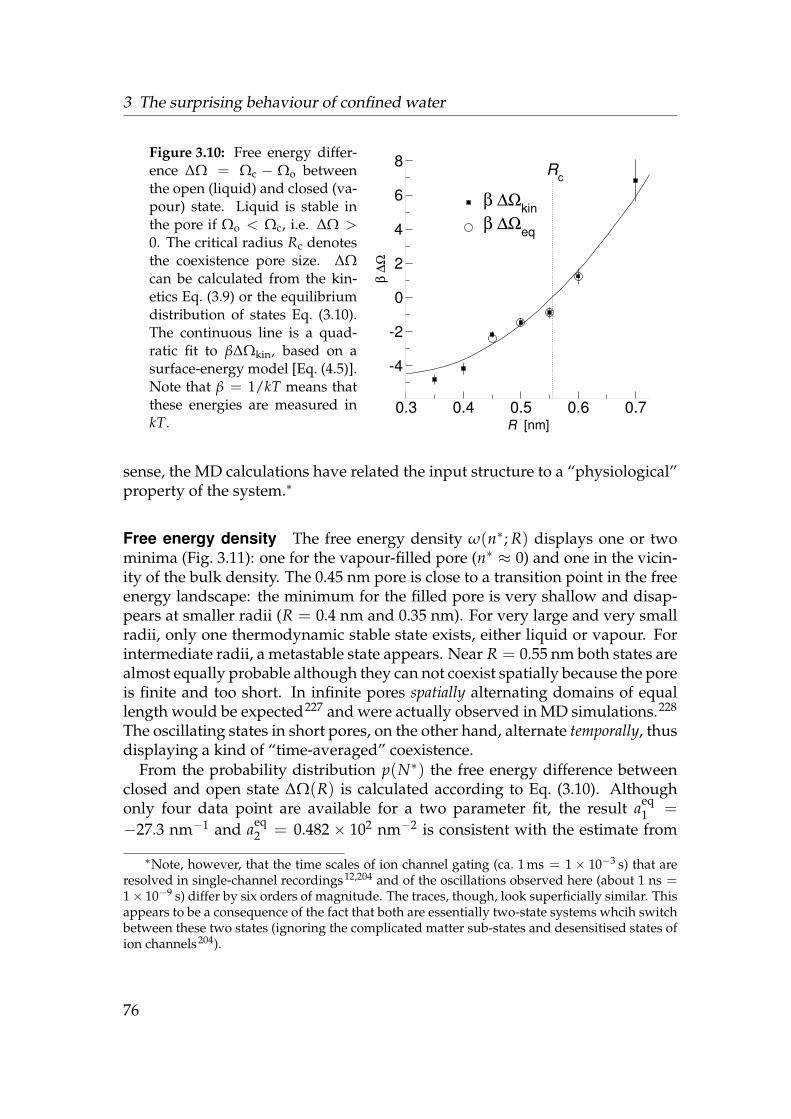
3 The surprising behaviour of confined water
Figure 3.10: Free energy differ-ence ∆Ω = Ωc − Ωo betweenthe open (liquid) and closed (va-pour) state. Liquid is stable inthe pore if Ωo < Ωc, i.e. ∆Ω >0. The critical radius Rc denotesthe coexistence pore size. ∆Ωcan be calculated from the kin-etics Eq. (3.9) or the equilibriumdistribution of states Eq. (3.10).The continuous line is a quad-ratic fit to β∆Ωkin, based on asurface-energy model [Eq. (4.5)].Note that β = 1/kT means thatthese energies are measured inkT.
0.3 0.4 0.5 0.6 0.7R [nm]
-4
-2
0
2
4
6
8
β ∆Ω
β ∆Ωkinβ ∆Ωeq
Rc
sense, the MD calculations have related the input structure to a “physiological”property of the system.∗
Free energy density The free energy density ω(n∗; R) displays one or twominima (Fig. 3.11): one for the vapour-filled pore (n∗ ≈ 0) and one in the vicin-ity of the bulk density. The 0.45 nm pore is close to a transition point in the freeenergy landscape: the minimum for the filled pore is very shallow and disap-pears at smaller radii (R = 0.4 nm and 0.35 nm). For very large and very smallradii, only one thermodynamic stable state exists, either liquid or vapour. Forintermediate radii, a metastable state appears. Near R = 0.55 nm both states arealmost equally probable although they can not coexist spatially because the poreis finite and too short. In infinite pores spatially alternating domains of equallength would be expected227 and were actually observed in MD simulations.228
The oscillating states in short pores, on the other hand, alternate temporally, thusdisplaying a kind of “time-averaged” coexistence.
From the probability distribution p(N∗) the free energy difference betweenclosed and open state ∆Ω(R) is calculated according to Eq. (3.10). Althoughonly four data point are available for a two parameter fit, the result aeq
1 =
−27.3 nm−1 and aeq2 = 0.482× 10² nm−2 is consistent with the estimate from
∗Note, however, that the time scales of ion channel gating (ca. 1 ms = 1× 10⁻³ s) that areresolved in single-channel recordings12,204 and of the oscillations observed here (about 1 ns =1× 10⁻⁹ s) differ by six orders of magnitude. The traces, though, look superficially similar. Thisappears to be a consequence of the fact that both are essentially two-state systems whcih switchbetween these two states (ignoring the complicated matter sub-states and desensitised states ofion channels204).
76
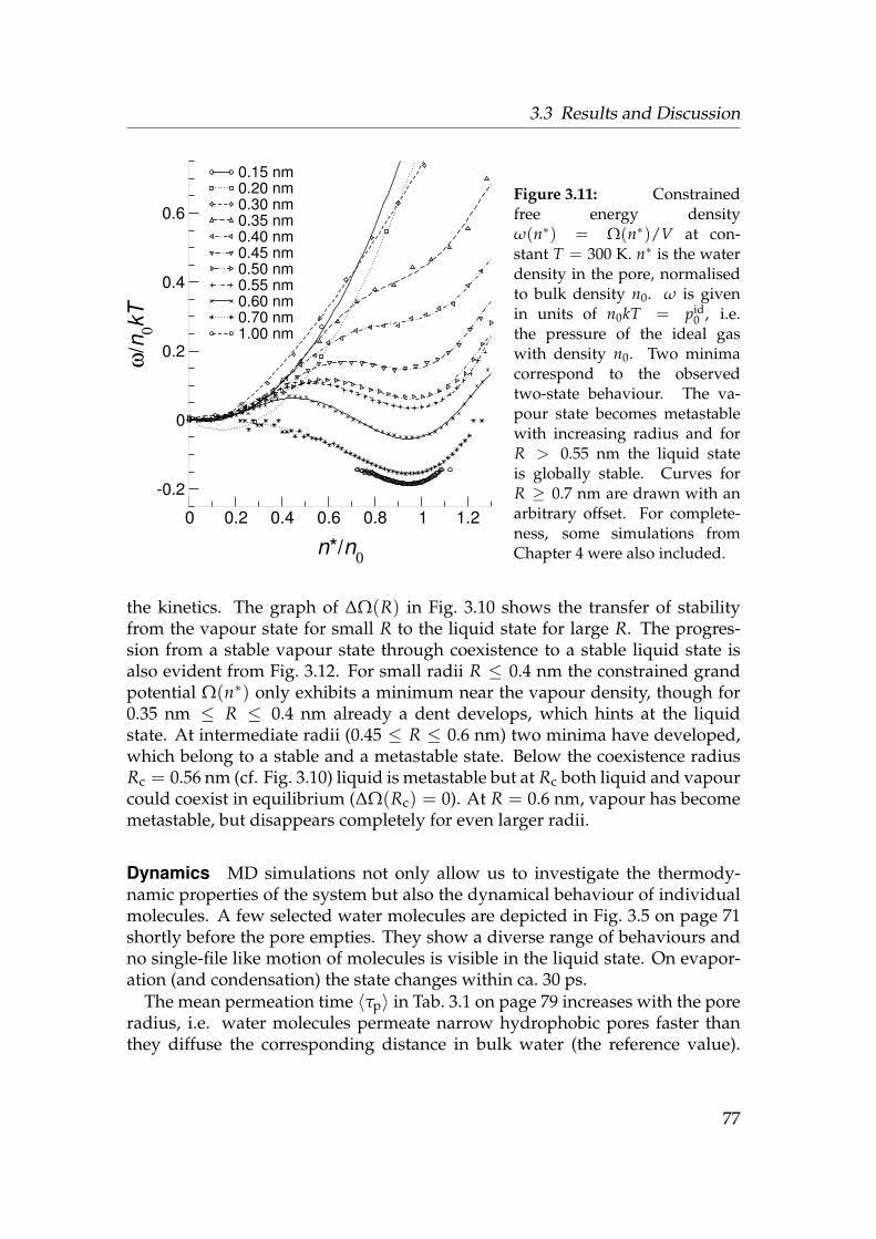
3.3 Results and Discussion
0 0.2 0.4 0.6 0.8 1 1.2
n*/n0
-0.2
0
0.2
0.4
0.6
ω/n
0kT
0.15 nm0.20 nm0.30 nm0.35 nm0.40 nm0.45 nm0.50 nm0.55 nm0.60 nm0.70 nm1.00 nm
Figure 3.11: Constrainedfree energy densityω(n∗) = Ω(n∗)/V at con-stant T = 300 K. n∗ is the waterdensity in the pore, normalisedto bulk density n0. ω is givenin units of n0kT = pid
0 , i.e.the pressure of the ideal gaswith density n0. Two minimacorrespond to the observedtwo-state behaviour. The va-pour state becomes metastablewith increasing radius and forR > 0.55 nm the liquid stateis globally stable. Curves forR ≥ 0.7 nm are drawn with anarbitrary offset. For complete-ness, some simulations fromChapter 4 were also included.
the kinetics. The graph of ∆Ω(R) in Fig. 3.10 shows the transfer of stabilityfrom the vapour state for small R to the liquid state for large R. The progres-sion from a stable vapour state through coexistence to a stable liquid state isalso evident from Fig. 3.12. For small radii R ≤ 0.4 nm the constrained grandpotential Ω(n∗) only exhibits a minimum near the vapour density, though for0.35 nm ≤ R ≤ 0.4 nm already a dent develops, which hints at the liquidstate. At intermediate radii (0.45 ≤ R ≤ 0.6 nm) two minima have developed,which belong to a stable and a metastable state. Below the coexistence radiusRc = 0.56 nm (cf. Fig. 3.10) liquid is metastable but at Rc both liquid and vapourcould coexist in equilibrium (∆Ω(Rc) = 0). At R = 0.6 nm, vapour has becomemetastable, but disappears completely for even larger radii.
Dynamics MD simulations not only allow us to investigate the thermody-namic properties of the system but also the dynamical behaviour of individualmolecules. A few selected water molecules are depicted in Fig. 3.5 on page 71shortly before the pore empties. They show a diverse range of behaviours andno single-file like motion of molecules is visible in the liquid state. On evapor-ation (and condensation) the state changes within ca. 30 ps.
The mean permeation time 〈τp〉 in Tab. 3.1 on page 79 increases with the poreradius, i.e. water molecules permeate narrow hydrophobic pores faster thanthey diffuse the corresponding distance in bulk water (the reference value).
77

3 The surprising behaviour of confined water
0 0.5 1
0
5
10
0.15 nm0.20 nm0.30 nm
0 0.5 1
0
5
10
0.35 nm0.40 nm
0 0.5 1
n*/n0
-5
0
5
10βΩ
0.45 nm0.50 nm0.55 nm0.60 nm
0 0.5 1
-15
-10
-5
0
0.70 nm1.00 nm
Figure 3.12: Constrained grand potential Ω(n∗) of water in hydrophobic pores. Thefree energy βΩ is displayed (in units of kT) over the water density n∗ in the pore. Thegraphs are grouped according to the stability of the liquid or vapour state. n0 is thebulk density of SPC water at 300 K and 1 bar. The same simulations as in Fig. 3.11 areshown. All curves are arbitrarily shifted to coincide in the vapour state.It is no coincidence that the data always span about 10 kT. It is a consequence ofthe length of the equilibrium simulations. The largest free energy difference that canbe estimated from a trajectory of length T, when frames of length ∆t were saved, is∆Wmax = −kT ln ∆t/T. For T = 100 ns and ∆t = 2× 10⁻³ ns, ∆Wmax = 10.8 kT, whichis the maximum ∆Ω in the data presented here. The minimum ∆t that can be useful isthe correlation time of the system,110 or rather, of the property of interest. Typical timescales in the water/pore systems: water reorientation time τ ≈ 1 ps, change of state(filling/emptying) ca. 30 ps; for the density fluctuations in the pore the correlation timehas not been measured. Data points based on a single frame are not reliable, and thesepoints tend to be rather noisy, so they were excluded from the polynomial fits of Ω(n∗)and ω(n∗).
78
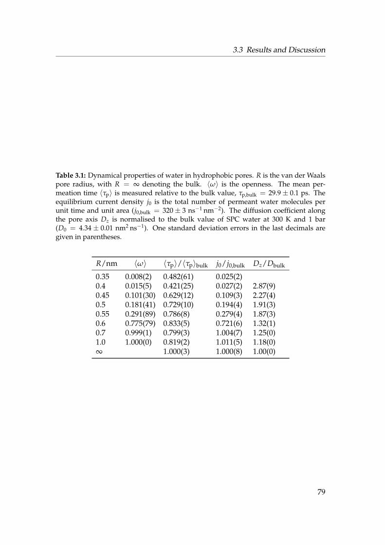
3.3 Results and Discussion
Table 3.1: Dynamical properties of water in hydrophobic pores. R is the van der Waalspore radius, with R = ∞ denoting the bulk. 〈ω〉 is the openness. The mean per-meation time 〈τp〉 is measured relative to the bulk value, τp,bulk = 29.9± 0.1 ps. Theequilibrium current density j0 is the total number of permeant water molecules perunit time and unit area (j0,bulk = 320± 3 ns−1 nm−2). The diffusion coefficient alongthe pore axis Dz is normalised to the bulk value of SPC water at 300 K and 1 bar(D0 = 4.34 ± 0.01 nm2 ns−1). One standard deviation errors in the last decimals aregiven in parentheses.
R/nm 〈ω〉 〈τp〉/〈τp〉bulk j0/j0,bulk Dz/Dbulk
0.35 0.008(2) 0.482(61) 0.025(2)0.4 0.015(5) 0.421(25) 0.027(2) 2.87(9)0.45 0.101(30) 0.629(12) 0.109(3) 2.27(4)0.5 0.181(41) 0.729(10) 0.194(4) 1.91(3)0.55 0.291(89) 0.786(8) 0.279(4) 1.87(3)0.6 0.775(79) 0.833(5) 0.721(6) 1.32(1)0.7 0.999(1) 0.799(3) 1.004(7) 1.25(0)1.0 1.000(0) 0.819(2) 1.011(5) 1.18(0)∞ 1.000(3) 1.000(8) 1.00(0)
79

3 The surprising behaviour of confined water
This is consistent with higher diffusion coefficients Dz in the narrow pores (upto almost three times the bulk value). The diffusion coefficient perpendicularto the pore axis, Dxy, drops to approximately half the bulk value. Martı andGordillo229 also observe increased diffusion in simulations on water in carbonnanotubes (Dz ≤ 1.65 D0) and a corresponding decrease in Dxy. Experimentalstudies on water transport through desformyl gA190 can be interpreted in termsof a Dz of five times the bulk value. Histograms for τp show that there is a con-siderable population of ‘fast’ water molecules (e.g. the black and the blue onein Fig. 3.5 on page 71 with τp between 2 and 10 ps, which is not present in bulkwater. The acceleration of water molecules in the pore can be understood as aneffect of 1D confinement. The random 3D motion is directed along the pore axisand the particle advances in this direction preferentially because there is onlyvery weak attraction between particle and wall. The effect increases with de-creasing radius, i.e. increasing confinement. The average equilibrium currentdensity j0 follows the trend of the openness closely but more detailed time-resolved analysis shows water translocation to occur in bursts in all pores. Innarrow pores, bursts occurring during the “closed” state contribute up to 77%of the total flux. For single-file pores, simulations191,197 and theory230 also pointtowards collective motions of a number of water molecules as the predominantform of transport.
Capillary condensation The behaviour as described so far bears the hall-marks of capillary condensation and evaporation194,207,231 although it is mostoften associated with physical systems which are macroscopically extended inat least one dimension such as slits or long pores. Capillary condensation canbe discussed in terms of the Kelvin equation,193
lnpp0
= −βγlvvlr
, (3.20)
which describes how vapour at pressure p relative to its bulk-saturated pres-sure p0 coexists in equilibrium with its liquid. Liquid and vapour are dividedby an interfacial meniscus of curvature 1/r (r > 0 if the surface is convex); γlvis the surface tension between liquid and vapour and vl the molecular volumeof the liquid. Although the Kelvin equation is not expected to be quantitative insystems of dimensions of only a few molecular diameters it is still useful for ob-taining a qualitative picture. Curvature 1/r and contact angle θ in a cylindricalpore of radius R are related by R = r cos θ. With the Young equation,
γwv = γwl + γlv cos θ, (3.21)
Eq. (3.20) becomes
lnp(R)
p0= −β(γwv − γwl)vl
R, (3.22)
80

3.3 Results and Discussion
Ref. p f × 1014 Φ0[cm3s−1] [ns−1]
Aqp1 187 4.9 3.2Aqp4 187 15 9.7AqpZ 188 2.0 1.3gAa 189 1.6 1.0desformyl gAb 190 110 71
R = 0.35 nm 4.0 2.6R = 0.40 nm 5.7 3.7R = 0.45 nm 30.0 19.4R = 0.50 nm 66.5 43.0R = 0.55 nm 117 75.8R = 0.60 nm 363 235R = 0.70 nm 700 453R = 1.0 nm 1480 956carbon nanotubec 197 26.2 16.9desformyl gA (DH)d 191 10 5.8
abacterial peptide channel gramicidin Abdesformylated gramicidin Ac(6, 6) carbon nanotube, R ≈ 0.24 nmddesformyl gA in the double-helical conformation
Table 3.2: Osmotic permeabil-ity coefficient p f and equilib-rium flux Φ0 of water in se-lected simulations and experi-ments. We used the relationshipp f = 1
2 Φ0vl from Ref. 191 in or-der to compare non-equilibriumexperiments (upper half of thetable) with equilibrium molecu-lar dynamics simulations (lowerhalf). vl = 3.09 × 10⁻²³ cm3 isthe volume of a water moleculein the liquid state.
independent of the interface. For our system, the surface tension between liquidwater and the wall, γwl > 0, and between vapour and the wall, γwv > 0, arefixed quantities. The hydrophobicity of the wall implies γwv < γwl, i.e. the wallis preferentially in contact with vapour; vl can be considered constant. Hence,for a given pore of radius R there exists one vapour pressure p(R) > p0 atwhich vapour and liquid can exist in equilibrium. Water only condenses in thepore if the actual vapour pressure exceeds p(R). Otherwise, only vapour willexist in the pore. The effect is strongest for very narrow pores. Hence a higherpressure is required to overcome the surface contributions, which stabilize thevapour phase in narrow pores. The pressure fluctuates locally in the liquidbulk “reservoir.” These fluctuations can provide an increase in pressure abovethe saturation pressure in the pore and thus drive oscillations between vapourand liquid.
Comparison with experiments, simulations, and a theoretical model Ex-periments on aquaporins187,188 and gA189,190 yield osmotic permeability coef-ficients of water, p f , of the order of 10−12 to 10−14 cm3s−1. We calculate
81
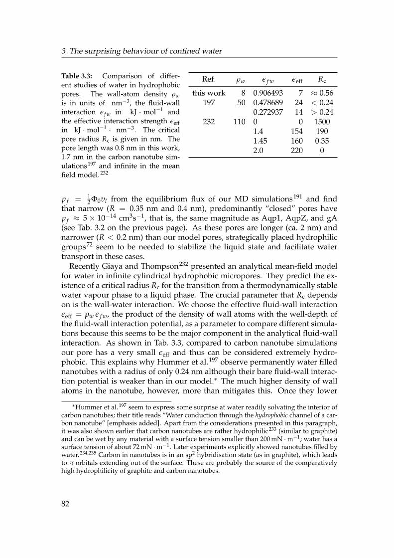
3 The surprising behaviour of confined water
Table 3.3: Comparison of differ-ent studies of water in hydrophobicpores. The wall-atom density ρwis in units of nm−3, the fluid-wallinteraction ε f w in kJ · mol−1 andthe effective interaction strength εeffin kJ · mol−1 · nm−3. The criticalpore radius Rc is given in nm. Thepore length was 0.8 nm in this work,1.7 nm in the carbon nanotube sim-ulations197 and infinite in the meanfield model.232
Ref. ρw ε f w εeff Rc
this work 8 0.906493 7 ≈ 0.56197 50 0.478689 24 < 0.24
0.272937 14 > 0.24232 110 0 0 1500
1.4 154 1901.45 160 0.352.0 220 0
p f = 12 Φ0vl from the equilibrium flux of our MD simulations191 and find
that narrow (R = 0.35 nm and 0.4 nm), predominantly “closed” pores havep f ≈ 5× 10⁻¹⁴ cm3s−1, that is, the same magnitude as Aqp1, AqpZ, and gA(see Tab. 3.2 on the previous page). As these pores are longer (ca. 2 nm) andnarrower (R < 0.2 nm) than our model pores, strategically placed hydrophilicgroups72 seem to be needed to stabilize the liquid state and facilitate watertransport in these cases.
Recently Giaya and Thompson232 presented an analytical mean-field modelfor water in infinite cylindrical hydrophobic micropores. They predict the ex-istence of a critical radius Rc for the transition from a thermodynamically stablewater vapour phase to a liquid phase. The crucial parameter that Rc dependson is the wall-water interaction. We choose the effective fluid-wall interactionεeff = ρw ε f w, the product of the density of wall atoms with the well-depth ofthe fluid-wall interaction potential, as a parameter to compare different simula-tions because this seems to be the major component in the analytical fluid-wallinteraction. As shown in Tab. 3.3, compared to carbon nanotube simulationsour pore has a very small εeff and thus can be considered extremely hydro-phobic. This explains why Hummer et al.197 observe permanently water fillednanotubes with a radius of only 0.24 nm although their bare fluid-wall interac-tion potential is weaker than in our model.∗ The much higher density of wallatoms in the nanotube, however, more than mitigates this. Once they lower
∗Hummer et al.197 seem to express some surprise at water readily solvating the interior ofcarbon nanotubes; their title reads “Water conduction through the hydrophobic channel of a car-bon nanotube” [emphasis added]. Apart from the considerations presented in this paragraph,it was also shown earlier that carbon nanotubes are rather hydrophilic233 (similar to graphite)and can be wet by any material with a surface tension smaller than 200 mN ·m−1; water has asurface tension of about 72 mN ·m−1. Later experiments explicitly showed nanotubes filled bywater.234,235 Carbon in nanotubes is in an sp2 hybridisation state (as in graphite), which leadsto π orbitals extending out of the surface. These are probably the source of the comparativelyhigh hydrophilicity of graphite and carbon nanotubes.
82
3.4 Conclusions
their εeff to double of our value, they also observe strong evaporation. This sug-gests that the close packing of wall atoms within a nanotube may result in be-haviour not seen in biological pores. The mean field model agrees qualitativelywith the simulations as it also shows a sharp transition and high sensitivity toεeff.
The force field employed here and in Ref. 197 did not include polarisationeffects. In the light of the preceding discussion one might anticipate that ad-ditional attractive interactions from the polarizability of the pore wall shouldhave an influence on the liquid-vapour equilibrium. This is the case, as Hansenand coworkers showed in simulations of water in model pores which includeda polarizable pore wall.198,236 Although the effect on structural properties of theconfined water is small, there is a marked shift in the critical radius with increas-ing dielectric constant of the wall. The net-effect of polarizable walls appears tobe an increase in the effective wall-water interaction.
3.4 Conclusions
We have described oscillations between vapour and liquid states in short (LP =0.8 nm), hydrophobic pores of varying radius (0.35 nm≤ R ≤ 1.0 nm). Qual-itatively, this behaviour is explained as capillary evaporation, driven by pres-sure/density fluctuations in the water “reservoir” outside the pore. Similarbehaviour is found in simulations by different authors with different watermodels [SPC (this work), SPC/E,198,202,236 TIP3P (data not shown), TIP3P,197
TIP4P199] in different nanopores [atomistic flexible models (this work), carbonnanotubes,197 spherical cavities,1 and smooth cylinders198,199,202].
We presented a radically simplified model for a nanopore that is perhapsmore hydrophobic than real proteins (although we note the existence of a hy-drophobic pore in the MscS channel55 which has been shown to exhibit dewet-ting in recent MD simulations56). From comparison with experimental data onpermeability we conclude that strategically placed hydrophilic groups are es-sential for the functioning of protein pores. The comparatively high permeabil-ity of our “closed” pores suggests pulsed water transport as one possible mech-anism in biological water pores. Local hydrophobic environments in pores maypromote pulsatory collective transport and hence rapid water and solute trans-location.
Our results indicate new, intrinsically collective dynamic behaviour not seenon simulation time scales currently considered sufficient in biophysical simu-lations. These phase oscillations in simple pores—a manifestation of the hy-drophobic effect—require more than 50 ns of trajectory data to yield a coherentpicture over a free energy range of 10 kT. We thus cannot safely assume thatthe behaviour of water within complex biological pores may be determined by
83

3 The surprising behaviour of confined water
extrapolation from our knowledge of the bulk state or short simulations alone.
84
4 Hydrophobic gating
A hydrophobic constriction site is thought to act as an efficientbarrier to ion and water permeation if its diameter is less thanthe diameter of an ion’s first hydration shell (hydrophobic gating).Simplified pore models allow the investigation of the primarycharacteristics of a conduction pathway, namely its geometry, thechemical character of the pore wall surface, and its local flexibilityand surface roughness. Extended molecular dynamic simulationsshow that a short hydrophobic pore is closed to water for radiismaller than 0.45 nm. By increasing the polarity of the pore wall(and thus reducing its hydrophobicity) closed pores can be openeduntil for hydrophilic pores liquid water is stable even in single-file pores. Ions behave similarly but the transition from conduct-ing to non-conducting pores is even steeper and occurs at a radiusof 0.65 nm for hydrophobic pores. The presence of water vapourin a constriction zone indicates a barrier for ion permeation. Athermodynamic model can explain the behaviour of water in nan-opores in terms of the surface tensions, which leads to a simplemeasure of hydrophobicity—the classical contact angle. Increasedlocal flexibility decreases the permeability of polar species and sodoes an increase in temperature. Both effects can be explained bya decrease in the effective solvent-surface attraction which in turnleads to an increase in the solvent-wall surface tension.
4.1 Geometry, surface character, and localflexibility
Based on a number of atomic resolution structures of ion chan-nels16,27–29,48,51,55,237 and aquaporins69–71,238 an atomistic understanding ofthe transport and gating properties of these proteins is emerging. If we viewtransport proteins as molecular machines which are designed by evolutionto perform selective and efficient transport that can be controlled, i.e. gated,then we can ask what the “building blocks” of these machines are. Thisinvolves not only identification and structural characterisation of the proteindomains involved in gating, but also, at a more abstract level, understanding
85

4 Hydrophobic gating
the underlying physical principles.Here we address the questions of what are physical properties that are im-
portant for the permeation of ions and water, and what is their effect? In partic-ular we will focus on how the flow of ions and water can be controlled, i.e. wewill investigate possible gating mechanisms. This interest is based on the ob-servation that the putative gate in many known ion channel structures (in par-ticular, the nicotinic acetylcholine receptor nAChR,29 the bacterial potassiumchannels KcsA16 and KirBac1.1,48 and the mechanosensitive channels MscL51
and MscS55) is formed by a constriction made from hydrophobic residues. Forexample, the closed state nAChR structure displays an ion pathway which isstill wide enough (radius R ≈ 0.31 nm) to admit three water molecules (radiusof a water molecule rw = 0.14 nm) or one potassium ion (rK+ = 0.133 nm) withhalf of its first hydration shell intact. It is somewhat surprising that a pore doesnot have to be completely physically occluded to prevent the flow of ions. Onthe other hand ions can readily move through the KcsA16,27 selectivity filter al-though its radius is less than 0.15 nm. When an ion enters the filter it has to shedits hydration shell at a high cost in free energy—the solvation free energy for apotassium ion is about−320 kJ ·mol−1 (Ref. 239). The filter is lined by backboneoxygen atoms which coordinate the potassium ion and substitute for its hydra-tion shell, thus reducing the desolvation barrier of +320 kJ ·mol−1 to about+12 kJ ·mol−1 (Ref. 240, 241). The putative gates differ from the selectivity fil-ter in that they are lined by hydrophobic residues. For nAChR29,65 and MscL51,66
it was already hypothesised that these residues cannot substitute for water mol-ecules so that the energetic cost of desolvation prevents the passage of the ion.Though not specifically in the context of gating, Brownian dynamics simula-tions (BD), carried out by Chung et al.64, showed that ions would not traversea non-polar R = 0.4 nm pore unless the polarity of the pore wall was enhancedby embedding dipoles. The authors acknowledged the problem of representingwater as a continuum in the constriction site in BD, which supports the use offully atomistic molecular dynamics simulations in the following.
It appears that the geometry of a pore (its radius, length and shape) and thechemical character of the pore wall have a great influence on the permeation of ionsand water. In addition, local flexibility (i.e. fluctuations in the protein structureas opposed to concerted larger scale motions) of the pore lining might play arole, as seen in simulations of K+ permeation through KcsA.240
It seems difficult to comprehend the dynamical nature of transport phenom-ena from static crystal structures alone. Computational methods can be usedto complement the experimentally observed picture. In particular, classicalmolecular dynamics (MD) can be used to investigate the behaviour of wateror ionic solutions in the environment presented by a protein. This realisticenvironment, however, makes it difficult to disentangle the contributions of
86
4.2 Methods and Theory
various pore properties. In order to reduce the number of parameters sim-plified pore models can be designed to capture the characteristics in ques-tion.62,96,195,196,198,202,242 We focus on the influence of geometry, pore wall char-acter and flexibility. In the last chapter we investigated the behaviour of waterin these “nanopores”. In particular, we found that below a critical radius liquidwater becomes unstable in the pore and the pore is predominantly filled withwater vapour.96 We hypothesised that a pore environment which cannot sustainliquid water would also present a high energetic barrier to an ion.62 Althoughit seems plausible that absence of water would imply the absence of ions it hasnot been demonstrated previously.
Here we explicitly consider ions in model pores and explore dimensions, porewall character, and flexibility in more detail than in the last chapter. We alsopresent a simple thermodynamic model based on surface energies that explainsthe observed behaviour of water in hydrophobic pores.
4.2 Methods and Theory
First, the setup of the model system and the parameters of the MD simulationsare discussed. Then the state based analysis, that was already used implicitlyin the last chapter, is formally introduced. Finally, a simple thermodynamicmodel for liquid-vapour equilibrium in cylindrical pores, based on surface ten-sion arguments, is presented. It is applied in the Results section to explain thesimulation data.
4.2.1 Model
The pore models were constructed as described Section 3.2.1. Briefly, they con-sist of concentric rings of methane-like pseudo-atoms of van der Waals radius0.195 nm (Fig. 4.1 on the next page). These are held in their equilibrium positionby harmonic restraints with spring constant k0 = 1000 kJ ·mol−1 · nm−2. A poreconsists of two mouth regions (length 0.4 nm, i.e. one layer of pseudo-atoms,and radius 1.0 nm) at either end of the constriction site of length L (variedbetween 0.4 nm and 2.0 nm) and radius R (varied between 0.15 nm and 1.0 nm).The pore was embedded in a membrane mimetic, a slab of pseudo-atoms heldon a cubic lattice with unit cell length 0.39 nm with harmonic springs of strengthk0. Pores with a polar surface were created by placing partial charges of ±0.38eon atomic sites 0.2 nm apart. The resulting dipole moments pointed parallel tothe pore axis with a magnitude of 3.6 D each, which is comparable to the dipolemoment of the peptide bond (ca. 3.7 D, Ref. 243).
87

4 Hydrophobic gating
Figure 4.1: Simulation system: Thesolvent-accessible surface of a modelpore with pore radius R = 0.55 nmis shown in light blue (parts of thepore close to the observer are removedfor clarity). The pore is not com-pletely hydrophobic due to two di-poles (red/blue) in the pore wall whichhave the same magnitude as the pep-tide bond dipole. Water molecules inthe pore are depicted in licorice repres-entation and as lines in the mouth re-gion or the bulk (image created withvmd43 and Raster3D44).
4.2.2 Molecular Dynamics
MD simulations were performed with gromacs version 3.1.4 (Ref. 127) andthe SPC water model.132 Parameters for the unified methane atoms and ionsare described in Section 2.2.3 on page 38. The integration time step was 2 fsand coordinates were saved every 2 ps. With periodic boundary conditions,long range electrostatic interactions were computed with a particle mesh Ewaldmethod (real space cutoff 1 nm, grid spacing 0.15 nm, 4th order interpola-tion164,165) while the short range van der Waals forces were calculated withina radius of 1 nm. The neighbour list (radius 1 nm) was updated every 10 steps.Weak coupling algorithms166 were used to simulate at constant temperature(T = 300 K, time constant 0.1 ps) and pressure (P = 1 bar, compressibility4.5× 10−5 bar−1, time constant 1 ps) with the x and y dimensions of the simu-lation cell held fixed at 4 nm. The total thickness of the water reservoir in thez-direction was 3.0 nm, ensuring bulk-like water behaviour far from the mem-brane mimetic. The initial system configuration was created by solvating theslab-embedded pore model with water. For simulations with ions, some watermolecules were replaced with ions to reach the target concentration. Initiallythere were always ions present in pores with R ≥ 0.4 nm. A typical simulationbox measured 3.9× 3.9× 4.6 nm3 and contained about 1500 water moleculesand 280 pseudo-atoms (and between 25 to 28 Na+ and Cl− ions each).
88

4.2 Methods and Theory
4.2.3 State based analysis
We define discrete states by mapping equilibrium states of the whole system(snapshots from the MD equilibrium trajectory) onto numbers ωi. The sameapproach is used in statistical mechanics to map different microscopic statesto one macroscopic state, characterised by the value of a state variable, herecalled ω. This approach is used to label the two phase states that the pore waterexhibits in our simulations. We either find liquid-filled pores or vapour-filledones. Due to the small pore volumes “vapour” typically refers to zero or onewater molecule in the cavity. We use the density in the pore as an indicatorof the phase state. We assign the state using a Schmitt-trigger procedure204 inorder to avoid spurious state changes due to fluctuations from the interfacial re-gion. When the water density n(t) rises above 0.65 of the density of bulk watern0 = 1.0 g · cm−1 (at T = 300 K and P = 1 bar) the liquid state, i.e. ω = 1, isassigned to the phase state at time t. When n(t) drops below 0.25 n0 the vapourstate (ω = 0) is assigned. The pore in the liquid-filled state is termed “open”because our simulations show that significant amounts of water pass throughit; furthermore, we also demonstrate in this work that a pore that sustains a li-quid environment potentially allows ions to permeate. A vapour-plugged pore,however, will prevent ion permeation and is said to be “closed”.
Liquid-filled pores and vapour-filled pores are assumed to be in equilibrium.The “openness” or probability for the occurrence of the liquid, i.e. open, state is
〈ω〉 = 1T
∫ T
0dt ω(t) =
To
T, (4.1)
where T denotes the total simulation time, To the total time that the pore isopen, whereas Tc is the total time in the vapour or closed state. If 〈ω〉 > 1
2 thenequilibrium is on the side of liquid (and vapour is a meta stable state), otherwisethe stable phase state is vapour. The equilibrium is governed by the equilibriumconstant
K(R) =Tc(R)To(R)
=T− To(R)To(R)
= 〈ω(R)〉−1 − 1, (4.2)
which is trivially related to the openness. (Note that for To = 0 or Tc = 0 it ismeaningless to compute K because it indicates that the simulation time was tooshort to sample any state changes.)
4.2.4 Model for liquid-vapour equilibrium in pores
We investigate a subsystem of the whole simulation system comprising of thepore of volume V = LπR2. The subsystem can exchange water molecules withthe bulk water outside the pore, which acts as a particle reservoir at average
89

4 Hydrophobic gating
chemical potential µ. µ is implicitly determined by the constant average dens-ity of water in the bulk system, which in turn is prescribed by simulating atconstant pressure. Hence we can use the grand potential Ω(T, V, µ) = −pV asthe free energy to describe the subsystem in the closed and open state.202 Theequilibrium constant K is determined by the free energy difference between theclosed (vapour) and open (liquid) state,
β ∆Ω(R) = β [Ωv(R)−Ωl(R)] = − ln K(R) = − ln(〈ω(R)〉−1 − 1
). (4.3)
Following Evans207, we write the free energy difference between the vapourand the liquid state with the corresponding surface contributions as
∆Ω(R) = Ωv(R)−Ωl(R) =
− pv(T, µ) L πR2 + 2πR L γvw + 2πR2γlv −(−pl(T, µ)L πR2 + 2πR L γlw
).
(4.4)
Here the index w indicates the solid pore wall, l the liquid and v the vapourphase; for instance γlv is the surface tension or surface free energy per unitarea of the liquid-vapour interface. The system is fairly close to bulk phasecoexistence so we can expand the pressure p around the saturation chemicalpotential µsat(T) in a Taylor series
p(T, µ) = p(T, µsat) + (µ− µsat)∂p(T, µ)
∂µ
∣∣∣∣µ=µsat
+ · · · ,
where at saturation pl(T, µsat) = pv(T, µsat). This leads to a simple parabolicform for the free energy difference between the two states:
∆Ω(R) =[2γlv −
(µ− µsat
)(nv(T, µsat)− nl(T, µsat)
)L]πR2 + 2πL(γvw − γlw)R
= 2[γlv +
12
∆µ ∆nvl L]π R2 + 2πL ∆γw R, (4.5)
where we define the distance of the state from saturation ∆µ := µ − µsat, thedifference in densities ∆nvl := nl− nv at saturation, and the difference in surfacefree energies of the two phases with the wall, ∆γw := γvw − γlw. The term∆µ∆nvl L is small for L < 10 nm as the system is close to phase coexistence (forL ≈ 1 nm it is about 10−3 times smaller than γlv = 17 kT nm−2 when estimatedfrom ∆nvl ∆µ L ≈ ∆P L ≈ 1 bar× L = 2.4× 10⁻² kT nm−3 × L, T = 300 K)and will be neglected. Only the difference between the surface free energiesenters the model so we express it as the contact angle θe, using the macroscopic
90
4.3 Results and Discussion
definition from the Young equation γvw − γlw = γlv cos θe (see, for instance,Ref. 92). Then Eq. (4.5) becomes
∆Ω(R, L, θe) = 2π R γlv(R + L cos θe). (4.6)
(Eq. (4.6) is similar to the simple model derived by Allen et al.202 but it includesγvw − γlw and hence θe instead of just γlw.) For fixed pore length L and a givenpore material, characterised by θe, the graph of ∆Ω(R) over the pore radius Rdescribes a parabola containing the origin. Although it is not a priori obviousthat such a macroscopic treatment (Eq. (4.5) or Eq. (4.6)) of a nanoscale systemis meaningful, the MD results for the free energy difference presented in Sec-tion 4.3.1 can be adequately explained within this model.
The connection between the model free energy ∆Ω(R) and the behaviour ofthe system as observed in MD simulations, i.e. the openness 〈ω(R)〉, is estab-lished by inverting Eq. (4.3), yielding
〈ω(R)〉 = 11 + exp[−β ∆Ω(R)]
. (4.7)
For linear ∆Ω(R) this represents a sigmoidal curve but non-linear terms (as inEq. (4.5)) change its shape considerably.
4.3 Results and Discussion
First we investigate the behaviour of pure water in nanopores and quantifythe influence of geometry, pore surface, and local flexibility on the equilibriumbetween liquid and vapour filled pores. Then simulations for a NaCl electrolyteare analysed and compared to the pure water case. The intention behind thesestudies is to explore more fully the ways in which a hydrophobic gate maybe opened, and how other factors might modulate such hydrophobic gating.This is particularly important in the context of current models for the gating ofnAChR29,59 that suggest that the transition between the closed and open statesof the pore involves both an increase in pore radius and in polarity. We also notethat recent discussion of the state (open vs. closed) of MscS have suggested ahydrophobic gating mechanism,56 similar to that proposed for nAChR.62
4.3.1 Pure water
A large number of simulations were run for water in model pores (total simula-tion time > 5 µs) in order to investigate the influence of pore radius (0.15 nm ≤R ≤ 1 nm) and pore surface character (hydrophobic vs. amphipathic vs. hy-drophilic). Local flexibility (wall atom positional root mean square deviations
91
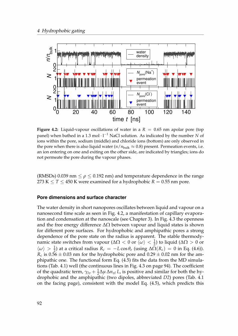
4 Hydrophobic gating
0
1n/
n bulk
waterdensity
0
1
2
N
Npore(Na+)
permeationevent
0 20 40 60 80 100 120 140time t [ns]
01
2
N
Npore(Cl-)
permeationevent
Figure 4.2: Liquid-vapour oscillations of water in a R = 0.65 nm apolar pore (toppanel) when bathed in a 1.3 mol · l−1 NaCl solution. As indicated by the number N ofions within the pore, sodium (middle) and chloride ions (bottom) are only observed inthe pore when there is also liquid water (n/nbulk ≈ 0.8) present. Permeation events, i.e.an ion entering on one and exiting on the other side, are indicated by triangles; ions donot permeate the pore during the vapour phases.
(RMSDs) 0.039 nm ≤ ρ ≤ 0.192 nm) and temperature dependence in the range273 K ≤ T ≤ 450 K were examined for a hydrophobic R = 0.55 nm pore.
Pore dimensions and surface character
The water density in short nanopores oscillates between liquid and vapour on ananosecond time scale as seen in Fig. 4.2, a manifestation of capillary evapora-tion and condensation at the nanoscale (see Chapter 3). In Fig. 4.3 the opennessand the free energy difference ∆Ω between vapour and liquid states is shownfor different pore surfaces. For hydrophobic and amphipathic pores a strongdependence of the pore state on the radius is apparent. The stable thermody-namic state switches from vapour (∆Ω < 0 or 〈ω〉 < 1
2 ) to liquid (∆Ω > 0 or〈ω〉 > 1
2 ) at a critical radius Rc = −L cos θe (using ∆Ω(Rc) = 0 in Eq. (4.6)).Rc is 0.56± 0.03 nm for the hydrophobic pore and 0.29± 0.02 nm for the am-phipathic one. The functional form Eq. (4.5) fits the data from the MD simula-tions (Tab. 4.1) well (the continuous lines in Fig. 4.3 on page 94). The coefficientof the quadratic term, γlv +
12 ∆µ ∆nvl L, is positive and similar for both the hy-
drophobic and the amphipathic (two dipoles, abbreviated D2) pores (Tab. 4.1on the facing page), consistent with the model Eq. (4.5), which predicts this
92

4.3 Results and Discussion
Table 4.1: Parameters of the thermodynamic model Eq. (4.5) fitted to the MD results andresulting contact angle θe. Experimental values for γlv = 72× 10−3 Jm−2 = 17 kT nm−2
and θe ≈ 118 for water on a flat methyl (–CH3) terminated self assembled mono-layer244,245 indicate that the simple thermodynamic model gives the right order of mag-nitude results. (All values at room temperature.)
pore surface character γlv +12 ∆µ ∆nvl L ∆γw = γvw − γlw θe
[kT nm−2] [kT nm−2] []
bare CH4 0 “hydrophobic” +10±1 −7.2±0.2 134±3two dipoles D2 “amphipathic” +8.2±0.5 −3.0±0.2 111±2four dipoles D4 “hydrophilic” +2.8±0.5 +1.8±0.2 51±10
coefficient to be independent of the pore wall. For the polar pore (four dipoles,D4) the data are more ambiguous. Only if the first two data points at smallradii are excluded from the fit as outliers is this coefficient positive (but stillthree times smaller than the one for the less hydrophilic pores). The outliersshow that a high density of local charges leads to a higher probability of thepore being liquid-filled than predicted by the macroscopic model, possibly in-dicating a shortcoming of the model to subsume inhomogeneous potentials intothe surface tension terms. For our system parameters, the coefficient is in factdominated by the water liquid-vapour surface tension γlv (see Section 4.2.4 onpage 89) and hence we will use its value as an approximation to γlv. ∆γw, thedifference in surface tensions between the wall and vapour or liquid, becomesmore positive with increasing polarity of the pore wall. It effectively measuresthe hydrophobicity of the wall. This becomes even more apparent when the(macroscopic) contact angle cos θe = ∆γw/γlv is formally computed (Tab. 4.1).Macroscopically, a hydrophobic surface can be defined as one with θe > 90.This allows us to call the apolar pore (θe = 134) “hydrophobic” compared tothe “amphipathic” pore D2 (θe = 111; still hydrophobic but with some “hydro-philic” patches). A “hydrophilic” pore like the D4 system (θe ≈ 51) is charac-terised by ∆γw > 0 or θe < 90 and liquid is always the preferred phase in thepore, regardless of R.
Experimental macroscopic contact angles θe for water on flat methyl (–CH3)terminated self assembled monolayers are reported up to 118.244,245 A “mi-croscopic contact angle” of 135 ± 15 was calculated for a droplet of 90 watermolecules (radius R ≈ 0.75 nm) on a methyl terminated film from MD simula-tions,246 consistent with our result of θe = 134. MD simulations seem to over-estimate the experimental equilibrium contact angle. In this context we notethat although the macroscopic equilibrium contact angle is only establishedabout 10 nm from the contact line, the local contact angle θl in the core struc-
93
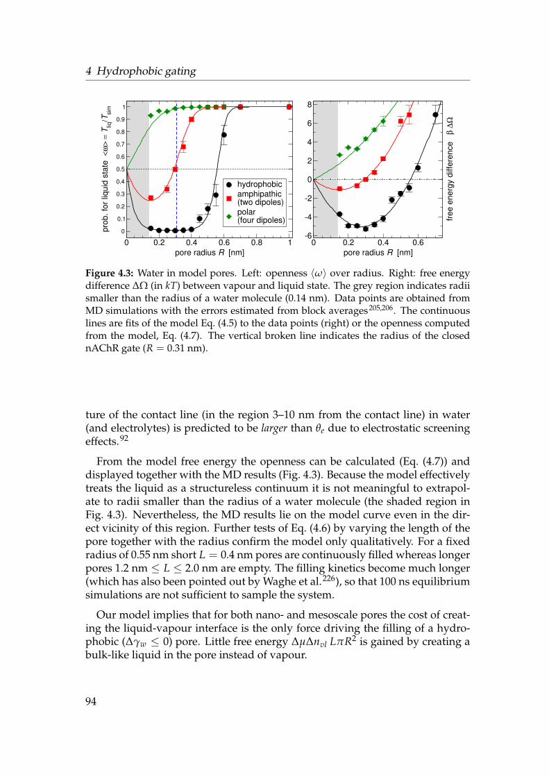
4 Hydrophobic gating
0 0.2 0.4 0.6 0.8 1pore radius R [nm]
0
0.1
0.2
0.3
0.4
0.5
0.6
0.7
0.8
0.9
1pr
ob. f
or li
quid
sta
te <
ω>
= T liq
/Tsi
m
hydrophobicamphipathic(two dipoles)polar(four dipoles)
0 0.2 0.4 0.6pore radius R [nm]
-6
-4
-2
0
2
4
6
8
free
ener
gy d
iffer
ence
β
∆Ω
Figure 4.3: Water in model pores. Left: openness 〈ω〉 over radius. Right: free energydifference ∆Ω (in kT) between vapour and liquid state. The grey region indicates radiismaller than the radius of a water molecule (0.14 nm). Data points are obtained fromMD simulations with the errors estimated from block averages205,206. The continuouslines are fits of the model Eq. (4.5) to the data points (right) or the openness computedfrom the model, Eq. (4.7). The vertical broken line indicates the radius of the closednAChR gate (R = 0.31 nm).
ture of the contact line (in the region 3–10 nm from the contact line) in water(and electrolytes) is predicted to be larger than θe due to electrostatic screeningeffects.92
From the model free energy the openness can be calculated (Eq. (4.7)) anddisplayed together with the MD results (Fig. 4.3). Because the model effectivelytreats the liquid as a structureless continuum it is not meaningful to extrapol-ate to radii smaller than the radius of a water molecule (the shaded region inFig. 4.3). Nevertheless, the MD results lie on the model curve even in the dir-ect vicinity of this region. Further tests of Eq. (4.6) by varying the length of thepore together with the radius confirm the model only qualitatively. For a fixedradius of 0.55 nm short L = 0.4 nm pores are continuously filled whereas longerpores 1.2 nm ≤ L ≤ 2.0 nm are empty. The filling kinetics become much longer(which has also been pointed out by Waghe et al.226), so that 100 ns equilibriumsimulations are not sufficient to sample the system.
Our model implies that for both nano- and mesoscale pores the cost of creat-ing the liquid-vapour interface is the only force driving the filling of a hydro-phobic (∆γw ≤ 0) pore. Little free energy ∆µ∆nvl LπR2 is gained by creating abulk-like liquid in the pore instead of vapour.
94

4.3 Results and Discussion
0 4 8 12 16 20
k [102 kBT nm-2]
-6
-4
-2
0
2
free
ener
gy d
iffer
ence
β
∆Ω
0.5 1 1.5
ρ(R=0.55nm,k) [10-1 nm]
-6
-4
-2
0
2
β ∆Ω
∆Ω(R=0.55nm,k) [MD]∆Ω(R,k) = ∆Ω(R-∆ρ(k),k0)
0
0.5
1
1.5
2
2.5
RM
SD
ρ [
10-1
nm
]
β ∆Ω(R=0.55nm,k)[MD]ρ(k) [theory: harm.osc. at T=300K]ρ(R=0.55nm, k) [MD]
liquidvapour
(a) (b)
Figure 4.4: Influence of flexibility on the liquid-vapour equilibrium. (a) For a hydro-phobic R = 0.55 nm pore the harmonic restraint force constant k of the pore wall atomswas varied, resulting in a range of RMSDs ρ, which show the expected behaviour ofthermic harmonic oscillators. The free energy difference ∆Ω between liquid and va-pour states of water in the pore shows strong dependence on the local flexibility ρ;rigid pores contain liquid water whereas flexible ones favour vapour. The effect cannot be explained by a reduction of the effective pore radius by ρ alone [broken line in(b)]. All data at T = 300 K.
Local flexibility
The influence of local fluctuations in protein structure can be modelled by chan-ging the harmonic spring constant k that holds the pore wall atoms at theirequilibrium positions. In a simplified picture of a harmonic oscillator with anaverage energy kBT/2 per degree of freedom the RMSD ρ is directly related
to k by ρ(k) =√〈∆rmax〉
2 =√
3kBT/k. This simple model overestimates themeasured RMSDs by only 10–20% (Tab. 4.2 on the next page), showing that thewall atoms behave like almost independent, thermally driven, harmonic oscil-lators (Fig. 4.4(a)). At a fixed radius, increasing the flexibility (smaller k, hencegreater ρ) shifts the equilibrium towards vapour (Fig. 4.4). Conversely, a morerigid wall favours the condensation of water in the pore. Thus, water does not“push away” the pore walls to fill the pore but rather fluctuating pore wallsappear to disfavour the formation of adjacent water layers. This effect cannot
95
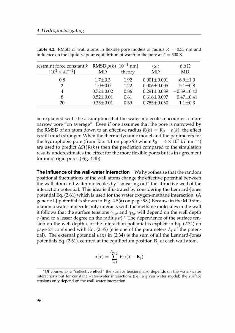
4 Hydrophobic gating
Table 4.2: RMSD of wall atoms in flexible pore models of radius R = 0.55 nm andinfluence on the liquid-vapour equilibrium of water in the pore at T = 300 K.
restraint force constant k RMSD ρ(k) [10−1 nm] 〈ω〉 β ∆Ω[102 × kT−2] MD theory MD MD
0.8 1.7±0.3 1.92 0.001±0.001 −6.9±1.02 1.0±0.0 1.22 0.006±0.005 −5.1±0.84 0.72±0.02 0.86 0.291±0.089 −0.89±0.438 0.52±0.01 0.61 0.616±0.097 0.47±0.41
20 0.35±0.01 0.39 0.755±0.060 1.1±0.3
be explained with the assumption that the water molecules encounter a morenarrow pore “on average”. Even if one assumes that the pore is narrowed bythe RMSD of an atom down to an effective radius R(k) = R0 − ρ(k), the effectis still much stronger. When the thermodynamic model and the parameters forthe hydrophobic pore (from Tab. 4.1 on page 93 where k0 = 4× 10² kT nm−2)are used to predict ∆Ω
(R(k)
)then the prediction compared to the simulation
results underestimates the effect for the more flexible pores but is in agreementfor more rigid pores (Fig. 4.4b).
The influence of the wall-water interaction We hypothesise that the randompositional fluctuations of the wall atoms change the effective potential betweenthe wall atom and water molecules by “smearing out” the attractive well of theinteraction potential. This idea is illustrated by considering the Lennard-Jonespotential Eq. (2.61) which is used for the water oxygen-methane interaction. (Ageneric LJ potential is shown in Fig. 4.5(a) on page 98.) Because in the MD sim-ulation a water molecule only interacts with the methane molecules in the wallit follows that the surface tensions γvw and γlw will depend on the well depthε (and to a lesser degree on the radius σ).∗ The dependence of the surface ten-sion on the well depth ε of the interaction potential is explicit in Eq. (2.34) onpage 24 combined with Eq. (2.35) (ε is one of the parameters λi of the poten-tial). The external potential u(x) in (2.34) is the sum of all the Lennard-Jonespotentials Eq. (2.61), centred at the equilibrium position Rj of each wall atom.
u(x) =Nwall
∑j=1
VLJ(x− Rj)
∗Of course, as a “collective effect” the surface tensions also depends on the water-waterinteractions but for constant water-water interactions (i.e. a given water model) the surfacetensions only depend on the wall-water interaction.
96

4.3 Results and Discussion
In order to appreciate the influence of flexibility or temperature we discuss acoarse grained version of the LJ potential. This is necessary because in Sec-tion 2.1.2 (in particular Eq. (2.15) and (2.19)) the wall was treated as an externalfield and hence the movement of the wall atoms was not accounted for. Wewant to derive a version of (2.61) which incorporates “on average” the effect offluctuations in the wall, i.e. fluctuations in the positions of the wall atoms. Wenotice that for a rigid (or “frozen”) wall the probability to find an atom near itsequilibrium position x′ is
p(x; x′) = δ(x− x′),
i.e. it will only be found at x′. For a harmonicly bound atom at finite temperat-ure T > 0 (or β < ∞) the spatial probability is Gaussian distributed as
p(x; x′, β) = g(x− x′, β) =1
(2π)3/2ρ(β)exp
[−1
2
(|x− x′|
ρ(β)
)2]
where the Gaussian g has a half width equal to the RMSD ρ(β). This leads tothe coarse grained potential
VLJ(x, β) = g ? VLJ =∫
d3x′ g(x− x′, β)VLJ(x′). (4.8)
Unfortunately, (4.8) diverges due to the divergence at the LJ centre. To overcomethis problem we argue that the influence of flexibility is more strongly felt inthe slowly varying, attractive component of the LJ potential. Following Weeks,Chandler, and Anderson123 we decompose VLJ in attractive and repulsive parts(Fig. 4.5(b)),
VLJ(x) = Vrep(x) + Vattr(x), with (4.9)
Vrep(x) :=
VLJ(x) + ε if |x| < 21/6σ
0 if |x| ≥ 21/6σ(4.10)
Vattr(x) :=
−ε if |x| < 21/6σ
VLJ(x) if |x| ≥ 21/6σ(4.11)
where the centre of the potential is taken to be at x = 0. Applying the thermalbroadening to the attractive component Vattr yields
Vattr(x, β) = g(x, β) ? Vattr(x) =∫
d3x′ g(x− x′, β)VLJ(x′), (4.12)
which is shown for the 1D case in Fig. 4.5(c). Finally, the coarse grained LJpotential is taken as the sum
VLJ(x, β) = Vrep(x) + Vattr(x, β). (4.13)
97
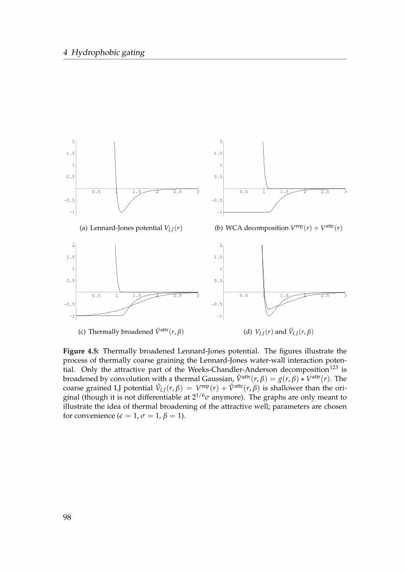
4 Hydrophobic gating
0.5 1 1.5 2 2.5 3
-1
-0.5
0.5
1
1.5
2
(a) Lennard-Jones potential VLJ(r)
0.5 1 1.5 2 2.5 3
-1
-0.5
0.5
1
1.5
2
(b) WCA decomposition Vrep(r) + Vattr(r)
0.5 1 1.5 2 2.5 3
-1
-0.5
0.5
1
1.5
2
(c) Thermally broadened Vattr(r, β)
0.5 1 1.5 2 2.5 3
-1
-0.5
0.5
1
1.5
2
(d) VLJ(r) and VLJ(r, β)
Figure 4.5: Thermally broadened Lennard-Jones potential. The figures illustrate theprocess of thermally coarse graining the Lennard-Jones water-wall interaction poten-tial. Only the attractive part of the Weeks-Chandler-Anderson decomposition123 isbroadened by convolution with a thermal Gaussian, Vattr(r, β) = g(r, β) ? Vattr(r). Thecoarse grained LJ potential VLJ(r, β) = Vrep(r) + Vattr(r, β) is shallower than the ori-ginal (though it is not differentiable at 21/6σ anymore). The graphs are only meant toillustrate the idea of thermal broadening of the attractive well; parameters are chosenfor convenience (ε = 1, σ = 1, β = 1).
98
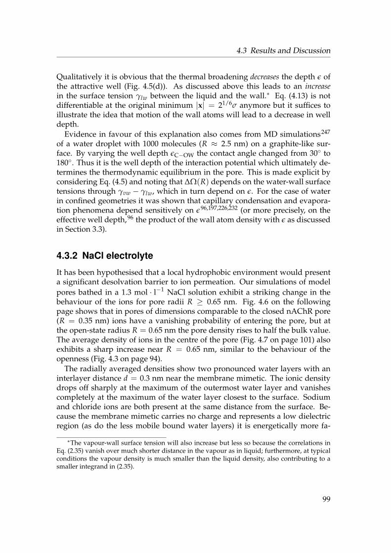
4.3 Results and Discussion
Qualitatively it is obvious that the thermal broadening decreases the depth ε ofthe attractive well (Fig. 4.5(d)). As discussed above this leads to an increasein the surface tension γlw between the liquid and the wall.∗ Eq. (4.13) is notdifferentiable at the original minimum |x| = 21/6σ anymore but it suffices toillustrate the idea that motion of the wall atoms will lead to a decrease in welldepth.
Evidence in favour of this explanation also comes from MD simulations247
of a water droplet with 1000 molecules (R ≈ 2.5 nm) on a graphite-like sur-face. By varying the well depth εC−OW the contact angle changed from 30 to180. Thus it is the well depth of the interaction potential which ultimately de-termines the thermodynamic equilibrium in the pore. This is made explicit byconsidering Eq. (4.5) and noting that ∆Ω(R) depends on the water-wall surfacetensions through γvw − γlw, which in turn depend on ε. For the case of waterin confined geometries it was shown that capillary condensation and evapora-tion phenomena depend sensitively on ε96,197,226,232 (or more precisely, on theeffective well depth,96 the product of the wall atom density with ε as discussedin Section 3.3).
4.3.2 NaCl electrolyte
It has been hypothesised that a local hydrophobic environment would presenta significant desolvation barrier to ion permeation. Our simulations of modelpores bathed in a 1.3 mol · l−1 NaCl solution exhibit a striking change in thebehaviour of the ions for pore radii R ≥ 0.65 nm. Fig. 4.6 on the followingpage shows that in pores of dimensions comparable to the closed nAChR pore(R = 0.35 nm) ions have a vanishing probability of entering the pore, but atthe open-state radius R = 0.65 nm the pore density rises to half the bulk value.The average density of ions in the centre of the pore (Fig. 4.7 on page 101) alsoexhibits a sharp increase near R = 0.65 nm, similar to the behaviour of theopenness (Fig. 4.3 on page 94).
The radially averaged densities show two pronounced water layers with aninterlayer distance d = 0.3 nm near the membrane mimetic. The ionic densitydrops off sharply at the maximum of the outermost water layer and vanishescompletely at the maximum of the water layer closest to the surface. Sodiumand chloride ions are both present at the same distance from the surface. Be-cause the membrane mimetic carries no charge and represents a low dielectricregion (as do the less mobile bound water layers) it is energetically more fa-
∗The vapour-wall surface tension will also increase but less so because the correlations inEq. (2.35) vanish over much shorter distance in the vapour as in liquid; furthermore, at typicalconditions the vapour density is much smaller than the liquid density, also contributing to asmaller integrand in (2.35).
99

4 Hydrophobic gating
R 0.35 nm 0.6 nm 0.65 nm 0.75 nm
wat
erN
a+C
l−
densityscale:water: nbulkions: mol l−1
0.05
0.10
0.20
0.30
0.40
0.50
0.60
0.70
0.80
0.90
1.00
1.10
1.20
1.30
1.40
Figure 4.6: Equilibrium densities of water (top row), sodium ions (middle) and chlorideions (bottom) in hydrophobic model pores of radii R = 0.35 nm to 0.75 nm; the NaClbulk concentration is 1.3 mol · l−1. The narrow 0.35 nm pore mimics the closed gateof nAChR whereas the wide 0.65 nm pore approximates the open channel. Althoughwide enough to admit the ions physically, the narrow pore is effectively closed to ions(“hydrophobic gating”). The membrane mimetic is located in the horizontal regionwhich appears black, i.e. void of water, in all images.
100

4.3 Results and Discussion
0.2 0.4 0.6 0.8 1R [nm]
0
0.2
0.4
0.6
0.8
1
pore
cor
e de
nsity
n/
n bulk Na+
Cl-
water (NaCl)water only
Figure 4.7: Ionic density in the core regionof hydrophobic pores. The core is takento have a radius of about one ionic radius(0.1 nm) and exhibits the highest density ofions. The core density increases markedlyat the critical radius R = 0.65 nm. The coredensity follows the openness (as shown forwater in Fig. 4.3). The dip in density atR = 0.7 nm is due to very few state changesin the 150 ns simulation and a subsequentbias towards a 70 ns vapour period; in gen-eral the state switching frequency in theelectrolyte systems is reduced compared tothe pure water case (see also Fig. 4.2). Bulkconcentration of ions is 1.3 mol · l−1. Linesare drawn as guides to the eye.
vourable for the ions to be solvated in the high dielectric region of the bulk-likewater. The bound water layers are not a consequence of the presence of the ionsas they also form in pure water near a hydrophobic surface with the same in-terlayer spacing of 0.3 nm (see Fig. 3.3 on page 69 and Fig. 3.4), and in this caseeven a third water layer is discernible with d = 0.35 nm. Water ordering in cyl-indrical and slit pores in the absence of ions was also observed in simulationsby other groups.195,196,202,210,213,248 Effectively, ions are excluded from a zone ofthickness 0.6 nm (Na+) or 0.7 nm (Cl−) from the surface. The ion exclusion layerstretches into the pore without interruption so that at R = 0.65 nm there is onlya narrow channel of easily displaceable water which can admit ions. For widerpores, the ion density in the pore approaches bulk values (Fig. 4.7).
Although the absence of ionic density can be taken as a strong indication fora closed pore, the presence of equilibrium density does not necessarily implya functionally open state, as the latter also requires rapid permeation of ionsthrough a pore. As MD simulations output the trajectories of water and ions,the equilibrium flux (Φ0), i.e. the total number of particles per nanosecondwhich completely permeate the pore, can be measured. Fig. 4.8 on the nextpage shows Φ0 for ions and water molecules (both for water in a 1.3 mol · l−1
NaCl electrolyte and for pure water) in hydrophobic pores of varying radius ona logarithmic scale. Water flux is about three orders of magnitude larger thanion flux and increases rapidly with increasing radii as long as R is smaller thanthe critical radius Rc = 0.62 nm. Beyond Rc (when liquid becomes the stablephase) the slope in the logarithmic plot decreases from 15 nm−1 to 2.4 nm−1.The water current density Φ0/(πR2) reaches a constant value of 300 ns−1 nm−2
so the increase for R > Rc is only due to the increase in pore diameter. The
101
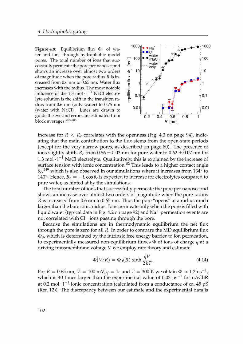
4 Hydrophobic gating
Figure 4.8: Equilibrium flux Φ0 of wa-ter and ions through hydrophobic modelpores. The total number of ions that suc-cessfully permeate the pore per nanosecondshows an increase over almost two ordersof magnitude when the pore radius R is in-creased from 0.6 nm to 0.65 nm. Water fluxincreases with the radius. The most notableinfluence of the 1.3 mol · l−1 NaCl electro-lyte solution is the shift in the transition ra-dius from 0.6 nm (only water) to 0.75 nm(water with NaCl). Lines are drawn toguide the eye and errors are estimated fromblock averages.205,206
0.2 0.4 0.6 0.8 1R [nm]
0.01 0.01
0.1 0.1
1 1
10 10
100 100
1000 1000
equi
libriu
m fl
ux Φ
0 [ns
-1]
Na+
Cl-
water(NaCl)wateronly
increase for R < Rc correlates with the openness (Fig. 4.3 on page 94), indic-ating that the main contribution to the flux stems from the open-state periods(except for the very narrow pores, as described on page 80). The presence ofions slightly shifts Rc from 0.56± 0.03 nm for pure water to 0.62± 0.07 nm for1.3 mol · l−1 NaCl electrolyte. Qualitatively, this is explained by the increase ofsurface tension with ionic concentration.82 This leads to a higher contact angleθe,249 which is also observed in our simulations where it increases from 134 to140. Hence, Rc = −L cos θe is expected to increase for electrolytes compared topure water, as hinted at by the simulations.
The total number of ions that successfully permeate the pore per nanosecondshows an increase over almost two orders of magnitude when the pore radiusR is increased from 0.6 nm to 0.65 nm. Thus the pore “opens” at a radius muchlarger than the bare ionic radius. Ions permeate only when the pore is filled withliquid water (typical data in Fig. 4.2 on page 92) and Na+ permeation events arenot correlated with Cl− ions passing through the pore.
Because the simulations are in thermodynamic equilibrium the net fluxthrough the pore is zero for all R. In order to compare the MD equilibrium fluxΦ0, which is determined by the intrinsic free energy barrier to ion permeation,to experimentally measured non-equilibrium fluxes Φ of ions of charge q at adriving transmembrane voltage V we employ rate theory and estimate
Φ(V; R) = Φ0(R) sinhqV
2 kT. (4.14)
For R = 0.65 nm, V = 100 mV, q = 1e and T = 300 K we obtain Φ ≈ 1.2 ns−1,which is 40 times larger than the experimental value of 0.03 ns−1 for nAChRat 0.2 mol · l−1 ionic concentration (calculated from a conductance of ca. 45 pS(Ref. 12)). The discrepancy between our estimate and the experimental data is
102

4.3 Results and Discussion
0 0.2 0.4 0.6 0.8 1 1.2water density mouth and pore nMP/nbulk
0
2
4
6
8
10
12
βΩ(T
,nM
P)
273 K300 K310 K330 K350 K373 K400 K450 K
(a) Change of the free energy land-scape Ω(n, T) with T.
300 350 400 450T [K]
0
0.1
0.2
0.3
0.4
0.5
0.6
open
ness
<ω
>
openness <ω>
-7
-6
-5
-4
-3
-2
-1
0
1
β ∆Ω
β ∆Ω = β(Ωvap−Ωliq)
(b) Openness and free energy differencebetween states ∆Ω.
Figure 4.9: Temperature dependence of the liquid-vapour equilibrium in a hydrophobicR = 0.55 nm pore. In (a) the density is calculated over the pore and the mouth regionswhich act as a buffer of constant chemical potential except for T = 273 K, where themouth region also fills with vapour. Continuous lines are polynomial least square fitsof order 4 (or order 6 for 300 K ≤ T ≤ 330 K), reminiscent of a Landau free energy withthe water density in the pore and mouth region nMP as order parameter. The criticalpoint of SPC water is near T = 373 K.
not unexpected as Eq. (4.14) has only qualitative character. Furthermore, nA-ChR presents a more complex pore lining surface than the model pore, and ifthe difference in bath concentrations and access resistance was taken into ac-count the discrepancy would likely be reduced by an order of magnitude. Nev-ertheless, the estimate demonstrates that the intrinsic barrier to ion permeationis small beyond the critical radius.
4.3.3 Sensing external parameters
In the simplest model of sensing a system exists in an equilibrium with twostates. External stimuli shift the equilibrium which elicits a cellular response.For example, a temperature-sensing channel at normal temperature might bein the closed state. Elevated temperature shifts the equilibrium to the openstate and the influx of ions initiates a signalling cascade that terminates in thesensation of heat. However, the exact mechanisms of gating by temperature ofe.g. TRP channels remain obscure,21 though it is now known that TRP channelsare voltage gated250 and temperature shifts their voltage-dependent activation
103

4 Hydrophobic gating
curves.∗
We tested the influence of temperature in the range from 273 K to 450 K onwater in the R = 0.55 nm hydrophobic pore (data points for T > 373 K represent“supercritical” water because the critical point for the SPC water model is closeto T = 373 K). The free energy landscape of the water-pore system depends onthe temperature (Fig. 4.9(a) on the previous page). With increasing temperaturethe liquid state (i.e. near water bulk density) decreases in stability. Accord-ingly, the openness decreases with temperature so that the vapour state, i.e. theclosed stated, dominates at higher temperatures (Fig. 4.9(b)). The decrease inopenness with increasing T indicates that the difference of the wall surface ten-sions ∆γw must become even more negative, i.e. vapour in contact with the wallis increasingly favoured. The effect would be similar to the one discussed forincreased flexibility of wall atoms as the major effect of temperature would beto smear out the interaction potential between water molecules and wall atoms.This example demonstrates in principle how an external signal, an increase intemperature from T = 300 K to 330 K, decreases the openness, and correspond-ingly the flux of water molecules, by a factor of six. Voltage-dependent TRPchannels are probably not directly gated in this manner. Interestingly, their be-haviour is described by a two-state model where the activation energies for theopen-to-closed and closed-to-open transitions differ very much250—similar toa pore predominantly liquid or vapour filled. Perhaps the precarious stabilityof liquid water in hydrophobic cavities is used as a temperature sensor, e.g. bysolvation and desolvation of voltage sensor domains and the change in dielec-tric properties.
4.4 Conclusions
We have explicitly demonstrated a hydrophobic gating mechanism for ions, us-ing simplified hydrophobic pores as models for the closed gates of ion channels.There is a critical radius Rc above which a pore becomes effectively permeableto water or ions. Rc ≈ 0.56 nm for water and Rc ≈ 0.65 nm for ions, is muchlarger than the radius for a water molecule or a bare ion alone. This correl-ates nicely with the current view that the closed state structures of many ionchannels contain gates formed by hydrophobic constriction sites. In nAChR theradius of the putative gate is 0.31 nm, 0.17 nm in MscL, and 0.13 nm in KcsA.Models of KcsA and of Kv channels in their open states, based on the MthK andKvAP structures respectively, have gate radii of about 0.6 nm (Ref. 251), whereas
∗The voltage dependent activation curves of TRP channels are also shifted by ligands suchas capsaicin (the “hot” ingredient of chilli peppers) or menthol.250 Thus, the sensation of heator cold elicited by some food is the same sensation that is felt when the temperature is increasedor decreased.
104

4.4 Conclusions
the open-state nAChR structure opens up to about 0.65 nm. Our simulationsshow that the polarity of the pore wall can shift the critical radius consider-ably. This is reflected in the proposed gating mechanism of nAChR.59 Not onlydoes the radius of the constriction site increase but hydrophobic sidechains arealso rotated out of the pore to expose the more polar, i.e. hydrophilic, peptidebackbone. By combining hydrophobic gating with a change in surface polar-ity only a moderate change in radius is required to obtain a large physiologicaleffect. Changes in local flexibility may also modulate the gating behaviour. Itis too early to ascertain their importance as such changes in flexibility have notbeen widely investigated experimentally for channels (or any other proteins).There are suggestions of possible regulatory roles of changes in flexibility ine.g. KTN domains,252 and in the modulation of binding of TRAP protein tothe Trp operon mRNA.253 Temperature can also affect gating, in a fashion sim-ilar to local flexibility, but temperature sensitive voltage-dependent TRP chan-nels are most likely not directly gated by temperature in the manner describedhere, though water-solvation of the voltage sensors—and hence their dielectricenvironment—could be temperature dependent.
A thermodynamic model based on surface energies fits remarkably well thedata of the atomic-scale MD simulation, even for very small radii. Though sucha macroscopic treatment is not a priori expected to give a satisfactory descriptionof a microscopic system there are other examples as for instance classical nucle-ation theory, which shares some similarities with our and others’ models94,202.It generally agrees quite well with experiments on the condensation of dropletsfrom vapour, which implies that the use of macroscopic surface tension is valideven for droplets of radii of about 1 nm (Ref. 113). It appears that in this casewater structure (i.e. a hydrogen bond network) is only important insofar thatit is responsible for different wall-fluid surface tensions. Also, Nicholls et al.254
find in their investigations of the interfacial and thermodynamic properties ofhydrocarbons that the “macroscopic concept of interfacial free energy is applic-able at the molecular level.” Our results seem to corroborate the conclusions ofMaibaum and Chandler255 that two-state behaviour of water in pores shouldonly require a cold liquid close to phase coexistence and sufficiently differentvapour-wall and liquid-wall surface tensions (which is, of course, where the“special” properties of water reside in such a model).
We have sketched out principles of gating mechanisms in ion channels, basedon model channels. Ion channels in nature display complex conformational dy-namics in relationship to gating. There is a need for better single molecule meth-ods for ion channels to probe these phenomena experimentally. Combined elec-trical and optical methods look promising in this respect256 although consider-able improvements in time resolution are still required. In the meantime thereis a continued role for simulations and theory to enable us to bridge betweenstatic structure and dynamic function.
105

4 Hydrophobic gating
In addition to hydrophobic gating per se, our studies suggest the possible im-portance of gate flexibility in regulation of biological activity. The relationshipbetween static structures, conformational change, and intrinsic flexibility in re-lationship to proteins and signalling merits further active investigation. In arecent review of protein-protein interactions and conformational changes, Gohet al.257 conclude that there is increasing support for a pre-existing equilibriummodel. In such a model, proteins exist in a population of conformations, withligand binding leading to a change in the probability distribution of the en-semble. Some evidence in support of this have been obtained from recent sim-ulation studies of ligand binding proteins (e.g. Ref. 258) but further (single-molecule) experimental and computational studies of a wider range of proteinsare needed to more firmly establish the general importance of changes in flex-ibility.
106

5 The dielectric barrier and thehydrophobic effect
A hydrophobic pore of sub-nanometre dimensions can appear im-permeable to an ion even though its radius is still much wider thanthe one of the ion. The barrier to ion permeation is quantifiedby calculating the potential of mean force (PMF) from umbrella-sampled molecular dynamics simulations. It is compared tocontinuum-electrostatic Poisson-Boltzmann calculations. The lat-ter fail to describe the ion barrier because they do not account forthe properties of the confined water. The barrier originates fromthe energetic cost to desolvate the ion. Even in wide pores, whichcould accommodate an ion and its hydration shell, a barrier of sev-eral kT remains because the liquid water phase is not stable in thehydrophobic pore. Thus, the properties of the solvent play a cru-cial role in determining permeation properties of ions in confine-ment at the molecular scale. For water, the PMF depends stronglyon the wall flexibility. With increasing pore length the barrier ap-pears to reach a constant value.
5.1 A closer look at ions (and water) inhydrophobic pores
Confinement strongly affects the behaviour of water and ions and canlead to effects which are not anticipated from macroscopic descrip-tions.96,193,194,197,218,234,248,259–261 One example is the exclusion of ions from poresthat have radii much larger than the ionic radius as shown in the last chapter.Pores of molecular dimensions (radius R ≤ 1 nm) can be found, for instance, incarbon nanotubes, zeolites, and ion channel proteins. In this chapter we showthat an electrostatic continuum approach alone does not capture the essentialsof ion permeation through pores in a low dielectric. A more detailed atomisticapproach is required that incorporates both the interaction of the water mole-cules with the ion (the hydration shell) and the water-pore interaction (hydro-phobic effects).
The atomistic molecular dynamics (MD) computer simulations of Chapter 4indicated that short (length L = 0.8 nm) model nanopores with a methyl-
107
5 The dielectric barrier and the hydrophobic effect
terminated surface would not allow the passage of ions below a critical radiusR ≤ 0.6 nm. Different effects must play a role in creating a barrier to ion per-meation: For any charged species there is a purely electrostatic “dielectric bar-rier”63 for transferring an ion from a high dielectric phase like water (ε = 78)through a low dielectric membrane (ε ≈ 2), generally referred to as the Bornenergy.82 An atomistic picture includes the interaction between individual wa-ter molecules and the solute, and the entropic cost of accommodating the solutecavity. The energetic cost for stripping the hydration shell off an ion is the freeenergy of solvation. When ions permeate narrow pores they will have to shedparts of their hydration shell. In the context of ion channel gating, it was hypo-thesised that this would create a barrier to ion permeation.29,59,62,64,66
Does the electrostatic continuum approach alone capture the essentials of ionpermeation through low dielectric pores, as perhaps intuition and analytic mod-els63 suggest? Or is a more detailed atomistic approach required? If so, what isthe magnitude of the effect?
In order to address these questions we calculate the potential of mean force(PMF; see Section 2.3.1 on page 46) of ions and water in the hydrophobic poremodels that were also used in Chapter 3 and 4. The pore radius R was var-ied between 0.15 nm and 1.0 nm. These pores are very hydrophobic with thecharacteristics of a methyl-terminated surface. Hence there are no groups thatcould substitute for water molecules in the ion’s hydration shell. The exclusionof ions (and water) from narrow pores (described in Section 4.3.2 on page 99)is quantified in terms of their free energy permeation barrier ∆G‡, which is themaximum of the equilibrium free energy landscape as described by the one-
(a) R = 0.35 nm (b) R = 1.00 nm
Figure 5.1: Ions in pore models. Na+ ions are depicted as blue spheres of radius0.095 nm, with their first hydration shell shown as translucent spheres of radius0.32 nm. The model pores are represented with their solvent excluded surface (imagescreated with vmd43 and Raster3D44).
108

5.2 Methods
dimensional PMF ∆G(z), i.e. the free energy required to position a particle atsubsequent positions z along the pore axis.
The fully atomistic PMF is compared to continuum electrostatic PMF fromPoisson-Boltzmann calculations. These are similar to the ones presented byWeetman et al.262, who calculate the Born profile in cylindrical (radius R =0.25 nm) and hour-glass shaped pores (minimum R = 0.3 nm).
5.2 Methods
Fully atomistic PMFs ∆G(z) are calculated from classical molecular dynamic(MD) trajectories (Section 2.3). Continuum electrostatic PMFs ∆GB(z) (“Bornprofile”) are obtained as the Born energy by solving the Poisson-Boltzmann (PB)equation (Section 2.4).
5.2.1 Molecular dynamics
MD simulations were performed with gromacs version 3.2.1 (Ref. 127) and theSPC water model.132 Parameters for the unified methane atoms and ions aredescribed in Section 2.2.3 on page 38. Simulations were carried out for at least100 ns. All other parameters were identical to the simulations described in Sec-tion 4.2.2 on page 88.
5.2.2 Potential of mean force
The PMF is related to the equilibrium density n(x) through the density of thereference state in the bulk far from the pore n0 (cf. Eq. (2.95) on page 48),
β∆G(x) = − lnn(x)n0
+ β(G0 − µ0).
The free energy of the reference state G0 is an unknown constant, but the nor-malisation with the excess chemical potential for the insertion of the permeantparticle into the bulk liquid, µ0, ensures that G(z) equals 0 in the bulk.
Alternatively, one can bias the equilibrium distribution of a test ion to theenergetically unfavorable regions using the technique of umbrella sampling172
as described in Section 2.3.2 on page 48. We restrained a Na+ ion orwater molecule with a harmonic potential (U(z) = k/2 (z − zi)
2, k =7693 kJ·mol−1·nm−2) at subsequent equally spaced positions zi along the zaxis of the pore (spacing zi − zi−1 = 0.025 nm). This restricted its move-ment to the xy-plane while still allowing diffusion into adjacent windows.For each window a starting frame from an equilibrium trajectory was selected
109
5 The dielectric barrier and the hydrophobic effect
which had the particle in question (ion or water molecule) close to zi (max-imum initial deviation was 0.3 nm, 80% of initial distances were smaller than0.1 nm). One MD simulation of length 0.6 ns was carried out for each of the101 windows, using the same parameters as above. The positional deviationζ(t) = z(t) − zi of the particle was recorded for every step (2 fs). A correla-tion time
∫dt 〈ζ(t)ζ(0)〉/〈ζ2〉 of typically 0.2 ps indicates that ζ was actually
oversampled by a factor of 0.2 ps/2 fs = 100.The 101 biased distributions of z positions of the test particle (ion or water)
were recombined and unbiased with the Weighted Histogram Analysis Method(WHAM)174,175. The first 0.1 ns of each window run were discarded as equilib-ration time, leaving a total of 0.5 ns per window. A tolerance of 10−5 kT in theself-consistent WHAM procedure lead to converged PMFs.
The PMF in the bulk and mouth region of the pore is obtained from the equi-librium MD trajectories. Umbrella sampled PMFs are only meaningful in re-gions where the diffusing of the particle is limited in the xy-plain, i.e. the poreand mouth region. Final PMF profiles were assembled by manually matchingequilibrium profiles and umbrella sampled profiles in the mouth region whereboth methods are accurate.
For ions in pores with R ≥ 0.6 nm only equilibrium MD is necessary to col-lect the complete PMF; sufficient sampling is achieved in 100 ns. Water PMFscould be obtained from equilibrium MD reliably for all radii except for theR = 0.15 nm pore but for comparison the PMF for a water molecule in theR = 0.55 nm pore was also calculated. The umbrella sampled water PMFs weresymmetrized as they exhibited a small skew of about 1 kT (cf. Section 2.3.3).
5.2.3 Poisson-Boltzmann calculations
Poisson-Boltzmann calculations were carried out with apbs.179 The test Na+
ion was assigned a Born radius of 0.1680 nm (Ref. 181).∗ The radius of an im-plicit solvent molecule was set to 0.14 nm, the approximate radius of a watermolecule. The electrostatic PMF or Born profile was calculated according toEq. (2.115) on page 56,
∆GB(z) = Gelpore+ion(z)− Gel
ion(z)− Gelpore. (2.115)
In order to minimise grid artifacts, Gelion was calculated for every position z of
the ion in the channel so that the ion was at the exact same grid position in the∗The Pauling radius of Na+ is only 0.095 nm (Ref. 12) but as pointed out by Rashin and
Honig181, for electrostatic calculations one needs to consider the radius of the cavity within thesolvent. For cations, the radius of the cavity is better approximated by the covalent radius,which is much larger than the ionic radius. Test calculations with the ionic radius did notreproduce the enthalpy of solvation for Na+; the larger Born radius (including an empirical 7%correction181) was required.
110

5.3 Results and Discussion
calculations for the first two terms. Gelpore ≡ 0 because the pore/slab system is
uncharged.Further parameters were chosen as to be consistent with the MD simulations.
The temperature was 300 K, the ionic strength 1.3 M NaCl. The water dielec-tric constant εw was 63 (the value of the SPC water model146). The dielectricconstant εp of the pore and slab material was set to 1 because in the MD simula-tions the material is modelled as simple van der Waals spheres without partialcharges. These can not screen an electric field and hence are best described byεp = 1; a more realistic value for hydrocarbons would be εp = 2.
In addition to the calculations at a concentration of 1.3 mol · l−1 NaCl we alsoperformed the same calculations at 0 mol · l−1 NaCl and 7 mol · l−1 NaCl. Thebinding energy ∆GB shows negligible sensitivity on to the ionic strength. This issensible because the test ion is the only charge in the system. Two sets of calcu-lations with water dielectric coefficient at different values (63 for the SPC watermodel and 78.5 as the experimental value at 300 K) also indicated negligiblesensitivity thereto. The calculations were sensitive to the grid discretization ne-cessary to solve the Poisson-Boltzmann equation by a finite element scheme.Our tests on grid sizes ranging from 65 to 129 grid points indicated that our res-ults are converged for grids of size 97× 97× 97, using a focusing scheme (finalgrid resolution 0.031 nm) and a smoothed dielectric boundary.
5.3 Results and Discussion
In the following we use the PMF as a quantitative measure for the influence of arange of parameters on the permeation properties of ions and water through hy-drophobic pores. We begin by comparing the continuum picture (obtained fromPoisson-Boltzmann calculations) to the fully atomistic one (based on umbrella-sampled MD). This will elucidate the role of the solvent in the process of ionpermeation. Then we have a closer look at ions in wide pores (R = 1 nm)which, at first sight, should already provide a bulk-like environment, but fail todo so. Finally, for the case of water we look at varying the local flexibility of thewall and the length of the pore, at a fixed radius of R = 0.55 nm.
5.3.1 Continuum vs atomistic picture
First we turn to the continuum picture and consider a Born-type analysis of thebarrier that a sodium ion has to overcome if it is to permeate a low dielectric
111
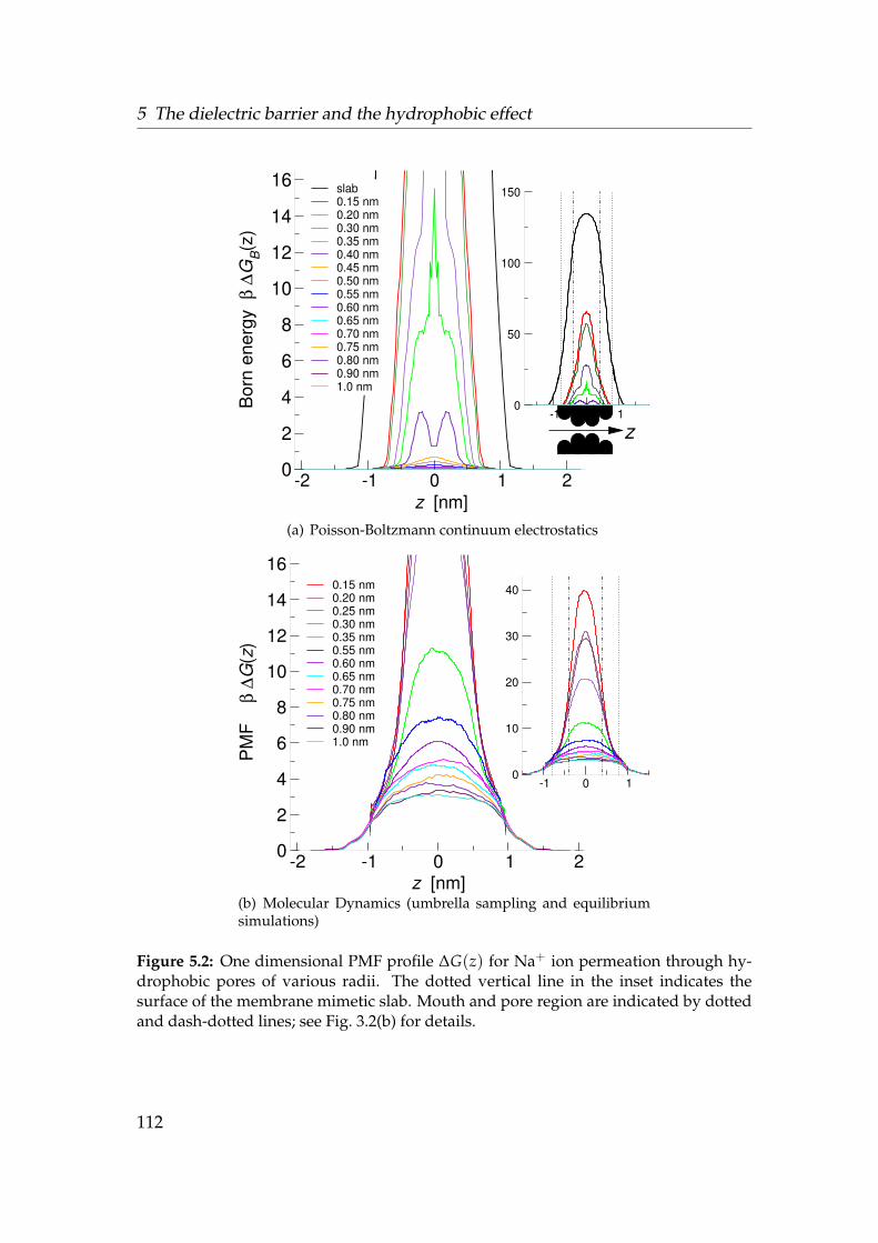
5 The dielectric barrier and the hydrophobic effect
-2 -1 0 1 2z [nm]
0
2
4
6
8
10
12
14
16
Bor
n en
ergy
β ∆
GB(z
)
slab0.15 nm0.20 nm0.30 nm0.35 nm0.40 nm0.45 nm0.50 nm0.55 nm0.60 nm0.65 nm0.70 nm0.75 nm0.80 nm0.90 nm1.0 nm
-1 0 10
50
100
150
z
(a) Poisson-Boltzmann continuum electrostatics
-2 -1 0 1 2z [nm]
0
2
4
6
8
10
12
14
16
PM
F
β ∆G
(z)
0.15 nm0.20 nm0.25 nm0.30 nm0.35 nm0.55 nm0.60 nm0.65 nm0.70 nm0.75 nm0.80 nm0.90 nm1.0 nm
-1 0 10
10
20
30
40
(b) Molecular Dynamics (umbrella sampling and equilibriumsimulations)
Figure 5.2: One dimensional PMF profile ∆G(z) for Na+ ion permeation through hy-drophobic pores of various radii. The dotted vertical line in the inset indicates thesurface of the membrane mimetic slab. Mouth and pore region are indicated by dottedand dash-dotted lines; see Fig. 3.2(b) for details.
112

5.3 Results and Discussion
(εs) slab of thickness l. According to Parsegian63 the Born barrier ∆GB is
β∆GB =β
4πε0
(e2
2εsa− e2
εslln
2εw
εs + εw
)≈ lB
2εsa
(1− 2a
lln 2)
, if εs εw.
(5.1)
a denotes the Born radius of the ion (a = 0.1680 nm for Na+), εw the dielectricconstant of the solvent (water), and lB = βe2/4πε0 the Bjerrum length (lB =56.0 nm at T = 300 K). For ε = 1 and thickness l = 1.6 nm Eq. (5.1) yields∆GB = 142 kT (351 kJ ·mol−1 at T = 300 K, almost the hydration energy 413 kJ ·mol−1 of the sodium ion181). The explicit PB calculation gives a similar barrierof 135 kT [Fig. 5.2(a) on the preceding page]. This demonstrates that even a thinmembrane creates a practically insurmountable barrier to ion permeation.
For a pore with R = 0.55 nm the continuum electrostatic calculations yield∆G‡
B = 0.23 kT, i.e the barrier effectively vanishes. Fig. 5.2(a) shows electrostaticPMFs for pores of various radii R. Only for R ≤ 0.4 nm is the Born barrierappreciable. For R > 0.4 nm it drops below 1 kT (Fig. 5.3 on the followingpage), ceasing to be a barrier for all practical purposes. This is in stark contrastto the results from the atomistic MD simulations [Fig. 5.2(b) on the precedingpage]. For the wide R = 0.55 nm pore an ion still has to overcome a barrier of7.4 kT, and even a pore with a diameter of 2 nm (more than the total thicknessof the slab) will have an appreciable effect on ion permeation (∆G‡ = 3.2 kT).
The failure of the continuum model to describe the PMF in very narrow poresis not unexpected and has been noted before.263,264 It is somewhat more surpris-ing in the wider pores (about R ≥ 0.6 nm) where a continuum description ofthe solvent electrolyte should become feasible. Investigation of the ionic dens-ity in the pore nevertheless shows a 0.6 nm depletion layer near the surface anda density in the wide pore barely reaching 70% of the bulk value (Fig. 5.5(b)on page 116). The strong disagreement between the electrostatic PMF and theatomistic one leads us to look for an explanation for the barrier which is notbased on electrostatics.
The atomistic simulations include by their very nature entropic and shortrange interaction effects in addition to long range electrostatics, and they alsoaccount for the granularity of the solvent, thus admitting density effects. Thesituation in the narrow pores R ≤ 0.3 nm can be interpreted in both picturesin a qualitatively similar way. The pore is too narrow to accommodate solventtogether with the ion. In the Born picture this corresponds to an ion completelyimmersed in a low dielectric environment; in the atomistic picture it is related tothe loss of the hydration shell (perhaps apart from two water molecules in axialpositions—which can still contribute up to half of the total solvation energy170).In both cases it translates into a high energetic barrier. For R ≥ 0.4 nm the ionis enveloped by a shell of high dielectric solvent of thicker than 0.1 nm. This is
113

5 The dielectric barrier and the hydrophobic effect
Figure 5.3: Comparisonof the barrier height ∆G‡
from the electrostatic∆GB(z) and atomistic∆G(z) PMF profiles. Datapoints indicated by filledcircles or diamonds werecalculated from umbrellasampled MD trajector-ies whereas the emptyvariants were directlyobtained from equilib-rium MD. Empty squareswere obtained fromcontinuum-electrostaticPoisson-Boltzmanncalculations.
0.2 0.4 0.6 0.8 1R [nm]
0
10
20
30
40
barr
ier h
eigh
t β
∆G
+ +
Na+ (Poisson-Boltzmann)Na+ (Molecular dynamics)H2O (Molecular Dynamics)
0 0.2 0.4 0.6 0.8 1
10-3
10-2
10-1
100
101
102
103
already enough to lower the Born energy considerably. The continuum calcu-lations assume that the solvent simply exists in the pore. There is no energeticcost associated with filling the pore with water. The PMF for water (Fig. 5.4 onthe next page) shows that the free energy to place a water molecule at the centreof the pore is considerable (between 3 kT and 7 kT for medium sized pores, alsosee Fig. 5.3). This means it is difficult to maintain a solvent environment in thepore which in turn could successfully hydrate and stabilize the ion (althoughcollective effects will reduce the barrier to filling the pore with water somewhatas hinted at in Chapter 3). Hence the reason for the high barrier for ions is notso much the electrostatic contribution of placing a charged particle at the centreof a aqueous pore through a low dielectric membrane but the inability of waterto wet (or solvate) the pore itself.
5.3.2 Ions in wide pores
It seems surprising that ions are considerably affected even in a pore of 2 nmdiameter, greater than its length of 1.6 nm, and about ten times the ionic ra-dius. The radially averaged density from the MD simulations shows that wateralready behaves rather bulk-like in the pore (Fig. 5.5(a) on page 116). It fillsalmost the whole pore volume at bulk density. Near the pore surface the samecharacteristic water layers are visible that are also seen at the slab-reservoir in-terface. The ionic density, Fig. 5.5(b) on page 116, is concentrated in the centralregion and only reaches about 0.9 mol · l−1, i.e. 70% of the bulk value. This ef-fect is not due to insufficient sampling time as investigation of the density plots
114

5.3 Results and Discussion
-2 -1 0 1 2z [nm]
0
2
4
6
8
10
12P
MF
∆G
(z)
[kT]
0.15 nm(umbrella)0.15 nm0.20 nm0.30 nm0.35 nm0.40 nm0.45 nm0.50 nm0.55 nm(umbrella)0.55 nm0.60 nm0.70 nm1.0 nm
Figure 5.4: PMF profilefor water. The PMFwas derived from equilib-rium simulations exceptfor the R = 0.15 nm and0.55 nm pore, where um-brella sampling was em-ployed (heavy lines). Forthese two radii, the equi-librium trajectory derivedPMF is also shown forcomparison (thin lines).
from shorter stretches of the 100 ns trajectory indicates. (About 20 ns appear tobe the minimum time necessary to obtain meaningful densities.)
The effect of the surface on the ions extends noticeably for at least 1 nm. Thisis also borne out by the radial distribution function g(r; Na+, Ow) (Fig. 5.6 onpage 117) from a homogeneous electrolyte (99 ns MD at 1 mol · l−1 NaCl con-centration in a 4× 4× 4 nm3 simulation box, T = 300 K, P = 1 bar). The firstwater peak of height 7.59 is at a distance of 0.226 nm from the Na+ centre butthe second peak is still noticeable (1.44) at 0.447 nm. The first hydration shell ofNa+ contains ca. 4.6 water molecules in a radius of 0.32 nm, while the secondshell adds another 15.6 within 0.53 nm (the number of water molecules N(r)within a sphere of radius r at the minimum following a peak in g(r); see the in-set of Fig. 5.6 on page 117). Thus about 20 water molecules in a sphere of radius0.53 nm are noticeably influenced by a Na+ ion. On the other hand, water layer-ing effects near the hydrophobic surface extend over two to three layers of water(Chapter 3 and 4), influencing water 0.6 nm afar from the surface. Combiningthese two ranges we estimate that the solvent-mediated wall-ion interaction canextend to about 1 nm. Thus ions will still be affected by the pore surface evenif the pore is ten times as wide as the bare ion—an effect which is clearly notcaptured by the PB calculations, and which would be also absent in Browniandynamics simulations of the system.
115

5 The dielectric barrier and the hydrophobic effect
(a) Water (b) Na+
0.05
0.10
0.20
0.30
0.40
0.50
0.60
0.70
0.80
0.90
1.00
1.10
1.20
1.30
1.40
Figure 5.5: Radially averaged density n(r, z) in a hydrophobic pore with radius R =
1.0 nm. The colour scale indicates the local concentration in mol·l−1 for Na+ or unitsof the bulk density of SPC water n0 = 1.0 g · cm−3 at T = 300 K and P = 1 bar. (Thefigures were mirrored on the pore axis to create the impression of a full pore; they werecreated with xfarbe, Ref. 223.)
5.3.3 Long or flexible pores
The previous results established that much can be learned about the permeationproperties of ions by looking at the behaviour of the solvent, i.e. water. The wa-ter behaviour indicates how ions will behave because the ions rely on the watermolecules for energetical stabilization. Qualitatively, water acts as a proxy forions, hence simulations of water also predict the behaviour of ions in similarsystems.
We have also investigated the PMF of water in longer pores, or pores withdiffering wall flexibility. Briefly, we touched on the latter subject in Section 4.3.1on page 95. The question of longer pores has only been addressed theoreticallybefore; in particular Eq. (4.6) on page 91 predicts that an increase in pore lengthhas the same effect on the free energy difference between liquid and vapourstates as has an increase in the contact angle, i.e. a decrease in the wall-liquidinteraction. It turns out that the pore length Lp that was chosen on the basis ofbiological considerations (the length of the putative gate in nAChR) defines asystem whose liquid-vapour oscillations are on the time scale of nano seconds.A shorter pore Lp = 0.4 nm is constantly filled, irrespective of radius, i.e. thefree energy difference between vapour and liquid is very large and favours li-quid. In longer pores Lp ≥ 1.2 nm, on the other hand, the transition between
116

5.3 Results and Discussion
0.2 0.4 0.6 0.8 1r [nm]
0
1
2
3
4
5
6
7
8(N
a+ ,X) r
adia
l dis
tribu
tion
func
tion
g(r
)
Owater
Na+
Cl−
0.2 0.4 0.6 0.8 1r [nm]
0.01
0.1
1
10
num
ber o
f par
ticle
s N
(r)
Figure 5.6: Radial dis-tribution function g(r),centred on Na+ in 1 MNaCl bulk solution.Broken vertical linesindicate the boundary ofthe first and second hy-dration shell of a sodiumion, i.e. the minima ing(r; Na+, Ow). The insetshows the number ofparticles of a given typeinside a sphere of radius raround a Na+ ion, N(r) =n0∫ r
0 dr′ 4πr′2 g(r′).
a system favouring liquid and one favouring vapour is much sharper. Essen-tially no oscillations are observed on the time scales of our simulations (100 ns)and pores are either liquid-filled or vapour filled for the whole simulation time.Hence the free energy difference according to Eq. (4.3) cannot be determined.This also means that the length dependence of Eq. (4.6) could not be verified bysimulation data. Umbrella sampling of the PMF allows at least to determine thebarrier height for a single water molecule though not the free energy difference,which would require the same kind of umbrella sampling simulations that werecarried out by Allen et al.202.
Dependence of the barrier on the wall flexibility It was already shown inSection 4.3.1 that increased wall flexibility, i.e. a softer wall, decreased the per-meability for water molecules. In Fig. 4.4 a dramatic shift towards the vapourstate was evident. The permeation barrier follows the very same trend as thewater permeability. Fig. 5.7 shows results for a softer and a more rigid pore thanthe standard ones used throughout this work . The local flexibility of the wallatoms is measured by their positional root mean square deviation (RMSD). Forthe standard pore with k = k0 = 1.0× 10³ kJ ·mol−1 · nm−2 = 4× 10² kT nm,the RMSD is 0.072 nm. By increasing the local flexibility to an RMSD of0.17 nm (k = 0.2 k0) the barrier to permeation increases substantially from∆G‡(k = k0) = 3.2 kT by 7.2 kT to ∆G‡(k = 0.2 k0) = 10.5 kT. However, mak-ing the pore wall twice as rigid (i.e. more crystalline, with RMSD 0.052 nm) hasa negligible effect; the barrier only drops by 0.4 kT to ∆G‡(k = 2 k0) = 2.8 kT.
117

5 The dielectric barrier and the hydrophobic effect
Figure 5.7: PMF of a watermolecule in pores of varyinglocal flexibility. The flexibil-ity of the pore wall atoms isset through the harmonic forceconstant of the restraint force.k0 = 1.0 × 10³ kJ · mol−1 ·nm−2. The Umbrella-sampledPMF is given by the thick line;the PMF derived from the equi-librium density is shown as athin line of the same line style.
-1 0 1 2z [nm]
0
2
4
6
8
10
β ∆G
(z)
0.2 k01.0 k02.0 k0
The simulations show that the PMF reflects the profound influence that localflexibility can have on permeation properties of water molecules. Because ionpermeation in hydrophobic pores requires the ion’s water environment to bestable in the pore, an even stronger effect on the ion PMF is anticipated forsofter pores.
Water PMF for differing pore length Umbrella sampled PMFs for a watermolecule in hydrophobic pores of radius R = 0.55 nm and increasing length(0.4 nm ≤ Lp ≤ 2.0 nm) are displayed in Fig. 5.8(a). When going from Lp =0.8 nm to 1.2 nm, the barrier height increases considerably from 3.2 kT to 11.0 kT(Fig. 5.8(b)) but then it seems to level off between 11 and 12 kT for longer pores.Because we have no theory that predicts the height of the barrier itself it is notclear what induces the sudden increase in ∆G‡ or if the barrier approaches aconstant value. However, these results demonstrate the importance of the porelength as another factor shaping the behaviour of water and—by extension—ions in narrow pores.
5.4 Conclusions
The calculations presented in this chapter suggest that hydrophobic pores canpose high barriers to the permeation of ions, even when the pore radius is con-siderably larger than the ionic radius. The barrier originates in the high ener-getic cost for an ion to shed its first or, in wider pores, its second hydration shell.
118
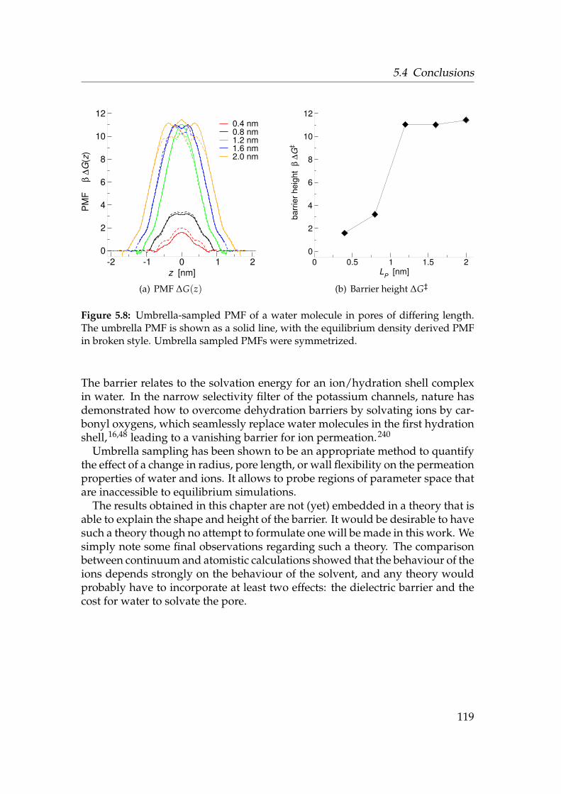
5.4 Conclusions
-2 -1 0 1 2z [nm]
0
2
4
6
8
10
12
PM
F
β ∆G
(z)
0.4 nm0.8 nm1.2 nm1.6 nm2.0 nm
(a) PMF ∆G(z)
0 0.5 1 1.5 2LP [nm]
0
2
4
6
8
10
12
barr
ier h
eigh
t β
∆G+ +
(b) Barrier height ∆G‡
Figure 5.8: Umbrella-sampled PMF of a water molecule in pores of differing length.The umbrella PMF is shown as a solid line, with the equilibrium density derived PMFin broken style. Umbrella sampled PMFs were symmetrized.
The barrier relates to the solvation energy for an ion/hydration shell complexin water. In the narrow selectivity filter of the potassium channels, nature hasdemonstrated how to overcome dehydration barriers by solvating ions by car-bonyl oxygens, which seamlessly replace water molecules in the first hydrationshell,16,48 leading to a vanishing barrier for ion permeation.240
Umbrella sampling has been shown to be an appropriate method to quantifythe effect of a change in radius, pore length, or wall flexibility on the permeationproperties of water and ions. It allows to probe regions of parameter space thatare inaccessible to equilibrium simulations.
The results obtained in this chapter are not (yet) embedded in a theory that isable to explain the shape and height of the barrier. It would be desirable to havesuch a theory though no attempt to formulate one will be made in this work. Wesimply note some final observations regarding such a theory. The comparisonbetween continuum and atomistic calculations showed that the behaviour of theions depends strongly on the behaviour of the solvent, and any theory wouldprobably have to incorporate at least two effects: the dielectric barrier and thecost for water to solvate the pore.
119


6 A gate in the nicotinic receptor
The potential of mean force (PMF) of sodium and chloride ionspermeating the nAChR pore (formed by the pore lining M2 helicesfrom the 4 A closed-state structure) was calculated by fully atom-istic molecular dynamics equilibrium simulations and free energycalculations (umbrella sampling). It is found that ions would haveto overcome a sizable free energy barrier of about 10 kT at the hy-drophobic girdle between residues L9′ and V13′, which has beenimplicated in forming a “hydrophobic gate” at the centre of thepore. The other major constriction, close to the intracellular side,presents a lower barrier so that on the basis of these calculations itis suggested that the gate in the nicotinic receptor is located at thehydrophobic ring. Charged rings at both ends of the pore act asconcentrators of ions up to about six times the bulk concentration;an effect which would increase the ion current in the open state.The influence of different MD force fields and the reduction of theprotein to the M2 bundle is discussed; the general findings are ro-bust with respect to different force fields though the PMFs differin some regions.
The central question pursued so far has been how the pore environment influ-ences the behaviour of water (and ions). The dimensions of the toy pore modelsof Chapter 4 were modelled after what was known from the lower resolutionstructure of the nicotinic acetylcholine receptor (nAChR) at the time.58,59,65,265
The advent of the 4 A structure of the transmembrane domain29 in 2003 allowedus to compare the highly simplified toy model environment to the realistic oneof the ion channel.
6.1 The nicotinic acetylcholine receptor
Nicotinic acetylcholine receptors are membrane channels that mediate signaltransduction at the post-synaptic membrane of cholinergic synapses such asthe neuromuscular junction.266 They belong to the ligand-gated ion channels(LGIC).
121

6 A gate in the nicotinic receptor
6.1.1 The ligand gated ion channels
The ligand gated ion channels comprise of five different known families, fourof which form a sequence-related superfamily (INTERPRO 267 entry IPR006029).These are the gamma-aminobutyric acid type A (GABAA), nicotinic acet-ylcholine (ACh), glycine, and the serotonin (5-hydroxytryptamine, 5HT3) re-ceptors. The ionotropic glutamate receptors (IPR001320) have a distinct primarystructure.
The members of this superfamily share a common architecture. Theyare pentameric complexes of varying subunit composition (for instance, themuscle nAChR of the electric ray Torpedo contains four different subunits α2βγδwhereas the α7 receptor is a homo pentamer). A pore runs through the centreof the complex. Each subunit contains a large N-terminal domain, which con-tains the ligand binding site, three hydrophobic transmembrane (TM) regions,a large intracellular region, and a fourth hydrophobic TM region at the C-terminus.266,268 Based on the structure of the muscle nAChR from Torpedo mar-morata one can confidently identify the TM regions with four membrane span-ning α-helices M1–M429 and the ligand binding domain with a structure madeup mainly from β-sheets.60 The nicotinic receptor ligand binding domain is aspecialised pocket of aromatic and hydrophobic residues formed at interfacesbetween protein subunits that changes conformation to convert agonist bindinginto gating of the ion channel.29,269 The intracellular domain forms a sphere-likevestibule with five windows59,265 but could not be resolved at atomic resolu-tion.
An alignment of the transmembrane domain of the ligand gated ionchannels was prepared, based on the Pfam (“protein family”) PF02932(Neurotransmitter-gated ion-channel transmembrane region), which contains616 members (version 14.0 of PFAM 270). After removal of fragmentary se-quences 511 remained which were aligned with ClustalW.271 A calculation ofan average distance neighbour joining tree (using Jalview272) shows four dis-tinct families (nAChR, 5HT3, GABAA, GlyR) for the whole alignment. Focusingon the M2 region three distinct families remain: nAChR (234 sequences), 5HT3(20 sequences), and GABA/GlyR (244 sequences). From the M2 sequences se-quence logos273 were created, which are shown in Fig. 6.1 on the next page.In the M2 region, the ligand gated ion channels have a number of features incommon: two highly conserved hydrophobic residues at positions 8′ and 9′
(nAChR and 5HT3: LL, GABA/GlyR: VL; L9′ corresponds to αL251 in nAChR),basic residue at −1′ (nAChR: K, 5HT3 and GABA/GlyR: R) with a subsequenthydrophobic one (V1′) at the beginning of the M2 helix. The nAChR and 5HT3receptors are cation selective ion channels. Their sequences exhibit features thatare absent in the GABA/GlyR family, such as the long hydrophobic stretch 13′–18′ (VFLLLI or VFLIIV), the intermediate acidic ring (E at −2′), and the extra-
122
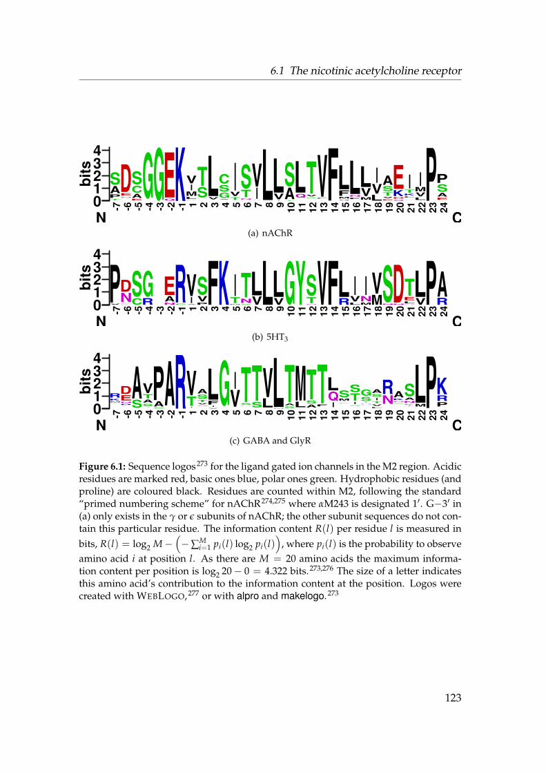
6.1 The nicotinic acetylcholine receptor
01234
bits
N
-7
TPAS
-6
K
N
ED
-5
EACS
-4
G-3
G-2
QE
-1
K1
C
LM
IV
2G
ST
3
VL
4
A
GSC
5
TVI
6
NTS
7
A
IV
8
L9
I
VL
10
T
AS
11
QL
12
S
VT
13
I
F
V
14
F
15
Q
MFL
16
FNL
17
MVL
18
LVI
19
EVTSA
20
Q
DKE
21
S
R
L
KTI
22
LVM
I
23
P
24
EASP
C(a) nAChR
01234
bits
N
-7
VP
-6
K
E
ND
-5
CS
-4
RG
-3 -2
NAE
-1
CR
1
A
IV
2
PVS
3
F4
K5
M
TI
6
S
NT
7
VL
8
L9
VL
10G
11Y
12N
TS
13
V14
F15
RL
16
LVI
17
MN
I
18
MV
19
N
S
20
ND
21
Q
LET
22
VL
23
P
24
RA
C(b) 5HT3
01234
bits
N
-7
P
Y
M
KR
-6
K
R
N
ED
-5
SA
-4
I
SATV
-3
S
AP
-2
A
-1
R
1
I
TV
2
G
VTSA
3
V
IFL
4
G
5
VI
6
M
N
ST
7
ST
8
LV
9
M
L
10
SAT
11
LM
12
AST
13
FT
14
IQL
15
N
F
I
MS
16
G
ITS
17
N
H
I
SG
18
L
VTISA
19NR
20S
N
KA
21T
K
NAS
22
ML
23
P24
PRK
C(c) GABA and GlyR
Figure 6.1: Sequence logos273 for the ligand gated ion channels in the M2 region. Acidicresidues are marked red, basic ones blue, polar ones green. Hydrophobic residues (andproline) are coloured black. Residues are counted within M2, following the standard“primed numbering scheme” for nAChR274,275 where αM243 is designated 1′. G−3′ in(a) only exists in the γ or ε subunits of nAChR; the other subunit sequences do not con-tain this particular residue. The information content R(l) per residue l is measured inbits, R(l) = log2 M−
(−∑M
i=1 pi(l) log2 pi(l))
, where pi(l) is the probability to observeamino acid i at position l. As there are M = 20 amino acids the maximum informa-tion content per position is log2 20− 0 = 4.322 bits.273,276 The size of a letter indicatesthis amino acid’s contribution to the information content at the position. Logos werecreated with WEBLOGO,277 or with alpro and makelogo.273
123

6 A gate in the nicotinic receptor
cellular acidic rings (E or D at 20′ and 24′).The nicotinic receptor is one of the best studied ion channels and serves as
a pardigm for ligand gated ion channels. The muscle-type receptor facilitatessignal transduction from motor neurons to muscle cells and is located in thepost synaptic membrane of a muscle cell; neuronal nAChR such as the α7 re-ceptor (discussed briefly in Appendix A) are found in brain synapses. nAChRis a cation selective ion channel with conductances of the order of 30 pS.12 Itsnatural agonist is acetylcholine (ACh) but it binds nicotine at even higher affin-ities.
6.1.2 Structure of the pore
The nicotinic receptor is the only membrane channel of which a structure isknown in both the open58 and closed state.29,65 Although the resolution of theopen state structure is comparatively low at 9 A, a wide pore of radius R ≈0.65 nm is visible in the density. This is wide enough to let fully hydrated cationspass. It is also consistent with nAChR being an only weakly selective cationchannel which is permeable to many inorganic cations and at least 41 organiccations and even non-polar molecules like urea, ethylene glycol, or glycerol.12
Because the open and closed structures are known one should be able tolearn something about the gating mechanism of the receptor, and by similar-ity, about the gating mechanism in all related LGICs. The current view, basedon the structure of the receptor itself29,60,278 and the acetylcholine binding pro-tein AChBP,279 which is homologous to the ligand binding domain of nAChR,holds that a structural change in the ligand binding domain, induced by thebinding of two molecules of ACh, is transmitted through the linker region280 tothe M2 helices of the transmembrane region. The M2 helices swing in hinges(in the M2–M3 and M1–M2 linker) to open or close the pore.18,29,61,280 Many de-tails of the gating process are still elusive. Even the seemingly trivial questionwhere the flow of ions is blocked in the closed state—the gate—is debated asbiochemical evidence281,282 (summarised by Karlin275) clashes with structural29
and other biochemical data.283–287
Where is the gate? The structure of Miyazawa et al.29 (at 4 A resolution)is thought to represent the closed state because no agonist was present duringrecording of the electron microscopy images. At this resolution the backbonecould be built into the electron density although most of the sidechains hadto be modelled. The structure unambiguously shows that the M2 helices arelining the ion pathway. The pore is also peculiarly feature-poor without anyprominent sidechains that could act as an occlusion gate (Fig. 6.2(a) on the fa-cing page). Furthermore, the lower resolution images59,265,288 (at about 4.6 A)
124
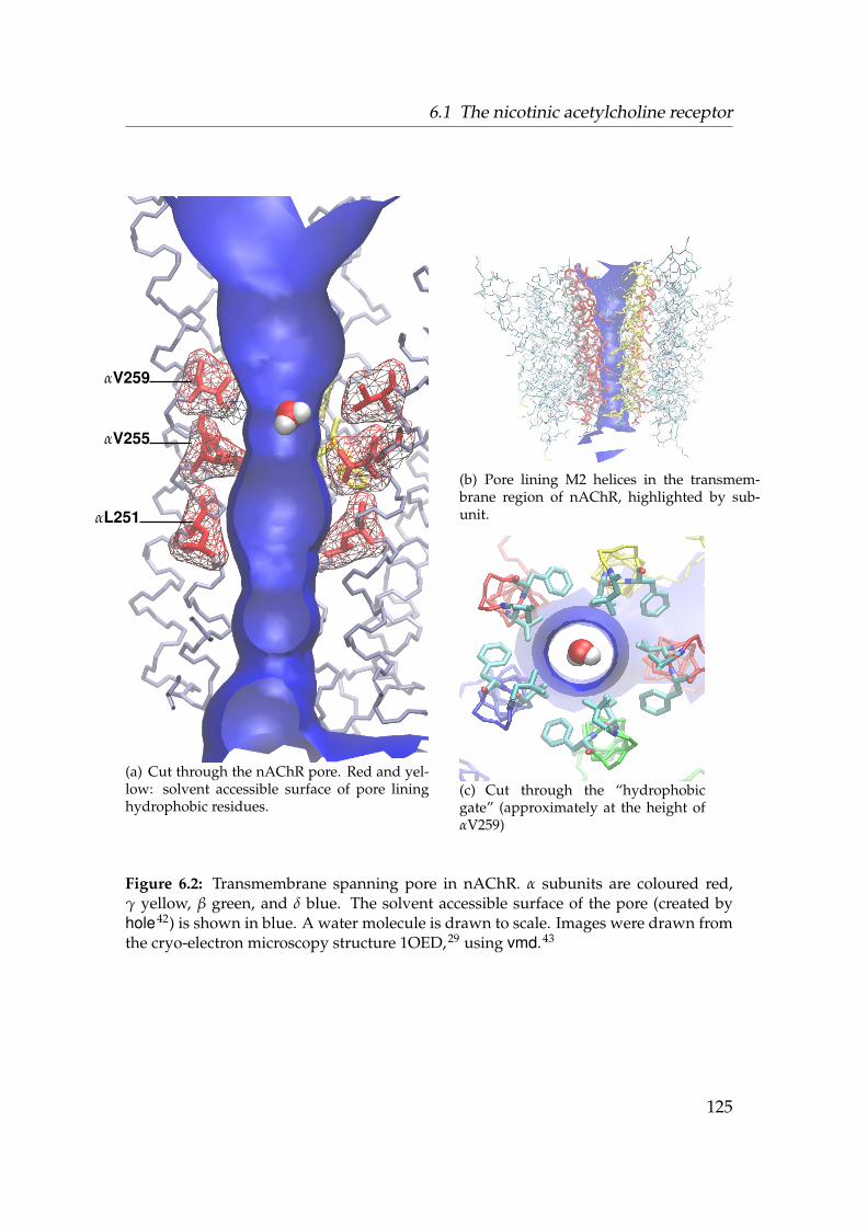
6.1 The nicotinic acetylcholine receptor
αV259
αV255
αL251
(a) Cut through the nAChR pore. Red and yel-low: solvent accessible surface of pore lininghydrophobic residues.
(b) Pore lining M2 helices in the transmem-brane region of nAChR, highlighted by sub-unit.
(c) Cut through the “hydrophobicgate” (approximately at the height ofαV259)
Figure 6.2: Transmembrane spanning pore in nAChR. α subunits are coloured red,γ yellow, β green, and δ blue. The solvent accessible surface of the pore (created byhole42) is shown in blue. A water molecule is drawn to scale. Images were drawn fromthe cryo-electron microscopy structure 1OED,29 using vmd.43
125
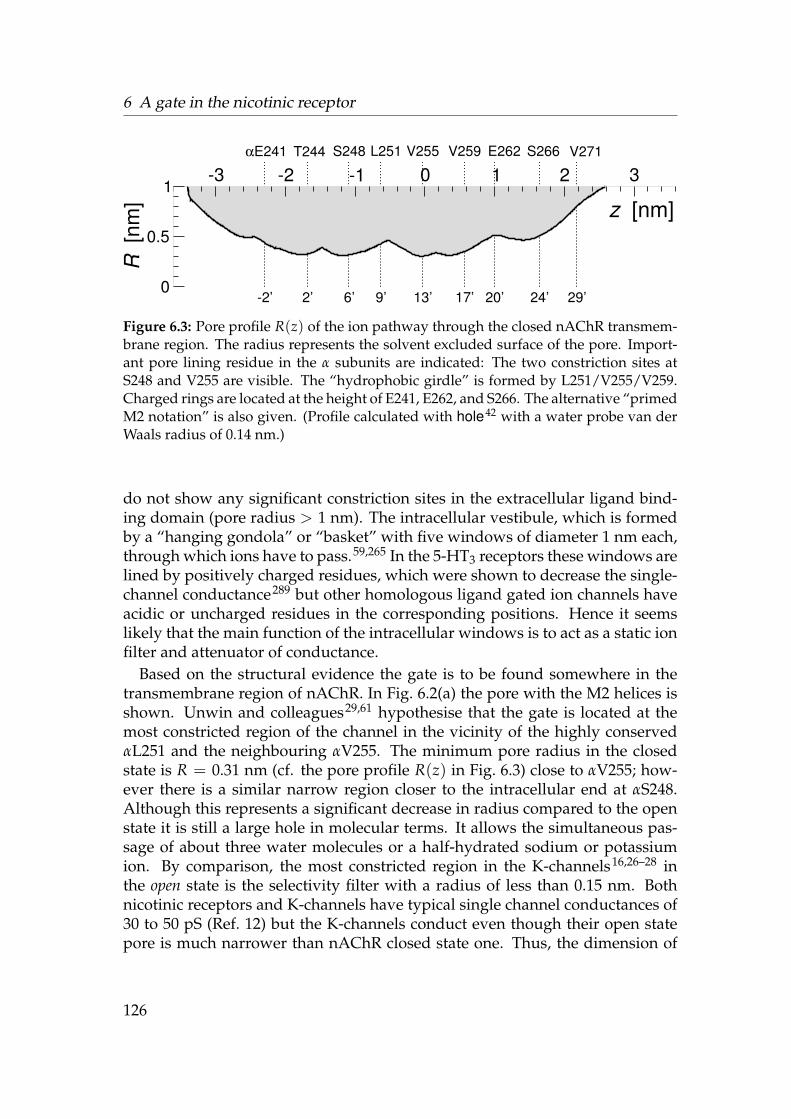
6 A gate in the nicotinic receptor
V255 V259 L251 T244αE241 V271S248 S266 E262
13’ 17’9’2’-2’ 29’6’ 24’20’
-3 -2 -1 0 1 2 3
z [nm]
0
0.5
1
R [
nm]
Figure 6.3: Pore profile R(z) of the ion pathway through the closed nAChR transmem-brane region. The radius represents the solvent excluded surface of the pore. Import-ant pore lining residue in the α subunits are indicated: The two constriction sites atS248 and V255 are visible. The “hydrophobic girdle” is formed by L251/V255/V259.Charged rings are located at the height of E241, E262, and S266. The alternative “primedM2 notation” is also given. (Profile calculated with hole42 with a water probe van derWaals radius of 0.14 nm.)
do not show any significant constriction sites in the extracellular ligand bind-ing domain (pore radius > 1 nm). The intracellular vestibule, which is formedby a “hanging gondola” or “basket” with five windows of diameter 1 nm each,through which ions have to pass.59,265 In the 5-HT3 receptors these windows arelined by positively charged residues, which were shown to decrease the single-channel conductance289 but other homologous ligand gated ion channels haveacidic or uncharged residues in the corresponding positions. Hence it seemslikely that the main function of the intracellular windows is to act as a static ionfilter and attenuator of conductance.
Based on the structural evidence the gate is to be found somewhere in thetransmembrane region of nAChR. In Fig. 6.2(a) the pore with the M2 helices isshown. Unwin and colleagues29,61 hypothesise that the gate is located at themost constricted region of the channel in the vicinity of the highly conservedαL251 and the neighbouring αV255. The minimum pore radius in the closedstate is R = 0.31 nm (cf. the pore profile R(z) in Fig. 6.3) close to αV255; how-ever there is a similar narrow region closer to the intracellular end at αS248.Although this represents a significant decrease in radius compared to the openstate it is still a large hole in molecular terms. It allows the simultaneous pas-sage of about three water molecules or a half-hydrated sodium or potassiumion. By comparison, the most constricted region in the K-channels16,26–28 inthe open state is the selectivity filter with a radius of less than 0.15 nm. Bothnicotinic receptors and K-channels have typical single channel conductances of30 to 50 pS (Ref. 12) but the K-channels conduct even though their open statepore is much narrower than nAChR closed state one. Thus, the dimension of
126

6.1 The nicotinic acetylcholine receptor
240. 245. 250. 255. 260. 265. 270.240 G-EKMTLSISVLLSLTVFLLVIVELIPSTSSAVP α246 G-EKMSLSISALLAVTVFLLLLADKVPETSLSVP β250 GGQKCTLSISVLLAQTIFLFLIAQKVPETSLNVP γ254 G-EKMSTAISVLLAQAVFLLLTSQRLPETALAVP δ
gate ?
Figure 6.4: Alignment of the M2 stretches from the Torpedo californica nAChR sub-units. The ruler counts residues in the α subunit. In the “primed M2 notation” ofLester274, αM243 is 1′, the start of the M2 helix. αL251 corresponds to 9′ and αV255 to13′. The gate as proposed by Miyazawa et al.29 is indicated between αL251 and αV259.Hydrophobic residues are coloured in green, or black (as pore lining hydrophobic
residues). Acidic (positively charged) residues are coloured red, basic (negat-ively charged) blue and polar uncharged ones yellow. (Alignment typeset withTEXshade290)
the pore alone can not determine the conductance properties. Hille12 sensiblysuggests that the interaction of the ion with the pore wall must play a decisiverole in shaping the conductance and selectivity properties of ion channels.
The K-channel selectivity filter is lined by eight backbone carbonyl oxygenatoms of the TVGYG signature motif.16,26–28,237 These oxygens substitute forwater molecules in the hydration shell of a permeating ion. The situation ap-pears to be different for the nicotinic receptor. The sequence of the pore lin-ing M2 helices (Fig. 6.4) shows a number of hydrophobic residues, and in factlarge parts of the pore are exclusively lined by leucines and valines (Fig. 6.2(a)).Thus it appears unlikely that a similar water-substitution mechanism wouldhelp ions to move through the pore. Furthermore, as was demonstrated in theprevious chapters for the case of hydrophobic model pores, the presence of a hy-drophobic pore lining surface appears to be the mechanism which prevents ionsfrom permeating the hydrophobic girdle. The MD simulations of this chapterare aimed at testing this hypothesis.
Not only is the central region of the pore lined by hydrophobic residuesbut also does the complete stretch L251–V259 consist of hydrophobic residues.These form a compact dielectric plug at the centre of the membrane, whichmight contribute to an increase in the Born barrier.
The TM region is flanked by rings of acidic residues. Three of these rings areclearly visible in the sequence logo for the nicotinic receptors, Fig. 6.1(a). Theintracellular ring at position −6′ lies in the M2-M3 linker.275 The intermediate
127
6 A gate in the nicotinic receptor
ring at−2′ and the extracellular ring at 20′, however, are directly lining the pore(see also Fig. 6.4 for the identities of the corresponding residues in the differentsubunits). Some nicotinic receptors (notably the muscle nAChR and the α7 one)have a fourth charged ring at position 24′. There are no charged residues withinthe membrane, where the position of the membrane is inferred from belts ofaromatic residues (Fig. 6.5 on the next page shows the position of the chargedresidues relative to the aromatic belts and hence relative to the membrane). Allcharged sidechains are located in the lipid head group region or above. A highlynegatively charged channel lumen is expected for a cation selective channel likethe nicotinic receptor or the closely related 5-HT3 receptors (cf. Fig. 6.1(b) andFig. 6.1(a)); anion-selective channels like the GABA and Glycine receptors intro-duce positively charged rings at 19′ and 24′ instead (Fig. 6.1(c)). It is suggestedthat charged vestibules can act as ionic concentrators, which in turn increasesconductance.12
6.1.3 Identifying the gate
Based on the knowledge of the structure of Torpedo marmorata nAChR in theclosed state we wish to identify the gate, i.e. the region of the pore which pre-vents ions from permeating the pore. As argued in the previous section, wehypothesise that the gate is to be found in the transmembrane spanning pore.This inference is based on the knowledge of static structures. The experiencewith the dynamics of ion permeation in model pores, described in the previouschapters, strongly implicates the hydrophobic constriction site formed in thevicinity of αV255, βL261, γI264, and δL269. In this chapter we test our hypo-thesis by carrying out atomically detailed molecular dynamics simulations ofions in the nAChR pore. In particular, we compute the PMF of ions permeatingthe receptor pore; our calculations of the barrier in model pores in Chapter 5demonstrated the applicability of this approach. Also, our previous calcula-tions indicated that simulations of more than 50 ns (deemed “long” by currentstandards) are required for proper sampling of equilibrium ionic densities inconfined geometries. In order to reach long simulation times we perform ourcalculations on a reduced model, consisting only of the M2 helices, which isdescribed in detail in 6.2.2.
6.2 Methods
The complete transmembrane region of Torpedo marmorata nAChR (pdb code1OED), which was solved by cryo electron microscopy (cryo-EM) to about 4 Aresolution,29 was taken as the initial structure.
128
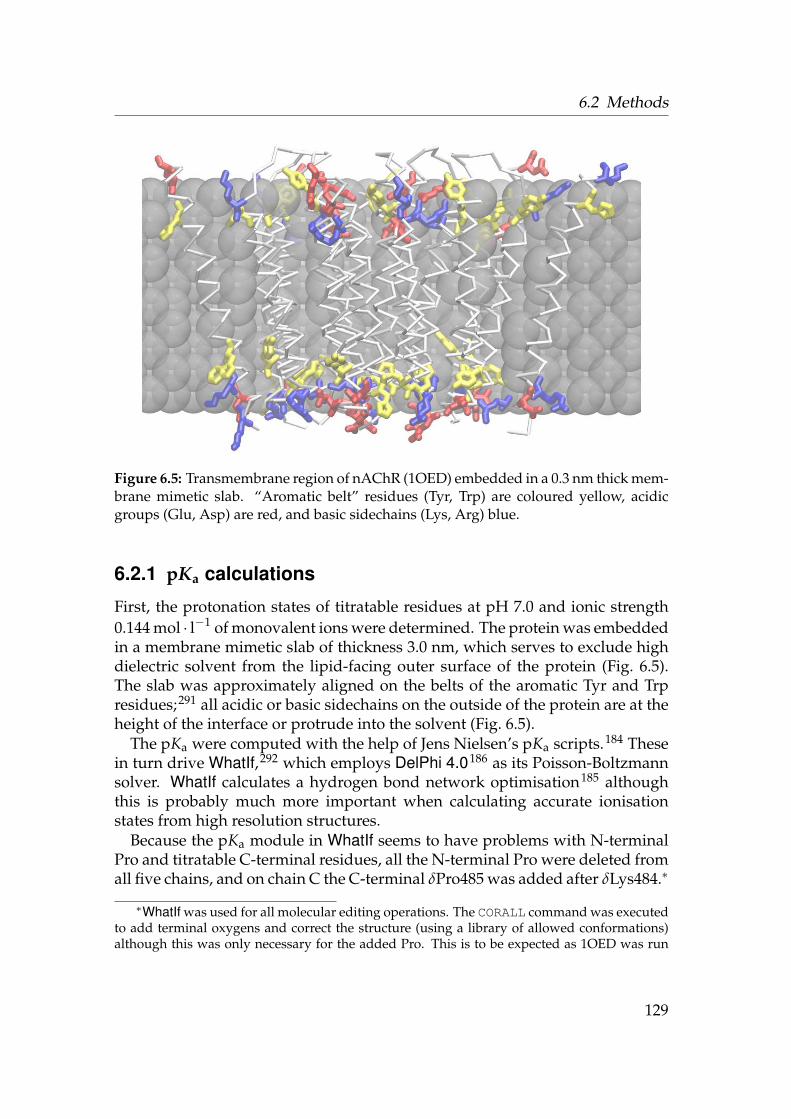
6.2 Methods
Figure 6.5: Transmembrane region of nAChR (1OED) embedded in a 0.3 nm thick mem-brane mimetic slab. “Aromatic belt” residues (Tyr, Trp) are coloured yellow, acidicgroups (Glu, Asp) are red, and basic sidechains (Lys, Arg) blue.
6.2.1 pKa calculations
First, the protonation states of titratable residues at pH 7.0 and ionic strength0.144 mol · l−1 of monovalent ions were determined. The protein was embeddedin a membrane mimetic slab of thickness 3.0 nm, which serves to exclude highdielectric solvent from the lipid-facing outer surface of the protein (Fig. 6.5).The slab was approximately aligned on the belts of the aromatic Tyr and Trpresidues;291 all acidic or basic sidechains on the outside of the protein are at theheight of the interface or protrude into the solvent (Fig. 6.5).
The pKa were computed with the help of Jens Nielsen’s pKa scripts.184 Thesein turn drive WhatIf,292 which employs DelPhi 4.0186 as its Poisson-Boltzmannsolver. WhatIf calculates a hydrogen bond network optimisation185 althoughthis is probably much more important when calculating accurate ionisationstates from high resolution structures.
Because the pKa module in WhatIf seems to have problems with N-terminalPro and titratable C-terminal residues, all the N-terminal Pro were deleted fromall five chains, and on chain C the C-terminal δPro485 was added after δLys484.∗
∗WhatIf was used for all molecular editing operations. The CORALL command was executedto add terminal oxygens and correct the structure (using a library of allowed conformations)although this was only necessary for the added Pro. This is to be expected as 1OED was run
129

6 A gate in the nicotinic receptor
Interactions between titratable groups were only computed if the electrostaticinteraction in the fully charged state exceeded a “pair energy cutoff” of 4 kT.184
Test calculations on other systems (OpcA and OmpX) showed that this is anacceptable simplification.
6.2.2 Models
As we want to investigate how the environment affects the behaviour of waterand ions we are not concerned with large scale protein motions but only localproperties of the water/wall interface. Thus major simplifications are carriedout to reduce the system size, which is important to achive long simulationtimes for accurate sampling of water and especially ion trajectories.
1. The outer transmembrane helices M1, M3 and M4 (the “scaffold”) wereremoved using WhatIf. Only the full length M2 helices with some residuesfrom the M1-M2 and M2-M3 linker were retained (αE241 to αV271). Themodel contained 31 residues in each chain and stretched over a length of5 nm. The resulting structure was called the P1 model.∗
2. Because the reduced pore model lacks stabilising contacts with the outerscaffold and with the ligand binding domain the backbone atoms were re-strained to their position determined by cryo-EM,† similar to the approachadopted by Smith and Sansom171 for PMF calculations in leucine-serinepeptides.
3. Once the equilibrium position of the backbone is fixed we can also sim-plify the treatment of the lipid membrane. The M2 helices would not
through procheck293 before publication and many sidechains were software-built, as can beinferred, for instance, from the REMARK section of 1OED.pdb:
[. . . ] These coordinates, including estimates of side chain positions, are beingmade available in the hope that they will be useful. Users should bear in mindthat because of the limited resolution the conformations of the side chains andtheir atomic coordinates are not individually reliable. [. . . ]
The edited structure was only used for the pKa calculations.∗A so-called P4 model was also constructed for initial test calculations. It consisted of the
hydrophobic pore itself (from αI247 to αV259) (13 residues, length 2.1 nm). P2 and P3 weredesigned as intermediates but were never used.†In fact, there are NMR studies of an M2 only channel in a bilayer294 and corresponding MD
simulations.295,296 The MD simulations showed some significant changes in the pore geometry.For the purpose of the present study it was deemed necessary to keep the pore geometry welldefined. In essence, it is assumed that the experimental structure is a good representation of theclosed state and on the time scales accessible to MD no larger rearrangements or destabilisationswould likely occur.
130
6.2 Methods
be in contact with lipids in the full receptor and any lipid-protein in-teractions would be countered by the backbone restraints. Although areal lipid membrane contains polar head groups, which may have a longrange electrostatic effect on ion permeation this can likely be ignored inthis particular case: In the complete receptor, the scaffold shields the per-meation pathway from the head groups. The minimum distance for a lipidhead group from the pore surface is 2 nm, as estimated from the solvent-accessible surface121 of the structure 1OED in vmd.43 It also contains cavit-ies which are most likely be filled with water (see Section 6.3.3), which canscreen electrostatic fields effectively. Thus it appears acceptable to leaveout the polar head groups and model the membrane by a low dielectricslab made from methane molecules, as was done for the model pores inthe previous chapters.
The final model is suitable to investigate the question how the environment ofthe closed nAChR pore affects ions and water under the assumption that theclosed pore is correctly described by the cryo-EM structure 1OED.
6.2.3 Poisson-Boltzmann calculations
The Born profile for a Na+ ion in the nAChR pore was calculated analogously tothe model pores in Section 5.2.3 on page 110 with a few variations to account forthe presence of the protein. Hydrogen atoms were added to the input structure(either 1OED or P1) with WhatIf292. The resulting structure was embedded in amembrane mimetic slab.∗ The ion was positioned on the pore axis (calculatedwith hole42) in steps of 0.02 nm and extended for 1.5 nm into the bulk. ThePDB2PQR 297 server was used to build an input file for the Poisson-Boltzmannsolver apbs.179 Protein radii and partial charges were taken from the AMBERforce field† (as provided by PDB2PQR) and a Born radius of 0.1680 nm was usedfor the Na+ ion.181 Poisson-Boltzmann calculations—as described in Section 2.4on page 54—were carried out on a grid of dimensions 65× 65× 97 with multiplefocusing steps into an area of size 1 nm× 1 nm× 1 nm, centred on the positionof the test ion. The temperature was set to T = 300 K, the dielectric constant ofthe solvent was taken to be ε = 78.5 and εp = 2.0 for the protein/membranemimetic; the ionic strength of the solution was set to 1 mol · l−1 with Stern radiirNa+ = 0.095 nm and rCl− = 0.181 nm, and the radius of an implicit solvent
∗Test calculations on a model of the α7 receptor actually showed negligible dependence onthe presence of a membrane mimetic (Kaihsu Tai, personal communication).†The OPLS-AA force field was in part derived from AMBER so choosing AMBER for the
Poisson-Boltzmann calculations should facilitate comparison between the MD with OPLS-AAand the PB free energy profiles.
131

6 A gate in the nicotinic receptor
Table 6.1: Equilibrium simulations of nAChR M2 (P1 model). GROMOS96 (G43A1) isan united atom force field, only including polar hydrogens, whereas OPLS-AA modelsall hydrogen atoms explicitly. kbb is the strength of the restraints on the backbone of theM2 helices, measured in k0 = 1.0× 10³ kJ ·mol−1 · nm−2. Simulations were typicallycarried out for a total run length of T in a NaCl solution of nominal concentrationc(NaCl). Each system contained N atoms in total (including hydrogens).
force field water kbb/k0 c(NaCl)/mol · l−1 T/ns N
GROMOS96 SPC 0.2 1.0 80 107291.0 — 80 107731.0 0.2 80 105571.0 1.0 80 10557
OPLS-AA SPC 1.0 1.0 60 15298TIP4P 1.0 1.0 55 18002
molecule 0.14 nm. The Born energy was calculated according to Eq. (2.115) onpage 56.
6.2.4 Molecular Dynamics
Equilibrium properties of ions and water were studied both by equilibrium MDand biased MD simulations (umbrella sampling along the pore axis) with theaim of determining the density n(z) and the PMF G(z).
MD simulations were performed with gromacs version 3.1.4 or version3.2.1127 and the SPC water model132 or TIP4P.144,145 Calculations were car-ried out with two different force fields. Initially, the united atom forcefield GROMOS96 (G43A1)132,133 was employed for equilibrium and umbrellasampling simulations. However, the question arose if explicit representationsof hydrogens might be important. Hence the previous simulations were re-peated with the all atom OPLS-AA/L 134,140 force field. The integration time stepwas 2 fs.∗ In both cases, explicit hydrogens were “dummified”, i.e. their pos-ition is calculated from the geometry of the surrounding heavy atoms and notby forces on the H themselves, thus removing fast degrees of freedom. Typ-ical simulations employed the following parameters; for variations see the listof equilibrium simulations of the P1 system in Tab. 6.1. Backbone atoms were
∗Larger time steps were also explored. ∆t = 5 fs steps with GROMOS96 run stably but thebehaviour of the water in the pore was qualitatively different from the ∆t = 2 fs runs. Waterevaporated much more readily from the gate region in the 5 fs simulations. It was decided thataccurate representation of the solvent is important in our simulations and hence a (canonical)∆t = 2 fs was used.
132

6.2 Methods
Table 6.2: Parameters of the Umbrella sampling simulations. kbb is the spring constantof the backbone restraints on the P1 model of the nAChR TM pore. Umbrella samplingof an ion or a water molecule proceeded for a time T after an equilibration phase oflength Teq. Altogether N windows of length ∆z were sampled with a harmonic poten-tial of force constant k. k0 = 1.0× 10³ kJ ·mol−1 · nm−2. All simulations employed theSPC water model.
force field kbb/k0 species T/ns Teq/ns N ∆z/nm k/k0
GROMOS96 0.2 Na+ 0.5 0.1 101 0.0495 0.9971.0 water 0.5 0.1 101 0.0544 0.824
Na+ 1.0 2.0 200 0.025 3.910Cl− 1.0 2.0 101 0.0495 0.997
OPLS-AA 1.0 water 1.0 0.2 101 0.0396 1.558Na+ 1.0 0.2 101 0.0396 1.558Cl− 1.0 0.2 101 0.0396 1.558
restrained171 with kbb = k0 = 4.0 kT A−2 = 1.0× 10³ kJ ·mol−1 · nm−2 (ex-cept for one simulation at kbb = 0.2 k0), giving them roughly the same posi-tional root mean square fluctuation as seen in simulations of potassium chan-nels.201 Coordinates were saved every 2 ps. With periodic boundary conditions,long range electrostatic interactions were computed with a particle mesh Ewaldmethod (real space cutoff 1 nm, grid spacing 0.15 nm, fourth order interpola-tion164,165) while the short ranged van der Waals forces were calculated withina radius of 1.4 nm. The neighbour list (radius 1 nm) was updated every 10steps. Weak coupling algorithms166 were used to maintain constant temperat-ure (T = 300 K, time constant 0.1 ps) and pressure (P = 1 bar, compressibility4.5× 10−5 bar−1, time constant 1 ps) with the x and y dimensions of the simu-lation cell held fixed at 4.6 nm. The length in z was 8.5 nm (ensuring bulk-likewater behaviour far from the membrane mimetic and the protein surface). TheP1 system contained about 500 methane pseudo-atoms (or methane moleculesfor the all atom force field), which form the membrane mimetic, 3000 SPC wa-ter molecules and about 1400 heavy atoms. It was simulated for 80 ns withGROMOS96 and between 55 ns and 60 ns for OPLS-AA (see Tab. 6.1 for details).
Umbrella sampling Umbrella sampling172 was carried out as described inSection 2.3.2. Parameters of the different simulation runs are listed in Tab. 6.2.The biased histograms were unbiased with WHAM.175 Umbrella-sampledPMFs and PMFs from long equilibrium simulations were manually combinedso that the barrier height, i.e. the free energy difference between a particlein bulk and at the centre of the barrier, could be determined. The umbrella-
133
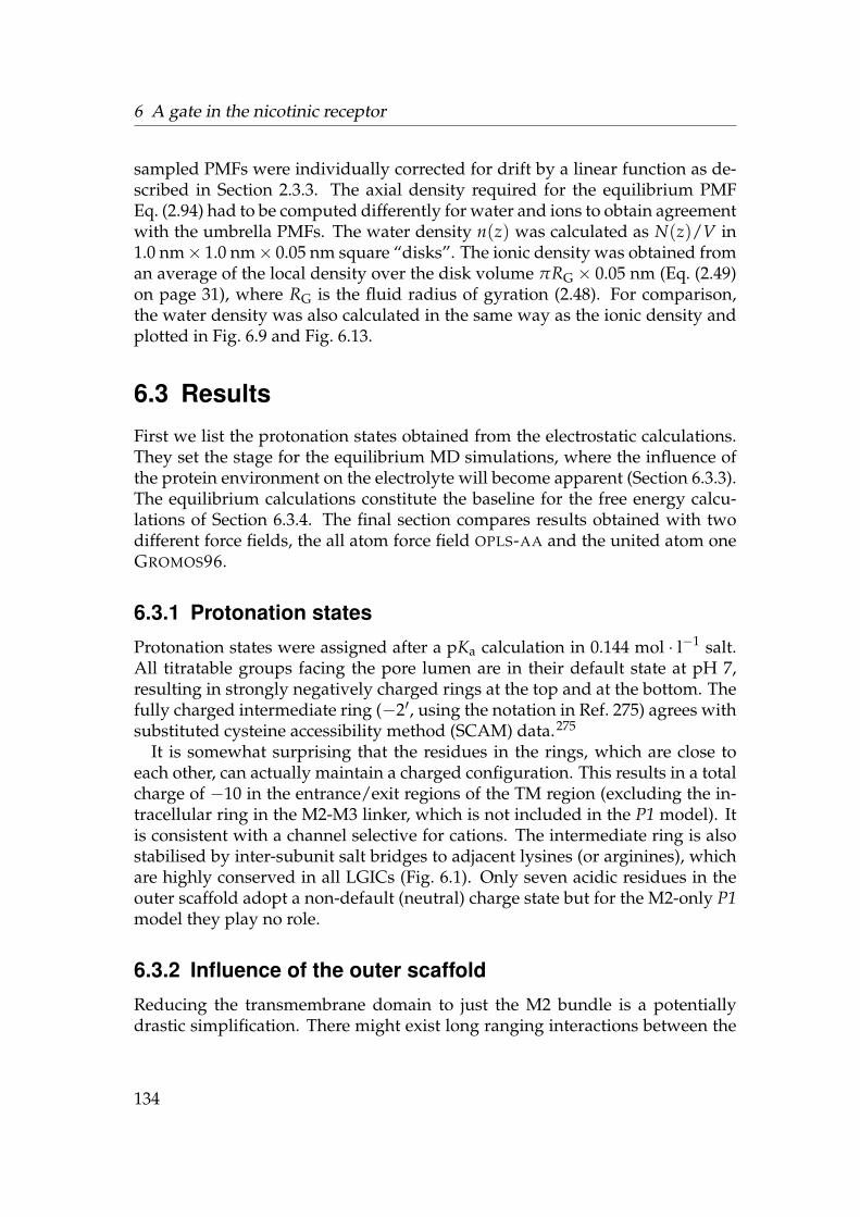
6 A gate in the nicotinic receptor
sampled PMFs were individually corrected for drift by a linear function as de-scribed in Section 2.3.3. The axial density required for the equilibrium PMFEq. (2.94) had to be computed differently for water and ions to obtain agreementwith the umbrella PMFs. The water density n(z) was calculated as N(z)/V in1.0 nm× 1.0 nm× 0.05 nm square “disks”. The ionic density was obtained froman average of the local density over the disk volume πRG × 0.05 nm (Eq. (2.49)on page 31), where RG is the fluid radius of gyration (2.48). For comparison,the water density was also calculated in the same way as the ionic density andplotted in Fig. 6.9 and Fig. 6.13.
6.3 Results
First we list the protonation states obtained from the electrostatic calculations.They set the stage for the equilibrium MD simulations, where the influence ofthe protein environment on the electrolyte will become apparent (Section 6.3.3).The equilibrium calculations constitute the baseline for the free energy calcu-lations of Section 6.3.4. The final section compares results obtained with twodifferent force fields, the all atom force field OPLS-AA and the united atom oneGROMOS96.
6.3.1 Protonation states
Protonation states were assigned after a pKa calculation in 0.144 mol · l−1 salt.All titratable groups facing the pore lumen are in their default state at pH 7,resulting in strongly negatively charged rings at the top and at the bottom. Thefully charged intermediate ring (−2′, using the notation in Ref. 275) agrees withsubstituted cysteine accessibility method (SCAM) data.275
It is somewhat surprising that the residues in the rings, which are close toeach other, can actually maintain a charged configuration. This results in a totalcharge of −10 in the entrance/exit regions of the TM region (excluding the in-tracellular ring in the M2-M3 linker, which is not included in the P1 model). Itis consistent with a channel selective for cations. The intermediate ring is alsostabilised by inter-subunit salt bridges to adjacent lysines (or arginines), whichare highly conserved in all LGICs (Fig. 6.1). Only seven acidic residues in theouter scaffold adopt a non-default (neutral) charge state but for the M2-only P1model they play no role.
6.3.2 Influence of the outer scaffold
Reducing the transmembrane domain to just the M2 bundle is a potentiallydrastic simplification. There might exist long ranging interactions between the
134

6.3 Results
Table 6.3: Protonation states of titratable residues in M2 at pH 7. There are four acidicrings at the height or above the bilayer surface. Negatively charged sidechains are setin bold type. Residues are counted within M2 by the primed numbering scheme whichdesignates αM243 the number 1′.274,275 Numbering of residues is taken from the pdbfile 1OED.29 The second extracellular ring at 24′ is specific to some nicotinic receptorslike the muscle nAChR or the α7 receptor.
Description Position charge αδ γ αγ β δ
(2nd EC ring) 24′ −3 S266 E275 S266 E272 E280extracellular ring 20′ −3 E262 Q271 E262 D268 Q276intermediate ring −2′ −4 E241 Q250 E241 E247 E255intracellular ring −5′ −4 D238 Q246 D238 D244 E252
scaffold (the M1, M3, and M4) helices and the ion pathway, which affect per-meation. (We are not concerned with interactions that position the M2 helicesbecause this effect is approximated by restraining the M2 backbone to the EMstructure positions.)
Long range effects would most likely be dominated by electrostatic effects.In order to assess the significance of the outer scaffold for ion permeation, theelectrostatic PMF (or Born profile) of a Na+ ion was calculated for the full TMdomain and the M2 bundle (the P1 model) only. As Fig. 6.6 shows, the differ-ence in electrostatic free energy between the P1 model and the full TM domainis negligible. The only region where differences are detectable is at the intra-cellular end where ions in the full TM domain are stabilised by about 0.5 kTcompared to the M2 bundle. This is due to the intracellular ring (cf. Tab. 6.3),which carries a charge of −4e in the full structure but which is absent in the M2bundle. Thus, the influence of the scaffold is shown to be very small, whichlends some justification to proceeding with the M2 helix bundle model.
Another potentially serious simplification is the omission of the synaptic (ex-tracellular) ligand binding (LB) domain. For the Torpedo nAChR there is nomodel available that contains both TM and LB domains.∗ Recently a homologymodel of the α7 receptor (another member of the family of nicotinic receptors)was presented,41 which only misses the intracellular domain. Preliminary cal-culations for the electrostatic PMF in the α7 receptor indicate that the LB do-main does have an influence on the Born profile (see Appendix A). The barriersare consistently higher in the presence of the LB domain than in their absence(Fig. A.2). It is expected that this is also the case for Torpedo nAChR, even though
∗The structure of the intracellular basket or hanging gondola is not known at atomic resolu-tion though it is possible to capture general characteristics like dimensions, openings, or chargedecoration in coarse grained models, based on pseudo-atoms (O. Beckstein, unpublished).
135
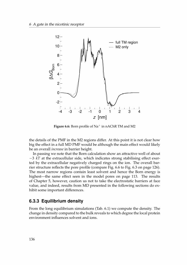
6 A gate in the nicotinic receptor
-4 -3 -2 -1 0 1 2 3 4z [nm]
-2
0
2
4
6
8
10
12
β∆G
Bor
n
full TM regionM2 only
Figure 6.6: Born profile of Na+ in nAChR TM and M2
the details of the PMF in the M2 regions differ. At this point it is not clear howbig the effect in a full MD PMF would be although the main effect would likelybe an overall increase in barrier height.
In passing we note that the Born calculation show an attractive well of about−3 kT at the extracellular side, which indicates strong stabilising effect exer-ted by the extracellular negatively charged rings on the ion. The overall bar-rier structure reflects the pore profile (compare Fig. 6.6 to Fig. 6.3 on page 126).The most narrow regions contain least solvent and hence the Born energy ishighest—the same effect seen in the model pores on page 113. The resultsof Chapter 5, however, caution us not to take the electrostatic barriers at facevalue, and indeed, results from MD presented in the following sections do ex-hibit some important differences.
6.3.3 Equilibrium density
From the long equilibrium simulations (Tab. 6.1) we compute the density. Thechange in density compared to the bulk reveals to which degree the local proteinenvironment influences solvent and ions.
136

6.3 Results
0.15
0.30
0.60
0.90
1.20
1.50
1.80
2.10
2.40
2.70
3.00
3.30
3.60
3.90
4.20
striction,Lower con−
S248 (6’)
1 nm1 nm
LCG
G
C
L
Gate,V255 (13’)
Cavity,L251:O (9’)
Water density in units ofSPC water at 1 bar, 300K
β
δγ
αδ
αγ
Figure 6.7: Water density in nAChR. The putative hydrophobic gate29 G is formed byhydrophobic sidechains (αV255–αV259). C designates the “cavity”, lined by backbonecarbonyl group of L9′ (αL251), L the lower constriction site formed by Ser and Thrresidues. (Force field GROMOS96 with similar results for OPLS-AA.)
Water Water in the closed receptor is shown in Fig. 6.7. The nAChR pore ismuch more polar than the hydrophobic model pores due to the presence of thebackbone. So it is not too surprising that water can be seen in all regions of thepore.The putative gate region around αV255 is of particular interest. As seen inthe cross section, water density is localised in a pentameric pattern, leaving ahollow tube.This hints at strong constraints for the water position: Water canonly maintain its presence if it interacts in a fairly restrictive configuration.∗
However, these “rings” are not pentameric rings of water molecules hydrogenbonded to each other. The picture only emerges on average. Typically, a stringof water molecules rotates in the pore and the string switches between five dif-ferent favourable positions. Similar behaviour of water was observed in theputative gate region of MscS.56 Inspection of the trajectories also shows evapor-ation and condensation events in the hydrophobic girdle although the vapourphases are shorter than in the case of the model pores.†
A slightly wider region (cavity), which is lined by the backbone oxygens ofαL251, contains water at bulk density. The lower constriction site is seen to bethe narrowest part (for water at least), where water molecules will only stayin very specific locations, namely close to βS250 (between αγ and β, top of
∗Cursory investigation suggests loss of hydrogen bonds above and below the gate.†Anishkin and Sukharev56 observe even more pronounced vapour phases in the putative
hydrophobic gate of MscS and term it a “vapour-plug” or “vapour-lock” mechanism.46,96.
137
6 A gate in the nicotinic receptor
(a) Water (b) Na+ (c) Cl−
Figure 6.8: Radially averaged density of 1.3 mol · l−1 sodium chloride solution in nA-ChR (M2 only, i.e. the P1 model). OPLS-AA force field. which treats all hydrogensexplicitly. The colour scale is the same as in Fig. 4.6 on page 100.
Fig. 6.7L) and in the vicinity of αT244 and γT253.
Ions Equilibrium MD simulations of electrolytes typically suffer from verylong equilibration times. If there are also high barriers for the ions to overcomethen they will not sample all available configurations sufficiently. By using ahigh salt concentration one can achieve more sampling in a given simulationtime. Thus simulations were performed for a nominal 1 mol · l−1 NaCl solution;results for one at 0.2 mol · l−1 NaCl look similar albeit at a lower density, i.e.less frequent presence of ions in the pore. It turns out that the bulk density isnot 1 mol · l−1 even though the number of ions per water molecule was adjus-ted to give this value. The densities from the simulations show a bulk densityof about 1.3 mol · l−1 (Fig. 6.8). The reason lies in the formation of an ion exclu-sion layer near the membrane and protein surface and in the pore itself (cf. thesituation encountered for the model pores in Section 4.3.2). Ions are forced intobulk regions, and, because of the limited size of the simulation box, increase thebulk density noticeably. This is not a problem as long as one uses the real bulkdensity n0 = 1.3 mol · l−1 when calculating the equilibrium PMF Eq. (2.94).
The density of ions in the M2 pore (Fig. 6.8) vanishes in large parts of the poreregion. Effectively, the pore is blocked for both ionic species, which is similar to
138

6.3 Results
V255 V259 L251T244E241 V271S248 E262 S266
-3 -2 -1 0 1 2 3z−zcom [nm]
0
1
2
3
4
5
6
7
n wat
er/n
0an
d n
ion [m
ol/l]
water (LD)waterNa+
Cl−
Figure 6.9: Axial density n(z) in nAChR with the OPLS-AA force field and SPC water.For ions and water (LD), n(z) was computed from the local density n(x) according toEq. (2.49); for water it was calculated from averages in quadratic disks of dimensions1 nm × 1 nm × 0.05 nm. Water density is given in units of the bulk density of SPCwater n0. Important pore lining residues of the P1 model of nAChR are indicated.The hydrophobic girdle lies between V255 and V259 and the lower constriction site islocated at S248. The charged extracellular rings lie at E262 and S266 and carry a totalcharge of −6e.
the situation encountered in the narrow model pores (Fig. 4.6 on page 100). Thecharged rings exert a large influence on the Na+ ions with high concentrationsin the extracellular vestibule and the intermediate ring. Cl− ions are attractedto the intracellular ring of lysines and also to the extracellular vestibule. Thesituation is more clearly borne out in the axial density profile n(z) (Fig. 6.9).The densities of both sodium and chloride ions drop to almost vanishing valuesin the TM region (stretching from T244 to V259). This is in stark contrast to upto six times the bulk concentration in the directly adjacent extracellular regionwhere the extracellular, negatively charged rings concentrate Na+ ions (similarto the results from the Poisson-Boltzmann calculations). The Cl− concentrationrises to twice its bulk value due to the presence of the Na+ ions. The anionicdensity is hidden within the cationic one, thus forming a cylindrical doublelayer (Fig. 6.8 and Fig. 6.10).
Water is present in the pore at bulk density; the gate region (αV255–αV259),however, contains water in five high density columns whereas the centre ap-
139

6 A gate in the nicotinic receptor
140

6.3 Results
pears void of water (Fig. 6.7G). There are also water bridges stretching betweenthe M2 helices at the extracellular side (Fig. 6.10 on the preceding page). At abulk concentration of 1.3 mol · l−1 NaCl, the ionic density in the gate drops tobelow 0.1 mol · l−1 during 60 ns of equilibrium MD.
The density profiles do not allow us to pinpoint the gate but they do showthat there exists a barrier, and they can clearly show regions which attract ions.But in order to investigate the barrier, ions have to be forced to occupy theseregions. In the next section the umbrella sampling technique is employed forthis purpose. It allows us to probe the barrier structure of the closed nAChRpore.
6.3.4 Potential of mean force
Water Unlike ions, water permeates the closed nAChR pore freely. Thus theaverage free energy of a water molecule along the pore (its potential of meanforce) can be easily calculated from the equilibrium density as
βG(z) = − lnn(z)n0
+ β(G0 − µ0) (2.94)
throughout the whole pore region. (The normalisation with the excess chemicalpotential for the insertion of the water molecule into bulk, µ0, defines G(z) tobe 0 in the bulk.) The umbrella-sampled PMF of a water molecule and the onederived from the equilibrium density should coincide. This is indeed the case,as Fig. 6.11(a) shows. The maximum barrier height is only about 2 kT. This iswell within reach of thermal fluctuations and explains why the pore is solvatedmost of the time. The peak of the barrier is directly located on αV255 and ex-tends through the hydrophobic girdle. The other constriction sites at αS248 andαT244 only command barriers of about 1 kT—they are effectively not noticed bywater molecules which can hydrogen bond to the hydroxo groups of the sidechains.
Figure 6.10: 3D density in the nAChR gate region from equilibrium MD simulationsin 1.3 mol · l−1 NaCl. The M2 helices are rendered as ribbons. Water is contoured at0.93 of the bulk density. The Na+ density is rendered as a blue mesh at a contour of0.1 mol · l−1. The Cl− density is contoured as a solid red surface at the same density.The pore is filled with water which displays a columnar structure. Ions do not permeatethe pore so that it is not possible to pinpoint a location for the gate (the hydrophobicgirdle is in the region of the red shading of the helices). In the vestibular region (top)the sodium density “envelops” the chloride density, creating a rolled up double layer.(Image created with vmd43)
141

6 A gate in the nicotinic receptor
V255 V259 L251T244E241 V271S248
0
0.5
1R
[nm
] -3 -2 -1 0 1 2 3z−zcom [nm]
0
2
βG(z
)
(a) Water
V255 V259 L251T244E241 V271S248
0
0.5
1
R [
nm] -3 -2 -1 0 1 2 3
z−zcom [nm]
-2
0
2
4
6
8
10
βG(z
)
(b) Na+
V255 V259 L251T244E241 V271S248
0
0.5
1
R [
nm] -3 -2 -1 0 1 2 3
z−zcom [nm]
0
2
4
6
8
βG(z
)
(c) Cl−
142

6.3 Results
From the water density one can also compute a ensemble pore profile, basedon the (local) density (Eq. (2.48) on page 30). It describes up to which averageradius (as a function of z) water fills the pore. It is shown in Fig. 6.11(a) alongwith the static hole-based profile. Both profile attribute the same radius to theconstriction sites and the cavity (lined by αL251). For the intra- and extracellularvestibular regions the ensemble pore profile indicates radii larger than the staticsolvent excluded surface, typically by about 0.5 nm. This reflects the fact thatwater molecules are able to penetrate the inter helical spaces; the static profiledoes not allow for flexibility and thus misses this effect. Both calculations doagree on the central region of the pore, which indicates its compactness andwell-defined shape.
Ions The equilibrium density for ions is only well defined in the bulk andthe vestibular regions of the pore. From the biased MD simulations PMFs areobtained in the low density/high free energy region, shown in Fig. 6.11. Theequilibrium PMF and the umbrella-sampled PMF superimpose reasonably wellin the vestibular regions but because the superposition procedure is carried outmanually there is still room for some variation and hence one should expectoverall errors of about 1 kT in the absolute height of the ionic PMFs relative tobulk.
For both Na+ and Cl− there are large barriers apparent. Na+ ions wouldneed to overcome a maximum barrier of 8.7 kT between αL251 (9′) and αV255(13′, see Fig. 6.11(b)), whereas the Cl− barrier is slightly smaller with 7.0 kT atαV255 (Fig. 6.11(c)).
The PMF for Na+ at the αS248 constriction is 6.6 kT and only 5.1 kT at T244,even though the radius is also only 0.31 nm (Fig. 6.11(b)). The hydrophobicgirdle, despite having the same pore radius as the intracellular constriction sites,has a more profound influence on ion permeation than the polar constrictions.The PMF suggests that the gate in the closed nAChR pore is located at the hy-drophobic girdle.
On the extracellular side of the gate an attractive well for Na+ can be seen.It has a depth of about −2 kT and is due to the extracellular acidic rings. This“moat” in front of the hydrophobic barrier increases the barrier for ions moving
Figure 6.11: PMF of ions and water in the nAChR pore. Bulk NaCl concentration is1.3 mol · l−1. MD simulations and umbrella sampling were performed with the all-atom OPLS-AA force field. The equilibrium derived PMF is shown as a dashed line andthe Umbrella sampled PMF as a heavy line. The pore radius (from hole) is shown asthe filled outline, with the ensemble (or local density derived) pore profile, Eq. (2.48),as a dashed line. Some pore lining residues (on the α subunit) are indicated. The hy-drophobic girdle stretches from αV255 to αV259; αL251 lines the cavity.
143
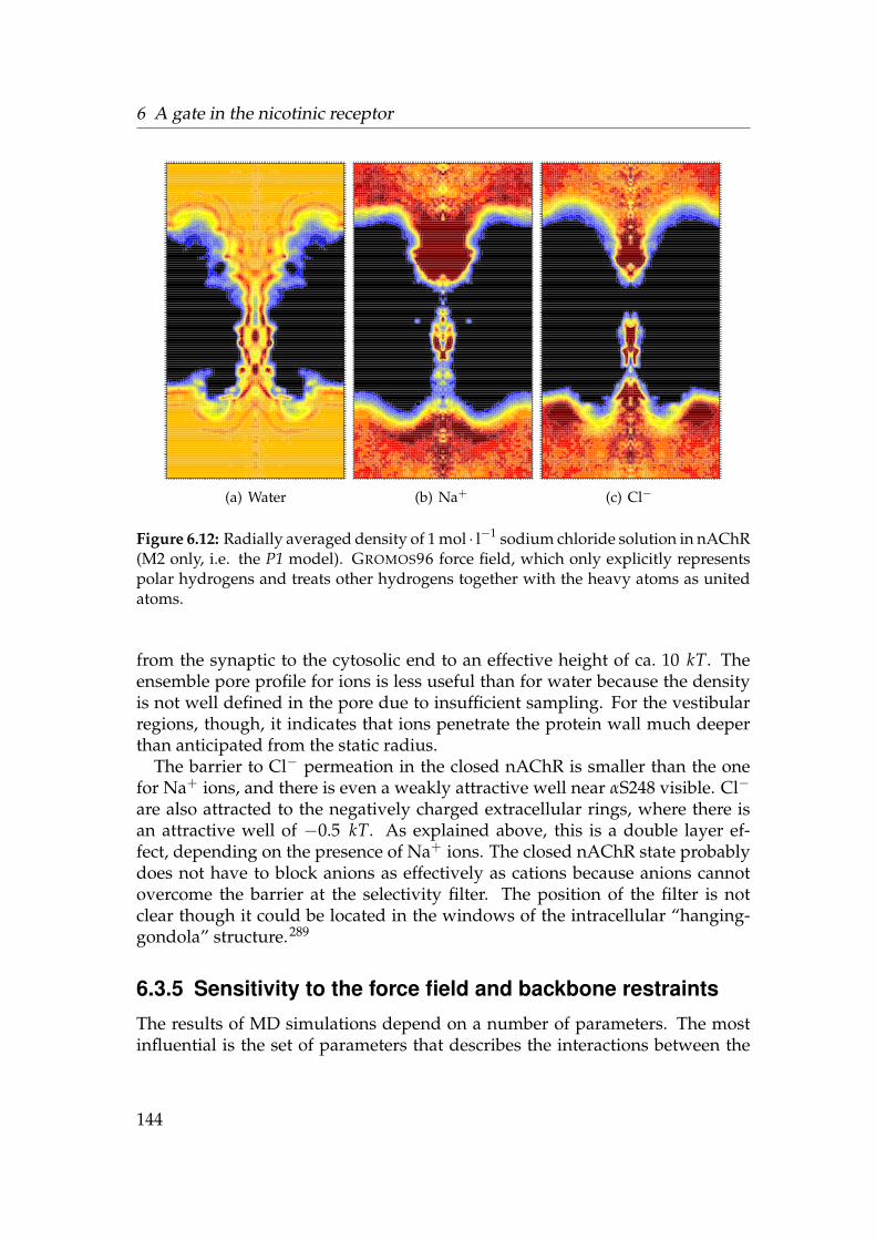
6 A gate in the nicotinic receptor
(a) Water (b) Na+ (c) Cl−
Figure 6.12: Radially averaged density of 1 mol · l−1 sodium chloride solution in nAChR(M2 only, i.e. the P1 model). GROMOS96 force field, which only explicitly representspolar hydrogens and treats other hydrogens together with the heavy atoms as unitedatoms.
from the synaptic to the cytosolic end to an effective height of ca. 10 kT. Theensemble pore profile for ions is less useful than for water because the densityis not well defined in the pore due to insufficient sampling. For the vestibularregions, though, it indicates that ions penetrate the protein wall much deeperthan anticipated from the static radius.
The barrier to Cl− permeation in the closed nAChR is smaller than the onefor Na+ ions, and there is even a weakly attractive well near αS248 visible. Cl−
are also attracted to the negatively charged extracellular rings, where there isan attractive well of −0.5 kT. As explained above, this is a double layer ef-fect, depending on the presence of Na+ ions. The closed nAChR state probablydoes not have to block anions as effectively as cations because anions cannotovercome the barrier at the selectivity filter. The position of the filter is notclear though it could be located in the windows of the intracellular “hanging-gondola” structure.289
6.3.5 Sensitivity to the force field and backbone restraints
The results of MD simulations depend on a number of parameters. The mostinfluential is the set of parameters that describes the interactions between the
144

6.3 Results
V255 V259 L251T244E241 V271S248 E262 S266
-3 -2 -1 0 1 2 3z−zcom [nm]
0
1
2
3
4
5
6
7
n wat
er/n
0an
d n
ion [m
ol/l]
water (LD)waterNa+
Cl−
(a) GROMOS96, SPC water
V255 V259 L251T244E241 V271S248 E262 S266
-3 -2 -1 0 1 2 3z−zcom [nm]
0
1
2
3
4
5
6
7
n wat
er/n
0an
d n
ion [m
ol/l]
water (LD)waterNa+
Cl−
(b) OPLS-AA, TIP4P water
Figure 6.13: Axial density n(z) in nAChR when using alternative force field parameters.See the caption of Fig. 6.9 on page 139.
atoms, i.e. the force field. It contains the parameters for the protein, the watermodel, and the ions. Ideally, all well-tested force fields should give the sameanswer for a given problem. Unfortunately, this is not always the case. PMFs inparticular are known to be sensitive to the force field that is used.298 In order todiscuss the robustness of the results presented in the previous sections, whichwere obtained with the all-atom OPLS-AA force field, we also show simulationscarried out with the united atom GROMOS96 (G43A1) force field. Briefly, someresults for OPLS-AA with the TIP4P water model instead of SPC are also men-tioned. Lastly, the effect of restraining the protein backbone of the M2 helices isdiscussed.
All-atom versus united atom Clear differences between the GROMOS96 andOPLS-AA simulations are already visible in the axial density n(z), Fig. 6.13(a)compared to Fig. 6.9 on page 139. The all-atom simulations do not show anyionic density in the pore but with GROMOS96 high concentrations of both Cl−
(about 3 mol · l−1) and Na+ (2 mol · l−1) are apparent in the cavity near αL251.The simulations started with ions in the pore but whereas they are expelled fromthe pore in the first 0.1 ns of the OPLS-AA simulations they seem to persist oreven exchange in the united-atom simulations. Though the behaviour of waterdoes not seem to differ with resepct to the density it was nevertheless observedby inspection of the trajectories that water (both SPC and TIP4P) with OPLS-AAis much more volatile in the hydrophobic gate region than with GROMOS96.It does exhibit liquid-vapour transitions though not as pronounced as in themodel pores or as in the MscS gate.56 SPC water with GROMOS96, on the other
145

6 A gate in the nicotinic receptor
hand, solvates the pore during the whole simulation time.In both cases, though, the ionic density vanishes at the hydrophobic gate. If
anything, the GROMOS96 density Fig. 6.13(a) shows even clearer the position ofthe gate.
The higher density in the cavity region in GROMOS96 simulations does not ap-pear to be an artifact of initial conditions. The Na+ PMF exhibit a correspondingdouble peak structure with an attractive valley in the cavity (Fig. 6.14(b)). Thebarrier at the hydrophobic gate (7.2 kT) is about the same height as the secondbarrier between αT244 and αS248 with 6.8 kT (within estimated errors of 1 kT);both barriers are lower than the Na+ barrier in OPLS-AA with 8.7 kT. The Cl−
barrier, Fig. 6.14(c), has one pronounced peak at the same location at αV255 asin the OPLS-AA simulations, but it is higher with 8.5 kT compared to 7 kT, andit lacks the attractive well near αS248.
Water model and ionic strength The use of the TIP4P model with OPLS-AAinstead of SPC did not lead to dramatic changes in the density, as can be seenby comparing n(z) (Fig. 6.13(b) with Fig. 6.9 on page 139) or the radial densityn(r, z) (Fig. 6.12(a) with Fig. 6.8(a) on page 138). This was taken as an indicationthat the PMF would probably not differ very much from the SPC/OPLS-AA case.
For the GROMOS96 case we also assessed the effect of the presence of ions onthe water PMF. In Fig. 6.14(a) the equilibrium density derived PMF of water in1.3 mol · l−1 NaCl is compared to the PMF of a water molecule in pure water.The difference is barely noticeable, which suggests that the influence of ions onwater structure in the pore is actually very small.
Backbone restraints In Section 6.2.2 it was described how the full TM do-main of nAChR was reduced to the P1 model. In order to retain the experi-mental structure, the backbone atoms of the M2 helices were harmonicly re-strained with force constant kbb = k0, which could be a source for artifacts inthe PMF. To assess the influence of the restraints we also computed one PMF fora Na+ ion at much weaker restraints kbb = 0.2k0. Both PMFs are very similar(Fig. 6.15), and within an estimated error of 1 kT indistinguishable. We believe
Figure 6.14: PMF of water and ions in the nAChR pore at a bulk NaCl concentrationof about 1.3 mol · l−1. MD simulations and umbrella sampling were performed withthe GROMOS96 force field. The equilibrium derived PMF is shown as a dashed lineand the Umbrella sampled PMF as a heavy line. For water (a), there is also shown theequilibrium density for nAChR solvated in pure water (dotted line). The pore radius(from hole) is shown below, together with the ensemble pore radius. Important porelining residues (on the α subunit) are indicated.
146

6.3 Results
V255 V259 L251T244E241 V271S248
0
0.5
1
R [
nm] -3 -2 -1 0 1 2 3
z−zcom [nm]
0
2βG
(z)
(a) Water
V255 V259 L251T244E241 V271S248
0
0.5
1
R [
nm] -3 -2 -1 0 1 2 3
z−zcom [nm]
-2
0
2
4
6
8
βG(z
)
(b) Na+
V255 V259 L251T244E241 V271S248
0
0.5
1
R [
nm] -3 -2 -1 0 1 2 3
z−zcom [nm]
-2
0
2
4
6
8
10
βG(z
)
(c) Cl−
147
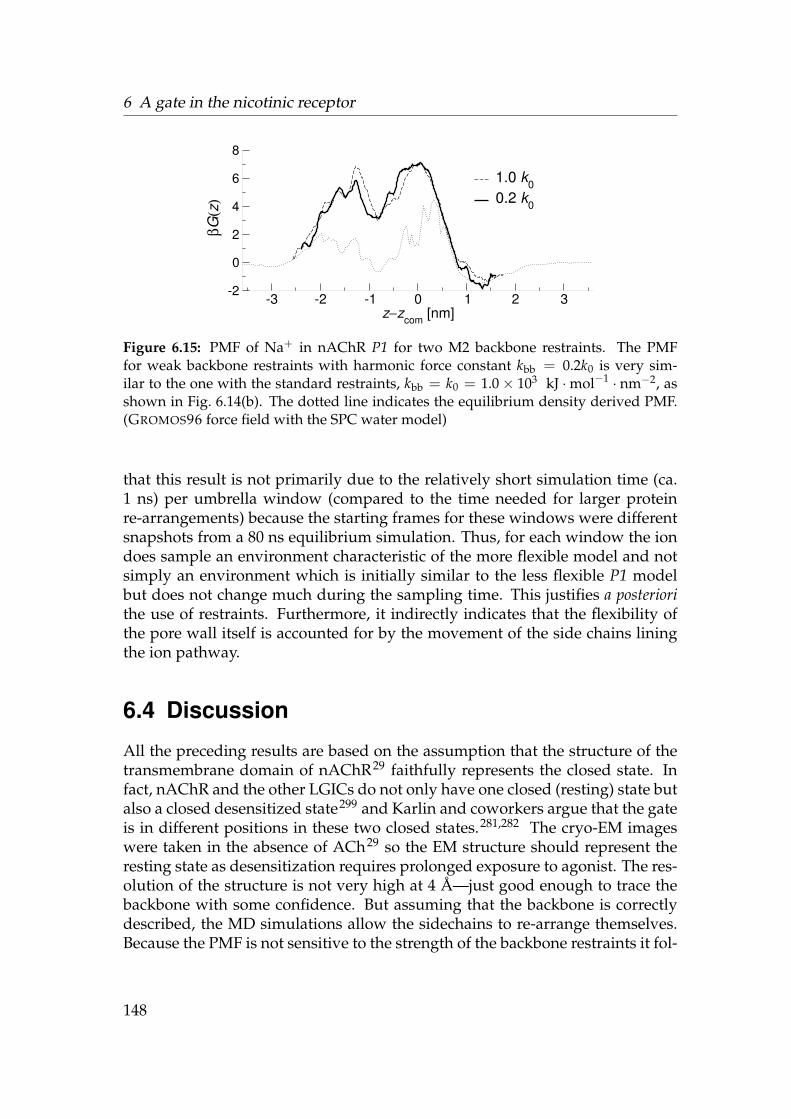
6 A gate in the nicotinic receptor
-3 -2 -1 0 1 2 3z−zcom [nm]
-2
0
2
4
6
8
βG(z
)
1.0 k00.2 k0
Figure 6.15: PMF of Na+ in nAChR P1 for two M2 backbone restraints. The PMFfor weak backbone restraints with harmonic force constant kbb = 0.2k0 is very sim-ilar to the one with the standard restraints, kbb = k0 = 1.0× 10³ kJ ·mol−1 · nm−2, asshown in Fig. 6.14(b). The dotted line indicates the equilibrium density derived PMF.(GROMOS96 force field with the SPC water model)
that this result is not primarily due to the relatively short simulation time (ca.1 ns) per umbrella window (compared to the time needed for larger proteinre-arrangements) because the starting frames for these windows were differentsnapshots from a 80 ns equilibrium simulation. Thus, for each window the iondoes sample an environment characteristic of the more flexible model and notsimply an environment which is initially similar to the less flexible P1 modelbut does not change much during the sampling time. This justifies a posteriorithe use of restraints. Furthermore, it indirectly indicates that the flexibility ofthe pore wall itself is accounted for by the movement of the side chains liningthe ion pathway.
6.4 Discussion
All the preceding results are based on the assumption that the structure of thetransmembrane domain of nAChR29 faithfully represents the closed state. Infact, nAChR and the other LGICs do not only have one closed (resting) state butalso a closed desensitized state299 and Karlin and coworkers argue that the gateis in different positions in these two closed states.281,282 The cryo-EM imageswere taken in the absence of ACh29 so the EM structure should represent theresting state as desensitization requires prolonged exposure to agonist. The res-olution of the structure is not very high at 4 A—just good enough to trace thebackbone with some confidence. But assuming that the backbone is correctlydescribed, the MD simulations allow the sidechains to re-arrange themselves.Because the PMF is not sensitive to the strength of the backbone restraints it fol-
148

6.4 Discussion
V13’ V17’L9’T2’E-2’ V29’S6’ E20’ S24’
V255 V259 L255T244αE241 V271S248 E262 S266-0.5
0
0.5
R [n
m] -3 -2 -1 0 1 2 3
z−zcom [nm]-2
0
2
4
6
8
10PM
F β
G(z
) Na+
Cl−water
Figure 6.16: Potential of mean force of ions and water in nAChR. Na+ ions encountera wide barrier of up to 8.7 kT, which is peaked at the hydrophobic girdle (L9′–V13′)—the hydrophobic gate (marked in yellow). The barrier for Cl− is somewhat lower whichimplies that the anion filter is located in other parts of the permeation pathway. Watersolvates the pore because the barrier is not greater than 2 kT. The pore profile is shownin the lower panel, mirrored at the axis to create the impression of a section through thenAChR pore.
lows that the local pore environment, which is formed by the mobile sidechains,assumes a conformation independent of the details of the backbone motions. Itappears that molecular dynamics fills in the functional details which could notbe resolved through experiment.
The Na+ PMF (Fig. 6.16) shows a pronounced barrier of about 8.7 kT at thehydrophobic girdle (between αL251 = 9′ and αV255 = 13′). Therefore, thehydrophobic girdle is identified with the hydrophobic gate of nAChR, as hypo-thesised by Unwin and colleagues,29,61 who based their inference on the pro-tein structure. This finding disagrees with the results of Karlin and cowork-ers275,281,282 who predict the position of the (resting) gate at about αT244 = 2′,based on biochemical data (accessibility of substituted cysteines to small, posit-ively charged, sulfhydryl-specific reagents). However, using the same methodin the closely related 5HT3A receptor, Slesinger et al.286 find evidence for a gatebetween residues 9′ and 13′, and further experiments indicate that the narrow
149
6 A gate in the nicotinic receptor
constriction site near 2′ remains unchanged between the open and the closedstate287—the very same region that Karlin275,281,282 identifies as the gate. A gateat the position of the hydrophobic girdle is also consistent with experimentalresults by Auerbach and colleagues who describe gating in nAChR as a waveof conformational change284 propagating from the ligand binding domain tothe middle of the M2 segment, hence implying a gate near 9′.285 Based on func-tional and behavioural studies of mutations in the muscle283 (α2βγδ) and brain(α4β2) nAChR300,301 of mice, Lester and coworkers attribute a central role ingating to Leu9′. A Leu to Ser mutation in the α4 receptor confers hypersensit-ivity to ACh and constant activation, leading to behavioural abnormalities andpostnatal lethality in knock-in mice.300 A less severe Leu to Ala mutation leadsto a 50-fold increase in sensitivity to nicotine.301 Mice bearing the mutation areotherwise healthy (in contrast to the Leu9′Ser mice). Not only do these gain-of-function experiments hint at an explanation of nicotine addiction (the α4β2nAChR, which is part of the dopaminergic reward system in the brain, is neces-sary and sufficient in mice for the behavioural effects of nicotine to be elicited)but also suggests that an increase in hydrophilicity in the gate region will lead toa greater likelihood of channel openings. This can be interpreted as a decreasein the barrier to ion permeation, which decreases with an increase in polarity(Ser, and to a lesser degree Ala) or with an increase in pore radius (Ala), whichin turn provides more space for hydrating water molecules.
The question remains if the calculated barrier (∆G‡ = 22 kJ ·mol−1 = 8.7 kTat T = 300 K) is actually large enough to prevent passage of ions. Allen et al.170
computed K+ PMFs in the gramicidin A channel and determined a barrier of34 kJ ·mol−1 (12.4 kT at the temperature of the simulation, T = 330 K). Theycalculate a maximum conductance gmax = 0.8 pS for the open channel.∗ We usetheir Eq. 5 (see also Eq. 18 in Ref. 169),
gmax =e2
kTDeff
L2
=βe2
L2
(L−1
∫P
dz D(z)−1e+βG(z))−1 (
L−1∫P
dz e−βG(z))−1
, (6.1)
to estimate the maximum conductance of the closed nAChR pore. The spatialaverages are carried out over the pore region P (from αE241 to αV271, L =4.5 nm) with the Na+ PMF G(z) (Fig. 6.11(b)). The diffusion constant in theregions where the barrier is small (G(z) < 1 kT) is taken as the experimentalvalue of Na+ at room temperature, D(z) = D0 = 1.33 nm2 · ns−1 (Ref. 12). ForG(z) > 1 kT (in the barrier region) we choose it to be a fraction α of D0, D(z) =
∗The experimental conductance for gA is 21 pS but Allen et al.170 go to considerable lengthto demonstrate that their first-principles gmax of 0.8 pS should be considered a good estimate,an order of magnitude better than any previous ones.
150
6.5 Conclusions
αD0. With a typical value of α = 0.5,95 we obtain gmax = 0.09 pS, which is belowthe detection limit of current patch clamp single channel recordings.∗ At firstglance it might seem surprising that although the maximum barrier height innAChR (8.7 kT) is lower than in gA (12.4 kT), gmax is larger for open gA than forclosed nAChR (0.8 pS and 0.09 pS). The difference lies in the shape and spatialextension of the PMFs. In gA, it is peaked at the centre and the region whereG(z) > 1 kT extends over a length of only about L = 1 nm (Ref. 170, Fig. 2).The nAChR PMF (Fig. 6.11(b)) is much broader and extends over 2.7 nm whichtranslates into a low conductance in Eq. (6.1). gmax is completely dominatedby the average
⟨D(z)−1 exp
(+ βG(z)
)⟩, which in turn is determined by the
region where the barrier is high. Because the barrier is large in the whole poreregion this implies that our estimate gmax directly scales with the fraction ofthe diffusion constant, α. Even if we took α = 2, i.e. diffusion were enhancedin the pore, the corresponding maximum conductance 0.18 pS would still bebelow the experimental noise limit. The rough estimate of the single channelconductance seems to indicate that the nAChR pore, as described by the Na+
PMF, is indeed closed, especially when compared to the open state conductanceof about 30 pS.12
For Cl− the estimated maximum single channel conductance is gmax = 2.9 pS(using D0 = 2.03 nm2 · ns−1 (Ref. 12))—which shows that the barrier for chlor-ide permeation is significantly lower than the one for sodium ions. However,the closed state should not allow the passage of either cations or anions. Be-cause the preceding calculation shows that the closed state nAChR does notefficiently block Cl− flow one must conclude that there exists another region inthe receptor—the selectivity filter—which prevents permeation of Cl−. This se-lectivity filter should be functional both in the closed and the open state of thechannel. The most likely region for the filter are the charge-decorated windowsin the intracellular vestibule.289
6.5 Conclusions
We tried to answer the question where the gate is located in the nicotinic re-ceptor, i.e. we sought to identify the functional region which prevents ions frompermeating the closed channel. We approached the question on the basis of theclosed state cryo electron microscopy structure of Miyazawa et al.29
A direct computational method to find permeation barriers is to calculate thepotential of mean force from fully atomistic molecular dynamics simulations,which, however, require significant computing resources. In order to make
∗At a typical transmembrane voltage of V = 100 mV, a conductance of g ≈ 0.1 pS wouldallow a current I = gV = 0.01 pA to flow (assuming ohmic behaviour). This is below 0.06 pA,the noise limit for current patch clamp experiments.12
151

6 A gate in the nicotinic receptor
the system tractable and achieve sufficient sampling we reduced the systemsize to the bare minimum. We argued that the bare minimum consists of onlythe conduction pathway lining M2 helices (with the backbone atoms harmon-icly restrained to their experimentally determined position) and demonstratedthe negligible influence of the outer helices on the (electrostatic) PMF. The lig-and binding domain, which was not modelled in the PMF calculations, wouldprobably increase the height of the barrier because it extends the low dielec-tric region in the vicinity of the pore, but more work is required to address thisquestion. The cytosolic vestibule, the structure of which is not known at atomicresolution, has the shape of a sphere with inner radius of about 1 nm.265 Inthe absence of any structure we can speculate that its main influence on ionpermeation in the transmembrane domain would be similar to the one of theligand binding domain, i.e. it would raise the existing barriers. Its particularshape and charge decoration might very well contribute significantly to overallconductance and selectivity.289
The Na+ PMF shows a pronounced barrier of about 8.7 kT or 22 kJ ·mol−1 atthe hydrophobic girdle (αV255). In the absence of any other barriers, which, weargued, can only be located in the TM pore itself, this identifies the hydrophobicgirdle with the hydrophobic gate of nAChR, consistent with structural29,58 andmost283–287 but not all281,282 biochemical evidence. The simulation results donot support the notion of a gate close to the intracellular mouth. Additionalsupport for the plausibility of the PMF comes from a rough estimate for thesingle channel conductance of about 0.1 pS, which is very small compared tothe experimental open state conductance of about 30 pS (Ref. 12) and below thedetection limit of patch clamp recordings.
As a secondary result we established the function of the extracellular doublering and the intermediate/intracellular rings as concentrators of cations. Byincreasing the local ion concentration near the channel entrance, the proteinlowers the effective access resistance and thus can increase the single-channelcurrent once it opens.12 Furthermore, the nAChR pore was shown to be pre-dominantly filled with water in the closed state.
The shape of the PMF was found to be somewhat sensitive to the force field.We presented results for the all atom OPLS-AA force field because it is thoughtto better represent the pore environment. The results are also more in linewith what one would expect from the studies on the simple hydrophobic pores,namely that for a given radius the hydrophobic region should be responsible fora higher permeation barrier than the polar one. Nevertheless, both force fieldsdo exhibit a significant barrier at the hydrophobic girdle, which reinforces themain finding of this chapter: That there is a hydrophobic gate in the nicotinicreceptor, and that we can understand its existence on the grounds of simpleconcepts.
152
7 Conclusions
Structural evidence suggests that the gate in many ion channels is formed by ahydrophobic constriction of the pore; for the known ion channels this appearsto be the predominant form of the gate (the other being a block by a single side-chain). In the closed-state nicotinic receptor this constriction is wide enough tolet three water molecules or a half-solvated sodium ion pass. The hydrophobiccharacter of the sidechains lining the constriction appears to be responsible forthe barrier to ion permeation and hence this was termed a hydrophobic gatingmechanism. So far, evidence in the literature only consisted of static structureimages29,48,59,66 and the qualitative reasoning that the loss of the hydration shellof an ion would be energetically so costly as to prevent the ion from permeat-ing.12,67
In this work only hydrophobic gating was considered; other authors havedealt with gates formed by local sidechains in the context of the chloride chan-nels31,302–307 and an outer membrane protein.39 “Local gating” differs from hy-drophobic gating in that only small structural rearrangements are required toopen the gate, and the details of the local environment (the gating sidechainitself and local networks of hydrogen bonds and salt bridges) are crucial toexplain the mechanism. Furthermore, permeating ions or protons themselvesmight be involved in the gating process. On the other hand, hydrophobic gatinginvolves large scale movements of the protein to open the gate. The commonfeature of hydrophobic gates is a ring of hydrophobic residues but the exactcomposition is variable. This suggests that there is a common mechanism atwork, a general principle, which has evolved in a wide range of systems. In thiswork an attempt was made to identify this mechanism, explain it, and quantifyit, with the help of computational methods.
7.1 Water: Capillary effects at the atomic scale
In understanding ion permeation it is also necessary to understand the beha-viour of the solvent, i.e. water. Water is not a simple liquid due to its strong hy-drogen bonds (which, for instance, leads to the hydrophobic effect), and understandard condition it is also a liquid close to its liquid-vapour phase transition.In Chapter 3 and Chapter 4 water was studied confined to narrow hydrophobicpores of the dimensions of the gate of the nicotinic acetylcholine receptor. Theradius of these pores ranged from the radius of a water molecule to seven times
153

7 Conclusions
as much. These model pores were kept conceptually and structurally simplein order to minimise the number of free parameters and so to be able to disen-tangle different contributions to a gating effect.
The water density in the pore did not gradually decrease with radius buttwo distinct states were found: The water was either liquid, comparable to bulkwater, or it formed a vapour, but no intermediate state existed. Macroscopically,the phenomenon of capillary evaporation and condensation is well known forfluids confined to a pore. In this situation the interface between fluid and wallplays a more important role compared to volume properties. For a fluid close toa phase transition the interaction between the fluid molecules and the wall candrive the fluid across the phase transition. The observed oscillations betweenliquid water and water vapour in the microscopic pores could be explained ascapillary evaporation/condensation, driven by thermal density fluctuations inthe water outside the pore itself. Through a thermodynamic model the strengthof the effect was related to the hydrophobicity of the surface, expressed as thecontact angle or equivalently, the wall-water surface tension.
The simple model pores allowed to investigate different parameters that af-fected water transport, namely the geometry of the pore (radius and length), thechemical character of the surface (hydrophobic vs. hydrophilic), and the flexib-ility of the pore wall. Liquid water was forced out of pores with smaller radii,more hydrophobic and more flexible pore walls. Conversely, liquid water wasstabilised in wide pores with hydrophilic and rigid pore walls. For the short(length 0.8 nm) hydrophobic pores studied here, the critical or transition radiusbetween the vapour and the liquid regime was at about 0.56 nm while the wallatom position fluctuated by about 0.072 nm.
At least theoretically, this demonstrates that capillarity effects are present inatomic scale systems, such as fluid transporting conduits in nanotechnology,geology (water transport in rocks such as zeolites), and in biological proteinchannels. It seems that in the case of hydrophobic cavities natura non abhorretvacuum—or at least is content with filling it with the occasional vapour or gasmolecule instead of with the surrounding water.
7.2 Ions: Dehydration barriers
Equilibrium molecular dynamics simulations of Na+ and Cl− ions in the modelpores (Chapter 4) showed that ions would not permeate hydrophobic pores ofradius less than about 0.6 nm over time-scales of about 100 ns, indicating thatthe hydrophobic constriction represents a high free energy barrier to ion per-meation. This barrier was explicitly probed by calculating the potential of meanforce for ion permeation from biased simulations (Chapter 5). For a pore of ra-dius 0.3 nm, the barrier height measures almost 20 kT (or about 50 kJ ·mol−1),
154
7.3 A hydrophobic gate in the nicotinic receptor
which renders the pore impermeable to ions having an average thermal en-ergy of about 1 kT. Insight into the origin of this barrier comes from Poisson-Boltzmann calculations of the same system, in which the water is only treatedas a high-dielectric continuum but which incorporate all electrostatic effects.For very narrow pores (up to twice the water radius) the barrier originates inthe high electrostatic energy to place a bare charged particle at the centre of alow dielectric membrane (the Born barrier); because the pore is narrow, there isno space for water molecules to solvate the ion and hence the barrier becomescomparable in magnitude to the cost to completely dehydrate the ion. For widerpores the barrier is much higher than predicted on electrostatic grounds aloneeven though there would be room for almost one complete hydration shellaround the ion. The reason is that water itself is not stable in the pore and has atendency to evaporate from the pore due to the hydrophobic nature of the wall.This explains how hydrophobic pores as wide as 1 nm in diameter (and only0.8 nm in length) can effectively be impermeable to ions. Hence, a hydrophobicpore need not be sterically occluded to act as an barrier to ion permeation.
The computational approach presented here provides strong evidence for ageneral hydrophobic gating mechanism. Major factors influencing the barrierto ion permeation are the chemical character of the pore wall, its radius, andalso its flexibility or rigidity.
7.3 A hydrophobic gate in the nicotinic receptor
The model pores were designed as radically simplified versions of the nicotinicreceptor gate. They were also more hydrophobic than any real protein. Eventhough hydrophobic sidechains present a surface similar to the methyl termin-ated surface of the model pores there is always at least the peptide bond dipolepresent so that the specific protein environment might mask or perhaps evennullify the hydrophobic gating effect. Hence, in Chapter 6 simulations were car-ried out to find the position of the gate in the closed-state nAChR pore, whichcontains a pronounced hydrophobic girdle with a pore radius of R = 0.31 nmbut is generally much more complex than the model pores. Free energy cal-culations of the potential of mean force revealed a barrier to Na+ permeation,peaked at the hydrophobic girdle formed at αL251 = L9′ and αV255 = V13′ witha height of 8.7 kT and extending over a length of more than 2 nm—almost thewidth of the membrane. Estimates of the single channel conductance are belowthe detection limit of experimental single channel recordings, which suggeststhat the hydrophobically sealed pore could function as a closed gate.
The calculations directly relate the structure of the nAChR channel to a func-tional characteristic. The observed gate can be rationalised on the basis ofthe calculations of the preceding chapters as a desolvation barrier to ion per-
155
7 Conclusions
meation, created by a hydrophobic constriction, i.e. a cylindrical pore with ahigh surface tension wall. Because the underlying principle should be gener-ally applicable in a wider context and not just in the particular case of nAChRit is expected to play a role in other ion channels as well.
7.4 Confinement effects in other systems
The principles laid out in the present work have already been applied by otherauthors in a variety of biological systems. A brief outline of these authors’ find-ings is presented here with reference to the results of the preceding chapters.
A gate in MscS The nicotinic receptor is not the only ion channel whose struc-ture features a wide hydrophobic pore. The bacterial mechanosensitive channelof small conductance MscS displays a wide R = 0.32 nm hydrophobic con-striction; on this ground it was originally believed to be captured in the openstate.55 Molecular dynamics simulations by Anishkin and Sukharev56, how-ever, showed that water evaporated from the MscS gate in the same way asseen in the hydrophobic model pores in Chapter 3. The authors termed thisa “vapour-lock” mechanism, explicitly referring to results presented here.62,96
Their work, together with the results for the muscle-type nAChR (Chapter 6)and the related α7 receptor (Appendix A), allows the tentative conclusion thathydrophobic gating is not dependent on a particular local protein environmentbut only relies on broad features, namely a non-polar constriction not muchwider than 0.6 nm in diameter and about two α-helical turns in length.
Water transport through KcsA Liquid-vapour oscillations96 were also in-voked by Saparov and Pohl308 to explain how the potassium channel KcsA canconduct water 100 times faster than the specialised water channel Aqp1. Waterflux measurements under conditions of low K+ concentrations (< 0.2 mol · l−1)yielded a very large water flux of 1.6× 10² ns−1. This flux could be gated bypH in the same way as the ionic flux is gated (KcsA opens below pH 4). Thehigh turnover rate for water is—in the absence of K+ in solution—independentof the osmotic driving force, i.e. an “all-or-none mechanism.” Furthermore, ad-dition of K+ at concentrations greater than 0.2 mol · l−1 limits water transportto the turnover rate of the ions (< 0.1 ns−1); for each ion, two water mole-cules are dragged along. The turnover rate changes from fast water transportto slow (ion limited) transport over a very small K+-concentration range (atca. 0.2± 0.01 mol · l−1) in a step-like fashion. Even though the interior of KcsAis not especially hydrophobic, Saparov and Pohl308 suggest that the observed
156
7.4 Confinement effects in other systems
behaviour can be explained by capillary evaporation in the absence of K+ in thechannel and subsequent fast water transport in the vapour phase.
The amphipathic carbamate tunnel Kim and Raushel309 discuss the signific-ance of the surface character of the tunnel in the enzyme carbamoyl phosphatesynthetase (CPS). A largely hydrophobic tunnel of length 10 nm connects threeactive sites, which catalyse the hydrolysis of glutamine to ammonia, and phos-phorylation of bicarbonate and carbamate respectively. The reactive carbamateion NH2COO− diffuses through the second half of the tunnel over ca. 5 nm.Five conserved glutamates with four bound water molecules provide hydro-philic patches in the tunnel. At least some of the glutamates are suspected to bein their protonated (uncharged) state as the hydrophobic environment wouldshift the local Glu pKa to higher values, favouring protonation. Physiologicallythis is required because the intermediate carbamate needs to be protected fromprotonation (it is unstable at low pH ) so the glutamate residues probably actas proton scavengers. Two arginines at either end control access to the tunnel;mutation to alanine also disrupts substantially the ability of CPS to catalyse thesynthesis of carbamoyl phosphate. The authors interpret their findings in thelight of the MD simulations of water in hydrophobic pores,62 which were madeincreasingly hydrophilic through the addition of dipoles. They conclude thatthe carbamate tunnel contains a finely tuned set of polar residues in an overallhydrophobic environment which “opens” an otherwise “closed” hydrophobictunnel.309 The conserved Arg residues fulfil the role of gate-keepers, which steerthe carbamate ion into or out of the tunnel.
“Are sobriety and consciousness determined by water in proteincavities?”22 Ethanol (and butanol) are believed to produce their sedative-hypnotic effects in mammals by directly affecting ligand gated ion channels.310
Alcohols are thought to bind in cavities which are normally water filled. Trudelland Harris22 suggest that alcohols can only compete with cavity-water for bind-ing because the enclosed water is—due to confinement—poised for evapora-tion.96 That is, neurological states ultimately depend on the stability of liquidphase water in ion channels. Furthermore, it was shown that moderate in-creases in pressure (to 12 atmospheres) act as an antagonist to alcohols, revers-ing the effect of ethanol and butanol on GABAA and glycine α1 receptors, twoion channels of the central nervous system.311,312 This result seems to be con-sistent with a view that increased external pressure stabilises liquid water ina cavity (or pore), as expressed in the Kelvin equation or Eq. (4.5). Quantitat-ively, an increase in pressure by 12 bar does not seem to be sufficient to changethe equilibrium between liquid and vapour (the magnitude of the effect is only
157

7 Conclusions
about one tenth of the surface tensions involved).∗ However, the simulations ofthe nicotinic receptor showed that the particular protein environment can leadto some deviations from the ideal hydrophobic model pore behaviour, so it can-not be ruled out that pressure effects play a greater role in the case of watercavities in ligand gated ion channels.
7.5 Function follows from form
The American architect Louis Sullivan (1856–1924)313 expressed the principlethat design should follow from the purpose of the object:
Whether it be the sweeping eagle in his flight, or the open apple-blossom, the toiling work-horse, the blithe swan, the branching oak,the winding stream at its base, the drifting clouds, over all the cours-ing sun, form ever follows function, and this is the law. Where functiondoes not change form does not change.314
He intuitively recognised the principle that evolution shapes living organisms,and that their form expresses adaptation to a particular niche—from whole or-ganisms down to the molecules that they are made from. He saw beauty in thisconcept and advocated an approach to design which is embodied in the phraseform follows function.
One of the fundamental aims of structural biology is to explain protein func-tion based on protein structure. The hydrophobic gating effect, which was dis-cussed in this work, is one example for such an explanation. It helps us tounderstand the position and the function of gates in a range of ion channelstructures, i.e. we infer function from the structure, or—applying the inverse ofSullivan’s principle—the function follows from the form.
∗MD simulations of water in hydrophobic model pores at p = 12 bar did show a small butprobably not significant shift towards the liquid state, with the main effect being a more rapidfilling transition (data not shown).
158

Appendices
159


A The α7 receptor
The α7 receptor is a homopentameric neuronal nicotinic acetylcholine re-ceptor.25 Amiri et al.41 constructed a model of the full receptor from homologymodels of its separate domains, based on the Gallus gallus (chick) sequence.∗
The transmembrane (TM) domain was modelled on the TM domain of the Tor-pedo marmorata muscle-type nAChR29 (4 A resolution) whereas the 2.7 A struc-ture of Lymnea stagnalis (snail) acetylcholine binding protein279 (AChBP) wasused for the ligand binding (LB) domain. The two domains were fused by analignment procedure that accounts for stereochemical clashes, continuity of theamino acid chain, and closeness of functionally important residues.41 The fullmodel (Fig. A.1) exhibits a wide, aqueous pore in the LB domain. The TM poreresembles the one of muscle nAChR though some details are different. Mostnotably, the constriction at the 6′ position (R = 0.2 nm) is narrower in α7 thanin Torpedo nAChR (R = 0.3 nm; compare the pore profiles in Fig. A.2 to Fig. 6.11on page 142).
Further details can be found in Amiri et al.41; in the following only the PMFcalculations for a Na+ ion in the α7 receptor are described.
A.1 Methods
Born energy calculations were performed as described in Section 6.2.3 at a con-centration of 1 mol · l−1 NaCl. The bounding box for the whole receptor meas-ured 9.6 nm× 9.6 nm× 21.0 nm and is considerably larger than the one usedfor Torpedo nAChR TM. In order to obtain a reasonable resolution, a grid ofdimensions 97 × 97 × 193 cells was employed and focused into a volume of1 nm× 1 nm× 1 nm, centred on the test ion. Electrostatic PMFs were calculatedboth for the full model (LB and TM domain) and the M2 bundle on its own(always embedded in a membrane mimetic slab); the same box size and griddimensions were used in both cases.
Umbrella sampling of a Na+ ion and 60 ns equilibrium molecular dynamics(MD) on the M2 helices of the chick α7 receptor model were carried out withthe GROMOS96 (G43A1) force field and the SPC water model at a nominal con-centration of 1 mol · l−1 NaCl. All other parameters are identical to the PMF
∗The intracellular basket is missing from the “full” model because no atomic resolutionstructural data are available.
161
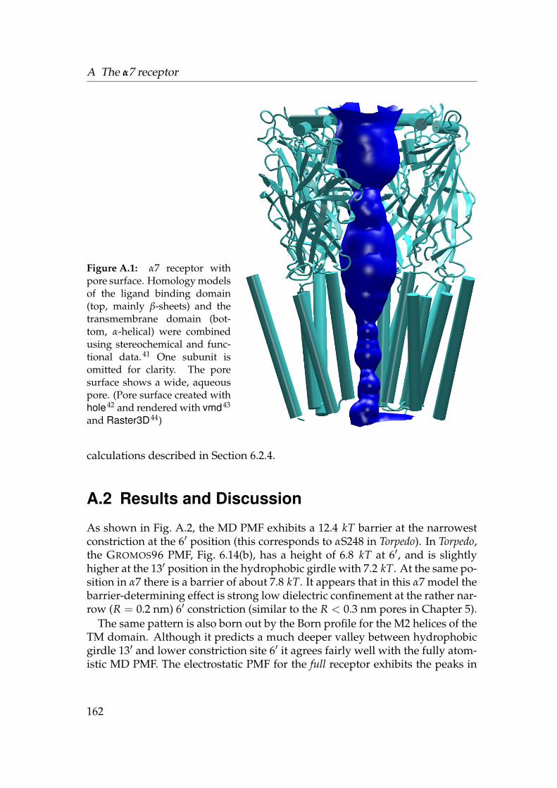
A The α7 receptor
Figure A.1: α7 receptor withpore surface. Homology modelsof the ligand binding domain(top, mainly β-sheets) and thetransmembrane domain (bot-tom, α-helical) were combinedusing stereochemical and func-tional data.41 One subunit isomitted for clarity. The poresurface shows a wide, aqueouspore. (Pore surface created withhole42 and rendered with vmd43
and Raster3D44)
calculations described in Section 6.2.4.
A.2 Results and Discussion
As shown in Fig. A.2, the MD PMF exhibits a 12.4 kT barrier at the narrowestconstriction at the 6′ position (this corresponds to αS248 in Torpedo). In Torpedo,the GROMOS96 PMF, Fig. 6.14(b), has a height of 6.8 kT at 6′, and is slightlyhigher at the 13′ position in the hydrophobic girdle with 7.2 kT. At the same po-sition in α7 there is a barrier of about 7.8 kT. It appears that in this α7 model thebarrier-determining effect is strong low dielectric confinement at the rather nar-row (R = 0.2 nm) 6′ constriction (similar to the R < 0.3 nm pores in Chapter 5).
The same pattern is also born out by the Born profile for the M2 helices of theTM domain. Although it predicts a much deeper valley between hydrophobicgirdle 13′ and lower constriction site 6′ it agrees fairly well with the fully atom-istic MD PMF. The electrostatic PMF for the full receptor exhibits the peaks in
162
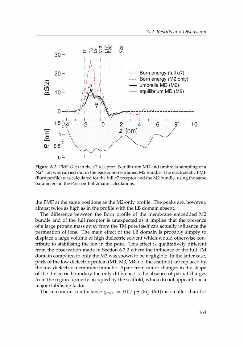
A.2 Results and Discussion
I1’
T6’
L9’
V13
’L1
7’E
20’
V29
’
0
0.5
1
1.5
R [
nm]
-4 -2 0 2 4 6 8 10z [nm]
0
10
20
30βG
(z)
Born energy (full α7)Born energy (M2 only)umbrella MD (M2)equilibrium MD (M2)
Figure A.2: PMF G(z) in the α7 receptor. Equilibrium MD and umbrella sampling of aNa+ ion was carried out in the backbone-restrained M2 bundle. The electrostatic PMF(Born profile) was calculated for the full α7 receptor and the M2 bundle, using the sameparameters in the Poisson-Boltzmann calculations.
the PMF at the same positions as the M2-only profile. The peaks are, however,almost twice as high as in the profile with the LB domain absent.
The difference between the Born profile of the membrane embedded M2bundle and of the full receptor is unexpected as it implies that the presenceof a large protein mass away from the TM pore itself can actually influence thepermeation of ions. The main effect of the LB domain is probably simply todisplace a large volume of high dielectric solvent which would otherwise con-tribute to stabilising the ion in the pore. This effect is qualitatively differentfrom the observation made in Section 6.3.2 where the influence of the full TMdomain compared to only the M2 was shown to be negligible. In the latter case,parts of the low dielectric protein (M1, M3, M4, i.e. the scaffold) are replaced bythe low dielectric membrane mimetic. Apart from minor changes in the shapeof the dielectric boundary the only difference is the absence of partial chargesfrom the region formerly occupied by the scaffold, which do not appear to be amajor stabilising factor.
The maximum conductance gmax = 0.02 pS (Eq. (6.1)) is smaller than for
163
A The α7 receptor
Torpedo nAChR (0.1 pS, see Section 6.4), which is expected due to the largerbarrier. It also indicates that the α7 receptor models a closed state.
It should be noted that the PMF and hence gmax depends rather sensitivelyon the geometry. Narrow constrictions will show up as large barriers in thePMF. These narrow constrictions might be a result of the homology modellingprocedure, which are then frozen-in by the backbone restraints in the MD. Itis possible that after extended free MD the pore opens up which in turn couldlead to a geometry more similar to the Torpedo nAChR.
A.3 Conclusions
Preliminary calculations of the molecular dynamics and electrostatic PMF ina model of the α7 nicotinic acetylcholine receptor have been performed. Whenthe electrostatic calculations are performed on the same reduced receptor model(M2 bundle) then both PMFs agree reasonably well, in contrast to the caseof the model pores in Section 5.3.1. Either the agreement is fortuitous or thePoisson-Boltzmann calculation perform better in a system where there is moreelectrostatic influence than just the dielectric barrier. The Born profile for thetransmembrane region and the extracellular ligand binding domain, however,is dominated by barriers almost twice as high as in the TM-only profile. Moreextensive (and much more costly in required computing resources) MD um-brella sampling calculations would need to be carried out to verify this effect.If shown to be true then it would have interesting implications on ion channelpermeation. In particular, voluminous “protein-appendices” like the intracellu-lar basket of the ligand gated ion channels could also function as attenuators ofconductance, simply by their far reaching electrostatic influence.
Acknowledgements The α7 model was kindly provided by Shiva Amiri. TheBorn profile on the full receptor was calculated by Kaihsu Tai.
164

B A consistent definition of volume at themolecular scale
B.1 Introduction
The correct description of atomic scale phenomena is based on statistical mech-anics and quantum mechanics. Nevertheless, classical descriptions of the in-teratomic forces, which parameterize the interatomic potentials as two, three,or four-body interactions, have been fairly successful.
It even appears that macroscopical concepts like surface tension can be ap-plied down to the molecular scale.113,254 This concept is employed in manyempirical docking programs where the “hydrophobicity” of a sidechain is ef-fectively parameterized as a surface tension times accessible surface area. Onceone applies macroscopical concepts at the molecular scale one realises that somewell-defined macroscopic variables like volume or surface area are ill-definedbecause the boundary of an atom or molecule is not sharp.114 Atoms are nothard spheres but have a soft core (the Pauli exclusion principle, mimicked bythe r12 term of the Lennard-Jones potential, Fig. B.1) and thus are—dependingon their kinetic energy—able to approach arbitrarily close. But in the light ofthe success of macroscopic models it would be convenient to have some analo-gon of area and volume for microscopic system. Of course, “arbitrarily close”requires arbitrarily high energies, and thus some authors202 define the distanceof closest approach as this r where the repulsive core rises to 1 kT. Alternat-ively, atoms are treated as hard spheres with their van der Waals radii in orderto calculate solvent accessible or solvent excluded surfaces.117–119,121
From a thermodynamic point of view the search for a definition of a surfaceis a non-question: a Gibbs dividing surface can be put anywhere between twophases and all thermodynamic properties have to be independent of the po-sitioning of this surface.100,113 In practical applications, however, surfaces areused, and defined often in an ad hoc manner, for instance, when determiningthe dielectric boundary in continuum electrostatic calculations.179,183,186
We propose a consistent definition of atomic volumes (and surfaces) based ona statistical mechanics approach which was initially inspired by Rowlinson114,who noted that the integral
V1 =∫
d3x e−βψ(x) (B.1)
165

B A consistent definition of volume at the molecular scale
0.5 1 1.5 2 2.5 3
-1
-0.5
0.5
1
1.5
2
Figure B.1: The Lennard-Jones potential, the protoypical two-body interaction betweentwo uncharged particles.
plays the role of an effective volume in the thermodynamics of small systems.In this approach we are concerned with particles (like water molecules or ions)that move around and through a host, which could be an ion channel proteinor a zeolite. In the simplest picture the host provides a one-body potential ψ(x)at each point x in space. ψ is essentially positive infinite in regions that are in-accessible to the particles, and in others it will be negative, denoting regions ofattraction. The boundary surfaces on which ψ(x) vanishes are an approximatemeasure of the shape of the host but there is still no well defined volume. Themain problem with Eq. (B.1) is that it is not normalised and and does not yieldabsolute values. In the following we develop the idea of using expressions sim-ilar to V1 as the volume of a pore or in general, the region accessible to solvent.∗
B.2 Theory
The classically allowed region for a test particle with total energy E in an ex-ternal potential ψ(x) contains all points in space x where
E ≥ ψ(x), or E− ψ(x) ≥ 0 (B.2)
(see Fig. B.2). Adding up all volume elements d3x in the allowed region definesthe classically allowed volume V for a particle with total energy E,
V(E) =∫
d3x Θ(E− ψ(x)
), (B.3)
∗Similar concepts are also needed when calculating the partition function directly from mo-lecular simulations.315
166

B.2 Theory
E
ψ
allowedregion
classically
x
Figure B.2: Classically allowed region for a particle in a potential.
where Θ denotes the Heaviside step function. Note that V also depends on thetest particle type because the interaction potential ψ is specific for the particle-host interaction. If the solvent particles were represented in a micro canonicalensemble with constant total E then V(E) would be a measure of the volume.Most of the time the particles are better represented in a canonical ensemble andonly the average 〈E〉 is fixed through the temperature T. In this case one shouldcompute the canonical expectation value
V(β) =
+∞∫E0
dE ω(E) e−β(E−E0)∫
d3x Θ(E− ψ(x)
), (B.4)
where ω(E) is the density of states (DOS) and E0 = minx ψ(x) the energy of the(classical) ground state; the Boltzmann factor gives the probability of finding astate with total energy E. Formally, the DOS is calculated as
ω(E) =∫ d3p d3x
h3 δ(E−H) (B.5)
from the Hamiltonian H = p2/2m + ψ(x) of one particle in the external fieldψ(x). Alternatively, Eq. (B.4) can be written as
V(β) =∫
d3x+∞∫
ψ(x)
dE ω(E) e−β(E−E0) (B.6)
by changing the order of the integrations and evaluating the step function (notethat E0 = minx ψ(x)). This can be interpreted as summing up the volume con-tributions at each point in space.
167

B A consistent definition of volume at the molecular scale
-4 -2 2 4
1
2
3
4
Figure B.3: Potential of a solvent particle between two Lennard-Jones spheres in onedimension.
B.3 Results and Discussion
As an example we calculate the 1-dimensional “volume” between two LJ-spheres (Fig. B.3) which is accessible to a water molecule. The interaction po-tential is given by
ψ(x) = V(x− d) + V(x + d) with V(x) :=c12
x12 −c6
x6 (B.7)
(and c12 = c6 = 1, d = 2 for the plots). The DOS for this particle will be approx-imated by the DOS for a free particle (H = p2/2m, i.e. ψ ≡ 0). Otherwise onewould have to solve the integral equations containing ω(E) in a self-consistentmanner. The free particle DOS in a cylinder with a hard wall of radius R andheight H is
ω(E) = h−3R2πH∫
d3p δ
(E− p2
2m
).
Because p is isotropic we can write d3p = 4πp2dp = ωp(E)dE, and using p2 =
2mE and thus ∂E p dE =√ m
2E dE we obtain
ωp(E) = 4π√
2m3E.
Hence the DOS
ω(E) = R2πHh−34π√
2m3E =1
4πh3 R2H(2m)3/2√
E =: α√
E (B.8)
168
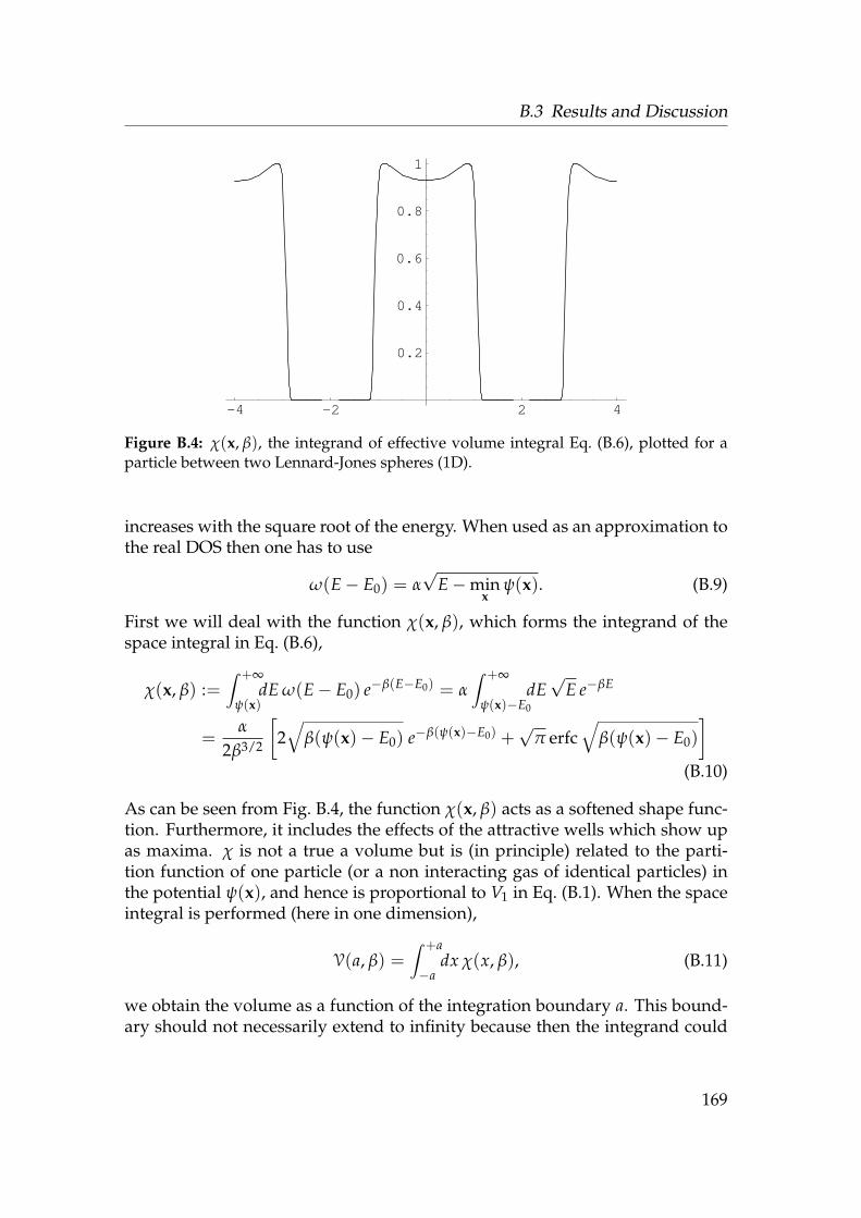
B.3 Results and Discussion
-4 -2 2 4
0.2
0.4
0.6
0.8
1
Figure B.4: χ(x, β), the integrand of effective volume integral Eq. (B.6), plotted for aparticle between two Lennard-Jones spheres (1D).
increases with the square root of the energy. When used as an approximation tothe real DOS then one has to use
ω(E− E0) = α√
E−minx
ψ(x). (B.9)
First we will deal with the function χ(x, β), which forms the integrand of thespace integral in Eq. (B.6),
χ(x, β) :=∫ +∞
ψ(x)dE ω(E− E0) e−β(E−E0) = α
∫ +∞
ψ(x)−E0
dE√
E e−βE
=α
2β3/2
[2√
β(ψ(x)− E0) e−β(ψ(x)−E0) +√
π erfc√
β(ψ(x)− E0)
](B.10)
As can be seen from Fig. B.4, the function χ(x, β) acts as a softened shape func-tion. Furthermore, it includes the effects of the attractive wells which show upas maxima. χ is not a true a volume but is (in principle) related to the parti-tion function of one particle (or a non interacting gas of identical particles) inthe potential ψ(x), and hence is proportional to V1 in Eq. (B.1). When the spaceintegral is performed (here in one dimension),
V(a, β) =∫ +a
−adx χ(x, β), (B.11)
we obtain the volume as a function of the integration boundary a. This bound-ary should not necessarily extend to infinity because then the integrand could
169
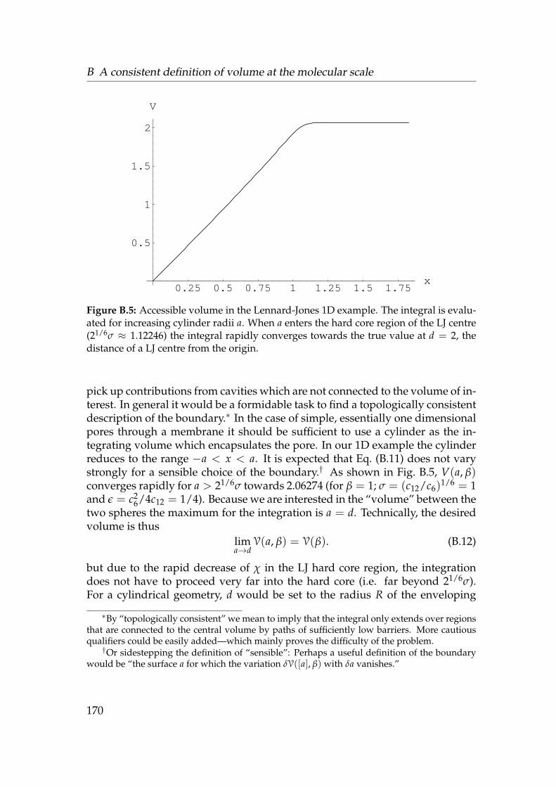
B A consistent definition of volume at the molecular scale
0.25 0.5 0.75 1 1.25 1.5 1.75x
0.5
1
1.5
2
V
Figure B.5: Accessible volume in the Lennard-Jones 1D example. The integral is evalu-ated for increasing cylinder radii a. When a enters the hard core region of the LJ centre(21/6σ ≈ 1.12246) the integral rapidly converges towards the true value at d = 2, thedistance of a LJ centre from the origin.
pick up contributions from cavities which are not connected to the volume of in-terest. In general it would be a formidable task to find a topologically consistentdescription of the boundary.∗ In the case of simple, essentially one dimensionalpores through a membrane it should be sufficient to use a cylinder as the in-tegrating volume which encapsulates the pore. In our 1D example the cylinderreduces to the range −a < x < a. It is expected that Eq. (B.11) does not varystrongly for a sensible choice of the boundary.† As shown in Fig. B.5, V(a, β)converges rapidly for a > 21/6σ towards 2.06274 (for β = 1; σ = (c12/c6)
1/6 = 1and ε = c2
6/4c12 = 1/4). Because we are interested in the “volume” between thetwo spheres the maximum for the integration is a = d. Technically, the desiredvolume is thus
lima→d
V(a, β) = V(β). (B.12)
but due to the rapid decrease of χ in the LJ hard core region, the integrationdoes not have to proceed very far into the hard core (i.e. far beyond 21/6σ).For a cylindrical geometry, d would be set to the radius R of the enveloping
∗By “topologically consistent” we mean to imply that the integral only extends over regionsthat are connected to the central volume by paths of sufficiently low barriers. More cautiousqualifiers could be easily added—which mainly proves the difficulty of the problem.†Or sidestepping the definition of “sensible”: Perhaps a useful definition of the boundary
would be “the surface a for which the variation δV([a], β) with δa vanishes.”
170

B.4 Conclusions
cylinder.
B.4 Conclusions
For simple systems the accessible volume can be calculated analytically but forcomplicated geometries and potentials this has to be carried out numerically. Atthis stage it is not clear if the effective volume differs significantly from conven-tional volume approximations. This method essentially calculates the partitionfunction for an ideal gas confined to the host system. From then on it would bestraightforward to derive other thermodynamic quantities as initial approxim-ations to the more complicated real fluid. The method would also have to beextended to calculate surface areas. Finally, electrostatic effects would have tobe considered. Clearly, the method presented here requires more work in orderto make it potentially useful. Its current marginal merit lies in demonstratingthe principle to define a volume based on statistical mechanics ideas.
171

B A consistent definition of volume at the molecular scale
172

C Analytical pore volume
The pore models used in Chapters 3 to 5 are geometrically simple objects soit should be possible to calculate their volume exactly, provided that they areassumed to be built from hard spheres with a defined radius. The “ruggedvolume” of the pore is understood as the space inside the cylinder which is notoccupied by a wall atom. Apart from re-entrant surfaces this is the solvent ex-cluded volume of the pore. A volume calculated in this way will be too largebecause it will also contain cusp regions that are not accessible to e.g. water mol-ecules, which have a finite diameter. More elaborate schemes to calculate thesolvent excluded surface (and thus the solvent excluded volume) take care ofthese re-entrant surfaces118,121 but the following calculations will neglect them.Incorporating re-entrant surfaces tends to smooth the surface so that it will moreresemble a smooth cylinder. Hence the shape of the pore is again approximately
(a) Solid rendering (b) Interfacial area
Figure C.1: Cylindrical pore intersecting a wall atom. (a) The pore volume can becalculated analytically as the volume of the enclosing cylinder minus the volume of theatomic sphere protruding into the cylinder. (b) The bounding surface of the intersectedsphere (coloured contour lines) is related to Viviani’s curve.316
173
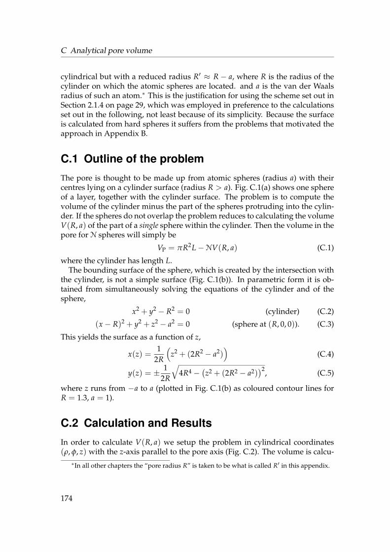
C Analytical pore volume
cylindrical but with a reduced radius R′ ≈ R− a, where R is the radius of thecylinder on which the atomic spheres are located. and a is the van der Waalsradius of such an atom.∗ This is the justification for using the scheme set out inSection 2.1.4 on page 29, which was employed in preference to the calculationsset out in the following, not least because of its simplicity. Because the surfaceis calculated from hard spheres it suffers from the problems that motivated theapproach in Appendix B.
C.1 Outline of the problem
The pore is thought to be made up from atomic spheres (radius a) with theircentres lying on a cylinder surface (radius R > a). Fig. C.1(a) shows one sphereof a layer, together with the cylinder surface. The problem is to compute thevolume of the cylinder minus the part of the spheres protruding into the cylin-der. If the spheres do not overlap the problem reduces to calculating the volumeV(R, a) of the part of a single sphere within the cylinder. Then the volume in thepore for N spheres will simply be
VP = πR2L−NV(R, a) (C.1)
where the cylinder has length L.The bounding surface of the sphere, which is created by the intersection with
the cylinder, is not a simple surface (Fig. C.1(b)). In parametric form it is ob-tained from simultaneously solving the equations of the cylinder and of thesphere,
x2 + y2 − R2 = 0 (cylinder) (C.2)
(x− R)2 + y2 + z2 − a2 = 0 (sphere at (R, 0, 0)). (C.3)
This yields the surface as a function of z,
x(z) =1
2R
(z2 + (2R2 − a2)
)(C.4)
y(z) = ± 12R
√4R4 −
(z2 + (2R2 − a2)
)2, (C.5)
where z runs from −a to a (plotted in Fig. C.1(b) as coloured contour lines forR = 1.3, a = 1).
C.2 Calculation and Results
In order to calculate V(R, a) we setup the problem in cylindrical coordinates(ρ, φ, z) with the z-axis parallel to the pore axis (Fig. C.2). The volume is calcu-∗In all other chapters the “pore radius R” is taken to be what is called R′ in this appendix.
174

C.2 Calculation and Results
ρa(φ) aR
φmax
(a) View perpendicular to pore z-axis
ρa(z) a(z)z R a
(b) View parallel to pore z-axis
Figure C.2: Geometry of an atomic sphere intersected by a cylindrical pore. The centresof the atomic spheres (one drawn as a circle) lie on the cylinder surface at radius R.The atomic hard sphere radius is a. In cylinder coordinates, the surface of a sphere isdescribed by the radial vector ρ(φ, z).
lated as the integral
V(R, a) =a∫−a
dz
φmax(z)∫−φmax(z)
dφ
R∫ρa(φ,z)
dρ ρ (C.6)
over the region bounded by the inner sphere surface ρa(φ, z) and the cylindersurface ρ = R. Elementary geometry yields
a(z) =√
a2 − z2 (C.7)
ρa(φ, z) = R
cos φ−
√(a(z)
R
)2
− sin2 φ
(C.8)
and for the maximum angle
φmax(z) = arcsina(z)
R. (C.9)
175
C Analytical pore volume
The evaluation of the Eq. (C.6) was performed in Mathematica317 by successiveintegration. The radial integral becomes (writing (a(z)/R)2 = sin2 φmax)
Iρ(φ, z) =R∫
ρa(φ,z)
dρ ρ
=R2
[1− cos 2φ− sin2 φmax(z) + 2 cos φ
√sin2 φmax(z)− sin2 φ
].
(C.10)
The angular integral (sweeping out the area at height z) is
Iφ(z) =
φmax(z)∫−φmax(z)
dφ Iρ(φ, z) = 2
φmax(z)∫0
dφ Iρ(φ, z)
= R2
[(arctan
(sin φ√
sin2 φmax(z)− sin2 φ
)sin2 φmax(z)
+ φ (1− sin2 φmax(z))
+
(√sin2 φmax(z)− sin2 φ−
√1− sin2 φ
)sin φ
)]φmax(z)
0
= R2(
φmax(z) + sin2 φmax(z)(π
2− φmax(z)
)− sin φmax(z)
√1− sin2 φmax(z)
).
(C.11)
When the substitutions
ξ :=Ra
and ζ :=za
(C.12)
sin φmax(z) =
√1− ζ2
ξ(C.13)
are made then Eq. (C.11) becomes
Iφ(z) =a2
2
(π(1− ζ2) + 2(ζ2 + ξ2 − 1) arccsc
(ξ√
1− ζ2
)
− 2√(1− ζ2)(ζ2 + ξ2 − 1)
). (C.14)
176

C.2 Calculation and Results
2 4 6 8 10Ra
0.44
0.45
0.46
0.47
0.48
0.49
3 V4 a3 Π
Figure C.3: Volume V(R, a) of a sphere of radius a protruding into a cylinder of radiusR, with the sphere centre lying on the cylinder surface. The volume of the part ofthe sphere inside the cylinder is shown for increasing cylinder radii. The volume ismeasured in the volume of the sphere 4
3 πa3; it only depends on the cylinder radius,measured in the sphere radius, R/a. For large cylinders it approaches the expectedresult of half the sphere volume.
Integrating yields the volume
V(R, a) =4πa3
3
× 16π
(3π +
√ξ2 − 1
[(10ξ2 − 11) E
(1
1− ξ2
)− (10ξ2 − 6)K
(1
1− ξ2
)])(C.15)
K and E are complete elliptic integrals of the first and second kind∗ and ξ =R/a [see (C.12)] is the cylinder radius, measured in units of the sphere radius.Eq. (C.15) is universal in that it only depends on the ratio R/a. As can be seen
∗Elliptic integrals:318 Complete elliptic integral of the first kind:
K(m) =∫ π/2
0
1√1−m sin2 θ
dθ, −∞ < m < 1.
177

C Analytical pore volume
from the graph of V(R, a) = V(R/a) in Fig. C.3, for large cylinder radii thecut-out volume approaches half the sphere radius because the cylinder surfaceincreasingly resembles a plane.∗ Unexpectedly, there is a minimum at aboutR/a ≈ 1.1. It is not relevant in our case, though, because R/a ≈ 1.1 describesa pore which has barely enough space to accommodate two non-intersectingwall atoms. The R/a ratios of the model pores range from 1.769 to 6.128 fora = 0.195 nm and 0.345 nm ≤ R ≤ 1.195 nm.†
C.3 Conclusions
The calculation shows that the exact volume of a cylinder with protruding, non-intersecting spheres can be easily calculated; for practical purposes this meansreading off a correction factor to the atomic sphere volume from Fig. C.3. Con-ceivably, a polynomial could be fitted to Eq. (C.15) to facilitate the volume cal-culation. In any case, the error made by approximating the protruding volumeof the atomic sphere as half the sphere volume is not greater than 10%. Also,inspection of 3D densities (the equivalent for the model pores to Fig. 6.10) in-dicated that water molecules trace out the solvent excluded MSMS surface,121
which incorporates re-entrant surfaces. The MSMS surface in turn is not veryrugged and thus well approximated by a cylinder. The MSMS/3D density sur-face and the calculations of this appendix justify the treatment of the modelpores as simple cylinders, which can be characterised by a single radius for thepurpose of volume calculations Section 2.1.4.
Complete elliptic integral of the second kind:
E(m) =∫ π/2
0
√1−m sin2 θ dθ, −∞ < m < 1.
∗For ξ → ∞ both E((1− ξ2)−1)) and K((1− ξ2)−1) become π2 ; the limit limξ→∞ V(ξ) =
23 πa3, however, is non-trivial as the approach of K and E towards π
2 differs.†Only in this chapter R denotes the radius of the cylinder surface. Previously R was the
effective radius of the van der Waals surface bounded pore, R − a, with 0.15 nm ≤ R − a ≤1.0 nm.
178

D Programs and scripts
This appendix describes some programs that were developed or modified in thecourse of this work. Where licensing permits, they are made available underthe GNU General Public License319 on the author’s website http://sbcb.bioch.ox.ac.uk/oliver/software/.
D.1 Simulation setup
D.1.1 pgeom
Usage
pgeom [OPTIONS] -R Router -P RP LP -M RM LM
Synopsis
pgeom calculates positions of pseudo-atoms in a model for a transmembranechannel and writes the structure to the file pore.pdb in PDB format, anda gromacs topology to pore.itp. The pore is constructed from concent-ric, stacked rings of spherical pseudo atoms. Typically, no bonds are gen-erated because the pore atoms are held at their equilibrium position by har-monic restraints (which are generated with the genpr program, which is part ofgromacs).
The user determines the dimensions of the mouth region and the constric-tion region. The pore profile is linearly interpolated between the radius of theconstriction RP and the radius of the mouth RM.
Options
-h show help-v be verbose (= -debuglevel 30)
-debug N set debuglevel (0. . . 100)-spec mspec atomic species for pore wall (see Tab. D.3)
-showspec show hard coded atomic species (see Tab. D.3)
-o pore.pdb pdb coordinate file
179

D Programs and scripts
-s pore.itp itp topology file
-R Router Outer radius of the model Router-P R L Pore region: inner radius R and length L-M RM LM Mouth region: largest inner radius RM and
length LM-b dmin dmax γmin γmax Option is repeatable. Form bonds with angle
γ when interatomic distance d satisfies dmin ≤d ≤ dmax (in A) and angle γmin ≤ γ ≤ γmax,0 ≤ γ ≤ 90
-c only write connectivity to output, no bondlength or kbond, kangle
-x neither connectivity nor bond length to output(isolated atoms)
-kB kbond force constant of bonds, in kJ ·mol−1 · nm−2
-kA kangle force constant of angles, in kJ ·mol−1 · rad−2
-cc center coordinates on cavitybox, not on unitcell
As an experimental feature, the pore volume can be calculated as described inAppendix B; the Lennard-Jones parameters are taken from the GROMACS forcefield. Setting any of the switches for profile calculation also enables the volumecalculations. All the following lengths are in nano metre (nm) not Angstrom.
-volume calculate pore volume-profile profile.dat calculate the profile R(z) in addition to the
volume and write to file-z1 z1 profile between z1 and z2-z2 z2
-Rmax Rmax integrate out to Rmax (also use for the totalvolume integration if -profile is set)
-npoints N number of points per dimension in the integrals-T T temperature in Kelvin [300]
-wca if set, only use the repulsive part of theLennard-Jones potential (split after Weeks,Chandler, and Andersen123)
-plot xfarbe output of the potential in z slices-nzplot Nslice number of plot slices for -plot
180
D.1 Simulation setup
mspec name symbol r/nm q/e
0 methane CH4 0.195 01 carbon C 0.140 +0.382 oxygen O 0.150 −0.38
Table D.3: Hard coded atomicspecies in pgeom.
Example
The hydrophobic pores of radius R, that were investigated in Chapter 3 weregenerated with the command line
pgeom -R 18 -P R 8 -M 10 8 -x -o pore.pdb -spore.itp
where Router = 1.8 nm (which is not functionally important because the porecomplex is embedded in a membrane mimetic slab), RM = 1.0 nm, LM = LP =0.8 nm (apart from the cases in Section 5.3.3 where LP was varied), and the poreradius R. Pores with hydrophilic pore walls were created by adding charges toselected atoms in the topology file pore.itp.
D.1.2 prepumbrella.pl
Usage
prepumbrella.pl [OPTIONS] --topology=topol.top--mdp=umbrella.mdp --index=refgroup.ndx--confstart=startingconfigs.dat --type="SPECIES"
Synopsis
Create run input files (tpr) for umbrella sampling runs, using gromacs (version3.2.1-LMB). Give the number of umbrella windows and either the length overwhich the windows are (equally) distributed or the minimum and maximumcoordinate. At the moment this only caters for 1D PMFs, e.g. just along z in apore or channel.
If only --length is given, the windows are created symmetrically to 0(which is then the centre of mass of the reference index group (type ‘com’ or‘com t0’ in the ppa)). If --min and --max or --length and either one of--min or --max are given, the window centres are offset accordingly (still relat-ive to the reference group’s centre of mass). The window width ∆z is calculatedas length L = max z−min z divided by the number of windows N, ∆z = L/N.
Unless overridden from the commandline, the force constant is chosen so thatan ion in window i can freely diffuse into an adjacent window i + 1 or i− 1. The
181

D Programs and scripts
energetic barrier to this diffusion is given by --barrier (and is the energy ofthe umbrella potential at zi +
32 ∆z, i.e. the centre of the neighbouring window).
Set the temperature to the one set for the simulations.This script requires all the files needed to run grompp so that it can create the
tpr files for all the windows and a special list of starting configurations, cus-tomarily named conf.dat. It creates a ppa file using a hard coded template.The grompp mdp file should have the proper run length (e.g. 1 ns) and typicallyneither trr nor xtc output are required.
Implicit assumptions
• Currently we assume that the direction of the sampled coordinate is(0, 0, 1), i.e. the z-axis.
• the configuration list contains absolut positions
• the center of mass (com) must be supplied in the configuration list
• max, min, and length are relative to the com of the ref group
Options
Defaults in brackets, for most options abbreviations can also be used.
--help this help--help-targets list of known target systems (for
--targetsystem)--help-config format of the starting configuration file (for
--confstart); see below--version version number of prepumbrella.pl (quote when
submitting a bug report)--verbose chatty output
--debug=INTEGER set debug level (> 9 switches off error checks, >11 grompp is not run at all, only commandlineshown)
Input files (all must exist):
--topology=FILE gromacs topology [topol.top]--mdp=FILE grompp input with run parameters
[grompp.mdp]--index=FILE index file containing the reference group
[pull.ndx]
182

D.1 Simulation setup
--confstart=FILE list that describes available starting conforma-tions (see below for format) [conf.dat]
--np=INTEGER number of processors to write tpr files for [1]
Output:
--Project=DIRECTORY place all window directories under DIRECTORY[.]
--prefix=STRING output tprs are named STRINGn.nnnn.tpr(where n.nnnn is the centre of the umbrella win-dow in nm) if the standard --format string isused []
--format=PRINTFSTRING pattern to create output filenames. May containone ‘%s’ (for prefix) and one ‘%f’ for the um-brella centre (see printf(3)) [%s%+.4f]
--qsuball=FILE script that contains qsub commands to submitall windows through a queuing system
--targetsystem=SYSTEM create run script(s) for the given target systems;can be given repeatedly to produce more thanone type of runscript. Use --help-targetsfor a list of valid SYSTEMs and the values thatthey define (with --verbose) [local]
Umbrella windows:
--type=STRING name of the particle, eg Na, Cl, NA, . . . (as usedin the input files)
--nwindows=INTEGER number of umbrella windows [20]--length=FLOAT length to cover with windows, symmetrically to
the reference group’s centre of mass. Alternat-ively, set --min and --max.
--min=FLOAT relative to reference group centre of mass, in nm--max=FLOAT relative to reference group centre of mass, in nm
--kUmbrella=FLOAT force constant of the harmonic umbrella poten-tial in kJ · mol−1 · nm−2; overrides programchoice
--Temperature=FLOAT temperature of the simulation in Kelvin[298.0]
--barrier=FLOAT barrier to move to the centre of an adjacent win-dow in kT [1.5]
183

D Programs and scripts
Format of the starting configuration file
The configuration file conf.dat contains a header section where parametersare set, and a list of possible starting configurations. prepumbrella.pl uses thelist of starting configurations to find those which have a particle of interest closeto the centre of an umbrella window. It then looks up the corresponding startingstructure file (in gro format) from the list and uses it to create binary run inputfile (tpr) by running grompp.
; comment (same as in Gromacs mdp files); all entries must be on one line; ’@’ lines set variables@ var = valuefilename particle_type atom_nr pos_x pos_y pos_zfilename particle_type atom_nr pos_x pos_y pos_z...
filename full path to the gro or pdb fileparticle type name used in gromacs, eg Na, Cl, SOLatom nr atom id, number in gro or index filepos x|y|z coordinates of the particle in nm
Required variables Variable assignments are introduced by an @-sign at thebeginning of the line; spaces around ‘=’ are mandatory. Required variablesmust be given in the configuration file.
center of mass = x y z center of mass of the reference group
Optional variables If no values are given the program defaults are chosen(given in brackets) and the program issues a warning. A cylindrical confine-ment potential is only activated if both RConfine and KConfine are non-zero.
reference group = group reference group from index file [protein]reftype = com t0|com center of mass from initial frame or always
from the current frame [com t0]RConfine = R use a confinement potential outside a radius R
nm [0.0]KConfine = k and a harmonic force constant k kJ ·mol−1 ·
nm−2 [4500.0]
184

D.1 Simulation setup
prepconflist.pl (Appendix D.1.3) can be used for setting up the configuration listfrom trr frames.
Bugs and Limitations
• Runscripts are generated for different target system environments andthe specifics are hard coded in the script itself. See the source itself and--help-targets --verbose. The target system complex should be-come configurable through an external XML file.
• Only single ions as pulled groups are tested.
• conf.dat should be XML.
• The umbrella ppa file should be a template and not hard coded.
• Dirty hack: if there is an index file named exactly ‘index.ndx’ in thecurrent directory then it is automatically picked up at the grompp stage;this allows for using non-standard groups in the mdp file.
Example
conf.dat contains all required variables and a list of starting configura-tions, with the starting configurations themselves accessible. The index filerefgroup.ndx contains the index group protein, relative to whose centreof mass the umbrella windows are placed. The topology and related files arefound two directories above the current one, with the main topology beingchl.top. The molecular dynamics run input file umbrella.mdp is similar toone used for equilibrium simulations with the exception of a shorter run length(typically about 1 ns, no trajectory output, and when starting from structurefiles with velocities, gen vel = no and unconstrained-start = yes). Inthe example, a Na+ ion (with the general name Na) is to be umbrella sampled.The command line
source /opt/gromacs/3.2.1-LMB/i686-pc-linux-gnu/bin/GMXRCprepumbrella.pl --topology=../../chl.top--mdp=umbrella.mdp --index=refgroup.ndx--confstart=conf.dat --Project=0R55/Na--prefix=Na0R55z --type=Na --nwindows=101--min=-0.9 --max=0.9 --Temperature=300--targetsystem=workstations --qsuball=submitall.sh
will have prepumbrella.pl construct 101 separate input files for mdrun; eachof these windows can be run independently from the others thus allowing
185

D Programs and scripts
massively parallel execution on clusters or compute farms. Depending on thetarget system, run input files for a queuing system are also created, which allowsubmission of all 101 jobs through execution of a single script, submitall.sh.Note that the script requires a working gromacs environment to create the runinput files.
After these jobs have finished, g wham is run on all result files *.pdo.gz asdescribed in Appendix D.2.5.
D.1.3 prepconflist.pl
Usage
prepconflist.pl [OPTIONS] file1.gro [file2.gro...]
Synopsis
prepconflist.pl creates the file list which forms the major content of the input file(conf.dat) to prepumbrella.pl. It reads all files given on the command line andwrites matches to the output file (with --append it appends to the output file).
Options
The options can be abbreviated; defaults are given in [].
--help help--verbose (alias for DEBUGLEVEL= 3)--version print version id
--debug=DEBUGLEVEL 0 (almost) quiet, < 0 silent, 1 . . . 3 verbose, > 5really debugging stuff (20 max) [1]
--output=FILE output gro file [conf.list]--append append to output file (do not overwrite)
--atomname=STRING name of the pulled atom in the gro file [NA]--z1=FLOAT only list starting positions with z coordinate--z2=FLOAT between z1 and z2 (box coordinates in nm).
--radius=FLOAT Also, only list them when they are within a cyl-inder of radius R which is centered on the cen-ter of mass.
--xcom=FLOAT ref. group centre of mass x-coordinate (nm)--ycom=FLOAT ref. group centre of mass y-coordinate (nm)
186

D.1 Simulation setup
--zcom=FLOAT ref. group centre of mass z-coordinate (nm), butthis is not used at the moment as the cylinder isalways taken to be parallel to the z-axis
Example
First we generate a selection of equilibrium configurations of the whole sys-tem by dumping snapshots from an equilibrium trajectory of the system.
mkdir startecho -e ’0\n’| trjconv -tu ns -b 2 -sep -s ../../chl md.tpr-f ../../chl lay water md.trr -o start/na.gro
Here a trr file is used, which allows to start with velocities. About 300 framesare typically required. The whole system is required (which is selected bychoosing ‘0’). The index for the reference group is created through
make ndx -f ../../chl md.tpr -o refgroup.ndx
Typically, the whole protein is chosen. The centre of mass of the reference groupcan be calculated with
g traj -com -f start/na 1.gro -s ../../chl md.tpr-n refgroup.ndx -ox com.xvg
and is found as the single entry in com.xvg.Then prepconflist.pl goes through the configurations and generates a list re-
lating the position of a particle type of interest (e.g. ion or water oxygen) to thefile where it was found.
prepconflist.pl --xcom=2.2 --ycom=2.3--radius=0.8 --z1=1.7 --z2=6.4 --atomname=Na--output=conf.list --verbose start/*.gro
To reduce the number of entries one can restrict the volume in which particlesare searched for. The volume is a cylinder centered on the centre of mass ofthe reference group, extending from z1 = 1.7 nm to z2 = 6.4 nm with a radiusR = 0.8 nm. The resulting conf.list can be appended to the header sectionof a conf.dat file (see Appendix D.1.2).
187
D Programs and scripts
D.2 Analysis
D.2.1 g count
Usage
g count -f trajectory.xtc -s topol.tpr [OPTIONS]
Synopsis
g count counts the numbers of molecules within a cylindrical region as a func-tion of time. It takes an index file with atomnumbers and chooses the moleculesthat these atoms belong to (or optionally (with option -nom) it simply takesall atoms in the index) and generates an output file with the number of mole-cules/atoms which are present in the cavity a each time frame.
The output data file (option -dat) contains for each time step t the numberof particles in the cavity (the pore occupancy N(t)), the concentration c(t), andthe mass density ρ(t).
column: 1 2 3 4quantity: t N(t) c(t) ρ(t)units: ps mol · l−1 g·cm−3
Density and concentration are calculated from the volume of the cavity,
V = R2effπ(z2 − z1) (D.1)
where Reff is the apparent accessible radius (corrected with wall atom radiusrA = σAA/2 (approximately the van der Waals radius), water radius rwater ≈0.14 nm, and the distance between the centre of a wall atom A (typically, aunited atom methane CH4) and the water oxygen (OW), dwall-water = σAOW . σcome from the Lennard-Jones potential of the wall atom and the water oxygen.
Reff = R− dwall-water + rwater; (D.2)
R is the radius of the pore, measured from the atomic center of a wall atom tothe pore axis. The pore radius R (which is quoted throughout this work) is
R = R− rA, (D.3)
and it is the radius of the cylinder formed by the solvent accessible van derWaals surface.∗ Thus, the radius correction could be calculated from the force∗Because of the atomic roughness of the pore wall it is not strictly correct to speak of a single
pore radius—depending on the angle the distance from the pore axis to the surface varies. R isthe shortest radial distance in the pore and hence represents a lower bound on the true averagepore radius.. See also the discussion in Appendix C.3.
188

D.2 Analysis
field (i.e. σ) as
δR =12
σAA − σAOW + rwater (D.4)
This approach turns out to be somewhat imprecise and δR was then consideredas an adjustable parameter which was determined as described in Section 2.1.4on page 29 by considering a large pore and matching the volume resultingfrom the above calculation and an integration of the local density (producedby g ri3Dc, described in Appendix D.2.3).
The -track index file contains the atom ids of all atoms that were at leastfor -tau τ ps in the cavity (entry [ * tracked ]). The entry [ * cavity ]contains all atoms that were for at least one time frame in the cavity. Entriescontaining molecule numbers are titled [ * molecules ].-tdat writes a data file containing all atoms or molecules in the cavity and
their total residency time. Format:
column: 1 2 3 4 5quantity: atom nr molecule nr name total residency time Tres Tres/Tunits: ps
Defaults If no values are given for the point on the axis (option -cpoint)then the center of the initial box is taken. If no radius -R R is given, the max-imum radius fitting in the box is chosen. z1 and z2 default to the full box lengthin z-direction.
Files-f traj.xtc Input Generic trajectory: xtc trr trj gro g96 pdb-s topol.tpr Input Structure+mass(db): tpr tpb tpa gro g96
pdb xml-o c numbers.xvg Output xvgr/xmgr file
-dens c density.xvg Output, Opt.xvgr/xmgr file-conc c conc.xvg Output, Opt.xvgr/xmgr file-dat cavity.dat Output Generic data file
-tdat c track.dat Output Generic data file-n index.ndx Input, Opt. Index file
-track c track.ndx Output, Opt.Index file
Other options-h bool no Print help info and quit
-nice int 0 Set the nicelevel
189

D Programs and scripts
-b time -1 First frame (ps) to read from trajectory-e time -1 Last frame (ps) to read from trajectory-dt time -1 Only use frame when t MOD dt = first time (ps)-w bool no View output xvg, xpm, eps and pdb files-m bool yes index contains atoms, but g count counts the mole-
cules-axis vector 0 0 1 Vector pointing parallel to the pore axis
-cpoint vector 0 0 0 Point on the pore axis-R real -1 Radius of the cylindrical pore cavity-z1 real -1 Confine waters to have a z coordinate larger than z1,
and-z2 real -1 smaller than z2-tau real 10 Total time (ps) that a particle has to be in the cavity at
least so that it is tracked-dR real 0.03 Correct water-accessible cavity volume
Known problems and caveats
• -m behaves differently from the standard usage within the g * programs—it figures out for itself what the molecules are and does not need moleculenumbers but atom ids.
• -m is the default behaviour!
• When counting ions you must use -nom !
• The density is calculated as 〈M〉 /[R2effπ(z2 − z1)] where 〈M〉 is the aver-
age mass in the pore cavity—so it makes only sense if this approximatesthe true cavity volume.
• The default volume/radius correction is specific for methane pseudoatoms (ffgmx, ffG43a1) and SPC water.
• The program is only tested with pore axis parallel to z-axis (0,0,1).
Example
Suggested use for water. Create an index file for the water molecules:
echo -e "keep 0\ndel 0\nr SOL\nq\n"| make ndx -f in.pdb -o sol.ndx
Then analyse the water molecules in a trajectory traj.xtc with
g count -m -f traj.xtc -s topol.tpr -n sol.ndx
190

D.2 Analysis
D.2.2 g flux
Usage
g flux -f trajectory.xtc -s topol.tpr [OPTIONS]
Synopsis
g flux calculates the flux of molecules (or atoms) through a cylindrical regionas a function of time. It takes an index file with atomnumbers and choosesthe molecules that these atoms belong to (or optionally (with -nom ) it simplytakes all atoms in the index) and generates an output file with the number ofmolecules/atoms at each time frame.
Definition of observables
Flux The flux Φ is the number of particles permeating the pore per unit time.It is calculated from the total number of permeating particles M during a simu-lation of length T as
Φ =MT
. (D.5)
M counts particles in both directions (“up” or “+” and “down” or “−”), i.e.M = M+ −M− where M+ ≥ 0 and M− ≤ 0. The fluxes are
Φ+ =M+
T≥ 0 (D.6)
Φ− =M−
T≤ 0 (D.7)
Φ =|Φ+|+ |Φ−|. (D.8)
In equilibrium, the net flux Φ+ + Φ− is zero because on average there is no netforce favouring either direction. In practice, there tends to be a very small bias(of the order of 0.1% of Φ) towards negative fluxes which might be related to therescaling of the particle positions due to the constant-pressure weak-couplingscheme.
The cumulative flux
F(t) :=∫ t
0dt′Φ(t′) =
t
∑t′=0
M(t′)
is calculated from the instantaneous flux Φ(t) = M(t)/∆t over one time step ∆tand counts the number of permeation events up to time t.
191

D Programs and scripts
Permeation time The residency time τp,i(t) for a pore-permeating particle ithat entered the pore time at t′i and exited at t is
τp,i(t) = t− t′i. (D.9)
The average permeation time τp(t) for all M(t) particles that permeated thepore between t′i and t > t′i is calculated as
τp(t) =1
M(t)
M(t)
∑i=1
(t− t′i),
i.e. at each time the length of the permeation events that completed at this stepare averaged. The cumulative average permeation time is
⟨τp(t)
⟩=
∑tt′=0 M(t′)τp(t′)
∑tt′=0 M(t′)
and can be used to assess the convergence of the mean permeation time
〈τp〉 ≡⟨τp(T)
⟩. (D.10)
Algorithm
The algorithm to detect the permeating particles can be described as “checkon exit.” If ‘O’ denotes the space outside of the pore and ‘I’ the inside, thenonly trajectories O→I→O are counted as complete transitions through the pore;I→O→I are periodic boundary trajectories. Any enter event for a particle isrecorded; on a later exit it is determined if it left the pore volume on the sideopposite to the influx event (a permeation event) or on the same side (not asuccessful permeation).
In the following, the pore is assumed to be oriented parallel to the z-axis. Thefaces of the cylindrical pore are at z1 < z2.∗ For any given molecule i at positionx = (x, y, z) compare the position at time step t and at the previous step t− 1.
1. A molecule crosses a boundary at zm (m = 1, 2) if
min(z(t− 1), z(t)
)< zm < max
(z(t− 1), z(t)
)is true.
∗A generalisation to pore axes pointing along other vectors than (0, 0, 1) is straightforwardbut was not necessary in the cases discussed here.
192

D.2 Analysis
2. Given a boundary crossing at step t, determine the type of the crossing(enter or exit event). The type is recorded as the “divergence” D
D =
+1 if z1 < z(t) < z2 (O→I, entering)−1 if z(t) < z1 ∨ z(t) > z2 (I→O, exiting)
3. Determine the direction u of the crossing, relative to the pore axis p
u = sgn([x(t)− x(t− 1)] · p
),
where u = +1 signifies a flow “up” and u = −1 a flow “down.”
4. Characterise the crossing event, and determine permeation events:
Influx event D = +1 Only trajectories O→I→O can represent per-meation events, i.e. they always start with an influx event, so for theparticle i that crossed a boundary at t store the influx event (i, t, u(t)).
Efflux event D = −1 An efflux event signals a permeation event if theparticle exits through the face opposite to the one it entered a previ-ous time t′. Compare the direction of the efflux u(t) with the one ofthe influx u(t′), which was stored as the influx event (i, t′, u(t′)).
u(t) = u(t′)⇒ permeation event.
Then the recorded event (i, t′, u(t′)) is erased.
Output
The -dat file contains instantaneous values at each time step t whereas the-cdat data file records the corresponding cumulative values up to t,
column: 1 2 3 4 5 6-dat: t Φ+(t) + Φ−(t) Φ+(t) Φ−(t) Φ(t) τp(t)-cdat: t F+(t) + F−(t) F+(t) F−(t) F(t)
⟨τp(t)
⟩units: ps ps−1 ps−1 ps−1 ps−1 ps
The index file -ncr lists the indices of all molecules that permeated the poresuccessfully. The data file -res contains a histogram of permeation times τp.
Options
Files-f traj.xtc Input Generic trajectory: xtc trr trj gro g96 pdb
193
D Programs and scripts
-s topol.tpr Input Structure+mass(db): tpr tpb tpa gro g96pdb xml
-n index.ndx Input, Opt. Index file-o flux.xvg Output xvgr/xmgr file
-dat flux.dat Output Generic data file-cdat cflux.dat Output Generic data file-ncr crossed.ndx Output Index file-res residency.dat Output Generic data file
Other options-h bool no Print help info and quit
-nice int 0 Set the nicelevel-b time -1 First frame (ps) to read from trajectory-e time -1 Last frame (ps) to read from trajectory-dt time -1 Only use frame when t MOD dt = first time (ps)-w bool no View output xvg, xpm, eps and pdb files-m bool yes index contains atoms, but g flux counts the molecules
-axis vector 0 0 1 Vector pointing parallel to the pore axis-cpoint vector 0 0 0 [hidden] Point on the pore axis
-z1 real -1 Confine waters to have a z coordinate larger than z1,and
-z2 real -1 smaller than z2
Known problems and limitations
• -m behaves different from the standard usage within the g * programs—itfigures out for itself what the molecules are and does not need moleculenumbers but atom ids.
• -m is the default behaviour!
• Despite appearance it only makes sense to specify a pore axis approxim-ately parallel to the z-axis because we only really base the definition of theboundaries on z coordinates.
Example
Suggested use for water: Create an index file for the water molecules:
echo -e "keep 0\ndel 0\nr SOL\nq\n"| make ndx -f in.pdb -o sol.ndx
194
D.2 Analysis
Then run
g flux -m -f traj.xtc -s topol.tpr -n sol.ndx-cpoint 2.3. 2.3 2 -z1 1.9 -z2 2.7
and analyse the output in flux.dat, cflux.dat, and residency.dat.
D.2.3 g ri3Dc
Usage
g ri3Dc -f trajectory.xtc -s topol.tpr [OPTIONS]
Synopsis
g ri3Dc places a 3D grid into a simulation box and counts the number of mole-cules (typically water) in each cell over a trajectory. The rectangular grid is largeenough to encompass a cylinder of given radius and height (specify radius R,lower and upper z, and a point on the pore axis (which is always parallel to thez-axis). If no parameters are given for the cylinder, a cylinder is fit into the sim-ulation box. The cylinder (and thus the grid) is fixed. The spatial resolution canbe given either as one number for all three dimensions (cartesian coordinates;unit is nm) or separately as three (Note: (1) It is recommended to use at least thesame grid spacing in x and y (which is compatible with a cylindrical symmetryalong z)). (2) The exact dimensions of the grid (radius etc) are re-adjusted tointegral numbers of the grid spacing.) At the end, a density map (occupancytime over total simulation time Tcell/T) is written to the grid file.
The output is the number density, averaged over the trajectory. Read this fileinto a ri3Dc, the grid analysis program, and produce radial distribution func-tions, density plots, pore profiles etc. The grid data is written as a binary file (inthe machine independent xdr format). a ri3Dc has an option to write it out asascii text.
Options
Files-f traj.xtc Input Generic trajectory: xtc trr trj gro g96 pdb-s topol.tpr Input Structure+mass(db): tpr tpb tpa gro g96
pdb xml-n index.ndx Input, Opt. Index file
-grid gridxdr.dat Output Generic data file
195
D Programs and scripts
Other options-h bool no Print help info and quit
-nice int 0 Set the nicelevel-b time -1 First frame (ps) to read from trajectory-e time -1 Last frame (ps) to read from trajectory-dt time -1 Only use frame when t MOD dt = first time (ps)-w bool no View output xvg, xpm, eps and pdb files-m bool yes index contains atoms, but g ri3Dc counts the mole-
cules-cpoint vector 0 0 0 Point on the central symmetry axis of the grid
-R real 0 Maximum radius that should be contained in the grid-z1 real 0 Center grid between z1, and ...-z2 real 0 z2 (these boundaries are kept fixed!)
-delta vector0.02 0.02 0.02 Spatial resolution in X, Y, and Z (in nm)
-dtweight bool yes [hidden] Weigh counts with the time step (yes) orcount all equally (no)
-subtitle string Some text to add to the output graphs
Caveats and known limitations
• The program guarantees to use the user supplied grid spacing. If the otherdimensions are incommensurable with Delta they are changed to comply.
• If you want radial distribution functions (yes, you do!) always useDelta[XX] == Delta[YY] to keep the cylindrical symmetry
• z-axis is the only allowed axis (and this will probably not change in thefuture)
• -m behaves different from the standard usage within the g * programs –it figures out for itself what the molecules are and does not need moleculenumbers but atom ids.
• -m is the default behaviour. It works nicely with a SOL index file but morecomplicated solvents are untested.
• For ions you haved to use the -nom option!
• The XDR file is not compressed.
• Even the developer mistypes the name frequently
196

D.2 Analysis
Example
Suggested use for water. Create an index file for the water molecules with
echo -e "keep 0\ndel 0\nr SOL\nq\n" \| make ndx -f in.pdb -o sol.ndx
Then run
g ri3Dc -m -f traj.xtc -s topol.tpr -n sol.ndx-delta 0.05 -grid grid.dat
(-m is the default but is shown here because the usage is different from thestandard gromacs analysis programs). The 3D density is in file grid.dat andcan be analysed with a ri3Dc (see Appendix D.2.4).
D.2.4 a ri3Dc
Usage
a ri3Dc -grid gridxdr.dat [OPTIONS]
Synopsis
a ri3Dc analyses a 3D grid produced by g ri3Dc. The 2D projections are writtenin a format suitable for the fast 2D density plotter xfarbe.223 It also writes a para-meter file ‘XFarbe’ which can be used automatically by setting the environmentvariable ‘XAPPLRESDIR=.’, and then running xfarbe, e.g. ‘xfarbe rzp.dat’ All geometry options (radius, z1, z2) that are not set and appear as ’0’ are setfrom the grid dimensions once it is read in. The -dump option converts a bin-ary grid file into ascii txt. The -plt option produces a binary density file forgOpenMol, which you might have to rename to xxx.plt. vmd since version1.8.2 can also read plt files and render them. The average density in the testcylinder is printed on std out, using the set units.
197
D Programs and scripts
Output
density z-averaged n(x, y) = Lz−1 ∫ dz n(x, y, z)
density y-averaged n(x, z) = Ly−1 ∫ dy n(x, y, z)
density x-averaged n(y, z) = Lx−1 ∫ dx n(x, y, z)
density radially averaged n(r, z) = (2π)−1∫
dφ n(r, φ, z)pore profile (z, RG(z), RG(z)/R)radial distribution function(rdf)
n(r) = (2π Lz)−1∫
dφ dz n(r, φ, z)
axial distribution function (zdf) n(z) = (LxLy)−1∫
dx dy n(x, y, z)n(r) and n(z) are averaged densities (normalisation is straightforward in orderto turn them into ‘real’ probability distributions). The local density axial dis-tribution function -lzdf averages over all occupied grid cells per z-slice anddivides by an effective area which is determined from the ‘radius of gyration’of the density
R2G(z) :=
2∫ 2π
0 dφ∫ R′
0 dr r3 n(r, φ, z)∫ 2π0 dφ
∫ R′0 dr r n(r, φ, z)
(2.48)
as explained in Section 2.1.4. This radius is a good approximation to the poreprofile. The density itself is in the lzdf.xvg file.
For diagnostic purposes one can also plot the radial distributions of the un-occupied cells (holes in the grid) in order to find suitable grid spacings.
Options
Files-grid gridxdr.dat Input Generic data file
-profile profile.xvg Output xvgr/xmgr file-xyp xyp.dat Output Generic data file-xzp xzp.dat Output, Opt.Generic data file-yzp yzp.dat Output, Opt.Generic data file-rzp rzp.dat Output Generic data file-rdf rdf.xvg Output xvgr/xmgr file-zdf zdf.xvg Output xvgr/xmgr file-lzdf lzdf.xvg Output xvgr/xmgr file-hxyp hxyp.dat Output, Opt.Generic data file-hrzp hrzp.dat Output, Opt.Generic data file-hrdf hrdf.xvg Output, Opt.xvgr/xmgr file-dump gridasc.dat Output, Opt.Generic data file-plt plt.dat Output, Opt.Generic data file
198

D.2 Analysis
Other options-h bool no Print help info and quit
-nice int 0 Set the nicelevel-R real 0 Maximum radius that should be contained in the grid-z1 real 0 Center grid between z1, and ...-z2 real 0 z2 (these boundaries are kept fixed!)
-delta vector0.02 0.02 0.02 [hidden] Spatial resolution in X, Y, and Z for resampling
(in nm)-minocc real 0 [hidden] The occupancy of a cell must be larger than
this number so that it is counted as occupied when cal-culating the volume, effective radius and local dens-ity axial distribution -lzdf. This is given in the chosenunits (see -unit).
-subtitle string Some text to add to the output graphs-mirror bool yes mirror the radial projection P(r,z) to create the impres-
sion of a full view of the pore-unit enum unity divide number density (in nm-3) by 1, the density of
SPC water at 300K and 1 bar, in mol/l or in Ang-strom-3. Allowed values: unity, SPC, molar orAngstrom
-xfarbe-maxlevel real 48.4841 xfarbe will plot 15 equally space level up to this dens-ity (the unit must be the same as for the -unit option!)Default is 1.5 SPC bulk.
-holes bool no [hidden] calculate all hole distribution functions, us-ing default filenames
-radnr int 0 [hidden] block-average the first rad ba nr radialbins...
-radstep int 1 [hidden] ...in blocks of rad ba step
Known limitations
• The radial bin width DeltaR is fixed to (Delta[XX]+Delta[YY])/2). In anycase one should never have different bin widths in X and Y.
• There are still a few hidden options of questionable usefulness. Res-ampling (=changing Delta) is not implemented yet.
• gOpenMol plt binary file comes out with wrong suffix
• note: -minocc also influences -lzdf
199

D Programs and scripts
D.2.5 g wham
Usage
g wham [OPTIONS] file1.pdo.gz file2.pdo ...
Synopsis
g wham is an analysis program that implements the Weighted Histogram Ana-lysis Method (WHAM).174,175 It is intended to analyze .pdo files generated bymdrun with umbrella sampling to create a potential of mean force (PMF).
Data files (pdo) may be gzipped and are simply listed on the command-line. Only frames between the begin time -b and the end time -e are in-cluded, giving the opportunity to discard an initial equilibration phase (-1means ‘no limit’). The program will discard any data that is outside of theinterval [min z; max z]. The program will output the true lowest and highestcoordinate values after completion, so these values can be used the next time oralternatively with -noprof only min and max are calculated in a first pass.Output:The first column in both data files is the position z along the sampled coordinatein nm. The histogram contains the data for each individual window. The profile-o contains the unbiased distribution Z(z) and the PMF G(z)/kT = − ln Z(z):
column: 1 2 3quantity: z Z(z) G(z)units: nm kT
Files-o profile.xvg Output xvgr/xmgr file
-hist histo.xvg Output xvgr/xmgr file
Other options-h bool yes Print help info and quit
-nice int 19 Set the nicelevel-b time -1 First frame (ps) to read from trajectory-e time -1 Last frame (ps) to read from trajectory-tu enum ps Time unit: ps, fs, ns, us, ms, s, m or h-min real 0 Minimum coordinate in profile-max real 0 Maximum coordinate in profile-bins int 100 Number of bins in profile-prof bool yes Calculate profile, when ’no’ only calculate min and
max
200

D.2 Analysis
-temp real 298 Temperature-flip bool no Combine halves of profile-tol real 1e-05 Tolerance
History
g wham is part of the gromacs package. It was broken in version 3.2.1. Itwas modified to allow processing of output from umbrella sampling data frommdrun and the format version was incremented to 3.2, breaking any back-ward compatibility. The new version can read data files in uncompressed andGNUzipped format. It allows sub-selections of the data through the -b and -eflags. The code has been cleaned up and modularised, making future enhance-ments for higher dimensional WHAM easier.
Bugs and Limitations
• This version of g wham reads pdo files with version number 3.2. It will notread version 3.0 (produced by the mdrun binary from the official gromacs3.2.1 distribution).
• Only 1D PMF along a box axis implemented.
• Symmetric profiles (-flip) do not work.
Example
The first 100 ps of data are discarded as equilibration (this is necessary but oneshould check for each system by calculating PMFs for different time windows,using the -b and -e options; the equilibration phase can be significantly longerthan the data collection, e.g. 2.5 ns equilibration and 0.5 ns data). First theminimum and the maximum z values need to be found because they are needfor setting up the histogram. The -noprof option reads in all data and printsthe limits on standard output:
find . -name ’*.pdo*’| xargs g wham -noprof -temp 300 -b 100
With these limits (in this example, −0.9 nm ≤ z ≤ 0.9 nm) the WHAM proced-ure is carried out with
find . -name ’*.pdo*’| xargs g wham -temp 300 -b 100 -min -0.9-max 0.9 -tol 1e-5 -bins 500 -o pmf.xvg -histhistogram.xvg
201

D Programs and scripts
The tolerance for the self-consistent solution of the WHAM equations is import-ant. 10−3 kT is not enough. 10−5 kT is the minimum that resolves a test-inputstep function (generated with fakepmf, see Appendix D.3.2). It is recommenedto plot the PMF for different values of the tolerance and check its convergence.The PMF is found in the output file pmf.xvg, and the histograms from all inputfiles are found in histogram.xvg. They can be displayed with xmgrace,
xmgrace -block pmf.xvg -bxy 1:3xmgrace -nxy histogram.xvg
D.3 Trajectory generation
D.3.1 Confinement in mdrun
Synopsis
mdrun from version 3.2.1 of gromacs was modified in the parts concerned withumbrella sampling in order to make it work together with the WHAM analysisprogram g wham and to add an experimental cylindrical confinement potential.The output format was changed (current version of the format is now 3.2 whichis incompatible with the previous version 3.0 but can be read by the modifiedversion of g wham). mdrun and g wham are now versioned 3.2.1-LMB.
Umbrella sampling is activated with the -pi option. An input file pull.ppamust be provided, which controls all aspects of umbrella sampling, an indexfile which defines the group that is sampled, and a standard run input tpr file.Umbrella sampling can be performed in parallel.
Confinement potential
A cylindrical confinement potential was added. Outside the pore region asampled particle is not bounded in the plane perpendicular to the umbrella po-tential. Thus the 1D PMF is not well defined and any results from WHAM aremeaningless.169,170 With a confinement potential, starting from outside a con-finement radius RC in addition to the umbrella potential, it should be possibleto obtain a defined PMF. The flat-bottomed confinement potential has the form
UC(x) = 12 kC Θ[ρ(x)− RC] (ρ(x)− RC)
2, (D.11)
where ρ(x) denotes the distance from the line along which the umbrella win-dows are distributed (typically, just the z-axis), and kC is the harmonic forceconstant.
202

D.3 Trajectory generation
Input file format
The input ppa file for umbrella sampling needs to comply to the followingexample format (lines starting with ‘;’ are comments and are ignored by theparser).
; Input for umbrella sampling; version: Gromacs 3.2.1-LMB
verbose = yesruntype = umbrella ; umbrella samplingpulldim = N N Y ; restrict in Z dimensionreftype = com_t0 ; compute center of umbrella potential
; relative to initial COM ofreference_group = Protein ; the reference group
; Umbrella sampling; group which is subjected to the umbrella potential; (see the index file):group_1 = NA_-0.337K1 = 3909.50; ; kJ / (mol nmˆ2)Pos1 = 0.000 0.000 -0.337 ; centre of the umbrella potential; confinement potential: flat-bottomed cylinder; centered on ref_comKConfine = 4500.000000 ; harmonic force constant, kJ/(mol*nmˆ2)RConfine = 1.500 ; radius past which the potential is
; switched on (nm)
Up to four group sections (group 1 to group 4) can be added. A confinementpotential is only switched on if both RConfine and KConfine are non-zero;RConfine defaults to 0, thus leaving out these variables will automatically runwithout confinement. The index group mentioned in group 1 must be definedin the accompanying index file.
Output file format
The output pdo file has a header which is versioned with the output formatnumber, currently 3.2. Data follows after the last header line #####, with thefirst column being the time in ps and subsequent columns the deviation fromthe umbrella centre of each of the N pullgroups groups (in nm).
# UMBRELLA 3.2# pulldim 0 0 1
203

D Programs and scripts
# nSkip 1# reference_group ’Protein’# N_pullgroups 1# Group 1 ’NA_-0.337’ Pos -0.337000 K 3909.500000#####0.000000 0.0031020.002000 0.0027940.004000 0.002398...2999.996094 -0.0299822999.998047 -0.0296953000.000244 -0.029211
D.3.2 fakepmf
Purpose
Instead of deducing a potential of mean force from umbrella sampling the aimis to generate data from a known PMF. Then these data can be processed byg wham (or any other unbiasing code) to recreate the original PMF. Compar-ing the initial PMF and the recreated one allows assessment of the unbiasingprocedure.
The output is a “time series” of ξ = z− zi values as if sampled by a particlerestrained to an umbrella window at position zi, given the underlying PMFW(z). The simplest approach is to randomly draw z values from the underlyingstatistical distribution p(z) [Eq. (D.12)]. Although subsequent values drawnwill be uncorrelated—in contrast to values from a dynamical trajectory (wherethere is strong correlation between close-by time steps)—the data are suitable astest input for unbiasing methods like the weighted histogram analysis method(WHAM).
Usage
fakepmf [OPTIONS]fakepmf --zeta W0 [OPTIONS]
Synopsis
fakepmf creates data files that mimic an umbrella sampling run of a known PMF,which corresponds to a probability distribution of (modified) Gaussians whosewidth depends on the force constant k of the umbrella potential and the un-derlying PMF. The default is a flat PMF but if --zeta W0 is selected, a step
204

D.3 Trajectory generation
function of height W0 is simulated. The number of samples is determined by afake run length (in ps) and a step size of 2 fs.
The output files have the same format as produced by mdrun (version 3.2.1-LMB) with umbrella sampling and can be directly fed into g wham. Flat PMFsare stored in files with name FLAT zzi.pdo.gz whereas files with a step func-tion PMF are named STEP zzi.pdo.gz.
Probability distributions
If the functional form of the PMF W(z) is known then the probability distribu-tion for the position of a particle z is
pi(z) = Z−1 exp[−β
(12 k (z− zi)
2 + W(z))]
(D.12)
where k is the strength of the harmonic umbrella restraint, ξ = z− zi the devi-ation of the particle from the centre zi of the i-th umbrella window, and Z−1 thenormalisation
Z =
+∞∫−∞
dξ exp[−β
(12 k ξ2 + W(ξ + zi)
)]. (D.13)
For a flat PMF
W(z) = W0 = const (D.14)
all pi are Gaussians, centered at zi with width√
1/kβ. The normalisation istrivial and the probability distribution for z becomes
pflati (z; W0) =
√βk2π
exp[−1
2 βk (z− zi)2]
. (D.15)
For a step function of height W0 at position z0
W(z) = W0 Θ(z− z0) (D.16)
the normalisation is
Zstep =
√π
2βk
(1 + erf[
√12 βk(z0 − zi)] + e−βW0 erfc[
√12 βk(z0 − zi)]
)and the probability distribution
pstepi (z; z0, W0) =
1Zstep exp
[−β
(12 k (z− zi)
2 + W0 Θ(z− z0))]
. (D.17)
205
D Programs and scripts
Algorithm
The task is to draw values z according to a probability distribution pi(z) (D.12).The standard method is to use a uniform deviate x on the interval 0 < x < 1 andtransform it to yield a non-uniform deviate z obeying (D.12).162 The randomgenerator ran1() from Press et al.162, p280 produces uniform deviates. For theflat PMF (D.14) the probability distribution (D.15) is a Gaussian, and the Gaus-sian deviate is easily obtained through a Box-Muller transformation (Ref. 162,p289) because the inverse of the cumulative distribution is available. The stepfunction distribution Eq. (D.17) is more complictated but can be sampled usingthe rejection method (Ref. 162, p290). A comparison function f (z) is requiredfor which f -distributed deviates can be easily calculated and which envelopesthe target distribution p(z) ≡ pstep(z; z0, W0). The procedure is
1. to produce a f -distributed deviate z from a uniform deviate, then
2. to compare a second uniform deviate 0 < y < 1 to the ratio p(z)/ f (z) andaccept z as a p-distributed deviate if y < p(z)/ f (z).
The comparison function f was chosen as a non-normalised Gaussian
f (z) = 2π max[p(z0), p(zi)] exp[−12 βk (z− z′)2], with
z′ =
z0, if p(z0) ≥ p(zi)
zi, if p(z0) < p(zi).
f (z) is guaranteed to envelope p(z) for all positions of the umbrella centre zi,1 ≤ i ≤ N and the position of the step barrier z0 (see also Fig. 2.2 on page 49 foran illustration of p(z)).
Options
-h, --help this help-L, --length L Length of sampled stretch in nm [1.9]-N, --nwin N Number of windows [101]-k, --forceconst k Force constant in kJ ·mol−1 · nm−2 [7700.0]-t, --tsim T ‘Simulation’ time in ps, determines number
of samples as the ‘stepsize’ is fixed at 2 fs[1000.0]
-T, --temperature T temperature in K [298.0]-z, --zeta W0 height of step function in kT
206
E Publications
A number of publications resulted from the work on model pores and thenicotinic receptor. Chapters 3 to 5 are largely based on published articles, asdetailed below. An article incorporating the material of Appendix A is submit-ted and Chapter 6 can be considered as “manuscript in preparation”.
E.1 Research articles
• Amiri S, Tai K, Beckstein O, Biggin P C and Sansom M S P, 2005 The α7nicotinic acetylcholine receptor: Molecular modelling, electrostatics andenergetics of permeation. Molec. Membr. Biol. 22, 1–11. (Ref. 41)
PMF calculations of Na+ in the α7 nAChR pore and influence of the extra-cellular ligand binding domain on permeation. (Appendix A)
• Beckstein O, Tai K and Sansom M S P, 2004 Not ions alone: Barriers toion permeation in nanopores and channels. J. Am. Chem. Soc. 126, 14694–14695. (Ref. 98)
PMF calculations of Na+ through model pores reveal the importance oftreating water correctly in confined hydrophobic geometries; the free en-ergy barriers support the hydrophobic gating hypothesis. (Chapter 5)
• Beckstein O and Sansom M S P, 2004 The influence of geometry, surfacecharacter, and flexibility on the permeation of ions and water through bio-logical pores. Physical Biology 1 42–52. (Ref. 97)
A discussion of principles of (hydrophobic) gating, made explicit in asimple model system. (Chapter 4)
• Beckstein O and Sansom M S P, 2003 Liquid-vapor oscillations of waterin hydrophobic nanopores. Proc. Natl. Acad. Sci. U.S.A. 100 7063–7068.(Ref. 96)
Identification of capillary evaporation/condensation as a possible mech-anism to explain solvent behaviour at the molecular scale, leading toliquid-vapour oscillations in hydrophobic pores. The article was accom-panied by a commentary by H. Grubmuller320. (Chapter 3)
207

E Publications
• Beckstein O, Biggin P C and Sansom M S P, 2001 A hydrophobic gatingmechanism for nanopores. J. Phys. Chem. B 105 12902–12905. (Ref. 62)
Initial MD simulations of water in pores which mimic the gate region ofnAChR (at a crude level because the atomic resolution structure29 wasonly published in 2003) prompt us to state the “hydrophobic gating hypo-thesis” for ion channels.
E.2 Review articles
• Beckstein O, Biggin P C, Bond P, Bright J N, Domene C, Grottesi A,Holyoake J and Sansom∗ M S P, 2003 Ion channel gating: insights via mo-lecular simulations. FEBS Lett. 555 85–90. (Ref. 251)∗MSPS is main author of this review
• Sansom M S P, Bond P, Beckstein O, Biggin P C, Faraldo-Gomez J, LawR J, Patargias G and Tieleman D P, 2002 Water in ion channels and pores—simulation studies, in Ion channels: from atomic resolution physiology to func-tional genomics (edited by G Bock and J A Goode), vol. 245 of NovartisFoundation Symposia, 66–78, Novartis Foundation, London (John Wiley &Sons, Chicester). (Ref. 321)
208
Bibliography
1. Brovchenko I, Paschek D and Geiger A, 2000 Gibbs ensemble simulation of waterin spherical cavities. J. Chem. Phys. 113 5026–5036.
2. Davies P, 2001 The origin of life I: When and where did it begin? Sci. Progr. 841–16.
3. Davies P, 2001 The origin of life II: How did it begin? Sci. Progr. 84 17–29.
4. Deamer D, Dworkin J P, Sandford S A, Bernstein M P and Allamandola L J, 2002The first cell membranes. Astrobiol. 2 371–381.
5. Monnard P A and Deamer D W, 2002 Membrane self-assembly processes: Stepstoward the first cellular life. Anat. Rec. 268 196–207.
6. Pohorille A, 2002 From organic molecules in space to the origins of life and back.Adv. Space Res. 30 1509–1520.
7. Weiss T F, 1996 Cellular Biophysics, vol. 1 (MIT Press, Cambridge, Massachusetts,USA).
8. Berry S, 2002 The chemical basis of membrane bioenergetics. J. Mol. Evol. 54 595–613.
9. Finkelstein A, 1987 Water Movement Through Lipid Bilayers, Pores, and Plasma Mem-branes. Theory and Reality, vol. 4 of Distinguished Lecture Series of the Society of GeneralPhysiologists (John Wiley & Sons, New York).
10. Preston G M, Carroll T P, Guggino W B and Agre P, 1992 Appearance of waterchannels in Xenopus oocytes expressing red cell CHIP28 protein. Science 256 385–387.
11. King L S, Kozono D and Agre P, 2004 From structure to disease: the evolving taleof aquaporin biology. Nat. Rev. Mol. Cell Biol. 5 687–698.
12. Hille B, 2001 Ion Channels of Excitable Membranes, 3rd edn. (Sinauer Associates,Sunderland MA, U.S.A.).
13. Fujiyoshi Y, Mitsuoka K, de Groot B L, Philippsen A, Grubmuller H, Agre P andEngel A, 2002 Structure and function of water channels. Curr. Opin. Struct. Biol. 12509–515.
209
Bibliography
14. Berman H M, Westbrook J, Feng Z, Gilliland G, Bhat T N, Weissig H, ShindyalovI N and Bourne P E, 2000 The Protein Data Bank. Nucleic Acids Res. 28 235–242,http://www.rcsb.org/pdb/.
15. White S H, 2004 The progress of membrane protein structure determination.Protein Sci. 13 1948–1949, http://blanco.biomol.uci.edu/Membrane_Proteins_xtal.html.
16. Doyle D A, Morais-Cabral J, Pfutzner R A, Kuo A, Gulbis J M, Cohen S L, ChaitB T and MacKinnon R, 1998 The structure of the potassium channel: molecularbasis of K+ conduction and selectivity. Science 280 69–77.
17. Aidley D J and Stanfield P R, 1996 Ion Channels: Molecules in Action (CambridgeUniversity Press, Cambridge).
18. Lester H A, Dibas M I, Dahan D S, Leite J F and Dougherty D A, 2004 Cys-loopreceptors: new twists and turns. Trends Neurosci. 27 329–336.
19. Zhorov B S and Tikhonov D B, 2004 Potassium, sodium, calcium and glutamate-gated channels: pore architecture and ligand action. J. Neurochem. 88 782–799.
20. Sukharev S and Anishkin A, 2004 Mechanosensitive channels: what can we learnfrom ‘simple’ model systems? Trends Neurosci. 27 345–351.
21. Clapham D E, 2003 TRP channels as cellular sensors. Nature 426 517–524.
22. Trudell J R and Harris R A, 2004 Are sobriety and consciousness determined bywater in protein cavities? Alcoholism Clin. Exp. Res. 28 1–3.
23. Hogg R C, Raggenbass M and Bertrand D, 2003 Nicotinic acetylcholine receptors:from structure to brain function. Rev. Physiol. Biochem. Pharmacol. 147 1–46.
24. Corey D P, 2004 New TRP channels in hearing and mechanosensation. Neuron 39585–588.
25. Ashcroft F M, 2000 Ion Channels and Disease: Channelopathies (Academic Press, SanDiego).
26. Jiang Y, Lee A, Chen J, Cadene M, Chait B T and MacKinnon R, 2002 The openpore conformation of potassium channels. Nature 417 523–526.
27. Zhou Y, Morais-Cabral J H, Kaufman A and MacKinnon R, 2001 Chemistry ofion coordination and hydration revealed by a K+ channel-Fab complex at 2.0 Aresolution. Nature 414 43–48.
28. Jiang Y, Lee A, Chen J, Cadene M, Chait B T and MacKinnon R, 2002 Crystal struc-ture and mechanism of a calcium-gated potassium channel. Nature 417 515–522.
210
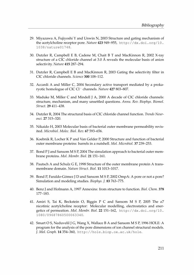
Bibliography
29. Miyazawa A, Fujiyoshi Y and Unwin N, 2003 Structure and gating mechanism ofthe acetylcholine receptor pore. Nature 423 949–955, http://dx.doi.org/10.1038/nature01748.
30. Dutzler R, Campbell E B, Cadene M, Chait B T and MacKinnon R, 2002 X-raystructure of a ClC chloride channel at 3.0 A reveals the molecular basis of anionselectivity. Nature 415 287–294.
31. Dutzler R, Campbell E B and MacKinnon R, 2003 Gating the selectivity filter inClC chloride channels. Science 300 108–112.
32. Accardi A and Miller C, 2004 Secondary active transport mediated by a proka-ryotic homologue of ClC Cl− channels. Nature 427 803–807.
33. Maduke M, Miller C and Mindell J A, 2000 A decade of ClC chloride channels:structure, mechanism, and many unsettled questions. Annu. Rev. Biophys. Biomol.Struct. 29 411–438.
34. Dutzler R, 2004 The structural basis of ClC chloride channel function. Trends Neur-osci. 27 315–320.
35. Nikaido H, 2003 Molecular basis of bacterial outer membrane permeability revis-ited. Microbiol. Molec. Biol. Rev. 67 593–656.
36. Koebnik R, Locher K P and Van Gelder P, 2000 Structure and function of bacterialouter membrane proteins: barrels in a nutshell. Mol. Microbiol. 37 239–253.
37. Bond P J and Sansom M S P, 2004 The simulation approach to bacterial outer mem-brane proteins. Mol. Membr. Biol. 21 151–161.
38. Pautsch A and Schulz G E, 1998 Structure of the outer membrane protein A trans-membrane domain. Nature Struct. Biol. 11 1013–1017.
39. Bond P, Faraldo-Gomez J D and Sansom M S P, 2002 OmpA: A pore or not a pore?Simulation and modeling studies. Biophys. J. 83 763–775.
40. Benz J and Hofmann A, 1997 Annexins: from structure to function. Biol. Chem. 378177–183.
41. Amiri S, Tai K, Beckstein O, Biggin P C and Sansom M S P, 2005 The α7nicotinic acetylcholine receptor: Molecular modelling, electrostatics and ener-getics of permeation. Mol. Membr. Biol. 22 151–162, http://dx.doi.org/10.1080/09687860500063340.
42. Smart O S, Neduvelil J G, Wang X, Wallace B A and Sansom M S P, 1996 HOLE: Aprogram for the analysis of the pore dimensions of ion channel structural models.J. Mol. Graph. 14 354–360, http://hole.biop.ox.ac.uk/hole.
211
Bibliography
43. Humphrey W, Dalke A and Schulten K, 1996 VMD – Visual Molecular Dynamics.J. Mol. Graph. 14 33–38, http://www.ks.uiuc.edu/Research/vmd/.
44. Merritt E A and Bacon D J, 1997 Raster3D: Photorealistic molecular graphics. Meth-ods Enzymol. 277 505–524, http://www.bmsc.washington.edu/raster3d/raster3d.html.
45. Spencer R H and Rees D C, 2002 The α-helix and the organization and gating ofchannels. Annu. Rev. Biophys. Biomol. Struct. 31 207–233.
46. Betanzos M, Chiang C S, Guy H R and Sukharev S, 2002 A large iris-like expan-sion of a mechanosensitive channel protein induced by membrane tension. NatureStruct. Biol. 9 704–710.
47. Eisenberg D and Kauzmann W, 1969 The Structure and Properties of Water (OxfordUniversity Press, London).
48. Kuo A, Gulbis J M, Antcliff J F, Rahman T, Lowe E D, Zimmer J, Cuthbertson J,Ashcroft F M, Ezaki T and Doyle D A, 2003 Crystal structure of the potassiumchannel KirBac1.1 in the closed state. Science 300 1922–1926.
49. Morais-Cabral J H, Zhou Y and MacKinnon R, 2001 Energetic optimization of ionconduction rate by the K+ selectivity filter. Nature 414 37–42.
50. Biggin P C and Sansom M S P, 2002 Open-state models of a potassium channel.Biophys. J. 83 1867–1876.
51. Chang G, Spencer R H, Lee A T, Barclay M T and Rees D C, 1998 Structure ofthe MscL homolog from Mycobacterium tubercolosis: a gated mechanosensitive ionchannel. Science 282 2220–2226.
52. Yoshimura K, Batiza A, Schroeder M, Blount P and Kung C, 1999 Hydrophilicityof a single residue within MscL correlates with increased channel mechanosensit-ivity. Biophys. J. 77 1960–1972.
53. Yoshimura K, Batiza A and Kung C, 2001 Chemically charging the pore constric-tion opens the mechanosensitive channel MscL. Biophys. J. 80 2198–2206.
54. Sukharev S, Betanzos M, Chiang C S and Guy H R, 2001 The gating mechanism ofthe large mechanosensitive channel MscL. Nature 409 720–724.
55. Bass R B, Strop P, Barclay M and Rees D C, 2002 Crystal structure of Escherichia coliMscS, a voltage-modulated and mechanosensitive channel. Science 298 1582–1587.
56. Anishkin A and Sukharev S, 2004 Water dynamics and dewetting transitions inthe small mechanosensitive channel MscS. Biophys. J. 86 2883–2895.
212

Bibliography
57. Perozo E, Kloda A, Cortes D M and Martinac B, 2002 Physical principles underly-ing the transduction of bilayer deformation forces during mechanosensitive chan-nel gating. Nature Struct. Biol. 9 696–703.
58. Unwin N, 1995 Acetylcholine-receptor channel imaged in the open state. Nature373 37–43.
59. Unwin N, 2000 The Croonian Lecture 2000. Nicotinic acetylcholine receptor andthe structural basis of fast synaptic transmission. Phil. Trans. Roy. Soc. London B 3551813–1829.
60. Unwin N, Miyazawa A, Li J and Fujiyoshi Y, 2002 Activation of the nicotinic acet-ylcholine receptor involves a switch in conformation of the alpha subunits. J. Mol.Biol. 319 1165–1176.
61. Unwin N, 2003 Structure and action of the nicotinic acetylcholine receptor ex-plored by electron microscopy. FEBS Lett. 555 91–95.
62. Beckstein O, Biggin P C and Sansom M S P, 2001 A hydrophobic gating mechan-ism for nanopores. J. Phys. Chem. B 105 12902–12905, http://dx.doi.org/10.1021/jp012233y.
63. Parsegian A, 1969 Energy of an ion crossing a low dielectric membrane: solutionto four relevant electrostatic problems. Nature 221 844–846.
64. Chung S H, Hoyles M, Allen T and Kuyucak S, 1998 Study of ionic currents acrossa model membrane channel using brownian dynamics. Biophys. J. 75 793–809.
65. Unwin N, 1993 Nicotinic acetylcholine-receptor at 9 A resolution. J. Mol. Biol. 2291101–1124.
66. Moe P C, Levin G and Blount P, 2000 Correlating a protein structure with functionof a bacterial mechanosensitive channel. J. Biol. Chem. 275 31121–31127.
67. Kipling R, 1902 Just So Stories (Project Gutenberg), http://www.gutenberg.org/dirs/etext01/jusss10.txt, print edition published in 1902, accessedonline October 2004.
68. Stroud R M, Miercke L J W, Connell J O, Khademi S, Lee J K, Remis J, HarriesW, Robles Y and Akhavan D, 2003 Glycerol facilitator GlpF and the associatedaquaporin family of channels. Curr. Opin. Struct. Biol. 13 424–431.
69. Sui H, Han B G, Lee J K, Walian P and Jap B K, 2001 Structural basis of water-specific transport through the AQP1 water channel. Nature 414 872–878.
70. Savage D F, Egea P F, Robles-Colmenares Y, O’Connell III J D and Stroud R M, 2003Architecture and selectivity in aquaporins: 2.5 A X-ray structure of aquaporin Z.PLoS Biol. 1 334–340.
213
Bibliography
71. Fu D, Libson A, Miercke L J, Weitzman C, Nollert P, Krucinski J and Stroud R M,2000 Structure of a glycerol-conducting channel and the basis for its selectivity.Science 290 481–486.
72. Tajkhorshid E, Nollert P, Jensen M Ø, Miercke L J, O’Connell J, Stroud R M andSchulten K, 2002 Control of the selectivity of the aquaporin water channel familyby global orientational tuning. Science 296 525–530.
73. Tournaire-Roux C, Sutka M, Javot H, Gout E, Gerbeau P, Luu D T, Bligny R andMaurel C, 2003 Cytosolic pH regulates root water transport during anoxic stressthrough gating of aquaporins. Nature 425 393–397.
74. Gonen T, Sliz P, Kistler J, Cheng Y and Walz T, 2004 Aquaporin-0 membrane junc-tions reveal the structure of a closed water pore. Nature 429 193–197.
75. Khademi S, O’Connell Joseph I, Remis J, Robles-Colmenares Y, Miercke L J W andStroud R M, 2004 Mechanism of ammonia transport by Amt/MEP/Rh: Structureof AmtB at 1.35 A. Science 305 1587–1594.
76. Raushel F M, Thoden J B and Holden H M, 2003 Enzymes with molecular tunnels.Acc. Chem. Res. 36 539–548.
77. Hyde C C, Ahmed S A, Padlan E A, Miles E W and Davies D R, 1988 Three-dimensional structure of the tryptophan synthase α2β2 multienzyme complexfrom Salmonella typhimurium. J. Biol. Chem. 263 17857–17871.
78. Binda C, Bossi R T, Wakatsuki S, Arzt S, Coda A, Curti B, Vanoni M A and MatteviA, 2000 Cross-talk and ammonia channeling between active centers in the unex-pected domain arrangement of glutamate synthase. Structure 8 1299–1308.
79. Doukov T I, Iverson T M, Seravalli J, Ragsdale S W and Drennan C L, 2002 ANi-Fe-Cu center in a bifunctional carbon monoxide dehydrogenase/acetyl-CoAsynthase. Science 298 567–572.
80. Darnault C, Volbeda A, Kim E J, Legrand P, Vernede X, Lindahl P A and Fontecilla-Camps J C, 2003 Ni-Zn-[Fe4-S4] and Ni-Ni-[Fe4-S4] clusters in closed and open αsubunits of acetyl-CoA synthase/carbon monoxide dehydrogenase. Nature Struct.Biol. 10 271–279.
81. Montet Y, Amara P, Volbeda A, Vernede X, Hatchikian E C, J. F M, M. F andFontecilla-Camps J C, 1997 Gas access to the active site of Ni-Fe hydrogenasesprobed by X-ray crystallography and molecular dynamics. Nature Struct. Biol. 4523–526.
82. Dill K A and Bromberg S, 2003 Molecular Driving Forces (Garland Science, NewYork).
214
Bibliography
83. Lazaridis T, 2001 Solvent size vs cohesive energy as the origin of hydrophobicity.Acc. Chem. Res. 34 931–937.
84. Pratt L R and Pohorille A, 2002 Hydrophobic effects and modeling of biophysicalaqueous solution interfaces. Chem. Rev. 102 2671–2692.
85. Chandler D, 2002 Two faces of water. Nature 417 491.
86. Hummer G, Garde S, Garcıa A E, Paulaitis M E and Pratt L R, 1998 Hydrophobiceffects on a molecular scale. J. Phys. Chem. B 102 10469–10482.
87. Jorgensen W L, Gao J and Ravimohan C, 1985 Monte carlo simulations of alkanesin water: hydration numbers and the hydrophobic effect. J. Phys. Chem. 89 3470–3473.
88. Humphrey W, Dalke A and Schulten K, 1996 VMD – Visual Molecular Dynamics.J. Mol. Graph. 14 33–38, http://www.ks.uiuc.edu/Research/vmd/.
89. Wallqvist A and Berne B J, 1995 Computer simulation of hydrophobic hydrationforces on stacked plates at short range. J. Phys. Chem. 99 2893.
90. Lum K, Chandler D and Weeks J D, 1999 Hydrophobicity at small and large lengthscales. J. Phys. Chem. B 103 4570–4577.
91. Huang D M and Chandler D, 2000 Temperature and length scale dependence ofhydrophobic effects and their possible implications for protein folding. Proc. Natl.Acad. Sci. U.S.A. 97 8324–8327.
92. de Gennes P G, 1985 Wetting: statics and dynamics. Rev. Mod. Phys. 57 827–863.
93. Stillinger F H, 1973 Structure in aqueous solutions of nonpolar solutes from thestandpoint of scaled particle theory. J. Solution Chem. 2 141–158.
94. Huang X, Margulis C J and Berne B J, 2003 Dewetting-induced collapse of hydro-phobic particles. Proc. Natl. Acad. Sci. U.S.A. 100 11953–11958.
95. Tieleman D P, Biggin P C, Smith G R and Sansom M S P, 2001 Simulation ap-proaches to ion channel structure-function relationships. Quart. Rev. Biophys. 34473–561.
96. Beckstein O and Sansom M S P, 2003 Liquid-vapor oscillations of water in hy-drophobic nanopores. Proc. Natl. Acad. Sci. U.S.A. 100 7063–7068, http://www.pnas.org/cgi/content/abstract/100/12/7063.
97. Beckstein O and Sansom M S P, 2004 The influence of geometry, surface charac-ter, and flexibility on the permeation of ions and water through biological pores.Physical Biology 1 42–52, http://stacks.iop.org/1478-3975/1/42.
215
Bibliography
98. Beckstein O, Tai K and Sansom M S P, 2004 Not ions alone: Barriers to ion per-meation in nanopores and channels. J. Am. Chem. Soc. 126 14694–14695, http://dx.doi.org/10.1021/ja045271e.
99. Chaikin P M and Lubensky T C, 2000 Principles of condensed matter physics (Cam-bridge University Press, Cambridge).
100. Rowlinson J S and Widom B, 2002 Molecular Theory of Capillarity (Dover Publica-tions, Mineola, New York), reprint of Ref. 231.
101. Hansen J P and McDonald I R, 1990 Theory of Simple Liquids, 2nd edn. (ElsevierAcademic Press, Amsterdam).
102. van Swol F and Henderson J R, 1986 Wetting at a fluid-wall interface. J. Chem. Soc.,Faraday Trans. 2 82 1685–1699.
103. van Swol F and Henderson J R, 1989 Wetting and drying transitions at a fluid-wallinterface: Density-functional theory versus computer simulation. Phys. Rev. A 402567–2578.
104. Nijmeijer M J P, Bruin C, Bakker A F and van Leeuwen J M J, 1991 Determina-tion of the location and order of the drying transition with a molecular dynamicssimulation. Phys. Rev. B 44 834–837.
105. Allen M P and Tildesley D J, 1987 Computer Simulations of Liquids (Oxford Univer-sity Press, Oxford).
106. McQuarrie D A, 1976 Statistical Mechanics (HarperCollins, New York).
107. Deutsch D, 1997 The Fabric of Reality (Penguin Books, London).
108. Huang K, 1987 Statistical Mechanics, 2nd edn. (John Wiley & Sons, New York).
109. Tegmark M, Strauss M A, Blanton M R, Abazajian K, Dodelson S, Sandvik H,Wang X, Weinberg D H, Zehavi I, Bahcall N A, Hoyle F, Schlegel D, ScoccimarroR, Vogeley M S, Berlind A, Budavari T, Connolly A, Eisenstein D J, FinkbeinerD, Frieman J A, Gunn J E, Hui L, Jain B, Johnston D, Kent S, Lin H, NakajimaR, Nichol R C, Ostriker J P, Pope A, Scranton R, Seljak U, Sheth R K, Stebbins A,Szalay A S, Szapudi I, Xu Y, Annis J, Brinkmann J, Burles S, Castander F J, CsabaiI, Loveday J, Doi M, Fukugita M, Gillespie B, Hennessy G, Hogg D W, Ivezic Z,Knapp G R, Lamb D Q, Lee B C, Lupton R H, McKay T A, Kunszt P, Munn J A,O’Connell L, Peoples J, Pier J R, Richmond M, Rockosi C, Schneider D P, StoughtonC, Tucker D L, Berk D E V, Yanny B and York D G, 2004 Cosmological parametersfrom SDSS and WMAP. Phys. Rev. D 69 103501.
110. Zwanzig R and Ailawadi N K, 1969 Statistical error due to finite time averagingin computer experiments. Phys. Rev. 182 280–283.
216

Bibliography
111. Chandrasekhar S, 1943 Stochastic problems in physics and astronomy.Rev. Mod. Phys. 15 1–89.
112. Einstein A, 1905 Uber die von der molekularkinetischen Theorie der Warmegeforderte Bewegung von in ruhenden Flussigkeiten suspendierten Teilchen.Ann. d. Phys. 17 549–560.
113. Adamson A W, 1990 Physical Chemistry of Surfaces, 5th edn. (John Wiley & Sons,Inc, New York).
114. Rowlinson J S, 1986 The statistical mechanics of small systems. J. Chem. Soc.,Faraday Trans. 2 82 1801–1815, Faraday Symposium 20, The Lennard-Jones Lec-ture.
115. Barrat J L and Hansen J P, 2003 Basic Concepts for Simple and Complex Liquids (Cam-bridge University Press, Cambridge).
116. Chalikian T V, 2003 Volumetric properties of proteins. Annu. Rev. Biophys. Biomol.Struct. 32 207–235.
117. Richards F M, 1977 Areas, volumes, packing and protein structure. Annu. Rev.Biophys. Bioeng. 6 151–176.
118. Connolly M L, 1983 Solvent-accessible surfaces of proteins and nucleic-acids. Sci-ence 221 709–713.
119. Connolly M L, 1985 Computation of molecular volume. J. Am. Chem. Soc. 107 1118–1124.
120. Lee B and Richards F M, 1971 The interpretation of protein structures: estimationof static accessibility. J. Mol. Biol. 55 379–400.
121. Sanner M F, Olson A J and Spehner J C, 1996 Reduced surface: An efficient way tocompute molecular surfaces. Biopolymers 38 305–320.
122. Greer J and Bush B L, 1978 Macromolecular shape and surface maps by solventexclusion. Proc. Natl. Acad. Sci. U.S.A. 75 303–307.
123. Weeks J D, Chandler D and Andersen H C, 1971 Role of repulsive forces in de-termining the equilibrium structure of simple liquids. J. Chem. Phys. 54 5237–5247.
124. Born M and Oppenheimer R, 1927 Zur Quantentheorie der Molekeln. Ann. d. Phys.84 457–484.
125. Schwabl F, 1993 Quantenmechanik, 4th edn. (Springer, Heidelberg).
126. Goldstein H, 1980 Classical Mechanics, 2nd edn. (Addison-Wesley, Reading, Mas-sachusetts).
217

Bibliography
127. Lindahl E, Hess B and van der Spoel D, 2001 Gromacs 3.0: A package for mo-lecular simulation and trajectory analysis. J. Mol. Mod. 7 306–317, http://www.gromacs.org.
128. Berendsen H J C, van der Spoel D and van Drunen R, 1995 GROMACS: A message-passing parallel molecular dynamics implementation. Comp. Phys. Comm. 91 43–56.
129. van der Spoel D, Lindahl E, Hess B, van Buuren A R, Apol E, Meulenhoff P J,Tieleman D P, M.Sijbers A L T, Feenstra K A, van Drunen R and Berendsen H J C,2004 Gromacs User Manual version 3.2, The Gromacs development team, http://www.gromacs.org.
130. Harding J, Heyes D M, Smith W, Howlin B, Anwar J, Wilding N, Refson K andLindan P, 2002 The CCP5 molecular simulation summer school 2002, King’s Col-lege, London.
131. Mackerell A D, 2004 Empirical force fields for biological macromolecules: Over-view and issues. J. Comp. Chem. 25 1584–1604.
132. Hermans J, Berendsen H J C, van Gunsteren W F and Postma J P M, 1984 A consist-ent empirical potential for water-protein interactions. Biopolymers 23 1513–1518.
133. van Gunsteren W F, Billeter S R, Elsing A A, Hunenberger P H, Kruger P, Mark A E,Scott W R P and Tironi I G, 1996 Biomolecular Simulation: The GROMOS96 Manualand User Guide, Biomos and Hochschulverlag AG an der ETH Zurich, Zurich andGroningen.
134. Jorgensen W L, Maxwell D S and Tirado-Rives J, 1996 Development and testingof the OPLS all-atom force field on conformational energetics and properties oforganic liquids. J. Am. Chem. Soc. 118 11225–11236.
135. McDonald N A and Jorgensen W L, 1998 Development of an all-atom forcefield for heterocycles. properties of liquid pyrrole, furan, diazoles, and oxazoles.J. Phys. Chem. B 102 8049–8059.
136. McDonald N A and Jorgensen W L, 1998 Development of an all-atom forcefield for heterocycles. properties of liquid pyridine and diazenes. Theochem.J. Mol. Struc. 424 145–155.
137. Rizzo R C and Jorgensen W L, 1999 OPLS all-atom model for amines: Resolutionof the amine hydration problem. J. Am. Chem. Soc. 121 4827–4836.
138. Price M L P, Ostrovsky D and Jorgensen W L, 2001 Gas-phase and liquid-stateproperties of esters, nitriles, and nitro compounds with the OPLS-AA force field.J. Comp. Chem. 22 1340–1352.
218
Bibliography
139. Watkins E K and Jorgensen W L, 2001 Perfluoroalkanes: Conformational ana-lysis and liquid-state properties from ab initio and Monte Carlo calculations.J. Phys. Chem. A 105 4118–4125.
140. Kaminski G A, Friesner R A, Tirado-Rives J and Jorgensen W L, 2001 Evaluationand reparametrization of the OPLS-AA force field for proteins via comparisonwith accurate quantum chemical calculations on peptides. J. Phys. Chem. B 1056474–6487.
141. Jorgensen W L and Jenson C, 1998 Temperature dependence of TIP3P, SPC, andTIP4P water from NPT Monte Carlo simulations: Seeking temperatures of max-imum density. J. Comp. Chem. 19 1179–1186.
142. van der Spoel D and Lindahl E, 2003 Brute-force molecular dynamics simula-tions of Villin headpiece: Comparison with NMR parameters. J. Phys. Chem. B107 11178–11187.
143. Berendsen H J C, Postma J P M, van Gunsteren W F and Hermans J, 1981 Inter-action models for water in relation to protein hydration, in Intermolecular Forces(edited by B Pullman), 331 (D. Reidel Publishing Company, Dordrecht, Holland).
144. Jorgensen W L, Chandrasekhar J, Madura J D, Impey R W and Klein M L,1983 Comparison of simple potential functions for simulating liquid water.J. Chem. Phys. 79 926–935.
145. Jorgensen W L and Madura J D, 1985 Temperature and size dependence for Monte-Carlo simulations of TIP4P water. Mol. Phys. 56 1381–1392.
146. van der Spoel D, van Maaren P J and Berendsen H J C, 1998 A systematic studyof water models for molecular simulation: Derivation of water models optimizedfor use with a reaction field. J. Chem. Phys. 108 10220–10230.
147. Mark P and Nilsson L, 2001 Structure and dynamics of the TIP3P, SPC, and SPC/Ewater models at 298 K. J. Phys. Chem. A 105 9954–9960.
148. Guillot B, 2002 A reappraisal of what we have learnt during three decades of com-puter simulations on water. J. Mol. Liquids 101 219–260.
149. Aqvist J, 1990 Ion-water interaction potentials derived from free energy perturba-tion simulations. J. Phys. Chem. 94 8021–8024.
150. Chandrasekhar J, Spellmeyer D C and Jorgensen W L, 1984 Energy compon-ent analysis for dilute aqueous solutions of Li+, Na+, F−, and Cl− ions.J. Am. Chem. Soc. 106 903–910.
151. Marcus Y, 1988 Ionic radii in aqueous solutions. Chem. Rev. 88 1475–1473.
219

Bibliography
152. Verlet L, 1967 Computer “experiments” on classical fluids. I. Thermodynamicalproperties of Lennard-Jones molecules. Phys. Rev. 159 98–103.
153. Frenkel D and Smit B, 2002 Understanding Molecular Simulations, 2nd edn. (Aca-demic Press, San Diego).
154. Hockney R W, Goel S P and Eastwood J W, 1974 Quiet high-resolution computermodels of a plasma. J. Comp. Phys. 14 148–158.
155. Hess B, Bekker H, Berendsen H J C and Fraaije J G E M, 1997 LINCS: A linearconstraint solver for molecular simulations. J. Comp. Chem. 18 1463–1472.
156. Ryckaert J P, Ciccotti G and Berendsen H J C, 1977 Numerical integration of thecartesian equations of motion of a system with constraints; molecular dynamicsof n-alkanes. J. Comp. Phys. 23 327–341.
157. Miyamoto S and Kollman P A, 1992 SETTLE: An analytical version of the SHAKEand RATTLE algorithms for rigid water models. J. Comp. Chem. 13 952–962.
158. Darden T A, 2001 Treatment of long-range forces and potential, in ComputationalBiochemistry and Biophysics (edited by O M Becker, J Alexander D. Mackerell,B Roux and M Watanabe), 91–114 (Marcel Dekker, Inc., New York).
159. Feller S E, Pastor R W, Rojnuckarin A, Bogusz S and Brooks B R, 1996 Effectof electrostatic force truncation on interfacial and transport properties of water.J. Phys. Chem. A 100 17011–17020.
160. Ewald P P, 1921 Die Berechnung optischer und elektrostatischer Gitterpotentiale.Ann. d. Phys. 64 253–287.
161. Deserno M and Holm C, 1998 How to mesh up Ewald sums. I. A theoretical andnumerical comparison of various particle mesh routines. J. Chem. Phys. 109 7678–7693.
162. Press W H, Teukolsky S A, Vetterling W T and Flannery B P, 1992 Numerical Re-cipes in C, 2nd edn. (Cambridge University Press, Cambridge), http://www.library.cornell.edu/nr/bookcpdf.html.
163. Hockney R W and Eastwood J W, 1988 Computer Simulation Using Particles (Insti-tute of Physics, Bristol).
164. Darden T, York D and Pedersen L, 1993 Particle mesh Ewald – an N log(N)method for Ewald sums in large systems. J. Chem. Phys. 98 10089–10092.
165. Essman U, Perela L, Berkowitz M L, Darden T, Lee H and Pedersen L G, 1995 Asmooth particle mesh Ewald method. J. Chem. Phys. 103 8577–8592.
166. Berendsen H J C, Postma J P M, DiNola A and Haak J R, 1984 Molecular dynamicswith coupling to an external bath. J. Chem. Phys. 81 3684–3690.
220

Bibliography
167. Harvey S C, Tan R K Z and Cheatham T E, 1998 The flying ice cube: Velo-city rescaling in molecular dynamics leads to violation of energy equipartition.J. Comp. Chem. 19 726–740.
168. Kirkwood J G, 1935 Statistical mechanism of fluid mixtures. J. Chem. Phys. 3 300–313.
169. Roux B, Allen T, Berneche S and Im W, 2004 Theoretical and computational modelsof biological ion channels. Quart. Rev. Biophys. 37 15–103.
170. Allen T W, Andersen O S and Roux B, 2004 Energetics of ion conduction throughthe gramicidin channel. Proc. Natl. Acad. Sci. U.S.A. 101 117–122.
171. Smith G R and Sansom M S, 2002 Free energy of a potassium ion in a model ofthe channel formed by an amphipathic leucine-serine peptide. Eur. Biophys. J. 31198–206.
172. Valleau J P and Torrie G M, 1977 A guide to Monte Carlo for statistical mechanics:2. Byways, in Statistical Mechanics. Part A: Equilibrium Techniques (edited by B JBerne), vol. 5 of Modern Theoretical Chemistry, chap. 5, 169–194 (Plenum Press, NewYork).
173. Torrie G M and Valleau J P, 1977 Nonphysical sampling distributions in MonteCarlo free-energy estimation: Umbrella sampling. J. Comp. Phys. 23 187–199.
174. Roux B, 1995 The calculation of the potential of mean force using computer simu-lations. Comp. Phys. Comm. 91 275–282.
175. Kumar S, Bouzida D, Swendsen R H, Kollman P A and Rosenberg J M, 1992The Weighted Histogram Analysis Method for free-energy calculations on bio-molecules. I. The method. J. Comp. Chem. 13 1011–1021.
176. Roux B and Karplus M, 1991 Ion transport in a model gramicidin channel: Struc-ture and thermodynamics. Biophys. J. 59 961–981.
177. Debye P and Huckel E, 1923 Zur Theorie der Elektrolyte. I. Gefrierpunktserniedri-gung und verwandte Erscheinungen. Phys. Z. 24 185–206.
178. Honig B and Nicholls A, 1995 Classical electrostatics in biology and chemistry.Science 268 1144–1149.
179. Baker N A, Sept D, Joseph S, Holst M J and McCammon J A, 2001 Electrostatics ofnanosystems: application to microtubules and the ribosome. Proc. Natl. Acad. Sci.U.S.A. 98 10037–10041, http://agave.wustl.edu/apbs/.
180. Sharp K A and Honig B, 1990 Calculating total electrostatic energies with the non-linear Poisson-Boltzmann equation. J. Phys. Chem. 94 7684–7692.
221
Bibliography
181. Rashin A A and Honig B, 1985 Reevaluation of the Born model of ion hydration.J. Phys. Chem. 89 5588–5593.
182. Holst M, Baker N and Wang F, 2000 Adaptive multilevel finite element solutionof the Poisson-Boltzmann equation I. Algorithms and examples. J. Comp. Chem. 211319–1342.
183. Baker N, Holst M and Wang F, 2000 Adaptive multilevel finite element solutionof the Poisson-Boltzmann equation II. Refinement at solvent-accessible surfaces inbiomolecular systems. J. Comp. Chem. 21 1343–1352.
184. Nielsen J E and McCammon J A, 2003 Calculating pKa values in enzyme activesites. Protein Sci. 12 1894–1901, http://enzyme.ucd.ie/Science/pKa/.
185. Nielsen J E and Vriend G, 2001 Optimizing the hydrogen-bond network inPoisson-Boltzmann equation-based pKa calculations. Proteins: Struct. Funct. Genet.43 403–412.
186. Rocchia W, Alexov E and Honig B, 2001 Extending the applicability of the non-linear Poisson-Boltzmann equation: Multiple dielectric constants and multivalentions. J. Phys. Chem. B 105 6507–6514, http://trantor.bioc.columbia.edu/delphi/.
187. Yang B, van Hoek A N and Verkman A S, 1997 Very high single channel waterpermeability of aquaporin-4 in baculovirus-infected insect cells and liposomes re-constituted with purified aquaporin-4. Biochemistry 36 7625–7632.
188. Pohl P, Saparov S M, Borgnia M J and Agre P, 2001 Highly selective water channelactivity measured by voltage clamp: analysis of planar lipid bilayers reconstitutedwith purified AqpZ. Proc. Natl. Acad. Sci. U.S.A. 98 9624–9629.
189. Pohl P and Saparov S M, 2000 Solvent drag across gramicidin channels demon-strated by microelectrodes. Biophys. J. 78 2426–2434.
190. Saparov S M, Antonenko Y N, and Pohl P, 2000 Desformylgramicidin: a modelchannel with an extremely high water permeability. Biophys. J. 79 2526–2534.
191. de Groot B L, Tieleman D P, Pohl P and Grubmuller H, 2002 Water permeationthrough gramicidin A: desformylation and the double helix: a molecular dynam-ics study. Biophys. J. 82 2934–2942.
192. de Groot B L and Grubmuller H, 2001 Water permeation across biological mem-branes: Mechanism and dynamics of aquaporin-1 and GlpF. Science 294 2353–2357.
193. Christenson H K, 2001 Confinement effects on freezing and melting. J. Phys.: Con-dens. Matter 13 R95–R133.
222
Bibliography
194. Gelb L D, Gubbins K E, Radhakrishnan R and Sliwinska-Bartkowiak M, 1999Phase separation in confined systems. Rep. Prog. Phys. 62 1573–1659.
195. Lynden-Bell R M and Rasaiah J C, 1996 Mobility and solvation of ions in channels.J. Chem. Phys. 105 9266–9280.
196. Allen T W, Kuyucak S and Chung S H, 1999 The effect of hydrophobic and hydro-philic channel walls on the structure and diffusion of water and ions. J. Chem. Phys.111 7985–7999.
197. Hummer G, Rasaiah J C and Noworyta J P, 2001 Water conduction through thehydrophobic channel of a carbon nanotube. Nature 414 188–190.
198. Allen R, Melchionna S and Hansen J P, 2002 Intermittent permeation of cylindricalnanopores by water. Phys. Rev. Lett. 89 175502.
199. Brovchenko I and Geiger A, 2002 Water in nanopores in equilibrium with a bulkreservoir—Gibbs ensemble Monte Carlo simulations. J. Mol. Liquids 96–97 195–206.
200. Ashcroft N W and Mermin N D, 1976 Solid State Physics (Saunders College Pub-lishing, Fort Worth).
201. Domene C, Grottesi A and Sansom M S P, 2004 Filter flexibility and distortion in abacterial inward rectifier K+ channel: Simulation studies of KirBac1.1. Biophys. J.87 256–267.
202. Allen R, Hansen J P and Melchionna S, 2003 Molecular dynamics investigation ofwater permeation through nanopores. J. Chem. Phys. 119 3905–3919.
203. Hunter III J E and Reinhardt W P, 1995 Finite-size scaling behavior of the free en-ergy barrier between coexisting phases: Determination of the critical temperatureand interfacial tension of the Lennard-Jones fluid. J. Chem. Phys. 103 8627–8637.
204. Sakmann B and Neher E, eds., 1983 Single-Channel Recordings (Plenum Press, NewYork).
205. Flyvbjerg H and Petersen H G, 1989 Error estimates on averages of correlated data.J. Chem. Phys. 91 461–466.
206. Hess B, 1999 Stochastic concepts in molecular simulation, Ph.D. thesis, Rijk-suniversiteit Groningen, Groningen, http://www.ub.rug.nl/eldoc/dis/science/b.hess/.
207. Evans R, 1990 Fluids adsorbed in narrow pores: phase equilibria and structure.J. Phys.: Condens. Matter 2 8989–9007.
208. Lee C Y, McCammon J A and Rossky P J, 1984 The structure of liquid water at anextended hydrophobic surface. J. Chem. Phys. 80 4448–4455, http://link.aip.org/link/?JCP/80/4448/1.
223

Bibliography
209. Lee S H and Rossky P J, 1994 A comparison of the structure and dynamics of li-quid water at hydrophobic and hydrophilic surfaces—a molecular dynamics sim-ulation study. J. Chem. Phys. 100 3334–3345.
210. Spohr E, Trokhymchuk A and Henderson D, 1998 Adsorption of water moleculesin slit pores. J. Electroanalyt. Chem. 450 281–287.
211. Gallo P, Rovere M and Spohr E, 2000 Glass transition and layering effects in con-fined water: A computer simulation study. J. Chem. Phys. 113 11324–11335.
212. Freund J B, 2002 Electro-osmosis in a nanometer-scale channel studied by atom-istic simulation. J. Chem. Phys. 116 2194–2200.
213. Striolo A, Chiavolo A A, Cummings P T and Gubbins K E, 2003 Water adsorptionin carbon-slit nanopores. Langmuir 19 8583–8591.
214. Kalra A, Garde S and Hummer G, 2003 Osmotic water transport through carbonnanotube membranes. Proc. Natl. Acad. Sci. U.S.A. 100 10175–10180.
215. Jensen M Ø, Mouritsen O G and Peters G H, 2004 The hydrophobic effect: Mo-lecular dynamics simulations of water confined between extended hydrophobicand hydrophilic surfaces. J. Chem. Phys. 120 9729–9744.
216. Mamatkulov S I, Khabibullaev P K and Netz R R, 2004 Water at hydrophobic sub-strates: Curvature, pressure, and temperature effects. Langmuir 20 4756–4763.
217. Klein J and Kurnacheva E, 1998 Simple liquids confined to molecularly thin layers.I Confinement-induced liquid-to-solid phase transitions. J. Chem. Phys. 108 6996–7009.
218. Raviv U, Laurat P and Klein J, 2001 Fluidity of water confined to subnanometrefilms. Nature 413 51–54.
219. Dore J, 2000 Structural studies of water in confined geometry by neutron diffrac-tion. Chem. Phys. 258 327–347.
220. Wallqvist A, Gallicchio E and Levy R M, 2001 A model for studying drying at hy-drophobic interfaces: Structural and thermodynamic properties. J. Phys. Chem. B105 6745–6753.
221. Aarts D G A L, Schmidt M and Lekkerkerker H N W, 2004 Direct visual observa-tion of thermal capillary waves. Science 304 847–850.
222. Mecke K, 2004 Mikroskopische Kapillarwellen sichtbar gemacht. Physik Journal 319–20, see also Aarts et al.221.
223. Preusser A, 1989 Algorithm 671—FARB-E-2D: Fill Area with Bicubics onRectangles—A contour plot program. ACM Trans. Math. Softw. 15 79–89, http://www.fhi-berlin.mpg.de/grz/pub/xfarbe/.
224

Bibliography
224. Brovchenko I, Geiger A and Oleinikova A, 2001 Phase equilibria of water in cyl-indrical nanopores. Phys. Chem. Chem. Phys. 3 1567–1569.
225. Hummer G, Garde S, Garcıa A E, Pohorille A and Pratt L R, 1996 An informationtheory model of hydrophobic interactions. Proc. Natl. Acad. Sci. U.S.A. 93 8951–8955.
226. Waghe A, Rasaiah J C and Hummer G, 2002 Filling and emptying kinetics of car-bon nanotubes in water. J. Chem. Phys. 117 10789–10795.
227. Privman V and Fisher M E, 1983 Finite-size effects at first-order transitions.J. Stat. Phys. 33 385–417.
228. Peterson B K, Gubbins K E, Heffelfinger G S, Marconi U M B and van Smol F,1988 Lennard-Jones fluids in cylindrical pores: Nonlocal theory and computersimulation. J. Chem. Phys. 88 6487–6500.
229. Martı J and Gordillo M C, 2001 Temperature effects on the static and thermody-namic properties of liquid water inside nanotubes. Phys. Rev. E 64 021504.
230. Berezhkovskii A and Hummer G, 2002 Single-file transport of water moleculesthrough a carbon nanotube. Phys. Rev. Lett. 89 065403.
231. Rowlinson J S and Widom B, 1982 Molecular Theory of Capillarity, no. 8 in The In-ternational series of monographs on chemistry (Clarendon Press, Oxford).
232. Giaya A and Thompson R W, 2002 Water confined in cylindrical micropores.J. Chem. Phys. 117 3464–3475.
233. Dujardin E, Ebbesen T W, Hiura H and Tanigaki K, 1994 Capillarity and wettingof carbon nanotubes. Science 265 1850–1852.
234. Bekyarova E, Hanzawa Y, Kaneko K, Silvestre-Albero J, Sepulveda-Escribano A,Rodriguez-Reinoso F, Kasuya D, Yudasaka M and Iijima S, 2002 Cluster-mediatedfilling of water vapor in intratube and interstitial nanospaces of single-wall carbonnanohorns. Chem. Phys. Lett. 366 463–468.
235. Naguib N, Ye H, Gogotsi Y, Yazicioglu A G, Megaridis C M and Yoshimura M, 2004Observation of water confined in nanometer channels of closed carbon nanotubes.Nano Lett. 4 2237–2243.
236. Allen R, Melchionna S and Hansen J P, 2003 Permeation of nanopores by water:the effects of channel polarization. J. Phys.: Condens. Matter 15 S297–S302.
237. Jiang Y, Lee A, Chen J, Ruta V, Cadene M, Chait B T and MacKinnon R, 2003 X-raystructure of a voltage-dependent K+ channel. Nature 423 33–41.
225
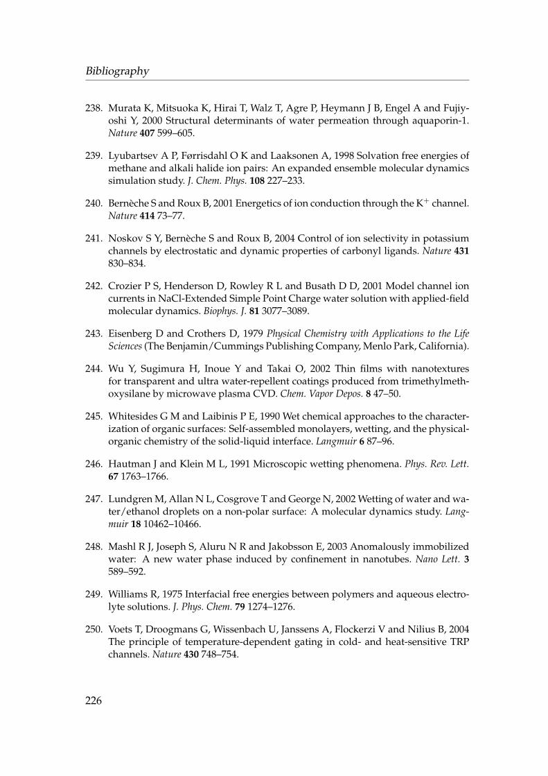
Bibliography
238. Murata K, Mitsuoka K, Hirai T, Walz T, Agre P, Heymann J B, Engel A and Fujiy-oshi Y, 2000 Structural determinants of water permeation through aquaporin-1.Nature 407 599–605.
239. Lyubartsev A P, Førrisdahl O K and Laaksonen A, 1998 Solvation free energies ofmethane and alkali halide ion pairs: An expanded ensemble molecular dynamicssimulation study. J. Chem. Phys. 108 227–233.
240. Berneche S and Roux B, 2001 Energetics of ion conduction through the K+ channel.Nature 414 73–77.
241. Noskov S Y, Berneche S and Roux B, 2004 Control of ion selectivity in potassiumchannels by electrostatic and dynamic properties of carbonyl ligands. Nature 431830–834.
242. Crozier P S, Henderson D, Rowley R L and Busath D D, 2001 Model channel ioncurrents in NaCl-Extended Simple Point Charge water solution with applied-fieldmolecular dynamics. Biophys. J. 81 3077–3089.
243. Eisenberg D and Crothers D, 1979 Physical Chemistry with Applications to the LifeSciences (The Benjamin/Cummings Publishing Company, Menlo Park, California).
244. Wu Y, Sugimura H, Inoue Y and Takai O, 2002 Thin films with nanotexturesfor transparent and ultra water-repellent coatings produced from trimethylmeth-oxysilane by microwave plasma CVD. Chem. Vapor Depos. 8 47–50.
245. Whitesides G M and Laibinis P E, 1990 Wet chemical approaches to the character-ization of organic surfaces: Self-assembled monolayers, wetting, and the physical-organic chemistry of the solid-liquid interface. Langmuir 6 87–96.
246. Hautman J and Klein M L, 1991 Microscopic wetting phenomena. Phys. Rev. Lett.67 1763–1766.
247. Lundgren M, Allan N L, Cosgrove T and George N, 2002 Wetting of water and wa-ter/ethanol droplets on a non-polar surface: A molecular dynamics study. Lang-muir 18 10462–10466.
248. Mashl R J, Joseph S, Aluru N R and Jakobsson E, 2003 Anomalously immobilizedwater: A new water phase induced by confinement in nanotubes. Nano Lett. 3589–592.
249. Williams R, 1975 Interfacial free energies between polymers and aqueous electro-lyte solutions. J. Phys. Chem. 79 1274–1276.
250. Voets T, Droogmans G, Wissenbach U, Janssens A, Flockerzi V and Nilius B, 2004The principle of temperature-dependent gating in cold- and heat-sensitive TRPchannels. Nature 430 748–754.
226

Bibliography
251. Beckstein O, Biggin P C, Bond P, Bright J N, Domene C, Grottesi A, Holyoake J andSansom M S P, 2003 Ion channel gating: insights via molecular simulations. FEBSLett. 555 85–90, http://dx.doi.org/10.1016/S0014-5793(03)01151-7.
252. Roosild T P, Miller S, Booth I R and Choe S, 2002 A mechanism of regulating trans-membrane potassium flux through a ligand-mediated conformational switch. Cell109 781–791.
253. McElroy C, Manfredo A, Wendt A, Gollnick P and Foster M, 2002 TROSY-NMRstudies of the 91 kDa TRAP protein reveal allosteric control of a gene regulatoryprotein by ligand-altered flexibility. J. Mol. Biol. 323 463–473.
254. Nicholls A, Sharp K A and Honig B, 1991 Protein folding and association: in-sights from the interfacial and thermodynamic properties of hydrocarbons. Pro-teins: Struct. Funct. Genet. 11 281–296.
255. Maibaum L and Chandler D, 2003 A coarse-grained model of water confined in ahydrophobic tube. J. Phys. Chem. B 107 1189–1193.
256. Harms G S, Orr G, Montal M, Thrall B D, Colson S D and Lu H P, 2003 Probing con-formational changes of gramicidin ion channels by single-molecule patch-clampfluorescence microscopy. Biophys. J. 85 1826–1838.
257. Goh C S, Milburn D and Gerstein M, 2004 Conformational changes associatedwith protein-protein interactions. Curr. Opin. Struct. Biol. 14 104–109.
258. Pang A, Arinaminpathy Y, Sansom M S P, and Biggin P C, 2003 Interdomain dy-namics and ligand binding: Molecular dynamics simulations of glutamine bind-ing protein. FEBS Lett. 550 168–174.
259. Hirama Y, Takahashi T, Hino M and Sato T, 1996 Studies of water adsorbed inporous vycor glass. J. Colloid Interface Sci. 184 349–359.
260. Koga K, Gao G, Tanaka H and Zeng X C, 2001 Formation of ordered ice nanotubesinside carbon nanotubes. Nature 412 802–805.
261. Levinger N E, 2002 Water in confinement. Science 298 1722–1723.
262. Weetman P, Goldman S and Gray C G, 1997 Use of the Poisson Boltzmann equa-tion to estimate the electrostatic free energy barrier for dielectric models of biolo-gical ion channels. J. Phys. Chem. B 101 6073–6078.
263. Corry B, Kuyucak S and Chung S H, 2000 Invalidity of continuum theories ofelectrolytes in nanopores. Chem. Phys. Lett. 320 35–41.
264. Edwards S, Corry B, Kuyucak S and Chung S H, 2002 Continuum electrostaticsfails to describe ion permeation in the gramicidin channel. Biophys. J. 83 1348–1360.
227
Bibliography
265. Miyazawa A, Fujiyoshi Y, Stowell M and Unwin N, 1999 Nicotinic acetylcholinereceptor at 4.6 A resolution: Transverse tunnels in the channel wall. J. Mol. Biol.288 765–786.
266. Wagner K, Edson K, Heginbotham L, Post M, Huganir R L and Czernik A J, 1991Determination of the tyrosine phosphorylation sites of the nicotinic acetylcholinereceptor. J. Biol. Chem. 266 23784–23789.
267. Mulder N J, Apweiler R, Attwood T K, Bairoch A, Barrell D, Bateman A, Binns D,Biswas M, Bradley P, Bork P, Bucher P, Copley R R, Courcelle E, Das U, DurbinR, Falquet L, Fleischmann W, Griffiths-Jones S, Haft D, Harte N, Hulo N, KahnD, Kanapin A, Krestyaninova M, Lopez R, Letunic I, Lonsdale D, Silventoinen V,Orchard S E, Pagni M, Peyruc D, Ponting C P, Selengut J D, Servant F, Sigrist C J,Vaughan R and Zdobnov E M, 2003 The InterPro database, 2003 brings increasedcoverage and new features. Nucleic Acids Res. 31 315–318, http://www.ebi.ac.uk/interpro/.
268. Kofuji P, Wang J B, Moss S J, Huganir R L and Burt D R, 1991 Generation of twoforms of the gamma-aminobutyric acid A receptor gamma 2-subunit in mice byalternative splicing. J. Neurochem. 56 713–715.
269. Sine S M, 2002 The nicotinic receptor ligand binding domain. J. Neurobiol. 53 431–446.
270. Bateman A, Coin L, Durbin R, Finn R D, Hollich V, Griffiths-Jones S, Khanna A,Marshall M, Moxon S, Sonnhammer E L, Studholme D J, Yeats C and Eddy S R,2004 The Pfam protein families database. Nucleic Acids Res. 32 D138–D141, http://www.sanger.ac.uk/Software/Pfam/.
271. Thompson J D, Higgins D G and Gibson T J, 1994 CLUSTAL W: improving thesensitivity of progressive multiple sequence alignment through sequence weight-ing, position-specific gap penalties and weight matrix choice. Nucleic Acids Res. 224673–4780.
272. Clamp M, Cuff J, Searle S M and Barton G J, 2004 The Jalview Java alignmenteditor. Bioinformatics 20 426–427, http://www.jalview.org.
273. Schneider T D and Stephens R M, 1990 Sequence logos: a new way to displayconsensus sequences. Nucleic Acids Res. 18 6097–6100, http://www.ccrnp.ncifcrf.gov/˜toms/logoprograms.html.
274. Lester H A, 1992 The permeation pathway of neurotransmitter-gated ion channels.Annu. Rev. Biophys. Biomol. Struct. 21 267–292.
275. Karlin A, 2002 Emerging structure of the nicotinic acetylcholine receptors. NatureRev. Neurosci. 3 102–114.
228
Bibliography
276. Shannon C E, 1948 A mathematical theory of communication. Bell System Tech-nical Journal 27 379–423, 623–656, http://cm.bell-labs.com/cm/ms/what/shannonday/paper.html, reprinted with corrections.
277. Crooks G E, Hon G, Chandonia J M and Brenner S E, 2004 WebLogo: a sequencelogo generator. Genome Res. 14 1188–1190, http://weblogo.berkeley.edu/.
278. Unwin N, 1995 Acetylcholine-receptor channel imaged in the open state. Nature373 37–43, http://dx.doi.org/10.1006/jmbi.1993.1107.
279. Brejc K, van Dijk W J, Klaassen R V, Schuurmans M, van der Oost J, Smit A B andSixma T K, 2001 Crystal structure of an ACh-binding protein reveals the ligand-binding domain of nicotinic receptors. Nature 411 269–276.
280. Bouzat C, Gumilar F, Spitzmaul G, Wang H L, Rayes D, Hansen S B and SineP T S M, 2004 Coupling of agonist binding to channel gating in an ACh-bindingprotein linked to an ion channel. Nature 430 896–900.
281. Wilson G G and Karlin A, 2001 Acetylcholine receptor channel structure inthe resting, open, and desensitized states probed with the substituted-cysteine-accessibility method. Proc. Natl. Acad. Sci. U.S.A. 98 1241–1248.
282. Wilson G G and Karlin A, 1998 The location of the gate in the acetylcholine re-ceptor channel. Neuron 20 1269–1281.
283. Labarca C, Nowak M W, Zhang H Y, Tang L X, Deshpande P and Lester H A, 1995Channel gating governed symmetrically by conserved leucine residues in the M2domain of nicotinic receptors. Nature 376 514–516.
284. Grosman C, Zhou M and Auerbach A, 2000 Mapping the conformational wave ofacetylcholine receptor channel gating. Nature 403 773–776.
285. Cymes G D, Grosman C and Auerbach A, 2002 Structure of the transition state ofgating in the acetylcholine receptor channel pore: A Φ-value analysis. Biochem. 415548–5555.
286. Panicker S, Cruz H, Arrabit C and Slesinger P A, 2002 Evidence for a centrallylocated gate in the pore of a serotonin-gated ion channel. J. Neurosci. 22 1629–1639.
287. Panicker S, Cruz H, Arrabit C, Suen K F and Slesinger P A, 2004 Minimal structuralrearrangement of the cytoplasmic pore during activation of the 5-HT3A receptor.J. Biol. Chem. 279 28149–28158.
288. Unwin N, 1996 Projection structure of the nicotinic acetylcholine receptor: Distinctconformations of the α subunits. J. Mol. Biol. 257 586–596.
289. Kelley S P, Dunlop J I, Kirkness E F, Lambert J J and Peters J A, 2003 A cytoplasmicregion determines single-channel conductance in 5-HT3 receptors. Nature 424 321–324.
229
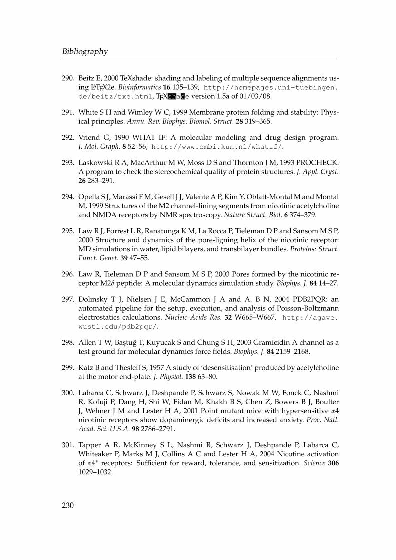
Bibliography
290. Beitz E, 2000 TeXshade: shading and labeling of multiple sequence alignments us-ing LATEX2e. Bioinformatics 16 135–139, http://homepages.uni-tuebingen.de/beitz/txe.html, TEXshade version 1.5a of 01/03/08.
291. White S H and Wimley W C, 1999 Membrane protein folding and stability: Phys-ical principles. Annu. Rev. Biophys. Biomol. Struct. 28 319–365.
292. Vriend G, 1990 WHAT IF: A molecular modeling and drug design program.J. Mol. Graph. 8 52–56, http://www.cmbi.kun.nl/whatif/.
293. Laskowski R A, MacArthur M W, Moss D S and Thornton J M, 1993 PROCHECK:A program to check the stereochemical quality of protein structures. J. Appl. Cryst.26 283–291.
294. Opella S J, Marassi F M, Gesell J J, Valente A P, Kim Y, Oblatt-Montal M and MontalM, 1999 Structures of the M2 channel-lining segments from nicotinic acetylcholineand NMDA receptors by NMR spectroscopy. Nature Struct. Biol. 6 374–379.
295. Law R J, Forrest L R, Ranatunga K M, La Rocca P, Tieleman D P and Sansom M S P,2000 Structure and dynamics of the pore-ligning helix of the nicotinic receptor:MD simulations in water, lipid bilayers, and transbilayer bundles. Proteins: Struct.Funct. Genet. 39 47–55.
296. Law R, Tieleman D P and Sansom M S P, 2003 Pores formed by the nicotinic re-ceptor M2δ peptide: A molecular dynamics simulation study. Biophys. J. 84 14–27.
297. Dolinsky T J, Nielsen J E, McCammon J A and A. B N, 2004 PDB2PQR: anautomated pipeline for the setup, execution, and analysis of Poisson-Boltzmannelectrostatics calculations. Nucleic Acids Res. 32 W665–W667, http://agave.wustl.edu/pdb2pqr/.
298. Allen T W, Bastug T, Kuyucak S and Chung S H, 2003 Gramicidin A channel as atest ground for molecular dynamics force fields. Biophys. J. 84 2159–2168.
299. Katz B and Thesleff S, 1957 A study of ‘desensitisation’ produced by acetylcholineat the motor end-plate. J. Physiol. 138 63–80.
300. Labarca C, Schwarz J, Deshpande P, Schwarz S, Nowak M W, Fonck C, NashmiR, Kofuji P, Dang H, Shi W, Fidan M, Khakh B S, Chen Z, Bowers B J, BoulterJ, Wehner J M and Lester H A, 2001 Point mutant mice with hypersensitive α4nicotinic receptors show dopaminergic deficits and increased anxiety. Proc. Natl.Acad. Sci. U.S.A. 98 2786–2791.
301. Tapper A R, McKinney S L, Nashmi R, Schwarz J, Deshpande P, Labarca C,Whiteaker P, Marks M J, Collins A C and Lester H A, 2004 Nicotine activationof α4∗ receptors: Sufficient for reward, tolerance, and sensitization. Science 3061029–1032.
230

Bibliography
302. Bostick D L and Berkowitz M L, 2004 Exterior site occupancy infers chloride-induced proton gating in a prokaryotic homolog of the ClC chloride channel. Bio-phys. J. 87 1686–1696.
303. Cohen J and Schulten K, 2004 Mechanism of anionic conduction across ClC. Bio-phys. J. 86 836–845.
304. Corry B, O’Mara M and Chung S H, 2004 Conduction mechanisms of chloride ionsin ClC-type channels. Biophys. J. 86 846–860.
305. Faraldo-Gomez J D and Roux B, 2004 Electrostatics of ion stabilization in a ClCchloride channel homologue from Escherichia coli. J. Mol. Biol. 339 981–1000.
306. Miloshevsky G V and Jordan P C, 2004 Anion pathway and potential energy pro-files along curvilinear bacterial ClC Cl− pores: electrostatic effects of chargedresidues. Biophys. J. 86 825–835, http://www.biophysj.org/cgi/content/full/86/2/825.
307. Yin J, Kuang Z, Mahankali U and Beck T L, 2004 Ion transit pathways and gatingin ClC chloride channels. Proteins: Struct. Funct. Genet. 57 414–421.
308. Saparov S M and Pohl P, 2004 Beyond the diffusion limit: Water flow through theempty bacterial potassium channel. Proc. Natl. Acad. Sci. U.S.A. 101 4805–4809.
309. Kim J and Raushel F M, 2004 Access to the carbamate tunnel of carbamoyl phos-phate synthetase. Arch. Biochem. Biophys 425 33–41.
310. Harris R A, 1999 Ethanol actions on multiple ion channels: which are important?Alcoholism Clin. Exp. Res. 23 1563–1570.
311. Davies D L, Trudell J R, Mihic S J, Crawford D K and Alkana R L, 2003 Ethanolpotentiation of glycine receptors expressed in Xenopus oocytes antagonized by in-creased atmospheric pressure. Alcoholism Clin. Exp. Res. 27 743–755.
312. Davies D L, Crawford D K, Trudell J R, Mihica S J and Alkana R L, 2004 Multiplesites of ethanol action in α1 and α2 glycine receptors suggested by sensitivity topressure antagonism. J. Neurochem. 89 1175–1185.
313. “Sullivan, Louis”, Encyclopædia Britannica, http://search.eb.com/eb/article?tocId=9070265, retrieved 2004-10-29 from Encyclopædia BritannicaOnline.
314. Sullivan L H, 1896 The tall office building artistically considered. Lippincott’sMagazine http://www.njit.edu/old/Library/archlib/pub-domain/sullivan-1896-tall-bldg.htm, accessed online 2004-10-29.
315. Baranyai A, 2002 Direct estimation of the partition function from computer simu-lations. Phys. Rev. E 65 026110.
231
Bibliography
316. Weisstein E W, Viviani’s curve, From MathWorld—A Wolfram Web Resource.,http://mathworld.wolfram.com/VivianisCurve.html, accessed 2004-10-19.
317. Wolfram Research, Inc., 2003 Mathematica (Wolfram Research, Inc., Champaign,Illinois), version 5.0.
318. Good R H, 2001 Elliptic integrals, the forgotten functions. Eur. J. Phys. 22 119–126.
319. Free Software Foundation, 1991, GNU General Public License, http://www.gnu.org/copyleft/gpl.html.
320. Grubmuller H, 2003 What happens if the room at the bottom runs out? A closelook at small water pores. Proc. Natl. Acad. Sci. U.S.A. 100 7421–7422.
321. Sansom M S P, Bond P, Beckstein O, Biggin P C, Faraldo-Gomez J, Law R J, Pa-targias G and Tieleman D P, 2002 Water in ion channels and pores—simulationstudies, in Ion channels: from atomic resolution physiology to functional genomics(edited by G Bock and J A Goode), vol. 245 of Novartis Foundation Symposia,66–78, Novartis Foundation, London (John Wiley & Sons, Chicester), http://doi.wiley.com/10.1002/0470868759.ch6.
232

Index
∆G‡, see barrier, as the maximum in thePMF
acetylcholine binding protein, 124, 161AChBP, see acetylcholine binding
proteinage of the universe, 26n, 48nalcohol, 157all-or-none mechanism, 156α7 receptor, 161alpro program, 123ammonia channel, 9AmtB, 9apbs program, viii, 56, 110, 131aquaglyceroporins, see aquaporinaquaporin, 3, 8, 57, 81aromatic belt, 129Arrhenius law, 48natomic force microscopy, 68atomic sphere, 174average, 26
canonical, 20ensemble —, 26grand canonical, 20time —, 26
Avogadro’s constant, 56na ri3Dc program, 31, 63, 195, 197
backbone restraints, 130, 132effect on PMF, 146
balls and springs model, 35barrier
analytic expression, 113as the maximum in the PMF, 108desolvation, 86, 99dielectric, see also Born barrier, 108difficulty of overcoming, 48nfor a Na+ permeating a membrane
mimetic slab, 113
for a Na+ permeating a pore, 113for uncharged NH3, 9in nAChR, 143length of pore, 118local flexibility of wall, 117sensitivity to force field, 146to ion permeation, 102, 108vapour-filled pore, 72
Berendsen coupling, see couplingmethods, weak —
Big Crunch, 26nbits, 123Bjerrum length, 113Boltzmann’s constant, 19bond-stretching potential, 36Born barrier, 8
in α7, 163in model pores, 113in nAChR, 127
Born energy, 108, 109Born profile, 56, 109, 110
α7 receptor, 161, 162model pores, 113nAChR, 135
Born radius, 56, 110nBorn-Oppenheimer approximation, 33boundary, 31, 169
topologically consistent, 170nvariational definition, 170n
Box-Muller method, 206building blocks, 85bulk water, 71bursts, see collective effects
canonical ensemble, 19capillary condensation and
evaporation, 80capillary waves, 70
233
INDEX
capsaicin, 104ncarbamate, 157carbamoyl phosphate synthetase, 9, 157carbon monoxide
dedydrogenase/acetyl-CoAsynthase, 10
carbon nanotube, 80, 82carrier, 2centre of mass removal, 44channel, 2chemical potential, 18chilli peppers, 104nclassically allowed region, 166ClC, 5closed system, 18nClustalW program, 122collective effects, 80, 83, 114combination rules, 36compartmentation, 1condensation, 74conductance
of α7 receptor, 163of nAChR (Torpedo), 150
conductivity, 3constrained free energy, 27, 63n, 64contact angle, 11, 12, 90, 93, 102
and surface tension, see Youngequation
experimental values for water, 93macroscopic, 93microscopic, 93
continuity equation, 66continuum, see solvent, treated as —correlation time
of umbrella sampling steps, seeumbrella sampling
Coulomb interaction, 36, 42force calculation, 44
Coulomb’s law, see Coulombinteraction
coupling methodsextended Hamiltonian, 44weak —, 44, 45
critical radius, 82, 101
crystalline surface, 60current density, 68cylinder-sphere, see sphere-cylinder
Debye length, 56DelPhi program, 56, 129density, 21, 48n
as order parameter, 64from RG, see local densitylocal, see local densityof Cl−
in hydrophobic pores, 99in nAChR, 138
of Na+
in hydrophobic pores, 99in nAChR, 138in wide pores, 114
of waterin hydrophobic pores, 73, 99in nAChR, 137in wide pores, 114near a hydrophobic slab, 74
density of states, 167depletion layer, 71
of ions, 113of water, 69
desensitized state, 148desolvation barrier, see barrier,
desolvationdielectric barrier, see barrier, dielectricdielectric boundary, 165dielectric constant
of implicit solvent, 111of membrane mimetic, 111
dielectric plug, 127diffusion, 70diffusion coefficient, 66, 66–68, 80
at a hydrophobic slab, 71in nAChR, 150
diffusion constant, see diffusioncoefficient
dihedralOPLS-AA potential, 37angle, 37impropers, 37
234

INDEX
potential, 37docking, 165DOS, see density of statesdouble layer, 139δR, see pore, radius correction
effective fluid-wall interaction, 82, 96effective pore radius, 63effective volume, 166Einstein crystal, 60, 60nEinstein relation, 66, 67electrolyte, 101, 115electrostatic barrier, see barrier,
dielectricelectrostatic binding energy, 56electrostatic interaction, see Coulomb
interactionelliptic integrals, 177nensemble average, see averageensemble pore profile, see pore profileentropy, 18enzyme tunnel, 9–10, 157equilibrium flux, see fluxergodic theorem, 26evaporation, 74, 83Ewald summation, 42excess free energy, 18external potential, 20extracellular rings, see also nicotinic
acetylcholine receptor, chargedrings, 124, 128, 136, 144
fakepmf program, 52, 202, 204Fick’s law, 66flexibility, 95, 104
of nAChR pore, 148fluid, 17nflux, 68, 82, 101, 191
analysis algorithm, 192flying ice cube effect, 44force field, 34
AMBER, 131nGROMOS96, 38
nAChR, 145OPLS-AA, 38
nAChR, 132comparison for nAChR, 145effect on PMF, see potential of mean
forceions, 40potential functions, 34protein parameters, 38water, 39
form follows function, 158free energy density, 76free energy difference
between open and closed states, seepore states
maximum from equilibriumtrajectory, 78
temperature dependence, 103–104free energy of solvation, 108free energy profile, 47free particle, 168
gA, see gramicidin Agas channels, 9, 10gaseous state, 17ngate, 3, 4
in nAChR, 60, 124, 126, 128, 137,143
local sidechain block, 5salt-bridge, 5steric occlusion, 5, 124
gating, 3, 4–9physical principles, 86
gating mechanism, 4genpr program, 179Gibbs dividing surface, 28, 165Gibbs free energy, see Gibbs functionGibbs function, 18, 27glutamate synthase, 10glutamine amido transferases, 9gOpenMol program, 197, 199gramicidin A, 81
conductance, 150grand canonical ensemble, 20
for fluid in finite size pore, 63grand potential, 18, 27, 90
for fluid in finite size pore, 63, 63n
235

INDEX
gridfor density calculation, 63in Poisson-Boltzmann calculations,
111gromacs program, 34, 41, 61, 88, 109,
132, 179, 182, 202grompp program, 182, 184, 185Grotthuss mechanism, 8g count program, 62, 188g flux program, 191g ri3Dc program, 63, 189, 195, 197g wham program, 52, 186, 200–202, 204,
205
Hamiltonianof a homogeneous system, 19of a system with a wall, 21
harmonic oscillatorthermally driven, 95
Helmholtz free energy, 18, 27, 63nhole program, 6, 29, 125, 126, 131, 143,
146, 162homogeneous system, 19hydration energy, 113hydration shell, 86, 108, 113, 115hydrophilic groups, 82hydrophobic effect, 1, 10hydrophobic gate, 8, 86, 152hydrophobic gating, 91, 101, 104
— hypothesis, 8hydrophobic girdle, 7, 127hydrophobic residues, 8, 60
conserved in M2, 122hydrophobic slab, 46n, 60, 130hydrophobicity, 11, 81, 82
in docking, 165
implicit solvent, 110information content, 123inhomogeneous system, 20–23interface
ill defined, 28intermediate ring, see also nicotinic
acetylcholine receptor, chargedrings, 124, 128
INTERPRO database, 122intracellular ring, see also nicotinic
acetylcholine receptor, chargedrings, 127
intrinsic chemical potential, 21ninvariance
of scale, see renormalizationinverse temperature, 19ion exclusion layer, 101, 138ion flux, 101ion parameters, 40ion permeation
through low dielectric pores, 108ionic density, 113ionic radius, 6ionic strength, 56
effect on PMF, see potential of meanforce
ionsbarrier to permeation, see barrierin nAChR, 138–141interaction with wall, see wall-ion
interactionpermeation, 101–102
Jalview program, 122just so story, 8
KcsA, 4, 6, 119water conduction, 156
Kelvin equation, 80KirBac1.1, 6Kirkwood-Buff formula, 24
layeringof water, 99
in a hydrophobic pore, 72near a hydrophobic slab, 68
leap-frog integrator, 41Lennard-Jones potential, 35
thermally coarse grained, 97WCA decomposition, see
Weeks-Chandler-Andersondecomposition
life, 1
236
INDEX
ligand gated ion channels, 122, 122and sobriety, 157comparison of M2 region, 123
liquid state, 17nliquid water
in pore, 73phase destabilization, 73phase stabilization, 82
liquid-liquid interface, 70liquid-vapour interface, 94liquid-vapour oscillations, 72, 92
driven by pressure fluctuations, 81in nAChR, 137, 146kinetics, 74
liquid-vapour surface tension, 93local density, 31local flexibility, see pore, local flexibility
of wall
M2 helices, 122, 124, 135alignment, 127in gating, 124
makelogo program, 123Mathematica program, 176mdrun program, 185, 200–202, 205mean square deviation, 68mean square displacement, 67mechanosensitive channels, see also
MscS and MscL, 7membrane
early origin, 1membrane mimetic, see hydrophobic
slabmenthol, 104nmethane, 60methyl groups, 60moat, 143molecular dynamics, 34MscL, 7MscS, 7, 7n, 137, 137n, 145, 156MthK, 4, 6
nAChR, see nicotinic acetylcholinereceptor
neat water, 62
neutron diffraction, 69Newton’s equations of motion, 34nicotine addiction, 150nicotinic acetylcholine receptor, see also
α7 receptor, 5, 7, 102, 124–128alignment of subunits, 127barrier to ion permeation, 143Born profile, 135charged rings, 127, 134, 135t, 138density, 136–141, 145–146ensemble pore profile, 141gate, see gateligand binding domain, 122, 124,
135, 161mutations, 150outer scaffold, 130, 134, 163PMF, 141–144, 146–148pore profile, 126reliability of structure, 130nselectivity filter, see selectivity filtertransmembrane domain, 121, 128,
134, 161transmembrane pore, 125
non-bonded interactions, 35
OmpA, 5open system, 18openness, 65, 72, 89, 91, 92, 94, 99osmotic permeability coefficient, 81
P1 model, 130packing of wall atoms, 83pair correlation function, 22pair distribution function, 22, 23partial trace, see traceparticle mesh Ewald methods, 43
parameters, 44particle reservoir, 89partition function, 19, 20
of a single particle, 169Pauli exclusion principle, 35Pauling radius, see ionic radiusPDB2PQR web service, 131peptide bond, 87periodic boundary conditions, 42, 192
237
INDEX
permeation barrier, 1, 4, 108, 117, 152permeation time, 77, 192Pfam, 122PFAM database, 122pgeom program, 60, 179, 181phase space, 27pKa, 56, 129
pair energy cutoff, 130planar surface, 68PME, see particle mesh Ewald methodsPMF, see potential of mean forcePoincare cycles, 26Poisson equation, 55Poisson-Boltzmann, 110, 131, 135
failure in aqueous pores, 113Poisson-Boltzmann equation, 55pore, 2
amphipathic, 92apolar, see pore, hydrophobicchemical character of wall, 86effective radius, 30effective volume, 30geometry, 86hydrophilic, 87, 93hydrophobic, 60, 87, 92length, 118, 181local flexibility of wall, 86, 95–99,
117polar, see pore, hydrophilicradius, 174, 181, 188radius correction, 30, 189radius from RG, see pore profile,
ensemble —pore model, 60, 60, 87
building of —, 181pore occupancy, 62, 63, 66, 188pore profile, 30
ensemble —, 31pore states, 71
analysis, 89free energy difference, 65, 75, 76,
90, 92thermodynamic model, 90–92
lifetimes, 65, 74
metastable, 76open or closed, 65, 89thermodynamically stable, 76
potential of mean force, 46, 108and ionic strength, 146and water model, 146combining equilibrium and
umbrella sampled profiles, 110errors, 143from equilibrium density, 48, 63,
109from umbrella sampling, 109of Cl−
in nAChR, 142, 143, 147of Na+
in α7, 162in hydrophobic pores, 113in nAChR, 142, 143, 147
of waterand flexibility, 117and pore length, 118in hydrophobic pores, 114in nAChR, 141, 142, 147
probability distribution, 205sensitivity to force field, 146
power law, see invariance, of scaleprepconflist.pl program, 185–187prepumbrella.pl program, 182, 184–186pressure, 18
coupling, 45parameters, 46
in simulations, 45procheck program, 130protonation states, 129, 134pulsed water transport, 83
quantum mechanics, 32, 35
radial distribution function, 22, 115radius
and wall roughness, 188nfrom shifted van der Waals surface,
29radius of gyration, 30n
of a fluid, 30, 198
238
INDEX
Raster3D program, 6, 88, 108, 162rate theory, 102reaction coordinate, 47rejection method, 206renormalization, see power lawresidency time, 189resting state, 148RG, see radius of gyrationRMSD, see root mean square deviationroot mean square deviation, 26
and local flexibility, 95bound particle, 26diffusing particle, 27of membrane mimetic, 68of wall atoms, 95
Ryckaert-Bellemans potential, 37
scaffold, see nicotinic acetylcholinereceptor, outer scaffold
Schrodinger equation, 33selectivity, 3selectivity filter, 6n, 86, 119
in K channels, 126in nAChR, 126, 144, 151
self-diffusion coefficient, see diffusioncoefficient
sensor, 3sequence logo, 122, 123Shannon entropy, 123shape function, 169simplified pore model, 87solid state, 17nsolute cavity, 108solvation free energy, 86solvent
treated as continuumin electrostatics, 55, 114in thermodynamics, 94
treated explicitlyin molecular dynamics, 39
solvent cavity, 75spatial oscillations, see layeringSPC, see water modelsphere-cylinder
cut-out volume, 177
interface, 174intersection, 174–178
SPME, see particle mesh Ewaldmethods
squidginess, 28Sullivan, Louis, 158surface, 115, 165
Gibbs —, see Gibbs dividingsurface
hydrophobic, 93ill defined, 28methyl terminated, 93MSMS, 178re-entrant, 29, 29n, 173solvent accessible, 31, 32nsolvent excluded, 32n, 32, 108, 173van der Waals, 29n, 29
surface force apparatus, 68surface free energy, see surface tensionsurface tension, 11, 18, 17–19, 81, 90,
102and contact angle, see Young
equationand flexibility of wall, 99
survival probability, 74
temperature, 18coupling, 45
parameters, 45in simulations, 44
temperature-sensitive channels, seeTRP channels
thermal broadening, 97thermal vibrations, 26thermodynamic average, 20time average, see averagetime series, 65, 74TIP4P, see water modeltotal energy, 18toy model, 13Tr, see tracetrace, 19
partial, 27trajectory, 34transition point, 76
239

INDEX
transition radius, see critical radiustransition state, 66transport
active, see carrierpassive, see channel or pore
TRP channels, 104tryptophan synthase, 9two point density correlation function,
22
umbrella potential, 49umbrella sampling, 49
confinement potential, 202correlation time of sampling steps,
110drift correction, 53equilibration, 53equilibration time, 110in nAChR, 133matching profiles, 53probability distribution, 205simulated, 204symmetrization of profiles, 110
uniform deviate, 206Ursell function, 22
vapourvs. gas, 10n
vapour-lock, 137n, 156Verlet integrator, 40Viviani’s curve, 173vmd program, 6, 88, 108, 125, 131, 141,
162, 197volume, 18, 165
at molecular scale, 28effective, see effective volumefrom shifted van der Waals surface,
29ill defined, 28rugged, 173
wallas an external field, 20, 97, 166flexibility, see pore, local flexibility
of wall
thermal broadening, seeLennard-Jones potential,thermally coarse grained
wall-ion interaction, 115wall-water interaction, 82water
as permeant species, 57as solvent, 57dynamical properties in pores, 77in confinement, 58in nAChR, 136–138in pores, 91interaction with wall, see
wall-water interactionliquid, see liquid water
water channels, 8water flux, 101water layer, 69, 73, 95, 114water model
effect on PMF, see potential of meanforce
SPC, 39, 39tTIP4P, 39, 39t
water radius, 6water vapour
bubble, 74in pore, 73, 89
WCA, see Weeks-Chandler-Andersondecomposition
WEBLOGO web service, 123Weeks-Chandler-Anderson
decomposition, 32n, 97thermal broadening, 97
Weighted Histogram Analysis Method,see WHAM, 110
WHAM, 50, 133, 200drift correction, 54tests of, 52, 204tolerance, 110
WHAM equations, 51WhatIf program, 129–131window potential, see umbrella
potential
xfarbe program, 72, 116, 180, 197
240

INDEX
xmgrace program, 202
Young equation, 11, 80, 91
Zustandssumme, see partition function
241