principles of ece theory part ii - dr. myron … · principles of ece theory part ii ... lindstrom,...
TRANSCRIPT
PRINCIPLESOF
ECE THEORYPART II
A NEW PARADIGM OF PHYSICS
Myron W. Evans, Horst Eckardt, Douglas W. Lindstrom,Stephen J. Crothers, Ulrich E. Bruchholz
Edited and collated by Horst Eckardt
May 9, 2017

Texts and figures: c© by Myron W. Evans, Horst Eckardt,Douglas W. Lindstrom, Stephen J. CrothersCover design: c© by Manfred FeigerTypesetting: Jakob Jungmaier
ISBN X-X-X-X
Published by the authors, 2017, all rights reserved
Print: epubli, a service of neopubli GmbH, Berlin, Germany
2

This book is dedicated toall wholehearted scholars of natural philosophy
i

ii

Preface
xxxxxxxx xxxxxxx xxxxxxx xxxxxxxx xxxxxxxx xxxxxxxx xxxxxxx xxxxxxxxxxxxxxx xxxxxxxx xxxxxxxx xxxxxxx xxxxxxx xxxxxxxx xxxxxxxx xxxxxxxxxxxxxxx xxxxxxx xxxxxxxx xxxxxxxx xxxxxxxx xxxxxxx xxxxxxx xxxxxxxxxxxxxxxx
Craig Cefn Parc, 2017 Myron W. Evans
iii

PREFACE
iv

Contents
1 Introduction 3
2 The Effect of Torsion on Geometry 13
3 The Field Equations of ECE 2 21
4 Orbital Theory 47
5 New Spectroscopies 79
6 The ECE 2 Vacuum 109
7 Precessional Theory 125
8 Triple Unification: Fluid Electrodynamics 151
9 Triple Unification: Fluid Gravitation 179
10 Stephen Crothers 201
11 Unified Field Theory of the Rainich Space: Determining Prop-erties of Elementary Particles 20311.1 Introduction . . . . . . . . . . . . . . . . . . . . . . . . . . . . . 20311.2 The Equations . . . . . . . . . . . . . . . . . . . . . . . . . . . 20411.3 Explanation of the Numerical Method . . . . . . . . . . . . . . 20511.4 Determination of the Parameters . . . . . . . . . . . . . . . . . 20611.5 The Singularity Problem and its Solution . . . . . . . . . . . . 20611.6 Numerical Simulations . . . . . . . . . . . . . . . . . . . . . . . 20711.7 Computational Results . . . . . . . . . . . . . . . . . . . . . . . 21011.8 Conclusion . . . . . . . . . . . . . . . . . . . . . . . . . . . . . 212
1

CONTENTS
2

Chapter 1
Introduction
The first volume of this book [1] (see also [2] - [24]), is entitled “Principles ofECE Theory: A New Paradigm Shift of Physics”, (PECE), a paradigm shiftbased on geometry. “Ubi materia ibi geometria”, “where there is matter thereis geometry” was a saying coined by Johannes Kepler several hundred yearsago. The teaching of ECE on www.aias.us and www.upitec.org has madea tremendous impact on physics and the great paradigm shift has developedrapidly. PECE covered the development up to early 2014. Since then a hun-dred further papers have appeared so it is timely and important to review themajor advances contained in them, beginning with UFT 313. This paper devel-oped the rigorous second Bianchi identity using the Jacobi and Ricci identities.This was the method used by Bianchi and earlier by Ricci, However, spacetimetorsion was unknown in their time so they proceeded with a curvature basedtheory. UFT 313 rigorously corrects their work for the presence of torsion, firstinferred by Cartan and others in the early twenties. By basing the correctionin the fundamental Jacobi identity, a rigorous new identity emerges, namedthe Jacobi Cartan Evans (JCE) identity purely in order to distinguish it fromother identities in the literature.
The first and by now famous development of the second Bianchi identityin UFT 88 has made its way around the best universities in the world becauseit is the first paper to realize that the structure of the Einsteinian general rel-ativity is changed completely and fundamentally by torsion. The ECE theoryis based on torsion, and from the outset re-established the correct geometry.UFT 88 was followed by UFT 99, which uses the commutator method to showthat if torsion is zero then curvature is zero. So neglect of torsion means thatthe Einstein theory is fundamentally erroneous. The Einsteinian curvature iszero, so its gravitational field is zero, reductio ad absurdum. About a dozendefinitive proofs were spun off from UFT 99 and all have been read avidly fornearly a decade, without any objection. Nothing could be a clearer demonstra-tion of the complete failure of the Einstein theory. It was an influential theoryin its time, but progress means that it is now obsolete. The UFT papers nowshow many faults in the Einstein theory, which is greatly improved by ECE 2.
It was decided to base ECE 2 on the JCE identity because it in turn is
3

based on the rigorous Jacobi identity. This required the use of the Evans tor-sion identity of UFT 109, and of the Ricci identity generalized for torsion. Thetensor algebra of UFT 313 must be translated to vector algebra in order todefine the geometry of the ECE 2 field equations. These are field equations ofgravitation, electrodynamics, fluid dynamics and indeed any area of physics,a demonstration of the fundamental meaning of a generally covariant unifiedfield theory. This translation was carried out in UFT 314 and forms part ofchapter two on geometry. Chapter two is a synopsis of UFT 313, UFT 314and UFT 354. The latter shows that correct consideration of torsion in thefundamental theorem of metric compatibility completely changes the relationbetween connection and metric used by Ricci, Bianchi, and later Einstein.UFT 354 concludes that the torsion tensor must be completely antisymmetric,in all three indices, a new discovery in fundamental geometry that goes be-yond Cartan’s work. This means that Einstein’s field equation is completelyincorrect. The field equation of Einstein was abandoned after the realizationsand implications of UFT 88 were accepted worldwide.
The ECE 2 vector geometry of UFT 314 produces a structure which is su-perficially similar to the electromagnetic field equations of special relativity,which are Lorentz covariant in a Minkowski spacetime as is well known. InMinkowski spacetime however, both torsion and curvature are zero. The ECE 2field equations are generally covariant in a mathematical space in which bothtorsion and curvature must be non zero. This is a fundamental requirementof any geometry in any mathematical space of any dimension. As shown inUFT 99, the requirement follows from the action of the commutator of covari-ant derivatives on any tensor, for example a vector. The result of the operationof the commutator on the vector is to define the curvature and torsion simul-taneously. This is demonstrated in full detail in UFT 99 and in the definitiveproofs. The latter are simplifications of UFT 99. The obsolete physics removedthe torsion tensor arbitrarily by use of a symmetric connection and continuedto neglect torsion incorrectly. The symmetric connection implies a symmetriccommutator, which vanishes, so the curvature vanishes if torsion is arbitrarilyneglected. ECE does not use an arbitrary “censorship” of torsion.
UFT 315 introduced a new fundamental axiom, which showed that thefield equations could be based on curvature as well as torsion. This realizationgreatly extends the scope of the original ECE field equations. The curvaturebased equations were based on the JCE identity. This new axiom is the basisof ECE 2 and is developed in chapter three, on electrodynamics and gravita-tion, and following chapters. The field equations were simplified by removalof internal Cartan indices so their mathematical structure is also simplified.It looks identical to the Maxwell Heaviside (MH) field equations but with bigdifferences and advantages. The key difference is that the field equations ofECE 2 are generally covariant in a space with non zero torsion and curvature.The general covariance of ECE 2 reduces to Lorentz covariance, but the under-lying mathematical space is one in which the torsion and curvature are bothzero. This was given the name “ECE 2 covariance”.
The ECE 2 field equations of electrodynamics, gravitation, fluid dynamics,and any subject area of physics are all Lorentz covariant in a space with
4

CHAPTER 1. INTRODUCTION
finite torsion and curvature. The property of Lorentz covariance has the greatadvantage of allowing the use of properties which up to the emergence of ECE 2were associated with special relativity in Minkowski spacetime. For examplethe hamiltonian and lagrangian, and the Lorentz force equation. However,ECE 2 has a considerably richer structure than special relativity, and ECE 2has the overwhelming advantage of being able to unify what are thought tobe the fundamental force fields of nature: gravitation, electromagnetism, weakand strong nuclear fields. Unification takes place with ECE 2 covariance.
ECE 2 offers a much greater flexibility in the definitions of fields and po-tentials than ECE, so there is considerable scope for development. Chapterthree of this book exemplifies this development with UFT 315 to UFT 319,which define the ECE 2 field equations of gravitation and electromagnetismand draw several completely original inferences. In UFT 316 the earlier, tor-sion based, axioms of ECE theory were augmented by curvature based axioms,and this is the key advance given the appellation ECE 2 theory. For examplethe magnetic flux density can be defined in ECE 2 as being proportional tospin torsion and also as being proportional to spin curvature. In the first casethe proportionality is the scalar magnitude of vector potential, in the secondcase it has the units of magnetic flux, which is weber. Similarly the electricfield strength is defined in ECE 2 as being proportional to the orbital torsion,and also as being proportional to the orbital curvature. Another key insightof UFT 316 is that internal Cartan indices can be removed, resulting in fieldequations that look identical to the Maxwell Heaviside equations (MH), butthese are field equations defined in a space with finite torsion and curvature.This is the essence of ECE 2 theory.
In UFT 317 the complete set of equations of ECE 2 electrodynamics is givenwithout internal Cartan indices. In general the magnetic charge current den-sity is non zero, and vanishes if and only if a choice of spin connection is made.The set of equations is based directly on Cartan geometry and has the sameformat as the MH equations in a mathematical space with non zero torsionand curvature. This poperty defines ECE 2 covariance and also defines specialrelativity in a space with non zero torsion and curvature. In ECE 2, bothtorsion and curvature are always non zero as required by fundamental consid-erations of the commutator described already. This is true of any geometry inany dimension in any mathematical space. The space of ECE 2 is four dimen-sional - spacetime. The spin connection enters directly in to these equations.In UFT 317 the continuity equation of ECE 2 is derived from geometry and anew set of field potential relations is defined.
In UFT 318 the ECE 2 field equations of gravitation are derived from thesame Cartan geometry as the field equations of electromagnetism, so a gener-ally covariant unified field theory is derived. The gravitational field equationsare also ECE 2 covariant, and have the same overall properties as electromag-netism. Example properties are given in UFT 318: antisymmetry, equivalenceprinciple, counter gravitation and Aharonov Bohm effects. Newtonian gravi-tation is a small part of ECE 2 gravitational field theory.
This fact is emphasized in UFT 319, which develops Newtonian and nonNewtonian gravitation. The Newtonian limit of ECE 2 gravitational theory
5
is defined, and the ECE 2 antisymmetry law used to derive the equivalenceprinciple between gravitational and inertial mass. Non Newtonian effects inECE 2 are exemplified by light deflection due to gravitation, simple estimates ofphoton mass are made. These major advances have made UFT 319 a popularpaper, currently being read about one thousand two hundred times a yearfrom combined sites www.aias.us and www.upitec.org. The combined ECE 2papers used as the basis of this book are currently being read about forty onethousand times a year.
The advances made in UFT 313 to UFT 319 form the basis for chapters twoand three of this book. Chapters Five and Six develop the ECE 2 covarianceprinciple from relevant source papers. In UFT 320 the gravitomagnetic Lorentztransform is developed on the basis of ECE 2 covariance, which is defined asLorentz covariance in a space with finite torsion and curvature. Applying theECE 2 transform to the field tensor of gravitation produces the Lorentz forceequation, which is in general relativistic. The gravitomagnetic Biot Savart andAmpere laws are developed for comparison. The laws are applied to planarorbits to find the gravitomagnetic field of the orbit and the current of massdensity of the planar orbit. The method is generally valid and can be used onall scales.
In UFT 322, perihelion precession and light deflection due to gravitationare developed with the gravitomagnetic Ampere law of ECE 2. The ECE 2gravitomagnetic field is developed for dynamics in general and for an orbitin three dimensions. For two dimensional orbits the perihelion precession andlight deflection due to gravitation are expressed in terms of the gravitomagneticfield of the relevant mass. In UFT 323 orbital theory in general is developed interms of the Lorentz transform of the field tensor of ECE 2 gravitomagnetic anddynamic theories. The concept of Lorentz transform is extended to the Lorentztransform of frames. In ECE 2 the Lorentz transform becomes a concept ofgeneral rather than special relativity. The theory is applied to an a prioricalculation of the perihelion precession in terms of the gravitomagnetic field.
In UFT 324 the relativistic Binet equation (RBE) is inferred and used tosolve the Lorntz force equation of ECE 2. The RBE is inferred from theSommerfeld hamiltonian and relativistic orbital velocity calculated straight-forwardly. The orbital velocity equation is used to derive the velocity curveof a whirlpool galaxy and also to give a precise explanation of the deflectionof light and electromagnetic radiation due to gravity. These major advancesare collected in Chapter Seven and overthrow the obsolete Einstein theory. InUFT 325 the solution of the ECE gravitomagnetic Lorentz force equation isexpressed in terms of the ECE 2 covariant hamiltonian and lagrangian. Thelagrangian is the classical Sommerfeld lagrangian and is solved by computer al-gebra and relativistic methods. A scatter plot method is used to infer the trueprecessing orbit. It is shown that this is not the result of the Einstein theory,which develops severe difficulties. Therefore ECE 2 gives the exactly correctresult both for perihelion precession and light deflection due to gravitation.
Chapter Five deals with quantization of ECE 2 and applications to spec-troscopy. Several new types of spectroscopy are inferred. Quantization isbased on ECE 2 covariance, so the quantization of special relativity can be
6

CHAPTER 1. INTRODUCTION
applied but in a space with finite torsion and curvature. Various schemes ofquantization are developed in UFT 327, resulting in new types of shifts thatcan be tested experimentally. A new axiom of ECE 2 relativity is introduced,that the laboratory frame velocity of the ECE transform is bounded above byc/√
2, where c is the universal constant of standards laboratories known asthe vacuum speed of light. This axiom allows a particle of mass m (notablythe photon) to move at c, thus removing many obscurities of standard specialrelativity. The axiom results immediately in the experimentally observed lightdeflection due to gravitation, the “twice Newton” result.
In UFT 327 the ECE 2 metric is used to produce an orbital equation whichcan be interpreted as a precessing ellipse. This result confirms the demon-stration that the lagrangian and hamiltonian of ECE 2 relativity produce aprecessing ellipse without any further assumption. None of the assumptionsused in the obsolete Einstein theory are needed. This is a healthy developmentbecause the Einstein theory is riddled with errors, being fundamentally incor-rect due to neglect of torsion. UFT 327 provides an important demonstrationof the failings of the Einstein theory. Its claims to produce a precessing ellipsefail qualitatively (i.e. completely) due to poor methods of approximation.
In UFT 328 the existence of precessing orbits from ECE 2 relativity is con-firmed using both numerical and theoretical methods. These are used to findthe true precessing orbit using ECE 2 covariance. The true orbit is given by si-multaneous solution of the ECE 2 lagrangian and hamiltonian using numericalmethods. The only concepts used are the infinitesimal line element, lagrangianand hamiltonian of ECE 2 relativity. The analytical problem is in general in-tractable, but the numerical solution is precise. The elaborate and incorrectmethods of Einsteinian relativity are clearly obsolete.
In UFT 329 new types of electron spin resonance (ESR) and nuclear mag-netic resonance (NMR) spectroscopy are developed. These are of general util-ity in atoms and molecules, and in all materials. The novel resonance terms areexpressed in terms of the W potential of ECE 2, which has the same units asthe A potential of the obsolete Maxwell Heaviside (MH) theory. UFT 330 de-velops hyperfine spin orbit coupling theory by replacing the restrictive Diracapproximation. This method reveals the presence of several novel spectro-scopies of great potential utility. New schemes of quantization are proposedand order of magnitude estimates made of the hyperfine splitting.
UFT 331 develops a new type of relativistic Zeeman splitting by discard-ing the Dirac approximation. The Zeeman effect develops an intricate newstructure, which is illustrated graphically and illustrated with the 2p to 3d(visible) transitions, and 4p to 5d (infra red) transitions. The former splitsinto nine lines, the latter into forty five lines. These can be resolved to pro-duce an entirely new spectroscopy. This is a popular paper, heavily studied.It challenges the traditional approach in many ways. UFT 332 follows with theECE 2 theory of the anomalous Zeeman effect, producing novel spectroscopicstructure that can be tested experimentally. This paper shows that the ninetyyear old Dirac approximation implies that the classical hamiltonian vanishes.This unphysical result means that a lot of hyperfine structure has been missed.If this structure exists, it is of great use in the laboratory, if it does not exist
7

there is a crisis in relativistic quantum mechanics. It is become clear thatDirac carefully chose approximations in a subjective manner in order to givethe experimental results. Einstein also used this subjective approach in anincorrect manner.
UFT 333 develops new and rigorous schemes of quantization of ECE 2 rel-ativity. Each scheme leads to different spectral results. The method usedby Dirac in the twenties used a subjective choice of approximation, which istaken literally means that the classical hamiltonian always vanishes, an absurdresult. Dirac avoided the problem by subjective laundering of the approxima-tions. UFT 333 reveals the fragility of this method because it shows thatdifferent rigorous schemes of approximation give different spectra. This meansthat relativistic quantum mechanics is not rigorous, it is a transitional theoryto an as yet unknown theory. Einstein regarded quantum mechanics in muchthe same way, and rejected the Copenhagen interpretation out of hand, withde Broglie, Schroedinger and others.
UFT 334 develops a rigorous test of relativistic quantum mechanics withESR. Two example set ups are used: an electron beam and the anomalousZeeman effect in atoms and molecules. UFT 335 follows up by considering theeffect on NMR of discarding the Dirac approximation, and replacing it withrigorous ECE 2 quantization. There are measurable effects on the chemicalshift, spin orbit and spin spin interaction.
UFT 336 begins a new phase of development of vacuum ECE 2 theory byconsidering the ECE 2 vacuum needed for the Aharonov Bohm (AB) effect.This vacuum is traditionally defined as regions where potentials are non zerobut in which fields are zero. It is shown that the AB vacuum contains anECE 2 vector potential which can cause ESR and NMR in the absence ofa magnetic field. It should be possible to test these effects experimentallyby using a variation of the Chambers experiments. UFT 337 follows up byshowing that the ECE 2 theory is richly structured AB type vacuum and canbe defined entirely by the spin connection. The ECE 2 vacuum can be used toexplain the radiative corrections, so the theory can be tested experimentally.The minimal prescription is defined by the W potential of the ECE 2 vacuum,which is developed in terms of a Tesla vacuum and a relativistic particle flux.
UFT 338 introduces the ECE 2 vacuum particle and defines its mass by us-ing experimental data on the anomalous g factor of the electron. The vacuumparticle mass can be used to define the g factor to any precision. The severelimitations of the Dirac theory of the electron are discussed. These limita-tions are due to the fact that the Dirac approximation, applied directly andliterally, means that the classical hamiltonian always vanishes. The theory ofUFT 338 replaces quantum electrodynamics, which is riddled with subjectivityand which cannot be tested experimentally without the arbitrary adjustmentof variables and the arbitrary removal of infinities known as renormalization.
UFT 339 follows up by developing the dynamics of the ECE 2 vacuum par-ticle. The relativistic hamiltonian of the ECE 2 vacuum is inferred, and theHilbert constant is reinterpreted as the velocity of the vacuum particle multi-plied by the universal power absorption coefficient of UFT 49 on www.aias.us.It is argued that the universe is an equilibrium between elementary and vac-
8

CHAPTER 1. INTRODUCTION
uum particles. This process has no beginning and no end. The mass of theuniverse is made up of the combined mas of elementary and vacuum particlesand there is no “missing mass” as in the obsolete physics. Some examples aregiven of Compton type scattering processes which could be used for experi-mental testing. UFT 340 follows up by developing the ECE 2 theory of theLamb shift from the ECE 2 vacuum, an AB vacuum made up of wave-particleswhich can transfer energy and momentum to elementary particles. A surveyon the vacuum papers is given in chapter Six.
UFT 341 is a paper that deals with gravitational amplification by stimu-lated emission of radiation (GASER). This apparatus design is based on thatof the LASER, and stems from the ECE 2 gravitational field equations, whosestructure is the same as the ECE electromagnetic field equations. The gravi-tational Rayleigh Jeans and Stefan Boltzmann laws are inferred. The energydensity of gravitational radiation, if observed without controversy, is propor-tional to the fourth power of temperature. It is reasonable to assume thatgravitons are absorbed and emitted by atoms and molecules. It may becomepossible to amplify gravitational radiation to the point where it becomes ob-servable in the laboratory.
UFT 342 begins a series of papers on cosmology and develops an exactand simple description of light deflection due to gravitation and perihelionprecession from ECE 2 relativity. Therefore ECE 2 unifies the now obsoletespecial and general relativity. UFT 343 develops Thomas and de Sitter pre-cession from the concepts introduced in UFT 342 and using the foundationaldefinition of relativistic momentum. UFT 344 develops the theory of planetaryprecession as a Larmor precession produced by the torque between the ECE 2gravitomagnetic field of the sun and the gravitomagnetic dipole moment of theEarth or any planet. In general, any observable precession can be explainedwith the ECE 2 field equations. UFT 345 follows up by applying the methodgeodetic and Lense Thirring precessions using ECE 2 gravitomagnetostatics inan ECE 2 covariant theory. The Lense Thirring calculation is in exact agree-ment with Gravity Probe B and the geodetic precessional calculation in goodagreement. UFT 346 is a heavily studied paper and gives a general theory ofany precession in terms of the vorticity. The result is given in terms of thetetrad and spin connection of Cartan geometry. The theory is applied to theplanetary, geodetic and Lense Thirring precessions, giving an exact agreementin each case in terms of the vorticity of the mathematical space of the ECE 2field equations.
In UFT 347 the precession of an elliptical orbit is considered in terms ofthe ECE 2 Lorentz force equation. The method is to use ECE 2 relativityand the minimal prescription. The hamiltonian is defined of a particle in thepresence of a gravitomagnetic vector potential with the units of velocity. Thelagrangian is calculated from the hamiltonian using the canonical momentumand the Euler Lagrange equation used to derive the Lorentz force equation. Inthe absence of gravitomagnetism this equation reduces to the Newton equation.Any precessional frequency of any kind can be described by the precession ofthe Lorentz force equation. UFT 348 follows up by considering the minimalprescription introduced in UFT 347 in order to show that precession emerges
9

directly from the relevant hamiltonian. This is the simplest way to describeprecession. The Leibnitz force equation is augmented by terms which includethe observed precession frequency, and becomes a Lorentz force equation. Fora uniform gravitomagnetic field the force equation can be derived from a simplelagrangian, and the former can be expressed as a Binet equation. UFT 348 isa heavily studied paper.
UFT 349 begins the development of the ECE 2 theory of fluid dynamics andshows that they have the same ECE 2 covariant structure as the ECE 2 equa-tions of gravitation and electromagnetism, thus achieving triple unification interms of ECE 2 relativity described in Chapter Eight. The series UFT 349to UFT 360 is very heavily studied. UFT 349 shows that spacetime turbu-lence can be detected by its effect on a circuit such as that in UFT 311 onwww.aias.us. It is shown that Ohm’s Law and the Lorentz force equation areintrinsic to the ECE 2 field equations, and emerge from their geometry. Theytherefore have equivalents in gravitation and fluid dynamics.
UFT 350 is a posting of “Principles of ECE Theory”. UFT 351 developsthe new subject of fluid electrodynamics. The Reynolds number is incorpo-rated into the calculations, producing the transition to turbulence. Electricpower form spacetime is a direct consequence of fluid electrodynamics. It isshown that the Stokes and convective derivatives are examples of the Cartancovariant derivative. The spin connection for the convective derivative is theJacobian and is a fundamental concept of fluid dynamics and fluid electro-dynamics. Numerical solutions illustrate flows. UFT 352 develops a schemeof computation and animation to calculate the electric field strength (E) andmagnetic flux density (B) imparted to a circuit from the vacuum, or spacetime.All relevant quantities are calculated from the velocity field, which becomesturbulent at a given Reynolds number. It is a heavily studied paper.
UFT 353 generalizes ECE 2 fluid dynamics by introducing viscous effectsusing the most general format of the Navier Stokes and vorticity equations.The resulting structure is that of ECE 2 relativity, and it is shown that thewhole of fluid dynamics can be reduced ot one wave equation. UFT 354 ison connections of the anti symmetric and totally antisymmetric torsion tensorand is incorporated in Chapter Two on fundamental geometry.
UFT 355 is the most heavily studied paper of the ECE 2 series at presentand introduces simple field and wave equations of fluid electrodynamics. Thesedescribe the transfer of energy and power from a fluid spacetime, aether orvacuum to a circuit, notably that of UFT 311. It is shown that the processconserves total energy/momentum and total charge/current density, which aretransferred from fluid spacetime to the circuit. It is followed up by UFT 356,another very heavily studied paper that considers the induction of spacetimeproperties by material fields and potentials. It shows that spacetime is arichly structured fluid described by fluid electrodynamics. The spacetime inturn induces properties in a circuit. UFT 357 verifies fluid electrodynamicsexperimentally by using the well known radiative corrections, known to highprecision experimentally. These include the g factors of elementary particlessuch as the electron, and the Lamb shift in atomic hydrogen. The anomalousg of the electron is explained to any precision with spacetime vorticity and the
10

CHAPTER 1. INTRODUCTION
Lamb shift to any precision with the spacetime potential. All this is subjectof chapter Eight.
UFT 358 introduces the subject area of fluid gravitation, which is ECE 2unification of gravitation with fluid dynamics. In fluid dynamics, the acceler-ation due to gravity, mass density and other fundamental concepts originatein spacetime considered as a fluid. Ultimately, all concepts are derived from amoving frame of reference. It is shown that the main features of a whirlpoolgalaxy can be described with fluid dynamics without the use of dark matter orblack holes. UFT 359 describes spacetime structure generated by Newtoniangravitation, which is illustrated with the velocity field, vorticity, the chargedefined by the divergence of the velocity field, the vorticity (the curl of thevelocity field, the current and so on). These are illustrated with Gnuplotgraphics. This is followed up by UFT 360 which gives the generally covariantinverse square law of all orbits, in which the acceleration due to gravity isdefined as the Lagrange or convective derivative of the orbital velocity. Thisis the derivative in a moving frame of reference and is an example of the co-variant derivative of Cartan. These results on unification of gravitation withfluid dynamics are presented in chapter Nine.
Chapter Ten reviews the invalidity of Kirchhoff’s Law of thermal emis-sion and the non-universality thereby of Planck’s equation for thermal spec-tra, and the implications for the ’CMB’ and Big Bang cosmology. ChapterEleven presents an alternative method of unifying Riemann geometry withelectromagnetism. As a stunning result, properties of elementary particles areobtained. Standard modellers haven even given up to try this.
11

12

Chapter 2
The Effect of Torsion onGeometry
The effect of torsion on Riemannian geometry is profound and far reaching.This was not fully realized until 2003, when the Einstein Cartan Evans (ECE)unified field theory was inferred. It gradually became clear as the ECE series ofpapers progressed that the entire edifice of the Riemennian geometry collapsesif torsion is forced to vanish through use of a symmetric Christoffel symbol.This means that Einsteinian general relativity becomes meaningless, becausethe Einstein field equation is based on torsionless Riemannian geometry. Mostof the obsolete textbooks of the twentieth century do not even mention torsion,and if they do it is regarded as a removable nuisance. These textbooks arebased on the arbitrary and unprovable assertion that torsion does not existbecause the Christoffel connection is by definition symmetric in its lower twoindices.
This meaningless dogma is based on an astonishing inflexibility of thought.A casual glance at the mathematics of the connection shows that it is in generalasymmetric in its lower two indices. It consists of a symmetric part and anantisymmetric part. The latter defines the torsion tensor or its equivalentin Cartan’s differential geometry, the torsion form, a vector valued two formantisymmetric in its lower two indices. The torsion form is defined by oneof the Maurer Cartan structure equations, and the curvature form by theother structure equation. The torsion form is the covariant derivative of thetetrad, and the curvature form is the covariant derivative of the Cartan spinconnection. The torsion and curvature are related by the Cartan identity[2]- [13], and by the Evans identity, inferred in the early UFT papers. TheEvans identity is the Cartan identity for Hodge duals. The Cartan and Evansidentities are the geometrical basis of the field equations of ECE. This is aparadigm shift which led to the first successful unified theory of physics. Ithas been described by Alwyn van der Merwe as the post Einsteinian paradigmshift, and has made an enormous impact on physics, measured accurately bythe scientometrics of www.aias.us.
The second major paradigm shift occurred in UFT 313 onwards on www.
13

aias.us and www.upitec.org. It simplified the ECE equations and intro-duced equations based both on torsion and curvature. The ECE 2 field equa-tions of electrodynamics look like the obsolete Maxwell Heaviside (MH) fieldequations but are written in a mathematical space in which both torsion andcurvature are non zero. This is summarized in chapter one. The secondparadigm shift is called the ECE 2 theory, which has advantages of simplicityand greater scope. The obsolete Einstein field equation is replaced by a setof field equations in ECE 2 theory which look like the MH field equations ofelectrodynamics, but which are written in a space with finite torsion and cur-vature. The MH theory is written in the Minkowski spacetime, which has notorsion and no curvature and which is therefore known as the mathematicalspace of special relativity, which is Lorentz covariant but not generally covari-ant. In the most recent advances of ECE 2, made in the latter half of 2016,the equations of fluid dynamics have also been developed as field equationswhich look like the MH equations, but which are again written in a space withfinite torsion and curvature. So a triple unification has been achieved; thatof gravitation, electrodynamics and fluid dynamics, allowing the possibility ofmajor advances.
The groundwork for the second paradigm shift was laid down in the classicUFT 88, which has been read several tens of thousands of times since it wasinferred in 2007. It has been read in several hundred of the world’s best uni-versities and is an accepted classic. The quality of universities can be rankedby webometrics, Times, Shanghai and QS world rankings for example. Thereadership of ECE and ECE 2 has always been in the world’s best universities,often in the world’s top twenty. UFT 88 was the first attempt to incorporatetorsion into the second Bianchi identity, upon which the Einstein field equa-tion is based directly. UFT 88 shows that the incorporation of torsion changesthe identity completely, so the Einstein field equation was discarded as beingincorrect and obsolete in 2007. The scientometrics of www.aias.us (its fil-tered statistics section and UFT 307 for example), show that the Einstein fieldequation has been discarded completely by a large percentage of the colleaguesinternationally. This is in itself an important paradigm shift of the history ofscience, because a major theory of physics has been discarded by means of theknowledge revolution brought about by the world wide net. Knowledge is nolonger confined within Plato’s dogmatic cave, and once it is out in the open,a freedom to think follows and the light of reason prevails.
In UFT 99 it was shown that the well known commutator method of si-multaneously generating the curvature and torsion tensors also proves that iftorsion vanishes, curvature vanishes. So the arbitrary removal of torsion bythe obsolete physics also removed curvature, leaving no geometry, reductio adabsurdum, Any valid geometry must be developed in a space where torsionand curvature are both identically non-zero. UFT 99 was supplemented by wellknown definitive proofs, which simplified UFT 99 to its essence: the commuta-tor is antisymmetric by definition. The indices of the commutator of covariantderivative are the indices of torsion, so if torsion is forcibly removed by usingequal indices, the commutator vanishes. In consequence the curvature alsovanishes. Removing torsion removes curvature. If curvature is removed the
14

CHAPTER 2. THE EFFECT OF TORSION ON GEOMETRY
entire Einsteinian theory collapses.In UFT 109 a new identity of the torsion tensor was inferred and was named
the Evans torsion identity to distinguish it from the Evans identity of Hodgeduals that is a variation on the Cartan identity. These papers are essentialbackground reading for UFT 313, in which the Jacobi Cartan Evans (JCE)identity is inferred. This is the final form of UFT 88, and fully incorporatestorsion into the second Bianchi identity using the methods used by Ricci andBianchi, but developing them for torsion.
Ricci and Bianchi were students and friends in the Scuola Normale Supe-riore in Pisa. It is thought that Ricci was the first to infer the second Bianchiidentity, as a follow up to his inference of the Ricci identity. The latter mustbe used to prove the second Bianchi identity. Ricci seems to have lost ordiscarded his notes, so it was left to Bianchi to prove the identity in about1902. The starting point of Bianchi’s proof was the Jacobi identity of covariantderivatives, a very fundamental theorem which is also true in the presence oftorsion. In 1902 it was an identity of the then new group theory. It can bewritten as:
([Dρ, [Dµ, Dν ]] + [Dν , [Dρ, Dµ]] + [Dµ, [Dν , Dρ]]) := 0 (2.1)
where V κ is a vector in any space of any dimension, and where Dµ denotesthe covariant derivative. Consider the first term and use the Leibnitz theoremto find that:
[Dρ, [Dµ, Dν ]]V κ = Dρ ([Dµ, Dν ]V κ)− [Dµ, Dν ]DρVκ. (2.2)
From UFT 99:
[Dµ, Dν ]V κ = RκλµνVλ − TλµνDλV
κ (2.3)
where Rκλµν is the curvature tensor and Tλµν the torsion tensor, defined as:
Tλµν = Γλµν − Γλνµ. (2.4)
The torsion tensor has the same indices as the commutator so if the torsionvanishes, the commutator vanishes and in consequence the curvature vanishes,reduction ad absurdum. The commutator is antisymmetric in its indices bydefinition, and it follows that the connection is antisymmetric:
Γλµν = −Γλνµ. (2.5)
The Ricci identity must also be corrected for torsion, and becomes:
[Dµ, Dν ]DρVκ = RκλµνDρV
λ −RλρµνDλVκ − TλµνDλDρV
κ (2.6)
in which the commutator acts on a rank two tensor DρVκ. Therefore as shown
in UFT 313 the first term of the Jacobi identity is:
[Dρ, [Dµ, Dν ]]V κ =DρRκλµνV
λ −DρTλµνDλV
κ
+RλρµνDλVκ − Tλµν [Dρ, Dλ]V κ.
(2.7)
15

Adding the other two terms of the Jacobi identity and using the Cartan iden-tity:
DρTλµν +DνT
λρµ +DµT
λνρ := Rλρµν +Rλνρµ +Rλµνρ (2.8)
gives the Jacobi Cartan Evans (JCE) identity, an exact identity in any math-ematical space of any dimension:
([Dρ,[Dµ, Dν ]] + [Dν , [Dρ, Dµ]] + [Dµ, [Dν , Dρ]])Vκ
=(DρR
κλµν +DνR
κλρµ +DµR
κλνρ
)V λ
−(Tλµν [Dρ, Dλ] + Tλρµ [Dν , Dλ] + Tλνρ [Dµ, Dλ]
)V κ.
(2.9)
In this identity:
(Tλµν [Dρ, Dλ] + Tλρµ [Dν , Dλ] + Tλνρ [Dµ, Dλ])V κ
=(Tλµν R
καρλ + TλρµR
κανλ + TλνρR
καµλ
)V α
−(Tλµν T
αρλ + Tλρµ T
ανλ + Tλνρ T
αµν
)DαV
κ.
(2.10)
Now use the Evans torsion identity of UFT 109:
Tλµν Tαρλ + Tλρµ T
ανλ + Tλνρ T
αµλ := 0 (2.11)
to reduce the JCE identity to:
DρRκλµν +DνR
κλρµ+DµR
κλνρ := Tαµν R
κλρα+TαρµR
κλνα+TανρR
κλµα.
(2.12)
This equation means that:
DρRκλµν +DνR
κλρµ +DµR
κλνρ 6= 0. (2.13)
Q. E. D.The original 1902 second Bianchi identity is
DρRκλµν +DνR
κλρµ +DµR
κλνρ =? 0 (2.14)
and was apparently first inferred by Ricci in 1880. Eq. (2.14) is completelyincorrect because it relies on zero torsion, which means zero curvature, reductioad absurdum.
Unfortunately Eq. (2.14) was used uncritically by Einstein and all hiscontemporaries, because torsion was unknown until Cartan and his co workersinferred it in the early twenties.
In UFT 313 the Bianchi Cartan Evans (BCE) identity was also proven:
DµDλTκνρ +DρDλT
κµν +DνDλT
κρµ := DµR
κλνρ+DρR
κλµν +DνR
κλρµ.
(2.15)
This was first inferred in UFT 255. It is a development of the Cartan identity,Eq. (2.8). If torsion is neglected the BCE identity becomes the original second
16

CHAPTER 2. THE EFFECT OF TORSION ON GEOMETRY
Bianchi identity of 1902, and the Cartan identity becomes the first Bianchiidentity:
Rλρµν +Rλνρµ +Rλµνρ =? 0 (2.16)
Torsion was inferred in the early twenties by Cartan, who communicated hisdiscovery to Einstein. There ensued the well known Einstein Cartan corre-spondence, but Einstein made no attempt to incorporate torsion into his fieldequation. The first attempt to do so was made in the classic UFT 88, culminat-ing in UFT 313 summarized in this chapter. The Einstein field equation, beinggeometrically incorrect, cannot have inferred any correct physics. It has beenreplaced by ECE, and by ECE 2 using the second paradigm shift described inthis book.
These are described as the post Einsteinian paradigm shifts by van derMerwe. They change the entire face of physics, so the latter is currently splitinto two schools of thought, the ECE 2 theory and the dogmatic and obsoletestandard model.
It is useful to develop these new tensor identities into vector identities,because this leads to the ECE 2 field equations. Consider firstly the Evanstorsion identity of UFT 109 in Riemannian format:
Tλµν Tαρλ + Tλρµ T
ανλ + Tλνρ T
αµλ := 0. (2.17)
Replace the λ indices by a indices of Cartan geometry:
T aµν Tαρa + T aρµ T
ανa + T aνρ T
αµa := 0 (2.18)
and use:
Tαρλ = T aρλ qαa (2.19)
where qαa is the inverse tetrad. It follows that:
(T aµν Tbρa + T aρµ T
bνa + T aνρ T
bµa )qαb := 0 (2.20)
a possible solution of which is:
T aµν Tbρa + T aρµ T
bνa + T aνρ T
bµa = 0. (2.21)
In the notation of differential geometry Eq. (2.21) is a wedge product
T bρa ∧ T aµν = 0 (2.22)
between a tensor valued one form T bρa and a vector valued two form T aµν .In order to transform this geometry to electrodynamics the original ECE
hypotheses are used:
F bρa = A(0)T bρa ; F aµν = A(0)T aµν (2.23)
in order to obtain a new identity of electrodynamics:
F bρa ∧ F aµν = 0. (2.24)
17

Similar equations can be obtained for gravitation and mixed gravitation andelectrodynamics. Now express Eq. (2.24) as:
F bµa Faµν = 0. (2.25)
where the tilde denotes Hodge dual. The free space field tensors are definedas:
F aµν =
0 −cBaX −cBaY −cBaZ
cBaX 0 EaZ −EaYcBaY −EaZ 0 EaXcBaZ EaY −EaX 0
;
F bµν =
0 EbX EbY EbZ−EbX 0 −cBZ cBY−EbY cBbZ 0 −cBbX−EbZ −cBbY cBbX 0
(2.26)
where E is the electric field strength in volts per metre and where B is themagnetic flux density in tesla. Here c is the universal constant known as thevacuum speed of light.
The tensor F bµa is a tensor valued one form:
F bµa = (F b0a ,−Fba) (2.27)
and the tensor equation (2.25) splits into two vector equations of electrody-namics:
Fba ·Ba = 0, (2.28)
cF b0aBa = Fba ×Eb. (2.29)
There are also equivalent equations of gravitation. Now use:
F bµa = F bµν qνa (2.30)
in Eq. (2.25) to obtain:
qνaFbµν F
aµν = 0 (2.31)
a possible solution of which is:
F bµν Faµν = 0. (2.32)
This is the second format of the Evans torsion identity. Using the field tensors(2.26) gives the result:
Eb ·Ba + Bb ·Ea = 0, (2.33)
which is a new fundamental equation of electrodynamics. Using the equation:
F bµν = qaνFbµa (2.34)
18

CHAPTER 2. THE EFFECT OF TORSION ON GEOMETRY
it follows that:
F bµν = AaνTbµa (2.35)
and this is a new relation between field and potential in electrodynamics.
It also follows that the Evans torsion identity gives a new structure equationof differential geometry:
T bµν = qaνTbµa . (2.36)
Note 314(3) systematically develops the properties of the field tensor F aµband shows that one possible solution is:
Fba ×Ea = 0. (2.37)
The Evans torsion identity applied to Hodge duals gives the second Evanstorsion identity:
Tλµν Tαρλ + Tλρµ T
ανλ + Tλνρ T
αµλ := 0 (2.38)
which is valid only in four dimensions because of the way in which its Hodgeduals are defined. The Evans torsion identity itself is valid in any space of anydimension. Eq. (2.38) may be written as:
T bµν Taµν = 0 (2.39)
and using the field tensors:
Fµνa =
0 −EaX −EaY −EaZEaX 0 −cBsZ cBaYEaY cBaZ 0 −cBaXEaZ −cBaY cBaX 0
;
F bµν =
0 cBbX cBbY cBbZ
−cBbX 0 EbZ −EbY−cBbY −EbZ 0 EbX−cBbZ EbY −EbX 0
(2.40)
two equations of electrodynamics are obtained:
Fab ·Eb = 0 (2.41)
and
cFab ×Bb + F a0bEb = 0. (2.42)
Eq. (2.39) also gives:
Eb ·Ba + Bb ·Ea = 0. (2.43)
19

Therefore the complete set of equations is
Fba ·Ba = 0 (2.44)
cF b0aBa = Fba ×Ea (2.45)
Fab ·Ea = 0 (2.46)
F a0bEb + cFab ×Bb = 0 (2.47)
and from both identities:
Eb ·Ba + Bb ·Ea = 0. (2.48)
Eqs. (2.44) to (2.47) are identical in structure to the ECE free spaceequations given in the Engineering Model (UFT 303):
ωab ·Bb = 0 (2.49)
cωa0bBb = ωab ×Eb (2.50)
ωab ·Eb = 0 (2.51)
cωab ×Bb + ωa0bEb = 0 (2.52)
where the spin connection is defined as:
ωaµb = (ωa0b ,−ωab). (2.53)
(At this point in chapter two UFT 354 is used, and this part is pencilled infor Doug Lindstrom and Horst Eckardt)
20

Chapter 3
The Field Equations ofECE 2
The field equations of ECE 2 unify gravitation, electromagnetism and fluiddynamics based on the Jacobi Cartan Evans (JCE) identity of UFT 313 onwww.aias.us and www.upitec.org. They have the same basic mathematicalstructure as the obsolete Maxwell Heaviside (MH) field equations of nineteenthcentury electrodynamics, but are written in a mathematical space in which cur-vature and torsion are identically non-zero. They are equations of a generallycovariant unified field theory. The MH equations are Lorentz covariant andare not equations of a unified field theory, being equations of Minkowski or flatspacetime in which both torsion and curvature vanish identically. The JCEidentity of geometry is transformed into field equations using a new hypothe-sis which distinguishes ECE 2 theory from the earlier ECE theory. This is thesecond post Einsteinian paradigm shift developed in this book.
The JCE identity corrects the original 1902 identity of Bianchi, probablyfirst derived by Ricci, for torsion. The development of UFT 313 started withthe classic UFT 88, published in 2007, which has been read in several hundredof the world’s best universities, institutes and similar and which has beenaccepted as refuting Einsteinian relativity. The new hypothesis is based oncurvature, and exists in addition to the original ECE hypothesis based ontorsion. The JCE identity gives unified field equations for what are thought tobe the fundamental force fields: gravitation, electromagnetism and the weakand strong nuclear fields. The field equations of fluid dynamics can be unifiedwith those of gravitation and electrodynamics using the geometrical structureof the JCE identity, This process eventually leads to the unification of classicaldynamics and fluid dynamics.
In ECE 2 theory the original ECE equations are simplified by a well definedand rigorous removal of the internal Cartan indices. This can be achievedwithout loss of generality, and when more detail is required (such as in theprocess that leads to the B(3) field), the indices can be reinstated. The removalof indices results in field equations of electrodynamics for example which areLorentz covariant in a space with finite torsion and curvature. This is given
21

the appellation “ECE 2 covariance”. One of the major advantages of ECE 2over MH is that in the former theory the magnetic and electric charge currentdensities are defined geometrically. In ECE 2, the field equations of gravitation,fluid dynamics and the weak and strong nuclear forces have the same formatprecisely as the field equations of electrodynamics, so it is clear that unificationof the four fundamental fields, and also of fluid dynamics, has been achievedfor the first time in the history of physics.
Attempts at unification using the standard model are well known to beriddled with unknowns and unobservables, a theory that Pauli would have de-scribed as “not even wrong”, meaning that it cannot be tested experimentallyand is non Baconian.
Consider the JCE identity in a space of any dimensionality and identicallynon-zero torsion and curvature:
DρRaλµν+DνR
aλρµ+DµR
aλνρ := RaλραT
αµν +RaλναT
αρµ+RaλµαT
ανρ (3.1)
in the notation of chapter two the identity is a cyclic sum of covariant deriva-tives of curvature tensors. In Eq. (3.1) the index a of the Cartan space [2]- [13]has been used. In the famous 1902 second Bianchi identity, on which the Ein-stein field equation is based directly, this cyclic sum is incorrectly zero. So theJCE identity, part of the second post Einsteinian paradigm shift thus namedby Alwyn van der Merwe, immediately signals the fact that the Einstein fieldequation is incorrect and should be discarded as obsolete. The www.aias.us
scientometrics show clearly that this is a mainstream point of view. So thereare two main schools of thought, ECE and ECE 2, and the obsolete standardmodel.
Clearly, the rigorously correct JCE identity contains torsion tensors. In afour dimensional space, the Hodge dual of an antisymmetric tensor or tensorvalued two form of differential geometry is another antisymmetric tensor orvector valued two form. The Hodge dual is denoted by a tilde. So in fourdimensions the second JCE identity is:
DρRaλµν +DνR
aλρµ+DµR
aλνρ := RaλραT
αµν +RaλναT
αρµ +RaλµαT
ανρ .
(3.2)
Eqs. (3.1) and (3.2) can be rewritten as:
DµRa µνλ := RaλµαT
αµν (3.3)
and
DµRa µνλ := RaλµαT
αµν (3.4)
respectively.Now define a new curvature tensor as follows:
Rµν := qλaRa µνλ . (3.5)
Its Hodge dual is:
Rµν := qλaRa µνλ . (3.6)
22

CHAPTER 3. THE FIELD EQUATIONS OF ECE 2
The new curvature Rµν and its Hodge dual lead to the new field equations ofECE 2 theory, and are part of the second paradigm shift. They lead to vectorfield equations which have the same fundamental structure as the MH equa-tions but which contain much more information. Using the tetard postulateas describe in Note 315(7) on www.aias.us leads to
DµRµν = RµαT
αµν ; DµRµν = RµαT
αµν (3.7)
Now use the Ricci identity, which is the same thing as the covariant derivativeof a rank two tensor:
DσTµ1µ2 = ∂σT
µ1µ2 + Γµ1
σλTλµ2 + Γµ2
σλTµ1λ (3.8)
to find that:
DµRµν = ∂µR
µν + ΓµµλRλν + ΓνµλR
µλ (3.9)
and
DµRµν = ∂µR
µν + ΓµµλRλν + ΓνµλR
µλ. (3.10)
It follows that:
∂µRµν = jν (3.11)
and
∂µRµν = Jν (3.12)
where:
jν = RµαTαµν − ΓµµλR
λν − ΓνµλRµλ (3.13)
and
Jν = RµαTαµν − ΓµµλR
λν − ΓνµλRµλ. (3.14)
This geometry is transformed into electrodynamics using the ECE 2 hy-pothesis:
Fµν = W (0)Rµν (3.15)
where W (0) is a scalar with the units of magnetic flux (weber or tesla metressquared). It follows that the tensorial equations of electrodynamics in ECE 2theory are:
∂µFµν = W (0)jν = jνM (3.16)
and
∂µFµν = W (0)Jν = JνE (3.17)
23

where jνM and JνE are magnetic and electric charge / current densities. Totranslate the tensor field equations into vector field equations define:
Fµν :=
0 −EX/c −EY /c −EZ/c
EX/c 0 −BZ BYEY /c BZ 0 −BXEZ/c −BY BX 0
(3.18)
and
Fµν :=
0 −BX −BY −BZBX 0 EZ/c −EY /cBY −EZ/c 0 EX/cBZ EY /c −EX/c 0
(3.19)
In the notation of chapter two. It follows that the ECE 2 field equations ofelectrodynamics are the following four equations
∇ ·B = W (0)j0 (3.20)
∇×E +∂B
∂t= cW (0)j (3.21)
∇ ·E = cW (0)J0 (3.22)
∇×B− 1
c2∂E
∂t= W (0)J. (3.23)
In these equations:
j = j1i + j2j + j3k = jX i + jY j + jZk (3.24)
and
J = J1i + J2j + J3k = JX i + JY j + JZk. (3.25)
In Eqs. (3.20) to (3.25) the internal indices are implied (UFT 315 on www.
aias.us). As described in this chapter, they can be removed without loss ofgenerality.
Eqs. (3.20) to (3.23) have the same overall structure as the MH equationsbut contain much more information. This book begins their development.
The ECE 2 field equations (3.20) to (3.23) allow for the existence of themagnetic charge, or magnetic monopole:
j0M = W (0)j0 (3.26)
where
j0 = RµαTαµ0 − ΓµµλR
λ0 − Γ0µλR
µλ. (3.27)
The magnetic current density is:
jM = cW (0)j (3.28)
24

CHAPTER 3. THE FIELD EQUATIONS OF ECE 2
where
jν = RµαTαµν − ΓµµλR
λν − ΓνµλRµλ (3.29)
for the three indices
ν = 1, 2, 3. (3.30)
The electric charge density is defined by:
J0E = cW (0)J0 (3.31)
where
J0 = RµαTαµ0 − ΓµµλR
λ0 − Γ0µλR
µλ (3.32)
and the electric current density is:
JE = W (0)J (3.33)
where
J = J1i + J2j + J3k. (3.34)
For the three indices:
ν = 1, 2, 3 (3.35)
then:
Jµ = RµαTαµν − ΓµµλR
λν − ΓνµλRµλ. (3.36)
Eqs. (3.20) to (3.23) are the curvature based Gauss, Faraday, Coulomb andAmpere Maxwell laws.
In the second ECE 2 hypothesis introduced in UFT 315, the electromag-netic field is defined as:
F aλµν := W (0)Raλµν (3.37)
which compares with the original ECE hypothesis of 2003:
F aµν := A(0)T aµν . (3.38)
Using the Cartan identity:
DµTaνρ +DρT
aµν +DνT
aρµ := Raµνρ +Raρµν +Raνρµ (3.39)
it follows that:
DµFaνρ +DρF
aµν +DνF
aρµ :=
A(0)
W (0)
(F aµνρ + F aρµν + F aνρµ
). (3.40)
The Cartan tangent indices can be removed without loss of generality asdescribed in UFT 316. In the vector notation introduced in UFT 254 and
25

UFT 255, the Cartan identity splits into two vector equations, the first ofwhich is:
∇ ·Ta(spin) + ωab ·Tb(spin) = qb ·Rab(spin) (3.41)
where Ta(spin) is the spin torsion vector, ωab is the spin connection vector,qb the tetrad vector and Ra
b(spin) the spin curvature vector. In the originalECE theory the magnetic flux density is defined as:
Ba = A(0)Ta(spin) (3.42)
where the scalar A(0) has the units of flux density (tesla or weber per squaremetre). This definition is used also in ECE 2 and is supplemented by the newhypothesis:
Bab = W (0)Ra
b(spin) (3.43)
where W (0) has the units of weber and where the units of spin curvature areinverse square metres.
Therefore Eq. (3.41) of geometry becomes:
∇ ·Ba + ωab ·Bb =
(A(0)
W (0)
)Ab ·Ba
b =1
r(0)qb ·Ba
b (3.44)
of electrodynamics, where the characteristic length r(0) has the units of metres.The electromagnetic potential Ab is defined in the original ECE theory:
Ab = A(0)qb (3.45)
so Eq. (3.44) becomes the Gauss law of magnetism, Q. E. D.:
∇ ·Ba =1
W (0)Ab ·Ba
b − ωab ·Bb (3.46)
The magnetic charge or monopole is defined by:
J (0)m =
1
W (0)Ab ·Ba
b − ωab ·Bb. (3.47)
The tangent indices can be removed without loss of generality using aprocedure introduced in UFT 316:
B := −eaBa (3.48)
where ea is the unit vector in the tangent space. In the Cartesian basis:
ea = (1,−1,−1,−1) (3.49)
and in the complex circular basis:
ea =
(1,− 1√
2(1 + i) ,− 1√
2(1− i) ,−1
). (3.50)
26

CHAPTER 3. THE FIELD EQUATIONS OF ECE 2
So in the complex circular basis:
B = e(0)B(0) − e(1)B
(1) − e(2)B(2) − e(3)B
(3). (3.51)
By definition:
B(0) = 0 (3.52)
because the spacelike vector B has no timelike component. In general:
B(1) =1√2
(Bxi− iByj) (3.53)
and:
B(2) =1√2
(Bxi + iByj) . (3.54)
So in Eq. (3.51):
B =1√2
(1 + i)1√2
(Bxi− iByj) +1√2
(1− i) 1√2
(Bxi + iByj) +Bzk
= Bxi +Byj +Bzk
(3.55)
where we have used:
B(3) = Bzk. (3.56)
Now multiply both sides of Eq. (3.46) by −ea to obtain:
∇ ·B =1
W (0)Ab ·Bb − ωb ·Bb (3.57)
in which:
Ab ·Bb = ebebA ·B (3.58)
ωb ·Bb = ebebω ·B. (3.59)
In the Cartesian basis:
ebeb = ebeb = −2 (3.60)
and
ebeb∗ = ebe ∗b = −2 (3.61)
where ∗ denotes complex conjugate. So:
∇ ·B = 2B ·(ω − 1
W (0)A
)(3.62)
and the magnetic monopole can be defined as:
J0m = 2B ·
(ω − 1
W (0)A
)(3.63)
27

and vanishes if and only if:
A = W (0)ω. (3.64)
The spin torsion and spin curvature are defined in vector notation as:
Tb(spin) = ∇× qb − ωbc × qc (3.65)
and
Rab(spin) = ∇× ωab − ωac × ωcb (3.66)
from which it follows after some algebra that:
∇ · qb × ωab = 0. (3.67)
This is the most succinct format of the vector equation (3.41).In ECE 2, the magnetic flux potential is defined by:
Wab = W (0)ωab. (3.68)
in units of tesla metres. The ECE 2 hypothesis (3.68) augments the originalECE hypothesis:
Aa = A(0)qa. (3.69)
It follows from the geometrical equation (3.67) that:
∇ ·Ab ×Wab = 0 (3.70)
and after removal of indices:
∇ ·A×W = 0 (3.71)
giving a fundamental relation between A and W.The Faraday law of induction is derived from the second vector format of
the Cartan identity:
1
c
∂Ta(spin)
∂t+ ∇×Ta(orb) = qb0Ra
b(spin) + qb ×Rab(orb)
−(ωa0bT
b(spin) + ωab ×Tb(orb)) (3.72)
in which:
Ta(orb) = −∇qa0 −1
c
∂qa
∂t− ωa0bq
b + qb0ωab (3.73)
is the orbital torsion and
Rab(orb) = −∇ωa0b −
1
c
∂ωab∂t− ωa0cωcb + ωc0bω
ac (3.74)
28

CHAPTER 3. THE FIELD EQUATIONS OF ECE 2
is the orbital curvature. Notes 316(6) and 316(7) on www.aias.us translatethese into equations of electromagnetism using:
Ba = A(0)Ta(spin); Bab = W (0)Ra
b(spin);
Ea = cA(0)Ta(orb); Eab = cW (0)Ra
b(orb).(3.75)
After some vector algebra written out in full in Note 316(7), the Faraday lawof induction is deduced:
∂B
∂t+ ∇×E = Jm (3.76)
where the magnetic current density is:
Jm = 2
(c(ω0 −
q0
r(0)
)B +
(ω − 1
r(0)q
)×E
). (3.77)
This is zero if and only if
q0 = r(0)ω0 (3.78)
and
q = r(0)ω. (3.79)
The complete set of ECE 2 field and potential equations can also be derivedfrom the Cartan and Cartan Evans identities with two fundamental hypothe-ses. The tangent indices can be removed and the equations of electrodynamicsderived exactly, together with the conservation laws. The ECE 2 field poten-tial relations are derived from the Maurer Cartan structure equations. Theresulting field equations as derived in UFT 317 are as follows:
∇ ·B = κ ·B (3.80)
∇ ·E = κ ·E (3.81)
∂B
∂t+ ∇×E = − (κ0cB + κ×E) (3.82)
∇×B− 1
c2∂E
∂t=κ0
cE + κ×B (3.83)
where:
κ0 = 2( q0
r(0)− ω0
)(3.84)
κ = 2
(1
r0q− ω
)(3.85)
and where the tetrad four vector is:
qµ = (q0,−q) . (3.86)
The spin connection four vector is:
ωµ = (ω0,−ω) . (3.87)
29

Here κ is the wave vector of spacetime, and cκ0 has the units of frequency.The tetrad and spin connection are incorporated into the wave four vector ofspacetime itself:
κµ =(κ0,κ
), (3.88)
κµ = (κ0,−κ) . (3.89)
In the absence of a magnetic charge / current density:
∇ ·B = 0 (3.90)
∇×E +∂B
∂t= 0 (3.91)
∇ ·E = κ ·E =ρ
ε0(3.92)
∇×B− 1
c2∂E
∂t= µ0J = κ×B. (3.93)
This is precisely the structure of MH theory but written in a space in whichboth curvature and torsion are identically non-zero. In the absence of a mag-netic charge current density
κ0 = 2( q0
r(0)− ω0
)= 0 (3.94)
and
B⊥κ; E ‖ κ. (3.95)
It follows that:
E⊥B, (3.96)
a result that is self consistently derivable from the JCE identity of UFT 313in UFT 314 ff. and summarized in this chapter.
The electric charge density is:
ρ = ε0κ ·E (3.97)
and the electric current density is:
J =1
µ0κ×B (3.98)
where
ε0µ0 =1
c2. (3.99)
The electric charge current density is therefore:
Jµ = (cρ,J) =1
µ0
(1
cκ ·E,κ×B
)(3.100)
30

CHAPTER 3. THE FIELD EQUATIONS OF ECE 2
in the absence of a magnetic monopole. The conservation of charge currentdensity is a fundamental law of physics which is given immediately by ECE 2as follows. From Eq. (3.93)
µ0∇ · J = ∇ ·∇×B− 1
c2∇ · ∂E
∂t= − 1
c2∂
∂t(∇ ·E) = −µ0
∂ρ
∂t(3.101)
using Eq. (3.91). Therefore:
∂ρ
∂t+ ∇ · J = 0 (3.102)
i. e.
∂µJµ = 0. (3.103)
This means that:
∂
∂t(κ ·E) + c2∇ · (κ×B) = 0 (3.104)
in the absence of magnetic charge / current density. Therefore if E and B areknown, κ can be found from Eq. (3.104). The free space equations are definedby Eq. (3.94) together with
q = r(0)ω (3.105)
and so in free space:
∇ ·B = 0 (3.106)
∇ ·E = 0 (3.107)
∇×E +∂B
∂t= 0 (3.108)
∇×B− 1
c2∂E
∂t= 0. (3.109)
So classical electrodynamics can be inferred from the Cartan and Evans iden-tities together with the hypotheses (3.75).
ECE 2 gives all the information in ECE in a much simpler format that iseasily used by scientists and engineers.
The key difference between ECE 2 and MH is that in MH:
Aµ = (φ, cA) ; B = ∇×A (3.110)
and in ECE 2:
B = ∇×A + 2ω ×A (3.111)
where the spin connection four vector is defined by:
ωµ = (ω0,−ω) . (3.112)
31

Similarly, in MH:
E = −∇φ− ∂A
∂t(3.113)
and in ECE 2:
E = −∇φ− ∂A
∂t+ 2 (cω0A− φω) . (3.114)
The existence of the spin connection was proven recently in UFT 311, a paperin which precise agreement was reached with experimental data by use of thespin connection. So ECE 2 is based firmly on experimental data and is aBaconian theory.
In ECE 2 there are new relations between the fields and spin connectionsbased on the vector formats of the second Maurer Cartan structure equations:
Rab(spin) = ∇× ωab − ωac × ωcb (3.115)
and:
Rab(orb) = −∇ωa0b −
1
c
∂ωab∂t− ωa0cωcb + ωc0bω
ac. (3.116)
Tangent indices are removed using:
R(spin) = ebeaRab(spin) (3.117)
and:
R(orb) = ebeaRab(orb). (3.118)
Therefore:
R(spin) = ∇× ω − ωc × ωc = ∇× ω (3.119)
and:
R(orb) = −∇ω0 −1
c
∂ω
∂t− ω0cω
c + ωc0ωc = −∇ω0 −1
c
∂ω
∂t. (3.120)
The geometry is converted into electrodynamics using:
B = W (0)R(spin) (3.121)
E = cW (0)R(orb) (3.122)
and:
Wµ = W (0)ωµ (3.123)
and the new potential four vector:
Wµ = (φw, cW) (3.124)
32

CHAPTER 3. THE FIELD EQUATIONS OF ECE 2
which has the same units as Aµ. Here W (0) has the units of magnetic flux(weber). Therefore:
B = ∇×W (3.125)
and:
E = −c∇W0 −∂W
∂t= −∇φw −
∂W
∂t(3.126)
where:
φw = cW0. (3.127)
The overall result is:
B = ∇×W = ∇×A + 2ω ×A (3.128)
and
E = −∇φw −∂W
∂t= −∇φ− ∂A
∂t+ 2 (cω0A− φω) . (3.129)
The ECE 2 gravitational field equations are derived from the same geometryas the electrodynamical field equations. One of the major discoveries of thismethod is that the gravitational field can vanish under well defined conditions,and can become positive, so an object of mass m can be repelled by an objectof mass M . The antisymmetry laws of ECE 2 are derived in the followingdevelopment and are used to derive the Newtonian equivalence principle fromgeometry. The theory of spin connection resonance can be developed to resultin zero gravitation. The Aharonov Bohm effects of vacuum ECE 2 theory areanalyzed.
The gravitational field equations of ECE 2 are as follows (UFT 317 andaccompanying notes):
∇ · g = κ · g = 4πGρm (3.130)
∇× g +∂Ω
∂t= − (cκ0Ω + κ× g) =
4πG
cJΩ (3.131)
∇ ·Ω = κ ·Ω =4πG
cρΩ (3.132)
∇×Ω− 1
c2∂g
∂t=κ0
cg + κ×Ω =
4πG
c2Jm (3.133)
Here g is the gravitational field, G is Newton’s constant, ρm is the massdensity, Jm is the current of mass density, Ω is the gravitomagnetic field, ρΩ
is the gravitomagnetic mass density, and JΩ is the current of gravitomagneticmass density. In these equations, κ0 and κ are defined in the same way as forelectrodynamics and the tetrad and spin connection vectors, being quantitiesof geometry, are defined in the same way. The field potential relations arederived in the same way as those of electrodynamics, from the Cartan andEvans identities. They are:
g = −∇Φ− ∂Q
∂t+ 2 (cω0Q− Φω) (3.134)
33

and
Ω = ∇×Q + 2ω ×Q (3.135)
where the mass / current density four vector is:
Jµm = (cρm,Jm) (3.136)
and where the gravitational vector four potential is:
Qµ = (Φ, cQ) . (3.137)
In electrodynamics it is always assumed that the magnetic charge / currentdensity is zero. The parallel assumption in gravitational theory leads to thegravitational field equations:
∇ ·Ω = 0 (3.138)
∇× g +∂Ω
∂t= 0 (3.139)
∇ · g = κ · g = 4πGρm (3.140)
∇×Ω− 1
c2∂g
∂t= κ×Ω =
4πG
c2Jm (3.141)
whose overall structure is the same as the ECE 2 electrodynamical equationsand both sets of field equations are ECE 2 covariant. From Eqs. (3.140) and(3.141):
4πG
c2∇ · Jm = − 1
c2∂
∂t(∇ · g) = −4πG
c2∂ρm∂t
(3.142)
and it follows that:
∂ρm∂t
+ ∇ · Jm = 0 (3.143)
i. e.
∂µJµm = 0 (3.144)
which is the ECE 2 equation of conservation of mass current density.In Newtonian gravitation, it is known by experiment that:
g = grer = −MG
r2er (3.145)
to an excellent approximation, although the law (3.145) does not accountfor precession of the perihelion and similar, and it does not account for theCoriolis accelerations without the use of a rotating frame such as the planepolar coordinates. It follows that:
∂gr∂r
=2MG
r3= 2gr
(1
r(0)qr − ωr
)= −2MG
r2
(1
r(0)qr − ωr
)(3.146)
34

CHAPTER 3. THE FIELD EQUATIONS OF ECE 2
and that:
κr = −2
r. (3.147)
This equation reduces ECE 2 gravitation to Newtonian gravitation, whose onlyfield equations are:
g = −∇Φ (3.148)
and
∇ · g = 4πGρm (3.149)
together with the Newtonian equivalence principle:
F = mg = −mMG
r2er (3.150)
In the Newtonian theory Eq. (3.150) is theoretically unproven but in ECE 2gravitation it can be derived from geometry and asymmetry as follows.
Consider the ECE 2 generalizations of the Coulomb and Newton laws:
∇ ·E = κ ·E = ρe/ε0 (3.151)
and
∇ · g = κ · g = 4πGρm (3.152)
The electric field strength is defined by:
E = −∇φe −∂A
∂t+ 2 (cω0A− φeω) (3.153)
and the electromagnetic four potential is:
Aµ = (cρe,Je) (3.154)
The antisymmetry laws of ECE 2 [1]- [12] are therefore:
−∇φe + 2cω0A = −∂A
∂t− 2φeω (3.155)
and
−∇Φm + 2cω0Q = −∂Q
∂t− 2Φmω. (3.156)
In the absence of a vector potential A and vector gravitomagnetic potentialQ:
E = −∇φe = −2φeω (3.157)
and
g = −∇Φm = −2Φmω. (3.158)
35

The Newtonian equivalence principle follows immediately from Eq. (3.158):
F = mg = −m∇Φ = −2mΦω (3.159)
where the scalar gravitational potential of Newtonian universal gravitation is:
Φ = −MG
r. (3.160)
So:
F = mg = −mMr2
er = −2mMG
rω. (3.161)
It follows that the spin connection vector is:
ω =1
2rer (3.162)
Similarly in electrostatics:
F = eE = −e∇φe = −2mφeω (3.163)
where the scalar potential is:
φe = − e1
4πε0r. (3.164)
So
F = eE = − ee1
4πε0r2er = − 2e1
4πε0rω (3.165)
and the spin connection vector is again:
ω =1
2rer. (3.166)
In the absence of a vector potential:
E = −∇φe − 2φeω (3.167)
and:
∇ ·E =ρeε0
(3.168)
or: (∇2 + k2
0
)φe = −ρe
ε0(3.169)
where k20 is defined by:
k20 = 2∇ · ω. (3.170)
36

CHAPTER 3. THE FIELD EQUATIONS OF ECE 2
Eq. (3.169) becomes an undamped Euler Bernoulli equation with the followingchoice of electric charge density:
ρe = −ε0A cos(kZ) (3.171)
so the Euler Bernoulli equation is:
∂2φe∂Z2
+ k20φe = A cos(kZ) (3.172)
whose solution is:
φe = Acos(kZ)
k20 − k2
. (3.173)
Similarly, in gravitational theory:(∇2 + k2
0
)Φm = −4πGρm. (3.174)
This equation becomes an Euler Bernoulli equation if:
4πGρm = −A cos(kZ) (3.175)
giving the solution:
Φm = Acos(kZ)
k20 − k2
. (3.176)
Eq. (3.174) reduces to the Poisson equation of Newtonian dynamics:
∇2Φm = −4πGρm (3.177)
when:
k20 = 2∇ · ω = 0. (3.178)
The acceleration due to gravity of the laboratory mass m in ECE 2 theoryis:
gm = −∇Φm − 2ωΦm (3.179)
and the gravitational force between a test mass m and a mass M such as thatof the earth is:
F = Mgm. (3.180)
In the Z axis:
Φm = Acos(kZZ)
k20 − k2
Z
(3.181)
and:
−∇Φm = −∂Φm∂Z
= AkZsin(kZZ)
k20 − k2
Z
(3.182)
37

so
gZ =A
k20 − k2
Z
(kZ sin(κZZ)− 2ωZ cos(kZZ)) . (3.183)
Under the condition:
tan(kZZ) = 2ωZκZ
(3.184)
it follows that:
gZ = 0 (3.185)
and
F = MgZ = 0. (3.186)
Therefore in ECE 2 theory it is possible for gravitation to vanish.The gravitational potential energy in joules of the mass m is:
Um = mΦm (3.187)
and the electrostatic potential energy in joules of a charge e is:
Ue = eφe. (3.188)
Therefore:(∇2 + k2
0
)Um = −4πmGρm (3.189)
and: (∇2 + k2
0
)Ue = −eρe
ε0. (3.190)
All forms of energy are interconvertible so:(∇2 + k2
0
)(Um + Ue) = −
(4πmGρm +
eρeε0
). (3.191)
For a mass m of one kilogram and a charge e of one coulomb in a volume ofone cubic metre
eρeε0 4πmGρm (3.192)
so to an excellent approximation:(∇2 + k2
0
)(mΦm + eφe) = − e
ε0ρe. (3.193)
This equation shows that gravitation can be engineered by an on boarddevice that is designed to produce the driving force:
A cos(kZZ) = −eρeε0
(3.194)
38

CHAPTER 3. THE FIELD EQUATIONS OF ECE 2
giving the Euler Bernoulli equation:(∇2 + k2
0
)(mΦm + eφe) = A cos (k · r) (3.195)
whose solution is:
mΦm + eφe =A cos(kZZ)
k20 − k2
Z
. (3.196)
In the Z axis:
ΦmZ =1
m
(A cos(kZZ)
k20 − k2
Z
− eφe)
(3.197)
and so:
−∂ΦmZ∂Z
=1
m
(AκZ sin(kZZ)
k20 − k2
Z
− e∂φe∂Z
)(3.198)
giving the acceleration due to gravity:
gZ =1
m
[(AkZ sin(kZZ)
k20 − k2
Z
− 2ωZ cos(kZZ)
)+ e
(∂φe∂Z
+ 2ωZφe
)]. (3.199)
There is no gravitational force between m and M under the condition:
tan(kZZ) = 2ωZkZ
(3.200)
and:
∂φe∂Z
= −2ωZφe. (3.201)
From Eqs. (3.197) and (3.194) the gravitational potential is:
Φm =e
m
(ρe
ε0(k2Z − k2
0)− φe
)(3.202)
and there is no gravitational force between m and M if Φm is zero, so in thiscase:
φe =ρe
ε0(k2Z − k2
0)(3.203)
and the electric field strength needed for the condition (3.203) is:
E = −∇φe − 2φeω. (3.204)
When the electric field strength of an on board device contained within avehicle of mass m is tuned to condition (3.203), the g forces between m andM vanish. The vehicle is no longer attracted to the earth’s mass M .
The condition for counter gravitation (positive g) is a negative spin con-nection so using:
g = −∇Φm + 2Φmω (3.205)
39

g becomes positive, or repulsive, when
2ωΦ0 >∇Φm (3.206)
and a mass m is lifted off the ground, i. e. is repelled by the earth’s massM . This process can be amplified by spin connection resonance as describedalready.
The ECE 2 vacuum is defined in several ways in this book. It is convenientto begin the development of vacuum theory using the equations:
E = −∇φ− ∂A
∂t+ 2 (cω0A− φω) = 0 (3.207)
and
B = ∇×A + 2ω ×A = 0 (3.208)
which show that φ and A can be non zero when E and B are zero. These arethe well known conditions for the Aharonov Bohm (AB) effects, potentials areobserved experimentally to exist in the absence of fields.
Under the AB condition, the ECE 2 potentials describe the electromagneticenergy present in spacetime (or vacuum or aether).
By antisymmetry:
−∇φ+ 2cω0A = −∂A
∂t− 2φω (3.209)
and it follows that the vacuum potentials are defined by:
−∇φ+ 2cω0A = 0, (3.210)
−∂A
∂t= 2φω, (3.211)
∇×A + 2ω ×A = 0. (3.212)
If it is assumed for the sake of simplicity that:
ω0 = 0 (3.213)
then there are three equations in three unknowns:
−∇φ+ 2cω0A = 0 (3.214)
−∂A
∂t= 2φω; ∇×A + 2ω ×A = 0. (3.215)
These can be solved for φ, A and ω of the vacuum.Using the minimal prescription the energy momentum contained in the
vacuum is:
Eµ =
(E
c,p
)= eAµ = e
(φ
c,A
). (3.216)
40

CHAPTER 3. THE FIELD EQUATIONS OF ECE 2
Therefore the ECE 2 vacuum is made up of photons with mass with energymomentum:
Eµ = eAµ = ~κµ = ~(ωc,κ)
(3.217)
obeying the vacuum Einstein/de Broglie equations:
E = eφ = ~ω = γmc2 (3.218)
and
p = eA = ~κ = γmv (3.219)
where m is the mass of the photon and where the Lorentz factor is
γ =
(1− v2
c2
)−1/2
. (3.220)
In UFT 311 on www.aias.us and www.upitec.org, the circuit design needed totake energy from the vacuum is described in all detail, and excellent agreementis reported with the earlier ECE theory, developed into ECE 2 theory in thisbook.
ECE 2 provides a new and simple explanation for light deflection due togravitation, and in so doing gives new estimates of photon mass using ECE 2covariance. In ECE 2 the force due to gravity is
F = mg = −∇U − ∂p
∂t− 2Uω + 2cω0p (3.221)
where the potential energy in joules is:
U = mΦ. (3.222)
The spin connection four vector is:
ωµ = (ω0,ω) (3.223)
and from the minimal prescription the linear momentum p is:
p = mQ (3.224)
where the gravitational four potential is:
Φµ =
(Φ
c,Q
). (3.225)
By antisymmetry:
−∇U − ∂p
∂t= −2Uω + 2cω0p (3.226)
so the gravitational force is:
F = mg = 2
(−∇U − ∂p
∂t
)= 4 (cω0p− Uω) . (3.227)
41

It is well known [2]- [13] that there are severe limitations to the Newtoniantheory, it does not give perihelion precession, and cannot explain light deflec-tion due to gravity or the velocity curve of a whirlpool galaxy. It is also knownthat the Einstein theory is riddled with errors and omissions, and cannot de-scribe the velocity curve of a whirlpool galaxy [2]- [13]. It has already beenshown in this chapter how ECE 2 theory reduces to Newtonian theory, but theformer theory has several major advantages. For example it gives a reasonfor gravitation, the latter is geometry with non zero torsion and curvature.Newton did not give a reason for gravitation.
The ECE 2 theory can be reduced to its Newtonian limit by using:
∇U =∂p
∂t(3.228)
and
cω0p = −Uω (3.229)
which are expressions of the equivalence principle as argued in UFT 319 andits accompanying notes on www.aias.us. Using Eqs. (3.228) and (3.229) inEq. (3.226):
F = mg = −4∇U = −8Uω = −mMG
r2er (3.230)
so:
U = −mMG
4r(3.231)
and it follows that the spin connection vector is:
ω =1
2rer. (3.232)
From Eqs. (3.147) and (3.232):
κr =1
r(0)qr − ωr = −2
r(3.233)
so the tetrad vector is:
κ = κrer; q = −3
2
r(0)
rer. (3.234)
Using:
ω0cp = −Uω =mMG
8r2er (3.235)
it follows that the momentum vector is:
p = prer = −∫ τ
0
mMG
8r2erdt (3.236)
42

CHAPTER 3. THE FIELD EQUATIONS OF ECE 2
so the scalar part of the spin connection is defined in the Newtonian limit by:
ω0 = − 1
cr2
(∫ τ
0
1
r2dt
)−1
. (3.237)
The Newtonian potential φ and the ECE 2 potential Φ are related by
φ = 4Φ. (3.238)
The force is therefore defined in the Newtonian limit of ECE 2 as:
F = mg = −4∇U = −8Uω = 4∂p
∂t= 8cω0p (3.239)
and in the absence of gravitomagnetic charge current density:
q0 = r(0)ω0. (3.240)
More generally the usual definition of force:
F = mg (3.241)
should be replaced by the gravitational Lorentz force, a concept that does notexist in standard physics. Note 319(2) on www.aias.us shows that a possibleoperator solution of the Newtonian limit of ECE theory is:
(ω0,ω) =1
2
(1
c
∂
∂t,−∇
)(3.242)
or
ωµ =1
2∂µ. (3.243)
Using the Schrodinger quantum condition:
pµ = i~∂µ = 2i~ωµ (3.244)
the Newtonian condition (3.228) becomes:
∇ ∂
∂t+∂
∂t∇ = 0 (3.245)
giving a new anticommutator equation of quantum gravity:∇,
1
c
∂
∂t
ψ = 0. (3.246)
Non Newtonian effects can be explained by deviations from the above set ofequations. For example in Note 319(3) it is shown that the condition for zerogravity is:
ωµ = −1
2∂µ (3.247)
43

which is the opposite of Eq. (3.243). In Note 319(4) it is shown that ECE 2gives a simple and original explanation for light deflection due to gravitation.
ECE 2 covariance means that the infinitesimal line element of the theoryleads to:
c2dτ2 =(c2 − v2
)dt2 (3.248)
where the orbital velocity in plane polar coordinates is:
v2 =
(dr
dt
)2
+ r2
(dθ
dt
)2
. (3.249)
Here τ is the proper time. For light deflection by the sun, the orbit to anexcellent approximation is the hyperbola:
r =α
1 + ε cos θ(3.250)
with very large eccentricity ε, so the orbit is almost a straight line and thelight from a star grazing the sun is only very slightly deflected. Here α is thehalf right latitude. As shown in Note 319(4), the velocity from Eqs. (3.249)and (3.250) is
v2 =mG
R0(1 + ε) (3.251)
where R0 is the distance of closest approach, equal to the half right latitude:
R0 = α. (3.252)
The angle of deflection is:
ζ = 2ψ =2
ε∼ 2MG
R0v2(3.253)
to an excellent approximation. The experimentally observed result is:
ζ =4MG
R0c2(3.254)
so it follows that:
v2 =1
2c2 (3.255)
which is equivalent to a Lorentz factor:
γ =dt
dτ=
(1− v2
c2
)−1/2
= 0.707. (3.256)
Therefore ECE 2 covariance gives a simple and straightforward explanationof the experimental result (3.254). The result (3.255) is further interpreted inUFT 324. It means that there is an upper bound to the non relativistic velocity
44

CHAPTER 3. THE FIELD EQUATIONS OF ECE 2
used in the Lorentz transform. The existence of this upper bound immediatelyexplains the observed deflection of light and electromagnetic radiation due togravitation in terms of ECE 2 covariance.
The photon mass can be calculated from
~ω = γmc2 (3.257)
and is graphed later on this chapter.
45

46

Chapter 4
Orbital Theory
In this chapter ECE 2 covariance is developed to produce the Lorentz forceequation, and to develop quantization and orbital theory. In the openingsection the gravitomagnetic Biot Savart and Ampere laws are developed andthese laws are applied to planar orbits and the current of mass density of theplanar orbit. The method is generally valid and can be used on all scales. Thegravitomagnetic field responsible for the centrifugal force of planar orbits canbe calculated. Following sections of this chapter develop ECE 2 quantizationand precessional theory, together with other aspects of orbital theory. Fromchapter three, the ECE 2 equations of gravitomagnetism are
∂µGµν = 0 (4.1)
and
∂µGµν = Jν (4.2)
where the field tensors are defined as:
Gµν =
0 −cΩ1 −cΩ2 −cΩ3
cΩ1 0 g3 −g2
cΩ2 −g3 0 g1
cΩ3 g2 −g1 0
(4.3)
and
Gµν =
0 −g1 −g2 −g3
g1 0 −cΩ3 cΩ2
g2 cΩ3 0 −cΩ1
g3 −cΩ2 cΩ1 0
. (4.4)
In these equations g denotes the gravitational field and Ω the gravitomagneticfield. It is assumed that the gravitomagnetic charge/current density vanishes.The contravariant index notation means that:
g1 = gx, g2 = gy, g
3 = gz,
Ω1 = ΩX , Ω2 = ΩY , Ω3 = ΩZ .(4.5)
47

Lorentz transformation [2]- [13] of the field tensors gives the result:
g′ = γ (g + v ×Ω)− γ2
1 + γ
v
c
(v
c· g)
(4.6)
Ω′ = γ
(Ω− 1
c2v × g
)− γ2
1 + γ
v
c
(v
c·Ω)
(4.7)
where γ is the Lorentz factor:
γ =
(1− v2
c2
)−1/2
(4.8)
in which v is the non relativistic velocity. In the rest frame:
v = 0. (4.9)
Eqs. (4.6) and (4.7) exactly parallel electrodynamics [2]- [13]:
E′ = γ (E + v ×B)− γ2
1 + γ
v
c
(v
c·E)
(4.10)
and
B′ = γ
(B− 1
c2v ×E
)− γ2
1 + γ
v
c
(v
c·B)
(4.11)
where E is the electric field strength in volts per metre and B is the magneticflux density. In the non relativistic limit:
v c, γ → 1 (4.12)
the gravitomagnetic Lorentz force is
F = m (g + v ×Ω) . (4.13)
In plane polar coordinates the orbital velocity of a mass m attracted to amass M is, in general:
v = rer + ω × r = rer + ωreθ (4.14)
where the unit vectors of the cylindrical polar system are cyclically related asfollows
er = eθ × k
eθ = k× er
k = er × eθ.
(4.15)
For a planar orbit, the acceleration in general is:
a =(r − ω2r
)er = rer − ω × (ω × r) (4.16)
48

CHAPTER 4. ORBITAL THEORY
where r is the radial vector defined by:
r = rer (4.17)
and where the angular velocity vector is:
ω = ωk. (4.18)
The planar orbital force is therefore:
F = mg − ω × (ω × r) = −mMG
r2er (4.19)
where G is Newton’s constant. Eq. (4.19) is the 1689 Leibniz equation oforbits. The orbital force equation can be written as:
F = mg + vrot × ω (4.20)
where
vrot = ω × r (4.21)
is the velocity due to a rotating frame first inferred by Coriolis in 1835. Theorbital force equation is the Lorentz force equation if:
Ω = ω =dθ
dtk (4.22)
and
v = vrot = ω × r. (4.23)
Therefore Ω is the gravitomagnetic field responsible for the centrifugal forceof any planar orbit. The velocity due to the rotating frame of the plane polarcoordinates is:
vrot = ω × r. (4.24)
In the non-relativistic limit the electromagnetic Lorentz transforms are:
E′ = E + v ×B (4.25)
B′ = B− 1
c2v ×E (4.26)
and the gravitomagnetic Lorentz transforms are:
g′ = g + v ×Ω (4.27)
Ω′ = Ω− 1
c2v × g. (4.28)
The primes indicate the field in the observer frame in which the velocity ofa charge or mass is non zero. The Biot Savart law of magnetism is obtainedfrom Eq. (4.26) with:
B = 0 (4.29)
49

which means that there is no magnetic field in the rest frame, the frame inwhich the electric charge does not move. The electromagnetic Biot Savart lawis therefore:
B′ = − 1
c2v ×E (4.30)
in S. I. Units. The prime in Eq. (4.30) means that the law is written in theobserver frame, the frame in which the velocity v of the electric charge isnon-zero. In the usual electrodynamics textbooks the prime is omitted byconvention and the law becomes:
B = − 1
c2v ×E. (4.31)
The Biot Savart law can be written [2]- [13] as:
∇×B = µ0J (4.32)
which is the Ampere law of magnetostatics, describing the magnetic flux den-sity generated by a current loop of any shape. It follows in ECE 2 theorythat:
∇×B = − 1
c2∇× (v ×E) = µ0J (4.33)
so the current density of electrodynamics is:
J = − 1
µ0c2∇× (v ×E) = −ε0∇× (v ×E) . (4.34)
Here:
∇× (v ×E) = v (∇ ·E)− (∇ · v) E + (E ·∇) v − (v ·∇) E. (4.35)
The electromagnetic charge current density is:
Jµ = (cρ,J) . (4.36)
In exact analogy, the ECE 2 gravitomagnetic mass/current density is:
Jµm = (cρm,Jm) . (4.37)
Therefore:
∇×Ω = − 1
c2∇× (v × g) =
4πG
c2Jm (4.38)
and the current of mass density is:
Jm = − 1
4πG∇× (v × g) . (4.39)
Now use:
Ω2 =1
c4(v × g) · (v × g) =
1
c4
(v2g2 − (v · g)
2). (4.40)
50

CHAPTER 4. ORBITAL THEORY
Eqs. (4.38) and (4.40) are general to any orbit.For the Hooke/Newton inverse square law:
F = −mMG
r2er (4.41)
the orbit in plane polar coordinates is the conic section [2]- [13]:
r =α
1 + ε cos θ(4.42)
and the orbital linear velocity is:
v2 =
(dr
dt
)2
+ r2
(dθ
dt
)2
= MG
(2
r− 1
a
)(4.43)
where the semi major axis of an ellipse, for example, is:
a =α
1− ε2. (4.44)
Here α is the half right latitude and ε is the eccentricity. Some examples ofthe gravitomagnetic field are developed and graphed later on in this chapter.
The ECE 2 gravitomagnetic field can be calculated for dynamics in generaland for a three dimensional orbit. For the planar part of this orbit the grav-itomagnetic Ampere law can be used to calculate the light deflection due togravitation and the precession of the perihelion from the ECE 2 field equations.
In planar orbital theory it is well known [2]- [13] that the angular velocityis defined from a Lagrangian analysis in terms of the angular momentum ofthe system comprised of a mass m orbiting a mass M :
dθ
dtk = ω =
L
mr2k. (4.45)
In this case the gravitomagnetic field is:
Ω = −(MG
mc2
)L
r3k (4.46)
and the current of mass density is:
Jm = − 3ML
4πmr4eθ (4.47)
where the unit vectors are defined as:
eθ = −i sin θ + j cos θ (4.48)
er = i cos θ + j sin θ (4.49)
in terms of the Cartesian unit vectors i and j. From a a hamiltonian analysisfor a force law:
F = −mMG
r2er (4.50)
51

it follows that:
L2 = m2MGα (4.51)
in order that the orbit be the conic section (4.42). For an ellipse:
α =(1− ε2
)a (4.52)
and for a hyperbola:
α =(ε2 − 1
)a (4.53)
where a is the semi major axis for the ellipse.The ECE 2 gravitomagnetic Ampere law (4.38) was first developed in UFT
117 and UFT 119, and orbital theory can be described by this law.In cylindrical polar coordinates the position vector is:
r = rer + Zk, (4.54)
the velocity vector is:
v = rer + ωreθ + Zk (4.55)
and the acceleration vector is:
a =(r − rθ2
)er +
(rθ + 2rθ
)eθ + Zk. (4.56)
In dynamics in general the gravitomagnetic field is:
Ω = − 1
c2v × a. (4.57)
If the gravitational potential energy is defined as:
U = −mMG
r(4.58)
the lagrangian is:
L = T − U (4.59)
where the kinetic energy is:
T =1
2mv2 =
1
2m(r2 + θ2r2 + Z2
). (4.60)
There are three Euler Lagrange equations:
∂L
∂θ=
d
dt
∂L
∂θ(4.61)
∂L
∂r=
d
dt
∂L
∂r(4.62)
52

CHAPTER 4. ORBITAL THEORY
∂L
∂Z=
d
dt
∂L
∂Z. (4.63)
Eq. (4.62) gives the Leibniz equation:
F (r) = −∂U∂r
= m(r − rθ2
). (4.64)
Eq. (4.63) gives:
Z =d2Z
dt2= 0 (4.65)
and Eq. (4.61) gives the conserved angular momentum
L =∂L
∂θ. (4.66)
In cylindrical polar coordinates:
L = mr× v = m(ωrZer + rZeθ + ωr2k
)(4.67)
so for a three dimensional orbit L is not perpendicular to the orbital plane. Itfollows from Eq. (4.67) that the Z component of angular momentum is:
LZ = mr2ω (4.68)
and is a conserved constant of motion:
dLZdt
= 0 (4.69)
if the angular velocity is defined as in Eq. (4.45). The total angular momentumis defined by:
L2 = L2r + L2
θ + L2Z (4.70)
and is not conserved, i. e.:
dL
dt6= 0. (4.71)
The Binet equation [2]- [13] of orbits is defined by Eqs. (4.64) and (4.68) andis:
F (r) = − L2Z
mr2
(d2
dθ2
(1
r
)+
1
r
). (4.72)
It gives the force law for any orbit, not only the conic section orbits.For planar orbits it can be shown [2]- [13] that:
rθ + 2rθ = 0 (4.73)
so the velocity is:
v = rer + ωreθ (4.74)
53

and the acceleration is:
a =(r − rθ2
)er. (4.75)
In three dimensions the position vector is:
r = rer + Zk (4.76)
and the angular momentum vector is:
L = m(Z (ωrer + reθ) + ωr2k
)(4.77)
so a planar orbit of any kind is embedded in the three dimensions defined byr, θ, and Z. In the usual planar orbit theory it is assumed that
Z = 0 (4.77a)
in Eq. (4.77).Eq. (4.76) can be defined as:
rtotal = rer + Zk (4.78)
so:
r2total = r2 + Z2 (4.79)
so a conic section orbit in cylindrical coordinates is defined in general by:
r2total =
(α
1 + ε cos θ
)2
+ Z2. (4.80)
In general the lagrangian is:
L =1
2m(r2 + θ2r2 + Z2
)− U (r, θ, Z) (4.81)
and the potential energy and force depend on Z as well as on r. Most generally,the velocity in the observer frame is:
v = rer + ω × r (4.82)
and the acceleration in the observer frame is:
a = rer − ω × (ω × r) +dω
dt× r + 2ω × dr
dter. (4.83)
The vector definitions (4.82) and (4.83) are equivalent to:
v = rer + rθeθ (4.84)
and
a =(r − ω2r
)er +
(2rθ + rθ
)eθ. (4.85)
54

CHAPTER 4. ORBITAL THEORY
The gravitomagnetic field is proportional to the vector product of v fromEq. (4.82) and a from Eq. (4.83).
Using these concepts, the phenomena of light deflection due to gravitationand perihelion precession can be described straightforwardly by ECE 2 theoryas follows.
A precessing orbit can be modelled by:
r =α
1 + ε cos(xθ)(4.86)
and advances by:
∆θ = (x− 1) θ (4.87)
In the solar system, x is very close to unity. Later on in this chapter an exactECE 2 theory of the perihelion precession is developed by simultaneous solutionof the ECE 2 lagrangian and hamiltonian. However Eq. (4.86) is accurate inthe solar system to a very good approximation. Since x is very close to unity:
L2 = m2MGα (4.88)
to an excellent approximation. From Eqs. (4.72) and (4.86) the force necessaryfor the precessing orbital model (4.86) is:
F = mMG
(−x
2
r2+
(x2 − 1
)α
r3
)er. (4.89)
Note carefully that this is not the force law of the incorrect Einstein theory,whose claims to accuracy are nullified because its underlying geometry is in-correct [2]- [13]. For light grazing the sun, the orbit is a hyperbola with a verylarge eccentricity, so the path of the light grazing the sun is almost a straightline. At the distance of closest approach (R0):
a = R0. (4.90)
The angle of deflection of the light is defined by:
∆ζ =2
ε(4.91)
and the gravitomagnetic field is:
Ω =MGL
mc2
(−x
2
r3+
(x2 − 1
)α
r4
)k. (4.92)
To an excellent approximation:
x ∼ 1 (4.93)
and the gravitomagnetic field at closest approach is:
Ω2Z =
(MG)3
c4r6a(ε2 − 1
). (4.94)
55

Now use:
r = a = R0 (4.95)
to find that:
Ω2Z =
(MG)3
c4R50
(ε2 − 1
). (4.96)
The angle of deflection is therefore:
∆ζ =2
ε=
2
ΩZc2
((MG)
3
R50
)1/2
. (4.97)
For light deflection by the sun:
∆ζ = 8.4848× 10⁻⁶ radians (4.98)
so the gravitomagnetic field for light deflection by the sun is:
ΩZ = 0.000314 radians per second. (4.99)
The precession of the perihelion of a planet such as Mercury is defined bythe Z component of the gravitomagnetic field as follows:
ΩZ =MGL
mc2
(−x
2
r3+
(x2 − 1
)α
r4
)(4.100)
where
α = b(1− ε2
)1/2. (4.101)
Here b is the perihelion. Therefore at the perihelion:
ΩZ =− (MG)
3/2 (1− ε2
)1/4x2
c2b5/2(4.102)
and
∆θ = (x− 1)π
2. (4.103)
The observed precession of the perihelion of Mercury is
∆θ = 7.9673× 10⁻⁷ radians per year (4.104)
and at the perihelion:
θ =π
2(4.105)
so
x = 1 + 1.268× 10⁻⁷ (4.106)
56

CHAPTER 4. ORBITAL THEORY
and to an excellent approximation:
x ∼ 1 (4.107)
thus justifying Eq. (4.93). The required experimental data are:
M = 3.285× 10²³ kg
b = 4.60012× 10¹⁰ m
ε = 0.205630
(4.108)
so the gravitomagnetic field responsible for the precession of the perihelion ofMercury is:
ΩZ = −2.489× 10⁻²⁴ rad s−1. (4.109)
As in UFT 323 the concept of Lorentz transform can be extended to theLorentz transform of frames, so in ECE 2 the transform becomes one of agenerally covariant unified field theory. The primed frame is the Newtonian orinertial frame whose axes are at rest. The notes accompanying UFT 323 giveclarifying examples. In contrast to the usual concept of the Lorentz transformin special relativity a particle may move in the primed Newtonian frame. In theoriginal theory by Lorentz, the particle is at rest in its own frame of reference,known as the “rest frame”. The unprimed frame in this theory can move inany way with respect to the Newtonian or primed frame, so the 1835 theoryby Coriolis is developed into a generally covariant unified field theory.
This theory produces the following force equation for orbits:
F = m
(γ (g + v ×Ω)− γ2
1 + γ
v
c
(v
c· g))
= −mMG
r2er (4.110)
and is therefore the generally covariant Leibniz force equation. It is shown asfollows that this equation can describe precessional effects in orbits. The 1835Coriolis theory is recovered in the limit:
γ → 1, v c (4.111)
from which:
F = m (g + v ×Ω) = −mMG
r2er. (4.112)
In conventional notation the well known Coriolis theory is:
F = m((r − rθ2
)er +
(rθ + 2rθ
)eθ
)= −mMG
r2er (4.113)
in which:
rθ + 2rθ = 0 (4.114)
for all planar orbits [2]- [13]. So for planar orbits:
F = m(r − rθ2
)er = −mMG
r2er. (4.115)
57

The 1689 Leibniz equation is:
mr = rθ2 − mMG
r2(4.116)
which is recovered from the general theory using:
v = ω × r, Ω = −ω. (4.117)
Therefore in the Leibniz equation one frame moves with respect to anotherwith the circular part of the orbital velocity
v = ω × r. (4.118)
This is the angular part of the total orbital velocity:
v = rer + ω × r. (4.119)
The Leibniz orbital equation produces the conic section:
r =α
1 + ε cos θ(4.120)
whereas the observed orbit is accurately modelled by:
r =α
1 + ε cos(xθ)(4.121)
so the precession is due to the generalization of Eq. (4.115) to Eq. (4.110).In the Coriolis limit the gravitomagnetic field is given by Eq. (4.117), soEq. (4.110) becomes
F = mγ
(d2r
dt2− Ω2r
)er. (4.122)
Using:
v = ωreθ = ω × r (4.123)
and:
a = −MG
r2er (4.124)
Eq. (4.110) reduces to:
F = mγ
(d2r
dt2+ |v ×Ω|
)er. (4.125)
The relativistic correction is due to an effective potential V defined by:
V = U(r) (4.126)
58

CHAPTER 4. ORBITAL THEORY
used with the lagrangian:
L =1
2mv2 − U(r) (4.127)
and the Euler Lagrange equation:
∂L
∂r=
d
dt
∂L
∂r. (4.128)
From Eqs. (4.121) and (4.72) the orbit due to Eq. (4.125) is:
d2
dθ2
(1
r
)+
1
r=
1
γα(4.129)
in which the Lorentz factor is defined by:
γ =
(1− v2
c2
)−1/2
. (4.130)
The force given by the Binet Eq. (4.72) must be the same as the force givenby Eq. (4.125) so:
x2 +(x2 − 1
) αr
=1
γ. (4.131)
At the perihelion:
r =α
1 + ε(4.132)
so:
x2 +(x2 − 1
)(1 + ε) =
1
γ(4.133)
so x can be found in terms of γ. The velocity of the Lorentz transform isdefined by:
vΩ = Ωr (4.134)
so:
x2 +(x2 − 1
)(1 + ε) =
(1− v2
Ω
c2
)1/2
. (4.135)
The precession can be worked out in terms of vΩ for the orbit of the earthabout the sun, and this is done later on in this chapter.
The Lorentz force equation of ECE 2 theory can be solved by using therelativistic Binet equation for force, and its integral form for the hamiltonian.The relativistic Binet equation is derived from the Sommerfeld hamiltonianand the relativistic orbital velocity can be calculated straightforwardly and
59

used to derive the observed velocity curve of a whirlpool galaxy and the pre-cisely observed deflection of light due to gravity. These are major advances inunderstanding that overthrow the obsolete Einstein theory.
The property of ECE 2 covariance means that the well known equations andideas of special relativity can be used in orbital theory. The Lorentz trans-form is sufficient to produce the velocity curve of a whirlpool galaxy and thefamous result of light deflection due to gravitation. Therefore these phenom-ena are explained by ECE 2 theory straightforwardly. The relativistic Binetforce equation is equivalent to the ECE 2 Lorentz force equation derived earlierin this chapter. The former can be derived from the well known lagrangianof special relativity. The integral form of the Binet equation allows the eval-uation of the hamiltonian for any orbit and the Binet force equation allowsthe evaluation of the central force and gravitational potential for any orbit.The methods can be exemplified with use of the plane polar coordinates and aprecessing planar orbit. However it can be applied to three dimensional orbits.
It is shown as follows that the solution of the ECE 2 Lorentz force equationfor a planar orbit is:
F = m
(γ (r + vΩ ×Ω)− γ2
1 + γ
vΩ
c
(vΩ
c· g))
=∂
∂r
((γ − 1)mc2
)er.
(4.136)
The relativistic Binet equation for a planar orbit is:
F =∂
∂r
((γ − 1)mc2
)er (4.137)
in which the Lorentz factor is:
γ =
(1− v2
c2
)−1/2
(4.138)
and in which the velocity used in the Lorentz factor is:
v2 = r2 + θ2r2. (4.139)
In the Lorentz force equation vΩ is the velocity of one frame with respect toanother.
The relativistic Binet equation is derived from the lagrangian of specialrelativity:
L = −mc2
γ− U(r) (4.140)
where U(r) is a central potential. The hamiltonian of special relativity can bederived from the lagrangian [2]- [13] and is:
H = E + U(r) (4.141)
60

CHAPTER 4. ORBITAL THEORY
where the total relativistic energy is:
E = γmc2. (4.142)
The hamiltonian (4.142) can be written as the Sommerfeld hamiltonian:
H(Sommerfeld) = H −mc2 = (γ − 1)mc2 + U(r) (4.143)
where:
T = (γ − 1)mc2 (4.144)
is the relativistic kinetic energy. In the non relativistic limit:
T →(
1 +v2
2c2− 1
)mc2 =
1
2mv2 =
p2
2m. (4.145)
The Euler Lagrange equations of the system are:
∂L
∂θ=
d
dt
∂L
∂θ(4.146)
∂L
∂r=
d
dt
∂L
∂r. (4.147)
For a central potential that depends on r but not θ they produce the results
∂L
∂θ= γmr2θ (4.148)
and:
d
dt(γmr)− γmrθ2 = −∂U
∂r= F (r). (4.149)
Eq. (4.148) defines the relativistic angular momentum:
L = γmr2θ (4.150)
which is a constant of motion:
dL
dt= 0. (4.151)
Eq. (4.149) defines the relativistic force equation of the orbit:
F (r) =d
dt(γmr)− γmrθ2 (4.152)
in which:
md
dt(γr) = m
(rdγ
dt+ γr
). (4.153)
61

Here:
dγ
dt=dγ
dv
dv
dt(4.154)
so:
d
dt(γmr) = m
(rγ3v
c2dv
dt+ γr
)(4.155)
where
v =(r2 + θ2r2
)1/2
. (4.156)
In general this is a complicated expression that must be developed with com-puter algebra.
The Binet equation is defined by making a change of variable:
d
dθ
(1
r
)= − 1
r2
dr
dθ= − 1
r2
dr
dt
dt
dθ(4.157)
where:
dt
dθ=γmr2
L. (4.158)
From Eq. (4.150) it follows that:
θ =L
γmr2(4.159)
and
r = − L
γm
d
dθ
(1
r
). (4.160)
The orbital velocity is therefore:
v2N = r2 + θ2r2 =
L2
γ2m2
((d
dθ
(1
r
))2
+1
r2
)(4.161)
and the integral form of the relativistic Binet equation is found directly fromthe Sommerfeld hamiltonian:
H −mc2 = (γ − 1)mc2 − mMG
r(4.162)
in which:
L = γmr2θ = γL0. (4.163)
So the relativistic orbital velocity is:
v2N =
L2
m2
((d
dθ
(1
r
))2
+1
r2
)(1 +
L2
m2c2
((d
dθ
(1
r
))2
+1
r2
))−1
.
62

CHAPTER 4. ORBITAL THEORY
(4.164)
Note carefully that
H −mc2 = H(Sommerfeld) (4.165)
is a constant of motion, so the relativistic Binet force equation is:
F =∂
∂r
((γ − 1)mc2
)(4.166)
which is the required solution of the ECE 2 Lorentz force equation (4.136),Q. E. D.
In the non relativistic limit the integral form of the Binet equation is:
U = H − L2
2m
((d
dθ
(1
r
))2
+1
r2
)(4.167)
and the Binet force equation in the non relativistic limit is the well known [2]-[13]:
F (r) = − L2
mr2
(d2
dθ2
(1
r
)+
1
r
). (4.168)
For the precessing conic section (4.121) for example, the central force is:
F = −∂U∂r
= − x2L2
mr2α+
(x2 − 1
)L2
mr3(4.169)
and the gravitational potential is:
U = −mMG
r. (4.170)
The hamiltonian is:
H =x2L2
2m
(ε2 − 1
α2
). (4.171)
In the Newtonian limit:
F = −mMG
r2, U = −mMG
r, |E| = mMG
2a, (4.172)
and the following well known results are recovered:
x→ 1, r → α
1 + ε cos θ. (4.173)
It follows that the Einstein theory is not needed to describe a precessingelliptical orbit. It can be derived classically as above. The Einstein theorygives an incorrect force law [2]- [13] that is the sum of terms that are inverse
63
squared in r and inverse fourth power in r. The correct expression is given inEq. (4.169).
The relativistic orbital velocity (4.161) gives the correct experimental resultfor the velocity curve of a whirlpool galaxy using the hyperbolic spiral orbitof a star moving outwards from the galactic centre:
1
r=
θ
r0. (4.174)
From Eqs. (4.161) and (4.174) the velocity curve of the spiral galaxy is:
v2N =
L20
m2
(1
r20
+1
r2
)(1− L2
0
m2c2
(1
r20
+1
r2
))−1
(4.175)
and goes to the observed constant plateau:
vN −−−→r→∞
L0
mr0
(1− L2
0
m2c2r20
)−1/2
. (4.176)
These results amount to a strong indication that ECE 2 is preferred by Ock-ham’s Razor, and by observation, to the Einstein theory, because the latterfails completely to produce the velocity curve of a whirlpool galaxy [2]- [13].The non relativistic Newtonian orbital velocity is:
v2(Newton) = MG
(2
r− 1
a
)(4.177)
so:
v2(Newton) =MG
r
(2 +
(ε2 − 1
)1 + ε cos θ
)−−−→r→∞
0 (4.178)
and the Newton theory fails completely in a whirlpool galaxy. The Einsteinianorbit is claimed to be able to reproduce the precessing ellipse (4.121), so:
v2(Einstein) =MG
r
(2 +
(ε2 − 1
)1 + ε cos(xθ)
)−−−→r→∞
0 (4.179)
and the Einsteinian general relativity also fails completely in a whirlpoolgalaxy.
The relativistic orbital velocity from Eq. (4.164) is:
v2N = v2
(1 +
v2
c2
)−1
(4.180)
where vN is the non relativistic orbital velocity:
v2N = r2 + θ2r2 (4.181)
in plane polar coordinates. In light deflection by gravitation:
v ∼ c. (4.182)
64

CHAPTER 4. ORBITAL THEORY
It follows from Eqs. (4.180) and (4.182) that:
v2N →
c2
2(4.183)
and that there is an upper bound to the non relativistic velocity. This simpleinference of ECE 2 theory exactly explains light deflection by gravitation asfollows.
The non relativistic orbital velocity is:
v2N = MG
(2
r− 1
a
)(4.184)
where the semi major axis is:
a =α
1− ε2. (4.185)
The distance of closest approach is:
R0 =α
1 + ε. (4.186)
It follows that:
v2N =
MG
R0
(2 +
ε2 − 1
ε+ 1
)=MG
R0(1 + ε) . (4.187)
Light grazing the sum follows a hyperbolic trajectory with a very large eccen-tricity:
ε 1 (4.188)
so the orbit is almost a straight line. From Eqs. (4.187) and (4.188):
ε ∼ R0v2N
MG(4.189)
and the angle of deflection is:
∆ζ =2
ε=
2MG
R0v2N
. (4.190)
This is often known as the Newtonian result. However, the non relativisticvelocity from Eq. (4.180) is:
v2N =
c2
2(4.191)
so the angle of deflection is:
∆ζ =4MG
R0c2(4.192)
65

which is exactly the precisely measured experimental result, Q. E. D. The Ein-stein theory is not needed to produce this result.
The lagrangian and hamiltonian of ECE 2 (those of special relativity) canbe solved simultaneously using numerical scatter plot methods as in UFT 325on www.aias.us. The result is the precise orbit, the precisely defined precess-ing ellipse without any further assumption or theory. Note carefully that thisis not the Einsteinian result, which is based on an incorrect geometry withouttorsion. As shown in several UFT papers, the Einstein result produces a mi-rage of precision when the precession is tiny as in the solar system, over thefull range of angle it gives a wildly incorrect orbit [2]- [13] and is known to beincorrect in many other ways. ECE 2 is a great improvement because it givesa precessing ellipse directly from the simultaneous solution of the ECE 2 la-grangian and hamiltonian – a precise, correct and general result. ECE 2 givesthe precessing orbit without any empiricism. The true precessing orbit is notthat of Einstein, and is not the model (4.121). The non relativistic Newtontheory gives no precession at all.
The hamiltonian and lagrangian of ECE 2 are given by Eqs. (4.141) and(4.140) respectively. It is assumed that the gravitational potential is:
U = −mMG
r. (4.193)
The orbital velocity is defined by the infinitesimal line element of special rel-ativity [2]- [13]:
c2dτ2 =(c2 − v2
N
)dt2 (4.194)
where dτ is the infinitesimal of proper time, the time in the frame moving withthe object m orbiting an object M . It follows that the non relativistic velocityis:
v2N = r2 + r2θ2. (4.195)
The Euler Lagrange equations for this system produce Eq. (4.164) as shownalready.
As shown in Note 325(9) and by computer algebra, the Einstein theory givesan exceedingly complicated orbit and diverges, so the Einstein theory whencorrectly tested over its complete range gives un unphysical result, in fact itgives complete nonsense. UFT 325 on www.aias.us was the first paper topoint this out in irrefutable detail using computer algebra to eliminate humanerror. The Einstein theory is therefore obsolete. The basic incorrectness ofthe Einstein theory can be demonstrated easily as follows. The Einsteinianhamiltonian and lagrangian are well known to be:
H(Einstein) =1
2m(r2 + r2θ2
(1 +
r0
r
))+ U (4.196)
and
L (Einstein) =1
2m(r2 + r2θ2
(1 +
r0
r
))− U (4.197)
66

CHAPTER 4. ORBITAL THEORY
where:
U = −mMG
r(4.198)
and where
r0 =2MG
c2(4.199)
is known in the obsolete physics as the Schwarzschild radius. The conservedangular momentum of the Einstein theory is:
L =∂L
∂θ=(
1 +r0
r
)mr2θ (4.200)
and it follows that:
θ =L
mr2=(
1 +r0
r
)−1
(4.201)
and
r = − Lm
(1 +
r0
r
)−1 d
dθ
(1
r
). (4.202)
Therefore the Einsteinian orbital velocity can be worked out from:
v2 = r2 + r2θ2 (4.203)
using Eqs. (4.201) and (4.202), giving the result:
v2(Einstein) = v2N
(1 +
r0
r
)−2
. (4.204)
As:
vN → c (4.205)
and at the distance of closest approach:
r = R0 (4.206)
the Newtonian angle of deflection is changed to:
∆ζ =2MG
R0c2
(1 +
r0
r
)2
(4.207)
and this is not the experimental result, Q. E. D. As shown in detail in paperssuch as UFT 150 and UFT 155 on www.aias.us, by now classic papers, Ein-stein obtained the twice Newton result by a series of invalid approximations.
The Euler Lagrange equation (4.147) gives the relativistic Leibniz orbitalequation of ECE 2:
d
dt(γmr)− γmrθ2 = −∂U
∂r= F (r). (4.208)
67

In the limit:
γ → 1 (4.209)
Eq. (4.208) becomes the 1689 Leibniz equation:
mr = mrθ2 − mMG
r2(4.210)
which gives a non precessing orbit. The Newtonian or non relativistic orbitalvelocity is:
v2N =
L2
m2
((d
dθ
(1
r
))2
+1
r2
)= MG
(2
r− 1
a
). (4.211)
From Eqs. (4.164) and (4.211) it can be shown that:
v2 = MG
(2
r− 1
a
)(1− MG
c2
(2
r− 1
a
))−1
. (4.212)
This result is graphed later in this chapter, in which a synopsis of UFT 325Section 3 is also given, a Section in which computer algebra is used to showthat simultaneous solution of the lagrangian and hamiltonian of ECE 2 theorygives the true precessing elliptical orbit for the first time in scientific history.The solution is a stable orbit and not an unstable, unphysical orbit as in theEinstein theory.
The property of ECE 2 covariance means that quantization of ECE 2 theorycan be developed straightforwardly, as in UFT 326, which is reviewed brieflyas follows. These quantization schemes accompany a new axiom introducedlogically by ECE 2 theory, that the maximum value of the non relativisticvelocity vN is:
v2N =
c2
2. (4.213)
As shown already, this axiom immediately results in the precisely observedlight deflection due to gravity, now known with claimed high precision. Thisaxiom allows a particle with mass to travel at c. This fact is observed experi-mentally when electrons are accelerated to very close to c. The usual dogma ofthe obsolete physics claimed that only “massless particles” such as the photoncan travel at c. ECE 2 allows the photon with mass to travel at c.
The fundamental equations for the quantization schemes are the Einstein/deBroglie equations:
E = γmc2 = ~ω (4.214)
and
p = γmvN = ~κ. (4.215)
68

CHAPTER 4. ORBITAL THEORY
The hamiltonian and lagrangian are defined as in Eqs. (4.141) and (4.140).The relativistic total energy is given by the well known Einstein equation:
E2 = p2c2 +m2c4. (4.216)
This can be factorized in two ways:
E −mc2 =p2c2
E +mc2(4.217)
and
E − pc =m2c4
E + pc(4.218)
each of which may be quantized using:
pµ =
(E
c,p
)= i~∂µ = i~
(1
c
∂
∂t,−∇
)(4.219)
for the relativistic energy E and relativistic momentum p used in Eqs. (4.214)and (4.215).
The relativistic Schrodinger equation is obtained from Eqs. (4.217) and(4.219)
p2
2mψ =
mc2
2
(γ2 − 1
)ψ (4.220)
and can be developed using various types of quantization as described in thenotes of UFT 326 on www.aias.us. In the non relativistic limit:
vN c (4.221)
the following result is obtained:
p2
2m→ mc2
((1− v2
N
c2
)−1
− 1
)−−−−→vNc
1
2mv2
N . (4.222)
The relativistic Schrodinger equation of ECE 2 may also be expressed as:(p2
(1 + γ)m+ U
)ψ =
(H −mc2
)ψ (4.223)
as explained in Note 326(8). The equation is therefore developed from thefamiliar Schrodinger equation using:
p2
2m→ p2
(1 + γ)m, (4.224)
the non relativistic Schrodinger equation being defined by:(p2
2m+ U
)ψ =
(H −mc2
)ψ := Etotψ. (4.225)
69

The relativistic Schrodinger equation may be developed as:(p2
2m+ U
)ψ = Etotψ +
1
2(γ − 1) (Etot − U)ψ (4.226)
where:
Etot = H −mc2 (4.227)
and where the Coulomb potential is:
U = − e2
4πε0r. (4.228)
So the energy levels of the H atom are shifted by:
Etot → Etot +m2v2
N
4
((1− v2
N
c2
)−1/2
− 1
)(4.229)
and this allows vN to be found from the spectrum of the H atom. In the usualDirac quantization scheme:
H − U −mc2 =p2c2
H − U +mc2(4.230)
the rough approximation:
H = γmc2 + U → mc2 (4.231)
is used, implying:
γ → 1, U E. (4.232)
Using these approximations in Eq. (4.226) leads to:(−~2∇2
2m+ U
)ψ = Etotψ +
~2
4m2c2∇2 (Uψ) (4.233)
where:
∇2 (Uψ) = U∇2ψ + 2∇U ·∇ψ + ψ∇2U. (4.234)
The energy levels of the H atom are shifted in the Dirac approximation to:
〈∆Etot〉 = − ~2
4m2c2
(∫ψ∗U∇2ψ dτ +
∫ψ∗(∇2U
)ψ dτ
+2
∫ψ∗∇U ·∇ψ dτ
) (4.235)
and this can be evaluated in the approximation of hydrogenic wave functions.
70

CHAPTER 4. ORBITAL THEORY
In the usual interpretation of special relativity the non relativistic velocityvN of the Lorentz transform is allowed to reach c, the universal constant knownas the vacuum speed of light. The experimentally untestable assumption:
vN →? c (4.236)
results however in an unphysical infinity:
γ →∞ (4.237)
obscurely known in the obsolete physics as the hyper relativistic limit. Theobsolete physics dealt with this unphysical infinity by inventing the masslessparticle. The relativistic momentum became indeterminate, zero multiplied byinfinity, for this massless particle. A photon without mass became a dogmaticfeature of the obsolete physics but at the same time introduced many severedifficulties [2]- [13] and obscurities which were acknowledged by the dogmatiststhemselves. The ECE 2 axiom (4.213) removes all these difficulties straight-forwardly. Under condition (4.213) the relativistic velocity v reaches c and theLorentz factor remains finite:
γ →√
2. (4.238)
As shown already, the ECE 2 axiom (4.213) immediately gives the observedlight deflection due to gravitation. It also gives the correct O(3) little groupof the Poincare group for a particle with mass, allows canonical quantizationwithout problems, produces the Proca equation, and is also compatible withthe B(3) field [2]- [13]. The ECE 2 axiom (4.213) introduces photon masstheory which refutes the Higgs boson and the entire structure of the obsoletephysics. It removes the Gupta Bleuler condition, which was very obscure, andallows canonical quantization to take place self consistently. Some methods ofmeasuring vN have been suggested already in order to test the axiom (4.213)experimentally.
As described in notes such as 326(6) on www.aias.us the relativistic Schro-dinger equation may also be written as:
− ~2
2m∇2ψ =
1
2
(γ2 − 1
)mc2ψ := Erelψ (4.239)
whose solution is:
ψ = A exp (iκZ) +B exp (−iκZ) (4.240)
where:
κ2 =2mErel
~2. (4.241)
This leads to relativistic quantum theory and also an expression for vN :
(vNc
)2
= 1−
(1 +
(~κmc
)2)−1
(4.242)
71

which may be used with Eq. (4.215) to measure vN and m experimentally.Further details and numerical development are given in UFT 326 and in
numerical methods in UFT 326 Section 3 summarized later in this chapter.The Minkowski metric of ECE 2 relativity produces a precessing elliptical
orbit, confirming the demonstration earlier in this chapter that the precess-ing elliptical orbit is produced by simultaneous solution of the lagrangian andhamiltonian of ECE 2 relativity. The details for the use of the Minkowskimetric to produce precession are given in the background notes accompanyingUFT 327 on www.aias.us. The notes for UFT 327 also refute the Einsteintheory in several ways. For example notes 327(2) and 327(3) use computer al-gebra to show that the integral approximations used by Einstein in his paper ofNov. 1915 are incorrect. This paper was heavily criticizsed by Schwarzschildin Dec. 1915. The computational methods now available remove the needfor the approximations used by Einstein. In UFT 150 and UFT 155 severalother approximations used by Einstein are shown to be incorrect and mean-ingless. The scientometrics show that these are heavily studied and acceptedpapers. The omission of torsion means that the geometry used by Einstein isfundamentally incorrect as already discussed in chapter two of this book.
It is therefore accepted by leading scholars that Einsteinian general rela-tivity is meaningless. In Note 327(6) for example an accurate computationalmethod is developed which proves in another way that the claim by Einsteinto have produced orbital precession is fundamentally incorrect. The resultsof this numerical method are given later on in this chapter, together withgraphics.
Consider the ECE 2 infinitesimal line element:
c2dτ2 =(c2 − v2
N
)dt2. (4.243)
This has the same mathematical format as the well known Minkowski metricof special relativity. Here dτ is the infinitesimal of proper time (the time inthe moving frame) and vN is the Newtonian velocity of the observer frame,defined in plane polar coordinates by:
v2N =
(dr
dt
)2
+ r2
(dθ
dt
)2
. (4.244)
The rest energy is therefore:
mc2 = mc2(dt
dτ
)2
−m(dr
dτ
)2
−mr2
(dθ
dτ
)2
(4.245)
where the Lorentz factor is defined by:
γ =dt
dτ=
(1− v2
N
c2
)−1/2
. (4.246)
There are two constants of motion, the relativistic total energy:
E = γmc2 (4.247)
72

CHAPTER 4. ORBITAL THEORY
and the relativistic angular momentum:
L = γmr2 dθ
dt:= γL0. (4.248)
The relativistic linear momentum is defined by:
p = γmvN = γpN (4.249)
so it follows that:
p2 = γ2m2v2N (4.250)
and Eq. (4.245) becomes the Einstein energy equation:
E2 = p2c2 +m2c4. (4.251)
As shown in Note 327(1) and in several UFT papers on www.aias.us, theorbit of ECE 2 relativity is:(
dr
dθ
)2
= r4
(E2 −m2c4
c2L2− 1
r2
)= r4
(( pL
)2
− 1
r2
). (4.252)
The ratio p/L is defined by:
p
L=γpNγLN
=pNLN
(4.253)
Therefore in the Newtonian limit the orbit becomes:(dr
dθ
)2
= r4
((pNLN
)2
− 1
r2
)(4.254)
in which the non relativistic momentum pN is defined by the classical hamil-tonian:
H0 =p2N
2m+ U (4.255)
From Eqs. (4.254) and (4.255):(dr
dθ
)2
=r4
L2N
(2m
((H0 − U)− L2
N
2mr2
))(4.256)
an equation which is well known to give the conic section orbits:
r =α
1 + ε cos θ(4.257)
which do not precess.The infinitesimal (4.243) of ECE 2 relativity is derived from the Lorentz
invariance:
xµxµ = xµ′xµ′ (4.258)
73

of the position four vector. In ECE 2 relativity, Lorentz invariance is defined ina space with finite torsion and curvature. In the original special relativity, thetorsion and curvature are both zero. In ECE 2 relativity the orbit is describedby the underlying Cartan and Evans identities of geometry.
In the fully relativistic version of Eq. (4.252) the relativistic angular mo-mentum L is the constant of motion:
dL
dt= 0 (4.259)
and not the classical angular momentum LN defined by:
LN = mr2 dθ
dtk. (4.260)
The relativistic orbit is:(dr
dθ
)2
= r4
(γ2p2
N
L2− 1
r2
)(4.261)
where the square of the Lorentz factor is:
γ2 =
(1− p2
N
m2c2
)−1
. (4.262)
Earlier in this chapter (and in UFT 324 and UFT 325) it was shown thatsimultaneous numerical solution of the relativistic hamiltonian of ECE 2:
H = γmc2 + U (4.263)
and the relativistic lagrangian of ECE 2:
L = −mc2
γ− U (4.264)
gives a precessing orbit from the relevant Euler Lagrange equations. The in-finitesimal line element corresponding to Eqs. (4.263) and (4.264) is Eq. (4.243),whose orbit is defined by Eq. (4.252). Therefore Eq. (4.252) must also givea precessing orbit for self consistency. The relativistic hamiltonian can bedefined as:
H =(c2p2 +m2c4
)1/2+ U (4.265)
so the relativistic momentum:
p = γpN = γmvN (4.266)
can be defined as:
c2p2 +m2c4 = (H − U)2. (4.267)
74

CHAPTER 4. ORBITAL THEORY
As shown earlier in this chapter (and also in UFT 326), Eq. (4.267) can beexpressed as:
H − U −mc2 =c2p2
H − U +mc2(4.268)
which reduces to the classical hamiltonian (4.255) in the limit:
vN c. (4.269)
In the well known Dirac approximation:
U H ∼ mc2 (4.270)
the classical hamiltonian is defined by:
H0 = H −mc2 (4.271)
and from Eqs. (4.270) and (4.271):
H0 =p2
2m
(1− U
2mc2
)−1
+ U, (4.272)
and since:
U 2mc2 (4.273)
the classical hamiltonian becomes:
H0 ∼p2
2m
(1 +
U
2mc2
)+ U. (4.274)
The factor two in the brackets on the right hand side is the Thomas factorobservable in spin orbit interaction in spectra. In the Dirac approximation therelativistic momentum is given by:
p2 =
(1− U
2mc2
)p2N (4.275)
and the orbit from Eqs. (4.252) and (4.275) is(dr
dθ
)2
= r4
(1
L2
(1 +
MG
2c2r
)p2N +
1
r2
). (4.276)
This is the ECE 2 correction of the Newtonian theory of orbits.The rigorously correct precession is obtained by simultaneous numerical
solution of Eqs. (4.263) and (4.264) as shown in UFT 324 and UFT 325. How-ever, for small precessions of arc seconds a year, such as those in the solarsystem, the precessing orbit can be modelled by:
r =α
1 + ε cos(xθ)(4.277)
75

in which x is observed by high precision astronomy to be:
x = 1 +3MG
αc2. (4.278)
It follows from Eqs. (4.276) and (4.277) that:(dr
dθ
)2
=x2ε2r4
α2sin2(xθ) = r4
((p2N
L2+
1
r2
)+
(MG
2c2r
)p2N
L2
)(4.279)
so it has been proven that ECE 2 relativity gives the experimentally observedprecessing orbit provided that Eq. (4.279) is true. So ECE 2 replaces theobsolete and incorrect Einstein theory.
Additional analysis and graphics are given later on this chapter.As shown analytically and numerically in UFT 328 the true precessing or-
bit must be found by simultaneous solution of the ECE 2 hamiltonian andlagrangian. The true orbit is not the one modelled in Eq. (4.277), and iscertainly not the orbit asserted in the early work of Einstein, work which isriddled with errors. The true precession is given by simultaneous solution ofEqs. (4.263) and (4.264), in which the gravitational potential is assumed tobe:
U = −mMG
r(4.280)
of the Hooke/Newton inverse square law. The orbit is considered to be planar.As shown in UFT 324 and UFT 325 an analysis based on the Euler Lagrangeequations for r and θ leads to:
r =
(−γ2v2
N + γ2r2 − c2)MG+ r
(γ3r4 + γc2v2
N
)+ rr
(−γ3v2
N − γc2)
r2 (γ3v2N + γc2)
(4.281)
and:
θ =γrθMG+ rrθ
(−2γ2v2
N − 2c2)
r2 (γ2v2N + c2)
. (4.282)
In the classical limit these equations reduce to the Leibniz equation:
r = rθ2 − MG
r2(4.283)
and to:
θ = −2rθ
r(4.284)
respectively.In order to compute the relativistic orbit use:
r =
∫r dt (4.285)
76
CHAPTER 4. ORBITAL THEORY
and:
θ =
∫θ dt (4.286)
to give various results graphed later in this chapter. As discussed in UFT 328and its background notes, the ECE 2 version of the Leibniz equation is:
F (r) = −∂U∂r
=d
dt(γmr)− γmrθ2 (4.287)
with the constant of motion:
L = γmr2θ. (4.288)
From Eq. (4.263), the transition from classical to ECE 2 dynamics can bedescribed as:
p2N → 2
(E2
mc2 (E +mc2)
)p2N . (4.289)
The method of solution and precessing graphics are given later in this section.It follows that the most general and rigorously correct method of describingorbital precession is to solve the ECE 2 hamiltonian and lagrangian simulta-neously. The resulting graphics show clearly the presence of the true orbitalprecession. This method is valid for true precessions of any magnitude. TheEinstein theory becomes wildly incorrect for large precessions, and the model(4.277) gives fractal conic sections.
77

78

Chapter 5
New Spectroscopies
The ECE 2 unified field theory can be used to develop new types of spec-troscopy of general utility, for example electron spin resonance (ESR) andnuclear magnetic resonance (NMR). Novel resonance terms can be developedand expressed in terms of the W potential of ECE 2 theory. This has the sameunits as the A potential of the standard model. The new types of ESR andNMR emerge from the hamiltonian of ECE 2, which can be deduced using itscovariance properties explained in previous chapters:
H =(p2c2 +m2c4
)1/2+ U. (5.1)
Here U is the potential energy, p the relativistic momentum, m the particlemass, and c the vacuum speed of light regarded as a universal constant. In theH atom, the potential energy between the electron and proton is the Coulombpotential:
U = − e2
4πε0r(5.2)
where e is the charge on the proton and ε0 is the vacuum permittivity inS. I. Units. Here r is the distance between the electron and proton in the Hatom. The hamiltonian (5.1) can be rewritten as:
H0 := H −mc2 =p2
m (1 + γ)+ U (5.3)
in which the Lorentz factor is:
γ =
(1− p2
0
m2c2
)−1/2
(5.4)
where p0 is the non relativistic momentum defined by:
p20 = 2m (H0 − U) . (5.5)
The relativistic momentum is defined by:
p = γp0 (5.6)
79

and quantization takes place through the relativistic momentum:
−i~∇ψ = pψ (5.7)
where ψ is the relevant wave function of the hydrogen atom. Therefore therelativistic quantum mechanical wave equation is constructed from Eq. (5.3),in which either the operator or classical function can always be used. Usingthe operator in the numerator and the classical function in the denominatorproduces the following relativistic quantum mechanical equation:
〈H0〉 = −~2c2∫ψ∗∇2ψ dτ
m (1 + γ)+
∫ψ∗Uψ dτ (5.8)
in which:
p0 = mv0. (5.9)
In a first approximation:(1− p2
0
m2c2
)−1/2
∼ 1 +1
2
p20
m2c2(5.10)
so the energy levels from Eq. (5.8) become:
〈H0〉 = −~2c2∫
ψ∗∇2ψ dτ(2 +
p202m2c2
)mc2
+
∫ψ∗Uψ dτ. (5.11)
In the limit:
H0 − U mc2 (5.12)
Eq. (5.11) reduces to the well known hydrogen atom energy levels of the Schro-dinger equation:
〈H0〉 = − ~2
2m
∫ψ∗∇2ψ dτ +
∫ψ∗Uψ dτ =
−me4
32π2ε20~2n2. (5.13)
Using:(2 +
H0 − Umc2
)−1
=1
2
(1 +
H0 − U2mc2
)−1
∼ 1
2
(1− H0 − U
2mc2
)(5.14)
and for:
H0 − U 2mc2 (5.15)
Eq. (5.11) reduces to:
〈H0〉 =−me4
32π2ε20~2n2+
~2
4m2c2
∫ψ∗∇2 ((H0 − U)ψ) dτ. (5.16)
80
CHAPTER 5. NEW SPECTROSCOPIES
There is a novel shift in the energy levels of the H atom which is different foreach principal quantum number n.
Now use the fact that the classical hamiltonian defined by:
H0 =−me4
32π2ε20~2n2(5.17)
is a constant of motion. Therefore:
〈H0〉 =−me4
32π2ε20~2n2− ~2
4m2c2
∫ψ∗∇2 (Uψ) dτ+
~2H0
4m2c2
∫ψ∗∇2ψ dτ. (5.18)
In the first approximation, Eq. (5.17) can be used for H0 on the right handside, so
〈H0〉 =−me4
32π2ε20~2n2
(1 +
~2
4m2c2
∫ψ∗∇2dτ
)− ~2
4m2c2
∫ψ∗∇2 (Uψ) dτ
(5.19)
and details of this calculation are given in Note 329(3) on www.aias.us. Theusual Dirac approximation:
H ∼ E ∼ mc2, (5.20)
U E ∼ mc2 (5.21)
leads to:
〈H0〉 =−me4
32π2ε20~2n2− ~2
4m2c2
∫ψ∗∇2 (Uψ) (5.22)
and misses the following term:
〈H0〉1 =−me4
32π2ε20~2n2
(~2
4m2c2
∫ψ∗∇2ψ dτ
). (5.23)
The energy levels in this term can be evaluated by assuming in the first approx-imation that wave functions are those from the Schrodinger equation. Codelibraries can be used to develop a more accurate approximation.
As shown in detail in Note 329(4) the new hamiltonian in the SU(2) basisis:
H01 = − 1
4m2c2σ · pH0 σ · p (5.24)
and leads to the energy level shifts:
H01 =~2H0
4m2c2∇2ψ. (5.25)
81

The effect of an external magnetic field can be described by the minimal pre-scription, using the W potential of ECE 2 theory introduced in chapter three.The hamiltonian (5.24) in the presence of a magnetic field becomes:
H01 = − H0
4m2c2σ · (p− eW)σ · (p− eW) (5.26)
which quantizes to:
H01ψ =H0
4m2c2(−~2∇2 + e2W 2 + i~e (∇ ·W + W ·∇)
)ψ (5.27)
giving many effects as described in UFT 250 and UFT 252 and their back-ground notes. As shown in detail in Note 329(5) on www.aias.us the quanti-zation scheme that leads to new types of ESR and NMR is:
H01ψ = − H0
4m2c2σ · (−i~∇− eW)σ · (p− eW)ψ (5.28)
where p is the relativistic momentum. As shown in Note 329(6) the hamilto-nian of relevance is:
HESRψ = − ie~H0
4m2c2σ ·∇σ ·Wψ. (5.29)
Using the Pauli algebra:
σ ·∇σ ·W = ∇ ·W + iσ ·∇×W (5.30)
its real and physical part is:
Re (HESRψ) =e~H0
4m2c2σ ·Bψ (5.31)
where:
B = ∇×W (5.32)
is the magnetic flux density. Using Eq. (5.17) in the first approximation thenew ESR aand NMR hamiltonian is:
〈Re (HESR)〉 =−e5
128π2ε20~mc2n2σ ·B. (5.33)
The minimal prescription for the energy momentum four vector is definedby:
pµ → pµ − eWµ (5.34)
where:
Wµ = (φW , cW) (5.35)
82

CHAPTER 5. NEW SPECTROSCOPIES
and the magnetic flux density is defined by the spin curvature vector as inUFT 317. Therefore as shown in detail in Note 329(7) the new hamiltonian isdefined by:
Re (HESR)ψ =e~H0W
(0)
4m2c2σ ·R(spin)ψ. (5.36)
The energy levels of the new ESR terms are computed and graphed laterin this chapter.
New types of hyperfine spin orbit interaction can also be inferred by remov-ing the restrictive Dirac approximation (5.20). These new methods result in asevere test of the basics of relativistic, because they lead to a new type of hy-perfine splitting superimposed on the fine structure of spin orbit spectroscopy.If these new details are not observed, then the foundations of relativistic quan-tum mechanics are challenged.
The new hamiltonian term obtained by lifting the restrictive Dirac approx-imation is:
H01 = −σ · p H0
4m2c2σ · p (5.37)
in the SU(2) basis, where p is the relativistic momentum. In the presence ofa magnetic field:
H01 = −σ · (p− eW)H0
4m2c2σ · (p− eW) (5.38)
where the hamiltonian H0 is quantized with the ususal Schrodinger equation:
H0ψ =
(− ~2
2m∇2 + U
)ψ. (5.39)
In the H atom the hydrogenic wavefunctions of Eq. (5.39) are well knownanalytically.
For comparison the usual Dirac approximation leads to the well known spinorbit term:
H02 = σ · (p− eW)U
4m2c2σ · (p− eW) (5.40)
in which the following relativistic quantization is used, the subscript r denotingthis fact:
pµψr = i~∂µψr. (5.41)
The relativistic four momentum is:
pµ =
(E
c,p
)(5.42)
and by definition the four derivative is:
∂µ =
(1
c
∂
∂t,−∇
)(5.43)
83

The energy momentum four vector (5.42) is defined by the relativistic energyand momentum:
E = γmc2, (5.44)
p = γp0 = γmv0. (5.45)
Eq. (5.37) can therefore be quantized to:
H01ψr = i~σ ·∇ H0
4m2c2σ · pψr (5.46)
in which the Dirac approximation (5.20) is no longer used. In ECE theory[2]- [13] the Dirac equation was developed into the fermion equation, whichremoves negative energy levels and the need for the unobservable and nonBaconian Dirac sea. In Eq. (5.46), the true relativistic wave functions can beapproximated by the non relativistic Schrodinger wave functions in the firstapproximation, justified by the fact that spin orbit splitting in the H atom isa small effect. There are two types of hamiltonian possible:
H011ψ =i~
4m2c2H0ψσ ·∇σ · p (5.47)
and
H012ψ =i~H0
4m2c2σ · pσ ·∇ψ (5.48)
because H0 is a constant of motion. Using Pauli algebra produces:
σ · pσ ·∇ψ = p ·∇ψ + iσ · p×∇ψ. (5.49)
Therefore the real and physical parts are:
Re (H011ψ) = − ~4m2c2
H0ψσ ·∇× p (5.50)
and
Re (H012ψ) = − ~H0
4m2c2σ · p×∇ψ. (5.51)
Using the minimal prescription with the W potential of ECE 2 theory pro-duces:
p→ p− eW (5.52)
giving rise to new spectral structure in the presence of a magnetic flux densityB:
HESRψ =e~H0
4m2c2σ ·∇×A =
e~H0
4m2c2ψσ ·B (5.53)
whose energy levels are:
〈HESR〉 =e~
4m2c2〈H0〉σ ·B (5.54)
84

CHAPTER 5. NEW SPECTROSCOPIES
where for the H atom:
〈H0〉 = − e4m
32π2ε20~2n2. (5.55)
This is the same result as Eq. (8) of Note 329(6) on www.aias.us producinga rigorous check for self consistency. The expectation value of Eq. (5.21) canbe expressed as:
〈H0〉 = −~c2
(α
rB
)1
n2(5.56)
where rB is the Bohr radius and α is the fine structure constant. The conven-tional ESR hamiltonian is:
〈HESR0〉 = − e~2mσ ·B (5.57)
so the magnitude of this new type of fine structure is:
〈HESR〉 =1
4
(~mc
)(α
rB
)1
n2〈HESR0〉
=1.33128× 10⁻⁵
n2〈HESR0〉
(5.58)
in the H atom. This is within range of ESR and NMR spectrometers, and iffound would be very useful in analytical laboratories. In the H atom it dependson the principal quantum number n, but in general in atoms and moleculesit would produce a rich and new spectral structure. If this structure is notfound, a fundamental challenge to relativistic quantum mechanics will havebeen discovered.
Two more new types of spectra can be inferred using:
H0ψ =
(−~2∇2
2m− e2
4πε0r2
)ψ (5.59)
and:
H012ψ =i~
4m2c2σ ·∇ (H0ψ)σ · p (5.60)
to give:
H012ψ =ie2~
16πε0r3σ · rσ · pψ − i~3
8m3c2σ ·∇
(∇2ψ
)σ · p. (5.61)
The first part of this expression gives the conventional spin orbit term:
ReHsoψ =e2~
16πε0m2c2r3σ · Lψ (5.62)
where the relativistic orbital angular momentum is:
L = r× p. (5.63)
85

This is related to the non relativistic angular momentum L0 by:
L = γL0. (5.64)
Additional and new types of fine structure appear from Eq. (5.62). Theseshould be looked for experimentally. If found, they give new types of spec-troscopy, if not found, this new theory challenges relativistic quantum theory,because the latter would have been shown to be restrictive and empirical ratherthan a true theory.
In addition there is a second new term from Eq. (5.61):
ReH2ψ = − e~3
8m3c2σ ·∇
(∇2ψ
)× p. (5.65)
In the presence of a magnetic field this term gives:
ReH3ψ = − e~3
8m3c2σ ·∇
(∇2ψ
)×W (5.66)
whose energy levels are:
〈H3〉 = − e~3
8m3c2σ ·∫ψ∗∇
(∇2ψ
)dτ ×A. (5.67)
These levels should also be looked for spectroscopically, and if found theywould provide useful new structure. If not found, relativistic quantum theoryis challenged in another way.
As shown in Note 330(7) on www.aias.us the Dirac approximation (5.20)gives:
〈ReHso1〉 =e~
8πε0mc2
⟨1
r3
⟩σ ·mind (5.68)
where mind is the induced magnetic dipole moment proportional to the BField [2]- [13]. In the H atom it is well known that:⟨
1
r3
⟩=
1
r3BL(L+ 1
2
)(L+ 1)n3
(5.69)
where L is the angular momentum quantum number, and n the principalquantum number. In more complex atoms and molecules the expectationvalue has a much richer structure. This should also be present in ESR, NMRand MRI. As in Note 330(7) there is also a conventional type two hamiltonian:
〈Hso2〉 =e3~
16πε0m2c2
⟨1
r
⟩σ ·B. (5.70)
In H:
〈U〉 =
∫ψ∗Uψ dτ = − e4m
16π2ε20~2n2(5.71)
86

CHAPTER 5. NEW SPECTROSCOPIES
so the energy levels are:
〈Hso2〉 =e5
4mc2 (16π2ε20~c2)
σ ·Bn2
(5.72)
and should also be observable. If not, then the basics of the standard modelrelativistic quantum theory are challenged in yet another way.
The various energy levels from these calculations are computed and tabu-lated later in this chapter.
As described in UFT 331 a new type of Zeeman spectroscopy can be inferredby using the correctly relativistic momentum in the kinetic energy term of theECE fermion equation. The Lorentz factor is calculated without using theDirac approximation, which effectively reduces the relativistic momentum tothe classical momentum. Quantization shows that the Zeeman effect developsan intricate new structure if correctly calculated in this way. This structureis exemplified with the visible 2d to 3p line of the H atom, and the infra red4p to 5d line. The former is split into nine lines, and the latter into fortyfive lines, all of which should be looked for spectroscopically. If they exist, avery useful new structure would have been found, if not, relativistic quantumtheory is essentially refuted, despite its apparent successes.
The usual theory of the Zeeman effect [2]- [13] is based on the classicalhamiltonian:
H0 = T + U (5.73)
in which the classical kinetic energy is:
T =p2
0
2m. (5.74)
The influence of an external magnetic flux density B can be calculated usingthe ECE 2 W potential in the minimal prescription:
p0 → p0 − eW. (5.75)
Non relativistic quantization produces Schrodinger’s rule:
p0ψ = −i~∇ψ (5.76)
where ψ is the non relativistic wave function. As shown in detail in Note331(1) on www.aias.us the non relativistic theory contains a term:
H1 = − e
mW · p0 (5.77)
in which the vector potential of a static magnetic field is defined as:
W =1
2B× r (5.78)
so the term (5.77) becomes:
H1 = − e
2mB× r · p0 = − e
2mB · r× p0 = − e
2mB · L0 (5.79)
87

where the non relativistic angular momentum is:
L0 = r× p0. (5.80)
As shown already in this chapter, the classical hamiltonian (5.73) is the limitof the relativistic hamiltonian:
H0 = H −mc2 =p2
(1 + γ)m+U ∼ p2
2m
1−
⟨H0
⟩− U
2mc2
+U (5.81)
so the non relativistic hamiltonian may be written as
H0 = H −mc2 ∼ p2
2m+ U − · · · (5.82)
in which p is the relativistic momentum and in which the Lorentz factor isdefined by the non relativistic momentum:
γ =
(1− p2
0
m2c2
)−1/2
. (5.83)
The relativistic hamiltonian governing the Zeeman effect is defined anddeveloped in Note 331(5) on www.aias.us and is:
H1 = − e
2m
(1− p2
0
m2c2
)−1/2
L0 ·B ∼ −e
2m
(1 +
1
2
p20
m2c2
)L0 ·B (5.84)
when:
p0 mc. (5.85)
The relativistic hamiltonian may be quantized using:
H1ψ = − e
2m
(1 +
1
2
p20
m2c2
)B · L0ψ (5.86)
in which L0 is an operator and p20 is a function. Now align the magnetic field
in Z to produce:
H1ψ = − e
2m
(1 +
1
2
p20
m2c2
)BZL0Zψ (5.87)
where:
L0Z = ~mLψ (5.88)
with:
mL = −L, . . . , L. (5.89)
88

CHAPTER 5. NEW SPECTROSCOPIES
Here, ~ is the reduced Planck constant, L is the orbital angular momentumquantum number, and mL is the azimuthal quantum number. The observableenergy levels are given by the expectation value:
H1 =⟨H1
⟩= − e~
2m
(1 +
1
2
p20
m2c2
)mL (5.90)
in which:
p20
2m=
⟨p2
0
2m
⟩. (5.91)
Therefore the energy levels are:
H1 = − e~2m
mL
(1 +
1
mc2
⟨p2
0
2m
⟩)= − e~
2mmL
(1− ~2
4m2c2
∫ψ∗∇2ψ dτ
).
(5.92)
In a more rigorous development ψ must be the relativistic wave function.To illustrate the new Zeeman spectroscopy consider atomic H, and in an
approximation use the non realtivistic hydrogenic wavefunctions. In this ap-proximation:⟨
p20
2m
⟩=
me4
32π2ε20~2n2(5.93)
so the hamiltonian of the relativistic Zeeman effect is:
H1 =e~2m
mL
(1 +
e4
32π2ε20~2c2n2
). (5.94)
Here ε0 is the S. I. vacuum permittivity, c is the vacuum speed of light, and nis the principal quantum number. The result (5.94) can be expressed as:
H1 = − e~2m
mL
(1 +
1
2
(λc
rB
)α
n2
)(5.95)
in which the Compton wavelength is:
λc =~mc
= 3.861591× 10⁻¹³ m (5.96)
the Bohr radius is:
rB =4πε0~2
me2= 5.29177× 10⁻¹¹ m (5.97)
and the fine structure constant is:
α =e2
4π~cε0= 0.007297351. (5.98)
89

So the relativistic Zeeman effect hamiltonian is:
H1 = 〈H1〉 = − e~2m
mLBZ
(1 +
2.662567× 10⁻⁵
n2
)(5.99)
and is added to the energy levels of the H atom.In the first approximation use the non relativistic hydrogenic energy levels:
E0 = − me4
32π2ε20~2n2. (5.100)
The usual non relativistic Zeeman effect is therefore:
E1 = E0 −e~2m
mLBZ (5.101)
and the new and correctly relativistic Zeeman effect is:
E2 = E0 −e~2m
mLBZ
(1 +
2.662567× 10⁻⁵
n2
). (5.102)
The selection rules are:
∆L = ±1 (5.103)
and:
∆mL = 0,±1. (5.104)
For an absorption:
∆L = 1. (5.105)
The selection rule (5.104) means that ∆mL is zero for linear polarization [2]-[13], 1 for left circularly polarized radiation, and −1 for right circularly polar-ized radiation.
Now consider the H alpha line of H in the Balmer series. This is the 2p to3d transition and occurs at 15, 241.4 cm−1 in the red part of the visible. TheGrotian diagram of possible transitions is defined as follows. For left circularpolarization (∆mL = 1):
2p (n = 2, L = 1, mL = 0)→ 3d (n = 3, L = 2, mL = 1)
2p (n = 2, L = 1, mL = 1)→ 3d (n = 3, L = 2, mL = 2)
2p (n = 2, L = 1, mL = −1)→ 3d (n = 3, L = 2, mL = 0) .
(5.106)
For linear polarization (∆mL = 0):
2p (n = 2, L = 1, mL = 0)→ 3d (n = 3, L = 2, mL = 0)
2p (n = 2, L = 1, mL = 1)→ 3d (n = 3, L = 2, mL = 1)
2p (n = 2, L = 1, mL = −1)→ 3d (n = 3, L = 2, mL = −1) .
(5.107)
90

CHAPTER 5. NEW SPECTROSCOPIES
For right circular polarization (∆mL = −1):
2p (n = 2, L = 1, mL = 0)→ 3d (n = 3, L = 2, mL = −1)
2p (n = 2, L = 1, mL = 1)→ 3d (n = 3, L = 2, mL = 0)
2p (n = 2, L = 1, mL = −1)→ 3d (n = 3, L = 2, mL = −2) .
(5.108)
Using these rules in the usual non relativistic Zeeman hamiltonian (5.101)produces three absorption lines:
∆mL = −1, 0, 1 (5.109)
illustrated later in this chapter. Each of these lines are made up of triplydegenerate transitions occurring with the same energy. So the usual non rela-tivistic Zeeeman spectrum consists of three lines, one at the original frequency,one at a higher and one at a lower frequency, symmetrically arranged.
This is the well known Zeeman effect.However the new and correctly relativistic hamiltonian (5.102) produces a
hitherto unknown spectrum of nine lines illustrated later in this chapter, be-cause relativistic effects lift the triple degeneracy of the non relativistic theory.In the relativistic theory there is a symmetric central grouping and two asym-metric groupings which are mirror images of each other. The relativistic effectsare small, but within range of contemporary high resolution spectroscopy andshould be looked for experimentally.
Note 331(7) illustrates the relativistic splittings in the n = 4 to n = 5transition of atomic hydrogen at 2, 469.1 cm−1 in the infra red. There areseventeen degenerate transitions as follows for ∆mL = 1:
1) 4s→ 5p (n = 4, L = 0, mL = 0→ n = 5, L = 1, mL = 1)
2) 4p→ 5s (n = 4, L = 1, mL = −1→ n = 5, L = 0, mL = 0)
∗3) 4p→ 5d (n = 4, L = 1, mL = −1→ n = 5, L = 2, mL = 0)
∗4) 4p→ 5d (n = 4, L = 1, mL = 0→ n = 5, L = 2, mL = 1)
∗5) 4p→ 5d (n = 4, L = 1, mL = 1→ n = 5, L = 2, mL = 2)
∗6) 4d→ 5f (n = 4, L = 2, mL = −2→ n = 5, L = 3, mL = −1)
∗7) 4d→ 5f (n = 4, L = 2, mL = −1→ n = 5, L = 3, mL = 0)
∗8) 4d→ 5f (n = 4, L = 2, mL = 0→ n = 5, L = 3, mL = 1)
∗9) 4d→ 5g (n = 4, L = 2, mL = 1→ n = 5, L = 3, mL = 2)
∗10) 4d→ 5g (n = 4, L = 2, mL = 2→ n = 5, L = 3, mL = 3)
∗11) 4f → 5g (n = 4, L = 3, mL = −3→ n = 5, L = 4, mL = −2)
∗12) 4f → 5g (n = 4, L = 3, mL = −2→ n = 5, L = 4, mL = −1)
∗13) 4f → 5g (n = 4, L = 3, mL = −1→ n = 5, L = 4, mL = 0)
∗14) 4f → 5g (n = 4, L = 3, mL = 0→ n = 5, L = 4, mL = 1)
∗15) 4f → 5g (n = 4, L = 3, mL = 1→ n = 5, L = 4, mL = 2)
∗16) 4f → 5g (n = 4, L = 3, mL = 2→ n = 5, L = 4, mL = 3)
∗17) 4f → 5g (n = 4, L = 3, mL = 3→ n = 5, L = 4, mL = 4) .
(5.110)
91

For absorption (∆L = 1) there are fifteen degenerate transitions marked withan asterisk. Therefore the non relativistic hamiltonian (5.101) produces threeZeeman lines, each of which are fifteen fold degenerate. The correctly relativis-tic hamiltonian (5.111) produces forty five lines in three groupings of fifteenlines as illustrated later in this chapter. These should be looked for with highresolution spectroscopy.
In general for an n to n + 1 absorption of atomic H there are 3n2 − 1absorption lines in the new relativistic Zeeman effect. So for example, for then = 13 to n = 14 transition that occurs at 81.52 cm−1 in the far infra red, thereare 804 lines in three groupings of 268 lines each. For atoms and moleculesmore complicated than atomic H, a very rich new spectroscopy emerges fromthe relativistic Zeeman effect.
In many cases what is observed experimentally is the anomalous Zeemaneffect [2]- [13] and well known Lande factor. A correctly relativistic treatmentof the anomalous Zeeman effect again produces rich spectral detail which canbe looked for experimentally. All of this detail is the result of using ECE 2covariance and the W potential, so in ECE 2 relativity it is due to the spincurvature of spacetime. Consider the relativistic ECE 2 hamiltonian:
E2 = p2c2 +m2c4 (5.111)
from which the following hamiltonian may be defined for convenience:
H = E + U, (5.112)
H0 = H −mc2. (5.113)
As shown in detail in Note 332(1), Eq. (5.112) may be written as:
H0 =p2
m (1 + γ)+ U (5.114)
where the Lorentz factor is defined in Eq. (5.83). In the usual Dirac approxi-mation:
H0 =p2c2
H − U +mc2+ U ∼ p2c2
mc2 − U +mc2+ U (5.115)
so:
H0 ∼p2c2
2mc2 − U+ U ∼ p2
2m
(1 +
U
2m2c2
)+ U. (5.116)
Therefore Dirac assumed that:
E = γmc2 = H − U ∼ mc2 − U (5.117)
i. e. that the Lorentz factor can be approximated by:
γ ∼ 1− U
mc2. (5.118)
92
CHAPTER 5. NEW SPECTROSCOPIES
However, the correct Lorentz factor is Eq. (5.83). In the limit:
v0 c (5.119)
the correct Lorentz factor can be approximated by:
γ ∼ 1 +1
2
p20
m2c2. (5.120)
Comparing Eqs. (5.118) and (5.120):
p20
2m= −U (5.121)
which means that the classical hamiltonian vanishes in the Dirac approxima-tion.
Despite its uncritical use for almost ninety years, the Dirac approximationis therefore highly restrictive, and as shown already in this chapter loses agreat deal of hyperfine structure of great potential utility. The usual Diracapproximation leads to:
H0 = H −mc2 =p2
2m+
U
4m2c2p2 + U (5.122)
and produces the well known spin orbit hamiltonian:
ReHsoψ = − ~e2
16πε0m2c2r3σ · Lψ (5.123)
in which L is the relativistic angular momentum:
L = γL0 (5.124)
as mentioned already in this chapter. Now use the well known spin angularmomentum operator:
S =~2σ (5.125)
where σ is the Pauli matrix operator.As in note 332(1) the expectation value of the relativistic hamiltonian
(5.114) is
〈ReHso〉 =−e2
16πε0m2c2
(J (J + 1)− L (L+ 1)− S (S + 1)
r3Bn
3L(L+ 1
2
)(L+ 1)
)(
1 +1
mc2
⟨p2
0
2m
⟩) (5.126)
in which:
1
mc2
⟨p2
0
2m
⟩=
1
2
(λc
rB
)α
n2=
2.662567× 10⁻⁵
n2. (5.127)
93

The new hyperfine structure depends on the way in which the rigorous hamil-tonian (5.114) is developed. This is a new inference that affects the whole ofrelativistic quantum theory because it means that the latter is not rigorouslylogical and objective. Different choices for operators and functions producedifferent spectra. Using:
p2 = γ2p20 (5.128)
the hamiltonian (5.114) can be written as:
H0 =
(γ2
1 + γ
)p2
0
2m+ U. (5.129)
In the SU(2) basis, as detailed in Note 332(2) on www.aias.us, it can bewritten in three ways:
H0 =1
mσ · p0
γ2
1 + γσ · p0 + U (5.130)
H0 =γ
mσ · p0
γ
1 + γσ · p0 + U (5.131)
H0 =1
m
(γ2
1 + γ
)σ · p0 σ · p0 + U (5.132)
which give rise to three different patterns of hyperfine structure. This meansthat the foundations of relativistic quantum mechanics are incompletely de-fined. This was noted by Einstein for example, who thought that quantummechanics is a transition to a more complete theory.
As shown in Note 332(2) on www.aias.us:
γ2
1 + γ=.
1
2
(1− U
2mc2+
1
mc2
(H0
2+
p20
2m
))(5.133)
where⟨p2
0
2m2c2
⟩=
1
2
(λc
rB
)α
n2(5.134)
and: ⟨H0
2mc2
⟩= −1
4
(λc
a0
)α
n2(5.135)
so if the relativistic quantized hamiltonian is chosen to be:
H0ψ =
(1
mσ · p0
γ2
1 + γσ · p0 + U
)ψ (5.136)
it can be developed as in Note 332(2) as:
H0ψ =p2
0
2m
(1 +
1
mc2
(H0
2+
p20
2m
))ψ− 1
4m2c2σ ·p0 U σ · p0 ψ. (5.137)
94

CHAPTER 5. NEW SPECTROSCOPIES
The second term on the right hand side of this equation gives the usual spinorbit fine structure of the Dirac approximation, and the first term gives ahitherto unknown hyperfine structure.
Note 332(3) gives the transition rules needed and later on this chapter atable of shifts is given. These can be looked for experimentally. The transitionrules for spin orbit fine structure are:
∆J = 0,±1, J = 0 9 J = 0 (5.138)
with:
mJ = −J, . . . , J (5.139)
and:
∆mJ = 0,±1. (5.140)
The usual spin orbit energy levels are:
Eso =−e2
16πε0m2c2
(J (J + 1)− L (L+ 1)− S (S + 1)
r3Bn
3L(L+ 1
2
)(L+ 1)
)(5.141)
but the correct levels according to the choice (5.130) are:
Eso1 = Eso
(1 +
2.662567× 10⁻⁵
n2
). (5.142)
A table of shifts due to this correction is given later on in this chapter. Inthe presence of a magnetic field a very richly structured hyperfine spectrum isobtained as follows:
Eso2 = Eso1 −e~2m
gJmJBZ (5.143)
where gJ is the well known [2]- [13] Lande factor:
gJ = 1 +J (J + 1) + S (S + 1)− L (L+ 1)
2J (J + 1). (5.144)
Note 332(4) gives further details of the evaluation of the hamiltonian (5.137)and Note 332(5) develops the hamiltonian in the presence of a magnetic field,giving details of how the Lande factor is derived. It is shown in Note 332(5)that the correct hamiltonian of the anomalous Zeeman effects is:
〈HAZE〉 = −mc2α
n2
(1− 1
4
λc
rB
α
n2
)− e~
2mgJmJBZ . (5.145)
The H alpha line of atomic hydrogen for example is split into six lines bythe anomalous Zeeman effect, the three lines of the normal Zeeman effectbeing further split into three pairs. The rigorously correct hamiltonian (5.145)produces hitherto unknown hyperfine shifts of the anomalous Zeeman effectas discussed later in this chapter.
95

In UFT 333 it is shown that the ECE 2 hamiltonian can be quantized usingat least four different classification schemes, each leading to different spectralresults. The method used by Dirac is a subjective choice of approximation.The schemes in UFT 333 are illustrated with rigorous quantization of the classone hamiltonian. If the spectral detail predicted by the class one hamiltonian isnot observed, there would be a major crisis in physics, because the philosophyof the Dirac equation would have been refuted. The ECE 2 hamiltonian ismathematically the same as the one used to produce relativistic quantummechanics in the SU(2) basis. For over ninety years it has been thought thatthe procedure used by Dirac is rigorous and foundational, because it appearedto produce so many well known data, but in this chapter it is shown that itdepends on a subjective choice of approximation and choice of quantizationprocedure. In the following it is shown that different spectral detail emergesfrom a given choice of quantization.
Classification schemes can be constructed and exemplified by the followingfour types of SU(2) hamiltonian:
H0 =1
mσ · p0
γ2
1 + γσ · p0 + U (5.146)
H0 =γ
mσ · p0
γ
1 + γσ · p0 + U (5.147)
H0 =γ2
mσ · p0
1
1 + γσ · p0 + U (5.148)
H0 =1
m
γ2
1 + γσ · p0 σ · p0 + U. (5.149)
For all four schemes the classical relativistic hamiltonian is:
H = E + U (5.150)
where E is the relativistic total energy:
E = γmc2 =(c2p2 +m2c4
)1/2. (5.151)
It follows that:
H0 = H −mc2 =c2p2
E +mc2+ U. (5.152)
The Dirac approximation is discussed earlier in this chapter, and is:
H = mc2 (5.153)
which gives the unphysical result:
H0 = 0. (5.154)
The result (5.154) does not seem to have been realized clearly but it leads tothe famous result:
H0 =c2p2
2mc2 − U+ U (5.155)
96

CHAPTER 5. NEW SPECTROSCOPIES
which describes spectral fine structure, the Thomas factor, and the Landefactor, and which inferred ESR, and later NMR and MRI.
Using:
p20 = 2m (H0 − U) (5.156)
it follows that:
γ2
1 + γ=
((1− 2 (H0 − U)
mc2
)+
(1− 2 (H0 − U)
mc2
)1/2)−1
. (5.157)
In the H atom, using the non relativistic, hydrogenic, wave functions in thefirst approximation:
〈U〉 = −2 〈H0〉 = −mc2(αn
)2
(5.158)
as described in detail in Note 333(4). Quantization takes place by using:
−i~∇ψ = p0ψ (5.159)
for the first p0 in Eq. (5.146) and by using the function for the second p0.This procedure has no theoretical justification, it is a subjective choice madein order to produce experimental data. In this sense, the theory is empiricism,despite its scientific fame. The procedure gives:
H0ψ = − i~mσ ·∇
(1− 2 (H0 − U)
mc2
+
(1− 2 (H0 − U)
mc2
)1/2)−1
σ · p0 ψ
+ Uψ.
(5.160)
Using computer algebra it is found that:
∇(
γ2
1 + γ
)= −
2 +(
1− p20m2c2
)−1/2
(1− p20
m2c2 +(
1− p20m2c2
)1/2)2
e2
4πε0m2c2r
r3(5.161)
using the Coulomb potential between the electron and proton of the H atom:
U = − e2
4πε0r. (5.162)
Defining:
A :=2 +
(1− p20
m2c2
)−1/2
((1− p20
m2c2
)1/2
+ 1− p20m2c2
)2 (5.163)
97

it is found that:
H0ψ = − ie2~A4πε0m2c2r3
σ · rσ · p0 ψ + Uψ. (5.164)
Using the Pauli algebra:
σ · rσ · p0 = r · p0 + i r× p0 (5.165)
and the non relativistic angular momentum:
L = r× p0 (5.166)
it is found that
E = 〈Hso〉 =e2~A
4πε0m2c2
⟨σ · Lr3
⟩. (5.167)
This result is described as having been obtained from the class one hamiltonian.Eq. (5.167) reduces to the result obtained by Dirac in the limit:
γ → 1. (5.168)
If p0 and A are regarded as functions in Eq. (5.164), the fine structureobtained by Dirac is shifted as described later in this chapter. If p0 is verylarge, the shift becomes very large and should be experimentally observable.If it is not observed the foundations of relativistic quantum mechanics arechallenged.
If the expectation value⟨p2
0
m2c2
⟩=
1
2
(αn
)2
=2.662567× 10⁻⁵
n2(5.169)
is used an entirely different spectrum emerges from the same starting equation(5.146). The energy levels of this spectrum are:
E = 〈Hso〉 =e2~A
4πε0m2c2
⟨σ · Lr3
⟩=
e2A
16πε0m2c2
(J (J + 1)− L (L+ 1)− S (S + 1)
r3Bn
3L(L+ 1
2
)(L+ 1)
) (5.170)
in which the total angular momentum quantum number is defined by theClebsch Gordan series:
J = L+ S,L+ S − 1, . . . , |L− S| (5.171)
where L is the orbital angular momentum quantum number and in which Sis the spin angular momentum quantum number. In Eq. (5.170), A is definedby the expectation values:
A =2 +
(1−
⟨p20m2c2
⟩)−1/2
((1−
⟨p20m2c2
⟩)1/2
+ 1−⟨
p20m2c2
⟩)2 . (5.172)
98

CHAPTER 5. NEW SPECTROSCOPIES
The selection rules for such a spectrum are:
∆J = 0,±1, (5.173)
∆mJ = 0,±1. (5.174)
Recall that Eq. (5.170) is the rigorous consequence of:
H0 =1
mσ · p0
γ2
1 + γσ · p0 + U (5.175)
which reduces to the classical hamiltonian:
H0 =p2
0
2m+ U (5.176)
in the limit
γ → 1. (5.177)
The energy levels from Eq. (5.170) are graphed later on in this chapter. Ifthese are not observed experimentally the ninety year old Dirac equation failscompletely.
Electron spin resonance (ESR) and relativistic electron beams can be usedto test the above theory. Consider for example the class one hamiltonian:
H =1
mσ · p0
γ2
1 + γσ · p0 (5.178)
in the presence of a magnetic field, so that:
p0 → p0 − eW, r =
(1− p2
0
m2c2
)−1/2
. (5.179)
In the O(3) basis the hamiltonian (5.178) becomes:
H =1
m
(γ2
1 + γ
)(p0 − eW) · (p0 − eW) . (5.180)
The W potential of ECE 2 theory can be written as:
W =1
2B× r (5.181)
for a uniform external magnetic flux density B and position vector r. Byvector algebra:
B× r · p0 = r× p0 ·B = L0 ·B (5.182)
where the classical orbital angular momentum is:
L0 = r× p0. (5.183)
99

The orbital angular momentum term of the class one hamiltonian is there-fore:
H = − e
m
(γ2
1 + γ
)L0 ·B (5.184)
and for a Z axis magnetic field B the Zeeman effect is modified to:
Hψ = − e
m
(γ2
1 + γ
)LZBZψ. (5.185)
As described in Note 334(1) the energy levels of the H atom are modified inthis rigorous theory to:
EH = −1
2mc2
( αm
)2
−(
γ2
1 + γ
)e~mmLBZ (5.186)
where α is the fine structure constant and where n is the principal quantumnumber. In this equation:
mL = −L, . . . , L (5.187)
and ~ is the reduced Planck constant. The usual Zeeman effect is recovered inthe non relativistic limit:
γ2
1 + γ→ 1
2. (5.188)
The selection rules in Eq. (5.186) are:
any ∆n, ∆L = 1, ∆mL = 0,±1 (5.189)
and in Eq (5.186):
γ2
1 + γ=
(1− p2
0
m2c2+
(1− p2
0
m2c2
)−1/2)−1
. (5.190)
If p20 is regarded as function then the usual Zeeman effect is shifted. If expec-
tation values in the H atom are used:
EH = −1
2mc2
(αn
)2
−
(1−
(αn
)2
+
(1−
(αn
)2)1/2
)−1e~mmLBZ (5.191)
the energy levels from Eq. (5.191) become:
p20
m2c2=
⟨p2
0
m2c2
⟩=(αn
)2
=5.3144× 10⁻⁵
n(5.192)
and the Zeeman effect is split into hyperfine structure. There is no theoreticalway of knowing which is the correct choice, Eq. (5.190) or Eq. (5.191), but anexperimental method can be developed based on ESR.
100

CHAPTER 5. NEW SPECTROSCOPIES
First quantize the hamiltonian (5.180) as follows as in Note 334(2):
Hψ =ie~m
(γ2
1 + γ
)σ ·∇σ ·Wψ + · · · (5.193)
so:
Re (Hψ) = −e~m
(γ2
1 + γ
)σ ·B + · · · (5.194)
where in ECE 2 theory (see chapter three):
B = ∇×W. (5.195)
Using the spin angular momentum:
S =~2σ (5.196)
the rigorous hamiltonian of the anomalous Zeeman effect is obtained:
H = − e
m
(γ2
1 + γ
)(L + 2S) ·B (5.197)
and reduces to the usual anomalous Zeeman effect hamiltonian
H = − e
2m(L + 2S) ·B (5.198)
in the limit:
γ2
1 + γ→ 1
2. (5.199)
Eq. (5.197) can be expressed [2]- [13] as:
H = − e
m
(γ2
1 + γ
)gJ J ·B (5.200)
where the well known Lande factor is:
gJ = 1 +J (J + 1) + S (S + 1)− L (L+ 1)
2J (J + 1). (5.201)
In this definition of the Lande factor, Sommerfeld’s J quantum number is:
J = L+ S, . . . , |L− S| (5.202)
with:
JZψ = ~mJψ, (5.203)
J2ψ = ~2J (J + 1)ψ (5.203a)
101

and:
mJ = −J, . . . , J. (5.204)
Therefore the energy levels of the H atom are:
EH = −1
2mc2
(αn
)2
− e~m
(γ2
1 + γ
)gJmJBZ (5.205)
with selection rules:
∆J = 0,±1, J = 0 9 J = 0, ∆mJ = 0,±1, any ∆n. (5.206)
Again, there is no way of knowing if the relativistic factor γ2/ (1 + γ) shouldbe a function or an expectation value. This question can be answered experi-mentally with ESR of sufficiently high resolution.
Consider a relativistic electron beam in which electrons can be acceleratedto essentially the speed of light, and apply a magnetic field in the Z axis. Inthe non relativistic limit of slow moving electrons:
ReHESRψ = − e
mSZBZψ (5.207)
where:
SZψ = mS~ψ (5.208)
and:
mS = −S, . . . , S = −1
2,
1
2(5.209)
with selection rule:
∆mS = 1 (5.210)
for absorption of radiation at the well known ESR frequency [2]- [13]:
ωESR =e
mBZ . (5.211)
For relativistic electrons however:
ReHESRψ = −e~m
(γ2
1 + γ
)σ ·Bψ = −2e
m
(γ2
1 + γ
)S ·Bψ (5.212)
and the ESR frequency (5.211) is shifted to:
ωESR = 2
(γ2
1 + γ
)e
mBZ (5.213)
and is directly measurable. In this case the relativistic factor is always:
γ2
1 + γ=
(1− p2
0
m2c2+
(1− p2
0
m2c2
)1/2)−1
. (5.214)
102

CHAPTER 5. NEW SPECTROSCOPIES
As discussed in chapter four, the experimentally measurable momentum ofthe electron in the beam is always the relativistic momentum:
p = γp0. (5.215)
The Lorentz factor on the other hand is always defined by the non relativisticmomentum as follows:
γ2 =
(1− p2
0
m2c2
)−1
(5.216)
so:
p20 = p2
(1 +
p2
m2c2
)−1
(5.217)
The experiment consists of measuring the ESR frequency of a relativistic elec-tron beam, and measuring the relativistic momentum of the beam. This givesa simple and direct test of the foundations of relativistic quantum mechanics.
ESR can also be used to test the rigorously relativistic version of Eq. (5.198),in which:
H = − e
2m(L + 2S) ·B = − e
2mgJ J ·B. (5.218)
The spin part of the hamiltonian (5.198) is:
HESR = − e
2mgJ S ·B. (5.219)
If the magnetic field is aligned in the Z axis:
HESR = − e
2mgJSZBZ (5.220)
where:
SZψ = mS~ψ (5.221)
and:
mS = ±1
2(5.222)
so the ESR resonance frequency of the anomalous Zeeman effect is:
ωESR =1
2gJeBZm
(5.223)
where:
J = L+ S,L+ S − 1, . . . , |L− S|. (5.224)
The anomalous Zeeman effect in the ESR spectrum of one electron is splitby the Lande factor gJ . This is the most useful feature of ESR in analyticalchemistry.
103

For a free electron in a beam:
J = S, L = 0 (5.225)
so the Lande factor is:
gJ = 1 +2S (S + 1)
2S (S + 1)= 2. (5.226)
This is known as the g factor of the electron. This factor is obtained from theDirac equation if and only if the Dirac approximation is used:
H = H0 +mc2 ∼ mc2, H0 ∼ 0, (5.227)
as explained earlier in this chapter.In the rigorously correct theory of this chapter the ESR frequency in the
H atom becomes:
ωESR =
(γ2
1 + γ
)(1 +
J (J + 1) + S (S + 1)− L (L+ 1)
2J (J + 1)
)eBZm
. (5.228)
If we use the expectation values:
γ2
1 + γ=
(1−
(αn
)2
+
(1−
(αn
)2)1/2
)−1
(5.229)
the expected ESR splittings can be observed directly.The above development can also be applied to nuclear magnetic resonance
(NMR) in which the magnetic dipole moment of the nucleus of an atom ormolecule is:
mN = gNe
2mpI (5.230)
where gN is the nuclear g factor, mp is the mass of the proton, e the modulusof the charge on the electron and I the nuclear spin angular momentum. Theinteraction hamiltonian between an external magnetic flux density B and thenuclear magnetic dipole moment is:
Hint,N = −mN ·B. (5.231)
The interaction between B and the spin angular momentum S of the electronis as discussed earlier in this chapter:
Hint,e = −2e
me
(γ2
1 + γ
)S ·B. (5.232)
Therefore the complete interaction hamiltonian in atomic H (one electron andone proton) is:
Hint = −2e
me
(γ2
1 + γ
)S ·B− gN
e
2mpI ·B. (5.233)
104

CHAPTER 5. NEW SPECTROSCOPIES
This type of hamiltonian is discussed in detail in Note 335(1) on www.aias.us.In Note 335(2) it is developed with the Lande method [2]- [13], so Eq. (5.233)becomes:
Hint = −egM I ·B (5.234)
where:
gM =1
2
(1
me
(γ2
1 + γ
)(1 +
S (S + 1)− I (I + 1)
M (M + 1)
)+gNmp
(1 +
I (I + 1)− S (S + 1)
M (M + 1)
)) (5.235)
The magnetic quantum number is defined by:
M = I + S, . . . , |I − S| (5.236)
and the total angular momentum is
M = I + S. (5.237)
Therefore ESR in this system is described by:
HESR = −egM S ·B (5.238)
and NMR by:
HNMR = −egM I ·B. (5.239)
The ESR and NMR resonance frequencies are the same:
ωres = egMBZ (5.240)
and both are changed by discarding the Dirac approximation.The most important feature of NMR and magnetic resonance imaging
(MRI) is the chemical shift due to the magnetic flux density induced by anuclear magnetic dipole moment:
B (mN ) = − µ0
4πr3(mN − 3rr ·mN ) (5.241)
where µ0 is the vacuum permeability. The induced magnetic flux density isequivalent to the nuclear W potential of ECE 2:
WN =µ0
4πr3mN × r (5.242)
and the non relativistic linear momentum of the electron is changed in theminimal prescription to:
p0 → p0 − eWN . (5.243)
105
The classical hamiltonian is changed to:
H =1
2m(p0 − eWN ) · (p0 − eWN ) + U (5.244)
and as shown in detail in note 335(3) the interaction hamiltonian:
Hint = − e
mep0 ·WN + · · · (5.245)
gives the energy of interaction:
E = −∫
WN · j dτ (5.246)
where the current density is:
j =e
2me(ψ∗p0ψ + ψp∗0ψ
∗) . (5.247)
Using Eq. (5.231) the interaction energy is:
E = −mN ·BN = −∫
WN · j dτ (5.248)
and is responsible for the chemical shift because BN is present as well as theapplied magnetic flux density B of the spectrometer.
The chemical shift is affected by the removal of the Dirac approximation.In the class one hamiltonian this means:
p20
2me→(
γ2
1 + γ
)p2
0
me. (5.249)
This type of theory is developed in detail in Notes 335(4) and 335(5) on www.
aias.us. In the presence of a nuclear magnetic potential the hamiltonian(5.146) is changed as in Note 335(4) to give the interaction hamiltonian:
Hint = −2e
mep1 · pN (5.250)
where
p1 =
(γ2
1 + γ
)1/2
p0 (5.251)
and
pN = eWN . (5.252)
The nuclear magnetic flux density can be defined as:
BN =µ0e
2πmer3L1 (5.253)
106

CHAPTER 5. NEW SPECTROSCOPIES
where L1 is an orbital angular momentum of the electron. In the presence ofan external magnetic flux density B the complete hamiltonian is:
Hint = −mN · (B + BN ) (5.254)
and in spin orbit format (Note 335(4)) this becomes:
Hint = − gNµ0e2
4πmempr3
(γ2
1 + γ
)1/2
I · L (5.255)
where I is the spin angular momentum of the nucleus and L is the orbitalangular momentum of the electron.
In direct analogy with the ususal spin orbit theory of electrons, the energylevels from the hamiltonian (5.255) are given by the following expectationvalues:
Eint = − gNµ0e2
4πmemp
⟨(γ2
1 + γ
)1/2I · Lr3
⟩. (5.256)
Assume that this can be written as:
Eint = − gNµ0e2
4πmemp
(γ2
1 + γ
)1/2⟨I · Lr3
⟩(5.257)
using:
A =γ2
1 + γ=
(1−
(αn
)2
+
(1−
(αn
)2)1/2
)−1
. (5.258)
In analogy with the spin orbit theory of electrons:⟨I · Lr3
⟩= ~2
(J (J + 1)− L (L+ 1)− I (I + 1)
2r3Bn
3L(L+ 1
2
)(L+ 1)
)(5.259)
where:
J = L+ I, . . . , |L− I|. (5.260)
For the proton:
I =1
2,−1
2. (5.261)
In the presence of an external magnetic field the complete hamiltonian is:
H = −mN ·B + Eint =−gNe~mI
2mpBZ + Eint (5.262)
where the interaction energy is:
Eint =−gNµ0e
2A1/2~2
4πmemp
(J (J + 1)− L (L+ 1)− I (I + 1)
2r3Bn
3L(L+ 1
2
)(L+ 1)
). (5.263)
107

The NMR resonance condition is:
~ω = E (mI − 1)− E (mI) (5.264)
and it is clear that the entire spectrum is affected by the factor:
A =γ2
1 + γ(5.265)
and the effect is within range of a high resolution FT NMR spectrometer. Ifit is not found the Dirac theory is challenged in another way.
The well known theory of hyperfine interaction in NMR is also changed on afoundational level by removing the Dirac approximation. Hyperfine structurein NMR is one of its most useful analytical features, and is generated bythe interaction of the magnetic spin dipole moment of the electron with thenuclear magnetic field due to the spin angular momentum I of the nucleus. Inthe Dirac approximation the magnetic spin dipole moment of the electron is:
mS =e
meS (5.266)
but the rigorous definition is:
mS = 2
(γ2
1 + γ
)e
meS. (5.267)
The nuclear magnetic spin dipole moment is:
mN = gNe
2mpI (5.268)
where gN is the nuclear g factor and in atomic H, mp is the proton massbecause the nucleus consists of one proton. The nuclear magnetic flux densityis:
B (I) = − µ0
4πr3(mN − 3rr ·mN ) (5.269)
so the interaction hamiltonian is:
Hint =
(γ2
1 + γ
)µ0e
2gN4πmempr3
(S · I− 3S · rr · I) (5.270)
and it is clear that the hyperfine structure of NMR is affected by the factorA, i. e. is affected by the removal of the Dirac approximation as shown later inthis chapter.
108

Chapter 6
The ECE 2 Vacuum
In ECE 2 theory the vacuum is considered as the geometry of spacetime, so isrichly structured and has physical effects such as the radiative corrections andthe Aharonov Bohm (AB) effects (the subject of UFT 336). The AB vacuumis defined as regions in which electric and magnetic fields are zero but in whichthe ECE 2 vacuum four-potential is non zero and may cause observable effects.The opening of this chapter summarizes UFT 336, in which it is shown thatthe vacuum potential causes effects in electron spin resonance in the absenceof a magnetic field. The well known Chambers experiment can be adopted forexperiments designed to look for this effect.
The AB effects are well known [2]- [13] to be due to potentials in theabsence of fields. Consider the ECE 2 definition of magnetic flux density usedin previous chapters:
B = ∇×W = ∇×A + 2ω ×A (6.1)
where
W = W (0)ω, A = A(0)q. (6.2)
Here ω and q are respectively the spin connection and tetrad vectors. There-fore the AB vacuum is defined by the geometry:
∇× ω = 0 (6.3)
and
∇× q = 2q× ω. (6.4)
Using the identity:
∇ ·∇× q = 0 (6.5)
the AB vacuum geometry becomes:
ω ·∇× q = 0 (6.6)
109

i. e.
W ·∇×A = 0. (6.7)
Now consider the electric field strength E and magnetic flux density of ECE 2theory as defined by the spin and orbital curvature vectors as in previouschapters:
E = cW (0)R(orb) (6.8)
and
B = W (0)R(spin). (6.9)
So the AB effects in this type of theory are defined by a Cartan geometry inwhich torsion and curvature vanish but in which the tetrad and spin connectionare finite. In minimal notation [2]- [13]:
T = d ∧ q + ω ∧ q, (6.10)
R = d ∧ ω + ω ∧ ω, (6.11)
so the AB vacuum geometry is:
d ∧ q + ω ∧ q = 0, (6.12)
d ∧ ω + ω ∧ ω = 0, (6.13)
with:
T = R = 0. (6.14)
The well known Chambers experiment [2]- [13] shows that the AB vacuumis a physical vacuum because the Young diffraction of electron matter wavesis affected by potentials in the absence of fields. The AB vacuum is definedin a different way from the traditional definition in electromagnetic theory,one based on the absence of charge current density. In this case the ECE 2electrodynamical field equations are:
∇ ·B = 0 (6.15)
∇ ·E = 0 (6.16)
∂B
∂t+ ∇×E = 0 (6.17)
∇×B− 1
c2∂E
∂t= 0 (6.18)
with:
κ ·B = κ ·E = 0, (6.19)
κ0cB + κ×E = 0, κ0E
c+ κ×B = 0 (6.20)
110

CHAPTER 6. THE ECE 2 VACUUM
where:
κ0 = 2( q0
r(0)− ω0
), (6.21)
κ = 2( q
r(0)− ω
). (6.22)
Note 336(4) on www.aias.us shows that the solution:
κ0 = 0, κ = 0 (6.23)
means that E and B vanish. The simplest solution of Eqs. (6.15) to (6.22) is:
E = B = 0, κ0 = 0, κ = 0 (6.24)
in which case the traditional vacuum, in which the charge current four densityvanishes, reduces to the AB vacuum.
Note 336(4) shows that if the traditional vacuum is accepted, and planewave solutions used for Eqs. (6.15–6.18), the result is:
κ =
(κ2 + κ2
0
κx + κy
)(i + j) . (6.25)
Under condition (6.25), ECE 2 theory allows vacuum electric and magneticfields to exist in the absence of charge current density – the traditional vac-uum of electrodynamics. The AB vacuum on the other hand is is definedby Eq. (6.24). The interaction of the AB vacuum with one electron leads tothe possibility of NMR and ESR (Chapter five) in the absence of a magneticfield. This type of interaction is considered in Note 336(5) and is based on theminimal prescription:
pµ → pµ − eAµ (6.26)
where the relevant four potential is defined in previous chapters:
Aµ =
(φ
c,A
). (6.27)
Therefore the Einstein energy equation becomes:
(E − eφ)2
= c2 (p− eA) · (p− eA) +m2c4. (6.28)
The total relativistic energy E and the relativistic momentum p are definedby the Einstein/de Broglie equations as in previous chapters:
E = γmc2 = ~ω (6.29)
and
p = γp0 = ~κ. (6.30)
111

The Lorentz factor is therefore:
γ =~ωmc2
=
(1− p2
0
m2c2
)−1/2
(6.31)
and it follows that:
E−mc2 =1
(1 + γ)mσ · (p− eA)
(1− eφ
(1 + γ)mc2
)−1
σ · (p− eA) + eφ.
(6.32)
As in chapter five this reduces to the Dirac theory if
γ → 1 (6.33)
i. e. by the de Broglie equation:
~ω0 = mc2 (6.34)
where ω0 is the rest angular frequency. The Dirac theory is therefore selfcontradictory because the electron is not moving:
H0 = H −mc2 =? 0. (6.35)
In the approximation:
eφ (1 + γ)mc2 (6.36)
Eq. (6.32) becomes:
E −mc2 ∼ 1
(1 + γ)mσ · (p− eA)σ · (p− eA) +
1
(1 + γ)m
σ · (p− eA)
(eφ
(1 + γ)mc2
)σ · (p− eA) + eφ.
(6.37)
The ESR term is contained in the first term on the right hand side, and spinorbit effects in the second term. Relativistic quantization is defined by:
pµψ = i~∂µψ (6.38)
i. e.:
Eψ = i~∂ψ
∂t(6.39)
and
pψ = −i~∇ψ. (6.40)
This procedure cannot be proven ab initio, it is an empirical rule. The requiredESR term is given by:(
E −mc2)ψ =
1
m (1 + γ)(σ · (−i~∇− eA) · ((σ · p− eA)ψ))
=ie~
m (1 + γ)σ ·∇σ ·Aψ + · · ·
(6.41)
112

CHAPTER 6. THE ECE 2 VACUUM
Using the Pauli algebra:
σ ·∇σ ·A = ∇ ·A + iσ ·∇×A (6.42)
so the real and physical part of Eq. (6.41) is:(E −mc2
)ψ = − e~
m (1 + γ)σ ·∇×Aψ + · · · (6.43)
The spin angular momentum of the electron is:
S =~2σ (6.44)
so: (E −mc2
)ψ = −2
e
m (1 + γ)S ·∇×Aψ + · · · (6.44a)
in which:
SZψ = ~mSψ (6.45)
where:
mS = −S, . . . , S = −1
2,
1
2. (6.46)
Therefore:(E −mc2
)ψ = −2
e~m (1 + γ)
mS (∇×A)Z (6.47)
in which electron spin resonance is defined by:
~ωres = −2e~
m (1 + γ)
(−1
2− 1
2
)(∇×A)Z (6.48)
with resonance frequency:
ωres = 2e
m (1 + γ)(∇×A)Z . (6.49)
In the AB effects A is non zero when B is zero, so from Eq. (6.1) the ABvacuum is defined by:
∇×A = −2ω ×A (6.50)
and under this condition the AB vacuum causes the resonance defined byEq. (6.49).
A computational and graphical analysis of this theory is given later on inthis chapter.
As in UFT 337 the ECE 2 theory that describes the AB vacuum can beused to describe the radiative corrections, notably the Lamb shift. In order todo this, the minimal prescription used earlier in this chapter for ESR effects
113

of the vacuum is replaced by a new type of minimal prescription using theW potential. This can be developed in terms of a relativistic particle fluxand the Tesla vacuum. The theory of UFT 337 defines the ECE 2 vacuumparticles, which are identified as particles of the Tesla vacuum. Therefore thereis particulate energy momentum in the ECE 2 vacuum that can be transferredto matter using well known theoretical methods.
Consider the ECE 2 minimal prescription:
pµ → pµ + eWµ (6.51)
where:
pµ =
(E
c,p
), (6.52)
Wµ =
(φWc,W
). (6.53)
In ECE 2 theory:
Wµ = W (0)(
Ω(0),Ω)
(6.54)
where the spin connection four vector is:
Ωµ =(
Ω(0),Ω). (6.55)
It follows that:
φW = cW (0)Ω(0) (6.56)
and:
W = W (0)ω. (6.57)
The units of W (0) are those of magnetic flux:
[W (0)] = weber = volt sec = JC−1s. (6.58)
A summary of S. I. Units is given as follows:
[φW ] = volt = JC−1 (6.59a)
[W ] = tesla metres = JC−1sm−1 (6.60a)
[Ω(0)] = Ω = m−1 (6.59b)
[W (0)] = JC−1s. (6.60b)
The ECE 2 magnetic flux density B (in units of tesla) is defined by Eq. (6.1),and the ECE 2 electric field strength E in volts per metre is:
E = −∇φW −∂W
∂t= −∇φ− ∂A
∂t+ 2
(cΩ(0)A− φΩ
). (6.61)
114

CHAPTER 6. THE ECE 2 VACUUM
The elementary quantum of magnetic flux is [2]- [13]:
W (0) =~e
(6.62)
where ~ is the reduced Planck constant, the quantum of angular momentumin Js. Therefore:
φW =
(~ce
)Ω(0). (6.63)
The AB spacetime can therefore be defined in terms of the vacuum poten-tial:
Wµ(vac) =
(φW (vac)
c,W(vac)
)(6.64)
and on the most fundamental level:
Wµ(vac) =~e
Ωµ(vac). (6.65)
So the AB spacetime is defined by the spin connection vector within the fluxon~/e. The latter is negative under charge conjugation symmetry. In the absenceof electric and magnetic fields the AB spacetime (or vacuum or aether) isdefined by Eq. (6.65). The fields E and B on the other hand are defined bycurvature as in Eqs. (6.8) and (6.9). The latter is zero in the AB vacuum, andso is the torsion:
R = d ∧ Ω + Ω ∧ Ω = 0, (6.66)
T = d ∧ q + Ω ∧ q = 0. (6.67)
Consider now the Einstein energy equation:
pµpµ = m2c2. (6.68)
Using the minimal prescription (6.51) the effect of the AB spacetime on ma-terial matter such as an electron is:
(pµ + eWµ) (pµ + eWµ) = m2c2. (6.69)
If the electron is at rest:
pµ =
(E0
c,0
), Wµ =
~e
(Ω(0),0
)(6.70)
so: (E0 + ~Ω(0)c
)(E0 + ~Ω(0)c
)= m2c4. (6.71)
The AB spacetime contains an angular frequency:
ω(vac) = cΩ(0) (6.72)
115

so Eq. (6.71) becomes:
E0 + ~ω(vac) = mc2 (6.73)
from which it is clear that the rest frequency of a particle of material matteris increased by:
ω0 → ω0 + ω(vac) (6.74)
due to the presence of the AB vacuum. So the mechanism of energy fromspacetime becomes clear.
The AB spacetime imparts energy momentum to material matter as fol-lows:
pµ → pµ + pµ(vac) (6.75)
where:
pµ(vac) = eWµ = ~Ωµ. (6.76)
The angular frequency of the AB spacetime is:
ω(vac) = cΩ(0) (6.77)
and the wave vector of the AB spacetime is:
κ(vac) = Ω. (6.78)
The Einstein/de Broglie equations of the AB spacetime (or vacuum) are:
E(vac) = ~ω(vac) = γm(vac) c2, (6.79)
p(vac) = ~κ(vac) = γm(vac) v0(vac), (6.80)
where the vacuum Lorentz factor is:
γ(vac) =
(1− v2
0(vac)
c2
)−1/2
. (6.81)
Therefore the existence of a vacuum particle of mass m(vac) has beeninferred via the Einstein/de Broglie equations. There is a statistical ensembleof such particles. The AB vacuum is quantized using:
E(vac)ψ(vac) = i~∂ψ(vac)
∂t(6.82)
and:
p(vac)ψ(vac) = −i~∇ψ(vac) (6.83)
where ψ(vac) is the wavefunction of the vacuum wave/particle. The wavefunc-tion obeys the ECE wave equation [2]- [13] in the limit:(
+ κ2(vac))ψ(vac) = 0 (6.84)
116

CHAPTER 6. THE ECE 2 VACUUM
where:
κ(vac) =m(vac) c
~. (6.85)
The vacuum wavefunction is therefore:
ψ(vac) = exp (−i (ω(vac) t− κ(vac) · r)) (6.86)
and the ECE wave equation of the vacuum is:
( +R(vac))ψ(vac) = 0. (6.87)
Eq. (6.87) is the quantized version of the Einstein energy equation of thevacuum:
E2(vac) = c2p2(vac) +m2(vac) c4. (6.88)
The process of taking energy from the vacuum becomes simple to understand:
E → E + E(vac) (6.89)
p→ p + p(vac) (6.90)
and is observed as an energy shift in spectra, notably the Lamb shift of atomichydrogen, and also in the anomalous g of the electron.
It appears that such a particle vacuum was proposed but not proven byTesla.
The Lamb shift and anomalous g factor can be defined in terms of emergy/momentumtransfer. The conventional theory of the Lamb shift assumes that the electronin the H atom fluctuates in the presence of the vacuum – this phenomenon isknown as jitterbugging. It can be shown as follows that this is due to vacuumenergy of ECE 2 theory, and the observed Lamb shift can be used to calculatea mean vacuum angular frequency. The AB vacuum and the B(3) field [2]- [13]can be defined in terms of ECE 2 theory.
By considerations of the Einstein energy equation in ECE 2 theory, and byuse of the minimal prescription, it can be shown as in Notes 340(1) and 340(2)that the anomalous g factor of the electron is defined by:
g = 1 +H
mc2(6.91)
where H is the hamiltonian of ECE 2 relativity:
H = γmc2 + U =(p2c2 +m2c4
)1/2+ U. (6.92)
For a static electron for which the de Broglie equation (6.34) holds:
g = 2 +~ω(vac)
mc2. (6.93)
In general, the anomalous g factor of the electron is:
g = 1 +~mc2
(ω + ω(vac)) (6.94)
117

where ω is the angular frequency of the electron wave, and ω(vac) is the angularfrequency of the ECE 2 vacuum wave particle. In Note 340(2) on www.aias.us
it is shown in complete detail that the process of momentum transfer from thevacuum wave particle results in the observable energy shift:
∆E = − e2
4πε0gm2c2
⟨S · L(vac)
r3
⟩. (6.95)
Various methods of calculating this shift are described in Note 340(3). There-fore momentum as well as energy can be transferred from the ECE 2 vacuum.
In Note 340(4) the ECE 2 vacuum potential is defined as:
U(vac) = eφW (vac) = ~cΩ(0)(vac) = ~ω(vac). (6.96)
It follows that the Coulomb potential UC between an electron and a proton inthe H atom is augmented by:
UC → UC + U(vac) = − e2
4πε0r+ ~ω(vac). (6.97)
In the well known Bethe theory [2]- [13] of the Lamb shift, it is assumed thatUC jitterbugs as described in Note 340(3):
UC = U (r− δr)− U (r) (6.98)
in which ∂r denotes the fluctuation in position of the electron due to thevacuum, in this case the ECE 2 vacuum. This idea implies that the vacuumpotential is:
U(vac) = ~ω(vac) = − e2
4πε0
(1
r − δr− 1
r
)=
e2δr
4πε0 (r − δr) r(6.99)
in which the change in potential energy due to the ECE vacuum is, self con-sistently:
∆U = U(vac) = U (r− δr)− U (r) . (6.100)
If it is assumed that:
δr r (6.101)
Eq (6.99) can be written as:
U(vac) = ~ω(vac) =e2
4πε0
(δr
r2+
(δr)2
r3
)(6.102)
and averaging over the ensemble of vacuum particles:
〈U(vac)〉 = ~ 〈ω(vac)〉 =e2
4πε0
〈δr〉r2
+
⟨(δr)
2⟩
r3
. (6.103)
118

CHAPTER 6. THE ECE 2 VACUUM
Using the Bethe assumption:
〈δr〉 = 0 (6.104)
it follows that:
〈ω(vac)〉 =e2
4πε0~r3
⟨(δr)
2⟩
=cα
r3
⟨(δr)
2⟩
(6.105)
where α is the fine structure constant. So the mean square fluctuations resultin a mean vacuum angular frequency.
By using a Maclaurin series expansion of the equation:
∆U = U (r− δr)− U (r) (6.106)
it can be shown that
〈∆U〉 =1
6
⟨(δr)
2⟩∇2UC . (6.107)
For the 2S1/2 orbital of the H atom [2]- [13]:
⟨∇2U0
⟩=
⟨∇2
(−e2
4πε0r
)⟩=e2
ε0|ψ(0)|2 (6.108)
where ψ(0) is the value of the 2S1/2 wavefunction of H at the origin:∣∣∣ψ2S1/2(0)∣∣∣2 =
1
8πr3B
(6.109)
where rB is the Bohr radius. From Eqs. (6.107) and (6.105) the Lamb shift inthe 2S1/2 energy level of the H atom is:
〈∆U〉 =e2r3
48ε0r3Bαc
〈ω(vac)〉 . (6.110)
The measured Lamb shift is:
∆f = 1.058× 10⁹ Hz ∼ 0.04 cm−1 (6.111)
where:
〈∆U〉 = 2π~ 〈∆f〉 . (6.112)
Computing expectation values from the hydrogenic wavefunctions it is foundthat:
〈r〉rB
(1S) =3
2,〈r〉rB
(2S) = 6,〈r〉rB
(3S) =27
2. (6.113)
The relevant value for 2S1/2 is:
〈r〉(2S1/2
)= 6rB . (6.114)
119

This gives the mean vacuum angular frequency of an ensemble of vacuum waveparticles:
〈ω(vac)〉 =96πε0α~cr3
B
e2r3∆f = 3.96750× 10⁸ rad s−1. (6.115)
The de Broglie frequency of one vacuum particle is:
ω(vac) = 1.80058× 10¹⁸ rad s−1. (6.116)
The ensemble averaged frequency is much lower than the de Broglie fre-quency, and the former is responsible for the Lamb shift in H. This means thatthere is a tiny universal anisotropy in the vacuum, and this is a tiny anisotropyof the universe itself, for example in the microwave background radiation. The2P1/2 wavefunction of atomic H vanishes at the origin and so there is no Lambshift in this case.
The mass of the fundamental vacuum particle can be calculated from theexperimentally observed anomalous g factor of the electron. The relativisticquantum theory of this chapter defines the interaction of the electron with theECE 2 vacuum as follows:(
H − eφW −mc2)ψ = ie~σ ·∇
((c2 σ ·W
H − eφW +mc2
)ψ
)+ · · · (6.117)
where:
Ωµ =(
Ω(0),Ω)
=e
~Wµ. (6.118)
Here ψ is the wave function and H is the hamiltonian of ECE 2 relativity:
H = γmc2 + U. (6.119)
The potential energy in joules is defined as:
U = eφW . (6.120)
In the denominator on the right hand side of Eq (6.117):
H − eφW = γmc2 (6.121)
in which the Lorentz factor is defined by:
γ =~ωmc2
. (6.122)
It follows that:(H − eφW −mc2
)ψ =
ie~(1 + γ)m
σ ·∇σ ·Wψ (6.123)
whose real part (note 338(4) on www.aias.us) is:
Real(H − eφW −mc2
)ψ =
−e~(1 + γ)m
σ ·∇×Wψ. (6.124)
120

CHAPTER 6. THE ECE 2 VACUUM
Therefore the anomalous g factor of the electron is:
g = 1 + γ = 1 +~ωmc2
. (6.125)
For an electron at rest:
g = 1 +~ω0
mc2= 2 (6.126)
because of the de Broglie equation for a rest particle:
~ω0 = mc2. (6.127)
Notes 338(1) to 338(3) show that the frequency of an electron wave in contactwith the ECE 2 vacuum is:
ω0 → ω0 + ω(vac) (6.128)
so the anomalous g factor of the rest electron is:
g = 2 +~ω(vac)
mc2= 2.002319314 (6.129)
to nine decimal places. Therefore
~ω(vac) = 0.002319314 m(vac) c2. (6.130)
It follows that the mass of the vacuum particle is given by the de BroglieEinstein equation:
m(vac) =~ω(vac)
c2=
~Ω(0)
c= 2.1127× 10⁻³³ kg. (6.131)
This calculation infers the existence of a new elementary particle whosemass is known with precision, and which is given the appellation “vacuumparticle”.
It follows from Ockham’s Razor that hugely more complicated theoriessuch as quantum electrodynamics are not needed to calculate the g factor ofelementary particles. It is well known that QED is made up of adjustablesand artificial procedures, so it is not a Baconian theory. It has problems ofrenormalization, dimensional regularization, summation of series with numer-ous terms, series whose convergence is dubious. It has virtual particles thatcan never be observed. QED is not an exact theory because of these ad-justables and procedures, unknowables and unobservables – Pauli’s “not evenwrong” type of theory. Pauli meant that such a theory cannot be tested exper-imentally. Feynman himself described QED as dippy hocus pocus, and Diracdescribed it as an ugly theory. QCD has yet more difficulties.
The above calculation is a great improvement, it does not use the Diracapproximation, criticised earlier in this book, and is the first Baconian expla-nation of the anomalous g factor of the electron. It can be repeated for otherelementary particles.
121

The effect of the vacuum wave/particle of angular frequency ω1 on anelectron wave/particle of angular frequency ω is:
ω → ω + ω1. (6.132)
The electron’s wave vector is changed analogously:
κ→ κ+ κ1. (6.133)
The Einstein/de Broglie equations become:
E = ~ (ω + ω1) = γmc2 (6.134)
p = ~ (κ+ κ1) = γmv0 (6.135)
and the Lorentz factor is changed to:
γ =~mc2
(ω + ω1) . (6.136)
For the rest electron:
γ =~mc2
(ω0 + ω1) = 1 +~ω1
mc2(6.137)
and as in Eq. (6.125) the anomalous g factor of the electron is:
g = 1 + γ. (6.138)
The de Broglie / Einstein equation:
~ω1 = γm1c2 (6.139)
gives the mass of the vacuum particle.In UFT 49 on www.aias.us the Hubble constant is defined to be:
H = αc (6.140)
where α is the power absorption coefficient thought to be responsible for thecosmological red shift. Eq. (6.140) rejects “big bang”, which is refuted in ECEand ECE 2 theory [2]- [13]. Big bang has also been refuted experimentally.Now introduce the new equation:
H = v(vac)α1 (6.141)
where v(vac) is the velocity of the vacuum frame with respect to a staticelementary particle and in which α1 is a universal power absorption coeffi-cient. These ideas are derivable from ECE 2 relativity. The Hubble constantin S. I. units is:
H = 2.333× 10⁻¹⁶s−1 (6.142)
122

CHAPTER 6. THE ECE 2 VACUUM
and the velocity of the vacuum particle can be identified with that of the aetherframe:
v(vac) = 0.068 c. (6.143)
Therefore the Hubble constant is:
H = 0.068 cα(universal). (6.144)
It is proposed that α is a universal constant with S. I. Units of:
α(universal) = 1.1444× 10⁻²³ m−1 (6.145)
and the conventional spectroscopic units of:
α(universal) = 1.144× 10⁻²⁵ neper cm−1. (6.146)
The Hubble constant no longer indicates that distant objects recede in anexpanding universe. It means that light from distant objects is absorbed to agreater extent in an universe in equilibrium, an equilibrium between elemen-tary and vacuum particles. The anthropomorphic concepts of beginning andend of the universe become irrelevant.
Compton scattering theory has been developed in the classic UFT 158 toUFT 248 and can be applied in the present context as described in notes 339(5)to 339(7). The original theory of Compton scattering has been greatly devel-oped in UFT 158 to UFT 248, and relied on the scattering of an assumed mass-less photon from a massive electron. It was shown in these UFT papers thatthe original theory collapses completely when attempts are made to modify itfor two particles with mass. The reason is that Compton scattering is elasticscattering, whereas particle collisions in general are inelastic and endoergic.In general there is transmutation, so the particle collision process is:
A+B → C +D + E (6.147)
where E is the energy released in the collision. It follows that the collision ofthe massive vacuum particle with a massive elementary particle produces en-ergy from the ECE 2 vacuum. Crossover symmetry in particle physics impliesthat:
A+ C → B +D + E (6.148)
where the bar denotes antiparticle.In elastic collisions:
E = 0 (6.149)
and elastic Compton scattering is denoted as:
γ + e− → γ + e−. (6.150)
By crossover symmetry:
γ → e+(B → C
)(6.151)
123

and
e− → γ(C → B
)(6.152)
giving the annihilation of a positron and electron to give two photons:
e− + e+ → 2γ. (6.153)
In UFT 171 it was shown that an elastic, Compton type, theory cannot beapplied to equal mass scattering, such a procedure produces nonsense. Thecorrect theory must be inelastic with release of energy E:
e− + e+ → 2γ + E. (6.154)
Electron positron annihilation is well known ot be the basis of experimentsfor example at CERN. These produce many types of elementary particle as iswell known. Similarly the scattering of a photon with mass from an electronmakes sense if and only if:
γ + e− → γ + e− + E. (6.155)
Similarly the collision of two massive vacuum particles (denoted “vac”)may lead to transmutation as follows:
vac + vac→ A+B + E (6.156)
where A and B are elementary particles and E is energy from the ECE 2vacuum. It is known experimentally that electron positron pairs emerge fromthe vacuum:
vac + vac→ e− + e+ + E. (6.157)
The conservation of parity inversion symmetry requires that:
vac + vac→ e− + e+ + E (6.158)
because a vacuum particle has finite mass. A particle is its own antiparticleonly if it is massless, and in ECE 2 there are no massless particles. This meansthat there exists a vacuum antiparticle. Synthesis of matter in the universetherefore occurs by:
vac + vac→ A+ A+ E. (6.159)
where A and A denote any particle and antiparticle from which evolve stars,planets, galaxies and so on using well known processes. If m1 denotes the massof the vacuum particle, its collision with a static elementary particle of massm2 is governed by the law of conservation of energy:
γm1c2 +m2c
2 = γ′m3c2 + γ′′m4c
2 + E (6.160)
in which new particles of mass m3 and m4 appear. This process is detailed inNote 339(7).
124

Chapter 7
Precessional Theory
ECE 2 theory gives an exact description of light deflection due to gravity andalso of planar orbital precession, as described in UFT 342 and UFT 325, wherea fundamental new hypothesis was introduced, one that imposed an upperbound on the Lorentz factor. It was shown in UFT 325 that massive particlessuch as electrons can travel at the speed of light without violating fundamentallaws. This fact is well known experimentally at accelerators such as SLACand CERN, which routinely accelerate electrons to c. The new hypothesisof UFT 325 also means that photons with mass can travel at c. In UFT 328planar orbital precession was described without additional hypothesis simplyby simultaneously solving the hamiltonian and lagrangian of ECE 2 theory.None of these methods use the incorrect and obsolete Einstein theory.
The planetary precession of the perihelion is known experimentally withclaimed accuracy, although there have been severe criticisms by Myles Mathisand others, developed in the UFT papers on www.aias.us [2]- [13]. Acceptingthe experimental claims for the sake of argument, the experimental data aresummarized empirically as follows:
r =α
1 + ε cos(xθ)(7.1)
x = 1− 3MG
c2α(7.2)
in plane polar coordinates (r, θ). Here M is the mass of an object aroundwhich an object m orbits. G is Newton’s constant, c is the universal constantknown as the vacuum speed of light and α is the half right latitude of theorbit, for example a precessing ellipse and ε is the eccentricity. Both α and εare observable with precision. In the solar system x is very close to unity.
As in previous chapters the ECE 2 lagrangian is:
H = −mc2
γ− U (7.3)
and the ECE 2 hamiltonian is:
H = γmc2 + U (7.4)
125

in which the Lorentz factor is:
γ =
(1− v2
N
c2
)−1/2
. (7.5)
Note carefully that vN is the Newtonian velocity. The experimentally observ-able velocity is always the relativistic velocity:
v = γvN . (7.6)
In these equations U is the potential energy of attraction between m and M .The Euler Lagrange analysis of UFT 325 and UFT 328 defines the relativisticangular momentum:
L = γmr2θ (7.7)
which is a constant of motion:
dL
dt= 0. (7.8)
The Newtonian and non precessing planar orbit is:
r =α
1 + ε cos θ(7.9)
and is described by the non relativistic hamiltonian:
H =1
2mv2
N + U (7.10)
and non relativistic lagrangian:
L =1
2mv2
N − U. (7.11)
In this case the non relativistic angular momentum:
L0 = mr2θ0 (7.12)
is the constant of motion:
dL0
dt= 0. (7.13)
The relativistic angular velocity is
ω =dθ
dt(7.14)
and the non relativistic angular velocity is:
ω0 =dθ0
dt. (7.15)
126

CHAPTER 7. PRECESSIONAL THEORY
The relativistic orbital velocity is defined as follows in terms of the rela-tivistic angular momentum:
v2 =L2
m2r4
(r2 +
(dr
dθ
)2). (7.16)
From Eqs. (7.1) and (7.16):
v2 =L2
m2
(1
r2+x2ε2
α2sin2(xθ)
). (7.17)
Eq. (7.6) means that:
v2 =v2N
1− v2Nc2
. (7.18)
From Eq. (7.9):
v2N =
L20
m2
(1
r2+ε2
α2sin2 θ
). (7.19)
It follows from Eqs. (7.18), (7.17) and (7.19) that:
L2
(1
r2+x2ε2
α2sin2(xθ)
)=
L20
(1r2 + ε2
α2 sin2 θ)
1−(L0
mrc
)2 ( 1r2 + ε2
α2 sin2 θ) (7.20)
an equation which is analyzed numerically and graphically later in this chapter.It is demonstrated that r(θ) from Eq. (7.20) is a precessing ellipse. Thisconfirms the results of UFT 328 and shows that ECE 2 relativity produces aprecessing ellipse directly from the lagrangian and hamiltonian, without anyadditional assumption. This theory is Lorentz covariant in a space of finitetorsion and curvature and is part of the ECE 2 generally covariant unified fieldtheory.
In UFT 343 the Thomas and de Sitter precessions are developed withECE 2 relativity. In the standard physics, Thomas precession is the rota-tion of the Minkowski line element and de Sitter precession is the rotationof the Schwarzschild line element. In previous UFT papers [2]- [13] it hasbeen shown that the derivation of the Schwarzschild line element is riddledwith errors, notably it is based on an incorrect geometry without torsion. TheThomas frame rotation in the Newtonian limit is:
θ1 = θ + ωθt (7.21)
where ωθ is the constant angular velocity of frame rotation. The angle θ1 isthat of a rotating plane polar coordinate system denoted (r, θ1). The totalangular velocity is defined by:
ω1 =dθ1
dt=dθ
dt+ ωθ (7.22)
127

and the classical lagrangian is:
L1 =1
2mv2
1 − U (7.23)
where:
v21 =
(dr
dt
)2
+ r2
(dθ1
dt
)2
. (7.24)
The Euler Lagrange equations are:
∂L1
∂θ1=
d
dt
∂L1
∂θ1
(7.25)
and
∂L1
∂r=
d
dt
∂L1
∂r(7.26)
from which the conserved angular momentum in the rotating frame is:
L1 = mr2 dθ1
dt= L+ ωθmr
2 (7.27)
where:
L = mr2 dθ
dt(7.28)
is the conserved angular momentum of the static frame (r, θ). Both L1 and Lare constants of motion.
The hamiltonian in the rotating frame is:
H1 =1
2m
(dr
dt
)2
+1
2
L21
mr2+ U(r) (7.29)
where:
U(r) = −mMG
r(7.30)
is the gravitational potential. As shown in Note 343(2) the hamiltonian pro-duces the rotating conic section:
r =α1
1 + ε1 cos(θ + ωθt)(7.31)
in which the time is defined by:
t =
∫ (2
m(H − U)− L2
1
m2r2
)−1/2
dr. (7.32)
128

CHAPTER 7. PRECESSIONAL THEORY
Eqs. (7.31) and (7.32) can be solved simultaneously by computer algebra togive r in terms of θ. As shown in Note 343(4):
θ = cos−1
(1
ε1
(α1
r− 1))− ωθ
∫ (2
m(H − U)− L2
1
m2r2
)−1/2
dr (7.33)
an equation that can be inverted numerically to give a plot of r against θ, therequired orbit.
The orbit of de Sitter precession follows immediately as:
r =α1
1 + ε1 cos(xθ1)(7.34)
where it is known experimentally that:
x = 1− 3MG
c2α1. (7.35)
The half right latitude of the rotating frame is:
α1 =L2
1
m2MG(7.36)
and the eccentricity in the rotating frame is:
ε1 =
(1 +
2H1L21
m3M2G2
)1/2
. (7.37)
The reason for Eq. (7.34) is that de Sitter or geodedic precession is definedby rotating the plane polar coordinates system in which the precession ofthe planar orbit is observed. The original method by Sitter was much morecomplicated and based on the incorrect Einstein field equation.
In contrast, Eq. (7.34) is rigorously correct and much simpler, and basedon the theory of ECE 2 relativity.
The orbital velocity from Eq. (7.31) is:
v2N1 =
L21
m2r4
(r2 +
(dr
dθ
)2)
(7.38)
in which the relativistic velocity is:
v2 = v2N1
(1− v2
N1
c2
)−1
. (7.39)
The relativistic velocity is the one defined by Eq. (7.34):
v2 =L2
m2
(1
r2+x2ε2
α2sin2(xθ1)
). (7.40)
It follows that:
L2
m2
(1
r2+x2ε2
α2sin2(xθ1)
)=
L21
(1r2 +
ε21α2
1sin2 θ1
)1−
(L1
mrc
)2 ( 1r2 +
ε21α2
1sin2 θ1
) (7.41)
129

in which both L and L1 are constants of motion. Here θ1 is defined by:
θ1 = θ + ωθt. (7.42)
The velocity of the Thomas precession is: the relativistic velocity:
v2T =
L21
(1r2 +
ε21α2
1sin2 θ1
)1−
(L1
mrc
)2 ( 1r2 +
ε21α2
1sin2 θ1
) (7.43)
and the Thomas angular velocity (the relativistic angular velocity) is:
ΩT =vTr. (7.44)
This was used in UFT 110 to define the Thomas phase shift.In the numerical analysis and graphics of UFT 343 it is shown that the
Thomas precession produces a precessing orbit, which is therefore producedby rotating the plane polar coordinate system.
Planetary precession can also be thought of as a Larmor precession asdescribed in UFT 344, it is the Larmor precession produced by the torquebetween the gravitomagnetic field of the sun and the gravitomagnetic dipolemoment of the planet. In general any astronomical precession can be be ex-plained with the ECE 2 gravitational field equations. This goes beyond whatthe obsolete Einstein theory was capable of. In UFT 318 the ECE 2 gravita-tional field equations were derived in a space in which equation are Lorentzcovariant, and in which the torsion and curvature are both non zero. This isknown as ECE 2 covariance. In UFT 117 and UFT 119 the gravitomagneticAmpere law was used to describe the earth’s gravitomagnetic precession andthe precession of the equinox.
Consider the magnetic dipole moment of electromagnetism:
m = − e
2mL (7.45)
where −e is the charge on the electron, m its mass and L its orbital angularmomentum. The following torque:
Tq = m×B (7.46)
is produced between m and a magnetic flux density B. Such a torque isanimated by the well known Evans Pelkie animation on www.aias.us andyoutube. The Larmor pecessional frequency due to the torque is:
ωL =eg
2mB (7.47)
where g is the Lande factor described in previous chapters.This well known theory can be adapted for planetary precession by cal-
culating the gravitomagnetic dipole moment and using the orbital angular
130

CHAPTER 7. PRECESSIONAL THEORY
momentum of a planet. The charge −e on the electron is replaced by theorbiting mass m, so the gravitomagnetic dipole moment is:
mg =m
2mL =
1
2L (7.48)
and is a constant of motion. The orbital angular momentum is defined by:
L = r× p = mr× v (7.49)
where v is the orbital velocity of m and where r is the distance between mand M . Therefore:
mg =m
2r× v. (7.50)
In general this theory is valid for any type of orbit, but for a planar orbit:
L = mrvk. (7.51)
A torque is formed between mg and the gravitomagnetic field Ω of ECE 2general relativity:
Tq = mg ×Ω (7.52)
resulting in the gravitomagnetic Larmor precession frequency:
ωg =1
2grΩ (7.53)
where gr is the gravitomagnetic Lande factor. The precession frequency of aplanet in this theory is the gravitomagnetic Larmor precession frequency. Forexample consider the sun to be a rotating sphere. It rotates every 27 days orso around an axis tilted to the axis of rotation of the earth, so Learth is notparallel to Lsun and there is a non zero torque. The gravitomagnetic field ofthis rotating sphere in the dipole approximation is:
Ωsun =2G
c2r3
(Lsun − 3
(Lsun ·
r
r
) r
r
)(7.54)
Here r is the distance from the sun to the earth. The rotation axis of the sunis tilted by 7.25 to the axis of the earth’s orbit, so to a good approximation:
Lsun · r ∼ 0 (7.55)
and in this approximation:
Ωsun =2G
c2r3Lsun. (7.56)
The torque is therefore:
Tq =G
c2r3Learth × Lsun (7.57)
131

and is non zero if and only if Lsun and Learth are not parallel, where Learth isthe angular momentum of the earth’s spin and Lsun is that of the sun’s spin.The angle subtended by Learth and Lsun is approximately 7.25.
The magnitude of the angular momentum of the sun can be modelled inthe first approximation by that of a spinning sphere:
L = ωI =2
5MR2 (7.58)
where I is the moment of inertia and R the radius of the sun. Therefore themagnitude of the gravitomagnetic field of the sun is:
Ωsun =MGω
5c2R(7.59)
where ω is its angular velocity. After a rotation of 2π radians:
ω =2π
T(7.60)
where T is about 27 days. Therefore:
Ωsun =π
5
r0
R
1
T(7.61)
where:
r0 =2MG
c2= 2.95× 10³ m (7.62)
and where the radius of the sun is:
R = 6.957× 10⁹ m. (7.63)
In one earth year (365.25 days):
Ωsun = 365.25× 24× 3600π
5
r0
R
1
T(7.64)
in radians per year.The Larmor precession frequency at the distance R is:
ωL = 1.802× 10⁻⁶ geff rad s−1 (7.65)
where geff is the gravitomagnetic Lande factor. The observed perihelion pre-cession of the earth at the earth sun distance is:
ω(perihelion) = 5.741× 10⁻²¹ rad s−1. (7.66)
Therefore the earth’s gravitomagnetic Lande factor is:
geff(earth) = 2ωgΩ. (7.67)
Each planet has its characteristic geff and in general every object m in orbitaround an object M has its own geff. This theory is rigorously correct and is
132

CHAPTER 7. PRECESSIONAL THEORY
again much simpler than the incorrect Einstein theory. In general, perihelionprecession is a Larmor precession frequency:
ωL = geffπ
10
(r0
R
) 1
T. (7.68)
In one earth year, or revolution through 2π radians, the precession frequencyat the point R is:
ωL = 365.25× 3600× 24 geffπ
10
(r0
R
) 1
T. (7.69)
The experimentally observed precession of the perihelion is:
ωL =6πGM
ac2 (1− ε2). (7.70)
Later in this chapter this theory is developed numerically and graphicallyusing spherical polar coordinates.
The well known geodetic and Lense Thirring precessions can be calculatedstraightforwardly in ECE 2 theory as in UFT 345. Consider the gravitomag-netic field of the earth in the dipole approximation [2]- [13], first used inUFT 117:
Ω =2
5
MGR2
c2r3(ω − 3n (ω · n)) (7.71)
where the earth is considered to be a spinning sphere. In Eq. (7.71), M isthe mass of the earth, R is the radius of the earth, r is the distance from thecentre of the earth to a satellite such as Gravity Probe B, ω is the angularvelocity vector of the earth and n is the unit vector defined by:
n =r
r. (7.72)
Gravity Probe B was in polar orbit, orbiting in a plane perpendicular to theequator in a geocentric orbit. The angular velocity vector of the spinning earthis:
ω = ωk (7.73)
because the earth spins around the k axis perpendicular to the equator. Thedistance between the centre of the earth and Gravity Probe B is defined in theplane perpendicular to k:
r = Y j + Zk (7.74)
so:
ω − 3n (ω · n) = ω
((1− 3Z2
r2
)k− 3Y Z
r2j
). (7.75)
The experimental inclination of Gravity Probe B was almost exactly 90.
133

Therefore in the dipole approximation, as in UFT 117:
Ω =2
5
MGR2
c2r3ω
((1− 3Z2
r2
)k− 3Y Z
r2j
). (7.76)
The Gravity Probe B spacecraft carried precision gyroscopes which are cur-rents of mass and which are therefore gravitomagnetic dipole moments (m).The torque between the earth and the spacecraft is:
Tq = m×Ω (7.77)
and produces the Larmor precession frequency:
ΩLT =1
2|Ω|. (7.78)
This is known in the standard literature as Lense Thirring precession. Therelevant data are as follows:
M = 5.98× 1024 kg
R = 6.37× 10⁶ m
r = 7.02× 10⁶ m
c = 2.998× 10⁸ ms−1
G = 6.67× 10⁻¹¹ m3kg−1s−2
ω = 7.292× 10⁻⁵ rad s−1.
(7.79)
At the equator:
ω · n = 0 (7.80)
and the magnitude of the gravitomagnetic field of the earth from Eq. (7.76)is:
Ω = 1.52× 10⁻¹⁴ rad s−1 (7.81)
compared with the experimental value from UFT 117 of:
Ω(exp) = 1.26× 10⁻¹⁴ rad s−1. (7.82)
More generally:
ω · n =Z
rωk (7.83)
and:
3n (ω · n) =3Zω
r2(Y j + Zk) . (7.84)
It follows that:
ω − 3n (ω · n) = ωk− 3ωZ
r
(Y
rj +
Z
rk
). (7.85)
134

CHAPTER 7. PRECESSIONAL THEORY
Defining:
sin θ =Z
r, cos θ =
Y
r(7.86)
then:
ω − 3n (ω · n) = ω(−3 sin2 θ k− 3 sin θ cos θ j
). (7.87)
Therefore the Lense Thirring precession is:
ΩLT =MGR2ω
5c2r3
∣∣(1− 3 sin2 θ)k− 3 sin θ cos θ j
∣∣ . (7.88)
Later in this chapter an average value of the precession is worked out andthe latitude identified for precise agreement with Gravity Probe B. In generalthe Lense Thirring precession depends on latitude, so it is assumed that theexperimental result is an average. It is not clear from the literature how theLense Thirring effect is isolated experimentally from the geodetic precession.For the sake of argument we accept the experimental claims.
The analogue of Eq. (7.71) in magnetostatics is:
B =µ0
4πr3(m− 3n (m · n)) (7.89)
where µ0 is the magnetic permeability in vacuo. In Eq. (7.89) m is the mag-netic dipole moment:
m = − e
2mL. (7.90)
The gravitomagnetic vacuum permeability of the ECE 2 field equations is:
µ0G =4πG
c2(7.91)
so:
Ω =G
c2r3(mg − 3n (mg · n)) (7.92)
where the gravitomagnetic dipole moment mg is defined in analogy to Eq. (7.90)by
mg =1
2L. (7.93)
The angular momentum of the spinning spherical earth is:
L =2
5MR2ω (7.94)
so:
Ω =MGR2ω
5c2r3= 49.4 millarcsec per year. (7.95)
135
The geodetic precession is is calculated from the same starting equation asthe Lense Thirring precession:
Ω =MG
2c2r|ω − 3n (ω · n)| . (7.96)
The vector r is defined by Eq. (7.74) because Gravity Probe B was in polarorbit once every 90 minutes, giving an angular velocity of:
ω =2π
90× 60= 1.164× 10⁻³ rad s−1. (7.97)
As seen from a frame of reference fixed on Gravity Probe B, the earth rotatesat a given angular velocity, generating the angular momentum:
L = Mrω (7.98)
for an assumed circular orbit, a good approximation to the orbit of GravityProbe B. If it is assumed that:
ω = ωX i (7.99)
perpendicular to the polar orbit, then:
Ω =MGω
2c2r. (7.100)
For the earth:
MG
2c2= 2.12175× 10⁻³ m. (7.101)
If it is assumed that r is the distance from the centre of the earth to GravityProbe B then:
r = 7.02× 10⁶ m (7.102)
giving:
Ω = 3.677× 10⁻¹³ rad s−1. (7.103)
The experimental claim is:
Ω(exp) = 1.016× 10⁻¹² rad s−1. (7.104)
The theory is in good agreement with the experimental claim. It has beenassumed that the angular momentum needed for Eq. (7.96) is generated by astatic earth in a rotating frame. This is the passive rotation equivalent to theactive rotation of Gravity Probe B around the centre of the earth in a polarorbit once every ninety minutes. Exact agreement with the experimental datacan be obtained by assuming an effective gravitomagnetic Lande factor, or byassuming that the rotation is described more generally by:
ω = ωX i + ωY j (7.105)
136

CHAPTER 7. PRECESSIONAL THEORY
and
r = Y j + Zk. (7.106)
Later on in this chapter, computer algebra and graphics are used to evaluatethe magnitude:
x = |ω − 3n (ω · n)| (7.107)
from Eqs. (7.105) and (7.106). Therefore exact agreement with Gravity ProbeB can be obtained from the gravitational field equations of ECE 2.
These field equations can be used to explain any astronomical precessionin terms of magnitude of vorticity and the result can be expressed in termsof the tetrad and spin connection of Cartan geometry. This theory can beapplied to the Lense Thirring, geodetic and perihelion precessions to give exactagreement in each case in terms of the vorticity of the underlying mathematicalspace of the ECE 2 theory. The perihelion precession in this type of theoryis developed in terms of the orbital angular momentum of the sun as seenfrom the earth. In general any precession can be developed in terms of themagnitude of the vorticity spacetime, which can be expressed in terms of a welldefined combination of tetrad and spin connection. This combination appearsin the ECE 2 gravitational field equations.
As shown in Notes 346(1) to 346(3) any precession can be described in thedipole approximation in terms of angular momentum L:
Ω =G
2c2
∣∣∣∣∇× (L× r
r3
)∣∣∣∣ =G
2c2r3
∣∣∣∣3r
r
(r
r· L)− L
∣∣∣∣ . (7.108)
When this equation is applied to perihelion precession of the earth about thesun, r is the distance from the earth to the sun. If the sun is considered torotate about an axis k, the plane of the earth’s orbit is inclined to the planeperpendicular to k at an angle of 7.25. So as in Note 346(3):
r = iX cos θ + kX sin θ + Y j. (7.109)
The observed precession of the earth’s perihelion is:
Ω = (0.05± 0.012)′′
a year = 7.681× 10⁻¹⁵ rad s−1. (7.110)
From the earth, the sun appears to be orbiting with an angular momentum:
L = Mr2ω (7.111)
where M is the mass of the sun, and where ω is the angular frequency of theorbit. The earth rotates around the sun once every year, or 3.156 × 10⁷ sec,so:
ω =2π
3.156× 10⁷rad s−1 (7.112)
Using:
r = 1.4958× 10¹¹ m (7.113)
137

MG
c2= 1.475× 10³ m (7.114)
the perihelion precession is found to be:
Ω = 0.981× 10⁻¹⁵ rad s−1. (7.115)
The experimental result is:
Ω(exp) = 7.681× 10⁻¹⁵ rad s−1. (7.116)
Exact agreement can be found by using an effective angular momentum L.The above theory has used a circular orbit in the first approximation.
The fundamental assumption is that the orbit of the earth about the sunproduces a torque:
Tq = mg ×Ω (7.117)
where mg is the gravitomagnetic dipole moment:
mg =1
2L (7.118)
and where Ω is the gravitomagnetic field. Here L is the orbital angular mo-mentum. The gravitomagnetic field is the curl of the gravitomagnetic vectorpotential:
Ω = ∇×Wg (7.119)
so:
Wg =G
2c2r3L× r. (7.120)
In direct analogy, the Lense Thirring precession of the earth with respect to thesun is due to to the latter’s spin angular momentum about its own axis. Thesun spins once every 27 days about its axis, so the relevant angular momentumin this case is the spin angular momentum of the sun:
Lsun =2
5MR2ω = Iω. (7.121)
Similarly the Lense Thirring precession of Gravity Probe B is due to the spinof the earth every 24 hours. This spin produces a mass current and a gravito-magnetic dipole moment:
mg(spin) =1
2Ls (7.122)
due to spin angular momentum.The perihelion precession of the earth is a geodetic precession caused by an
orbital angular momentum, the orbital angular momentum of the sun, whichis observed in a frame of reference fixed on the earth.
138

CHAPTER 7. PRECESSIONAL THEORY
As in previous chapters the magnetic flux density B of ECE 2 theory canbe defined by curvature through the W potential:
B = ∇×W = ∇×A + 2ωs ×A. (7.123)
The A potential is defined by torsion, and ωs is the spin connection vector.In precise analogy the gravitomagnetic field is defined by:
Ω = ∇×Wg = ∇×Ag + 2ωs ×Ag. (7.124)
where:
Aµg = (Φg, cAg) (7.125)
and where Φg is the scalar potential of gravitation. Note that Wg has theunits of linear velocity, so:
Ω = ∇× vg (7.126)
which defines the gravitomagnetic field as a vorticity in analogy with fluiddynamics. This analogy is developed later in this book in chapters eight andnine. The vorticity is that of spacetime, or the aether or vacuum.
It follows that any precession can be defined precisely as follows:
Ω =1
2|Ω| = 1
2|∇× vg| (7.127)
so all precessions of the universe are due to the vorticities of ECE 2 spacetime,vacuum or aether. If it is assumed that:
∇ · vg = 0 (7.128)
then the spacetime is inviscid, and in chapters 8 and 9 it is shown that space-time is in general a fluid. The field equations of fluid dynamics can be unifiedwith those of electrodynamics and gravitation.
The equations of gravitomagnetostatics are:
∇×Ω = κ×Ω =4πG
c2Jm (7.129)
where:
κ =1
r(0)q− ωs. (7.130)
Here Jm is the current density of mass, q is the tetrad vector, ωs is the spinconnection vector, and r(0) is a scalar with units of metres. It follows fromEq. (7.129) that
∇ ·∇×Ω = ∇ · κ×Ω = 0. (7.131)
Now use:
∇ · (κ×Ω) = Ω · (∇× κ)− κ · (∇×Ω) = 0 (7.132)
139

so:
Ω · (∇× κ) = κ ·∇×Ω. (7.133)
One possible solution is:
Ω = vgκ (7.134)
where:
vg = |vg|. (7.135)
Therefore the ECE 2 equation of any precession is:
Ω = ∇× vg = vgκ (7.136)
where:
Ω =1
2|∇× vg| =
1
2vg
( q
r(0)− ωs
). (7.137)
These are generally valid equations without any approximation, and are basedon Cartan geometry.
In the dipole approximation:
Ω =G
2c2∇×
(L× r
r3
)(7.138)
and comparing Eqs. (7.136) and (7.138):
vg =G
2c2r3L× r. (7.139)
This is also an expression for the Wg potential. Finally:
κ =G
2c2vg∇×
(L× r
r3
)= r3∇×
(L× r
r3|L× r|
)(7.140)
which shows that any precession is due to Cartan geometry, Q. E. D.Later in this chapter a numerical analysis with graphics is given using
computer algebra to check the above calculations.Using ECE 2 relativity and the minimal prescription the hamiltonian for
a particle in the presence of a gravitomagnetic potential can be defined. Thelagrangian can be calculated from the hamiltonian using the canonical mo-mentum and the relevant Euler Lagrange equations used to derive the grav-itomagnetic Lorentz force equation. In the absence of gravitomagnetism thisequation reduces to the Newton equation. The precession frequency of theLorentz force equation is an orbital precession frequency of any kind. Thismethod gives a simple general theory of precession in ECE 2 relativity.
Consider the gravitomagnetic minimal prescription:
p→ p +mvg (7.141)
140

CHAPTER 7. PRECESSIONAL THEORY
in which the linear momentum of a particle of mass m is incremented by thegravitomagnetic vector potential:
Wg = vg. (7.142)
The free particle hamiltonian becomes:
H =1
2m(p +mvg) · (p +mvg) =
p2
2m+
1
2mv2
g +1
2L ·Ωg (7.143)
where the orbital angular momentum is:
L = p× r (7.144)
and the gravitomagnetic field is the vorticity:
Ω = ∇× vg. (7.145)
Any orbital precession frequency is defined, as we have argued earlier in thischapter, by:
Ω =1
2|Ω|. (7.146)
Consider an object of mass m in orbit around a mass M . The central gravi-tational potential is:
U(r) = −mMG
r(7.147)
and the hamiltonian is:
H =1
2m(p +mvg) · (p +mvg) + U(r). (7.148)
This reduces to the Newtonian hamiltonian:
H =p2
2m+ U(r) (7.149)
in the absence of a gravitomagnetic field. The Newtonian hamiltonian pro-duces the conic section orbit:
r =α
1 + ε cos θ. (7.150)
The hamiltonian (7.148) can be developed as:
H =p2
2m+
1
2mv2
g +1
2L ·Ωg + U(r) (7.151)
as shown in all detail in the Notes accompanying UFT 347 on www.aias.us.The lagrangian is calculated from the hamiltonian using the methods of
classical dynamics and the canonical momentum:
pq =∂L
∂q(7.152)
141

where q is a generalized coordinate. Denote:
r =1
m(p +mvg) (7.153)
then:
H = p · r−L . (7.154)
The lagrangian is therefore:
L =1
2m (p +mvg) · (p +mvg)− U(r)−mr · vg. (7.155)
The relevant Euler Lagrange equation is:
∇L =d
dt
(∂L
∂r
). (7.156)
The left hand side of this equation is:
∇L = ∇(
1
2mr · r− U(r)
)−m∇ (r · vg) . (7.157)
In general:
∇ (r · vg) = (r ·∇) vg + (vg ·∇) r + r× (∇× vg) + vg × (∇× r) (7.158)
and reduces to
∇ (r · vg) = (r ·∇) vg + r× (∇× vg) (7.159)
if it is assumed that:
(vg ·∇) r = 0 (7.160)
and
∇× r = 0. (7.161)
So:
∇L = −∇U(r)−m ((r ·∇) vg + r× (∇× vg)) . (7.162)
The right hand side of Eq. (7.156) is:
d
dt
(∂L
∂r
)=
d
dt(mr−mvg) . (7.163)
The total or Lagrange derivative must be used as follows:
dvgXdt
=∂vgX∂t
+
(∂X
∂t
)(∂vgX∂X
)+ · · · (7.164)
142

CHAPTER 7. PRECESSIONAL THEORY
Therefore:
dvgdt
=∂vg∂t
+ (r ·∇) vg (7.165)
and
d
dt
(∂L
∂r
)= mr−m
(∂vg∂t
+ (r ·∇) vg
). (7.166)
The Euler Lagrange equation is therefore:
d
dt
(∂L
∂r
)= mr−m
(∂vg∂t
+ (r ·∇) vg
)(7.167)
i. e.:
mr = −∇U(r) +m∂vg∂t−mr× (∇× vg) . (7.168)
Now define:
mφg = −U(r) (7.169)
and:
Ω = ∇× vg (7.170)
to find the gravitomagnetic Lorentz force equation:
F = mr = −m (Eg + r×Ω) (7.171)
where:
Eg = −∇φg −∂vg∂t
(7.172)
is the gravitomagnetic analogue of the acceleration due to gravity in ECE 2relativity.
The precession of any orbit is therefore governed by the gravitomagneticforce law (7.171) with precession frequency (7.146).
From Eqs. (7.169) and (7.147):
φg =MG
r(7.173)
and it follows that:
∇φg = −MG
r2er (7.174)
so:
Eg =MG
r2er −
∂vg∂t
. (7.175)
143
The gravitomagnetic Lorentz force is therefore:
F = mr = −mMG
r2er +m
∂vg∂t−mr×Ω (7.176)
where:
r =1
m(p +mvg) . (7.177)
In the absence of a gravitomagnetic field Eq. (7.176) reduces to the Newtonian:
F = mr = −mMG
r2er. (7.178)
For a planar orbit it is well known that:
v = r =dr
dt=
d
dt(rer) = rer + rθeθ (7.179)
in the absence of a gravitomagnetic field. The acceleration in the absence of agravitomagnetic field is:
a = r =dv
dt=
d
dt
(rer + rθeθ
)(7.180)
an expression which gives rise to the well known centrifugal and Coriolis forces.So the gravitomagnetic force terms occur in addition to these well knownforces, and result in precession, whereas the centrifugal and Coriolis terms donot result in a precessing orbit as is well known.
The gravitomagnetic field Ω is governed by the gravitational equivalent ofthe Ampere Law [2]- [13]:
∇×Ω =4πG
c2Jg (7.181)
where Jg is the localized current density of mass, analogous to electric currentdensity in electrodynamics. The gravitomagnetic vacuum permeability is:
µ0g =4πG
c2(7.182)
and the gravitomagnetic four potential is:
Wµg = (φg, cWg) . (7.183)
In UFT 328 it was shown that simultaneous solution of the hamiltonian andlagrangian leads to orbital precession. The above analysis confirms that find-ing.
It can be shown as follows that a new type of precessing ellipse emergesfrom the hamiltonian (7.148), so this is the simplest way of describing anyprecession. The precessing ellipse obtained in this way is a rigorous and ac-curate description of the experimentally observed orbit because the observed
144

CHAPTER 7. PRECESSIONAL THEORY
precession frequency is used in the equations. The calculated precessing ellipseis similar in structure to:
r =α
1 + ε cos(xθ)(7.184)
but in this new theory x is no longer a constant. For a uniform gravitomagneticfield the Lorentz force equation reduces to a precessional Binet equation. Theorbit calculated from the hamiltonian can be used in this precessional Binetequation to give the force law. Later on in this chapter a description is givenwith graphics of the methods used to produce the precessing orbit.
For a uniform gravitomagnetic field:
v2g = Ω2r2 (7.185)
where Ω is the observed precessional frequency. As in the Notes for UFT 347on www.aias.us the hamiltonian (7.148) may be developed as:
H =1
2m(v2 + v2
g
)+ ΩL+ U(r) (7.186)
where L is the constant magnitude of the angular momentum:
L = r× p (7.187)
and where Ω is the observed precession frequency, considered to be a Larmorprecession frequency. Eqs. (7.185) and (7.186) give
H =1
2m(v2 + Ω2r2
)+ ΩL+ U(r) (7.188)
where:
v2 =
(dr
dt
)2
+ r2
(dθ
dt
)2
. (7.189)
Therefore the hamiltonian is:
H =1
2m
((dr
dt
)2
+ r2
(dθ
dt
)2
+ Ω2
)+ ΩL+ U(r) (7.190)
or:
H1 = H − ΩL =1
2m
((dr
dt
)2
+ r2
(dθ1
dt
)2)
+ U(r) (7.191)
where(dθ1
dt
)2
=
(dθ
dt
)2
+ Ω2. (7.192)
A hamiltonian of type (7.191) leads to a conic section orbit:
r =α
1 + ε cos θ1. (7.193)
145

Denote:
ω1 =dθ1
dt, ω =
dθ
dt(7.194)
to find that:
ω21 = ω2 + Ω2. (7.195)
If
Ω ω (7.196)
then to an excellent approximation:
dθ1
dt=
(1 +
1
2
(Ω
ω
)2)dθ
dt(7.197)
i. e.:
ω1 ∼ ω
(1 +
1
2
(Ω
ω
)2)
(7.198)
so:
dθ1 =
(1 +
1
2
(Ω
ω
)2)dθ (7.199)
and
θ1 =
∫ (1 +
1
2
(Ω
ω
)2)dθ. (7.200)
In Eq. (7.200) ω is the angular frequency corresponding to the hamiltonian:
H0 =p2
0
2m+ U(r) (7.201)
and is defined by:
ω =L0
mr2. (7.202)
In Eq. (7.202):
r =α0
1 + ε0 cos θ(7.203)
therefore:
1
ω2=m2r4
L20
=m2α4
0
L20 (1 + ε0 cos θ)
4 (7.204)
146

CHAPTER 7. PRECESSIONAL THEORY
and
θ1 =
∫ (1 +
m2α40Ω2
2 (1 + ε0 cos θ)4L2
0
)dθ. (7.205)
This integral is evaluated numerically later in this chapter. The orbit is:
r =α
1 + ε cos θ1(7.206)
and it is demonstrated numerically that this is a precessing orbit, Q. E. D.Therefore the minimal prescription (7.141) is enough to produce a precess-
ing orbit.In the x theory of previous UFT papers it was assumed that:
θ1 = xθ. (7.207)
In this more accurate theory it is seen that x depends on θ. The most accuratetheory of precession in ECE 2 is UFT 328, which is rigorously relativistic andwhich solves the relativistic hamiltonian and lagrangian simultaneously. How-ever UFT 328 uses a scatter plot method and does not give a known analyticalsolution. The method described above gives an analytical solution in the nonrelativistic limit. In the above theory the constant angular momenta are:
L = mr2 dθ1
dt, L0 = mr2 dθ
dt, (7.208)
the half right latitudes are:
α =L2
m2MG, α0 =
L20
m2MG(7.209)
and the eccentricities are:
ε2 = 1 +2H1L
2
m3M2G2(7.210)
and
ε20 = 1 +2HL2
0
m3M2G2. (7.211)
In general:
θ1 = θ +m2α4
0Ω2
2L20
∫dθ
(1 + ε0 cos θ)4 (7.212)
and this integral can be valuated analytically as shown later in this chapter.If it is assumed that:
θ1 = xθ (7.213)
147

then:
x = 1 +1
2
(mα2
0Ω
L0
)2 ∫dθ
(1 + ε0 cos θ)4 (7.214)
and the orbit can be put into the form of an orbit of x theory [2]- [13]:
r =α
1 + ε cos(xθ). (7.215)
The orbit (7.206) is graphed later in this chapter and is shown to precess,Q. E. D. It is generated by the orbital Lorentz force equation:
F = mr = −mMG
r2er +m
∂vg∂t−mr×Ω (7.216)
in which the canonical momentum is:
mr = p +mvg. (7.217)
In the absence of a gravitomagnetic vector potential vg Eq. (7.216) reduces tothe Leibniz force equation:
F = m(r − rθ2
)er = −mMG
r2er (7.218)
in which:
r =dr
dt=dv
dt. (7.219)
Therefore the Leibniz equation is:
r − rθ2 = F (r) (7.220)
and can be transformed to the Binet equation:
d2
dθ2
(1
r
)+
1
r= −mr
2
L2F (r). (7.221)
The Leibniz equation gives the non precessing conic section:
r =α
1 + ε cos θ(7.222)
Eqs. (7.216) and (7.217) give:
F = mr = m
(dv
dt+dvgdt
)= −mMG
r2er +m
∂vg∂t−mr×Ωg. (7.223)
To develop this equation consider the Lagrange derivative:
dvXdt
=∂vX∂t
+∂X
∂t
∂vX∂X
+ · · · (7.224)
148

CHAPTER 7. PRECESSIONAL THEORY
then to first order:
dv
dt=∂v
∂t+(R ·∇
)v (7.225)
where
R =∂X
∂ti +
∂Y
∂tj +
∂Z
∂tk. (7.226)
It follows that:
dv
dt− ∂v
∂t=(R ·∇
)v (7.227)
so Eq. (7.223) becomes:
F = mdv
dt= −mMG
r2er −
(R · v
)vg −mr×Ωg
= m(R− rθ2
)er.
(7.228)
Here:
R = Xi + Y j + Zk = Rer (7.229)
and
v =dR
dt= Rer +Rθeθ = R (7.230)
and:
R =(R−Rθ2
)er (7.231)
for a planar orbit. Therefore the orbital Lorentz force equation becomes:
F = m(R−Rθ2
)er = −mMG
r2er −
(R ·∇
)vg −mr×Ω (7.232)
in which the canonical momentum is:
mr = m (v + vg) = m(R + vg
). (7.233)
The lagrangian corresponding to this general equation is developed in Note348(3).
The hamiltonian (7.188) and the orbit (7.206) are based on the assumptionof a uniform gravitomagnetic field defined by:
Ω = ∇× vg (7.234)
and:
vg =1
2Ω× r. (7.235)
149

As in Note 347(2):
v2g =
1
4Ω× r ·Ω× r =
1
4
(Ω2r2 − (Ω · r) (Ω · r)
)(7.236)
and if the gravitomagnetic field is perpendicular to the plane of the orbit:
v2g =
1
4|Ω|2 r2 = Ω2r2 (7.237)
which is Eq. (7.185). In general the lagrangian is:
L =1
2m(p +mvg) · (p +mvg)− (p +mvg) · vg − U(r) (7.238)
which can be written as:
L =1
2m(v2 − v2
g
)− U(r). (7.239)
From Eqs. (7.237) and (7.239) the lagrangian becomes:
L =1
2m(r2 + r2θ2 − Ω2r2
)− U(r). (7.240)
The rotational Euler Lagrange equation is:
∂L
∂θ= 0 =
d
dt
∂L
∂θ(7.241)
in which the conserved angular momentum is:
L = mr2θ. (7.242)
The other Euler Lagrange equation is:
∂L
∂r=
d
dt
∂L
∂r(7.243)
which gives the force equation:
F (r) = −∂U∂r
= m(r − r
(θ2 − Ω2
))(7.244)
in which:
U = −mMG
r, F = −mMG
r2. (7.245)
This is the Lorentz force equation of the precessing orbit (7.206), and as inNote 348(5) can be transformed to the precessional Binet equation:
F (r) = − L2
mr2
(d2
dθ2
(1
r
)+
1
r
)−mΩ2r. (7.246)
150

Chapter 8
Triple Unification: FluidElectrodynamics
The field equations of fluid dynamics, electrodynamics and gravitation can beunified using ECE 2 theory, providing the opportunity for many fundamentaldevelopments. Spacetime, (or the aether or vacuum) can be developed with theconcepts of fluid dynamics, and in theory can become turbulent. This turbu-lence can be observed with the circuit of UFT 311 on www.aias.us. Conceptscan be transferred between one subject area and the other, for example Ohm’sLaw and the Lorentz force law have their equivalents in both fluid dynamicsand gravitation and are intrinsic parts of the geometrical structure of ECE 2.
In a development of work by Kambe [25]- [26] Note 349(1) gives the fol-lowing ECE 2 equations of fluid dynamics:
∇ ·BF = 0 (8.1)
∇ ·EF = qF (8.2)
∇×EF +∂BF∂t
= 0 (8.3)
∇×BF −1
a20
∂EF
∂t= µ0FJF (8.4)
which are identical in structure with field equations of electrodynamics andgravitation developed earlier in this book. All three sets of equations are basedon the same geometrical structure so this theory is a powerful unification offluid dynamical gravitational theory, classical dynamics and electrodynamics.In Eq. (8.1), BF is the fluid magnetic flux density:
BF = ∇× v (8.5)
and also the vorticity, where v is the fluid velocity field [2]- [13]. The fluidelectric field strength is:
EF = −∂v
∂t−∇h (8.6)
151

where h is the enthalpy per unit mass in joules per kilogram. The four potentialof ECE 2 fluid dynamics is:
φµF =
(h
a0,v
)(8.7)
where a0 is the speed of sound and the d’Alembertian of fluid dynamics is:
=1
a20
∂2
∂t2−∇2. (8.8)
The fluid dynamical four potential is directly analogous with the four potentialof ECE 2 electrodynamics defined earlier in this book and in UFT 318 on www.
aias.us:
Wµ =
(φWc,W
)= W (0)ωµ (8.9)
where ωµ is the spin connection four vector. Kambe derives the Lorenz con-dition of fluid dynamics:
∂µφµF = 0 (8.10)
where:
∂µ =
(1
a0
∂
∂t,∇). (8.11)
In vector notation:
1
c2∂φW∂t
+ ∇ ·W = 0. (8.12)
In ECE 2 electrodynamics the Lorenz condition is:
∂µJµ =
∂ρ
∂t+ ∇ · J = 0 (8.13)
where:
Jµ = (cρ,J) . (8.14)
In vector notation:
∂µφµF =
1
a20
∂h
∂t+ ∇ · v = 0. (8.15)
The continuity equation of ECE 2 fluid dynamics is:
∂qF∂t
+ ∇ · JF = 0 (8.16)
where the charge and current densities of fluid dynamics are:
qF = ∇ · ((v ·∇) v) (8.17)
152

CHAPTER 8. TRIPLE UNIFICATION: FLUID ELECTRODYNAMICS
and
JF =∂2v
∂t2+ ∇∂h
∂t+ a2
0∇× (∇× v) (8.18)
respectively. In direct analogy the continuity equation of ECE 2 electrody-namics is:
∂µJµ =
∂ρ
∂t+ ∇ · J = 0 (8.19)
where the electromagnetic charge current density is:
Jµ = (cρ,J) . (8.20)
It can be shown that transition to turbulence in fluid dynamics can be devel-oped in terms of Ohm’s law of electrodynamics in the presence of a magneticflux density [27]:
J = σ (E + v ×B) (8.21)
where σ is the conductivity in units of C2J−1m−1s−1. In the non relativis-tic limit the Lorentz force equation of ECE 2 electrodynamics was developedearlier in this book and can be extended to force density as follows:
F0 = ρ (E + v ×B) (8.22)
where F0 is the force density. The force is:
F =
∫F0 dV. (8.23)
Therefore:
F0 =ρ
σJ. (8.24)
With these definitions it can be shown that the structure of the ECE 2 fieldequations of electromagnetism, developed earlier in this book and in UFT 317and UFT 318 contain Ohm’s Law and the Lorentz force equation. This is animportant advance because the Maxwell Heaviside (MH) field equations donot contain Ohm’s law nor do they contain the Lorentz force equation.
The complete ECE 2 field equations of electrodynamics are:
∇ ·B = κ ·B (8.25)
∇ ·E = κ ·E (8.26)
∂B
∂t+ ∇×E = − (κ0cB + κ×E) (8.27)
∇×B− 1
c2∂E
∂t=κ0
cE + κ×B (8.28)
κ0 = 2( q0
r(0)− ω0
)(8.29)
κ = 2
(1
r(0)q− ω
). (8.30)
153

The spin connection four vector is:
ωµ = (ω0,ω) (8.31)
and the tetrad four vector is:
qµ = (q0,q) (8.32)
where r(0) has the units of metres. The charge current density is:
Jµ = (cρ,J) (8.33)
and the Aµ and Wµ four potentials are:
Aµ =
(φ
c,A
)(8.34)
and:
Wµ =
(φWc,W
). (8.35)
The field potential equations are:
E = −∇φW −∂W
∂t(8.36)
and:
B = ∇×W (8.37)
with:
φW = W (0)ω0 = cW0, W = W (0)ω. (8.38)
In general:
ρ = ε0κ ·E (8.39)
and:
J =1
µ0
(κ0
cE + κ×B
). (8.40)
It follows immediately that the Lorentz force density equation has a geomet-rical structure:
F0 =ρ
µ0σ
(κ0
cE + κ×B
)=
ρ
µ0σ
(∇×B− 1
c2∂E
∂t
). (8.41)
The MH field equations are:
∇ ·B = 0 (8.42)
∇ ·E =ρ
ε0(8.43)
∂B
∂t+ ∇×E = 0 (8.44)
∇×B− 1
c2∂E
∂t= µ0J (8.45)
154

CHAPTER 8. TRIPLE UNIFICATION: FLUID ELECTRODYNAMICS
and do not contain Ohm’s Law or the Lorentz force equation. The MH equa-tions use zero torsion and curvature, which is incorrect geometry. The ECE 2field equations are based on Cartan geometry [2]- [13] in which both torsionand curvature are identically non zero.
In the presence of material polarization P and magnetization H:
D = ε0E + P, B = µ0 (H + M) (8.46)
where ε0 and µ0 are the permittivity and permeability in vacuo and where Dis the electric displacement and H the magnetic field strength, and the MHequations become the homogeneous:
∇ ·B = 0 (8.47)
∇×E +∂B
∂t= 0 (8.48)
and the inhomogeneous:
∇ ·D = ρ (8.49)
∇×H− ∂D
∂t= J. (8.50)
In ECE 2 electrodynamics the homogeneous field equations are (8.25) and(8.27) and the inhomogeneous equations are:
∇ ·D = κ ·D (8.51)
∇×H− ∂D
∂t=κ0
cD + κ×H = J. (8.52)
Therefore in presence of polarization and magnetization:
F0 =ρ
σ
(κ0
cD + κ×H
)=ρ
σ
(∇×H− ∂D
∂t
). (8.53)
If it is assumed that magnetic charge/current density is zero, then:
κ ·B = 0 (8.54)
κ0cB + κ×E = 0. (8.55)
Eq. (8.55) implies Eq. (8.54) because from Eq. (8.55):
B = − 1
κ0cκ×E (8.56)
and:
κ · κ×E = E · κ× κ = 0 (8.57)
giving Eq. (8.54). By definition:
B = ∇×W (8.58)
155

and if there is no magnetic monopole (i. e. magnetic charge density):
κ ·∇×W = 0. (8.59)
Using the vector identity:
κ ·∇×W = W ·∇× κ−∇ · κ×W (8.60)
it follows that the absence of a magnetic monopole requires:
W ·∇× κ = ∇ · κ×W (8.61)
where:
W = W (0)ω (8.62)
and:
κ = 2
(1
r(0)q− ω
). (8.63)
The geometrical condition for the absence of a magnetic monopole is:
r(0)ω ·∇× ω = ω ·∇× q−∇ · q× ω. (8.64)
Now consider the Cartan identity in vector notation: (UFT 350, chapter three)and earlier in this book:
∇ · ωab × qb = qb ·∇× ωac − ωab ·∇ · qb. (8.65)
The procedure of removing internal indices that produces ECE 2 theory leadsto:
∇ · ω × q = q ·∇× ω − ω ·∇× q. (8.66)
which is a well known vector identity. The derivation of this identity confirmsthe procedures that lead to the ECE 2 field equations.
From Eqs (8.64) and (8.66), the geometrical condition for the absence ofmagnetic charge density and magnetic current density is:
∇ · q× ω = r(0)ω ·∇× ω. (8.67)
This geometry is transformed into electromagnetism using the definitions:
A = A(0)q (8.68)
W = W (0)ω. (8.69)
For the absence of magnetic charge current density:
r(0)∇ ·A×W = W ·∇×W (8.70)
156

CHAPTER 8. TRIPLE UNIFICATION: FLUID ELECTRODYNAMICS
an equation which implies
∇ ·B = 0 (8.71)
which in turn implies the Beltrami structure:
∇×B = kB (8.72)
so:
∇× (∇×W) = k∇×W. (8.73)
If it is assumed that W is a Beltrami potential then:
∇×W = kW. (8.74)
and the condition for the absence of a magnetic monopole reduces to
∇ ·A×W =k
r(0)W ·W = x. (8.75)
The integral form of this equation is found from the divergence theorem:∫V
∇ ·A×W dV =
∮S
A×W · n dA =
∫x dV. (8.76)
Later on in this chapter a numerical and graphical analysis of these resultsis given, based on Section 3 of UFT 349 and using graphical analysis of flow.
Using these ideas the field equations of “fluid electrodynamics”, a newsubject area of physics, can be developed as follows. The Reynolds numbercan be incorporated, allowing transition to turbulence. Electric power fromspacetime is a direct consequence of fluid electrodynamics. The Stokes andconvective derivatives of fluid electrodynamics are examples of the Cartancovariant derivative, whose spin connection is a foundational property both offluid electrodynamics and of electrodynamics. Numerical solutions of the keyequations illustrate the fluid flows of spacetime (or aether or vacuum).
The main field equations of fluid dynamics can be established as follows.The minimal prescription shows that the velocity v and ECE 2 vector potentialW of a single particle are related by:
v =e
mA (8.77)
where e and m are the charge and mass of the particle. For the continuumfluid:
v =ρ
ρmA (8.78)
where ρ is the charge density and ρm is the mass density. The basic S. I. Units
157

are as follows:
[E] = volt m−1 = JC−1m−1
[W] = JsC−1m−1
[φW ] = JC−1 = volt
[B] = JsC−1m−2 = tesla
[ρ] = Cm−3
[J] = Cm−2s−1
[ε0] = J−1C2m−1
[µ0] = Js2C−2m−1
(8.79)
The Kambe field equations of fluid dynamics are converted into the equationsof fluid electrodynamics as follows:
Kambe’s “fluid electric field” is:
EF = −∂v
∂t−∇h = (v ·∇) v (8.80)
where the velocity field is the following function of Cartesian coordinates X,Y , Z and time:
v = v (X(t), Y (t), Z(t), t) (8.81)
and where the following definition is used of enthalpy per unit mass h:
∇h =1
ρm∇P. (8.82)
Here P denotes pressure, defined in non standard units. In ECE 2 electrody-namics, the electric field strength is:
E = −∇φW −∂W
∂t. (8.83)
From Eqs. (8.80) and (8.83);
W =ρmρ
v (8.84)
and it follows that:
φW =ρmρh (8.85)
in units of joules per coulomb.Kambe’s “fluid magnetic field” is defined to be the vorticity:
BF = w = ∇× v (8.86)
and it follows that:
∇ ·BF = ∇ ·w = 0. (8.87)
158

CHAPTER 8. TRIPLE UNIFICATION: FLUID ELECTRODYNAMICS
Kambe’s “fluid charge” and “fluid current” are respectively:
qF = ∇ ·EF = ∇ · ((v ·∇) v) (8.88)
and
JF =∂2v
∂t2+ ∇∂h
∂t+ a2
0 ∇× (∇× v) . (8.89)
It follows that the charge density ρ and the current density J of fluid electro-dynamics are:
ρ = ε0ρmρqF (8.90)
and
J = ε0ρmρ
JF . (8.91)
Therefore the Colomb Law of fluid electrodynamics is
∇ ·(ρ
ρmE
)=
ρ
ρm∇ ·E + E ·∇
(ρ
ρm
)=
1
ε0
ρ2
ρm(8.92)
and contains more information than the Coulomb law of electrodynamics. Theformer reduces to the latter if:
∇ ·(ρ
ρm
)= 0. (8.93)
The inhomogeneous field equation of Kambe is:
a20 ∇×BF −
∂EF
∂t= JF (8.94)
where a0 is the constant speed of sound. It follows that the Ampere MaxwellLaw of fluid electrodynamics is:
a20 ∇×
(ρ
ρmB
)− ∂
∂t
(ρ
ρmE
)=
1
ε0
ρ
ρmJ (8.95)
in which:
∇×(ρ
ρmB
)=
ρ
ρm∇×B +
(∇ ρ
ρm
)×B (8.96)
and:
∂
∂t
(ρ
ρmE
)=
ρ
ρm
∂E
∂t+ E
∂
∂t
(ρ
ρm
). (8.97)
Eq. (8.95) becomes the Ampere Maxwell law of electrodynamics if:
∂
∂t
(ρ
ρm
)= 0, ∇
(ρ
ρm
)= 0, a0 → c (8.98)
159
in which case:
∇×B− 1
c2∂E
∂t= µ0J. (8.99)
Eq. (8.95) can be written as:
∇×B− 1
a20
∂E
∂t= µJ (8.100)
if
∂
∂t
(ρ
ρm
)= 0, ∇
(ρ
ρm
)= 0 (8.101)
where the fluid permeability is defined as:
µ =1
ε0a20
. (8.102)
Using Eqs. (8.88), (8.90) and (8.94), the sound equation of fluid electrodynam-ics is:
∂2
∂t2
(ρ
ρmE
)+ a2
0 ∇×(∇×
(ρ
ρmE
))= − 1
ε0
∂
∂t
(ρ
ρmJ
)(8.103)
and under conditions (8.93) and (8.98) this becomes:
∂2E
∂t2+ a2
0 ∇× (∇×E) = − 1
ε0
∂J
∂t. (8.104)
In conventional electrodynamics the vacuum is defined by:
ρ = 0, J = 0 (8.105)
but in fluid electrodynamics the vacuum is a richly structured fluid that cancreate electric and magnetic fields in a circuit as in the Ide circuit of UFT 311.
Therefore to translate the Kambe equations into fluid electrodynamics use:
v =
(ρ
ρm
)W (8.106)
h =
(ρ
ρm
)φW (8.107)
BF =
(ρ
ρm
)B (8.108)
EF =
(ρ
ρm
)E (8.109)
qF =1
ε0
ρ2
ρm. (8.110)
160

CHAPTER 8. TRIPLE UNIFICATION: FLUID ELECTRODYNAMICS
The S. I. Units of the quantities used by Kambe are:
qF = s−2, EF = ms−2, JF = ms−3, BF = s−1. (8.111)
The continuity equation of fluid electrodynamics is:
∂ρm∂t
+ ∇ · Jm = 0 (8.112)
where ρm is mass density and Jm the current of mass density defined by:
Jm = ρm · v. (8.113)
Therefore:
∂ρm∂t
+ ρm∇ · v + v ·∇ρm = 0. (8.114)
Kambe transforms Eq. (8.112) into:
∂qF∂t
+ ∇ · JF = 0. (8.115)
The continuity equation of ECE electrodynamics is:
∂ρ
∂t+ ∇ · J = 0 (8.116)
where ρ is electric charge density and J is electric current density. It followsthat the charge density of fluid electrodynamics is:
ρ = ε0ρmρqF (8.117)
and is a property of the velocity field of the fluid being considered. This canbe matter or the vacuum, depending on context.
The continuity equation in fluid dynamics is the conservation of matter,which can be neither created nor destroyed in a conservative, classical sys-tem. The other fundamental equations of fluid dynamics are conservation offluid linear momentum (the Euler and Navier Stokes equations); conservationof fluid energy; and conservation of fluid angular momentum (the vorticityequation). The Euler equation given by Kambe is:
Dv
Dt=∂v
∂t+ (v ·∇) v =
1
ρ∇P (8.118)
and can be developed into the Navier Stokes equation by adding terms on theright hand side. The convective derivative is defined by:
Dv
Dt=∂v
∂t+ (v ·∇) v (8.119)
and the Stokes derivative is:
Dρ
∂t=∂ρ
∂t+ v ·∇ρ. (8.120)
161

Conservation of fluid energy is defined by Kambe through conservation ofentropy per unit mass:
DS
Dt=∂S
∂t+ v ·∇S. (8.121)
Conservation of fluid angular momentum is expressed by Kambe as the vor-ticity equation:
∂w
∂t+ ∇× (w × v) = 0. (8.122)
More generally Eq. (8.122) is developed as in Note 351(1) on www.aias.us forthe Reynolds number R:
∂w
∂t+ ∇× (w × v) =
1
R∇2w. (8.123)
The Reynolds number produces turbulence and shearing. In general theKambe equations apply to compressible fluids with finite viscosity. In inviscidfluids:
∇ · v = 0. (8.124)
The Kambe field equations are the result of rearranging these fundamentalconservation equations. The rearrangement results in field equations whosestructure is shown in this chapter to be that of Cartan geometry itself. Thisis the same structure as the ECE 2 electrodynamics and gravitation. This isreferred to as “triple unification”. The Stokes derivative is:
Dρ
Dt=∂ρ
∂t+ ∇ρ · v =
∂ρ
∂t+
∂ρ
∂X
dX
dt+∂ρ
∂Y
dY
dt+∂ρ
∂Z
dZ
dt(8.125)
where the fluid mass density is the function:
ρ = ρ (X(t), Y (t), Z(t), t) . (8.126)
The covariant derivative of Cartan geometry is:
DV a
Dxµ=∂V a
∂xµ+ ωaµbV
b (8.127)
where the general vector field V a is defined in a tangent space at point P ofthe base manifold. The general spin connection is ωaµb . Define the four vector:
V µ = (cρ,vρ) (8.128)
and consider the indices:
µ = 0, a = 0. (8.129)
It follows that:
Dρ
Dt=∂ρ
∂t+ ω0
01ρdX
dt+ ω0
02ρdY
dt+ ω0
03ρdZ
dt. (8.130)
162

CHAPTER 8. TRIPLE UNIFICATION: FLUID ELECTRODYNAMICS
This is the Stokes derivative, Q. E. D., provided that:
ω001ρ =
∂ρ
∂X, ω0
02ρ =∂ρ
∂Y, ω0
03ρ =∂ρ
∂Z(8.131)
i. e.
∇ρ = ωρ (8.132)
where the spin connection vector is:
ω = ω001i + ω0
02j + ω003k. (8.133)
Similarly the convective or material derivative is:
Dv
Dt=∂v
∂t+ (v ·∇) v (8.134)
where the fluid velocity field is:
v = v (X(t), Y (t), Z(t), t) . (8.135)
The convective derivative is therefore:
Dv
Dt=∂v
∂t+
(vX
∂
∂X+ vY
∂
∂Y+ vZ
∂
∂Z
)v. (8.136)
The X component for example is:
DvXDt
=∂vX∂t
+ vX∂vX∂t
+ vY∂vX∂Y
+ vZ∂vX∂Z
=∂vX∂t
+ v ·∇ vX . (8.137)
Considering the index:
µ = 0 (8.138)
in Eq. (8.127) implies that:
ω101 =
∂vX∂X
, ω102 =
∂vX∂Y
, ω103 =
∂vX∂Z
(8.139)
and in general the spin connection of the convective derivative is:
ωa0b =∂va
∂xb(8.140)
Q. E. D. So all the equations of fluid dynamics originate in the spin connectionof Cartan geometry, which also describes the field equations of fluid dynamics.
Kambe’s “fluid magnetic field” is the vorticity:
BF = w = ∇× v (8.141)
so:
∇ ·BF = ∇ ·w = 0. (8.142)
163

The homogeneous field equation of Kambe is:
∇×EF +∂BF
∂t= 0 (8.143)
where:
BF = w (8.144)
and the vorticity equation used by Kambe is:
∂w
∂t+ ∇× (w × v) = 0. (8.145)
Therefore Kambe’s convective derivative is:
Dv
Dt=∂v
∂t+ EF . (8.146)
From Eqs. (8.143) and (8.145),
EF = v ×w = (v ·∇) v. (8.147)
In the particular case of Beltrami flow:
∇× v = kv (8.148)
and:
(v ·∇) v = 0. (8.149)
For a general flow, Eq. (8.147) must be solved numerically for v:
v × (∇× v) = (v ·∇) v. (8.150)
The Reynolds number R responsible for turbulent flow enters into the analysisusing:
∂w
∂t+ ∇× (w × v) =
1
R∇2w (8.151)
so:
∇×EF =1
R∇2w −∇× (w × v) . (8.152)
Now use:
∇× (∇×w) = ∇ (∇ ·w)−∇2w (8.153)
and
∇ ·w = 0 (8.154)
164

CHAPTER 8. TRIPLE UNIFICATION: FLUID ELECTRODYNAMICS
to find that:
∇2w = −∇× (∇×w) . (8.155)
It follows from Eqs. (8.152) and (8.155) that:
EF = (v ·∇) v = v ×w − 1
R∇×w. (8.156)
Therefore transition to turbulence is governed in general using:
∇×w = −R ((v ·∇) v − v ×w) . (8.157)
Turbulence in Beltrami flow is defined by:
∇×w = −R (v ·∇) v. (8.158)
Here:
∇×w = ∇× (∇× v) = v (∇ · v)−∇2v (8.159)
so from Eqs. (8.158) and (8.159) turbulence in Beltrami flow is governed by:
∇2v = R (v ·∇) v + ∇ (∇ · v) (8.160)
which can be solved numerically.Examples of numerical solutions from flow algorithms are given later in
this chapter.The Kambe equations can be developed to include the viscous force and
other terms in the most general Navier Stokes and vorticity equations. Thegeneral Navier Stokes equation is:
Dv
Dt=∂v
∂t+ (v ·∇) v = −∇h−∇φ+ fvisc (8.161)
where fvisc is the viscous force and φ is a potential such as the gravitationalpotential. Kambe used the equation:
Dv
Dt=∂v
∂t+ (v ·∇) v = −∇h (8.162)
so omitted two terms. The more general definition of Kambe’s “fluid electricfield” is:
EF = −∇h−∇φ+ fvisc −∂v
∂t. (8.163)
The viscous force is defined most generally [2]- [13] by:
fvisc = µ∇2v + (µ+ µ′)∇ (∇ · v) (8.164)
and it follows that:
Φ = h+ φ− (µ+ µ′)∇ · v − φ1 (8.165)
165

where µ and µ′ are coefficients to be determined. Here:
EF = −∇Φ− ∂v
∂t(8.166)
∇φ1 = µ∇2v. (8.167)
With this definition of the scalar potential Φ, the Kambe field equations follow:
∇ ·BF = ∇ ·w = ∇ ·∇× v = 0 (8.168)
∇×EF +∂BF
∂t= 0 (8.169)
∇ ·EF = qF (8.170)
a20 ∇×BF −
∂EF
∂t= JF . (8.171)
It has been shown that the most general form of fluid dynamics can be ex-pressed as ECE 2 covariant field equations, Q. E. D. Here a0 is the assumedconstant speed of sound as used by Kambe. In general a0 is not constant.
The most general vorticity equation is:
∂w
∂t+ ∇× (∇×w) =
1
ρ2∇ρ×∇P +
µ
ρ∇2w. (8.172)
Kambe omitted the second and third terms on the right hand side of Eq. (8.172),the baroclinic and Reynolds number terms.
In the field equations (8.168) to (8.171) the fluid charge is defined by:
qF = ∇ ·EF = ∇ · ((v ·∇) v) (8.173)
and the fluid current by:
JF = a20 ∇× (∇× v)− ∂
∂t((v ·∇) v) . (8.174)
As in Note 353(5) it follows that:
∇2Φ +∂
∂t(∇ · v) = −qF (8.175)
and:
v + ∇(∇ · v +
1
a20
∂Φ
∂t
)=
1
a20
JF (8.176)
where the d’Alembertian operator is defined by:
:=1
a20
∂2
∂t2−∇2. (8.177)
These equations can be simplified using the continuity equation:
∂qF∂t
+ ∇ · JF = 0. (8.178)
166

CHAPTER 8. TRIPLE UNIFICATION: FLUID ELECTRODYNAMICS
As shown in detail in Note 353(6), this is an exact consequence of the defini-tions (8.173) and (8.174). With the definitions:
JµF = (a0qF ,JF ) (8.179)
∂µ =
(1
a0
∂
∂t,∇)
(8.180)
and (8.178), the continuity equation can be written as:
∂µJµF = 0. (8.181)
Now define the velocity four vector:
vµ =
(Φ
a0,v
)(8.182)
and assume:
∂µvµ =
1
a20
∂Φ
∂t+ ∇ · v = 0. (8.183)
This is the Lorenz gauge assumption of fluid electrodynamics. With the as-sumption (8.183), Eqs. (8.175) and (8.176) reduce to:
Φ = qF (8.184)
and:
v =1
a20
JF (8.185)
which can be combined in to the single wave equation:
vµ =1
a20
JµF (8.186)
Q. E. D.The relevant S. I. Units are as follows:
= m−2, Φ = m2s−2, qF = s−2, JF = ms−3, a0 = ms−1. (8.187)
From Eqs. (8.178), (8.184) and (8.185):
1
a20
∂
∂t(Φ) + ∇ ·v = 0 (8.188)
and by commutativity of differential operators:
(1
a20
∂Φ
∂t+ ∇ · v
)= 0. (8.189)
The Lorenz condition (8.183) is a possible solution of Eq. (8.189), Q. E. D. Sothe analysis is rigorously self consistent. It has been shown that the entire
167

subject of fluid dynamics can be reduced to a single wave equation, which likeall wave equations of physics, is an example of the ECE wave equation
( +R) vµ = 0 (8.190)
of Cartan geometry [2]- [13], provided that the scalar curvature is defined by:
Rvµ := − 1
a20
JµF . (8.191)
Later in this chapter these results are analysed with graphics and anima-tions, using advanced flow dynamics algorithms. The animations are archivedon www.aias.us.
Using these results, simple equations can be developed to describe thetransfer of energy and power from a fluid vacuum or aether or spacetime toa circuit. The process rigorously conserves total energy momentum and totalcharge current density.
The electric field (EF ) of ECE 2 fluid dynamics is defined by the Kambeequation:
∇ ·EF (circuit) = qF (spacetime) (8.192)
where the Kambe charge is:
qF (spacetime) = ∇ · ((v ·∇) v) (8.193)
so:
EF (circuit) = (v ·∇) v. (8.194)
The electric field strength in volts per metre induced in the circuit is:
E(circuit) =
(ρmρ
)(circuit) EF (circuit) (8.195)
in the notation of this chapter. Not carefully that the ratio of mass density tocharge density is that in the circuit, while v is the velocity field of the fluidvacuum. So E of the circuit is calculated directly from v of the vacuum (orspacetime or aether). The latter is computed numerically from the vacuumvorticity equation:
Dv
Dt=∂v
∂t+ (v ·∇) v =
1
2∇v2 − 1
R
(∇ (∇ · v) +∇2v
)(8.196)
where R is the vacuum Reynolds number. The boundary conditions of Eq.(8.196) are determined by the design of the circuit in contact with the ubiqui-tous vacuum.
Having found v from Eq. (8.196) the Kambe current of the fluid vacuumcan be found from:
JF = a20 ∇× (∇× v)− ∂
∂t((v ·∇) v) . (8.197)
168

CHAPTER 8. TRIPLE UNIFICATION: FLUID ELECTRODYNAMICS
The Kambe magnetic field induced in the circuit by the fluid vacuum is:
BF = w = ∇× v (8.198)
so the magnetic field strength in tesla induced in the circuit by the vacuum is:
B(circuit) =ρmρ
(circuit)∇× v. (8.199)
Eqs. (8.195) and (8.199) are simple expressions for E and B induced in a circuitsuch as that of UFT 311 on www.aias.us. Conversely, E and B of any circuitproduce patterns of flow in the vacuum. The great advantage of this methodis its simplicity, and the fact that knowledge is required only of ρm/ρ in thecircuit. The electric field strength in volts per metre induced in the circuit canbe expressed as:
E(circuit) =
(ρmρ
)(circuit) ((v ·∇) v) (spacetime)
=
(ρmρ
)(circuit)
(−∇Φ− ∂v
∂t
)(spacetime)
(8.200)
where Φ is the general potential of fluid dynamics defined earlier in this chap-ter. Using the spacetime Lorenz condition defined earlier in this chapter:
1
a20
∂Φ
∂t+ ∇ · v = 0 (8.201)
the potential can be defined by:
Φ = −a20
∫∇ · v dt. (8.202)
As in Note 355(5) on www.aias.us it can be used to define a simplified NavierStokes equation:
Dv
Dt=∂v
∂t+ (v ·∇) v = a2
0 ∇(∫
∇ · v dt)
(8.203)
from which v may be computed numerically. Eq. (8.203) may be more ame-nable to numerical solution than:
∂v
∂t= v × (∇× v)− 1
R∇× (∇× v) . (8.204)
As in Note 355(2) the Lorenz condition (8.201) corresponds to the waveequation of fluid electrodynamics:
Wµ(circuit) = µ0Jµ(spacetime) (8.205)
where:
Wµ(circuit) =
(φWc,W
)(circuit). (8.206)
169

The four current of fluid spacetime is defined by:
JµF (spacetime) = (a0qF ,JF ) . (8.207)
Defining the velocity four vector:
vµ =
(Φ0
a0,v
). (8.208)
it follows that:
vµ(circuit) =1
a20
JµF (spacetime). (8.209)
This equation is equivalent to:
Φ(circuit) = qF (spacetime) (8.210)
v(circuit) =1
a20
JF (spacetime) (8.211)
and to:
Wµ(circuit) =1
c2
(ρmρ
)(circuit) JµF (spacetime). (8.212)
It follows that the wave equation defining transfer of energy/momentum fromspacetime is:
Wµ(circuit) =(a0
c
)2(ρmρ
)(circuit) vµ(circuit). (8.213)
The converse of this theory shows that material or circuit potentials andelectric and magnetic fields induce a rich structure in the fluid vacuum.
Consider the velocity field vF of any fluid. The fluid magnetic and electricfields are defined by:
BF = wF = ∇× vF (8.214)
and:
EF = (vF ·∇) vF . (8.215)
The fluid velocity field itself is the fluid vector potential:
WF = vF . (8.216)
Define:
x =
(ρ
ρm
)(material) (8.217)
170

CHAPTER 8. TRIPLE UNIFICATION: FLUID ELECTRODYNAMICS
in the notation of this chapter. It follows that the vector potential W, theelectric field strength E and the magnetic flux density B of a material or circuitin contact with the vacuum are:
W = xWF , E = xEF , B = xBF . (8.218)
For example consider a static electric field strength in volts per metre in aspherical polar coordinate system:
E = − e
4πε0r2er = x (vF ·∇) vF (8.219)
where −e is the charge on the electron, er is the radial unit vector, r thedistance between two charges and ε0 the S. I. permittivity in vacuo. Eq. (8.219)is a non-linear partial differential equation in the velocity field vF . For a staticelectric field strength in volts per metre of a material or circuit:
Er = − e
4πε0r2= x (vF ·∇) vrF (8.220)
Eφ = 0 = x (vF ·∇) vφF (8.221)
Eθ = 0 = x (vF ·∇) vθF (8.222)
and may be solved using Maxima to give:
vrF =
(− er
3
ε0x− 12πC
x
)1/2
(6π)1/2
r2(8.223)
where C is a constant of integration. This solution is graphed later in thischapter. The same type of solution applies to a gravitational field:
g = −MG
r2er (8.224)
and the subject of fluid gravitation emerges. It is developed in chapter nine.In Cartesian coordinates:
E = − e
4πε0Z2k = x (vF ·∇) vF (8.225)
for a static electric field aligned in the Z axis. The system to be solved is:
EZ = x
(vFX
∂
∂X+ vFY
∂
∂Y+ vFZ
∂
∂Z
)vFZ = − e
4πε0Z2(8.226)
EY = x
(vFX
∂
∂X+ vFY
∂
∂Y+ vFZ
∂
∂Z
)vFY = 0 (8.227)
EZ = x
(vFX
∂
∂X+ vFY
∂
∂Y+ vFZ
∂
∂Z
)vFZ = 0 (8.228)
which is comprised of three linear differential equations in three unknowns,and can be solved given a set of boundary conditions.
171

The above equations are augmented by Eq. (8.218), which calculates thevacuum velocity field directly from the material’s W potential. Knowing vF ,the electric and magnetic fields of the vacuum can be calculated without theneed to solve differential equations. The BF and EF of the vacuum inducematerial electric and magnetic properties as follows:
E = xEF , B = xBF (8.229)
and this is energy from spacetime (ES) currently the subject of a House ofLords Committee on new sources of energy. Various types of vector potentialare listed in Note 356(7), and each type can be used to compute vacuumproperties as reported late in this chapter.
Having computed vF induced in the vacuum, the following vacuum prop-erties can also be computed.
1) The induced vacuum acceleration field:
aF =∂vF∂t
+ (vF ·∇) vF (8.230)
where:
(vF ·∇) vF =1
2∇v2
F − vF × (∇× vF ) . (8.231)
2) The induced electric charge of the fluid vacuum:
qF = ∇ ·EF . (8.232)
3) The induced electric current of the fluid vacuum:
JF = a20 ∇× (∇× vF )− ∂EF
∂t. (8.233)
4) The induced scalar potential ΦF using the vacuum Lorenz condition:
∂ΦF∂t
+ a20 ∇ · vF = 0. (8.234)
5) The induced magnetic field of the fluid vacuum:
BF = wF = ∇× vF . (8.235)
6) The induced electric field of the fluid vacuum:
EF = (vF ·∇) vF =1
2∇v2
F − vF × (∇× vF )
= −∇ΦF −∂vF∂t
.
(8.236)
7) The induced vacuum scalar potential from the vacuum wave equation:
ΦF = qF . (8.237)
172

CHAPTER 8. TRIPLE UNIFICATION: FLUID ELECTRODYNAMICS
8) The induced vacuum current JF using:
vF =1
a20
JF . (8.238)
9) The induced enthalpy gradient of the vacuum:
∇hF =1
ρF∇PF = −∂vF
∂t−EF . (8.239)
10) The induced baroclinic torque of the vacuum:
1
ρ2F
∇ρF ×∇PF =∂wF∂t
+ ∇× (WF × vF )− 1
RF∇2wF (8.240)
where RF is the vacuum Reynolds number.
11) The induced vacuum Reynolds number for vanishing baroclinic torque:
∂wF
∂t+ ∇× (wF × vF ) =
1
RF∇2wF . (8.241)
Later on in this chapter these quantities are computed and graphed.Finally in this chapter it is shown that fluid electrodynamics gives an ex-
planation to any precision of the well known radiative corrections, exemplifiedby the anomalous g factor of the electron and the Lamb shift. The former isdue to the vacuum vorticity induced by a material flux density in tesla, andthe latter by the existence of the vacuum potential.
Consider the well known Dirac hamiltonian defined by the interaction of amagnetic flux density B and and an electron of charge modulus e and massm:
H = − e
2m(L + 2S) ·B. (8.242)
Here L is the orbital angular momentum and S is the spin angular momentumof the electron. The factor of two that premultiplies S is the g factor of theDirac electron. However the experimental g factor to nine decimal places is:
g = 2.002319314. (8.243)
The experimental result (8.243) has long been considered to be due to thevacuum, a radiative correction. It is a well established proof of energy fromspacetime (or vacuum or aether). The explanation of the anomalous g of theelectron rests on the existence of the vacuum potential W(vac) induced by thematerial magnetic flux density. In ECE 2 fluid electrodynamics:
w =1
2B× r (8.244)
where v(vac) is the velocity field induced in the vacuum by B. The inducedvacuum potential in turn induces a potential:
W1 =m
ev(vac) (8.245)
173

in the electron. So the relevant minimal prescription is:
p→ p− eW −mW1 = p− e (W + W2) . (8.246)
Assume that:
W2 = xW (8.247)
then as shown in Note 357(2) the interaction hamiltonian (8.242) is changedto:
H1 = − e
2m((1 + x) (2S ·B) + L) (8.248)
giving the anomalous g factor of the electron:
g = 2 (1 + x) . (8.249)
Therefore to nine decimal places:
x = 0.002319314. (8.250)
The additional magnetic flux density induced in the electron by fluid spacetimeis:
B1 =m
e∇× v(vac) = xB (8.251)
where the spacetime vorticity is:
w(vac) = ∇× v(vac). (8.252)
Finally assume that:
B = BZk (8.253)
to find that:
x =m
e
wZ(vac)
BZ= 0.002319314. (8.254)
For a magnetic flux density of one tesla the vacuum vorticity needed to producethe observed g factor of the electron is:
wZ(vac) = −4.07923× 10⁸ s−1. (8.255)
In general:
wZ(vac) = 0.002319314e
mBZ (8.256)
which is the equation defining the vacuum vorticity induced by a static mag-netic flux density.
174

CHAPTER 8. TRIPLE UNIFICATION: FLUID ELECTRODYNAMICS
In the Dirac theory of Note (357(3)) the following energy levels of the Hatom are degenerate:
2S1/2 (n = 2, l = 0, j = 1/2) (8.257)
2P1/2 (n = 2, l = 1, j = 1/2) . (8.258)
However it is observed experimentally that 2S1/2 is higher in frequency by:
ω = 6.64675× 10⁹ rad s−1. (8.259)
This is known as the Lamb shift, also a radiative correction that indicatesdirectly that energy is transferred from the vacuum to the H atom. It was firstexplained by Bethe using a fluctuating Coulomb potential:
U = U (r + δr) (8.260)
so:
∆U = U (r + δr)− U(r). (8.261)
For the 2S1/2 orbital of the H atom:
〈∆U〉 =1
6
⟨(δr)
2⟩ ⟨∇2U
⟩=
1
6
⟨(δr)
2⟩∫
ψ∗∇2
(−e2
4πε0r
)ψ dτ
=e2
48πε0r3B
⟨(δr)
2⟩ (8.262)
where rB is the Bohr radius. Therefore the additional potential energy inducedin the 2S1/2 orbital by the vacuum is:
UW = eΦW = mΦ =e2
48πε0r3B
⟨(δr)
2⟩. (8.263)
In fluid electrodynamics this additional energy is explained by the scalarpotential Φ of the fluid vacuum. This induces the potential energy:
ΦW =m
eΦ (8.264)
in the 2S1/2 orbital of the H atom in such a way that:
UW = eΦW = mΦ. (8.265)
The vacuum potential needed to explain the Lamb shift is:
Φ =e2
48πε0mr3B
⟨(δr)
2⟩
(8.266)
175

and is non zero if the expectation value of ∇2U is non zero. It is non zero inthe 2S1/2 orbital of the H atom, but zero in the 2P1/2 orbital of the H atom.The potential energy may be expressed as:
UW = mΦ = ~ω. (8.267)
so can be calculated from the observed Lamb shift. It is:
Φ = 7.6947924× 10⁵ m2s−2 (8.268)
and from this value, the Bethe radius is:(⟨∆r2
⟩)1/2= 7.35× 10⁻¹⁴ m. (8.269)
The free electron radius is
re = 2.8× 10⁻¹⁵ m (8.270)
and the Bohr radius is:
rB = 5.29× 10⁻¹¹ m. (8.271)
Fluid electrodynamics is therefore much simpler and more powerful thanquantum electrodynamics.
Technical Appendix to Chapter Eight: Schemefor Computation and Animation
This appendix is based on UFT 352, and describes a scheme for the compu-tation and animation of the electric field strength and magnetic flux densityinduced in a circuit by the vacuum. The scheme starts with the vorticity equa-tion of fluid dynamics, in which the Reynolds number appears. All relevantquantities are computed and animated in terms of the velocity field of the vac-uum, which becomes turbulent at a given Reynolds number. The animationsare archived on www.aias.us.
The first step is to calculate and animate the vacuum velocity field fromthe simplified vorticity equation:
∂v
∂t+ w × v = − 1
R∇×w (8.272)
where the vorticity is:
w = ∇× v (8.273)
Subsequent steps compute the vacuum current:
JF = − ∂
∂t((v ·∇) v) + a2
0 ∇× (∇× v) (8.274)
176

CHAPTER 8. TRIPLE UNIFICATION: FLUID ELECTRODYNAMICS
and vacuum electric field:
EF = (v ·∇) v. (8.275)
The vacuum charge density and current density are then calculated using:
ρ(vac) = ε0ρmρqF (8.276)
J(vac) = ε0ρmρ
JF (8.277)
and these induce the electric field strength E in volts per meter and the mag-netic flux density B in tesla using:
∇ ·((
ρ
ρm
)circuit
E
)=
1
ε0
ρ2
ρm(vacuum) (8.278)
and
a20 ∇×
((ρ
ρm
)circuit
B
)− ∂
∂t
((ρ
ρm
)circuit
E
)=
1
ε0
(ρ
ρmJ
)(vacuum).
(8.279)
The four potential in the circuit can be computed from
Wµ(circuit) = µ0Jµ(vacuum). (8.280)
The results of this appendix are discussed later in this chapter.
177

178

Chapter 9
Triple Unification: FluidGravitation
In this chapter the ECE 2 theory is used to unify the field equations of fluiddynamics and gravitation to produce the subject of fluid dynamics, which canbe described as the effect of the fluid vacuum or aether on gravitational theory.To start the chapter it is shown that fluid dynamics can describe all the mainfeatures of a whirlpool galaxy, so is preferred both to the Newton theory andthe Einstein theory.
In fluid gravitation the acceleration due to gravity is defined as:
g(matter) = EF (vacuum) (9.1)
where EF is the Kambe electric field of fluid dynamics, used in chapter eight:
EF = (vF ·∇) vF = −∇hF −∂vF∂t
(9.2)
where vF is the velocity field of the spacetime, aether or vacuum, hF is theenthalpy per unit mass, and ΦF is the scalar potential defined by:
ΦF = hF . (9.3)
The vacuum magnetic field is the vorticity:
BF = wF = ∇× vF (9.4)
and the vacuum law:
∇×EF +∂BF
∂t= 0 (9.5)
follows from Eqs. (9.2) to (9.4). This is equivalent to the Faraday law ofinduction of electrodynamics.
The Newtonian acceleration due to gravity is defined by:
g = −MG
r2er = (vF ·∇) vF (9.6)
179

where M is a gravitating mass, G is Newton’s constant and r the distancebetween M and an orbiting mass m. The acceleration due to gravity g inducesEF in the vacuum, and conversely the vacuum velocity field induces g inmatter.
There is an exact analogy between the ECE 2 gravitational field equations:
∇ ·Ω = 0 (9.7)
∇× g +∂Ω
∂t= 0 (9.8)
∇ · g = 4πGρm = κ · g (9.9)
∇×Ω− 1
c2∂g
∂t=
4πG
c2Jm = κ×Ω (9.10)
g = −∇φg −∂vg∂t
(9.11)
Ω = ∇× vg (9.12)
and the ECE 2 field equations of fluid dynamics:
∇ ·BF = 0 (9.13)
∇×EF +∂BF
∂t= 0 (9.14)
∇ ·EF = qF (9.15)
∇×BF −1
a20
∂EF
∂t=
1
a20
JF . (9.16)
Both sets of equations are ECE 2 covariant. Here Ω is the gravitomagneticfield, g is the gravitational field, ρm is the mass density, κ is defined in terms ofthe spin connection, Jm is the current of mass density, φg is the scalar potentialof ECE 2 gravitation, and vg is the vector potential of ECE 2 gravitation. Inthe ECE 2 equations of fluid dynamics, EF is the fluid electric field, BF is thefluid magnetic field, qF is the fluid charge, JF is the fluid current, and a0 theassumed constant speed of sound.
It follows that:
Ω(matter) = ∇× vF = wF (9.17)
and
g(matter) =
(−∇φg −
∂vg∂t
)(matter)
=
(−∇ΦF −
∂vF∂t
)(vacuum)
(9.18)
and that:
Ω(matter) = (∇×W) (matter) = (∇× vF ) (vacuum). (9.19)
From the gravitational field equation:
∇ · g(matter) = 4πGρm(matter) = (κ · g) (matter) (9.20)
180

CHAPTER 9. TRIPLE UNIFICATION: FLUID GRAVITATION
it follows that:
∇ · g(matter) = 4πGρm(matter) = qF (vacuum) (9.21)
so material mass density is:
ρm(matter) =qF (vacuum)
4πG(9.22)
and originates in the vacuum charge:
qF (vacuum) = (∇ ·EF ) (vacuum). (9.23)
In general:
(∇ · ((vF ·∇) vF )) (vacuum) = 4πGρm(matter) (9.24)
so any spacetime velocity field gives rise to material mass density. Converselyany mass density induces a spacetime velocity field.
The vacuum wave equation of chapter eight and UFT 349 ff. is:
ΦF = qF (9.25)
given the vacuum Lorenz condition:
∂ΦF∂t
+ a20 ∇ · vF = 0 (9.26)
which is a particular solution of vacuum continuity equation:
∂qF∂t
+ a20 ∇ · vF = 0 (9.27)
in which the vacuum current is:
JF = a20 ∇× (∇× vF )− ∂
∂t((vF ·∇) vF ) . (9.28)
The d’Alembertian in Eq. (9.25) is:
=1
a20
∂2
∂t2−∇2. (9.29)
The Newtonian solution is:
((vF ·∇) vF ) (vacuum) = −(MG
r2er
)(matter) (9.30)
as in Note 358(3). This solution is discussed numerically and graphically lateron in this chapter. To exemplify the elegance of fluid gravitation consider asin Note 358(4) on www.aias.us the constant vacuum angular momentum:
LF = mrrF × vF (9.31)
181

which can be defined for any central force between m and M . Here rF is theposition vector and vF the velocity field. The reduced mass is defined by:
mr =mM
m+M(9.32)
of m orbiting M . The subscript F for any quantity denotes the fluid vacuum.For a planar orbit:
rF × LF = mrrF × (rF × vF )
= mr (rF (rF · vF )− vF (rF · rF ))(9.33)
and:
rF · vF = 0 (9.34)
so the vacuum velocity field is:
vF = − 1
mrr2F
LF × rF (9.35)
where:
LF = LFZk (9.36)
and:
vF =LFZmrr2
F
(−YF i +XF j) . (9.37)
This is a divergenceless velocity field:
∇ · vF = 0. (9.38)
The material gravitomagnetic field is then:
Ω(matter) =2
mr2F
LF (9.39)
and is perpendicular to the plane of the orbit. In a whirlpool galaxy forexample the gravitomagnetic field is perpendicular to the plane of the galaxyand the gravitational field between a star of mass m of the whirlpool galaxyand its central mass M is:
g(matter) = (vF ·∇) vF . (9.40)
In Cartesian coordinates:
vF ·∇ =LFZmrr2
F
(−YF
∂
∂XF+XF
∂
∂YF
)(9.41)
so:
g(matter) =L2FZ
m2rr
4F
((YF
∂YF∂XF
−XF
)i +
(XF
∂XF
∂YF− YF
)j
). (9.42)
182

CHAPTER 9. TRIPLE UNIFICATION: FLUID GRAVITATION
Now assume that
∂YF∂XF
=∂XF
∂YF= 0 (9.43)
and it follows that:
g(matter) = − L2FZ
m2rr
4F
rF (9.44)
where:
rF = XF i + YF j. (9.45)
Finally use:
rF = rFer (9.46)
to find an inverse cube law between m and M :
g(matter) = − L2FZ
m2rr
3F
er (9.47)
the force being:
F = mrg(matter). (9.48)
From the vacuum Binet equation:
F = − L2F
mrr2F
(1
rF+
d2
dθ2
(1
rF
))(9.49)
the orbit of m around M is the hyperbolic spiral:
1
rF=
θ
r0F. (9.50)
In plane polar coordinates (r, θ) the velocity of a star in the whirlpool galaxyis:
v2 =
(dr
dt
)2
+ r2
(dθ
dt
)2
=
(dθ
dt
)2(r2 +
(dr
dθ
)2). (9.51)
From lagrangian theory:
dθ
dt=
L
mrr2(9.52)
so the velocity of the star is:
v2 =L2
m2
(1
r2+
1
r20
)−−−→r→∞
(L
mr20
)2
= constant. (9.53)
183

From Eqs. (9.26) and (9.38) it follows that:
∂ΦF∂t
=∂hF∂t
= 0 (9.54)
so the vacuum potential is constant:
ΦF = hF = constant (9.55)
in a whirlpool galaxy. It follows from the wave equation (9.25) that:
∇2ΦF = −4πGρm(matter). (9.56)
The vacuum charge of the whirlpool galaxy is:
qF = (∇ · g) (matter) =
(LFZmrr2
F
)(9.57)
so from Eq. (9.24):
ρm(matter) =1
4πG
(LFZmrr2
F
)2
−−−→r→0
∞ (9.58)
and there is a very large mass at the centre of the galaxy, as observed.The spacetime current (9.28) that gives rise to a whirlpool galaxy is:
JF = a20 ∇× (∇× vF ) (9.59)
if EF is time independent. Therefore with this assumption:
JF =4a2
0
r2F
vF (9.60)
and JF is proportional to vF .Numerical and graphical analysis of these characteristics are developed
later in this chapter.In the subject of fluid gravitation. Newtonian gravitation produces a rich
structure in the fluid vacuum, a structure which can be illustrated with the ve-locity field, vorticity, charge and static current using Gnuplot graphics. A newlaw of planar orbital theory can be inferred and the Newtonian accelerationdue to gravity becomes the convective derivative of the orbital linear velocity.
The velocity field vF induced by the Newtonian acceleration due to gravityg is defined by:
g = −MG
r2er = (vF ·∇) vF (9.61)
where:
r = rer. (9.62)
184

CHAPTER 9. TRIPLE UNIFICATION: FLUID GRAVITATION
Similarly, the static electric field strength in volts per metre induces vacuumstructure in an exactly analogous manner:
E = − e
4πε0r2er = x (vF ·∇) vF . (9.63)
In general there are many solutions of Eq. (9.61), one of which is developed asfollows from Note 359(6) on www.aias.us:
vF = vF1 + vF2 + vF3 (9.64)
where:
vF1 =
√2 (MG)
1/2
(X2 + Y 2 + Z2)3/4
(−Y i +Xj) (9.65)
vF2 =
√2 (MG)
1/2
(X2 + Y 2 + Z2)3/4
(−Zi +Xk) (9.66)
vF3 =
√2 (MG)
1/2
(X2 + Y 2 + Z2)3/4
(−Zj + Y k) . (9.67)
These components are graphed later on in this chapter using Gnuplot, and arerichly structured. The above velocity field gives:
g = −MG
r2er (9.68)
where:
r2 = X2 + Y 2 + Z2. (9.69)
The three vacuum charges are:
qF1 = ∇ · gF1 = −MG
2
(2Z2 − Y 2 −X2
(X2 + Y 2 + Z2)5/2
)(9.70)
qF2 = ∇ · gF2 =MG
2
(Z2 − 2Y 2 +X2
(X2 + Y 2 + Z2)5/2
)(9.71)
qF3 = ∇ · gF3 =MG
2
(Z2 + Y 2 − 2X2
(X2 + Y 2 + Z2)5/2
)(9.72)
and sum to zero in this solution:
qF1 + qF2 + qF3 = 0. (9.73)
The vacuum charges exhibit a swirling motion as shown by Gnuplot later onin this chapter. The vacuum vorticities are:
wF1 = ∇× vF1
=(MG)
1/2
23/2 (X2 + Y 2 + Z2)7/4
(3XZi + 3Y Zj +
(4Z2 + Y 2 +X2
)k) (9.74)
185

wF2 = ∇× vF2
=(MG)
1/2
23/2 (X2 + Y 2 + Z2)7/4
(−3XY i−
(Z2 + 4Y 2 +X2
)j− 3Y Zk
)(9.75)
wF3 = ∇× vF3
=(MG)
1/2
23/2 (X2 + Y 2 + Z2)7/4
((Z2 + Y 2 + 4X2
)i + 3XY j + 3XZj
) (9.76)
and self consistently obey the equations:
∇ ·wF1 = ∇ ·wF2 = ∇ ·wF3 = 0. (9.77)
These are also graphed later in this chapter using Gnuplot, and also exhibit aswirling motion.
We therefore arrive at a new law of orbits where the Newtonian accelerationdue to gravity between m and M is the convective derivative of the orbitallinear velocity.
By definition:
∇ ·wF = 0, (9.78)
∇× gF +∂wF
∂t= 0. (9.79)
In ECE 2 electromagnetism they become the homogeneous field equations:
∇ ·B = 0 (9.80)
∇×E +∂B
∂t= 0. (9.81)
The vacuum current is defined by:
JF = a20 ∇× (∇× vF )− ∂
∂t((vF ·∇) vF ) (9.82)
where a0 is the assumed constant speed of sound. Therefore the inhomoge-neous field equations of the vacuum are:
∇ · vF = qF (9.83)
and
∇×wF −1
a20
∂gF∂t
=1
a20
JF . (9.84)
If it is assumed that:
∂gF∂t
= 0 (9.85)
186

CHAPTER 9. TRIPLE UNIFICATION: FLUID GRAVITATION
then:
JF = a20 ∇× (∇× vF ) (9.86)
and using Eq. (9.61):
JF1 =9a2
0
25/2 (X2 + Y 2 + Z2)7/4
(−Y i +Xj) (9.87)
JF2 =9a2
0
25/2 (X2 + Y 2 + Z2)7/4
(−Zi +Xk) (9.88)
JF3 =9a2
0
25/2 (X2 + Y 2 + Z2)7/4
(−Zi + Y k) (9.89)
which again exhibit a swirling motion.The fundamental philosophy of fluid gravitation is:
g(matter) = gF (vacuum) (9.90)
so the familiar Newtonian g(matter) induces vF1, vF2, vF3, gF1, gF2, gF3,qF1, qF2, qF3, wF1, wF2, wF3, JF1, JF2, JF3 in the vacuum. The converse isalso true as developed in chapter eight.
In order to apply fluid gravitation to planar orbits consider the linear ve-locity in plane polar coordinates:
v = rer + rθeθ (9.91)
where the unit vectors are:
er = i cos θ + j sin θ (9.92)
and
eθ = −i sin θ + j cos θ. (9.93)
In fluid gravitation there is a new and general relation between the orbitalvelocity v and the Newtonian acceleration g:
g = (v ·∇) v. (9.94)
From Eqs. (9.65) and (9.91) it follows that:
v2 = r2 + r2θ2 =MG
(X2 + Y 2)1/2
(9.95)
and
(MG)1/2
X(X2 + Y 2
)−3/4= r sin θ + rθ cos θ (9.96)
(MG)1/2
Y(X2 + Y 2
)−3/4= rθ sin θ − r cos θ. (9.97)
187

From Eqs. (9.96) and (9.97) it follows that:
v2 =MG
(X2 + Y 2)1/2
(9.98)
therefore for any planar orbit:
X =MG
v3
(r sin θ + rθ cos θ
)(9.99)
and
Y =MG
v3
(rθ sin θ − r cos θ
). (9.100)
For an elliptical planar orbit for example:
v2 = r2 + r2θ2 = MG
(2
r− 1
a
)(9.101)
and:
1
(X2 + Y 2)1/2
=2
r− 1
a(9.102)
where:
a =α
1− ε2(9.103)
is the semi major axis, α the half right latitude and ε the eccentricity. In planepolar coordinates:
r =α
1 + ε cos θ(9.104)
and in Cartesian coordinates:
X2
a2+Y 2
b2= 1 (9.105)
where the semi minor axis is:
b =α
(1− ε2)1/2
. (9.106)
In the case of the ellipse:
dr
dθ=εr2
αsin θ (9.107)
and:
dθ
dt=
L
mr2, (9.108)
188

CHAPTER 9. TRIPLE UNIFICATION: FLUID GRAVITATION
L2 = m2MGα. (9.109)
It follows that for the planar elliptical orbit:
X = α1/2
(ε
αsin2 θ +
1
rcos θ
)(2
r− 1
a
)−3/2
(9.110)
and:
Y = α1/2
(1
rsin θ − ε
αsin θ cos θ
)(2
r− 1
a
)−3/2
. (9.111)
These properties are graphed and analyzed later in this section.For circular orbits:
ε = 0,2
a− 1
r=
1
r, r = α (9.112)
so:
X = r cos θ (9.113)
Y = r sin θ (9.114)
Therefore a new and general theory of orbits has been inferred.Using fluid gravitation it can be shown as follows that all observable orbits
can be expressed as a generally covariant inverse square law:
g = −MG
r2er = (v ·∇) v. (9.115)
Therefore g is the convective derivative of v. For planar orbits, the inversesquare law is:
g = − MG
X2 + Y 2er (9.116)
and from Eq. (9.115) the orbital velocity is:
v = (MG)1/2 (−Xi + Y j)
(X2 + Y 2)3/4
. (9.117)
In plane polar coordinates:
v2 =MG
(X2 + Y 2)1/2
= r2 + r2θ2 (9.118)
and for elliptical orbits:
v2 = MG
(2
r− 1
a
)(9.119)
so for the elliptical orbit:
1
(X2 + Y 2)1/2
=2
r− 1
a=
1
MG
(r2 + r2θ2
)(9.120)
189
and the acceleration due to gravity is:
g = − MG
X2 + Y 2er = −MG
(2
r− 1
a
)2
er
= − 1
MG
(r2 + r2θ2
)2
er.
(9.121)
Eq. (9.120) shows that the acceleration due to gravity can be expressed as:
g = − v4
MGer. (9.122)
For all planar orbits:
X = MG(r sin θ + rθ cos θ
)(r2 + r2θ2
)−3/2
(9.123)
and
Y = MG(rθ sin θ − r cos θ
)(r2 + r2θ2
)−3/2
. (9.124)
In the case of the whirlpool galaxy:
r =r0
θ(9.125)
and it follows that:
r2 + r2θ2 =L2
m2
(1
r2+
1
r20
)(9.126)
where the angular momentum L is a constant of motion. It follows as in Note360(3) that:
X = MG
(L
mrcos(r0
r
)− L
mr0sin(r0
r
))( L2
m2
(1
r2+
1
r20
))−3/2
(9.127)
and
Y = MGL
m
(1
rsin(r0
r
)− 1
r0cos(r0
r
))( L2
m2
(1
r2+
1
r20
))−3/2
. (9.128)
For the precessing orbit in a plane in a simple model:
r =α
1 + ε cos(xθ)(9.129)
where:
x = 1 +3MG
c2α. (9.130)
It follows as in Note 360(4) that:
r =dr
dt=xεL
mα
(1 +
1
ε2
(αr− 1)2)1/2
(9.131)
190

CHAPTER 9. TRIPLE UNIFICATION: FLUID GRAVITATION
and
θ =L
mr2(9.132)
so X and Y can be graphed. They are illustrated later on in this chapter.As shown in Note 360(5):
g = − v4
MGer (9.133)
so for the precessing orbit:
g = − L4
m4MG
(x2ε2
α2
(1− 1
ε2
(αr− 1)2)
+1
r2
)2
. (9.134)
ECE 2 dynamics with the convective derivative can be developed as inUFT 361 by expressing the velocity field as:
v = v (r(t), θ(t), Z(t), t) (9.135)
where cylindrical polar coordinates have been used. In classical dynamics:
v = v(t). (9.136)
The material derivative is:
Dv
Dt=∂v
∂t+ (v ·∇) v
=∂v
∂t+
(vr∂
∂r+vθr
∂
∂θ+ vZ
∂
∂Z
)(vrer + vθeθ + vZk)
=∂v
∂t+ vr
∂
∂r(vrer) +
vθr
∂
∂θ(vrer) + vZ
∂
∂Z(vrer)
+ vr∂
∂r(vθeθ) +
vθr
∂
∂θ(vθeθ) + vZ
∂
∂Z(vθeθ)
+ vr∂
∂r(vZk) +
vθr
∂
∂θ(vZk) + vZ
∂
∂Z(vZk)
(9.137)
in which:
∂er∂r
=∂er∂θ
=∂er∂Z
=∂eθ∂Z
=∂k
∂r=∂k
∂θ=∂k
∂Z= 0 (9.138)
and:
∂r
∂θ= 0 (9.139)
is a property of the coordinate system. By construction:
∂er∂θ
= eθ,∂eθ∂θ
= −er (9.140)
191

so it follows that:
Dv
Dt=∂v
∂t+
(vr∂vr∂r
+vθr
∂vr∂θ
+ vZ∂vr∂Z
)er +
vθvrr
∂er∂θ
+
(vr∂vθ∂r
+vθr
∂vθ∂r
+ vZ∂vθ∂Z
)eθ −
v2θ
r
∂eθ∂r
+
(vr∂vZ∂r
+vθr
∂vZ∂θ
+ vZ∂vZ∂Z
)k
=∂
∂t
vrvθvZ
+
∂vr∂r
1r∂vr∂θ
∂vr∂Z
∂vθ∂r
1r∂vθ∂θ
∂vθ∂Z
∂vZ∂r
∂vZ∂θ
∂vZ∂Z
+
0 −vθr 0vθr 0 00 0 0
vrvθvZ
.(9.141)
The second matrix has the antisymmetric structure of a rotation generator.The derivative (9.141) is a special case of the Cartan derivative:
Dva
Dt=∂va
∂t+ ωa0bv
b (9.142)
in which the spin connection in plane polar coordinates is:
ωa0b =
[∂vr∂r
1r∂vr∂θ
∂vθ∂r
1r∂vθ∂θ
]+
[0 − vθrvθr 0
]. (9.143)
Therefore:
D
Dt
[vrvθ
]=
∂
∂t
[vrvθ
]+
([∂vr∂r
1r∂vr∂θ
∂vθ∂r
1r∂vθ∂θ
]+
[0 − vθrvθr 0
])[vrvθ
]. (9.144)
The velocity vector in plane polar coordinates is:
v = rer + rθeθ (9.145)
so:
vr = r, vθ = rθ (9.146)
and: [0 − vθrvθr 0
]=
[0 −θθ 0
](9.147)
where the angular velocity of the rotating frame is:
ω = θ =dθ
dt. (9.148)
Therefore the spin connection components are:
ω101 =
∂r
∂r(9.149)
ω102 =
1
r
∂r
∂θ− θ (9.150)
192

CHAPTER 9. TRIPLE UNIFICATION: FLUID GRAVITATION
ω201 =
∂(rθ)
∂r+ θ (9.151)
ω202 =
1
r
∂(rθ)
∂θ(9.152)
and in terms of unit vectors:
Dv
Dt=∂vr∂t
er +∂vθ∂t
eθ +
(vr∂vr∂r
+vθr
∂vr∂θ− v2
θ
r
)er
+
(vr∂vθ∂r
+vθr
∂vθ∂θ
+vθvrr
)eθ.
(9.153)
Eq. (9.153) is the following covariant derivative of Cartan geometry:
a =Dv
Dt=DvrDt
er +DvθDt
eθ. (9.154)
So for any acceleration:
a =∂v
∂t+ (v ·∇) v =
DvrDt
er +DvθDt
eθ. (9.155)
The individual covariant derivatives are:
DvrDt
=∂vr∂r
+ r∂r
∂r+ θ
∂r
∂θ− rθ2 (9.156)
and
DvθDt
=∂vθ∂t
+ rθ + 2rθ + rr∂θ
∂r+ θ2 ∂r
∂θ. (9.157)
Therefore:
vr∂vr∂r
+vθr
∂vr∂θ− v2
θ
r=
([∂vr∂r
1r∂vr∂θ
0 0
]+
[0 −θ0 0
])[vrvθ
](9.158)
and:
vr∂vθ∂r
+vθr
∂vθ∂θ
+vθvrr
= rθ + 2rθ + rr∂θ
∂r+ θ2 ∂r
∂θ
=
[0 0∂vθ∂r
1r∂vθ∂θ
] [vrvθ
]+
[0 0
θ 0
] [vrvθ
].
(9.159)
There are new accelerations:
a1 =
(r∂r
∂r+ θ
∂r
∂θ
)er +
(rr∂θ
∂r+ θ2 ∂r
∂θ
)eθ (9.160)
which are absent from classical dynamics, in which:
a =dv
dt=
d
dt(vrer) +
d
dt
(rθeθ
)=(r − rθ2
)er +
(rθ + 2rθ
)eθ.
(9.161)
193
On the right hand side of Eq. (9.161) appear the Newtonian acceleration:
aN = rer (9.162)
the centrifugal acceleration:
acent = −rθ2er (9.163)
and the Coriolis accelerations:
aCoriolis =(rθ + 2rθ
)eθ. (9.164)
The use of the convective derivative leads to the accelerations (9.160) whichoccur in addition to the fundamental accelerations of classical dynamics. Theyare the result of replacing v(t) of classical dynamics by the velocity field:
v = v (r(t), θ(t), t) . (9.165)
These new accelerations are interpreted later on in this chapter and developednumerically.
These concepts can be used as in UFT 362 to investigate the effect of thevacuum on orbital theory. In classical dynamics there is no such effect. Con-sider the convective derivative of any vector field:
DF
Dt=∂F
∂t+ (v ·∇) F (9.166)
in plane polar coordinates. In Eq. (9.166) the velocity field is:
v = v (r(t), θ(t), t) . (9.167)
In plane polar coordinates Eq. (9.166) becomes:
DF
Dt=∂F
∂t+
(vr∂
∂r+vθr
∂
∂θ
)(Frer + Fθeθ)
=∂F
∂t+ vr
(∂Fr∂r
er + Fr∂er∂r
+∂Fθ∂r
eθ + Fθ∂eθ∂r
)+vθr
(∂Fr∂θ
er + Fr∂er∂θ
+∂Fθ∂θ
eθ + Fθ∂eθ∂θ
) (9.168)
where the Leibniz Theorem has been used. For plane polar coordinates [2]-[13]:
∂er∂r
=∂eθ∂r
= 0,∂er∂θ
= eθ,∂eθ∂θ
= −er (9.169)
so the convective derivative (9.168) is
DF
Dt=∂F
∂t+
(vr∂Fr∂r
+vθr
∂Fr∂θ− vθ
rFθ
)er
+
(vr∂Fθ∂r
+vθr
∂Fθ∂θ
+vθrFr
)eθ
(9.170)
194

CHAPTER 9. TRIPLE UNIFICATION: FLUID GRAVITATION
where:
vθr
= θ =dθ
dt= ω. (9.171)
In component format:
D
Dt
[FrFθ
]=
∂
∂t
[FrFθ
]+
[∂Fr∂r
1r∂Fr∂θ
∂Fθ∂r
1r∂Fθ∂θ
] [vrvθ
]+
[0 −θθ 0
] [FrFθ
](9.172)
so:
F = Fr (r(t), θ(t), t) er + Fθ (r(t), θ(t), t) eθ. (9.173)
In classical dynamics:
F = F(t) (9.174)
and there is no functional dependence of F on r(t) and θ(t). In classicaldynamics therefore:
D
Dt
[FrFθ
]=
∂
∂t
[FrFθ
]+
[0 −θθ 0
] [FrFθ
](9.175)
and this result is assumed implicitly in classical orbital theory and cosmology.The assumption (9.174) simplifies Eq. (9.170) to:
DF
Dt=∂F
∂t− θFθer + θFreθ (9.176)
which is the ECE 2 Cartan derivative with spin connection:
ωa0b =
[0 −θθ 0
](9.177)
which is the rotation generator of the axes of the plane polar system. Inclassical dynamics, if F(t) represents the position vector r(t), then the orbitalvelocity is given by the Cartan derivative:
D
Dt
[r0
]=
∂
∂t
[r0
]+
[0 −θθ 0
] [r0
]. (9.178)
In vector notation the orbital velocity is:
v = vrer + vθeθ = rer + rθeθ. (9.179)
If F(t) represents the time dependent velocity vector v(t) of classical dynamicsthen the orbital acceleration is given by:
D
Dt
[r
rθ
]=
∂
∂t
[r
rθ
]+
[0 −θθ 0
] [r
rθ
]. (9.180)
195
In vector notation:
a = arer + aθeθ =(r − rθ2
)er +
(rθ + 2rθ
)eθ. (9.181)
In the UFT papers on www.aias.us it has been shown that the Coriolis accel-erations vanish for any planar orbit:
rθ + 2rθ = 0 (9.182)
so the Leibniz equation:
F = ma = m(r − ω2r
)er = −mMG
r2er (9.183)
is inferred for any planar orbit.In classical dynamics the vacuum is a “nothingness”, but in fluid gravita-
tion it is richly structured as argued earlier in this chapter. It follows that thevelocity (9.178) is generalized to:
D
Dt
[r0
]=
∂
∂t
[r0
]+
[0 −θθ 0
] [r0
]+
[Ω1
01r Ω102r
Ω201r Ω2
02r
] [r
rθ
](9.184)
and that the acceleration (9.180) is generalized to:
D
Dt
[r
rθ
]=
∂
∂t
[r
rθ
]+
[0 −θθ 0
] [r
rθ
]+
[Ω1
01v Ω102v
Ω201v Ω2
02v
] [r
rθ
](9.185)
in an orbit influenced by the vacuum. Different types of spin connection com-ponents appear in Eqs. (9.184) and (9.185). In Eq. (9.184):[
Ω101r Ω1
02r
Ω201r Ω2
02r
]=
[∂Rr∂r
1r∂Rr∂θ
∂Rθ∂r
1r∂Rθ∂θ
](9.186)
and in Eq. (9.185):[Ω1
01v Ω102v
Ω201v Ω2
02v
]=
[∂vr∂r
1r∂vr∂θ
∂vθ∂r
1r∂vθ∂θ
](9.187)
For example the orbital velocity components of classical dynamics are gener-alized to:
vr =(1 + Ω1
01r
)r + Ω1
02rωr (9.188)
and:
vθ =(1 + Ω2
01r
)ωr + Ω2
01r r (9.189)
so that the velocity vector becomes:
v = vrer + vθeθ (9.190)
196

CHAPTER 9. TRIPLE UNIFICATION: FLUID GRAVITATION
and its square becomes:
v2 = v2r + v2
θ . (9.191)
Orbital precession can be explained straightforwardly as an effect of thefluid vacuum.
Consider the position vector R of an element of a fluid:
R = R (r, t) (9.192)
it follows that the velocity field of the fluid is:
v (r, t) =DR
Dt=∂R
∂t+ (v ·∇) R (9.193)
and in component format:
D
Dt
[RrRθ
]=
∂
∂t
[RrRθ
]+
[0 −θθ 0
] [RrRθ
]+
[∂Rr∂r
1r∂Rr∂θ
∂Rθ∂r
1r∂Rθ∂θ
] [vrvθ
]. (9.194)
In plane polar coordinates:
R = Rer (9.195)
so:
Rr = R, Rθ = 0. (9.196)
The relevant spin connection matrix is therefore:[Ω1
01r Ω102r
Ω201r Ω2
02r
]=
[∂Rr∂r
1r∂Rr∂θ
0 0
](9.197)
with components:
Ω101r =
∂Rr∂r
, Ω102r =
1
r
∂Rr∂θ
,
Ω201r = 0, Ω2
02r = 0.(9.198)
The velocity field components are therefore:
vr =(1 + Ω1
01r
)r + Ω1
02rωr (9.199)
and:
vθ = θr = ωr. (9.200)
The hamiltonian and lagrangian are therefore:
H =1
2m(v2r + v2
θ
)+ U (9.201)
197

and:
L =1
2m(v2r + v2
θ
)− U (9.202)
where U is the potential energy. It is known in the solar system that precessionis a very tiny effect, so:
Ω101r ∼ Ω1
02r 1. (9.203)
In contrast to the above analysis, classical dynamics is defined by:
v(t) =Dr(t)
Dt=∂r(t)
∂t+ (v ·∇) r(t) (9.204)
i. e. by the convective derivative of the position r(t) of a particle rather thanthe position R (r, t) of a fluid element. So in classical dynamics:[
vrvθ
]=
∂
∂t
[r(t)
0
]+
[0 −θθ 0
] [r(t)
0
]. (9.205)
In component format Eq. (9.205) is:
vr =∂r(t)
∂t(9.206)
vθ = θ r(t) (9.207)
which gives the Coriolis velocity:
v = rer + rθeθ (9.208)
Q. E. D.The Euler Lagrange equations of the system are:
∂L
∂r=
d
dt
∂L
∂r(9.209)
and:
∂L
∂θ=
d
dt
∂L
∂θ. (9.210)
From Eq. (9.209) a new force law can be found using the lagrangian:
L =1
2m((
1 + Ω101r
)2r2 + Ω1 2
02r r2θ2
+2Ω102r
(1 + Ω1
01r
)rθr + θ2r2
)− U
(9.211)
and is:
F = m((
1 + Ω101r
)2r + Ω1
02r
(1 + Ω1
01r
) (rθ + θr
)−(1 + Ω1 2
02r
)rθ2 − Ω1
02r
(1 + Ω1
01r
)rθ).
(9.212)
198

CHAPTER 9. TRIPLE UNIFICATION: FLUID GRAVITATION
In comparison, the force law of a conic section orbit is:
F = m(r − rθ2
)(9.213)
so the orbit is changed by Ω101r and Ω1
02r.Assume for the sake of analytical tractability that:
Ω102r =
1
r
∂Rr∂θ∼ 0 (9.214)
and the lagrangian simplifies to:
L =1
2m((
1 + Ω101r
)2r2 + θ2r2
)− U. (9.215)
The constant angular momentum can be found from the Euler Lagrange equa-tion (9.210):
L =∂L
∂θ= mr2θ (9.216)
and is a constant of motion:
dL
dt= 0. (9.217)
In the approximation (9.214) the force law (9.212) becomes:
F = m((
1 + Ω101r
)2r − rθ2
). (9.218)
Using the Binet variable:
u =1
r(9.219)
it follows that:(1 + Ω1
01r
)2 d2
dθ2
(1
r
)+
1
r= −mr
2
L2F (r) (9.220)
and can be interpreted as the Binet equation of an orbit in a fluid aether orvacuum. It reduces to the Binet equation of classical dynamics when:
Ω101r → 0. (9.221)
If the orbit is a conic section:
r =α
1 + ε cos θ(9.222)
it follows from Eq. (9.220) that its force law is:
F (r) = − L2
mr2
(1− yα
+y
r
)(9.223)
199

where:
y = 1−(1 + Ω1
01r
)2. (9.224)
It is known from UFT 193 that the force law of a precessing ellipse modelledby
r =α
1 + ε cos(xθ)(9.225)
is:
F (r) = − L2
mr2
(x2
α+
1
r
(1− x2
))(9.226)
from the Binet equation of classical dynamics
d2
dθ2
(1
r
)+
1
r= −mr
2
L2F (r). (9.227)
Therefore:
y = 1− x2 (9.228)
and
x = 1 + Ω101r. (9.229)
To contemporary precision in astronomy:
x = 1 +3MG
αc2(9.230)
so:
Ω101r =
∂Rr∂r
=3MG
αc2. (9.231)
Therefore orbital precession is due to the effect of the fluid dynamic function∂Rr/∂r, which is the rate of displacement of a position element R(r, t) of afluid dynamic background, or vacuum. The spin connection makes the orbitprecess. The conic section orbit (9.222) used in the Binet equation of fluiddynamics (9.220) is exactly equivalent to the use of the precessing orbit (9.225)in the Binet equation of classical dynamics. In both cases the law of attractionis the sum of terms inverse squared and inverse cubed in r. The obsoleteEinstein theory incorrectly claims to give a precessing orbit with a sum ofinverse squared and inverse fourth power terms.
200

Chapter 10
Stephen Crothers
201

202

Chapter 11
Unified Field Theory of theRainich Space:Determining Properties ofElementary Particles
11.1 Introduction
The well known numerical method of approximating differential quotients byquotients of differences is used in a novel context. This method is commonlyunderestimated, wrongly. The method is explained by an ordinary differen-tial equation first. Then it is demonstrated how this simple method provessuccessful for non-linear field equations with chaotic behaviour. Using cer-tain discrete values of their integration constants, a behaviour comparablewith Mandelbrot sets is obtained. Instead of solving the differential equa-tions directly, their convergence behaviour is analyzed. As an example theEinstein-Maxwell equations are investigated, where discrete particle quan-tities are obtained from a continuous theory, which is possible only by thismethod. The special set of integration constants contains values identicalwith particle characteristics. Known particle values are confirmed, and un-known values can be predicted. In this paper, supposed neutrino masses arepresented.
In preceding work of Rainich [28, 29] and, later, Bruchholz [30, 31] thegeometry of electromagnetism has been determined by unifying electrodynam-ics with Einstein’s theory of general relativity [32]. The Ricci tensor [33] isconstructed from the electromagnetic field in tensor representation. This ge-ometry is conterminous with the geometry of the V4 of signature 2 in general.The singularity problem arising from the equations of this geometry is solvedgeometrically. The geometric equations are formulated numerically, i.e. as dif-ference equations. The integration constants are parameters in correspondingrecursion formulae, and take on discrete values. Variation of the parameters
203

11.2. THE EQUATIONS
leads to a characteristic convergence behaviour of the numerical equations.There are points in the parameter space leading to minimal divergence thatare taken as their physically relevant values. – The physical significance ofthese insights and results is obvious.
In section 11.2, the theory of the unified field is explained. In the thirdsection, the numerical method is described. This is applied in sections 11.5and 11.6 with the parameters determined in section 11.4. The algorithmsare discussed in the sixth section, and some computational results are givenin section 11.7, in particular for the neutrino masses which have not beendetermined by any other theoretical method to date. Section 11.8 draws someconclusions.
11.2 The Equations
The theory is based on the relativistic tensor equations [30] of Riemannian(non-Euclidean) geometry (quoted from [34]):
Rik = κ (1
4gikFabF
ab − FiaFka) , (11.1)
Fij,k + Fjk,i + Fki,j = 0 , (11.2)
F ia;a = 0 , (11.3)
in which gik are the components of metrics, Rik those of the Ricci tensor andFik those of the electromagnetic field tensor. κ is Einstein’s gravitation con-stant. The partial derivative is denoted by a comma, the covariant derivativeby a semicolon. If we express the field tensor by a vector potential A with
Fik = Ai,k −Ak,i , (11.4)
equation (11.2) is identically fulfilled. Thus, we can base the calculations onquantities having the character of potentials that are metrics and the electro-magnetic vector potential.
These equations are known as Einstein-Maxwell equations. The energy-momentum tensor of electrodynamics is equated to the energy-momentum ten-sor of Einstein’s theory [32]. In detail, the homogeneous Maxwell equationsare used. Only these fulfill force equilibrium and conservation of energy andmomentum (mathematically expressed by the Bianchi identities, see also ap-pendix). These equations describe physically the electrovacuum around a par-ticle and involve geometry described by the Einstein part (equation (11.1))of the equations. It is the geometry of the V4 of signature 2, also called space-time, as long as we do not consider constant curvature (see [33]), which islinearly superimposed with the fields.
These equations and the involved geometry were found by Rainich alreadyin the year 1924 [28,29]. Therefore, we will call the space-time Rainich space.Bruchholz [30] derived this geometry independently of Rainich in a differentway traced out by Eisenhart [33], with the same result.
204

CHAPTER 11. UNIFIED FIELD THEORY OF THE RAINICH SPACE: . . .
The geometric equations yield only 10 independent equations for 14 com-ponents gik, Ai, what means that the geometry respectively the field is notcompletely determined. As well, it will be demonstrated that the omnipresentquantization in physics has nothing to do with this indeterminacy. The quan-tization is the consequence from chaotic behaviour of the geometric equations,even also if we override the indeterminacy with additional conditions.
11.3 Explanation of the Numerical Method
For completeness of arguments we repeat in this section what was alreadyworked out in [34].
In direct numerical solutions of differential equations the differential quo-tient is replaced by a quotient of finite differences. This leads to recursion ruleson the calculational grid. In the following we will derive a scheme of differenceswhich is suitable for the type of problems we will solve in section 11.6. Weconsider a differential equation of the form
f ′′(x, cν) + F (x, f ′(x), cν) = 0 (11.5)
where F is a function of the derivative of the function f(x) to be found. Fand f depend on a set of constants cν . With difference quotients
∂f
∂x
∣∣∣xn
=fn+1 − fn−1
2 ∆x(11.6)
and for the second derivative
∂2f
∂x2
∣∣∣xn
=fn+2 − 2fn + fn−2
(2 ∆x)2(11.7)
we obtain a recursion formula for the discrete function value of f at xn+2:
fn+2 = 2fn − fn−2 − (2 ∆x)2Fn(cν) (11.8)
or, rewritten,
f(x+2 ∆x) = 2f(x)−f(x−2 ∆x)−(2 ∆x)2F (x−∆x, x, x+∆x, cν) . (11.9)
We have chosen a difference of two grid points for the second derivativein order to obtain a simple recursion formula. The parameters cν denote theintegration constants of the differential equations and are part of the initialconditions. The latter are obtained from appropriate approximations of f inthe initial range of x. For real-valued x and cν this iteration formula is ableto behave in a chaotic manner, in dependence of the parameters cν . These re-sults can be generalized for systems of partial differential equations with manyvariables. In definition regions where the functions have diverging solutions,we obtain a map of the “degree of divergence” which can be graphed in a planeif we have two parameters c1 and c2 for example. All this is in analogy to thewell known Mandelbrot sets familiar from chaos theory [35,36].
205

11.4. DETERMINATION OF THE PARAMETERS
We shall see from the Einstein-Maxwell equations that different valuesof the integration constants (as parameters) lead to a varying divergence be-haviour. While f immediately diverges in most cases, there are discrete valuesof the parameters c where f diverges at a relatively sharply defined x valuewhich stands for the radius here. (Further details are given in section 11.6.)These special values of the parameters perform a special set leading to a kind of“semi-stable” solutions of f . – In practice, this behaviour will be smeared overdue to rounding errors. (Otherwise, we would not find the relevant discretevalues.)
11.4 Determination of the Parameters
Differential equations of the discussed type result with first approximation inwave equations
f = 0 . (11.10)
The integration constants from the wave equations are the parameters of thecorresponding recursion formulae, named in section 11.3. It is detailedly ex-plained in [31] how to compare the wave equations with corresponding Poissonequations, which have an additional source term. The integration constants ofthe wave equations then replace the sources of the Poisson equations. Con-crete terms for the Einstein-Maxwell equations can be seen in section 11.6.
11.5 The Singularity Problem and its Solution
According to a theorem of Einstein and Pauli [37], analytic solutions of equa-tions (11.1,11.3,11.4) lead commonly to singularities. There are two types ofsingularities. The first type is a singularity inferred by assuming for exam-ple point masses and point charges in order to simplify the equations so thatanalytical solutions are feasible. This is often considered as a deficit whencomparing a calculation with the situation in reality. However, in our cal-culations, these formal singularities are placed into the inner of the particle(according to observer’s coordinates) which is not subject of calculation. Thereason is as follows:The observer uses coordinates in a tangent (asymptotic) space around theparticle (with the singularity). The coordinates of the observer are projectedonto the Rainich space around the particle. We have a physically irrelevantregion where this projection is not possible. The physically irrelevant regionsare “behind” a geometric limit, which is the limit for this projection. Geo-metric limit means, at least one physical metrical component (explained insection 11.6) takes on an absolute value of 1. With spherical coordinates, theformal singularity is at the centre.
The basic idea of calculation is as follows. The equations (11.1,11.3,11.4)are evaluated on a radial grid from outer to inner and so one approaches theunknown inner area successively. At a certain radius, the calculation starts todiverge because the central singularity becomes predominant. It is important
206

CHAPTER 11. UNIFIED FIELD THEORY OF THE RAINICH SPACE: . . .
to notice that this radius of divergence is clearly separated from the centralsingularity so a second type of singularity here appears. Eckardt calledthe second type a “numerical singularity” [34]. Schmutzer told that the(formal) singularity is displaced due to the chaos in the recursion formulae 1.However, also the numerical singularity is always “behind” the geometric limitand, therefore, in the physically irrelevant region. – So neither the numericalsingularity nor the formal singularity are a problem for geometric equations.The geometric limit will be revealed to be a boundary at the conjectural par-ticle radius with numerical simulations according to the Einstein-Maxwellequations.
The geometric limit is the mathematical reason for the existence of discrete“semi-stable” (explained in section 11.3) solutions. Here a mix from chaos (see[31] and previous sections) and marginal-problems is acting. – These discretesolutions involve discrete values of the integration constants, which are alsocalled eigenvalues in context with the marginal-problems. We shall see that theRainich space is able to produce such eigenvalues, and that the eigenvaluesrepresent a set identical with the entirety of the particle characteristics.
11.6 Numerical Simulations
In order to gain eigenvalues, one has to do lots of tests, because the particlequantities are integration constants and have to be inserted into the initialconditions (for more details see [31]), which are defined for the electrovacuumaround the particle.
As already mentioned, the basis for computations are equa-tions (11.1,11.3,11.4). For the sake of simplicity, we restrict equations(11.1,11.3,11.4) to time independence and rotational symmetry. That results,with spherical coordinates
x1 = r , x2 = ϑ , x3 = ϕ , x4 = jct ,
in 6 independent equations for 8 components with character of a potential,A3, A4, g11, g12, g22, g33, g34, g44, the other vanish. In order to override theindeterminacy by the two missing equations, we define
g12 = 0 (and, consequently, g12 = 0) (11.11)
and
g = det|gik| = r4 sin2 ϑ . (11.12)
These conditions are arbitrary, in which the second is taken from the free-fieldMinkowski metric. They are in combination leading to reasonable results.Important to notice: The integration constants do not change with arbitraryconditions like equations (11.11), (11.12).
The integration constants from equations (11.1,11.3,11.4) result from a se-ries expansion. The first coefficients of expansion are the input for the simula-tions and are inserted into the initial conditions [31]. The output is the number
1private information by Ernst Schmutzer, formerly Univ. Jena
207

11.6. NUMERICAL SIMULATIONS
of grid points along the radius until divergence occurs, which is a measure forthe stability of the solution.
The first coefficients (integration constants) are
c1 = − κ m
4π=⇒ κ m
4π(11.13)
(mass),
c2 = jκ s
4πc=⇒ κ s
4πc(11.14)
(spin),
c3 = −j µ12 Q
4π=⇒ κ
12 µ
12 Q
4π(11.15)
(charge), and
c4 = − ε12 M
4π=⇒ κ
12 ε
12 M
4π(11.16)
(magnetic moment).As explained, these follow from a comparison of series expansion from theEinstein-Maxwell equations (homogeneous Maxwell equations) withthe solutions of corresponding inhomogeneous equations, see [31]. Thedimensionless terms after the arrow are taken for computation, and havepositive values. The imaginary unit has been eliminated. The unit radius(r = 1) corresponds to 10−15m. By this, the initial conditions become, usingT = π
2 − ϑ,
g11 = 1 +c1r− 1
2(c3r
)2 +( c4r2 )2(1 + cos2 T )
10, (11.17)
g22 = r21 + (c4r2
)2(1
3cos2 T − 3
10) , (11.18)
g33 = r2 cos2 T1 + (c4r2
)2(cos2 T
15− 3
10) , (11.19)
g44 = 1− c1r
+1
2(c3r
)2 + (c4r2
)2 sin2 T , (11.20)
g34 = r cos2 T (c2r2− 1
2
c3c4r3
) , (11.21)
A3 = r cos2 Tc4r2
, (11.22)
A4 =c3r. (11.23)
The physically relevant parts of the metrical components are called physicalmetric components. These are the complement to unity in equations (11.17-11.20). Denoting the complements by g(11) etc. the above equations read
g11 = 1 + g(11) , (11.24)
g22 = r2 (1 + g(22)) , (11.25)
g33 = r2 sin2 ϑ (1 + g(33)) , (11.26)
g44 = 1 + g(44) . (11.27)
208

CHAPTER 11. UNIFIED FIELD THEORY OF THE RAINICH SPACE: . . .
The physical metric components have a magnitude of ca 10−40 or smaller at theunit radius. Since several components contain unities, the physical componentswould have no effect due to lack of numerical precision during computation.Therefore, the actual computation is done with quantities performed fromthese physical components, with the consequence that the unity summands inthe equations are eliminated.
We have to insert the values of the integration constants into the modifiedinitial conditions (with physical components), see program in the datapackage (available at the author’s website2). The conversion of physical intonormalized (dimensionless) values and vice versa is described in detail in [31].Table 1 shows some values with radius unit of 10−15m. These examples allowfor convenient conversion.
physical value norm. value
proton mass 1.672× 10⁻²⁴g 2.48× 10−39
electr.mass 0.911× 10⁻²⁷g 1.35× 10−42
~ 1.054× 10⁻²⁷cm2g/s 5.20× 10−40
elem. charge 1.602× 10⁻¹⁹As 1.95× 10⁻²¹
µB 1.165× 10⁻²⁷Vs cm 3.70× 10⁻¹⁹
Table 1: Physical and normalized values for conversion
Higher moments are missing in the equations because of lack of knowledge,their influence is estimated to be rather small. In the results section we willinsert known values and values deviating from them, and compare the results.
The algorithm for evaluating the equations requires numerical differentia-tion. We do this by separating the quantity with highest radius index at theleft-hand side as described in section 11.3. All previously evaluated quantitiesare at the right-hand side. These quantities come from equations (11.1) and(11.3) using (11.4). For example when we calculate spherical shells from out-side to inside, the new quantity is fm+2,n. In the following difference equationsf stands for any potential-like quantity:
∂f
∂r
∣∣∣rm,Tn
=fm−1,n − fm+1,n
2 ∆r, (11.28)
∂2f
∂r2
∣∣∣rm,Tn
=fm+2,n − 2fm,n + fm−2,n
(2 ∆r)2, (11.29)
∂f
∂T
∣∣∣rm,Tn
=fm,n+1 − fm,n−1
2 ∆T, (11.30)
∂2f
∂T 2
∣∣∣rm,Tn
=fm,n+1 − 2fm,n + fm,n−1
∆T 2. (11.31)
2http://www.bruchholz-acoustics.de/physics/neutrino data.tar.gz
209

11.7. COMPUTATIONAL RESULTS
¿From equation (11.29), and secondarily from equations (11.28), (11.30),(11.31), we obtain recursion formulae of the kind
fm+2,n = 2fm,n − fm−2,n − (2 ∆r)2Fm,n(cν) , (11.32)
see also section 11.3. The Fm,n are very complex, and contain the non-linearities of the Einstein-Maxwell equations. Detailed formulae are avail-able in the Pascal code (see author’s web site above). This method is madepossible by the fact that 2nd derivatives in the tensor equations appear alwayslinearly. Therefore the doubled difference in equation (11.29) was introduced.
When the program runs, the values of the several components are succes-sively quantified in one spherical shell after the other. The computation isdone for all components along the inclination (ϑ values) at a given radius, andalong the radius (with all inclination values) from outside to inside step bystep until geometric limits are reached. After starting the procedure, we getthe values as expected from the initial conditions. Suddenly, the values growover all limits. At this point geometric limits are reached and the calculationis stopped.
The step count (number of iterations) up to the first geometric limit ofa metrical component (where the absolute value of the “physical” componentbecomes unity) depends on the inserted values of the integration constants.A relatively coarse grid reflects strong dependencies, however, the referringvalues of the integration constants are imprecise. Computations with finer gridlead to smaller contrast of the step counts, but the values are more precise.
The resulting eigenvalues of the integration constants are obtained wherethe step count until divergence is at maximum. Round-off errors have to berespected because these can be in the order of step count differences for theformulae.
In order to see the eigenvalues, lots of tests were run with parameters moreand less deviating from reference values. The output parameter (used for theplots discussed in the results section) is the mentioned step count. In order tomake visible the differences, the step count above a “threshold” is depicted inresulting figures by a more or less fat “point”.
Though neutrinos are uncharged, one has to use always the full Einstein-Maxwell equations (with zero charge and magnetic moments) to account forthe inherent non-linearity. Because the information is in the entire field outsidethe geometric boundary, one has to do so even if charge and magnetic momentare zero. Higher moments exist anyway and are included in the calculation.Only in the (outer) initial conditions (when starting the calculations) they areneglected.
11.7 Computational Results
11.7.1 Spins, electric charges, magnetic moments
Tests including parameters different from mass had to be run with an initialradius close to the conjectural particle radius. Here, the influences of the four
210

CHAPTER 11. UNIFIED FIELD THEORY OF THE RAINICH SPACE: . . .
relevant parameters onto the metric (about 10−40) are comparable.
The best result has been achieved with the free electron, see [31]. Themagnetic moment of the electron arises specially sharply, due to the dominantinfluence.
Unfortunately, the mass gets lost in the “noise” from rounding errors. Onlycases with charge and mass together can be made visible in exceptional cases,see for example [31,38].
11.7.2 Masses
Masses of nuclei
The influence of mass on metrics prevails in a certain distance from theconjectural particle or nucleus radius, respectively. It proves being possible toset the remaining parameters to zero. Figs. 11.1 and 11.2 show related tests,with possible assignment of maxima in the figures to nuclei [38].
It was necessary in the tests according to Figs. 11.1, 11.2 to “pile up” thedata. For this purpose, several test series with slightly different parameters(mostly initial radius) have been run, and the related step counts (the out-put) have been added. So the “noise” from rounding errors is successivelysuppressed. With 80 bit floating point registers, the rounding error is in the20th decimal. As well, the relative deviation of difference quotients from re-lated differential quotients in the first step is roughly 10−20 – that is the limit,where the onset of chaotic behaviour can be seen. Consequently, simulationswith only 64 bit (double) lead to no meaningful results.
One can see certain patterns in the figures, which could arise from errorsby neglecting other parameters.
Masses of leptons
It is principally possible to deduce the masses of all free particles, if they arestable to some extent. Since the electron mass is relatively small, one needs aninitial radius of about 4× 10⁻¹³ m in order to be able to neglect the influenceof spin, charge, magnetic moment to some extent, see Fig. 11.3 [34]. One stepcount maximum (piled) appears fairly correctly at the experimental value,flanked by adjoining maxima, possibly caused by the neglected parameters.
The success in detecting known masses gives us confidence for trying a pre-diction of neutrino masses. That implies that neutrinos are stationary parti-cles, i.e. have rest mass at all. Then they can never reach light speed.
The Particle Data Group [39] commented in the year 2002:There is now compelling evidence that neutrinos have nonzero mass from theobservation of neutrino flavor change, both from the study of atmosphericneutrino fluxes by SuperKamiokande, and from the combined study of so-lar neutrino cross sections by SNO (charged and neutral currents) and Su-perKamiokande (elastic scattering).
The neutrino has the advantage of being electromagnetically neutral. Aswell, the spin does not perceptibly influence other components of metrics thanthose for the spin itself. So we can unscrupulously neglect the spin, and searchfor quite tiny masses.
211

11.8. CONCLUSION
Quoting the Particle Data Group (in 2002) again [39]:Mass3 m < 3 eV.Interpretation of tritium beta decay experiments is complicated by anomaliesnear the endpoint, and the limits are not without ambiguity.Newer experiments re-verify this ambiguity, just providing multiple massbounds.
Ten plausible maxima have been found in our calculations for the electronneutrino, see Figs. 11.4, 11.5, 11.6, 11.7, 11.8, (quoted from [34]) and the sup-plementary data. Obtained values are 0.068 eV, 0.095 eV, 0.155 eV, 0.25 eV,0.31 eV, 0.39 eV, 0.56 eV, 1.63 eV, 2.88 eV, 5.7 eV. Smaller values are less con-vincing.
The mentioned ambiguity gets along with the fact that multiple mass valueshave been detected. It could be possible that the set of values is reduced bycomputation with spin. The precision with 80 bit registers is not sufficientfor such calculations. However, it could well be possible interpreting somevalues as composites from smaller values. Here we could have comparablecircumstances like in nuclei so that there is no reason for the assumption thatonly one value can exist. This conclusion is supported by multiple experimentalmass bound values.
Many mass values are integer multiples of ∼ 0.08 eV, within the tolerancesof the method. At the place of this value there is a hole in the figure, flankedby maxima at 0.068 eV and 0.095 eV. This could be:1) a methodical error, or an effect of overdriving, known from electrical engi-neering,2) both values are a kind of basic values, where the other values are compositesfrom.Other interpretations cannot be precluded.
11.8 Conclusion
It has been shown in this paper that the singularity problem is irrelevant forgeometric equations, just for those of the Rainich space, the known Einstein-Maxwell equations. So these equations can be numerically solved. Evenmore, the discrete values of particle quantities, for example neutrino masses,can be predicted by numerical calculations based on Einstein-Maxwell the-ory. Starting from a finite difference scheme for differential equations, chaosproperties of these equations were investigated in dependence of parametersbeing integration constants of the theory.
The resulting masses for supposed electron neutrinos come out to lie inthe range being known by experiments. This is probably the first time thatneutrino masses are predicted by a theory based on first principles.
Acknowledgement:We express our thank to Bernhard Foltz who suggested searching for neutrino
3of electron neutrino
212

CHAPTER 11. UNIFIED FIELD THEORY OF THE RAINICH SPACE: . . .
masses according to the described numerical method. Also, he reported thestate of experimental neutrino research.
Appendix: Basic Formulae of General Relativity
The tensor calculus is a lot more clear than conventional vector analysis sothat the formalism of the general theory of relativity [32] is reduced to fewformulae:The Bianchi identities [33]
(Rki −1
2Rδki );k = 0
are always fulfilled by
Rik = 0 .
Therefore, only 6 independent equations exist for 10 components gik . If weset (Einstein and Grossmann [32])
Rik −1
2Rgik = −κTik ,
the divergences of the energy tensor must vanish
T ki ;k = 0 ,
as dictated by nature. For the variables in the energy tensor, separate condi-tions follow, which do not take the place of the lacking conditions in metrics.
The divergences of the energy tensor of distributed mass
T ik = σdxi
ds
dxk
ds
with the mass density σ are
T ik;k = σki
with the (space-like) curvature vector k. One can see the equivalence prin-ciple [32] in the curvature vector, because the curvature vector consists ofaccelerated motion and the gravitational field. - Since the curvature vector ofany time-like curve in space-time is different from zero in general, σ must bezero everywhere. Distributed mass does not exist.
There is an exception when we start from discrete masses (which can onlybe integration constants). The force onto a body with the mass m then were
Ki = mki .
For force equilibrium it must be ki = 0 . That results in four equations ofmotion. The curve described by the body in space-time is a geodesic.
213

11.8. CONCLUSION
The electromagnetic energy tensor (Lorentz, see Einstein [32])
Tik = FiaFka − 1
4gikFabF
ab
would result in a force density (Lorentz force)
T ik;k = F iaSa ,
i. e. S must be zero. That means, there are no distributed charges and currents.Discrete charges are analogous to discrete masses. Equations of motions resulttogether with the mass (the curves are no geodesics then).
From this we see:1) Complete determinacy is not given.2) There are no distributed charges and masses (sources).3) Only the electromagnetic energy tensor is applicable in Einstein’s gravi-tational equation.4) In order to calculate fields (gravitational and electromagnetic), we have todeal with integration constants instead of sources.
Figure 11.1: Tests for nuclei with mass numbers up to 8. Initial radius 4, 400values, 4 times piled (1600 tests).
Figure 11.2: Tests for nuclei with mass numbers from 8 to 16. Initial radius5, 400 values, 5 times piled (2000 tests).
214

CHAPTER 11. UNIFIED FIELD THEORY OF THE RAINICH SPACE: . . .
Figure 11.3: Tests for the free electron. Initial radius 400, 51 values, 9 timespiled (459 tests).
Figure 11.4: Tests for the electron neutrino, masses < 0.11 eV. Initial radius5, 100 values, 9 times piled (900 tests).
Figure 11.5: Tests for the electron neutrino, masses < 0.4 eV. Initial radius 5,100 values, 9 times piled (900 tests).
215

11.8. CONCLUSION
Figure 11.6: Tests for the electron neutrino, masses < 1 eV. Initial radius 5,99 values, 9 times piled (891 tests).
Figure 11.7: Tests for the electron neutrino, masses < 4 eV. Initial radius 5,99 values, 9 times piled (891 tests).
216
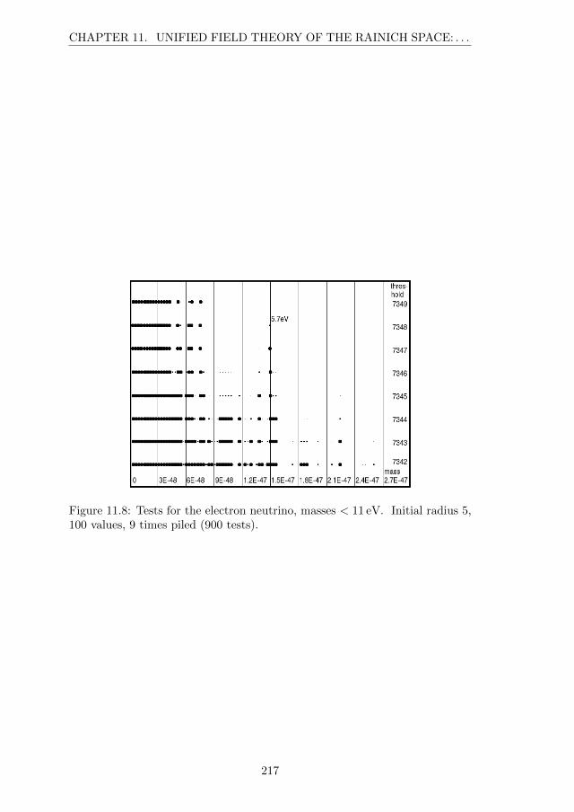
CHAPTER 11. UNIFIED FIELD THEORY OF THE RAINICH SPACE: . . .
Figure 11.8: Tests for the electron neutrino, masses < 11 eV. Initial radius 5,100 values, 9 times piled (900 tests).
217

11.8. CONCLUSION
218

Bibliography
Chapter 1 and General References
[1] M. W. Evans, H. Eckardt, D. W. Lindstrom, S. J. Crothers, “Principles ofECE Theory: A New Paradigm of Physics”, New Generation Publishingand ePubli (2016).
[2] M. W. Evans, “Generally Covariant Unified Field Theory: the Ge-ometrization of Physics” (Abramis Academic, 2005 to present), vols. 1to 4, vol. 5 in prep. (Papers 71 to 93 on www.aias.us).
[3] L. Felker, “The Evans Equations of Unified Field Theory” (Abramis Aca-demic, 2007).
[4] K. Pendergast, “Crystal Spheres” (preprint on www.aias.us, Abramis tobe published).
[5] Omnia Opera Section of www.aias.us.
[6] H. Eckardt, “ECE Engineering Model”,http://www.aias.us/documents/miscellaneous/ECE-Eng-Model.pdf.
[7] M. W. Evans, (ed.), “Modern Non-linear Optics”, a special topical issueof I. Prigogine and S. A. Rice, “Advances in Chemical Physics” (WileyInterscience, New York, 2001, second edition), vols. 119(1) to 119(3).
[8] M. W. Evans and S. Kielich (eds.), ibid., first edition (Wiley Interscience,New York, 1992, 1993, 1997), vols. 85(1) to 85(3).
[9] M. W. Evans and L. D. Crowell, “Classical and Quantum Electrodynamicsand the B(3) Field” (World Scientific, 2001).
[10] M. W. Evans and J.-P. Vigier, “The Enigmatic Photon” (Kluwer, 1994to 2002), in five volumes.
[11] M. W. Evans and A. A. Hasanein, “The Photomagneton in QuantumField Theory” (World Scientific, 1994).
[12] M. W. Evans, “The Photon’s Magnetic Field, Optical NMR” (World Sci-entific, 1992).
219

BIBLIOGRAPHY
[13] M. W. Evans, Physica B, 182, 227 and 237 (1992).
[14] S. P. Carroll, “Spacetime and Geometry, an Introduction to General Rel-ativity” (Addison Wesley, New York, 2004), chapter three.
[15] J. B. Marion and S. T. Thornton, “Classical Dynamics of Particles andSystems” (Harcourt Brace College Publishers, 1988, third edition).
[16] S. Crothers, papers and references therein on the www.aias.us site andpapers 93 of the ECE UFT series on www.aias.us.
[17] P. W. Atkins, “Molecular Quantum Mechanics” (Oxford University Press,1983, 2nd edition and subsequent editions).
[18] J. R. Croca, “Towards a Non-linear Quantum Physics” (World Scientific,2001).
[19] E. G. Milewski (Chief Editor), “The Vector Analysis Problem Solver”(Research and Education Association, New York, 1987, revised printing).
[20] J. D. Jackson, “Classical Electrodynamics” (Wiley, New York, 1999, thirdedition).
[21] M. W. Evans, Acta Phys. Polonica, 38, 2211 (2007).
[22] M. W. Evans and H. Eckardt, Physica B, 400, 175 (2007).
[23] M. W. Evans, Physica B, 403, 517 (2008).
[24] Michael Krause (Director), “All About Tesla” (a film available on DVDthat premiered in 2007).
Chapter 8
[25] T. Kambe, “On Fluid Maxwell Equations‘”, http://www.epitropakisg.gr/grigorise/T.Kambe.pdf.
[26] T. Kambe, “On Fluid Maxwell Equations” in: Sidharth B., MicheliniM., Santi L. (eds) Frontiers of Fundamental Physics and Physics Educa-tion Research. Springer Proceedings in Physics, vol 145 (2014). Springer,Cham.
[27] A. Thess et al., “Sensitivity analysis of a Lorentz force flowmeter forlaminar and turbulent flows in a circular pipe”, Center for TurbulenceResearch Proceedings of the Summer Program 2006, Stanford (2006).
220

BIBLIOGRAPHY
Chapter 11
[28] G. Y. Rainich, Electrodynamics in the General Relativity Theory. Proc.N.A.S., 10 (1924), 124-127.
[29] G. Y. Rainich, Second Note Electrodynamics in the General RelativityTheory. Proc. N.A.S., 10 (1924), 294-298.
[30] U. E. Bruchholz, Geometry of Space-Time, Progress in Physics, 5 (4)(2009), 65-66.http://www.ptep-online.com/index files/2009/PP-19-06.PDF
[31] U. E. Bruchholz, Key Notes on a Geometric Theory of Fields, Progress inPhysics, 5 (2) (2009), 107-113.http://www.ptep-online.com/index files/2009/PP-17-17.PDF
[32] A. Einstein, Grundzuge der Relativitatstheorie. A back-translation fromthe Four Lectures on Theory of Relativity. Akademie-Verlag Berlin,Pergamon Press Oxford, Friedrich Vieweg & Sohn Braunschweig (1969).
[33] L. P. Eisenhart, Riemannian Geometry, Princeton university press(1949).
[34] U. E. Bruchholz and H. Eckardt, A Numerical Method for Prediction ofMasses of Real Particles, e.g. Neutrinos, Theoretical Mathematics & Ap-plications, 6, no. 4 (2016), 53-69.http://www.scienpress.com/
[35] J. Gleick, Chaos, die Ordnung des Universums. Vorstoß in Grenzbereiche der
modernen Physik. (Engl. orig.: Chaos. Making a new science.) Droemer Knaur
Munchen (1990) ISBN 3-426-04078-6.
[36] G. Kuppers (Ed.), Chaos und Ordnung. Formen der Selbstorganisation in Natur
und Gesellschaft. Reclam Ditzingen (1996) ISBN 3-15-009434-8.
[37] A. Einstein and W. Pauli, On the non-existence of regular stationarysolutions of relativistic field equations, Ann. of Math., 44 (2) (1943), 131.
[38] U. E. Bruchholz, Masses of Nuclei Constituted from a Geometric Theoryof Fields, Adv. Studies Theor. Phys., 7 no.19 (2013), 901-906.http://dx.doi.org/10.12988/astp.2013.3885
[39] K. Hagiwara et al. (Particle Data Group), Phys. Rev. D 66, 010001 (2002)(URL: http://pdg.lbl.gov)
221

BIBLIOGRAPHY
222