principles of designing and developing spreadsheet

PRINCIPLES OF DESIGNING AND DEVELOPINGSPREADSHEET-BASED DECISION SUPPORT SYSTEMS

By

MICHELLE M. HANNA

A THESIS PRESENTED TO THE GRADUATE SCHOOLOF THE UNIVERSITY OF FLORIDA IN PARTIAL FULFILLMENT

OF THE REQUIREMENTS FOR THE DEGREE OFMASTER OF SCIENCE

UNIVERSITY OF FLORIDA

2004

Copyright 2004

by

Michelle M. Hanna

This document is dedicated to my parents for their continuous love and

support.

ACKNOWLEDGMENTS

I would like to thank Ravindra K. Ahuja for being my advisor and friend

throughout this work. I am very grateful for the opportunities he has given me to

research, write, and teach this material. I am also thankful to my fiance Onur Seref

for his constant love and encouragement.

iv

TABLE OF CONTENTSpage

ACKNOWLEDGMENTS . . . . . . . . . . . . . . . . . . . . . . . . . . . . . iv

LIST OF TABLES . . . . . . . . . . . . . . . . . . . . . . . . . . . . . . . . . viii

LIST OF FIGURES . . . . . . . . . . . . . . . . . . . . . . . . . . . . . . . . ix

ABSTRACT . . . . . . . . . . . . . . . . . . . . . . . . . . . . . . . . . . . . xiii

CHAPTERS

1 INTRODUCTION . . . . . . . . . . . . . . . . . . . . . . . . . . . . . . 1

1.1 An Introduction to DSS . . . . . . . . . . . . . . . . . . . . . . . 11.2 Defining DSS . . . . . . . . . . . . . . . . . . . . . . . . . . . . . 31.3 Excel Spreadsheets . . . . . . . . . . . . . . . . . . . . . . . . . . 61.4 VBA for Excel Programming Language . . . . . . . . . . . . . . . 71.5 The DSS Development Process . . . . . . . . . . . . . . . . . . . . 81.6 Case Studies . . . . . . . . . . . . . . . . . . . . . . . . . . . . . . 9

2 DSS DEVELOPMENT PROCESS . . . . . . . . . . . . . . . . . . . . . 10

2.1 Defining the Development Process . . . . . . . . . . . . . . . . . . 102.2 Application Overview . . . . . . . . . . . . . . . . . . . . . . . . . 112.3 Spreadsheets . . . . . . . . . . . . . . . . . . . . . . . . . . . . . . 132.4 User Interface . . . . . . . . . . . . . . . . . . . . . . . . . . . . . 182.5 Procedures . . . . . . . . . . . . . . . . . . . . . . . . . . . . . . . 282.6 Resolve Options . . . . . . . . . . . . . . . . . . . . . . . . . . . . 32

3 GUI DESIGN AND PROGRAMMING PRINCIPLES . . . . . . . . . . . 39

3.1 GUI Design . . . . . . . . . . . . . . . . . . . . . . . . . . . . . . 393.1.1 The Theory Behind Good GUI Design . . . . . . . . . . . . 39

3.1.1.1 Users, tasks, and goals . . . . . . . . . . . . . . . . . 393.1.1.2 Clarity . . . . . . . . . . . . . . . . . . . . . . . . . . 413.1.1.3 Consistency . . . . . . . . . . . . . . . . . . . . . . . 45

3.1.2 Good and Bad GUI Designs . . . . . . . . . . . . . . . . . 483.1.2.1 Buttons . . . . . . . . . . . . . . . . . . . . . . . . . 48

v

3.1.2.2 Text boxes versus list boxes and combo boxes . . . . 483.1.2.3 Tab strips and multi pages . . . . . . . . . . . . . . . 493.1.2.4 Check boxes versus option buttons . . . . . . . . . . 493.1.2.5 Frames . . . . . . . . . . . . . . . . . . . . . . . . . 513.1.2.6 Labels versus text boxes . . . . . . . . . . . . . . . . 513.1.2.7 Dynamic controls . . . . . . . . . . . . . . . . . . . . 523.1.2.8 Multiple forms . . . . . . . . . . . . . . . . . . . . . 523.1.2.9 Event procedures . . . . . . . . . . . . . . . . . . . . 54

3.2 Programming Practices . . . . . . . . . . . . . . . . . . . . . . . . 543.2.1 Consistent Style . . . . . . . . . . . . . . . . . . . . . . . . 543.2.2 Naming . . . . . . . . . . . . . . . . . . . . . . . . . . . . . 573.2.3 Comments . . . . . . . . . . . . . . . . . . . . . . . . . . . 573.2.4 Efficiency . . . . . . . . . . . . . . . . . . . . . . . . . . . . 58

4 WAREHOUSE LAYOUT . . . . . . . . . . . . . . . . . . . . . . . . . . 61

4.1 Application Overview . . . . . . . . . . . . . . . . . . . . . . . . . 614.1.1 Model Definition and Assumptions . . . . . . . . . . . . . . 614.1.2 Input . . . . . . . . . . . . . . . . . . . . . . . . . . . . . . 684.1.3 Output . . . . . . . . . . . . . . . . . . . . . . . . . . . . . 68

4.2 Spreadsheets . . . . . . . . . . . . . . . . . . . . . . . . . . . . . . 694.3 User Interface . . . . . . . . . . . . . . . . . . . . . . . . . . . . . 724.4 Procedures . . . . . . . . . . . . . . . . . . . . . . . . . . . . . . . 744.5 Resolve Options . . . . . . . . . . . . . . . . . . . . . . . . . . . . 87

5 RELIABILITY ANALYSIS . . . . . . . . . . . . . . . . . . . . . . . . . 98

5.1 Application Overview . . . . . . . . . . . . . . . . . . . . . . . . . 985.1.1 Model Definition and Assumptions . . . . . . . . . . . . . . 985.1.2 Input . . . . . . . . . . . . . . . . . . . . . . . . . . . . . . 995.1.3 Output . . . . . . . . . . . . . . . . . . . . . . . . . . . . . 100

5.2 Spreadsheets . . . . . . . . . . . . . . . . . . . . . . . . . . . . . . 1005.3 User Interface . . . . . . . . . . . . . . . . . . . . . . . . . . . . . 1055.4 Procedures . . . . . . . . . . . . . . . . . . . . . . . . . . . . . . . 1095.5 Resolve Options . . . . . . . . . . . . . . . . . . . . . . . . . . . . 121

6 CONCLUSION . . . . . . . . . . . . . . . . . . . . . . . . . . . . . . . . 128

6.1 The Importance of DSS . . . . . . . . . . . . . . . . . . . . . . . . 1286.2 Spreadsheet-Based DSS . . . . . . . . . . . . . . . . . . . . . . . . 1286.3 Developing a DSS . . . . . . . . . . . . . . . . . . . . . . . . . . . 1286.4 Conclusion and Future Direction . . . . . . . . . . . . . . . . . . . 129

vi

REFERENCES . . . . . . . . . . . . . . . . . . . . . . . . . . . . . . . . . . . 130

BIOGRAPHICAL SKETCH . . . . . . . . . . . . . . . . . . . . . . . . . . . . 131

vii

LIST OF TABLESTable page

2–1 Summary: Application Overview . . . . . . . . . . . . . . . . . . . . . 12

2–2 Summary: Spreadsheets . . . . . . . . . . . . . . . . . . . . . . . . . . 19

2–3 Summary: User Interface . . . . . . . . . . . . . . . . . . . . . . . . . 29

2–4 Summary: Procedures . . . . . . . . . . . . . . . . . . . . . . . . . . . 32

2–5 Summary: Resolve Options . . . . . . . . . . . . . . . . . . . . . . . . 37

3–1 Summary: Users, Tasks, and Goals . . . . . . . . . . . . . . . . . . . . 41

3–2 Summary: Clarity . . . . . . . . . . . . . . . . . . . . . . . . . . . . . 45

3–3 Summary: Consistency . . . . . . . . . . . . . . . . . . . . . . . . . . 48

3–4 Summary: GUI Design . . . . . . . . . . . . . . . . . . . . . . . . . . 55

3–5 Summary: Programming Principles . . . . . . . . . . . . . . . . . . . 60

4–1 Algorithm . . . . . . . . . . . . . . . . . . . . . . . . . . . . . . . . . 68









viii

LIST OF FIGURESFigure page

1–1 A schematic view of a decision support system. . . . . . . . . . . . . . 4

2–1 An example of a “Welcome” sheet. . . . . . . . . . . . . . . . . . . . 13

2–2 An example of using spreadsheets to take input from the user. . . . . 14

2–3 An example of a large set of data imported from a text file. . . . . . . 15

2–4 An example of having input, calculations, and output on the samesheet. . . . . . . . . . . . . . . . . . . . . . . . . . . . . . . . . . . 15

2–5 An example of a complicated calculations sheet. . . . . . . . . . . . . 16

2–6 An example of using a graph to illustrate results in an output sheet. . 18

2–7 An example of histograms in the output sheet of a simulation-basedDSS. . . . . . . . . . . . . . . . . . . . . . . . . . . . . . . . . . . . 19

2–8 An example of a navigational output sheet. . . . . . . . . . . . . . . . 20

2–9 An pivot table report sheet is one of the output sheets. . . . . . . . . 20

2–10 The corresponding pivot chart is another report sheet. . . . . . . . . . 21

2–11 An example of buttons on the spreadsheet to work with input andcalculations. . . . . . . . . . . . . . . . . . . . . . . . . . . . . . . . 23

2–12 An example of dynamic form controls on the spreadsheet. . . . . . . . 25

2–13 An example of controls on a form and spreadsheet. . . . . . . . . . . 26

2–14 An example of dynamic form controls. . . . . . . . . . . . . . . . . . 27

2–15 An example of a “floating” form. . . . . . . . . . . . . . . . . . . . . 28

2–16 The output sheet for the Reliability Analysis case study. . . . . . . . 34

2–17 The first resolve option: modify input in table and rerun simulation. . 35

2–18 The second resolve option: suggestion is made to aid decision maker. 36

2–19 Two “Modify” buttons give the user different resolve options. . . . . . 38

3–1 Clear instructions and descriptions on each sheet and form. . . . . . . 42

ix

3–2 Buttons are clearly separated into navigation and calculation groups. 42

3–3 Labels clearly designate functionality of controls. . . . . . . . . . . . . 43

3–4 Control tips clarify control functionality. . . . . . . . . . . . . . . . . 43

3–5 Formatting guidelines. . . . . . . . . . . . . . . . . . . . . . . . . . . 44

3–6 Clear formatting and default values. . . . . . . . . . . . . . . . . . . . 45

3–7 The navigational buttons are together and consistent in the sheet. . . 46

3–8 Consistent formatting and clear constructions. . . . . . . . . . . . . . 47

3–9 Combo boxes reduce user memorization and chance for errors. . . . . 49

3–10 Tab strips and multi pages can be replaced if too many tabs are needed. 50

3–11 Option buttons are used for mutually exclusive options and checkboxes are used for other options. . . . . . . . . . . . . . . . . . . . 51

3–12 Frames have more than one control each. . . . . . . . . . . . . . . . . 52

3–13 Labels are used for non-changeable values. . . . . . . . . . . . . . . . 53

3–14 Some functions are active and some are inactive. . . . . . . . . . . . . 53

4–1 An example warehouse layout. . . . . . . . . . . . . . . . . . . . . . . 62

4–2 The warehouse area is discretized into bay areas of value 1. . . . . . . 66

4–3 The final warehouse layout for five products and two docks. . . . . . . 67

4–4 The welcome sheet. . . . . . . . . . . . . . . . . . . . . . . . . . . . . 69

4–5 The first input sheet for dock information. . . . . . . . . . . . . . . . 70

4–6 The second input sheet for product information. . . . . . . . . . . . . 71

4–7 The output sheet with its navigational buttons and resolve options. . 72

4–8 The user form asks for the first input values. . . . . . . . . . . . . . . 73

4–9 The Main procedure and public variable declarations. . . . . . . . . . 75

4–10 The ClearPrevious procedure clears values and formatting on all sheets;it also initializes some variables. . . . . . . . . . . . . . . . . . . . . 76

4–11 The cmdOK Click procedure assigns the input values to their corre-sponding variables. . . . . . . . . . . . . . . . . . . . . . . . . . . . 77

4–12 The beginning of the NumberingBay procedure. . . . . . . . . . . . . 79

x

4–13 The end of the NumberingBay procedure. . . . . . . . . . . . . . . . . 80

4–14 The SelectionChange event procedure enables the user to click on thesheet to place the docks. . . . . . . . . . . . . . . . . . . . . . . . . 81

4–15 The DockInfo procedure records the dock information. . . . . . . . . 82

4–16 The FinalSteps procedure performs the main calculations and callthe procedures which execute the algorithm. . . . . . . . . . . . . . 83

4–17 The ComputeF procedure computes the weighted distances based onthe dock frequencies. . . . . . . . . . . . . . . . . . . . . . . . . . . 84

4–18 The SortItems procedure calculates the product type weights and sortsthem. . . . . . . . . . . . . . . . . . . . . . . . . . . . . . . . . . . 85

4–19 The SortBays algorithm sorts the bays in ascending order of theirdistance weights. . . . . . . . . . . . . . . . . . . . . . . . . . . . . 86

4–20 The beginning of the Assign procedure. . . . . . . . . . . . . . . . . . 88

4–21 The end of the Assign procedure. . . . . . . . . . . . . . . . . . . . . 89

4–22 The navigational procedures. . . . . . . . . . . . . . . . . . . . . . . . 89

4–23 The first input sheet is revisited and some of the dock information ischanged. . . . . . . . . . . . . . . . . . . . . . . . . . . . . . . . . . 90

4–24 The second input sheet is revisited and the product type informationis changed. . . . . . . . . . . . . . . . . . . . . . . . . . . . . . . . 91

4–25 The new layout is displayed after pressing the “Resolve” button. . . . 91

4–26 The resolve options allow the user to specify a particular product’slayout on the Resolve Layout grid. . . . . . . . . . . . . . . . . . . 92

4–27 The layout has been resolved with the user’s specifications enforced. . 93

4–28 Bay assignments for multiple product types can be enforced. . . . . . 93

4–29 The final layout is modified to honor the enforced bay assignments. . 94

4–30 The SelectChange event procedure allows the user to enforce particu-lar bay assignments for selected product types. . . . . . . . . . . . 96

4–31 The Resolve procedure records changes made to input values and hon-ors enforced bay assignments. . . . . . . . . . . . . . . . . . . . . . 97

5–1 An example of a parallel serial system. . . . . . . . . . . . . . . . . . 99

5–2 The welcome sheet. . . . . . . . . . . . . . . . . . . . . . . . . . . . . 101

xi

5–3 The calculation sheet for optimizing the Weibull parameters. . . . . . 102

5–4 The hidden calculation sheet for the simulation data. . . . . . . . . . 103

5–5 The simulation sheet with the animation layout and input table. . . . 104

5–6 The third calculation sheet for the results of the simulation runs. . . . 104

5–7 The top half of the output sheet. . . . . . . . . . . . . . . . . . . . . 106

5–8 The bottom half of the output sheet. . . . . . . . . . . . . . . . . . . 107

5–9 The input form with the dynamic label value for machine type “A.” . 108

5–10 The Input Box. . . . . . . . . . . . . . . . . . . . . . . . . . . . . . . 108

5–11 The Message Box. . . . . . . . . . . . . . . . . . . . . . . . . . . . . . 109

5–12 The Main procedure and variable declarations. . . . . . . . . . . . . . 111

5–13 The ClearPrev procedure. . . . . . . . . . . . . . . . . . . . . . . . . 112

5–14 The cmdOK Click event procedure. . . . . . . . . . . . . . . . . . . . 113

5–15 The CalcWeibull procedure. . . . . . . . . . . . . . . . . . . . . . . . 114

5–16 The PrepSim procedure. . . . . . . . . . . . . . . . . . . . . . . . . . 115

5–17 The beginning of the StartSim procedure. . . . . . . . . . . . . . . . . 116

5–18 The end of the StartSim procedure. . . . . . . . . . . . . . . . . . . . 117

5–19 The CreateData procedure and WeibullInv function. . . . . . . . . . . 118

5–20 The AnalysisPrep procedure. . . . . . . . . . . . . . . . . . . . . . . . 119

5–21 The navigational procedures. . . . . . . . . . . . . . . . . . . . . . . . 120

5–22 An example of the first resolve option. . . . . . . . . . . . . . . . . . 121

5–23 Updated analysis from the first resolve option. . . . . . . . . . . . . . 122

5–24 The Resolve procedure. . . . . . . . . . . . . . . . . . . . . . . . . . . 124

5–25 The resolve form. . . . . . . . . . . . . . . . . . . . . . . . . . . . . . 125

5–26 The initialization event procedure for the resolve form. . . . . . . . . 125

5–27 The Click event procedure for the ”OK” button on the resolve form. . 126

5–28 An example of the second resolve option. . . . . . . . . . . . . . . . . 127

xii

Abstract of Thesis Presented to the Graduate Schoolof the University of Florida in Partial Fulfillment of the

Requirements for the Degree of Master of Science

PRINCIPLES OF DESIGNING AND DEVELOPINGSPREADSHEET-BASED DECISION SUPPORT SYSTEMS

By

Michelle M. Hanna

August 2004

Chair: Ravi K. AhujaMajor Department: Industrial and Systems Engineering

A decision support system (DSS) is a model-based or knowledge-based system

intended to support a managerial decision making user. A spreadsheet-based DSS

uses spreadsheets to organize data and perform some spreadsheet functions. It

uses a basic programming language to design user interface and implement model

algorithms and calculations. A DSS should also offer the user some options to

resolve his problem for a comparative analysis which may enhance the decision

making process. This thesis proposes design principles and a development process

for building a spreadsheet-based decision support system.

xiii

CHAPTER 1INTRODUCTION

1.1 An Introduction to DSS

Equipped with the modeling and algorithmic skills taught in the standard

Operations Research (OR) curriculum, many industrial engineering graduates feel

ready to solve real-world problems. With a knowledge and understanding of theory

and applications of mathematical programming, simulation techniques, and supply-

chain management, they are ready to help their companies solve any distribution,

forecasting, or planning problems. But then, as they interact more with coworkers

and managers, they realize that the models they have learned cannot be applied

easily to many of the real word problems they now face.

Many of these problems are decision-making problems which require simple

solutions without the details of the mathematical models used to solve them. Most

managers would prefer a software solution for such decision problems. However,

most industrial engineering graduates know the right model but not how to

package a model and present it with a friendly graphical user interface (GUI). The

managers need to be able to easily use it, see the results with graphs or charts,

and modify inputs to analyze different business scenarios. The desired software

programs should also be able to pull data from larger databases and manipulate it

appropriately.

This is a widely prevalent problem which is not addressed in the current

OR curriculum. Models need data which is mostly available in spreadsheets or

databases. Hence, OR graduates need to know how to extract data from these

data sources. They need to know how to check data integrity and perform data

analysis and data manipulation. As OR practitioners, OR graduates are support

1

2

staff members and are required to build systems for non-OR users. They must

know how to package OR models so that they can be comfortably used by top

managers and other co-workers. Real-life decision making often requires building

interactive systems, which OR graduates must know how to design and implement.

To summarize, OR graduates must learn sufficient information technology skills to

that they can build intelligent information systems, alternatively, called decision

support systems, which can run sophisticated models at the back-end, but are

friendly enough at the front end to be used comfortably by any user.

A decision support system (DSS) gives its users access to a variety of data

sources, modeling techniques, and stored domain knowledge via an easy to use

GUI. For example, a DSS can use the data residing in spreadsheets, prepare a

mathematical model using this data, solve it or analyze it using problem-specific

methodologies, and assists the user in the decision-making process through a

graphical user interface. The importance of DSS development skills has become

well noted in the literature: “Given the growing complexity and uncertainty in

many decision situations, helping managers use quantitative models to support

their decision making and planning is an important research topic” ( [1]). DSS

applications are usually intended to be designed for non technical users presented

with an easy to use interface.

OR graduates are frequently being employed in positions that require devel-

oping DSS which are gaining widespread popularity. As more and more companies

install enterprise resource planning (ERP) packages and invest in building data

warehouses, those who are able to create decision technologies driven applications

that interface with these systems and analyze the data they provide will become

increasingly valuable. Indeed, imparting DSS development skills, which combine

OR skills with IT skills, will make graduates highly sought after in the modern

workplace.

3

Developing courses that teach OR students how to build DSS has been a

challenging task so far since it requires the availability of platforms which allowed

the integration of various technologies (data, models, codes, etc.). However, in

the past few years, several platforms have become available which allows such

integration. One such platform is Microsoft Excel. Excel, which is the most widely

used spreadsheet package among managers and engineers, allows data storage and

model building. Excel also has many built-in program as well as many add-on

programs available that wallow optimization and simulation of various models

built in Excel. Excel also has a macro programming language, Visual Basic for

Applications (VBA), which allows building GUIs and manipulating Excel objects.

Thus, Excel provides a platform using which fairly sophisticated DSS applications

can be built.

1.2 Defining DSS


intended to support managerial decision making. A DSS is not meant to replace a

decision maker, but to extend his/her decision making capabilities. It uses data,

provides a clear user interface, and can incorporate the decision maker’s own

insights. Some of the major DSS capabilities are the following.

1. A DSS brings together human judgment and computerized information forsemi-structured decision situations. Such problems cannot be convenientlysolved by standard quantitative techniques or computerized systems.

2. A DSS is designed to be easy to use. User friendliness, graphical capabilities,and an interactive human-machine interface greatly increase the effectivenessof a DSS.

3. A DSS usually uses models for analyzing decision-making situations and mayalso include a knowledge component.

4. A DSS attempts to improve the effectiveness of decision making rather thanits efficiency.

4

User

GUI

Knowledge Base Database Model Base

Figure 1–1: A schematic view of a decision support system.

5. A DSS provides support for various managerial levels from line mangers totop executives. It provides support to individuals as well as groups. It can bePC-based or

A DSS application contains five components: database, model base, knowledge

base, GUI, and user (see Figure 1.1). The database stores the data, model and

knowledge bases store the collections of models and knowledge, respectively, and

the GUI allows the user to interact with the database, model base and knowledge

base. We now present a more detailed look at each of these components.

Database The database provides the data with which decisions are made. The

data may reside in spreadsheets or a data warehouse, a repository for

corporate relevant decision-making data. The database allows a user to

access, manipulate, and query data. Some examples of databases would

include a spreadsheet containing personal banking account information or a

data warehouse containing shipment records of various products.

Model Base A model base contains statistical, financial, optimization, or simu-

lation models that provide the analysis capabilities in a DSS. Some popular

5

optimization models include linear programming, integer programming, and

nonlinear programming. The DSS allows the ability to invoke, run, and

change any model or combine multiple models. An example of a model base

would be an integer programming model used to solve a capital budgeting

problem. Most common DSS applications are primarily model driven. A key

DSS component is its resolve options. A user should be able to manipulate

their input values to compare multiple results for scenario analysis. The DSS

should be designed for repeated use to aid in a recurring decision situation. It

should be dynamic enough to handle various problem sizes, input values, and

objectives.

Knowledge Base Many managerial decision making problems are so complex

that they require special expertise for their solution. The knowledge base

part of a DSS allows this expertise to be stored and accessed to enhance the

operation of other DSS components. For example, credit card companies

use a DSS to identify credit card thefts. They store in their knowledge base

the spending patterns that usually follow credit card thefts; any abnormal

activity in an account would trigger checking for the presence of those patters

and a possible suspension of the account.

GUI The graphical user interface (GUI) covers all aspects of communication

between a user and a DSS application. The user interface interacts with the

database, model base, and knowledge base. It allows the user to enter data

or update data, run the chosen model, view the results of the model, and

possible rerun the application with different data and/or model combination.

6

The user interface is perhaps the most important component of a DSS

because much of the poser, flexibility, and ease of use of a DSS are derived

from this component.

User The person which use the DSS to support the decision making process is

called the user, or decision maker. A DSS has two broad classes of users:

managers and staff specialists, or engineers. When designing a DSS, it is

important to know for which class of users the DSS is being designed. In

general, managers expect a DSS to be more user-friendly than do staff

specialists.

A DSS should be distinguished from more common management information

systems (MIS). An MIS can be viewed as an information system that can generate

standard and exception reports and summaries for managers, provide answers to

queries, and help in monitoring the performance of a system using simple data

processing. A DSS can be viewed as a more sophisticated MIS where we allow the

use of models and knowledge bases to process the data and perform analysis.

1.3 Excel Spreadsheets

Microsoft Excel spreadsheets have become one of the most popular software

packages in the business world, so much so that business schools have developed

several popular Excel based courses. A spreadsheet application has functionality for

storing and organizing data, performing various calculations, and using additional

packages, called Add-Ins, for more advanced problem solving and analysis. Excel

spreadsheets are easy for a user to interact with and easy for a student to use

7

while developing the DSS. We consider two aspects of Excel to be important in

developing a DSS: basic functionality and extended functionality.

Excel basic functionality includes referencing and names, functions and

formulas, charts, and pivot tables. These are standard tools that may be common

to most spreadsheet users. Excel extended functionality includes statistical

analysis, the Solver and modeling, simulation, and querying large data. These

tools are especially important for building a decision support system. The ability

to model a problem and solve it or simulate it adds the model base component of

the DSS we are building. It is important that a DSS developer become familiar

with the capabilities of Excel so that they know what they can offer the user when

developing a decision support system.

1.4 VBA for Excel Programming Language

VBA for Excel is a programming language that allows for further manipulation

of the Excel functionalities. VBA for Excel also allows the developer to create

dynamic applications which can receive user input for the model base component

of the DSS. VBA allows users without knowledge of Excel to be able to use

spreadsheet-based DSS applications. There are several important features of VBA

for Excel.

Some of these features include recording macros and working with variables,

procedures, programming structures, and arrays in VBA. VBA for Excel is an

easy to understand programming language. Even if a student has not programmed

8

before, they should be able to program several types of applications after a basic

introduction to VBA.

A DSS developer can also create a user interface in VBA. These features

includes building user forms, working with several different form controls, using

navigational functions, and designing a clear and professional application. VBA is

beneficial as it places all of the complicated spreadsheet calculations and any other

analysis in the background of a user-friendly system.

Some of the extended Excel functionality topics can be further enhanced by

using VBA. The modeling, simulation, and query features of Excel can become

dynamic using VBA commands. These techniques are especially important to

understand in order to build complete DSS applications.

1.5 The DSS Development Process

We present a chapter on the DSS development process to explain how the

Excel spreadsheet functionality and VBA programming features can be combined

to develop a complete DSS application. We propose five basic steps for this

development process: i) outlining the application, its model and assumption;

ii) determining how many spreadsheets will be needed and for what purposes;

iii) constructing a general layout of the user interface features; iv) outlining

the programming procedures needed; and v) ensuring that resolve options will

be integrated into the DSS. We describe these steps in detail and give several

examples in this chapter.

9

We also present a chapter on GUI design and programming principles. There

is much literature on these two topics which are important in developing any DSS.

We summarize the issues that are most relevant to developing spreadsheet-DSS

applications in this chapter.

1.6 Case Studies

We present two case studies to illustrate the relevance and importance of

decision support systems in the fields of industrial and systems engineering and

business. We strive to accomplish this by showing how to develop DSS applications

which integrate databases, models, methodologies, and user interfaces.

These case studies consist of developing a complete decision support system

and are based on an important application of IE/OR or business. Through case

studies, graduates will learn how IE/OR and business techniques apply to real-life

decision problems and how those techniques can be effectively used to build DSS

applications.

These case studies are just some of the numerous case studies we develop in

order to illustrate how DSS applications can be developed by combining informa-

tion technology tools with operations research and business tools to solve important

decision problems.

CHAPTER 2DSS DEVELOPMENT PROCESS

2.1 Defining the Development Process

Now that we have discussed in great detail the components of a spreadsheet-

based decision support system (DSS), we need to learn the process of putting these

components together to build a complete DSS application. Before entering formulas

into Excel or coding sub procedures in VBA, it is necessary to construct an overall

layout for the DSS and give some thought to the design and implementation of

the application. We propose five basic steps for developing a DSS: i) Application

Overview: create a layout of the entire application to understand the flow from the

user input to the model calculations to the output, ii) Spreadsheets: determine how

many spreadsheets you will need to best handle input, calculations, and output,

iii) User Interface: outline what interface you will need to receive input from the

user and navigate them through the application, iv) Procedures: outline what sub

and/or function procedures you will need in your code to receive the input, perform

the calculations, and display the output, v) DSS Components: decide what resolve

options the user may have.

These steps have been our guidelines to developing decision support systems.

We do not claim that they are necessary to follow, but rather suggest them as

good guidelines when developing a DSS application. In this chapter we give

several examples from case studies we have developed using these proposed

steps. The following chapters give a more detailed explanation of each case

study’s development using these five steps. We wish to illustrate the variety, and

consistencies, possible in developing DSS applications.

10

11

2.2 Application Overview

The Application Overview is the most important step in developing a DSS.

In this step, we consider the entire flow of the application. We usually begin this

flow at the “Welcome” sheet. A “Welcome” sheet should have the title of the DSS

and some description of what the application does. Any assumptions or necessary

model explanations may be given in this description. There may also be some

images on this initial sheet related to the application topic. Then there should be

one button to “Start” or “Begin” the application. Even though this sheet is simple,

it is an important introduction for the user to what your DSS is and how they can

begin to use it.

The user should then encounter some method for providing input. This may

involve a form or set of forms, or the user may be brought to a new sheet where

further instructions are provided. Deciding which method or methods to use is

important and depends on the application. For example, if you only need one or

two pieces of information from the user, you may not even need a form or an entire

sheet for input; instead, you may use an Input Box. In some applications, you may

need large sets of data for your analysis. In that case, you may only prompt the

user to import data from a text file or database to a spreadsheet. Once you have

decided which method is most appropriate for your application, you may need

to spend more time designing the interface; however, we will return to this in a

later step. It is important to complete the Application Overview before designing

the interface so that you have a clear idea of what the entire application will

incorporate.

After receiving the input, the model should be ready and calculations can be

performed. It is a good idea at this point to have an overview of what is required

for your model calculations. You may need to know the model formulation before

you can finish deciding what the user input will be. The first thing to decide is

12

if this DSS will be computing simple calculations, performing an optimization,

or running a simulation. The details of these models can be outlined in a later

step, but for the purpose of the Application Overview, you should have an idea

of what will be involved. This general model outline will help you in determining

the details of your spreadsheet design and procedures later. Once input is received

and the model calculations are performed, we need to determine what output will

be displayed to the user. Will there be charts or graphs, or histograms or tables?

Does some of the input need to be re-displayed to the user? Again, these options

will depend on the application. It is important to consider the output as it is a

driving force in why the user is using the DSS. It is a good check to see if you are

computing everything the user may be interested in.

The last part of the Application Overview is reviewing the DSS components.

In Chapter 1, we define in detail what a DSS is comprised of. These include, the

model base and user interface discussed above. However, a DSS should also provide

some resolve options for the user. The user should be able to change some of their

initial input values and resolve the problem. The user may also want to add some

constraints to an optimization or redefine their objective function. We suggest that

these resolve options are made available on the output sheet. We will give more

examples of these DSS components in the following sections.

Table 2–1: Summary: Application Overview

Welcome Sheet Flow begins; introduction to what DSS is and how tobegin using it.

Input Provided by user via set of forms, input spreadsheet, orInput Boxes.

Model Calculations Formulation of objectives and necessary input; decide ifcomputing simple calculations, performing an optimiza-tion, or running a simulation.

Output A driving force in why the user is using the DSS.Resolve Options Use can modify input, redefine constraints, or change

objectives.

13

Figure 2–1: An example of a “Welcome” sheet.

2.3 Spreadsheets

There may be two to several sheets in a DSS application. The first sheet

should always be the “Welcome” sheet as we discussed above. For example, in

Figure 2.1, we show the “Welcome” sheet from a case study we developed for a

Portfolio Management and Optimization DSS. We give a description of the DSS

and describe the model assumptions. We also reference the source of our model

formulation. We also have some images related to portfolios. Then we have a

“Start” button which the user can press to begin the application.

The remaining sheets are for input, calculations, and output. We may have

these as separate sheets or some elements may be combined on fewer sheets. Sup-

pose we need a sheet for input. We can prepare the sheet by placing appropriate

labels for tables or input locations. We may also name some ranges at this point

which will help us later when coding. Below is an example from a case study we

14

Figure 2–2: An example of using spreadsheets to take input from the user.

developed for using the Critical Path Method (see Figure 2.2). In this application,

we take the user through several input sheets. In each sheet, we have a table for a

set of input values. In some cases, spreadsheet may be a better user interface than

forms for receiving input; we discuss this in more detail in the next section.

You may also have an application which requires a large set of data. This data

may be imported from a text file or database, or input by the user. In Figure 2.3,

we have an input sheet from a Stochastic Customer Forecasting case study. This

sheet contains the historical data that is used to make future forecasts. In this

application we give the user the option to enter this data manually or import it

from a text file.

You may not need an input sheet for every application. Let us consider the

case where the input sheet may be combined with the calculations sheet or output

sheet. For example, in the figure below, we have a sheet from a Technical Analysis

case study in which the input, calculations, and output are all on one sheet (see

Figure 2.4). Here the user can modify the input using spreadsheet controls and

press the “Resolve” button to update the calculations in the table. The output is

summarized in a small table on the right of the screen.

Again, you may not even use a sheet at all for your input. You may simply

take input from a user form and then use that directly in a calculations sheet or

15

Figure 2–3: An example of a large set of data imported from a text file.

Figure 2–4: An example of having input, calculations, and output on the samesheet.

16

Figure 2–5: An example of a complicated calculations sheet.

in some calculations procedures and take the user directly to the output sheet.

Since we are developing spreadsheet-based DSS applications, we will usually take

advantage of the spreadsheet features to aid us in performing calculations. For this

reason, we will usually have a calculations sheet. This sheet may be viewed by the

user or, in most cases, hidden from the user. A calculations sheet should be hidden

if the intended user may not be familiar with the details of the calculations but is

solely interested in the results. In Figure 2.5, we have a complicated calculations

sheet from a simulation performed in a Retirement Planning case study. There are

several spreadsheet functions and formulas in the sheet as well as some input cells

whose values have been updated after a user has completed an input form. Since

the sheet calculations are somewhat complicated, we do not show this sheet to the

user during the normal flow of the application; however, we do give the user the

option to view the calculations if they want to. We normally, take the user directly

from the input form to the output sheet in this application.

17

You may have some other hidden sheets related to the calculations. For

example, in simulation we usually store the results of the runs to user for creating

histograms or other summary reports. This detailed sheet should be hidden

from the user in the application flow, but can be made available for viewing if

the user is interested. By using the Application.ScreenUpdating method and

Worksheets.Visible property we can prevent the user from seeing these calculation

sheets while they are being used for the model calculations. Probably the most

important sheet for the user is the output sheet. This sheet should summarize the

results of the calculations clearly so that the user can understand the behavior of

whatever system they were modeling or analyzing. It is usually a good idea to have

some graphical results as part of the output sheet. For example, in Figure 2.6, we

have the results sheet from an Inventory Management case study. Here the graph

illustrates the ordering strategy found by the model calculations. There are also

some tables used to summarize the numerical results of the solution.

In DSS applications using simulation, it is usually good to have some his-

tograms as part of the output sheet. In Figure 2.7, we have some histograms

summarizing the results of a Reliability Analysis case study. We have a histogram

showing the frequency of various system failure time values using a bar graph along

with an overlaid scatter plot to show the cumulative probability of each value.

Below that, we have another histogram representing the frequency with which

different machine types have caused the system failure; this histogram is shown as

a pie chart. We give the user several options from this output sheet including to

return to and rerun the simulation or return to the initial input phase to resolve

the problem.

In some cases, you may have several charts or larger summary tables that may

not fit into one output sheet. In that case, we recommend making a navigational

output sheet which will allow the user to view these individual reports. For

18

Figure 2–6: An example of using a graph to illustrate results in an output sheet.

example, In Figure 2.8, we show a navigational output sheet from a Supply Chain

Management case study. This sheet allows the user to view several different

summary pivot tables (see Figure 2.9). From these pivot tables, the user can also

view corresponding pivot charts displayed as separate chart sheets (see Figure

2.10). The user can always return to the navigational output sheet from any of

these reports.

Whichever results are relevant to your application, you should ensure that they

are presented to clearly in the output sheet. “End” and “Resolve” options should

also be found in the output sheet as well as options to “View” input or calculation

sheets.

2.4 User Interface

Designing a user interface is an important element of developing a user-

friendly DSS. We discuss good graphical user interface (GUI) design in a later

section; for now we will discuss what role the user interface plays in the DSS

development. There are three main categories of user interface in spreadsheet-based

19

Figure 2–7: An example of histograms in the output sheet of a simulation-basedDSS.

Table 2–2: Summary: Spreadsheets

Welcome Sheet Title and description of the DSS; images; “Start” but-ton.

Input Sheet User input; large data input; can be combined withother sheets.

Calculations Sheet Spreadsheet calculations; simulation results; usuallyhidden from user.

Output Sheet Summary tables and reports; graphs, charts or his-tograms; navigational output buttons; “End,” “Re-solve,” and “View” buttons.

20

Figure 2–8: An example of a navigational output sheet.

Figure 2–9: An pivot table report sheet is one of the output sheets.

21

Figure 2–10: The corresponding pivot chart is another report sheet.

DSS applications: user forms, form controls on the spreadsheet, and navigational

buttons on the spreadsheet.

Let us begin by discussing navigational buttons. As we have already men-

tioned, the first button you should create is the “Start” button which is located on

the “Welcome” sheet (see Figure 2.1). This button should be assigned to a macro

which brings the user to the input interface. On all other sheets, input, calculation,

and output sheets, there should at least be an “End” button. The user should

always have the option to “End” or “Exit” the application. Note: Whether you use

“End” or “Exit” or any other phrase for this action, be sure that you are consistent

across all sheets in the application. We discuss consistency in user interface design

more in the GUI design section.

You may also have some other navigational buttons such as “Next,” “Con-

tinue,” or “Back” if you intend for the user to be able to step through the sheets or

revisit sheets. This is especially important if you have hidden the sheet tabs or are

22

only making one sheet visible at a time; which we recommend for a more profes-

sional presentation. In the case where input, calculations, or output are combined,

you may also have some functional buttons on the spreadsheet such as “Solve.”

For example, in Figure 2.11, we have one such sheet in a case study on the

Animation of the Kruskal Algorithm. In this case study, we take the user directly

from the “Welcome” sheet to the sheet shown in the figure. We highlight the

“Create Table” button as it the next button they should press (see Figure 2.11(a)).

When they press this button, they are prompted to give the dimensions of their

network, and then a table with the corresponding number of rows is created. After

the table is created, we now make a new button visible called “Solve” (see Figure

2.11(b)). We un-highlight the “Create Table” button and highlight the “Solve”

button since this is the next button the user should click. This button will run the

procedure which animates Kruskal’s algorithms and finds the minimum spanning

tree solution.

Aside from using functional or navigational buttons on the spreadsheet, a

user interface may also use form controls on the spreadsheet. Refer to Figure 2.4

to see an example of text boxes and combo boxes used on a spreadsheet in which

input was taken from the user on the same sheet where calculations and output

were displayed. Another example is shown in Figure 2.12. This example is from the

Inventory Management case study. Here we have three option buttons representing

different methods which can be used to find the best order strategy. These option

buttons are mutually exclusive and two of them also have dynamic features. The

bottom two buttons have some associated cells for extra input which are shaded

darker when unmarked and made lighter when marked (see Figure 2.12(b)).

Form controls on the spreadsheet are useful when there are many resolve

options in the application. In this case, you want to give the user easy access to the

input in order to be able to change it multiple times. It is important to keep the

23

(a)

(b)

Figure 2–11: An example of buttons on the spreadsheet to work with input andcalculations.

24

layout of the spreadsheet clear and uncluttered when using placing form controls

adjacent to other input cells, calculations, or output. We discuss these interface

design issues in a later section.

In some cases, there may be an even tradeoff between using functional buttons

or form controls on the spreadsheet versus creating a user form. For example,

in Figure 2.13(a), we have used two functional buttons to allow a user to “Add”

and “Remove” stocks to and from their portfolio in the Portfolio Management

and Optimization case study. In this particular case study, we have put this

functionality on the spreadsheet because it is a feature the user may use often. The

user may go to a new sheet to view stock comparisons and then return to edit their

portfolio; the user may also go to an optimization sheet to view investment strategy

results and then return to edit their portfolio and resolve. However, if this were not

the case, that is if the user did not need to create or edit their portfolio multiple

times, we may have created a user form to perform this functionality. In Figure

2.13(b), we show an example of such a form used in a Beta of Stocks case study. In

this case, the user only selects their portfolio once.

In most DSS applications, if there is a large enough set of input required

from the user, we suggest creating user forms. User forms can be advantageous in

that there are many options for placing and manipulating controls on a user form.

The controls can also be more clearly displayed as they are not interfering with

other cells on the spreadsheet. Another advantage of user forms is that they can

be displayed to the user at any time; that is, they are not attached to a specific

spreadsheet. This can be especially useful for resolve options.

If a user wishes to resolve the problem and presses a “Resolve” button on an

output sheet, the input form can be redisplayed to them directly without even

moving to a new sheet. In Figure 2.14, we have an example of a user form from a

Retirement Planning case study. This form is dynamic in that the first frame below

25

(a)

(b)

Figure 2–12: An example of dynamic form controls on the spreadsheet.

26

(a)

(b)

Figure 2–13: An example of controls on a form and spreadsheet.

27

(a) (b)

Figure 2–14: An example of dynamic form controls.

the text boxes may change depending on a previously selected option. In Figure

2.14(a), the user is providing values for “Desired Savings at Retirement” and

“Confidence Interval for Returns” whereas in Figure 2.14(b) this framed is changed

to prompt the user for the “Age to Retire.” The second frame on this form, for

“Asset Allocation,” is also dynamic. In Figure 2.14(a) the user is prompted to

enter this information, but in Figure 2.14(b) the textboxes are grayed and locked

since the information is not relevant for this option.

Another way to use user forms in a situation where the user may need to

modify input multiple times is to create a “floating” form. The advantage of this

type of user form is that the user can select or modify cells in the spreadsheet

without having to close the form first. In Figure 2.15, there is an example of a

floating form from a case study for Animating the Simplex Method. This form is

used to allow the user to select the entering variable for each iteration. The user

selects the entering variable from the tableau on the spreadsheet and can then view

28

Figure 2–15: An example of a “floating” form.

the results for that scenario on the floating form. The form is hidden when the user

moves to another sheet.

2.5 Procedures

The next step in developing a DSS application is to make an outline of what

procedures you will need to conduct the flow and execute the calculations. As

discussed in Chapter 15, we encourage you to organize your code into several

smaller procedures which may be called from other main procedures or associated

with buttons on the spreadsheet. We recommend making an outline of these

procedures in your code before you begin the details of the implementation. We

always begin our applications with a Main sub procedure which is associated with

the “Start” button on the “Welcome” sheet. From the Main procedure, we usually

29

Table 2–3: Summary: User Interface

Navigational But-tons

These buttons, such as “Start,” “Next,” “Back,” or“End” should be on every sheet to navigate the userthrough the application.

Functional Buttons These buttons, such as “Create Table” or “Solve,” maybe used if multiple functions occur on one sheet.

Controls on theSpreadsheet

Placing controls on the spreadsheet allows users toeasily modify input for multiple solution calculations.

User Forms User forms are most commonly used when largeamounts of input are needed; they are often advan-tageous.

begin by clearing previous data and initializing variables; this can also be done by

calling a ClearPrevious procedure. We then either take the user to an input sheet

or show them an input form. Consider the following example.

Sub Main()

Call ClearPrevious

frmInput.Show

Worksheets(‘‘Input").Visible = True

Worksheets(‘‘Welcome").Visible = False

End Sub

Sub ClearPrevious()

’clear ranges on other sheets

Worksheets(‘‘Calc").Range(‘‘InputValues").ClearContents

Worksheets(‘‘Output").Range(‘‘Results").ClearContents

’initialize variables

Set InputRange = Worksheets(‘‘Input").Range(‘‘InputStart")

End Sub

30

There should then be some procedure which receives the input from the user.

If we are using user forms as the interface for receiving input, then this code would

be in the event procedures for the form. Consider the following example.

Sub cmdOK_Click()

’set variables equal to control values

NumRuns = txtNumRuns.Value

InputSize = txtInputSize.Value

ReDim InputArray(InputSize)

Unload Me

End Sub

Once the input is received, the calculations should be ready to perform. These

calculations may involve running a simulation with some loop structure or evoking

the solver with the Solver commands. The calculation procedure/s may be called

when the “OK” button is clicked on a user form or they may be assigned to a

“Solve” or “Continue” button on an input spreadsheet. Consider the following

example.

Sub DoSimulation()

For i = 1 to NumRuns

’create random values

’perform calculations

Next i

End Sub

Sub DoOptimization()

SolverReset

SolverOK SetCell:= , MaxMinVal:= , ByChange:=

SolverAdd CellRef:= , Relation:=, FormulaText:=

31

SolverOptions AssumeNonNeg:=True

SolverSolve UserFinish:=True

End Sub

The final procedure to be outlined is related to displaying the solution on the

output sheet. If there is a chart, you may need to update the source data. If there

was a simulation, you may want to create some histograms. In any case, you want

to put the solution values in some report table on the output sheet. The procedure

to create the output may be called from the calculation procedures or from another

functional or navigational button on the calculation spreadsheet. Consider the

following example.

Sub CreateReport()

’place solutions in report table

’update chart source data

ActiveSheet.ChartObjects(1).Select

ActiveChart.SetSourceData Source:=

’create histogram

Application.Run ‘‘ATPVBAEN.XLA!Histogram," Input, Output, Bin, Labels,

Pareto, Cumulative, Chart

Worksheets(‘‘Output").Visible = True

End Sub

These procedures should outline the overall flow of the application from user

input to calculations to output. Aside from these, there should also be any needed

navigational procedures for “End” buttons or “Next,” “Back,” or “View” buttons.

Consider the following example.

Sub EndProgram()

Worksheets(‘‘Welcome").Visible = True

32

ActiveSheet.Visible = False

End Sub

Also ensure that all variables are declared and that any variables used in

multiple procedures are declared as Public variables at the top of the module.

Table 2–4: Summary: Procedures

Main Call ClearPrevious procedure. Show input form or takeuser to input sheet.

Clear Previous Clear previous ranges of input or solution values. Ini-tialize variables.

Receive Input Store values from form controls or input cells to corre-sponding variables. Record these values to appropriatecells in calculation sheet.

Perform Calcula-tions

Perform calculations using function procedures, simula-tions loops, or Solver commands.

Generate Output Display solution values to report table, update chartsource data, or create histograms.

Navigational Change Visible property of worksheets for “End,”“Next,” “Back,” or “View” button functionality.

Variables Make sure all variables are declared and that variablesused in more than one procedure are declared as Publicvariables at the top of the module.

2.6 Resolve Options

The last but most important step in developing a DSS application is to ensure

that it has all of the components of a complete decision support system. There

should be some input taken from the user via some GUI, and there should be some

calculations made based on some model base, database, or knowledge base. We

confirm the input interface while outlining the user interface, and we confirm the

calculations and model in the procedure outline. The other important DSS feature

that we should now check is the resolve options.

Can the user easily modify the input to resolve the problem without having to

re-enter all input from scratch? We should ensure that this is possible by making

sure the user’s initial input values are preserved when re-displaying a user form

33

or input sheet. Make sure you do not call a ClearPrevious procedure unless the

user has indeed restarted the entire application. Also ensure that default values

do not overwrite the user’s last input values when re-showing a user form. This

allows users to quickly modify one or several parts of the input and resolve the

calculations to compare results.

Can the user change other parts of the calculations or model when resolving?

That is, we do not want the user to be limited to only modifying input values when

resolving. The user should be able to change some constraints or objectives as well.

Try to keep your application dynamic so that a user can experiment with different

problem dimensions. This may not be possible or applicable for every DSS, but

if it is, it should be made available to the user. If some dynamic options are not

available to the user, state your assumptions clearly on the “Welcome” sheet to

explain this.

With resolve options, you may want to provide the user with a way to compare

various results or scenarios. You may want to store multiple solutions for this

comparison or sensitivity analysis. Ask yourself what the user is really interested in

learning from the DSS. Remember that a DSS is designed to aid a decision maker

in making a decision. Check that the results of the application are indeed helpful to

this decision making process.

We will give a few examples from our case studies; a detailed description of

the DSS components can be found in each case study chapter in this part of the

book. Let us first consider the Reliability Analysis case study. In this study, a

user is analyzing a parallel series system of three machine types. After providing

the necessary input, a simulation is run to determine the mean failure time of the

system and how often a particular machine type caused the system failure. Figure

2.16 shows the output sheet for this study.

34

Figure 2–16: The output sheet for the Reliability Analysis case study.

35

Figure 2–17: The first resolve option: modify input in table and rerun simulation.

In this case, we have two resolve options for the user. The first option is for

the user to return to the simulation sheet and modify the initial input values in a

given table (see Figure 2.17). They can then re-run the simulation and view the

updated results.

The second option is for the user to improve the system by adding one

machine of a particular machine type. To aid the user, or decision maker, in

deciding which machine type they should add a machine to, we first run an

optimization in the background and suggest to them the optimal choice. We do not

enforce this decision, but instead try to aid the decision maker. This information is

presented to the user on a user form (see Figure 2.18).

After a machine type is selected, one machine is added to this type and the

simulation is rerun. The updated results are then shown.

36

Figure 2–18: The second resolve option: suggestion is made to aid decision maker.

Another example is from the Inventory Management case study (refer to

Figure 2.12). In this case, the user can actually change the model base along

with the input each time the application is resolved. The user can decide which

inventory model to use: Standard EOQ, Backorders, or Reorder Point. There is

also an input table which can be modified on the same sheet.

Another example is from the Portfolio Management case study (refer to Figure

2.13). In this case, after the user has created their portfolio, they can optimize

their investment strategy by minimizing risk (see Figure 2.19).

After filling the input in the user form for the optimization (Figure 2.19(a)),

the resulting optimized investment strategy is displayed on an output sheet

(Figure 2.19(b)). However, if the optimization was infeasible, or if the user wants

to experiment with different values, they can either return to the input form to

experiment with different values (by pressing the “Modify Input” button), or return

to the portfolio sheet to modify their stock selection (by pressing the “Modify

37

Portfolio” button). An extension to this case study may be to allow the user to

modify their objective in optimizing their investment strategy; currently we assume

that we minimize risk, but the user may also want to maximize returns.

Resolve options are an important DSS component. Ensure that the DSS is

aiding the decision maker by allowing the user to modify inputs or calculation

options.

Table 2–5: Summary: Resolve Options

Resolve Options Modify inputs, calculation options, constraints, objec-tives; aid decision maker in making the best decision.

38

(a)

(b)

Figure 2–19: Two “Modify” buttons give the user different resolve options.

CHAPTER 3GUI DESIGN AND PROGRAMMING PRINCIPLES

3.1 GUI Design

A graphical user interface (GUI) is the “graphical representation of, and

interaction with, programs, data, and objects on a computer screen.” (Mandel [2])

It presents a visual display of information and objects which can present visual

feedback to a user. Part of the definition of a DSS is: A DSS is designed to be easy

to use; user friendliness, graphical capabilities, and an interactive human-machine

interface greatly increase the effectiveness of a DSS (refer to Chapter 1). Thus, it

is very important to design the user interface such that it is easy for the user to

understand and use. If the user interface is not designed well, then the application’s

functionality will not be appreciated. In this section, we will discuss some theory

behind good GUI design and give some examples of good and bad user interfaces.

3.1.1 The Theory Behind Good GUI Design

There are many GUI design books which lists several different principles and

guidelines for good GUI design. We present here a summarized version of what we

feel are the most important theoretical points for good GUI design in spreadsheet-

based DSS applications. These are: knowing the user, the user’s tasks and goals;

maintaining clarity, and staying consistent.

3.1.1.1 Users, tasks, and goals

It is important to know who the users of your application will be. Are they

managers? If so, how deep is their understanding of the problem? Do they know

the model or algorithms being used to perform the calculations? What terminology

do they use to discuss the problem? If the user does not have a highly technical

understanding of the topic of the application, then try to avoid describing the

39

40

details of the model or calculations. This would be a case when the calculation

sheet may remain hidden. Try also to give instructions and label input without

using technical terminology. For example, instead of labeling input as C or D, give

meaningful descriptions such as “Annual Cost” or “Annual Demand.” In the case

that your users do have a more technical understanding, you should show and

explain the calculations and assumptions. You may also want to give more details

using the terminology they are familiar with.

Keep in mind that the user is using this application to complete some tasks

and achieve a goal. It is important to ensure that the user interface is an aid to

the user in completing these tasks so that the user feels that the DSS has indeed

become a helpful tool in increasing the efficiency of achieving their goal. The

user’s task domain includes “the data that users manipulate, the manner in which

that data is divided , and the nature of the manipulation that users perform on

the data.” (Johnson [3]) Remember that the user’s tasks are already necessary

without the help of a DSS; therefore, ensure that your DSS application aids them

in completing these tasks in the same domain they are familiar with. These tasks

should be organized on some priority or hierarchy base in order to create a flow

for the application. This flow influences the outline of the entire application as

we discussed in the first section. Your interface should guide the user so that they

can work with the data in their task domain in the order in which it needs to be

completed.

For example, let us suppose that the user’s task domain involves looking

at some historical data, then computing a mean and standard deviation of this

data, and then entering these values into a forecasting model. Based on the result

of the model, the user has to take the forecast demand for the next month and

place an order of that size. When constructing the interface for a forecasting DSS,

ensure that these tasks are presented to the user in the same order. First, ask

41

them to enter the historical data. If they usually get this data as a text file from

a coworker, then do not ask them to enter it manually, instead prompt them to

import the text file. You can then automatically calculate the mean and standard

deviation to display for them. Afterwards you may ask for some extra input for

the forecasting model, but try not to get to technical. You may then display

clearly to them what their order amount should be based on this forecast. Do not

try to reorganize their tasks as they will find the DSS hard to learn. Keep the

presentation of the tasks simple so that there is an element of familiarity for them.

Table 3–1: Summary: Users, Tasks, and Goals

What is the user’s knowledge of the problem and technical understanding ofthe model calculations?What terminology is the user familiar with?Define the user’s task domain to determine the application flow.

3.1.1.2 Clarity

A user interface is the communication between the user and the application;

therefore, if you want the user to use the application correctly, you must communi-

cate clearly to them what they should do to use it. First and foremost, make sure

there is a clear description of what is involved on every spreadsheet and every form.

For example, in Figure 3.1, we show the calculation sheet from a Sales Force Allo-

cation case study. We ask the user to enter some bound values for the optimization

constraints. We then give them two calculation options. We explain the user’s

tasks in a text box at the top of the sheet. We have bolded the button names and

column names in the text to help the user quickly identify the location of the tasks

on the sheet.

The functionality of any button or control should be clear to the user. On

spreadsheets, try to make some separation between navigational buttons and

functional buttons. For example, if on an input sheet you have the buttons “End,”

42

Figure 3–1: Clear instructions and descriptions on each sheet and form.

(a) (b)

Figure 3–2: Buttons are clearly separated into navigation and calculation groups.

“Back” and “Solve,” it is better to keep the navigational buttons “End” and

“Back” together and place the “Solve” button somewhere else on the sheet.

Likewise, on user forms, ensure that functional buttons are separate from the

“OK” and “Cancel” buttons.

Aside from buttons and command button controls, all other controls should

also be clearly labeled so that their functionality is understood. Never let a text

box be unlabeled and assume the user knows what to enter. Also ensure that list

boxes and combo boxes are labeled so that the user knows what the list contains.

Frames containing grouped items should also be labeled to signify the grouping.

The clearer the controls are, the quicker the user can learn their functionality and

43

(a) (b)

Figure 3–3: Labels clearly designate functionality of controls.

Figure 3–4: Control tips clarify control functionality.

the easier it is for them to use the application. For example, compare Figure 3.3(a)

and Figure 3.3(b); without clear control labels, users will have to hesitate and guess

what information you are asking for.

Another way to clarify control functionality is by creating control tip messages.

This is a good way to provide more detailed instructions to the user without

cluttering the form. For example, in Figure 3.4, there is a control tip for the combo

box. When the user places the cursor over the combo box, the text “This list

contains all products in the system” appears.

Another benefit to clarifying your user interface functionality is that it may

reduce the errors encountered by the user. The most frequent user errors involve

inputting values in an incorrect format or of an incorrect type or choosing a

44

Figure 3–5: Formatting guidelines.

selection or command button at an inappropriate time. Even though error checking

can be done, as discussed in Chapter 22, having a better-designed user interface

can reduce this extra coding. Aside from clearly labeling controls, you may also

give default values as an example of the input the user should enter. You may also

guide the user for proper formatting issues.

For example, referring to Figure 3.3(b), if the user is supposed to enter a cost,

they may enter “$20,000” or “20,000” or “20000.” If you do not want the user to

enter “$” or “,” punctuation marks, then you should clarify this to them on the

interface design. Either write more specific instructions, or guide them with default

values; otherwise, you will have to do some error checking in your code to ensure

that a data type error does not occur when you try to perform an operation on

their input value (see Figure 3.5).

Some other common formatting examples are for numerical input such as

social security numbers or telephone numbers. In Figure 3.6(a) we show that the

user may input these values with various formatting. This may cause errors when

storing, searching for, or performing operations with the data. Figure 3.6(b) has

clarified the formatting issues so that the user is only entering numerical values

without extra punctuation.

45

(a) (b)

Figure 3–6: Clear formatting and default values.

If there is still a user error while using an input interface, make sure that a

clear error message is given to the user. The user should understand what they did

wrong and what they need to do to correct the problem. For example, the error

message “Incorrect input!” is not helpful to a user. However, a message such as

“You may not enter negative numbers. Please enter a positive number.” redirects

the user to correct the error. Errors should be hard to make and easy to correct.

Overall, clarity is very important in good GUI design. It is important to check

sheet and form instructions, control labels, and data input guidelines to ensure that

the user can clearly understand what to do.

Table 3–2: Summary: Clarity

Give clear instructions at the top of each spreadsheet and each form.Label controls clearly so that their functionality is understood.Control tips can be used to add detail to functionality descriptions withoutcluttering the form.Give default values to clarify how data should be input.Make formatting issues clear.Clear GUI design can help the user avoid making errors.If user errors are made, give clear error messages to redirect the user tocorrect their error.

3.1.1.3 Consistency

The third theoretical point for good GUI design is consistency. A user will

be inclined to interact with an interface according to how they are expecting

46

(a) (b)

Figure 3–7: The navigational buttons are together and consistent in the sheet.

it to be. That is, they may expect some input prompt, button locations, and

viewable options based on their familiarity with working with the problem or with

other interfaces. It is important that within your application, or across similar

applications, some features of the user interface are consistent.

The first place there should be consistency is on the spreadsheets. Try to keep

the title and sheet description and instructions in the same location for each sheet

in the application. This way, if the user is looking for an explanation of what is

included on a particular sheet, they can always look at the same location on the

sheet. We tend to keep sheet titles and descriptions at the top left of each sheet

layout. Also ensure that the navigational buttons, especially the “End” button, is

in the same location on each sheet. The user should not have to search through the

sheet to try to exit the application. Compare the forms presented in Figure 3.7.

You should also consider consistency in the sheet layout for input cells and charts.

For example, if you have multiple output sheets, each with a chart, the charts

should all be in the same position on each sheet.

In designing user forms, consistency can be enforced in several ways. First of

all, as with sheets, ensure that some description label is always at the top of the

form. Also keep navigational command buttons, like “OK” and “Cancel,” in the

same position on all forms. If “OK” is on the bottom right of a form and “Cancel”

47

(a) (b)

Figure 3–8: Consistent formatting and clear constructions.

is on the bottom left, do not switch them for subsequent forms. The user should

not feel tricked into pressing the wrong button.

Regarding form controls, using the alignment and size features can also

improve the form layout. Try to keep text box sizes the same throughout the form;

they should also all be aligned equally. Keep all buttons the same size as well. Try

to also be consistent with punctuation, such as the use of semicolons. Compare the

forms presented in Figure 3.8.

If your form instruction label and command buttons are consistent for the

forms in your application, you can save interface development time by saving the

first form you create and importing it multiple times. (Refer to Chapter 18 for

detailed instructions on how this is done.)

Another feature of form consistency that can aid the user in moving quickly

through the interface is the tab order of the form. Ensure that the tab order

take the user from the top of the form down to the “OK” button and finally the

“Cancel” button. Again, the idea is to help the user feel that the user interface

48

is easy to learn and easy to use. Keeping the forms consistent throughout your

application will help the user accomplish their tasks more quickly and efficiently.

Table 3–3: Summary: Consistency

Consistency is important in helping the user move quickly through the userinterface.Keep sheet titles and instructions in the same location.Keep navigational buttons, especially the “End” button, in the same loca-tion per sheet.Keep input cells and charts in the same locations for similar sheets.Keep form instructions and command buttons in the same location for eachform.Make controls consistent by using align and same size features.Set tab order to take user from top of form to “OK” and “Cancel” buttons.

3.1.2 Good and Bad GUI Designs

We would now like to provide several examples of good and bad GUI designs.

We have grouped these examples by different control types and a few more general

categories which apply to the entire user form.

3.1.2.1 Buttons

Buttons should always be of the same size and shape. Try to also keep buttons

the same color unless highlighting a particular function button to guide the user.

Group functional buttons together and navigational buttons together. We have

seen examples of this in Figures 2.21 and 2.26

3.1.2.2 Text boxes versus list boxes and combo boxes

Reduce the memorization requirements of the user by replacing text boxes

with list boxes or combo boxes when possible. This also reduces possibility of

errors. For example, if user is asked to enter a student name for their class grades,

using a combo box would prevent the user from entering the name of a student

which is not in their class, or misspelling the student’s name. Compare the forms in

Figure 3.9.

49

(a) (b)

Figure 3–9: Combo boxes reduce user memorization and chance for errors.

3.1.2.3 Tab strips and multi pages

When using tab strips or multi pages, try to minimize the number of tabs. Too

many tabs can cause tab positions to shift when clicked; the user may not see all

of the tabs and leave some input blank. Try to reorganize your input needs so that

you can use multiple forms or combine tab information to reduce the number of

tabs. Compare the forms in Figure 3.10.

3.1.2.4 Check boxes versus option buttons

Only option buttons should be used for mutually exclusive input. Even though

option buttons can also be used for non-mutually exclusive input if they are not

grouped in a frame, we recommend using check boxes for this purpose instead.

Be consistent in your use of check boxes and option buttons for these respective

purposes. Compare the forms in Figure 3.11.

For option buttons, you should always have more than one grouped in a frame.

If there is only one option, then treat it as an “on/off” option and use a check

box. Another way to modify only one option is to create another option with an

opposite value. For example, instead of just giving the user an “on/off” option for

“Assume non-negative values,” you could create another option such as “Do not

assume non-negative values” or “Allow positive values.”

50

(a) (b)

Figure 3–10: Tab strips and multi pages can be replaced if too many tabs areneeded.

51

(a) (b)

Figure 3–11: Option buttons are used for mutually exclusive options and checkboxes are used for other options.

3.1.2.5 Frames

Frames can be used to group similar items. You should therefore always have

at least two controls in a frame. However, if you have more than one frame on a

form or sheet to separate different groups of controls, you may end up with only

one control in one of the frames. You should still avoid having all frames with only

one control or only one frame with only one control. Compare the forms in Figure

3.12. To use frames with controls on the spreadsheet, you can use shape boxes.

3.1.2.6 Labels versus text boxes

Labels should be used for read-only information. Do not use a text box to

present information to a user when they should not be able to modify it. For

example, suppose we have a form to receive input for three machine types in a

production system. We may use a loop to show the same form to the user three

times to receive the input for each machine type. We may display the machine type

52

(a) (b)

Figure 3–12: Frames have more than one control each.

number to the user, but we do not want them to modify it; therefore, we should use

a label not a text box (see Figure 3.13)

3.1.2.7 Dynamic controls

For dynamic controls, you may be making some controls visible or not visible

or you may keep them visible but make them inactive. To make a control inactive,

you must gray it out to an extent that there is no confusion from the user on

whether or not they can change the value in the inactive control (see Figure 3.14).

You should also lock inactive controls so that they cannot be modified. If a control

becomes inactive, you should also set the Tab Stop property to False.

3.1.2.8 Multiple forms

When using multiple forms, make sure to hide or unload sequential forms so

that there is not a layering on the screen. The only time a layering may occur is

if there is a sub form which must be filled before a main form can be completed.

However, try to avoid such situations.

53

(a) (b)

Figure 3–13: Labels are used for non-changeable values.

(a) (b)

Figure 3–14: Some functions are active and some are inactive.

54

3.1.2.9 Event procedures

Associating actions with some event procedures can be confusing to the user.

For example, when using command buttons, it is better to use the Click event

rather than the MouseDown event. The user may press the mouse down and not

see a result thinking that the form is not working.

For text boxes, it is better to use the AfterUpdate event rather than the

Change event. The Change event may cause errors if some formatting or values

have been enforced. For example, suppose there is an error check to ensure that a

number has been entered in a text box. If the user is deleting a previous value to

enter a new one, when the text box changes from one value to empty, the error will

be caused. Instead use the AfterUpdate event so that you only check the value of

the text box once the new value is completely entered.

For check boxes, we recommend that you use the Change event instead of the

Click event. However, be aware that with mutually exclusive option buttons, the

Change event may be over-triggered, and so the Click event may be better.

3.2 Programming Practices

There are many books on programming practices and coding standards. We

summarize here what we feel are some important issues when coding in VBA

for spreadsheet-based DSS development. We categorize these issues as follows:

coding with a consistent style, using naming standards, having clear comments, and

increasing coding efficiency.

3.2.1 Consistent Style

Your code should reflect a consistent style; that is, it should appear that the

same person has developed all of the code. Spacing, indenting, line length and

other formatting should be consistent. We would recommend keeping procedures

and functions spaced apart enough so that it is easy to scan through the code.

55

Table 3–4: Summary: GUI Design

Command Buttons Similar shapes, sizes, colors, and locations. Separatefunctional and navigational buttons.

Text Boxes ver-sus List Boxes andCombo Boxes

Minimize user memorization by using list boxes orcombo boxes instead of text boxes. This may alsominimize user error.

Tab Strips andMulti Pages

Only use a few tabs. Avoid hiding some tabs.

Check Boxes versusOption Buttons

Option buttons should be used for mutually exclusiveoptions; use check boxes otherwise. Use check boxesfor “on/off” options or create an opposite option to useoption buttons.

Frames Try to have more than one control per frame and morethan one frame per form.

Labels versus TextBoxes

Labels should be used for read-only information.

Dynamic Controls Make inactive controls grayed and locked. Also changetheir tab order.

Multiple Forms Make sure to close sequential forms. Avoid layering ifpossible.

Event Procedures Command buttons: Click better than MouseDown;Text boxes: AfterUpdate better than Change; Checkboxes: Change better than Click; Option buttons: Clickbetter than Change

56

We also recommend using indenting to signify the beginning and end of a loop or

logical structure. For example, consider the two examples below.

Indenting not clear:

If A is True Then

’actions 1

ElseIf B is True Then

’actions 2

End If

Clearer indenting style:

If A is True Then

’actions 1

ElseIf B is True Then

’actions 2

End If

We also recommend being consistent with the line length of your code. It is

better not to have to scroll back and forth through your module to read various

lines of code. Try to break lines at logical places, but be as consistent in line

length as possible. Coding style can also be observed in the naming standards and

commenting style, which we discuss in later sections.

Another area where style should be consistent is in error checking. Ensure that

error checking is done consistently. That is, do not check input from one form but

not another; or do not check input from a Message Box but not a form. Whatever

methods you use for error checking, try to use them in all of your error checking

routines if possible. In general, when you are outlining your procedures, ensure that

there is some consistency to your coding approach.

57

3.2.2 Naming

Naming standards should be applied to both variables and procedures. Avoid

redundancies in these two different areas. That is, if you have a procedure named

“MinProfit,” try not to define a variable named “MinProf.” It is good to use

abbreviations in names, but make sure they are clear and not confusable with

multiple meanings. For example, the variable name “NumFac” may represent

“number of facilities,” “number of faculty,” or “number of factories.” When using

more than one word in a name, we suggest capitalizing the beginning of each

word. Try to make names descriptive but not to lengthy; for example: “MinVal,”

“SumProfit,” “MaxPrice.” Variable used for loops, aside from “i” or “j” or other

small indices, may be descriptive of the loop count. For example, you may use

“iter” to count the number of iterations in a loop; or “run” to count the number of

runs in a simulation.

Some other common naming standards refer to control names. We give a list

of the starting name values for various controls in Chapter 18. For example, the

name of a text box should begin with “txt”; the name of a form should begin with

“frm.” For Boolean variables, we recommend starting the variable name with “Is”

or “Do.” For example, “IsDone” or “DoAnimation.” For constants, we recommend

writing the names in all uppercase, such as: “PI” or “INFINITY.”

For procedure names, try not to make them to vague. For example, instead

of “Calc,” use a more descriptive name such as “CalcReturn.” For function

procedures, you may also use names which signify the returned value. For example,

“FindMinCost” or “GetUserInfo.” In general, use names which will not be easily

confused. This will help avoid coding errors and ease debugging.

3.2.3 Comments

Commenting is a good habit to have as a coder. Comments help clarify

what you have done and why you have done it. They would also benefit another

58

programmer who may look through your code later. Keep your comments up to

date as you make changes or updates to your code.

You should have a comment at the beginning of each procedure to give an

overview of what the sub or function will do. Avoid abbreviations in these com-

ments as you want to ensure that they are clear. You should also have comments

before loops or logical checks to explain the flow of the code.

Use comments to organize your code and make it easier to read. Do not overdo

it though as you do not want to have unnecessary comments which only add length

to your code.

3.2.4 Efficiency

The most important programming issue is code efficiency. You should con-

stantly be trying to improve your code by reducing the complexity of the logic

or time required. If you have several nested loops, see if you can simplify this

structure; maybe a Select, Case structure would be better than multiple levels of

If, Then. Check if you are repeating some actions unnecessarily. Are you clearing

values before overwriting them? Are you reformatting a range unnecessarily? Are

you repeating a calculation that has previously been computed? As you are writing

comments to explain your code, check if you could improve it first.

Another way to improve code efficiency is to ensure that extra memory is

not being used. For example, there is no need to declare a counting variable “i”

as a Double, it only requires the memory of an Integer data type. Ensure that

arrays are also dimensioned for the needed storage space. You can use the ReDim

Preserve statement to do this.

You should also write your code to be dynamic for future extensions or

updates. For example, for bound variables, array sizes, or range values, you may

want to use variables instead of values. Consider the following examples.

Static structure:

59

For i = 1 to 10

’do actions

Next i

Dynamic structure:

For i = 1 to NumProducts

’do actions

Next i

--------------------------------------

Static structure:

Dim CostArray(10) as Double

Dynamic structure:

Dim CostArray() As Double, CostSize As Integer

ReDim CostArray(CostSize)

--------------------------------------

Static structure:

’paste in output table

Range(‘‘A1").PasteSpecial

Dynamic structure:

Dim OutputTable As Range

Set OutputTable = Range(‘‘A1")

60

OutputTable.PasteSpecial

In the dynamic structures in the above examples, it is easy to modify the code

by assigning a new value to the extra variable; otherwise, modifications would have

to be made multiple times throughout the code.

For spreadsheet-based DSS applications, you can also improve code efficiency

by balancing what needs to be done in code with what can be done in the spread-

sheet. For example, some calculations can be prepared on a spreadsheet using

Excel functions rather than computing them with a function procedure or loop

in the code. Likewise, much formatting can be done in the spreadsheet instead of

in the code. There will be a tradeoff between functionality and fanciness of the

program; it is more important that the application model performs correctly. The

better the coding, the better the quality and performance of the application.

Table 3–5: Summary: Programming Principles

Consistent Style Use a consistent style for formatting, organizing, andcommenting your code.

Naming Use naming standards for variables and procedures.Naming standards also apply to control names andspecific data types, such as Boolean.

Comments Make comments clear throughout the code. Describeprocedure functionality and loop and logical flow.

Efficiency Always look for ways to improve your coding efficiency.Avoid redundancies and unnecessary code.

CHAPTER 4WAREHOUSE LAYOUT


This case study is a DSS application of the warehouse layout problem. The

warehouse layout problem is to subdivide the floor area of a warehouse into storage

areas for several product types so that the total material handling cost between the

storage areas and the warehouse docks is minimum.

4.1.1 Model Definition and Assumptions

For simplicity, we discretize the warehouse floor area into A unit grids, called

bays; here A represents the total warehouse area. We are seeking to allocate these

bays to various products types. We will now describe this problem in greater detail.

However, we will present some notations first for the three entities in the problem:

the warehouse bays, docks, and product types.

Bays: We decompose the warehouse floor area into A bays, indexed by k = 1,

2, , A.

Docks: The warehouse has n docks indexed by j = 1, 2, , n. Products are

brought into the warehouse and travel out of the warehouse through these docks.

We represent the distance between each bay and each dock as dkj.

Product types: The warehouse layout problem as m product types indexed by

i = 1, 2, , m. A product i requires an area of Ai bays in the warehouse. We assume

that the warehouse has enough floor area to store all of the product types.

m∑i=1

Ai = A (4.1)

In Figure 4.1 we construct an example with five product types and two docks.

61

62

Dock 2

Dock 1

1 2 3

4 5

Figure 4–1: An example warehouse layout.

Each product type i has a demand Di. We assume that the demand for each

product type i is uniformly divided over the entire storage area required by for

the product type. Since product type i is stored on Ai bays, the total demand of

product i per storage bay is Di/Ai.

Each product type also interacts with the docks with a different frequency.

The frequency is defined as the fraction of the demand that will travel in or out of

the warehouse through a particular dock. We define these frequencies as Fij. The

sum of the frequencies over all docks for each product type should be 1; that is.

n∑j=1

Fij = 1 ∀i (4.2)

We are seeking to assign product types to the warehouse area such that the

product types with the highest demand per storage bay are situated closest to the

docks with which they have the highest frequency. To enforce this policy during

assignment, we define a weight Wij to represent the amount of a particular product

type i per storage bay that travels to and from a particular dock j. These weights

are defined as follows.

Wij = Fij ∗ Di

Ai

(4.3)

63

Therefore, if product type i is stored at bay k, then the total material handling

cost with dock j due to this storage is dki ∗Wij. We define the assignment decision

variables xki as binary variables to represent whether or not product type i is

assigned to bay k.

xki =

1, if assignment was made;

0, if no assignment was made.(4.4)

The warehouse layout problem can now be formulated as the following integer

programming (IP) problem.

minm∑

i=1

n∑j=1

A∑

k=1

xki ∗ dkj ∗Wij (4.5)

Subject to: (4.6)A∑

k=1

xki = Ai ∀i (4.7)

m∑i=1

xki = 1 ∀k (4.8)

xki ∈ {0, 1} ∀i, k (4.9)

This objective seeks to minimize the material handling cost between the

assigned storage areas and the warehouse docks over all product types. The

constraint 4.7 states that only Ai bays are assigned for each product type i.

Constraint 4.8 states that only one product type can be assigned per bay.

This formulation is an IP problem and can be solved by an IP algorithm. (For

more details, see Francis [4]) In this application, however, we will consider a special

case of the objective function 4.5 that can be solved very efficiently using a greedy

method.

64

Recall that Wij represent the amount of a particular product type i per

storage bay that travels to and from a particular dock j. We assume that the m by

n matrix W = {Wij} factors; that is, there exist numbers αi and βj such that.

Wij = αi ∗ βj ∀i, j (4.10)

We may point out that not every matrix W factors, only some do. When a

matrix W factors, we can give an intuitive explanation to the factors αi and βj.

Let αi denote the total demand of product type i per storage bay over all docks,

and βj denote the frequency with which each dock j is used.

αi =Di

Ai

(4.11)

βj = Fj (4.12)

We now have the following.

Wij = αi ∗ βj =Di

Ai

∗ Fj (4.13)

The factoring assumption implies that each product type will have the same

dock frequency for a dock j as any other product type. This frequency, formerly

noted as Fij, is now noted as Fj or βj. For example, if there are two docks with

frequencies β1 = 0.3 and β2 = 0.6, then the factoring assumption implies that each

product type will send 30% of its demand per storage area through dock 1 and 60%

through dock 2.

In this case, when the matrix W factors, we can restate the objective function

of the warehouse layout problem as follows.

minm∑

i=1

A∑

k=1

xki ∗ αi ∗ (n∑

j=1

dkj ∗ βj) (4.14)

65

We can now observe that since αi denotes the total demand of product type i

per storage bay over all docks, the greater the value of ai for any product type, the

greater is the interaction this product will have with the docks. Therefore, we want

to ensure that these product types with the highest ai values are assigned to the

bays with the minimum distance to the docks.

We also observe that for any bay k,∑n

j=1 dkj ∗ βj denotes the average distance

traveled per unit demand for any product type stored at that bay; that is, with

probability βj the assigned product type will travel to dock j incurring the distance

dkj We now define the value γk to denote the weighted distances between each bay

k and each dock j as follows.

γk =n∑

j=1

dkj ∗ Fj ∀k (4.15)

It should now be intuitively clear that to minimize the total material handling

cost, product types with high priority weight values should be assigned to bays

with small distance weights. This intuition suggests the following greedy algorithm

for the warehouse layout problem.

1. Sort the weighted distances γk in ascending order for each bay k.

2. Sort the product type weights αi in descending order for each product type i.

3. Assign the highest weighted product type i to the first Ai bays from the

sorted weighted distance list.

This algorithm ensures that the product types with the highest weight are

assigned to the bays with the smallest distance weights. Thus, the overall distance

traveled by each product type to each dock should be minimized.

Let us now illustrate this algorithm with a small numerical example. Consider

a warehouse of area A = 100 and two docks (see Figure 4.2).

66

Dock 2

Dock 1

Figure 4–2: The warehouse area is discretized into bay areas of value 1.

We assume there are five product types. The product type area requirements

and demands are as follows.

Product Type: i Area: Ai Demand: Di

1 10 300

2 15 250

3 20 400

4 25 500

5 30 450

Assuming that dock frequencies are the same for all product types, we use the

following frequency values for the two docks.

F1 = 35% F2 = 65%

With these values, we can now calculate the αi values for each product type i

and the γk values for each bay k. If we sort the product types in descending order

of their αi values the bays in ascending order of their γk values, applying the greedy

algorithm would yield the following bay assignments.

67

Dock 2

Dock 1

13

4

5

2

Figure 4–3: The final warehouse layout for five products and two docks.

i αi γk for assigned bays k Ai

1 300 / 10 = 30 2, 5, 7, 9, 12, 15, 18, 19, 23, 28 10

3 400 / 20 = 20 30, 32, 34, 36, 38, 39, 40, 43, 44, 46,

48, 49, 50, 54, 57, 59, 62, 64, 67, 68

20

4 500 / 25 = 20 73, 76, 78, 79, 80, 83, 85, 87, 88, 89,

92, 93, 95, 97, 101, 104, 107, 109,

111, 114, 115, 116, 118, 119, 122

25

5 450 / 25 = 18 125, 127, 129, 131, 135, 137, 138, 139,

142, 143, 145, 147, 148, 152, 156, 157,

159, 160, 163, 164, 167, 168, 169, 173,

178, 179, 182, 184, 187, 189

30

2 250 / 15 = 16.67 191, 193, 194, 197, 198, 201, 204, 205,

206, 208, 210, 214, 215, 217, 218

15

Notice that the total number of bays assigned to each product type is equal to

the product type areas Ai. See Figure 25.3 for the final layout for this example.

68

Table 4–1: Algorithm

1. Sort the weighted distances in ascending order for each bay.2. Sort the product type weights in descending order for each product type.3. Assign the highest weighted product type to the first bays from the sortedweighted distance list until the product type area requirement is satisfied.

4.1.2 Input

Using the model described in the above section, we can define the following

input.

• Area of the warehouse

• Number of docks

• Dock locations

• Dock frequencies

• Number of product types

• Area required per product type

• Demand per product type

We consider the area of the warehouse as the total number of bays available

for assignment. The area required per product type is basically the number of bays

to assign per product type.

We use one user form and two input sheets in this application to receive these

input values from the user. We do not place any bounds on these inputs. We

do give default values for a warehouse area of 30, 3 product types, and 2 docks;

however these values may be changed by the user.

4.1.3 Output

Our main output is the warehouse layout. We present this output to the user

using different color cells to represent the different product types. The product

type color representation is summarized in a legend next to the warehouse grid.

The docks are also shown in their specified locations adjacent to the grid. We have

69

Figure 4–4: The welcome sheet.

several navigational buttons as well as some resolve options; we discuss these in

more detail later.

4.2 Spreadsheets

We use four spreadsheets in this application: a welcome sheet, two input

sheets, and an output sheet. In the welcome sheet we describe the warehouse

layout problem and give an overview of what the user will input and what output

they will see displayed (see Figure 4.4). We have some images of a warehouse and

a “Start” button. The “Start” button is assigned to our Main sub procedure which

we will discuss later.

The next spreadsheet the user sees is the first of two input sheets. Before

the user arrives to this sheet, they will complete a user form with the area of

the warehouse, number of product types, and number of docks (we discuss the

form in more detail in the next section). From this information, we create a grid

representing the warehouse area on the first input sheet. The first input sheet

allows the user to place the docks adjacent to the warehouse grid. There are some

event procedures associated with the spreadsheet which allows the user to simply

70

Figure 4–5: The first input sheet for dock information.

click on the location of a dock in order for the dock number and formatting to

appear. We will discuss the details of these procedures later.

We also create a table for the dock information which the user must complete.

Based on the placement of the docks adjacent to the warehouse grid, the user

must enter the number of the bay each dock is adjacent to. This will help us

determine the distance from each bay to each dock. The user must also enter the

dock frequencies at this point. The frequencies should sum to 1. In Figure 4.5, we

show an example with two docks located near bays 1 and 19 with frequencies 20%

and 80% respectively.

The user then presses the “Continue” button to navigate to the next input

sheet. The second input sheet is for information on the product types (see Figure

4.6). We create a table where the user enters the area requirement (number of

bays) and demand for each product type. The sum of the number of bays required

over all product types must be less than or equal to the available number of bays in

the warehouse.

In Figure 4.6, we continue the example shown in Figure 4.5. Here we have

three product types with area requirements of 2, 4, and 7 bays respectively. The

product type demands are 300, 500, and 600 respectively. We may note here

71

Figure 4–6: The second input sheet for product information.

that the weights for each product type would be 150, 125, and 85.7 respectively

(αi = Di/Ai). Therefore, product type 1 has the highest priority, then product type

2, then product type 3.

The user then presses the “Solve” button to run the main calculation proce-

dures and perform the greedy algorithm. The output sheet will then appear (see

Figure 4.7). The output sheet shows the final layout for all of the product types in

the warehouse area. We color each product type differently and give a legend for

this representation. In Figure 4.7, we can observe that product type 1 (which had

the highest priority) was assigned to the bays closes to the second dock (which had

the highest frequency).

There are some resolve options and navigational buttons here also. We will

discuss these in more detail in a later section.


Welcome sheet Problem description and “Start” button.First input sheet Dock input table, initial layout for dock placements,

“End” and “Continue” buttons.Second input sheet Product type input table, “End” and “Solve” buttons.Output sheet Final layout with product type bay assignment, legend

for product type colors, resolve layout area, “End,”“Resolve,” “View Product Info” and “View Dock Info”buttons.

72

Figure 4–7: The output sheet with its navigational buttons and resolve options.

4.3 User Interface

For this application, we have several navigational buttons, some functional

buttons, one user form, and two input sheets. We begin the application by dis-

playing the user form after the “Start” button is pressed from the welcome sheet.

The form prompts the user for the number of product types, number of docks, and

area of the warehouse. We ask the user to define the area of the warehouse by its

dimensions; that is, by the number of rows and columns needed to construct the

warehouse area assuming each bay is represented by one row by one column. The

form is shown in Figure 4.8.

We use two frames to group similar text boxes together. The first frame

contains the text boxes for the number of product types and number of docks.

The second frame contains the warehouse dimensions values: number of rows and

number of columns. We have entered default values for three product types, two

docks, and a warehouse area of 30 bays. The “Cancel” button simply unloads the

form, leaving the user at the welcome sheet. The “OK” button performs some error

checking and assigns the input values to corresponding variables. It then takes the

user to the first input sheet.

73

Figure 4–8: The user form asks for the first input values.

The first input sheet, discussed in the previous section, has two buttons:

“End” and “Continue” (see Figure 4.5). The “End” button closes the sheet and

returns the user to the welcome sheet. The “Continue” button performs some error

checking, records the dock information the user has entered in the table, closes the

sheet, and takes the user to the next input sheet.

On the second input sheet, also discussed in the previous section, there are

also two buttons. “End” and “Solve” (see Figure 4.6). The “End” button has the

same functionality here as in the previous sheet. The “Solve” button performs

some error checking, records the product type information entered by the user in

the table, and then calls the main procedures to perform the greedy algorithm. It

then closes the sheet and takes the user to the output sheet.

On the output sheet has a few more buttons (see Figure 4.7). The “End”

button is again the same as the others. There are then two navigational buttons

which allow the user to revisit the input sheets: “View Product Info” and “View

Dock Info.” These buttons simply close the output sheet and take the user to the

74

respective input sheet. When the user revisits an input sheet, a new button will

appear to “Go Back” to the output sheet. This “Go Back” button replaces the

“Continue” and “Solve” buttons.

There is also a “Resolve” button on the output sheet. This button is used

to record any changes the user has made to either of the input sheets or the

“Resolve Layout” and then resolves the problem. We will discuss the meaning of

the “Resolve Layout” and other resolve functions in a later section.


Input Form Number of products, number of docks, warehouse di-mensions in number of rows and columns.

First input sheet Dock location in terms of adjacent bay, dock frequen-cies.

Second input sheet Required area and demand per product type.Navigational buttons “End,” “View Product Info,” “View Dock Info,” “Go

Back.”Functional buttons “Start,” “Continue,” “Solve,” “Resolve.”

4.4 Procedures

We will now outline the procedures for this application. We begin with the

Main sub procedure and variable definitions (see Figure 4.8). We define several

variables as public variables since they will be used in multiple procedures. We

have variables to represent the problem dimensions, such as the number of product

types and number of docks, some counting variables for loops, several arrays to

be used in the preparation calculations, and several variables to be used in the

algorithm.

The Main procedure begins by calling the ClearPrevious procedure (see Figure

4.9). The ClearPrevious procedure clears the cell values and formatting of all of

the sheets in the application. It also ensures that the original buttons on the input

sheets are visible and hides the “Go Back” buttons. Lastly, it initializes some

variables.

75

Figure 4–9: The Main procedure and public variable declarations.

76

Figure 4–10: The ClearPrevious procedure clears values and formatting on allsheets; it also initializes some variables.

The Main procedure then shows the input form (refer to Figure 4.8). The

main code associated with this form is in the Click event procedure of the “OK”

button (see Figure 4.10). This procedure performs some error checking to ensure

that all of the input values have been given. It then assigns the input values to

their corresponding variables. At this point we now know the number of product

types, number of docks, and area of the warehouse. We refer to the area of the

warehouse by the number of bays, which is equal to the number of rows multiplied

by the number of columns provided by the user.

The Main procedure continues by resetting some arrays used for the resolve

options and then assigning colors to the product types. Then, the NumberingBay

procedure is called. This procedure numbers the warehouse grid and computes the

X and Y coordinates of each bay (see Figures 4.12 and 4.13).

77

Figure 4–11: The cmdOK Click procedure assigns the input values to their corre-sponding variables.

78

The procedure begins by creating the initial warehouse layout. We move from

row 1 to the number of rows and from column 1 to the number of columns and

then back to column 1 and so forth, labeling each bay in the warehouse area. We

set the X and Y coordinates equal to the row and column value of each created

bay. These coordinates are stored in two arrays.

The NumberingBay procedure continues by preparing the input tables for

the docks and product types based on the input provided by the user in the input

form. The dock table is created on the first input sheet. The product type table is

created on the second input sheet. The total number of bay areas is also recorded

on the second input sheet. Returning to the Main procedure, we now simply take

the user to the first input sheet.

On this sheet the user is able to place the docks around the warehouse area

simply by clicking on a cell. To enable this feature, we have written an event

procedure for the SelectionChange event of the worksheet (see Figure 4.14). We

first check if the active cell is in a range where the docks are allowed to be placed.

This range can be defined as the intersection of the warehouse area with an

additional one unit circumference and all other cells. We define this intersection by

using a logical check and two Union worksheet functions.

Once we ensure that the user has clicked a cell in the allowable dock location

area, we check that they have not already placed all of the docks. If this condition

is false, then we label the cell with “D” and the current dock number.

The next procedure is the DockInfo procedure (see Figure 4.15). This proce-

dure is assigned to the “Continue” button on the first input sheet. The procedure

begins with two error checks: to ensure that the dock table has been completely

filled and to check that the dock frequencies sum to zero. We then determine the X

and Y coordinates for each dock.

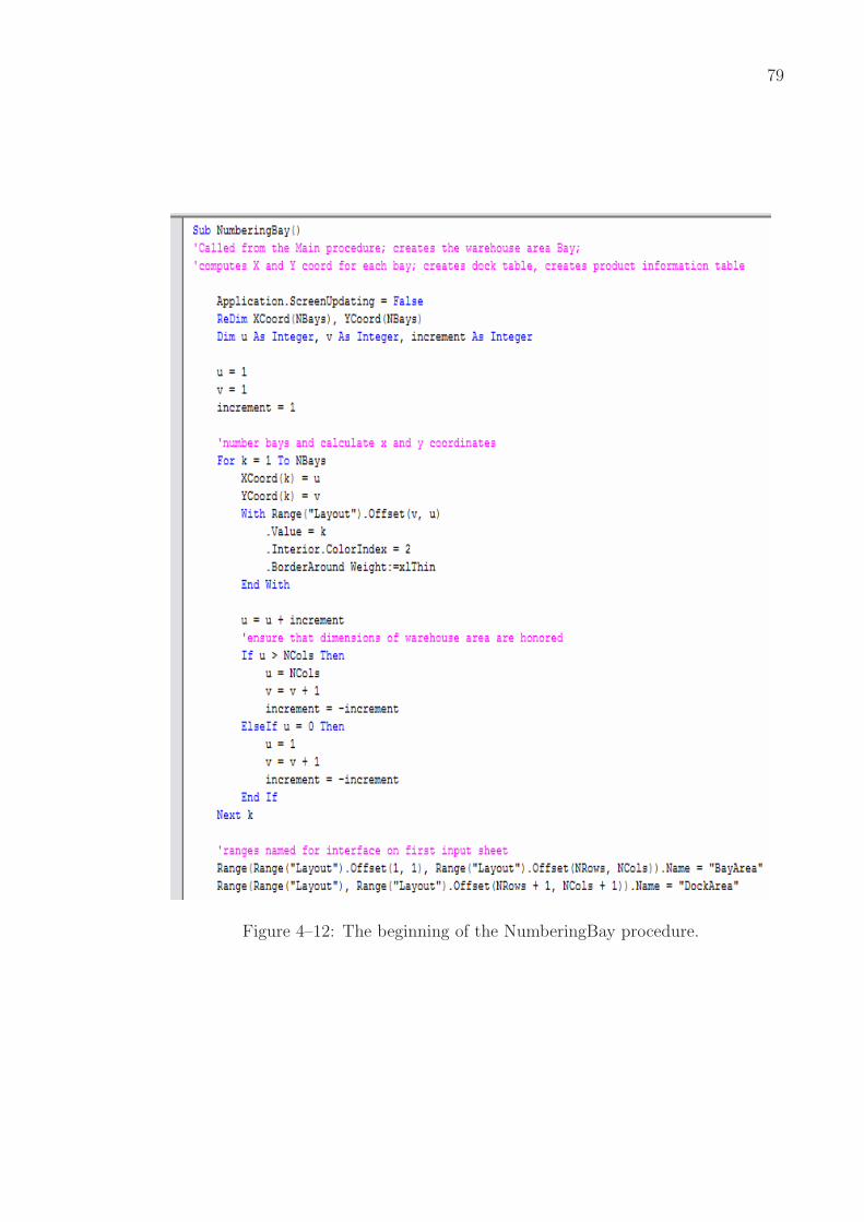
79

Figure 4–12: The beginning of the NumberingBay procedure.

80

Figure 4–13: The end of the NumberingBay procedure.

Knowing that the docks are placed adjacent to the warehouse area and given

the bay numbers to which each dock is adjacent, we can determine the dock

coordinates by determining which border the adjacent bay is on. If the adjacent

bay is on the top or bottom border of the warehouse area (that is, on the first or

last row), then the X coordinate should be zero or one more than the number of

rows, respectively. The Y coordinate will be the same as the Y coordinate of the

adjacent bay. If the adjacent bay is on the left or right border of the warehouse

area (that is, on the first or last column), then the Y coordinate will be zero or one

more than the number of columns, respectively. The X coordinate will be the same

as that of the adjacent bay.

We also record the dock frequencies into an array. Finally, we take the user to

the second input sheet.

81

Figure 4–14: The SelectionChange event procedure enables the user to click on thesheet to place the docks.

The next procedure performs the main calculations and calls the procedures

which execute the algorithm. This is the FinalSteps procedure (see Figure 4.16).

This procedure is assigned to the “Solve” button on the second input sheet. The

procedure begins with two error checks to ensure that the product type table has

been completely filled and that the sum of the required bays is less than or equal to

the total number of bays in the warehouse.

Next, the ComputeF procedure is called (see Figure 4.17). This procedure

computes the weighted distances using the recorded dock frequencies. These

distance weights are equivalent to the ?k values described in the model. We define

γk =∑n

j=1 dkj ∗ Fj and so compute these values using a loop over each bay with

their respective X and Y coordinates and a sub loop over each dock with their

respective frequency values and X and Y coordinates.

82

Figure 4–15: The DockInfo procedure records the dock information.

83

Figure 4–16: The FinalSteps procedure performs the main calculations and call theprocedures which execute the algorithm.

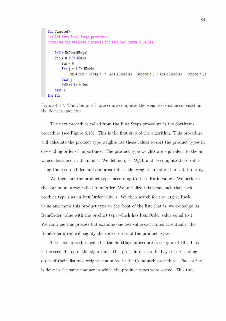
84

Figure 4–17: The ComputeF procedure computes the weighted distances based onthe dock frequencies.

The next procedure called from the FinalSteps procedure is the SortItems

procedure (see Figure 4.18). This is the first step of the algorithm. This procedure

will calculate the product type weights use these values to sort the product types in

descending order of importance. The product type weights are equivalent to the ai

values described in the model. We define αi = Di/Ai and so compute these values

using the recorded demand and area values; the weights are stored in a Ratio array.

We then sort the product types according to these Ratio values. We perform

the sort on an array called ItemOrder. We initialize this array such that each

product type i as an ItemOrder value i. We then search for the largest Ratio

value and move this product type to the front of the list; that is, we exchange its

ItemOrder value with the product type which has ItemOrder value equal to 1.

We continue this process but examine one less value each time. Eventually, the

ItemOrder array will signify the sorted order of the product types.

The next procedure called is the SortBays procedure (see Figure 4.19). This

is the second step of the algorithm. This procedure sorts the bays in descending

order of their distance weights computed in the ComputeF procedure. The sorting

is done in the same manner in which the product types were sorted. This time

85

Figure 4–18: The SortItems procedure calculates the product type weights andsorts them.

86

Figure 4–19: The SortBays algorithm sorts the bays in ascending order of theirdistance weights.

however, we search for the minimum weight value in each pass. We use an array

called BayOrder to store the bay order.

The final procedure called from the FinalSteps procedure is the Assign

procedure (see Figure 4.20). This is the last step of the algorithm. This procedure

completes the assignment of bays to each product type and creates the final layout.

The procedure begins with some formatting for the final layout. There is then

a small section of code which is related to the resolve options; we will discuss this

in more detail in the next section. The assignment loop then begins. We loop

through the sorted list of product types in the descending order of their weight

values found in the SortItems procedure. We then assign bays to each product by

87

looping through the list of sorted bays until the area requirement for the product

type has been met. To reflect that an assignment has been made, we format the

assigned bay with the color of the product type. When the assignment is finished

for the product type, we also update our legend with the product type’s color and

index.

The last part of this procedure simply formats the resulting layout and creates

a “Resolve Layout” which we discuss in the next section. We now return to the

FinalSteps procedure which takes the user to the output sheet.

The only remaining procedures are for the navigational buttons (see 4.22).

These include the “End” button, “View Product Info” button, “View Dock Info”

button, and “Go Back” buttons. Each procedure simply hides and shows the

appropriate sheets.

4.5 Resolve Options

There are two main resolve options for this DSS. The first option allows the

user to revisit the input sheets and change previously entered values. For this

option, the user would use the navigational buttons on the output sheet to return

to either of the input sheets. Suppose, for example, that the user returns to the

first input sheet (see Figure 4.23). Here they may change the location of the docks

or the frequencies of the docks. In Figure 4.23, we have changed the frequencies

from 20% and 80% to 50% and 50% respectively. The user can then press the “Go

Back” button to return to the output sheet.

At this point, the user can press the “Resolve” button to see the new layout

with the changed dock information, or they can choose the other navigational

button to revisit the second input sheet. Let us suppose the user also revisits the

second input sheet to modify the product type information. In Figure 4.24, we have

changed the area requirements for the product types from 2, 4, and 7 to 4, 10, and

88

Figure 4–20: The beginning of the Assign procedure.

89

Figure 4–21: The end of the Assign procedure.

Figure 4–22: The navigational procedures.

90


Main Initializes application, displays input form, callsClearPrevious and NumberingBays, takes user to firstinput sheet.

ClearPrevious Clears values and formatting on all sheet, initializesvariables.

cmdOK Click Does some error checking, assigns input values to corre-sponding variables.

NumberingBays Creates initial layout, determines X and Y coordinatesfor all bays, creates dock and product type tables.

Worksheet Selec-tionChange

Allows user to place docks adjacent to warehouse area,keeps track of number of docks added.

DockInfo Does some error checking, determines X and Y coor-dinates for the docks based on adjacent bays, recordsdock frequencies.

FinalSteps Does some error checking, records product type areasand demands, calls ComputeF, SortItems, SortBays,and Assign, takes user to output sheet.

ComputeF Computes bay distance weights based on dock frequen-cies and bay X and Y coordinates.

SortItems Computes product type weights based on the ratio be-tween their demands and areas, sorts the product typesin descending order of these weights.

SortBays Sorts the bays in ascending order of their distanceweights.

Assign Creates final layout by assigning products to bays intheir sorted orders until all product type area require-ments are satisfied.

Figure 4–23: The first input sheet is revisited and some of the dock information ischanged.

91

Figure 4–24: The second input sheet is revisited and the product type informationis changed.

Figure 4–25: The new layout is displayed after pressing the “Resolve” button.

10 respectively. We have also changed the demand values from 300, 500, and 600

to 500, 600, and 800 respectively. The user can again use the “Go Back” button to

return to the output sheet.

If the user now presses the “Resolve” button, the main procedures will be

rerun and a new layout will be displayed. In Figure 4.25, we show the result of

the resolved layout after making the above changes to the dock and product type

information.

92

Figure 4–26: The resolve options allow the user to specify a particular product’slayout on the Resolve Layout grid.

The second resolve option allows the user to enforce bay assignments for any

of the product types. To do this, the user should select the product type they wish

to enforce from the legend. They can then click on the desired bay assignments

in the “Resolve Layout.” For example, suppose the user wants to enforce the bay

assignments for all of the bays required for product type 2. The user would click

on the “P2” cell in the legend and then click on the desired assignment bays in the

“Resolve Layout” (see Figure 4.26).

The user can then press the “Resolve” button to see the updated layout with

these enforced assignments. In Figure 4.27, we show the modified layout after

enforcing the bay assignments for product type 2. The other assignments are now

made given that product type 2 will be assigned to the specified bays.

Not all of the required bays for any product type need to be enforced. For

example, instead of enforcing all four of the required bays for product 2, the user

could have only enforced the assignment of two of the bays. Multiple product types

can also be enforced at once. In Figure 4.28, we enforce the same bay assignments

for product type 2 as well as six of the seven required bays for product type 3.

93

Figure 4–27: The layout has been resolved with the user’s specifications enforced.

Figure 4–28: Bay assignments for multiple product types can be enforced.

94

Figure 4–29: The final layout is modified to honor the enforced bay assignments.

The resulting layout is shown in Figure 4.29 after the “Resolve” button has

been pressed.

To allow the user to enforce bay assignments with this interface, we have

written a SelectChange event procedure associated with the output sheet (see

Figure 4.30). This procedure is similar to the SelectChange event procedure

associated with the first input sheet in that we have to first check the location of

the selected cell using Union functions.

We first check if the user has clicked in the legend area. If so, then we record

which product type has been selected. Once a product type is selected, the user

may click in the “Resolve Layout” area to specify the enforced assignments. We

check that the next cell clicked is indeed in this layout area and reformat the

selected cell with the product type’s color.

We also record that the selected bay has been fixed; this is recorded in a

Boolean array called FixedBay. We must also ensure that the user does not specify

more bay assignments than the required number of bays for the selected product

95

type. We do this by keeping track of the number of bays which have been assigned

for the selected product type in a FixedProd array.

We can now discuss the Resolve procedure which re-performs the calculations

and re-runs the algorithm for either of these two resolve options (see Figure 4.31).

Since we have stored which bay assignments are fixed, we will skip those bays when

we reach the Assign procedure. Therefore, we begin the procedure by copying the

“Resolve Layout” to capture the assignments made by the user.

We then clear the output sheet and recall the DockInfo and FinalSteps

procedures. These procedures will re-record the information from the dock table

and product type table on the input sheets to capture any changes made by the

user to the input values. The assignment algorithm will then be executed, this

time ignoring the bays which have already been fixed. The resulting layout will

reflect the user’s enforced assignments. We then reset the FixedProd and FixedBay

arrays.


First resolve option Use view buttons to return to input sheets and modifyvalues; then press “Resolve” button to see new layout.

Second resolve op-tion

Enforce some product type bay assignments by click-ing on a product type from the legend and specifyingenforced assignments on “Resolve Layout”; then press“Resolve” button to see new layout.

Worksheet Selec-tionChange

Event procedure to allow user to make assignment en-forcements; it records which bays are fixed and howmany bays have been fixed for each product type.

Resolve Copies the “Resolve Layout” and recalls the DockInfoand FinalSteps procedures; reassigns bays ignoringthose that were fixed by the user.

96

Figure 4–30: The SelectChange event procedure allows the user to enforce particu-lar bay assignments for selected product types.

97

Figure 4–31: The Resolve procedure records changes made to input values andhonors enforced bay assignments.

CHAPTER 5RELIABILITY ANALYSIS


This case study is a DSS application of the reliability analysis problem.

The reliability analysis problem estimates the system failure time of a system of

machines.

5.1.1 Model Definition and Assumptions

In this application, we consider a series parallel system of machines in which

there are three machine types each working in parallel and connected serially (see

Figure 5.1).

To determine failure, we consider each machine type to have a k out of n

system. Given there are n machines in a machine type, any time k of these n

machines fail, the entire machine type fails. We then consider the entire system of

all machine types to also be a k out of n system. In this application, we assume

n = 3 machine types and k = 1. That is, any time one machine type fails, the

entire system fails.

We use the Weibull distribution to estimate the failure times of the machines

in each machine type. Weibull random variables are the most common random

variables used to model failure times of machines (For more details, see Winston

[5]). The cumulative distribution function of the Weibull distribution is as follows.

F (t) = 1− e((−t/β)α) (5.1)

98

99

A1

A2

A3

A4

B1

B2

B3

C1

C2

C3

C4

C5

Figure 5–1: An example of a parallel serial system.

Thus, the inverse function for the Weibull distribution is.

X = β ∗ (ln(1/1− p)α (5.2)

Where p is the probability that X is in the Weibull distribution, and X is the

Weibull random variable. We will use this function to generate random Weibull

values for the simulation. However, we first need to find the parameters α and β.

We optimize the Weibull parameters for each machine type based on their given

means and standard deviations of time to failure. We simulate the system failure

time using these Weibull parameters.

For this application, we analyze the distribution of the system failure time.

We also try to identify which machine type causes the most system failure. We

wish to correct the bottleneck machine type and improve the overall performance

of the system. The output sheet for this analysis includes a histogram of the

system failure time with the mean system failure time as well as a histogram of the

frequency with which a particular machine type caused the system failure.

5.1.2 Input

Using the model described in the above section, we can define the following

input.

100

• Number of machines per machine type (n)

• Number of machine which cause failure per machine type (k)

• Cost per machine for each machine type

• Mean and standard deviation of time to failure for each machine type

• Number of runs to perform in the simulation

We use one user form to receive the first four input values from the user. We

also use one Input Box to record the number of runs to perform. We keep the input

values on a table in the simulation sheet to enable the user to modify them at any

time.

5.1.3 Output

Our output can be defined as follows.

• Optimal Weibull parameters per machine type

• Mean system failure time

• Histogram of system failure times from simulation

• Histogram of frequency with which each machine type caused system failure

from the simulation

The output is shown on the output sheet. There are also some important

resolve options which we discuss in a later section.

5.2 Spreadsheets

We use six spreadsheets in this application: the welcome sheet, a calculation

sheet for optimizing the Weibull parameters, a hidden calculation sheet for prepar-

ing the simulation data, a simulation sheet, another calculation sheet for recording

the results of the simulation runs, and the output sheet. The welcome sheet gives

a description of the application and has a “Start” button assigned to the Main

procedure (see Figure 5.2).

101

Figure 5–2: The welcome sheet.

The first calculation sheet is used to optimize the Weibull parameters for each

machine type (see Figure 5.3). The optimization is performed using the Solver;

therefore, the sheet is organized with ranges for the decision variables, constraints,

and objective function. The input cells for this optimization are the mean and

standard deviation for time to failure for each machine type. Each machine type’s

Weibull parameters are optimized one at a time.

The decision variables are the Weibull parameters alpha and beta. Both of

these have the upper and lower bounds shown adjacent to their cells. These bounds

are the only constraints. We then calculate a mean and standard deviation time to

failure using these alpha and beta to find the square error compared to the user’s

input for these values. The objective function is therefore to minimize the sum of

these square errors.

There are two buttons on this sheet: “End” and “Back.” The “End” button

returns the user to the welcome sheet and the “Back” button is used to return to

the output sheet once the application is completed.

102

Figure 5–3: The calculation sheet for optimizing the Weibull parameters.

We then use a hidden calculation sheet to create a timeline of failure times for

each run of the simulation (see Figure 5.4). The time to failure for each machine on

all machine types is recorded. The machine number and machine type will be used

in the animation.

The next sheet the user sees is the simulation sheet. The simulation sheet

contains an input table and the simulation animation layout (see Figure 5.5). The

input table summarizes all of the input values given by the user in an initial input

form. It also reports the Weibull parameters optimized in the previous sheet. The

user can modify these values at any time and they will be recorded before the

simulation is run.

The animation layout shows all of the machines for each machine type. As

the simulation is run, a failed machine will change to red in the animation. If a

particular machine type reaches its respective k number of failed machines, then a

system failure occurs. The word “Failed” appears above the machine type which

103

Figure 5–4: The hidden calculation sheet for the simulation data.

caused the system failure. In Figure 5.4, machine type A has caused the system

failure since six of its machines have failed; as you can see in the input table, six of

the ten machines are required to cause a failure for machine type A.

There are two buttons plus a hidden button on this sheet. The “End” button

brings the user to the welcome sheet and the “Start Simulation” button calls the

procedure which begins the simulation. The hidden buttons is the “View Analysis”

button which is made visible once the simulation has been completed. It takes the

user to the output sheet.

The next sheet is another calculation sheet which contains the results of each

run of the simulation (see Figure 5.6). The time until the system failed is recorded

along with the machine type which caused the system failure. The table for bin

values is used later in creating the histogram for the machine types.

There are two buttons on this sheet: “End” and “Back.” They have the same

functionalities as the buttons on the first calculation sheet.

The final sheet is the output sheet (see Figures 5.7 and 5.8). This sheet

displays the mean system failure time, a histogram of the system time failures from

104

Figure 5–5: The simulation sheet with the animation layout and input table.

Figure 5–6: The third calculation sheet for the results of the simulation runs.

105

the simulation, and a histogram of the frequencies with which each machine type

caused the system failure. This is the most important information for the user to

analyze to determine how the system is behaving.

There are several buttons on this sheet. The “End” button returns the user

to the welcome sheet. The “View Details” button takes the user to the third

calculation sheet in which the results of the simulation runs are recorded. The

“View Weibull” button takes the user to the first calculation sheet in which the

Weibull parameters were optimized. The last two buttons, “Return to Simulation”

and “Resolve” are used with the resolve options which we discuss in a later section.


Welcome sheet Application description and “Start” button.First calculationsheet

Optimizes the Weibull parameters using the Solver.“End” and “Back” buttons.

Hidden calculationsheet

Creates a timeline of failure times for the simulationanimation.

Simulation sheet Input table and animation layout. “End,” “Start Simu-lation,” and “View Analysis” buttons.

Third calculationsheet

Results of all simulation runs. “End” and “Back” but-tons.

Output sheet Mean system failure time, histogram for system fail-ure times, and histogram for machine type failures.“End,” “View Details,” “View Weibull,” “Return toSimulation” and “Resolve” buttons.

5.3 User Interface

For this application, we have one user form, one input table, several naviga-

tional buttons, and a few functional buttons. We also use one Input Box and one

Message Box. The user form contains input for each machine type (see Figure 5.9).

It prompts the user for the number of machines, number of machines which cause

failure, cost per machine, and the mean and standard deviation of time to failure

for the machine type. We use two frames to group similar text boxes. The “OK”

button has an associated Click procedure which we describe later.

106

Figure 5–7: The top half of the output sheet.

107

Figure 5–8: The bottom half of the output sheet.

This form is shown to the user three times in order to receive the input for

each machine type. We have a dynamic label at the top of the sheet which shows

the name of the current machine type the input will be associated with. Notice

that we use a label and not a text box for this value since the user should never

modify its value.

The input table on the simulation sheet has been described in the previous

section. It simply summarizes the input provided by the user in the user form as

well as the optimized Weibull parameters. The user can change this input before

the simulation is run. The navigational buttons and functional buttons were also

discussed in the previous section with each corresponding worksheet.

The Input Box is used to prompt the user for the number of runs for which the

simulation should be run (see Figure 5.10). A title is given to the Input Box as well

as a default value of 25 runs.

The Message Box is used to inform the reader that the Weibull parameter

optimization has been completed (see Figure 5.11). The corresponding calculation

sheet appears behind the Message Box. We take the user directly to the simulation

sheet not allowing them to pause on the calculation sheet. They can however

108

Figure 5–9: The input form with the dynamic label value for machine type “A.”

Figure 5–10: The Input Box.

109

Figure 5–11: The Message Box.

revisit the Weibull parameter optimization calculations once the simulation is

complete.


Input Form Receives the initial input from the user.Input table on simu-lation sheet

Summarizes the user input and displays the optimizedWeibull parameters for each machine type.

Input Box Prompts the user for the number of runs for the simula-tion.

Message Box Informs the user that the Weibull parameters have beenoptimized.

Navigational But-tons

“End,” “Back,” “View Details,” “View Weibull,” “Re-turn to Simulation”

Functional Buttons “Start,” “Start Simulation,” “Resolve”

5.4 Procedures

We will now outline the procedures for this application. We begin with the

Main sub procedure and variable definitions (see Figure 5.12). The variables shown

defined as public variables are used in multiple procedures. All other variables are

defined within the procedure they are used.

The Main procedure begins by calling the ClearPrev procedure. The ClearPrev

procedure is used to initialize variables and clear previous worksheet values (see

Figure 5.13). The formatting for the animation layout is also cleared.

Next, the Main procedure shows the user the input form. A loop is used to do

this so that the input form can be shown for each machine type. The dynamic label

110

is adjusted before the form is shown to display the name of each machine type.

The form values are recorded into arrays using the same index in the loop. The

Click event procedure of the “OK” command button on the input form performs

some error checking and then assigns the input values to the corresponding array

variables (see Figure 5.14).

The Input Box for the number of runs is then shown. Some error checking is

done to check if the user pressed the ”Cancel” button on the Input Box.

The CalcWeibull procedure is then called. The CalcWeibull procedure uses the

Solver commands to find the optimum Weibull parameters for each machine type

(see Figure 5.15). The Solver is prepared by setting the objective function cells,

decision variable cells, and constraints. Then a loop is used to change the input

cells, which contain the mean and standard deviation of time to failure, for each

machine type. Within this loop the Solver is executed and the decision variable cell

values, the alpha and beta values, are recorded for each machine type.

Once we return to the Main procedure, the Message Box is then displayed

to inform the user that the optimal Weibull parameters have been found for each

machine type. The PrepSim procedure is then called. The PrepSim procedure

rerecords the values from the input table on the simulation sheet and then prepares

the animation layout (see Figure 5.16). The input values are rerecorded so that at

a later time, if the user changes the input values, the simulation and animation will

be updated. This feature becomes more relevant when the PrepSim procedure is

called from the main simulation procedure.

The Main procedure then takes the user to the simulation sheet. On the

simulation sheet, the “Start Simulation” button is used to call the StartSim

procedure; this is the main simulation procedure. The StartSim procedure will

initialize the animation, create the simulation data, and perform the simulation and

111

Figure 5–12: The Main procedure and variable declarations.

112

Figure 5–13: The ClearPrev procedure.

113

Figure 5–14: The cmdOK Click event procedure.

animation (see Figures 5.17 and 5.18). The StartSim procedure begins by calling

the PrepSim procedure as explained above.

It then begins a loop, for the number of runs given by the user, in which data

is created, the animation is performed, and the results of the simulation run are

recorded. To create the simulation data, the CreateData procedure is called. The

CreateData procedure generates failure times for each machine in each machine

type (see Figure 5.19). These values are generated using the WeibullInv function

procedure (see Figure 5.20). This function procedure uses the inverse function

given in the model description to produce a random Weibull variable value using

a random probability value from the Rnd() function. The failure times are stored

in the hidden calculation sheet with their corresponding machine number and

machine type name. The values are then sorted based on the failure time to form

the timeline that will be used to perform the animation.

114

Figure 5–15: The CalcWeibull procedure.

115

Figure 5–16: The PrepSim procedure.

116

Figure 5–17: The beginning of the StartSim procedure.

The StartSim procedure can then begin the animation process. It reads

through the time values in the timeline just created and checks which machine

number of which machine type has just failed. It then changes the formatting of

the respective cell on the animation layout to reflect to the user that a machine has

failed. It also checks whether or not enough machines of a particular machine type

have failed to cause system failure. If so, then the word “Failed” is written over the

appropriate machine type column in the animation layout. The time of the system

failure is recorded to the third calculation sheet along with the machine type which

caused the failure.

The animation is paused after each system failure using the Application.Wait

function. The AnalysisPrep procedure is then called.

The AnalysisPrep procedure uses the results recorded for each run on the third

calculation sheet to create the histograms for the system failure and machine type

failures (see Figure 5.20). The mean system failure time is also reported.

117

Figure 5–18: The end of the StartSim procedure.

118

Figure 5–19: The CreateData procedure and WeibullInv function.

119

Figure 5–20: The AnalysisPrep procedure.

The StartSim procedure then displays the ”View Analysis” button on the

simulation sheet.

The only other procedures are the navigational procedures (see Figure

5.21). These are for the “End,” “Back,” “View Analysis,” “View Details,” “View

Weibull,” and “Return to Simulation” buttons.

120

Figure 5–21: The navigational procedures.


Main Initializes application and retrieves initial input fromuser.

ClearPrev Initializes variables, clears previous values, and clearsanimation layout formatting.

cmdOK Click Error checking, assigns input values to correspondingarray variables.

CalcWeibull Envokes Solver to find optimal Weibull parameters foreach machine type.

StartSim Runs the simulation and performs the animation.PrepSim Rerecords input to capture any changes made by the

user, prepares the animation layout.CreateData Creates a timeline of machine failures for all machines

in each machine type.WeibullInv Generates Weibull random variable values.PrepAnalysis Creates histograms and displays mean system failure

time. Navigational For navigational buttons.

121

Figure 5–22: An example of the first resolve option.

5.5 Resolve Options

There are two main resolve options for this DSS. The first option allows the

user to return to the simulation sheet and modify the input table to rerun the

simulation. This is done by pressing the “Return to Simulation” button on the

output sheet.

For example, in Figure 5.22, we have returned to the simulation sheet after

the initial simulation was run. We have changed the values for the “Number of

Machines to Cause Failure” in the input table from 6 for each machine type to

3, 6, and 9. We then press the “Start Simulation” button again to restart the

simulation. We can see that the new input has been recorded as the first machine

type has caused the system failure when 3 of its machines failed.

122

Figure 5–23: Updated analysis from the first resolve option.

We can then view the output sheet again by pressing the “View Analysis”

button to see that indeed the first machine type has caused the majority of the

system failures (see Figure 5.23).

The second resolve option enables the user to determine the system bottleneck

machine type and add one machine to this machine type to improve system

performance; that is, to increase the mean system failure time. This option is

performed by a Resolve procedure that is called when the “Resolve” button on the

output sheet is pressed (see Figure 5.24).

The Resolve procedure will show the user a resolve form in which they can

choose which machine type to add a machine to. However, before doing that, we

want to suggest to the user which machine type would be the best choice. To do

that, the Resolve procedure begins by performing some trials to determine this best

choice. For each machine type, one machine is added and the simulation is rerun.

We then record the improvement in the mean system failure time. After that is

done for all three machine types, we compute a ratio of these improvements to the

machine cost for each machine type. The best choice will be the machine type with

123

the highest ratio; that is, it is most beneficial to add a machine which will cause

the most improvement in system failure time at the least cost.

The resolve form is then shown (see Figure 5.25). When the form is initialized,

we display the improvements in system failure time, machine costs, and ratio

values for each machine on a table in the form (see Figure 5.26). We also update a

dynamic label to display the best choice that we suggest to the user and select the

corresponding option button.

A frame with these option buttons is used to retrieve the user’s selection of

which machine type they want to add a machine to. The ”OK” button will record

this selection and increase the number of machines for this machine type by one

(see Figure 5.27). It will then update the input table and animation layout and

recall the StartSim procedure.

The user can then observe the new simulation and animation. For example, in

Figure 5.28, we have added one machine to the first machine type. Notice that this

modification is reflected in the input table and the animation layout. The user can

then review the analysis to see if the mean system time has indeed improved. This

process may be repeated as many times as the user desires.


First resolve option User presses the “Return to Simulation” button onoutput sheet to return to simulation sheet; they canmodify the input table and rerun the simulation; theanalysis is updated with the new simulation results.

Second resolve op-tion

User presses the “Resolve” button on the output sheetto view the resolve form; the resolve form enables themto add one machine to one machine type; the bestchoice is suggested to the reader after running trialsimulations in the Resolve procedure.

124

Figure 5–24: The Resolve procedure.

125

Figure 5–25: The resolve form.

Figure 5–26: The initialization event procedure for the resolve form.

126

Figure 5–27: The Click event procedure for the ”OK” button on the resolve form.

127

Figure 5–28: An example of the second resolve option.

CHAPTER 6CONCLUSION

6.1 The Importance of DSS


intended to support managerial decision making. A DSS is not meant to replace a

decision maker, but to extend his/her decision making capabilities. It uses data,

provides a clear user interface, and can incorporate the decision maker’s own

insights.

OR graduates are frequently being employed in positions that require devel-

oping DSS which are gaining widespread popularity. Imparting DSS development

skills, which combine OR skills with IT skills, will make graduates highly sought

after in the modern workplace.

6.2 Spreadsheet-Based DSS

In the past few years, several platforms have become available which allows

the integration of DSS development and IT skills into the OR curriculum. For

spreadsheet-based DSS, we recommend using Excel since it is the most widely used

spreadsheet package among managers and engineers, allows data storage and model

building. Excel also has many built-in program as well as many add-on programs

available that wallow optimization and simulation of various models built in Excel.

Excel also has a macro programming language, Visual Basic for Applications

(VBA), which allows building GUIs and manipulating Excel objects. Thus, Excel

provides a platform using which fairly sophisticated DSS applications can be built.

6.3 Developing a DSS

We propose five basic steps for developing a DSS: i) Application Overview:

create a layout of the entire application to understand the flow from the user input

128

129

to the model calculations to the output, ii) Spreadsheets: determine how many

spreadsheets you will need to best handle input, calculations, and output, iii) User

Interface: outline what interface you will need to receive input from the user and

navigate them through the application, iv) Procedures: outline what sub and/or

function procedures you will need in your code to receive the input, perform the

calculations, and display the output, v) DSS Components: decide what resolve

options the user may have. These steps have been our guidelines to developing

decision support systems.

6.4 Conclusion and Future Direction

Using good GUI design and programming principles along with a clear outline

of the purpose and implementation of the application, a DSS can become a very

powerful tool in aiding decision making. We focus here on spreadsheet-based DSS

applications since spreadsheets are commonly used among decision makers in

OR and business. We are making efforts to develop a textbook which can teach

Excel skills, VBA programming, and DSS application development to industrial

engineering, OR, and business students. [6] We feel that this will aid in better

preparing graduates for real life problems.

DSS applications can be further developed to be applied on larger scale real

world problems as well. The case studies we demonstrate here are simplified

versions of such real world problems. Future work includes finding larger scale

applications, related to research or industry topics in OR, and developing advanced

DSS for them. These DSS may use more advanced object-oriented programming

languages such as C ++ or C#, and may also reference other optimization software

such as CPLEX. The development process we propose is still an important factor

in developing a DSS with a friendly user interface and efficient implementation of

models and algorithms so that the decision making process is indeed enhanced.

REFERENCES

[1] D. Power and R. Sharda. “Model-Driven Decision Support Systems: ResearchNeeds and Directions.” (In Press) Management Science.

[2] T. Mandel. Elements of User Interface Design. New York: John Wiley&Sons,1997.

[3] J. Johnson. GUI Bloopers. San Francisco: Morgan Kaufmann, 2000.

[4] R. Francis, L. McGinnis, and J. White. Facilities Layout and Location: AnAnalytical Approach. New York: Prentice Hall, 1998.

[5] W. Winston. Introduction to Probability Models. Belmont: Brooks/Cole,2004.

[6] M. Hanna, R. Ahuja, and W. Winston. Developing Spreadsheet-BasedDecision Support Systems. (In Press) Duxbury Press.

130

BIOGRAPHICAL SKETCH

Michelle Hanna graduated from the University of Florida with a Bachelor

of Science degree in industrial and systems engineering in May 2002. She then

joined the doctoral program there in industrial and systems engineering in August

2002. After taking several doctoral level courses, Michelle decided to switch to

the doctoral program in decision information sciences in the Warrington School

of Business. She is now completing her master’s degree in industrial and systems

engineering.

Michelle is very interested in the development and application of decision

support systems. She has written a textbook in Developing Spreadsheet-Based

Decision Support Systems with coauthors Ravindra K. Ahuja and Wayne L. Win-

ston. She has also given several lectures on this topic at international conferences

and workshops. Michelle plans to continue to use her DSS development skills as

she works on her doctoral research. Her dissertation will be focused on applying

network theory and algorithms to logistics or scheduling problems.

Michelle plans to pursue an academic career in an operations management or

information science department in a business school. She plans to work towards a

tenured position as a professor in either of these areas.

Michelle is the daughter of Dr. Magdi Hanna and Mrs. Roblyn Hanna.

She has one younger brother, Timothy. Her fiance is Onur Seref. She was born

in Georgia, but has lived in Florida for the last 12 years. Her interests include

languages, international cultures, and spirituality.

131

principles of designing and developing spreadsheet

Documents