principal curves: learning, design, and applicationskegl/research/pdfs/keg99.pdf · ·...

PRINCIPAL CURVES: LEARNING, DESIGN, AND APPLICATIONS

BALAZS KEGL

A THESIS

IN

THE DEPARTMENT

OF

COMPUTER SCIENCE

PRESENTED IN PARTIAL FULFILLMENT OF THE REQUIREMENTS

FOR THE DEGREE OF DOCTOR OF PHILOSOPHY

CONCORDIA UNIVERSITY

MONTREAL, QUEBEC, CANADA

DECEMBER 1999

c© BALAZS KEGL, 1999

CONCORDIA UNIVERSITY

School of Graduate Studies

This is to certify that the thesis prepared

By: Mr. Balazs Kegl

Entitled: Principal Curves: Learning, Design, and Applications

and submitted in partial fulfillment of the requirements for the degree of

Doctor of Philosophy (Computer Science)

complies with the regulations of this University and meets the accepted standards with respect to

originality and quality.

Signed by the final examining commitee:

Chair

External Examiner

Examiner

Examiner

Examiner

Supervisor

ApprovedChair of Department or Graduate Program Director

19

Dr. Nabil Esmail, Dean

Faculty of Engineering and Computer Science

To my parents and Agnes

Abstract

Principal Curves: Learning, Design, and Applications

Balazs Kegl, Ph.D.

Concordia University, 2005

The subjects of this thesis are unsupervised learning in general, and principal curves in particu-

lar. Principal curves were originally defined by Hastie [Has84] and Hastie and Stuetzle [HS89]

(hereafter HS) to formally capture the notion of a smooth curve passing through the “middle” of a

d-dimensional probability distribution or data cloud. Based on the definition, HS also developed an

algorithm for constructing principal curves of distributions and data sets.

The field has been very active since Hastie and Stuetzle’s groundbreaking work. Numerous al-

ternative definitions and methods for estimating principal curves have been proposed, and principal

curves were further analyzed and compared with other unsupervised learning techniques. Several

applications in various areas including image analysis, feature extraction, and speech processing

demonstrated that principal curves are not only of theoretical interest, but they also have a legiti-

mate place in the family of practical unsupervised learning techniques.

Although the concept of principal curves as considered by HS has several appealing charac-

teristics, complete theoretical analysis of the model seems to be rather hard. This motivated us

to redefine principal curves in a manner that allowed us to carry out extensive theoretical analysis

while preserving the informal notion of principal curves. Our first contribution to the area is, hence,

a new theoretical model that is analyzed by using tools of statistical learning theory. Our main result

here is the first known consistency proof of a principal curve estimation scheme.

The theoretical model proved to be too restrictive to be practical. However, it inspired the

design of a new practical algorithm to estimate principal curves based on data. The polygonal

line algorithm, which compares favorably with previous methods both in terms of performance and

computational complexity, is our second contribution to the area of principal curves. To complete

the picture, in the last part of the thesis we consider an application of the polygonal line algorithm

to hand-written character skeletonization.

iv

Acknowledgments

I would like to express my deep gratitude to my advisor, Adam Krzyzak, for his help, trust and

invaluable professional support. He suggested the problem, and guided me through the stages of

this research. My great appreciation goes to Tamas Linder for leading me through the initial phases

of this project, for the fruitful discussions on both the theoretical and the algorithmic issues, and for

his constant support in pursuing my ideas. I would also like to thank Tony Kasvand for showing me

the initial directions in the skeletonization project.

v

Contents

List of Figures ix

List of Tables xi

1 Introduction 1

1.1 Unsupervised Learning . . . . . . . . . . . . . . . . . . . . . . . . . . . . . . . . 1

1.1.1 The Formal Model . . . . . . . . . . . . . . . . . . . . . . . . . . . . . . 4

1.1.2 Areas Of Applications . . . . . . . . . . . . . . . . . . . . . . . . . . . . 4

1.1.3 The Simplest Case . . . . . . . . . . . . . . . . . . . . . . . . . . . . . . 5

1.1.4 A More Realistic Model . . . . . . . . . . . . . . . . . . . . . . . . . . . 8

1.2 Principal Curves . . . . . . . . . . . . . . . . . . . . . . . . . . . . . . . . . . . . 9

1.3 Outline of the Thesis . . . . . . . . . . . . . . . . . . . . . . . . . . . . . . . . . 10

2 Vector Quantization and Principal Component Analysis 12

2.1 Vector Quantization . . . . . . . . . . . . . . . . . . . . . . . . . . . . . . . . . . 12

2.1.1 Optimal Vector Quantizer . . . . . . . . . . . . . . . . . . . . . . . . . . 13

2.1.2 Consistency and Rate Of Convergence . . . . . . . . . . . . . . . . . . . . 14

2.1.3 Locally Optimal Vector Quantizer . . . . . . . . . . . . . . . . . . . . . . 15

2.1.4 Generalized Lloyd Algorithm . . . . . . . . . . . . . . . . . . . . . . . . 16

2.2 Principal Component Analysis . . . . . . . . . . . . . . . . . . . . . . . . . . . . 17

2.2.1 One-Dimensional Curves . . . . . . . . . . . . . . . . . . . . . . . . . . . 18

2.2.2 Principal Component Analysis . . . . . . . . . . . . . . . . . . . . . . . . 22

2.2.3 Properties of the First Principal Component Line . . . . . . . . . . . . . . 25

2.2.4 A Fast PCA Algorithm for Data Sets . . . . . . . . . . . . . . . . . . . . . 26

3 Principal Curves and Related Areas 28

3.1 Principal Curves with Self-Consistency Property . . . . . . . . . . . . . . . . . . 28

3.1.1 The HS Definition . . . . . . . . . . . . . . . . . . . . . . . . . . . . . . 28

vi

3.1.2 The HS Algorithm for Data Sets . . . . . . . . . . . . . . . . . . . . . . . 31

3.1.3 The Bias of the HS Algorithm . . . . . . . . . . . . . . . . . . . . . . . . 33

3.2 Alternative Definitions and Related Concepts . . . . . . . . . . . . . . . . . . . . 36

3.2.1 Alternative Definitions of Principal Curves . . . . . . . . . . . . . . . . . 36

3.2.2 The Self-Organizing Map . . . . . . . . . . . . . . . . . . . . . . . . . . 37

3.2.3 Nonlinear Principal Component Analysis . . . . . . . . . . . . . . . . . . 42

4 Learning Principal Curves with a Length Constraint 44

4.1 Principal Curves with a Length Constraint . . . . . . . . . . . . . . . . . . . . . . 44

4.2 Learning Principal Curves . . . . . . . . . . . . . . . . . . . . . . . . . . . . . . 47

5 The Polygonal Line Algorithm 56

5.1 The Polygonal Line Algorithm . . . . . . . . . . . . . . . . . . . . . . . . . . . . 56

5.1.1 Stopping Condition . . . . . . . . . . . . . . . . . . . . . . . . . . . . . . 58

5.1.2 The Curvature Penalty . . . . . . . . . . . . . . . . . . . . . . . . . . . . 59

5.1.3 The Penalty Factor . . . . . . . . . . . . . . . . . . . . . . . . . . . . . . 60

5.1.4 The Projection Step . . . . . . . . . . . . . . . . . . . . . . . . . . . . . . 61

5.1.5 The Vertex Optimization Step . . . . . . . . . . . . . . . . . . . . . . . . 61

5.1.6 Convergence of the Inner Loop . . . . . . . . . . . . . . . . . . . . . . . . 63

5.1.7 Adding a New Vertex . . . . . . . . . . . . . . . . . . . . . . . . . . . . . 64

5.1.8 Computational Complexity . . . . . . . . . . . . . . . . . . . . . . . . . . 65

5.1.9 Remarks . . . . . . . . . . . . . . . . . . . . . . . . . . . . . . . . . . . 67

5.2 Experimental Results . . . . . . . . . . . . . . . . . . . . . . . . . . . . . . . . . 68

5.2.1 Comparative Experiments . . . . . . . . . . . . . . . . . . . . . . . . . . 69

5.2.2 Quantitative Analysis . . . . . . . . . . . . . . . . . . . . . . . . . . . . . 71

5.2.3 Failure Modes . . . . . . . . . . . . . . . . . . . . . . . . . . . . . . . . 77

6 Application of Principal Curves to Hand-Written Character Skeletonization 82

6.1 Related Work . . . . . . . . . . . . . . . . . . . . . . . . . . . . . . . . . . . . . 83

6.1.1 Applications and Extensions of the HS Algorithm . . . . . . . . . . . . . . 83

6.1.2 Piecewise Linear Approach to Skeletonization . . . . . . . . . . . . . . . 85

6.2 The Principal Graph Algorithm . . . . . . . . . . . . . . . . . . . . . . . . . . . . 85

6.2.1 Principal Graphs . . . . . . . . . . . . . . . . . . . . . . . . . . . . . . . 86

6.2.2 The Initialization Step . . . . . . . . . . . . . . . . . . . . . . . . . . . . 92

6.2.3 The Restructuring Step . . . . . . . . . . . . . . . . . . . . . . . . . . . . 94

6.3 Experimental Results . . . . . . . . . . . . . . . . . . . . . . . . . . . . . . . . . 100

6.3.1 Skeletonizing Isolated Digits . . . . . . . . . . . . . . . . . . . . . . . . . 100

vii

6.3.2 Skeletonizing and Compressing Continuous Handwriting . . . . . . . . . . 105

7 Conclusion 109

Bibliography 111

viii

List of Figures

1 An ill-defined unsupervised learning problem . . . . . . . . . . . . . . . . . . . . 2

2 Projecting points to a curve . . . . . . . . . . . . . . . . . . . . . . . . . . . . . . 19

3 Geometrical properties of curves . . . . . . . . . . . . . . . . . . . . . . . . . . . 20

4 Distance of a point and a line segment . . . . . . . . . . . . . . . . . . . . . . . . 22

5 The first principal component line . . . . . . . . . . . . . . . . . . . . . . . . . . 25

6 Self-consistency . . . . . . . . . . . . . . . . . . . . . . . . . . . . . . . . . . . . 29

7 Computing projection points . . . . . . . . . . . . . . . . . . . . . . . . . . . . . 32

8 The two sources of bias of the HS algorithm . . . . . . . . . . . . . . . . . . . . . 35

9 The flow chart of the polygonal line algorithm . . . . . . . . . . . . . . . . . . . . 57

10 The evolution of the polygonal principal curve . . . . . . . . . . . . . . . . . . . . 58

11 A nearest neighbor partition of induced by the vertices and segments of f . . . . . . 62

12 The flow chart of the optimization step . . . . . . . . . . . . . . . . . . . . . . . . 64

13 ∆′n(f) may be less than ∆n(f) . . . . . . . . . . . . . . . . . . . . . . . . . . . . . 64

14 The circle example . . . . . . . . . . . . . . . . . . . . . . . . . . . . . . . . . . 70

15 The half circle example . . . . . . . . . . . . . . . . . . . . . . . . . . . . . . . . 71

16 Transformed data sets . . . . . . . . . . . . . . . . . . . . . . . . . . . . . . . . . 72

17 Small noise variance . . . . . . . . . . . . . . . . . . . . . . . . . . . . . . . . . 73

18 Large sample size . . . . . . . . . . . . . . . . . . . . . . . . . . . . . . . . . . . 74

19 Sample runs for the quantitative analysis . . . . . . . . . . . . . . . . . . . . . . . 75

20 The average distance of the generating curve and the polygonal principal curve. . . 76

21 The relative difference between the standard deviation of the noise and the measured

RMSE. . . . . . . . . . . . . . . . . . . . . . . . . . . . . . . . . . . . . . . . . . 76

22 Failure modes 1: zig-zagging curves . . . . . . . . . . . . . . . . . . . . . . . . . 77

23 Correction 1: decrease the penalty parameter . . . . . . . . . . . . . . . . . . . . 78

24 Failure modes 2: complex generating curves . . . . . . . . . . . . . . . . . . . . . 80

25 Correction 2: “smart” initialization . . . . . . . . . . . . . . . . . . . . . . . . . . 81

26 Representing a binary image by the integer coordinates of its black pixels . . . . . 86

ix

27 Results on characters not containing loops or crossings . . . . . . . . . . . . . . . 87

28 The flow chart of the extended polygonal line algorithm . . . . . . . . . . . . . . . 88

29 Evolution of the skeleton graph . . . . . . . . . . . . . . . . . . . . . . . . . . . . 89

30 Roles of vertices of different types . . . . . . . . . . . . . . . . . . . . . . . . . . 90

31 Examples of transforming the skeleton into an initial skeleton graph . . . . . . . . 95

32 Paths, loops, simple paths, branches, and deletion . . . . . . . . . . . . . . . . . . 96

33 The role of the angle in deleting short branches . . . . . . . . . . . . . . . . . . . 97

34 Deleting short branches . . . . . . . . . . . . . . . . . . . . . . . . . . . . . . . . 98

35 Removing short loops . . . . . . . . . . . . . . . . . . . . . . . . . . . . . . . . . 99

36 Removing a path in merging star3-vertices . . . . . . . . . . . . . . . . . . . . . . 100

37 Merging star3-vertices . . . . . . . . . . . . . . . . . . . . . . . . . . . . . . . . 101

38 Removing a line-vertex in the filtering operation . . . . . . . . . . . . . . . . . . . 101

39 Filtering vertices . . . . . . . . . . . . . . . . . . . . . . . . . . . . . . . . . . . 102

40 Skeleton graphs of isolated 0’s . . . . . . . . . . . . . . . . . . . . . . . . . . . . 102










50 Original images of continuous handwritings . . . . . . . . . . . . . . . . . . . . . 105

51 Skeleton graphs of continuous handwritings . . . . . . . . . . . . . . . . . . . . . 106

x

List of Tables

1 The relationship between four unsupervised learning algorithms . . . . . . . . . . 68

2 The average radius and RMSE values . . . . . . . . . . . . . . . . . . . . . . . . 75

3 Vertex types and their attributes . . . . . . . . . . . . . . . . . . . . . . . . . . . . 92

4 Vertex degradation rules . . . . . . . . . . . . . . . . . . . . . . . . . . . . . . . 93

5 Length thresholds in experiments with isolated digits . . . . . . . . . . . . . . . . 100

6 Length thresholds in experiments with continuous handwriting . . . . . . . . . . . 105

7 Compression of Alice’s handwriting . . . . . . . . . . . . . . . . . . . . . . . . . 107

8 Compression of Bob’s handwriting . . . . . . . . . . . . . . . . . . . . . . . . . . 108

xi

Chapter 1

Introduction

The subjects of this thesis are unsupervised learning in general, and principal curves in particular. It

is not intended to be a general survey of unsupervised learning techniques, rather a biased overview

of a carefully selected collection of models and methods from the point of view of principal curves.

It can also be considered as a case study of bringing a new baby into the family of unsupervised

learning techniques, describing her genetic relationship with her ancestors and siblings, and indi-

cating her potential prospects in the future by characterizing her talents and weaknesses. We start

the introduction by portraying the family.

1.1 Unsupervised Learning

It is a common practice in general discussions on machine learning to use the dichotomy of super-

vised and unsupervised learning to categorize learning methods. From a conceptual point of view,

supervised learning is substantially simpler than unsupervised learning. In supervised learning, the

task is to guess the value of a random variable Y based on the knowledge of a d-dimensional ran-

dom vector X. The vector X is usually a collection of numerical observations such as a sequence

of bits representing the pixels of an image, and Y represents an unknown nature of the observation

such as the numerical digit depicted by the image. If Y is discrete, the problem of guessing Y is

called classification. Predicting Y means finding a function f : Rd → R such that f (X) is close to Y

where “closeness” is measured by a non-negative cost function q( f (X),Y ). The task is then to find

a function that minimizes the expected cost, that is,

f ∗ = argminf

E[q( f (X),Y )].

In practice, the joint distribution of X and Y is usually unknown, so finding f ∗ analytically is impos-

sible. Instead, we are given Xn = {(X1,Y1), . . . ,(Xn,Yn)} ⊂ Rd ×R, a sample of n independent and

1

identical copies of the pair (X,Y ), and the task is to find a function fn(X) = f (X,Xn) that predicts

Y as well as possible based on the data set Xn. The problem is well-defined in the sense that the

performance of a predictor fn can be quantified by its test error, the average cost measured on an

independent test set X ′m = {(X′

1,Y′1), . . . ,(X

′m,Y ′

m)} defined by

q( f ) =1m

m

∑i=1

q( f (X′i),Y

′i ).

As a consequence, the best of two given predictors f1 and f2 can be chosen objectively by comparing

q( f1) and q( f2) on a sufficiently large test sample.

Unfortunately, this is not the case in unsupervised learning. In a certain sense, an unsupervised

learner can be considered as a supervised learner where the label Y of the observation X is the

observation itself. In other words, the task is to find a function f : Rd → R

d such that f (X) predicts

X as well as possible. Of course, without restricting the set of admissible predictors, this is a trivial

problem. The source of such restrictions is the other objective of unsupervised learning, namely,

to represent the mapping f (X) of X with as few parameters as possible. These two competing

objectives of unsupervised learning are called information preservation and dimension reduction.

The trade-off between the two competing objectives depends on the particular problem. What makes

unsupervised learning ill-defined in certain applications is that the trade-off is often not specified in

the sense that it is possible to find two admissible functions f1 and f2 such that f1 predicts X better

than f2, f2 compresses X more efficiently than f1, and there is no objective criteria to decide which

function performs better overall.

(a) (b)

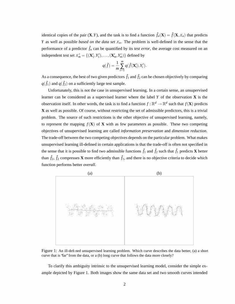
Figure 1: An ill-defined unsupervised learning problem. Which curve describes the data better, (a) a shortcurve that is “far” from the data, or a (b) long curve that follows the data more closely?

To clarify this ambiguity intrinsic to the unsupervised learning model, consider the simple ex-

ample depicted by Figure 1. Both images show the same data set and two smooth curves intended

2

to represent the data set in a concise manner. Using the terminology introduced above, f is a func-

tion that maps every point in the plane to its projection point on the representing curve. Hence, in

this case, the first objective of unsupervised learning means that the representing curve should go

through the data cloud as close to the data points, on average, as possible. Obviously, if this is the

only objective, then the solution is a “snake” that visits all the data points. For restricting the set

of admissible curves, several regularity conditions can be considered. For instance, one can require

that the curve be as smooth as possible, or one can enforce a length limit on the representing curve.

If the length limit is hard, i.e., the length of the curve must be less or equal to a predefined threshold,

the problem is well-defined in the sense that the curve that minimizes the average distance from the

data cloud exists. In practice, however, it is hard to prescribe such a hard limit. Instead, the length

constraint is specified as a soft limit, and the informal objective can be formulated as “find a curve

which is as short as possible and which goes through the data as close to the data points, on average,

as possible”. This “soft” objective clearly makes the problem ill-defined in the sense that without

another principle that decides the actual mixing proportion of the two competing objectives, one

cannot choose the best of two given representing curve. In our example, we need an outside source

that decides between a shorter curve that is farther form the data (Figure 1(a)), or a longer curve that

follows the data more closely (Figure 1(b)).

The reason of placing this discussion even before the formal statement of the problem is that it

determines our philosophy in developing general purpose unsupervised methods. Since the general

problem of unsupervised learning is ill-defined, “turnkey” algorithms cannot be designed. Every

unsupervised learning algorithm must come with a set of parameters that can be used to adjust the

algorithm to a particular problem or according to a particular principle. From the point of view of

the engineer who uses the algorithm, the number of such parameters should be as small as possible,

and their effect on the behavior of the algorithm should be as clear as possible.

The intrinsic ambiguity of the unsupervised learning model also limits the possibilities of the

theoretical analysis. On the one hand, without imposing some restrictive conditions on the model, it

is hard to obtain any meaningful theoretical results. On the other hand, to allow theoretical analysis,

these conditions may be so that the model does not exactly refer to any specific practical problem.

Nevertheless, it is useful to obtain such results to deepen our insight to the model and also to inspire

the development of theoretically well founded practical methods.

In the rest of the section we describe the formal model of unsupervised learning, outline some

of the application areas, and briefly review the possible areas of theoretical analysis.

3

1.1.1 The Formal Model

For the formal description of the problem of unsupervised learning, let D be the domain of the data

and let F be the set of functions of the form f : D → Rd . For each f ∈ F we call the range of f the

manifold generated by f , i.e.,

M f = f (D) = { f (x) : x ∈ D}.

The set of all manifolds generated by all functions in F is denoted by M, i.e., we define

M = {M f : f ∈ F }.

To measure the distortion caused by the mapping of x∈D into M f by the function f , we assume that

a distance ∆(M ,x) is defined for every M ∈ M and x ∈ D. Now consider a random vector X ∈ D.

The distance function or the loss of a manifold M is defined as the expected distance between X

and M , that is,

∆(M ) = E[

∆(X,M )]

.

The general objective of unsupervised learning is to find a manifold M such that ∆(M ) is small

and M has a low complexity relative to the complexity of D. The first objective guarantees that the

information stored in X is preserved by the projection whereas the second objective means that M

is an efficient representation of X.

1.1.2 Areas Of Applications

The general model of unsupervised learning has been defined, analyzed, and applied in many dif-

ferent areas under different names. Some of the most important application areas are the following.

• Clustering or taxonomy in multivariate data analysis [Har75, JD88]. The task is to find a

usually hierarchical categorization of entities (for example, species of animals or plants) on

the basis of their similarities. It is similar to supervised classification in the sense in that

both methods aim to categorize X into a finite number of classes. The difference is that in a

supervised model, the classes are predefined while here the categories are unknown so they

must be created during the process.

• Feature extraction in pattern recognition [DK82, DGL96]. The objective is to find a relatively

small number of features that represent X well in the sense that they preserve most of the vari-

ance of X. Feature extraction is usually used as a pre-processing step before classification to

accelerate the learning by reducing the dimension of the input data. Preserving the informa-

tion stored in X is important to keep the Bayes error (the error that represents the confusion

inherently present in the problem) low.

4

• Lossy data compression in information theory [GG92]. The task is to find an efficient repre-

sentation of X for transmitting it through a communication channel or storing it on a storage

device. The more efficient the compression, the less time is needed for transmission. Keeping

the expected distortion low means that the recovered data at the receiving end resembles the

original.

• Noise reduction in signal processing [VT68]. It is usually assumed here that X was generated

by a latent additive model,

X = M+ ε, (1)

where M is a random vector concentrated to the manifold M , and ε is an independent multi-

variate random noise with zero mean. The task is to recover M based on the noisy observation

X.

• Latent-variable models [Eve84, Mac95, BSW96]. It is presumed that X, although sitting in a

high-dimensional space, has a low intrinsic dimension. This is a special case of (1) when the

additive noise is zero or nearly zero. In practice, M is usually highly nonlinear otherwise the

problem is trivial. When M is two-dimensional, using M for representing X can serve as an

effective visualization tool [Sam69, KW78, BT98].

• Factor analysis [Eve84, Bar87] is another special case of (1) when M is assumed to be a

Gaussian random variable concentrated on a linear subspace of Rd , and ε is a Gaussian noise

with diagonal covariance matrix.

1.1.3 The Simplest Case

In simple unsupervised models the set of admissible functions F or the corresponding set of mani-

folds M is given independently of the distribution of X. F is a set of simple functions in the sense

that any f ∈ F or the corresponding M f ∈ M can be represented by a few parameters. It is also

assumed that any two manifolds in M have the same intrinsic dimension, so the only objective in

this model is to minimize ∆(M ) over M, i.e., to find

M ∗ = argminM ∈M

E[

∆(X,M )]

.

Similarly to supervised learning, the distribution of X is usually unknown in practice. Instead, we

are given Xn = {X1, . . . ,Xn} ⊂ Rd , a sample of n independent and identical copies of X, and the

task is to find a function fn(X) = f (X,Xn) based on the data set Xn that minimizes the distance

function. Since the the distribution of X is unknown, we estimate ∆(M ) by the empirical distance

5

function or empirical loss of M defined by

∆n(M ) =1n

n

∑i=1

∆(Xi,M ). (2)

The problem is well-defined in the sense that the performance of a projection function fn can be

quantified by the empirical loss of fn measured on an independent test set X ′m = {X′

1, . . . ,X′m}. As

a consequence, the best of two given projection functions f1 and f2 can be chosen objectively by

comparing ∆n(M f1) and ∆n(M f2

) on a sufficiently large test sample.

In the theoretical analysis of a particular unsupervised model, the first question to ask is

“Does M ∗ exist in general?” (Q1)

Clearly, if M ∗ does not exist, or it only exists under severe restrictions, the theoretical analysis

of any estimation scheme based on finite data is difficult. If M ∗ does exist, the next two obvious

questions are

“Is M ∗ unique?” (Q2)

and

“Can we show a concrete example of M ∗?” (Q3)

Interestingly, even for some of the simplest unsupervised learning models, the answer to Question 3

is no for even the most common multivariate densities. Note, however, that this fact does not make

the theoretical analysis of an estimating scheme impossible, and does not make it unreasonable to

aim for the optimal loss ∆(M ∗) in practical estimator design.

The most widely used principle in designing nonparametric estimation schemes is the empirical

loss minimization principle. In unsupervised learning this means that based on the data set Xn, we

pick the manifold M ∗n ∈ M that minimizes the empirical distance function (2), i.e., we choose

M ∗n = argmin

M ∈M

1n

n

∑i=1

∆(Xi,M ). (3)

The first property of M ∗n to analyze is its consistency, i.e. the first question is

“Is limn→∞

∆(M ∗n ) = ∆(M ∗) in probability?” (Q4)

Consistency guarantees that by increasing the amount of data, the expected loss of M ∗n gets arbi-

trarily close to the best achievable loss. Once consistency is established, the next natural question

is

“What is the convergence rate of ∆(M ∗n ) → ∆(M ∗)?” (Q5)

6

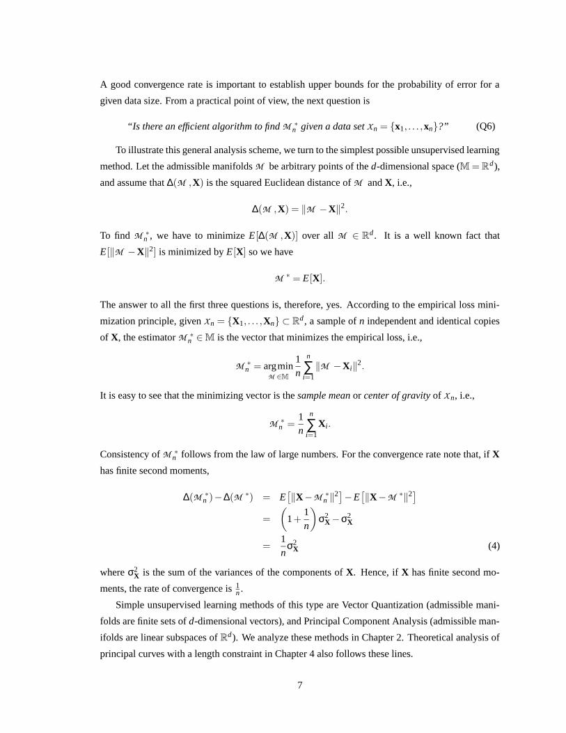
A good convergence rate is important to establish upper bounds for the probability of error for a

given data size. From a practical point of view, the next question is

“Is there an efficient algorithm to find M ∗n given a data set Xn = {x1, . . . ,xn}?” (Q6)

To illustrate this general analysis scheme, we turn to the simplest possible unsupervised learning

method. Let the admissible manifolds M be arbitrary points of the d-dimensional space (M = Rd),

and assume that ∆(M ,X) is the squared Euclidean distance of M and X, i.e.,

∆(M ,X) = ‖M −X‖2.

To find M ∗n , we have to minimize E[∆(M ,X)] over all M ∈ R

d . It is a well known fact that

E[‖M −X‖2] is minimized by E[X] so we have

M ∗ = E[X].

The answer to all the first three questions is, therefore, yes. According to the empirical loss mini-

mization principle, given Xn = {X1, . . . ,Xn} ⊂ Rd , a sample of n independent and identical copies

of X, the estimator M ∗n ∈ M is the vector that minimizes the empirical loss, i.e.,

M ∗n = argmin

M ∈M

1n

n

∑i=1

‖M −Xi‖2.

It is easy to see that the minimizing vector is the sample mean or center of gravity of Xn, i.e.,

M ∗n =

1n

n

∑i=1

Xi.

Consistency of M ∗n follows from the law of large numbers. For the convergence rate note that, if X

has finite second moments,

∆(M ∗n )−∆(M ∗) = E

[

‖X−M ∗n ‖2]−E

[

‖X−M ∗‖2]

=

(

1+1n

)

σ2X −σ2

X

=1n

σ2X (4)

where σ2X is the sum of the variances of the components of X. Hence, if X has finite second mo-

ments, the rate of convergence is 1n .

Simple unsupervised learning methods of this type are Vector Quantization (admissible mani-

folds are finite sets of d-dimensional vectors), and Principal Component Analysis (admissible man-

ifolds are linear subspaces of Rd). We analyze these methods in Chapter 2. Theoretical analysis of

principal curves with a length constraint in Chapter 4 also follows these lines.

7

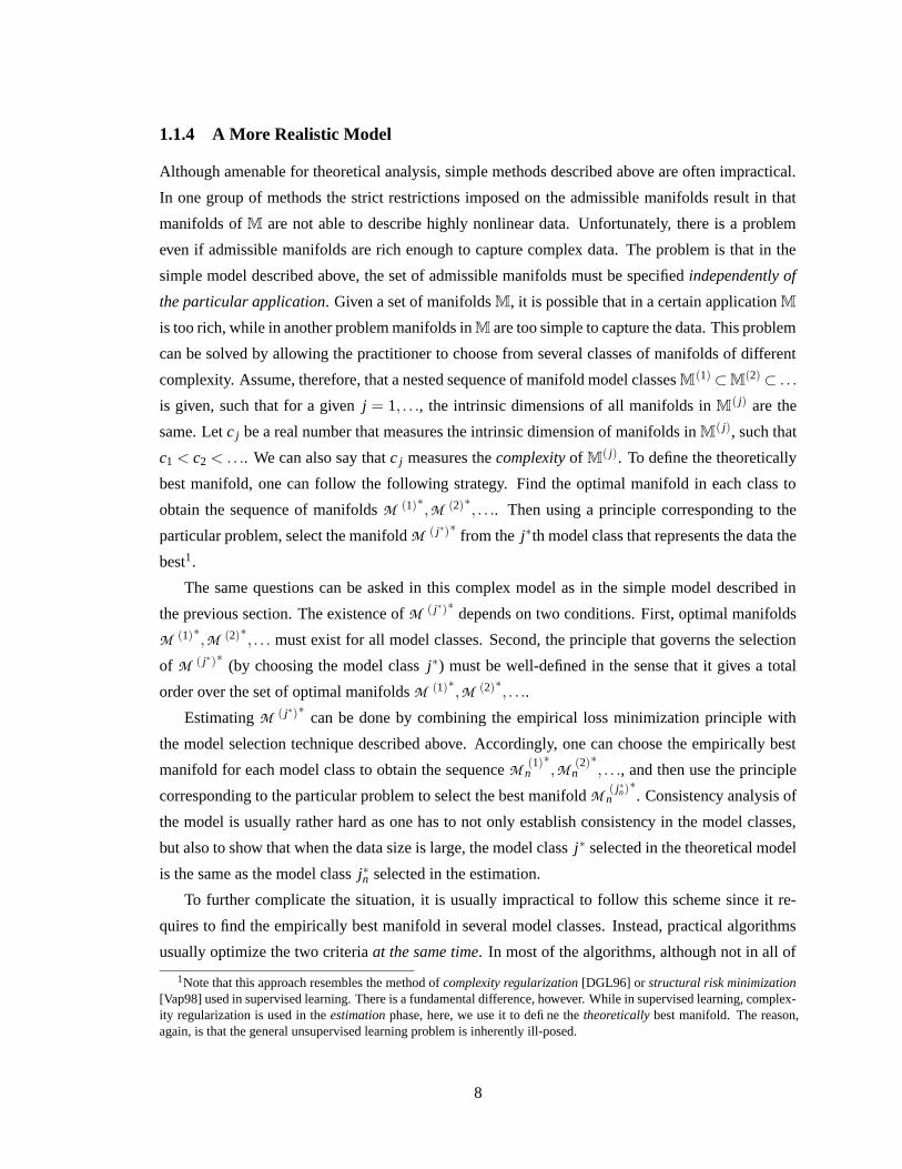
1.1.4 A More Realistic Model

Although amenable for theoretical analysis, simple methods described above are often impractical.

In one group of methods the strict restrictions imposed on the admissible manifolds result in that

manifolds of M are not able to describe highly nonlinear data. Unfortunately, there is a problem

even if admissible manifolds are rich enough to capture complex data. The problem is that in the

simple model described above, the set of admissible manifolds must be specified independently of

the particular application. Given a set of manifolds M, it is possible that in a certain application M

is too rich, while in another problem manifolds in M are too simple to capture the data. This problem

can be solved by allowing the practitioner to choose from several classes of manifolds of different

complexity. Assume, therefore, that a nested sequence of manifold model classes M(1) ⊂M

(2) ⊂ . . .

is given, such that for a given j = 1, . . ., the intrinsic dimensions of all manifolds in M( j) are the

same. Let c j be a real number that measures the intrinsic dimension of manifolds in M( j), such that

c1 < c2 < .. .. We can also say that c j measures the complexity of M( j). To define the theoretically

best manifold, one can follow the following strategy. Find the optimal manifold in each class to

obtain the sequence of manifolds M (1)∗,M (2)∗, . . .. Then using a principle corresponding to the

particular problem, select the manifold M ( j∗)∗ from the j∗th model class that represents the data the

best1.

The same questions can be asked in this complex model as in the simple model described in

the previous section. The existence of M ( j∗)∗ depends on two conditions. First, optimal manifolds

M (1)∗,M (2)∗, . . . must exist for all model classes. Second, the principle that governs the selection

of M ( j∗)∗ (by choosing the model class j∗) must be well-defined in the sense that it gives a total

order over the set of optimal manifolds M (1)∗,M (2)∗, . . ..

Estimating M ( j∗)∗ can be done by combining the empirical loss minimization principle with

the model selection technique described above. Accordingly, one can choose the empirically best

manifold for each model class to obtain the sequence M (1)n

∗,M (2)

n∗, . . ., and then use the principle

corresponding to the particular problem to select the best manifold M ( j∗n)n

∗. Consistency analysis of

the model is usually rather hard as one has to not only establish consistency in the model classes,

but also to show that when the data size is large, the model class j∗ selected in the theoretical model

is the same as the model class j∗n selected in the estimation.

To further complicate the situation, it is usually impractical to follow this scheme since it re-

quires to find the empirically best manifold in several model classes. Instead, practical algorithms

usually optimize the two criteria at the same time. In most of the algorithms, although not in all of

1Note that this approach resembles the method of complexity regularization [DGL96] or structural risk minimization[Vap98] used in supervised learning. There is a fundamental difference, however. While in supervised learning, complex-ity regularization is used in the estimation phase, here, we use it to define the theoretically best manifold. The reason,again, is that the general unsupervised learning problem is inherently ill-posed.

8

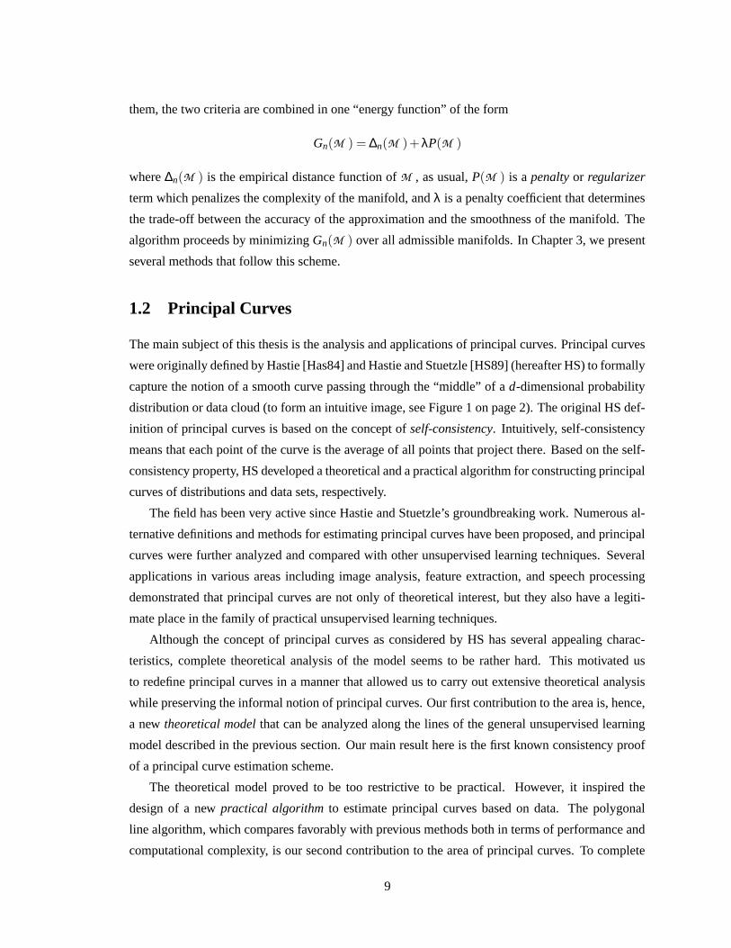
them, the two criteria are combined in one “energy function” of the form

Gn(M ) = ∆n(M )+λP(M )

where ∆n(M ) is the empirical distance function of M , as usual, P(M ) is a penalty or regularizer

term which penalizes the complexity of the manifold, and λ is a penalty coefficient that determines

the trade-off between the accuracy of the approximation and the smoothness of the manifold. The

algorithm proceeds by minimizing Gn(M ) over all admissible manifolds. In Chapter 3, we present

several methods that follow this scheme.

1.2 Principal Curves

The main subject of this thesis is the analysis and applications of principal curves. Principal curves

were originally defined by Hastie [Has84] and Hastie and Stuetzle [HS89] (hereafter HS) to formally

capture the notion of a smooth curve passing through the “middle” of a d-dimensional probability

distribution or data cloud (to form an intuitive image, see Figure 1 on page 2). The original HS def-

inition of principal curves is based on the concept of self-consistency. Intuitively, self-consistency

means that each point of the curve is the average of all points that project there. Based on the self-

consistency property, HS developed a theoretical and a practical algorithm for constructing principal

curves of distributions and data sets, respectively.

The field has been very active since Hastie and Stuetzle’s groundbreaking work. Numerous al-

ternative definitions and methods for estimating principal curves have been proposed, and principal

curves were further analyzed and compared with other unsupervised learning techniques. Several

applications in various areas including image analysis, feature extraction, and speech processing

demonstrated that principal curves are not only of theoretical interest, but they also have a legiti-

mate place in the family of practical unsupervised learning techniques.

Although the concept of principal curves as considered by HS has several appealing charac-

teristics, complete theoretical analysis of the model seems to be rather hard. This motivated us

to redefine principal curves in a manner that allowed us to carry out extensive theoretical analysis

while preserving the informal notion of principal curves. Our first contribution to the area is, hence,

a new theoretical model that can be analyzed along the lines of the general unsupervised learning

model described in the previous section. Our main result here is the first known consistency proof

of a principal curve estimation scheme.

The theoretical model proved to be too restrictive to be practical. However, it inspired the

design of a new practical algorithm to estimate principal curves based on data. The polygonal

line algorithm, which compares favorably with previous methods both in terms of performance and

computational complexity, is our second contribution to the area of principal curves. To complete

9

the picture, in the last part of the thesis we consider an application of the polygonal line algorithm to

hand-written character skeletonization. We note here that parts of our results have been previously

published in [KKLZ], [KKLZ99], and [KKLZ00].

1.3 Outline of the Thesis

Most of the unsupervised learning algorithms originate from one of the two basic unsupervised

learning models, vector quantization and principal component analysis. In Chapter 2 we describe

these two models. In Chapter 3, we present the formal definition of the HS principal curves, describe

the subsequent extensions and analysis, and discuss the relationship between principal curves and

other unsupervised learning techniques.

An unfortunate property of the HS definition is that, in general, it is not known if principal

curves exist for a given distribution. This also makes it difficult to theoretically analyze any esti-

mation scheme for principal curves. In Chapter 4 we propose a new definition of principal curves

and prove the existence of principal curves in the new sense for a large class of distributions. Based

on the new definition, we consider the problem of learning principal curves based on training data.

We introduce and analyze an estimation scheme using a common model in statistical learning the-

ory. The main result of this chapter is a proof of consistency and analysis of rate of convergence

following the general scheme described in Section 1.1.

Although amenable to analysis, our theoretical algorithm is computationally burdensome for

implementation. In Chapter 5 we develop a suboptimal algorithm for learning principal curves. The

polygonal line algorithm produces piecewise linear approximations to the principal curve, just as

the theoretical method does, but global optimization is replaced by a less complex gradient-based

method. We give simulation results and compare our algorithm with previous work. In general,

on examples considered by HS, the performance of the new algorithm is comparable with the HS

algorithm while it proves to be more robust to changes in the data generating model.

Chapter 6 starts with an overview of existing principal curve applications. The main subject of

this chapter is an application of an extended version of the principal curve algorithm to hand-written

character skeletonization. The development of the method was inspired by the apparent similarity

between the definition of principal curves and the medial axis of a character. A principal curve is

a smooth curve that goes through the “middle” of a data set, whereas the medial axis is a set of

smooth curves that go equidistantly from the contours of a character. Since the medial axis can be

a set of connected curves rather then only one curve, in Chapter 6 we extend the polygonal line

algorithm to find a principal graph of a data set. The extended algorithm also contains two elements

specific to the task of skeletonization, an initialization method to capture the approximate topology

of the character, and a collection of restructuring operations to improve the structural quality of the

10

skeleton produced by the initialization method. Test results on isolated hand-written digits indicate

that the algorithm finds a smooth medial axis of the great majority of a wide variety of character

templates. Experiments with images of continuous handwriting demonstrate that the skeleton graph

produced by the algorithm can be used for representing hand-written text efficiently.

11

Chapter 2

Vector Quantization and Principal

Component Analysis

Most of the unsupervised learning algorithms originate from one of the two basic unsupervised

learning models, vector quantization and principal component analysis. In particular, principal

curves are related to both areas: conceptually, they are originated from principal component analysis

whereas practical methods to estimate principal curves often resemble to basic vector quantization

algorithms. This chapter describes these two models.

2.1 Vector Quantization

Vector quantization is an important topic of information theory. Vector quantizers are used in lossy

data compression, speech and image coding [GG92], and clustering [Har75]. Vector quantization

can also be considered as the simplest form of unsupervised learning where the manifold to fit to

the data is a set of vectors. Kohonen’s self-organizing map [Koh97] (introduced in Section 3.2.2)

can also be interpreted as a generalization of vector quantization. Furthermore, our new definition

of principal curves (to be presented in in Section 4.1) has been inspired by the notion of an optimal

vector quantizer. One of the most widely used algorithms for constructing locally optimal vector

quantizers for distributions or data sets is the Generalized Lloyd (GL) algorithm [LBG80] (also

known as the k-means algorithm [Mac67]). Both the HS algorithm (Section 3.1.1) and the polygonal

line algorithm (Section 5.1) are similar in spirit to the GL algorithm. This section introduces the

concept of optimal vector quantization and describes the GL algorithm.

12

2.1.1 Optimal Vector Quantizer

A k-point vector quantizer is a mapping q : Rd →R

d that assigns to each input vector x ∈Rd a code-

point x = q(x) drawn from a finite codebook C = {v1, . . . ,vk} ⊂ Rd . The quantizer is completely

described by the codebook C together with the partition V = {V1, . . . ,Vk} of the input space where

V` = q−1(v`) = {x : q(x) = v`} is the set of input vectors that are mapped to the `th codepoint by q.

The distortion caused by representing an input vector x by a codepoint x is measured by a non-

negative distortion measure ∆(x, x). Many such distortion measures have been proposed in different

areas of application. For the sake of simplicity, in what follows, we assume that ∆(x, x) is the most

widely used squared error distortion, that is,

∆(x, x) = ‖x− x‖2. (5)

The performance of a quantizer q applied to a random vector X = (X1, . . . ,Xd) is measured by

the expected distortion,

∆(q) = E[∆(X,q(X))] (6)

where the expectation is taken with respect to the underlying distribution of X. The quantizer q∗ is

globally optimal if ∆(q∗) ≤ ∆(q) for any k-point quantizer q. It can be shown that q∗ exists if X has

finite second moments, so the answer to Question 1 in Section 1.1.3 is yes. Interestingly, however,

the answers to Questions 2 and 3 are no in general. Finding a globally optimal vector quantizer for

a given source distribution or density is a very hard problem. Presently, for k > 2 codepoints there

seem to be no concrete examples of optimal vector quantizers for even the most common model

distributions such as Gaussian, Laplacian, or uniform (in a hypercube) in any dimensions d > 1.

Since global optimality is not a feasible requirement, algorithms, even in theory, are usually

designed to find locally optimal vector quantizers. A quantizer q is said to be locally optimal if ∆(q)

is only a local minimum, that is, slight disturbance of any of the codepoints will cause an increase

in the distortion. Necessary conditions for local optimality will be given in Section 2.1.3. We also

describe here a theoretical algorithm, the Generalized Lloyd (GL) algorithm [LBG80], to find a

locally optimal vector quantizer of a random variable.

In practice, the distribution of X is usually unknown. Therefore, the objective of empirical

quantizer design is to find a vector quantizer based on Xn = {X1, . . . ,Xn}, a set of independent and

identical copies of X. To design a quantizer with low distortion, most existing practical algorithms

attempt to implement the empirical loss minimization principle introduced for the general unsuper-

vised learning model in Section 1.1.3. The performance of a vector quantizer q on Xn is measured

by the empirical distortion of q given by

∆n(q) =1n

n

∑i=1

∆(Xi,q(Xi)). (7)

13

The quantizer q∗n is globally optimal on the data set Xn if ∆n(q∗n)≤ ∆n(q) for any k-point quantizer q.

Finding an empirically optimal vector quantizer is, in theory, possible since the number of different

partitions of Xn is finite. However, the systematic inspection of all different partitions is computa-

tionally infeasible. Instead, most practical methods use an iterative approach similar in spirit to the

GL algorithm.

It is of both theoretical and practical interest to analyze how the expected loss of the empirically

best vector quantizer ∆(q∗n) relates to the best achievable loss ∆n(q∗), even though q∗ is not known

and q∗n is practically infeasible to obtain. Consistency (Question 4 in Section 1.1.3) of the estimation

scheme means that the expected loss of the q∗n converges in probability to the best achievable loss

as the number of the data points grows, therefore, if we have a perfect algorithm and unlimited

access to data, we can get arbitrarily close to the best achievable loss. A good convergence rate

(Question 5) is important to establish upper bounds for the probability of error for a given data

size. We start the analysis of the empirical loss minimization principle used for vector quantization

design by presenting results on consistency and rate of convergence in Section 2.1.2.

2.1.2 Consistency and Rate Of Convergence

Consistency of the empirical quantizer design under general conditions was proven by Pollard

[Pol81, Pol82]. The first rate of convergence results were obtained by Linder et al. [LLZ94]. In

particular, [LLZ94] showed that if the distribution of X is concentrated on a bounded region, there

exists a constant c such that

∆(q∗n)−∆(q∗) ≤ cd3/2

√

k lognn

. (8)

An extension of this result to distributions with unbounded support is given in [MZ97]. Bartlett et

al. [BLL98] pointed out that the√

logn factor can be eliminated from the upper bound in (8) by

using an analysis based on sophisticated uniform large deviation inequalities of Alexander [Ale84]

or Talagrand [Tal94]. More precisely, it can be proven that there exists a constant c′ such that

∆(q∗n)−∆(q∗) ≤ c′d3/2

√

k log(kd)

n. (9)

There are indications that the upper bound can be tightened to O(1/n). First, in (4) we showed

that if k = 1, the expected loss of the sample average converges to the smallest possible loss at a

rate of O(1/n). Another indication that an O(1/n) rate might be achieved comes from a result of

Pollard [Pol82]. He showed if X has a specially smooth and regular density, the difference between

the codepoints of the empirically designed quantizers and the codepoints of the optimal quantizer

obeys a multidimensional central limit theorem. As Chou [Cho94] pointed out, this implies that that

within the class of distributions considered by [Pol82], the distortion redundancy decreases at a rate

O(1/n). Despite these suggestive facts, it was showed by [BLL98] that in general, the conjectured

14

O(1/n) distortion redundancy rate does not hold. In particular, [BLL98] proved that for any k-point

quantizer qn which is designed by any method from n independent training samples, there exists a

distribution on a bounded subset of Rd such that the expected loss of qn is bounded away from the

optimal distortion by a constant times 1/√

n. Together with (9), this result shows that the minimax

(worst-case) distortion redundancy for empirical quantizer design is asymptotically on the order of

1/√

n. As a final note, [BLL98] conjectures that the minimax expected distortion redundancy is

some constant times

da

√

k1−b/d

n

for some values of a ∈ [1,3/2] and b ∈ [2,4].

2.1.3 Locally Optimal Vector Quantizer

Suppose that we are given a particular codebook C but the partition is not specified. An optimal

partition V can be constructed by mapping each input vector x to the codepoint v` ∈ C that mini-

mizes the distortion ∆(x,v`) among all codepoints, that is, by choosing the nearest codepoint to x.

Formally, V = {V1, . . . ,Vk} is the optimal partition of the codebook C if

V` = {x : ∆(x,v`) ≤ ∆(x,vm), m = 1, . . . ,k}. (10)

(A tie-breaking rule such as choosing the codepoint with the lowest index is required if more than

one codepoint minimizes the distortion.) V` is called the Voronoi region or Voronoi set associated

with the codepoint v`.

Conversely, assume that we are given a partition V = {V1, . . . ,Vk} and an optimal codebook

C = {v1, . . . ,vk} is needed to be constructed. To minimize the expected distortion, we have to set

v` = argminv

E[∆(X,v)|X ∈V`]. (11)

v` is called the centroid or the center of gravity of the set V`, motivated by the fact that for the

squared error distortion (5) we have v` = E[X|X ∈V`].

It can be shown that the nearest neighbor condition (10) and the centroid condition (11) must

hold for any locally optimal vector quantizer. Another necessary condition of local optimality is

that boundary points occur with zero probability, that is,

P{X : X ∈V`,∆(X,v`) = ∆(X,vm), ` 6= m} = 0. (12)

If we have a codebook that satisfies all three necessary conditions of optimality, it is widely be-

lieved that it is indeed locally optimal. No general theoretical derivation of this result has ever been

obtained. For the particular case of discrete distribution, however, it can be shown that under mild

restrictions, a vector quantizer satisfying the three necessary conditions is indeed locally optimal

[GKL80].

15

2.1.4 Generalized Lloyd Algorithm

The nearest neighbor condition and the centroid condition suggest a natural algorithm for designing

a vector quantizer. The GL algorithm alternates between an expectation and a partition step until

the relative improvement of the expected distortion is less than a preset threshold. In the expectation

step the codepoints are computed according to (11), and in the partition step the Voronoi regions are

set by using (10). It is assumed that an initial codebook C (0) is given. When the probability density

of X is known, the GL algorithm for constructing a vector quantizer is the following.

Algorithm 1 (The GL algorithm for distributions)

Step 0 Set j = 0, and set C (0) ={

v(0)1 , . . . ,v(0)

k

}

to an initial codebook.

Step 1 (Partition) Construct V ( j) ={

V ( j)1 , . . . ,V ( j)

k

}

by setting

V ( j)` =

{

x : ∆(

x,v( j)`

)

≤ ∆(

x,v( j)m

)

, m = 1, . . . ,k}

for ` = 1, . . . ,k.

Step 2 (Expectation) Construct C ( j+1) ={

v( j+1)1 , . . . ,v( j+1)

k

}

by setting

v( j+1)` = argminv E

[

∆(X,v)∣

∣

∣X ∈V ( j)

`

]

= E[

X∣

∣

∣X ∈V ( j)

`

]

for ` = 1, . . . ,k.

Step 3 Stop if

(

1− ∆(q( j+1))∆(q( j))

)

is less than or equal to a certain threshold. Otherwise, let j = j +1

and go to Step 1.

Step 1 is complemented with a suitable rule to break ties. When a cell becomes empty in Step 1,

one can split the cell with the highest probability, or the cell with the highest partial distortion into

two, and delete the empty cell.

It is easy to see that ∆(

q( j))

is non-increasing and non-negative, so it must have a limit ∆(

q(∞))

.

[LBG80] showed that if a limiting quantizer C (∞) exists in the sense that C ( j) → C (∞) as j → ∞(in the usual Euclidean sense), then the codepoints of C (∞) are the centroids of the Voronoi regions

induced by C (∞), so C (∞) is a fixed point of the algorithm with zero threshold.

The GL algorithm can easily be adjusted to the case when the distribution of X is unknown but

a set of independent observations Xn = {x1, . . . ,xn} ⊂ Rd of the underlying distribution is known

instead. The modifications are straightforward replacements of the expectations by sample averages.

In Step 3, the empirical distortion

∆n(q) =1n

n

∑i=1

∆(xi,q(xi)) =1n

k

∑=1

∑x∈V`

‖v`−x‖2

is evaluated in place of the unknown expected distortion ∆n(q). The GL algorithm for constructing

a vector quantizer based on the data set Xn is the following.

16

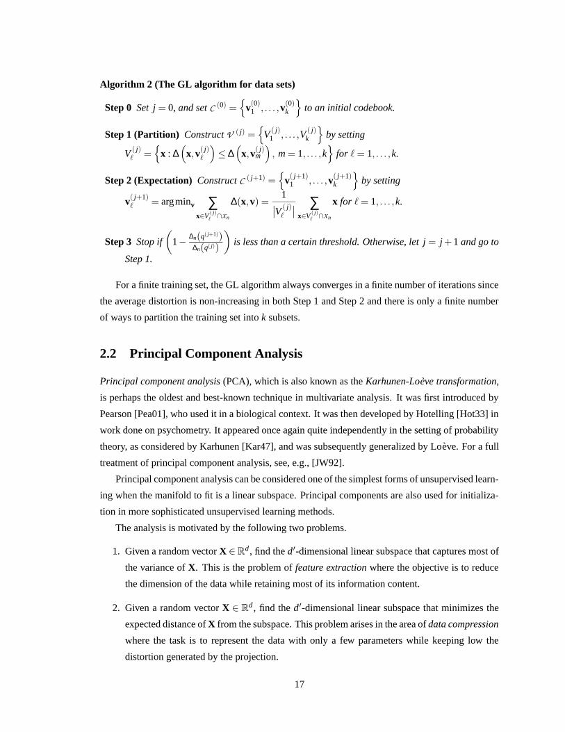
Algorithm 2 (The GL algorithm for data sets)


v(0)1 , . . . ,v(0)

k

}



V ( j)1 , . . . ,V ( j)

k

}

by setting

V ( j)` =

{

x : ∆(

x,v( j)`

)

≤ ∆(

x,v( j)m

)

, m = 1, . . . ,k}

for ` = 1, . . . ,k.


v( j+1)1 , . . . ,v( j+1)

k

}

by setting

v( j+1)` = argminv ∑

x∈V ( j)` ∩Xn

∆(x,v) =1

∣

∣V ( j)`

∣

∣

∑x∈V ( j)

` ∩Xn

x for ` = 1, . . . ,k.

Step 3 Stop if

(

1− ∆n(q( j+1))∆n(q( j))

)

is less than a certain threshold. Otherwise, let j = j +1 and go to

Step 1.

For a finite training set, the GL algorithm always converges in a finite number of iterations since

the average distortion is non-increasing in both Step 1 and Step 2 and there is only a finite number

of ways to partition the training set into k subsets.

2.2 Principal Component Analysis

Principal component analysis (PCA), which is also known as the Karhunen-Loeve transformation,

is perhaps the oldest and best-known technique in multivariate analysis. It was first introduced by

Pearson [Pea01], who used it in a biological context. It was then developed by Hotelling [Hot33] in

work done on psychometry. It appeared once again quite independently in the setting of probability

theory, as considered by Karhunen [Kar47], and was subsequently generalized by Loeve. For a full

treatment of principal component analysis, see, e.g., [JW92].

Principal component analysis can be considered one of the simplest forms of unsupervised learn-

ing when the manifold to fit is a linear subspace. Principal components are also used for initializa-

tion in more sophisticated unsupervised learning methods.

The analysis is motivated by the following two problems.

1. Given a random vector X ∈ Rd , find the d′-dimensional linear subspace that captures most of

the variance of X. This is the problem of feature extraction where the objective is to reduce

the dimension of the data while retaining most of its information content.

2. Given a random vector X ∈ Rd , find the d′-dimensional linear subspace that minimizes the

expected distance of X from the subspace. This problem arises in the area of data compression

where the task is to represent the data with only a few parameters while keeping low the

distortion generated by the projection.

17

It turns out that the two problems have the same solution, and the solution lies in the eigenstructure

of the covariance matrix of X. Before we derive this result in Section 2.2.2, we introduce the

definition and show some properties of curves in the d-dimensional Euclidean space in Section 2.2.1.

Concepts defined here will be used throughout the thesis. After the analysis, in Section 2.2.3, we

summarize some of the properties of the first principal component line. In subsequent definitions

of principal curves, these properties will serve as bases for generalization. Finally, in Section 2.2.4

we describe a fast algorithm to find principal components of data sets. The significance of this

algorithm is that it is similar in spirit to both the GL algorithm of vector quantization and the HS

algorithm (Section 3.1.1) for computing principal curves of data sets.

2.2.1 One-Dimensional Curves

In this section we define curves, lines, and line segments in the d-dimensional Euclidean space.

We also introduce the notion of the distance function, the expected Euclidean squared distance of a

random vector and a curve. The distance function will be used throughout this thesis as a measure

of the distortion when a random vector is represented by its projection to a curve. This section also

contains some basic facts on curves that are needed later for the definition and analysis of principal

curves (see, e.g., [O’N66] for further reference).

Definition 1 A curve in d-dimensional Euclidean space is a continuous function f : I → Rd , where

I = [a,b] is a closed interval of the real line.

The curve f can be considered as a vector of d functions of a single variable t, f(t) = ( f1(t), . . . , fd(t)),

where f1(t), . . . , fd(t) are called the coordinate functions.

The Length of a Curve

The length of a curve f over an interval [α,β] ⊂ [a,b], denoted by l(f,α,β), is defined by

l(f,α,β) = supN

∑i=1

‖f(ti)− f(ti−1)‖, (13)

where the supremum is taken over all finite partitions of [α,β] with arbitrary subdivision points

α = t0 ≤ t1 < · · · ≤ tN = β, N ≥ 1. The length of f over its entire domain [a,b] is denoted by l(f).

Distance Between a Point and a Curve

Let f(t) = ( f1(t), . . . , fd(t)) be a curve in Rd parameterized by t ∈ R, and for any x ∈ R

d let tf(x)

denote the parameter value t for which the distance between x and f(t) is minimized (see Figure 2).

18

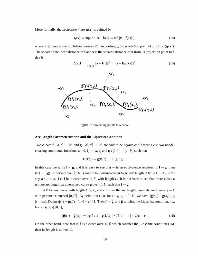
More formally, the projection index tf(x) is defined by

tf(x) = sup{

t : ‖x− f(t)‖ = infτ‖x− f(τ)‖

}

, (14)

where ‖ · ‖ denotes the Euclidean norm in Rd . Accordingly, the projection point of x to f is f(tf(x)).

The squared Euclidean distance of f and x is the squared distance of x from its projection point to f,

that is,

∆(x, f) = infa≤t≤b

‖x− f(t)‖2 = ‖x− f(tf(x))‖2. (15)

��

��

��

��

�

�

� ��

��

��

��

��

��

��

��

��

��

��

��

��

��

x1

f f 1 (t (x ))f f 2 (t (x ))

2f f 3

x4

f f 4 (t (x ))x5

f f 5 (t (x ))x3

x6

f f 6 (t (x ))f f 7 (t (x ))

x7

(t (x ))x

Figure 2: Projecting points to a curve.

Arc Length Parameterization and the Lipschitz Condition

Two curves f : [a,b] → Rd and g : [a′,b′] → R

d are said to be equivalent if there exist two nonde-

creasing continuous functions φ : [0,1] → [a,b] and η : [0,1] → [a′,b′] such that

f(φ(t)) = g(η(t)), 0 ≤ t ≤ 1.

In this case we write f ∼ g, and it is easy to see that ∼ is an equivalence relation. If f ∼ g, then

l(f) = l(g). A curve f over [a,b] is said to be parameterized by its arc length if l(f,a, t) = t −a for

any a ≤ t ≤ b. Let f be a curve over [a,b] with length L. It is not hard to see that there exists a

unique arc length parameterized curve g over [0,L] such that f ∼ g.

Let f′ be any curve with length L′ ≤ L, and consider the arc length parameterized curve g ∼ f′

with parameter interval [0,L′]. By definition (13), for all s1,s2 ∈ [0,L′] we have ‖g(s1)− g(s2)‖ ≤|s1− s2|. Define g(t) = g(L′t) for 0 ≤ t ≤ 1. Then f′ ∼ g, and g satisfies the Lipschitz condition, i.e.,

For all t1, t2 ∈ [0,1],

‖g(t1)− g(t2)‖ = ‖g(L′t1)−g(L′t2)‖ ≤ L′|t1 − t2| ≤ L|t1 − t2|. (16)

On the other hand, note that if g is a curve over [0,1] which satisfies the Lipschitz condition (16),

then its length is at most L.

19

Note that if l(f) < ∞, then by the continuity of f, its graph

Gf = f([a,b]) = {f(t) : a ≤ t ≤ b} (17)

is a compact subset of Rd , and the infimum in (15) is achieved for some t. Also, since Gf = Gg if

f ∼ g, we also have that ∆(x, f) = ∆(x,g) for all g ∼ f.

Geometrical Properties of Curves

Let f : [a,b]→Rd be a differentiable curve with f = ( f1, . . . , fd). The velocity of the curve is defined

as the vector function

f′(t) =

(

d f1

dt(t), . . . ,

d fd

dt(t)

)

.

It is easy to see that f′(t) is tangent to the curve at t and that for an arc length parameterized curve

‖f′(t)‖ ≡ 1. Note that for a differentiable curve f : [a,b] → Rd , the length of the curve (13) over an

interval [α,β] ⊂ [a,b] can be defined as

l(f,α,β) =Z β

α‖f′(t)‖dt.

The vector function

f′′(t) =

(

d2 f1

dt2 (t), . . . ,d2 fd

dt2 (t)

)

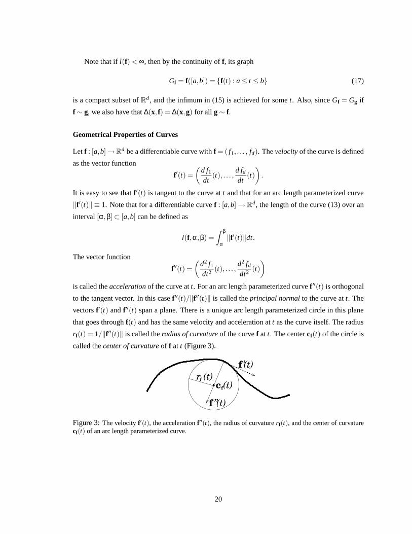
is called the acceleration of the curve at t. For an arc length parameterized curve f′′(t) is orthogonal

to the tangent vector. In this case f′′(t)/‖f′′(t)‖ is called the principal normal to the curve at t. The

vectors f′(t) and f′′(t) span a plane. There is a unique arc length parameterized circle in this plane

that goes through f(t) and has the same velocity and acceleration at t as the curve itself. The radius

rf(t) = 1/‖f′′(t)‖ is called the radius of curvature of the curve f at t. The center cf(t) of the circle is

called the center of curvature of f at t (Figure 3).

c

’

f ’’

��

f

f (t)��

��

f r (t)(t)

(t)

Figure 3: The velocity f′(t), the acceleration f′′(t), the radius of curvature rf(t), and the center of curvaturecf(t) of an arc length parameterized curve.

20

The Distance Function and the Empirical Distance Function

Consider a d-dimensional random vector X = (X1, . . . ,Xd) with finite second moments. The distance

function of a curve f is defined as the expected squared distance between X and f, that is,

∆(f) = E[

∆(X, f)]

= E[

inft‖X− f(t)‖2]= E

[

‖X− f(tf(X))‖2]. (18)

In practical situations the distribution of X is usually unknown, but a data set Xn = {x1, . . . ,xn}⊂R

d drawn independently from the distribution is known instead. In this case, we can estimate the

distance function of a curve f by the empirical distance function defined as

∆n(f) =1n

n

∑i=1

∆(xi, f). (19)

Straight Lines and Line Segments

Consider curves of the form

s(t) = tu+ c

where u,c ∈Rd , and u is a unit-vector. If the domain of t is the real line, s is called a straight line, or

line. If s is defined on a finite interval [a,b] ⊂ R, s is called a straight line segment, or line segment.

Note that since ‖u‖ = 1, s is arc length parameterized.

By (15), the squared distance of a point x and a line s is

∆(x,s) = inft∈R

‖x− s(t)‖2

= inft∈R

‖x− (tu+ c)‖2

= ‖x− c‖2 + inft∈R

(

t2 −2t(x− c)T u)

= ‖x− c‖2 − ((x− c)T u)2 (20)

where xT denotes the transpose of x. The projection point of x to s is c+((x− c)T u)u.

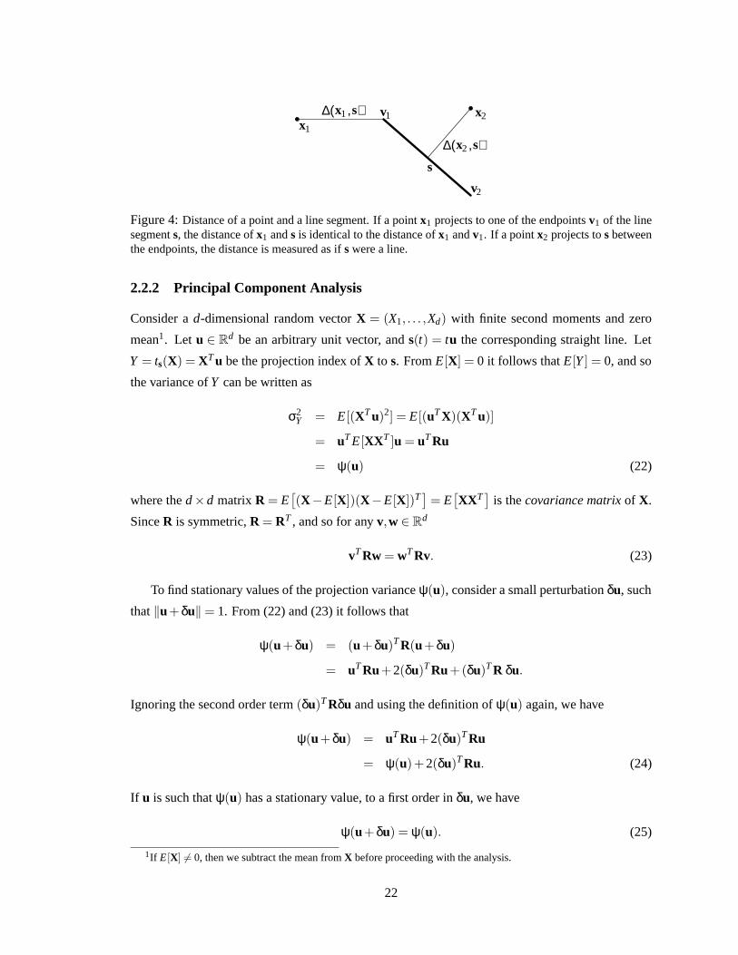
If s(t) = tu + c is a line segment defined over [a,b] ⊂ R, the way the distance of a point x and

the line segment is measured depends on the value of the projection index ts(x). If ts(x) = a or

ts(x) = b, the distance is measured as the distance of x and one of the endpoints v1 = au + c or

v2 = bu + c, respectively. If x projects to s between the endpoints, the distance is measured as if s

were a line (Figure 4). Formally,

∆(x,s) =

‖x−v1‖2 if s(ts(x)) = v1,

‖x−v2‖2 if s(ts(x)) = v2,

‖x− c‖2 − ((x− c)T u)2 otherwise.

(21)

21

∆( , )

∆( , )

x2 s

x

s

v1 x2

v2

1

s1x

Figure 4: Distance of a point and a line segment. If a point x1 projects to one of the endpoints v1 of the linesegment s, the distance of x1 and s is identical to the distance of x1 and v1. If a point x2 projects to s betweenthe endpoints, the distance is measured as if s were a line.

2.2.2 Principal Component Analysis

Consider a d-dimensional random vector X = (X1, . . . ,Xd) with finite second moments and zero

mean1. Let u ∈ Rd be an arbitrary unit vector, and s(t) = tu the corresponding straight line. Let

Y = ts(X) = XT u be the projection index of X to s. From E[X] = 0 it follows that E[Y ] = 0, and so

the variance of Y can be written as

σ2Y = E[(XT u)2] = E[(uT X)(XT u)]

= uT E[XXT ]u = uT Ru

= ψ(u) (22)

where the d ×d matrix R = E[

(X−E[X])(X−E[X])T]

= E[

XXT]

is the covariance matrix of X.

Since R is symmetric, R = RT , and so for any v,w ∈ Rd

vT Rw = wT Rv. (23)

To find stationary values of the projection variance ψ(u), consider a small perturbation δu, such

that ‖u+δu‖ = 1. From (22) and (23) it follows that

ψ(u+δu) = (u+δu)T R(u+δu)

= uT Ru+2(δu)T Ru+(δu)T R δu.

Ignoring the second order term (δu)T Rδu and using the definition of ψ(u) again, we have

ψ(u+δu) = uT Ru+2(δu)T Ru

= ψ(u)+2(δu)T Ru. (24)

If u is such that ψ(u) has a stationary value, to a first order in δu, we have

ψ(u+δu) = ψ(u). (25)

1If E[X] 6= 0, then we subtract the mean from X before proceeding with the analysis.

22

Hence, (25) and (24) imply that

(δu)T Ru = 0. (26)

Since ‖u+δu‖2 = ‖u‖2 +2(δu)T u+‖δu‖2 = 1, we require that, to a first order in δu,

(δu)T u = 0. (27)

This means that the perturbation δu must be orthogonal to u. To find a solution of (26) with the

constraint (27), we have to solve

(δu)T Ru− l(δu)T u = 0,

or, equivalently,

(δu)T (Ru− lu) = 0. (28)

For the condition (28) to hold, it is necessary and sufficient that we have

Ru = lu. (29)

The solutions of (29), l1, . . . , ld , are the eigenvalues of R, and the corresponding unit vectors,

u1, . . . ,ud , are the eigenvectors of R. For the sake of simplicity, we assume that the eigenvalues are

distinct, and they are indexed in decreasing order, i.e.,

l1 > .. . > ld .

Define the d ×d matrix U as

U = [u1, . . . ,ud],

and let be the diagonal matrix

= diag[l1, . . . , ld].

Then the d equations of form (29) can be summarized in

RU = U . (30)

The matrix U is orthonormal so U−1 = UT , and therefore (30) can be written as

UT RU = . (31)

Thus, from (22) and (31) it follows that the principal directions along which the projection variance

is stationary are the eigenvectors of the covariance matrix R, and the stationary values themselves

are the eigenvalues of R. (31) also implies that the maximum value of the projection variance is the

23

largest eigenvalue of R, and the principal direction along which the projection variance is maximal

is the eigenvector associated with the largest eigenvalue. Formally,

max‖u‖=1

ψ(u) = l1, (32)

and

argmax‖u‖=1

ψ(u) = u1. (33)

The straight lines si(t) = tui, i = 1, . . . ,d are called the principal component lines of X. Since the

eigenvectors form an orthonormal basis of Rd , any data vector x ∈ R

d can be represented uniquely

by its projection indices ti = uTi x, i = 1, . . . ,d to the principal component lines. The projection in-

dices ti, . . . , td are called the principal components of x. The construction of the vector t = [ti, . . . , td]T

of the principal components,

t = UT x,

is the principal component analysis of x. To reconstruct the original data vector x from t, note again

that U−1 = UT so

x = (UT )−1t = Ut =d

∑i=1

tiui. (34)

From the perspective of feature extraction and data compression, the practical value of princi-

pal component analysis is that it provides an effective technique for dimensionality reduction. In

particular, we may reduce the number of parameters needed for effective data representation by dis-

carding those linear combinations in (34) that have small variances and retain only those terms that

have large variances. Formally, let §d′ be the d′-dimensional linear subspace spanned by the first d ′

eigenvectors of R. To approximate X, we define

X′ =d′

∑i=1

tiui,

the projection of X to §d′ . It can be shown by using (33) and induction that §d′ maximizes the

variance of X′,

E[

X′2]=d′

∑i=1

ψ(ui) =d′

∑i=1

li,

and minimizes the variance of X−X′,

E[

(X−X′)2]=d

∑i=d′+1

ψ(ui) =d

∑i=d′+1

li,

among all d′-dimensional linear subspaces. In other words, the solutions of both Problem 1 and

Problem 2 are the subspace which is spanned by the first d ′ eigenvectors of X’s covariance matrix.

24

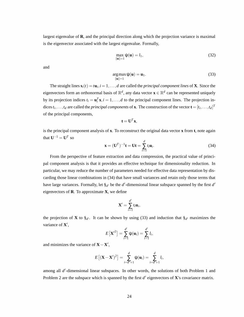
2.2.3 Properties of the First Principal Component Line

The first principal component line (Figure 5) of a random variable X with zero mean is defined as

the straight line s1 = tu1 where u1 is the eigenvector which belongs to the largest eigenvalue l1 of

X’s correlation matrix. The first principal component line has the following properties.

1. The first principal component line maximizes the variance of the projection of X to a line

among all straight lines.

2. The first principal component line minimizes the distance function among all straight lines.

3. If the distribution of X is elliptical, the first principal component line is self-consistent, that is,

any point of the line is the conditional expectation of X over those points of the space which

project to this point. Formally,

s1(t) = E[

X|tf(X) = t]

.

Figure 5: The first principal component line of an elliptical distribution in the plane.

Property 1 is a straightforward consequence of (33). To show Property 2, note that if s(t)= tu+c

is an arbitrary straight line, then by (18) and (20),

∆(s) = E[

∆(X,s)]

= E[

‖X− c‖2 − ((X− c)T u)2]

= E[

‖X‖2]+‖c‖2 −E[

(XT u)2]− (cT u)2 (35)

= σ2X −ψ(u)+‖c‖2 − (cT u)2

≤ σ2X −ψ(u), (36)

where (35) follows from E[X] = 0. On the one hand, in (36) equality holds if and only if c = tu

for some t ∈ R. Geometrically, it means that the minimizing line must go through the origin. On

25

the other hand, σ2X −ψ(u) is minimized when ψ(u) is maximized, that is, when u = u1. These two

conditions together imply Property 2. Property 3 follows from the fact that the density of a random

variable with an elliptical distribution is symmetrical about the principal component lines.

2.2.4 A Fast PCA Algorithm for Data Sets

In practice, principal component analysis is usually applied for sets of data points rather than dis-

tributions. Consider a data set Xn = {x1, . . . ,xn} ⊂ Rd , such that 1

n ∑ni=1 xn = 0. The first principal

component line of Xn is a straight line s1(t) = tu1 that minimizes the empirical distance function

(19),

∆n(s) =1n

n

∑i=1

∆(xi,s),

among all straight lines. The solution lies in the eigenstructure of the sample covariance matrix of

the data set, which is defined as Rn = 1n ∑n

i=1 xnxTn . Following the derivation of PCA for distributions

previously in this section, it can be shown easily that the unit vector u1 that defines the minimizing

line s1 is the eigenvector which belongs to the largest eigenvalue of Rn.

An obvious algorithm to minimize ∆n(s) is therefore to find the eigenvectors and eigenvalues of

Rn. The crude method, direct diagonalization of Rn, can be extremely costly for high-dimensional

data since it takes O(nd3) operations. More sophisticated techniques, for example the power method

(e.g., see [Wil65]), exist that perform matrix diagonalization in O(nd2) steps if only the first leading

eigenvectors and eigenvalues are required. Since the d × d covariance matrix Rn must explicitly

be computed, O(nd2) is also the theoretical lower limit of the computational complexity of this

approach.

To break the O(nd2) barrier, several approximative methods were proposed (e.g., [Oja92],

[RT89], [Fol89]). The common approach of these methods is to start from an arbitrary line, and

to iteratively optimize the orientation of the line using the data so that it converges to the first princi-

pal component line. The characterizing features of these algorithms are the different learning rules

they use for the optimization in each iteration.

The algorithm we introduce here is of the same genre. It was proposed recently, independently

by Roweis [Row98] and Tipping and Bishop [TB99]. The reason we present it here is that there is a

strong analogy between this algorithm designed for finding the first principal component line2, and

the HS algorithm (Section 3.1.1) for computing principal curves of data sets. Moreover, we also use

a similar method in the inner iteration of the polygonal line algorithm (Section 5.1) to optimize the

locations of vertices of the polygonal principal curve.

2The original algorithm in [Row98] and [TB99] can compute the first d′ principal components simultaneously. Forthe sake of simplicity, we present it here only for the first principal component line.

26

The basic idea of the algorithm is the following. Start with an arbitrary straight line, and project

all the data points to the line. Then fix the projection indices, and find a new line that optimizes the

distance function. Once the new line has been computed, restart the iteration, and continue until

convergence.

Formally, let s( j)(t) = tu( j) be the line produced by the jth iteration, and let t( j) =[

t( j)1 , . . . , t( j)

n

]T=

[

xT1 u( j), . . . ,xT

n u( j)]T

be the vector of projection indices of the data points to s( j). The distance func-

tion of s(t) = tu assuming the fixed projection vector t( j) is defined as

∆n

(

s∣

∣

∣t( j))

= =n

∑i=1

∥

∥

∥xi − t( j)

i u∥

∥

∥

2

=n

∑i=1

‖xi‖2 +‖u‖2n

∑i=1

(

t( j)i

)2−2uT

n

∑i=1

t( j)i xi. (37)

Therefore, to find the optimal line s( j+1), we have to minimize (37) with the constraint that ‖u‖= 1.

It can be shown easily that the result of the constrained minimization is

u( j+1) = argmin‖u‖=1

∆(

s∣

∣

∣t( j))

=∑n

i=1 t( j)i xi

∥

∥

∥∑ni=1 t( j)

i xi

∥

∥

∥

,

and so s( j+1)(t) = tu( j+1).

The formal algorithm is the following.

Algorithm 3 (The RTB algorithm)

Step 0 Let s(0)(t) = tu(0) be an arbitrary line. Set j = 0.

Step 1 Set t( j) =[

t( j)1 , . . . , t( j)

n

]T=[

xT1 u( j), . . . ,xT

n u( j)]T

.

Step 2 Define u( j+1) = ∑ni=1 t( j)

i xi∥

∥

∥∑ni=1 t( j)

i xi

∥

∥

∥

, and s( j+1)(t) = tu( j+1).

Step 3 Stop if

(

1− ∆n(s( j+1))∆n(s( j))

)


Step 1.

The standard convergence proof for the Expectation-Minimization (EM) algorithm [DLR77]

applies to the RTB algorithm so it can be shown that s( j) has a limit s(∞), and that the distance

function ∆n (s) has a local maximum in s(∞). Furthermore, [TB99] showed that the only stable local

extremum is the global maximum so s(∞) is indeed the first principal component line.

27

Chapter 3

Principal Curves and Related Areas

In this chapter we introduce the original HS definition of principal curves and summarize some

of the subsequent research. We also describe the connection of principal curves to some of the

related unsupervised learning models. Section 3.1 introduces the HS definition of principal curves,

and describes the HS algorithm for probability distributions and data sets. Section 3.2 summarizes

some of the subsequent results on principal curves and highlights the relationship between principal

curves, self-organizing maps and nonlinear principal component analysis.

3.1 Principal Curves with Self-Consistency Property

3.1.1 The HS Definition

Property 3 in Section 2.2 states that for elliptical distributions the first principal component is self-

consistent, i.e., any point of the line is the conditional expectation of X over those points of the space

which project to this point. HS generalized the self-consistency property of principal components

and defined principal curves as follows.

Definition 2 The smooth curve f(t) is a principal curve if the following hold:

(i) f does not intersect itself,

(ii) f has finite length inside any bounded subset of Rd ,

(iii) f is self-consistent, i.e., f(t) = E[

X|tf(X) = t]

.

Intuitively, self-consistency means that each point of f is the average (under the distribution of X)

of all points that project there. Thus, principal curves are smooth self-consistent curves which pass

through the “middle” of the distribution and provide a good one-dimensional nonlinear summary of

the data (see Figure 6).

28

��

��

��

�� !�!"�" #�#$

%�%& '�'(�(

)�)*�*+�+,�,

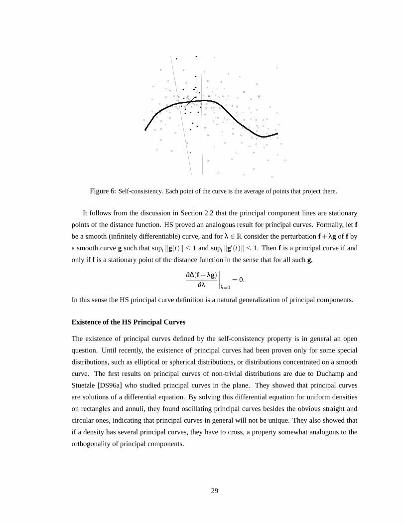
-./�/0�01�12�2

3456

789:;<

=>

Figure 6: Self-consistency. Each point of the curve is the average of points that project there.

It follows from the discussion in Section 2.2 that the principal component lines are stationary

points of the distance function. HS proved an analogous result for principal curves. Formally, let f

be a smooth (infinitely differentiable) curve, and for λ ∈ R consider the perturbation f + λg of f by

a smooth curve g such that supt ‖g(t)‖ ≤ 1 and supt ‖g′(t)‖ ≤ 1. Then f is a principal curve if and

only if f is a stationary point of the distance function in the sense that for all such g,

∂∆(f+λg)

∂λ

∣

∣

∣

∣

λ=0= 0.

In this sense the HS principal curve definition is a natural generalization of principal components.

Existence of the HS Principal Curves

The existence of principal curves defined by the self-consistency property is in general an open

question. Until recently, the existence of principal curves had been proven only for some special

distributions, such as elliptical or spherical distributions, or distributions concentrated on a smooth

curve. The first results on principal curves of non-trivial distributions are due to Duchamp and

Stuetzle [DS96a] who studied principal curves in the plane. They showed that principal curves

are solutions of a differential equation. By solving this differential equation for uniform densities

on rectangles and annuli, they found oscillating principal curves besides the obvious straight and

circular ones, indicating that principal curves in general will not be unique. They also showed that

if a density has several principal curves, they have to cross, a property somewhat analogous to the

orthogonality of principal components.

29

The HS Algorithm for Distributions

Based on the self-consistency property, HS developed an algorithm for constructing principal curves.

Similar in spirit to the GL algorithm of vector quantizer design (Section 2.1), and the RTB algorithm

(Section 2.2.4) of principal component analysis, the HS algorithm iterates between a projection step

and an expectation step until convergence. In the projection step, projection indices of the data to

the curve are computed. In the expectation step, a new curve is computed. For every point f( j)(t) of

the previous curve, a point of the new curve is defined as the expectation of the data that project to

f( j)(t). When the probability density of X is known, the formal algorithm for constructing principal

curves is the following.

Algorithm 4 (The HS algorithm)

Step 0 Let f(0)(t) be the first principal component line for X. Set j = 0.

Step 1 (Projection) Set tf( j)(x) = max{t : ‖x− f(t)‖ = minτ ‖x− f(τ)‖} for all x ∈ Rd .

Step 2 (Expectation) Define f( j+1)(t) = E [X|tf( j)(X) = t].

Step 3 Stop if

(

1− ∆(f( j+1))∆(f( j))

)


Step 1.

Although HS is unable to prove that the algorithm converges, they have the following evidence

in its favor:

1. By definition, principal curves are fixed points of the algorithm.

2. Assuming that each iteration is well defined and produces a differentiable curve, the expected

squared distance ∆(f) converges.

3. If Step 1 is replaced by fitting a least squares straight line, then the procedure converges to

the largest principal component.

Unfortunately, the fact that ∆(f) converges does not mean that f converges to any meaningful so-

lution. Among the principal components, the largest principal component minimizes the distance

function, the smallest principal component maximizes it, and all the others are saddle points. Inter-

estingly, there is no such distinction between different principal curves of a distribution. [DS96b]

showed that all principal curves are saddle points of the distance function. In this sense, any algo-

rithm that aims to find a principal curve by minimizing the distance function will fail to converge

to a stable solution without further restricting the set of admissible curves. This fact is one of the

motivations behind our new definition of principal curves in Chapter 4.

30

3.1.2 The HS Algorithm for Data Sets

Similarly to the GL and RTB algorithms, the HS algorithm can be extended to data sets. Unlike

in the former two cases, however, this case requires more than simple replacements of expectations

by the corresponding sample averages. A general issue is the representation of the curve by a finite

number of parameters. A more serious problem arises in the expectation step: in general there is at

most one point that projects to a given point of the curve. In this section we give a detailed treatment

of the modifications proposed by HS, and analyze the algorithm.

Assume that a set of points Xn = {x1, . . . ,xn} ⊂ Rd is given. Project the data points to an

arbitrary curve f, and index the points so that their projection indices t1, . . . , tn are in increasing

order. We can represent the curve f by a polygonal curve of n vertices by connecting pairs of

consecutive projection points (f(ti), f(ti+1)) , i = 1, . . . ,n− 1 by line segments. In the discussion

below we assume that all curves produced by the algorithm are such polygonal curves. We also

assume that all curves are arc length parameterized, so the parameters ti, i = 1, . . . ,n can be defined

recursively by

1. t1 = 0,

2. ti = ti−1 +‖f(ti)− f(ti−1)‖, i = 2, . . . ,n.(38)

In Step 0, f(0)(t) is the first principal component line of the data set Xn. In the stopping condition

in Step 3, the distance function ∆(

f( j+1))

is replaced by the empirical distance function,

∆n

(

f( j+1))

=1n

n

∑i=1

∥

∥

∥xi − f( j+1)

(

t( j)i

)∥

∥

∥

2.

In the projection step (Step 1), the new projection indices t ( j)i , i = 1, . . . ,n are computed by projecting

the data points to f( j)(t). When we reach this step for the first time, the projection indices can be set

by projecting the data points to the first principal component line. After the jth iteration, the current

curve is represented as a polygonal curve of vertices f( j)(

t( j−1)1

)

, . . . , f( j)(

t( j−1)n

)

. Let s` be the line

segment that connects the vertices f( j)(

t( j−1)`

)

and f( j)(

t( j−1)`+1

)

, ` = 1, . . . ,n− 1. To compute the

projection index of a data point xi, we have to find the nearest line segment to xi, denoted by s`(i),

where the index `(i) is defined by

`(i) = argmin`=1,...,n−1

∆(xi,s`).

If s`(i) is defined over[

t( j−1)`(i) , t( j−1)

`(i)+1

]

, the new projection index is identical to the projection index

of xi to s`(i), that is,

t( j)i = ts`(i)

(xi).

Figure 7 illustrates the method for a data point.

31

xi

f f i (t (x ))

Figure 7: Computing projection points. xi is projected to the line segments (along the solid thin lines), andthe nearest projection point is chosen (connected to xi by dashed line). Note that the nearest vertex (connectedto xi by dotted line) is not the endpoint of the nearest line segment.

There seems to be a simpler approach to find the projection point of a data point xi. Instead

of searching through the line segments, one could find the nearest vertex to xi, project the point

to the vertex and the two incident line segments, and pick the nearest projection. Figure 7 clearly

indicates that this approach can yield a wrong result if the nearest vertex of the polygonal curve is

not the endpoint of nearest line segment. Although this configuration occurs quite rarely, in general

it cannot be excluded.

Before proceeding with expectation step, the data points are reindexed in increasing order by

their projection indices.

In the expectation step (Step 2), finite points of the new curve f( j+1)(t) = E[

X|tf( j)(X) = t]

are

estimated at the n projection indices t = t ( j)1 , . . . , t( j)

n found in the projection step. In general, the only

observation that projects to f( j)(t) at t( j)i is xi. Using this one point in the averaging would result in a

curve that visits all the data points after the first iteration. To tackle this problem, HS proposed two

approaches. In the first, E[

X|tf( j)(X) = t( j)i

]

is estimated by averaging over observations that project

close to t( j)i . HS used the locally weighted running-lines smoother [Cle79] for local averaging. In

the second approach, a non-parametric regression estimate (cubic smoothing splines [Sil85]) is used

to minimize a data-dependent criteria.

Locally Weighted Running-Lines Smoother

Consider the estimation of the single coordinate function E[

X |tf( j)(X) = t( j)i

]

based on the sample

of n pairs (t( j)1 ,x1), . . . ,(t

( j)n ,xn). To estimate this quantity, the smoother fits a straight line to the first

wn observations {xk} of which the projection index t( j)k is the closest to t( j)

i . The estimate is taken to

be the fitted value of the line at t( j)i . The fraction w of points in the neighborhood is called the span,

and w is a parameter of the smoother. In fitting the line, weighted least squares regression is used.

32

The weights are derived from a symmetric kernel centered at t ( j)i that goes smoothly to 0 within

the neighborhood. Formally, let t ( j)w denote the wnth nearest projection index to t ( j)

i , and define the

weight wik of the observation xk by

wik =

(

1−∣

∣

∣

∣

t( j)k −t( j)

i

t( j)w −t( j)

i

∣

∣

∣

∣

3)1/3

if∣

∣

∣t( j)k − t( j)

i

∣

∣

∣<∣

∣

∣t( j)w − t( j)

i

∣

∣

∣,

0 otherwise.

(39)

Cubic Smoothing Splines

The algorithm to estimate principal curves for data sets is motivated by the algorithm for finding

principal curves of distributions, so it is designed to find a stationary point of the average squared

distance, ∆n(f) = 1n ∑n

i=1 ‖xi − f(tf(xi))‖2. To obtain a smooth curve solution, motivated by cubic

smoothing splines [Sil85], HS suggested to minimize a penalized average squared distance criterion

to define principal curves. Formally, let

G(f) = ∆n(f)+µP(f), (40)

where P(f) =R 1

0 ‖f′′(τ)‖2dτ measures the total curvature of the curve, and the penalty coefficient

µ is a parameter of the algorithm. Note that the parameter of the curve is rescaled to lie in the

interval [0,1]. In the expectation step the criteria (40) is minimized by minimizing separately the d

coordinate functions,

G( f`) =1n

n

∑i=1

|xi`− f`(ti)|2 +µZ 1

0| f ′′` (τ)|2dτ, ` = 1, . . . ,d.

Computational Complexity of the HS Algorithm

In the projection step the distance between n line segments and n data points is computed, so the

complexity of the step is O(n2). The computational complexity of the expectation step is O(n2) for

the kernel type smoothers, and O(n) for the smoothing spline. The complexity of the sorting routine

after the projection step is O(n logn). Hence, the computational complexity of the HS algorithm,

dominated by the complexity of the projection step, is O(n2).1

3.1.3 The Bias of the HS Algorithm

HS observed two sources of bias in the estimation process. Model bias occurs when data points are

generated by the additive model

X = f(Y )+ e (41)

1[Has84] argues that the computational complexity of the projection step can be improved by using spatial datastructures. [YMMS92] claims similar results. However, both [Has84] and [YMMS92] attempt to find the projectionpoint x of a data point by finding the nearest vertex to x, and projecting x to the two line segments incident to the vertex.As we showed earlier in this section, in general, this approach can yield a wrong result.

33

where Y is uniformly distributed over the domain of the smooth curve f, and e is bivariate additive

noise which is independent of Y . In general, if f has a curvature, it is not self-consistent so it is not

a principal curve of the distribution of X. The self-consistent curve lies outside f from the point of

view of the center of the curvature. This bias goes to 0 with the ratio of the noise variance and the

radius of the curvature.

Estimation bias occurs because the scatterplot smoothers average over neighborhoods. The

estimation bias points towards the center of curvature so usually it has a flattening effect on the

estimated curve. Unlike the model bias, the estimation bias can be affected by parameters of the

algorithm. The larger the span coefficient w of the running-lines smoother or the penalty coefficient

µ of the spline smoother, the larger is the bias. So, in theory it is possible to set these parameters so

that the two bias components cancel each other.

HS proposed a simple model for the quantitative analysis of the two bias components. Let f be

an arc length parameterized circle with constant curvature 1/r, i.e, let

f(t) =

[

r cos(t/r)

r sin(t/r)

]

for t ∈ I = [−rπ,rπ). Let the random variable X be defined by (41). Assume that the noise e has

zero mean and σ2 variance in both coordinates. HS showed that in this situation the radius r∗ of

the self-consistent circle f∗ is larger than r. The intuitive explanation of this is that the model (41)

seems to generate more mass outside the circle f than inside (Figure 8(a)). In a quantitative analysis,

HS showed that, under certain conditions,

r∗ ≈ r +σ2

2r(42)

so the bias inherent in the model (41) is σ2/2r. It also follows from the analysis that the distance

function at f∗ is

∆(f∗) ≈ σ2 − σ4

4r2 = ∆(f)− σ4

4r2 . (43)

The source of the estimation bias is the local averaging procedure used in the HS algorithm

designed for data sets. Assume that the principal curve at t = 0 is estimated by using data that

projects to the curve in the interval Iθ = [−rθ,rθ] (Figure 8(b)). The smoother fits a straight line to

the data, and the estimate is taken to be the fitted value of the line at t = 0. Clearly, the estimate will

be inside the generating curve. HS showed that under certain conditions the radius of the estimated

curve is

rθ = r∗sin(θ/2)

θ/2. (44)

34

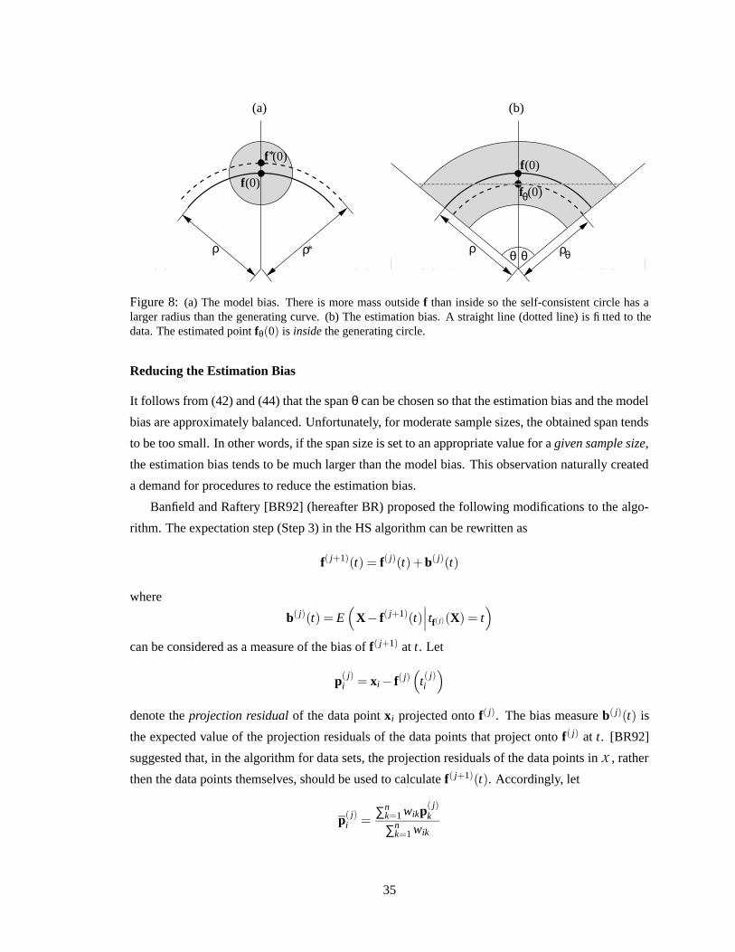
(a)

(0)

f*(0)

ρ*

f

ρ

(b)

f(0)

(0)fθ

ρθρ θ θ

Figure 8: (a) The model bias. There is more mass outside f than inside so the self-consistent circle has alarger radius than the generating curve. (b) The estimation bias. A straight line (dotted line) is fitted to thedata. The estimated point fθ(0) is inside the generating circle.

Reducing the Estimation Bias

It follows from (42) and (44) that the span θ can be chosen so that the estimation bias and the model

bias are approximately balanced. Unfortunately, for moderate sample sizes, the obtained span tends

to be too small. In other words, if the span size is set to an appropriate value for a given sample size,

the estimation bias tends to be much larger than the model bias. This observation naturally created

a demand for procedures to reduce the estimation bias.

Banfield and Raftery [BR92] (hereafter BR) proposed the following modifications to the algo-

rithm. The expectation step (Step 3) in the HS algorithm can be rewritten as

f( j+1)(t) = f( j)(t)+b( j)(t)

where

b( j)(t) = E(

X− f( j+1)(t)∣

∣

∣tf( j)(X) = t

)

can be considered as a measure of the bias of f( j+1) at t. Let

p( j)i = xi − f( j)

(

t( j)i

)

denote the projection residual of the data point xi projected onto f( j). The bias measure b( j)(t) is

the expected value of the projection residuals of the data points that project onto f( j) at t. [BR92]

suggested that, in the algorithm for data sets, the projection residuals of the data points in X , rather

then the data points themselves, should be used to calculate f( j+1)(t). Accordingly, let

p( j)i =

∑nk=1 wikp( j)

k

∑nk=1 wik

35

be the weighted average of the projection residuals of the data points that project close to t ( j)i . By

using p( j)i as the estimation of the bias b( j)

(

t( j)i

)

, the new point of the curve is estimated by

f( j+1)(

t( j)i

)

= f( j)(

t( j)i

)

+p( j)i .

[BR92] also extended the HS algorithm to closed curves. Experimental results on simulated

data are given in Section 5.2, where the HS algorithm with smoothing splines is compared to the

BR algorithm and the polygonal line algorithm introduced in Section 5.1.

3.2 Alternative Definitions and Related Concepts

3.2.1 Alternative Definitions of Principal Curves

Two substantially different approaches to principal curves have been proposed subsequent to Hastie

and Stuetzle’s groundbreaking work. Tibshirani [Tib92] introduced a semi-parametric model for

principal curves. The motivation of [Tib92] to redefine principal curves is the unsettling property

of the HS principal curves that if the distribution of the data is defined by the additive model X =

f(Y ) + e (see (41)), f is not the principal curve of X in general. To solve this problem, [Tib92]

derives principal curves from the additive model (41). Consider a d-dimensional random vector

X = (X1, . . . ,Xd) with density µX. Now imagine that X was generated in two stages. In the first step,

a point on a curve f(Y ) is generated according to some distribution µY , and in the second step, X

is generated from a conditional distribution µX|Y where the mean of µX|Y is f(Y ), and X1, . . . ,Xd are

conditionally independent given Y . Using this model, [Tib92] defines principal curves as follows.

Definition 3 The principal curve of a random variable X is a triplet {µY ,µX|Y , f} satisfying the

following conditions:

(i) µY and µX|Y are consistent with µX, that is, µX(x) =R

µX|Y (x|y)µY (y)dy.

(ii) X1, . . . ,Xd are conditionally independent given Y .

(iii) f(t) is a curve in Rd parameterized over a closed interval in R satisfying f(t) = E[X|Y = t].

It is easy to see that if the distribution of the data is defined by the additive model (41), the

generating curve f is indeed the principal curve of X in the sense of Definition 3. Based on this

definition, [Tib92] proposed a semi-parametric scheme for estimating principal curves of data sets.

In the model, µY is left completely unspecified, while µX|Y is assumed to be from a parametric

family. Therefore, at a certain parameter y, one has to estimate the point of the curve f(y) and the

36

parameters Σ(y) of µX|Y . Given a data set Xn = {x1, . . . ,xn}⊂Rd , [Tib92] uses maximum likelihood

estimation to find the unknown parameters. The log-likelihood

l(f,Σ) =n

∑i=1

logZ

µX|Y (xi|f(y),Σ(y))µY (y)dy

was minimized by using the EM algorithm [DLR77]. The algorithm was tested on several simulated

and real data sets and compared to the HS algorithm. Although Definition 3 has some theoretical

advantages over the HS definition, the resulting estimation procedure does not produce better results

than the HS algorithm.

Recently, Delicado [Del98] proposed yet another definition based on a property of the first

principal components of multivariate normal distributions. Consider a d-dimensional random vector

X = (X1, . . . ,Xd). [Del98] calls a point x∗ ∈ Rd a principal oriented point if there exists a direction

u∗(x∗) ∈ Rd such that x∗ is the conditional mean of X in the hyperplane orthogonal to u∗(x∗) that

contains x∗, i.e.,

x∗ = E[

X|(X−x∗)T u∗(x) = 0]

.

A curve f : [a,b]→ Rd is called a principal curve of oriented points of X if for all t ∈ [a,b], the points

of the curve f(t) are principal oriented points. The definition can be considered as a generalization

of PCA since the first principal component of a multivariate normal distribution is a principal curve

of oriented points. It can be seen easily that if the curve f satisfies certain regularity conditions,

namely that no points of the support of the distribution of X can be projected orthogonally to more

than one points of f, then f is a principal curve of oriented points if and only if it is a principal curve

in the HS sense. [Del98] also proposed an algorithm to find a principal curve of oriented points of a

given data set. Examples indicate that the curves produced by the procedure tend to be less smooth

than the curves produced by the HS algorithm.

3.2.2 The Self-Organizing Map

Kohonen’s self-organizing map (SOM) [Koh82] is one of the most widely used and most exten-

sively studied unsupervised learning method. The basic idea of the algorithm was inspired by the

way the brain forms topology preserving neural representations or maps of various sensory impres-

sions. Keys of the success of the SOM among practitioners are its simplicity, efficiency, and low

computational complexity.

In a certain sense, the SOM algorithm can be considered as a generalization of both the GL al-

gorithm and the HS algorithm (with local averaging). The relation of SOM and vector quantization

is a widely known fact (see, e.g. [Koh97]), whereas the similarities between SOM and principal

curves were pointed out recently by [RMS92] and [MC95]. The SOM algorithm is usually formu-

lated as a stochastic learning algorithm. To emphasize its similarities to the HS and GL algorithms,

37

we present it here as a batch method as it was first formulated by Luttrell [Lut90].

In its original form, the SOM is a nearest neighbor vector quantizer equipped with a topology.

Similarly to vector quantization, we are given a set of codepoints C = {v1, . . . ,vk}⊂Rd . In addition,

there is a weighted graph defined over C by a k× k matrix of weights W = {w`,m}. The weights

w`,m (`,m = 1, . . . ,k) are usually defined as a monotonically decreasing function of the Euclidean

distance between the initial codepoints v` and vm. In this sense, W can be considered as a topology

over C . In the simplest case, codepoints are organized in a one-dimensional topology, typically

along a line. In practice, the topology is usually two-dimensional, i.e., initial codepoints are placed

in a rectangular or hexagonal grid. Three or more-dimensional topologies are rarely used.

The objective of the SOM algorithm is to fit the map to a data set X = {x1, . . . ,xn} ⊂ Rd while

preserving the predefined topology of the codepoints. On the one hand, the concept of “fitting”

suggests that the algorithm minimize a global distortion function or some sort of average distance

between the data points and their projections. On the other hand, preserving the topology means

that some of the accuracy of the quantization is traded for keeping the smoothness of the topological

mapping. In an ideal situation the two criteria can be combined into an objective function which is

then minimized by an algorithm. Although in some special cases such objective functions can be

defined, in general, no such function exists for the SOM algorithm.

Similarly to all algorithms presented in this chapter, the SOM algorithm alternates between a

projection and an expectation step. The projection step is identical to the projection step of the

GL algorithm, i.e., each data point is placed into the Voronoi-set of its nearest codepoint. In the

expectation step the codepoints are relocated. In the GL algorithm, the new codepoint v` is set to

the center of gravity of the corresponding Voronoi-set V`. In the SOM algorithm, the new codepoint

is a weighted average of all data points where the weight of a data point xi in effecting the update

of v` depends on how close it projects to v`. Here, “closeness” is measured in the topology defined

by W. Formally, let `(i) denote the index of the nearest codepoint to xi in the jth iteration, that is,

`(i) = argmin`=1,...,k

∥

∥

∥v( j)

` −xi

∥

∥

∥

2.

Then the new codepoint is given by

v( j+1)` =

∑ni=1 w`,`(i)xi

∑ni=1 w`,`(i)

.

Although there exists no theoretical proof of the convergence of the algorithm, in practice it is

observed to converge. Since there is no known objective function that is minimized by the iteration

of the two steps, convergence of the algorithm is, in theory, difficult to determine. The average

distortion (7) used in vector quantizer design is guaranteed to decrease in the projection step but

38

may increase in the expectation step. The weighted average distortion defined by

∆n(C ,W) =k

∑=1

∑ni=1 w`,`(i) ‖v`−xi‖2

∑ni=1 w`,`(i)

is minimized in the expectation step but may increase in the projection step. In the formal de-

scription of the algorithm below we use the “general” distance function ∆ indicating that the exact

convergence criteria is unknown.

Algorithm 5 (The SOM algorithm)


v(0)1 , . . . ,v(0)

k

}



V ( j)1 , . . . ,V ( j)

k

}

by setting

V ( j)i =

{

x : ∆(

x,v( j)i

)

≤ ∆(

x,v( j)m

)

, m = 1, . . . ,k}

for i = 1, . . . ,k.


v( j+1)1 , . . . ,v( j+1)

k

}

by setting

v( j+1)` =

∑ni=1 w`,`(i)xi

∑ni=1 w`,`(i)

for ` = 1, . . . ,k where `(i) = argmin`=1,...,k

∥

∥

∥v( j)

` −xi

∥

∥

∥

2.

Step 3 Stop if∣

∣

∣1− ∆( j+1)

∆( j)

∣

∣

∣is less than a certain threshold. Otherwise, let j = j+1 and go to Step 1.

Note that if the weight matrix W is the identity matrix, the SOM algorithm is identical to the

GL algorithm. In practice, the neighborhood width of the codepoints is usually decreased as the

optimization proceeds. In the final steps of the algorithm, W is usually set to the identity matrix, so

the SOM and the GL algorithms are equivalent at this point, however, this does not imply that the

resulting final codebooks generated by the algorithms are equivalent.

To illuminate the connection between self-organizing maps and principal curves, consider the

HS algorithm with a locally weighted running-line smoother used for local averaging. In the expec-

tation step of the HS algorithm, an n× n weight matrix is defined by (39) where the weight w`,m

determines the effect of xm in estimating the curve at the projection point of x`. Now consider the

SOM algorithm with k = n codepoints running side by side with the HS algorithm on the same data

set X = {x1, . . . ,xn}. Assume that after the jth iteration the n projection points to the principal curve

f( j)(

t( j−1)1

)

, . . . , f( j)(

t( j−1)n

)

are identical to the n codepoints{

v( j)1 , . . . ,v( j)

n

}

of the SOM, and that

the weight matrix W of the SOM is defined by (39). In this case the estimation procedures in the

following expectation steps of the two algorithms are almost identical. The only difference is that

the HS algorithm uses weighted least square regression, while the SOM algorithm applies weighted

average in computing the new codepoint.

This practically negligible difference originates from a more important conceptual difference,

namely, that the objective of the HS algorithm is to find an optimal curve, whereas the SOM al-

gorithm optimizes a set of vertices equipped with a one-dimensional topology (in this case). The

39

practical similarity of the actual methods then emerges from following two facts. First, the HS al-

gorithm approximates the curve by a polygonal curve so the task is then to optimize the vertices of

the polygonal curve. Second, the codepoints produced by the SOM algorithm, when depicted, are

usually connected by line segments. The connections here are based on the neighborhood relations

generated by the weight matrix W (such that each “inner” codepoint is connected to its two nearest

neighbors, while each “endpoint” is connected to its nearest neighbor), and serve as a tool to visual-

ize the topology. The line segments are not by any means part of the manifold fitted to the data. This

conceptual difference is also the source of a major practical difference of the two methods when we

consider the entire optimization, not only one projection step for which a scenario described above

created artificially. This major difference is that the weights of the SOM algorithm are either kept

unchanged during the optimization or they are modified deterministically in a data-independent

fashion (i.e., the neighborhoods of the codepoints are shrunk as described above in connection with

the GL algorithm), whereas the weights (39) of the HS algorithm are reset in every iteration based

on the relative positions of the projections points.

We note here that the conceptual difference between principal curves and self-organizing maps

will result in a major practical difference between the SOM algorithm and the polygonal line al-

gorithm to be introduced in Chapter 5 for estimating principal curves of data sets. This practical

difference and its implications will be discussed in Section 5.1.9.

Limitations of the SOM Algorithm and Principled Alternatives

Despite its simplicity and efficiency, the SOM algorithm has several weaknesses that make its the-

oretical analysis difficult and limit its practical usefulness. The first and probably most important

limitation of the SOM algorithm is that there does not exist any objective function that is minimized

by the training process as showed by Erwin et al. [EOS92]. Not only has this limitation theoretical

consequences, namely that it is hard to show any analytical properties of the resulting map, but it

also makes experimental evaluation difficult. Nevertheless, several recent studies attempt to objec-

tively compare the SOM algorithm to other methods from different aspects. These studies suggest

that it is hard to find any criteria under which the SOM algorithm performs better than the traditional

techniques used for comparison.

In a study on the efficiency of the SOM algorithm for data clustering, Waller et al. [WKIM98]

compared the SOM algorithm to five different clustering algorithms on 2850 artificial data sets. In

these experiments, zero neighborhood width was used in the final iterations of the SOM algorithm,

consequently, it was found that the SOM and the k-means clustering algorithms (the stochastic

version of the GL algorithm) performed equally well in terms of the number of misclassified data

points (both being better than the other hierarchical clustering methods). The significance of this

40

result is that the nonzero neighborhood width applied in the beginning of the SOM iteration does not

improve the clustering performance of the SOM algorithm. It was also shown by Balakrishnan et

al. [BCJL94], who compared the SOM algorithm to k-means clustering on 108 multivariate normal

clustering problems, that if the neighborhood width does not decrease to zero, the SOM algorithm

performs significantly worse than the k-means clustering algorithm.

Evaluating the topology preservation capability of the SOM algorithm, Bezdek and Nikhil

[BP95] compared the SOM algorithm to traditional multidimensional scaling techniques on seven

artificial data sets with different numbers of points and dimensionality, and different shapes of

source distributions. The degree of topology preservation of the data was measured via a Spear-

man rank correlation between the distances of points in the input space and the distances of their

projections in the two-dimensional space. [BP95] found that the traditional statistical methods pre-

serve the distances much more effectively than the SOM algorithm. This result was also confirmed

by Flexer [Fle99].

In an empirical study on SOM’s ability to do both clustering and topology preservation in the

same time, Flexer [Fle97, Fle99] compared the SOM algorithm to a combined technique of k-means

clustering plus Sammon mapping [Sam69] (a traditional statistical method used for multidimen-

sional scaling) on the cluster centers. If zero neighborhood width was used in the final iterations of

the SOM algorithm, the SOM algorithm performed almost equally well to the combined algorithm

in terms of the number of misclassified data points (confirming the results of [WKIM98]). How-

ever, the SOM algorithm performed substantially worse than the combined method in preserving

the topology as a consequence of the restriction of the planar grid topology of the SOM. Using a

nonzero neighborhood width at the end of the training did not improve the performance of the SOM

algorithm significantly.

There have been several attempts to overcome the limitations of the SOM algorithm. Here we

briefly describe two alternative models which we selected on the basis of their strong connection

to principal curves. The Generative Topographic Mapping (GTM) of Bishop et al. [BSW98] is a

principled alternative to SOM. Similarly to Tibshirani’s semi-parametric model [Tib92] described

in Section 3.2.1, it is assumed that the data was generated by adding an independent Gaussian

noise to a vector generated on a nonlinear manifold according to an underlining distribution. To

develop a model similar in spirit to the SOM and to make the optimization problem tractable, the

latent manifold is assumed to be a set of points of a regular grid. In this sense the GTM can be

considered as a “discretized” version of Tibshirani’s model (in which the nonlinear manifold is a

curve). Similarly to Tibshirani’s algorithm, the yielded optimization problem is solved by an EM

algorithm. An interesting relationship between the HS algorithm, Tibshirani’s algorithm, the GTM

algorithm and our polygonal line algorithm is pointed out in Section 5.1.9, after the latter method is

described.

41

To overcome the limitations of the SOM algorithm caused by the predefined topology of the

cluster centers, Balzuweit et al. [BDHW97, DBH96] proposed a method to adaptively modify the

topology during the training process. The basic idea is to set the weight wi j proportional to the

number of data points whose nearest and the second nearest neighbors are the cluster centers vi and

v j. The resulting dynamic topology is similar to the topology induced by the local averaging rule

in the HS algorithm. The main advantage of the method is that it allows the formation of loops and

forks during the training process as opposed to the single curve topology of the HS algorithm.

3.2.3 Nonlinear Principal Component Analysis

In the nonlinear PCA model of Kramer [Kra91] the empirical loss minimization principle described

in Section 1.1.3 is slightly modified. According to the principle formalized in (3), given a data

set Xn = {x1, . . . ,xn} ⊂ Rd and a set F of curves2, we pick the curve that minimizes the average

distance between the data points and the curve. Formally, we minimize

n

∑i=1

∆(xi, f) =n

∑i=1

‖xi − f(t(xi))‖2 (45)

over all curves f ∈ F where the projection index t(xi) = tf(xi) is a fixed function of f and xi defined

in (14). On the other hand, in nonlinear PCA the projection index is also subject to optimization,

i.e., we minimize (45) with respect to all functions f ∈ F and t ∈ T . The function classes F and

T contain continuous smooth functions tailored to the gradient-based optimization method usually

used to carry out the optimization of (45). In particular, [Kra91] uses functions of the form

t(xi) =k1

∑j=1

w(1)j σ(

w(2)j xi +b(2)

j

)

and

fi(t) =k2

∑j=1

w(3)j σ(

w(4)j t +b(4)

j

)

, i = 1, . . . ,n

where σ is any continuous and monotonically increasing function with σ(x) → 1 as x → +∞ and

σ(x) → 0 as x → −∞, and (45) is optimized with respect to the unknown parameters w(1)j ,b(2)

j ∈R,w(2)

j ∈ Rd , j = 1, . . . ,k1 and w(3)

j ,w(4)j ,b(4)

j ∈ R, j = 1, . . . ,k2. Comparing nonlinear PCA to prin-

cipal curves, Malthouse et al. [MMT95] pointed out that the main difference between the two

models is that principal curves allow the projection index t(x) to be discontinuous at certain points.

2The original model of [Kra91] is more general in the sense that it allows arbitrary-dimensional manifolds. Ourpurpose here is to compare nonlinear PCA to principal curves, so, for the sake of simplicity and without loss of generality,we describe nonlinear PCA as a curve-fitting method.

42

The required continuity of the projection index causes the nonlinear PCA optimization to find a sub-

optimal solution (f, t) in the sense that in general, the projection of a point x will not be the nearest

point of f to x, i.e.,

‖x− f(t(x))‖ > inft‖x− f(t)‖.

43

Chapter 4

Learning Principal Curves with a

Length Constraint

An unfortunate property of the HS definition is that in general, it is not known if principal curves

exist for a given source density. This also makes it difficult to theoretically analyze any estimation

scheme for principal curves. In Section 4.1 we propose a new concept of principal curves and prove

their existence in the new sense for a large class of source densities. In Section 4.2 we consider the

problem of principal curve design based on training data. We introduce and analyze an estimation

scheme using a common model in statistical learning theory.

4.1 Principal Curves with a Length Constraint

One of the defining properties of the first principal component line is that it minimizes the distance

function (18) among all straight lines (Property 2 in Section 2.2.3). We wish to generalize this

property of the first principal component and define principal curves so that they minimize the

expected squared distance over a class of curves rather than only being critical points of the distance

function. To do this it is necessary to constrain the length of the curve since otherwise for any X with

a density and any ε > 0 there exists a smooth curve f such that ∆(f)≤ ε, and thus a minimizing f has

infinite length. On the other hand, if the distribution of X is concentrated on a polygonal line and is

uniform there, the infimum of the squared distances ∆(f) is 0 over the class of smooth curves but no

smooth curve can achieve this infimum. For this reason, we relax the requirement that f should be

differentiable but instead we constrain the length of f. Note that by the definition of curves, f is still

continuous. We give the following new definition of principal curves.

Definition 4 A curve f∗ is called a principal curve of length L for X if f∗ minimizes ∆(f) over all

curves of length less than or equal to L.

44

The relation of our definition and the HS definition (Definition2) is analogous to the relation of

a globally optimal vector quantizer and a locally optimal vector quantizer (Section 2.1). Locally

optimal vector quantizers are fixed points of the expected distortion ∆(q) while self-consistent prin-

cipal curves are fixed points of the distance function ∆(f). This similarity is further illuminated by

a recent work [TLF95] which defines k points y1, . . . ,yk to be self-consistent if

yi = E[X|X ∈Vi]

where V1, . . . ,Vk are the Voronoi regions associated with y1, . . . ,yk. In this sense, our principal

curves correspond to globally optimal vector quantizers (“principal points” by the terminology of

[TLF95]) while the HS principal curves correspond to self-consistent points.

A useful advantage of the new definition is that principal curves of length L always exist if X

has finite second moments as the next result shows.

Theorem 1 Assume that E‖X‖2 < ∞. Then for any L > 0 there exists a curve f∗ with l(f∗)≤ L such

that

∆(f∗) = inf{∆(f) : l(f) ≤ L}.

Proof Define

∆∗ = inf{∆(f) : l(f) ≤ L}.

First we show that the above infimum does not change if we add the restriction that all f lie inside

a closed sphere S(r) = {x : ‖x‖ ≤ r} of large enough radius r and centered at the origin. Indeed,

without excluding nontrivial cases, we can assume that ∆∗ < E‖X‖2. Denote the distribution of X

by µ and choose r > 3L large enough such thatZ

S(r/3)‖x‖2µ(dx) > ∆∗ + ε (46)

for some ε > 0. If f is such that Gf (the graph of f defined by 17) is not entirely contained in S(r),

then for all x ∈ S(r/3) we have ∆(x, f) > ‖x‖2 since the diameter of Gf is at most L. Then (46)

implies that

∆(f) ≥Z

S(r/3)∆(x, f)µ(dx) > ∆∗ + ε

and thus

∆∗ = inf{∆(f) : l(f) ≤ L,Gf ⊂ S(r)}. (47)

In view of (47) there exists a sequence of curves {fn} such that l(fn) ≤ L, Gfn ⊂ S(r) for all n,

and ∆(fn) → ∆∗. By the discussion preceding (16) in Section 2.2.1, we can assume without loss of

generality that all fn are defined over [0,1] and

‖fn(t1)− fn(t2)‖ ≤ L|t1 − t2| (48)

45

for all t1, t2 ∈ [0,1]. Consider the set of all curves C over [0,1] such that f ∈ C if and only if

‖f(t1)− f(t2)‖ ≤ L|t1 − t2| for all t1, t2 ∈ [0,1] and Gf ⊂ S(r). It is easy to see that C is a closed

set under the uniform metric d(f,g) = sup0≤t≤1 ‖f(t)− g(t)‖. Also, C is an equicontinuous family

of functions and supt ‖f(t)‖ is uniformly bounded over C . Thus C is a compact metric space by

the Arzela-Ascoli theorem (see, e.g., [Ash72]). Since fn ∈ C for all n, it follows that there exists a

subsequence fnk converging uniformly to an f∗ ∈ C .

To simplify the notation let us rename {fnk} as {fn}. Fix x ∈ Rd , assume ∆(x, fn)≥ ∆(x, f∗), and

let tx be such that ∆(x, f∗) = ‖x− f∗(tx)‖2. Then by the triangle inequality,

|∆(x, f∗)−∆(x, fn)| = ∆(x, fn)−∆(x, f∗)

≤ ‖x− fn(tx)‖2 −‖x− f∗(tx)‖2

≤ (‖x− fn(tx)‖+‖x− f∗(tx)‖)‖fn(tx)− f∗(tx)‖.

By symmetry, a similar inequality holds if ∆(x, fn) < ∆(x, f∗). Since Gf∗ ,Gfn ⊂ S(r), and E‖X‖2 is

finite, there exists A > 0 such that

E |∆(X, fn)−∆(X, f∗)| ≤ A sup0≤t≤0

‖fn(t)− f∗(t)‖

and therefore

∆∗ = limn→∞

∆(fn) = ∆(f∗).

Since the Lipschitz condition on f∗ guarantees that l(f∗) ≤ L, the proof is complete. �

Note that we have dropped the requirement of the HS definition that principal curves be non-

intersecting. In fact, Theorem 1 does not hold in general for non-intersecting curves of length L

without further restricting the distribution of X since there are distributions for which the minimum

of ∆(f) is achieved only by an intersecting curve even though non-intersecting curves can arbitrarily

approach this minimum. Note also that neither the HS nor our definition guarantees the unique-

ness of principal curves. In our case, there might exist several principal curves for a given length

constraint L but each of these will have the same (minimal) squared loss.

Finally, we note that although principal curves of a given length always exist, it appears difficult

to demonstrate concrete examples unless the distribution of X is discrete or it is concentrated on a

curve. It is presently unknown what principal curves look like with a length constraint for even the

simplest continuous multivariate distributions such as the Gaussian. However, this fact in itself does

not limit the operational significance of principal curves. The same problem occurs in the theory of

optimal vector quantizers (Section 2.1.1) where, except for the scalar case (d = 1), the structure of

optimal quantizers with k > 2 codepoints is unknown for even the most common multivariate densi-

ties. Nevertheless, algorithms for quantizer design attempting to find near optimal vector quantizers

are of great theoretical and practical interest.

46

4.2 Learning Principal Curves

Suppose that n independent copies X1, . . . ,Xn of X are given. These are called the training data and

they are assumed to be independent of X. The goal is to use the training data to construct a curve of

length at most L whose expected squared loss is close to that of a principal curve for X.

Our method is based on a common model in statistical learning theory (e.g., see [Vap98]). We

consider classes §1,§2, . . . of curves of increasing complexity. Given n data points drawn indepen-

dently from the distribution of X, we choose a curve as the estimator of the principal curve from

the kth model class §k by minimizing the empirical error. By choosing the complexity of the model

class appropriately as the size of the training data grows, the chosen curve represents the principal

curve with increasing accuracy.

We assume that the distribution of X is concentrated on a closed and bounded convex set K ⊂Rd .

The following lemma shows that there exists a principal curve of length L inside K, and so we will

only consider curves in K.

Lemma 1 Assume that P{X ∈ K} = 1 for a closed and convex set K, and let f be a curve with

l(f) ≤ L. Then there exists a curve f such that Gf ⊂ K, l(f) ≤ L, and

∆(f) ≤ ∆(f).

Proof For each t in the domain of f, let f(t) be the unique point in K such that ‖f(t)− f(t)‖ =

minx∈K ‖f(t)−x‖. It is well known that f(t) satisfies

(f(t)− f(t))T (x− f(t)) ≤ 0, for all x ∈ K. (49)

Then for all t1, t2 we have

‖f(t1)− f(t2)‖2 = ‖f(t1)− f(t2)‖2 +‖f(t1)− f(t1)+ f(t2)− f(t2)‖2 +

2(f(t1)− f(t2))T (f(t1)− f(t1))+2(f(t1)− f(t2))T (f(t2)− f(t2))

≥ ‖f(t1)− f(t2)‖2

where the inequality follows from (49) since f(t1), f(t2) ∈ K. Thus f(t) is continuous (it is a curve)

and l(f) ≤ l(f) ≤ L. A similar inequality shows that for all t and x ∈ K,

‖x− f(t)‖2 ≤ ‖x− f(t)‖2

so that ∆(f) ≤ ∆(f). �

Let § denote the family of curves taking values in K and having length not greater than L. For

k ≥ 1 let §k be the set of polygonal (piecewise linear) curves in K which have k segments and whose

lengths do not exceed L. Note that §k ⊂ § for all k. Let ∆(x, f) denote the squared distance between

47

a point x ∈ Rd and the curve f as defined in (15). For any f ∈ § the empirical squared error of f on

the training data is the sample average

∆n(f) =1n

n

∑i=1

∆(Xi, f) (50)

where we have suppressed in the notation the dependence of ∆n(f) on the training data. Let our

theoretical algorithm1 choose an fk,n ∈ §k which minimizes the empirical error, i.e,

fk,n = argminf∈§k

∆n(f). (51)

We measure the efficiency of fk,n in estimating f∗ by the difference J(fk,n) between the expected

squared loss of fk,n and the optimal expected squared loss achieved by f∗, i.e., we let

J(fk,n) = ∆(fk,n)−∆(f∗) = ∆(fk,n)−minf∈§

∆(f).

Since §k ⊂ §, we have J(fk,n) ≥ 0. Our main result in this chapter proves that if the number of data

points n tends to infinity, and k is chosen to be proportional to n1/3, then J(fk,n) tends to zero at a

rate J(fk,n) = O(n−1/3).

Theorem 2 Assume that P{X ∈ K}= 1 for a bounded and closed convex set K, let n be the number

of training points, and let k be chosen to be proportional to n1/3. Then the expected squared loss of

the empirically optimal polygonal line with k segments and length at most L converges, as n → ∞,

to the squared loss of the principal curve of length L at a rate

J(fk,n) = O(n−1/3).

The proof of the theorem is given below. To establish the result we use techniques from statis-

tical learning theory (e.g., see [DGL96]). First, the approximating capability of the class of curves

§k is considered, and then the estimation (generalization) error is bounded via covering the class of

curves §k with ε accuracy (in the squared distance sense) by a discrete set of curves. When these

two bounds are combined, one obtains

J(fk,n) ≤√

kC(L,D,d)

n+

DL+2k

+O(n−1/2) (52)

where the term C(L,D,d) depends only on the dimension d, the length L, and the diameter D of the

support of X, but is independent of k and n. The two error terms are balanced by choosing k to be

proportional to n1/3 which gives the convergence rate of Theorem 2.

1The term “hypothetical algorithm” might appear to be more accurate since we have not shown that an algorithm forfinding fk,n exists. However, an algorithm clearly exists which can approximate fk,n with arbitrary accuracy in a finitenumber of steps (consider polygonal lines whose vertices are restricted to a fine rectangular grid). The proof of Theorem 2shows that such approximating curves can replace fk,n in the analysis.

48

Remarks

1. Although the constant hidden in the O notation depends on the dimension d, the exponent

of n is dimension-free. This is not surprising in view of the fact that the class of curves § is

equivalent in a certain sense to the class of Lipschitz functions f : [0,1]→ K such that ‖f(x)−f(y)‖ ≤ L|x− y| (see (16) in Section 2.2.1). It is known that the ε-entropy, defined by the

logarithm of the ε covering number, is roughly proportional to 1/ε for such function classes

[KT61]. Using this result, the convergence rate O(n−1/3) can be obtained by considering ε-

covers of § directly (without using the model classes §k) and picking the empirically optimal

curve in this cover. The use of the classes §k has the advantage that they are directly related

to the practical implementation of the algorithm given in the next section.

2. Even though Theorem 2 is valid for any given length constraint L, the theoretical algorithm

itself gives little guidance about how to choose L. This choice depends on the particular

application and heuristic considerations are likely to enter here. One example is given in

Chapter 5 where a practical implementation of the polygonal line algorithm is used to recover

a “generating curve” from noisy observations.

3. The proof of Theorem 2 also provides information on the distribution of the expected squared

error of fk,n given the training data X1, . . . ,Xn. In particular, it is shown at the end of the proof

that for all n and k, and δ such that 0 < δ < 1, with probability at least 1−δ we have

E [∆(X, fk,n)|X1, . . . ,Xn]−∆(f∗) ≤√

kC(L,D,d)−D4 log(∆/2)

n+

DL+2k

(53)

where log denotes natural logarithm and C(L,D,d) is the same constant as in (52).

4. Recently, Smola et al. [SWS98] obtained O(n−1/(2+α)) convergence rate using a similar but

more general model where the value of α depends on the particular regularizer used in the

model. [SWS98] pointed out that although there exist regularizers with α < 1, in the particular

case of a length constraint, α = 2 so the obtained convergence rate is O(n−1/4).

Proof of Theorem 2 Let f∗k denote the curve in §k minimizing the squared loss, i.e.,

f∗k = argminf∈§k

∆(f).

The existence of a minimizing f∗k can easily be shown using a simpler version of the proof of

Lemma 1. Then J(fk,n) can be decomposed as

J(fk,n) = (∆(fk,n)−∆(f∗k))+(∆(f∗k)−∆(f∗))

49

where, using standard terminology, ∆(fk,n)−∆(f∗k) is called the estimation error and ∆(f∗k)−∆(f∗)

is called the approximation error. We consider these terms separately first, and then choose k as

a function of the training data size n to balance the obtained upper bounds in an asymptotically

optimal way.

Approximation Error

For any two curves f and g of finite length define their (nonsymmetric) distance by

ρ(f,g) = maxt

mins

‖f(t)−g(s)‖.

Note that ρ(f, g) = ρ(f,g) if f ∼ f and g ∼ g, i.e., ρ(f,g) is independent of the particular choice of

the parameterization within equivalence classes. Next we observe that if the diameter of K is D, and

Gf,Gg ∈ K, then for all x ∈ K,

∆(x,g)−∆(x, f) ≤ 2Dρ(f,g), (54)

and therefore

∆(g)−∆(f) ≤ 2Dρ(f,g). (55)

To prove (54), let x∈K and choose t ′ and s′ such that ∆(x, f) = ‖x−f(t ′)‖2 and mins ‖g(s)−f(t ′)‖=

‖g(s′)− f(t ′)‖. Then

∆(x,g)−∆(x, f) ≤ ‖x−g(s′)‖2 −‖x− f(t ′)‖2

=(

‖x−g(s′)‖+‖x− f(t ′)‖)(

‖x−g(s′)‖−‖x− f(t ′)‖)

≤ 2D‖g(s′)− f(t ′)‖

≤ 2Dρ(f,g).

Let f ∈ § be an arbitrary arc length parameterized curve over [0,L′] where L′ ≤ L. Define g as

a polygonal curve with vertices f(0), f(L′/k), . . . , f((k− 1)L′/k), f(L′). For any t ∈ [0,L′], we have

|t − iL′/k| ≤ L/(2k) for some i ∈ {0, . . . ,k}. Since g(s) = f(iL′/k) for some s, we have

mins

‖f(t)−g(s)‖ ≤ ‖f(t)− f(iL′/k)‖

≤ |t − iL′/k| ≤ L2k

.

Note that l(g) ≤ L′, by construction, and thus g ∈ §k. Thus for every f ∈ § there exists a g ∈ §k such

that ρ(f,g)≤ L/(2k). Now let g ∈ §k be such that ρ(f∗,g)≤ L/(2k). Then by (55) we conclude that

the approximation error is upper bounded as

∆(f∗k)−∆(f∗) ≤ ∆(g)−∆(f∗)

≤ 2Dρ(f∗,g)

≤ DLk

. (56)

50

Estimation Error

For each ε > 0 and k ≥ 1 let Sk,ε be a finite set of curves in K which form an ε-cover of §k in the

following sense. For any f ∈ §k there is an f′ ∈ §k,ε which satisfies

supx∈K

|∆(x, f)−∆(x, f′)| ≤ ε. (57)

The explicit construction of Sk,ε is given below in Lemma 2. Since fk,n ∈ §k (see (51)), there exists

an f′k,n ∈ §k,ε such that |∆(x, fk,n)−∆(x, f′k,n)| ≤ ε for all x ∈ K. We introduce the compact notation

Xn = (X1, . . . ,Xn) for the training data. Thus we can write

E[∆(X, fk,n)|Xn]−∆(f∗k) = E[∆(X, fk,n)|Xn]−∆n(fk,n)+∆n(fk,n)−∆(f∗k)

≤ 2ε+E[∆(X, f′k,n)|Xn]−∆n(f′k,n)+∆n(fk,n)−∆(f∗k) (58)

≤ 2ε+E[∆(X, f′k,n)|Xn]−∆n(f′k,n)+∆n(f∗k)−∆(f∗k) (59)

≤ 2ε+2 · maxf∈§k,ε∪{f∗}

|∆(f)−∆n(f)| (60)

where (58) follows from the approximating property of f′k,n and the fact that the distribution of X is

concentrated on K. (59) holds because fk,n minimizes ∆n(f) over all f ∈ §k, and (60) follows because

given Xn = (X1, . . . ,Xn), E[∆(X, f′k,n)|Xn] is an ordinary expectation of the type E[∆(X, f)], f ∈ §k,ε.

Thus, for any t > 2ε the union bound implies

P{E[∆(X, fk,n)|Xn]−∆(f∗k) > t}

≤ P

{

maxf∈§k,ε∪{f∗}

|∆(f)−∆n(f)| >t2− ε}

≤ (|Sk,ε|+1) maxf∈§k,ε∪{f∗}

P{

|∆(f)−∆n(f)| >t2− ε}

(61)

where |§k,ε| denotes the cardinality of §k,ε.

Recall now Hoeffding’s inequality [Hoe63] which states that if Y1,Y2, . . . ,Yn are independent

and identically distributed real random variables such that 0 ≤ Yi ≤ A with probability one, then for

all u > 0,

P

{∣

∣

∣

∣

∣

1n

n

∑i=1

Yi −E[Y1]

∣

∣

∣

∣

∣

> u

}

≤ 2e−2nu2/A2.

Since the diameter of K is D, we have ‖x− f(t)‖2 ≤ D2 for all x ∈ K and f such that Gf ∈ K. Thus

0 ≤ ∆(X, f) ≤ D2 with probability one and by Hoeffding’s inequality, for all f ∈ §k,ε ∪{f∗} we have

P{

|∆(f)−∆n(f)| >t2− ε}

≤ 2e−2n((t/2)−ε)2/D4

which implies by (61) that

P{E[∆(X, fk,n)|Xn]−∆(f∗k) > t} ≤ 2(|Sk,ε|+1)e−2n((t/2)−ε)2/D4(62)

51

for any t > 2ε. Using the fact that E[Y ] =R ∞

0 P{Y > t}dt for any nonnegative random variable Y ,

we can write for any u > 0,

∆(fk,n)−∆(f∗k) ≤Z ∞

0P{E[∆(X, fk,n)|Xn]−∆(f∗k) > t} dt

≤ u+2ε+2(|Sk,ε|+1)Z ∞

u+2εe−2n((t/2)−ε)2/D4

dt

≤ u+2ε+2(|Sk,ε|+1)D4 · e−nu2/(2D4)

nu(63)

≤√

2D4 log(|Sk,ε|+1)

n+2ε+O(n−1/2) (64)

where (63) follows from the inequalityR ∞

x e−t2/2 dt < (1/x)e−x2/2, for x > 0, and (64) follows by

setting u =

√

2D4 log(|Sk,ε|+1)n where log denotes natural logarithm. The following lemma, which is

proven below, demonstrates the existence of a suitable covering set Sk,ε.

Lemma 2 For any ε > 0 there exists a finite collection of curves Sk,ε in K such that

supx∈K

|∆(x, f)−∆(x, f′)| ≤ ε

and

|Sk,ε| ≤ 2LDε +3k+1V k+1

d

(

D2√

dε

+√

d

)d(

LD√

dkε

+3√

d

)kd

where Vd is the volume of the d-dimensional unit sphere and D is the diameter of K.

It is not hard to see that setting ε = 1/k in Lemma 2 gives the upper bound

2D4 log(|Sk,ε|+1) ≤ kC(L,D,d)

where C(L,D,d) does not depend on k. Combining this with (64) and the approximation bound

given by (56) results in

∆(fk,n)−∆(f∗) ≤√

kC(L,D,d)

n+

DL+2k

+O(n−1/2).

The rate at which ∆(fk,n) approaches ∆(f∗) is optimized by setting the number of segments k to be

proportional to n1/3. With this choice J(fk,n) = ∆(fk,n)−∆(f∗) has the asymptotic convergence rate

J(fk,n) = O(n−1/3),

and the proof of Theorem 2 is complete.

To show the bound (53), let δ ∈ (0,1) and observe that by (62) we have

P{E[∆(X, fk,n)|Xn]−∆(f∗k) ≤ t} > 1−δ

52

whenever t > 2ε and

δ = 2(|Sk,ε|+1)e−2n((t/2)−ε)2/D4.

Solving this equation for t and letting ε = 1/k as before, we obtain

t =

√

2D4 log(

|Sk,1/k|+1)

−2D4 log(δ/2)

n+

2k

≤√

kC(L,D,d)−2D4 log(δ/2)

n+

2k.

Therefore, with probability at least 1−δ, we have

E[∆(X, fk,n)|Xn]−∆(f∗k) ≤√

kC(L,D,d)−2D4 log(δ/2)

n+

2k.

Combining this bound with the approximation bound ∆(f∗k)−∆(f∗) ≤ (DL)/k gives (53). �

Proof of Lemma 2 Consider a rectangular grid with side length δ > 0 in Rd . With each point y

of this grid associate its Voronoi region (a hypercube of side length δ) defined as the set of points

which are closer to y than to any other points of the grid. Let Kδ ⊂ K denote the collection of points

of this grid which fall in K plus the projections of those points of the grid to K whose Voronoi

regions have nonempty intersections with K. Then we clearly have

maxx∈K

miny∈Kδ

‖x−y‖ ≤√

dδ2

. (65)

Let δ = ε/(D√

d) and define Sk,ε to be the family of all polygonal curves f having k + 1 vertices

y0, . . . , yk ∈ Kδ and satisfying the length constraint

l(f) ≤ L+ k√

dδ. (66)

To see that Sk,ε has the desired covering property, let f ∈ §k be arbitrary with vertices y0, . . . ,yk,

choose yi ∈ Kδ such that ‖yi − yi‖ ≤√

dδ/2, i = 0, . . . ,k, and let f be the polygonal curve with

vertices y0, . . . , yk. Since ∑i ‖yi − yi−1‖ ≤ L by the definition of §k, the triangle inequality implies

that f satisfies (66) and thus f ∈ §k,ε. On the other hand, without loss of generality, assume that the

line segment connecting yi−1 and yi and the line segment connecting yi−1 and yi are both linearly

parameterized over [0,1]. Then

max0≤t≤1

‖f(t)− f(t)‖ = max0≤t≤1

‖tyi +(1− t)yi−1 − tyi − (1− t)yi−1‖

≤ max0≤t≤1

(t‖yi − yi‖+(1− t)‖yi−1 − yi−1‖)

≤√

dδ2

.

53

This shows that max{ρ(f, f),ρ(f, f)} ≤√

dδ/2. Then it follows from (54) that Sk,ε is an ε-cover for

§k since for all x ∈ K,

|∆(x, f)−∆(x, f)| ≤ 2Dmax{ρ(f, f),ρ(f, f)}

≤ 2D√

dδ/2 = ε.

Let Li, i = 1, . . . ,k denote the length of the ith segment of f and let

Li =

⌈

Li√dδ

⌉√dδ

where dxe denotes the least integer not less than x. Fix the sequence Lk1 = L1, . . . , Lk and define

Sk,ε(Lk1) ⊂ §k,ε as the set of all f ∈ Sk,ε whose segment lengths generate this particular sequence. To

bound |Sk,ε(Lk1)| note that the first vertex y0 of an f ∈ §k,ε(Lk

1) can be any of the points in Kδ which

contains as many points as there are Voronoi cells intersecting K. Since the diameter of K is D,

there exists a sphere of radius D+√

dδ which contains these Voronoi cells. Thus the cardinality of

Kδ can be upper bounded as

|Kδ| ≤Vd

(

D+√

dδδ

)d

where Vd is the volume of the unit sphere in Rd . Assume y0, . . . , yi−1, 1 ≤ i ≤ k has been chosen.

Since ‖yi − yi−1‖ = Li ≤ Li, there are no more than

Vd

(

Li +√

dδδ

)d

≤Vd

(

Li +√

dδδ

)d

possibilities for choosing yi. Therefore,

|Sk,ε(Lk1)| ≤V k+1

d

(

D+√

dδδ

)dk

∏i=1

(

Li +√

dδδ

)d

.

By (66) and the definition of Li, we have

1k

k

∑i=1

(Li +√

dδ) ≤ 1k

k

∑i=1

(Li +2√

dδ) ≤ Lk

+3√

dδ. (67)

Therefore, the arithmetic-geometric mean inequality implies that

k

∏i=1

(Li +√

dδ) ≤(

L/k +3√

dδ)k

,

and thus

|Sk,ε(Lk1)| ≤V k+1

d

(

D+√

dδδ

)d(

Lkδ

+3√

d

)kd

.

54

On the other hand, by (67) we have ∑iLi√dδ

≤ L√dδ

+ 2k and therefore the number of distinct se-

quences Lk1 is upper bounded by

(

⌈

L√dδ

+2k⌉

+ k

k

)

=

(

⌈

L√dδ

⌉

+3k

k

)

≤ 2⌈

L√dδ

⌉

+3k.

Substituting δ = ε/(D√

d) we obtain

|Sk,ε| = ∑Lk

1

|Sk,ε(Lk1)|

≤ 2d LDε e+3k V k+1

d

(

D2√

dε

+√

d

)d(

LD√

dkε

+3√

d

)kd

.

�

55

Chapter 5

The Polygonal Line Algorithm

Given a set of data points Xn = {x1, . . . ,xn} ⊂ Rd , the task of finding a polygonal curve with k

segments and length L which minimizes 1n ∑n

i=1 ∆(xi, f) is computationally difficult. In this chapter

we propose a suboptimal method with reasonable complexity which also picks the length L and the

number of segments k of the principal curve automatically. We describe and analyze the algorithm

in Section 5.1. Test results on simulated data and comparison with the HS and BR algorithms are

presented in Section 5.2.

5.1 The Polygonal Line Algorithm

The basic idea is to start with a straight line segment f0,n, the shortest segment of the first principal

component line which contains all of the projected data points, and in each iteration of the algorithm

to increase the number of segments by one by adding a new vertex to the polygonal curve produced

in the previous iteration. After adding a new vertex, we update the positions of all vertices in an

inner loop by minimizing a penalized distance function to produce fk,n. The algorithm stops when

k exceeds a threshold. This stopping criterion (described in Section 5.1.1) is based on a heuristic

complexity measure, determined by the number of segments k, the number of data points n, and

the average squared distance ∆n(fk,n). The flow chart of the algorithm is given in Figure 9. The

evolution of the curve produced by the algorithm is illustrated in Figure 10.

In the inner loop, we attempt to minimize a penalized distance function defined as

Gn(f) = ∆n(f)+λP(f) (68)

The first component ∆n(f) is the average squared distance of points in Xn from the curve f defined

by (19) on page 21. The second component P(f) is a penalty on the average curvature of the curve

56

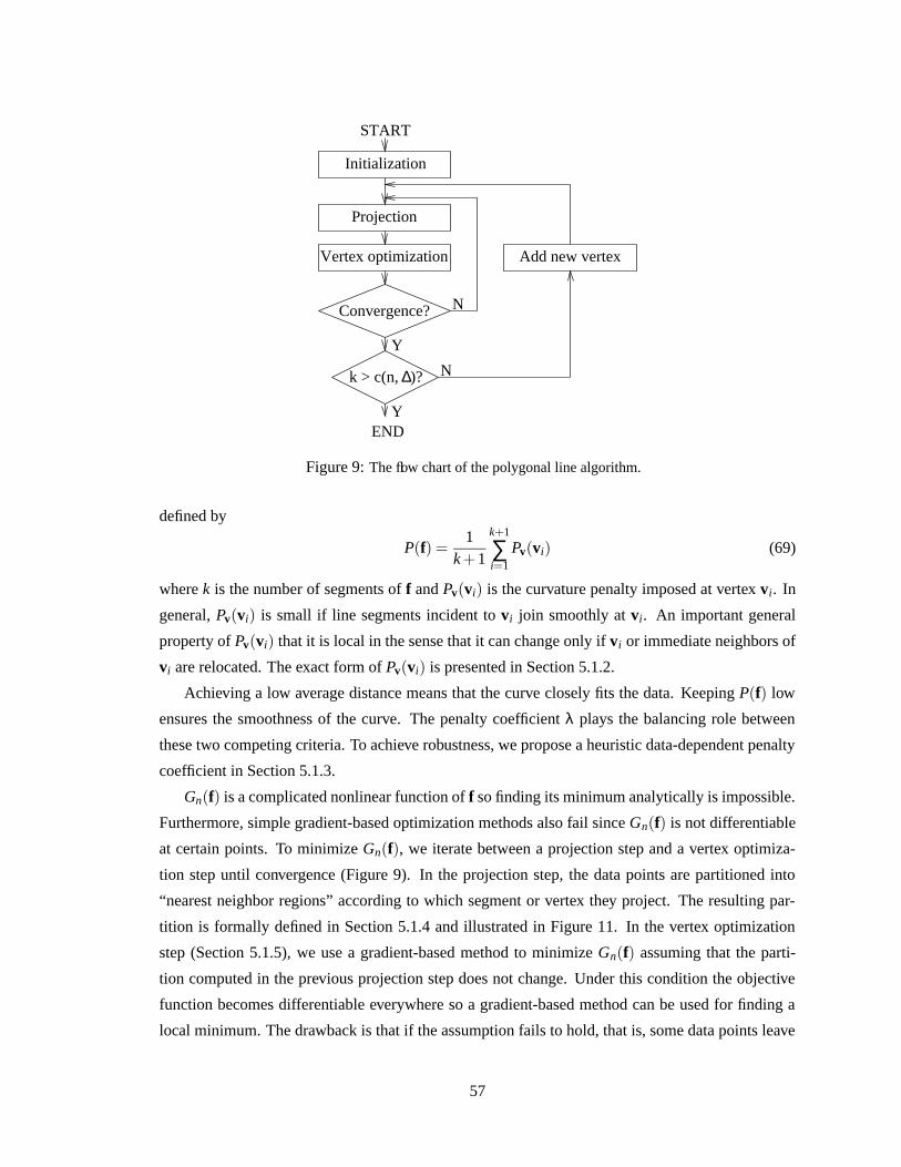
Vertex optimization

Projection

Initialization

Convergence?

∆k > c(n, )?

Add new vertex

START

END

N

Y

Y

N

Figure 9: The flow chart of the polygonal line algorithm.

defined by

P(f) =1

k +1

k+1

∑i=1

Pv(vi) (69)

where k is the number of segments of f and Pv(vi) is the curvature penalty imposed at vertex vi. In

general, Pv(vi) is small if line segments incident to vi join smoothly at vi. An important general

property of Pv(vi) that it is local in the sense that it can change only if vi or immediate neighbors of

vi are relocated. The exact form of Pv(vi) is presented in Section 5.1.2.

Achieving a low average distance means that the curve closely fits the data. Keeping P(f) low

ensures the smoothness of the curve. The penalty coefficient λ plays the balancing role between

these two competing criteria. To achieve robustness, we propose a heuristic data-dependent penalty

coefficient in Section 5.1.3.

Gn(f) is a complicated nonlinear function of f so finding its minimum analytically is impossible.

Furthermore, simple gradient-based optimization methods also fail since Gn(f) is not differentiable

at certain points. To minimize Gn(f), we iterate between a projection step and a vertex optimiza-

tion step until convergence (Figure 9). In the projection step, the data points are partitioned into

“nearest neighbor regions” according to which segment or vertex they project. The resulting par-

tition is formally defined in Section 5.1.4 and illustrated in Figure 11. In the vertex optimization

step (Section 5.1.5), we use a gradient-based method to minimize Gn(f) assuming that the parti-

tion computed in the previous projection step does not change. Under this condition the objective

function becomes differentiable everywhere so a gradient-based method can be used for finding a

local minimum. The drawback is that if the assumption fails to hold, that is, some data points leave

57

(a) (b) (c)

(d) (e) (f)

Figure 10: The curves fk,n produced by the polygonal line algorithm for n = 100 data points. The data wasgenerated by adding independent Gaussian errors to both coordinates of a point chosen randomly on a halfcircle. (a) f1,n, (b) f2,n, (c) f3,n, (d) f4,n, (e) f8,n, (f) f15,n (the output of the algorithm).

their nearest neighbor regions while vertices of the curve are moved, the objective function Gn(f)

might increase in this step. As a consequence, the convergence of the optimizing iteration cannot be

guaranteed in theory. In practice, during extensive test runs, however, the algorithm was observed

to always converge.

5.1.1 Stopping Condition

According to the theoretical results of Section 4.2, the number of segments k is an important factor

that controls the balance between the estimation and approximation errors, and it should be propor-

tional to n1/3 to achieve the O(n−1/3) convergence rate for the expected squared distance. Although

the theoretical bounds are not tight enough to determine the optimal number of segments for a given

data size, we have found that k ∼ n1/3 works in practice. We have also found that the final value

of k should also depend on the average squared distance to achieve robustness. If the variance of

the noise is relatively small, we can keep the approximation error low by allowing a relatively large

number of segments. On the other hand, when the variance of the noise is large (implying a high

58

estimation error), a low approximation error does not improve the overall performance significantly,

so in this case a smaller number of segments can be chosen. The stopping condition blends these

two considerations. The algorithm stops when k exceeds

c(

n,∆n(fk,n))

= βn1/3 r√

∆n(fk,n)(70)

where r is the “radius” of the data defined by

r = maxx∈Xn

∥

∥

∥x− 1

n ∑y∈Xn

y∥

∥

∥(71)

(included to achieve scale-independence), and β is a parameter of the algorithm which was deter-

mined by experiments and was set to the constant value 0.3.

Note that in a practical sense, the number of segments plays a more important role in determin-

ing the computational complexity of the algorithm than in measuring the quality of the approxima-

tion. Experiments showed that, due to the data-dependent curvature penalty, the number of segments

can increase even beyond the number of data points without any indication of overfitting. While in-

creasing the number of segments beyond a certain limit offers only marginal improvement in the

approximation, it causes the algorithm to slow down considerably. Therefore, in on-line applica-

tions, where speed has priority over precision, it is reasonable to use a smaller number of segments

than indicated by (70), and if “aesthetic” smoothness is an issue, to fit a spline through the vertices

of the curve (see Section 6.2.2 for an example).

5.1.2 The Curvature Penalty

The most important heuristic component of the algorithm is the curvature penalty P(vi) imposed at

a vertex vi. In the theoretical algorithm the average squared distance ∆n(x, f) is minimized subject

to the constraint that f is a polygonal line with k segments and length not exceeding L. One could

use a Lagrangian formulation and attempt to optimize f by minimizing a penalized squared error of

the form ∆n(f)+λl(f)2. Although this direct length penalty can work well in certain applications, it

yields poor results in terms of recovering a smooth generating curve. In particular, this approach is

very sensitive to the choice of λ and tends to produce curves which, similarly to the HS algorithm,

exhibit a “flattening” estimation bias towards the center of the curvature.

Instead of an explicit length penalty, to ensure smoothness of the curve, we penalize sharp

angles between line segments. At inner vertices vi, 2 ≤ i ≤ k, we penalize the cosine of the angle

of the two incident line segment of vi. The cosine function is convex in the interval [π/2,π] and

its derivative is zero at π which makes it especially suitable for the steepest descent algorithm. To

make the algorithm invariant under scaling, we multiply the cosines by the squared radius (71) of

the data. At the endpoints (vi, i = 1,k +1), we keep the direct penalty on the squared length of the

59

first (or last) segment as suggested by the theoretical model. Formally, let γi denote the angle at

vertex vi, let π(vi) = r2(1 + cosγi), let µ+(vi) = ‖vi − vi+1‖2, and let µ−(vi) = ‖vi − vi−1‖2. Then

the penalty imposed at vi is defined by

Pv(vi) =

µ+(vi) if i = 1,

π(vi) if 1 < i < k +1,

µ−(vi) if i = k +1.

(72)

Although we do not have a formal proof, we offer the following informal argument to support

our observation that the principal curve exhibits a substantially smaller estimation bias if the pro-

posed curvature penalty is used instead of a direct length penalty. When calculating the gradient of

the penalty with respect to an inner vertex vi, it is assumed that all vertices of the curve are fixed

except vi. If a direct penalty on the squared length of the curve is used, the gradient of the penalty

can be calculated as the gradient of the local length penalty at vi (1 < i < k +1) defined as

Pl(vi) = l(si−1)2 + l(si)

2 = ‖vi −vi−1‖2 +‖vi −vi+1‖2.

This local length penalty is minimized if the angle at vi is π, which means that the gradient vector

induced by the penalty always points towards the center of the curvature. If the data is spread equally

to the two sides of the generating curve, the distance term cannot balance the inward-pulling effect

of the penalty, so the estimated principal curve will always produce a bias towards the center of the

curvature. On the other hand, if we penalize sharp angles at vi and at the two immediate neighbors

of vi (the three angles that can change if vi is moved while all other vertices are fixed), the minimum

is no longer achieved at π but at a smaller angle.

Note that the chosen penalty formulation is related to the original principle of penalizing the

length of the curve. At inner vertices, penalizing sharp angles indirectly penalizes long segments.

At the endpoints (vi, i = 1,k + 1), where penalizing sharp angles does not translate to penalizing

long line segments, the penalty on a nonexistent angle is replaced by a direct penalty on the squared

length of the first (or last) segment. Also note that although the direct length penalty yields poor

results in terms of recovering a smooth generating curve, it may be used effectively under different

assumptions.

5.1.3 The Penalty Factor

One important issue is the amount of smoothing required for a given data set. In the HS algorithm

one needs to determine the penalty coefficient of the spline smoother, or the span of the scatterplot

smoother. In our algorithm, the corresponding parameter is the curvature penalty factor λ. If some

a priori knowledge about the distribution is available, one can use it to determine the smoothing

60

parameter. However, in the absence of such knowledge, the coefficient should be data-dependent.

Based on heuristic considerations explained below, and after carrying out practical experiments, we

set

λ = λ′ · k

n1/3·√

∆n(fk,n)

r(73)

where λ′ is a parameter of the algorithm which was determined by experiments and was set to the

constant value 0.13.

By setting the penalty to be proportional to the average distance of the data points from the

curve, we avoid the zig-zagging behavior of the curve resulting from overfitting when the noise is

relatively large. At the same time, this penalty factor allows the principal curve to closely follow

the generating curve when the generating curve itself is a polygonal line with sharp angles and the

data is concentrated on this curve (the noise is very small).

In our experiments we have found that the algorithm is more likely to avoid local minima if a

small penalty is imposed initially and the penalty is gradually increased as the number of segments

grows. The number of segments is normalized by n1/3 since the final number of segments, according

to the stopping condition (Section 5.1.1), is proportional to n1/3.

5.1.4 The Projection Step

Let f denote a polygonal line with vertices v1, . . . ,vk+1 and line segments s1, . . . ,sk, such that si

connects vertices vi and vi+1. In this step the data set Xn is partitioned into (at most) 2k +1 disjoint

sets V1, . . . ,Vk+1 and S1, . . . ,Sk, the nearest neighbor regions of the vertices and segments of f, re-

spectively, in the following manner. For any x ∈ Rd let ∆(x,si) be the squared distance from x to si

(see definition (21) on page 21), let ∆(x,vi) = ‖x−vi‖2, and let

Vi ={

x ∈ Xn : ∆(x,vi) = ∆(x, f), ∆(x,vi) < ∆(x,vm), m = 1, . . . , i−1}

.

Upon setting V =Sk+1

i=1 Vi, the Si sets are defined by

Si ={

x ∈ Xn : x 6∈V, ∆(x,si) = ∆(x, f),∆(x,si) < ∆(x,sm),m = 1, . . . , i−1}

.

The resulting partition is illustrated in Figure 11.

5.1.5 The Vertex Optimization Step

In this step we attempt to minimize the penalized distance function (68) assuming that none of

the data points leave the nearest neighbor cell of a line segment or a vertex. This is clearly an

incorrect assumption but without it we could not use any gradient-based minimization method since

the distance of a point x and the curve is not differentiable (with respect to the vertices of the

61

iV

Si

Si+1is

i

vv

1

Vi+1

Si-2

s

i-

2s

1

1vi+1

i-S1i-

i-

V

i+

s i-1

Figure 11: A nearest neighbor partition of R2 induced by the vertices and segments of f. The nearest point

of f to any point in the set Vi is the vertex vi. The nearest point of f to any point in the set Si is a point of theline segment si.

curve) if x falls on the boundary of two nearest neighbor regions. Also, to check whether a data

point has left the nearest neighbor cell of a line segment or a vertex, we would have to execute a

projection step each time when a vertex is moved, which is computationally infeasible. Technically,

this assumption means that the distance of a data point x and a line segment si is measured as if si

were an infinite line. Accordingly, let s′i be the line obtained by the infinite extension of the line

segment si, let

σ+(vi) = ∑x∈Si

∆(x,s′i),

σ−(vi) = ∑x∈Si−1

∆(x,s′i−1),

and

ν(vi) = ∑x∈Vi

∆(x,vi)

where ∆(x,s′i) is the Euclidean squared distance of x and the infinite line s′i as defined by (20) on

page 21, and define

∆′n(f) =

1n

(

k+1

∑i=1

ν(v)+k

∑i=1

σ+(vi)

)

.

In the vertex optimization step we minimize a “distorted” objective function G′n(f) = ∆′

n(f)+

λP(f). Note that after every projection step, until any data point crosses the boundary of a nearest

neighbor cell, the “real” distance function ∆n(f) is equal to ∆′n(f), so Gn(f) = G′

n(f).

62

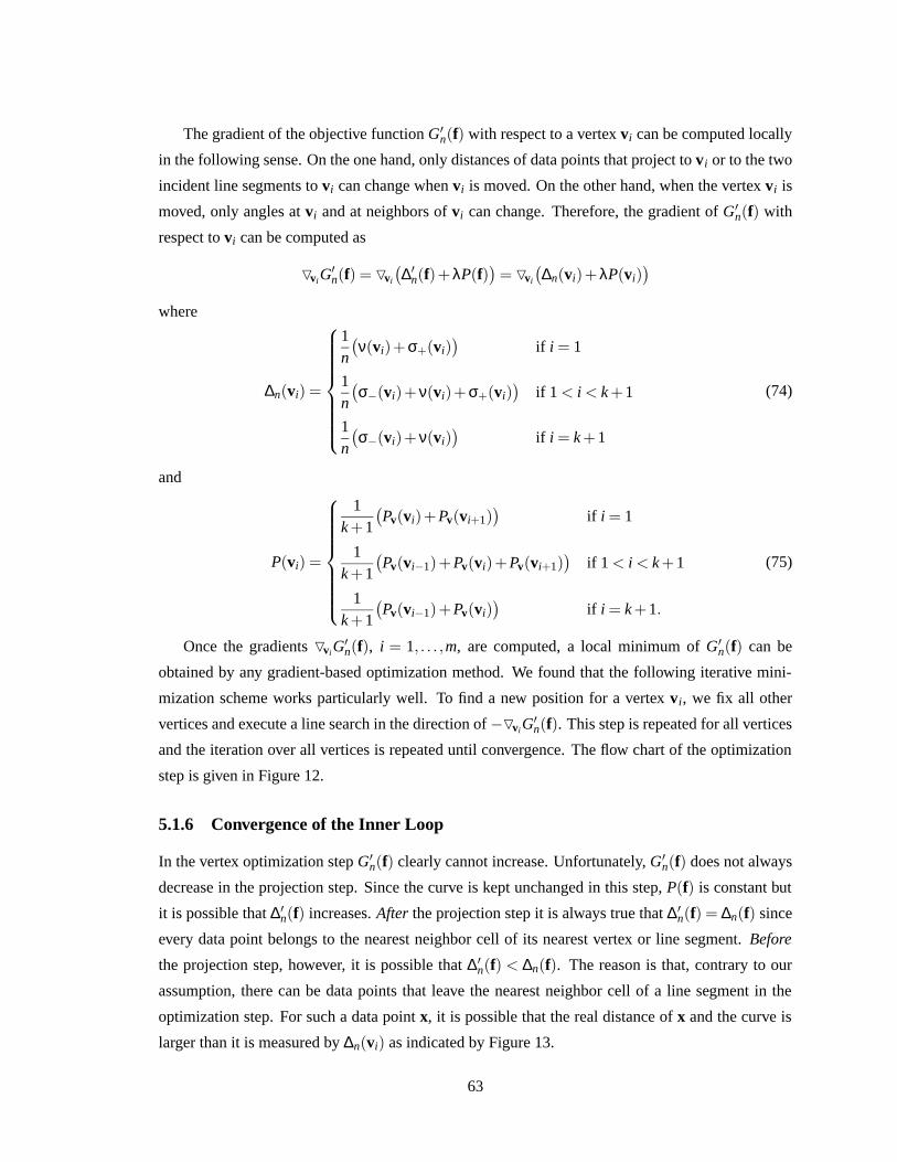
The gradient of the objective function G′n(f) with respect to a vertex vi can be computed locally

in the following sense. On the one hand, only distances of data points that project to vi or to the two

incident line segments to vi can change when vi is moved. On the other hand, when the vertex vi is

moved, only angles at vi and at neighbors of vi can change. Therefore, the gradient of G′n(f) with

respect to vi can be computed as

OviG′n(f) = Ovi

(

∆′n(f)+λP(f)

)

= Ovi

(

∆n(vi)+λP(vi))

where

∆n(vi) =

1n

(

ν(vi)+σ+(vi))

if i = 1

1n

(

σ−(vi)+ν(vi)+σ+(vi))

if 1 < i < k +1

1n

(

σ−(vi)+ν(vi))

if i = k +1

(74)

and

P(vi) =

1k +1

(

Pv(vi)+Pv(vi+1))

if i = 1

1k +1

(

Pv(vi−1)+Pv(vi)+Pv(vi+1))

if 1 < i < k +1

1k +1

(

Pv(vi−1)+Pv(vi))

if i = k +1.

(75)

Once the gradients OviG′n(f), i = 1, . . . ,m, are computed, a local minimum of G′

n(f) can be

obtained by any gradient-based optimization method. We found that the following iterative mini-

mization scheme works particularly well. To find a new position for a vertex vi, we fix all other

vertices and execute a line search in the direction of −OviG′n(f). This step is repeated for all vertices

and the iteration over all vertices is repeated until convergence. The flow chart of the optimization

step is given in Figure 12.

5.1.6 Convergence of the Inner Loop

In the vertex optimization step G′n(f) clearly cannot increase. Unfortunately, G′

n(f) does not always

decrease in the projection step. Since the curve is kept unchanged in this step, P(f) is constant but

it is possible that ∆′n(f) increases. After the projection step it is always true that ∆′

n(f) = ∆n(f) since

every data point belongs to the nearest neighbor cell of its nearest vertex or line segment. Before

the projection step, however, it is possible that ∆′n(f) < ∆n(f). The reason is that, contrary to our

assumption, there can be data points that leave the nearest neighbor cell of a line segment in the

optimization step. For such a data point x, it is possible that the real distance of x and the curve is

larger than it is measured by ∆n(vi) as indicated by Figure 13.

63

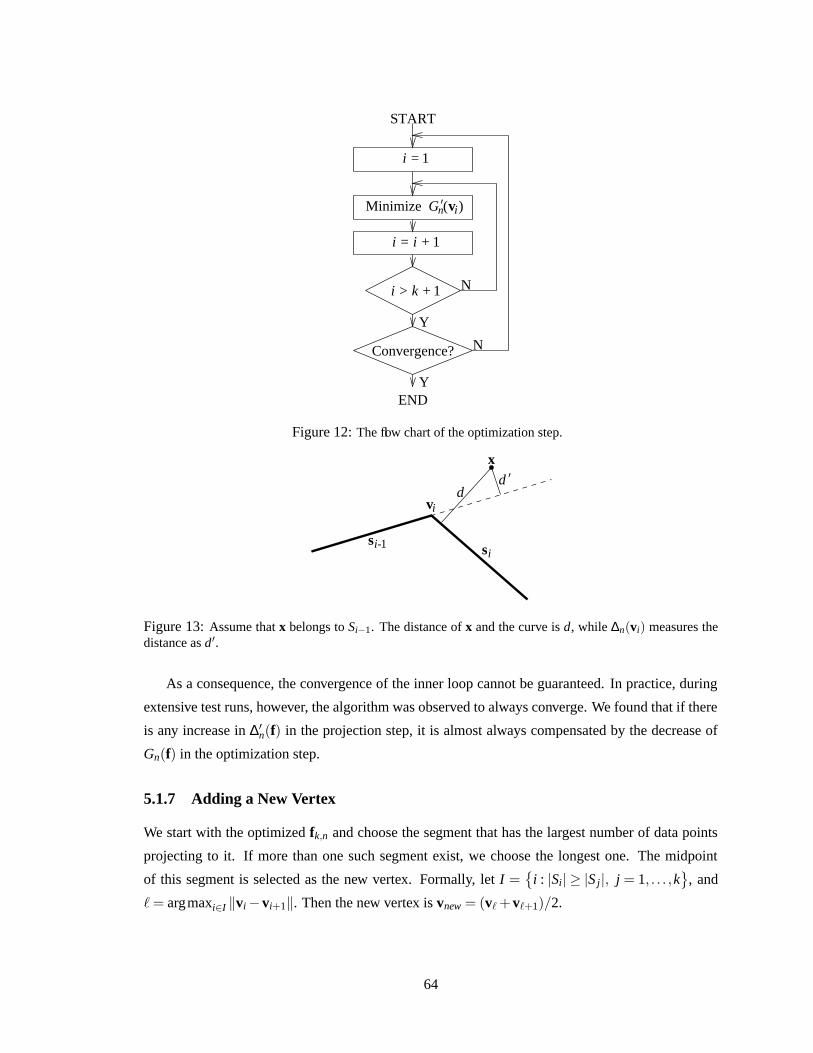
vin

1

1

G’

1

Y

N

i =

i = i +

i > k +

Convergence?

END

START

Y

Minimize ( )

N

Figure 12: The flow chart of the optimization step.

si

vi

’dd

x

si-1

Figure 13: Assume that x belongs to Si−1. The distance of x and the curve is d, while ∆n(vi) measures thedistance as d′.

As a consequence, the convergence of the inner loop cannot be guaranteed. In practice, during

extensive test runs, however, the algorithm was observed to always converge. We found that if there

is any increase in ∆′n(f) in the projection step, it is almost always compensated by the decrease of

Gn(f) in the optimization step.

5.1.7 Adding a New Vertex

We start with the optimized fk,n and choose the segment that has the largest number of data points

projecting to it. If more than one such segment exist, we choose the longest one. The midpoint

of this segment is selected as the new vertex. Formally, let I ={

i : |Si| ≥ |S j|, j = 1, . . . ,k}

, and

` = argmaxi∈I ‖vi −vi+1‖. Then the new vertex is vnew = (v` +v`+1)/2.

64

5.1.8 Computational Complexity

The complexity of the inner loop is dominated by the complexity of the projection step, which

is O(nk). Increasing the number of segments one at a time (as described in Section 5.1.7), the

complexity of the algorithm to obtain fk,n is O(nk2). Using the stopping condition of Section 5.1.1,

the computational complexity of the algorithm becomes O(n5/3). This is slightly better than the

O(n2) complexity of the HS algorithm.

The complexity can be dramatically decreased in certain situations. One possibility is to add

more than one vertex at a time. For example, if instead of adding only one vertex, a new vertex

is placed at the midpoint of every segment, then we can reduce the computational complexity for

producing fk,n to O(nk logk). One can also set k to be a constant if the data size is large, since

increasing k beyond a certain threshold brings only diminishing returns. Also, k can be naturally set

to a constant in certain applications, giving O(nk) computational complexity. These simplifications

work well in certain situations, but the original algorithm is more robust.

Note that the optimization of Gn(vi) can be done in O(1) time if the sample mean of the data

points in Vi, and the sample means and the sample covariance matrices of the data points in Si−1 and

Si are stored. The maintenance of these statistics can be done in the projection step when the data

points are sorted into the nearest neighbor sets. The statistics must be updated only for data points

that are moved from a nearest neighbor set into another in the projection step. The number of such

data points tends to be very small as the algorithm progresses so the computational requirements of

this operation is negligible compared to other steps of the algorithm.

The projection step can be accelerated by using special data structures. The construction we

present here is based on the following two observations. Firstly, when the noise is relatively low

and the line segments are relatively long, most of the data points are very far from the second nearest

line segment compared to their distance from the curve. Secondly, as the algorithm progresses, the

vertices move less and less in the optimization step so most of the data points stay in their original

nearest neighbor sets. If we can guarantee that a given data point x stays in its nearest neighbor set,

we can save the time of measuring the distance between x and each line segment of the curve.

Formally, let δv( j) be the maximum shift of a vertex in the jth optimization step defined by

δv( j) =

∞ if j = 0

maxi=1,...,k+1

∥

∥

∥v( j)

i −v( j+1)i

∥

∥

∥otherwise.

Let the distance between a data point x and a line segment s be

d(x,s) =√

∆(x,s) = ‖x− s(ts(x))‖.

First we show that the distance between any data point and any line segment can change at most

65

δv( j) in the jth optimization step. Let t1 = ts( j)(x) and t2 = ts( j+1)(x), assume that both s( j) and s( j+1)

are parameterized over [0,1], and assume that d(

x,s( j))

≥ d(

x,s( j+1))

. Then we have

∣

∣

∣d(

x,s( j))

−d(

x,s( j+1))∣

∣

∣

= d(

x,s( j))

−d(

x,s( j+1))

=∥

∥

∥x− s( j)(t1)

∥

∥

∥−∥

∥

∥x− s( j+1)(t2)

∥

∥

∥

≤∥

∥

∥x− s( j)(t2)

∥

∥

∥−∥

∥

∥x− s( j+1)(t2)

∥

∥

∥(76)

≤∥

∥

∥s( j)(t2)− s( j+1)(t2)

∥

∥

∥(77)

=∥

∥

∥t2s( j)(0)− (1− t2)s( j)(1)− t2s( j+1)(0)+(1− t2)s( j+1)(1)

∥

∥

∥

≤ t2∥

∥

∥s( j)(0)− s( j+1)(0)

∥

∥

∥+(1− t2)

∥

∥

∥s( j+1)(1)− s( j)(1)

∥

∥

∥(78)

≤ δv( j) (79)

where (76) holds because s( j)(t1) is the closest point of s( j) to x, (77) and (78) follows from the

triangle inequality, and (79) follows from the assumption that none of the endpoints of s( j) are

shifted by more than δv( j). By symmetry, a similar inequality holds if d(

x,s( j))

< d(

x,s( j+1))

.

Now consider a data point x, and let s( j)i1 and s( j)

i2 be the nearest and second nearest line segments

to x, respectively. Then if

d(

x,s( j)i1

)

≤ d(

x,s( j)i2

)

−2δv( j), (80)

then for any i 6= i1, we have

d(

x,s( j+1)i1

)

≤ d(

x,s( j)i1

)

+δv( j) (81)

≤ d(

x,s( j)i2

)

−δv( j) (82)

≤ d(

x,s( j)i

)

−δv( j) (83)

≤ d(

x,s( j+1)i

)

(84)

where (81) and (84) follows from (79), (82) follows from (80), and (83) holds since s( j)i2 is the second

nearest line segment to x. (84) means that if (80) holds, si1 remains the nearest line segment to x

after the jth optimization step. Furthermore, it is easy to see that after the ( j + j1)th optimization

step, si1 is still the nearest line segment to x if

d(

x,s( j)i1

)

≤ d(

x,s( j)i2

)

−2j+ j1

∑= j

δv(`).

Practically, this means that in the subsequent projection steps we only have to decide whether x

belongs to Si1 , Vi1 , or Vi1+1. So, by storing the index of the first and second nearest segment for each

66

data point x, and computing the maximum shift δv( j) after each optimization step, we can save a lot

of computation in the projection steps especially towards the end of the optimization when δv( j) is

relatively small.

5.1.9 Remarks

Heuristic Versus Core Components

It should be noted that the two core components of the algorithm, the projection and the vertex

optimization steps, are combined with more heuristic elements such as the stopping condition (70)

the form of the penalty term (75) of the optimization step. The heuristic parts of the algorithm have

been tailored to the task of recovering an underlying generating curve for a distribution based on

a finite data set of randomly drawn points (see the experimental results in Section 5.2). When the

algorithm is intended for an application with a different objective, the core components can be kept

unchanged but the heuristic elements may be replaced according to the new objectives.

Relationship with the SOM algorithm

As a result of introducing the nearest neighbor regions Si and Vi, the polygonal line algorithm

substantially differs from methods based on the self-organizing map (Section 3.2.2). On the one

hand, although we optimize the positions of the vertices of the curve, the distances of the data

points are measured from the line segments and vertices of the curve onto which they project, which

means that the manifold fitted to the data set is indeed a polygonal curve. On the other hand, the self-

organizing map measures distances exclusively from the vertices, and the connections serve only as

a tool to visualize the topology of the map. The line segments are not, by any means, part of the

manifold fitted to the data set. Therefore, even if the resulted map looks like a polygonal curve (as

it does if the topology is one-dimensional), the optimized manifold remains the set of codepoints,

not the depicted polygonal curve.

One important practical implication of our principle is that we can use a relatively small number

of vertices and still obtain good approximation to an underlying generating curve.

Relationship of Four Unsupervised Learning a Algorithms

There is an interesting informal relationship between the HS algorithm with spline smoothing, the

polygonal line algorithm, Tibshirani’s semi-parametric model (Section 3.2.1, [Tib92]), and the Gen-

erative Topographic Mapping (Bishop et al.’s [BSW98] principled alternative to SOM described

briefly in Section 3.2.2). On the one hand, the HS algorithm and the polygonal line algorithm

assume a nonparametric model of the source distribution whereas Tibshirani’s algorithm and the

67

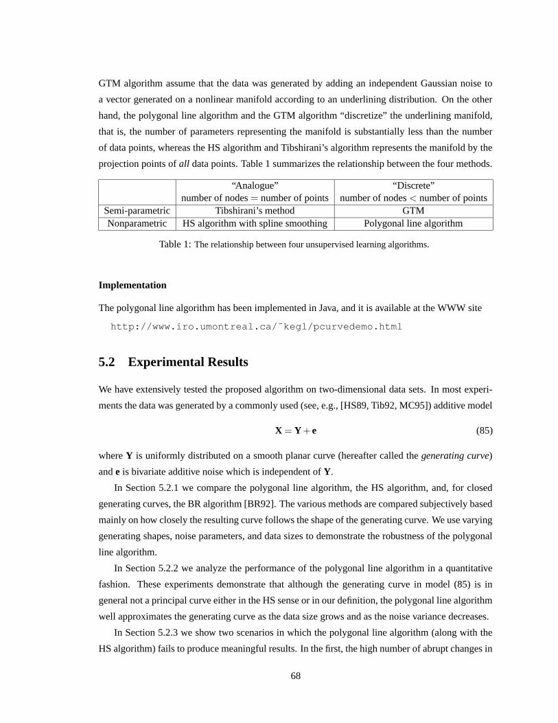
GTM algorithm assume that the data was generated by adding an independent Gaussian noise to

a vector generated on a nonlinear manifold according to an underlining distribution. On the other

hand, the polygonal line algorithm and the GTM algorithm “discretize” the underlining manifold,

that is, the number of parameters representing the manifold is substantially less than the number

of data points, whereas the HS algorithm and Tibshirani’s algorithm represents the manifold by the

projection points of all data points. Table 1 summarizes the relationship between the four methods.

“Analogue”number of nodes = number of points

“Discrete”number of nodes < number of points

Semi-parametric Tibshirani’s method GTMNonparametric HS algorithm with spline smoothing Polygonal line algorithm

Table 1: The relationship between four unsupervised learning algorithms.

Implementation

The polygonal line algorithm has been implemented in Java, and it is available at the WWW site

http://www.iro.umontreal.ca/˜kegl/pcurvedemo.html

5.2 Experimental Results

We have extensively tested the proposed algorithm on two-dimensional data sets. In most experi-

ments the data was generated by a commonly used (see, e.g., [HS89, Tib92, MC95]) additive model

X = Y+ e (85)

where Y is uniformly distributed on a smooth planar curve (hereafter called the generating curve)

and e is bivariate additive noise which is independent of Y.

In Section 5.2.1 we compare the polygonal line algorithm, the HS algorithm, and, for closed

generating curves, the BR algorithm [BR92]. The various methods are compared subjectively based

mainly on how closely the resulting curve follows the shape of the generating curve. We use varying

generating shapes, noise parameters, and data sizes to demonstrate the robustness of the polygonal

line algorithm.

In Section 5.2.2 we analyze the performance of the polygonal line algorithm in a quantitative

fashion. These experiments demonstrate that although the generating curve in model (85) is in

general not a principal curve either in the HS sense or in our definition, the polygonal line algorithm

well approximates the generating curve as the data size grows and as the noise variance decreases.

In Section 5.2.3 we show two scenarios in which the polygonal line algorithm (along with the

HS algorithm) fails to produce meaningful results. In the first, the high number of abrupt changes in

68

the direction of the generating curve causes the algorithm to oversmooth the principal curve, even

when the data is concentrated on the generating curve. This is a typical situation when the penalty

parameter λ′ should be decreased. In the second scenario, the generating curve is too complex (e.g.,

it contains loops, or it has the shape of a spiral), so the algorithm fails to find the global structure of

the data if the process is started from the first principal component. To recover the generating curve,

one must replace the initialization step by a more sophisticated routine that approximately captures

the global structure of the data.

5.2.1 Comparative Experiments

In general, in simulation examples considered by HS, the performance of the new algorithm is

comparable with the HS algorithm. Due to the data dependence of the curvature penalty factor and

the stopping condition, our algorithm turns out to be more robust to alterations in the data generating

model, as well as to changes in the parameters of the particular model.

We use model (85) with varying generating shapes, noise parameters, and data sizes to demon-

strate the robustness of the polygonal line algorithm. All plots show the generating curve, the curve

produced by our polygonal line algorithm (Polygonal principal curve), and the curve produced by

the HS algorithm with spline smoothing (HS principal curve), which we have found to perform

better than the HS algorithm using scatterplot smoothing. For closed generating curves we also

include the curve produced by the BR algorithm [BR92] (BR principal curve), which extends the

HS algorithm to closed curves. The two coefficients of the polygonal line algorithm are set in all

experiments to the constant values β = 0.3 and λ′ = 0.13.

In Figure 14 the generating curve is a circle of radius r = 1, the sample size is n = 100, and

e = (e1,e2) is a zero mean bivariate uncorrelated Gaussian with variance E(e2i ) = 0.04, for i = 1,2.

The performance of the three algorithms (HS, BR, and the polygonal line algorithm) is comparable,

although the HS algorithm exhibits more bias than the other two. Note that the BR algorithm [BR92]

has been tailored to fit closed curves and to reduce the estimation bias. In Figure 15, only half of

the circle is used as a generating curve and the other parameters remain the same. Here, too, both

the HS and our algorithm behave similarly.

When we depart from these usual settings, the polygonal line algorithm exhibits better behavior

than the HS algorithm. In Figure 16(a) the data was generated similarly to the data set of Figure 15,

and then it was linearly transformed using the matrix(

0.7 0.4−0.8 1.0

)

. In Figure 16(b) the transformation(−1.0 −1.2

1.0 −0.2

)

was used. The original data set was generated by an S-shaped generating curve, consist-

ing of two half circles of unit radii, to which the same Gaussian noise was added as in Figure 15. In

both cases the polygonal line algorithm produces curves that fit the generator curve more closely.

This is especially noticeable in Figure 16(a) where the HS principal curve fails to follow the shape

69

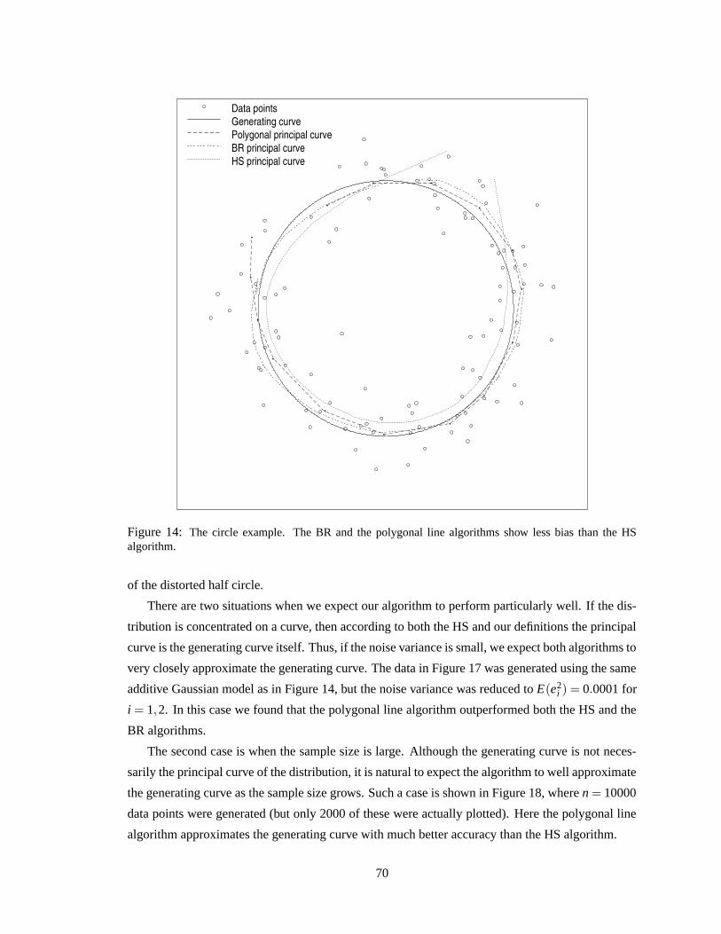
Data pointsGenerating curvePolygonal principal curveBR principal curveHS principal curve

Figure 14: The circle example. The BR and the polygonal line algorithms show less bias than the HSalgorithm.

of the distorted half circle.

There are two situations when we expect our algorithm to perform particularly well. If the dis-

tribution is concentrated on a curve, then according to both the HS and our definitions the principal

curve is the generating curve itself. Thus, if the noise variance is small, we expect both algorithms to

very closely approximate the generating curve. The data in Figure 17 was generated using the same

additive Gaussian model as in Figure 14, but the noise variance was reduced to E(e2i ) = 0.0001 for

i = 1,2. In this case we found that the polygonal line algorithm outperformed both the HS and the

BR algorithms.

The second case is when the sample size is large. Although the generating curve is not neces-

sarily the principal curve of the distribution, it is natural to expect the algorithm to well approximate

the generating curve as the sample size grows. Such a case is shown in Figure 18, where n = 10000

data points were generated (but only 2000 of these were actually plotted). Here the polygonal line

algorithm approximates the generating curve with much better accuracy than the HS algorithm.

70

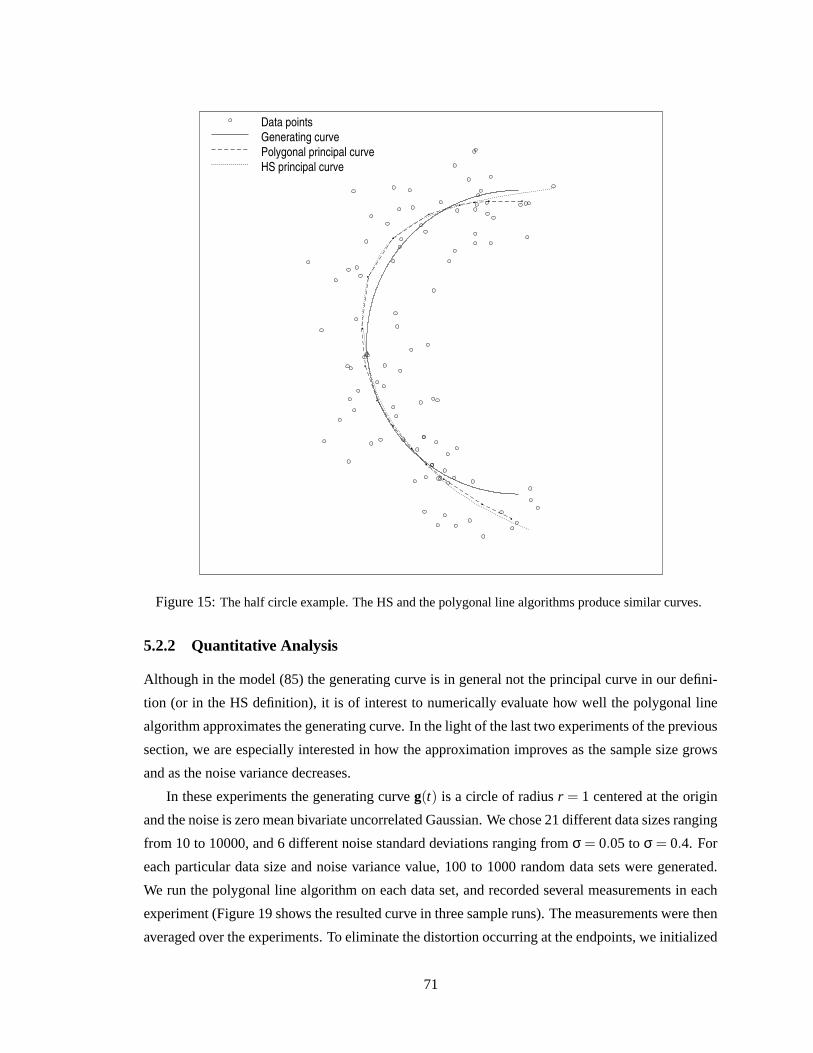
Data pointsGenerating curvePolygonal principal curveHS principal curve

Figure 15: The half circle example. The HS and the polygonal line algorithms produce similar curves.

5.2.2 Quantitative Analysis

Although in the model (85) the generating curve is in general not the principal curve in our defini-

tion (or in the HS definition), it is of interest to numerically evaluate how well the polygonal line

algorithm approximates the generating curve. In the light of the last two experiments of the previous

section, we are especially interested in how the approximation improves as the sample size grows

and as the noise variance decreases.

In these experiments the generating curve g(t) is a circle of radius r = 1 centered at the origin

and the noise is zero mean bivariate uncorrelated Gaussian. We chose 21 different data sizes ranging

from 10 to 10000, and 6 different noise standard deviations ranging from σ = 0.05 to σ = 0.4. For

each particular data size and noise variance value, 100 to 1000 random data sets were generated.

We run the polygonal line algorithm on each data set, and recorded several measurements in each

experiment (Figure 19 shows the resulted curve in three sample runs). The measurements were then

averaged over the experiments. To eliminate the distortion occurring at the endpoints, we initialized

71

(a) Distorted half circleData pointsGenerating curvePolygonal principal curveHS principal curve

(b) Distorted S-shapeData pointsGenerating curvePolygonal principal curveHS principal curve

Figure 16: Transformed data sets. The polygonal line algorithm still follows fairly closely the “distorted”shapes.

the polygonal line algorithm by a closed curve, in particular, by an equilateral triangle inscribed in

the generating circle.

For the measure of approximation, in each experiment we numerically evaluated the average

distance defined by

δ =1

l(f)

Z

mins

‖f(t)−g(s)‖dt

where the polygonal line f is parameterized by its arc length. The measurements were then aver-

aged over the experiments to obtain δn,σ for each data size n and noise standard deviation σ. The

dependence of the average distance δn,σ on the data size and the noise variance is plotted on a log-

arithmic scale in Figure 20. The resulting curves justify our informal observation made earlier that

the approximation substantially improves as the data size grows, and as the variance of the noise

decreases.

To evaluate how well the distance function of the polygonal principal curve estimates the vari-

ance of the noise, we also measured the relative difference between the standard deviation of the

noise σ and the measured RMSE(f) =√

∆n(f) defined as

ε =|σ−RMSE(f)|

σ.

The measurements were then averaged over the experiments to obtain εn,σ for each data size n and

noise standard deviation σ. The dependence of the relative error εn,σ on the data size and the noise

variance is plotted on a logarithmic scale in Figure 21. The graph indicates that, especially if the

72

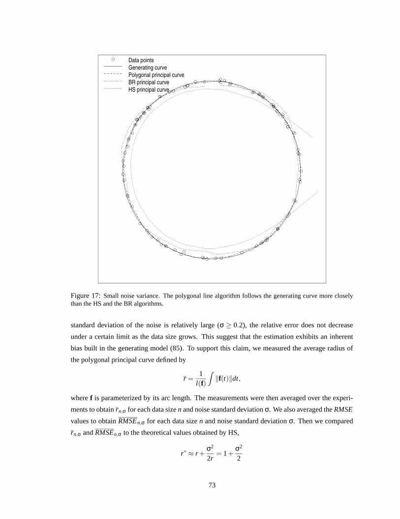
Data pointsGenerating curvePolygonal principal curveBR principal curveHS principal curve

Figure 17: Small noise variance. The polygonal line algorithm follows the generating curve more closelythan the HS and the BR algorithms.

standard deviation of the noise is relatively large (σ ≥ 0.2), the relative error does not decrease

under a certain limit as the data size grows. This suggest that the estimation exhibits an inherent

bias built in the generating model (85). To support this claim, we measured the average radius of

the polygonal principal curve defined by

r =1

l(f)

Z

‖f(t)‖dt,

where f is parameterized by its arc length. The measurements were then averaged over the experi-

ments to obtain rn,σ for each data size n and noise standard deviation σ. We also averaged the RMSE

values to obtain RMSEn,σ for each data size n and noise standard deviation σ. Then we compared

rn,σ and RMSEn,σ to the theoretical values obtained by HS,

r∗ ≈ r +σ2

2r= 1+

σ2

2

73

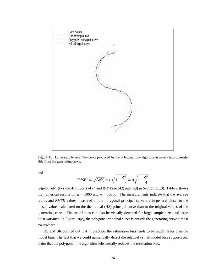
Data pointsGenerating curvePolygonal principal curveHS principal curve

Figure 18: Large sample size. The curve produced by the polygonal line algorithm is nearly indistinguish-able from the generating curve.

and

RMSE∗ =√

∆(f∗) ≈ σ

√

1− σ2

4r2 = σ

√

1− σ2

4,

respectively. (For the definitions of r∗ and ∆(f∗) see (42) and (43) in Section 3.1.3). Table 2 shows

the numerical results for n = 1000 and n = 10000. The measurements indicate that the average

radius and RMSE values measured on the polygonal principal curve are in general closer to the

biased values calculated on the theoretical (HS) principal curve than to the original values of the

generating curve. The model bias can also be visually detected for large sample sizes and large

noise variance. In Figure 19(c), the polygonal principal curve is outside the generating curve almost

everywhere.

HS and BR pointed out that in practice, the estimation bias tends to be much larger than the

model bias. The fact that we could numerically detect the relatively small model bias supports our

claim that the polygonal line algorithm substantially reduces the estimation bias.

74

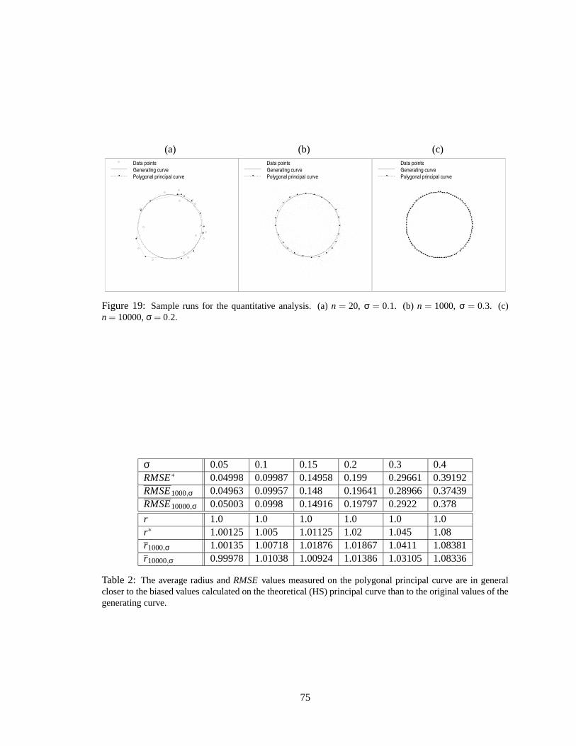
(a)Data pointsGenerating curvePolygonal principal curve

(b)Data pointsGenerating curvePolygonal principal curve

(c)Data pointsGenerating curvePolygonal principal curve

Figure 19: Sample runs for the quantitative analysis. (a) n = 20, σ = 0.1. (b) n = 1000, σ = 0.3. (c)n = 10000, σ = 0.2.

σ 0.05 0.1 0.15 0.2 0.3 0.4RMSE∗ 0.04998 0.09987 0.14958 0.199 0.29661 0.39192RMSE1000,σ 0.04963 0.09957 0.148 0.19641 0.28966 0.37439RMSE10000,σ 0.05003 0.0998 0.14916 0.19797 0.2922 0.378

r 1.0 1.0 1.0 1.0 1.0 1.0r∗ 1.00125 1.005 1.01125 1.02 1.045 1.08r1000,σ 1.00135 1.00718 1.01876 1.01867 1.0411 1.08381r10000,σ 0.99978 1.01038 1.00924 1.01386 1.03105 1.08336

Table 2: The average radius and RMSE values measured on the polygonal principal curve are in generalcloser to the biased values calculated on the theoretical (HS) principal curve than to the original values of thegenerating curve.

75

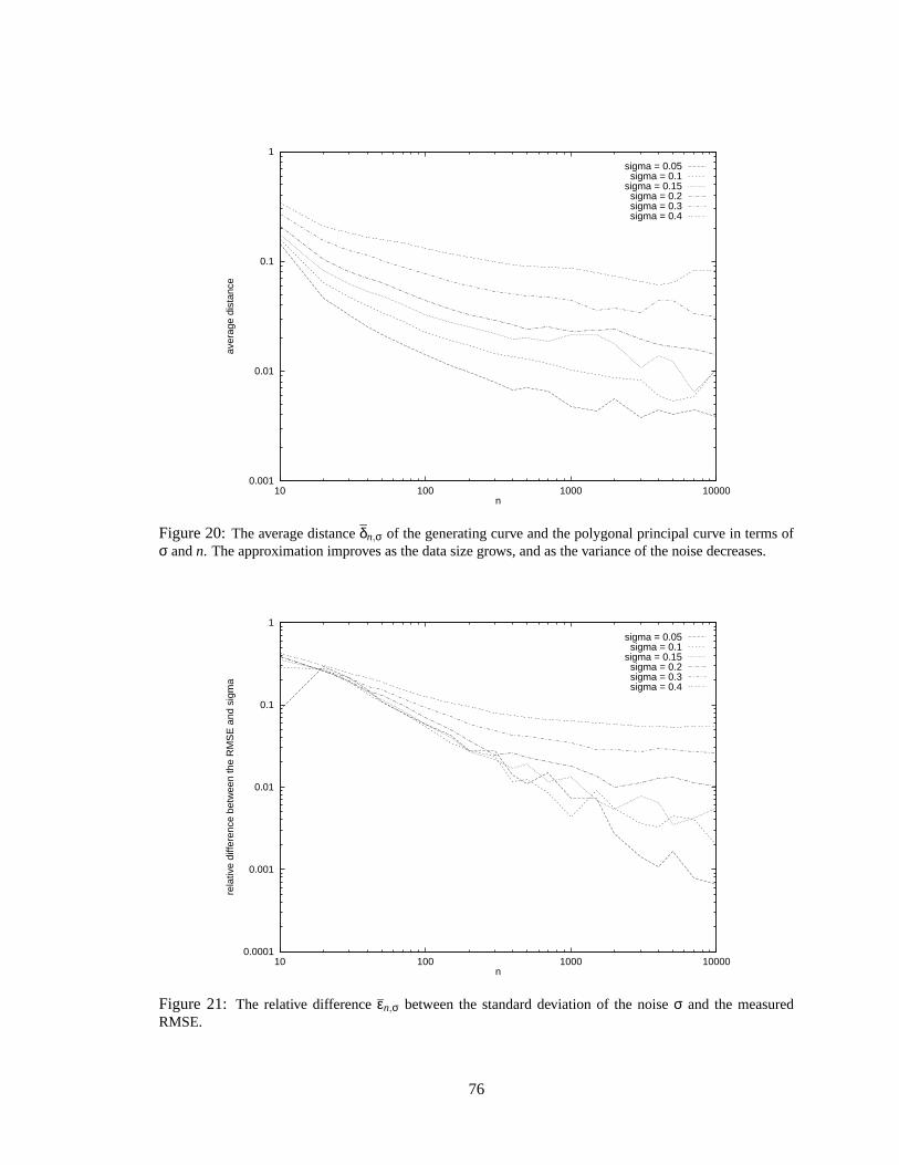
0.001

0.01

0.1

1

10 100 1000 10000

aver

age

dist

ance

n

sigma = 0.05sigma = 0.1

sigma = 0.15sigma = 0.2sigma = 0.3sigma = 0.4

Figure 20: The average distance δn,σ of the generating curve and the polygonal principal curve in terms ofσ and n. The approximation improves as the data size grows, and as the variance of the noise decreases.

0.0001

0.001

0.01

0.1

1

10 100 1000 10000

rela

tive

diffe

renc

e be

twee

n th

e R

MS

E a

nd s

igm

a

n

sigma = 0.05sigma = 0.1

sigma = 0.15sigma = 0.2sigma = 0.3sigma = 0.4

Figure 21: The relative difference εn,σ between the standard deviation of the noise σ and the measuredRMSE.

76

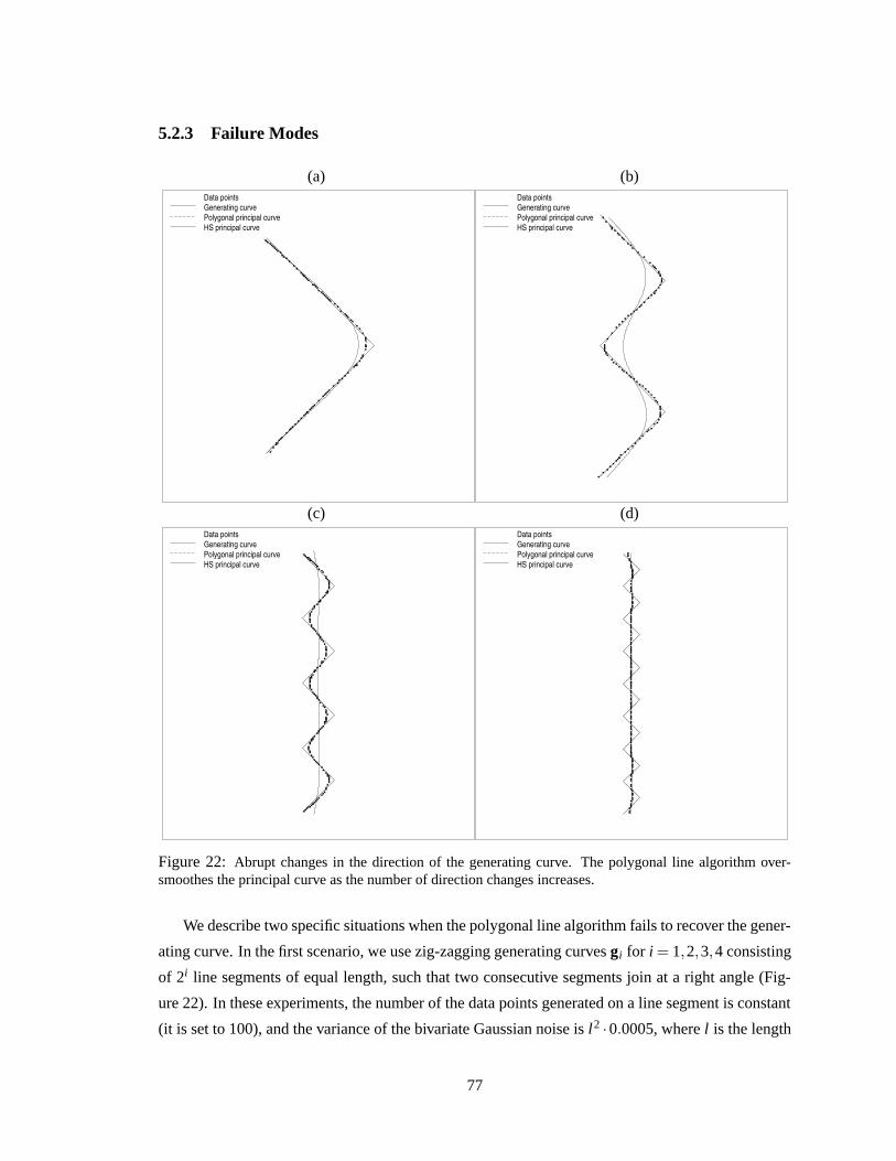
5.2.3 Failure Modes

(a)Data pointsGenerating curvePolygonal principal curveHS principal curve

(b)Data pointsGenerating curvePolygonal principal curveHS principal curve

(c)Data pointsGenerating curvePolygonal principal curveHS principal curve

(d)Data pointsGenerating curvePolygonal principal curveHS principal curve

Figure 22: Abrupt changes in the direction of the generating curve. The polygonal line algorithm over-smoothes the principal curve as the number of direction changes increases.

We describe two specific situations when the polygonal line algorithm fails to recover the gener-

ating curve. In the first scenario, we use zig-zagging generating curves gi for i = 1,2,3,4 consisting

of 2i line segments of equal length, such that two consecutive segments join at a right angle (Fig-

ure 22). In these experiments, the number of the data points generated on a line segment is constant

(it is set to 100), and the variance of the bivariate Gaussian noise is l2 ·0.0005, where l is the length

77

of a line segment. Figure 22 shows the principal curves produced by the HS and the polygonal line

algorithms in the four experiments. Although the polygonal principal curve follows the generating

curve more closely than the HS principal curve in the first three experiments (Figures 22(a), (b),

and (c)), the two algorithms produce equally poor results if the number of line segments exceeds a

certain limit (Figure 22(d)).

Analysis of the data-dependent penalty term explains this behavior of the polygonal line al-

gorithm. Since the penalty factor λp is proportional to the number of line segments, the penalty

relatively increases as the number of line segments of the generating curve grows. To achieve the

same local smoothness in the four experiments, the penalty factor should be gradually decreased as

the number of line segments of the generating curve grows. Indeed, if the constant of the penalty

term is reset to λ′ = 0.02 in the fourth experiment, the polygonal principal curve recovers the gen-

erating curve with high accuracy (Figure 23).

Data pointsGenerating curvePolygonal principal curve

Figure 23: The polygonal principal curve follows the zig-zagging generating curve closely if the penaltycoefficient is decreased.

The second scenario when the polygonal line algorithm fails to produce a meaningful result is

78

when the generating curve is too complex so the algorithm does not find the global structure of

the data. To test the gradual degradation of the algorithm, we used spiral-shaped generating curves

of increasing length, i.e., we set gi(t) = (t sin(iπt), t cos(iπt)) for t ∈ [0,1] and i = 1, . . . ,6. The

variance of the noise was set to 0.0001, and we generated 1000 data points in each experiment.

Figure 24 shows the principal curves produced by the HS and the polygonal line algorithms in four

experiments (i = 2,3,4,6). In the first three experiments (Figures 24(a), (b), and (c)), the polygo-

nal principal curve is almost indistinguishable from the generating curve, while the HS algorithm

either oversmoothes the principal curve (Figure 24(a) and (b)), or fails to recover the shape of the

generating curve (Figure 24(c)). In the fourth experiment both algorithms fail to find the shape of

the generating curve (Figure 24(d)). The failure here is due to the fact that the algorithm is stuck in

a local minima between the initial curve (the first principal component line) and the desired solution

(the generating curve). If this is likely to occur in an application, the initialization step must be re-

placed by a more sophisticated routine that approximately captures the global structure of the data.

Figure 25 indicates that this indeed works. Here we manually initialize both algorithms by a polyg-

onal line with eight vertices. Using this “hint”, the polygonal line algorithm produces an almost

perfect solution, while the HS algorithm still cannot recover the shape of the generating curve.

79

(a)Data pointsGenerating curvePolygonal principal curveHS principal curve

(b)Data pointsGenerating curvePolygonal principal curveHS principal curve

(c)Data pointsGenerating curvePolygonal principal curveHS principal curve

(d)Data pointsGenerating curvePolygonal principal curveHS principal curve

Figure 24: Spiral-shaped generating curves. The polygonal line algorithm fails to find the generating curveas the length of the spiral is increased.

80

Data pointsGenerating curve

Polygonal principal curveInitial curve

HS principal curve

Figure 25: The performance of the polygonal line algorithm improves significantly if the global structure ofthe generating curve is captured in the initialization step.

81

Chapter 6

Application of Principal Curves to

Hand-Written Character

Skeletonization

The main subject of this chapter is an application of an extended version of the polygonal line

algorithm to hand-written character skeletonization. Skeletonization is one of the important areas

in image processing. It is most often, although not exclusively, used for images of hand-written or

printed characters so we describe it here in this context. When we look at the image of a letter, we

see it as a collection of curves rather than a raster of pixels. Since the earliest days of computers, it

has been one of the challenges for researchers working in the area of pattern recognition to imitate

this ability of the human mind [Din55, KCRU57]. Approaching skeletonization from a practical

point of view, representing a character by a set of thin curves rather than by a raster of pixels is

useful for reducing the storage space and processing time of the character image. It was found that

this representation is particularly effective in finding relevant features of the character for optical

character recognition [Deu68, AH69].

The objective of skeletonization is to find the medial axis of a character. Ideally, the medial axis

is defined as a smooth curve (or set of curves) that follows the shape of a character equidistantly

from its contours. In case of hand-written characters, one can also define the medial axis as the

trajectory of the penstroke that created the letter. Most skeletonization algorithms approximate the

medial axis by a unit-width binary image obtained from the original character by iteratively peeling

its contour pixels until there remains no more removable pixel [Pav80, NS84, SA86]. The process

is called the thinning of the character template, and the result is the skeleton of the character. The

different thinning methods are characterized by the rules that govern the deletion of black pixels.

In this chapter we propose another approach to skeletonization. The development of the method

82

was inspired by the apparent similarity between the definition of principal curves and the medial

axis. A principal curve is a smooth curve that goes through the “middle” of a data set, whereas

the medial axis is a set of smooth curves that go equidistantly from the contours of a character.

Therefore, by representing the black pixels of a character by a two-dimensional data set, one can

use the principal curve of the data set to approximate the medial axis of the character. Other methods

using this “analogue” approach for skeletonization are described in Section 6.1. In this section we

also summarize existing applications of the HS principal curve algorithm.

Since the medial axis can be a set of connected curves rather then only one curve, in Section 6.2

we extend the polygonal line algorithm to find a principal graph of a data set. The extended algo-

rithm also contains two elements specific to the task of skeletonization, an initialization method to

capture the approximate topology of the character, and a collection of restructuring operations to

improve the structural quality of the skeleton produced by the initialization method. To avoid con-

fusion, in what follows we use the term skeleton for the unit-width binary image approximating the

medial axis, and we refer to the set of connected curves produced by the polygonal line algorithm

as the skeleton graph of the character template.

In Section 6.3 test results of the extended polygonal line algorithm are presented. In Sec-

tion 6.3.1 we apply the algorithm to isolated hand-written digits from the NIST Special Database

19 [Gro95]. The results indicate that the proposed algorithm finds a smooth medial axis of the great

majority of a wide variety of character templates, and substantially improves the pixelwise skele-

ton obtained by traditional thinning methods. In Section 6.3.2 we present results of experiments

with images of continuous handwriting. These experiments demonstrate that the skeleton graph

produced by the algorithm can be used for representing hand-written text efficiently.

6.1 Related Work

6.1.1 Applications and Extensions of the HS Algorithm

Hastie [Has84] presented several experiments on real data. In the first example, computer chip

waste is sampled and analyzed by two laboratories to estimate the gold content of the lot. It is in the

interest of the owner of the lot to know which laboratory produces on average lower gold content

estimates for a given sample. The principal curve method was used to point out that at higher levels

of gold content one of the laboratories produced higher assays than the other. The difference was

reversed at lower levels. [Has84] argues that these results could not have been obtained by using

standard regression techniques. In another example, a principal curve was used for non-linear factor

analysis on a data set of three-dimensional points representing measurements of mineral content of

core samples.

83

The first real application of principal curves was part of the Stanford Linear Collider project

[HS89]. The collider consists of a linear accelerator used to accelerate two particle beams, and two

arcs that bend these beams to bring them to collision. The particle beams are guided by roughly 475

magnets that lie on a smooth curve with a circumference of about three kilometers. Measurement

errors in the range of ±1 millimeters in placing the magnets resulted that the beam could not be

adequately focused. Engineers realized that it was not necessary to move the magnets to the ideal

curve, but rather to a curve through the existing positions that was smooth enough to allow focused

bending of the beam. The HS principal curve procedure was used to find this curve.

Banfield and Raftery [BR92] described an almost fully automatic method for identifying ice

floes and their outlines in satellite images. The core procedure of the method uses a closed principal

curve to estimate the floe outlines. Besides eliminating the estimation bias of the HS algorithm (see

Section 3.1.3), [BR92] also replaced the initialization step of the HS algorithm by a more sophis-

ticated routine that produced a rough estimate of the floe outlines. Furthermore, [BR92] extended

existing clustering methods by allowing groups of data points to be centered about principal curves

rather than points or lines.

Principal curve clustering was further extended and analyzed by Stanford and Raftery [SR00].

Here, fitting a principal curve is combined with the Classification EM algorithm [CG92] to itera-

tively refine clusters of data centered about principal curves. The number of clusters and the smooth-

ness parameters of the principal curves are chosen automatically by comparing approximate Bayes

factors [KR95] of different models. Combining the clustering algorithm with a denoising procedure

and an initialization procedure, [SR00] proposed an automatic method for extracting curvilinear

features of simulated and real data.

Chang and Ghosh [CG98b, CG98a] used principal curves for nonlinear feature extraction and

pattern classification. [CG98b] pointed out experimentally that a combination of the HS and BR

algorithms (the BR algorithm is run after the HS algorithm) reduces the estimation bias of the HS

algorithm and also decreases the variance of the BR algorithm that was demonstrated in Section 5.2.

[CG98b] and [CG98a] demonstrated on several examples that the improved algorithm can be used

effectively for feature extraction and classification.

Reinhard and Niranjan [RN98] applied principal curves to model the short time spectrum of

speech signals. First, high-dimensional data points representing diphones (pairs of consecutive

phones) are projected to a two-dimensional subspace. Each diphone is than modeled by a principal

curve. In the recognition phase, test data is compared to the principal curves representing the dif-

ferent diphones, and classified as the diphone represented by the nearest principal curve. [RN98]

demonstrated in experiments that the diphone recognition accuracy of can can be comparable to the

accuracy of the state-of-the-art hidden Markov models.

84

6.1.2 Piecewise Linear Approach to Skeletonization

[SWP98] used the HS principal curve algorithm for character skeletonization. The initial curve is

produced by a variant of the SOM algorithm where the neighborhood relationships are defined by

a minimum spanning tree of the pixels of the character template. The HS algorithm is then used to

fit the curve to the character template. In the expectation step a weighted kernel smoother is used

which, in this case, is equivalent to the update rule of the SOM algorithm. [SWP98] demonstrated

that principal curves can be successfully used for skeletonizing characters in fading or noisy texts

where traditional skeletonization techniques are either inapplicable or perform poorly.

Similar skeletonization methods were proposed by Mahmoud et al. [MAG91] and Datta and

Parui [DP97]. Similarly to [SWP98], [DP97] uses the SOM algorithm to optimize the positions of

vertices of a piecewise linear skeleton. The algorithm follows a “bottom-up” strategy in building

the skeletal structure: the approximation starts from a linear topology and later adds forks and loops

to the skeleton based on local geometric patterns formed during the SOM optimization. [MAG91]

proposed an algorithm to obtain piecewise linear skeletons of Arabic characters. The method is

based on fuzzy clustering and the fuzzy ISODATA algorithm [BD75] that uses a similar optimization

to the batch version of the SOM algorithm.

Although, similarly to the principal graph algorithm, [MAG91, DP97, SWP98] also use a piece-

wise linear approximation of the skeleton of the character, their approaches substantially differ from

our approach in that smoothness of the skeleton is not a primary issue in these works. Although the

SOM algorithm implicitly ensures smoothness of the skeleton to a certain extent, it lacks a clear

and intuitive formulation of the two competing criteria, smoothness of the skeleton and closeness

of the fit, which is explicitly present in our method. In this sense our algorithm complements these

methods rather then competes with them. For example, the method of [SWP98] could be used

as an alternative initialization step for the principal graph algorithm if the input is too noisy for

our thinning-based initialization step. One could also use the restructuring operations described in

[DP97] combined with the fitting-and-smoothing optimization step of the principal graph algorithm

in a “bottom-up” approach of building the skeleton graph.

6.2 The Principal Graph Algorithm

In this section we describe the principal graph algorithm, an extension of the polygonal line al-

gorithm for finding smooth skeletons of hand-written character templates. To transform binary

(black-and-white) character templates into two-dimensional data sets, we place the midpoint of the

bottom-most left-most pixel of the template to the center of a coordinate system. The unit length

of the coordinate system is set to the width (and height) of a pixel, so the midpoint of each pixel

85

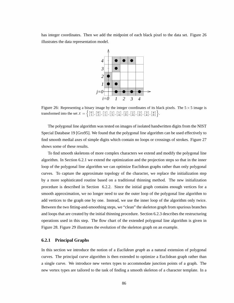
has integer coordinates. Then we add the midpoint of each black pixel to the data set. Figure 26

illustrates the data representation model.

��

4321i=0

4

3

2

1

��

j=0

Figure 26: Representing a binary image by the integer coordinates of its black pixels. The 5× 5 image is

transformed into the set X ={

[

01

]

,[

02

]

,[

11

]

,[

13

]

,[

14

]

,[

20

]

,[

24

]

,[

30

]

,[

34

]

,[

40

]

}

.

The polygonal line algorithm was tested on images of isolated handwritten digits from the NIST

Special Database 19 [Gro95]. We found that the polygonal line algorithm can be used effectively to

find smooth medial axes of simple digits which contain no loops or crossings of strokes. Figure 27

shows some of these results.

To find smooth skeletons of more complex characters we extend and modify the polygonal line

algorithm. In Section 6.2.1 we extend the optimization and the projection steps so that in the inner

loop of the polygonal line algorithm we can optimize Euclidean graphs rather than only polygonal

curves. To capture the approximate topology of the character, we replace the initialization step

by a more sophisticated routine based on a traditional thinning method. The new initialization

procedure is described in Section 6.2.2. Since the initial graph contains enough vertices for a

smooth approximation, we no longer need to use the outer loop of the polygonal line algorithm to

add vertices to the graph one by one. Instead, we use the inner loop of the algorithm only twice.

Between the two fitting-and-smoothing steps, we “clean” the skeleton graph from spurious branches

and loops that are created by the initial thinning procedure. Section 6.2.3 describes the restructuring

operations used in this step. The flow chart of the extended polygonal line algorithm is given in

Figure 28. Figure 29 illustrates the evolution of the skeleton graph on an example.

6.2.1 Principal Graphs

In this section we introduce the notion of a Euclidean graph as a natural extension of polygonal

curves. The principal curve algorithm is then extended to optimize a Euclidean graph rather than

a single curve. We introduce new vertex types to accommodate junction points of a graph. The

new vertex types are tailored to the task of finding a smooth skeleton of a character template. In a

86

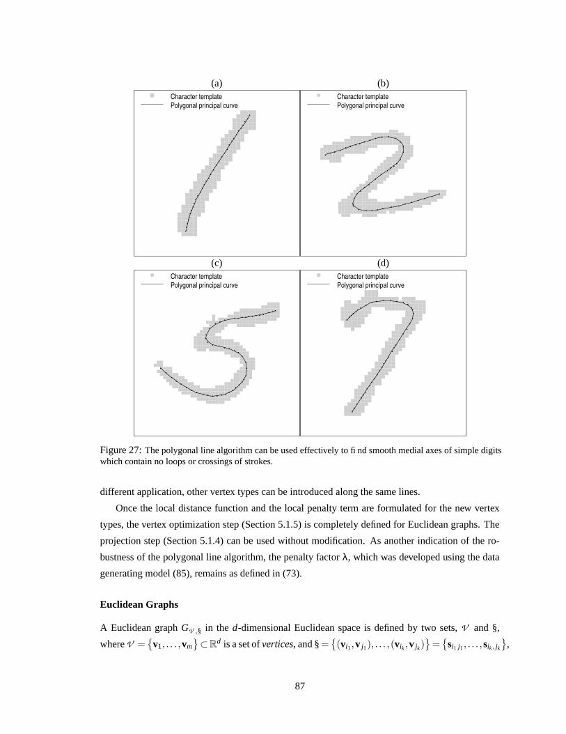
(a)Character templatePolygonal principal curve

(b)Character templatePolygonal principal curve

(c)Character templatePolygonal principal curve

(d)Character templatePolygonal principal curve

Figure 27: The polygonal line algorithm can be used effectively to find smooth medial axes of simple digitswhich contain no loops or crossings of strokes.

different application, other vertex types can be introduced along the same lines.

Once the local distance function and the local penalty term are formulated for the new vertex

types, the vertex optimization step (Section 5.1.5) is completely defined for Euclidean graphs. The

projection step (Section 5.1.4) can be used without modification. As another indication of the ro-

bustness of the polygonal line algorithm, the penalty factor λ, which was developed using the data

generating model (85), remains as defined in (73).

Euclidean Graphs

A Euclidean graph GV ,§ in the d-dimensional Euclidean space is defined by two sets, V and §,

where V ={

v1, . . . ,vm}

⊂Rd is a set of vertices, and § =

{

(vi1 ,v j1), . . . ,(vik ,v jk)}

={

si1 j1 , . . . ,sik, jk

}

,

87

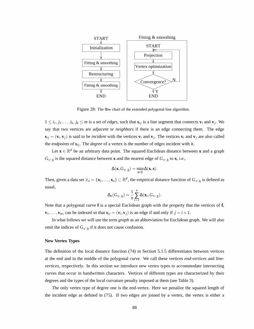
Fitting & smoothing

Vertex optimization

Projection

Convergence?

START

END

Initialization

Restructuring

Fitting & smoothingN

YEND

START

Fitting & smoothing

Figure 28: The flow chart of the extended polygonal line algorithm.

1 ≤ i1, j1, . . . , ik, jk ≤ m is a set of edges, such that si j is a line segment that connects vi and v j. We

say that two vertices are adjacent or neighbors if there is an edge connecting them. The edge

si j = (vi,v j) is said to be incident with the vertices vi and v j. The vertices vi and v j are also called

the endpoints of si j. The degree of a vertex is the number of edges incident with it.

Let x ∈ Rd be an arbitrary data point. The squared Euclidean distance between x and a graph

GV ,§ is the squared distance between x and the nearest edge of GV ,§ to x, i.e.,

∆(x,GV ,§) = mins∈§

∆(x,s).

Then, given a data set Xn = {x1, . . . ,xn} ⊂ Rd , the empirical distance function of GV ,§ is defined as

usual,

∆n(GV ,§) =1n

n

∑i=1

∆(xi,GV ,§).

Note that a polygonal curve f is a special Euclidean graph with the property that the vertices of f,

v1, . . . ,vm, can be indexed so that si j = (vi,v j) is an edge if and only if j = i+1.

In what follows we will use the term graph as an abbreviation for Euclidean graph. We will also

omit the indices of GV ,§ if it does not cause confusion.

New Vertex Types

The definition of the local distance function (74) in Section 5.1.5 differentiates between vertices

at the end and in the middle of the polygonal curve. We call these vertices end-vertices and line-

vertices, respectively. In this section we introduce new vertex types to accommodate intersecting

curves that occur in handwritten characters. Vertices of different types are characterized by their

degrees and the types of the local curvature penalty imposed at them (see Table 3).

The only vertex type of degree one is the end-vertex. Here we penalize the squared length of

the incident edge as defined in (75). If two edges are joined by a vertex, the vertex is either a

88

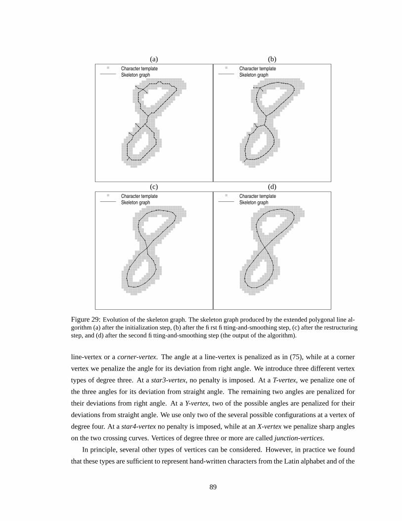
(a)Character templateSkeleton graph

(b)Character templateSkeleton graph

(c)Character templateSkeleton graph

(d)Character templateSkeleton graph

Figure 29: Evolution of the skeleton graph. The skeleton graph produced by the extended polygonal line al-gorithm (a) after the initialization step, (b) after the first fitting-and-smoothing step, (c) after the restructuringstep, and (d) after the second fitting-and-smoothing step (the output of the algorithm).

line-vertex or a corner-vertex. The angle at a line-vertex is penalized as in (75), while at a corner

vertex we penalize the angle for its deviation from right angle. We introduce three different vertex

types of degree three. At a star3-vertex, no penalty is imposed. At a T-vertex, we penalize one of

the three angles for its deviation from straight angle. The remaining two angles are penalized for

their deviations from right angle. At a Y-vertex, two of the possible angles are penalized for their

deviations from straight angle. We use only two of the several possible configurations at a vertex of

degree four. At a star4-vertex no penalty is imposed, while at an X-vertex we penalize sharp angles

on the two crossing curves. Vertices of degree three or more are called junction-vertices.

In principle, several other types of vertices can be considered. However, in practice we found

that these types are sufficient to represent hand-written characters from the Latin alphabet and of the

89

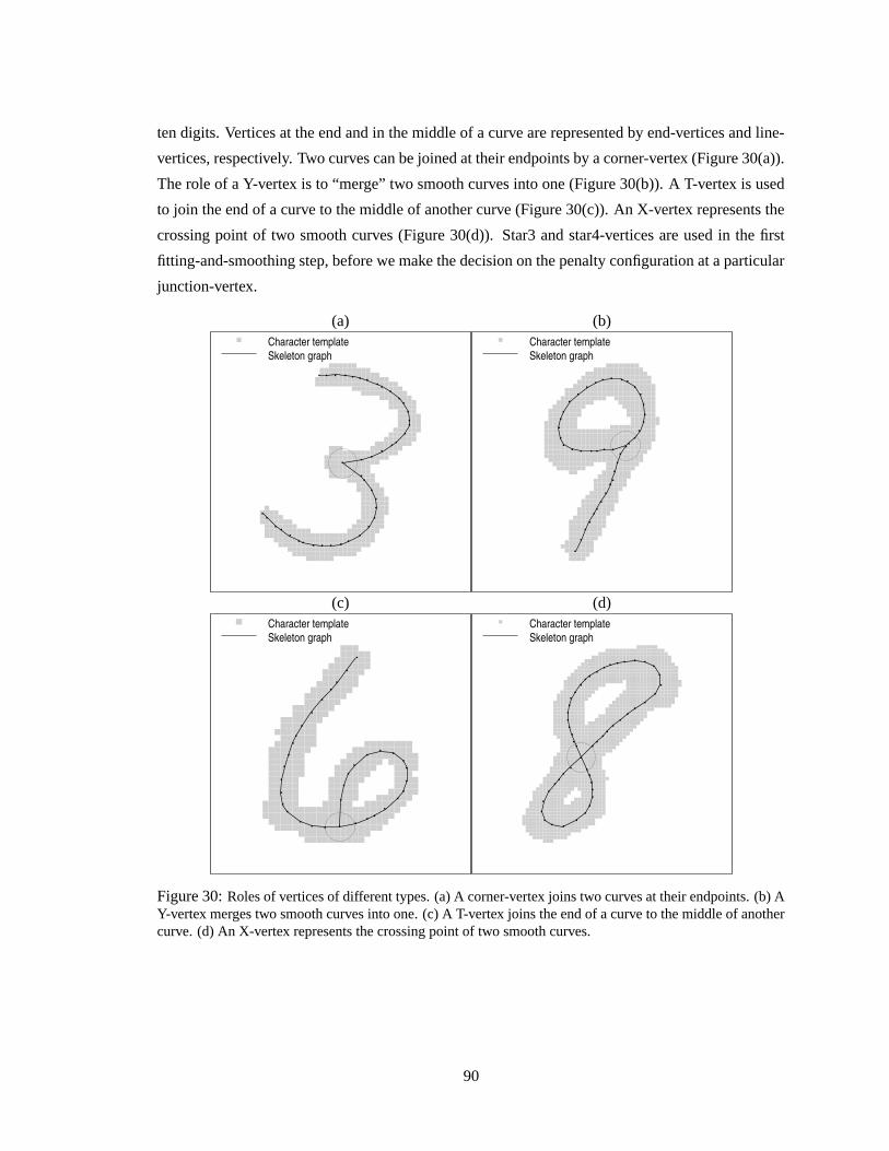
ten digits. Vertices at the end and in the middle of a curve are represented by end-vertices and line-

vertices, respectively. Two curves can be joined at their endpoints by a corner-vertex (Figure 30(a)).

The role of a Y-vertex is to “merge” two smooth curves into one (Figure 30(b)). A T-vertex is used

to join the end of a curve to the middle of another curve (Figure 30(c)). An X-vertex represents the

crossing point of two smooth curves (Figure 30(d)). Star3 and star4-vertices are used in the first

fitting-and-smoothing step, before we make the decision on the penalty configuration at a particular

junction-vertex.




(d)Character templateSkeleton graph

Figure 30: Roles of vertices of different types. (a) A corner-vertex joins two curves at their endpoints. (b) AY-vertex merges two smooth curves into one. (c) A T-vertex joins the end of a curve to the middle of anothercurve. (d) An X-vertex represents the crossing point of two smooth curves.

90

The Local Distance Function

Since the edges can no longer be naturally ordered as in the case of curves, we revise our notation

used in Chapter 5 in the formal definition of the formulas of the local distance function and the

local penalty. Let v1, . . .vm denote the vertices of the graph and let si j denote the edge that connects

vertices vi and v j. Let Vi and Si j be the nearest neighbor sets of vertex vi and edge si j, respectively,

as defined in Section 5.1.4, let s′i j be the line obtained by the infinite extension of the line segment

si j, and let

σ(si j) = ∑x∈Si j

∆(x,s′i j),

ν(vi) = ∑x∈Vi

∆(x,vi).

(Note that the new notation is a simple generalization of the notation used in Section 5.1.5 as ν(vi)

is the same as before, σ+(vi) = σ(si,i+1), and σ−(vi) = σ(si,i−1).) Then the local distance function

of vi is defined by

∆n(vi) =1n

(

ν(vi)+φi

∑j=1

σ(si,i j)

)

(86)

where φi is the degree of vi (1 ≤ φi ≤ 4), and i1, . . . , iφi are the indices of the adjacent vertices to vi.

Note that (86) is an extension of (74) where ∆n(vi) is defined for φi = 1,2.

The Local Penalty

For the definition of the local penalty, let πi j` = r2(1+ cosγi j`) be the angle penalty at v j where γi j`

denotes the angle of line segments s ji and s j`, and let µi j = ‖vi −v j‖2 be the length penalty at edge

si j. At corner and T-vertices we introduce ωi j` = 2r2 cos2 γi j` to penalize the deviation of γi j` from

right angle. The penalty Pv(vi) at vertex vi is defined in Table 3 for the different vertex types. (Note

that for end and line-vertices, Pv(vi) remains as defined in (72).) When the vertex vi is moved, only

angles at vi and at neighbors of vi can change. Therefore, the total penalty at vi is defined as

P(vi) = Pv(vi)+φi

∑j=1

Pv(vi j) (87)

where φi is the degree of vi (1 ≤ φi ≤ 4), and i1, . . . , iφi are the indices of the adjacent vertices to

vi. Note that (87) is an extension of (75) where P(vi) is defined for line and end-vertices. Also

note that the definition of the global penalized distance function (68), and hence the discussion in

Section 5.1.6, remains valid if ∆′n(f) is redefined for a graph GV ,§ as

∆′n(GV ,§) = ∑

v∈V

ν(v)+ ∑s∈§

σ(s).

91

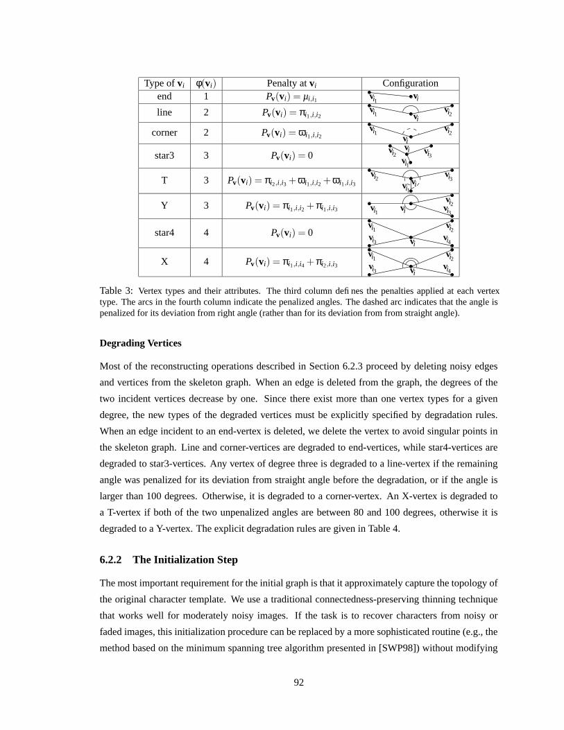
Type of vi φ(vi) Penalty at vi Configurationend 1 Pv(vi) = µi,i1 i1v vi

line 2 Pv(vi) = πi1,i,i2 i1v vi2vi

corner 2 Pv(vi) = ωi1,i,i2i1v vi2

vi

star3 3 Pv(vi) = 0vi vi3

vi2i1v

T 3 Pv(vi) = πi2,i,i3 +ωi1,i,i2 +ωi1,i,i3vi2 vi3vii1v

Y 3 Pv(vi) = πi1,i,i2 +πi1,i,i3 i1vvi2vi vi3

star4 4 Pv(vi) = 0 vi3 vi4

vi2

vi

vi1

X 4 Pv(vi) = πi1,i,i4 +πi2,i,i3 vi3 vi4

vi2

vi

vi1

Table 3: Vertex types and their attributes. The third column defines the penalties applied at each vertextype. The arcs in the fourth column indicate the penalized angles. The dashed arc indicates that the angle ispenalized for its deviation from right angle (rather than for its deviation from from straight angle).

Degrading Vertices

Most of the reconstructing operations described in Section 6.2.3 proceed by deleting noisy edges

and vertices from the skeleton graph. When an edge is deleted from the graph, the degrees of the

two incident vertices decrease by one. Since there exist more than one vertex types for a given

degree, the new types of the degraded vertices must be explicitly specified by degradation rules.

When an edge incident to an end-vertex is deleted, we delete the vertex to avoid singular points in

the skeleton graph. Line and corner-vertices are degraded to end-vertices, while star4-vertices are

degraded to star3-vertices. Any vertex of degree three is degraded to a line-vertex if the remaining

angle was penalized for its deviation from straight angle before the degradation, or if the angle is

larger than 100 degrees. Otherwise, it is degraded to a corner-vertex. An X-vertex is degraded to

a T-vertex if both of the two unpenalized angles are between 80 and 100 degrees, otherwise it is

degraded to a Y-vertex. The explicit degradation rules are given in Table 4.

6.2.2 The Initialization Step

The most important requirement for the initial graph is that it approximately capture the topology of

the original character template. We use a traditional connectedness-preserving thinning technique

that works well for moderately noisy images. If the task is to recover characters from noisy or

faded images, this initialization procedure can be replaced by a more sophisticated routine (e.g., the

method based on the minimum spanning tree algorithm presented in [SWP98]) without modifying

92

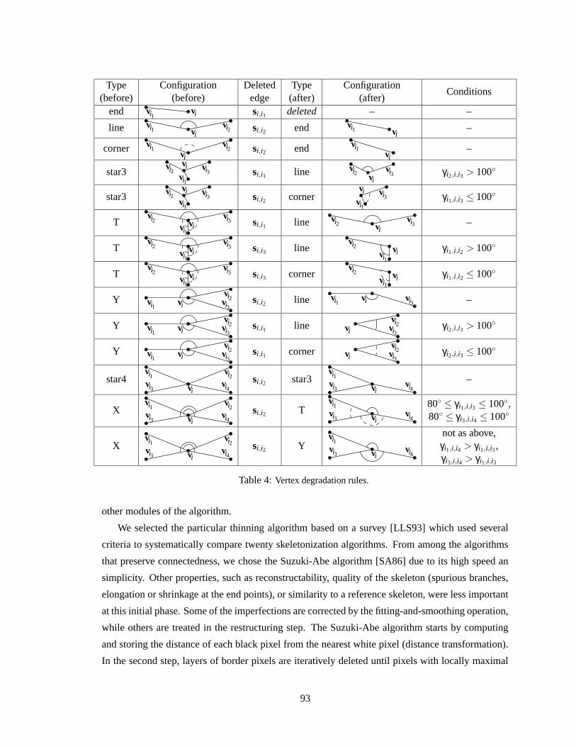
Type(before)

Configuration(before)

Deletededge

Type(after)

Configuration(after)

Conditions

end i1v vi si,i1 deleted – –

line i1v vi2visi,i2 end i1v

vi–

corner i1v vi2vi

si,i2 end i1vvi

–

star3vi vi3

vi2i1v si,i1 line vi3

vi2 viγi2,i,i3 > 100◦

star3vi vi3

vi2i1v si,i2 corner

vi vi3i1v γi1,i,i3 ≤ 100◦

Tvi2 vi3vii1v si,i1 line vi

vi2 vi3 –

Tvi2 vi3vii1v si,i3 line vi

vi2

i1vγi1,i,i2 > 100◦

Tvi2 vi3vii1v si,i3 corner vi

vi2

i1vγi1,i,i2 ≤ 100◦

Y i1vvi2vi vi3

si,i2 line i1v vi vi3 –

Y i1vvi2vi vi3

si,i1 linevi2vi vi3

γi2,i,i3 > 100◦

Y i1vvi2vi vi3

si,i1 cornervi2vi vi3

γi2,i,i3 ≤ 100◦

star4 vi3 vi4

vi2

vi

vi1 si,i2 star3 vi3 vi4vi

vi1 –

X vi3 vi4

vi2

vi

vi1 si,i2 T vi3 vi4vi

vi1 80◦ ≤ γi1,i,i3 ≤ 100◦,80◦ ≤ γi3,i,i4 ≤ 100◦

X vi3 vi4

vi2

vi

vi1 si,i2 Y vi3 vi4vi

vi1not as above,γi1,i,i4 > γi1,i,i3 ,γi3,i,i4 > γi1,i,i3

Table 4: Vertex degradation rules.

other modules of the algorithm.

We selected the particular thinning algorithm based on a survey [LLS93] which used several

criteria to systematically compare twenty skeletonization algorithms. From among the algorithms

that preserve connectedness, we chose the Suzuki-Abe algorithm [SA86] due to its high speed an

simplicity. Other properties, such as reconstructability, quality of the skeleton (spurious branches,

elongation or shrinkage at the end points), or similarity to a reference skeleton, were less important

at this initial phase. Some of the imperfections are corrected by the fitting-and-smoothing operation,

while others are treated in the restructuring step. The Suzuki-Abe algorithm starts by computing

and storing the distance of each black pixel from the nearest white pixel (distance transformation).

In the second step, layers of border pixels are iteratively deleted until pixels with locally maximal

93

distance values are reached. Finally, some of the remaining pixels are deleted so that connectedness

is preserved and the skeleton is of width one.

After thinning the template, an initial skeleton graph is computed (Figure 31). In general, mid-

points of pixels of the skeleton are used as vertices of the graph, and two vertices are connected by

an edge if the corresponding pixels are eight-neighbors, i.e., if they have at least one common corner.

To avoid short circles and crossing edges near junctions of the skeleton, neighboring junction pixels

(pixels having more than two eight-neighbors) are recursively placed into pixel-sets. For such a set,

only one vertex is created in the center of gravity of the pixels’ midpoints. This junction-vertex is

then connected to vertices representing pixels neighboring to any of the junction pixels in the set. In

this initial phase, only end, line, star3, and star4-vertices are used depending on whether the degree

of the vertex is one, two, three, or four, respectively. In the rare case when a vertex representing a

set of junction pixels has more than four neighbors, the neighbors are split into two or more sets of

two or three vertices. Each neighbor in a set is then connected to a mutual junction-vertex, and the

created junction-vertices are connected to each other. The circled vertices in Figures 31(c) and (d)

demonstrate this case.

6.2.3 The Restructuring Step

The restructuring step complements the two fitting-and-smoothing steps. In the fitting-and-smoothing

step we relocate vertices and edges of the skeleton graph based on their positions relative to the tem-

plate, but we do not modify the skeleton graph in a graph theoretical sense. In the restructuring step

we use geometric properties of the skeleton graph to modify the configuration of vertices and edges.

We do not explicitly use the template, and we do not move vertices and edges of the skeleton graph

in this step.

The double purpose of the restructuring step is to eliminate or rectify imperfections of the initial

skeleton graph, and to simplify the skeletal description of the template. Below we define operations

that can be used to modify the configuration of the skeleton graph. Since the types of the imperfec-

tions depend on properties of both the input data and the initialization method, one should carefully

select the particular operations and set their parameters according to the specific application. At

the description of the operations, we give approximate values for each parameter based on our ex-

periments with a wide variety of real data. Specific settings will be given in Section 6.3 where we

present the results of two particular experiments.

For the formal description of the restructuring operations, we define some simple concepts.

We call a list of vertices pi1,...,i` = (vi1 , . . . ,vi`), ` > 1 a path if each pair of consecutive vertices

(vi j ,vi j+1), j = 1, . . . , `− 1 is connected by an edge. A loop is a path pi1,...,i` such that i1 = i` and

none of the inner vertices vi2 , . . . ,vi`−1 are equal to each other or to vi1 . The length of a path is

94

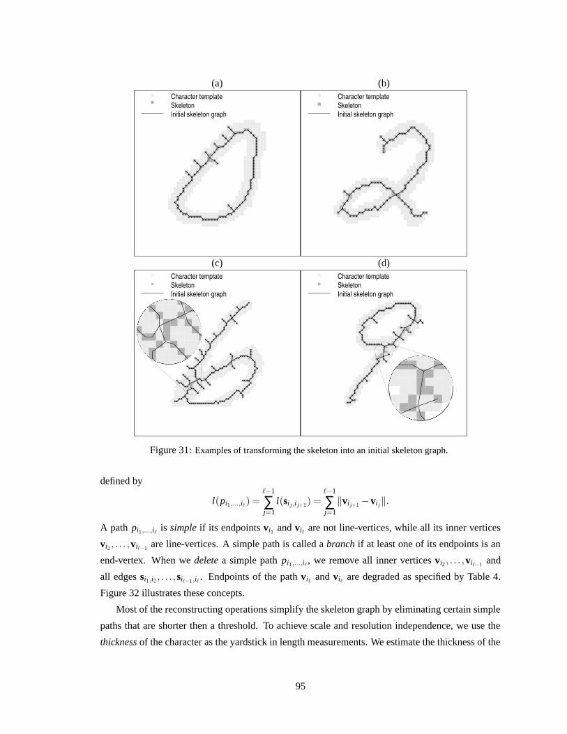
(a)Character templateSkeletonInitial skeleton graph

(b)Character templateSkeletonInitial skeleton graph

(c)Character templateSkeletonInitial skeleton graph

(d)Character templateSkeletonInitial skeleton graph

Figure 31: Examples of transforming the skeleton into an initial skeleton graph.

defined by

l(pi1,...,i`) =`−1

∑j=1

l(si j,i j+1) =`−1

∑j=1

‖vi j+1 −vi j‖.

A path pi1,...,i` is simple if its endpoints vi1 and vi` are not line-vertices, while all its inner vertices

vi2 , . . . ,vi`−1 are line-vertices. A simple path is called a branch if at least one of its endpoints is an

end-vertex. When we delete a simple path pi1,...,i` , we remove all inner vertices vi2 , . . . ,vi`−1 and

all edges si1,i2 , . . . ,si`−1,i` . Endpoints of the path vi1 and vi` are degraded as specified by Table 4.

Figure 32 illustrates these concepts.

Most of the reconstructing operations simplify the skeleton graph by eliminating certain simple

paths that are shorter then a threshold. To achieve scale and resolution independence, we use the

thickness of the character as the yardstick in length measurements. We estimate the thickness of the

95

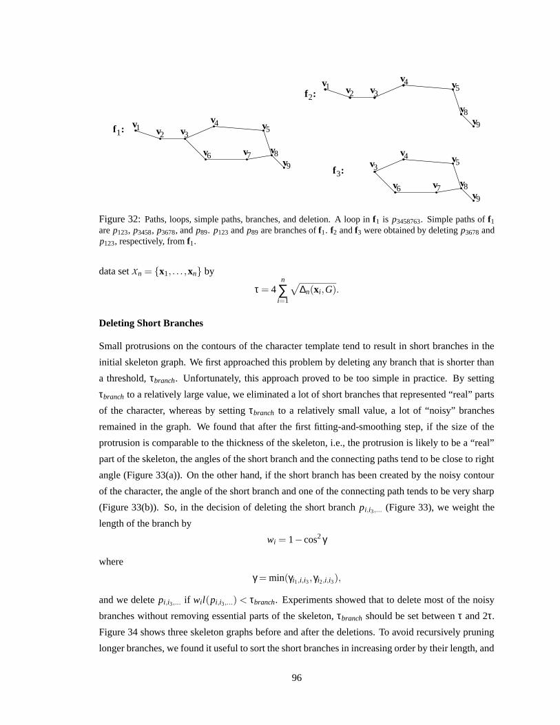
v4 v5

v6 v7 v8v9

v3

v4 v5v1

v8v9

v2

v3

v4 v5

v6 v7

v1

v8v9

v2

v33f :

2

1f :

f :

Figure 32: Paths, loops, simple paths, branches, and deletion. A loop in f1 is p3458763. Simple paths of f1

are p123, p3458, p3678, and p89. p123 and p89 are branches of f1. f2 and f3 were obtained by deleting p3678 andp123, respectively, from f1.

data set Xn = {x1, . . . ,xn} by

τ = 4n

∑i=1

√

∆n(xi,G).

Deleting Short Branches

Small protrusions on the contours of the character template tend to result in short branches in the

initial skeleton graph. We first approached this problem by deleting any branch that is shorter than

a threshold, τbranch. Unfortunately, this approach proved to be too simple in practice. By setting

τbranch to a relatively large value, we eliminated a lot of short branches that represented “real” parts

of the character, whereas by setting τbranch to a relatively small value, a lot of “noisy” branches

remained in the graph. We found that after the first fitting-and-smoothing step, if the size of the

protrusion is comparable to the thickness of the skeleton, i.e., the protrusion is likely to be a “real”

part of the skeleton, the angles of the short branch and the connecting paths tend to be close to right

angle (Figure 33(a)). On the other hand, if the short branch has been created by the noisy contour

of the character, the angle of the short branch and one of the connecting path tends to be very sharp

(Figure 33(b)). So, in the decision of deleting the short branch pi,i3,... (Figure 33), we weight the

length of the branch by

wi = 1− cos2 γ

where

γ = min(γi1,i,i3 ,γi2,i,i3),

and we delete pi,i3,... if wil(pi,i3,...) < τbranch. Experiments showed that to delete most of the noisy

branches without removing essential parts of the skeleton, τbranch should be set between τ and 2τ.

Figure 34 shows three skeleton graphs before and after the deletions. To avoid recursively pruning

longer branches, we found it useful to sort the short branches in increasing order by their length, and

96

deleting them in that order. This was especially important in the case of extremely noisy skeleton

graphs such as depicted by Figures 34(a) and (b).

vivi1vi2vivi1

vi2

vi3 vi3

(a) (b)

Figure 33: If the protrusion is a “real” part of the skeleton, the angles of the short branch and the connectingpaths tend to be close to right angle (a), whereas if the short branch has been created by a few noisy pixelson the contour of the character, the short branch tends to slant to one of the connecting paths during the firstfitting-and-smoothing step (b).

Removing Short Loops

Short loops created by thinning algorithms usually indicate isolated islands of white pixels in the

template. We remove any loop from the skeleton graph if its length is below a threshold τloop. A

loop is removed by deleting the longest simple path it contains. Experiments showed that to remove

most of the noisy loops without removing essential parts of the skeleton, τloop should be set between

2τ and 3τ. Figure 35 shows three skeleton graphs before and after the operation.

Merging Star3-Vertices

In experiments we found that if two penstrokes cross each other at a sharp angle, the thinning

procedure tends to create two star3-vertices connected by a short simple path rather then a star4-

vertex. The first approach to correct this imperfection was to merge any two star3-vertices that are

connected by a simple path shorter than a threshold, τstar3. Unfortunately, this approach proved to

be too simple in practice. By setting τstar3 to a relatively large value, we eliminated a lot of short

paths that were not created by crossing penstrokes, whereas by setting τstar3 to a relatively small

value, a lot of paths created by crossing penstrokes remained in the graph. We found that it is more

likely that the short path pi,..., j (Figure 36) is created by two crossing penstrokes if the angles γi1,i,i2

and γ j1, j, j2 are small. To avoid merging vi and v j when these two angles are large, we weight the

length of the path pi,..., j by an experimentally developed factor

wi j =

[

(1− cosγi1,i,i2)+(1− cosγ j1, j, j2)

4

]3

,

and we merge vi and v j if wi jl(pi,..., j) < τstar3. When merging two star3-vertices vi and v j, we first

delete the path pi,..., j, and remove vi and v j. Then we add a new vertex vnew and connect the four

97




Character templateSkeleton graph



Figure 34: Deleting short branches. Skeleton graphs before (top row) and after (bottom row) the deletion.

remaining neighbors of vi and v j to vnew (Figure 36). Experiments indicated that for the best results

τstar3 should be set between 0.5τ and τ. Figure 37 shows three skeleton graphs before and after the

merge.

Updating Star3 and Star4-Vertices

Initially, all the junction-vertices of the skeleton are either star3 or star4-vertices. After the skele-

ton has been smoothed by the first fitting-and-smoothing step and cleaned by the restructuring op-

erations described above, we update the junction-vertices of the skeleton to Y, T and X-vertices

depending on the local geometry of the junction-vertices and their neighbors. A star4-vertex is al-

ways updated to an X-vertex. When updating a star3-vertex, we face the same situation as when

degrading an X-vertex, so a star3-vertex is updated to a T-vertex if two of the angles at the vertex

are between 80 and 100 degrees, otherwise it is updated to a Y-vertex. The formal rules are given in

the last two rows of Table 4.

98







Figure 35: Removing short loops. Skeleton graphs before (top row) and after (bottom row) the removal.

Filtering Vertices

In this step, we iteratively remove every line-vertex whose two incident edges are shorter than a

threshold τ f ilter. Formally, any line-vertex v j is removed from the graph if

‖v j −vi‖ < τ f ilter and ‖v j −v`‖ < τ f ilter

where vi and v` are the neighbors of v j. When a line-vertex v j is removed, the two edges incident

to v j, si j and s j`, are also removed. Then the two former neighbors of v j are connected by a new

edge (Figure 38).

Filtering vertices is an optional operation. It can be used to speed up the optimization if the

character template has a high resolution since in this case the initial skeleton graph has much more

vertices than it is needed for reasonably smooth approximation. It can be also used after the opti-

mization to improve the compression rate if the objective is to compress the image by storing the

character skeleton instead of the template. In this case the filtering operation can be coupled with a

smoothing operation at the other end where the character is recovered based on the skeleton graph

(see Section 6.3.2). Figure 39 shows an example of a skeleton graph before and after the filtering

operation.

99

vi

vi1

vi2vj

vj2

v1j vi1

vi2 vj2

v1

vnew

Before:

j

After:

Figure 36: When merging two star3-vertices, we remove the vertices and the path connecting them. Thenwe add a new vertex and connect the former neighbors of the two star3-vertices to the new vertex.

6.3 Experimental Results

6.3.1 Skeletonizing Isolated Digits

In this section we report results on isolated hand-written digits from the NIST Special Database

19 [Gro95]. To set the parameters and to tune the algorithm, we chose 100 characters per digit

randomly. Figures 40 through 49 display eight templates for each digit. These examples were

chosen so that they roughly represent the 100 characters both in terms of the variety of the input data

and in terms of the success rate of the algorithm. To illuminate the contrast between the pixelwise

skeleton of the character and the skeleton graph produced by the principal graph algorithm, we show

the initial graph (upper row in each figure) and the final graph (lower row in each figure) for each

chosen character template. The length thresholds of the restructuring operations were set to the

values indicated by Table 5.

τbranch τloop τstar3 τ f ilter

1.2τ 3τ τ τ

Table 5: Length thresholds of the restructuring operations in experiments with isolated digits.

The results indicate that the principal graph algorithm finds a smooth medial axis of the great

majority of the characters. In the few cases when the skeleton graph is imperfect, we could identify

two sources of errors. The first cause is that, obviously, the restructuring operations do not work

perfectly for all the characters. For instance, short branches can be cut (Figure 46(a)), short loops

can be eliminated (Figure 42(c)), or star3-vertices can be merged mistakenly (Figure 44(h)). To

correct these errors, one has to include some a-priori information in the process, such as a collection

of possible configurations of skeleton graphs that can occur in hand-written digits. The other source

of errors is that at this phase, we do not have restructuring operations that add components to the

skeleton graph. For instance, skeleton graphs in Figures 42(e) and 48(d) could be improved by

connecting broken lines based on the closeness of their endpoints. One could also add short paths

to create branches or loops that were missing from the initial graph (Figures 42(b) and 48(f)). This

operation could be based on local thickness measurements along the graph that could point out

protrusions caused by overlapping lines in the character. The exact definitions and implementations

100







Figure 37: Merging star3-vertices. Skeleton graphs before (top row) and after (bottom row) the merge.

vvj

vli v vli

After:Before:

Figure 38: Removing the line-vertex v j in the filtering operation.

of these operations are subjects of future research.

101




Figure 39: Filtering vertices. A skeleton graph (a) before filtering, (b) after filtering with τf ilter = 1, and (b)after filtering with τf ilter = 2.

(a)0:0

(b)0:2

(c)0:10

(d)0:18

(e)0:31

(f)0:55

(g)0:60

(h)0:67

Figure 40: Skeleton graphs of isolated 0’s. Initial (upper row) and final (lower row) skeletons.

(a)1:19

(b)1:30

(c)1:35

(d)1:36

(e)1:57

(f)1:62

(g)1:81

(h)1:91


102

(a)2:0

(b)2:13

(c)2:22

(d)2:35

(e)2:48

(f)2:56

(g)2:75

(h)2:83


(a)3:14

(b)3:21

(c)3:29

(d)3:33

(e)3:49

(f)3:61

(g)3:66

(h)3:92


(a)4:11

(b)4:25

(c)4:28

(d)4:35

(e)4:37

(f)4:56

(g)4:63

(h)4:71


(a)5:1

(b)5:13

(c)5:35

(d)5:53

(e)5:55

(f)5:59

(g)5:86

(h)5:92


103

(a)6:1

(b)6:2

(c)6:24

(d)6:35

(e)6:52

(f)6:54

(g)6:61

(h)6:94


(a)7:9

(b)7:18

(c)7:32

(d)7:45

(e)7:47

(f)7:52

(g)7:67

(h)7:81


(a)8:3

(b)8:7

(c)8:13

(d)8:28

(e)8:56

(f)8:59

(g)8:62

(h)8:74


(a)9:0

(b)9:19

(c)9:25

(d)9:36

(e)9:39

(f)9:51

(g)9:56

(h)9:80


104

6.3.2 Skeletonizing and Compressing Continuous Handwriting

In this section we present results of experiments with images of continuous handwriting. We used

the principal graph algorithm to skeletonize short pangrams (sentences that contain all the letters of

the alphabet) written by different individuals. The emphasis in these experiments was on using the

skeleton graph for representing hand-written text efficiently.

Figure 50 shows the images of two pangrams written by two individuals. For the sake of easy

referencing, hereafter we will call them Alice (Figure 50(a)) and Bob (Figure 50(b)). After scanning

the images, the principal graph algorithm was used to produce the skeleton graphs depicted by

Figure 51. Since the images were much cleaner than the images of isolated digits used in the

previous section, τbranch and τloop were set slightly lower than in the previous experiments. We

also found that the incorrect merge of two star3-vertices has a much worse visual effect than not

merging two star3-vertices when they should be merged, so we set τstar3 to half of the value that

was used in the experiments with isolated digits. Finally, we did not use filtering vertices in the

restructuring step. The length thresholds of the restructuring operations were set to the values

indicated by Table 6. The thickness of each curve in Figure 51 was set to the estimated thickness τof the template.

τbranch τloop τstar3 τ f ilter

τ 2τ 0.5τ 0

Table 6: Length thresholds of the restructuring operations in experiments with continuous handwriting.τ f ilter = 0 indicates that we did not filter vertices in the reconstruction step.

(a) (b)

Figure 50: Original images of continuous handwritings. (a) Alice, (b) Bob.

To demonstrate the efficiency of representing the texts by their skeleton graphs, we applied the

vertex filtering operation after the skeleton graphs were produced. For achieving high compression

rate, τ f ilter should be set to a relatively large value to remove most of the line-vertices from the

skeleton graph. Since filtering with a large threshold has an unfortunate visual effect of producing

sharp-angled polygonal curves (see Figure 39(c)), we fit cubic splines through the vertices of each

path of the skeleton graph. Tables 7 and 8 show the results.

105

(a)


(b)


Figure 51: Skeleton graphs of continuous handwritings. (a) Alice, (b) Bob.

To be able to compute the number of bytes needed for storing the images, in the compression

routine we also set the number of bits nb used to store each coordinate of a vertex. The vertices are

stored consecutively with one bit sequence of length nb marking the end of a path. So, for example,

when nb is set to 8, the vertices of the skeleton graph are rounded to the points of a 255× 255

rectangular grid, and the remaining byte is used to mark the end of a path. By using this scheme,

the skeleton graph can be stored by using

N =⌈

(np +2m)nb/8⌉

bytes where np is the number of paths and m is the number of vertices. Tables 7 and 8 show the

skeleton graphs and the number of bytes needed to store the images. The numbers of paths in

Alice’s and Bob’s texts are 148 and 74, respectively. As a comparison, the size of the raw bitmap

compressed by using the Lempel-Ziv algorithm (gzip under UNIX) is 2322 bytes in Alice’s case,

and 1184 bytes in Bob’s case. So, for instance, if the filter threshold is set to 6τ, and 8 bits are

used to store the coordinates of the vertices, the algorithm produces a skeleton that approximates

the original text quite well while compressing the image to less than half of the size of the gzipped

raw bitmap. Note that the bit sequence representing the skeleton graph can be further compressed

by using traditional compression methods.

106

τ f ilter m nb = 8 nb = 6Skeleton graph N Skeleton graph N

2τ 743 1634 – –

4τ 492 1132 – –

6τ 408 964 723

10τ 361 870 653

20τ 324 796 597

Table 7: Compression of Alice’s handwriting. m is the number of vertices, nb is the number of bits used tostore each coordinate of a vertex, and N is the total number of bytes needed to store the skeleton graph of theimage.

107

τ f ilter m nb = 8 nb = 6Skeleton graph N Skeleton graph N

2τ 435 944 – –

4τ 280 634 – –

6τ 225 524 393

10τ 195 464 348

20τ 173 420 315

Table 8: Compression of Bob’s handwriting. m is the number of vertices, nb is the number of bits used tostore each coordinate of a vertex, and N is the total number of bytes needed to store the skeleton graph of theimage.

108

Chapter 7

Conclusion

The three pillars of the thesis are the theoretical results described in Chapter 4, the polygonal line

algorithm proposed in Chapter 5, and the experimental results with the principal graph algorithm

presented in Chapter 6. Below we summarize our main results in these three areas, and briefly

discuss some of the possible areas of future research.

Theory

We proposed a new definition of principal curves with a length constraint. Based on the new defini-

tion, we proved the following two results.

• Existence of principal curves. Principal curves in the new sense exist for all distributions

with final second moments.

• Consistency and rate of convergence. For distributions concentrated on a bounded and

closed convex set, an estimator of the principal curve can be constructed based on a data set

of n i.i.d. sample points such that the expected loss of the estimator converges to the loss of

the principal curve at a rate of n−1/3.

Two interesting open problems are the following.

• Concrete principal curves. It would be of both theoretical and practical interest if concrete

examples of principal curves of basic multivariate densities could be found.

• A more practical constraint. It would be convenient to replace the length constraint with a

practically more suitable restriction, such as a limit on the maximum curvature of the curve,

that is more closely related to the curvature penalty applied in the practical algorithm.

109

Algorithm

Our main result here is a practical algorithm to estimate principal curves based on data. Experimen-

tal results on simulated data demonstrate that the polygonal line algorithm compares favorably to

previous methods both in terms of performance and computational complexity.

A possible area of further research is to extend the polygonal line algorithm to find multi-

dimensional manifolds. There are two fundamentally different approaches to extend principal

curves to principal surfaces or to arbitrary-dimensional principal manifolds. In the first approach,

the theoretical model and the algorithm are either extended to include smooth non-parametric sur-

faces [Has84, HS89], or they can be used, without modification, to find arbitrary-dimensional prin-

cipal manifolds [SMS98, SWS98]. The second approach follows the strategy of an iterative PCA

algorithm which finds the ith largest principal component by finding the first principal component

in the linear subspace orthogonal to the first i− 1 principal components. In the second approach,

therefore, the one-dimensional principal curve routine is called iteratively so that in ith iteration,

we compute the principal curve of the data set obtained by subtracting from the data points their

projections to the principal curve computed in the (i−1)th iteration [Del98, CG98b, DM95].

Theoretically, it is not impossible to use the first approach, i.e., to extend the polygonal line

algorithm to find arbitrary-dimensional piecewise linear manifolds. Technically, however, it is not

clear at this point how this extension could be done. The second approach, on the other hand, seems

feasible to be implemented with the polygonal line algorithm. The exact design of the algorithm is

subject of future research.

Applications

We proposed an extended version of the polygonal line algorithm to find principal graphs of data sets

obtained from binary templates of black-and-white images. Test results indicate that the principal

graph algorithm can be used to find a smooth medial axis of a wide variety of character templates,

and to represent hand-written text efficiently.

Here, the main objective of future research is to improve the computational complexity of the

method. At this point the “general purpose” polygonal line algorithm is used as the “main engine”

for the principal graph algorithm. We expect that by incorporating the special features of the highly

structured data obtained from binary templates into the algorithm, the efficiency of the algorithm

can be increased substantially.

110

Bibliography

[AH69] T. M. Alcorn and C. W. Hoggar. Preprocessing of data for character recognition. Mar-

coni Review, 32:61–81, 1969.

[Ale84] K. Alexander. Probability inequalities for empirical processes and a law of the iterated

logarithm. Annals of Probability, pages 1041–1067, 1984.

[Ash72] R. B. Ash. Real Analysis and Probability. Academic Press, New York, 1972.

[Bar87] D. J. Bartholomew. Latent Variable Models and Factor Analysis. Charles Griffin &

Co. Ltd., London, 1987.

[BCJL94] P. V. Balakrishnan, M. C. Cooper, V. S. Jacob, and P. A. Lewis. A study of the classifi-

cation capabilities of neural networks using unsupervised learning: a comparison with

k-means clustering. Psychometrika, 59(4):509–525, 1994.

[BD75] J. Bezdek and J. Dunn. Optimal fuzzy partitions: A heuristic for estimating the parame-

ters in a mixture of normal distributions. IEEE Transactions on Computers, 24(4):835–

838, 1975.

[BDHW97] G. Balzuweit, R. Der, M. Herrmann, and M. Welk. An algorithm for generalized

principal curves with adaptive topology in complex data sets. Technical Report 3/97,

Institut fur Informatik, Universitat Leipzig, 1997.

[BLL98] P. Bartlett, T. Linder, and G. Lugosi. The minimax distortion redundancy in empirical

quantizer design. IEEE Transactions on Information Theory, 44(5):1802–1813, 1998.

[BP95] J. C. Bezdek and N. R. Pal. An index of topological preservation for feature extraction.

Pattern Recognition, 28(3):381–391, 1995.

[BR92] J. D. Banfield and A. E. Raftery. Ice floe identification in satellite images using math-

ematical morphology and clustering about principal curves. Journal of the American

Statistical Association, 87:7–16, 1992.

111

[BSW96] C. M. Bishop, M. Svensen, and C. K. I. Williams. EM optimization of latent-variables

density models. In David S. Touretzky, Michael C. Mozer, and Michael E. Hasselmo,

editors, Advances in Neural Information Processing Systems, volume 8, pages 465–

471. The MIT Press, 1996.

[BSW98] C. M. Bishop, M. Svensen, and C. K. I. Williams. GTM: The generative topographic

mapping. Neural Computation, 10(1):215–235, 1998.

[BT98] C. M. Bishop and M. E. Tipping. A hierarchical latent variable model for data visual-

ization. IEEE Transactions on Pattern Analysis and Machine Intelligence, 20(3):281–

293, 1998.

[CG92] G. Celeux and G. Govaert. A classification EM algorithm and two stochastic versions.

Computational Statistics and Data Analysis, 14:315–332, 1992.

[CG98a] K. Chang and J. Ghosh. Principal curve classifier – a nonlinear approach to pattern

classification. In IEEE International Joint Conference on Neural Networks, pages

695–700, Anchorage, AL, May 5–9 1998.

[CG98b] K. Chang and J. Ghosh. Principal curves for nonlinear feature extraction and classifi-

cation. In Applications of Artificial Neural Networks in Image Processing III, volume

3307, pages 120–129, San Jose, CA, Jan 24–30 1998. SPIE Photonics West ’98 Elec-

tronic Image Conference.

[Cho94] P. A. Chou. The distortion of vector quantizers trained on n vectors decreases to the

optimum as op(1/n). In Proceedings of IEEE International Symposium on Information

Theory, Trondheim, Norway, 1994.

[Cle79] W. S. Cleveland. Robust locally weighted regression and smoothing scatterplots. Jour-

nal of the American Statistical Association, 74:829–835, 1979.

[DBH96] R. Der, G. Balzuweit, and M. Herrmann. Constructing principal manifolds in sparse

data sets by self-organizing maps with self-regulating neighborhood width. In Pro-

ceedings of the International Conference on Neural Networks, pages 480–483, 1996.

[Del98] P. Delicado. Principal curves and principal oriented points. Technical Report 309,

Department d’Economia i Empresa, Universitat Pompeu Fabra, 1998.

[Deu68] E. S. Deutsch. Preprocessing for character recognition. In Proceedings of the IEE NPL

Conference on Pattern Recognition, pages 179–190, 1968.

112

[DGL96] L. Devroye, L. Gyorfi, and G. Lugosi. A Probabilistic Theory of Pattern Recognition.

Springer, New York, 1996.

[Din55] G. P. Dinnen. Programming pattern recognition. In Proceedings of the Western Joint

Computer Conference, pages 94–100, New York, 1955.

[DK82] P. A. Devijver and J. Kittler. Pattern Recognition: a Statistical Approach. Prentice

Hall, Englewood Cliffs, New Jersey, 1982.

[DLR77] A.P. Dempster, N. M. Laird, and D. B. Rubin. Maximum likelihood from incomplete

data via the EM algorithm. Journal of the Royal Statistical Society Series B, 39:1–38,

1977.

[DM95] D. Dong and T. J. McAvoy. Nonlinear principal component analysis – based on prin-

cipal curves and neural networks. Computers Chem. Engineering, 20(1):65–78, 1995.

[DP97] A. Datta and S. K. Parui. Skeletons from dot patterns: A neural network approach.

Pattern Recognition Letters, 18:335–342, 1997.

[DS96a] T. Duchamp and W. Stuetzle. Extremal properties of principal curves in the plane.

Annals of Statistics, 24(4):1511–1520, 1996.

[DS96b] T. Duchamp and W. Stuetzle. Geometric properties of principal curves in the plane. In

Helmut Rieder, editor, Robust statistics, data analysis, and computer intensive meth-

ods: in honor of Peter Huber’s 60th birthday, volume 109 of Lecture notes in statistics,

pages 135–152. Springer-Verlag, 1996.

[EOS92] E. Erwin, K. Obermayer, and K. Schulten. Self-organizing maps: ordering, conver-

gence properties and energy functions. Biological Cybernetics, 67:47–55, 1992.

[Eve84] B. S. Everitt. An Introduction to Latent Variable Models. Chapman and Hall, London,

1984.

[Fle97] A. Flexer. Limitations of self-organizing maps for vector quantization and multidi-

mensional scaling. In M. C. Mozer, M. I. Jordan, and T. Petsche, editors, Advances

in Neural Information Processing Systems: Proceedings of the 1996 Conference, vol-

ume 9, pages 445–451. MIT Press, 1997.

[Fle99] A Flexer. On the use of self-organizing maps for clustering and visualization. In J.M.

Zytkow and J. Rauch, editors, Principles of Data Mining and Knowledge Discovery,

Third European Conference, PKDD’99, Lecture Notes in Artificial Intelligence 1704,

pages 80–88, Prague, Czech Republic, 1999. Springer.

113

[Fol89] P. Foldiak. Adaptive network for optimal linear feature extraction. In IEEE Press,

editor, Proceedings of the IEEE/INNS International Joint Conference on Neural Net-

works, volume 1, pages 401–405, New York, 1989.

[GG92] A. Gersho and R. M. Gray. Vector Quantization and Signal Compression. Kluwer,

Boston, 1992.

[GKL80] R. M. Gray, J. C. Kieffer, and Y. Linde. Locally optimal block quantizer design. Infor-

mation and Control, 45:178–198, May 1980.

[Gro95] P. Grother. NIST Special Database 19. National Institute of Standards and Technology,

Advanced Systems Division, 1995.

[Har75] J. A. Hartigan. Clustering Algorithms. Wiley, New York, 1975.

[Has84] T. Hastie. Principal curves and surfaces. PhD thesis, Stanford University, 1984.

[Hoe63] W. Hoeffding. Probability inequalities for sums of bounded random variables. Journal

of the American Statistical Association, 58:13–30, 1963.

[Hot33] H. Hotelling. Analysis of a complex of statistical variables into principal components.

Journal of Educational Psychology, 24:417–441, 498–520, 1933.

[HS89] T. Hastie and W. Stuetzle. Principal curves. Journal of the American Statistical Asso-

ciation, 84:502–516, 1989.

[JD88] A. K. Jain and R. C. Dubes. Algorithms for Clustering Data. Prentice Hall, Englewood

Cliffs, New Jersey, 1988.

[JW92] R. A. Johnson and D. W. Wichern. Applied Multivariate Statistical Analysis. Prentice

Hall, Englewood Cliffs, New Jersey, 1992.

[Kar47] K. Karhunen. Uber lineare methoden in der wahrscheinlichkeitsrechnung. Amer. Acad.

Sci., Fennicade, Ser. A, I, 37:3–79, 1947. (Translation: RAND Corporation, Santa

Monica, California, Rep. T-131, Aug. 1960).

[KCRU57] R. A. Kirsh, L. Cahn, C. Ray, and G. J. Urban. Experiment in processing pictorial

information with a digital computer. In Proceedings of the Eastern Joint Computer

Conference, pages 221–229, New York, 1957.

[KKLZ] B. Kegl, A. Krzyzak, T. Linder, and K. Zeger. Principal curves: Learning and conver-

gence. In Proceedings of IEEE International Symposium on Information Theory, page

387, Cambridge, Mass., Aug. 1998.

114

[KKLZ99] B. Kegl, A. Krzyzak, T. Linder, and K. Zeger. A polygonal line algorithm for con-

structing principal curves. In Advances in Neural Information Processing Systems,

volume 11, pages 501–507, Denver, Col., Nov. 1998, 1999. The MIT Press.

[KKLZ00] B. Kegl, A. Krzyzak, T. Linder, and K. Zeger. Learning and design of principal

curves. IEEE Transactions on Pattern Analysis and Machine Intelligence, 22(3):281–

297, 2000.

[Koh82] T. Kohonen. Clustering, taxonomy, and topological maps of patterns. In Proceedings

of the 6th International Conference on Pattern Recognition, pages 114–128, Munich,

1982.

[Koh97] T. Kohonen. The Self-Organizing Map. Springer-Verlag, 2nd edition, 1997.

[KR95] R. E. Kass and A. E. Raftery. Bayes factors. Journal of the American Statistical

Association, pages 773–795, 1995.

[Kra91] M.A. Kramer. Nonlinear principal component analysis using autoassociative neural

networks. AIChE Journal, 37(2):233–243, 1991.

[KT61] A. N. Kolmogorov and V. M. Tikhomirov. ε-entropy and ε-capacity of sets in function

spaces. Translations of the American Mathematical Society, 17:277–364, 1961.

[KW78] J. B. Kruskal and M. Wish. Multidimensional scaling. In Sage University Paper Series

on Quantitative Applications in the Social Sciences, number 07-011. Sage Publica-

tions, Beverly Hills, California, 1978.

[LBG80] Y. Linde, A. Buzo, and R. M. Gray. An algorithm for vector quantizer design. IEEE

Transactions on Communications, COM-28(1):84–95, 1980.

[LLS93] S. W. Lee, L. Lam, and C.Y. Suen. A systematic evaluation of skeletonization al-

gorithms. International Journal of Pattern Recognition and Artificial Intelligence,

7(5):1203–1225, 1993.

[LLZ94] T. Linder, G. Lugosi, and K. Zeger. Rates of convergence in the source coding theorem,

in empirical quantizer design and in universal lossy source coding. IEEE Transactions

on Information Theory, 40:1728–1740, 1994.

[Lut90] S. P. Luttrell. Derivation of a class of training algorithms. IEEE Transactions on

Neural Networks, 1(2):229–232, 1990.

115

[Mac67] J. MacQueen. Some methods for classification and analysis of multivariate observa-

tions. In Proceedings of the Fifth Berkeley Symposium on Mathematics, Statistics and

Probability, pages 281–296, 1967.

[Mac95] D. J. C. MacKay. Bayesian neural networks and density networks. Nuclear Instruments

and Methods in Physics Research, 354(1):73–80, 1995.

[MAG91] S. Mahmoud, I. Abuhaiba, and R. Green. Skeletonization of arabic characters using

clustering based skeletonization algorithm (CBSA). Pattern Recognition, 24(5):453–

464, 1991.

[MC95] F. Mulier and V. Cherkassky. Self-organization as an iterative kernel smoothing pro-

cess. Neural Computation, 7:1165–1177, 1995.

[MMT95] E. C. Malthouse, R. H. S. Mah, and A. C. Tamhane. Some theoretical results on nonlin-

ear principal component analysis. In Proceedings of the American Control Conference,

pages 744–748, June 1995.

[MZ97] N. Merhav and J. Ziv. On the amount of side information required for lossy data

compression. IEEE Transactions on Information Theory, 43:1112–1121, 1997.

[NS84] N. J. Naccache and R. Shingal. SPTA: A proposed algorithm for thinning binary pat-

terns. IEEE Transactions on Systems, Man and Cybernetics, 14(3), 1984.

[Oja92] E. Oja. Principal components, minor components, and linear neural networks. Neural

Networks, 5:927–935, 1992.

[O’N66] B. O’Neil. Elementary Differential Geometry. Academic Press, Inc., Orlando, Florida,

1966.

[Pav80] T. Pavlidis. A thinning algorithm for discrete binary images. Computer Graphics and

Image Processing, 13(2):142–157, 1980.

[Pea01] K. Pearson. On lines and planes of closest fit to systems of points in space. Philos.

Mag., 6(2):559–572, 1901.

[Pol81] D. Pollard. Strong consistency of k-means clustering. Annals of Statistics, 9:135–140,

1981.

[Pol82] D. Pollard. A central limit theorem for k-means clustering. Annals of Probability,

10:919–926, 1982.

116

[RMS92] H. Ritter, T. Martinetz, and K. Schulten. Neural Computation and Self-Organizing

Maps: An Introduction. Addison-Wesley, Reading, Massachusetts, 1992.

[RN98] K. Reinhard and M. Niranjan. Subspace models for speech transitions using principal

curves. Proceedings of Institute of Acoustics, 20(6):53–60, 1998.

[Row98] S. Roweis. EM algorithms for PCA and SPCA. In Advances in Neural Information

Processing Systems, volume 10, pages 626–632. The MIT Press, 1998.

[RT89] J. Rubner and P. Tavan. A self-organizing network for principal component analysis.

Europhysics Letters, 10:693–698, 1989.

[SA86] S. Suzuki and K. Abe. Sequential thinning of binary pictures using distance transfor-

mation. In Proceedings of the 8th International Conference on Pattern Recognition,

pages 289–292, 1986.

[Sam69] J. W. Sammon. A nonlinear mapping for data structure analysis. IEEE Transactions

on Computers, C-18:401–409, 1969.

[Sil85] B. W. Silverman. Some aspects of spline smoothing approaches to non-parametric

regression curve fitting. Journal of the Royal Statistical Society, Ser. B, 47:1–52, 1985.

[SMS98] A. J. Smola, S. Mika, and B. Scholkopf. Quantization functionals and regularized

principal manifolds. Technical Report NC2-TR-1998-028, NeuroCOLT2 Technical

Report Series, 1998.

http://www.neurocolt.com/abstracts/contents 1998.html.

[SR00] D. Stanford and A. E. Raftery. Principal curve clustering with noise. IEEE Transac-

tions on Pattern Analysis and Machine Intelligence, 2000. to appear.

[SWP98] R. Singh, M. C. Wade, and N. P. Papanikolopoulos. Letter-level shape description by

skeletonization in faded documents. In Proceedings of the Fourth IEEE Workshop on

Applications of Computer Vision, pages 121–126. IEEE Comput. Soc. Press, 1998.

[SWS98] A. J. Smola, R. C. Williamson, and B. Scholkopf. Generalization bounds and learning

rates for regularized principal manifolds. Technical Report NC2-TR-1998-027, Neu-

roCOLT2 Technical Report Series, 1998.

http://www.neurocolt.com/abstracts/contents 1998.html.

[Tal94] M. Talagrand. Sharper bounds for gaussian and empirical processes. Annals of Prob-

ability, 22:28–76, 1994.

117

[TB99] M. E. Tipping and C. M. Bishop. Probabilistic principal component analysis. Journal

of the Royal Statistical Society, Series B, 61(3):611–622, 1999.

[Tib92] R. Tibshirani. Principal curves revisited. Statistics and Computation, 2:183–190, 1992.

[TLF95] T. Tarpey, L. Li, and B. D. Flury. Principal points and self-consistent points of elliptical

distributions. Annals of Statistics, 23(1):103–112, 1995.

[Vap98] V. N. Vapnik. Statistical Learning Theory. Wiley, New York, 1998.

[VT68] H. L. Van Trees. Detection, Estimation, and Modulation Theory. Wiley, New York,

1968.

[Wil65] J. H. Wilkinson. The algebraic eigenvalue problem. Claredon Press, Oxford, England,

1965.

[WKIM98] N. G. Waller, H. A. Kaiser, J. B. Illian, and M. Manry. A comparison of the classifi-

cation capabilities of the 1-dimensional Kohonen neural network with two partitioning

and three hierarchical cluster analysis algorithms. Psychometrika, 63(1):5–22, 1998.

[YMMS92] N. Yamashita, M. Minami, M. Mizuta, and Y. Sato. A refined algorithm of principal

curves and the evaluation of its complexity. Bulletin of the Computational Statistics of

Japan, 5(1):33–43, 1992.

118

principal curves: learning, design, and applicationskegl/research/pdfs/keg99.pdf · ·...

Documents