HAL Id: hal-01308774https://hal.archives-ouvertes.fr/hal-01308774

Submitted on 28 Apr 2016

HAL is a multi-disciplinary open accessarchive for the deposit and dissemination of sci-entific research documents, whether they are pub-lished or not. The documents may come fromteaching and research institutions in France orabroad, or from public or private research centers.

L’archive ouverte pluridisciplinaire HAL, estdestinée au dépôt et à la diffusion de documentsscientifiques de niveau recherche, publiés ou non,émanant des établissements d’enseignement et derecherche français ou étrangers, des laboratoirespublics ou privés.

Pricing in Heterogeneous Wireless Networks:Hierarchical Games and Dynamics

Luca Rose, Elena Veronica Belmega, Walid Saad, Mérouane Debbah

To cite this version:Luca Rose, Elena Veronica Belmega, Walid Saad, Mérouane Debbah. Pricing in Heterogeneous Wire-less Networks: Hierarchical Games and Dynamics. IEEE Transactions on Wireless Communications,Institute of Electrical and Electronics Engineers, 2014, �10.1109/TWC.2014.2326678�. �hal-01308774�

1

Pricing in Heterogeneous Wireless Networks: HierarchicalGames and Dynamics

Luca Rose, Member, IEEE, E. Veronica Belmega Member, IEEE, Walid Saad, Member, IEEE,and Merouane Debbah Senior Member, IEEE

Abstract—In this paper, a novel game-theoretic model of the complexinteractions between network service providers (NSPs) and users in het-erogeneous small cell networks is investigated. In this game, the NSPsselfishly aim at maximizing their profit while, simultaneously, the usersseek to optimize their chosen service’s quality-price tradeoff. A Stackelbergformulation in which the NSPs act as leaders and the users as followers,is proposed. The users’ interactions are modeled as a general non-atomicgame. The existence of a Wardrop equilibrium in the users’ game is provenand its expression as a solution of a fixed point equation is provided(irrespective of the number of NSPs, services offered, pricing policies andQoS functions). Moreover, a set of sufficient conditions that ensure theuniqueness of the Wardrop equilibrium is provided. Notably, the uniquenessof the equilibrium for the particular case of congestion games is shown. Analgorithm approximating these equilibria is provided and its convergenceto an ε−Wardrop equilibrium is proven. The existence of Nash equilibriafor the leaders’ game is shown and illustrated via numerical simulations.

Index Terms—Small cell networks, game theory, Stackelberg game, Non-atomic game, Wardrop equilibrium

I. INTRODUCTION

The demand for wireless capacity has significantly increased in thepast decade due to the proliferation of bandwidth-intensive applications[1]. One promising solution towards satisfying the growing demandfor higher wireless QoS is given by the deployment of heterogeneousnetworks (HetNets) [2], [3]. The HetNets paradigm is based on theconcept of deploying low-cost, low-power, small cells (SCs) suchas femtocells (FCs), picocells, or WiFi access points to boost theperformance of existing cellular networks [4]–[7]. HetNets can thenbe utilized by network service providers (NSPs) that can group theminto services to be offered to the users at specific prices. Thus, at theusers’ level, the variety of available services intrinsically creates a choicedilemma between the incentive of higher QoS and the disincentive ofhigher price, when chosing a service The individual users’ choices withregards to wireless services are based on the tradeoff between the pricinglevels, set by the NSPs, and the services’ QoS levels that depend onboth the wireless infrastructure and the subscribers’ distribution overthe available services. Given a set of prices, if no user can improvethis tradeoff by unilaterally switching its service we say that the usersare at the so called Wardrop equilibrium (WE). At the NSPs’ end,revenues depend on the distribution of the users at the WE, which,in turn, are determined by the prices and the QoS levels of the offeredservices. Under these assumptions, NSPs must be able to predict theusers’ behavior in order to optimize their pricing policies and maximizetheir revenues.

This issue has already attracted some attention in the literature. In[8], an optimal pricing scheme is evaluated for a monopolistic market,

Manuscript received July 31, 2013; revised January 21, 2014; accepted May10, 2014.

L. Rose is with the Huawei Mathematics and Algorithm Design Lab, 92100,Boulogne-Billancourt, France (e-mail: luca.rose@huawei.com).

E. Veronica Belmega is with ETIS/ENSEA - UCP - CNRS, Cergy-Pontoise,France, (email: belmega@ensea.fr).

Walid Saad is with Wireless @ Virginia Tech, Bradley Department of Electricaland Computing Engineering, Virginia Tech, Blacksburg, VA 24061, USA, (email:walids@vt.edu)

M. Debbah is with the Alcatel-Lucent chair in Flexible radio,Supelec, Plateau du Moulon, 91192, Gif-sur-Yvette, France (e-mail:merouane.debbah@supelec.fr).

while in [9], the authors also study the dynamics of the users’ demandin a monopolistic scenario. An extension to oligopolistic markets isintroduced in [10], [11] in which authors prove the existence anduniqueness of the users’ game equilibrium under some assumptions onthe offered QoS. These works further assume that the QoS offered byany service in the network depends only on the fraction of users thatsubscribe to the service. This reduces the users’ game to a popular classof games known as congestion games [12]. Such a QoS model is notalways realistic, for example in cases in which single technologies areshared among different services, or in the case in which several servicescompete for the same spectral resources, as highlighted in [13]. In [14],the authors study the general non-atomic game under the assumptionof fixed strictly different prices of the services. A non-atomic game isessentially a game with infinitely many players each of which cannot,individually, determine the utility of the others.

In contrast to these works, we propose a hierarchical or Stackelberg[15] game model to study these interactions. In a Stackelberg game,some players, namely the followers, myopically aim at maximizing theirutilities while the other players, namely the leaders, can anticipate theoutcome of the followers’ game. In contrast with vast majority of theliterature, a multi leader hierarchical game is here considered. Withinthe context of the studied service selection problem, we propose a modelin which the NSPs assume the role of leaders while the users act asfollowers. Here, the NSPs are selfish entities that choose an optimalpricing strategy to maximize their revenues. To achieve this goal, theNSPs have to be able to predict the users’ reactions to their pricingchoice, i.e., the users distribution at the equilibrium. Hence, in thiswork, we study the complex interactions among the NSPs and the users,aiming at investigating the existence of the Stackelberg equilibriumarising from these interactions. This equilibrium is characterized bya NE for the leaders’ game and a WE for the users’ game. We showthat, in order to evaluate the NE, the NSPs must be allowed to set anypricing policies, and that there always exists at least one Stackelbegequilibrium.

Given the complexity of the Stackelberg formulation, first, we focuson the interactions of the users and, once their behavior is wellunderstood, we investigate the optimal pricing strategies at the NSPslevel. At the users’ level, in order to study the WE, we define anappropriate best-response function and we show that the set of its fixedpoints coincides with the set of equilibria. This best-response functionis defined in the case in which the users select one of the serviceswhich offer the highest utility, given the current distribution of users.We show that, starting from an arbitrary users’ distribution, iteratingthis best-response may not lead to an equilibrium. Thus, we proposea modified algorithm that is shown to converge to a neighborhood ofthe WE. Moreover, this improved algorithm allows to more realisticallycapture the users’ behavior.

At the NSPs’ level, we assume that the leaders use this algorithmto anticipate the users’ behavior, to be able to evaluate their pricingstrategies. We analyze the leaders’ game and , under the conjecture ofcontinuous NSPs’ best-response functions, we prove the existence of atleast one equilibrium point, thus, the existence of an equilibrium for theoverall hierarchical game.

2

In conclusion, the main contributions of this work may be summa-rized as follows: (i) We prove the existence of at least one Wardropequilibrium (WE) for the general non-atomic users’ game; (ii) Wedefine a best-response function to describe the evolution of users’distribution when they select their individual optimal service; (iii) Weshow that the fixed points of this function correspond to the WE set ofthe users’ game; (iv) We prove that the result of any best-response ischaracterized by a unique set of thresholds which divide the users havinga different set of utility maximizing services; (v) We provide sufficientconditions that ensure the uniqueness of the WE. In particular, we showthe uniqueness of the equilibrium when the game takes the form of acongestion game, whereas, to the best of our knowledge, only essential1

uniqueness was proven (for a detailed discussion see [16], [17]); (vi)We provide an iterative algorithm that allows the leaders to anticipate theusers’ choices by approximating the WE; (vii) We study the multi-levelinteractions between NSPs and users under a condition that implies theexistence of at least one pure NE in the leaders’ game; (viii) Extensivenumerical simulations are used to validate all our theoretical results andto analyze the economical advantages of deploying a new technology.

The rest of the paper is organized as follows. Section II presentsthe problem formulation, while Section III provides detailed theoreticalanalysis on the properties of the Stackelberg game under study. InSection IV, we detail the analysis of the NSPs’ game, these results arethen validated via numerical simulations in Section V and conclusionsare drawn in Section VI.

II. SYSTEM MODEL AND GAME FORMULATION

A. Network Model

Consider a wireless system in which a continuum of users can chooseto connect to a finite set of services that are being offered by a finitenumber of NSPs denoted by the set K , {1, 2, . . .K}. The users areorganized into a continuous and infinite number of classes. Each classgroups all the users which a certain interest in the QoS. In detail, theusers are distributed into the real segment [0, γ] where, γ represents themaximum interest in the QoS. We refer to users with interest γ ∈ [0, γ]as the users of type γ. Here, users having a higher interest in obtaining ahigher QoS correspond to higher values of γ. In this model, the users areutility maximizing rational entities distributed on the domain of interestaccording to a certain distribution function ρ : [0, γ] → R+. We letΓ(γ) =

∫ γ0ρ(x)dx denote the cumulative function with Γ(γ) = 1. Each

NSP k ∈ K offers Mk services within the set Mk , {1, 2, . . . ,Mk}.Here, service 0 and provider 0 denote the absence of service.

Each offered service can be represented by a pair (k, s), with k ∈ Kand s ∈ Mk. For notational simplicity, we define the largest set ofservices being offered by the NSPs as Y =

{1, . . . ,max

kMk

}and

then we define a one-to-one mapping Φ : {K × Y ∪ {(0, 0)} → N as:

Φ(k, s) =

0, , if k = 0, s = 0,

s+

k−1∑`=1

M` , otherwise.(1)

Thus, we use a single letter notation to describe the pair (k, s) viaan integer label c = Φ(k, s) that represents a particular service-NSPpair. Thus, c ∈ C , {0, 1, . . . , C}, with C =

∑Kk=1 Mk. We let αc

be the fraction of users connecting to service c (the service load) andα = (α0, α1, . . . αC), α ∈ 4C , be the network’s load profile2, or theuser distribution.

In order to subscribe to a service c, a user must pay a pricepc > 0, and we denote by p = (p0, p1, p2, . . . , pC) the network

1Essential uniqueness refers to the fact that the utilities offered by each serviceat different WE points is the same.

2We indicate with4C the C-simplex,i.e.,4C ={v ∈ [0, 1]C : ||v||1 = 1

}.

pricing vector. Without loss of generality, these prices are assumedto be increasingly ordered, such that c > r implies pc ≥ pr . Whenselecting a service, a user perceives a QoS equal to gc(α), which is afunction of the whole load profile. We denote the network QoS vectorby g(α) = (g0, g1, g2, . . . , gC) (α). Each gc(α) is assumed to bea continuous, differentiable function w.r.t. α and a monotonous non-increasing function of αc [8]–[11], [13], such that gc(α) ≥ 0, ∀α.Furthermore, since it represents the absence of services, we set p0 = 0and ∀ α ∈ 4C , g0(α) = 0.

B. Hierarchical Game Formulation

The users consider the service prices as fixed and select the servicewhich maximizes the tradeoff between the QoS and the price. The NSPsconsider that each user is selecting a service that maximizes its tradeoff,and, thus, choose the pricing policies that maximize their revenues.Here, we describe these interactions between NSPs and users via a twolevel, hierarchical (Stackelberg) game [15]. This framework has twointerdependent games. The high-level game, or leaders’ game, whichis played by the NSPs, and the low-level game, or followers’ game,which is played by the users. The NSPs must select the best pricingscheme while anticipating the users’ possible reactions. In contrast, theusers, ignore the leaders strategies and treat the pricing policies as fixedparameters independent from their choices.

1) Low-level game: The users consider the network price vectorp as a fixed parameter, while aiming at choosing a service thatmaximizes their satisfaction. Since we consider a continuum of users,this competition is modeled as a non-atomic game defined by thetuple GF =

([0, γ], C, {Uγc }c∈C,γ∈[0,γ]

). The players are the non-

atomic users ordered in an infinite number of classes over the realsegment [0, γ]. The set of services C denotes the action set and{U

(γ)c

}c∈C,γ∈[0,γ]

is the family of utility functions defined as:

U (γ)c (α) = γgc(α)− pc, (2)

where U (γ)c (α) is the utility that users of type γ obtain by subscribing

to service c, when the load profile is α. We consider gc(α) to befunction of the whole load profile α and not only on the service load αc.The latter is generally assumed in the literature [8]–[11] (i.e., gc(α) =gc(αc)), which implies a congestion non-atomic game.

One suitable solution for non-atomic game is through the conceptof a Wardrop equilibrium (WE), [18], [19]. However, unlike classicalWE games [20], in our game, we assume users to evaluate each servicealso based on their type γ, therefore it is not straightforward to applythis equilibrium concept. Thus, we define a new concept of equilibriumused in the general non-atomic game investigated through this paper.We begin by introducing some useful definitions.

Definition 1 (Set of used services (SUS)) For any arbitrary γ ∈[0, γ], we define the correspondence S(γ) ⊆ C as the set of serviceschosen by users of type γ. Further, we define the set of used service(SUS) as S ,

{⋃γ∈[0,γ] S

(γ)}

.

Here, it is important to note the analogy between users of the sametype selecting different strategies in a non atomic game, and the use ofmixed strategy in an atomic game [16], [21]. However, since all usersof each type carry an infinitesimal amount of load, practically, it ismore meaningful to study only the cases in which all the users of eachtype select only one service, i.e., ∀ γ ∈ [0, γ] , |S(γ)| = 1. Next, thisis referred to as users of type γ employing a pure strategy, and as aSUS in pure strategies. We remark that, given an arbitrary load profileα ∈ 4C , in general it is not possible to infer the exact services that areemployed by users of an arbitrary type γ ∈ [0, γ]. With this assumption,

3

it is possible to compute the load profile α from the set S by using theservice to load function defined next.

Definition 2 (Service to load function) Let S be the set of the corre-spondences between type of users and selected services. Assume thatthe users of almost3 all types employ a pure strategy, that is for almostall γ ∈ [0, γ] we have that |S(γ)| = 1. Then, the fraction of usersconnecting to a service c ∈ C is given by αc = Rc(S). For eachservice c, the service to load function Rc : C → [0, 1] is defined as:

Rc(S) ,∫ γ

0

1{c∈S(x)}ρ(x)dx, (3)

where 1{·} is the standard indicator function and ρ(·) is the usersdensity function introduced in Section II. By defining R(S) ,(R1(S), . . . , RC(S)) it is possible to write α = R(S).

We can now define rigorously the WE in the non-atomic game GF :

Definition 3 (Non atomic game (Wardrop) equilibrium) A loadα∗ ∈ 4C is a (Wardrop) equilibrium in pure strategies of the gameGF , if there exists a set of used services S∗ =

{⋃γ∈[0,γ] S

∗(γ)}

, suchthat all the users of almost all type employ a pure strategy, such thatα∗ = R(S∗) and ∀ γ ∈ [0, γ] the following condition is met:

U(γ)c (α∗) ≥ U

(γ)

c′ (α∗) , c ∈ S∗(γ) and c′ 6∈ S∗(γ) .

Here, we used the symbol S∗(γ) to denote the particular set ofactually used services at the WE. Hereinafter, we denote the set ofthe WE asW , {α∗1 , . . . ,α∗W }. There exist several equivalent waysof expressing the WE, such as:

W ={α∗ ∈ 4C : ∃ S∗ : α∗

R(S∗), ∀ γ ∈ [0, γ] , S∗(γ) ⊆ arg maxr∈C

U (γ)c (α∗)

}(4)

This equilibrium is Wardrop-type equilibrium because all the users of asingle type γ is at the equilibrium according to Wardrop second principle[19]. That is, focusing on a single type of users γ, all the users of thistype select a service that provides a utility which is greater or equalthat those of the unselected services. This concept is also related to theNE since no user can improve its utility by unilaterally changing theselected service [16].

Any arbitrary load profile α induces certain value of U (γ)C (α). Thus,

for all γ ∈ [0, γ] we define a correspondence between the set of theservices which maximize the utility, for a certain α. We define this setas follows:

Definition 4 (Set of utility maximizing services) For any arbitraryload α ∈ 4C , the set of utility maximizing services for users of typeγ is given by:

S(γ)(α) = arg maxr∈C

U (γ)r (α). (5)

From (4), it is clear that α∗ is a WE if, and only if, for all γ ∈ [0, γ]it results that: S(γ) ⊆ S(γ)(α∗). In other words, at the WE no user ofany type can improve its utility by unilaterally switching service.

2) Leaders’ game: Each NSP k ∈ K, can autonomously select itsprice vector, pk = (p1, p2, . . . pMk ) ∈ RMk+ , so as to maximize itsown revenue. The main difference between leaders and followers, ina hierarchical game, is that the leaders can predict the reaction ofthe followers to their strategies, while the followers are myopic. Asopposed to the users’ non-atomic game, the leaders’ competition is anoncooperative Nash game, which can be expressed in normal-form

3With the expression almost is intended that only users of a finite amounttypes are allowed to chose a plurality of services.

by the tuple GL =(K, {Pk}k∈K , {uk}k∈K

)where uk(·) denotes the

utility of NSP k defined as:

uk(pk,p−k) =∑c∈Mk

α∗c(p)pc. (6)

When analyzing the leaders’ game, we refer the WE of the users’ gameby α∗(p) to highlight the dependence of such a state on the price vectorof the leaders. Hence, α∗c(p) represents the fraction of users employingservice c when the underlying system is at a WE given the fixed pricingvector p.

With this formulation, a suitable solution is the NE [22], that is a setof price policies such that no NSP can gain by unilaterally modifying itsown strategy. In the studied hierarchical game, this represents the statein which no user can achieve a higher utility by switching service, andno leader can obtain higher revenue by changing its pricing strategy.

III. ANALYSIS OF THE USERS’ GAME

In order to study the Stackelberg equilibrium of the studied hierarchi-cal game, we first need to analyze the equilibrium of the users’ game.Therefore, our first result pertains the existence of at least one WE inpure strategies4 for the game GF for any arbitrary pricing profile asstated below:

Theorem 1 In the game GF defined in Section II-B1, if the followingconditions are met:

[C1] The utility functions depend only on the traffic load and noton the users’ identities;[C2] The QoS functions, i.e., gc(α) are continuous functions of α,for all c ∈ C;

then, for any price profile p ∈ RC+, there exists at least one WE in purestrategies.

Both conditions [C1] and [C2] follow from the assumptions of ourmodel (Section II) and the proof follow easily from Theorems 1 and 2in [21]. This result is particularly relevant since it guarantees that theusers’ game has a WE for any arbitrary pricing vector resulting from theleaders’ game. Moreover, since this equilibrium is in pure strategies, wecan calculate the load profile by means of the service to load functionin Definition 2, i.e., ∀ α∗ ∈ W, α∗ = R(S∗).

While the existence of at least one WE in pure strategies is necessaryfor the analysis of the hierarchical game it is clearly not sufficient.In order to evaluate the optimal pricing policies each leader needs tobe able to evaluate the value of the load of each service at the WE.To achieve this goal, we first define a type-wise best-response (TBR)correspondence, i.e., a function between any given load profile, and theservices which maximize the utility function of a given type of user.This concept is similar to the standard best-response used in atomicgames.

Definition 5 Let α ∈ 4C be an arbitrary load profile of the networkand let S(α) be the corresponding set of utility maximizing services.We define the type-wise best-response (TBR) correspondence, for usersof type γ ∈ [0, γ], a function BR(γ) : 4C → C such that

BR(γ)(α) = s, with s ∈ S(γ)(α), (7)

that is, each type of user selects an element of each SUS. We also definethe set of the TBR as BR(α) =

{⋃γ∈[0,γ] BR

(γ)(α),}

.

Basically, each type of user selects an unknown service, among theservices that maximize the utility function.

4We recall that, in this context, the expression pure strategy refers to the factthat all users of each type select only one service.

4

A. Characterization of the best-response

The defined TBR is a behavioral rule that, for any arbitrary loadprofile, links each type of user to one of its utility maximizing services.However, this rule is insufficient for the NSPs to estimate the loadprofile. Thus, here, we introduce the load-wise best-response (LBR)function F : 4C → 4C . Given an arbitrary load α, this functionevaluates the load profile which result when all users select one of theservices which maximize their utility. In order to specify this function,we begin by defining the following:

Definition 6 (Same-priced services set (SPS)) The set of same-priced services (SPS) is a subset P ⊆ C that contains all theservices with identical price p. That is ∀ c ∈ P, pc = p, and∀ c ∈ C \ P, pc 6= p.

Using Definition 6, we can organize all the provided services in asequence of non-overlapping SPSs, characterized by strictly increasingprices. Thus, when p0 < p1 = p2 = p3 < p4 we have P0,P1,P2

such that p0︸︷︷︸P0

, p1, p2, p3︸ ︷︷ ︸P1

, p4︸︷︷︸P2

. The indices of these non-overlapping

SPSs are then grouped in the set E = {0, . . . , E}, E ≤ C (withequality iff all the services have strictly different prices), and each SPSe ∈ E is associated its unique price pe. Without loss of generality, wecan assume that the SPSs are listed in a strictly increasing order, i.e.,∀ c, r ∈ E , c < r ⇔ pc < pr .

For each one of these SPS, for any given load profile α, it is possibleto define a best service (BS), that is a service that offers a utility greateror equal than any service in the SPS, as follows:

Definition 7 (Best service (BS)) Let P ⊆ C be an SPS where allservices are assigned price p. Consider an arbitrary load profileα ∈ 4C and define g(α) = maxr∈P`gr(α). A best service (BS)is a service that is characterized by a price p and a QoS equal tog(α).

By definition, within each SPS, there exists at least one service whichhas the characteristic of the BS. Moreover, the utility offered by the BSfor all type of users is greater or equal than the one offered by anyother service belonging to the same SPS. Hereinafter, we refer to theset E as the set of BSs and to its generic element as the BS e ∈ E ,which is characterized by a QoS of ge(α) and price pe. Also, we saythat users of type γ select a BS e, or that e ∈ S(γ)(α) meaning thatall the users of type γ select one of the services belonging to the SPSPe5. Unlike in [14], where the non-atomic users select a service amonga set of services with strictly different prices, here the users make theirservice choices out of a set of BS with strictly different prices.

For any given load profile, in each SPS there might be several serviceswhich share the same QoS. Then, for each SPS, we define the bestservice set (BSS), as a set (whose elements depend on the load profile)which contains all services offering the same QoS and asking the sameprice.

Definition 8 (Best services set (BSS)) Let P ⊆ C be an SPS whereall services are assigned price p. Consider an arbitrary load profileα ∈ 4C and let g(α) be the QoS of the corresponding BS. Wedefine as the best services set (BSS) the subset P(α) ⊆ P , thatis the set of services characterized by the same QoS of the BS:P(α) = {c ∈ P : gc(α) = g(α)}.

From [14], we know that, if all the prices are different, there existsome thresholds which isolate all the users of any type that select acertain service. This results holds since on the γ − U (γ)(α) plane,

5More formally, e ∈ S(γ)(α) means that ∃ c ∈ Pe : c ∈ S(γ)(α).

the utility (2) offered by each service is a line, and thresholds are theintersection points of these lines. Intersection points that are unique iffthe slopes and the y-intercepts are all different.

Subsequently, we show that: (i) Among the services offering the sameprice, only those who offers the highest QoS may be chosen; (ii) It ispossible to define some subsets of services or BSs which are neverselected when the all the users best-respond. (iii) For any given loadprofile, there exists a unique set of thresholds that isolate all the usersof any type that connect to services belonging to the same SPS; (vi) Itis possible to define a function that computes the load profile resultingwhen all type of users select one of their utility maximizing services;(v) A load profile α∗ is a WE iff it is a fixed point of this function.First, we show a result pertaining to the behavior of users that desireto connect to some services that are member of an SPS.

Theorem 2 Consider an arbitrary load profile α(0) ∈ 4C , anarbitrary SPS P , and denote the QoS of the BS by g(α(0)) =maxr∈Pgr(α

(0)), and by P(α(0)) its corresponding BSS. Let all usersof each type γ ∈ [0, γ] best-respond according to Definition 5, anddenote by α(1) ∈ 4C the resulting load profile. Then, the utility of allservices within the SPS that do not belong to the BSS is inferior to theone of the BS, thus, they are never selected by any rational user. Thatis, for any service c ∈ P \ P(α(0)), α

(1)c = 0.

Proof: From (2) we can see that if c ∈ P and gc(α(0)) < g(α(0))then there exists at least one service r ∈ P(α(0)) such that ∀γ ∈[0, γ] , U

(γ)r

(α(0)

)> U

(γ)c

(α(0)

). Hence, since users of each type

select a service which maximize its utility, no type of user selects anyservice c ∈ P \ P(α(0)), thus α(1)

c = 0.Theorem 2 states that, among a set of services all characterized by thesame price, only the ones that are providing the users with the highestQoS have a chance of being selected. This is reasonable, since rationalusers always discard a service which demands the same price of anotherwhile providing lower QoS. In the next Lemma we show that any servicethat is characterized by a lower QoS and an higher price than anotherservice is not chosen by any rational user.

Lemma 1 Let α(0) ∈ 4C be an arbitrary load profile and let c, r ∈ Cbe two arbitrary services such that either gc(α(0)) ≥ gr(α

(0)) andpc < pr or gc(α(0)) > gr(α

(0)) and pc ≤ pr . Let each type ofuser γ ∈ [0, γ] best-respond according to Definition 5, and denote byα(1) =

(α(0), . . . , α

(1)C

)the resulting load profile. Then, ∀ γ ∈ ]0, γ] ,

U(γ)c (α(0)) > U

(γ)r (α(0)), thus it results ∀ γ ∈ [0, γ] , r 6∈ S(γ)(α(0))

and then α(1)r = 0.

Note that the same results holds with r, c being two BSs. Given Lemma1, we can define, without loss of generality, a set of eligible BS asfollows: E0 = {e ∈ E : @ r 6= e ∈ E : (gr(α) ≥ ge(α)) ∧ (pr < pe)},where E0 represents, for a given load profile, subset of BS that are notchosen by any user which best-respond according to Definition 5.

Lemma 2 Let α(0) ∈ 4C be an arbitrary load profile, let each typeof user γ ∈ [0, γ] best respond according to Definition 5 and denoteby α(1) =

(α(0), . . . , α

(1)C

)the resulting load profile. For a given

γ ∈ [0, γ], denote by c one of the utility maximizing services, i.e.,c ∈ S(γ)(α(0)). Let r ∈ C be such that gr(α(0)) < gc(α

(0)). Then,∀ γ ∈ ]γ, γ], the utility offered by service c is greater than the oneoffered by service r, hence r is never selected by any rational user oftype γ ∈ ]γ, γ].

Note that the results of Lemma 2 apply to any BS. Thus, Lemma 2allows us to extend the concept of eligible BS. If a BS e is an element

5

of the set of utility maximizing services S(γ)(α)6 for the users of typeγ and it offers a QoS equal to ge(α), then all BSs offering a lower QoSare not chosen by any type of user with γ > γ. These lemmas’ proofsare given in the appendix. Next, we show the existence of a unique setof thresholds that isolate all the users of any type that connect to thesame BS, that is that select one of the service of the same SPS.

Theorem 3 Consider a network in which a set C = {0, . . . , C} ofservices, organized in a price-wise increasing order, are grouped into aset E = {0, . . . , E} of BSs organized price-wise in a strictly increasingorder. Consider an arbitrary load profile α(0) ∈ 4C and let all usersof type γ ∈ [0, γ] best-respond according to Definition 5. Then, thereexists a unique set of thresholds, 0 ≤ γc∗1 ≤ . . . ≤ γe∗N ≤ γ that isolateall the users of any type that connect to the same BS: e∗1, e

∗2, . . . e

∗N .

The elements of this unique set of thresholds can be evaluated, fromthe smallest to the greatest, using the following recursive system ofequations:

En = E0 \{r ∈ E0 : gr(α

(0)) ≤ ge∗n(α(0))}

e∗n = arg mine∈En−1

(pe − pe∗n−1

ge(α(0))− ge∗n−1(α(0))

)

γe∗n = mine∈En−1

(pe − pe∗n−1

ge(α(0))− ge∗n−1(α(0))

) , (8)

with the initial conditions:{E0 = E \

{e : ∃r ∈ E : ge(α

(0)) ≤ gr(α(0)) and pe > pr}

ge∗0 (α(0)) = 0, pe∗0 = 0, γ0 = 0.

(9)The evaluation stops when En = ∅.

Theorem 3 proves the following: (i) Any initial load α(0) induces a setof QoS value, which, together with the services’ prices, set the utilitiesthat each service offers to each user of the same type. Services whichshare the same price, can be selected only if they offer the highestQoS among their SPS. (ii) For any load α(0), there exist a uniqueset of thresholds, uniquely determined by the QoS functions and thepricing vector, and evaluated via recursion (8), which determines theload corresponding to each BS, i.e., the fraction of users that select oneof the services that belong to the SPS. (iii) For any initial load α(0),the set of utility maximizing services S(α) has a particular structure,that is:

S(γ)(α) = Pen(α), ∀ γ ∈[γen , γen+1

], (10)

where Pen(α) ⊆ Pen(α) represents the best services set of SPS Pen ,that is, all users of type γ ∈

[γen , γen+1

], and no other user, select

one of the service belonging to Pen(α). This Theorem, whose proofis reported in Appendix C, is a generalization of Theorem 4 in [14],where services were all characterized by strictly different prices.

Given this unique set of thresholds, it is possible to exploit thedefinition of Γ(·) in Section II to evaluate the fraction of users thatselect each BS. Consider two consecutive thresholds γe and γf , weknow that all the users of all the types between the thresholds, andno other user, select a service belonging to the same SPS, say Pe.Therefore, if we calculate the load of the BS e, that is the sum of theloads of the services of the SPS Pe, the service to load function inDefinition 2, becomes simply the integral of the user density functionρ(·) from γe to γf . That is: αe =

∫ γfγe

ρ(γ)sγ, which, by means ofthe cumulative function Γ(·), can be written as: αe = Γ(γf )− Γ(γe).Next, we show a theorem that proves the link between the thresholdsevaluated in Theorem 3 and the load of each BS, that is the sum of theloads of the services belonging to each SPS.

6More formally, if ∃ c ∈ Pe : c ∈ S(γe)(α).

Theorem 4 Consider a network in which a set C = {0, 1, . . . , C} ofservices, organized in a price-wise increasing order, are grouped intoa set E = {0, 1, . . . , E} of BS organized price-wise in a strictly in-creasing order. Consider an arbitrary feasible load profile α(0) ∈ 4C .All the users of each type γ ∈ [0, γ] choose one of the services whichmaximize their utility, and denote by α(1) the resulting load profile.Let E∗ = {0, e∗1, . . . , e∗N} be the consequent set of selected BS, andγ =

(γe∗0 , . . . , γe∗N

)the thresholds evaluated in Theorem 3 . Denote,

by α(1)e ∈ [0, 1] the fraction of user which selects the BS e. Thus, we

have α(1)e∗ ,

∑r∈Pe α

(1)r . Then, for any BS e ∈ E , the fraction of users

that selects one of its services is given by:{α

(1)e∗n

= Γ(γen+1)− Γ(γen) ∀en ∈ E∗

α(1)e = 0 ∀en 6∈ E∗

. (11)

Proof: From Theorem 3, the set γ =(γe∗1 , . . . , γe∗N

)defines the

thresholds such that all the users of type γ ∈[γe∗n , γe∗n+1

], and no

other user, select the BS e∗n. This means that, if we denote by S(γ)

the set of services used by users of type γ, which results from all theusers best-responding according to Definition 5, then S(γ) ⊆ Pe∗n iffγ ∈

[γe∗n , γe∗n+1

]. That is, all the users of types γ ∈

[γe∗n , γe∗n+1

]select one of the services that belong to Pe∗n , while all the users ofdifferent types select a service which does not belong to Pe∗n . Sinceα

(1)e∗ ,

∑r∈Pe α

(1)r , by means of the service to load function (3), we

have, ∀ e∗ ∈ E∗:

α(1)e∗ =

∑r∈Pe∗

∫ γ

0

1{r∈S(γ)}ρ(γ)dγ =

∫ γ

0

∑r∈Pe∗

1{r∈S(γ)}ρ(γ)dγ.

Since for each type of user γ, S(γ) contains only one service, we canwrite

∑r∈Pe∗

1{r=S(γ)} = 1{S(γ)∈Pe∗}, thus

α(1)e∗ =

∫ γ01{S(γ)⊆Pe∗}ρ(γ)dγ

=∫ γe∗

n+1γe∗n

ρ(γ)dγ = Γ(γe∗n+1)− Γ(γe∗n).

(12)

Further, if en 6∈ E∗, then no type of user connects to any servicethat belong to Pen . In this case, the load of each of these services is0, i.e. ∀ r ∈ Pen , α

(1)r = 0. Since α(1)

e∗ ,∑r∈Pe α

(1)r we have that

α(1)e∗ = 0.

To fully determine the load profile after that all users have best-responded, we must evaluate the repartition of load of one BS into theservices which compose the corresponding SPS. Thus, we define a load-wise best response function (LBR) that determines the load resultingfrom all user selecting one of the utility maximizing service as follows:

Definition 9 (Load-wise best response (LBR)) Let α(0) ∈ 4C be anarbitrary load profile, let all type of users select one of the service thatmaximize its utility function and denote by α(1) ∈ 4C the resulting(unknown) load profile. Denote by α = (α0, . . . , αE) the vector of theloads of all BS calculated using Theorem 4. For each SPS e ∈ E , letPe(α(0)) ⊆ Pe be the corresponding best services set. We define as theload-wise best response a function F : 4C →4C such that ∀ c ∈ C:

Fc(α(0)) =

=

α(0)c +

αe− ∑r∈Pe(α(0))

α(0)r

|Pe(α(0))|

if ∃ e ∈ E : c ∈ Pe(α(0))

0 otherwise

.

(13)

6

To understand (13), we note that, if each SPS is a singleton, thenwe obtain Fc(α(0)) = αc. Thus, the load of the BS coincides with theload of the unique service of the SPS. Conversely, when the SPSs arenot singleton, the load of the BS, say e, is uniformly divided amongthe services in the set of best services, defined in Definition 8. Theterm

∑r∈Pe(α(0)) α

(0)r represents the load of the BS e before the

best-response. Hence, the term αe −∑r∈Pe(α(0)) α

(0)r represents the

variation of the load of the BS e caused by the best-response. Thisvariation is then divided equally among these services, as if the userswere selecting randomly, with equal probability, one of the service inthe same BSS, labeled by e. Notice that, under the assumption thateach type of player employs pure strategies, ∀ α ∈ 4C , F (α) can becalculated with no information on the exact structure of S.

Next, we show that the set of the fixed points of the equation F (·)corresponds to the set of WE in pure strategies.

Theorem 5 In the game GF , denote by W the set of WE in purestrategies, and let F (·) be the LBR function defined in Definition 9.Then, α∗ ∈ W iff α∗ = F (α∗).

The proof of this Theorem is given in Appendix D. Since the set ofWE coincides with the fixed points of the LBR, the threshold structureholds also at each WE. This means that, at the WE, the type of userswhich select their service from a given SPS are all isolated by twothresholds, which can be uniquely determined for each equilibrium.

B. Conditions for uniqueness of WE of the users’ game

Here, we show some conditions ensuring the uniqueness of the WE.In particular, we show that the equilibrium point is unique when thegame is a congestion one, i.e., when the QoS functions depend only onthe load of the corresponding service. Thus, the following theorem statesour most general condition for uniqueness (proof is in Appendix E):

Theorem 6 In the non atomic game GF , let αA =(αA0 , α

A1 , . . . , α

AC

)and αB =

(αB0 , α

B1 , . . . , α

BC

)be two arbitrary feasible load profiles

such that αA0 ≥ αB0 . Let the prices be order in strictly increasing order,i.e., ∀ r, c ∈ C, r > c implies pr > pc and let {gc(·)} be a family ofpositive functions such that ∀ c ∈ C \ {0} :

• [H1] if αAc ≤ αBc , then gc(αA) ≥ gc(αB),• [H2] if gc(αA) ≤ gc(αB), then αAc ≥ αBc .

Then, the game GF admits only a single equilibrium α∗.

Notice that [H2] is actually a consequence of [H1]. Assumption [H1]implies that, if the aggregate load of the NSPs’ services (i.e., all theservices aside service 0) decreases, then the QoS of each service losingsubscribers must increase. Consequently, using Theorem 6, we show aset of theorems that provide some simpler QoS models in which theequilibrium is unique. The first of these theorems states that if the QoSoffered by any service is more sensible to its own load than to the loadsof the other services then the equilibrium is unique. This model canapproximate homogeneous systems (e.g., a multi-provider network ofWi-Fi hotspots or small-cells) or system where a service’s QoS dependsonly on the service’s own load.

Theorem 7 Let the game GF be the non-atomic users’ game, and leteach service’s QoS function meet the following conditions: ∀α ∈WE∀c, ` ∈ C \ {0} , c 6= `, (i) gc (α) ≥ 0, (ii) ∂gc

∂αc(α) <

0, (iii) ∂gc∂α`

(α) = mc, and (iv) ∂gc∂αc

(α) < ∂gc∂α`

(α), where mc ≤ 0is some negative constant, and let the prices be all different and orderedin a strictly increasing order (i.e., r > s implies pr > ps), then thegame admits a unique WE.

The proof of this theorem is given in Appendix F. Below, we brieflyexplain conditions (i) − (iv). (i) implies that the QoS are alwayspositive, which well models a wide range of practical cases, forinstance a throughput-based QoS. (ii) implies that the QoS of eachservice decreases with the service’s own load, which is true for mostcommunication services (Wi-Fi, 3G, small cells,...). (iii) means that theQoS offered by any service does not increase with the load associatedto the other service, irrespective from the service. (iv) means that eachservice’s QoS is more sensible to the services’ own load than on otherservices’ ones. Indeed, notice that this formulation includes congestiongames (i.e., the case where each service’s QoS function depends onlyon the service own load). As a special case, we can obtain a congestiongame by setting mc = 0. Thus, we can state the following:

Corollary 1 In the game GF , let each service’s QoS function gc(·)depend only on the load of that service αc, that is gc(α) = gc(αc).Moreover, let each of this function be positive and monotonicallydecreasing, i.e, ∀c ∈ C : c 6= 0:{

gc (αc) ≥ 0dgcdαc

(αc) < 0,

and let the prices be all different and ordered in increasing order (i.e.,r > s implies pr > ps) then the game admits only one WE.

Most existing works on HetNets’ markets (e.g., [8]–[11]) assume anon-atomic game with QoS which depends only on the load of theservice. The equilibrium uniqueness problem in congestion games wasalready tackled in [16], [17]. In these works, the authors prove thatthe equilibrium is essentially unique, that is, the utility offered by eachservice is the same at any WE. In accordance, for our scenario, wehave shown the existence of a unique load profile (i.e., W = α∗)which implies the uniqueness of the utilities.

C. Users’ game WE learning

Having discussed the existence and uniqueness of equilibria in thestudied game, here, we discuss the possible dynamics that can enablethe users to reach a WE of the game. Little work has been done on thistopic and it is generally assumed that a free market would naturallyconverge to a WE system state. However we observed that this is nottrue as long as all users change simultaneously their strategies.

The LBR defines a way to calculate the load profile which resultfrom all the user best responding according to the TBR. Iterating thisprocess, it is possible to define a dynamics in which, starting from anyload profile, one can evaluate a new load profile as the result of theusers’ best-response dynamics (BRD):

α(t+1) = F (α(t)), (14)

where we used α(t) to denote the load profile at time instant t. Suchan algorithm is known in the technical literature under several differentnames: the best-response dynamics [22] or the Picard algorithm [23]. Itis known that these dynamics converge to a fixed point if the iteratingfunction is a contraction mapping. However, in our scenario, we haveobserved via numerical simulations that the function F (·) is generallynot a contraction. Hence, the Picard algorithm does not converge, andleads to a ping-pong effect, in which the users switch between theservices in a cyclic manner as shown in Fig. 2. Nonetheless, assumingthat all the users change simultaneously their strategies is not a realisticrepresentation of the market, as users may obtain side-information andmake their decisions at different time instants. Thus, as a behavioralrule for the studied non-atomic game, we propose the Krasnosielkijalgorithm [23]:

α(t+1) = (1− λ)α(t) + λF (α(t)), (15)

7

α ∗

α

F (α )F (α )

Fig. 1. Geometrical interpretation of condition (17). The distance betweenF (α) and α∗ might be bigger than the distance between α and α∗. However,the angle between the vectors F (α)−α and α∗ −α is minor than π

2.

where λ ∈ [0, 1] is a constant parameter which tunes the fraction ofusers that change their strategies at each iteration of the algorithm. It iseasy to see that this transformation has the same set of fixed-points asF (·), i.e., the WE set. The convergence conditions of the Krasnosielkijalgorithm are less stringent than the Picard algorithm. For instance,the Krasnoselskij algorithm converges if F (·) is a pseudo-contractionmapping [23].

To simplify the notations, we define a pseudo-operator G : 4C →4C as:

G(α(t)) = (1− λ)α(t) + λF (α(t)). (16)

The dynamics in (15) can be re-written as follows: α(t+1) = G(α(t)).However, even if we do not observe an asymptotic convergence of theKrasnoselskij algorithm we can state the following.

Theorem 8 Let α(0) ∈ 4C be the an arbitrary starting load profile,W the set of the fixed points of F (·), K , maxα∈4C ||F (α) − α||and ζ a real such that ζ ∈ [0, 1]. Let also gc : 4C → [0, 1] be afamily of QoS functions such that: F (α) is continuous on 4C ; Thereexists an α∗ ∈ W such that ∀ α ∈ 4C

||F (α)−α∗||2 < ||F (α)−α||2 + ||α−α∗||2. (17)

Then, ∃ t ∈ N : ∀t > t

||α(t) −α∗|| < λK(1

2ζ+ 1) (18)

The proof of this theorem is given in Appendix G.Geometrical Interpretation and explanation of Theorem 8.

Condition (17) can be geometrically described as follows. Considerthe hyperplane orthogonal to the vector α − α∗ which divides thesimplex 4C in two half-space. Then, F (α) stays in the half-spacethat contains α∗. More formally, let us denote by X the half spacesuch that X = {x : 〈x,α−α∗〉 < ||α−α∗||}. Then, ∀α ∈ 4Cwe have that F (α) ∈ X . Another simple interpretation, is that theangle between the vectors α − α∗ and F (α) − α∗ is less than π

2.

The theorem guarantees that for any α that lies far enough from thefixed point (i.e., ||α − α∗|| ≥ λK

2ζ), then the result of one iteration

of the Krasnosielkij algorithm is closer to the fixed point than α. Withfar enough being a distance which is λ-parametrized. Since the utilityfunctions are continuous functions, we can then state the followingcorollary:

Corollary 2 Given any family of QoS functions gc : 4C → [0, 1],such that [C1] and [C2] are satisfied the algorithm α(t+1) = G(α(t)),converge to a ε-WE with ε ∝ λ.

An ε-WE essentially implies that the distance between the convergencepoint of the Krasnoselskij algorithm and a WE is less than or equal to ε[22]. In order to prove Theorem 8, we first need the following Theorem.

Theorem 9 Denote by W the set of the fixed points of F (·) and byK = maxα∈4C ||F (α) − α||. Assume that there exists an α∗ ∈ Wsuch that ∀ α ∈ 4C

||F (α)−α∗||2 < ||F (α)−α||2 + ||α−α∗||2, (19)

and that||α−α∗|| ≥ λK

2ζ, (20)

(where ζ is a fixed positive scalar such that 0 < ζ ≤ 1) then,||G(α)−α∗|| < ||α−α∗||.

The proof of this Theorem is given in appendix H.

IV. LEADERS’ GAME

In Section III, we have provided an algorithm that is able to evaluatingthe WE of the users’ game, and we have provided some condition for theuniqueness of this equilibrium. In this section, we show the main resultsof the analysis of the leaders’ game. In a hierarchical game, the leaders(the NSPs) must select their actions by considering that their outcomedepends on the reaction of the users. In particular, the price induces aWE in the users’ game, and this WE, together with the pricing policy,determines the leaders’ revenues. Our first result pertains the definitionof some maximum prices for the services. This results permits to theleaders to reduce their search-space for the price, and its fundamentalin order to numerically simulate their behavior. From the expressions inTheorem 3, we can see that there exist some limits in the prices of theservices such that, if the price of a service is set above this limit, thenno user selects the service. These limits depend both on the maximuminterest that the users can have in the QoS, i.e., γ, and on the servicescharacteristics. In this respect, we can state the following results:

Theorem 10 Let pc ∈ R be the price associated to service c ∈ C anddenote by gc(0) the maximum QoS that c can offer. Also, let pc >γgc(0), then the utility of service c is always minor than 0, thus, norational user selects this service. In particular, the load of c at any WEis 0.

Proof: If pc ≥ γgc(0), then ∀ α ∈ 4C , ∀ γ ∈ [0, γ] , U(γ)c (α) <

0, hence U (γ)c (α) < U

(γ)0 (α), i.e., the price asked is so high that even

users of type γ receive an higher utility for selecting service 0, theabsence of service. Then, from Definition 4, ∀ α ∈ 4C , c 6∈ S(α),thus ∀ α∗ ∈ W, α∗c = 0.Since each service has a finite maximum price, we can define thegreatest of these prices as the maximum price for all the services:pM = γmaxc∈C gc(0). Hence it is possible to reduce with no lossof generality, the domain of the price vector, i.e., p ∈ [0, pM ]C .

Since the leaders’ game is a Nash game [22], the solution concept isthe NE, which is defined as follows:

Definition 10 (Nash equilibrium) A price vector p ∈ [0, pM ]C is aNE of the game GL if ∀k ∈ K, ∀p′k ∈ [0, pMAX ]Mk

uk(pk,p−k) ≥ uk(p′k,p−k), (21)

where p−k represents the vector p without the k-th element and thenotation p = p′k,p−k serves to underline the role of the k-th element.Therefore, at the NE no NSP can improve its outcome by unilaterallychanging its pricing strategy.

In order to show the existence of at least one NE, we begin by definingthe leaders’ best-response as follows:

pk ∈ BRk (α∗ (p)) = arg maxpk∈[0,pM ]Mk

∑c∈Sk

α∗c(pk,p−k)pc. (22)

8

Equation (22) states that the best pricing scheme for the player kis the one which maximized its utility given as fixed the prices of itscompetitors, and considering the overall effect of the prices on the users’choices. Notice that, the eventual multiplicity of the equilibria at thelow-level game implies a multiplicity of the optimal prices. However,it is reasonable to assume that the NSPs know the initial load profile,i.e. how many users subscribe to a certain service at a given time.Therefore, if the NSPs assume that the users are actually followingthe Krasnosielkij algorithm (i.e., at each time a fraction of the usersrationally updates its choices), also in case of multiple equilibria, it ispossible for the leaders to predict the users’ stable loads.

For each player, the BR correspondence defines a curve which denotesthe optimal price given the prices chosen by the competitors. Theintersection points of theses lines correspond with the NE of the gameGL [24]. Hence, we can express the NE as the fixed points of thefollowing fixed-point equation:

pNE = BR(α∗(pNE)) = BR∗(pNE), (23)

where we denote by BR∗ the composition of the best responsesof the users’ game and of the leaders’ game, i.e, BR∗ = BR ◦ α∗.Hence, BR∗ : [0, pM ]C → [0, pM ]C is a convex and compact set (isthe Cartesian product of real segments), we can state the following:

Conjecture 1 Let p ∈ [0, pM ]C be the price vector chosen by leaders,gc(·) : 4C → R be a family of continuous non-increasing functions,α∗(p) be the equilibrium reached in the users’ game through theKrasnosielkij algorithm (16), expressed as a function of the price vectorp. Then, α∗(·) is a continuous function of p.

A sketch of the proof of this conjecture is given in Appendix I. Thisproposition basically states that to very small variations in the pricingscheme correspond very small variation in the loads. This result allowus to state the following:

Theorem 11 Let gc(·) be a family of functions such that BR∗(·) (23)is continuous with respect to p on the set [0, pM ]C , then the game GLhas at least one NE.

The proof of this Theorem follows directly from Brower fixed-pointtheorem [25]. In Fig. 4, we report an example of a system with twoNSP each offering one service. The two lines represent the best-responselines associated to each operator. In this case, the equilibrium exists andis unique.

V. SIMULATION RESULTS

Here, we first show that, under certain conditions, the Picard algo-rithm (14) does not allow the NSP to predict the equilibrium whilethe Krasnosielkij (16) is smoothly converging; Second, we illustratethe uniqueness of the WE in the users’ game equilibrium under theconditions derived in Section III; Finally, we analyze the interactionsbetween the leaders and the users and we evaluate the outcome of theleaders under different assumptions regarding the performance of theconsidered HetNet.

A. Users’ Game

The convergence to a WE of the Picard and Krasnoselskij algorithmsis analyzed here. Consider a scenario where the leaders have alreadyfixed their prices and the users select the respective services. Theutilities associated to each service are: U (γ)

0 (α) = 0; U (γ)1 (α) =

γ (7− 6.4 (α1 + α3))− 1.2; U (γ)2 (α) = γ (6− 4.8 (α2 + α4))− 1.5;

U(γ)3 (α) = γ (9− 3.2α3) − 3; U (γ)

4 (α) = γ (8− 4α4) − 4.5,with γ = 1. First, we let all the users freely select the services

5 10 15 20 25 30

0

0.5

1

γ1

Iteration

5 10 15 20 25 30

0

0.5

1

γ2

Iteration

5 10 15 20 25 30

0

0.5

1

γ3

Iteration

10 20 30 40 50 60 70 80

0

0.5

1

γ4

Iteration

Picard iteration

Krasnoselskij iteration, λ = 0.1

Fig. 2. Thresholds as functions of iteration steps. The dashed line marked withcircles represents the evolution of the thresholds when all the users best-respondand are allowed to change their strategy, whereas the continuous line markedwith crosses represents the evolution of the thresholds when a fraction equal toλ = 0.1 of users is allowed to switch their strategy. Note that, in the fourth plot,the two lines are superposed.

which best suits their QoS-price tradeoff (Picard algorithm), then welet only a fraction λ = 0.1 of the users change their strategies. Theresults are reported in Fig. 2. The four plots represent the evolutionof the thresholds given in Theorem 3 over time, following (14) (Pi-card algorithm) and (15) (Krasnoselskij algorithm). These results areobtained starting from an initial load profile α(0) = (1, 0, 0, 0, 0)(i.e., no user is connected to any offered service). The load profileobtained via the Picard algorithm after 30 iterations is α(30) =(0.2869, 0.2411, 0, 0.4720, 0), while via the Krasnoselskij, the loadprofile is α(30) = (0.3008, 0.0287, 0.2290, 0.4415, 0). Moreover, it ispossible to observe that, whereas the Krasnosielskij algorithm tendstoward a stable point, the Picard algorithm loops continuously betweenthe same loads. From these results, we see that if all users are allowedto change their strategies at every time instant, it is possible to enterin an unstable infinite loop. Here, NSPs are unable to anticipate theusers’ behavior which results in suboptimal pricing policies. Whether(14) converges or not strongly depends on the QoS variation with thesystem loads. When employing a logarithmic model similarly to theone used in [13], since the gc(·) QoS functions vary weakly with thesystem loads, then it is possible to observe the convergence of the Picardalgorithm towards a WE.

To illustrate the uniqueness of the equilibrium, and the ability ofthe Krasnosielskij algorithm to predict it, we consider a system withC = 4 services. We set the users’ utility functions to: U (γ)

0 = 0;U

(γ)1 = γ(3 − 2α1 − α2 − α3) − 1.5; U (γ)

2 = γ(3.5 − 1.5α2 −0.75α1− 0.75α3)− 2; U (γ)

3 = γ(4.5− 2α3−α1−α2)− 3. Note thatthe performances offered by the different services depend on the wholeload profile, i.e., the game does not belong to the class of congestiongames. However, since the conditions of Theorem 7 are met the gameadmits a unique equilibrium. In Fig. 3, we initialize the Krasnoselskijalgorithm with six different values: The four vertices of the simplex44; A point on a face of the simplex (i.e., α(0) = (0, 0.5, 0.5, 0));A randomly chosen starting point α(0) = (0.41, 0.06, 0.18, 0.35)).Irrespective of the starting point, the algorithm always converges tothe unique equilibrium: α∗ = (0.61, 0.17, 0.18, 0.02).

B. Leaders’ Game

Each leader independently makes use of the Krasnosielkij algorithm(16) to estimate the equilibrium reached by the users thus setting theservices’ prices. In our system, the leaders select their optimal pricesone after the other, in a sequential best-response dynamic [26] fashion.

9

0

0.2

0.4

0.6

0.8

1 00.2

0.40.6

0.81

0

0.1

0.2

0.3

0.4

0.5

0.6

0.7

0.8

0.9

1

α2

α1

α3

Trajectory 1, α(0)= (1 0 0 0)

Trajectory 2, α(0)= (0 1 0 0)

Trajectory 3, α(0)= (0 0 1 0)

Trajectory 4, α(0)= (0 0 0 1)

Trajectory 5, α(0)= (0 0.5 0.5 0)

Trajectory 6, α(0)= (0.41 0.06 0.18 0.35)

Fig. 3. Trajectories of the Krasonsielkij algorithm with different starting pointsall converging to the same WE α∗ = (0.61, 0.17, 0.18, 0.02). The settingsfor this simulation is: Uγ0 = 0; Uγ1 = γ(3 − 2α1 − α2 − α3) − 1.5; Uγ2 =γ(3.5−1.5α2−0.75α1−0.75α3)−2; Uγ3 = γ(4.5−2α3−α1−α2)−3. Noticethat the value of α0 is not reported in axes of the figure since

∑c∈C αc = 1.

0 1 2 3 4 5 6 7 8 9 100

1

2

3

4

5

6

7

8

9

10

p1

p2

BR2(p1)

BR1(p2)

p∗ = (1.87, 0.65)

Fig. 4. Best-responses lines for a network where 2 NSPs offering one serviceeach. Each leader estimates the WE of the users’ game and evaluates its ownoptimal price for each of the possible price taken by the other leader. The meetingpoint of the two lines is the (unique) NE.

We consider a system with two NSPs, each offering one service.Each NSP assumes the competitors prices as fixed, and tests all itspossible pricing strategies, evaluating the corresponding the WE troughthe iteration of (16), thus evaluating its own payoff (6). Therefore, foreach NSP, and for all possible pricing policies of the competitor, weevaluate the optimal pricing. The resulting curve is an instance of bestresponse curve [22]. The intersection points of these curves provide theNEs of the game GL. In Fig. 4, the best response curves of the NSPsare plotted. The continuity of these curves ensures existence of at leastone intersection point, which here happens in p∗ = (1.87, 0.65).

Next, we study the interaction among the leaders and the users.We analyze a duopoly market in which an NSP 1 offers one service(a macro-cell service) and an NSP 2 offers two services (a macro-cell service and a small-cell service). NSP 2 is evaluating how muchit should invest in the small-cell infrastructure, by evaluating theeconomical benefit resulting from its deployment. In this scenario,service 0 represents, as usual, the absence of service, service 1 and 2 themacro-cell services of NSPs 1 and 2 respectively and service 3 is thesmall-cell service. Each service is associated with a unique portion ofthe spectrum, hence the utilities depend exclusively on the services’ ownloads. Therefore, the QoS functions are designed as follows: g0(α) = 0,g1(α) = 3−α1, g2(α) = 3−α2, g3(α) = G0−1.5α3. The parameterG0 represents the maximum QoS offered by the small-cell service (i.e.,the QoS it offers when no user is selecting it). We assume that this valuedepends on the amount of infrastructure, and thus of economical effort,

0 0.5 1 1.5 2 2.5 3 3.5 4 4.5 50

0.2

0.4

0.6

0.8

1

1.2

1.4

Maximum QoS Provider 1, Service 2 (G0)

NSPspricingpolicies

attheNE

NE Price Provider 1, Service 1

NE Price Provider 2, Service 1

NE Price Provider 1, Service 2

Fig. 5. Optimal prices for the leaders as a function of the maximum QoS offeredby service 2 of NSP 1 (G0). The QoS of the other services are: g0(α) = 0,g1(α) = 3 − α1, g2(α) = 3 − α2, g3(α) = G0 − 1.5α3 where service 0represents the absence of service, service 1 and 2 represent respectively service1 of NSP 1 and service 1 of NSP 2, and service 3 represents the small-cellservice of NSP 2.

0 0.5 1 1.5 2 2.5 3 3.5 4 4.5 50

0.05

0.1

0.15

0.2

0.25

0.3

0.35

0.4

0.45

0.5

Maximum QoS Provider 1, Service 2 (G0)

Fractionofusers

atthe

Stackelbergequilibrium

Load Provider 1, Service 1

Load Provider 2, Service 1,

Load Provider 1, Service 2

Fig. 6. Load of each service at the Stackelberg equilibrium as a function ofthe maximum QoS offered from service 2 of NSP 1 (G0).

deployed by the NSP. The NSP is then interested in understanding howmuch should G0 be.

The analysis is then performed as follows: we let G0 vary from 0(i.e., no small-cell service deployed) to 5, thus evaluating the optimalpricing scheme (Fig. 5), the equilibrium loads (Fig. 6) and the NSPs’utilities (Fig. 7).

From Fig. 5 and Fig. 7, we can see that the income of NSP 1 isboosted by the new technology only when G0 > 3. When G0 < 3,NSP 2 can approximately limit the loss of users by decreasing the priceasked for the service. In this case, the effect of the implementation ofthe new service by NSP 1 is to slightly decrease the profits of NSP 2(therefore improving the utilities of the users), instead of increasing therevenues of NSP 1. In Fig. 5 and Fig. 6, it is possible to notice that anNSP with one service selects a price that leads to a load level similar invalue to the price. In contrast, the NSP offering two services adopts apricing scheme that maximizes the income correspondent to the servicewhich offers the highest QoS.

Figs. 5-7 also show that the result of a small investment (small G0)is to decrease the market appeal of the competitor’s offer. As long asG0 < 3, which is the maximum QoS offered by the macro-cell services,the second NSP can decrease the price to contain the effect of the newtechnology, thus avoiding a incisive increment in the outcome of the firstNSP. However, when G0 > 3, decreasing the price stop being a viable

10

0 0.5 1 1.5 2 2.5 3 3.5 4 4.5 50

0.1

0.2

0.3

0.4

0.5

0.6

0.7

Maximum QoS Provider 1, Service 2 (G0)

Providers’Revenues

Revenue Provider 1

Revenue Provider 2

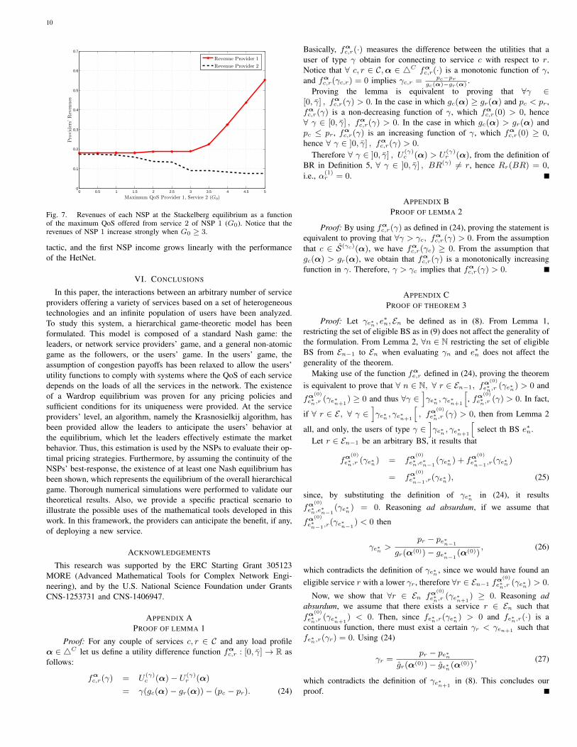
Fig. 7. Revenues of each NSP at the Stackelberg equilibrium as a functionof the maximum QoS offered from service 2 of NSP 1 (G0). Notice that therevenues of NSP 1 increase strongly when G0 ≥ 3.

tactic, and the first NSP income grows linearly with the performanceof the HetNet.

VI. CONCLUSIONS

In this paper, the interactions between an arbitrary number of serviceproviders offering a variety of services based on a set of heterogeneoustechnologies and an infinite population of users have been analyzed.To study this system, a hierarchical game-theoretic model has beenformulated. This model is composed of a standard Nash game: theleaders, or network service providers’ game, and a general non-atomicgame as the followers, or the users’ game. In the users’ game, theassumption of congestion payoffs has been relaxed to allow the users’utility functions to comply with systems where the QoS of each servicedepends on the loads of all the services in the network. The existenceof a Wardrop equilibrium was proven for any pricing policies andsufficient conditions for its uniqueness were provided. At the serviceproviders’ level, an algorithm, namely the Krasnosielkij algorithm, hasbeen provided allow the leaders to anticipate the users’ behavior atthe equilibrium, which let the leaders effectively estimate the marketbehavior. Thus, this estimation is used by the NSPs to evaluate their op-timal pricing strategies. Furthermore, by assuming the continuity of theNSPs’ best-response, the existence of at least one Nash equilibrium hasbeen shown, which represents the equilibrium of the overall hierarchicalgame. Thorough numerical simulations were performed to validate ourtheoretical results. Also, we provide a specific practical scenario toillustrate the possible uses of the mathematical tools developed in thiswork. In this framework, the providers can anticipate the benefit, if any,of deploying a new service.

ACKNOWLEDGEMENTS

This research was supported by the ERC Starting Grant 305123MORE (Advanced Mathematical Tools for Complex Network Engi-neering), and by the U.S. National Science Foundation under GrantsCNS-1253731 and CNS-1406947.

APPENDIX APROOF OF LEMMA 1

Proof: For any couple of services c, r ∈ C and any load profileα ∈ 4C let us define a utility difference function fαc,r : [0, γ]→ R asfollows:

fαc,r(γ) = U (γ)c (α)− U (γ)

r (α)

= γ(gc(α)− gr(α))− (pc − pr). (24)

Basically, fαc,r(·) measures the difference between the utilities that auser of type γ obtain for connecting to service c with respect to r.Notice that ∀ c, r ∈ C,α ∈ 4C fαc,r(·) is a monotonic function of γ,and fαc,r(γc,r) = 0 implies γc,r = pc−pr

gc(α)−gr(α).

Proving the lemma is equivalent to proving that ∀γ ∈[0, γ] , fαc,r(γ) > 0. In the case in which gc(α) ≥ gr(α) and pc < pr ,fαc,r(γ) is a non-decreasing function of γ, which fαc,r(0) > 0, hence∀ γ ∈ [0, γ] , fαc,r(γ) > 0. In the case in which gc(α) > gr(α) andpc ≤ pr , fαc,r(γ) is an increasing function of γ, which fαc,r(0) ≥ 0,hence ∀ γ ∈ ]0, γ] , fαc,r(γ) > 0.

Therefore ∀ γ ∈ ]0, γ] , U(γ)c (α) > U

(γ)r (α), from the definition of

BR in Definition 5, ∀ γ ∈ ]0, γ] , BR(γ) 6= r, hence Rr(BR) = 0,i.e., α(1)

r = 0.

APPENDIX BPROOF OF LEMMA 2

Proof: By using fαc,r(γ) as defined in (24), proving the statement isequivalent to proving that ∀γ > γc, f

αc,r(γ) > 0. From the assumption

that c ∈ S(γc)(α), we have fαc,r(γc) ≥ 0. From the assumption thatgc(α) > gr(α), we obtain that fαc,r(γ) is a monotonically increasingfunction in γ. Therefore, γ > γc implies that fαc,r(γ) > 0.

APPENDIX CPROOF OF THEOREM 3

Proof: Let γe∗n , e∗n, En be defined as in (8). From Lemma 1,

restricting the set of eligible BS as in (9) does not affect the generality ofthe formulation. From Lemma 2, ∀n ∈ N restricting the set of eligibleBS from En−1 to En when evaluating γn and e∗n does not affect thegenerality of the theorem.

Making use of the function fαe,r defined in (24), proving the theoremis equivalent to prove that ∀ n ∈ N, ∀ r ∈ En−1, f

α(0)

e∗n,r(γe∗n) > 0 and

fα(0)

e∗n,r(γe∗n+1

) ≥ 0 and thus ∀γ ∈]γe∗n , γe∗n+1

[, fα

(0)

e∗n,r(γ) > 0. In fact,

if ∀ r ∈ E , ∀ γ ∈]γe∗n , γe∗n+1

[, fα

(0)

e∗n,r(γ) > 0, then from Lemma 2

all, and only, the users of type γ ∈]γe∗n , γe∗n+1

[select th BS e∗n.

Let r ∈ En−1 be an arbitrary BS, it results that

fα(0)

e∗n,r(γe∗n) = fα

(0)

e∗n,e∗n−1

(γe∗n) + fα(0)

e∗n−1,r(γe∗n)

= fα(0)

e∗n−1,r(γe∗n), (25)

since, by substituting the definition of γe∗n in (24), it resultsfα

(0)

e∗n,e∗n−1

(γe∗n) = 0. Reasoning ad absurdum, if we assume that

fα(0)

e∗n−1,r(γe∗n−1

) < 0 then

γe∗n >pr − pe∗n−1

gr(α(0))− ge∗n−1(α(0))

, (26)

which contradicts the definition of γe∗n , since we would have found aneligible service r with a lower γr , therefore ∀r ∈ En−1 f

α(0)

e∗n,r(γe∗n) > 0.

Now, we show that ∀r ∈ En fα(0)

e∗n,r(γe∗n+1

) ≥ 0. Reasoning adabsurdum, we assume that there exists a service r ∈ En such thatfα

(0)

e∗n,r(γe∗n+1

) < 0. Then, since fe∗n,r(γe∗n) > 0 and fe∗n,r(·) is acontinuous function, there must exist a certain γr < γen+1 such thatfe∗n,r(γr) = 0. Using (24)

γr =pr − pe∗n

gr(α(0))− ge∗n(α(0)), (27)

which contradicts the definition of γe∗n+1in (8). This concludes our

proof.

11

APPENDIX DPROOF OF THEOREM 5

Proof: We begin by showing that if α∗ ∈ W then α∗ = F (α∗).We focus on an arbitrary service c ∈ C. Either this service does notbelong to any best service set, i.e., ∀ e ∈ E , c 6∈ Pe(α), or it belongsto one best service set, i.e., ∃! e : c ∈ Pe(α∗). We recall that a bestservice set is a subset of a certain same price service set, in which allservices offer the highest QoS. In the first case, since c is not into anybest service set, it is never selected by any rational user, thus, α∗c = 0.Also, following (13), Fc(α∗) = 0. Hence, for all services that do notbelong to any best service set it holds that Fc(α∗) = α∗c .

Let us consider now the case in which c is part of a best serviceset, say Pe(α∗). Let us evaluate the total load of the BS e. Knowingthat, at the WE, by Definition 3 rational users chose only to connectto a utility maximizing services, then the load equals to the sum of theloads of all the services belonging to the SPS Pe, α∗e =

∑r∈Pe α

∗r .

Since α∗ ∈ W , from (4) we have that S(γ) ⊆ S(γ)(α∗), that is allthe selected services are utility maximizing services. However, fromTheorem 3 and (10) we know that there exist two threshold, which wedenote as γe and γf , such that S(γ)(α∗) = Pe(α∗) ⇔ γ ∈ [γe, γf ].This means that all the types of user that select one of the servicesinside the SPS are in the real segment [γe, γf ], thus, the load of the BScan be calculated integrating the density function ρ(·) between thesetwo thresholds. Hence, by using the cumulative density function,

α∗e = Γ(γf )− Γ(γe). (28)

Furthermore, let all users of each type best-respond according toDefinition 5, and denote by α(1) the resulting load profile. FromTheorem 4, it results αe = Γ(γf ) − Γ(γe). Which, by using (28),allows us to say that αe = α∗e , thus αe =

∑r∈Pe α

∗r . Substituting this

in (13), we obtain Fc(α∗) = α∗c . This concludes the first part of the

proof.Next, we show the reverse implication, that is if α∗ = F (α∗) then

α∗ ∈ W . From the definition of WE in (4), we must show that thereexists a set of used services S satisfying two conditions: (i) ∀ γ ∈[0, γ] , S(γ) ⊆ S(γ)(α∗) and (ii) α∗ = R(S). Let all the users best-respond to the load α∗ according to Definition 5 and let S be one ofpossible the resulting SUS. Recall that all best-responding users of eachtype γ may select indifferently any of the services in their set of bestservices S(γ)(α∗). We want to show that S is a set of used servicewhich satisfies (i) and (ii).

Condition (i) is respected, in fact, from Definition 5, it results that∀ γ ∈ [0, γ] , S(γ) ⊆ S(γ)(α∗). That is, all the users of each typeselect a service which maximizes their utility function when the initialload profile is α∗.

To prove condition (ii), we focus on an arbitrary service c ∈ C, andwe distinguish two cases: the case in which c does not belong to anybest service set, and the case in which it belongs to a best service setdenoted by Pe(α∗). In the first case, from (13) we have that α∗c = 0.On the other hand, from Definition 8, when all user best-respond nouser select such a service, hence Rc(S) = 0, thus α∗c = Rc(S).

In the case in which c belongs to some best service set Pe(α∗),from Theorem 3, we have that there exist two unique thresholds,which we denote as γe and γf , that isolate all the users that connectto the BS e, i.e. that select one of the services belonging to thecorresponding SPS Pe. The load of the BS e, is defined as the sumof the loads of all the services belonging to Pe. Hence, after thebest-response, it is αe ,

∑r∈Pe Rr(S). On the other hand, the

assumption α∗ = F (α∗) implies, from (13), that αe =∑r∈Pe α

∗r ,

thus,∑r∈Pe Rr(S) =

∑r∈Pe α

∗r . This means that, if α∗ = F (α∗),

then, after a type wise best-response from all the users, irrespective

from the actual service chosen from all the users of any type, the sumof loads of all the services belonging to the same SPS must not change.

However, according to Definition 5, when best-responding, any usercan arbitrarily select any service belonging to the best service set.Therefore, we can select each S(γ) ∀γ ∈ [0, γ] such that Rc(S) = α∗c ,we obtain that Rc(S) = α∗c and, thus, α∗ = R(S). This concludes theproof.

APPENDIX EPROOF OF THEOREM 6

Proof: From Theorem 1, the game GF has at least one WE,that we denote by αA =

{αA0 , . . . α

AC

}and ad absurdum let

αB ={αB0 , . . . α

BC

}be a different WE, with γA =

(γA0 , . . . γ

AC

)and γB =

(γB0 , . . . γ

BC

)being the correspondent thresholds vectors.

Moreover, ∀ c ∈ C, let us denote by gAc = gc(αA) and gBc = gc(α

B)and let CA =

{0, cA1 , c

A2 , . . . c

ANA

}and CB =

{0, cB1 , c

B2 , . . . c

BNB

}be the respective strictly ordered sets of used services at the WE, thismeans that: αAc > 0 if and only if c ∈ CA and αBc > 0 if and onlyif c ∈ CB; 0 < cA1 < . . . < cANA and 0 < cB1 < . . . < cBNB with NAand NB representing the number of services used at the WE αA andαB respectively. Let us define the intersection function Iw : C2 → Ras follows:

Iw (r, s) =pr − psgwr − gws

, (29)

where r, s ∈ Cw are two arbitrary services and the superscriptw ∈ {A,B} labels the WE load profile used as the argument ofthe QoS functions. The name intersection is justified by the fact thatthe value represents the unique value of γ for which it results thatUγr (αw) = Uγs (αw), where these utility functions are defined as in (2).We underline that from Theorem 3, each threshold γAc∗n is the minimumintersection among the available services, i.e., we can write

γAc∗n = min`∈Cn−1

IA (`, c∗n−1) . (30)

In order to prove the body of the theorem, we need to introducesome preliminary results. As a first step, we show that in any WEthe first service to be used is service 0. By definition all prices arestrictly positive values, therefore ∀α ∈ W , ∀c ∈ C it results thatU0

0 (α) > U0c (α), moreover following the results of Theorem 3,

α0 = Γ(γc1), and γc1 =pc1gc1

. Since both pc1 and gc1 ∈ R+, wehave that γc1 > 0. Since Γ(·) is a strictly increasing function andΓ(0) = 0, we obtain that Γ(γc1) > 0. As a second step, we showthat if ∀` < n αA

cA`≥ αB

cB`

then ∀` ≤ n γAcA`≥ γB

cB`

. We proceed byinduction on n defining the following proposition

O` : αAcA`≥ αBcB

`⇒ γAcA

`+1≥ γBcB

`+1. (31)

We show that for ` = 1O` is true. Considering that Γ(0) = 0, from (11)we have that αA0 ≥ αB0 implies Γ

(γAcA1

)≥ Γ

(γBcB1

). By definition,

Γ(·) is a monotonically increasing function, hence γAcA1≥ γB

cB1. To

complete the proof, let us assume O` to be true ∀` < n andprove that On is also true. From (11) αAcAn

≥ αBcBnimplies that

Γ(γAcAn+1

)− Γ

(γAcAn

)≥ Γ

(γBcBn+1

)− Γ

(γBcBn

)which can be written

as Γ(γAcAn+1

)− Γ

(γBcBn+1

)≥ Γ

(γAcAn

)− Γ

(γBcBn

). Since On−1 is

true we have that γAcAn ≥ γBcBn, which means Γ

(γAcAn

)≥ Γ

(γBcBn

),

since Γ(·) is monotonically increasing. Therefore, we can write thatΓ(γAcAn+1

)− Γ

(γBcBn+1

)≥ 0, thus, γA

cAn+1≥ γB

cBn+1which proves On.

In the following we prove the main body of the theorem. With noloss of generality, let us assume αA0 ≥ αB0 . We aim at proving thatif αA0 ≥ αB0 then ∀ ` ∈ C αA` ≥ αB` which, since αA,αB ∈ 4Cand αA 6= αB is absurd. Let us recall that the services are organized

12

price wise in an increasing order and that prices do not change fromαA to αB . For an arbitrary service n ∈ C either n ∈ CB or n 6∈ CB.If n 6∈ CB, then αBn = 0, thus αBn ≤ αAn . As a consequence we focusonly on the services which belong to CB. We proceed by induction. Letus define the proposition P` :

αA` ≥ αB` , if ` ∈ CA ∩ CB then gA` ≤ gB` . (32)

It is easy to show that P0 is true, since we assumed that αA0 ≥ αB0 ,and from the definition of service 0 we have that gA0 = gB0 = 0. Tocomplete the proof, let us assume P` to be true ∀` ∈ C, ` < n, and letus show that Pn is true.

If n 6∈ CB then αBn = 0 thus αBn ≤ αAn which prove the thesis. Ifn ∈ CB then αBn > 0, thus proving that

gBn ≥ gAn (33)

is sufficient to prove the thesis, since from H1 (33) implies αAn ≥ αBn ,which implies αAn > 0 thus n ∈ CA.

To simplify the notation, let us denote the two sets of used service atthe two WE as follows: CA = {. . . b, r . . .} and CB = {. . . b, n, . . .}.Here, b is the service used before n in the WE αB (i.e., b =max

{` ∈ CB|` < n

}) and r is the service used in the WE αA just

after b (i.e., r = min{` ∈ CA|` > b

}). Notice that, from (32), b ∈ CB

and b < n imply that b ∈ CA. Moreover, n might belong or not to CA,thus, we denote the service successive to b in αA by r. From (31), wehave that γAr ≥ γBn , which can be expressed by using the function (29)as IA(r, b) ≥ IB(n, b). Also, since r ∈ CA we have from Theorem 3that either gAn ≤ gAb or IA(r, b) < IA(n, b). We analyze the two casesseparately.

The first case is absurd. If gAn ≤ gAb then n 6∈ CA, αAn = 0, thusn ∈ CB implies αAn < αBn which from assumption H1 implies gBn ≤gAn . Moreover, b ∈ CB implies that αBb > 0 thus, from assumption(32), αAb > 0 and b ∈ CA, which, from assumption (32) insures thatgAb ≤ gBb . Reconstructing the chain of inequalities, we obtain gBn ≤ gBb ,that, from Lemma 2 implies n 6∈ CB, which is absurd.

In the second case, we have that gAn > gAb and IA(n, b) > IA(r, b).As we have already stated, (31) implies that IA(r, b) > IB(n, b), hencewe obtain IA(n, b) > IB(n, b), thus

pn − pbgAn − gAb

>pn − pbgBn − gBb

,

gBn − gBb > gAn − gAb ,gBn − gAn > gBb − gAb , (34)

where both parts of the first inequality are positive since from n ∈ CBwe have that gBn − gBb > 0 and n > b implies pn > pb. Notice thatb ∈ CB implies that αBb > 0, thus, since b < n assumption (32) impliesthat αAb > 0 and b ∈ CA, which, from assumption (32) insures thatgBb > gAb . This, from (34) gives gBn > gAn .

APPENDIX FPROOF OF THEOREM 7

Proof: Let us consider two different load profiles αA =(αA0 , . . . , α

AC

)and αB =

(αB0 , . . . , α

BC

)and let us assume αA0 ≥ αB0 .

Any QoS function respecting conditions (i)− (iv) can be written as

gc (α) = fc(αc) +mc

∑`∈C\{0,c}

α`, (35)

where fc : [0, 1] → R is a function such that ∂gc∂αc

= dfcdαc

. Then, forany arbitrary service c ∈ C \ {0} it results that:

gc(αA) = gc(α

B) + fc(αAc )− fc(αBc ) +mc

∑`∈C\{0,c}

(αA` − αB`

).

(36)

If αAc ≤ αBc , then from the fundamental Theorem of calculus fc(αBc )−fc(α

Ac ) < mc

(αBc − αAc

), thus

fc(αAc )− fc(αBc ) > mc

(αAc − αBc

). (37)

From (36) we can write:

gc(αA) >gc(α

B) +mc

(αAc − αBc

)+mc

∑`∈C\{0,c}

(αA` − αB`

)(38)

=gc(αB) +mc

∑`∈C\{0}

(αA`

)−

∑`∈C\{0}

(αB`

) (39)

=gc(αB) +mc

(αB0 − αA0

)(40)

>gc(αB), (41)

where the passage between (39) and (40) is justified by the fact that∀α ∈ 4C it results

∑`∈C\{0} α` = 1− α0, and the passage between

(40) and (41) is justified from the assumptions that αA0 ≥ αB0 andmc ≤ 0.

If gc(αA)≤ gc

(αB)

then from (36) we have

fc(αAc )− fc(αBc ) +mc

∑`∈C\{0,c}

(αA` − αB`

)< 0

fc(αAc )− fc(αBc )−mc

(αAc − αBC

)< −mc

(αB0 − αA0

). (42)

From the assumptions that mc ≤ 0 and αA0 ≤ αB0 , we have thatfc(α

Ac ) − fc(αBc ) − mc

(αAc − αBC

)≤ 0, i.e. fc(αAc ) − fc(αBc ) ≤

mc

(αAc − αBC

), which from assumption (iii) and the fundamental

Theorem of calculus, is true if αAc > αBc and, from (37), is falseif αAc ≤ αBc . Therefore, we have proven that if αAc ≤ αBc , thengc(α

A) ≥ gc(αB) and if gc(αA) ≤ gc(α

B), then αAc ≥ αBc , hencefrom Theorem 6 the game GF admits only one equilibrium.

APPENDIX GPROOF OF THEOREM 8

Proof: Let us begin by distinguishing two cases: (i)∃ limn→∞α

(n); (ii) @ limn→∞α(n). In the first case, Banach

fixed-point theorem, and the continuity of F (·) guarantee thatlimn→∞α

(n) = α∗. Indeed, if F (·) is continuous then also G(·) iscontinuous, since is a composition of continuous functions. Let usdenote as e the converging point, that is: limn→∞α

(n) = e, therefore,we have:

limn→∞

α(n) = limn→∞

G(α(n−1)) (43)

= G( limn→∞

α(n−1)) = G(e). (44)

The passage from (43) and (44) is giustfied by the continuity of G(·).Since, by definition, limn→∞α

(n) = e we have e = G(e) which meansthat e is a fixed-point of G(·) and, thus, of F (·). Therefore, if thereexists a limit, (i.e., if the algorithm converges) it converges to a fixedpoint. Notice that, the existence of the limit can also be expressed as:∃α∗ ∈ W : limn→∞||α−α∗|| = 0. In the second case, let us definea distance sequence as

dn = ||α(n) −α∗||. (45)

The thesis, thus, amounts to prove that ∃N : ∀n > N, dn ≤ λK2C

. Wedivide the proof in two steps: first, we prove that ∃N : dN ≤ λK( 1

2ζ),

second, by using Lemma 5, we show that ∀n > N dn ≤ λK( 12ζ

+ 1).Notice that:• with no loss of generality, we assume α(0) to be any α ∈ A such

that d0 > λK( 12ζ

), since otherwise the thesis results immediatelyproven,

13

• dn >λK2ζ

implies, from Theorem 9, dn+1 < dn, i.e., ∀n : dn >λK2ζ, the sequence {dn} is monotonically decreasing.

We shall prove that ∃N : dN ≤ λK2ζ

reasoning ad absurdum. Let us,thus, assume that @N : dN ≤ λK

2ζ, then {dn}∞0 is a monotonically

decreasing sequence, hence it has a limit. That is limn→∞dn = d,which we assume to be d > λK

2ζ. We recall that for (63) and Lemma

3, we have that

||G(α)−α∗||2 =||α−α∗||2 + ||G(α)−α|| (||G(α)−α|| − 2ζ||α−α∗||) ,

(46)thus, by using α(n) = G(α(n−1)), dn = ||α(n) − α∗|| and definingan = ||G(α(n−1))−α(n−1)|| we can write

d2n = d2

n−1 + an (an − 2ζdn−1) . (47)

The sequence an is bounded, since 0 < an ≤ λK. Thus, from theBolzano-Weierstrass theorem there exists a subsequence of an whichconverges inside the boundaries. That is ∃ {bk}∞0 ∈ N : bk+1 >bk, limk→∞ abk = a, a ∈ [0, λK]. Moreover Proposition 1.4.12 in[27] insures that all the subsequences of a convergent sequence convergeto the same limit, which means limk→∞dbk = d. We can then write(47) as:

d2bk = d2

bk−1 + abk (abk − 2ζdbk−1) , (48)

and passing at the limit, we get d2 = d2 + a (a− 2ζd) . This impliesthat, either a − 2ζd = 0 or a = 0. In the first case, we would haved = a

2ζ, and since a ≤ λK then we have d ≤ λK

2ζwhich contradicts the

assumption that d > λK2ζ

. If a = 0, this means limk→∞||G(α(bk)) −α(bk)|| = 0. This means limk→∞α

(bk) ∈ W , thus the algorithm hasconverged to a fixed point which contradicts the assumptions.

APPENDIX HPROOF OF THEOREM 9

In order to prove this Theorem, we first show some useful Lemmas.

Lemma 3 Let G(·) be such that G(α) = (1 − λ)α + λF (α), thenG(α)−α = λ (F (α)−α))

Proof: By substituting (16) in G(α)−α, we have :

G(α)−α = ((1− λ)α+ λF (α)−α) (49)

= λ(F (α)−α). (50)

Lemma 4 Let us assume that ∀α ∈ 4C F (·) is such that

||F (α)−α∗||2 < ||F (α)−α||2 + ||α−α∗||2, (51)

then, it results that

||G(α)−α∗||2 < ||G(α)−α||2 + ||α−α∗||2, (52)

Proof: Assumption (17) is equivalent to〈(F (α)−α) , (α−α∗)〉 < 0, since we can write||F (α) − α∗||2 = ||(F (α) − α) + (α − α∗)||2 and, from thepolarization identity 7

||(F (α)−α) + (α−α∗)||2 =||F (α)−α||2 + ||α−α∗||2 + 2 〈(F (α)−α) , (α−α∗)〉 .

(53)7Let x,y be ∈ V two vector on a vectorial space V on which it has been defined

a scalar product 〈·, ·〉, then we have that ||x+y||2 = ||x||2+||y||2+2< (〈x, y〉).Since in our case α, F (α) ∈ 4S ⊂ RS , 2< (〈x, y〉) = 2〈x, y〉.

For Lemma 3 and the inner product definition (left multiplication by ascalar), we have that

〈(F (α)−α) , (α−α∗)〉 =1

λ〈(G(α)−α) , (α−α∗)〉 . (54)

Thus, we have that 〈(G(α)−α) , (α−α∗)〉 < 0. Writing ||G(α) −α∗||2 as ||G(α)−α∗||2 = ||(G(α)−α) + (α−α∗)||2 we apply thepolarization identity and, using the previous result, we obtain

||(G(α)−α∗)||2 = ||G(α)−α||2 + ||α−α∗||2 + (55)

2 〈(G(α)−α) , (α−α∗)〉 (56)

< ||G(α)−α||2 + ||α−α∗||2. (57)

This ends our proof.

Lemma 5 For all α ∈ 4C we have that

||G(α)−α∗|| ≤ ||α−α∗||+ λK. (58)

Proof: We can write ||G(α) − α∗|| = ||G(α) − α + α − α∗||,then for the triangular inequality, we have that

||G(α)−α+α−α∗|| ≤ ||G(α)−α||+ ||α−α∗||. (59)

Since ||G(α) − α|| = λ||F (α) − α|| from Lemma 3, and from thedefinition of K we have that

||G(α)−α||+ ||α−α∗|| ≤ λK + ||α−α∗||. (60)

Hereunder, we show the proof of the Theorem.Proof: We begin by rewriting the distance between a single iteration

of the Krasnosielkij algorithm and a fixed point α∗ as follows: ||G(α)−α∗||2 = ||(G(α)−α)+(α−α∗)||2. Thus, by means of the polarizationidentity and the properties of the inner product, we can write

||G(α)−α∗||2 = ||G(α)−α||2 + ||α−α∗||2++2 cos(θ)||G(α)−α||||α−α∗||. (61)

Here, θ is the angle between the two vectors G(α)−α and α−α∗.The assumption that ||F (α)−α∗||2 < ||F (α)−α||2 +||α−α∗||2 andLemma 4 guarantee that ||G(α)−α∗||2 < ||G(α)−α||2+||α−α∗||2,which implies 2 cos(θ)||G(α) − α||||α − α∗|| < 0. Since the normscannot obtain negative values, it means that cos(θ) < 0. For simplicity,we introduce a positive constant C = − cos(θ), thus 0 < C ≤ 1.Therefore, using Lemma 3, we can write (61) as

||G(α)−α∗||2 = ||F (α)−α||2λ2 + ||α−α∗||2 + (62)

−2Cλ||F (α)−α||||α−α∗||

With some algebra, and by using the assumption that ||α−α∗|| ≥ λ K2C

we can write:

||G(α)−α∗||2 == ||α−α∗||2 + λ||F (α)−α|| (λ||F (α)−α|| − 2C||α−α∗||)≤ ||α−α∗||2 + λ||F (α)−α|| (λK − 2C||α−α∗||)≤ ||α−α∗||2 + λ||F (α)−α|| (λK − λK)= ||α−α∗||2.

(63)Notice that the passage is justified from the fact that ||F (α)−α||λ ≥ 0∀α. Moreover, since by definition both ||G(α)−α∗|| and ||α−α∗|| arenon-negative, ||G(α)−α∗||2 ≤ ||α−α∗||2 implies ||G(α)−α∗|| ≤||α−α∗||.

14

APPENDIX ISKETCH OF THE PROOF OF CONJECTURE 1

Proof: It is possible express the equilibrium as the result of asufficient number of iterations of (16), that is α∗(p) = α(T ), where Tis a large enough number of iterations.

Let us define γ(t) as the thresholds vector underlying the t-th iterationof the Krasnosielkij algorithm α(t).

For any arbitrary α(t−1), Theorem 3 implies that any arbitrary n-th element of γ(1) is expressed from (8), more precisely γ

(t)c∗n

=(pc∗n−pc∗

n−1

gc∗n(α(t−1))−gc∗

n−1(α(t−1))

)which is a continuous function of any

price vector. Furthermore, the function Γ(·) is continuous, being anintegral function. Hence, ∀ e ∈ E , α(t)

e = Γ(γf )−Γ(γe) is continuousw.r.t. the pricing vector. Hence, ∀ t ∈ N

α(t)(p) = limp→p

α(t)(p). (64)

REFERENCES

[1] C. V. N. Index, “Global mobile data traffic forecast update, 2010-2015,”Cisco white paper, 2011.

[2] R. Q. Hu, Y. Qian, S. Kota, and G. Giambene, “Hetnets-a new paradigm forincreasing cellular capacity and coverage,” IEEE transaction on WirelessCommunications, vol. 18, no. 3, pp. 8–9, 2011.

[3] T. Q. S. Quek, G. de la Roche, I. Guvenc, and M. Kountouris. CambridgeUniversity Press, Apr. 2013.

[4] J. Hoydis, M. Kobayashi, and M. Debbah, “Green small-cell networks,”Vehicular Technology Magazine, IEEE, vol. 6, no. 1, pp. 37 –43, march2011.

[5] J. D. Hobby and H. Claussen, “Deployment options for femtocells and theirimpact on existing macrocellular networks,” Bell Labs Technical Journal,vol. 13, no. 4, pp. 145–160, 2009.

[6] W. Webb, Wireless communications: The future. Wiley, 2007.[7] Z. Hasan, H. Boostanimehr, and V. K. Bhargava, “Green cellular networks:

A survey, some research issues and challenges,” IEEE CommunicationsSurveys & Tutorials, vol. 13, no. 4, pp. 524–540, May 2011.

[8] N. Shetty, S. Parekh, and J. Walrand, “Economics of femtocells,” in Proc.of IEEE GLOBECOM, Hawaii, USA, Nov. 2009.

[9] S. Ren and M. van der Schaar, “Data demand dynamics in wireless com-munications markets,” IEEE Transactions on Signal Processing, vol. 60,no. 4, pp. 1986–2000, 2012.

[10] S. Ren, J. Park, and M. van der Schaar, “User subscription dynamics andrevenue maximization in communications markets,” in IEEE INFOCOM,Shanghai, China, Apr. 2011, pp. 2696–2704.

[11] ——, “Entry and spectrum sharing scheme selection in femtocell commu-nications markets,” IEEE Transaction on Networking, vol. 21, no. 1, pp.218 –232, Feb. 2013.

[12] N. Nisan, T. Roughgarden, E. Tardos, and V. V. Vazirani, Algorithmic GameTheory. New York, NY, USA: Cambridge University Press, 2007.

[13] C. Gussen, E. Belmega, and M. Debbah, “Pricing and bandwidth allocationproblems in wireless multi-tier networks,” in Proc. of IEEE Asilomar Conf.on Signals, Systems, and Computers, Pacific Grove, USA, Nov. 2011.

[14] L. Rose, E. Belmega, W. Saad, and M. Debbah, “Dynamic service selectiongames in heterogeneous small cell networks with multiple providers,” Paris,France, Aug. 2012, pp. 1078–1082.

[15] H. von Stackelberg, The theory of the market economy. Oxford, England:Oxford Univ. Press, 1952.

[16] T. Roughgarden and E. Tardos, “How bad is selfish routing?” Journal ofthe ACM (JACM), vol. 49, no. 2, pp. 236–259, 2002.

[17] I. Milchtaich, “Generic uniqueness of equilibrium in large crowdinggames,” Journal of Mathematics of Operations Research, vol. 25, no. 3,pp. 349–364, 2000.

[18] A. Haurie and P. Marcotte, “On the relationship between Nash-Cournot andwardrop equilibria,” Networks, vol. 15, no. 3, pp. 295–308, 1985.

[19] J. G. Wardrop, “Some theoretical aspects of road traffic research,” Proc. ofInstitute of Civil Engineers, Part II, vol. 1, pp. 325–378, 1952.

[20] M. Smith, “The existence, uniqueness and stability of traffic equilibria,”Transportation Research Part B: Methodological, vol. 13, no. 4, pp. 295–304, 1979.

[21] D. Schmeidler, “Equilibrium points of nonatomic games,” Journal of Stat.Phys., vol. 7, no. 4, pp. 295–300, 1973.

[22] D. Fudenberg and J. Tirole, Game Theory. Cambridge, MA, USA: MITPress, 1991.

[23] V. Berinde, Iterative approximation of fixed points, 2nd edition. Springer,2007.

[24] J. W. Weibull, Evolutionary Game Theory, 1995.[25] L. E. J. Brouwer, “Uber abbildung von mannigfaltigkeiten,” Mathematische

Annalen, vol. 71, no. 1, pp. 97–115, 1911.[26] D. Fudenberg and D. K. Levine, The Theory of Learning in Games, ser.

MIT Press Books. The MIT Press, 1998, vol. 1.[27] K. Prakash, Y. K. Goyal, and R. Bhalla, BCA Mathematics 103. Laxmi

Publications, Ltd., 2010.

Luca Rose (S’10 M’14) was born in Pisa, Italy. Hereceived his B.Sc. degree in telecommunications en-gineering from the University of Pisa, Italy. In 2009he received his M.Sc. degree with honours from thesame university. From 2010 to 2013, he has beenattending his PhD studies on Game theory and Learningtheory as a member of the Alcatel-Lucent chair inflexible radio in Supelec, sponsored by Thales Com-munications & Security, in the context of the projectCORASMA (COgnitive RAdio for dynamic SpectrumMAnagement). Since 2014 he is a researcher in themathematics and algorithms design lab of the Huawei

french research center, in Boulogne-Billancourt, France. His research interestsspan from the field of software defined radio to the field of Game theory andLearning theory, small cells, M2M communications, and distributed resourceallocation.

E. Veronica Belmega (S’07, M’10) was born in Fa-garas, Romania. She received the B.Sc. degree fromthe University Politehnica of Bucharest, Romania, in2007. She obtained the M.Sc. and Ph.D. degrees, bothfrom the Universite Paris-Sud 11, Paris, France, in2007 and 2010 respectively. In 2010-2011, she was apost-doctoral researcher in a joint project between theAlcatel-Lucent Chair on Flexible Radio in Supelec andPrinceton University. She is currently an associate pro-fessor at ETIS/ENSEA-Universite de Cergy-PontoiseCNRS, Cergy-Pontoise, France. She was one of theten recipients of the 2009 L’Oreal UNESCO French

Academy of Science Fellowship: ”For young women doctoral candidates inscience”.

Walid Saad (S’07, M’10) received his B.E. degree inComputer and Communications Engineering from theLebanese University, in 2004, his M.E. in Computerand Communications Engineering from the AmericanUniversity of Beirut (AUB) in 2007, and his Ph.Ddegree from the University of Oslo in 2010. StartingAugust 2014, he is an Assistant Professor at the Elec-trical and Computer Engineering Department at Vir-ginia Polytechnic Institute and State University. Priorto joining VT, he was an Assistant Professor at theElectrical and Computer Engineering Department atthe University of Miami (08/11 - 08/14) and he has

held several research positions at institutions such as Princeton University andthe University of Illinois at Urbana-Champaign. His research interests includewireless and small cell networks, game theory, smart grid, network science,cognitive radio, wireless security, and self-organizing networks. He has co-authored one book and over 95 international conference and journal publicationsin these areas. Dr. Saad is the recipient of the NSF CAREER award in 2013.He was the author/co-author of the papers that received the Best Paper Awardat the 7th International Symposium on Modeling and Optimization in Mobile,Ad Hoc and Wireless Networks (WiOpt), in June 2009, at the 5th InternationalConference on Internet Monitoring and Protection (ICIMP) in May 2010, andat the IEEE Wireless Communications and Networking Conference (WCNC) in2012.

Merouane Debbah (SM’08) entered the Ecole Nor-male Superieure de Cachan (France) in 1996 where hereceived his M.Sc and Ph.D. degrees respectively. Heworked for Motorola Labs (Saclay, France) from 1999-2002 and the Vienna Research Center for Telecommu-nications (Vienna, Austria) until 2003. He then joinedthe Mobile Communications department of the InstitutEurecom (Sophia Antipolis, France) as an AssistantProfessor until 2007. He is now a Full Professor atSupelec (Gif-sur-Yvette, France), holder of the Alcatel-Lucent Chair on Flexible Radio and a recipient of theERC starting grant MORE (Advanced Mathematical

Tools for Complex Network Engineering). His research interests are in infor-mation theory, signal processing and wireless communications. He is a seniorarea editor for IEEE Transactions on Signal Processing and an Associate Editorin Chief of the journal Random Matrix: Theory and Applications. MerouaneDebbah is the recipient of the ”Mario Boella” award in 2005, the 2007 GeneralSymposium IEEE GLOBECOM best paper award, the Wi-Opt 2009 best paperaward, the 2010 Newcom++ best paper award, the WUN CogCom Best Paper2012 and 2013 Award as well as the Valuetools 2007, Valuetools 2008, Valuetools2012 and CrownCom2009 best student paper awards. He is a WWRF fellow andan elected member of the academic senate of Paris-Saclay. In 2011, he receivedthe IEEE Glavieux Prize Award. He is the co-founder of Ximinds.