pricing hydroelectric power plants with/without ...paforsyt/powerplant.pdf · pricing hydroelectric...

Pricing Hydroelectric Power Plants with/withoutOperational Restrictions: a Stochastic Control Approach

Zhuliang Chen1, Peter A. Forsyth2

1 David R. Cheriton School of Computer Science, University of Waterloo, Waterloo, ON, Canada N2L 3G12 David R. Cheriton School of Computer Science, University of Waterloo, Waterloo ON, Canada N2L 3G1

Abstract. In this paper, we value hydroelectric power plant cash flows under a stochastic con-trol framework, taking into consideration the implication of operational constraints such as rampingand minimum flow rate constraints for the purpose of environmental protection. The power plantvaluation problem under a ramping constraint is characterized as a bounded stochastic control prob-lem, resulting in a Hamilton-Jacobi-Bellman (HJB) partial integrodifferential equation (PIDE). Thevaluation problem without the ramping restriction is characterized as an unbounded stochastic con-trol problem; we propose an impulse control formulation, resulting in an HJB variational inequality,for the valuation problem under this scenario. We develop a consistent numerical scheme for solv-ing both the HJB PIDE for the bounded control problem and the HJB variational inequality for theunbounded control problem. We prove the convergence of the numerical scheme to the viscositysolution of each pricing equation, provided a strong comparison result holds. Numerical resultsindicate that failing to consider operational constraints may considerably overestimate the value ofhydroelectric power plant cashflows.

1 Introduction

A hydroelectric power plant generates electricity by releasing water from a reservoirthrough the turbine located downstream of the dam. The electricity power produced re-lies on the rate of water flowing through the turbine, which is controlled by the rampingrate (the rate of change of flow through the turbine) chosen by the operator. In order to gainprofits, the operator of a hydroelectric power plant must determine the appropriate rampingrate in response to stochastic electricity prices. Furthermore, the operator is required toconform to various operational restrictions, such as ramping and minimum flow rate con-straints, imposed by the government for the purpose of environmental protection [14]. Thevaluation of hydroelectric power plants is characterized as a stochastic control problem withthe ramping rate (which can be either bounded or unbounded) as the control variable.

In this paper, we focus on valuing hydroelectric power plant cash flows by solving thecorresponding stochastic control problem, and studying the implication of the operationalconstraints on the value of power plants.

Following [7, 8, 24], we can formulate the hydroelectric power plant pricing problem(i.e., the stochastic control problem) as a Hamilton-Jacobi-Bellman (HJB) partial integrod-

1

2 Zhuliang Chen, Peter A. Forsyth

ifferential equation (PIDE) and an HJB variational inequality respectively for the cases withand without a ramping constraint. Then we can use PDE based approaches to solve the HJBequation/variational inequality numerically.

In general, the solution to an HJB equation/variational inequality may not be unique.According to [15, 23], the viscosity solution to the HJB equation/variational inequality isnormally identical to the value of the corresponding stochastic control problem. There-fore, as noted in [2, 16], it is important to ensure that a numerical scheme converges to theviscosity solution of the equation, which is the appropriate solution of the correspondingstochastic control problem.

Based on the work in [7,8], we develop a consistent numerical scheme to solve both theHJB equation and the HJB variational inequality. In both cases, the numerical techniquecan be shown to converge to the viscosity solution of the pricing equation. Our main resultsare the following:

• We propose an HJB PIDE for the valuation of a hydroelectric power plant under aramping constraint. We use a one-factor model for the electricity spot price that isable to capture major features of electricity prices such as mean-reverting dynamics,daily price trends, and price spikes.

• We present a semi-Lagrangian scheme, based on the scheme proposed in [8], to solvethe HJB PIDE. The timestepping scheme is an implicit-explicit scheme with the inte-gral terms treated explicitly. As discussed in [12], this scheme is unconditionally sta-ble. The two integral terms in the PIDE are evaluated using a Fast Fourier Transform(FFT). Provided a strong comparison result holds, we prove the scheme converges tothe unique viscosity solution of the pricing PIDE.

• We also consider a scenario with no ramping constraint. Formally, this case canbe considered to be the limit obtained by allowing the ramping rate to become un-bounded. We propose an impulse control formulation for this situation, resulting inan HJB variational inequality.

• We derive a simple extension of the the discretization scheme for the HJB PIDE underramping constraints to solve the HJB variational inequality with unbounded rampingrates. Provided a strong comparison result holds, we prove the scheme converges tothe unique viscosity solution of the HJB variational inequality.

• We study the implication of operational restrictions on the optimal control strategiesand the value of the power plant. Through an example, our numerical results in-dicate that the operational constraints can reduce the value of the power plant cashflows by more than 37% compared to the case with no ramping constraints and nominimum flow requirements. Therefore, it is important to take these constraints intoconsideration in order to accurately value the plant revenues.

Pricing Hydroelectric Power Plants with/without Operational Restrictions: a StochasticControl Approach 3

1.1 Previous work

Pricing and scheduling hydroelectric and thermal power generation assets is a popular re-search topic (see, e.g., [14, 18, 19, 21, 24] for the work on hydroelectric power generatorsand [10, 24, 25, 28] for the research on thermal power generators).

The authors of [14, 18, 19] study the short-term scheduling of hydroelectric power gen-eration systems with various operational constraints including a ramping constraint. Theirresearch focuses on scheduling a number of power systems under the assumption of knownelectricity prices with the main effort placed on solving nonlinear optimization problems,while in this paper we consider the operation of a single power plant under electricity priceuncertainty.

The authors of [21] consider the long and medium term production planning of a hy-dropower system under price and inflow uncertainty. However, they assume a parametricform for the control strategies in order to solve the valuation problem. As such, the resultingcontrol strategies may not be optimal, and hence the method tends to undervalue the powersystem. Furthermore, no operational constraints are considered in [21].

The research in [24] focuses on the value of a pump-storage facility in the PDE frame-work. The pump storage facility allows water to be pumped to the reservoir when theelectricity price is low and to be released from the storage to generate electricity when theelectricity price is high, and thus resulting in profit. Their work, however, does not consideroperational constraints. Moreover, the pricing equation is solved numerically using an ex-plicit finite differencing method, which is known to suffer from timestep restrictions due tostability considerations.

2 Hydroelectric Power Plant Valuation Problem

This section defines the short-term hydroelectric power plant valuation problem and pro-poses the pricing equations for the value of a hydroelectric power plant. The section isarranged as follows: first, we define some notation for the problem; we then present a one-factor model for electricity spot prices that is able to capture main features of the marketelectricity prices. Based on the spot price model, we propose two pricing equations for theproblem: one incorporates the regulatory operational constraints, the other does not. Wealso provide the boundary conditions for the pricing equations to completely specify thehydroelectric power plant valuation problem.

2.1 Problem notation

We use the following notation for the hydroelectric power plant valuation problem:

• t: time in hours.

• P : current electricity spot price.


• h: head of the water above the turbine (i.e., the difference in elevation between waterlevels upstream and downstream of a dam). We assume that h can be any value lyingwithin the domain [hmin, hmax], where hmin, hmax are positive constants specified inthe management plan.

• c: rate of the water flowing through the turbine (outflow rate). We assume c canbe any value residing within the domain [cmin, cmax], where cmin ≥ 0 and cmax isdetermined by the turbine’s head due to Bernoulli’s law [24]. For a hydroelectricpower plant, the change on the head is usually much smaller (e.g., within meters)compared with the head itself (e.g., a hundred meters). As a result, instead of treatingcmax as a function of the head h, in this paper, we regard cmax as a positive constant.

• T : Cash flow horizon. We will typically choose T = 1 week. This will determinethe risk neutral revenues obtained through optimal operation of the plant in a typicalweekly cycle.

• V (P, c, h, τ): value of the hydroelectric power plant as a function of electricity priceP , outflow rate c, head h and current time to the cash flow horizon τ = T − t, wheret denotes the current time.

• z: control variable that represents the ramping rate imposed by the power plant. Thatis, we have

dc

dt= z. (2.1)

According to equation (2.1), z > 0 represents ramp-up (i.e., increasing the outflowrate c), z < 0 represents ramp-down (i.e., decreasing the outflow rate c), while z = 0represents keeping the current outflow rate unchanged.

• f : rate of the water flowing into the dam (inflow rate). In this paper, we assume that fis a positive constant. It is straightforward to extend f to be a deterministic functionof t or to follow a stochastic process [24].

• a: surface area of the hydroelectric reservoir. We assume that the volume of thereservoir is a · h, where h is the depth of the reservoir.

• H(c, h): amount of power produced by the power generator as a function of outflowrate c and head h. According to [24], in theory, the power generated by a hydroelectricpower plant is given by

Hm(c, h) = gρch, (2.2)

where g is the acceleration of gravity, ρ is the density of water. Let η(c, h) be anonlinear function of c and h representing the efficiency of the turbine. Then theactual power generated by the turbine is represented by

H(c, h) = Hm(c, h)η(c, h). (2.3)


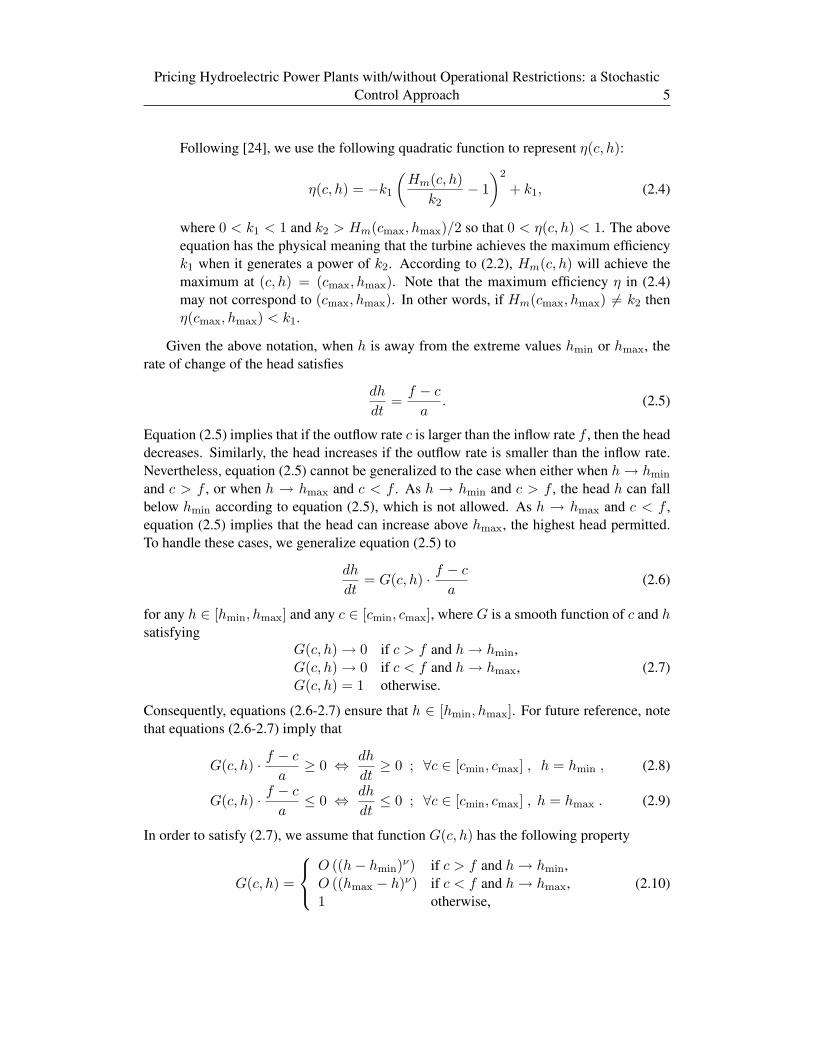
Following [24], we use the following quadratic function to represent η(c, h):

η(c, h) = −k1

(Hm(c, h)

k2− 1

)2

+ k1, (2.4)

where 0 < k1 < 1 and k2 > Hm(cmax, hmax)/2 so that 0 < η(c, h) < 1. The aboveequation has the physical meaning that the turbine achieves the maximum efficiencyk1 when it generates a power of k2. According to (2.2), Hm(c, h) will achieve themaximum at (c, h) = (cmax, hmax). Note that the maximum efficiency η in (2.4)may not correspond to (cmax, hmax). In other words, if Hm(cmax, hmax) 6= k2 thenη(cmax, hmax) < k1.

Given the above notation, when h is away from the extreme values hmin or hmax, therate of change of the head satisfies

dh

dt=f − c

a. (2.5)

Equation (2.5) implies that if the outflow rate c is larger than the inflow rate f , then the headdecreases. Similarly, the head increases if the outflow rate is smaller than the inflow rate.Nevertheless, equation (2.5) cannot be generalized to the case when either when h→ hmin

and c > f , or when h → hmax and c < f . As h → hmin and c > f , the head h can fallbelow hmin according to equation (2.5), which is not allowed. As h → hmax and c < f ,equation (2.5) implies that the head can increase above hmax, the highest head permitted.To handle these cases, we generalize equation (2.5) to

dh

dt= G(c, h) · f − c

a(2.6)

for any h ∈ [hmin, hmax] and any c ∈ [cmin, cmax], where G is a smooth function of c and hsatisfying

G(c, h) → 0 if c > f and h→ hmin,G(c, h) → 0 if c < f and h→ hmax,G(c, h) = 1 otherwise.

(2.7)

Consequently, equations (2.6-2.7) ensure that h ∈ [hmin, hmax]. For future reference, notethat equations (2.6-2.7) imply that

G(c, h) · f − c

a≥ 0 ⇔ dh

dt≥ 0 ; ∀c ∈ [cmin, cmax] , h = hmin , (2.8)

G(c, h) · f − c

a≤ 0 ⇔ dh

dt≤ 0 ; ∀c ∈ [cmin, cmax] , h = hmax . (2.9)

In order to satisfy (2.7), we assume that function G(c, h) has the following property

G(c, h) =

O ((h− hmin)ν) if c > f and h→ hmin,O ((hmax − h)ν) if c < f and h→ hmax,1 otherwise,

(2.10)


where ν is any small positive constant.As outflow rate c→ cmin, condition

dc

dt≥ 0 (2.11)

needs to be satisfied so that the outflow rate does not decrease below the minimum flow ratecmin. Similarly, condition

dc

dt≤ 0 (2.12)

must be satisfied when c → cmax so that the outflow rate does not increase above themaximum flow rate cmax. From equations (2.1) and (2.11-2.12), the above analysis resultsin the following conditions on the ramping rate z:

z ≥ 0 , c = cmin, (2.13)

z ≤ 0 , c = cmax. (2.14)

In order to satisfy conditions (2.13-2.14), we will further assume that

minz = O((c− cmin)θ

), if c→ cmin, (2.15)

maxz = O((cmax − c)θ

), if c→ cmax, (2.16)

where θ is any positive constant. Condition (2.15) has the physical meaning that the op-erator of the power plant has to gradually decrease the maximum ramp-down rate min(z)towards zero when c is close to cmin, instead of suddenly switching it to zero at c = cmin.A similar explanation applies to the condition (2.16).

In the following, we only require that θ, ν > 0. If θ 1, then according to (2.15-2.16),for all practical purposes, the operator can switch ramping rates virtually instantaneously tozero at cmin and cmax. If ν 1, then (2.7) implies that the change of head can be reducedto zero virtually instantaneously at hmin and hmax. We require θ, ν > 0 to simplify someof the proofs in subsequent sections.

At a point (P, c, h), the rate of cash flow (instantaneous revenue) received by the op-erator of the power plant is H(c, h) · P , obtained from selling the generated electricity tothe spot market at price P . Similar to the above analysis, we need to pay attention to twocases when h → hmin, c > f and h → hmax, c < f . Since these two cases can result inpotential decrease/increase of the head below/above the lower/upper bound, we will imposea penalty on the revenue function in these cases to keep the head and the outflow rate fromreaching these states (since there are penalties imposed, it would not be optimal to reachthese states). Specifically, we will set the rate of cash flow as G(c, h)H(c, h)P , where thefunction G is given in (2.7), so that the revenue rate decreases to zero as h → hmin, c > for h→ hmax, c < f , and otherwise remains at H(c, h)P .


2.2 Electricity spot price model

Electricity spot prices mainly exhibit three features: mean-reverting dynamics, seasonalitytrends on daily, weekly and annual time scales, and occasional price spikes caused by short-term disparities between supply and demand. A price spike consists of a cluster of up-jumpsof relatively large size with respect to normal fluctuations, shortly followed by a return tonormal price levels [9, 17]. Since we are interested in considering short-term (e.g., oneweek) valuation and optimal operation of a hydroelectric generation asset, we will modelhourly electricity spot price and ignore the weekly and annual price trends.

In this section, we specify a one-factor hourly electricity spot price model similar to themodel given in [24] which is capable of qualitatively capturing the realistic electricity spotprice dynamics. We will consider directly the risk adjusted (or risk neutral) price processwith parameters given under the Q measure since we will value the cash flows under therisk neutral measure.

We assume that the risk adjusted hourly spot price is modeled by the a stochastic differ-ential equation (SDE) given by

dP = [α(K(t)− P )− λ1κ1P − λ2(P )κ2P ]dt+ σPdZ (2.17)

+(J1 − 1)Pdq1 + (J2 − 1)Pdq2 ,

K(t) = K0 + β sin(

2π(t− t0)24

), (2.18)

where

• α > 0 is the mean-reversion rate,

• K(t) ≥ 0 is the long-term equilibrium price that incorporates the daily price cycle,

• σ is the volatility,

• dZ is an increment of the standard Gauss-Wiener process,

• K0 ≥ 0 is the equilibrium price without incorporating a daily price fluctuation,

• β is the parameter for the daily price trend,

• t0 is the centering parameter, representing the time of daily peak of the equilibriumprice,

• dq1 is the independent Poisson process representing the up-jump of a price spike

event, that is, dq1 =

0 with probability 1− λ1dt ,1 with probability λ1dt .

• λ1 is the constant jump intensity representing the mean arrival time of the up-jumpevent,


• J1, J1 ≥ 1, is a random variable representing the up-jump size of electricity price.When dq1 = 1, price jumps from P up to PJ1. We assume that J1 follows a proba-bility density function g1(J1).

• dq2 is the independent Poisson process representing the down-jump of a price spike

event, that is, dq2 =

0 with probability 1− λ2(P )dt ,1 with probability λ2(P )dt .

• λ2(P ) is the jump intensity as a function of P , representing the mean arrival time ofthe down-jump event,

• J2, 0 < J2 ≤ 1, is a random variable representing the down-jump size of electricityprice. When dq2 = 1, price jumps from P down to PJ2. We assume that J2 followsa probability density function g2(J2).

• κ1 (or κ2) is E[J1 − 1] (or E[J2 − 1]), where E[ · ] is the expectation operator.

We assume that the two Poisson processes are uncorrelated, i.e., Cov(dq1, dq2) = 0.Following [24], we use parameters λ1 and J1 to simulate the upward jumps, and use

λ2(P ) and J2 to simulate the downward jumps. Let P0 > 0 be a constant representing thethreshold value for the spike state. In other words, with high probability, we regard any spotprice P > P0 as a price resulting after up-jumps, but before down-jumps, during a pricespike event. According to [24], we set

λ2(P ) =λ2 if P ≥ P0 ,0 if P < P0 ,

(2.19)

where λ2 is a positive constant. Consequently, if the price resides in the spike state afterupward jumps (i.e., P ≥ P0), then with high probability a down-jump will occur, bringingthe price back to the normal state; conversely, if the price lies in the normal state (i.e.,P < P0), the down-jump never occurs. Note that in the spike state another up-jump of thespot price can still occur before dropping back to the normal state, which will form a clusterof up-jumps, as frequently observed in the electricity spot market [9, 17].

2.3 Pricing equations for hydroelectric power plant valuation

The valuation of power generation assets is characterized as a stochastic control problemresulting in Hamilton-Jacobi-Bellman (HJB) equations. In [24], a pricing PIDE is proposedfor the pump-storage facility valuation. The pricing equation in [24] does not considerenvironmental and regulatory operational constraints for hydroelectric power generatorssuch as ramping and minimum flow rate constraints [14, 18, 19]. As we demonstrate in alater section, ignoring these constraints will lead to over-valuing the assets.

In this section, we first give the pricing equation, an HJB PIDE, with a ramping con-straint imposed. We then present the pricing equation, an HJB variational inequality, for thecase without imposing a ramping constraint.


Incorporating the ramping constraint

Under a ramping constraint, the ramping rate z must satisfy

zmin ≤ z ≤ zmax , (2.20)

where zmin ≤ 0, zmax ≥ 0 are bounded constants. We denote by Z(c) the set of admissiblecontrols that satisfy constraint (2.20) as well as conditions (2.15-2.16). As a result, we haveZ(c) ⊆ [zmin, zmax].

Based on the standard hedging arguments in the financial valuation literature [24], thevalue of a hydroelectric power plant V (P, c, h, τ), assuming that the risk adjusted electricityspot price follows the stochastic process defined in (2.17-2.18), is given by the followingHJB PIDE:

Vτ = CV + BV +1a(f − c)G(c, h)Vh + sup

z∈Z(c)

(zVc

)+G(c, h)H(c, h)P, (2.21)

where the operators C and B are

CV =12σ2P 2VPP +

[α(K(t)− P )− λ1κ1P − λ2(P )κ2P

]VP

−[r + λ1 + λ2(P )

]V (2.22)

BV = λ1

∫ ∞

−∞V (J1P )g1(J1)dJ1 + λ2(P )

∫ ∞

−∞V (J2P )g2(J2)dJ2. (2.23)

Here r is the riskless interest rate.

Remark 2.1. In PIDE (2.21), if Vc > 0, then the supremum is achieved at z = maxZ(c)(note that Z(c) is a closed region). Similarly, if Vc < 0, then the supremum is achieved atz = minZ(c); if Vc = 0, then for any z ∈ Z(c) the supremum is zero.

Relaxing the ramping constraint

In the absence of a ramping constraint, the ramping rate z is unbounded, that is, z ∈[−∞,∞]. According to equation (2.1), this means that the outflow rate c can instanta-neously switch from one state to another. In this case, we follow the steps in [7] and for-mulate the valuation problem as an impulse control problem by introducing positive fixedcosts d− and d+ for control values z = −∞ and z = +∞, respectively (d− and d+ can beinfinitesimally small). The optimal ramping rate will either be −∞, 0, or +∞.

At a point (P, c, h, τ), one of the following three scenarios occurs:

• The optimal control satisfies z = 0. Substituting z = 0 into the PIDE (2.21) gives

Vτ − CV − BV − 1a(f − c)G(c, h)Vh −G(c, h)H(c, h)P = 0 (2.24)


• The optimal control satisfies z = −∞, which corresponds to switching the outflowrate c to a smaller value instantaneously. In this case, the value of V satisfies thefollowing no-arbitrage jump condition:

V − supδ∈[cmin−c,0)

[V (P, c+ δ, h, τ)− d−

]= 0. (2.25)

• The optimal control satisfies z = +∞, which corresponds to switching the outflowrate c to a higher value instantaneously. In this case, V satisfies the following jumpcondition:

V − supδ∈(0,cmax−c]

[V (P, c+ δ, h, τ)− d+

]= 0. (2.26)

More generally, at each point (P, c, h, τ), we have

Vτ −1a(f − c)G(c, h)Vh − CV − BV −G(c, h)H(c, h)P ≥ 0


[V (P, c+ δ, h, τ)− d−

]≥ 0


[V (P, c+ δ, h, τ)− d+

]≥ 0

(2.27)

with at least one of these inequalities holding with equality. Therefore, the value functionV satisfies the following HJB variational inequality

minVτ − CV − BV − 1

a(f − c)G(c, h)Vh −G(c, h)H(c, h)P,


[V (P, c+ δ, h, τ)− d−

],


[V (P, c+ δ, h, τ)− d+

]= 0.

(2.28)

2.4 Boundary conditions for pricing equations

In order to completely specify the power plant valuation problem, we need to provideboundary conditions. As for the terminal boundary conditions, we use the following zeropayoff as specified in [24]:

V (P, c, h, τ = 0) = 0. (2.29)

The domain for pricing equations (2.21) and (2.28) is (P, c, h) ∈ [0,∞]×[cmin, cmax]×[hmin, hmax]. For computational purposes, we need to solve the equations in a finite com-putational domain [0, Pmax]× [cmin, cmax]× [hmin, hmax].


Boundary equations for PIDE (2.21)

As h → hmin, from inequality (2.8), the characteristics are outgoing (or zero) in the hdirection at h = hmin, and we simply solve PIDE (2.21) along the h = hmin boundary,no further information is needed. Similarly, as h → hmax, inequality (2.9) implies that thecharacteristics are outgoing (or zero) in the h direction at h = hmax. We can simply solvethe pricing equation along the h = hmax boundary, no further information is needed.

Conditions (2.13-2.14) respectively imply that the characteristics are outgoing in the cdirection at c = cmin and c = cmax. As such, we can solve the PIDEs along the c = cmin

and c = cmax boundaries without requiring further information.Taking the limit of equation (2.21) as P → 0, we obtain the boundary PDE

Vτ = C0V +1a(f − c)G(c, h)Vh + sup

z∈Z(c)

(zVc

); P → 0 (2.30)

with C0V = αK(t)VP − rV. (2.31)

Note that the integral terms disappear as we take the limit P → 0 and interchange theintegrals and the limit. Since αK(t) ≥ 0 in C0V , we can solve (2.30) without requiringadditional boundary conditions, as we do not need information from outside the computa-tional domain [0, Pmax].

As P →∞, we need to deal with two major issues. The first problem is that there is noobvious Dirichlet-type condition that can be imposed for P large. The second issue is thatfor any finite domain [0, Pmax], the two integral terms require information from outside thecomputational domain.

We can resolve the issues using the localization strategy presented in [12, 13]. Specifi-cally, we apply the commonly used boundary condition VPP → 0 [24, 27], which impliesthat

V ' x(h, c, τ)P + y(h, c, τ) (2.32)

in the region P ∈ [Pmax − χ, Pmax] for a sufficiently large Pmax, where functions x andy are independent of P and χ is a positive constant. Substituting equation (2.32) into thepricing PIDE (2.21) results in

Vτ = C1V +1a(f − c)G(c, h)Vh + sup

z∈Z(c)

(zVc

)+G(c, h)H(c, h)P

P ∈ [Pmax − χ, Pmax],(2.33)

with

C1V =

12σ

2P 2VPP + α(K(t)− P )VP − rV if P ∈ [Pmax − χ, Pmax),α(K(t)− P )VP − rV if P = Pmax .

(2.34)

We leave the VPP term in the operator C1, though we have assumed that VPP = 0 asP →∞, so that the differential operator is formally parabolic. Note that the integral termsvanish in equation (2.33).


Following [13], we solve PIDE (2.21) in the region P ∈ (0, Pmax − χ), where theintegrals in the PIDE are evaluated using a Fast Fourier Transform (FFT); we solve PDE(2.30) at P = 0 boundary; and solve PDE (2.33) in the region P ∈ [Pmax − χ, Pmax].By carefully choosing χ using the method presented in [13], we can provide sufficient datafor the computation of integral terms and at the same time reduce the effect of FFT wrap-around. Note that we will choose Pmax sufficiently large so that Pmax K(t), henceequation (2.33) can be solved at P = Pmax without additional information.

Boundary conditions for equation (2.28)

Following a similar analysis as above, we can solve the HJB variational inequality (2.28)directly along the h = hmin and h = hmax boundaries without requiring further informa-tion.

Taking the limit of equation (2.28) as c→ cmin, we obtain the boundary equation

min

Vτ − CV − BV − 1



[V (P, c+ δ, h, τ)− d+

]= 0 ; c→ cmin.

(2.35)

Taking the limit of equation (2.28) as c→ cmax, we obtain the boundary equation

min

Vτ − CV − BV − 1



[V (P, c+ δ, h, τ)− d−

]= 0 ; c→ cmax.

(2.36)

Equations (2.35-2.36) can be solved directly without using further information from outsidethe computational domain.

Taking the limit of equation (2.28) as P → 0, we obtain the boundary equation

min

Vτ − C0V − 1

a(f − c)G(c, h)Vh, V − sup

δ∈[cmin−c,0)

[V (P, c+ δ, h, τ)− d−

],


[V (P, c+ δ, h, τ)− d+

]= 0; P → 0.

(2.37)

Since αK(t) ≥ 0 in C0V given in (2.31), we can solve (2.37) without requiring additionalboundary conditions.


As P → Pmax, we also assume that V satisfies the linear form (2.32) in the regionP ∈ [Pmax − χ, Pmax]. Substituting (2.32) into the pricing equation (2.28) gives

minVτ − C1V − 1



[V (P, c+ δ, h, τ)− d−

],


[V (P, c+ δ, h, τ)− d+

]= 0; P ∈ [Pmax − χ, Pmax].

(2.38)

We will choose Pmax sufficiently large so that Pmax K(t), hence equation (2.38) can besolved without requiring additional information. Similar to the way we handle the boundaryconditions for PIDE (2.21), we solve equation (2.28) in the region P ∈ (0, Pmax − χ);solve equation (2.37) at P = 0 boundary; and solve equation (2.38) in the region P ∈[Pmax−χ, Pmax] with χ chosen to reduce the effect of FFT wrap-around for the computationof integral terms.

3 Numerical Algorithms

In [8], we develop a numerical scheme based on a semi-Lagrangian approach for solvingthe gas storage valuation problem—an optimal stochastic control problem with a boundedcontrol. The scheme has advantage that it is more efficient than the existing numericalmethods and satisfies sufficient conditions for convergence to the viscosity solution of thegas storage equation. In [7], we extend the scheme in [8] to price variable annuities witha guaranteed minimum withdrawal benefit—an optimal stochastic control problem with anunbounded control. Since the power plant valuation problem is characterized as a stochasticcontrol problem with either a bounded or an unbounded control, respectively for the casewhen the ramping constraint is imposed or not, we can solve the power plant valuationproblem using the schemes proposed in [8] and [7]. We will directly present the schemesin this section. Refer to [7, 8] for more motivation for the schemes.

Prior to introducing the numerical schemes, we introduce the following notation.We use an unequally spaced grid in P direction for the PDE discretization, repre-sented by [P0, P1, . . . , Pimax ] with P0 = 0 and Pimax = Pmax. Similarly, we use un-equally spaced grids in c and h directions, respectively denoted by [c0, c1, . . . , cjmax ] and[h0, h1, . . . , hkmax ] with c0 = cmin, cjmax = cmax, h0 = hmin, and hkmax = hmax. Wedenote by 0 = ∆τ < . . . < N∆τ = T the discrete timesteps. Let τn = n∆τ denote thenth timestep. Let V (Pi, cj , hk, τn) denote the exact solution of the pricing equation whenthe electricity spot price is Pi, the outflow rate is cj , the head is hk and discrete time is τn.Let V n

i,j,k denote an approximation of the exact solution V (Pi, cj , hk, τn).It will be convenient to define ∆Pmax = maxi(Pi+1−Pi), ∆Pmin = mini(Pi+1−Pi),

∆cmax = maxj(cj+1 − cj), ∆cmin = minj(cj+1 − cj), ∆hmax = maxk(hk+1 − hk),


∆hmin = mink(hk+1 − hk). We assume that there is a mesh size/timestep parameter εsuch that

∆Pmax = C1ε , ∆cmax = C2ε , ∆hmax = C3ε , ∆τ = C4ε ,

∆Pmin = C ′1ε , ∆cmin = C ′2ε , ∆hmin = C ′3ε ,(3.1)

where C1, C ′1, C2, C ′2, C3, C ′3, C4 are constants independent of ε.We use standard finite difference methods to discretize the operator C0V , CV and C1V

as given in (2.31), (2.22) and (2.34). Let (CεV )ni,j,k denote the discrete value of the differ-ential operators C0V , CV , or C1V at a node (Pi, cj , hk, τn) so that (CεV )ni,j,k is an approxi-mation for (C0V )ni,j,k if Pi = 0, an approximation for (CV )ni,j,k if Pi ∈ (0, Pmax − χ) andfor (C1V )ni,j,k if Pi ∈ [Pmax − χ, Pmax]. The operators (2.31), (2.22) and (2.34) can bediscretized using central, forward, or backward differencing in the P direction to give

(CεV )ni,j,k

=

γni Vni−1,j,k + βni V

ni+1,j,k

−(γni + βni + r + λ1 + λ2(Pi)

)V ni,j,k if Pi ∈ (0, Pmax − χ),

γni Vni−1,j,k + βni V

ni+1,j,k − (γni + βni + r)V n

i,j,k if Pi ∈ [Pmax − χ, Pmax),βni V

ni+1,j,k − (βni + r)V n

i,j,k if Pi = 0,γni V

ni−1,j,k − (γni + r)V n

i,j,k if Pi = Pmax,(3.2)

where γni and βni are determined using an algorithm in [8]. The algorithm guarantees γniand βni satisfy the following positive coefficient conditions:

γni ≥ 0 , βni ≥ 0 i = 0, . . . , imax , n = 1, . . . , N. (3.3)

Let (BεV )ni,j,k be an approximation of the operator BV at a mesh node (Pi, cj , hk, τn).We compute two integrals in (BεV )ni,j,k using the FFT approach described in [11,13]: trans-forming discrete values V n

i,j,k to an equally spaced logP grid, carrying out an FFT onthe data, computing the correlations resulting from approximation of the integrals using aTrapezoidal rule, and then transforming back to P coordinates.

Following [11,13], we use linear interpolation to transform discrete solution values fromequally spaced logP grid to unequally spaced P grid (and vice versa), which introduces asecond-order discretization error. In other words, if φ(P, c, h, τ) is a smooth function on(P, c, h, τ) with φni,j,k = φ(Pi, cj , hk, τn), then we have

(Bεφ)ni,j,k = (Bφ)ni,j,k +O(∆P 2

max

). (3.4)

See [11, 13] for more details of discretizing and computing the integral terms. Effectively,we can approximate (BV )ni,j,k by

(BεV )ni,j,k = λ1

∑l

b1i,lVnl,k,j + λ2(Pi)

∑l

b2i,lVnl,k,j

with 0 ≤ b1i,l ≤ 1 ,∑l

b1i,l ≤ 1 , 0 ≤ b2i,l ≤ 1 ,∑l

b2i,l ≤ 1.(3.5)


Note that b1i,l, b2i,l satisfy

b1i,l = 0 , b2i,l = 0 ∀l, ∀Pi ∈ 0 ∪ [Pmax − χ, Pmax] (3.6)

since boundary equations (2.33) and (2.38) imply that the integral terms vanish in theboundary regions P = 0 and P ∈ [Pmax − χ, Pmax].

3.1 Numerical scheme for pricing equation (2.21)

Following [8], we discretize the terms

DV

Dτ≡ Vτ −

1a(f − c)G(c, h)Vh − zVc (3.7)

in PIDE (2.21) using a semi-Lagrangian timestepping. Let ζn+1i,j,k denote the value of the

control variable z at the mesh node (Pi, cj , hk, τn+1). Then we can approximate the valueof DVDτ at (Pi, cj , hk, τn+1) by the following:(

DV

Dτ

)n+1

i,j,k

=1

∆τ(V n+1i,j,k − V n

i,j,k

)+ truncation error, (3.8)

where V ni,j,k

is an approximation of V(Pi, c

nj, hn

k, τn

)obtained by linear interpolation with

cnj

and hnk

given by

cnj

= cj + ζn+1i,j,k∆τ, (3.9)

hnk

= min[max

[hk +

f − cja

G(cj , hk)∆τ, hmin

], hmax

]. (3.10)

Following [8], the control ζn+1i,j,k must satisfy the constraint ζn+1

i,j,k ∈ Z(cj), where Z(cj)is the set of controls satisfying constraint (2.20) and conditions (2.15-2.16). Moreover, toprevent the value of cn

jfrom going outside of the domain [cmin, cmax], we need to impose

further constraints on ζn+1i,j,k . Let Zj ⊆ Z(cj) denote the set of values of ζn+1

i,j,k ∈ Z(cj)such that the resulting cn

jcomputed from (3.9) is bounded within [cmin, cmax]. We regard

all elements in Zj as admissible controls. Note that Zj is a closed region and is determinedonly by the grid node cj .

Equation (3.10) guarantees that the value of hnk

will never go outside of the domain[hmin, hmax]. As shown in Lemma 4.4, when the mesh size/timestep parameter ε is suffi-ciently small, (3.10) reduces to hn

k= hk + f−cj

a G(cj , hk)∆τ .Given the notation above, at any discrete mesh node (Pi, cj , hk, τn+1), n ≥ 0, PIDE

(2.21) and the associated boundary equations (2.30) and (2.33) can be discretized as

V n+1i,j,k = sup

ζn+1i,j,k∈Zj

V ni,j,k

+∆τ(CεV )n+1i,j,k+∆τ(BεV )ni,j,k+∆τG(cj , hk)H(cj , hk)Pi. (3.11)


We can rewrite the discrete equation (3.11) at a node (Pi, cj , hk, τn+1), n ≥ 0, as

Gn+1i,j,k

(ε, V n+1

i,j,k , Vn+1l,j,k l 6=i, V

ni,j,k

)≡ inf

ζn+1i,j,k∈Zj

V n+1i,j,k − V n

i,j,k

∆τ

− (CεV )n+1i,j,k − (BεV )ni,j,k −G(cj , hk)H(cj , hk)Pi

= 0,

(3.12)

where V n+1l,j,k l 6=i is the set of values V n+1

l,j,k , l 6= i, l = 0, . . . , imax, and V ni,j,k is the set

of values V ni,j,k, i = 0, . . . , imax, j = 0, . . . , jmax, k = 0, . . . , kmax.

Remark 3.1. Based on our assumption of the mesh size/timestep parameters (3.1), condi-tions (2.15-2.16) and (2.20) imply that

minζn+1i,j,k

=

0 if cj = cmin,O(xθ) if cj > cmin and

cj − cmin = O(x), x 1,zmin otherwise.

(3.13)

and

maxζn+1i,j,k

=

0 if cj = cmax,O(xθ) if cj < cmax and

cmax − cj = O(x), x 1,zmax otherwise.

(3.14)

Since θ is any positive constant, we can set θ such that θ| log ε| 1 for all values of εchosen for practical purposes, which implies that εθ ≈ 1. This means that the numericalimplementation assuming that control z has the behavior in (3.13-3.14) is, for all practicalpurposes, the same as an implementation assuming that

Z(cj) = [0, zmax] ; cj = cmin

= [zmin, zmax] ; cmin < cj < cmax

= [zmin, 0] ; cj = cmax .

Note that the set of admissible values Zj ⊆ Z(cj) in equation (3.12) ensures that cnj∈

[cmin, cmax].Following a discussion similar to the above, we can show that from a practical point

of view, the implementation assuming that function G(c, h) satisfies (2.10) is the same asan implementation assuming that G(cj , hk) = 0 if cj > f , hk = hmin or if cj < f andhk = hmax, and G(cj , hk) = 1 at all other mesh nodes.

Remark 3.2. In (3.11), we evaluate the integral terms BV explicitly at timestep τn, insteadof implicitly at timestep τn+1, so that no Policy-type iteration is required to solve the linearsystem resulting from the scheme (3.11) at each timestep. As shown in [12] and Section 4,


the scheme is still unconditionally stable and monotone. Such an explicit evaluation resultsin a first order error in time, which is asymptotically identical to the error in space gener-ated by linear interpolating V n

i,j,k. In the following scheme (3.18) for the pricing equation

(2.28), we also explicitly evaluate the integral terms.Numerical tests show that there is no advantage in terms of convergence as ε→ 0 if we

use an implicit discretization of the integral terms.

3.2 Numerical scheme for pricing equation (2.28)

In order to develop a discretization scheme for the impulse control case, we will proceed in aheuristic fashion. In a later section, we will show rigorously that the resulting discretizationis consistent with the impulse control problem (2.28).

We can consider the impulse control problem to be the limiting case where the rampingrate ζn+1

i,j,k in (3.9) is unbounded, hence cnj

in (3.9) can be any value between cmin and cmax.Therefore, we rewrite (3.9) as

cnj

= cj + δn+1i,j,k , (3.15)

where the control variable δn+1i,j,k ∈ [cmin − cj , cmax − cj ] so that cn

j∈ [cmin, cmax]. We

denote by ∆j the admissible control set

∆j = [cmin − cj , cmax − cj ]. (3.16)

According to (2.28), if δn+1i,j,k < 0, then a fixed cost d− is charged; if δn+1

i,j,k > 0, then afixed cost d+ is charged. Therefore, we use d(δ) to represent the fixed cost as a function ofδ given by

d(δ) =

d− if δ < 0,0 if δ = 0,d+ if δ > 0.

(3.17)

Using (3.15-3.17), we can generalize the scheme (3.11) to the following discretizationfor the impulse control case

V n+1i,j,k = sup

δn+1i,j,k∈∆j

[V ni,j,k

− d(δn+1i,j,k )

]+ ∆τ(CεV )n+1

i,j,k + ∆τ(BεV )ni,j,k

+ ∆τG(cj , hk)H(cj , hk)Pi,(3.18)

where V ni,j,k

is an approximation of V(Pi, c

nj, hn

k, τn

)obtained by linear interpolation with

cnj

and hnk

given by (3.15) and (3.10).For the purpose of proving consistency of the scheme, following [7], we separate the

control region ∆j in (3.16) into three subregions: ∆j = [cmin−cj , 0)∪0∪(0, cmax−cj ],where we adopt the convention that (α, β] = ∅ and [α, β) = ∅ if α = β. We will writeequation (3.18) in terms of these three subregions. Let us define

Hn+1i,j,k

(ε, V n+1


ni,j,k

)=V n+1i,j,k − V n

i,j,k

∆τ− (CεV )n+1

i,j,k − (BεV )ni,j,k

−G(cj , hk)H(cj , hk)Pi ,(3.19)


where V ni,j,k

is an approximation of V (Pi, cj , hnk , τn). We denote (assuming cj > cmin)

In+1i,j,k

(ε, V n+1


ni,j,k

)= V n+1

i,j,k − supδn+1i,j,k∈[cmin−cj ,0)

[V ni,j,k

− d−

]−∆τ(CεV )n+1

i,j,k

−∆τ(BεV )ni,j,k −∆τG(cj , hk)H(cj , hk)Pi

(3.20)

where V ni,j,k

is an approximation of V (Pi, cnj , hnk, τn), and (assuming cj < cmax)

J n+1i,j,k

(ε, V n+1


ni,j,k

)= V n+1

i,j,k − supδn+1i,j,k∈(0,cmax−cj ]

[V ni,j,k

− d+

]−∆τ(CεV )n+1

i,j,k

−∆τ(BεV )ni,j,k −∆τG(cj , hk)H(cj , hk)Pi.

(3.21)

Note that within (3.19-3.21), the fixed cost term d(δn+1i,j,k ) in (3.18) is replaced by the rep-

resentation given in (3.17) based on the subregion where the control δn+1i,j,k resides. Given

the definitions of H, I,J , we can write scheme (3.18) in an equivalent way at a node(Pi, cj , hk, τn+1), n ≥ 0, as

Gn+1i,j,k

(ε, V n+1


ni,j,k

)≡

min

Hn+1i,j,k , I

n+1i,j,k ,J

n+1i,j,k

if cmin < cj < cmax,

minHn+1i,j,k , I

n+1i,j,k

if cj = cmax,

minHn+1i,j,k ,J

n+1i,j,k

if cj = cmin,

= 0.(3.22)

Remark 3.3. In the impulse control case, although the ramping rate is of bang-bang type,i.e., ζn+1

i,j,k ∈ −∞, 0,∞, our numerical results indicate that the outflow rate cnj

resultingfrom (3.15) is not of bang-bang type, i.e., cn

jcan be any value between cmin and cmax. This

is due to the nonlinear revenue structure resulting from the nonlinear function H(c, h) in(2.3).

3.3 Solving the local optimization problems

In scheme (3.11) we need to solve a discrete local optimization problem

supζn+1i,j,k∈Zj

V ni,j,k

(3.23)

at a mesh node (Pi, cj , hk, τn+1). We solve problem (3.23) using an approach similar to thatgiven in [7], which we briefly describe as follows. If we fix a mesh node (Pi, cj , hk, τn+1),


then from (3.9-3.10), hnk

is fixed and cnk

varies according to different values of ζn+1i,j,k , where

all the values of cnk

form a closed region, denoted by

Cj =cnj

∣∣ cnj

= cj + ζn+1i,j,k∆τ, ∀ζn+1

i,j,k ∈ Zj. (3.24)

We first sample a sequence of values from the region Cj , denoted by Cj , where Cj includesthe lower and upper bounds of region Cj as well as all the discrete grid nodes in the cdirection residing within the region. We then evaluate V n

i,j,kfor all elements in the sequence

Cj and return as output the maximum among the set of computed values. In other words,we solve an alternative problem

supcnj∈Cj

V ni,j,k

. (3.25)

Following [7], we can prove the following results, showing that the solutions to prob-lems (3.23) and (3.25) are consistent.

Proposition 3.4. Let φ(P, c, h, τ) be a smooth function with φni,j,k = φ(Pi, cj , hk, τn).Then the optimization procedure introduced above results in

supcnj∈Cj

φni,j,k

= supζn+1i,j,k∈Zj

φni,j,k

+O(ε2)

= supζn+1i,j,k∈Zj

φ(Pi, c

nj , h

nj , τ

n)

+O(ε2).(3.26)

We can also use the approach described above to solve the local optimization problem

supδn+1i,j,k∈∆j

[V ni,j,k

− d(δn+1i,j,k )

](3.27)

for scheme (3.18).

Remark 3.5. Note that the discretizations (3.11) and (3.18) are virtually identical. Asdiscussed above, in both cases, we reduce the local optimization problems to a grid searchusing a set of values Cj . Hence, we use essentially the same discretization for either thefinite control case or the impulse control case. Only the set of admissible controls and theinclusion/exclusion of the fixed cost term is different in each case.

Remark 3.6. Since ζn+1i,j,k in discretization (3.11) is bounded, then according to (3.9), at

each mesh node (Pi, cj , hk, τn) we need to perform only a finite number of linear inter-polations to solve problem (3.25). More precisely, in view of Remark 2.1, we need onlyexamine the upper and lower bounds of Zj and cn

j= cj .

Moreover, since Zj is independent of the timestep τn, we can precompute the interpo-lation weights to avoid binary searches for linear interpolations at each timestep.

As for problem (3.18), however, we need to perform O(1/ε) interpolations at eachmesh node since we have to examine O(1/ε) grid nodes in the c direction according to(3.15). Nevertheless, we can still save the cost for binary searches at each timestep byprecomputing the interpolation weights.


4 Properties of the Numerical Schemes

Provided a strong comparison result for the pricing PDE/PIDE applies, [2, 5] demonstratethat a numerical scheme will converge to the viscosity solution of the equation if it is l∞stable, monotone, and consistent. In this section, we will prove the convergence of ournumerical schemes (3.11) and (3.18) (or equivalently, schemes (3.12) and (3.22)) to theviscosity solution of the pricing equations (2.21) and (2.28) respectively by verifying thesethree properties.

4.1 l∞ Stability

Definition 4.1 (l∞ stability). Discretizations (3.11) and (3.18) are l∞ stable if

‖V n+1‖∞ ≤ C5 (4.1)

for 0 ≤ n ≤ N − 1 as ∆τ → 0, ∆Pmin → 0, ∆cmin → 0, ∆hmin → 0, where C5 is aconstant independent of ∆τ , ∆Pmin, ∆cmin, ∆hmin. Here ‖V n+1‖∞ = maxi,j,k |V n+1

i,j,k |.

Lemma 4.2 (l∞ stability). If discretizations (3.11) and (3.18) satisfy the positive coefficientcondition (3.3) and conditions (3.5-3.6) and if linear interpolation is used to compute V n

i,j,k,

then schemes (3.11) and (3.18) satisfy

‖V n+1‖∞ ≤ ‖V 0‖∞ + T · Pmax · ‖H‖, (4.2)

where‖H‖ = max

j,k|H(cj , hk)|. (4.3)

Therefore, discretizations (3.11) and (3.18) are l∞ stable according to Definition 4.1.

Proof. The proof directly follows from applying the maximum principle to the discreteequations (3.11) and (3.18). We omit the details here. Readers can refer to [12, Theo-rem 5.5] and [16] for complete stability proofs of the semi-Lagrangian fully implicit schemefor American Asian options and that of finite difference schemes for controlled HJB equa-tions, respectively.

4.2 Consistency

Let us define a vector x = (P, c, h, τ) and let DV (x) and D2V (x) be the first and secondorder derivatives of V (x), respectively. Let IV (x) be the integral terms in the pricingequation. Let Ω = [0, Pmax]× [cmin, cmax]× [hmin, hmax]× [0, T ] be the closed domain inwhich our problem is defined. Then following the steps in [7], we can rewrite the pricingproblem (2.21), (2.29), (2.30), (2.33) or the problem (2.28), (2.29), (2.35-2.38) into oneequation as follows:

F(D2V (x), DV (x), IV (x), V (x),x

)= 0 for all x = (P, c, h, τ) ∈ Ω . (4.4)

The authors of [2,5] define the consistency of a numerical scheme to a possible discon-tinuous viscosity solution of a nonlinear PDE, which in our case is given as follows.


Definition 4.3 (Consistency). The schemes Gn+1i,j,k given in (3.12) and (3.22) are consistent

with the pricing problem (2.21), (2.29), (2.30), (2.33) and the pricing problem (2.28), (2.29),(2.35-2.38), respectively, if for all x = (P , c, h, τ) ∈ Ω and any function φ(P, c, h, τ) hav-ing bounded derivatives of all orders in (P, c, h, τ) ∈ Ω with φn+1

i,j,k = φ(Pi, cj , hk, τn+1)and x = (Pi, cj , hk, τn+1), we have

lim supε→0x→xξ→0

Gn+1i,j,k

(ε, φn+1

i,j,k+ξ,φn+1l,j,k+ξ

l 6=i,

φni,j,k+ξ

)≤ F ∗

(D2φ(x), Dφ(x), Iφ(x), φ(x), x

),

(4.5)and

lim infε→0x→xξ→0

Gn+1i,j,k

(ε, φn+1

i,j,k+ξ,φn+1l,j,k+ξ

l 6=i,

φni,j,k+ξ

)≥ F∗

(D2φ(x), Dφ(x), Iφ(x), φ(x), x

),

(4.6)where F ∗ and F∗ in (4.5-4.6) are upper semi-continuous (usc) and lower semi-continuous(lsc) envelopes of the function F defined in (4.4), respectively. See, for example, [7] for thedefinition of usc and lsc envelopes.

We first show the following properties of the schemes (3.11) and (3.18).

Lemma 4.4. If the function G(c, h) satisfies condition (2.10) and ∆τ satisfies the assump-tion (3.1), then by taking ε sufficiently small, (3.10) becomes

hnk

= hk +f − cja

G(cj , hk)∆τ. (4.7)

If the control ζn+1i,j,k satisfies condition (2.15-2.16) and ∆τ satisfies the assumption (3.1),

then by taking ε sufficiently small, we have

Zj = [zmin, zmax]. (4.8)

Proof. The proof follows from the steps in [8, Lemma B.1] by showing that (4.7) follows if∆τ < Const. and ∆τ = o(ε1−ν), and that (4.8) holds if ∆τ < Const. and ∆τ = o(ε1−θ),where Const. represents a positive constant. Since ν > 0, θ > 0, these conditions areweaker than the assumption ∆τ = C4ε in (3.1) and will be satisfied if ε is sufficientlysmall.

Lemma 4.5 (Consistency). Suppose that the mesh size and timestep size satisfy assumption(3.1). Then the discretizations (3.12) and (3.22) are consistent as defined in Definition 4.3.In particular, if the value function is sufficiently smooth, and assuming that linear interpo-lation is used to compute V n

i,j,k, then the global discretization errors of both schemes are

O(ε).

Proof. The proof follows the lines in [7, 8] and the results in Lemma 4.4. We omit thedetails here.


4.3 Monotonicity

The following result shows that schemes (3.12) and (3.22) are monotone according to thedefinition in [2, 5].

Lemma 4.6 (Monotonicity). If discretizations (3.12) and (3.22) satisfy the positive coef-ficient condition (3.3) and conditions (3.5-3.6) and if linear interpolation is used to com-pute V n

i,j,k, then discretizations (3.12) and (3.22) are monotone according to the definition

in [2, 5], i.e.,

Gn+1i,j,k

(ε, V n+1

i,j,k , Xn+1l,j,k l 6=i, X

ni,j,k

)≤ Gn+1

i,j,k

(ε, V n+1

i,j,k , Yn+1l,j,k l 6=i, Y

ni,j,k

); for all Xn

i,j,k ≥ Y ni,j,k, ∀i, j, k, n.

(4.9)

Proof. Inequality (4.9) can be easily verified for all mesh nodes (Pi, cj , hk, τn+1) forschemes (3.12) and (3.22) (e.g. see [16]).

4.4 Convergence

In order to prove the convergence of our schemes using the results in [2, 5, 6], we need toassume the following strong comparison result, as defined in [2,5], for equations (2.21) and(2.28).

Assumption 4.7. For either the localized pricing problem (2.21), (2.29), (2.30), (2.33) orthe localized pricing problem (2.28), (2.29), (2.35-2.38), if u and v are an upper semi-continuous (usc) subsolution and a lower semi-continuous (lsc) supersolution of the prob-lem, respectively, then

u ≤ v on Ωin = (0, Pmax)× (cmin, cmax)× (hmin, hmax)× (0, T ]. (4.10)

The strong comparison result is proved for other similar (but not identical) boundedstochastic control problems in [3, 4] and impulse control problems in [1, 20, 22, 26]. FromLemmas 4.2, 4.5 and 4.6 and Assumption 4.7, using the results in [2, 5, 6], we can obtainthe following convergence result:

Theorem 4.8 (Convergence to the viscosity solution). Assuming that discretizations (3.12)and (3.22) satisfy all conditions required for Lemmas 4.2, 4.5 and 4.6, and that Assump-tion 4.7 is satisfied, then schemes (3.12) and (3.22) converge to the viscosity solutions ofthe pricing problem (2.21), (2.29), (2.30), (2.33) and the pricing problem (2.28), (2.29),(2.35-2.38), respectively.

5 Numerical Results

In this section, we conduct numerical experiments for the hydroelectric power plant valu-ation problem. We use “dollars per megawatt-hour” ($/MWhr), “meter” (m), “hour” (hr),


Parameter Value Parameter Valueα 0.4 λ2 0.85 hr−1

K0 27 $/MWhr µ1 0.3β 15 ψ1

0 0t0 7.7π ψ1

1 3.2σ 0.2 hr−1/2 µ2 0.4λ1 0.01 hr−1 ψ2

0 -3.6P0 100 $/MWhr ψ2

1 0

TABLE 5.1: Values of electricity spot price parameters in (2.17-2.19). The values of α,K0, β, t0, σ, P0, λ2 are chosen from [24].

“cubic meters per second” (m3/s), and “cubic meters per second per hour” (m3/s−hr) asthe default units for electricity spot price, water head, time, inflow/outflow rate, and ramp-ing rate, respectively. We will value the cash flows over a one week cycle (T = 1 week),similar to the approach in [24]. We will use the terminal condition (2.29), as in [24].

Prior to illustrating results, we list the parameter values in our experiments. Following[17], we assume the logarithm of the random jump sizes J1 and J2 in (2.17) satisfies atruncated version of an exponential distribution with parameters µ, ψ0 and ψ1, ψ0 < ψ1.The corresponding probability density function is given by

p(x;µ, ψ0, ψ1) =

µ exp(−µx)

exp(−µψ0)−exp(−µψ1) if x ∈ [ψ0, ψ1],0 otherwise.

(5.1)

Function (5.1) reveals that the value of x is bounded between ψ0 and ψ1. We usep(log J1;µ1, ψ1

0, ψ11) and p(log J2;µ2, ψ2

0, ψ21) to represent the probability density func-

tion for log J1 and log J2, respectively, where ψ10 = ψ2

1 = 0, ψ11 > 0 and ψ2

0 < 0. Theseparameter values are given in Table 5.1, where the values of µ1, ψ1

0, ψ11 are chosen similar

to those calibrated from the time series of the electricity spot price in [17] and the valuesof µ2, ψ2

0, ψ21 are calculated such that E[J1] · E[J2] = 1. This approximately reflects the

idea that after an up-jump immediately followed by a down-jump (this approximates a typ-ical price spike), on average the spot price will return to its starting value before the spikeoccurs. The values of ψ1

0 , ψ11 , ψ2

0 , ψ20 indicate that J1 ≥ 1 and 0 < J2 ≤ 1.

Table 5.1 also provides values of other electricity spot price parameters in equations(2.17-2.19).

The other parameters for our experiments are given in Table 5.2. We set cmin =40 m3/s if the minimum flow rate constraint is imposed; otherwise we set cmin = 0.According to (2.2), the values of g, ρ, cmax, hmax imply that the theoretical maximum elec-tricity power is Hm(cmax, hmax) = 138.18× 106 Watt = 138.18 MW. The values of cmin,cmax, zmax in the table imply that it takes cmax−cmin

zmax≈ 18 hours to move the outflow rate

from the minimum to the maximum when the minimum flow rate and ramping constraintsare imposed. The values of a, f , cmax, hmin and hmax indicate that reducing the head from


Parameter Value Parameter Valueg 9.8 m/s2 r 0.05 annuallyρ 1000 kg/m3 T 1 weekk1 85% hmin 90 mk2 120 MW hmax 94 ma 1.8× 106 m2 cmin 40 m3/sf 60 m3/s cmax 150 m3/sd− 10−8 zmin -6 m3/s− hrd+ 10−8 zmax 6 m3/s− hr

TABLE 5.2: Other input parameters used to price the value of the hydroelectric powerplant. Parameters g, ρ, k1, k2, a, f are shown in (2.2-2.5). r is the annual riskless interestrate and T is the operational time interval. cmin is the minimum outflow rate in case theminimum flow rate constraint is imposed; otherwise cmin = 0. Parameters d− and d+ arethe fixed costs in equation (2.28).

its highest value to the lowest value will take at least a(hmax−hmin)3600(cmax−f) ≈ 22 hours. We choose

small fixed costs d− = d+ = 10−8 for the impulse control problem (2.28), which impliesthat the operator can switch between z = −∞ and z = +∞ almost freely due to thenegligible costs associated with the operation.

After presenting the parameters, we first carry out a convergence analysis for the hy-droelectric power plant valuation with/without operational constraints. Table 5.3 showsthe convergence results with respect to different mesh size/timestep parameters whenP = K0 = 27 $/MWhr (the average of daily electricity spot price), c = 100 m3/s,h = 92 m and t = 0. The convergence ratio in the table is defined as the ratio of succes-sive changes in the solution, as the timestep and mesh size are reduced by a factor of two.A ratio of two indicates first order convergence. As shown in Table 5.3, our schemes areable to achieve a first-order convergence for both the pricing equation (2.21) with operatingconstraints incorporated and the impulse control equation (2.28) without incorporating op-erating constraints, as the convergence ratios are approximately two. Table 5.3 also impliesthat imposing the operational constraints reduces power plant value by more than 37%.

Recall that the computational domain has been localized in the P direction to [0, Pmax].Initially, we set Pmax ≈ 7 × 105 $/MWhr. We repeated the computations with Pmax =7 × 106 $/MWhr. All the numerical results at t = 0, P = K0 = 27 $/MWhr, c = 100m3/s, h = 92 m are identical (to the number of digits shown) to those in the Table 5.3 forall refinement levels. As a result, all the subsequent results will be reported using Pmax ≈7×105 $/MWhr, since the corresponding solution error incurred by the domain localizationis negligible.

Figure 5.1 plots the optimal operational strategies for the hydroelectric power plant asa function of outflow rate c and electricity spot price P at the current time t = 0 whenh = 92 m, where the minimum flow rate and ramping rate constraints are imposed. The


P nodes c nodes h nodes Timesteps Value RatioWith minimum flow rate and ramping constraints

66 12 5 337 187207 n.a.131 23 9 673 194484 n.a.261 45 17 1345 199182 1.55521 89 33 2689 201848 1.76

1041 177 65 5377 203393 1.73Without minimum flow rate or ramping constraint

66 16 5 337 288084 n.a.131 31 9 673 306584 n.a.261 61 17 1345 317034 1.77521 121 33 2689 322391 1.95

TABLE 5.3: Convergence study for the value of the hydroelectric power plant at t = 0,P = K0 = 27 $/MWhr, c = 100m3/s, h = 92m with/without incorporating operationalconstraints. Input parameter data are given in Tables 5.1-5.2. Due to CPU time consider-ation, we do not report the value with respect to the finest mesh/timestep size for the casewithout incorporating the operational constraints.

figure shows that the control strategy is of the bang-bang type: the optimal ramping rateis either zmin, 0 or zmax. According to Remark 2.1, z = zmax implies Vc > 0 in pricingequation (2.21), while z = zmin implies Vc < 0 in (2.21). The region where z = 0corresponds to the following three cases:

• if c 6= cmin and c 6= cmax in this region, then z = 0 indicates Vc = 0 in the region. Asshown in Remark 2.1, when Vc = 0, the optimal z can be any value residing in Z(c).Our numerical algorithm will choose z = 0 in this case, since there is no advantagein changing the flow rate. This choice will be consistent with the impulse controlformulation with an infinitesimal fixed cost.

• if c = cmax in the region, then z = 0 represents Vc ≥ 0. This is because ifVc > 0, then Remark 2.1 implies that it is optimal to choose z = maxZ(c),and maxZ(c) = 0 in this region due to condition (2.14).

• if c = cmin in the region, then z = 0 indicates Vc ≤ 0 since condition (2.13) impliesthat minZ(c) = 0 in this region.

From the figure, we can observe that for most outflow rates, it is optimal to ramp up atthe maximum rate when electricity price is high so that more electricity will be generatedand sold to the spot market; similarly, it is optimal to ramp down at the maximum ratewhen electricity price is low in order to store water in the reservoir for producing electricityin the future. Meanwhile, the ramp-up region expands when the outflow rate decreases,since a lower outflow rate gives more incentive for the ramp-up operation. Similarly, theramp-down region expands when the outflow rate increases.


-6

0

6Ram

pingR

ate(m

3/s-hr)

020

4060

80100

120140

Electricity Price ($/MWhr)

40

60

80

100

120

140 Outflo

wRat

e(m

3 /s)

FIGURE 5.1: Optimal operational strategy as a function of outflow rate c and electricityspot price P when t = 0, h = 92 m. The minimum flow rate and ramping constraints areimposed. Input parameter data are given in Tables 5.1-5.2.

Figure 5.2 plots the optimal control strategy that evolves over time as a function ofelectricity price when c = 100 m3/s and h = 92 m. In order to see the patterns moreclearly, we use T = 4 days for this plot. The figure clearly reveals the daily trend of theelectricity price: the control pattern is repeated every day. The plot also shows that theoptimal control z forms three regions in which z = zmax, z = 0 and z = zmin, respectively.When t → T , it is optimal to keep ramping up (i.e., to increase the outflow rate c) inorder to produce as much profit as possible. This is, of course, an artifact of the terminalcondition (2.29). Another possibility would be to impose a penalty unless the hydro plantwas returned to its original state at the beginning of the weekly cycle. In fact, such penaltiesare common in leasing gas storage facilities [8]. However, to keep things simple we willimpose condition (2.29).

Finally, we study the implication of the operational restrictions on the value of thehydroelectric power plant. For both cases with and without the minimum flow rate con-straint, Table 5.4 lists values of the hydroelectric power plant with respect to differ-ent ramping rate constraints. The table shows that imposing the ramping constraint at|zmin| = |zmax| = 6m3/s−hr reduces the value by 20-32%, while imposing the minimumflow rate constraint reduces the value by 9-22%. Therefore, we conclude that it is importantto take the operational constraints into consideration in order to accurately price the powerplant cash flows.

Table 5.4 also indicates that as the maximum ramp-up and ramp-down rates |zmax|,|zmin| increase, the value of the power plant converges to the value resulting from eliminat-ing the ramping rate constraint (i.e., setting |zmax| = |zmin| = ∞). The convergence ap-


-6

0

6

Ram

pingR

ate(m

3/s-hr)

0 10 20 30 40 50 60 70 80 90

Forward Time (Hour)0

20

40

60

80

100

120

140

Electricity

Price

($/MW

hr)

FIGURE 5.2: Optimal operational strategy as a function of forward time t and electricityspot price P when c = 100 m3/s and h = 92 m. The minimum flow rate and rampingconstraints are imposed. In order to be able to see some of the daily patterns, we useT = 4 days in this case. Other input parameters are given in Tables 5.1-5.2.

pears to be rapid. In fact, under the minimum flow rate constraint, as |zmax| = |zmin| = 96m3/s− hr (i.e., switching between the minimum outflow rate cmin and maximum outflowrate cmax can be finished in about 1.5 hours), the value of the power plant is very close tothat obtained without any ramping constraint.

Conclusion

In this paper, we determine the risk neutral value of the cash flows to a hydroelectric powerplant over a one week cycle under a stochastic control framework. We take into consider-ation operational constraints such as ramping and minimum flow rate constraints requiredfor environmental protection.

We formulate the power plant valuation problem under a ramping constraint as abounded stochastic control problem, resulting in an HJB PIDE. We also formulate the val-uation problem without the ramping restriction as an impulse control problem, resulting inan HJB variational inequality.

We develop a consistent numerical scheme for solving both the HJB PIDE for thebounded control problem and the HJB variational inequality for the impulse control prob-lem. Our discretization scheme is essentially the same for either the bounded control caseor the impulse control case. This makes software implementation very straightforward, andensures that we obtain the correct limits as the ramping rate becomes unbounded. We prove


Maximum Ramp-up/-down ValueRates |zmax|, |zmin| With MFR Without MFR

6 m3/s− hr 2.0× 105 2.2× 105

12 m3/s− hr 2.2× 105 2.5× 105

24 m3/s− hr 2.3× 105 2.8× 105

48 m3/s− hr 2.4× 105 3.0× 105

96 m3/s− hr 2.5× 105 3.1× 105

∞m3/s− hr 2.5× 105 3.2× 105

TABLE 5.4: Comparison on values of the hydroelectric power plant with respect to dif-ferent values of ramp-up and ramp-down rates. The ∞ corresponds to the case withoutimposing the ramping rate constraint. The column “With MFR” represents the powerplant values under the minimum flow rate constraint (i.e., setting cmin = 40 m3/s); thecolumn “Without MFR” represents the values without the minimum flow rate constraint(i.e., setting cmin = 0). The values in the table are accurate up to the first two digits.Other input parameters are given in Tables 5.1-5.2.

the convergence of the numerical scheme to the viscosity solution of each pricing problem,provided a strong comparison result holds. Numerical results indicate that our scheme canachieve first order convergence.

We also study the implication of the operational restrictions on the value of a hydroelec-tric power plant. We observe through an example that both the ramping and the minimumflow rate constraints can considerably affect the value of the power plant, where imposingeither constraint can reduce the value by 9-32%, while imposing both constraints will re-duce the value by more than 37%. Therefore, we conclude that it is important to take theoperational constraints into consideration in order to accurately price the power plant cashflows.

Our numerical experiments also show that as the maximum ramp-up and ramp-downrates increase, the value of the hydroelectric power plant rapidly converges to the valueobtained without imposing any constraints.

Acknowledgments

This work was supported by the Natural Sciences and Engineering Research Council ofCanada, and by a Morgan Stanley Equity Market Microstructure Research Grant. The viewsexpressed herein are solely those of the authors, and not those of any other person or entity,including Morgan Stanley.

References

[1] A. L. Amadori. Quasi-variational inequalities with Dirichlet boundary condition re-lated to exit time problems for impulse control. SIAM Journal on Control and Opti-


mization, 43(2):570–589, 2004.

[2] G. Barles. Convergence of numerical schemes for degenerate parabolic equationsarising in finance. In L. C. G. Rogers and D. Talay, editors, Numerical methods infinance, pages 1–21. Cambridge University Press, Cambridge, 1997.

[3] G. Barles and J. Burdeau. The Dirichlet problem for semilinear second-order de-generate elliptic equations and applications to stochastic exit time control problems.Communications in Partial Differential Equations, 20:129–178, 1995.

[4] G. Barles and E. Rouy. A strong comparison result for the Bellman equation arising instochastic exit time control problems and its applications. Communications in PartialDifferential Equations, 23:1945–2033, 1998.

[5] G. Barles and P. E. Souganidis. Convergence of approximation schemes for fullynonlinear equations. Asymptotic Analysis, 4:271–283, 1991.

[6] M. Briani, C. L. Chioma, and R. Natalini. Convergence of numerical schemes forviscosity solutions to integro-differential degenerate parabolic problems arising in fi-nancial theory. Numerische Mathematik, 98:607–646, 2004.

[7] Z. Chen and P. A. Forsyth. A numerical scheme for the impulse control formulation forpricing variable annuities with a guaranteed minimum withdrawal benefit (GMWB).Working paper, University of Waterloo, Submitted to Numerische Mathematik, July2007.

[8] Z. Chen and P. A. Forsyth. A semi-Lagrangian approach for natural gas storage val-uation and optimal operation. To appear in SIAM Journal on Scientific Computing,2007.

[9] C. de Jong and R. Huisman. Option formulas for mean-reverting power prices withspikes. Working paper, Rotterdam School of Management at Erasmus University,2002.

[10] S. Deng and S. S. Oren. Incorporating operational characteristics and start-up costs inoption-based valuation of power generation capacity. Probability in the Engineeringand Informational Sciences, 17:151–181, 2003.

[11] Y. d’Halluin, P. A. Forsyth, and G. Labahn. A penalty method for American optionswith jump diffusion processes. Numerische Mathematik, 97:321–352, 2004.

[12] Y. D’Halluin, P. A. Forsyth, and G. Labahn. A Semi-Lagrangian approach for Amer-ican asian options under jump diffusion. SIAM Journal on Scientific Computing,27(1):315–345, 2005.

[13] Y. d’Halluin, P.A. Forsyth, and K.R. Vetzal. Robust numerical methods for contingentclaims under jump diffusion processes. IMA Journal of Numerical Analysis, 25:65–92, 2005.


[14] B. K. Edwards, S. J. Flaim, and R. E. Howitt. Optimal provision of hydroelectricpower under environmental and regulatory constraints. Land Economics, 75(2):267–283, 1999.

[15] W. H. Fleming and H. M. Soner. Controlled Markov processes and viscosity solutions.Springer, 2006.

[16] P. A. Forsyth and G. Labahn. Numerical methods for controlled Hamilton-Jacobi-Bellman PDEs in finance. Journal of Computational Finance, 11:1–41, 2007/8(Win-ter).

[17] H. Geman and A. Roncoroni. Understanding the fine structure of electricity prices.Journal of Business, 79(3):1225–1261, 2006.

[18] X. Guan, A. Svoboda, and C. Li. Scheduling hydro power systems with restrictedoperating zones and discharge ramping constraints. IEEE Transactions on Power Sys-tems, 14(1):126–131, 1999.

[19] X. S. Han and H. B. Gooi. Optimal dynamic dispatch in short-term hydrothermalgeneration systems. Power Engineering Society Winter Meeting, 2:1231–1236, 2000.

[20] K. Ishii. Viscosity solutions of nonlinear second order elliptic PDEs associated withimpulse control problems II. Funkcialaj Ekvacioj, 38:297–328, 1995.

[21] J. Keppo and E. Nasakkala. Hydropower production planning and hedging underinflow and forward uncertainty. Working paper, University of Michigan, 2004.

[22] B. Øksendal and A. Sulem. Optimal consumption and portfolio with both fixedand proportional transaction costs. SIAM Journal on Control and Optimization,40(6):1765–1790, 2002.

[23] H. Pham. On some recent aspects of stochastic control and their applications. Proba-bility Surveys, 2:506–549, 2005.

[24] M. Thompson, M. Davison, and H. Rasmussen. Valuation and optimal operation ofelectric power plants in competitive markets. Operations Research, 52(4):546–562,2004.

[25] C. Tseng and G. Barz. Short-term generation asset valuation: a real options approach.Operations Research, 50(2):297–310, 2002.

[26] V. L. Vath, M. Mnif, and H. Pham. A model of optimal portfolio selection underliquidity risk and price impact. Finance and Stochastics, 11:51–90, 2007.

[27] H. Windcliff, P. A. Forsyth, and K.R. Vetzal. Analysis of the stability of the linearboundary condition for the Black-Scholes equation. Journal of Computational Fi-nance, 8(1):65–92, 2004.


[28] W. Zhu. Thermal generation asset valuation problems in a competitive market. PhDthesis, University of Maryland, College Park, 2004.

pricing hydroelectric power plants with/without ...paforsyt/powerplant.pdf · pricing hydroelectric...

Documents