This article was downloaded by: [Harvard College]On: 25 September 2013, At: 10:59Publisher: RoutledgeInforma Ltd Registered in England and Wales Registered Number: 1072954 Registered office: MortimerHouse, 37-41 Mortimer Street, London W1T 3JH, UK

Quantitative FinancePublication details, including instructions for authors and subscription information:http://www.tandfonline.com/loi/rquf20

Pricing exotic options using MSL-MCKlaus Schmitz Abe aa Mathematical Institute, University of Oxford, Oxford, UKPublished online: 20 Apr 2010.

To cite this article: Klaus Schmitz Abe (2011) Pricing exotic options using MSL-MC, Quantitative Finance, 11:9, 1379-1392,DOI: 10.1080/14697680903426565

To link to this article: http://dx.doi.org/10.1080/14697680903426565

PLEASE SCROLL DOWN FOR ARTICLE

Taylor & Francis makes every effort to ensure the accuracy of all the information (the “Content”) containedin the publications on our platform. However, Taylor & Francis, our agents, and our licensors make norepresentations or warranties whatsoever as to the accuracy, completeness, or suitability for any purpose ofthe Content. Any opinions and views expressed in this publication are the opinions and views of the authors,and are not the views of or endorsed by Taylor & Francis. The accuracy of the Content should not be reliedupon and should be independently verified with primary sources of information. Taylor and Francis shallnot be liable for any losses, actions, claims, proceedings, demands, costs, expenses, damages, and otherliabilities whatsoever or howsoever caused arising directly or indirectly in connection with, in relation to orarising out of the use of the Content.

This article may be used for research, teaching, and private study purposes. Any substantial or systematicreproduction, redistribution, reselling, loan, sub-licensing, systematic supply, or distribution in anyform to anyone is expressly forbidden. Terms & Conditions of access and use can be found at http://www.tandfonline.com/page/terms-and-conditions

Quantitative Finance, Vol. 11, No. 9, September 2011, 1379–1392

Pricing exotic options using MSL-MC

KLAUS SCHMITZ ABE*

Mathematical Institute, University of Oxford, Oxford, UK

(Received 28 July 2008; in final form 2 October 2009)

Today, better numerical approximations are required for multi-dimensional SDEs to improveon the poor performance of the standard Monte Carlo pricing method. With this aim in mind,this paper presents a method (MSL-MC) to price exotic options using multi-dimensionalSDEs (e.g. stochastic volatility models). Usually, it is the weak convergence property ofnumerical discretizations that is most important, because, in financial applications, one ismostly concerned with the accurate estimation of expected payoffs. However, in the recentlydeveloped Multilevel Monte Carlo path simulation method (ML-MC), the strong convergenceproperty plays a crucial role. We present a modification to the ML-MC algorithm that can beused to achieve better savings. To illustrate these, various examples of exotic options are givenusing a wide variety of payoffs, stochastic volatility models and the new MultischemeMultilevel Monte Carlo method (MSL-MC). For standard payoffs, both European andDigital options are presented. Examples are also given for complex payoffs, such ascombinations of European options (Butterfly Spread, Strip and Strap options). Finally, forpath-dependent payoffs, both Asian and Variance Swap options are demonstrated. Thisresearch shows how the use of stochastic volatility models and the � scheme can improve theconvergence of the MSL-MC so that the computational cost to achieve an accuracy of O(�) isreduced from O(��3) to O(��2) for a payoff under global and non-global Lipschitz conditions.

Keywords: Applied mathematical finance; Exotic options; Stochastic models; Derivativepricing models; Pricing of financial securities; Options pricing; Numerical methods for optionpricing; Monte Carlo methods

1. Introduction

The Black–Scholes exponential Brownian motion model

provides an approximate description of the behavior of

asset prices and a benchmark against which other models

can be compared. However, volatility does not behave in

the way the Black–Scholes equation assumes; it is not

constant, it is not predictable, it is not even directly

observable. Much evidence exists that returns on equities,

currencies and commodities are not normally distributed,

as they have higher peaks and fatter tails. Volatility has a

key role to play in the determination of risk and in the

valuation of options and other derivative securities.As observed in empirical studies, stochastic volatility

aims to reflect the apparent randomness of the level of

volatility. Stochastic volatility models (SVMs) change the

skewness and kurtosis of the return distribution, and

option prices depend largely on these effects. SVMs are

useful because they explain, in a self-consistent way, why

it is that options with different strikes and expirations

have different Black–Scholes implied volatilities (thevolatility smile). Of more interest here, the prices ofexotic options given by models based on Black–Scholesassumptions can be wildly wrong. As an example,Schmitz-Abe (2007) reviews evidence of non-constantvolatility and considers the implications for option pricingusing stochastic volatility models.

Any financial instrument can be priced using the exactsolution for its corresponding stochastic differentialequations (SDEs) and the payoff of the option. Since aclosed-form expression for the arbitrage price of a claim isnot always available, an important issue is the study ofnumerical methods that give approximations of arbitrageprices and hedging strategies. One method uses thecorresponding partial differential equations (PDEs).This method is easy and efficient to implement whenone works in one or two dimensions. Unfortunately, forhigher dimensions, the implementation becomes moredifficult and computationally very expensive. The sameproblem arises if one uses multinomial lattices (trees) toapproximate continuous-time models of security prices.The most general and famous method in the literaturefor pricing exotic options is the Monte Carlo method*Email: klaus.schmitz@gmail.com

Quantitative FinanceISSN 1469–7688 print/ISSN 1469–7696 online � 2011 Taylor & Francis

http://www.informaworld.comDOI: 10.1080/14697680903426565

Dow

nloa

ded

by [

Har

vard

Col

lege

] at

10:

59 2

5 Se

ptem

ber

2013

together with a discrete-time approximation of the SDE.It is easy to implement and can be applied for higherdimensions without any problem.

In finance, the convergence properties of discretizationsof stochastic differential equations (SDEs) are veryimportant for hedging and the valuation of exoticoptions. The Milstein scheme gives first-order strongconvergence for all one-dimensional systems (one Wienerprocess). However, for two or more Wiener processes,such as correlated portfolios and stochastic volatilitymodels, there is no exact solution for the iterated integralsof second order (Levy area), and the Milstein scheme,neglecting the Levy area, usually gives the same order ofconvergence as the Euler–Maruyama scheme.

In this research, we have used a new scheme ordiscrete-time approximation (� schemey or OrthogonalMilstein scheme (Schmitz-Abe and Giles 2006,Schmitz-Abe 2010)) based on an idea of Paul Malliavinwhere, for some conditions, a better strong convergenceorder is obtained than the standard Milstein schemewithout the expensive simulation of the Levy area.Schmitz-Abe and Giles (2006) demonstrate when theconditions of the two-dimensional problem permit thisand give an exact solution for the orthogonal transfor-mation. Two theorems that measure with confidence theorder of strong and weak convergence of schemes withoutan exact solution or expectation of the system areformally proved and tested by Schmitz-Abe and Shaw(2005). Our applications are focused on continuous-timediffusion models for the volatility and variance with theirdiscrete-time approximations (ARV).

The convergence analysis in this paper requires theSDE to satisfy global Lipschitz conditions in the drift anddiffusion coefficients. This is a standard requirement forthis type of analysis (e.g. as in Kloeden and Platen 1999).However, most SDE models mentioned in the literatureand used in computational experiments do not satisfysuch global Lipschitz conditions; problems arise at theorigin and/or at infinity. Numerical results of thisresearch provide numerical evidence that the conclusionsregarding strong order remain true in circumstanceswhere no theory currently exists. Although there hasbeen some work completed on convergence analysis undernon-global Lipschitz conditions (Xuerong et al. 2007,Jentzen et al. 2009), this topic is not covered in this paper.

When analysing the option pricing problem in depth,the accuracy or the error � between the price option andthe estimated price depends mainly on the characteristicsor importance of the problem. The stochastic volatilitymodel (SVM) and its parameters depend on the stockmarket data for asset S. However, the scheme, thenumber of time steps and how many Monte Carlo pathsare used to estimate the option price depend only on themethod or algorithm applied. On the other hand, thispaper proves (as is well known in practice) that a singleoptimal scheme does not exist for general purposes. Theselection of the scheme and the number of time steps

depends totally on both the required accuracy of theproblem and the parameters of the SVM. Therefore, theconstruction of an intelligent algorithm that can usedifferent time approximations for different inputs will behelpful.

To price exotic options, we have used the MultischemeMultilevel Monte Carlo method (MSL-MC), which is apowerful tool for pricing exotic options. The purpose ofthis paper is to present an improved/updated version ofthe Multilevel Monte Carlo algorithm (ML-MC (Giles2008)) using multischemes and a non-zero starting level.To link the contents of this paper, we show a wide varietyof exotic option examples where considerable computa-tional savings are demonstrated using the new � scheme(Schmitz-Abe 2010) and the improved MultischemeMultilevel Monte Carlo method. The computationalcost to achieve an accuracy of O(�) is reduced fromO(��3) to O(��2) for some applications. All the pricingexamples presented in this paper using the MSL-MC aresimulated using the four volatility models described insection 2.1 and the five schemes defined in section A.1.1with the Levy areas set equal to zero.

2. Multilevel Monte Carlo path simulation

method (ML-MC)

The key idea in the ML-MC (Giles 2008) approach is theuse of a multilevel algorithm with different time steps Dton each level. Suppose level L uses 2L time steps of sizeDtL¼ 2�LT and defines PL to be the numerical approx-imation to the payoff on this level. Let LF represent thefinest level, with time steps so small that the bias due tothe numerical discretization is smaller than the accuracy� that is desired. Due to the linearity of the expectationoperator, the expectation on the finest grid can beexpressed as

E ½PLF� ¼ E ½P0� þ

XLF

L¼1

E ½PL � PL�1�: ð1Þ

The quantity E [PL�PL�1] represents the expected dif-ference in the payoff approximation on levels L and L� 1.This is estimated using a set of Brownian paths, with thesame Brownian paths being used on both levels. Here iswhere the strong convergence properties are crucial. Thesmall difference between the terminal values for the pathscomputed on levels L and L� 1 leads to a small value forthe payoff difference. Consequently, the variance,

VL ¼ V ½PL � PL�1�,

decreases rapidly with level L. In particular, for aEuropean option with a Lipschitz payoff, the order withwhich the variance converges to zero is double the strongorder of convergence. Using ML independent paths toestimate E [PL�PL�1], if we define the level 0 varianceto be V0¼V [P0], then the variance of the combined

yThe term ‘� scheme’ is also used in the literature as a deterministic and stochastic numerical method for the average of explicit andimplicit Euler schemes. In this paper, we use it as a time discrete approximation or stochastic scheme (Schmitz-Abe 2010).

1380 K. Schmitz Abe

Dow

nloa

ded

by [

Har

vard

Col

lege

] at

10:

59 2

5 Se

ptem

ber

2013

multilevel estimator isPLF

L¼0 M�1L VL. The computational

cost is proportional to the total number of time steps:PLF

L¼0 MLDt�1L . Varying ML to minimize the variance fora given computational cost gives a constrained optimiza-tion problem whose solution is ML ¼ CM

ffiffiffiffiffiffiffiffiffiffiffiffiffiffiVLDtLp

. Thevalue for the constant of proportionality, CM, is chosen tomake the overall variance less than �2, so that the r.m.s.error is less than �.

The analysis of Giles (2008) shows that, in the case of aEuler discretization with a Lipschitz payoff, the ML-MCcomputational cost is O(��2(log �)2), which is significantlybetter than the O(��3) cost of the standard Monte Carlomethod. Furthermore, the analysis shows that first-orderstrong convergence should lead to O(��2) cost forLipschitz payoffs. This will be demonstrated in thispaper and has been published by Schmitz-Abe and Giles(2006) and Giles (2006).

2.1. Pricing European options using ML-MC

Consider the following four stochastic volatility andvariance models:

dS ¼ Sð�dtþ � d bW1,tÞ, � ¼ �2:

. The Quadratic Volatility Model (Case 1):

d� ¼ kð$2 � �Þdtþ �2�2 d bW2,t: ð2Þ

. The 3/2 Model (Case 2 (Lewis 2000)):

d� ¼ k�ð$3=2 � �Þdtþ �3=2�3=2 d bW2,t: ð3Þ

. The GARCH Diffusion Model (Case 3):

d� ¼ kð$1 � �Þdtþ �1� d bW2,t: ð4Þ

. The Square Root Model (Case 4 (Heston 1993)):

d� ¼ kð$1=2 � �Þdtþ �1=2ffiffiffi�p

d bW2,t: ð5Þ

The first set of numerical results is for a Europeanoption with strike K and maturity T, for which the payoffis given by

P ¼maxðSðT Þ � K, 0Þ, for call options,

maxðK� SðT Þ, 0Þ, for put options.

�ð6Þ

Using the 3/2 model stochastic volatility model (3) and aput option with strike K¼ 1.1, the ML-MC results infigure 1 are obtained. The top left plot shows the weakconvergence in the estimated value of the payoff as thefinest grid level L is increased. All of the methods tendasymptotically to the same value. The bottom left plotshows the convergence of the quantityVL¼V [PL�PL�1]. The 3D-� scheme, with the Levyareas set equal to zero (setting Lð1,2Þ ¼ 0 in (A9)), exhibitssecond-order convergence due to the first-order strongconvergence. The Milstein approximation (settingLð1,2Þ ¼ 0 in (A5)) and the Euler discretization (A4) bothgive first-order convergence which is consistent with their0.5-order strong convergence properties. We used the

following parameters: t0¼ 0, T¼ 1, �¼�0.50, � ¼ 0:1,k¼ 1.4, $2¼ 0.322 and �¼ 2.44, and initial conditions

S(t0)¼ 1 and �(t0)¼$2.The top right plot shows three sets of results for

different values of the desired r.m.s. accuracy �. TheML-MC algorithm uses the correction obtained at eachlevel of the time step refinement to estimate the remaining

bias due to the discretization and, therefore, determinesthe number of levels of refinement required. The resultsillustrate the aforementioned, with the smaller values for

� leading to more levels of refinement. To achieve thedesired accuracy, it is also necessary to reduce thevariance in the combined estimator to the required level,

so many more paths (roughly proportional to ��2) arerequired for smaller values of �. The final point to observein this plot is how many fewer paths are required on the

fine grid levels compared with the coarsest grid level forwhich there is just one time step covering the entire timeinterval to maturity. This is a consequence of the variance

convergence in the previous plot, together with theoptimal choice for ML described earlier.

The final bottom right plot shows the overall computa-tional cost as a function of �. The cost C� is defined as the

total number of time steps, summed over all paths and allgrid levels. It is expected that C� will be O(��2) for the bestML-MC methods, and so the quantity which is plottedis �2C� versus �. The results show that �2C� is almost

perfectly independent of � for the 3D-� scheme and variesonly slightly with � for the Milstein scheme. The EulerML-MC scheme shows a bit more growth as �! 0, which

is consistent with the analysis of Giles (2008), whopredicts that C�¼O(��2(log �)2). The final comparisonline is the standard Monte Carlo method using the Euler

discretization for which C�¼O(��3).The use of fewer Monte Carlo paths ML is reflected

directly in the computational cost of the process. Forthe most accurate case, �¼ 10�5, the Euler, the Milstein

and 3D-� schemes using the ML-MC algorithm arerespectively approximately 50, 150 and 300 times more

0 4 8 120.105

0.11

0.115

0.12

0.125

Opt

ion

pric

e

0 4 8 12

−30

−20

−10

log 2 (

varia

nce)

10−5

10−4

10−3

10−1

100

101

102

ε2 *Cos

t

0 4 8 125

10

15

20

log 2

(NL)

StandardEulerMilstein3D θ

L L

L ε

ε =1e−5

ε =1e−3

ε =1e−4

Figure 1. European put option, Case 2. Top left: convergence inoption value with grid level. Bottom left: convergence in theML-MC variance. Top right: number of Monte Carlo paths Nl

required on each level, depending on the desired accuracy.Bottom right: overall computational cost as a function ofaccuracy �.

Pricing exotic options using MSL-MC 1381

Dow

nloa

ded

by [

Har

vard

Col

lege

] at

10:

59 2

5 Se

ptem

ber

2013

efficient (8) than the standard Monte Carlo method usingthe Euler discretization

CML�MC� ¼

XLF

L¼0

ðML2LÞ, CStdEuler

� ¼V ½PL�

�2=2

� �2L, ð7Þ

Savingsð�Þ ¼CStdEuler�

CML�MC�

: ð8Þ

Figures 2 and 3 show the corresponding results for Cases3 and 4, corresponding to the GARCH diffusion model(4) and the square root model (5), respectively. For Case 3, the computational savings (8) from using the ML-MCmethod are similar to Case 2 (the 3/2 model), while, forCase 4, the savings (8) from the Euler, Milstein and 3D-�scheme versions of the ML-MC scheme are roughly 20, 40and 40 in the most accurate case. The parameters andinitial conditions for Case 3 and Case 4 are the same as inCase 2 except for �¼ 0.78 and �¼ 0.25, which are chosenso that x and y will have approximately the same relativevolatility (see the Steady-state probability distributionsection for more information (Schmitz-Abe 2007)).

3. Multischeme multilevel Monte Carlo method

(MSL-MC)

Strong convergence properties play a crucial role in themultilevel Monte Carlo path simulation method (ML-MC(Giles 2008)). The better the strong convergence order and constant of proportionality Cit, the more efficientthe ML-MC:

E ½jSðT Þ � bSðT,4tÞj� � C4t : ð9Þ

Schmitz-Abe (2010) demonstrates that, using the SVMs(2)–(5), the Euler, the Malliavin and the Milsteinschemesy with zero Levy areas (setting Lð1,2Þ ¼ 0 in(A5)) give a strong convergence order of 0.5. On the

other hand, the use of the � scheme (orthogonal Milstein

scheme) with zero Levy areas can give either 0.5 or 1.0

strong convergence orders depending on the model

parameters. When an appropriate value for the distribu-

tion of the Levy area is simulated (through simulating the

Levy area using N subintervals within each time step), the

Milstein scheme and the 3D-� scheme both give 1.0 order

strong convergence for all cases. However, the constant of

proportionality Cit (9) changes depending on the

parameters of the system and, for special cases, the

Euler or the Malliavin scheme can give a better strong

convergence error than the Milstein or � scheme. The

results depend on the parameters and initial conditions

of the problem. This is demonstrated more clearly in

figure 4, where the strong convergence tests for a

European call option price with various parameters (10)

and SVMs (2)–(5) are shown. All the examples use the five

schemes defined in section A.1.1

Example 1 2 3 4 5 6 7

T¼ 10 1 1 1 0:2 0:2 1

k¼ 1 10 0:2 0:2 1 1 1

$i¼ 0:32 0:32 0:12 0:12 0:32 0:32 0:032

�i¼ 0:2 0:2 0:2 3 1 3 0:2

Case¼ 4 4 3 3 2 2 4

ð10Þ

t0 ¼ 0, Sðt0Þ ¼ 1, �¼�0:50, �¼ 0:05, �ðt0Þ ¼$i,

KCall ¼ 0:95Sðt0Þe�ðT�t0Þ, KPut ¼ 1:05Sðt0Þe

�ðT�t0Þ:

The top row of figure 4, example 1 (EX1) and example

2 (EX2), shows the strong convergence tests using the

square root model (Case 4) and maturity T or the mean

reverting speed k equal to 10. The graphics show a ‘lump’

for large Dt. Pricing a European call option using these

parameters and an estimated error of �¼ 10�2, the Euler

0 4 8 120.105

0.11

0.115

0.12

0.125

Opt

ion

pric

e

0 4 8 12−30

−20

−10

log 2 (

varia

nce)

10−5

10−4

10−3

10−1

100

101

102

ε2 *Cos

t

0 4 8 125

10

15

20

StandardEulerMilstein

3D θ

L

L ε

L

ε = 1e−5

ε = 1e−3

ε = 1e−4

log 2

(NL)

Figure 2. European put option, Case 3. Top left: convergence inoption value. Bottom left: convergence in ML-MC variance.Top right: number of Monte Carlo paths Nl required on eachlevel. Bottom right: overall computational cost.

0 4 8 12

0.105

0.11

0.115

0.12

0.125

Opt

ion

pric

e

0 4 8 12

−20

−15

−10

−5

log 2 (

varia

nce)

10−5

10−4

10−3

10−1

100

101

102

ε2 *Cos

t

0 4 8 125

10

15

20

StandardEulerMilstein3D θ

L

εL

L

ε = 1e−5

ε = 1e−4

ε = 1e−3

log 2

(NL)

Figure 3. European put option, Case 4. Top left: convergence inoption value (red line is analytic value). Bottom left: convergenceinML-MC variance. Top right: number ofMonte Carlo pathsNl

required on each level. Bottom right: computational cost.

yAll the schemes or time discrete approximations are defined in the appendix (see section A.1.1).

1382 K. Schmitz Abe

Dow

nloa

ded

by [

Har

vard

Col

lege

] at

10:

59 2

5 Se

ptem

ber

2013

scheme is the optimal scheme to use. By contrast, for

�� 10�4, the 3D-� scheme gives the best results. Using

Case 3 (SVM (4)) and a small mean reverting speed k

(EX3 and EX4 in figure 4), the optimal scheme depends

on the value of �. Using Case 2 (SVM (3)) and small

maturity T (EX5 and EX6), the � scheme is bes with

respect to computational time. For small mean $ (EX7),

all schemes exhibit poor behavior. For �¼ 10�2, the Euler

scheme is the optimal scheme to use. However, for

�� 10�3, the Malliavin scheme gives the best results. The

appendix gives the corresponding strong convergence

tests for the asset S (figure A1), the variance (figure A2),

the rotation or angle � (figure A3) and the European put

option price (figure A4) using (10). It is no surprise that

all strong convergence plots are almost the same, having

the same order of convergence as the European call

option plot (figure 4) presented in this example.When analysing the option pricing problem in depth,

the accuracy or error � between the price option and the

estimated price depends mainly on the characteristics

or importance of the problem. The stochastic volatility

model (SVM) and its parameters depend on the stock

market data for the asset S. However, the scheme, the

number of time steps and how many Monte Carlo

paths are used to estimate the option price depend only

on the method or algorithm applied. On the other hand,

figure 4 demonstrates (as is well known in practice) that asingle optimal scheme does not exist for general purposes.The selection of the scheme and the number of time stepsdepends totally on both the required accuracy of theproblem and the parameters of the SVM. Therefore, theconstruction of an intelligent algorithm that can usedifferent time approximations for different inputs wouldbe helpful.

Definition of the MSL-MC. Use the ML-MC method withan intelligent algorithm that, depending on the para-meters of the SVM, can select both the optimal startinglevel L0 and the optimal scheme it uses in each level L tocalculate (1). Because of the use of different schemes,equation (1) changes to

E ½PLF� ¼ E ½PSL0

� þXLF

L¼L0þ1

E ½PSL� PSL�1

�, ð11Þ

where PSLis the payoff value using the optimal scheme

for level L. A formal definition of the MSL-MCalgorithm is presented in the appendix (section A.1). Allthe pricing examples presented in this paper are simulatedusing the four volatility models described in (2)–(5) andthe five schemes defined in the appendix (section A.1.1)with the Levy areas set equal to zero.

3.1. Pricing European options using MSL-MC

Consider the GARCH diffusion model (4) and theMSL-MC (11) using different starting levels L0¼ 2, 3, 4,5 for the Milstein scheme and the 3D-� scheme (setting theLevy area equal to zero). When simulating the strongconvergence test for the call option price (figure 5), theconvergence in the MSL-MC mean (E [PL�PL�1]) andthe MSL-MC variance (V [PL�PL�1]) with grid leveldoes not change until L� 4. Because the Levy area is notsimulated, all schemes give one order of strong conver-gence (which is consistent with their 0.5 order strongconvergence properties) with a different constant ofproportionality. This example has the following para-meters and initial conditions:

Sðt0Þ ¼ 1, t0 ¼ 0, T ¼ 3, � ¼ �0:5, � ¼ 0:05,

�ðt0Þ ¼ 0:22, $2 ¼ 0:32, k ¼ 5, � ¼ 0:3,

KCall ¼ 0:95 e�ðT¼t0Þ:

ð12Þ

101

102

10−4

10−3

10−2

10−1

Mea

n (|

erro

r|)

Mea

n (|

erro

r|)

Mea

n (|

erro

r|)

Mea

n (|

erro

r|)

EX1; C4, T=10

101

102

10−3

10−2

EX2; C4, κ=10

101

102

10−5

10−4

10−3

EX3; C3, κ=0.2, β=0.2

101

102

10−3

10−2

EX4; C3, κ=0.2, β=3

101

102

10−4

10−3

10−2

EX5; C2, T=0.2, β=1

101

102

10−5

10−4

10−3

European call

EX6; C2, T=0.2, β=3

101

102

10−2

NSteps

EX7; C4, ω=0.03 2

Euler schemeMilstein (L=0)Milstein sch.Malliavin sch.

2D θ scheme

3D θ sch (L=0)

3D θ scheme

Figure 4. Strong convergence tests for a European call optionusing (10).

0 2 4 8 10 12

−15

−10

−5

L

E[PL − P

L−1]

0 2 4 8 10 12

−25

−20

−15

−10

−5

L

V[PL − P

L−1]Standard

EulerMilstein3D θ sch

Figure 5. European option: convergence in the MSL-MC meanand variance with grid level.

Pricing exotic options using MSL-MC 1383

Dow

nloa

ded

by [

Har

vard

Col

lege

] at

10:

59 2

5 Se

ptem

ber

2013

Calculating a call option using different accuracy or error

� demonstrates (figure 6) that the total number of Monte

Carlo paths ML changes dramatically when (11) has a

non-zero starting level L0. The use of fewer Monte Carlo

paths ML is reflected directly in the computational cost of

the process (simulation time). The computational cost of

the process C� is defined as the total number of time steps

summed over all paths and all grid levels (7). For the most

accurate case, �¼ 10�4, the Euler, the Milstein and the

3D-� schemes (L0¼ 0) are roughly 3.4, 3 and 3.6 times

more efficient (8) than the standard Monte Carlo method

using the Euler discretization. On the other hand, using a

starting level of L0¼ 3, the Milstein and 3D-� schemes are

respectively approximately 10.5 and 12.5 more efficient

(8) in the most accurate case. It is important to note that

if we start on level 0, for �¼ 10�2 and �¼ 10�3, the

ML-MC gives equal or poorer computational cost than

the standard Euler method. This is because of the strong

convergence properties the example gives for large Dt(figure 5). These results show the importance of starting at

the right level in (11).Another important result to mention for figure 6 is the

computational European option price for different accu-

racy or error �. For �� 10�2, we can see that all schemes

give different estimated prices; however, they are inside

the boundaries or limits required ðP ¼ bP� �Þ. As �! 0,

all schemes converge to the same computational price.

The MSL-MC algorithmy stops when the estimated

option price is inside the boundaries.The computation time for each scheme to complete one

subroutine is another important factor to consider in the

selection of the optimal scheme. Each scheme takes a

different computational time to complete the simulation.

This is because they have extra terms or more equations

to calculate in one subroutine. Table 1 shows that, when

L0¼ 3, the MSL-MC gives the best computation time for

all � (2.7 times faster than when L0¼ 0). Because the 3D-�scheme takes roughly 1.9 times more to complete one

subroutine, the Milstein scheme is the optimal scheme touse for this example. If we want better accuracy for the

option price, e.g. �¼ 10�5, the 3D-� scheme is the optimalscheme.

The computational time using the scheme Sj and thestandard Monte Carlo method can be calculated roughly

using

TimeSj

Std �V ½PL�

�2=2

� �Time

Sj

L ,

where TimeSj

L is the simulation time for one Monte Carlo

subroutine using the scheme Sj and Dt¼ 2L.

3.2. Pricing digital options using MSL-MC

The payoff for a digital option is given by

P ¼HðSðT Þ � K Þ, for call options,HðK� SðT ÞÞ, for put options,

�

10−4

10−3

10−2

0.18

0.19

0.2

0.21

ε

European price

2 4 6 8 100

5

10

15

20

LN

L

Monte carlo paths

10−4

10−3

10−2

100

101

102

ε

ε2 *Cos

t

Computation cost

StandardEuler (Lo=0)Milstein (Lo=0)Milstein (Lo=3)Milstein (Lo=5)

3D θ sch. (Lo=0)

3D θ sch. (Lo=3)

3D θ sch. (Lo=5)

ε=1e−2

ε=1e−3

ε=1e−4

Figure 6. European option: Left: overall computational cost. Middle: number of Monte Carlo paths Nl required on each level.Right: convergence in computational option value for different �.

Table 1. Computation time for a European option using theMSL-MC (minutes).

Scheme L0 �¼ 10�2 �¼ 10�3 �¼ 10�4

Euler (standard) n/a 0.007 1.195 977.5Milstein (standard) n/a 0.007 1.216 987.63D-� scheme (standard) n/a 0.013 2.200 1788.7Euler scheme L0¼ 0 0.011 1.036 126.0Milstein scheme L0¼ 0 0.014 1.299 145.0Milstein scheme L0¼ 2 0.007 0.808 87.3Milstein scheme L0¼ 3 0.006 0.379 46.4Milstein scheme L0¼ 4 0.010 0.425 49.8Milstein scheme L0¼ 5 0.020 0.751 82.63D-� scheme L0¼ 0 0.024 2.214 231.33D-� scheme L0¼ 2 0.013 1.342 142.63D-� scheme L0¼ 3 0.011 0.703 77.1

3D-� scheme L0¼ 4 0.020 0.774 85.33D-� scheme L0¼ 5 0.039 1.417 146.0

yA formal definition of the MSL-MC algorithm is presented in the appendix (section A.1).

1384 K. Schmitz Abe

Dow

nloa

ded

by [

Har

vard

Col

lege

] at

10:

59 2

5 Se

ptem

ber

2013

where H(x) is the Heaviside function (H(x)¼ 1 if x40,else H(x)¼ 0). Figure 7 shows the results of pricing adigital option using the 3/2 model (3) and the MSL-MC.The parameters and initial conditions are the same as theEuropean example (12) except for T¼ 0.2, �¼ 1 and�¼ 3. Because this payoff is not Lipschitz continuous, itshows the poorest benefits from the MSL-MC approach.For the most accurate case, �¼ 10�4, the Euler, theMilstein, the 2D-� scheme and the 3D-� scheme (Levyarea equal to zero) using the MSL-MC algorithm arerespectively approximately 2.5, 10, 18 and 25 times moreefficient (8) than the standard Monte Carlo method usingthe Euler discretization.

Because these parameters give a linear variance reduc-tion (figure 7), applying a non-zero starting level (L0¼ 1)to calculate (11) does not provide any improvement in theoption price simulation and, in some cases, it can be lessefficient. The computational cost is reflected directly inthe simulation time required to calculate the option pricewith a certain accuracy � (table 2). This example showsthe importance of the 2D-� scheme using the MSL-MC,which is six or two times faster than the Euler or Milsteinschemes, respectively.

3.3. Pricing multi-options using MSL-MC

Combinations of options are frequently used in themarket. Using the appropriate portfolio allows thebuyer to fix a strategy depending on his expectation ofthe market. The payoff for a multi-European option isgiven by

P ¼ #CPCðT,K Þ þ #PPPðT,K Þ,

where PC and PP are call and put European options (6)with strike price K and maturity T, and #C and #P are thenumber of call and put options in the portfolio. The mostfrequent and simple combination where KC¼KP is called‘Strips’ or ‘Straps’. Strip derivatives use one call and two

put options, and the point of view of the market is that

the stock price at maturity will finish below or above the

strike price (more likely below). Strap derivatives use one

put and two call options, and the point of view of the

market is the same as a Strip option; however, above, the

strike price is more likely. When KC4KP, a ‘Strangle’ can

be obtained. Another famous combination of Vanilla

options is called a ‘Butterfly spread’ which has a payoff

equal to

P ¼ PCðT,KCÞ þ PPðT,KPÞ � PCðT,KAÞ � PPðT,KAÞ,

where

KA ¼KC þ KP

2:

Figure 8 shows the option price for a Strip derivative

using the MSL-MC algorithm, the quadratic volatility

model (2) and the same parameters as the examples above

(12), except for T¼ 1, �¼ 10, �¼ 0.5 and KCall¼KPut. For

the most accurate case, �¼ 10�4, the Euler scheme, the

Milstein scheme, the 2D-� scheme and the 3D-� scheme

are only roughly three times more efficient (8) than the

standard method using the Euler scheme. However, using

a non-zero starting level (L0¼ 3), the 2D-� scheme and the

3D-� scheme are 19 and 21 times more efficient than the

standard method.

10−4

10−3

10−2

0.61

0.62

0.63

0.64

ε

Digital price

2 4 6 8

10

15

20

L

NL

Monte Carlo paths

10−4

10−3

10−2

100

101

102

ε

ε2 *Cos

t

Computation cost

0 2 4 6 8 10−15

−10

−5

0

L

V[PL − P

L−1] Standard

EulerMilstein

2D θ sch.

2D θ (Lo=1)

ε=1e−3

ε=1e−2

ε=1e−4

Figure 7. Digital option. Top left: convergence in computational option value for different �. Bottom left: overall computationalcost. Top right: convergence in MSL-MC variance. Bottom right: number of Monte Carlo paths Nl required on each level.

Table 2. Computation time for a digital option using the MSL-MC (minutes).

Scheme �¼ 10�3 �¼ 10�4

Euler (standard simulation) 0.28 226.9Euler scheme (L0¼ 0) 0.29 174Milstein scheme (L0¼ 0) 0.15 53.52D-� scheme (L0¼ 0) 0.08 29.13D-� scheme (L0¼ 0) 0.10 47.22D-� scheme (L0¼ 1) 0.13 35.5

Pricing exotic options using MSL-MC 1385

Dow

nloa

ded

by [

Har

vard

Col

lege

] at

10:

59 2

5 Se

ptem

ber

2013

On the other hand, using the same parameters as before(12) except for �¼ 0.4 and KPut ¼ 1:1 e�ðT�t0Þ, figure 9shows the option price for a Butterfly derivative. For themost accurate case, �¼ 10�5, the Euler scheme, theMilstein scheme, the 2D-� scheme and the 3D-� schemeare 10, 46, 80 and 112 times more efficient than thestandard method using the Euler scheme. However, usinga non-zero starting level (L0¼ 3), the 2D-� scheme andthe 3D-� scheme are 48 and 52 times more efficient thanthe standard method. In contrast to the Strip option price(figure 8), this example does not give any improvementthrough the use of a non-zero starting level. Thesimulation times to calculate the option prices with acertain accuracy � are presented in table 3. Both examplesshow the importance of analysing the parameters of themodel before simulation to make the right decision whenselecting the scheme and starting level in (11).

3.4. Pricing Asian options using MSL-MC

Asian options are another type of exotic option. They

have a payoff that depends on some average property of

the asset price over the life, or part of the life, of the

10−4

10−3

10−2

0.36

0.37

0.38

0.39

ε

Strip price

2 4 6 8 105

10

15

20

L

NL

Monte Carlo paths

10−4

10−3

10−2

100

101

102

ε

ε2 *Cos

t

Computation cost

0 2 4 6 8 10

−20

−15

−10

−5

L

V[PL − P

L−1] Standard

EulerMilstein

2D θ sch.

3D θ sch

2D θ (Lo=3)

ε=1e−4

ε=1e−3ε=1e−2

Figure 8. Strip option. Top left: convergence in computational option value for different �. Bottom left: overall computational cost.Top right: convergence in MSL-MC variance. Bottom right: number of Monte Carlo paths Nl required on each level.

10−5

10−4

10−3

0.084

0.085

0.086

0.087

ε

Butterfly price

2 4 6 8 10

5

10

15

L

NL

Monte Carlo paths

10−5

10−4

10−3

10−3

10−2

10−1

100

ε

ε2 *Cos

t

Computation cost

0 2 4 6 8 10

−30

−25

−20

−15

L

V[PL − P

L−1] Standard

EulerMilstein

2D θ sch.

3D θ sch.

2D θ (Lo=3)

ε=1e−4

ε=1e−3

ε=1e−5

Figure 9. Butterfly option. Top left: convergence in computational option value for different �. Bottom left: overall computationalcost. Top right: convergence in MSL-MC variance. Bottom right: number of Monte Carlo paths Nl required on each level.

Table 3. Computation time for multi-options using theMSL-MC (minutes).

Strip Strip Butterfly

Scheme �¼ 10�3 �¼ 10�4 �¼ 10�5

Euler (standard) 13.8 104.7 28.39Euler scheme (L0¼ 0) 0.56 64.1 13.23Milstein scheme (L0¼ 0) 0.75 79.3 3.362D-� scheme (L0¼ 0) 1.31 135.1 2.853D-� scheme (L0¼ 0) 1.20 122.6 2.282D-� scheme (L0¼ 3) 0.18 20.2 4.983D-� scheme (L0¼ 3) 0.20 21.6 5.12

1386 K. Schmitz Abe

Dow

nloa

ded

by [

Har

vard

Col

lege

] at

10:

59 2

5 Se

ptem

ber

2013

option and is given by

P ¼maxðSðT Þ � K, 0Þ, for call options,maxðK� SðT Þ, 0Þ, for put options,

�where S is either the arithmetic average, which can beapproximated numerically as

SðT Þ ¼1

T

Z T

0

SðtÞdt �Dt2T

XNDt

n¼1

ðbSn þ bSn�1Þ, ð13Þ

or the geometric average, which can be calculated

numerically as

SðT Þ ¼YNDt

n¼1

bSn

!1=NDt

: ð14Þ

The average is less volatile than the asset itself, so optionsmay be cheaper and less subject to manipulation. Asianoptions may be found embedded in structured products.

Using the GARCH diffusion model (4) and the arithmeticaverage of S (13), figure 10 shows that, for the mostaccurate case, �¼ 10�5, the Euler, the Milstein and the

3D-� schemes using the MSL-MC algorithm are respec-tively approximately 67, 90 and 115 times more efficient

(8) than the standard method using the Euler scheme. Onthe other hand, taking the MSL-MC (11) using multi-schemes with zero starting level (L0¼ 0), the results are

disappointing. Unfortunately, when we make the changeof scheme at level L in (11), the difference between the

payoffs using different schemes,

½PSL� PSL�1

�, ð15Þ

is larger than if we use the same scheme. As a result ofthis, the MSL-MC algorithm requires more Monte Carlopaths to calculate (15) and increases the simulation cost

in the option price (figure 10 and table 4). We used theMilstein scheme if 05L� 6 and the 3D-� scheme for the

rest of the levels (L46). The parameters and initialconditions for this example are the same as all examples

presented above (12), except for T¼ 1, �¼ 1, �¼ 0.5 andKPut¼E [S(t0)]. The simulation times to calculate theoption price with a certain accuracy � are presented intable 4. Using the MSL-MC method, this example showsthe importance of considering the use of different schemesdepending on the accuracy or error � between the priceoption and the estimated price. Unfortunately, theseresults also demonstrate that the MSL-MC method (11),which uses different schemes at different level L,converges to the right price but does not help to improvethe computation cost of the process.

3.5. Pricing variance swap options using MSL-MC

A variance swap on an interval [0,T ] is a derivativecontract on an underlying asset that has a payoff given by

P ¼ Nð�ðT Þ � KvarÞ,

where �ðT Þ is the average of the variance in the timeinterval [0,T ], Kvar is a fair price of variance of theunderlying over the period [0,T ], and N is the notionalamount or nominal price of the swap. The definition ofthe realized variance is specified in the contract but, ingeneral, it can be approximated numerically in the sameway as SðT Þ in the previous example (13) and (14).

10−5

10−4

10−3

0.063

0.064

0.065

ε

Asian price

2 4 6 8 105

10

15

20

L

NL

Monte Carlo paths

10−5

10−4

10−3

100

ε

ε2 *Cos

t

Computation cost

0 2 4 6 8 10−30

−20

−10

0

L

V[PL − P

L−1] Standard

EulerMilstein

3D θ sch.Multi−scheme

ε=1e−5

ε=1e−3

ε=1e−4

Figure 10. Asian option. Top left: convergence in computational option value for different �. Bottom left: overall computationalcost. Top right: convergence in MSL-MC variance. Bottom right: number of Monte Carlo paths Nl required on each level.

Table 4. Computation time for Asian and variance swapoptions using the MSL-MC (minutes).

Asian Asian Swaps SwapsScheme �¼ 10�4 �¼ 10�5 �¼ 10�3 �¼ 10�4

Euler (standard) 6.12 478 0.13 82.12Euler scheme (L0¼ 0) 0.52 64.16 0.10 12.41Milstein scheme (L0¼ 0) 0.44 51.36 0.12 10.523D-� scheme (L0¼ 0) 0.67 41.23 0.45 75.32Milstein scheme (L0¼ 4) n/a n/a 0.03 2.10Multi-scheme (L0¼ 0) 0.90 95.93 n/a n/a

Pricing exotic options using MSL-MC 1387

Dow

nloa

ded

by [

Har

vard

Col

lege

] at

10:

59 2

5 Se

ptem

ber

2013

Using the GARCH diffusion model (4) and thearithmetic average of v (13), figure 11 and table 4 showthat, for the most accurate case, �¼ 10�4, the Euler, theMilstein and the 3D-� schemes using the ML-MCalgorithm are respectively approximately seven, nineand two times more efficient (8) than the standardmethod using the Euler scheme. As mentioned in theabove examples, to improve the computational cost, weneed to use a non-zero starting level in (11). Using theMilstein scheme and L0¼ 4, the MSL-MC is 55 timesmore efficient than the standard method. The simulationtimes to calculate the option price with a certain accuracy� are presented in table 4. The parameters and initialconditions are the same as the Asian example (12) exceptfor T¼ 10, �¼ 0.2, Kvar¼$2 and N¼ 1. As expected, inthis case, the Milstein method gives first-order strongconvergence for �, whereas the 3D-� scheme gives similaraccuracy initially but tails off towards 0.5 strong orderconvergence on the finest grids.

4. Conclusions

The prices of exotic options given by models based onBlack–Scholes assumptions can be wildly inaccurate,because they are frequently even more sensitive to levelsof volatility than standard European calls and puts.Therefore, currently, traders or dealers of these financialinstruments are motivated to find models to price optionsthat take the volatility smile and skew into account. Tothis extent, stochastic volatility models are partiallysuccessful, because they can capture and potentiallyexplain the smiles, skews and other structures that havebeen observed in market prices for options. Indeed, theyare widely used in the financial community as a refine-ment of the Black–Scholes model. A strong example ofthe existence of random correlated volatility is when thehistoric volatility of the Stock Exchange index is analysed

(Schmitz-Abe 2007). This evidence shows that stockvolatility is not constant at all and, moreover, thatvolatility shocks persist through time. This conclusion hasbeen reached by many studies reported in the literature.Stochastic volatility models are needed to describe andexplain volatility patterns.

In finance, stochastic variance and volatility modelsare very important for the valuation of exotic options.The Multilevel Monte Carlo path simulation method(ML-MC (Giles 2008)) works well with all schemes andcalculates the right price for all exotic options presentedin this paper. The Multischeme Multilevel Monte Carlo(MSL-MC (11)) is an improved/updated version of theML-MC algorithm that, depending on the parameters ofthe stochastic volatility model (SVM) and accuracy orerror � between the price option and the estimated price,can select both the optimal starting level and the optimalscheme. It is a powerful tool and, in combination with thenew � scheme, can substantially reduce the computationalcost in pricing options, lowering the cost required toachieve an r.m.s. error of size � from O(��3) to O(��2)) forsome cases or Lipschitz conditions.

When we review all the exotic option pricing examplespresented in this research, we conclude that the ML-MCmethod requires improvement to obtain even bettersavings in the computation time. It is important toanalyse the parameters of the model before simulation tomake the right decision in the selection of the scheme andstarting level. Figures 6 and 8 show the importance ofstarting at the right level in (11). Figures 7 and 9demonstrate the importance of the � scheme using theMSL-MC method, which is six and two times faster thanthe Euler and Milstein schemes, respectively. Figures 10and 11 shows the importance of considering the use ofdifferent schemes depending on the accuracy or error �between the price option and the estimated price.Unfortunately, the use of different schemes at differentlevels (figure 10) does converge to the right price but does

10−4

10−3

10−2

−0.51

−0.505

−0.5

−0.495

ε

Swap price

2 4 6 8 10 12

5

10

15

L

NL

Monte Carlo paths

10−4

10−3

10−2

10−1

100

101

102

ε

ε2 *Cos

t

Computation cost

0 2 4 6 8 10 12 14

−30

−20

−10

L

V[PL − P

L−1] Standard

EulerMilstein

3D θ sch.Milstein (Lo=4)

ε=1e−2

ε=1e−3

ε=1e−4

Figure 11. Variance swap option. Top left: convergence in computational option value for different �. Bottom left: overallcomputational cost. Top right: convergence in MSL-MC variance. Bottom right: number of Monte Carlo paths Nl required oneach level.

1388 K. Schmitz Abe

Dow

nloa

ded

by [

Har

vard

Col

lege

] at

10:

59 2

5 Se

ptem

ber

2013

not help improve the computation cost in this example. Inconclusion, the MSL-MC method provides better thanor equal savings of computational cost as the ML-MCmethod if the correct scheme and starting level are used inthe algorithm.

Standard convergence theory for numerical methodsfor SDEs (e.g. as in Kloeden and Platen 1999) makes aglobal Lipschitz assumption on the coefficients. However,most of the SDE models mentioned in this research, andused in the computational experiments, do not satisfysuch global Lipschitz conditions. The numerical resultspresented in this paper are not simply confirming a theorythat has been proved, but rather they provide numericalevidence that the conclusions concerning strong orderremain true in circumstances where no theory currentlyexists.

Future work in the pricing of exotic options could takemany paths. Primarily, a further study should be under-taken into the improved MSL-MC algorithm usingdifferent schemes to improve the computational cost.For multi-dimensional SDEs such as portfolios with alarge variety of exotic options, we recommend theinvestigation and testing of the multi-dimensional �scheme (Schmitz-Abe 2010) using the MSL-MC method.For some parameters, it will be obvious that the neworthogonal scheme will provide considerable computa-tional time savings when calculating strong and weakconvergence and, therefore, find use in the calculationof the expectation price of a the portfolio. The use ofquasi-Monte Carlo methods will definitely help improvethe computational cost of the MSL-MC method. Fornon-Lipschitz payoffs or payoffs dependent on the assetprice or volatility of the process, the use of advanced toolsfor their calculation, as suggested by Xuerong et al.(2007), is highly recommended.

Acknowledgements

I am very grateful to Prof. M. Giles for helpfuldiscussions concerning this research. His comments werekey to obtaining the new Multischeme Multilevel MonteCarlo method (MSL-MC). Also, I would like to thankLynne Cunningham for her help and time editing thispaper. As always it is a pleasure to work with her.

References

Cruzeiro, A.B., Malliavin, P. and Thalmaier, A.,Geometrization of Monte-Carlo numerical analysis of anelliptic operator: strong approximation. C. R. Acad. Sci.Paris, Ser. I, 2004, 338, 481–486.

Giles, M., Improved multilevel Monte Carlo convergence usingthe Milstein scheme. Technical Report No. NA06/02, OxfordUniversity Computing Laboratory, 2006.

Giles, M., Multi-level Monte Carlo path simulation. Oper. Res.,2008, 56(3), 607–617.

Heston, S.L., A closed-form solution for options with stochasticvolatility with applications to bond and currency options.Rev. Financial Stud., 1993, 6(2), 327–343.

Jentzen, A., Kloeden, P.E. and Neuenkirch, A., Pathwiseapproximation of stochastic differential equations ondomains: higher order convergence rates without globalLipschitz coefficients. Numer. Math., 2009, 112, 41–64.

Kloeden, P.E. and Platen, E., Numerical Solution of StochasticDifferential Equations, 1999 (Springer: Berlin).

Lewis, A.L., Option Valuation Under Stochastic Volatility: withMathematica Code, 2000 (Finance Press).

Malliavin, P. and Thalmaier, A., Stochastic Calculus ofVariations in Mathematical Finance, 2005 (Springer: Berlin).

Schmitz-Abe, K., Implied, local and stochastic volatility. CourseNotes, Oxford University, 2007. Available online at:www.maths.ox.ac.uk/�schmitz

Schmitz-Abe, K., � Scheme (Orthogonal Milstein Scheme), abetter numerical approximation for multi-dimensional SDEs.Global J. Comput. Sci. Technol., 2010, 9(5), 2–14.

Schmitz-Abe, K. and Shaw, W., Measure order of convergencewithout an exact solution, Euler vs Milstein scheme. Int. J.Pure Appl. Math., 2005, 24(3), 365–381.

Schmitz-Abe, K. and Giles, M., Pricing exotic options usingstrong convergence properties. Progress in IndustrialMathematics at ECMI 2006, 2006 (Springer: Berlin).

Xuerong, M., Chenggui, Y. and Yin, G., Approximations ofEuler–Maruyama type for stochastic differential equationswith Markovian switching, under non-Lipschitz conditions.J. Comput. Appl. Math., 2007, 205(2), 936–948.

Appendix A

A.1. The MSL-MC algorithm

This section defines the algorithm we use to estimate an

exotic option price using the Multischeme Multilevel

Monte Carlo method (MSL-MC). The MSL-MC is an

updated algorithm of the ML-MC (Giles 2008).The expectation of payoff P with maturity T is

calculated using

E ½PLF� ¼ E ½PL0

� þXLF

L¼L0þ1

E ½PL � PL�1�, ðA1Þ

or using multischemes in the simulation:

E ½PLF� ¼ E ½PSL0

� þXLF

L¼L0þ1

E ½PSL� PSL�1

�,

where L is the level of the algorithm that simulates the

scheme or time approximation with different time

steps Dt:

Dt ¼T� t0mL

, for m ¼ 2, 4, 6, . . . :

L0 is the optimal starting level and PSLis the payoff value

using the optimal scheme for level L (all schemes are

defined in section A.1.1). For a given �,

� ¼ jexact solution� approximationj,

the algorithm has to simulate a repeated cycle for each

level L, where we calculate the option price using

Pricing exotic options using MSL-MC 1389

Dow

nloa

ded

by [

Har

vard

Col

lege

] at

10:

59 2

5 Se

ptem

ber

2013

ML paths:

ML ¼ 2��2ffiffiffiffiffiffiffiffiffiffiffiffiffiffiVLDtL

p XLl¼1

ffiffiffiffiffiffiVl

Dtl

r& ’:

When L¼L0, use ML¼ 1000. For L4L0, simulate extrasamples at each level as needed for new ML. Thealgorithm will stop when it converges:

maxjPL�1j

m, jPLj

� �5

�ffiffiffi2p ðm� 1Þ:

Comparing with the standard method and setting theLevy area equal to zero, the mean square error (MSE),

MSE � c1 dtþ c2 dt2 ¼ Oð��3Þ,

is reduced, in some cases, to

Scheme Standard method MSL-MC

Euler orMilstein scheme Oð��3Þ Oð��2ðlog �Þ2Þ

� scheme Oð��3Þ Oð��2Þ

Giles (2008) and examples in this paper demonstrate thatm¼ 2 is optimal for all schemes. Only for specificexamples is m¼ 4 used.

A.1.1. Scheme definitions. This section defines theschemes we use to estimate an exotic option price usingthe Multischeme Multilevel Monte Carlo method(MSL-MC). We begin with a two-dimensional Itostochastic differential equation (SDE) with atwo-dimensional Wiener process:

dx¼�ðxÞðx,y,tÞdtþ�ðx,y,tÞd bW1,t,

dy¼�ðyÞðx,y,tÞdtþ �ðx,y,tÞd bW2,t, E ½d bW1,t,d bW2,t� ¼ �dt:

ðA2Þ

We can represent the system (A2) in vector form withindependent noise as

dx

y

� �¼

�ðxÞ

�ð yÞ

" #dtþ

�

��

� �dW1,t þ

0b��� �

dW2,t,

hdW1,t, dW2,ti ¼ 0:

ðA3Þ

The 0.5 strong order Euler–Maruyama scheme for (A3)with time step Dt (Kloeden and Platen 1999, p. 340) is

xtþDt

ytþDt

� �¼

xt

yt

� �þ

�ðxÞ

�ðyÞ

" #Dtþ

�

��

� �DW1,tþ

0b��� �

DW2,t:

ðA4Þ

The 1.0 strong order Milstein scheme for (A3) with timestep Dt (Kloeden and Platen 1999, p. 345) is

xtþDt

ytþDt

� �¼

xt

yt

� �þ

�ðxÞ

�ð yÞ

" #Dtþ

�

��

� �DW1,t

þ0b� �

� �DW2,t þ

R1

2, ðA5Þ

where R1 is equal to

R1¼��xþ���y

���xþ�2��y

� �ðDW2

1,t�DtÞþ0b�2��y

� �ðDW2

2,t�DtÞ

þb���yb���xþ2�b���y

� �ðDW1,tDW2,tÞþ

�b���yb���x� �

½Lð1,2Þ�tþDtt ,

where subscript x and y denote partial derivatives, andL ð1,2Þ is the Levy area defined by

½Lð1,2Þ�tþDtt ¼

Z tþDt

t

Z S

t

dW1,UdW2,S�

Z tþDt

t

Z S

t

dW2,UdW1,S:

The 1.0 strong order 2D-� schemey for (A3) with timestep Dt (see Schmitz-Abe and Giles 2006 or Schmitz-Abe2010) is

extþDteytþDt� �

¼exteyt� �

þ�ðxÞ

�ðyÞ

" #Dtþ

� 0

�� b��� �

D eW1,t

D eW2,t

" #þR2

2,

ðA6Þ

where R2 is equal to

R2 ¼eC1,XeC1,Y

" #ðD eW 2

1,t � DtÞ þeC2,XeC2,Y

" #ðD eW 2

2,t � DtÞ

þeC3,XeC3,Y

" #D eW1,tD eW2,t,

and the constants

eC1,X ¼ ��x þ ���y, eC1,Y ¼ ���x þ �2��y �

b� 2� 2�y�

,

eC2,X ¼ ����y �� 2�x�

, eC2,Y ¼ ����x þb� 2��y �� 2� 2�y�

,

eC3,X ¼ 2b� ��y, eC3,Y ¼ 2 b���x þ �b� ��y þ� 2�y�

� �� �:

The orthogonal Wiener process is defined by

D eW1,t

D eW2,t

" #¼

cos � �sin �

sin � cos �

� �DW1,t

DW2,t

� �,

and the solution for � is

�ðx, yÞ ¼

Z ðx,yÞð� dxþ� dyÞ,

�¼: @�

@x¼�1b� ��y

� 2þ��x�

� �,

�¼: @�

@y¼

1b� ��x� 2þ��y�

� �:

ðA7Þ

This requires that

@�

@y¼@ 2�

@x@y¼@�

@x: ðA8Þ

Schmitz-Abe and Giles (2006) and Schmitz-Abe (2010)have shown that, under certain conditions, the use of theorthogonal � scheme can achieve first-order strong

yThe term ‘� scheme’ is also used in the literature as a deterministic and stochastic numerical method for the average of explicit andimplicit Euler schemes. In this paper, we use it as a time discrete approximation or stochastic scheme (Schmitz-Abe 2010).

1390 K. Schmitz Abe

Dow

nloa

ded

by [

Har

vard

Col

lege

] at

10:

59 2

5 Se

ptem

ber

2013

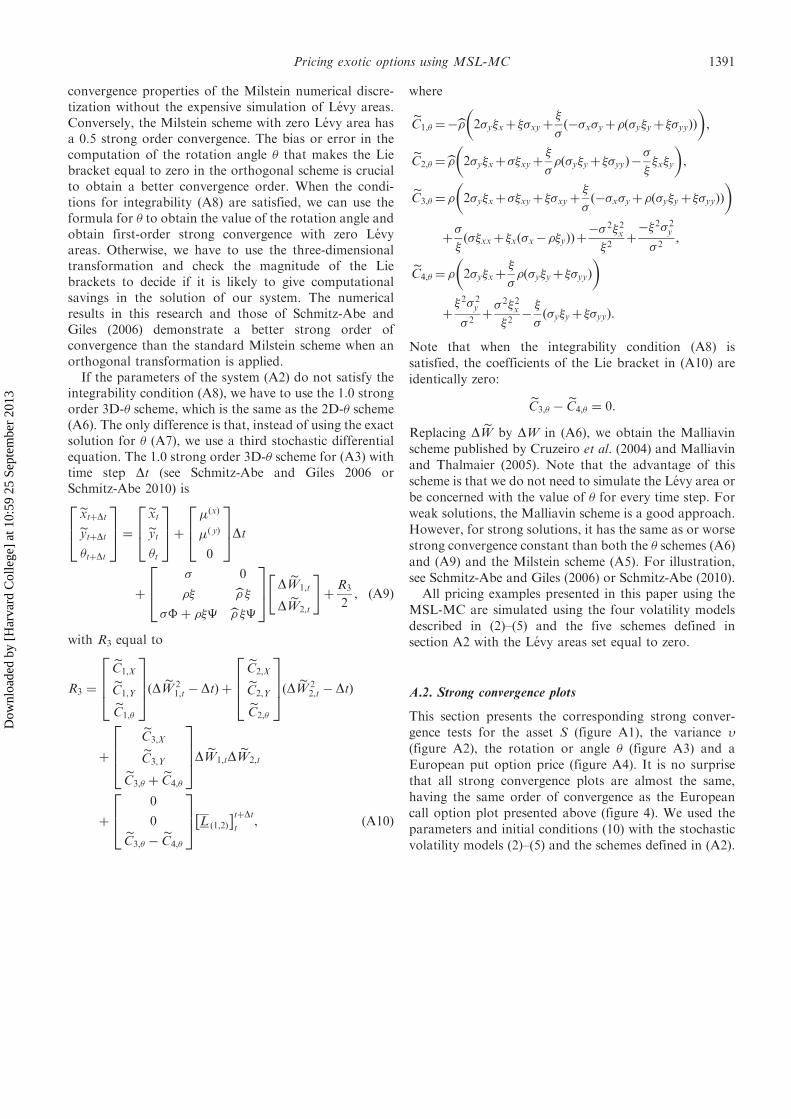
convergence properties of the Milstein numerical discre-tization without the expensive simulation of Levy areas.Conversely, the Milstein scheme with zero Levy area hasa 0.5 strong order convergence. The bias or error in thecomputation of the rotation angle � that makes the Liebracket equal to zero in the orthogonal scheme is crucialto obtain a better convergence order. When the condi-tions for integrability (A8) are satisfied, we can use theformula for � to obtain the value of the rotation angle andobtain first-order strong convergence with zero Levyareas. Otherwise, we have to use the three-dimensionaltransformation and check the magnitude of the Liebrackets to decide if it is likely to give computationalsavings in the solution of our system. The numericalresults in this research and those of Schmitz-Abe andGiles (2006) demonstrate a better strong order ofconvergence than the standard Milstein scheme when anorthogonal transformation is applied.

If the parameters of the system (A2) do not satisfy theintegrability condition (A8), we have to use the 1.0 strongorder 3D-� scheme, which is the same as the 2D-� scheme(A6). The only difference is that, instead of using the exactsolution for � (A7), we use a third stochastic differentialequation. The 1.0 strong order 3D-� scheme for (A3) withtime step Dt (see Schmitz-Abe and Giles 2006 orSchmitz-Abe 2010) is

extþDteytþDt�tþDt

264375 ¼ exteyt

�t

264375þ �ðxÞ

�ð yÞ

0

264375Dt

þ

� 0

�� b� ���þ ��� b� ��

264375 D eW1,t

D eW2,t

" #þR3

2, ðA9Þ

with R3 equal to

R3 ¼

eC1,XeC1,YeC1,�

26643775ðD eW 2

1,t � DtÞ þ

eC2,XeC2,YeC2,�

26643775ðD eW 2

2,t � DtÞ

þ

eC3,XeC3,YeC3,� þ eC4,�

26643775D eW1,tD eW2,t

þ

0

0eC3,� � eC4,�

264375 L 1,2ð Þ

tþDtt

, ðA10Þ

where

eC1,� ¼�b� 2�y�xþ ��xyþ�

�ð��x�yþ�ð�y�yþ ��yyÞÞ

� �,

eC2,� ¼b� 2�y�xþ��xyþ�

��ð�y�yþ ��yyÞ�

�

��x�y

� �,

eC3,� ¼ � 2�y�xþ��xyþ ��xyþ�

�ð��x�yþ�ð�y�yþ ��yyÞÞ

� �þ�

�ð��xxþ �xð�x���yÞÞþ

�� 2�2x�2þ��2� 2

y

� 2,

eC4,� ¼ � 2�y�xþ�

��ð�y�yþ ��yyÞ

� �þ�2� 2

y

� 2þ� 2�2x�2��

�ð�y�yþ ��yyÞ:

Note that when the integrability condition (A8) issatisfied, the coefficients of the Lie bracket in (A10) areidentically zero: eC3,� � eC4,� ¼ 0:

Replacing D eW by DW in (A6), we obtain the Malliavinscheme published by Cruzeiro et al. (2004) and Malliavinand Thalmaier (2005). Note that the advantage of thisscheme is that we do not need to simulate the Levy area orbe concerned with the value of � for every time step. Forweak solutions, the Malliavin scheme is a good approach.However, for strong solutions, it has the same as or worsestrong convergence constant than both the � schemes (A6)and (A9) and the Milstein scheme (A5). For illustration,see Schmitz-Abe and Giles (2006) or Schmitz-Abe (2010).

All pricing examples presented in this paper using theMSL-MC are simulated using the four volatility modelsdescribed in (2)–(5) and the five schemes defined insection A2 with the Levy areas set equal to zero.

A.2. Strong convergence plots

This section presents the corresponding strong conver-gence tests for the asset S (figure A1), the variance (figure A2), the rotation or angle � (figure A3) and aEuropean put option price (figure A4). It is no surprisethat all strong convergence plots are almost the same,having the same order of convergence as the Europeancall option plot presented above (figure 4). We used theparameters and initial conditions (10) with the stochasticvolatility models (2)–(5) and the schemes defined in (A2).

Pricing exotic options using MSL-MC 1391

Dow

nloa

ded

by [

Har

vard

Col

lege

] at

10:

59 2

5 Se

ptem

ber

2013

101

102

10−4

10−3

10−2

EX1; C4, T=10

101

102

10−4

10−3

10−2

EX2; C4, κ=10

101

102

10−5

10−4

10−3

EX3; C3, κ=0.2, β=0.2

101

102

10−3

10−2

EX4; C3, κ=0.2, β=3

101

102

10−4

10−3

10−2

EX5; C2, T=0.2, β=1

101

102

10−5

10−4

10−3

European Put

EX6; C2, T=0.2, β=3

101

102

10−2

NSteps

EX7; C4, ω=0.03 2

Euler schemeMilstein (L=0)Milstein sch.Malliavin sch.

2D θ scheme

3D θ sch (L=0)

3D θ scheme

Mea

n (|

erro

r|)

Mea

n (|

erro

r|)

Mea

n (|

erro

r|)

Mea

n (|

erro

r|)

Figure A4. Strong convergence tests for a European put optionusing (10).

101

102

10−4

10−3

10−2

10−1

EX1; C4, T=10

101

102

10−4

10−3

10−2

10−1

EX2; C4, κ=10

101

102

10−6

10−5

10−4

EX3; C3, κ=0.2, β=0.2

101

102

10−3

10−2

EX4; C3, κ=0.2, β=3

101

102

10−5

10−4

10−3

EX5; C2, T=0.2, β=1

101

102

10−4

10−3

Variance "v"

EX6; C2, T=0.2, β=3

101

102

10−3

NSteps

EX7; C4, ω=0.03 2

Euler schemeMilstein (L=0)Milstein sch.Malliavin sch.

2D θ scheme

3D θ sch (L=0)

3D θ scheme

Mea

n (|

erro

r|)

Mea

n (|

erro

r|)

Mea

n (|

erro

r|)

Mea

n (|

erro

r|)

Figure A2. Strong convergence tests for the variance � using (10).

101

102

10−3

10−2

10−1

Mea

n (|

erro

r|)

Mea

n (|

erro

r|)

Mea

n (|

erro

r|)

Mea

n (|

erro

r|)

EX1; C4, T=10

101

102

10−3

10−2

EX2; C4, κ=10

101

102

10−5

10−4

10−3

EX3; C3, κ=0.2, β=0.2

101

102

10−3

10−2

10−1

EX4; C3, κ=0.2, β=3

101

102

10−4

10−3

10−2

EX5; C2, T=0.2, β=1

101

102

10−4

10−3

Asset "S"

EX6; C2, T=0.2, β=3

101

102

10−2

NSteps

EX7; C4, ω=0.03 2

Euler schemeMilstein (L=0)Milstein sch.Malliavin sch.

2D θ scheme

3D θ sch (L=0)

3D θ scheme

Figure A1. Strong convergence tests for S using (10).

101

102

10−3

10−2

10−1

EX1; C4, T=10

101

102

10−3

10−2

10−1

EX2; C4, κ=10

101

102

10−5

10−4

10−3

EX3; C3, κ=0.2 , β=0.2

101

102

10−2

10−1

EX4; C3, κ=0.2, β=3

101

102

10−5

10−4

10−3

EX5; C2, T=0.2, β=1

101

102

10−4

10−3

10−2

"θ"

EX6; C2, T=0.2, β=3

101

102

10−1

100

NSteps

EX7; C4, ω=0.03 2

Euler schemeMilstein (L=0)Milstein sch.Malliavin sch.

2D θ scheme

3D θ sch (L=0)

3D θ scheme

Mea

n (|

erro

r|)

Mea

n (|

erro

r|)

Mea

n (|

erro

r|)

Mea

n (|

erro

r|)

Figure A3. Strong convergence tests for � using (10).

1392 K. Schmitz Abe

Dow

nloa

ded

by [

Har

vard

Col

lege

] at

10:

59 2

5 Se

ptem

ber

2013