First-Year Summer Project:

Pricing and Inventory Management under

Fluctuating Costs

Renyu Zhang

August 14, 2012

Contents

1 Industry Practice 2

1.1 Factors that Drive Price Fluctuation . . . . . . . . . . . . . . . . . . . . 2

1.2 Managing Price Fluctuation . . . . . . . . . . . . . . . . . . . . . . . . . 4

2 Literature Review 5

2.1 Production with Hedging and Speculation . . . . . . . . . . . . . . . . . 6

2.2 Optimal Inventory Policy under Price Uncertainty . . . . . . . . . . . . . 7

2.3 Inventory Management with Financial Instruments . . . . . . . . . . . . 11

2.4 Global Supply Chain Management . . . . . . . . . . . . . . . . . . . . . 16

3 Future Research Directions 19

Acknowledgements 20

1

2

1 Industry Practice

In the recent past, commodity prices have experienced not only dramatic rises but also

sharp falls. Such unpredictable price fluctuations prevail in today’s unstable global eco-

nomic climate, presenting great challenges for the firm’s pricing and inventory (procure-

ment and processing) decisions. In the manufacturing industry where the profit of a

firm highly depends on the prices of raw materials or items containing large amounts

of such materials, companies are forced to take the commodity risk management, which

deals with the price fluctuations of raw materials, seriously. According to a survey by

the Efficio Consulting, more than 55 percent of procurement executives said commodity

price instability was their single biggest challenge (Jenkinson, 2011). It is also estimated

that an approximate loss of half a billion Euros in 2010 due to higher raw material costs

(Sebastian and Maessen, 2010). In the global market, it is completely normal for firms to

have overseas sourcing opportunities. The uncertainty in exchange rate, labor cost and

tax rate will all contribute to a firm’s fluctuating input costs if he lies in the global supply

chain. For example, long-term growth in worldwide demand, coupled with a slowdown in

agricultural production growth, reduced global stockpiles of basic commodities like corn,

soybeans, wheat, and rice. Lower stocks, in turn, made it more likely that new sources

of demand, or disruptions to supply, precipitated sharply changing prices. See Schwartz

(2009) for reference in the fluctuating food commodity prices and Crenshaw etal. (2010)

for the random and rapidly increasing oil prices.

1.1 Factors that Drive Price Fluctuation

The up-and-downs of raw material prices are primarily driven by supply and demand

(Sebastian and Maessen, 2010). The Japan earthquake in 2010, for example, inevitably

raised quite a large spectrum of industry products. A change in government, legislative

bodies, other foreign policy makers, or military control can constrain oil production,

especially in countries like Iran, Iraq and Nigeria. The supply disruption will naturally

give rise to acute price increase. Other traditional factors like reserve level, free capacity

and current inventory all contribute significantly to the fluctuation of several storable

commodities like oil and natural gas.

Most economic analysts agree that the simple laws of supply and demand are work-

ing but speculation in the market has caused an increase in demand, and is the major

debate among economists and financial analysts (Crenshaw etal. 2010). Speculative and

investment-grade money entering the commodities market has attributed to the recent

2

3

price increase. People want to own contracts, and this has created additional demand.

In an effort to spread out the risk and take advantage of opportunities, investment funds,

retirement funds and insurances are investing in the commodity market, according to

Sebastian and Maessen, 2010. It is also emphasized that speculations only strength the

up and down trend. They do not set specific trend, but go wherever looks best.

The uncertain exchange and interest rates may also be a contributing factor of some

commodity price fluctuations. For example, since oils are priced using dollars, the varying

status of the US dollar is another cause of the fluctuating oil price. In 2007, low rates

and decreasing dollar value together lead to high oil prices (Crenshaw etal. 2010).

Last but not least, the trading market condition is also another complicated factor

that affect commodity prices (See Nationwide Insurance Company website http://www.

nationwide.com/rss/gas-prices-fluctuation.jsp, for example.). There are usually

three different markets that play a role in the price of commodities like gasoline.

• Contract market

Contracts among oil companies, dealers, refineries and independent dealers crucially

predetermine the price of a lot of commodities, say oil, gas, copper and several food

commodities.

• Spot market

The spot market can be used to fill the gaps in the contracts market by matching

companies with surplus commodities to those that need more. Of the three markets,

the spot market is the only one where actual commodities, say barrels of oil, are

traded. Best deals are also found there because buyers and sellers are not bound

by contracts.

• Futures market

Crude oil, for example, is traded on the New York Mercantile Exchange, although

contracts are rarely fulfilled. More than 5 billion barrels of oil were reportedly

traded on the futures market during a seven-year period, however, only 31,000

were actually delivered. The information on the status of the commodity market

motivates the fluctuation. In general, consumer gasoline prices will follow the trends

of the crude oil futures market.

3

4

1.2 Managing Price Fluctuation

To manage the risk of commodity price fluctuation, the firm makes several attempts,

say inventory management, contract optionality and passing cost increase to customers

to dampen the influence of such volatility. The fundamental idea is that the should

assess risks and opportunities from price volatility accurately and adapt its inventory

and pricing decisions accordingly.

Intuitively speaking, the firm should pass the cost uncertainty to customers. This

suggestion is correct but somewhat trivial. However, this is really an uneasy task. Cus-

tomers are hardly willing to bear the cost risk alone if they do not have any chance to

pass on the costs to his buyers. For some products, the value added to it is very high

and the firm will earn a high gross margin. For example, branded pharmaceuticals and

specialized electronics (e.g. IPAD) all fall into this category. The firm not only has

high freedom to price the product but also enjoys low dependence on the raw materials.

Hence, the firm’s pricing mainly depends on the demand (customer) side instead of the

supply side. Therefore, raw material price fluctuations will not have very big impact on

the firm’s pricing and inventory decisions, neither will it greatly affect its profit. For

other products, however, the margin is very low and the raw material costs contribute

to a large proportion of the the product. Products of this category include, for example,

modeled plastic and petrochemicals. In this case, the high competitive intensity is the

reason why costs increase cannot be converted into price change. The firm will suffer

greatly from raw material price fluctuations because the pricing freedom it has is very

limited.

In the face of rapid price fluctuation, the first thing a firm needs to do is to move

away from rigid pricing and procurement systems (Sebastian and Maessen, 2010). Annual

contracts, for example, may not be a suitable choice in the highly volatile current raw

material market. In this dynamic market and cost environment, shorter terms (quarterly

or monthly contracts) will enable the firms to better responsively and accurately assess

the price opportunities. The gap between contact prices and spot market prices also

decrease with quarterly or monthly contracts. Shortening the negotiation cycle can also

create more opportunities for the firm to better deal with raw material cost fluctuations.

It is also a good idea to add escalation clauses so that the firm can call for an adjustment

in the event of an increase or decrease in certain costs. See Kinlan and Roukema (2011),

for example. The escalation clause also helps firms to cover the costs resulting from

fluctuations.

Effectively managing the inventory may also help mitigate the risk of fluctuating input

4

5

costs. A better forecast of price and cost is thus essential. If the input cost is predicted

as up-sloping, the firm should adjust the inventory up. This is called investment buying

in the literature which is also widely used in pharmaceutical industry (Schwarz and

Zhao 2011). Reversely speaking, if the cost is forecasted downward sloping, the firm

should, instead, hold as little inventory as possible. The joint operational and financial

hedging is also a widespread approach to address the highly fluctuating costs. The firms

hardly put all their eggs in one basket so they usually outsource their inputs to multiple

suppliers. The multiple sourcing strategy not only reduces the supply disruption risk but

also enables the firm to dampen the procurement cost uncertainty. To better accomplish

this goal, the firm’d better unbundle the costs of his suppliers and decide how much of the

cost is driven by a particular commodity (Jenkinson, 2011 and Barosi and Busse, 2011).

Financial hedging, on the other hand, also serve as a powerful weapon against input price

fluctuations. Futures, swaps, options, and fixed-price agreements can all be employed for

a cost to help avoid significant unexpected price increases (Barosi and Busse, 2011).

Essentially, hedging raw materials or currencies on contract markets can be considered

as paying a price for certainty and the firm should also bear the risk of price drop.

As an end note, we point out an innovative idea proposed by Monsanto’s former CEO

R. J. Mahoney: when facing the rapid fluctuating prices, there are usually three choices:

(1) risk it; (2) take contingent actions like hedging and (3) avoid it. Mr. Mahoney

chose the third option. He was tired of having the wild swings in oil prices that decide

their profitability because the company was upgrading oil to petrochemicals and their

derivatives like plastics and fibers. As a consequence, he sold off some 8 billion dollars of

chemical businesses and bought into biology, where their brains would determine results

not the price of oil. Fortunately, it worked.

2 Literature Review

There is a large volume of literature that deals with the supply risk originating from

the fluctuating procurement price. In theoretic literature, the underlying driven force

of the price fluctuation is usually indebted to the dynamic imbalance between supply

and demand and the behavior of the inventory holders that buy low and sell high (i.e.

speculation). See Gustafson (1958), Deaton and Laroque (1992,1996), Chambers and

Bailey (1996), Williams and Wright (1991) and Borenstein etal. (1997) for details. The

rational expectation theory and how it influences the price movements dates back to Muth

(1961) and is also applied in the study of production-inventory systems (2010) whereas

5

6

the stochastic speculative price theory is comprehensively treated in Kaldor (1939) and

Samuelson (1970,1973). The interaction of inventory and price dynamics is also carefully

studied in the literature. See Pindyke (1994) or Geman (2005), for example. Based on

the notion of convenience yield, Gibson and Schwartz (1990), Schwartz (1997), Schwartz

and Smith (2000) and Casassus and Collin-Dufresne (2005) present some models that

depict the stochastic evolution of commodity prices.

2.1 Production with Hedging and Speculation

In production economics literature, there are a stream of papers that address the issue

of how a firm in the manufacturing industry should deal with price fluctuation, possibly

with hedging and speculation. Sandmo (1971) and Batra and Ullah (1974) examines

the behavior of a competitive firm being faced with input-hiring decisions under price

uncertainty. Let U(π) stands for the utility of the firm with profit π, where U ′(π) > 0

and U ′′(π) < 0. Assume that the cost function C(x) is strictly increasing. The firm’s

total profit is

π = px− C(x),

where p is the nonnegative random variable of the product price. The objective of the

firm is to maximize the expected utility

E{U(px− C(x))}.

Sandmo (1971) and Batra and Ullah (1974) show that the firm will underinvest and

underproduce with price uncertainty giving rise to a declination in the firm’s output while

the declination is increasing in the uncertainty of the price. This is intuitively correct

because as the price uncertainty grows, the firm will bear more risk. For a risk-averse

firm, it should produce less to reduce such additional risk.

Holthausen (1979) and Feder etal. (1980) demonstrate that using future contracts

can help the firm to hedge or even speculate against price uncertainty. Suppose the firm

sells the product either at stochastic price p or as forward contract at the certain price b.

The amount of output sold in the forward market is h. The objective function, defined

as the expected utility of profit,

E{U(π)} = E{U [p(x− h) + bh− c(x)]}.

The first order conditions with respect to x and h imply that the production quantity x

only depends on the price of the forward b, so the firm will not underproduce. Whether

6

7

the risk-averse firm should hedge its entire output (h = x) or hedge less than then entire

output (0 < h < x) or speculate (h > x and h < 0) depends on the comparison between

the forward price b and the expected stochastic price E{p}. In short, if b = E{p}, thefirm should hedge the entire production (h = x); if b > E{p}, the firm should speculate

by selling forward an amount greater than its output (h > x), expecting to purchase the

additional output in the future at a lower price in the open market; if b < E{p}, the firmshould either hedge part of its production (0 < h < x) or speculate by purchasing output

in the forward market (h < 0), expecting to sell the additional output at a greater price

in the forward market. In a healthy economy, the firm should pay for certainty (b < E{p}but b is not too small compared with E{p}) and the optimal policy is to hedge part of

the production with forward contract (0 < h < x). Otherwise, the firm may speculate

by selling more than it produces (h < 0 or h > x).

Models that address the issue of optimal hedging with multiple futures and/or multiple

periods are established in Anderson and Danthine (1981,1983), Meyer (1987) and Kamara

(1993). Lapan etal. (1991), Lence (1995) and Moschini and Lapan (1992), among others,

investigate the hedging behavior using options contracts.

2.2 Optimal Inventory Policy under Price Uncertainty

Quite a lot of papers make some attempt to understand the impact of stochastic spot

prices on the optimal inventory control policy over the decades. For example, Zheng

(1994) studies a single-item continuous-review inventory system with Poisson demand.

In addition to the standard cost structure of a fixed setup cost and a quasiconvex ex-

pected inventory holding and shortage cost, special opportunities for placing orders at

a discounted setup cost occur according to a Poisson process that is independent of the

demand process. Let the single item inventory system faces a Poisson demand process

of rate λ. Unsatisfied demand is assumed to be fully backlogged. The continuously re-

viewed system has constant replenishment lead time. The ordinary setup cost is K per

order whereas the discounted setup cost is k (k < K). The discount opportunity epochs

form a Poisson process, independent from the demand process, of rate µ. Therefore, the

decision epochs form a Poisson process of rate λ + µ. The objective is to figure out the

replenishment policy that minimizes the order (setup and unit) and operating (holding

and backorder) costs. order policy The optimal policy is shown to be of (s, c, S) type. i.e.

an order is placed to raise the inventory position to S either when the inventory position

drops to s or when the inventory position is below or at c (c ≥ s) when a discount op-

portunity occurs. The paper also develops an efficient algorithm for computing optimal

7

8

control parameters (s∗, c∗, S∗). Similar models are also discussed in Friend (1960), Moin-

zadeh (1997) and Feng and Sun (2001) where discount opportunities occur randomly and

Markovianly.

Kalymon (1971) studies a multi-period stochastic inventory model in which the pro-

curement price is driven by a Markovian process. In period i, xi refers to the inventory

before ordering, yi is the inventory after ordering, Di is the demand that depends on the

price of this period pi. The price process {pi} is assumed to be a non-stationary Markov

process. The period index i is labeled backwardly.

Ci(yi − xi|pi) , Kiδ(yi − xi) + pi(yi − xi)

is the ordering cost of period i, where Ki ≥ 0 is the setup cost, δ(z) = 1 for z > 0 and 0

for z = 0, and yi ≥ xi.

Li(yi|pi) , EDi{h(yi −Di)|pi}

denotes the expected holding and backorder costs where h(z) ≥ 0 and is a convex function

such that h(0) = 0, limz→±∞ h(z) = ∞. Let fi(x, p) be the minimum accumulative cost

of the firm in period i with inventory x and facing price p. The Bellman equation is

characterized as follows:

fi(x, p) = infy≥x

Ci(y − x|p) + Li(y|p) + αEpi−1,Di{fi−1(y −Di, pi−1)|p},

where α is the discount factor and f0(x, p) ≡ 0. Kalymon (1971) shows that the price-

dependent (s, S) is optimal, determines the bounds of the control bands s(p) and S(p)

and discusses computational approaches exploiting structure.

Using single unit decomposition approach, Berling and Martınez-de-Albeniz (2011)

makes some effort to characterize the optimal base-stock inventory policy when the pur-

chase price either follows a geometric Brownian motion or an OU process. Assume that

the firm needs a commodity as an input for production. The commodity bought in a spot

market with quoted price C(t) = ec(t). The log-price c(t) evolves in a one-factor model

with drift µ(c) and variance σ(c)2. i.e.

dc(t) = µ(c)dt+ σ(c)dWt,

where Wt is the standard (one dimensional) Brownian motion. For the geometric Brow-

nian motion, µ(c) = µ and σ(c) = σ while for the Ornstein-Uhlenbeck process, µ(c) =

−κ(c− c) and σ(c) = σ. The demand arrival process is a Poisson process of rate λ. The

single-echelon continuous-time review system has constant lead time L. The holding cost

8

9

is h per unit time whereas the backlog cost is b. The objective is, as usual, to mini-

mize the long run average cost. Based on the continuous-time-review counterpart of the

result in Kalymon (1970), the optimal inventory policy is an (s(c), S(c)) policy, where

s(c) = S(c)− 1 because the setup cost is zero.

Denote ti as the ordering time of the ith unit of ordering and we assume that the

placed order cannot be canceled. Let Ti be the arrival time of the corresponding demand

of the ith ordering and r be the discount factor, so the objective is to minimize

E{∫ +∞

t=0

[h+∞∑i=1

1ti+L≤t≤Ti+ b

+∞∑i=1

1Ti≤t≤ti+L + C(t)+∞∑i=1

δ(t− ti)]e−rtdt}

=+∞∑i=1

E{∫ +∞

t=0

[h1ti+L≤t≤Ti+ b1Ti≤t≤ti+L + C(t)δ(t− ti)]e

−rtdt, }

where 1· is the indicator function and δ(·) is the dirac function such that∫ +∞

z=−∞f(z)δ(t− z)dz = f(t).

Because the demand arrives as a Poisson process and the price process is also Markovian,

whether ti = t (ordering now) only depends on the current inventory k := i −D[0,t] and

log-price c(t). The remaining arrival for customer i only depends on k and follows an

Erlang distribution of rate λ and index k . i.e. Ti − t ∼ Ek. Therefore, the problem for

the ith ordering can be reformulated as

J(k, c(t)) = minτ≥t

E{∫ +∞

u=0

[h1τ−t−+L≤u≤Ek+ b1Ek≤u≤τ−t+L + ec(u)δ(u− τ + t)]e−rudu},

Where J(k, c(t)) is the cost-to-go function at time t with inventory k and log-price c(t). If

the firm chooses to order one unit when the inventory is k, the cost should be ec(t)+Π(k),

where Π(k) is the expected net present value of future holding and backorder costs when

the inventory is k. For a complete characterization of Π(k), please refer to Berling

and Martınez-de-Albeniz (2011). To get the Hamilton-Jacobi-Bellman equation that

J(k, c(t)) satisfies, we observe that if the current customer has already arrived, i.e. k ≤ 0,

J(k, c) = J(0, c) should satisfy the following HJB equation:

b− rJ(0, c) + µ(c)∂J

∂c(0, c) +

σ2(c)

2

∂2J

∂c2(k, c) = 0,

which follows directly from stochastic control theory. The boundary condition is also

intuitive J(0, c) → b/r indicating that when the price is really high, it would be optimal

to pay the backorder cost rather than ordering cost. If k ≥ 1, the HJB equation can be

9

10

written as

−(r + λ)J(k, c) + λJ(k − 1, c) + µ(c)∂J

∂c(k, c) +

σ2(c)

2

∂2J

∂c2(k, c) = 0.

The boundary condition can be summarized as

limc→+∞

J(k, c) =b

r(

λ

λ+ r)k.

Under certain technical conditions, for every k, there exists cLk and cHk such that, if

cLk ≤ c ≤ cHk , J(k, c) = ec + Π(k) and J(k, c) solves the HJB equations otherwise. The

computational approach is also proposed to the geometric Brownian motion model and

the OU process model to determine cLk , cHk and equivalently S(c) in Berling and Martınez-

de-Albeniz (2011).

There are also other papers that study the optimal inventory policy under price un-

certainty and we only discuss a few here. Zipkin (1989) studies an inventory system with

periodically varying demand and input price, which implies that the firm tends to order

up to a higher inventory level when the price is low. Scheller-Wolf and Tayur (1998) con-

siders a periodic-review inventory system with capacitated order quantity and fluctuating

cost which depends on the exchange rate. Gavirneni (2004) shows that the order-up-to

policy is optimal when the unit purchasing cost is fluctuating according to Markov chain

and the order-up-to level is decreasing unit cost under certain conditions. Chen and Song

(2001) derives structural policies for multi-echelon systems with Markov-modulated de-

mand. In Golabi (1985), the demand is deterministic and must be completely satisfied.

The paper determines how many periods of demand ahead the firm should satisfy when

the ordering price is random.

In recent years, a new line of research that combines the classical inventory theory and

commodity price theory mentioned above. See Haksoz and Seshadri (2007) for a review.

The approximate approach is developed in Berling and Rosling (2005) and Berling (2006)

whereas the periodic review models can be found in Goel and Gutierrez (2011a). Berling

and Rosling (2005) discusses how the financial risks and option valuation will influence

the (R,Q) inventory policy under optimality while Berling (2006) studies the valuation

of the inventory holding cost under the stochastic mean-reverting purchase price. In Goel

and Gutierrez (2011a), a model for the procurement of traded commodities is developed

and the optimal regulated band policy is proposed and algorithmically characterized. Yi

and Scheller-Wolf (2003) investigates the optimal dual sourcing policy with a regular

supplier and spot market.

10

11

2.3 Inventory Management with Financial Instruments

A great many of recent papers contribute to the application of financial instruments to

hedge against fluctuating price risks in the operations management setting. Gaur and

Seshadri (2005) contributes to the understanding of hedging inventory risk for a short life

cycle or seasonal item when its demand is correlated with the price of a financial asset.

Consider a single-period, single-item inventory model with stochastic demand, i.e., the

newsvendor model. Assume that the demand forecast for the item is perfectly correlated

with the price at time T of an underlying asset that is actively traded in the financial

markets.

Let p denote the selling price of the item, c the unit cost, s the salvage value, I

the stocking quantity, and D the demand. The firm purchases quantity I at time 0

and demand occurs at a future time T . Demand in excess of I is lost, and any excess

inventory is liquidated at the salvage price of s. Without hedging, the cash flow at time

0 is therefore

Π0U(I) = −cI,

and at time T is

ΠTU = pmin{D, I}+ s(I −D)+.

Suppose the demand is perfectly correlated with the price of the financial asset, ST :

D = a + bST . Under, risk neutral measure, S0 = e−rTEN{ST}. Under financial hedging

with this asset (the details and proposed in Gaur and Seshadri, 2005), the profit of the

firm is:

ΠH(I) = (p− s)bS0 + e−rT [(p− s)a+ sI]− (p− s)be−rTEN [ST − (I − a)/b]+ − cI.

We have that EN [ΠU(I)] = ΠH(I) and V ar(ΠH(I)) = 0, where ΠU(·) stands for the

total unhedged profit discounted to time 0. The paper also discusses the cases where

the demand is not perfectly correlated with asset price and risk-averse firm. See Gaur

and Seshadri (2005) for details. Caldentey and Haugh considers a similar problem in the

continuous time setting. They consider the problem of dynamically hedging the profits of

a firm when these profits are correlated with returns in the financial markets. In particu-

lar, The general problem of simultaneously optimizing over both the operating policy and

the hedging strategy of the firm is analyzed in this paper. Akella etal. (2002) and Wu

and Kleindorfer (2005) summarize the procurement and supplier risk management in B-

to-B e-business markets. Dong and Liu (2007) derives the equilibrium forward contracts

11

12

on non-storable commodities between two firms that have mean-variance preference and

negotiate their forward contracts through Nash bargaining.

The portfolio effects of option contracts and spot markets are analyzed in Fu etal.

(2010) and Martınez-de-Albeniz and Simchi-Levi (2005) the former of which proposed

an optimal procurement policy by the shortest monotone path algorithm and the latter

establishes the optimality of a modified base-stock policy. Fu etal. (2010) develops a

single period model that analyzes the value of portfolio procurement in a supply chain

where a buyer can either procure parts for future demand from n sellers using fixed price

contracts or from a spot market. The buyer of a single item faces random demand D

and random spot market price Ps in a single period. For contract type i, the reservation

price is ci whereas the execution price is hi. The buyer first purchases options from the

n contracts to ensure Qi units of supply before the realization of D and Ps. After D and

Ps are realized, the buyer decides how much, upto the quantity specified in the contract,

to exercise (xi) from each of the contracts signed with the suppliers and how much to

procure from the spot market to satisfy the realized demand. Without loss of generality,

assume that h1 < h2 < · · · < hn and c1 > c2 > · · · > cn. The portfolio procurement

problem can be formulated as

minQi≥0,i=1,2,...,n

{n∑

i=1

ciQi + ED,Ps [minxi,y

(n∑

i=1

hixi + Psy)]},

subject to xi ≤ Qi and xi ≥ 0 for i = 1, 2, · · · , n, y ≥ 0 and∑

i xi + y ≥ D. A

shortest-monotone path algorithm is provided in Fu etal. (2010) for the optimal portfolio

procurement strategy of this problem. Again, this paper addresses the issue of the trade

off between higher cost and uncertainty.

Wu and Chen (2010) further investigates the relation between commodity inventory

and short-term price variation and characterizes the rational expectations equilibrium

for an economy in which competitive production firms link a raw material market and

a finished goods market, with uncertain and price-sensitive supply and demand. The

individual firm controls production and two stages of inventory under uncertain input

and output prices and operating costs. Let kt = (k1t, k2t, · · · , knt)′ be the n exogenous

factors which follow the following stochastic differential equation

dkt = µ0(kt)dt+ σ0(kt)dwt,

where µ0(·) is an n-dimensional vector-valued function, σ0)(·) is an n×m matrix-valued

function and wt is an m−dimensional standard Brownian motion. Let pt = (p1t, p2t)′,

12

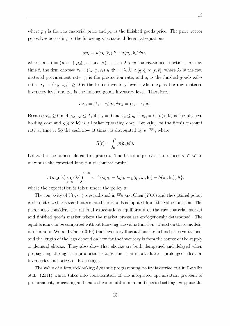
13

where p1t is the raw material price and p2t is the finished goods price. The price vector

pt evolves according to the following stochastic differential equations

dpt = µ(pt,kt)dt+ σ(pt,kt)dwt,

where µ(·, ·) = (µ1(·, ·), µ2(·, ·)) and σ(·, ·) is a 2 × m matrix-valued function. At any

time t, the firm chooses πt = (λt, qt, st) ∈ U = [λ, λ]× [q, q]× [s, s], where λt is the raw

material procurement rate, qt is the production rate, and st is the finished goods sales

rate. xt = (x1t, x2t)′ ≥ 0 is the firm’s inventory levels, where x1t is the raw material

inventory level and x2t is the finished goods inventory level. Therefore,

dx1t = (λt − qt)dt, dx2t = (qt − st)dt.

Because x1t ≥ 0 and x2t, qt ≤ λt if x1t = 0 and st ≤ qt if x2t = 0. h(x,k) is the physical

holding cost and g(q,x,k) is all other operating cost. Let ρ(kt) be the firm’s discount

rate at time t. So the cash flow at time t is discounted by e−R(t), where

R(t) =

∫ t

0

ρ(ku)du.

Let A be the admissible control process. The firm’s objective is to choose π ∈ A to

maximize the expected long-run discounted profit

V (x,p,k) supπ∈A

E{∫ +∞

0

e−Rt(stp2t − λtp1t − g(qt,xt,kt)− h(xt,kt))dt},

where the expectation is taken under the policy π.

The concavity of V (·, ·, ·) is established in Wu and Chen (2010) and the optimal policy

is characterized as several interrelated thresholds computed from the value function. The

paper also considers the rational expectations equilibrium of the raw material market

and finished goods market where the market prices are endogenously determined. The

equilibrium can be computed without knowing the value function. Based on these models,

it is found in Wu and Chen (2010) that inventory fluctuations lag behind price variations,

and the length of the lags depend on how far the inventory is from the source of the supply

or demand shocks. They also show that shocks are both dampened and delayed when

propagating through the production stages, and that shocks have a prolonged effect on

inventories and prices at both stages.

The value of a forward-looking dynamic programming policy is carried out in Devalka

etal. (2011) which takes into consideration of the integrated optimization problem of

procurement, processing and trade of commodities in a multi-period setting. Suppose the

13

14

time periods are indexed by n = 1, 2, · · · , N . The spot market price of the commodity

in period n is Sn. The deliver date of forward contract l ∈ {1, 2, · · · , L} is Nl (N1 <

N2 < · · · , NL). i.e. Nl − 1 is the last period that the firm can sell the output using

contract l. F ln denotes the period n forward price on contract l if n < Nl ≤ N . Let K

be the per-period procurement capacity and C be the processing capacity. The cost of

processing one unit of input commodity into output commodity is p. The firm incurs

per-period holding cost hI (hO) for input (output, respectively) commodity. Assume that

hO ≥ hI . Suppose the risk free discount factor is β. Under risk neutral measure, the

output forward prices for each contract must satisfy

En{F l+1m } = F l

n,

for n < Nl, ∀l, where En{·} is the conditional expectation operator on period n. For each

period n ≤ N − 1, the firm should decide the quantity of the input commodity to be

procured xn, the quantity to be processed mn and the quantity of the output commodity

to be committed for sale against forward contract l qln. Let Qn (en) be the total output

(input, respectively) inventory available at the beginning of period n.

Let l∗(n) be the optimal forward contract that the firm commits against in period n.

Therefore,

l∗(n) = argmaxl{βNl−nF ln − hO

Nl−n−1∑t=0

βt : l ≤ L,Nl > n}.

Let Vn(en, Qn) be the optimal profit-to-go in period n and the stochastic dynamic

program can be formulated in the following manner

Vn(en, Qn) = max0≤xn≤K,0≤mm≤min{C,en+xn},0≤q

l∗(n)n ≤Qn+mn

{[βNl∗(n)−nF l∗(n)n − hO

Nl−n−1∑t=0

βt]ql∗(n)n

− Snxn − pmn − hI(en + xn −mn)− hO[Qn +mn − ql∗(n)n ]

+ βEn[Vn+1(en + xn −mn, Qn +mn − ql∗(n)n )]},

(2.1)

where VN(eN , QN) = SNeN if QN ≥ 0 and −∞ if otherwise. Devalka etal. (2011)

shows that Vn(en, Qn) is linear in Qn and computes the marginal values of both input

commodity inventory and output commodity inventory in closed forms. It is found in

this paper that the optimal procurement and processing policies are governed by price-

dependent inventory thresholds.

Unlike most papers that consider the single location supply chain, Goel and Gutierrez

(2011b) analyzes a multiechelon distributional supply chain where the tradeoff between

14

15

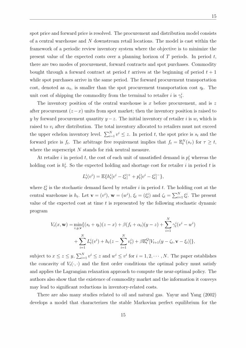
spot price and forward price is resolved. The procurement and distribution model consists

of a central warehouse and N downstream retail locations. The model is cast within the

framework of a periodic review inventory system where the objective is to minimize the

present value of the expected costs over a planning horizon of T periods. In period t,

there are two modes of procurement, forward contracts and spot purchases. Commodity

bought through a forward contract at period t arrives at the beginning of period t + 1

while spot purchases arrive in the same period. The forward procurement transportation

cost, denoted as αt, is smaller than the spot procurement transportation cost ηt. The

unit cost of shipping the commodity from the terminal to retailer i is γit.

The inventory position of the central warehouse is x before procurement, and is z

after procurement (z−x) units from spot market; then the inventory position is raised to

y by forward procurement quantity y− z. The initial inventory of retailer i is wi which is

raised to vi after distribution. The total inventory allocated to retailers must not exceed

the upper echelon inventory level.∑N

i=1 vi ≤ z. In period t, the spot price is st and the

forward price is ft. The arbitrage free requirement implies that ft = ENt (sτ ) for τ ≥ t,

where the superscript N stands for risk neutral measure.

At retailer i in period t, the cost of each unit of unsatisfied demand is pit whereas the

holding cost is hit. So the expected holding and shortage cost for retailer i in period t is

Lit(v

i) = E{hit[vi − ξit]+ + pit[v

i − ξit]−},

where ξit is the stochastic demand faced by retailer i in period t. The holding cost at the

central warehouse is ht. Let v = (vi), w = (wi), ξt = (ξit) and ζt =∑N

i=1 ξit. The present

value of the expected cost at time t is represented by the following stochastic dynamic

program

Vt(x,w) =minz,y,v

{(st + ηt)(z − x) + β(ft + αt)(y − z) +N∑i=1

γit(vi − wi)

+N∑i=1

Lit(v

i) + ht(z −N∑i=1

vit) + βEQt [Vt+1(y − ζt,v − ξt)]},

subject to x ≤ z ≤ y,∑N

i=1 vi ≤ z and wi ≤ vi for i = 1, 2, · · · , N . The paper establishes

the concavity of Vt(·, ·) and the first order conditions the optimal policy must satisfy

and applies the Lagrangian relaxation approach to compute the near-optimal policy. The

authors also show that the existence of commodity market and the information it conveys

may lead to significant reductions in inventory-related costs.

There are also many studies related to oil and natural gas. Yayur and Yang (2002)

develops a model that characterizes the stable Markovian perfect equilibrium for the

15

16

storable commodity market with a small number of capacitated firms. In Secomandi

(2010), a model is developed to understand the optimal commodity trading with a capac-

itated storage asset. When the commodity spot price evolves according to an exogenous

Markov process, this work shows that the optimal inventory-trading policy of a risk neu-

tral firm is characterized by two-stage and spot-price dependent basestock targets. The

inventory trading decisions are made at given equally spaced points in time belonging to

T . j ∈ J = {1, 2, · · · , J} denotes the jth decision made at time τj ∈ T . The length

of review period is T . An action is denoted as a: A positive action corresponds to a

purchase followed by an injection, a negative action to a withdraw followed by a sale, and

zero is the do-nothing action. Assume that the receipt/delivery leadtime is zero.

The storage asset features minimum and maximum inventory features x and x, so

the feasible set is X = [x, x]. C > 0 (C < 0) is the injection (withdraw, respectively)

capacity. The commodity spot price is assumed to be sj for j ∈ J . {sj}Jj=1 is Markovian

whereas s1 is degenerate. The trading action a depends on the realized spot price s. Let

the payoff of this decision be pj(a, s). αW ≤ 1 and αL are the commodity price adjustment

factors. LetcW and cL be the positive marginal withdrawal and injection costs. Therefore,

pj(a, s) = −(αW s− cW )a if a < 0, 0 if a = 0 and −(αLs + cI)a if a > 0. A unit holding

cost h is also charged at each time τj. The cash flows are discounted from time τj back

to time τj−1 using δj. The Bellman equations that the optimal value function Vj(x, s)

should satisfy is as follows:

Vj(x, s) = maxa

{pj(a, s)− hx+ δjEj[Vj+1(x+ a, sj+1)]},

where VJ(x, s) = maxa{−(αW s− cW )a− hx}. The paper shows that with a capacitated

commodity storage asset the qualification of low and high prices depends on the firm’s

own inventory ability. The optimal policy structure is also fully characterized by two

stage and spot price dependent base stock targets which can be easily computed.

Lai etal. (2011) develops a heuristic model for strategic valuation of the real option

to store liquefied natural gas that integrates models of LNG shipping, natural gas price

evolution, and inventory control and sale into the wholesale natural gas market.

2.4 Global Supply Chain Management

In the recent decade, global supply chain management emerges as a lively stream of

research. Interested readers are referred to Kouvelis (1999), Cohen and Huchzermeier

(1999) and Bouabatli and Toktay (2004) for literature reviews. Kogut and Kulatilaka

(1994) considers a firm with operating flexibility to shift production between two man-

16

17

ufacturing plants located in different countries. Consider a firm which is evaluating a

project to invest in two manufacturing plants-one in the U.S. and the other in Germany.

The plants are identical in their technological characteristics and differ only in the prices

(evaluated in dollars) of the local inputs. The product of the firm is priced in a world

market, say in U.S. dollars, and fluctuations of the Euro/$ exchange rate do not affect

the dollar market price. The input cost rates in the two countries are equated by the real

exchange rate

P$ = θPG,

where P$ is the input cost rate in the U.S., PG = PES is the dollar value of input cost

rate in Germany, PE is the input cost rate valued in Euro, S is the nominal exchange

rate and θ is the effective real exchange rate. To elucidate the impact of exchange rate

uncertainty, we model the evolution of θ as a discrete time stochastic process which tends

to revert towards its equilibrium θ. The discrete-time mean reverting stochastic process

for the real exchange rate can be written as

∆θt = λ(θ − θt)∆t+ σθt∆Zθ,

where ∆Zθ follows a normal distribution of mean 0 and variance ∆t. Suppose the min-

imum cost of producing one unit of output within time interval ∆t is ψ$ = ψ(P$). Due

to the identical technology, the unit dollar cost function of the plant in Germany must

be ψE = ψ(PEθ). By definition, ψ(·) is homogeneous of degree 1, so ψ(PE) = ψ(θP$) =

θψ(P$). When θ < 1, the firm has more incentive to produce in Germany, whereas when

θ < 1, the firm has more incentive to produce in U.S. Without loss of generality, the

costs of the U.S. plant is normalized to 1. So the dollar value of the German production

is ψG(θ) = ψ(θP$)/ψ(P$) = θ.

Suppose the firm knows with certainty the realized value of θt at the beginning of

each period. If switching plant location is costless, the optimal value in period t Ft(θt)

satisfies the following Bellman equation

Ft(θt) = min{1, ψG(θt)}+ ρEt{Ft+1(θt+1)},

where FT (θT ) = min{1, ψG(θT )} = min{1, θT} and ρ is the discount rate.

If, otherwise, the switching is costly, and the switching cost from location i to location

j is κij where 1 stands for U.S. and 2 stands for Germany. The Bellman equation then

becomes

Ft(θt, 1) = min{[1 + ρEtFt+1(θt+1, 1)], [κ12 + ψG(θt) + ρEt{Ft+1(θt+1, 2)}]}

17

18

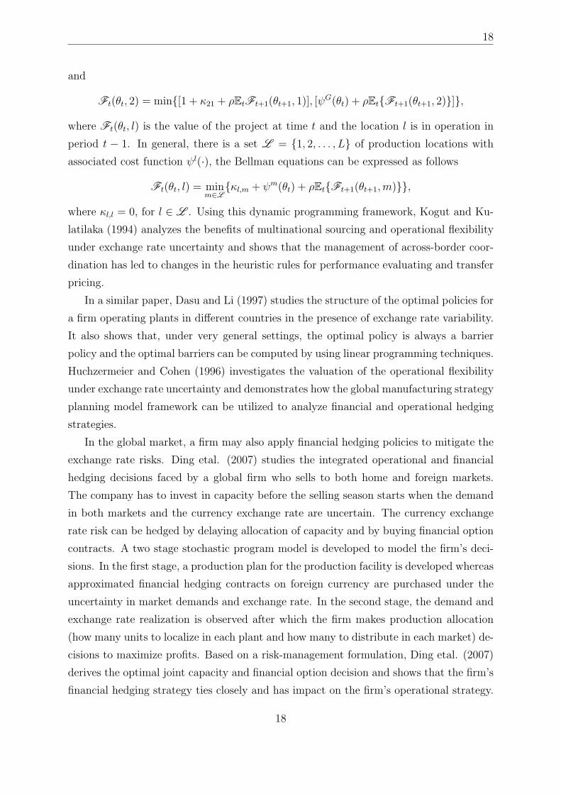
and

Ft(θt, 2) = min{[1 + κ21 + ρEtFt+1(θt+1, 1)], [ψG(θt) + ρEt{Ft+1(θt+1, 2)}]},

where Ft(θt, l) is the value of the project at time t and the location l is in operation in

period t − 1. In general, there is a set L = {1, 2, . . . , L} of production locations with

associated cost function ψl(·), the Bellman equations can be expressed as follows

Ft(θt, l) = minm∈L

{κl,m + ψm(θt) + ρEt{Ft+1(θt+1,m)}},

where κl,l = 0, for l ∈ L . Using this dynamic programming framework, Kogut and Ku-

latilaka (1994) analyzes the benefits of multinational sourcing and operational flexibility

under exchange rate uncertainty and shows that the management of across-border coor-

dination has led to changes in the heuristic rules for performance evaluating and transfer

pricing.

In a similar paper, Dasu and Li (1997) studies the structure of the optimal policies for

a firm operating plants in different countries in the presence of exchange rate variability.

It also shows that, under very general settings, the optimal policy is always a barrier

policy and the optimal barriers can be computed by using linear programming techniques.

Huchzermeier and Cohen (1996) investigates the valuation of the operational flexibility

under exchange rate uncertainty and demonstrates how the global manufacturing strategy

planning model framework can be utilized to analyze financial and operational hedging

strategies.

In the global market, a firm may also apply financial hedging policies to mitigate the

exchange rate risks. Ding etal. (2007) studies the integrated operational and financial

hedging decisions faced by a global firm who sells to both home and foreign markets.

The company has to invest in capacity before the selling season starts when the demand

in both markets and the currency exchange rate are uncertain. The currency exchange

rate risk can be hedged by delaying allocation of capacity and by buying financial option

contracts. A two stage stochastic program model is developed to model the firm’s deci-

sions. In the first stage, a production plan for the production facility is developed whereas

approximated financial hedging contracts on foreign currency are purchased under the

uncertainty in market demands and exchange rate. In the second stage, the demand and

exchange rate realization is observed after which the firm makes production allocation

(how many units to localize in each plant and how many to distribute in each market) de-

cisions to maximize profits. Based on a risk-management formulation, Ding etal. (2007)

derives the optimal joint capacity and financial option decision and shows that the firm’s

financial hedging strategy ties closely and has impact on the firm’s operational strategy.

18

19

3 Future Research Directions

Based on our analysis of the industry practice and literature, there are various directions

we think fruitful for future research.

We believe that the combined inventory and pricing management in the face of pro-

curement price uncertainty is a promising direction of future direction. Intuitively speak-

ing, pricing control adjusts the demand side of the system and has the following two

effects: (1) it can serve as a lever to balance the demand to the most profitable level in

accordance with the fluctuating procurement price; (2) the firm can apply price adjust-

ment to pass the procurement cost risk to its customers. On the other hand, inventory

management controls the supply side of the story. The firm should deal with both the

trade off between understock and overstock as well as the risk of fluctuating prices. As is

discussed in the first part of this paper, these two controls are jointly employed by firms

in practice. However, very few papers in OM literature make some effort to analyze the

optimal joint inventory and pricing policy while there are quite numerous papers that

merely discuss the optimal inventory policy. Wu and Chen (2010) is maybe the only one

that touches this issue, but this paper only establishes the rational expectation equilib-

rium but not the optimal inventory and pricing decision. To rigorously understand how

the two sources of uncertainty (price and demand) correlate with the control methods of

both supply (procurement) and demand (pricing) side is both interesting and challenging.

There are some fundamental questions that need to be addressed, among which are, for

example, the structure of the optimal policy and how the optimal policy should change

with the procurement price. Additionally, the analysis of the firms with different degrees

of pricing freedom is also interesting and promising. The optimal pricing and inventory

policy of the firm with high pricing freedom and large gross margin must differ signifi-

cantly from the one with limited market power and small margin. Very little literature

tries to understand the value of pricing freedom and the optimal policy of low pricing

freedom and low margin firm, which we believe is very important in practice.

Most papers in the literature that analyze the system facing price fluctuation only

consists of a single echelon firm. It is a promising direction of future research to take into

account the multi-echelon supply chain, where different stages of the system may compete

or cooperate. Both the system-wise optimal policy for the multi-echelon supply chain and

the equilibrium of a competitive setting are worth investigating. The information sharing

and collaborative forecasting issue in the two-echelon supply chain is also very attractive.

Generally speaking, the supplier will have a more precise forecast of price uncertainty

whereas the retailer will be better aware of the trend of customer’s demand. As a result,

19

20

both players can potentially gain more profits through wise information sharing and

collaborative forecasting strategies.

Some practitioners also suggest that the financial constraint a firm has also highly

determines the optimal strategy of the firm. That is to say the amount of loan banks

can lend will have a great impact on the optimal policy. This has yet been studied

in the literature, either. It is an interesting, also practical, problem to analyze the

optimal pricing and inventory policy when the inventory procurement is constrained by

its financial condition. Joint operational and financial hedging policy under financial

constraint is also not studied in the literature. However, it seems to us that this is also

a common approach in practice so it deserves the attention of academia.

As is suggested by Mr. Mohoney (see the first section of this paper), the firm usually

has three approaches in the face of rapidly increasing and fluctuating prices: (1) do

nothing and take the risk straightforwardly; (2) take contingent actions to hedge the

risk; and (3) avoid the risk by, for example, looking for an alternative supplier and

even changing the business it runs. This idea also relates to the degree of freedom and

flexibility the firm has. The more able the firm is to change its business, the higher degree

of flexibility it enjoys. The basic question in this line of research is that will the benefit

of avoiding fluctuating price risk over weighs the cost of changing a business. It is also

interesting and relevant to point out an effective way to evaluate this change. All these

are left to future research.

Acknowledgements

We thank R. J. Mohoney’s insightful comments as well as his thought-provoking sharing

of his executive experience on dealing with rapidly increasing and fluctuating prices.

References

[1] Ahn, H., M. Gumus, P. Kaminsky. 2007. Pricing and manufacturing decisions when

demand is a function of prices in multiple periods. Oper. Res. 55(6) 1039-1057.

[2] Akella, R., V. Araman, J. Kleinknecht. 2002. B2B markets: Procurement and sup-

plier risk management in e-business. J. Geunes, P. M. Pardalos, H. E. Romeijin, eds.

Supply Chain Management: Models, Applications and Research Directions. Kluwer

Academic, Dordrecht, The Netherlands, 33-68.

20

21

[3] Anderson, R. W., J. P. Dathine. 1981. Cross Hedging. J. Political Econom. 86(6)

1182-1196.

[4] Anderson, R. W., J. P. Dathine. 1983. The time pattern of hedging and the volatity

of future prices. Rev. Econom. Stu. 50(2) 249-266.

[5] Azoury, K. S. 1985. Bayes solution to dynamic inventory models under unknown

demand distribution. Management Sci. 31(9) 1150-1160.

[6] Barosi, F, P. Busse. 2011. Six stepts to managing raw material price volatility.

Alix Partners, December Issue. http://www.alixpartners.com/en/WhatWeThink/

HeavyEquipment/SixStepstoManagingRawMaterialPriceVolatilit.aspx

[7] Batra, R. N., A. Ullah. 1974. Competitive firm and the theory of input demand

under price uncertainty. J. Political Econom. 82(3) 537-548.

[8] Berling, P. 2008. The capital cost of holding inventory with stochastically mean-

reverting purchase price. Eur. J. Oper. Res. 186(2) 620-636.

[9] Berling, P., V. Martınez-de-Albeniz. Optimal inventory policies when purchase price

and demand are stochastic. Oper. Res. 59(1) 109-124.

[10] Berling, P., K. Rosling. 2005. The effects of financial risks on inventory policy. Man-

agement Sci. 51(12) 1804-1815.

[11] Borenstein, S., A. C. Cameron, R. Gilbert. 1997. Do gasoline prices respond asym-

metrically to crude oil price changes? Quart. J. Econom. 112(1) 305-339.

[12] Boyabalti, O., L. B. Toktay. 2004. Operational hedging: A review with discussion.

Working paper, INSEAD, France.

[13] Casassus, J., P. Collin-Dufresne. 2005. Stochastic convenience yield implied from

commodity futures and interest rates. J. Finance 60(5) 2283-2331.

[14] Chambers, M. J., R. E. Bailey. 1996. A theory of commodity price fluctuations. Rev.

Econom. Stud. 104(5) 2283-2331.

[15] Chan, L. M. A., Z.-J. M. Shen, D. Simchi-Levi, J. L. Swann. 2004. Coordination of

pricing and inventory decisions: A survey and classification. D. Simchi-Levi, S. D.

Wu, Z.-J. M. Shen, eds. Handbook of Quantitative Supply Chain Analysis: Modeling

in the E-Business Era. Springer Science + Business Media, New York, N.Y., 335-392.

21

22

[16] Crenshaw, L., B. Maniam, G. Subramaniam. 2010. Fluctuations in the price of oils

in the U.S.: Cause and effect. Rev. Bus. Res. 10(2) 2010.

[17] Ding, Q., L. Dong, P. Kouvelis. 2007. On the integration of production and financial

hedging decisions in global markets. Oper. Res. 55(3) 470-489.

[18] Chen, F., J. Song. 2001. Optimal policies for multiechelon inventory problems with

Markov-modulated demand. Oper. Res. 49(2) 226-234.

[19] Cohen, M. A., A. Huchzermeier. 1999. Global supply chain management: A survey

of research and applications. Chapter 20 of S. Tayur, R. Ganeshan, M. J. Maga-

zine (eds.), Quantitative Models for Supply Chain Mabagement, Kluwer Academic

Publishers, Netherland.

[20] Dasu, S., L. Li. 1997. Optimal operating policy in the presence of exchange rate

variability. Management Sci. 43(5) 705-722.

[21] Deaton, A., G. Laroque. 1992. On the behavior of commodity prices. Rev. Econom.

Stud. 59(1) 1-23.

[22] Deaton, A., G. Laroque. 1996. Competitive storage and commodity price dynamics.

J. Political Econom. 104(5) 896-923.

[23] Devalkar, S. K., R. Anupindi, A. Sinha. 2011. Integrated optimization of procure-

ment, processing, and trade of commodities. Oper. Res. 59(6) 1369-1381.

[24] Fabian, T., J. L. Fisher, M. W. Sasieni, A. Yardeni. Purchasing raw materials on a

fluctuating market. Oper. Res. 7(1) 107-122.

[25] Feder, G., R. E. Just, A. Schmitz. 1980. Futures markets and the theory of the firm

under price uncertainty. Quart. J. Econom. 94(2) 317-328.

[26] Feng, Y., J. Sun. 2001. Computing the optimal replenishment policy for inventory

systems with random discount opportunities. Oper. Res. 49(5) 790-795.

[27] Friend, J. K. 1960. Stock control with random opportunities for replenishment. Oper.

Res. Quart. 11 130-136.

[28] Fu, Q., C. Y. Lee, C. P. Teo. 2010. Procurement management using option contracts:

Random spot price and the portfolio effect. IIE Trans. 42(11) 793-811.

22

23

[29] Gaur, V., S. Seshadri. 2005. Hedging inventory risk through market instruments.

Mannufacturing Service Oper. Management 7(2) 103-120.

[30] Gavirneni, S. 2004. Periodic review inventory control with fluctuating purchasing

costs. Oper. Res. Lett. 32(4) 374-379.

[31] Geman, H., V. N. Nguyen. 2005. Soybean inventory and forward curve dynamics.

Management Sci. 51(7) 1076-1091.

[32] Gibson, R., E. S. Schwartz. 1990. Stochastic convenience yield and the pricing of oil

contigent claims. J. Finance 45(3) 959-976.

[33] Goel, A., G. J. Gutierrez. 2011a. Integrating commodity markets in the optimal

procurement policies of a stochastic inventory system. Working paper. University of

Texas at Austin.

[34] Goel, A., G. J. Gutierrez. 2011b. Multiechelon procurement and distribution policies

for traded commodities. Management Sci. 57(12) 2228-2244.

[35] Golabi, K. 1985. Optimal inventory policies when ordering prices are random. Oper.

Res. 33(3) 575-588.

[36] Gustafson, R. L. 1958. Carryover levels for grains: A method for determining

amounts that are optimal under specified conditions. United States Department of

Agriculture. 1-92.

[37] Haksoz, C., S. Seshadri. 2007. Supply chain operations in the presence of a spot

market: A review with discussion. J. Oper. Res. Soc. 58(11) 1412-1429.

[38] Holthausen, D. M. 1979. Hedging and the competitive firm under price uncertainty.

Amer. Econom. Rev. 69(5) 989-995.

[39] Huchzermeier, A., M. A. Cohen. 1996. Valuing operational flexibility under exchange

rate risk. Oper. Res. 44(1) 100-113.

[40] Jenkinson, J. 2011. Procurement in action, the efficio grassroots procurement

survey 2011. Efficio Consulting. http://www.efficioconsulting.com/ uploads/

documents/white-papers/procurement-in-action.pdf.

[41] Kalymon, B. 1971. Stochastic prices in a single-item inventory purchasing model.

Oper. Res. 19(6) 1434-1458.

23

24

[42] Kaldor, N. 1939. Speculation and economic stability. Rev. Econom. Stud. 7(1) 1-27.

[43] Kalymon, B. A. 1971. Stochastic prices in a single-item inventory purchasing model.

Oper. Res. 19(6) 1434-1458.

[44] Kamara, A. 1993. Production flexibility, stoochastic seperation, hedging, and futures

prices. Rev. Financial Stu. 6(4) 935-957.

[45] Kinlan, D., D. Roukema. 2011. When is an escalation clause necessary? Dealing

with price fluctuations in dredging contracts. Terra et Aqua 125 (December Issue)

3-9.

[46] Kogut, B., N. Kulatilaka. 1994. Operating flexibility, global manufacturing, and the

option value of a multinational network. Management Sci. 40(1) 123-139.

[47] Kouvelis, P. 1999. Global sourcing strategies under exchange rate uncertainty. Chap-

ter 20 of S. Tayur, R. Ganeshan, M. J. Magazine (eds.), Quantitative Models for

Supply Chain Mabagement, Kluwer Academic Publishers, Netherland.

[48] Lapan, H., G. Moschini, D. Hanson. 1991. Production, hedging and speculative

decisions with options and futures markets. Amer. J. Agri. Econom. 73 (1) 66-74.

[49] Lence, S. H. 1995. The economic value of minimum-variance hedges. Amer. J. Agri.

Econom. 77 (2) 353-364.

[50] Lai, G., M. X. Wang, S. Kekre, A. Scheller-Wolf, N. Secomandi. 2011. VAluation of

storage at a liquefied natural gas terminal. Oper. Res. 59(3) 602-616.

[51] Meyer, J. 1987. Two-moment decision models and expected utility maximization.

Amer. Econnom. Rev. 77(3) 421-430.

[52] Moinzadeh, K. 1997. Replenishment and stocking policies for inventory systems with

random deal offerings. Management Sci. 43(3) 334-342.

[53] Moschini, G., H. Lapan. 1992. Hedging price risk with options and futures for the

competitive firm with productin flexibility.

[54] Muth, J. F. 1961. Rational expectation and the theory of price movements. Econo-

metrica 29(3) 315-335.

[55] Pindyke, R. S. 1994. Inventories and the short-run dynamics of commodity prices.

RAND J. Econom. 25(1) 141-159.

24

25

[56] Samuelson, P. A. 1970. Stochastic speculative price. Proc. National Aca. Sci. 68(2)

335-337.

[57] Samuelson, P. A. 1973. Mathematics of speculative price. SIAM Rev. 15(1) 1-42.

[58] Sandmo, A. 1971. On the theory of the competitive firm under price uncertainty.

Amer. Econom. Rev. 61(1) 65-73.

[59] Schwartz, D. 2009. Fluctuating food commodity prices: A complex issue with no

easy answers. Oregon Wheat, Februrary issue, 8-11.

[60] Schwartz, E. S. 1997. The stochastic behavior of commodity prices: Implications for

valuation and hedging. J. Finance 52(3) 923-973.

[61] Schwartz, E. S., J. E. Smith. 2000. Short-term variations and long-term dynamics in

commodity prices. Management Sci. 56(3) 449-467.

[62] Schwarz, L., H. Zhao. 2011. The unexpected impact of information sharing on US

pharmaceutical supply chains. Interface 41(4) 354-364.

[63] Secomandi, N. 2010b. Optimal commodity trading with a capacitated storage asset.

Management Sci. 56(3) 449-467.

[64] Williams, J., B. Wright. 1991. Storage and Commodity Markets. Cambridge Univer-

sity Press, Cambridge, UK.

[65] Wu, D. J., P. R. Kleindorfer. 2005. Competitive options, supply contracting and

electronic markets. Management Sci. 51(3) 452-466.

[66] Wu, O. Q., H. Chen. 2010. Optimal control and equilibrium behavior of production-

inventory systems. Management Sci. 56(8) 1362-1379.

[67] Zheng, Y. S. 1994. Optimal control policy for stochastic inventory system with

Markovian discount opportunities. Oper. Res. 42(4) 721-738.

[68] Zipkin, P. H. 1989. Critical number policies for inventory models with periodic data.

Management Sci. 35(1) 71-80.

25