Munich Personal RePEc Archive

Price Dependence between Different Beef

Cuts and Quality Grades: A Copula

Approach at the Retail Level for the U.S.

Beef Industry

Papagiotou, Dimitrios and Stavrakoudis, Athanassios

University of Ioannina

17 March 2015

Online at https://mpra.ub.uni-muenchen.de/65451/

MPRA Paper No. 65451, posted 08 Jul 2015 05:38 UTC

Price Dependence between Different Beef Cuts and

Quality Grades: A Copula Approach at the Retail Level

for the U.S. Beef Industry

Dimitrios Panagiotou and Athanassios Stavrakoudis

Abstract

The objective of this study is to assess the degree and the structure of price dependence

between different cuts of the beef industry in the USA. This is pursued using the statistical

tool of copulas. To this end, it utilizes retail monthly data of beef cuts, within and between

the quality grades of Choice and Select, over the period 2000–2014. For the Choice quality

grade, there was evidence of asymmetric price co-movements between all six pairs of beef

cuts under consideration. No evidence of asymmetric price co-movements was found between

the three pairs of beef cuts for the Select quality grade. For the pairs of beef cuts formed

between the Choice and Select quality grades, the empirical results point to the existence of

price asymmetry only for the case of the chuck roast cut.

JEL codes: Q11, C13, L66

1

1 Introduction

Overwhelming evidence suggests that consumers perceive beef as a differentiated product. Phys-

ical intrinsic qualities like color, shape, appearance, tenderness, juiciness, flavor as well as its

nutritional properties (fatty acid composition) appear to influence consumers’ decisions when pur-

chasing beef. Data from Leick, Behrends, Schmidt, and Schilling (2012), indicate that consumers

may select cuts from the beef carcass that display certain quality attributes, even if there is a con-

siderable price difference.

Despite this fact, most of the studies on price dependence and asymmetric price response in

the U.S. beef industry have been carried out considering aggregate commodity prices. The quan-

titative tools utilized range from simple correlation analysis and regression models to recently

developed econometric approaches such as the linear error correction model (ECM), the asym-

metric non-linear ECM, the threshold vector ECM, the smooth transition cointegration model, the

Markov-switching ECM, and the copulas. Goodwin and Holt (1999), estimate a full vector error

correction model (VECM) of beef price relationships at the farm, wholesale and retail levels. The

authors found evidence of asymmetric price adjustment towards the equilibrium. Pozo, Schroeder,

and Bachmeier (2013), with the use of a threshold asymmetric error-correction model (TAECM),

find no evidence of asymmetric price transmissions (APT) in the response of retail beef prices to

changes in upstream prices. Emmanouilides and Fousekis (2014) assess the degree and the struc-

ture of price dependence along the U.S. beef supply chain utilizing the statistical tool of copulas.

Their empirical findings point to the existence of price transmission asymmetry, which is more

important for the pair wholesale–retail.

The USDA (United States Department of Agriculture (2014)) certifies and awards grades based

on different attributes of the beef carcass. In terms of quality, USDA awards three grades. USDA

Prime is the superior grade with amazing tenderness, juiciness, flavor and fine texture. It has the

highest degree of fat marbling and is derived from the younger beef. Prime is generally featured

at the most exclusive upscale steakhouse restaurants. USDA Choice is the second highest graded

beef. It has less fat marbling than Prime. Choice is a quality steak particularly if it is a cut that

is derived from the loin and rib areas of the beef such as a tenderloin filet or rib steak. Generally

2

USDA Choice will be less tender, juicy and flavorful with a slightly more coarse texture versus

Prime. USDA Select is generally the lowest grade of steak available at a supermarket or restaurant.

It is tougher, less juicy and less flavorful since it is leaner than Prime and Choice with very little

marbling. The texture of Select is generally more coarse1. In general, Prime (higher quality grade)

receives a higher price than Choice (lower quality grade), and Choice receives a higher price than

Select (lowest quality grade), both at retail and wholesale levels. Currently, about 3% of carcasses

grade as Prime, and 57% as Choice2.

Quality grades do not constitute the only beef attribute to determine consumers’ willingness

to pay. Consumers’ selections of ribeye, top loin, and sirloin steaks are impacted more by their

perception of thickness, marbling, and color than by price Leick et al. (2012). Different beef cuts

exhibit different prices. In general, cuts like ribs, loin, and sirloin are usually priced higher than

round or briskets, and cuts from the middle part of the animal are priced higher than cuts from the

ends of the carcass.

Against this background, the objective of this paper is to investigate if the existence of prod-

uct differentiation could be a source of asymmetric price comovements within certain beef quality

grades and beef cuts. Preference for specific quality attributes and cuts implies that consumers

have different marginal willingness to pay for these "different" beef products. Consequently, their

response might be different when prices change. At the same time, retailers can price discriminate

based on the different attributes of the commodity. This means that sellers might adopt differ-

ent pricing strategies, depending on the quality grade and cut, when market conditions change.

Conclusively, estimating price dependence while considering beef as a non-differentiated product,

would ignore differential responses. Empirical results may not capture the actual pricing behavior.

In our study, we estimate empirically price dependence between beef products differentiated by

quality and by cuts, at the retail level, with the use of the statistical tool of copulas. Copulas offer

an alternative way to analyze price co-movements, particularly during extreme market events. A

1For more details of exactly how a beef certifier measures marbling, maturity of the beef, the color of beef and its

texture to determine an accurate USDA Grade, we can go to the United States Standards for Grades of Carcass Beef

established by the United States Department of Agriculture – Agricultural Marketing Service (1997)2Wholesale cutout beef data available from USDA-Agricultural Marketing Service(AMS)

3

significant advantage of copulas is that they allow the joint behavior of random processes to be

modeled independently of the marginal distributions, providing this way considerable flexibility

in empirical research (Patton (2012)). Thus, copulas are a valuable tool for modeling the joint

behavior of random variables during extreme market events making it possible to assess whether

prices move with the same intensity during market upswings and downswings.

There are a few empirical studies, in agricultural economics, which have investigated mar-

ket dependence using copulas. Emmanouilides, Fousekis, and Grigoriadis (2013), assessed price

dependence in the olive oil market of the Mediterranean (Greece, Spain, and Italy). Reboredo

(2012) examined co-movement between international food (corn, soya beans and wheat) and oil

prices. Qiu and Goodwin (2012), estimated APT in the hog supply chain (case of vertical price

dependence).

To the best of our knowledge, there has been no published work which has examined price

co-movements between different cuts and quality grades of beef with the use of copulas.

The present work is structured as follows: Section 2 contains the theoretical framework. Sec-

tion 3 presents the data, the empirical models and the results. Section 4 offers conclusions.

2 Theoretical framework

2.1 Copulas and dependence measurement

Copula theory dates back to Sklar (1959), but only recently copula models have realized widespread

application in empirical models of joint probability distributions, see Nelsen (2007). Sklar proved

that a joint distribution can be factored into the marginals and a dependence function, which he

called "copula". Thus, he created a new class of functions (copulas) that tie together two marginal

probability functions that may be related to one another. Sklar showed that if G is a bivariate dis-

tribution function with margins G1(x) and G2(y), where (X,Y) are random processes, then there

4

exists a copula function C:[0,1]2 to [0,1] such that for every (x,y) ∈ R2 we have3

G(x,y) =C(G1(x),G2(y)) (1)

Given that the marginal distributions are continuous, C, G1(x), and G2(y) are uniquely deter-

mined by G(x,y). Conversely, for any pair (G1,G2) and for any copula C, the function G, written

in equation (1), defines a joint cdf for (X ,Y ) with margins G1 and G2. The copula can be obtained

from equation (1) in the following way:

C(u1,u2) = G(G−11 (u1),G

−12 (u2)) (2)

where G−1i , for i=(1,2), represent the marginal quantile functions, and ui represent quantiles on

U [0,1]. The joint pdf associated with the C copula function is obtained as:

c(u1,u2) =∂C2

∂u1∂u2=

g(G−11 (u1),G

−12 (u2))

g1(G−11 (u1))g2(G

−12 (u2))

=g(x,y)

g1(x)g2(y)(3)

where g is the joint pdf associated with G, and g1 and g2 are the marginals pdfs of X and Y

respectively. From equation (3) it follows

g(x,y) = c(G1(x),G2(y))g1(x)g2(y) (4)

From the equation above we can observe that the joint pdf contains information on the marginal

behavior of each random variable as well as on the dependence betwen them. The fact that the

marginal distributions become uniform means that the influences of the original marginal distri-

butions have been removed from the data. The only remaining feature is the way the transformed

random processes are paired, and the dependence between them is captured by the copula function,

which describes the way this "coupling" is done. It is evident from equation (4) that the copula

function fully describes the dependence of the random variables by capturing the information miss-

ing from the marginal distributions to complete the joint distribution, see Meucci (2011).

3For simplicity we consider the bivariate case. The analysis, however, can be extended to a m-variate case with

m>2.

5

Copulas are used to describe dependence (linear and non-linear) between random variables,

allowing the joint behavior of random processes to be modeled independently of the marginal

distributions. At the same time copulas link joint distribution functions to their one-dimensional

margins.

A rank based test of functional dependence is Kendall′s tau. It provides information on co-

movement across the entire joint distribution function, both at the center and at the tails of it. It is

calculated from the number of concordant and discondordant pairs of observations in the following

way:

τN =PN −QN(

N2

) =4PN

N(N −1)−1, (5)

where N represents the number of observations, and PN and QN denote the number of concor-

dant and discondordant pairs, respectively.4 Kendall’s tau captures co-movement across the entire

joint distribution function (center and tails).

Often though, information concerning dependence at the tails (at the lowest and the high-

est ranks) is extremely useful for economists, managers and policy makers. Tail (extreme) co-

movement is measured by the upper, λU , and the lower, λL, dependence coefficients defined as

λU = limu↑1

prob(U1 > u|U2 > u) = limu→1

1−2u+C(u,u)

1−u∈ [0,1], (6)

λL = limu↓0

prob(U1 < u|U2 < u) = limu→0

C(u,u)

u∈ [0,1], (7)

where λU measures the probability that X is above a high quantile given that Y is also above

that high quantile, while λL measures the probability that X is below a low quantile given that Y

is also below that low quantile. In order to have upper or lower tail dependence, λU or λL need

to be positive. Otherwise, there is upper or lower tail independence. Hence, the two measures of

tail dependence provide information about the likelihood for the two random variables to boom

4Two pairs (x j,y j), (xk,yk), j,k = 1,2, . . . ,N, are defined as concordant (discocordant) when (x j–xk),(y j–yk) > 0

(< 0).

6

and to crash together. It is worth noticing that since the tail coefficients are expressed via copulas

in equations (6) and (7) , certain properties of copulas apply to λU and λL (e.g. invariance to

monotonically increasing transformations of the variables).

Using copulas to describe dependence between random variables is very advantageous for the

researcher. First of all, copulas can model co-movement between these random processes indepen-

dently of the marginal distributions. Secondly, copulas allow for more flexible functional forms

of dependence, with linear dependence being a special case. This means that copulas provide in-

formation on the degree as well as on the structure of dependence. Third, copulas are invariant to

increasing and continuous transformations. This last property is useful because dependence is the

same for prices of beef cuts as for their logarithmic transformations.

2.2 Parameters and dependence structures of commonly used families of

bivariate copulas

Given that dependence between random processes can be quite complicated, Durante and Sempi

(2010), define a "good" family of copulas as: (a) interpretable, meaning that its members have

a probabilistic interpretation; (b) flexible, meaning that its members are capable of representing

many possible types and degrees of dependence; (c) easy-to-handle, meaning that the family mem-

bers are expressed in a closed form or, at least, can be easily simulated by means of some known

algorithm. Further research on the topic has led to a quite considerable number of copula families

with desirable properties. This study presents and discusses eight of them, which are typically

employed in economics and finance, see Patton (2012).

The Gaussian (or Normal) and the Student-t are members in the family of elliptical copulas.

The Gaussian involves a single dependence parameter, θ , which is the linear correlation coefficient

corresponding to the bivariate normal distribution. The student-t involves two parameters, the

correlation coefficient and the degrees of freedom (ν). When ν ≥ 30 the Student-t copula becomes

indistinguishable from the Gaussian one. Members of the family of Archimedean copulas are

the Clayton, the Gumbel, the Frank, the Joe, the Gumbel-Clayton, and the Joe-Clayton. The

7

first four contain a single dependence parameter denoted as θ , while the last two involve two

dependence parameters, denoted as θ1 and θ2. The key advantages of the Archimedean copulas

over the elliptical ones are: (a) they can be written in explicit forms and (b) they are not restricted

to radial symmetry, thus offering a great flexibility in modeling different kinds of dependence.

The key advantages of the elliptical over the Archimedean ones are: (a) they are more suitable

in modeling high-dimensional dependence structures and (b) they can specify different levels of

correlation between marginal distributions, see Savu and Trede (2010).

Table 1 presents the copulas under consideration in our study, their respective dependence pa-

rameters, their relationship to Kendall′s tau as well as to λU and λL (upper and lower dependence

coefficients). As we can see, the Gaussian copula is symmetric and exhibits zero tail dependence.

Thus, irrespective of the degree of the overall dependence, extreme changes in one random vari-

able are not associated with extreme changes in the other random variable. The t-copula exhibits

symmetric non-zero tail dependence (joint booms and crashes have the same probability of occur-

rence). The Clayton copula exhibits only left co-movement (lower tail dependence). The Gumbel

and the Joe copulas exhibit only right co-movement (upper tail dependence). The Frank copula

has zero tail dependence. The Gumbel-Clayton and the Joe-Clayton copulas allow for, potentially

asymmetric, both upper and lower co-movement.

3 The data, the empirical models and the results

The data for the empirical analysis are monthly retail beef prices on certain cuts, for the quality

grades of choice and select. We use certain cuts for two reasons. The first one is for data availabil-

ity. The second one is for comparison between grades. Observations refer to the period 2000:1 to

2014:5, and have been obtained from the Bureau of Labor Statistics (2014) as well as from United

States Department of Agriculture – Economic Research Service (2014)5. For the higher quality

grade (Choice) the cuts are: chuck roast, steak round, sirloin steak and round roast. For the lower

5We consider the BLS description "graded and ungraded, excluding USDA Prime and Choice" as representative of

Select quality grade.

8

quality grade (Select) the cuts are: chuck roast, steak round and sirloin steak. The Prime quality

grade has not been taken into account in our study because it comprises a negligible share. Our

final data have 173 observations for each of the cuts considered in this study6.

Figure 1(A) presents the price series at the retail level for the different cuts of the choice quality

grade. Figure 1(B) presents the price series at the retail level for the different cuts of the select

quality grade. We observe that in both quality grades retail prices follow the same trend.

For the empirical part of the study, we use the semi-parametric approach proposed by Chen

and Fan (2006) which involves three steps: (i) an Autoregressive Moving Average – Generalized

Autoregressive Conditional Heteroskedasticity (ARMA-GARCH) model is fit to the rates of price

change for each of the series (called innovation series) (ii) The obtained residuals are standardized

(filtered data) and then used to calculate the respective empirical distribution functions (copula

data and meaning data on (0,1)). (iii) The estimation of copula models is conducted by applying

the maximum likelihood (ML) estimator to the copula data (Canonical ML). The semi-parametric

approach exploits the fact that the copula and the margins can be estimated separately using po-

tentially different methods. The Canonical ML copula estimator is consistent but less efficient

relative to the fully parametric one. Hence, the asymptotic distributions of the copula parameters

and the dependence measures, such as the Kendall’s tau and the tail coefficients, should be approx-

imated using resampling methods (Choros, Ibragimov, and Permiakova (2010), Gaißer, Ruppert,

and Schmid (2010)). All estimations, testing, and resampling in this study have been carried out

using R (version 3.1.2, R Core Team (2014)).

To obtain the filtered rates of price change, an ARMA(p,q)–GARCH(1,1) model has been fit

to the raw data7. Model selection was based on the Akaike Information Criterion. Table 2 presents

the selection of the best fitted ARMA(p,q)-GARCH(1,1) model for each of the series of beef cuts,

for the quality grades of choice and select.

ARMA with GARCH errors were estimated with rugrach package Ghalanos (2014). The ob-

tained residuals from each of the ARMA(p,q)-GARCH(1,1) model were standardized (filtered

6For the sirloin steak cut of the Select quality grade there are 165 observations since data are available up to 2013:8.7Rates of price change.

9

data) and used to calculate the copula data on (0,1). Figure 2 presents the scatterplots of the copula

data for all pairs of beef cuts within and between quality grades.

Copula function selection was performed with CDVine package (Brechmann and Schepsmeier,

2013a) based on AIC/BIC criteria (Jordanger and Tjøstheim (2014), Dißmann, Brechmann, Czado,

and Kurowicka (2013), Manner (2007)). The same colula families were selected for all pairs/cases

in both criteria. Goodness of fit was performed using the Cramér–von Mises(CvM) procedure

(Genest, Rémillard, and Beaudoin (2009), Genest and Huang (2012), Kojadinovic, Yan, Holmes

et al. (2011), Berg (2009)). The copula package in R was used for the CvM procedure (Hofert, Ko-

jadinovic, Maechler, and Yan (2014), Jun Yan (2007)). We performed 50,000 repetitions. Results

were obtained with the maximum pseudo-likelihood (mpl) estimation method, and the dependence

parameters were estimated using the L-BFGS-B optimization algorithm (Byrd, Lu, Nocedal, and

Zhu (1995), Nash and Varadhan (2011), Nash (2014)), while allowing up to 100,000 iterations to

achieve convergence.

The Cramer-von-Mises (CvM) procedure was decisive in our final decision regarding the se-

lection of the copula family. Once the copula family was selected, the asymptotic distributions

of the copula parameters and the dependence measures (Kendall’s tau, tail coefficients) were ap-

proximated using resampling methods. We performed 50,000 repetations. Figure 3 presents the

parametric and non-parametric density plots from the bootstrap method.

The selected copula functions with their associated parameters are presented in Tables 3, 4,

and 5. We report standard errors produced from the non-parametric bootstrap. The p-values of

the CvM test, for each copula family selected, are also reported in the above mentioned tables.

As a general comment, p-values are quite high – ranging from 0.363 to 0.977– eliminating any

ambiguity regarding the selection of the appropriate copula family.

Table 3 presents the selected copula functions for the six pairs of beef cuts, for the choice

quality grade. The Joe copula is selected four times and the Gumbel copula is selected two times.

Kendall’s τ ranges from 0.082 to 0.240, and is statistically significant at any reasonable level. The

estimates from Kendall’s τ indicate that overall dependence is not that strong. In all six cases,

the estimate of the lower tail dependence coefficient (λL) is equal to zero. This means, when the

10

price of one of the selected beef cuts crashes, the possibility for the price of a different beef cut

to crash is zero. Thus, a price crash at one cut is not associated with a price crash at a different

cut for the choice quality grade (specific cuts considered in this study). The estimates of the

upper tail dependence coefficient (λU ) range from 0.133 (for the pair steak round - sirloin steak)

to 0.409 (for the pair chuck roast - round roast). For the latter, the value of λU implies that with

probability 40.9%, a price boom for the retail price of the chuck roast cut, will be associated with

a price boom for the retail price of the round roast cut. All of the tail dependence coefficients

are statistically significant at the one percent level of significance. Thus, for the case of the choice

quality grade, and for all pairs of beef cuts considered in this work, there is evidence of asymmetric

price dependence: price increases in one cut will be transmitted (with the estimated probabilities)

to the other cut, but price decreases in one cut will not be transmitted to the other cut.

Table 4 presents the selected copula functions for the three pairs of beef cuts for the case of

the select quality grade. For the pair chuck roast – steak round the copula selected is the Gaussian,

implying that both estimates of the tail dependence coefficients (λL,λU ) are equal to zero. This

means that a retail price crash (boom) for the chuck roast cut will not be associated with a retail

price crash (boom) for the round roast cut. The overall dependence parameter (Kendall’s τ) is

0.243 and is statistically significant. The Frank copula is selected for the pair chuck roast – sirloin

steak, implying that both estimates of the tail dependence coefficients (λL,λU ) are equal to zero.

This means that a retail price crash (boom) for the chuck roast cut will not be associated with a

retail price crash (boom) for the sirloin steak cut. The overall dependence parameter (Kendall’s

τ) is 0.115 and is statistically significant. The Frank copula is also selected for the pair steak

round – sirloin steak. This means that a retail price crash (boom) for the steak round cut will not

be associated with a retail price crash (boom) for the sirloin steak cut. The overall dependence

parameter (Kendall’s τ) is quite low with a value of 0.095. Hence, for all the pairs of the select

quality grade, there is no evidence of asymmetric price dependence.

Table 5 presents the selected copulas for the pairs of the same cuts between quality grades.

For the pair Choice/chuck roast – Select/chuck roast the estimated Kendall’s τ parameter is 0.173,

indicating a not so strong overall dependence. The estimates of the tail dependence coefficients

are zero for λL, and 0.341 for λU . This means that with probability 34.1% a retail price boom for

11

the chuck roast cut of the quality grade choice will be associated with a retail price boom of the

same cut for the select quality grade. There is no association between choice and select quality

grade, in the case of a crash in the retail price of the chuck roast cut. Thus, there is evidence of

asymmetric price dependence between choice and select quality grade for the chuck roast cut. For

the pair Choice/steak round – Select/steak round the copula selected is the Gaussian, implying that

both tail dependence coefficients (λL,λU ) are equal to zero. This means that a retail price crash

(boom) for the steak round cut for the choice quality grade will not be associated with a retail

price crash (boom) for the steak round cut for the select quality grade. The overall dependence

parameter (Kendall’s τ) is 0.172, and is statistically significant. For the pair Choice/sirloin steak

- Select/sirloin steak the Gaussian copula was selected, implying that both tail dependence coeffi-

cients (λL,λU ) equal to zero. This means that a retail price crash (boom) for the sirloin steak cut for

the choice quality grade will not be associated with a retail price crash (boom) for the sirloin steak

cut for the select quality grade. The overall dependence parameter (Kendall’s τ) is 0.174, and is

statistically significant.

4 Conclusions

The existence of asymmetric price co-movements in the food industry has attracted the interest

of many researchers for quite a long time. In the case of the U.S. beef industry, most of the

studies on price dependence and asymmetric price response have been carried out considering

aggregate commodity prices. The objective of this paper is to investigate if the existence of product

differentiation could be a source of asymmetric price co-movements within certain beef quality

grades and beef cuts. This objective has been carried out using monthly retail price data and the

statistical tool of copulas. The summary of our results follows.

For the Choice quality grade, there is evidence of asymmetric price dependence in all six

pairs of beef cuts considered in this study. For all pairs, the estimated upper tail dependence

coefficients (λU ) are statistically significant, while the lower tail dependence coefficients (λL) are

zero. Strongly positive retail price shocks in one cut are matched, with probability ranging from

12

0.133 to 0.409, with comparably strong positive retail price changes in the other cut.

For the Select quality grade, there is no evidence of asymmetric price responses between the

cuts under consideration. All three pairs of beef cuts exhibit zero estimated lower tail and upper

tail dependence coefficients (λL ,λU ). This indicates that retail price booms (crashes) in one cut

will not be associated with retail booms (crashes) in a different cut.

For the pairs of same cuts between Choice and Select quality grades, the selected copulas

differ for each of the three pairs. For the steak round cut as well as the sirloin steak cut (pairs

between Choice and Select), the estimated lower tail and upper tail dependence coefficients are

zero, indicating zero extreme right and left co-movements. For the chuck roast cut there is evidence

of asymmetric price dependence. A price boom at the retail price of the chuck roast cut for the

Choice quality grade will be associated with probability 34.1% with a price boom at the retail price

of the chuck roast cut for the Select quality grade. On the other hand, a price crash for the chuck

roast cut in either quality grade will not be associated with a price crash for the chuck roast cut of

the other quality grade.

One interpretation of our results is that sellers adopt different pricing strategies when market

conditions change, depending on the quality grade. For the choice quality grade, there is evidence

of asymmetric price dependence between different cuts. This means that retailers respond differ-

ently to price increases than they do to price decreases. For the select quality grade, there is no

evidence of asymmetric price dependence between all different pairs of cuts considered in this

study. Hence, there is no evidence of asymmetric price response from the retailers for the case of

the select quality grade.

Future works can include observations from different cuts of the Prime quality grade. Addi-

tionally, more cuts from the Choice and Select quality grades can be used for comparisons.

13

References

Berg, D. (2009): “Copula goodness-of-fit testing: an overview and power comparison,” The Euro-

pean Journal of Finance, 15, 675–701.

Brechmann, E. C. and U. Schepsmeier (2013a): “Modeling dependence with c- and d-vine copulas:

The R package CDVine,” Journal of Statistical Software, 52, 1–27.

Brechmann, E. C. and U. Schepsmeier (2013b): “Modeling dependence with c-and d-vine copulas:

The r-package cdvine,” Journal of Statistical Software, 52, 1–27.

Bureau of Labor Statistics (2014): “Consumer price indices,” http://data.bls.gov/cgi-bin/srgate,

accessed July 7, 2014.

Byrd, R. H., P. Lu, J. Nocedal, and C. Zhu (1995): “A limited memory algorithm for bound

constrained optimization,” SIAM Journal on Scientific Computing, 16, 1190–1208.

Chen, X. and Y. Fan (2006): “Estimation of copula-based semiparametric time series models,”

Journal of Econometrics, 130, 307–335.

Choros, B., R. Ibragimov, and E. Permiakova (2010): “Copula estimation,” in Copula theory and

its applications, Springer, 77–91.

Dißmann, J., E. Brechmann, C. Czado, and D. Kurowicka (2013): “Selecting and estimating regu-

lar vine copulae and application to financial returns,” Computational Statistics & Data Analysis,

59, 52 – 69.

Durante, F. and C. Sempi (2010): “Copula theory: an introduction,” in Copula theory and its

applications, Springer, 3–31.

Emmanouilides, C., P. Fousekis, and V. Grigoriadis (2013): “Price dependence in the principal eu

olive oil markets,” Spanish Journal of Agricultural Research, (12), 3–14.

Emmanouilides, C. J. and P. Fousekis (2014): “Vertical price dependence structures: copula-based

evidence from the beef supply chain in the USA,” European Review of Agricultural Economics,

published online, DOI: 10.1093/erae/jbu006.

14

Gaißer, S., M. Ruppert, and F. Schmid (2010): “A multivariate version of Hoeffding’s phi-square,”

Journal of Multivariate Analysis, 101, 2571–2586.

Genest, C. and W. Huang (2012): “A regularized goodness-of-fit test for copulas,” Journal de la

Société Française de Statistique & revue de statistique appliquée, 154, 64–77.

Genest, C., B. Rémillard, and D. Beaudoin (2009): “Goodness-of-fit tests for copulas: A review

and a power study,” Insurance: Mathematics and Economics, 44, 199–213.

Ghalanos, A. (2014): rugarch: Univariate GARCH models, R package version 1.3-4.

Goodwin, B. and M. Holt (1999): “Price transmission and asymmetric adjustment in the us beef

sector,” American Journal of Agricultural Economics, 630–637.

Hofert, M., I. Kojadinovic, M. Maechler, and J. Yan (2014): copula: Multivariate Dependence with

Copulas, URL http://CRAN.R-project.org/package=copula, r package version 0.999-12.

Jordanger, L. A. and D. Tjøstheim (2014): “Model selection of copulas: AIC versus a cross vali-

dation copula information criterion,” Statistics & Probability Letters, 92, 249–255.

Jun Yan (2007): “Enjoy the joy of copulas: With a package copula,” Journal of Statistical Software,

21, 1–21, URL http://www.jstatsoft.org/v21/i04/.

Kojadinovic, I., J. Yan, M. Holmes, et al. (2011): “Fast large-sample goodness-of-fit tests for

copulas,” Statistica Sinica, 21, 841–871.

Leick, C., J. Behrends, T. Schmidt, and M. Schilling (2012): “Impact of price and thickness on

consumer selection of ribeye, sirloin, and top loin steaks,” Meat science, (91), 8–13.

Manner, H. (2007): “Estimation and model selection of copulas with an application to exchange

rates,” Technical report, http://arnop.unimaas.nl/show.cgi?fid=9426.

Meucci, A. (2011): “A short, comprehensive, practical guide to copulas,” GARP Risk Professional,

22–27.

Nash, J. C. (2014): “On best practice optimization methods in r,” Journal of Statistical Software,

60, http://www.jstatsoft.org/v60/i02.

15

Nash, J. C. and R. Varadhan (2011): “Unifying optimization algorithms to aid software system

users: optimx for r,” Journal of Statistical Software, 43, 1–14.

Nelsen, R. B. (2007): An introduction to copulas, Springer.

Patton, A. J. (2012): “A review of copula models for economic time series,” Journal of Multivariate

Analysis, (110), 4–18.

Qiu, F. and B. Goodwin (2012): “Asymmetric price transmission: A copula approach,” in An-

nual Meeting, August 12-14, 2012, Seattle, Washington, Agricultural and Applied Economics

Association.

R Core Team (2014): R: A Language and Environment for Statistical Computing, R Foundation

for Statistical Computing, Vienna, Austria, URL http://www.R-project.org/.

Reboredo, J. C. (2012): “Do food and oil prices co-move?” Energy Policy, (49), 456–467.

Savu, C. and M. Trede (2010): “Hierarchies of Archimedean copulas,” Quantitative Finance, 10,

295–304.

Sklar, A. (1959): “Fonctions de repartition a n dimensions et leurs marges.” Publicatons de

L’Institut Statistique de L’Universite de Paris, (8), 229–231.

United States Department of Agriculture (2014): “Cattle and beef,”

http://www.ers.usda.gov/topics/animal-products/cattle-beef.aspx, accessed July 7, 2014.

United States Department of Agriculture – Agricultural Marketing Ser-

vice (1997): “United states standards for grades of carcass beef.”

http://www.ams.usda.gov/AMSv1.0/getfile?dDocName=STELDEV3002979.

United States Department of Agriculture – Economic Research Service (2014): “Retail prices for

beef, pork, poultry cuts, eggs, and dairy products,” http://www.ers.usda.gov/data-products/meat-

price-spreads.aspx, accessed July 7, 2014.

16

Figures and Tables

Figure 1: A) Retail price series for different beef cuts of the choice grade; B) Retail price series

for different beef cuts of the select grade. Both series are measured in dollars per lb.

Notation of beef cuts time series: CPC=choise chuck roast, CPL=choise sirloin steak, CPR=choise

steak round, CRR=choise round roast, SPC=select chuck roast, SPL=select sirloin steak,

SPR=select steak round.

17

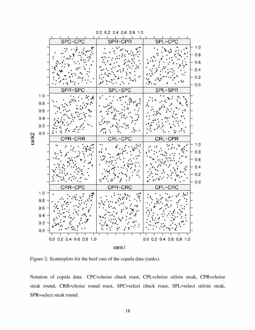
Figure 2: Scatterplots for the beef cuts of the copula data (ranks).

Notation of copula data: CPC=choise chuck roast, CPL=choise sirloin steak, CPR=choise

steak round, CRR=choise round roast, SPC=select chuck roast, SPL=select sirloin steak,

SPR=select steak round.

18

Figure 3: Density plots of parameter estimation from parametric and non-parametric 50,000 boot-

strap repetitions.

Notation of graphs: continuous black curve = parametric bootstrap, dashed read curve = non-

parametric bootstrap, green vertical line = estimated parameter of the original sample, black verti-

cal line = mean of parametric bootstrap, dashed vertical red line = mean of non-parametric boot-

strap.

Notation of copula data: CPC=choise chuck roast, CPL=choise sirloin steak, CPR=choise steak

round, CRR=choise round roast, SPC=select chuck roast, SPL=select sirloin steak, SPR=select

19

Table 1: Copulas functions, parameters, Kendall’s τ , and tail dependence (∗)

Copulas Parameters Kendall’s τ Tail dependence

(λL, λU )

Gaussian θ ∈ (−1,1) 2π

arcsin(θ ) (0,0)

Student − t θ ∈ (−1,1) 2π

arcsin(θ ) 2tν+1(−√

ν +1

√

1−θ

1+θ),

v>2 2tν+1(−√

ν +1

√

1−θ

1+θ)

Clayton θ > 0 θ

θ+2(2

−1θ , 0)

Gumbel θ ≥ 1 1- 1θ

(0, 2 - 21θ )

Frank θ ∈ R\{0} 1 - 4θ+4

D(θ)θ

(0,0)

Joe θ ≥ 1 1+ 4θ 2

∫ 10 tlog(t)(1− t)2(1−θ)/θ dt (0, 2 - 2

1θ )

Gumbel −Clayton θ1 > 0, θ2 ≥ 1 1 - 2θ2(θ1+2) (2

−1θ1θ2 , 2 - 2

1θ2 )

Joe−Clayton θ1 ≥ 1, θ2 > 0 1+ 4θ1θ2

∫ 10 (−(1− (1− t)θ1)θ2+1 (2

−1θ2 , 2 - 2

1θ1 )

*(1−(1−t)θ1 )−θ2−1

(1−t)θ2−1 )dt

(∗) Table from Brechmann and Schepsmeier (2013b).

20

Table 2: Best fitted ARMA(p,q)–GARCH(1,1) models (∗)

Beef Cuts ARMA(p,q)

Choice quality grade

Chuck roast (1,2)

Round roast (2,2)

Steak round (2,2)

Steak sirloin (1,1)

Select quality grade

Chuck roast (2,2)

Steak round (2,2)

Steak sirloin (1,2)

(∗)Application of the Box–Pierce and the autore-

gressive conditional heteroskedasticity–Lagrange

multiplier (ARCH–LM) tests at various lag lengths

showed that residuals are free from autocorrelation

and from ARCH effects.

21

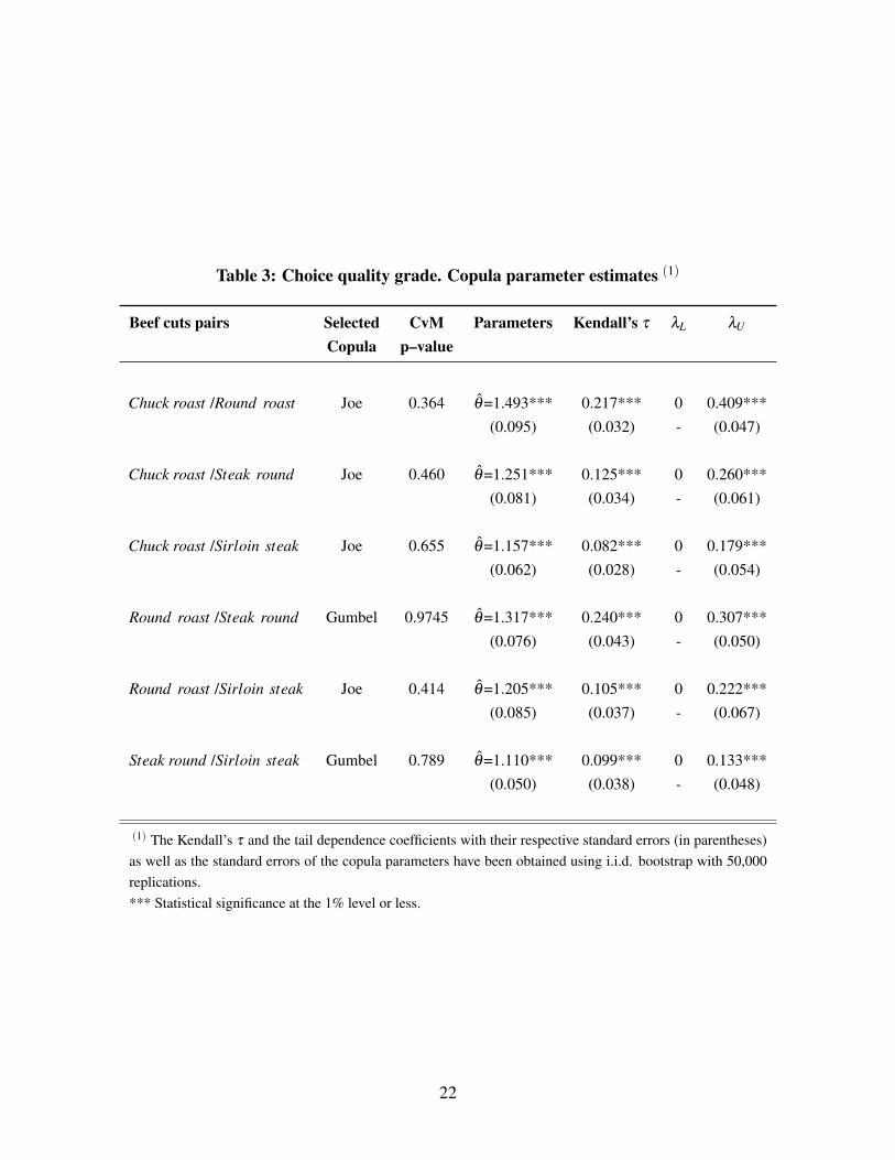
Table 3: Choice quality grade. Copula parameter estimates (1)

Beef cuts pairs Selected CvM Parameters Kendall’s τ λL λU

Copula p–value

Chuck roast /Round roast Joe 0.364 θ=1.493*** 0.217*** 0 0.409***

(0.095) (0.032) - (0.047)

Chuck roast /Steak round Joe 0.460 θ=1.251*** 0.125*** 0 0.260***

(0.081) (0.034) - (0.061)

Chuck roast /Sirloin steak Joe 0.655 θ=1.157*** 0.082*** 0 0.179***

(0.062) (0.028) - (0.054)

Round roast /Steak round Gumbel 0.9745 θ=1.317*** 0.240*** 0 0.307***

(0.076) (0.043) - (0.050)

Round roast /Sirloin steak Joe 0.414 θ=1.205*** 0.105*** 0 0.222***

(0.085) (0.037) - (0.067)

Steak round /Sirloin steak Gumbel 0.789 θ=1.110*** 0.099*** 0 0.133***

(0.050) (0.038) - (0.048)

(1) The Kendall’s τ and the tail dependence coefficients with their respective standard errors (in parentheses)

as well as the standard errors of the copula parameters have been obtained using i.i.d. bootstrap with 50,000

replications.

*** Statistical significance at the 1% level or less.

22

Table 4: Select quality grade. Copula parameter estimates (1)

Beef cuts pairs Selected CvM Parameters Kendall’s τ λL λU

Copula p–value

Chuck roast /Steak round Gaussian 0.363 θ=0.372*** 0.243*** 0 0

(0.059) (0.041) - -

Chuck roast /Sirloin steak Frank 0.672 θ=1.045** 0.115** 0 0

(0.463) (0.049) - -

Steak round/Sirloin steak Frank 0.534 θ=0.864* 0.095* 0 0

(0.511) (0.055) - -

(1) The Kendall’s τ and the tail dependence coefficients with their respective standard errors (in parenthe-

ses) as well as the standard errors of the copula parameters have been obtained using i.i.d. bootstrap with

50,000 replications.

*** Statistical significance at the 1% level or less.

** Statistical significance at the 5% level.

* Statistical significance at the 10% level.

23

Table 5: Choice and Select quality grades. Copula parameter estimates (1)

Pairs between Selected CvM Parameters Kendall’s τ λL λU

Copula p–value

Chuck roast Joe 0.450 θ=1.370*** 0.173*** 0 0.341***

(0.108) (0.039) - (0.063)

Steak round Gaussian 0.977 θ=0.268*** 0.172*** 0 0

(0.062) (0.042) - -

Steak sirloin Gaussian 0.938 θ=0.271*** 0.174*** 0 0

(0.063) (0.042) - -

(1) The Kendall’s τ and the tail dependence coefficients with their respective standard errors (in

parentheses) as well as the standard errors of the copula parameters have been obtained using

i.i.d. bootstrap with 50,000 replications.

*** Statistical significance at the 1% level or less.

24