preventing waste in production: practical methods for ...infohouse.p2ric.org/ref/24/23122.pdf ·...

Preventing waste in production:practical methods for process control

GG

224

This Good Practice Guide was produced by

Envirowise

Prepared with assistance from:

Orr & Boss Ltd

Preventing waste in production:practical methods for process control

Summary

This Good Practice Guide examines various tools and techniques that a company canapply to its production processes in order to save money, improve productivity andproduct quality, and reduce its environmental impact.

The Guide makes extensive use of a fictional example to demonstrate how these tools andtechniques can:

■ help to achieve control and minimise levels of waste;

■ be introduced in a way that encourages their acceptance by staff.

It uses a structured approach that allows a company to:

■ assess the cost of its waste, either using existing company records or by generatingappropriate data;

■ identify the points in a process where waste is arising, assess the specific costs in each caseand present the findings in a format that will encourage action;

■ construct and use simple diagrams to prioritise those process components that are most inneed of attention and, perhaps, change;

■ identify the possible causes of waste, using tools and techniques such as brainstorming, tallysheets, scattergrams, process maps and cause and effect diagrams;

■ carry out a capability study that provides a numerical assessment of how consistent a processis and how well it is meeting the company’s target specifications;

■ identify actions that will improve the process and its capability;

■ use control charts to maintain control once a process is operating satisfactorily.

The Guide, which describes the tools and techniques required and illustrates their application in amanufacturing situation, can be regarded as a blueprint for any company wishing to understandits own processes more fully and minimise process waste. It should be read in conjunction withGood Practice Guide (GG223) Preventing Waste in Production: Industry Examples, which isavailable through the Environment and Energy Helpline on 0800 585794.

Contents

Section Page

1 Introduction 11.1 How this Guide will help you 11.2 Introducing Green and Keen 3

2 What is waste costing you? 52.1 Identifying the problem 52.2 Assessing the costs of waste 6

3 Where is waste arising? 83.1 Establishing a common understanding of the process 83.2 Identifying where waste is occurring 83.3 Assigning costs to the key production processes 83.4 Presenting the findings 9

4 Where should you focus first? 124.1 Plotting a graph to show priorities 124.2 Drawing conclusions and taking the next steps 13

5 What are the possible causes? 145.1 Project 1: leg support production and assembly 145.2 Project 2: bench-top laminating process 16

6 How consistent is your process? 206.1 Introducing the ‘capability’ concept 206.2 Determining the capability of the leg support machining process 20

7 How can your process be improved? 247.1 Actions to improve the performance of the leg support machining process 247.2 Actions to improve the performance of the laminating process 25

8 How can you maintain control? 268.1 The concept of control charts 268.2 Using process control charts to maintain control of the leg support

machining process 268.3 Using process control charts to maintain control of the laminating process 298.4 Control charts: a simple solution 308.5 Further applications 30

9 Further reading 31

Appendices

Appendix 1 Variability 32Appendix 2 Process control charts 38

11

sect

ion

1

Introduction

1.1 How this Guide will help you

This Guide and accompanying Good Practice Guide (GG223) Preventing Waste in Production:Industry Examples1, introduce a range of tools and techniques that use process data to identifyand prevent waste in production processes. Companies that have tackled production waste inthis way have achieved cost savings of up to 1% of turnover.

These savings result from minimising:

■ the excessive consumption of energy or raw materials;

■ losses in the process itself (lost yield and sales);

■ any problems arising when the product is used in a subsequent manufacturing step (reducedyield and possible ‘bottleneck’ difficulties);

■ rejects at the inspection stage;

■ in-service failures.

Although the tools and techniques described in the Guides are based on tried and tested statisticaltechniques, they are straightforward to use and do not require specialist statistical knowledge.

By adopting a similar approach and applying the relevant tools and techniques to its productionprocesses, your company can achieve:

■ cost savings;

■ higher productivity;

■ higher product quality;

■ a lower environmental impact.

This Guide examines a range of tools and techniques that include simple aids for brainstormingand identifying priorities, and the construction of charts based on statistical principles. It uses afictitious manufacturer (Green and Keen) to show how a company can use these approaches toachieve greater control over its production processes, and minimise waste.

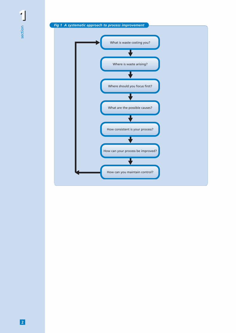
By addressing one or more of the seven stages identified in the Guide (see Fig 1 overleaf) andmaking use of the relevant tools and techniques available, your company can:

■ acquire a better understanding of its processes;

■ analyse process performance and identify areas of avoidable waste;

■ identify opportunities for process improvements;

■ check that any improvements implemented have been effective;

■ ensure that the level of improvement achieved has been maintained.

Furthermore, by reading this Guide alongside GG223, you will be able to see how real companies(see Table 1 overleaf) have benefited from this approach.

1 GG223 is available free of charge through the Environment and Energy Helpline on freephone 0800 585794.

11se

ctio

n

2

Where is waste arising?

Where should you focus first?

What are the possible causes?

How consistent is your process?

How can your process be improved?

How can you maintain control?

What is waste costing you?

Fig 1 A systematic approach to process improvement

11

sect

ion

3

1.2 Introducing Green and Keen

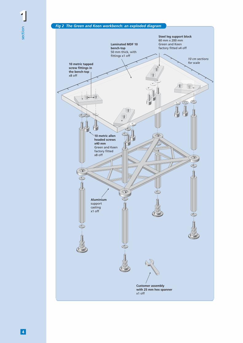
Green and Keen manufactures a relatively heavy-duty, flat-pack, self-assembly workbench (seeFig 2 overleaf). It buys the basic bench-tops, which incorporate tapped fittings for the legsupports. In-house manufacturing operations consist of laminating these bench-tops andproducing machined leg supports that are assembled into each bench-top.

The company employs 22 staff and has an annual turnover of about £990 000, based on theproduction and sale of 11 000 workbenches at £89.99 each.

✓ ✓ ✓ ✓ ✓ ✓ ✓ ✓ ✓ ✓

✓

✓ ✓ ✓ ✓

✓ ✓ ✓

✓

✓ ✓ ✓ ✓ ✓

✓

✓

✓

✓

✓ ✓

✓ ✓ ✓

✓

1 2 3 4 5 6 7 8 9 10


Basic production data collection


Process mapping/flow chart


Histograms

Pareto diagrams


‘Fishbone’ diagrams

Experiments/investigations


Normal variability

Special variability

Capability assessment

How can your process be improved?

Rechecking capability


Control charts

Other

Operator training

Automatic mixer control

Pers

torp

Ltd

Furn

itu

re m

anu

fact

ure

C S

hip

pam

Ltd

Foo

d p

aste

s/fi

llin

g

Tran

spri

nts

Ltd

Prin

tin

g t

exti

les

tran

sfer

pap

er

Edin

bu

rgh

Cry

stal

Gla

ssw

are

man

ufa

ctu

re

No

vem

Car

inte

rio

r (w

oo

den

ven

eers

)

Illb

ruck

Ko

ike

Gen

eral

ru

bb

er g

oo

ds

Mit

ex G

lass

Fib

re L

tdW

ove

n g

lass

fib

re

BFF

No

nw

ove

ns

No

n-w

ove

n s

pec

ialis

t fa

bri

cs

Fen

ner

Co

nve

yor

Bel

tin

gC

om

po

site

co

nve

yor

bel

ts

Co

rus

Fou

nd

ryIr

on

cas

tin

g

Table 1 Techniques employed by the Industry Example companies to achieve theiraims (see GG223)

11se

ctio

n

4

Steel leg support block60 mm x 200 mmGreen and Keenfactory fitted x4 off

10 cm sectionsfor scale

10 metric allenheaded screwsx40 mmGreen and Keenfactory fitted x8 off

Customer assemblywith 25 mm hex spannerx1 off

Aluminiumsupportcastingx1 off

10 metric tappedscrew fittings inthe bench-topx8 off

Laminated MDF 10bench-top50 mm thick, with fittings x1 off

Fig 2 The Green and Keen workbench: an exploded diagram

22

sect

ion

5


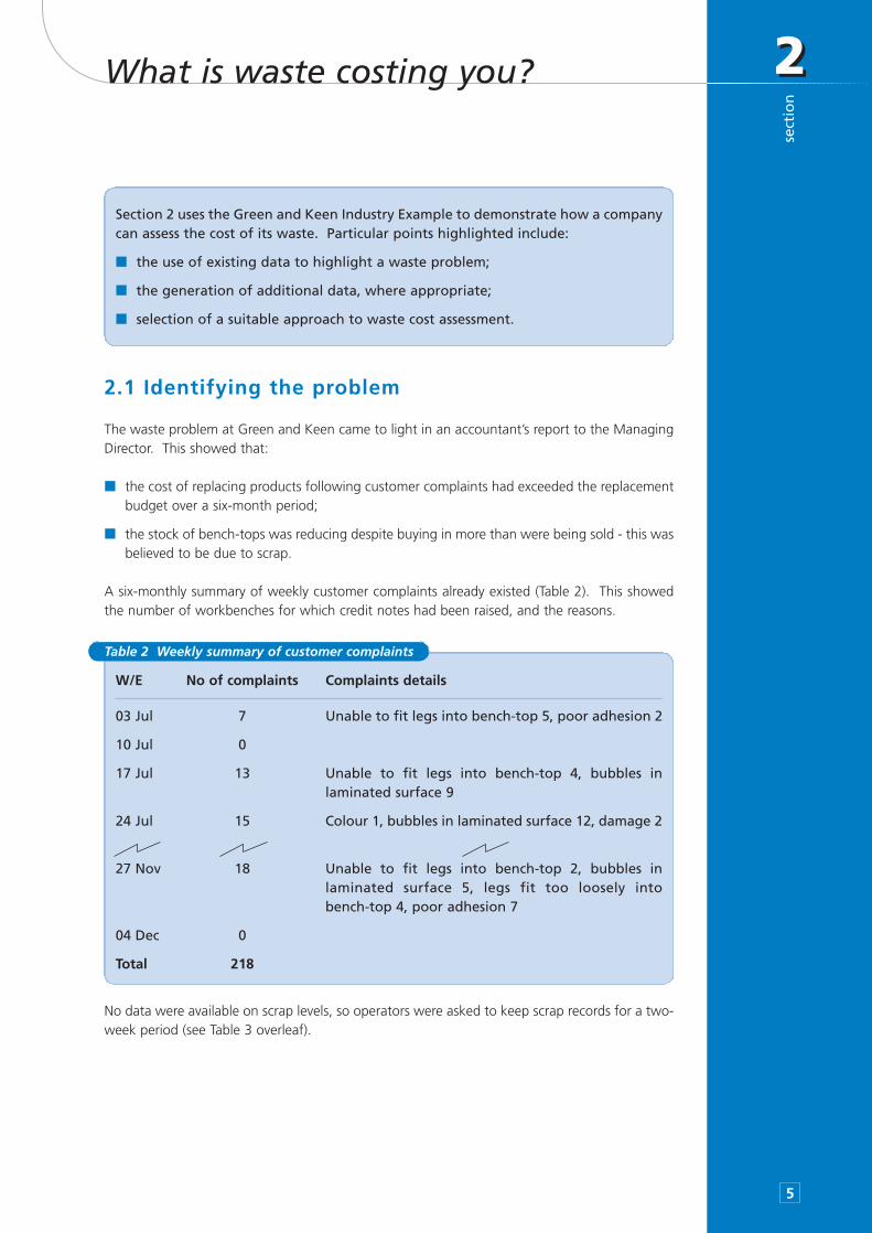
2.1 Identifying the problem

The waste problem at Green and Keen came to light in an accountant’s report to the ManagingDirector. This showed that:

■ the cost of replacing products following customer complaints had exceeded the replacementbudget over a six-month period;

■ the stock of bench-tops was reducing despite buying in more than were being sold - this wasbelieved to be due to scrap.

A six-monthly summary of weekly customer complaints already existed (Table 2). This showedthe number of workbenches for which credit notes had been raised, and the reasons.

No data were available on scrap levels, so operators were asked to keep scrap records for a two-week period (see Table 3 overleaf).

Section 2 uses the Green and Keen Industry Example to demonstrate how a companycan assess the cost of its waste. Particular points highlighted include:

■ the use of existing data to highlight a waste problem;

■ the generation of additional data, where appropriate;

■ selection of a suitable approach to waste cost assessment.

W/E No of complaints Complaints details

03 Jul 7 Unable to fit legs into bench-top 5, poor adhesion 2

10 Jul 0

17 Jul 13 Unable to fit legs into bench-top 4, bubbles inlaminated surface 9

24 Jul 15 Colour 1, bubbles in laminated surface 12, damage 2

27 Nov 18 Unable to fit legs into bench-top 2, bubbles inlaminated surface 5, legs fit too loosely into bench-top 4, poor adhesion 7

04 Dec 0

Total 218

Table 2 Weekly summary of customer complaints

22se

ctio

n

6

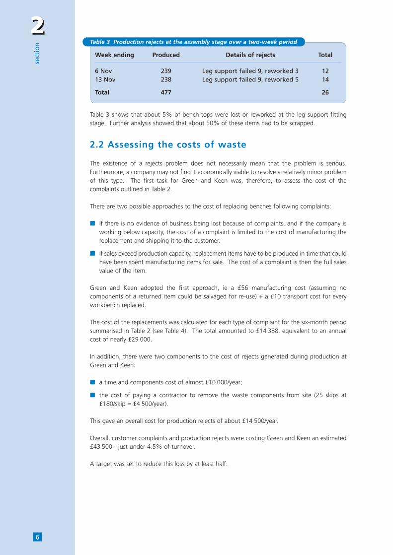
Table 3 shows that about 5% of bench-tops were lost or reworked at the leg support fittingstage. Further analysis showed that about 50% of these items had to be scrapped.

2.2 Assessing the costs of waste

The existence of a rejects problem does not necessarily mean that the problem is serious.Furthermore, a company may not find it economically viable to resolve a relatively minor problemof this type. The first task for Green and Keen was, therefore, to assess the cost of thecomplaints outlined in Table 2.

There are two possible approaches to the cost of replacing benches following complaints:

■ If there is no evidence of business being lost because of complaints, and if the company isworking below capacity, the cost of a complaint is limited to the cost of manufacturing thereplacement and shipping it to the customer.

■ If sales exceed production capacity, replacement items have to be produced in time that couldhave been spent manufacturing items for sale. The cost of a complaint is then the full salesvalue of the item.

Green and Keen adopted the first approach, ie a £56 manufacturing cost (assuming nocomponents of a returned item could be salvaged for re-use) + a £10 transport cost for everyworkbench replaced.

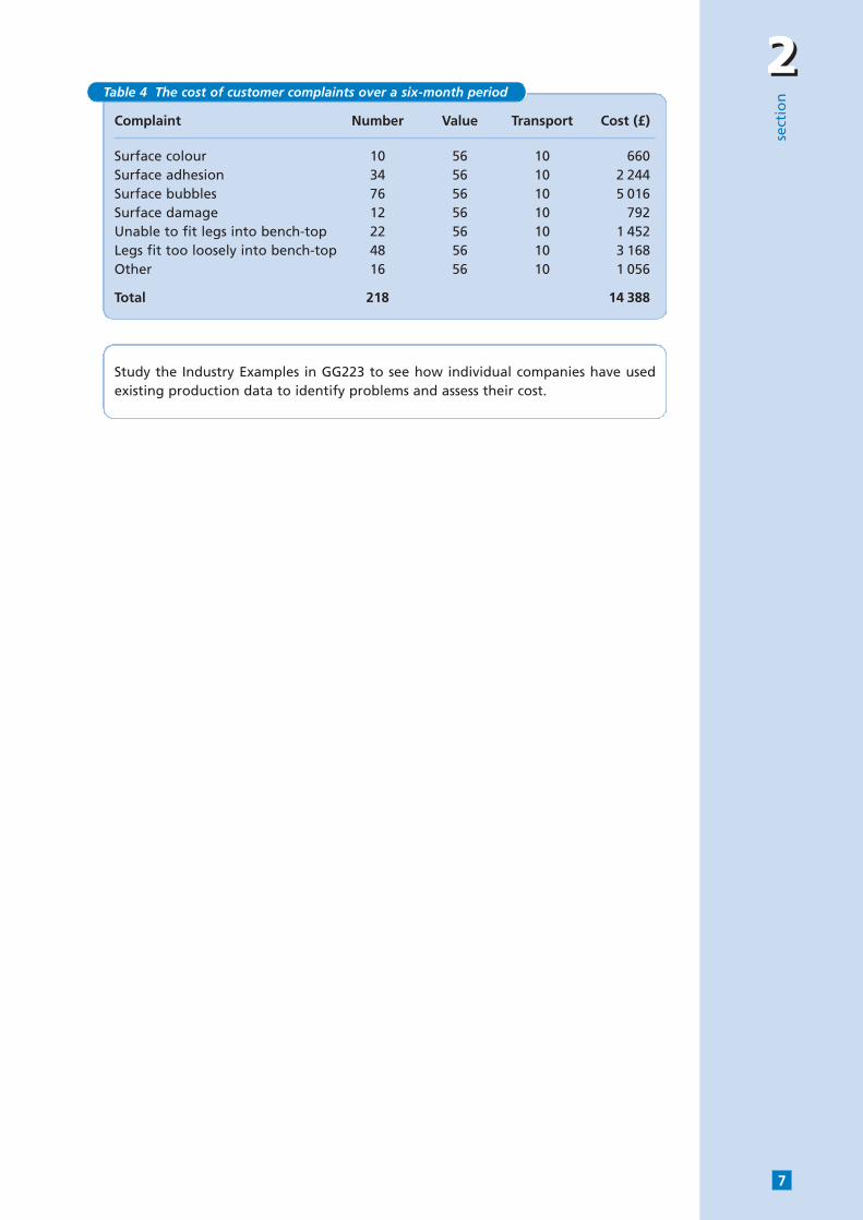
The cost of the replacements was calculated for each type of complaint for the six-month periodsummarised in Table 2 (see Table 4). The total amounted to £14 388, equivalent to an annualcost of nearly £29 000.

In addition, there were two components to the cost of rejects generated during production atGreen and Keen:

■ a time and components cost of almost £10 000/year;

■ the cost of paying a contractor to remove the waste components from site (25 skips at£180/skip = £4 500/year).

This gave an overall cost for production rejects of about £14 500/year.

Overall, customer complaints and production rejects were costing Green and Keen an estimated£43 500 - just under 4.5% of turnover.

A target was set to reduce this loss by at least half.

Week ending Produced Details of rejects Total

6 Nov 239 Leg support failed 9, reworked 3 1213 Nov 238 Leg support failed 9, reworked 5 14

Total 477 26

Table 3 Production rejects at the assembly stage over a two-week period

22

sect

ion

7

Complaint Number Value Transport Cost (£)

Surface colour 10 56 10 660Surface adhesion 34 56 10 2 244Surface bubbles 76 56 10 5 016Surface damage 12 56 10 792Unable to fit legs into bench-top 22 56 10 1 452Legs fit too loosely into bench-top 48 56 10 3 168Other 16 56 10 1 056

Total 218 14 388

Table 4 The cost of customer complaints over a six-month period

Study the Industry Examples in GG223 to see how individual companies have usedexisting production data to identify problems and assess their cost.

33se

ctio

n

8


3.1 Establishing a common understanding of theprocess

To establish where waste is arising in a process it is necessary to have an accurate and agreedunderstanding of that process. One way of achieving this is to ask a member of staff - possibly theProduction Director - to produce a rough flow chart of the process and to discuss its content withother relevant staff such as process operators and accounts staff. The regular production meetingmay be an appropriate time for a ‘brainstorming’ or discussion session to ensure agreement.

When this approach was adopted at Green and Keen it became evident that different staffviewed the production process from a slightly different perspective. There were no basictechnical disagreements, but there were differences in emphasis. Those attending theproduction meeting paid a visit to the production area, after which agreement was quicklyreached on the key processes (eg cutting and drilling metal, assembling components) and on theorder of production. The findings were noted on a flip-chart.

3.2 Identifying where waste is occurring

The next step is to identify those parts of the process where waste is occurring. Initially, a broad-brush approach is more appropriate than a detailed analysis. That can come later (see Section 5).

At Green and Keen, the production meeting demonstrated that there was no shortage of ideasbut that operators had strong (and conflicting) opinions about which parts of the process wereto blame for the rejects. By insisting on a broad-brush approach, the Production Director wasable to obtain an initial ‘feel’ for how often lost time, and reject and assembly problems occurredat key stages in the process. This was noted on the flip-chart.

3.3 Assigning costs to the key production processes

The third step is to assign approximate costs to the key components of the production process.To achieve this, it may be appropriate to invite relevant members of the accounts staff to theproduction meeting.

At Green and Keen, the accounts staff proved useful in focusing the discussion so thatappropriate costs could be assigned. Many of the process operators were previously unaware ofthese costs.

Section 3 shows how you can identify the point in your process where waste isarising. This Section will demonstrate:

■ the need for a common understanding of the process as a basis for identifying themain sources of waste;

■ the value of involving accounts staff when assigning costs to the variouscomponents of the process;

■ how you can present the findings in a suitable format, eg flow chart and table.

33

sect

ion

9

3.4 Presenting the findings

It is essential to present the findings in a format that will subsequently be useful. The ProductionDirector at Green and Keen adopted two formats:

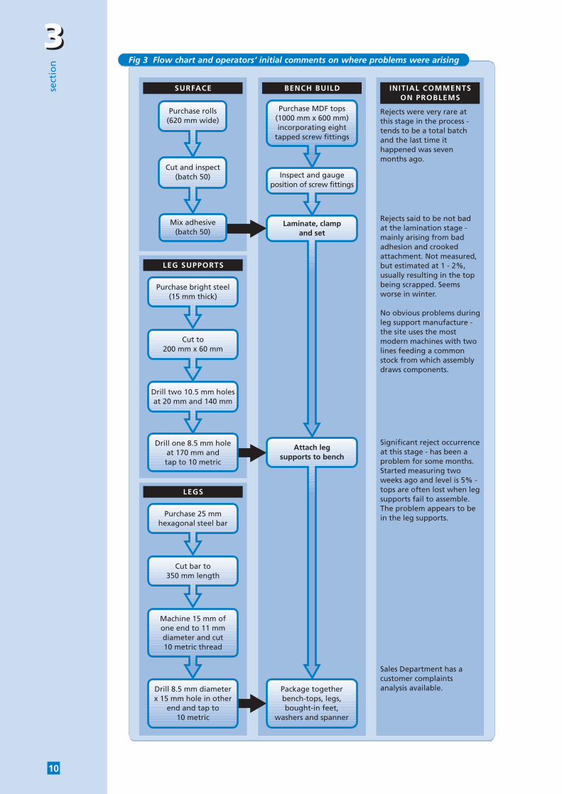
■ a flow chart, designed using a software package and showing operators’ initial comments onwhere the problems were arising (see Fig 3 overleaf);

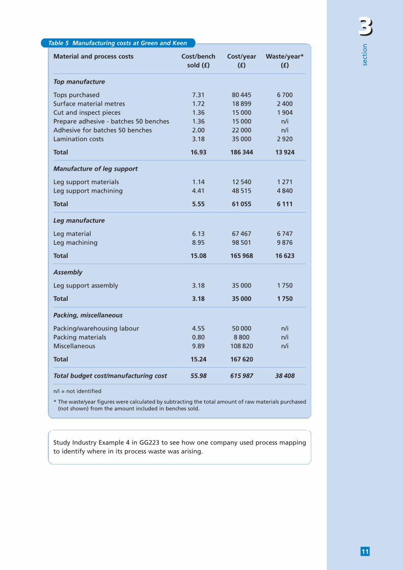
■ a table of costs (see Table 5 overleaf).

The flow chart provided the basis for more detailed process flow charts in the main problem areas.

Table 5 proved valuable in that:

■ It showed clearly the difference in cost between a fault resulting in the loss of an expensivebench-top and one resulting in the loss of a relatively inexpensive leg support.

■ It also confirmed the overall high cost of wasted production. Over £38 000 was beingwasted each year due to the issues of customer returns, leg-support assembly scrap andother causes. This does not include the cost of shipping the customer returns (nearly £4 400)or skip charges (£4 500); the total cost was probably over £47 000. This calculation producesa result that is within 10% of the initial estimate given in Section 2.2, which was based onlimited data (ie production rejects over two weeks and customer complaints over six months).

33se

ctio

n

10

SURFACE BENCH BU ILD INIT IAL COMMENTSON PROBLEMS

Purchase rolls(620 mm wide)

Cut and inspect(batch 50)

LEG SUPPORTS

Purchase bright steel(15 mm thick)

Drill two 10.5 mm holesat 20 mm and 140 mm

Cut to200 mm x 60 mm

LEGS

Purchase 25 mmhexagonal steel bar

Machine 15 mm ofone end to 11 mmdiameter and cut10 metric thread

Purchase MDF tops(1000 mm x 600 mm)incorporating eight

tapped screw fittings

Cut bar to350 mm length

Inspect and gaugeposition of screw fittings

Laminate, clampand set

Attach legsupports to bench

Package togetherbench-tops, legs,bought-in feet,

washers and spanner

Mix adhesive(batch 50)

Drill one 8.5 mm holeat 170 mm andtap to 10 metric

Drill 8.5 mm diameterx 15 mm hole in other

end and tap to10 metric

Rejects were very rare atthis stage in the process -tends to be a total batchand the last time ithappened was sevenmonths ago.

Rejects said to be not badat the lamination stage -mainly arising from badadhesion and crookedattachment. Not measured,but estimated at 1 - 2%,usually resulting in the topbeing scrapped. Seemsworse in winter.

No obvious problems duringleg support manufacture -the site uses the mostmodern machines with twolines feeding a commonstock from which assemblydraws components.

Significant reject occurrenceat this stage - has been aproblem for some months.Started measuring twoweeks ago and level is 5% -tops are often lost when legsupports fail to assemble.The problem appears to bein the leg supports.

Sales Department has acustomer complaintsanalysis available.

Fig 3 Flow chart and operators’ initial comments on where problems were arising

33

sect

ion

11

Material and process costs Cost/bench Cost/year Waste/year*sold (£) (£) (£)

Top manufacture

Tops purchased 7.31 80 445 6 700Surface material metres 1.72 18 899 2 400Cut and inspect pieces 1.36 15 000 1 904Prepare adhesive - batches 50 benches 1.36 15 000 n/iAdhesive for batches 50 benches 2.00 22 000 n/iLamination costs 3.18 35 000 2 920

Total 16.93 186 344 13 924

Manufacture of leg support

Leg support materials 1.14 12 540 1 271Leg support machining 4.41 48 515 4 840

Total 5.55 61 055 6 111

Leg manufacture

Leg material 6.13 67 467 6 747Leg machining 8.95 98 501 9 876

Total 15.08 165 968 16 623

Assembly

Leg support assembly 3.18 35 000 1 750

Total 3.18 35 000 1 750

Packing, miscellaneous

Packing/warehousing labour 4.55 50 000 n/iPacking materials 0.80 8 800 n/iMiscellaneous 9.89 108 820 n/i

Total 15.24 167 620

Total budget cost/manufacturing cost 55.98 615 987 38 408

n/i = not identified

* The waste/year figures were calculated by subtracting the total amount of raw materials purchased(not shown) from the amount included in benches sold.

Table 5 Manufacturing costs at Green and Keen

Study Industry Example 4 in GG223 to see how one company used process mappingto identify where in its process waste was arising.

44se

ctio

n

12


4.1 Plotting a graph to show priorities

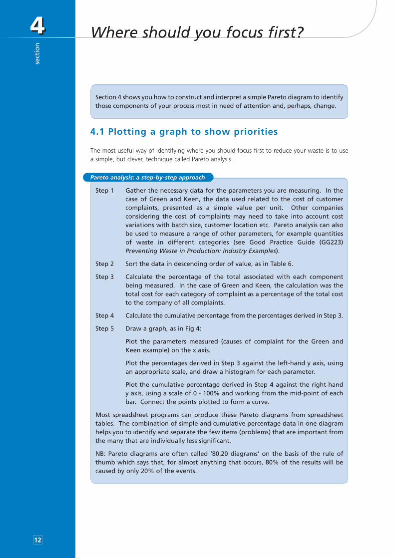
The most useful way of identifying where you should focus first to reduce your waste is to usea simple, but clever, technique called Pareto analysis.

Section 4 shows you how to construct and interpret a simple Pareto diagram to identifythose components of your process most in need of attention and, perhaps, change.

Step 1 Gather the necessary data for the parameters you are measuring. In thecase of Green and Keen, the data used related to the cost of customercomplaints, presented as a simple value per unit. Other companiesconsidering the cost of complaints may need to take into account costvariations with batch size, customer location etc. Pareto analysis can alsobe used to measure a range of other parameters, for example quantitiesof waste in different categories (see Good Practice Guide (GG223)Preventing Waste in Production: Industry Examples).

Step 2 Sort the data in descending order of value, as in Table 6.

Step 3 Calculate the percentage of the total associated with each componentbeing measured. In the case of Green and Keen, the calculation was thetotal cost for each category of complaint as a percentage of the total costto the company of all complaints.

Step 4 Calculate the cumulative percentage from the percentages derived in Step 3.

Step 5 Draw a graph, as in Fig 4:

Plot the parameters measured (causes of complaint for the Green andKeen example) on the x axis.

Plot the percentages derived in Step 3 against the left-hand y axis, usingan appropriate scale, and draw a histogram for each parameter.

Plot the cumulative percentage derived in Step 4 against the right-hand y axis, using a scale of 0 - 100% and working from the mid-point of eachbar. Connect the points plotted to form a curve.

Most spreadsheet programs can produce these Pareto diagrams from spreadsheettables. The combination of simple and cumulative percentage data in one diagramhelps you to identify and separate the few items (problems) that are important fromthe many that are individually less significant.

NB: Pareto diagrams are often called ‘80:20 diagrams’ on the basis of the rule ofthumb which says that, for almost anything that occurs, 80% of the results will becaused by only 20% of the events.

Pareto analysis: a step-by-step approach

44

sect

ion

13

4.2 Drawing conclusions and taking the next steps

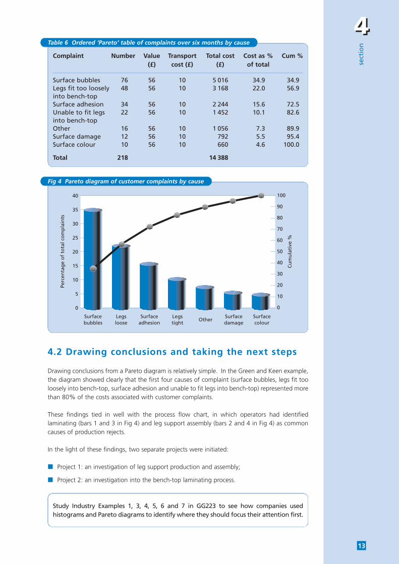
Drawing conclusions from a Pareto diagram is relatively simple. In the Green and Keen example,the diagram showed clearly that the first four causes of complaint (surface bubbles, legs fit tooloosely into bench-top, surface adhesion and unable to fit legs into bench-top) represented morethan 80% of the costs associated with customer complaints.

These findings tied in well with the process flow chart, in which operators had identifiedlaminating (bars 1 and 3 in Fig 4) and leg support assembly (bars 2 and 4 in Fig 4) as commoncauses of production rejects.

In the light of these findings, two separate projects were initiated:

■ Project 1: an investigation of leg support production and assembly;

■ Project 2: an investigation into the bench-top laminating process.

Complaint Number Value Transport Total cost Cost as % Cum %(£) cost (£) (£) of total

Surface bubbles 76 56 10 5 016 34.9 34.9Legs fit too loosely 48 56 10 3 168 22.0 56.9into bench-topSurface adhesion 34 56 10 2 244 15.6 72.5Unable to fit legs 22 56 10 1 452 10.1 82.6into bench-topOther 16 56 10 1 056 7.3 89.9Surface damage 12 56 10 792 5.5 95.4Surface colour 10 56 10 660 4.6 100.0

Total 218 14 388

Table 6 Ordered ‘Pareto’ table of complaints over six months by cause

40

35

30

25

20

15

10

5

0

100

90

80

70

60

50

40

30

20

10

0

Perc

enta

ge

of

tota

l co

mp

lain

ts

Cu

mu

lati

ve %

Surfacebubbles

Legsloose

Surfaceadhesion

Legstight

Surfacedamage

Surfacecolour

Other

Fig 4 Pareto diagram of customer complaints by cause

Study Industry Examples 1, 3, 4, 5, 6 and 7 in GG223 to see how companies usedhistograms and Pareto diagrams to identify where they should focus their attention first.

55se

ctio

n

14


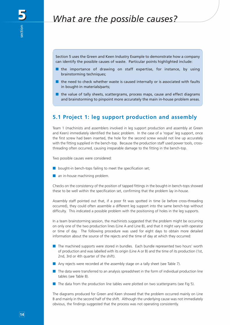
5.1 Project 1: leg support production and assembly

Team 1 (machinists and assemblers involved in leg support production and assembly at Greenand Keen) immediately identified the basic problem. In the case of a ‘rogue’ leg support, oncethe first screw had been inserted, the hole for the second screw would not line up accuratelywith the fitting supplied in the bench-top. Because the production staff used power tools, cross-threading often occurred, causing irreparable damage to the fitting in the bench-top.

Two possible causes were considered:

■ bought-in bench-tops failing to meet the specification set;

■ an in-house machining problem.

Checks on the consistency of the position of tapped fittings in the bought-in bench-tops showedthese to be well within the specification set, confirming that the problem lay in-house.

Assembly staff pointed out that, if a poor fit was spotted in time (ie before cross-threadingoccurred), they could often assemble a different leg support into the same bench-top withoutdifficulty. This indicated a possible problem with the positioning of holes in the leg supports.

In a team brainstorming session, the machinists suggested that the problem might be occurringon only one of the two production lines (Line A and Line B), and that it might vary with operatoror time of day. The following procedure was used for eight days to obtain more detailedinformation about the source of the rejects and the time of day at which they occurred:

■ The machined supports were stored in bundles. Each bundle represented two hours’ worthof production and was labelled with its origin (Line A or B) and the time of its production (1st,2nd, 3rd or 4th quarter of the shift).

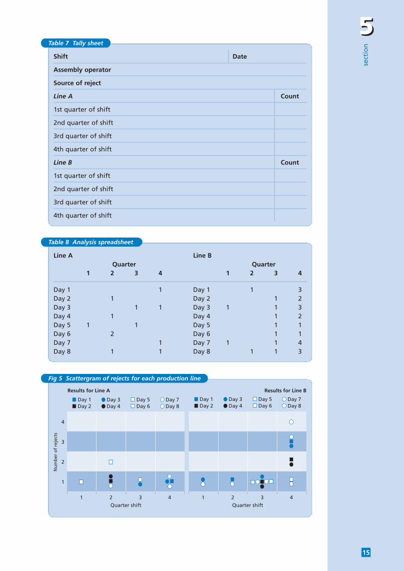
■ Any rejects were recorded at the assembly stage on a tally sheet (see Table 7).

■ The data were transferred to an analysis spreadsheet in the form of individual production linetables (see Table 8).

■ The data from the production line tables were plotted on two scattergrams (see Fig 5).

The diagrams produced for Green and Keen showed that the problem occurred mainly on LineB and mainly in the second half of the shift. Although the underlying cause was not immediatelyobvious, the findings suggested that the process was not operating consistently.

Section 5 uses the Green and Keen Industry Example to demonstrate how a companycan identify the possible causes of waste. Particular points highlighted include:

■ the importance of drawing on staff expertise, for instance, by usingbrainstorming techniques;

■ the need to check whether waste is caused internally or is associated with faultsin bought-in materials/parts;

■ the value of tally sheets, scattergrams, process maps, cause and effect diagramsand brainstorming to pinpoint more accurately the main in-house problem areas.

55

sect

ion

15

Shift Date

Assembly operator

Source of reject

Line A Count

1st quarter of shift

2nd quarter of shift

3rd quarter of shift

4th quarter of shift

Line B Count

1st quarter of shift

2nd quarter of shift

3rd quarter of shift

4th quarter of shift

Table 7 Tally sheet

Line A Line BQuarter Quarter

1 2 3 4 1 2 3 4

Day 1 1 Day 1 1 3Day 2 1 Day 2 1 2Day 3 1 1 Day 3 1 1 3Day 4 1 Day 4 1 2Day 5 1 1 Day 5 1 1Day 6 2 Day 6 1 1Day 7 1 Day 7 1 1 4Day 8 1 1 Day 8 1 1 3

Table 8 Analysis spreadsheet

Day 1Day 2

Day 3Day 4

Day 5Day 6

Day 7Day 8

Day 1Day 2

Day 3Day 4

Day 5Day 6

Day 7Day 8

4

3

2

1

Nu

mb

er o

f re

ject

s

1 2 3 4

Quarter shift

1 2 3 4

Quarter shift

Results for Line A Results for Line B

Fig 5 Scattergram of rejects for each production line

55se

ctio

n

16

5.2 Project 2: bench-top laminating process

5.2.1 Defining the problem

The Pareto diagram in Section 4 had already shown that surface bubbles were the main causeof the costs arising from customer complaints (34.9%), with surface adhesion also being asignificant problem (15.6%).

Team 2 (staff responsible for glue preparation, veneer cutting and laminating) was certain thatboth laminating and assembly staff would notice obvious defects and would scrap any defectivebench-tops before they left the factory. Its first task was, therefore, to inspect the rejects anddetermine the nature of the defects.

5.2.2 Identifying the causes

Team 2 initially thought that the problems might be developing several days after laminating,while the glue was drying out and curing. The glue was either failing completely or producinggas: possible reasons included a faulty batch of glue, a dirty surface or the effect of moisturecontent.

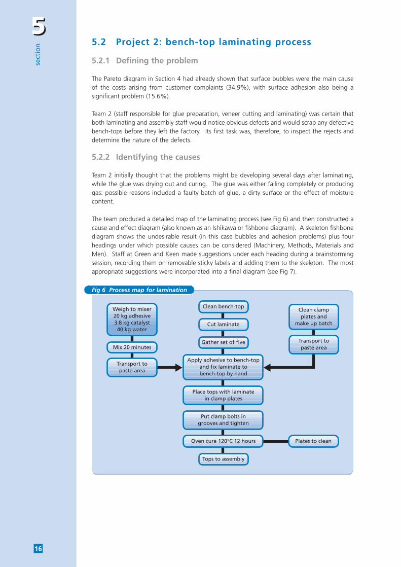
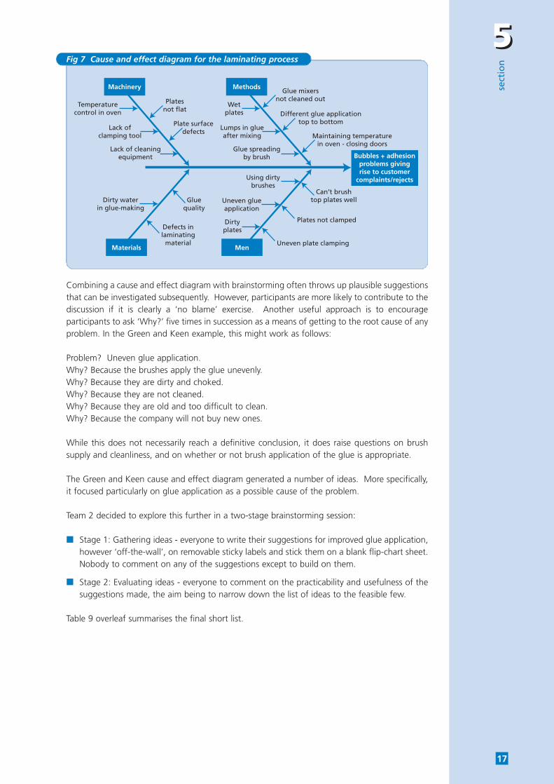
The team produced a detailed map of the laminating process (see Fig 6) and then constructed acause and effect diagram (also known as an Ishikawa or fishbone diagram). A skeleton fishbonediagram shows the undesirable result (in this case bubbles and adhesion problems) plus fourheadings under which possible causes can be considered (Machinery, Methods, Materials andMen). Staff at Green and Keen made suggestions under each heading during a brainstormingsession, recording them on removable sticky labels and adding them to the skeleton. The mostappropriate suggestions were incorporated into a final diagram (see Fig 7).

Clean bench-top

Cut laminate

Gather set of five

Tops to assembly

Apply adhesive to bench-topand fix laminate tobench-top by hand

Place tops with laminatein clamp plates

Put clamp bolts ingrooves and tighten

Oven cure 120°C 12 hours Plates to clean

Clean clampplates and

make up batch

Weigh to mixer20 kg adhesive3.8 kg catalyst40 kg water

Mix 20 minutes

Transport topaste area

Transport topaste area

Fig 6 Process map for lamination

55

sect

ion

17

Combining a cause and effect diagram with brainstorming often throws up plausible suggestionsthat can be investigated subsequently. However, participants are more likely to contribute to thediscussion if it is clearly a ‘no blame’ exercise. Another useful approach is to encourageparticipants to ask ‘Why?’ five times in succession as a means of getting to the root cause of anyproblem. In the Green and Keen example, this might work as follows:

Problem? Uneven glue application.Why? Because the brushes apply the glue unevenly.Why? Because they are dirty and choked.Why? Because they are not cleaned.Why? Because they are old and too difficult to clean.Why? Because the company will not buy new ones.

While this does not necessarily reach a definitive conclusion, it does raise questions on brushsupply and cleanliness, and on whether or not brush application of the glue is appropriate.

The Green and Keen cause and effect diagram generated a number of ideas. More specifically,it focused particularly on glue application as a possible cause of the problem.

Team 2 decided to explore this further in a two-stage brainstorming session:

■ Stage 1: Gathering ideas - everyone to write their suggestions for improved glue application,however ‘off-the-wall’, on removable sticky labels and stick them on a blank flip-chart sheet.Nobody to comment on any of the suggestions except to build on them.

■ Stage 2: Evaluating ideas - everyone to comment on the practicability and usefulness of thesuggestions made, the aim being to narrow down the list of ideas to the feasible few.

Table 9 overleaf summarises the final short list.

Machinery Methods

Materials Men

Bubbles + adhesionproblems givingrise to customer

complaints/rejects

Dirty waterin glue-making

Temperaturecontrol in oven

Lack of cleaningequipment

Lack ofclamping tool

Wetplates

Glue spreadingby brush

Lumps in glueafter mixing

Platesnot flat

Plate surfacedefects

Defects inlaminating

material

Glue mixersnot cleaned out

Different glue applicationtop to bottom

Maintaining temperaturein oven - closing doors

Gluequality

Using dirtybrushes

Dirtyplates

Uneven glueapplication

Can’t brushtop plates well

Plates not clamped

Uneven plate clamping

Fig 7 Cause and effect diagram for the laminating process

55se

ctio

n

18

5.2.3 Backing up the suggestions with data

The Green and Keen Production Director decided to back up Team 2’s suggestions with somerelevant data. He was particularly interested in assessing two possibilities:

■ whether the position of the laminating plate was affecting glue spreading and the formationof bubbles;

■ whether early signs of bubble formation might be present at the assembly stage or when thelaminated tops were removed from the clamps, even though the full problem might notdevelop for several days.

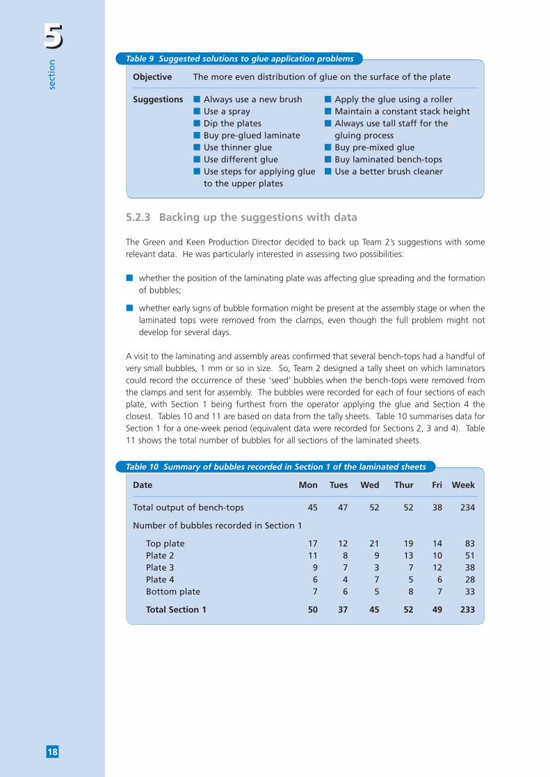
A visit to the laminating and assembly areas confirmed that several bench-tops had a handful ofvery small bubbles, 1 mm or so in size. So, Team 2 designed a tally sheet on which laminatorscould record the occurrence of these ‘seed’ bubbles when the bench-tops were removed fromthe clamps and sent for assembly. The bubbles were recorded for each of four sections of eachplate, with Section 1 being furthest from the operator applying the glue and Section 4 theclosest. Tables 10 and 11 are based on data from the tally sheets. Table 10 summarises data forSection 1 for a one-week period (equivalent data were recorded for Sections 2, 3 and 4). Table11 shows the total number of bubbles for all sections of the laminated sheets.

Objective The more even distribution of glue on the surface of the plate

Suggestions ■ Always use a new brush ■ Apply the glue using a roller■ Use a spray ■ Maintain a constant stack height■ Dip the plates ■ Always use tall staff for the■ Buy pre-glued laminate gluing process■ Use thinner glue ■ Buy pre-mixed glue■ Use different glue ■ Buy laminated bench-tops■ Use steps for applying glue ■ Use a better brush cleaner

to the upper plates

Table 9 Suggested solutions to glue application problems

Date Mon Tues Wed Thur Fri Week

Total output of bench-tops 45 47 52 52 38 234

Number of bubbles recorded in Section 1

Top plate 17 12 21 19 14 83Plate 2 11 8 9 13 10 51Plate 3 9 7 3 7 12 38Plate 4 6 4 7 5 6 28Bottom plate 7 6 5 8 7 33

Total Section 1 50 37 45 52 49 233

Table 10 Summary of bubbles recorded in Section 1 of the laminated sheets

55

sect

ion

19

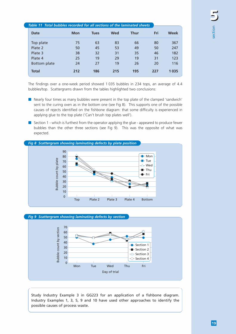
The findings over a one-week period showed 1 035 bubbles in 234 tops, an average of 4.4bubbles/top. Scattergrams drawn from the tables highlighted two conclusions:

■ Nearly four times as many bubbles were present in the top plate of the clamped ‘sandwich’sent to the curing oven as in the bottom one (see Fig 8). This supports one of the possiblecauses of rejects identified on the fishbone diagram: that some difficulty is experienced inapplying glue to the top plate (‘Can’t brush top plates well’).

■ Section 1 - which is furthest from the operator applying the glue - appeared to produce fewerbubbles than the other three sections (see Fig 9). This was the opposite of what wasexpected.



Total 212 186 215 195 227 1 035

Table 11 Total bubbles recorded for all sections of the laminated sheets

MonTueWedThuFri

Top Plate 2 Plate 3 Plate 4 Bottom

90

80

70

60

50

40

30

20

10

0

Bu

bb

le c

ou

nt

by

pla

te

Fig 8 Scattergram showing laminating defects by plate position

Section 1Section 2Section 3Section 4

70

60

50

40

30

20

10

0Bu

bb

le c

ou

nt

by

sect

ion

Mon Tue Wed Thu Fri

Day of trial

Fig 9 Scattergram showing laminating defects by section

Study Industry Example 3 in GG223 for an application of a fishbone diagram.Industry Examples 1, 3, 5, 9 and 10 have used other approaches to identify thepossible causes of process waste.

66se

ctio

n

20


6.1 Introducing the ‘capability’ concept

Where a process component, eg a machining line, is not operating consistently, it is useful tocarry out a capability assessment of that component.

Industrial companies usually set target specifications (or tolerances) for key attributes of theirproducts, ie they specify the highest and lowest values that are acceptable. These specificationswill depend on the level of consistency and accuracy required. The capability of a process is ameasure of how well it can meet the specifications set. It determines the percentage of productsrejected for being outside the specifications. A capable process is one that can meet the end-use specification most of the time. The more variable a process is, the less capable it will be.

To determine the capability of a process, it is important to understand some simple, but important,statistical concepts relating to variability and how it is measured. The most important of these arerange, standard deviation and capability indexes. These are explained in Appendix 1.

Capability assessments can provide:

■ confirmation of the possible cause of a problem;

■ an immediate measure of production line performance - instead of waiting for rejects at theassembly stage;

■ an accurate performance base-line against which future changes can be measured;

■ a first step towards the rapid identification of subsequent process inconsistencies usingcontrol charts.

6.2 Determining the capability of the leg supportmachining process

Team 1 had already confirmed (see Section 5.1) that the incoming bench-tops were within thespecification set, ie with leg support screw fitting centres 120 mm apart ± 0.1 mm. Checks werealso made on:

■ internal gauge capability;

■ the process specification.

The results of these checks were as follows:

■ The gauging methods used internally to measure the holes in bench-tops and leg supportsagreed with those used by the bench-top supplier.

Section 6 introduces the concept of process capability - a measure of how well aprocess is meeting the target specifications set by the industry concerned.

It then uses the Green and Keen Industry Example to calculate and interpret twocapability values for each production line - the capability each line could achieve ifit were correctly centred, and its capability in practice.

66

sect

ion

21

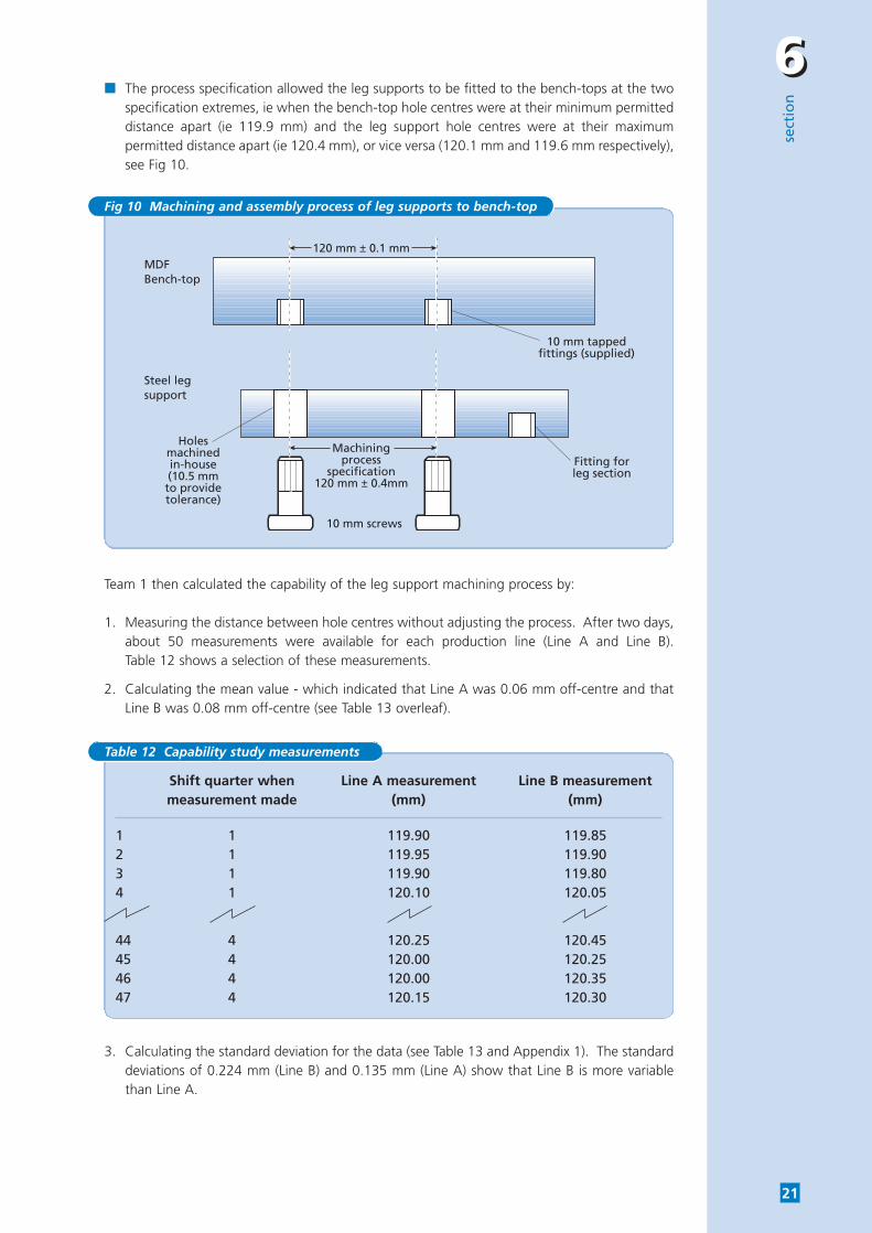
■ The process specification allowed the leg supports to be fitted to the bench-tops at the twospecification extremes, ie when the bench-top hole centres were at their minimum permitteddistance apart (ie 119.9 mm) and the leg support hole centres were at their maximumpermitted distance apart (ie 120.4 mm), or vice versa (120.1 mm and 119.6 mm respectively),see Fig 10.

Team 1 then calculated the capability of the leg support machining process by:

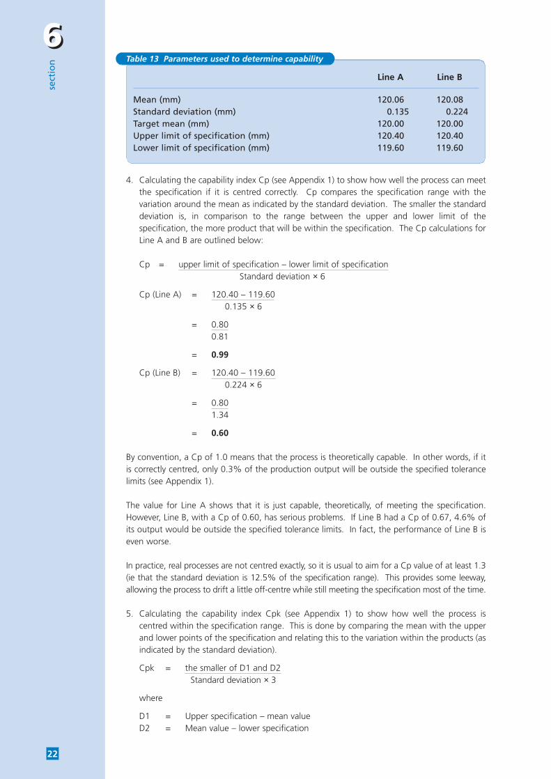
1. Measuring the distance between hole centres without adjusting the process. After two days,about 50 measurements were available for each production line (Line A and Line B). Table 12 shows a selection of these measurements.

2. Calculating the mean value - which indicated that Line A was 0.06 mm off-centre and thatLine B was 0.08 mm off-centre (see Table 13 overleaf).

3. Calculating the standard deviation for the data (see Table 13 and Appendix 1). The standarddeviations of 0.224 mm (Line B) and 0.135 mm (Line A) show that Line B is more variablethan Line A.

MDFBench-top

Steel legsupport

10 mm screws

120 mm ± 0.1 mm

Machiningprocess

specification120 mm ± 0.4mm

Holesmachinedin-house(10.5 mmto providetolerance)

10 mm tappedfittings (supplied)

Fitting forleg section

Fig 10 Machining and assembly process of leg supports to bench-top

Shift quarter when Line A measurement Line B measurement measurement made (mm) (mm)

1 1 119.90 119.852 1 119.95 119.903 1 119.90 119.804 1 120.10 120.05

44 4 120.25 120.4545 4 120.00 120.2546 4 120.00 120.3547 4 120.15 120.30

Table 12 Capability study measurements

66se

ctio

n

22

4. Calculating the capability index Cp (see Appendix 1) to show how well the process can meetthe specification if it is centred correctly. Cp compares the specification range with thevariation around the mean as indicated by the standard deviation. The smaller the standarddeviation is, in comparison to the range between the upper and lower limit of thespecification, the more product that will be within the specification. The Cp calculations forLine A and B are outlined below:

Cp = upper limit of specification – lower limit of specification Standard deviation × 6

Cp (Line A) = 120.40 – 119.60 0.135 × 6

= 0.800.81

= 0.99

Cp (Line B) = 120.40 – 119.600.224 × 6

= 0.801.34

= 0.60

By convention, a Cp of 1.0 means that the process is theoretically capable. In other words, if itis correctly centred, only 0.3% of the production output will be outside the specified tolerancelimits (see Appendix 1).

The value for Line A shows that it is just capable, theoretically, of meeting the specification.However, Line B, with a Cp of 0.60, has serious problems. If Line B had a Cp of 0.67, 4.6% ofits output would be outside the specified tolerance limits. In fact, the performance of Line B iseven worse.

In practice, real processes are not centred exactly, so it is usual to aim for a Cp value of at least 1.3(ie that the standard deviation is 12.5% of the specification range). This provides some leeway,allowing the process to drift a little off-centre while still meeting the specification most of the time.

5. Calculating the capability index Cpk (see Appendix 1) to show how well the process iscentred within the specification range. This is done by comparing the mean with the upperand lower points of the specification and relating this to the variation within the products (asindicated by the standard deviation).

Cpk = the smaller of D1 and D2Standard deviation × 3

where

D1 = Upper specification – mean valueD2 = Mean value – lower specification

Line A Line B

Mean (mm) 120.06 120.08Standard deviation (mm) 0.135 0.224Target mean (mm) 120.00 120.00Upper limit of specification (mm) 120.40 120.40Lower limit of specification (mm) 119.60 119.60

Table 13 Parameters used to determine capability

66

sect

ion

23

Line A

D1 = 120.40 – 120.06= 0.34 mm

D2 = 120.06 – 119.60= 0.46 mm

Cpk = 0.340.41

= 0.83

Line B

D1 = 120.40 – 120.08= 0.32 mm

D2 = 120.08 – 119.60= 0.48 mm

Cpk = 0.320.67

= 0.48

By convention, a Cpk of 1.0 means that the process is reasonably well centred, however,increasing Cpk above 1.0 will further reduce the number of products not meeting thespecification.

It is clear from these values that Line A is performing below its theoretical capability because itis off-centre. Every measured value that is more than 0.83 × three standard deviations (ie 2.49standard deviations) above the measured mean will be out of specification. Statistical tablesindicate that this represents a rejects level of towards 1%.

Line B is performing worse, with a Cpk of 0.48. Statistical calculations and tables suggest thatabout 8% of the output of this production line will be above the upper specification limit. LineB also experiences a significant deterioration later in each day.

As indicated for Cp, the preferred value for Cpk for both lines is usually closer to 1.3, the valueat which they would easily meet process specifications and keep scrap levels to a minimum.

Having performed these calculations, Team 1 understood the following:

■ the low value of Cpk meant that the lines were not performing satisfactorily and actionneeded to be taken;

■ the low value of Cp for Line B suggested that there was one or more causes of significantvariability in the line;

■ the off-target means (causing a lower value of Cpk than Cp) being present on both Line Aand B indicated that there may have been a second factor causing this problem;

■ the current values of Cp and Cpk against which to measure future improvement were 0.99and 0.83 for Line A and 0.60 and 0.48 for Line B.

Study Industry Example 2 in GG223 to show how one company undertook acapability assessment of its process.

77se

ctio

n

24

How can your process beimproved?

7.1 Actions to improve the performance of the legsupport machining process

Where a Production Director identifies a poor process capability (see Section 6), the obvious wayforward is to focus first on the main areas of poor performance. In the Green and Keen IndustryExample, Line B is obviously performing very badly.

It is also worth considering whether performance that is potentially ‘acceptable’, as Line A wouldbe if correctly centred (ie has a higher Cpk), could nevertheless be improved by making simpleengineering modifications.

The first action taken at Green and Keen was a maintenance check of production Line B. Thischeck identified:

■ a bearing that was overheating and on the point of collapse;

■ badly worn drill guides.

Both were immediately replaced, and the line was then run for a couple of days, with checks ontemperature and vibration. The drill bearings on Line A were also changed as a precautionarymeasure.

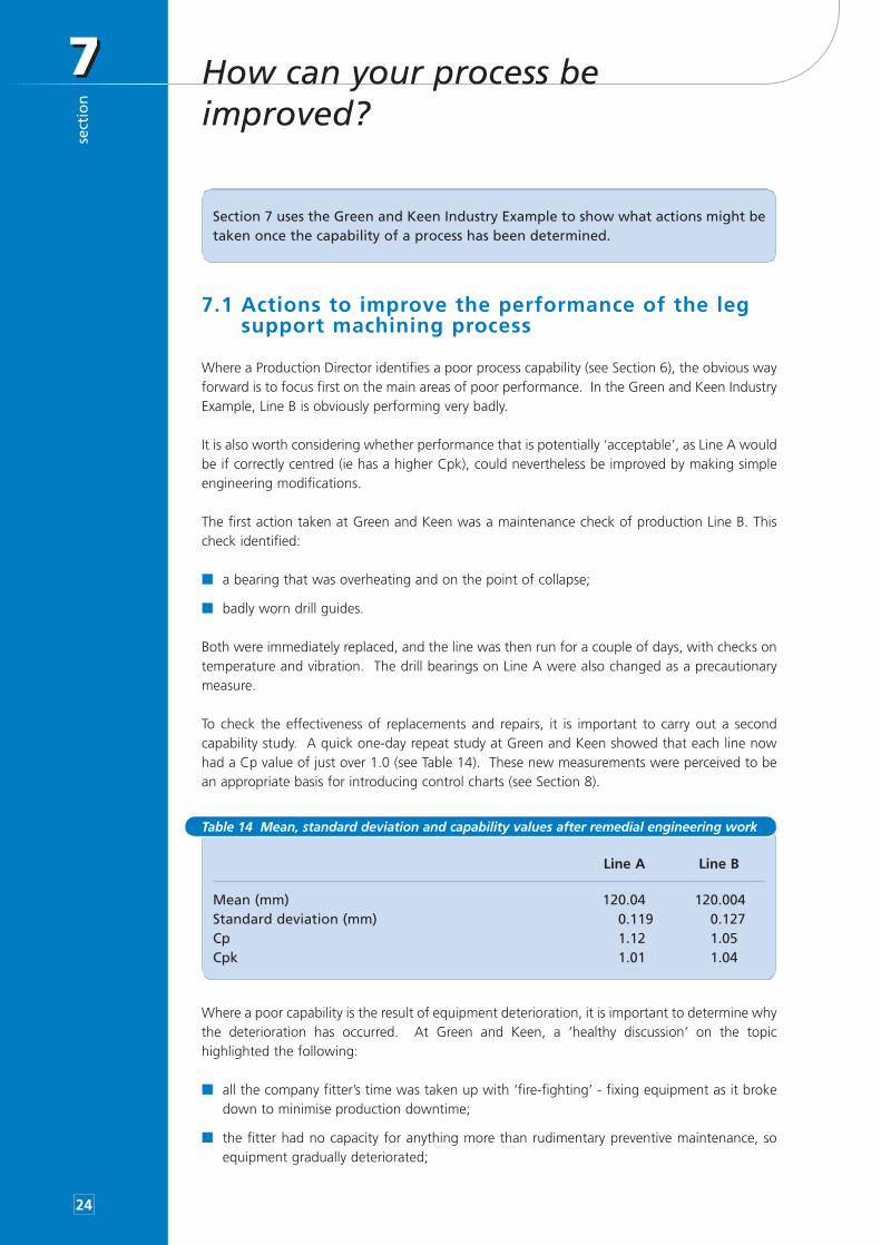
To check the effectiveness of replacements and repairs, it is important to carry out a secondcapability study. A quick one-day repeat study at Green and Keen showed that each line nowhad a Cp value of just over 1.0 (see Table 14). These new measurements were perceived to bean appropriate basis for introducing control charts (see Section 8).

Where a poor capability is the result of equipment deterioration, it is important to determine whythe deterioration has occurred. At Green and Keen, a ‘healthy discussion’ on the topichighlighted the following:

■ all the company fitter’s time was taken up with ‘fire-fighting’ - fixing equipment as it brokedown to minimise production downtime;

■ the fitter had no capacity for anything more than rudimentary preventive maintenance, soequipment gradually deteriorated;

Line A Line B

Mean (mm) 120.04 120.004Standard deviation (mm) 0.119 0.127Cp 1.12 1.05Cpk 1.01 1.04

Table 14 Mean, standard deviation and capability values after remedial engineering work

Section 7 uses the Green and Keen Industry Example to show what actions might betaken once the capability of a process has been determined.

77

sect

ion

25

■ time spent maintaining the machining lines reduced the time spent keeping the laminatingoven operational.

7.2 Actions to improve the performance of thelaminating process

The progress made in identifying the causes of the laminating problems at Green and Keen (seeSection 5.2) encouraged the introduction of two major changes:

■ modifications to the bench and working position so that all plates are at a convenient heightfor coating with glue;

■ improvements to the arrangements for glue mixing and plate cleaning.

A subsequent spot check showed that these changes had reduced the level of ‘seed’ bubbles bya factor of two, to about two per bench-top. This was expected to give a similar level ofreduction in customer complaints.

However, the laminating team believed that further improvements could be achieved. It set upexperiments on glue viscosity, glue application techniques and curing conditions and, as a resultof the findings, introduced a number of further changes and improvements. (The design andconduct of experiments is covered in some of the books listed in Section 9.)

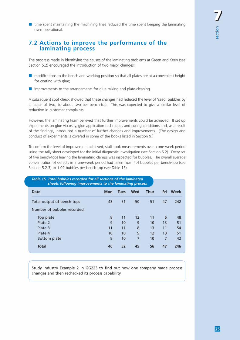
To confirm the level of improvement achieved, staff took measurements over a one-week periodusing the tally sheet developed for the initial diagnostic investigation (see Section 5.2). Every setof five bench-tops leaving the laminating clamps was inspected for bubbles. The overall averageconcentration of defects in a one-week period had fallen from 4.4 bubbles per bench-top (seeSection 5.2.3) to 1.02 bubbles per bench-top (see Table 15).


Total output of bench-tops 43 51 50 51 47 242

Number of bubbles recorded


Total 46 52 45 56 47 246

Table 15 Total bubbles recorded for all sections of the laminatedsheets following improvements to the laminating process

Study Industry Example 2 in GG223 to find out how one company made processchanges and then rechecked its process capability.

88se

ctio

n

26


8.1 The concept of control charts

Where remedial work improves the capability of a process, it is essential to remember that lowreject levels will be maintained only if there is no deterioration in the equipment used and if theoperators maintain the control settings correctly.

It may be possible to initiate procedures that include the recording of rejects on tally sheets orencouraging machinists to look out for problems and adjust the machines accordingly. This typeof approach has its disadvantages:

■ once parts are rejected, waste has been incurred;

■ machinists may make unnecessary changes to machines or methods.

Another option is to use control charts, which are simple both to construct and to use. Theprocedure is as follows:

1. Take a significant number of measurements from the process.

2. Use simple equations to calculate an Upper Control Limit (UCL), a Lower Control Limit (LCL)and a Centre Line (CL).

3. Draw on a chart the three horizontal lines that correspond to the UCL, LCL and CL values.The difference between the upper and lower control limits indicates the normal variation tobe expected.

4. Regularly measure and plot the performance of the process on the chart.

If the measured value stays well within the two boundary lines (UCL and LCL) and shows noparticular trend, your process is under control and you need not take any action.

If the measured values gradually move away from the CL towards one of the limits or passes oneof the limits, this may indicate that your process needs attention.

There are several types of process control chart, each plotting slightly different variables and eachusing different statistical rules to calculate the LCL, CL and UCL values. Further details are givenin Appendix 2.

8.2 Using process control charts to maintain controlof the leg support machining process

The Green and Keen Production Director introduced the ‘x-bar R’ chart as a means ofmaintaining control of the leg support machining process. The x-bar R chart is really twoseparate charts, one for plotting the mean value and one for plotting the range.

Section 8 introduces the concept of control charts to maintain control once a processis operating satisfactorily. It then uses data from the Green and Keen Industry Exampleto construct two types of control chart and explains how each should be interpreted.

88

sect

ion

27

The procedure required is as follows:

1. Take small samples of measurements at regular intervals.

2. Calculate the mean value (x-bar) of the measurements in each sample.

3. Calculate the range of values measured (the difference between the largest and the smallestmeasurement in each sample).

4. Plot each result on an ‘x-bar R’ chart.

Certain decisions also have to be made at the start:

■ How large a sample should be taken?

■ How often should sampling take place?

■ Where should the control limits be set?

It is important to remember that, although increasing the sample size improves accuracy, moretime is involved in taking that sample.

At Green and Keen, it was agreed that samples would be taken twice each day (during the firstand last quarters of a shift) with four measurements taken per sample - a level that would givea reasonable indication of any changes taking place.

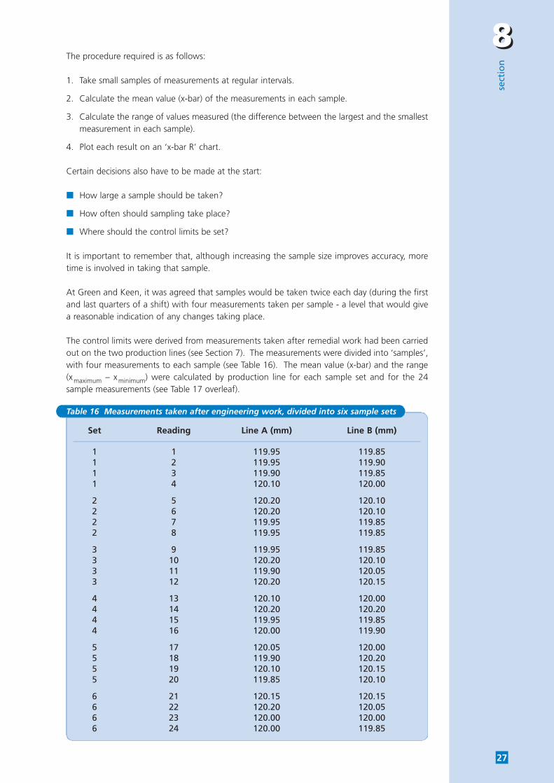
The control limits were derived from measurements taken after remedial work had been carriedout on the two production lines (see Section 7). The measurements were divided into ‘samples’,with four measurements to each sample (see Table 16). The mean value (x-bar) and the range(xmaximum – xminimum) were calculated by production line for each sample set and for the 24sample measurements (see Table 17 overleaf).

Set Reading Line A (mm) Line B (mm)

1 1 119.95 119.851 2 119.95 119.901 3 119.90 119.851 4 120.10 120.00

2 5 120.20 120.102 6 120.20 120.102 7 119.95 119.852 8 119.95 119.85

3 9 119.95 119.853 10 120.20 120.103 11 119.90 120.053 12 120.20 120.15

4 13 120.10 120.004 14 120.20 120.204 15 119.95 119.854 16 120.00 119.90

5 17 120.05 120.005 18 119.90 120.205 19 120.10 120.155 20 119.85 120.10

6 21 120.15 120.156 22 120.20 120.056 23 120.00 120.006 24 120.00 119.85

Table 16 Measurements taken after engineering work, divided into six sample sets

88se

ctio

n

28

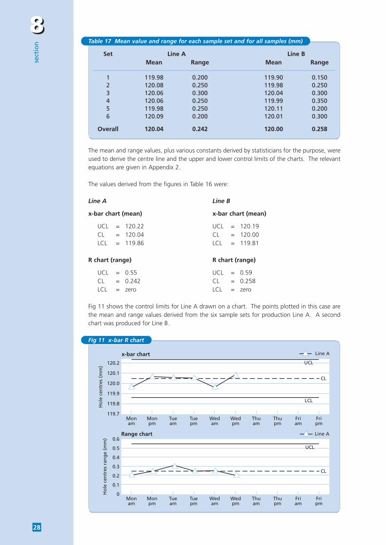
The mean and range values, plus various constants derived by statisticians for the purpose, wereused to derive the centre line and the upper and lower control limits of the charts. The relevantequations are given in Appendix 2.

The values derived from the figures in Table 16 were:

Line A Line B

x-bar chart (mean) x-bar chart (mean)

UCL = 120.22 UCL = 120.19CL = 120.04 CL = 120.00LCL = 119.86 LCL = 119.81

R chart (range) R chart (range)

UCL = 0.55 UCL = 0.59CL = 0.242 CL = 0.258LCL = zero LCL = zero

Fig 11 shows the control limits for Line A drawn on a chart. The points plotted in this case arethe mean and range values derived from the six sample sets for production Line A. A secondchart was produced for Line B.

Set Line A Line BMean Range Mean Range

1 119.98 0.200 119.90 0.1502 120.08 0.250 119.98 0.2503 120.06 0.300 120.04 0.3004 120.06 0.250 119.99 0.3505 119.98 0.250 120.11 0.2006 120.09 0.200 120.01 0.300

Overall 120.04 0.242 120.00 0.258

Table 17 Mean value and range for each sample set and for all samples (mm)

Monam

Monpm

Tueam

Tuepm

Wedam

Wedpm

Thuam

Thupm

Friam

Fripm

Monam

Monpm

Tueam

Tuepm

Wedam

Wedpm

Thuam

Thupm

Friam

Fripm

UCL

CL

LCL

UCL

CL

120.2

120.1

120.0

119.9

119.8

119.7

0.6

0.5

0.4

0.3

0.2

0.1

0

Ho

le c

entr

es (

mm

)H

ole

cen

tres

ran

ge

(mm

)

x-bar chart

Range chart

Line A

Line A

Fig 11 x-bar R chart

88

sect

ion

29

Chart interpretation can be summarised as follows:

■ Where the plotted x-bar results fall between the upper and lower limits, no significant changeis taking place within the process. In this example, this means that the mean distancebetween holes is not altering significantly.

■ Any overall trend up or down on the graph indicates a methodical drift away from a centredprocess, even if the range chart stays within the control limits set.

■ If the plotted range results hit the upper limit, the process is becoming more erratic. Even ifthe mean stays on target, some items will be outside the specification set.

■ The combination of drift and a more erratic process indicates a deterioration in processcapability and should initiate remedial action.

8.3 Using process control charts to maintain controlof the laminating process

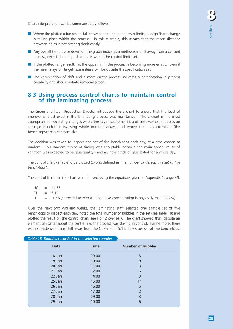
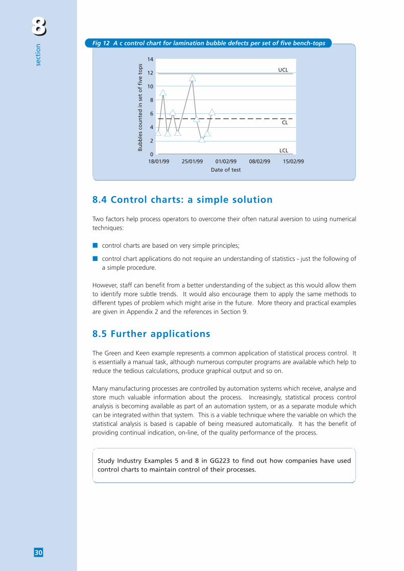
The Green and Keen Production Director introduced the c chart to ensure that the level ofimprovement achieved in the laminating process was maintained. The c chart is the mostappropriate for recording changes where the key measurement is a discrete variable (bubbles ona single bench-top) involving whole number values, and where the units examined (the bench-tops) are a constant size.

The decision was taken to inspect one set of five bench-tops each day, at a time chosen atrandom. This random choice of timing was acceptable because the main special cause ofvariation was expected to be glue quality - and a single batch of glue lasted for a whole day.

The control chart variable to be plotted (c) was defined as ‘the number of defects in a set of fivebench-tops’.

The control limits for the chart were derived using the equations given in Appendix 2, page 43:

UCL = 11.88CL = 5.10LCL = -1.68 (corrected to zero as a negative concentration is physically meaningless)

Over the next two working weeks, the laminating staff selected one sample set of five bench-tops to inspect each day, noted the total number of bubbles in the set (see Table 18) andplotted the result on the control chart (see Fig 12 overleaf). The chart showed that, despite anelement of scatter about the centre line, the process was staying in control. Furthermore, therewas no evidence of any drift away from the CL value of 5.1 bubbles per set of five bench-tops.

Date Time Number of bubbles

18 Jan 09:00 319 Jan 10:00 920 Jan 11:00 321 Jan 12:00 622 Jan 14:00 325 Jan 15:00 1126 Jan 16:00 527 Jan 17:00 228 Jan 09:00 329 Jan 10:00 6

Table 18 Bubbles recorded in the selected samples

88se

ctio

n

30

8.4 Control charts: a simple solution

Two factors help process operators to overcome their often natural aversion to using numericaltechniques:

■ control charts are based on very simple principles;

■ control chart applications do not require an understanding of statistics - just the following ofa simple procedure.

However, staff can benefit from a better understanding of the subject as this would allow themto identify more subtle trends. It would also encourage them to apply the same methods todifferent types of problem which might arise in the future. More theory and practical examplesare given in Appendix 2 and the references in Section 9.

8.5 Further applications

The Green and Keen example represents a common application of statistical process control. Itis essentially a manual task, although numerous computer programs are available which help toreduce the tedious calculations, produce graphical output and so on.

Many manufacturing processes are controlled by automation systems which receive, analyse andstore much valuable information about the process. Increasingly, statistical process controlanalysis is becoming available as part of an automation system, or as a separate module whichcan be integrated within that system. This is a viable technique where the variable on which thestatistical analysis is based is capable of being measured automatically. It has the benefit ofproviding continual indication, on-line, of the quality performance of the process.

14

12

10

8

6

4

2

0

Bu

bb

les

cou

nte

d in

set

of

five

to

ps

UCL

CL

LCL

18/01/99 25/01/99 01/02/99 08/02/99 15/02/99

Date of test

Fig 12 A c control chart for lamination bubble defects per set of five bench-tops

Study Industry Examples 5 and 8 in GG223 to find out how companies have usedcontrol charts to maintain control of their processes.

99

sect

ion

31

Further reading

SPC Simplified: Practical Steps to Quality by Amsden, Butler and Amsden. Published by QualityResources. ISBN 0-527-91617-X

Histograms, SPC, brainstorming, cause and effect. Very little theory or statistics but lots ofgood examples.

Statistical Process Control (SPC). Published by Chrysler, Ford and General Motors.This is how you must do it as a supplier to these three motor industry majors. Copies fromCarwin Continuous Ltd, Unit 1 Trade Link, Western Avenue, West Thurrock, Grays, EssexRM20 3FJ (Tel: 01708 861333). This forms a part of the set of books that make up the guidesto QS9000 motor industry certification.

Statistics for Experimenters by Box, Hunter and Hunter. Published by John Wiley. ISBN 0-471-09315-7

A heavyweight, detailed book on this subject.

100 Methods for Total Quality Management by Kanji & Asher. ISBN 0-8039-7747-6Defines and describes minimally most of the quality acronyms and techniques. Excellentbibliography and good references to many of the techniques contained in the text. Not adetailed ‘how to do it’ guide.

Improving Competitiveness through Control. Published by the DTI’s Advanced ControlTechnology Transfer (ACTT) Programme.

This guide introduces statistical process control and a variety of other process controltechniques and how they can be used. Available free-of-charge from the DTI (Tel: 020 72151344, Fax: 020 7215 1518).

Statistical Process Control, 3rd Edition by John S Oakland. Published by Butterworth Heinmann,21 May 1999. ISBN 0-750-64439-7.

This text provides the foundations of good quality management and process control, coveringall theory and techniques. Also available in hardback.

11ap

pen

dix

32

Variability

The theory

If you try to repeat something exactly several times, you will find that the results of each attemptare not exactly the same - although the differences may be small. Variability is, therefore, inevitable.

There are two main causes of variability:

■ ‘normal’ or ‘common’ causes, which are a random feature of the world we live in and arebeyond our control;

■ ‘special’ or ‘assignable’ causes, which are individually significant or identifiable.

Recognising the difference between these two types of cause is an important part of getting thebest results. Common causes can be reduced only by identifying the inherent limitations of themanufacturing process, and ways to improve accuracy. Special causes can be reduced byidentifying the change or process failure and implementing rapid corrective action.

Normal and specialcauses of variation

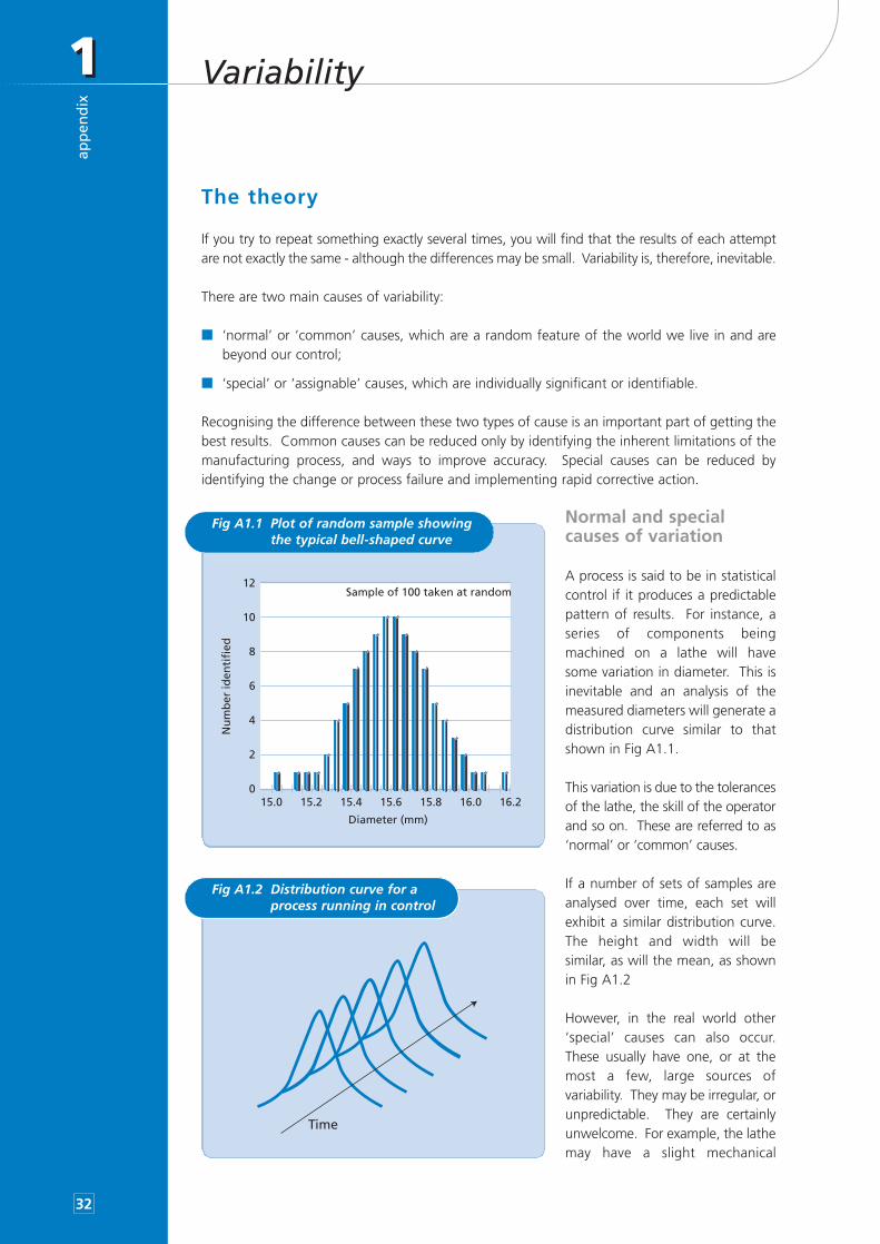
A process is said to be in statisticalcontrol if it produces a predictablepattern of results. For instance, aseries of components beingmachined on a lathe will havesome variation in diameter. This isinevitable and an analysis of themeasured diameters will generate adistribution curve similar to thatshown in Fig A1.1.

This variation is due to the tolerancesof the lathe, the skill of the operatorand so on. These are referred to as‘normal’ or ‘common’ causes.

If a number of sets of samples areanalysed over time, each set willexhibit a similar distribution curve.The height and width will besimilar, as will the mean, as shownin Fig A1.2

However, in the real world other‘special’ causes can also occur.These usually have one, or at themost a few, large sources ofvariability. They may be irregular, orunpredictable. They are certainlyunwelcome. For example, the lathemay have a slight mechanical

12

10

8

6

4

2

0

Nu

mb

er id

enti

fied

Sample of 100 taken at random

Diameter (mm)

15.0 15.2 15.4 15.6 15.8 16.0 16.2

Fig A1.1 Plot of random sample showingthe typical bell-shaped curve

Time

Fig A1.2 Distribution curve for aprocess running in control

11

app

end

ix

33

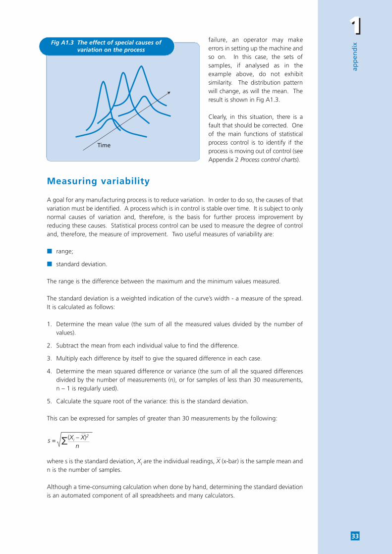
failure, an operator may makeerrors in setting up the machine andso on. In this case, the sets ofsamples, if analysed as in theexample above, do not exhibitsimilarity. The distribution patternwill change, as will the mean. Theresult is shown in Fig A1.3.

Clearly, in this situation, there is afault that should be corrected. Oneof the main functions of statisticalprocess control is to identify if theprocess is moving out of control (seeAppendix 2 Process control charts).

Measuring variability

A goal for any manufacturing process is to reduce variation. In order to do so, the causes of thatvariation must be identified. A process which is in control is stable over time. It is subject to onlynormal causes of variation and, therefore, is the basis for further process improvement byreducing these causes. Statistical process control can be used to measure the degree of controland, therefore, the measure of improvement. Two useful measures of variability are:

■ range;

■ standard deviation.

The range is the difference between the maximum and the minimum values measured.

The standard deviation is a weighted indication of the curve’s width - a measure of the spread.It is calculated as follows:

1. Determine the mean value (the sum of all the measured values divided by the number ofvalues).

2. Subtract the mean from each individual value to find the difference.

3. Multiply each difference by itself to give the squared difference in each case.

4. Determine the mean squared difference or variance (the sum of all the squared differencesdivided by the number of measurements (n), or for samples of less than 30 measurements, n – 1 is regularly used).

5. Calculate the square root of the variance: this is the standard deviation.

This can be expressed for samples of greater than 30 measurements by the following:

where s is the standard deviation, Xi are the individual readings, X (x-bar) is the sample mean andn is the number of samples.

Although a time-consuming calculation when done by hand, determining the standard deviationis an automated component of all spreadsheets and many calculators.

Time

Fig A1.3 The effect of special causes ofvariation on the process

s = Σ(Xi – X)2

n

11ap

pen

dix

34

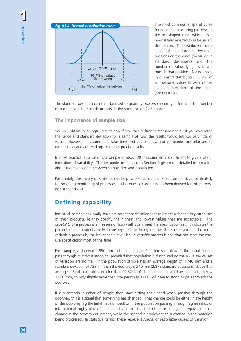
The most common shape of curvefound in manufacturing processes isthe bell-shaped curve which has anormal (also referred to as Gaussian)distribution. This distribution has astatistical relationship betweenpositions on the curve (measured instandard deviations) and thenumber of values lying inside andoutside that position. For example,in a normal distribution, 99.7% ofall measured values lie within threestandard deviations of the mean(see Fig A1.4).

The standard deviation can then be used to quantify process capability in terms of the numberof outputs which lie inside or outside the specification (see opposite).

The importance of sample size

You will obtain meaningful results only if you take sufficient measurements. If you calculatedthe range and standard deviation for a sample of four, the results would tell you very little ofvalue. However, measurements take time and cost money, and companies are reluctant togather thousands of readings to obtain precise results.

In most practical applications, a sample of about 30 measurements is sufficient to give a usefulindication of variability. The textbooks referenced in Section 9 give more detailed informationabout the relationship between sample size and population.

Fortunately, the theory of statistics can help to take account of small sample sizes, particularlyfor on-going monitoring of processes, and a series of constants has been derived for this purpose(see Appendix 2).

Defining capability

Industrial companies usually have set target specifications (or tolerances) for the key attributesof their products, ie they specify the highest and lowest values that are acceptable. Thecapability of a process is a measure of how well it can meet the specification set. It indicates thepercentage of products likely to be rejected for being outside the specification. The morevariable a process is, the less capable it will be. A capable process is one that can meet the end-use specification most of the time.

For example, a doorway 1 950 mm high is quite capable in terms of allowing the population topass through it without stooping, provided that population is distributed normally - ie the causesof variation are normal. If the population sample has an average height of 1 740 mm and astandard deviation of 73 mm, then the doorway is 210 mm (2.875 standard deviations) above thataverage. Statistical tables predict that 99.87% of the population will have a height below 1 950 mm, so only slightly more than one person in 1 000 will have to stoop to pass through thedoorway.

If a substantial number of people then start hitting their head when passing through thedoorway, this is a signal that something has changed. That change could be either in the heightof the doorway (eg the lintel has slumped) or in the population passing through (eg an influx ofinternational rugby players). In industry terms, the first of these changes is equivalent to achange in the process equipment, while the second is equivalent to a change in the materialsbeing processed. In statistical terms, these represent special or assignable causes of variation.

Mean

–2 sd

–1 sd 1 sd

2 sd

–3 sd 3 sd

95.4% of valueslie between

99.7% of values lie between

Fig A1.4 Normal distribution curve

11

app

end

ix

35

Quantifying process capability

Process capability can be quantified using two simple calculated measures, Cp and Cpk. Thesemeasures compare the process variation (as indicated by the standard deviation) with thespecification limits or tolerance.

Cp compares the size of the process variation with the size of the tolerance (the differencebetween the upper and lower limits of the specification). The smaller the variation in comparisonto the tolerance, the larger the value of Cp. However, Cp does not indicate the position of thedistribution, ie whether the mean lies centrally between the limits, slightly to one side, or outsidethe limits. Cp is, therefore, sometimes referred to as the ‘theoretical’ capability - it tells you howwell the process would meet the specification if it was correctly centred.

Cpk measures capability in a similar way to Cp and also takes account of the position of thesample mean in relation to the specification limits, ie it measures how well the process is centredwithin the specification limits.

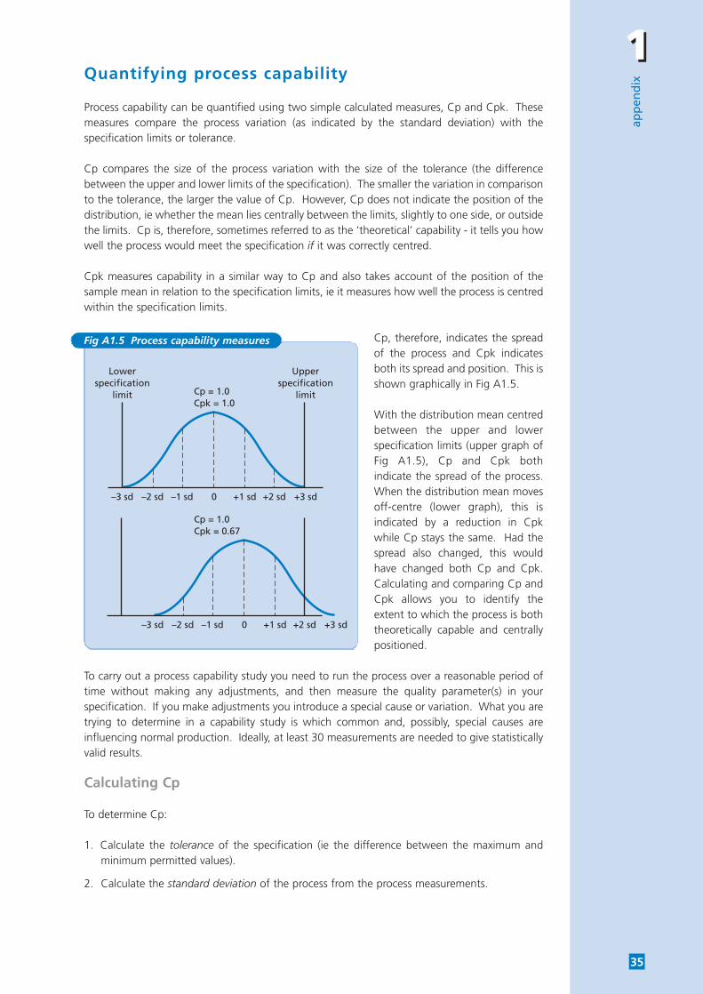
Cp, therefore, indicates the spreadof the process and Cpk indicatesboth its spread and position. This isshown graphically in Fig A1.5.

With the distribution mean centredbetween the upper and lowerspecification limits (upper graph ofFig A1.5), Cp and Cpk bothindicate the spread of the process.When the distribution mean movesoff-centre (lower graph), this isindicated by a reduction in Cpkwhile Cp stays the same. Had thespread also changed, this wouldhave changed both Cp and Cpk.Calculating and comparing Cp andCpk allows you to identify theextent to which the process is boththeoretically capable and centrallypositioned.

To carry out a process capability study you need to run the process over a reasonable period oftime without making any adjustments, and then measure the quality parameter(s) in yourspecification. If you make adjustments you introduce a special cause or variation. What you aretrying to determine in a capability study is which common and, possibly, special causes areinfluencing normal production. Ideally, at least 30 measurements are needed to give statisticallyvalid results.

Calculating Cp

To determine Cp:

1. Calculate the tolerance of the specification (ie the difference between the maximum andminimum permitted values).

2. Calculate the standard deviation of the process from the process measurements.

–1 sd +1 sd +2 sd +3 sd–2 sd–3 sd 0

Lowerspecification

limit

Upperspecification

limitCp = 1.0Cpk = 1.0

–1 sd +1 sd +2 sd +3 sd–2 sd–3 sd 0

Cp = 1.0Cpk = 0.67

Fig A1.5 Process capability measures

11ap

pen

dix

36

3. Divide the tolerance by six times the standard deviation of the process, ie

Cp = specification toleranceStandard deviation × 6

A Cp of 1.0 means that the process is theoretically ‘capable’, ie the tolerance of the specificationequals six times the process standard deviation.

If the process is correctly centred (ie it has been set up so that the mean value of the processequals the centre of the specification), the tolerance limits (the maximum and minimumpermitted values) will be located at ± three times the standard deviation on the process’s normaldistribution curve (see Fig A1.5).

The number of measurements within ± three standard deviations of the mean on a normaldistribution curve is 99.7%, with only 0.3% (three measurements in 1 000 or 3 000 measurementsin a million) lying outside three standard deviations and, therefore, outside the tolerance limits.

In practice, real processes are not centred exactly and it is, therefore, usual to aim for a Cp valueof at least 1.3. This provides some leeway, allowing the process to drift a little off-centre whilestill maintaining low levels of out-of-specification results (companies producing components forthe motor industry are usually required to have a process with a Cp of at least 1.3, or to beworking and investing to achieve this).

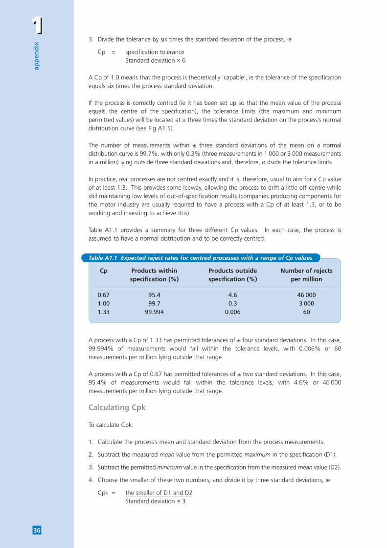
Table A1.1 provides a summary for three different Cp values. In each case, the process isassumed to have a normal distribution and to be correctly centred.

A process with a Cp of 1.33 has permitted tolerances of ± four standard deviations. In this case,99.994% of measurements would fall within the tolerance levels, with 0.006% or 60measurements per million lying outside that range.

A process with a Cp of 0.67 has permitted tolerances of ± two standard deviations. In this case,95.4% of measurements would fall within the tolerance levels, with 4.6% or 46 000measurements per million lying outside that range.

Calculating Cpk

To calculate Cpk:

1. Calculate the process’s mean and standard deviation from the process measurements.

2. Subtract the measured mean value from the permitted maximum in the specification (D1).

3. Subtract the permitted minimum value in the specification from the measured mean value (D2).

4. Choose the smaller of these two numbers, and divide it by three standard deviations, ie

Cpk = the smaller of D1 and D2Standard deviation × 3

Cp Products within Products outside Number of rejects specification (%) specification (%) per million

0.67 95.4 4.6 46 0001.00 99.7 0.3 3 0001.33 99.994 0.006 60

Table A1.1 Expected reject rates for centred processes with a range of Cp values

11

app

end

ix

37

In the case of industrial measurements, the Cpk value will usually be smaller than the Cp value,reflecting the effect of poor centring. As in the case of Cp values, a Cpk of 1.3 or above isusually taken as a sign that a process is performing well with some leeway for drift.

A decreasing Cpk value is a good indicator that special causes of variation are creeping in, egchanges in process equipment or materials.

One of the purposes of statistical process control charts (see Section 8 and Appendix 2) is todetect this happening.

22ap

pen

dix

38

Process control charts

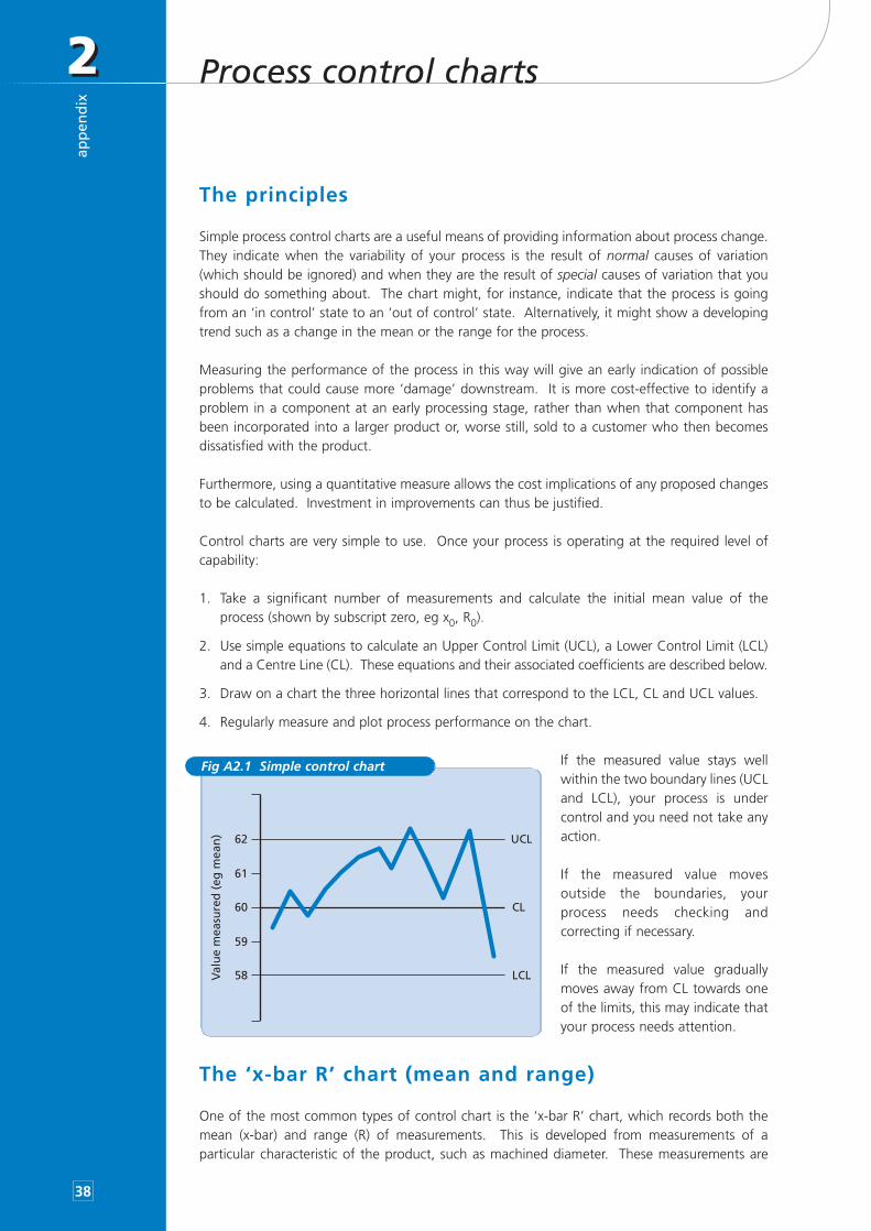
The principles

Simple process control charts are a useful means of providing information about process change.They indicate when the variability of your process is the result of normal causes of variation(which should be ignored) and when they are the result of special causes of variation that youshould do something about. The chart might, for instance, indicate that the process is goingfrom an ‘in control’ state to an ‘out of control’ state. Alternatively, it might show a developingtrend such as a change in the mean or the range for the process.

Measuring the performance of the process in this way will give an early indication of possibleproblems that could cause more ‘damage’ downstream. It is more cost-effective to identify aproblem in a component at an early processing stage, rather than when that component hasbeen incorporated into a larger product or, worse still, sold to a customer who then becomesdissatisfied with the product.

Furthermore, using a quantitative measure allows the cost implications of any proposed changesto be calculated. Investment in improvements can thus be justified.

Control charts are very simple to use. Once your process is operating at the required level ofcapability:

1. Take a significant number of measurements and calculate the initial mean value of theprocess (shown by subscript zero, eg x0, R0).

2. Use simple equations to calculate an Upper Control Limit (UCL), a Lower Control Limit (LCL)and a Centre Line (CL). These equations and their associated coefficients are described below.

3. Draw on a chart the three horizontal lines that correspond to the LCL, CL and UCL values.

4. Regularly measure and plot process performance on the chart.

If the measured value stays wellwithin the two boundary lines (UCLand LCL), your process is undercontrol and you need not take anyaction.

If the measured value movesoutside the boundaries, yourprocess needs checking andcorrecting if necessary.

If the measured value graduallymoves away from CL towards oneof the limits, this may indicate thatyour process needs attention.

The ‘x-bar R’ chart (mean and range)

One of the most common types of control chart is the ‘x-bar R’ chart, which records both themean (x-bar) and range (R) of measurements. This is developed from measurements of aparticular characteristic of the product, such as machined diameter. These measurements are

UCL

LCL

CL

62

61

60

59

58Val

ue

mea

sure

d (

eg m

ean

)

Fig A2.1 Simple control chart

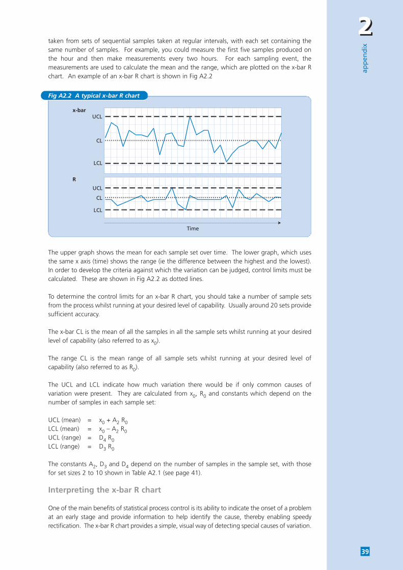
22

app

end

ix

39

taken from sets of sequential samples taken at regular intervals, with each set containing thesame number of samples. For example, you could measure the first five samples produced onthe hour and then make measurements every two hours. For each sampling event, themeasurements are used to calculate the mean and the range, which are plotted on the x-bar Rchart. An example of an x-bar R chart is shown in Fig A2.2

The upper graph shows the mean for each sample set over time. The lower graph, which usesthe same x axis (time) shows the range (ie the difference between the highest and the lowest).In order to develop the criteria against which the variation can be judged, control limits must becalculated. These are shown in Fig A2.2 as dotted lines.

To determine the control limits for an x-bar R chart, you should take a number of sample setsfrom the process whilst running at your desired level of capability. Usually around 20 sets providesufficient accuracy.

The x-bar CL is the mean of all the samples in all the sample sets whilst running at your desiredlevel of capability (also referred to as x0).

The range CL is the mean range of all sample sets whilst running at your desired level ofcapability (also referred to as R0).

The UCL and LCL indicate how much variation there would be if only common causes ofvariation were present. They are calculated from x0, R0 and constants which depend on thenumber of samples in each sample set:

UCL (mean) = x0 + A2 R0LCL (mean) = x0 – A2 R0UCL (range) = D4 R0LCL (range) = D3 R0

The constants A2, D3 and D4 depend on the number of samples in the sample set, with thosefor set sizes 2 to 10 shown in Table A2.1 (see page 41).

Interpreting the x-bar R chart

One of the main benefits of statistical process control is its ability to indicate the onset of a problemat an early stage and provide information to help identify the cause, thereby enabling speedyrectification. The x-bar R chart provides a simple, visual way of detecting special causes of variation.

Time

UCL

CL

CL

LCL

LCL

UCL

x-bar

R

Fig A2.2 A typical x-bar R chart

22ap

pen

dix

40

If only common causes of variation are present, the sample set ‘means and ranges’ willconcentrate around the CL and thin-out towards the UCL and the LCL. In fact, if the process hasa normal distribution curve, only 0.3% of the points would be expected to cross the UCL andLCL. The presence of one or more points beyond either control limit strongly indicates an out-of-control situation, and the presence of a special cause of variation.

Furthermore, when under control, the distribution of the means and ranges each side of the CLwould be random; there would be no discernible trend. If the chart does show a trend, even ifall points are within the control limits, there is probably a special cause of variation present. Youcan apply rules to these to help identify whether a trend really exists, and many computer-basedprograms can automatically highlight any such instances for you. A commonly used rule is thatseven consecutive points falling on the same side of the CL indicates a trend caused by a specialcause. Another rule is that two out of three consecutive points greater than 0.67 of thedifference between the CL and either control limit, indicates a special cause.

When the existence of a special cause is indicated, use the control chart to help identify it asfollows:

■ Identify the likely start time of the cause by looking for the start of the trend.

■ Compare the likely start time with activities on the production line (batch changes, shiftchanges, maintenance work etc).

■ Compare the x-bar and range halves of the chart to identify whether it is just the mean whichhas moved (a potential calibration error on the equipment or material) or whether the rangehas increased as well. If needed, a repeat check of Cp and Cpk will give a more accurateindication of this.

■ Compare the chart information with that of charts on other lines in the same area, or thoserecording general variables (eg temperature).

Sample size and coefficients

While larger samples will always provide a more accurate analysis and a more rapid feedback forprocess control purposes, there are usually practical limits on the number of measurements thatyou can sensibly take for each production sample. These limits are determined by the time andcost involved.

The one-off initial investigations into variability discussed earlier in this Guide used samples ofmore than 30 measurements. This is not usually practical where routine measurements are beingtaken for process control purposes. In practice, industrial companies with processes operatingin control at a reasonable level of capability can take samples with as few as two measurements.They rarely justify samples of more than ten measurements. However, there are exceptions,notably in industries that use natural (and thus highly variable) raw materials.

Despite the small number of samples usually taken, statistical process control can be usedsuccessfully even in areas such as leather-making, biscuit production, pizza manufacture etc.There are two important points to remember:

■ Where samples are very small, it is not usually worth calculating the standard deviation.Common practice is, therefore, to calculate the range (maximum – minimum values) and toconvert this to a notional standard deviation value using constants such as those shown inTable A2.1.

■ The rule of thumb when dealing with small numbers of discrete events (eg product rejects) isto do nothing until certain.

22

app

end

ix

41

Coefficients

Control chart limits should really be based on the standard deviation of the characteristic beingmeasured. However, as indicated previously, range is often used as a much more convenientmeasure of variability, especially with low sample size. Table A2.1 shows constants derived bystatisticians for the calculation of control limits from range values. Sample sizes are from two to ten.

Types of process control chart

There are several types of process control chart, each plotting slightly different variables and eachusing different statistical rules to calculate the LCL, CL and UCL values. They take into accountfactors such as skewness in a distribution and the effects of sample size.

You can easily select the type of chart you need to use by looking at the headings in each case.You do not need to understand details of the statistical theory underlying the different types.

Charts used where product properties involve fractional values

Two types of chart are used where the parameters measured are continuous - length, weight,concentration etc: the x-bar R chart and the moving average and range chart.

n A2 D3 D4

2 1.880 * 3.2673 1.023 * 2.5754 0.729 * 2.2825 0.577 * 2.1156 0.483 * 2.0047 0.419 0.076 1.9248 0.373 0.136 1.8649 0.337 0.184 1.81610 0.308 0.223 1.777

* The value of D3 is not considered for a sample of <7, and the lower limit for the range is effectively zero.

Table A2.1 Control chart coefficients for values of n of up to 10

Used where several measurements (ie several values of x) are taken at each samplingtime.

The chart has two components:

■ the x-bar component, which plots the average value of each sample of nmeasurements (ie all the measurements taken at any one time);

■ the R component, which plots the range of the sample (maximum value –minimum value).

Control limits for x-bar chart Control limits for R chart

UCL = x0 + A2 R0 UCL = D4 R0CL = x0 CL = R0LCL = x0 – A2 R0 LCL = D3 R0

where x0 and R0 are mean values of the process and where A2, D3 and D4 arecoefficients associated with each value of n (see Table A2.1).

x-bar R chart

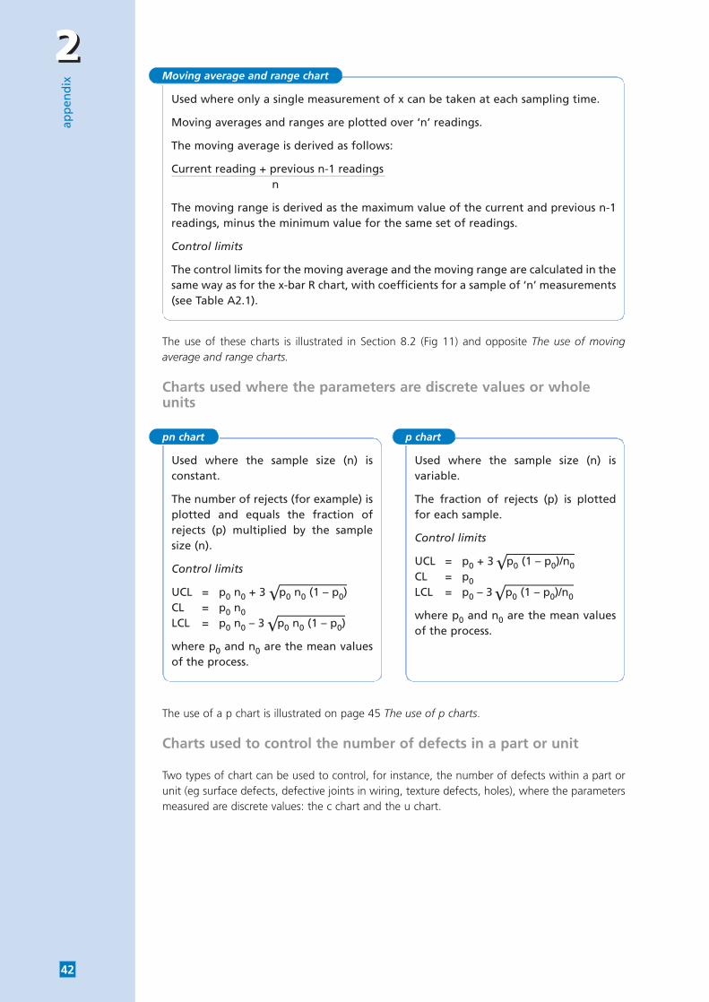
22ap

pen

dix

42

The use of these charts is illustrated in Section 8.2 (Fig 11) and opposite The use of movingaverage and range charts.

Charts used where the parameters are discrete values or wholeunits

The use of a p chart is illustrated on page 45 The use of p charts.

Charts used to control the number of defects in a part or unit

Two types of chart can be used to control, for instance, the number of defects within a part orunit (eg surface defects, defective joints in wiring, texture defects, holes), where the parametersmeasured are discrete values: the c chart and the u chart.

Used where only a single measurement of x can be taken at each sampling time.

Moving averages and ranges are plotted over ‘n’ readings.

The moving average is derived as follows:

Current reading + previous n-1 readingsn

The moving range is derived as the maximum value of the current and previous n-1readings, minus the minimum value for the same set of readings.

Control limits

The control limits for the moving average and the moving range are calculated in thesame way as for the x-bar R chart, with coefficients for a sample of ‘n’ measurements(see Table A2.1).

Moving average and range chart

Used where the sample size (n) isconstant.

The number of rejects (for example) isplotted and equals the fraction ofrejects (p) multiplied by the samplesize (n).

Control limits

UCL = p0 n0 + 3 p0 n0 (1 – p0)CL = p0 n0LCL = p0 n0 – 3 p0 n0 (1 – p0)

where p0 and n0 are the mean valuesof the process.

pn chart

Used where the sample size (n) isvariable.

The fraction of rejects (p) is plottedfor each sample.

Control limits

UCL = p0 + 3 p0 (1 – p0)/n0CL = p0LCL = p0 – 3 p0 (1 – p0)/n0

where p0 and n0 are the mean valuesof the process.

p chart

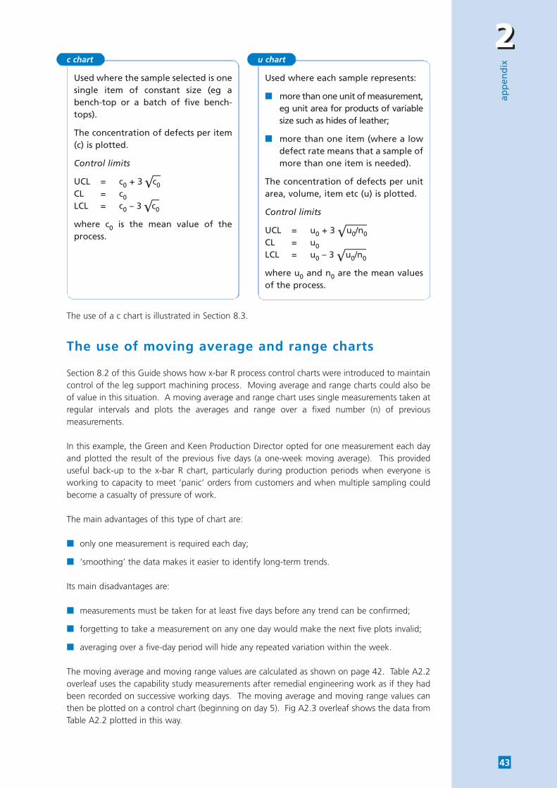
22

app

end

ix

43

The use of a c chart is illustrated in Section 8.3.

The use of moving average and range charts

Section 8.2 of this Guide shows how x-bar R process control charts were introduced to maintaincontrol of the leg support machining process. Moving average and range charts could also beof value in this situation. A moving average and range chart uses single measurements taken atregular intervals and plots the averages and range over a fixed number (n) of previousmeasurements.

In this example, the Green and Keen Production Director opted for one measurement each dayand plotted the result of the previous five days (a one-week moving average). This provideduseful back-up to the x-bar R chart, particularly during production periods when everyone isworking to capacity to meet ‘panic’ orders from customers and when multiple sampling couldbecome a casualty of pressure of work.

The main advantages of this type of chart are:

■ only one measurement is required each day;

■ ‘smoothing’ the data makes it easier to identify long-term trends.

Its main disadvantages are:

■ measurements must be taken for at least five days before any trend can be confirmed;

■ forgetting to take a measurement on any one day would make the next five plots invalid;

■ averaging over a five-day period will hide any repeated variation within the week.

The moving average and moving range values are calculated as shown on page 42. Table A2.2overleaf uses the capability study measurements after remedial engineering work as if they hadbeen recorded on successive working days. The moving average and moving range values canthen be plotted on a control chart (beginning on day 5). Fig A2.3 overleaf shows the data fromTable A2.2 plotted in this way.

Used where the sample selected is onesingle item of constant size (eg a bench-top or a batch of five bench-tops).

The concentration of defects per item(c) is plotted.

Control limits

UCL = c0 + 3 c0CL = c0LCL = c0 – 3 c0

where c0 is the mean value of theprocess.

c chart

Used where each sample represents:

■ more than one unit of measurement,eg unit area for products of variablesize such as hides of leather;

■ more than one item (where a lowdefect rate means that a sample ofmore than one item is needed).

The concentration of defects per unitarea, volume, item etc (u) is plotted.

Control limits

UCL = u0 + 3 u0/n0CL = u0LCL = u0 – 3 u0/n0

where u0 and n0 are the mean valuesof the process.

u chart

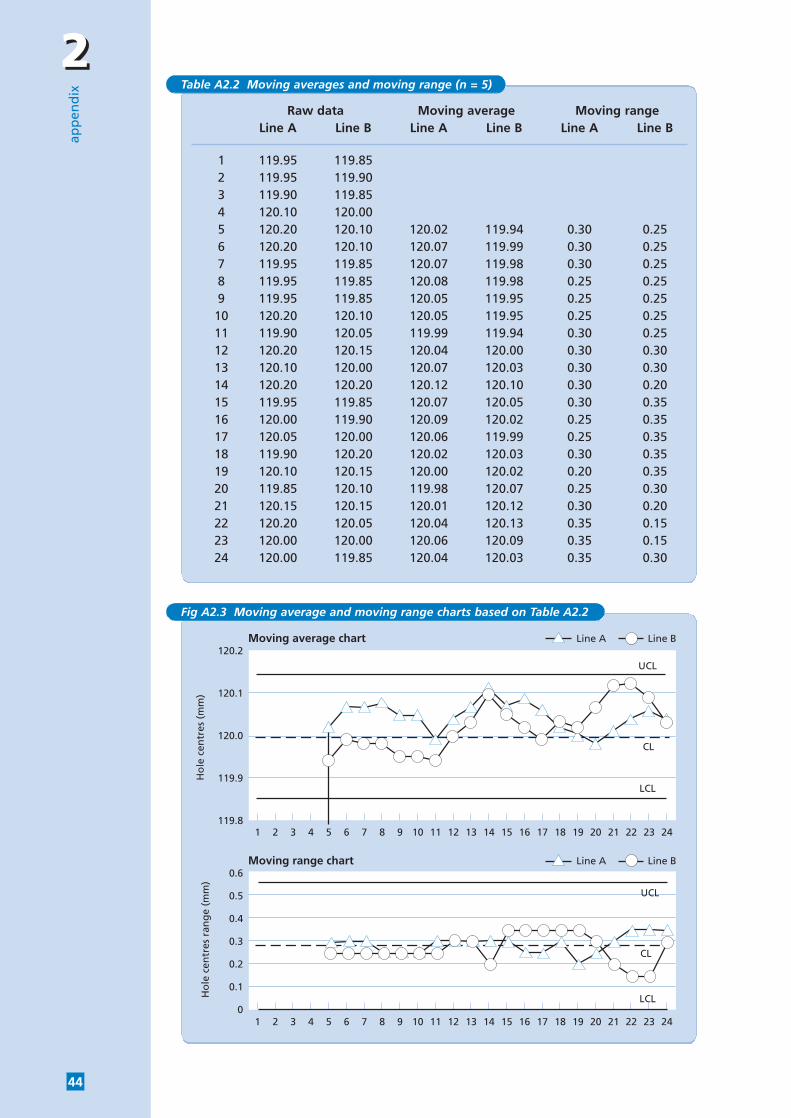
22ap

pen

dix

44

Raw data Moving average Moving rangeLine A Line B Line A Line B Line A Line B

1 119.95 119.852 119.95 119.903 119.90 119.854 120.10 120.005 120.20 120.10 120.02 119.94 0.30 0.256 120.20 120.10 120.07 119.99 0.30 0.257 119.95 119.85 120.07 119.98 0.30 0.258 119.95 119.85 120.08 119.98 0.25 0.259 119.95 119.85 120.05 119.95 0.25 0.25

10 120.20 120.10 120.05 119.95 0.25 0.2511 119.90 120.05 119.99 119.94 0.30 0.2512 120.20 120.15 120.04 120.00 0.30 0.3013 120.10 120.00 120.07 120.03 0.30 0.3014 120.20 120.20 120.12 120.10 0.30 0.2015 119.95 119.85 120.07 120.05 0.30 0.3516 120.00 119.90 120.09 120.02 0.25 0.3517 120.05 120.00 120.06 119.99 0.25 0.3518 119.90 120.20 120.02 120.03 0.30 0.3519 120.10 120.15 120.00 120.02 0.20 0.3520 119.85 120.10 119.98 120.07 0.25 0.3021 120.15 120.15 120.01 120.12 0.30 0.2022 120.20 120.05 120.04 120.13 0.35 0.1523 120.00 120.00 120.06 120.09 0.35 0.1524 120.00 119.85 120.04 120.03 0.35 0.30

Table A2.2 Moving averages and moving range (n = 5)

UCL

CL

LCL

LCL

Line A Line B120.2

120.1

120.0

119.9

119.8

Ho

le c

entr

es (

mm

)

Moving average chart

1 2 3 4 5 6 7 8 9 10 11 12 13 14 15 16 17 18 19 20 21 22 23 24

UCL

CL

Line A Line B0.6

0.5

0.4

0.3

0.2

0.1

0

Ho

le c

entr

es r

ang

e (m

m)

Moving range chart

1 2 3 4 5 6 7 8 9 10 11 12 13 14 15 16 17 18 19 20 21 22 23 24

Fig A2.3 Moving average and moving range charts based on Table A2.2

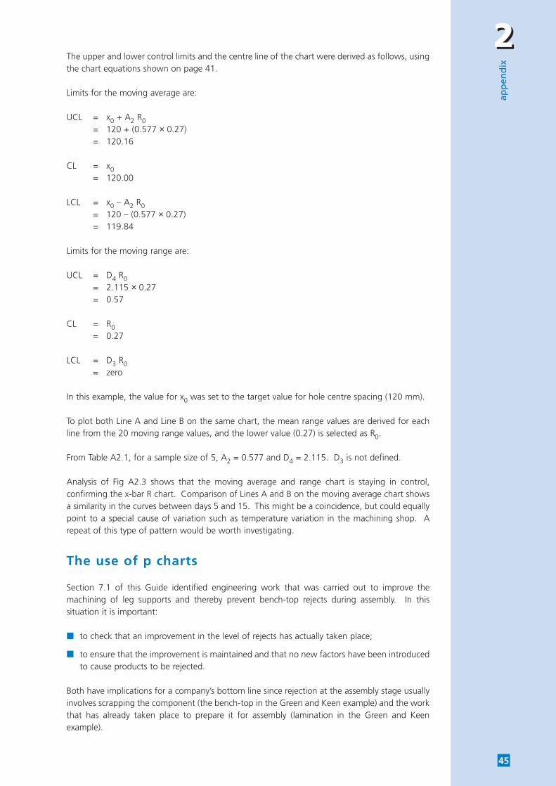
22

app

end

ix

45

The upper and lower control limits and the centre line of the chart were derived as follows, usingthe chart equations shown on page 41.

Limits for the moving average are:

UCL = x0 + A2 R0= 120 + (0.577 × 0.27)= 120.16

CL = x0= 120.00

LCL = x0 – A2 R0= 120 – (0.577 × 0.27)= 119.84

Limits for the moving range are:

UCL = D4 R0= 2.115 × 0.27= 0.57

CL = R0= 0.27

LCL = D3 R0= zero

In this example, the value for x0 was set to the target value for hole centre spacing (120 mm).

To plot both Line A and Line B on the same chart, the mean range values are derived for eachline from the 20 moving range values, and the lower value (0.27) is selected as R0.

From Table A2.1, for a sample size of 5, A2 = 0.577 and D4 = 2.115. D3 is not defined.

Analysis of Fig A2.3 shows that the moving average and range chart is staying in control,confirming the x-bar R chart. Comparison of Lines A and B on the moving average chart showsa similarity in the curves between days 5 and 15. This might be a coincidence, but could equallypoint to a special cause of variation such as temperature variation in the machining shop. Arepeat of this type of pattern would be worth investigating.

The use of p charts

Section 7.1 of this Guide identified engineering work that was carried out to improve themachining of leg supports and thereby prevent bench-top rejects during assembly. In thissituation it is important:

■ to check that an improvement in the level of rejects has actually taken place;

■ to ensure that the improvement is maintained and that no new factors have been introducedto cause products to be rejected.

Both have implications for a company’s bottom line since rejection at the assembly stage usuallyinvolves scrapping the component (the bench-top in the Green and Keen example) and the workthat has already taken place to prepare it for assembly (lamination in the Green and Keenexample).

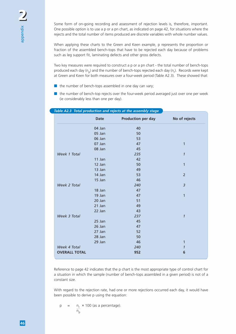
22ap

pen

dix

46

Some form of on-going recording and assessment of rejection levels is, therefore, important.One possible option is to use a p or a pn chart, as indicated on page 42, for situations where therejects and the total number of items produced are discrete variables with whole number values.

When applying these charts to the Green and Keen example, p represents the proportion orfraction of the assembled bench-tops that have to be rejected each day because of problemssuch as leg support fit, laminating defects and other gross defects.

Two key measures were required to construct a p or a pn chart - the total number of bench-topsproduced each day (np) and the number of bench-tops rejected each day (nr). Records were keptat Green and Keen for both measures over a four-week period (Table A2.3). These showed that:

■ the number of bench-tops assembled in one day can vary;

■ the number of bench-top rejects over the four-week period averaged just over one per week(ie considerably less than one per day).

Reference to page 42 indicates that the p chart is the most appropriate type of control chart fora situation in which the sample (number of bench-tops assembled in a given period) is not of aconstant size.

With regard to the rejection rate, had one or more rejections occurred each day, it would havebeen possible to derive p using the equation:

p = nr × 100 (as a percentage).np

Date Production per day No of rejects

04 Jan 4005 Jan 5006 Jan 5307 Jan 47 108 Jan 45

Week 1 Total 235 111 Jan 4212 Jan 50 113 Jan 4914 Jan 53 215 Jan 46

Week 2 Total 240 318 Jan 4719 Jan 47 120 Jan 5121 Jan 4922 Jan 43

Week 3 Total 237 125 Jan 4526 Jan 4727 Jan 5228 Jan 5029 Jan 46 1

Week 4 Total 240 1OVERALL TOTAL 952 6

Table A2.3 Total production and rejects at the assembly stage

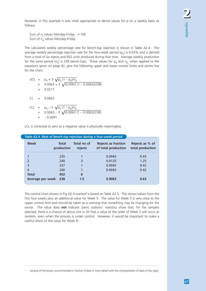
22

app

end

ix

47

However, in this example it was more appropriate to derive values for p on a weekly basis asfollows:

Sum of nr values Monday-Friday × 100Sum of np values Monday-Friday

The calculated weekly percentage rate for bench-top rejection is shown in Table A2.4. Theaverage weekly percentage rejection rate for the four-week period (p0) is 0.63% and is derivedfrom a total of six rejects and 952 units produced during that time. Average weekly productionfor the same period (n0) is 238 bench-tops. These values for p0 and n0, when applied to theequations given on page 42, give the following upper and lower control limits and centre linefor the chart:

UCL = p0 + 3 p0 (1 – p0)/n0

= 0.0063 + 3 (0.0063 (1 – 0.0063)/238)

= 0.0217

CL = 0.0063

LCL = p0 – 3 p0 (1 – p0)/n0

= 0.0063 – 3 (0.0063 (1 – 0.0063)/238)

= – 0.0091

LCL is corrected to zero as a negative value is physically meaningless.

The control chart shown in Fig A2.4 overleaf is based on Table A2.5. This shows values from thefirst four weeks plus an additional value for Week 5. The value for Week 5 is very close to theupper control limit and should be taken as a warning that something may be changing for theworse. The value does not indicate ‘panic stations’: statistics show that, for the samplesselected, there is a chance of about one in 20 that a value of the order of Week 5 will occur atrandom, even when the process is under control. However, it would be important to make acareful check of the value for Week 62.

2 Several of the books recommended in Section 9 deal in more detail with the interpretation of data of this type.

Week Total Total no of Rejects as fraction Rejects as % of production rejects of total production total production

1 235 1 0.0043 0.432 240 3 0.0125 1.253 237 1 0.0042 0.424 240 1 0.0042 0.42Total 952 6Average per week 238 1.5 0.0063 0.63

Table A2.4 Rate of bench-top rejection during a four-week period

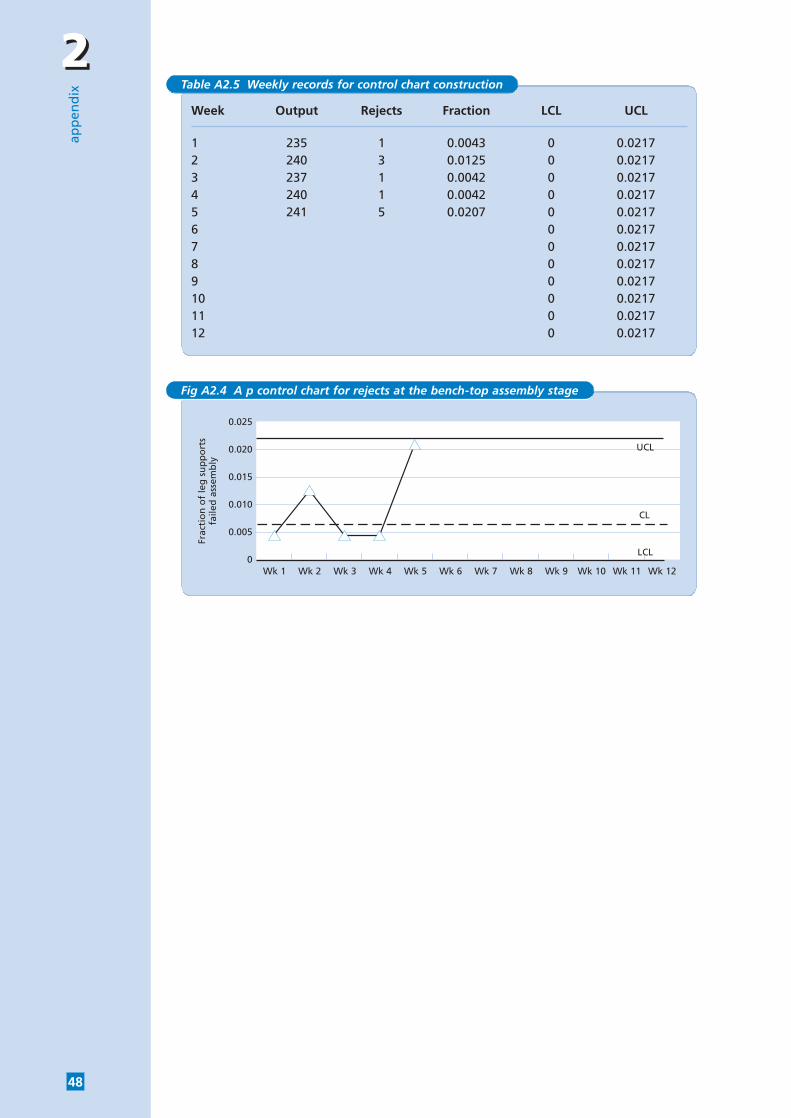
22ap

pen

dix

48

Week Output Rejects Fraction LCL UCL

1 235 1 0.0043 0 0.02172 240 3 0.0125 0 0.02173 237 1 0.0042 0 0.02174 240 1 0.0042 0 0.02175 241 5 0.0207 0 0.02176 0 0.02177 0 0.02178 0 0.02179 0 0.021710 0 0.021711 0 0.021712 0 0.0217

Table A2.5 Weekly records for control chart construction

UCL

CL

LCL

0.025

0.020

0.015

0.010

0.005

0

Frac

tio

n o

f le

g s

up

po

rts

faile

d a

ssem

bly

Wk 1 Wk 2 Wk 3 Wk 4 Wk 5 Wk 6 Wk 7 Wk 8 Wk 9 Wk 10 Wk 11 Wk 12

Fig A2.4 A p control chart for rejects at the bench-top assembly stage

For further informationplease contact the

Environmentand EnergyHelpline0800 585794

Envirowise – Practical Environmental Advice for Business – is a Government programmethat offers free, independent and practical advice to UK businesses to reduce waste atsource and increase profits. It is managed by AEA Technology Environment and NPLManagement Limited.

Envirowise offers a range of free services including:

Free advice from Envirowise experts through the Environment and EnergyHelpline.

A variety of publications that provide up-to-date information on wasteminimisation issues, methods and successes.

Free, on-site waste reviews from Envirowise consultants, called Fast Track Visits,that help businesses identify and realise savings.

Guidance on Waste Minimisation Clubs across the UK that provide a chance forlocal companies to meet regularly and share best practices in waste minimisation.

Best practice seminars and practical workshops that offer an ideal way toexamine waste minimisation issues and discuss opportunities and methodologies.

© Crown copyright. First printed February 2001. Printed on paper containing a minimum of 75% post-consumer waste.This material may be freely reproduced in its original form except for sale or advertising purposes.

Harwell International Business Centre | 156 Curie Avenue | Didcot | Oxfordshire | OX11 0QJE-mail: [email protected] Internet: www.envirowise.gov.uk

Practical Environmental Advice for Business

preventing waste in production: practical methods for ...infohouse.p2ric.org/ref/24/23122.pdf ·...

Documents