pressure vessel design - download.e-bookshelf.de · speciﬁcally, pressure vessels represent...

Pressure Vessel Design

123

Donatello Annaratone

Pressure Vessel Design

With 275 Figures and 4 Tables

Library of Congress Control Number:

This work is subject to copyright. All rights are reserved, whether the whole or part of the materialis concerned, specifically the rights of translation, reprinting, reuse of illustrations, recitation, broad-casting, reproduction on microfilm or in any other way, and storage in data banks. Duplication ofthis publication or parts thereof is permitted only under the provisions of the German Copyright Law

Springer. Violations are liable to prosecution under the German Copyright Law.

Springer is a part of Springer Science+Business Media.

springer.com

The use of general descriptive names, registered names, trademarks, etc. in this publication does notimply, even in the absence of a specific statement, that such names are exempt from the relevant pro-tective laws and regulations and therefore free for general use.

Printed on acid-free paper 5 4 3 2 1 0

macro packageA ELT X

62/3100/SPi

© Springer-Verlag Berlin Heidelberg 2007

Donatello AnnaratoneVia Ceradini 1420129 MilanoItaly

2006936077

ISBN-10 3-540-49142-2 Springer Berlin Heidelberg New York

of September 9, 1965, in its current version, and permission for use must always be obtained from

ISBN-13 978-3-540-49142-2 Springer Berlin Heidelberg New York

Typesetting by author and SPi using a Springer

SPIN 11607205

e-mail: [email protected]

Cover design: eStudio Calamar, Girona, Spain.

Preface

1 Industrial Sectors Interested in Pressure Vessels

Pressure vessels are probably the most widespread “machines” within thedifferent industrial sectors. In fact, there is no factory without pressure vessels,steam boilers, tanks, autoclaves, collectors, heat exchangers, pipes, etc. Morespecifically, pressure vessels represent fundamental components in sectors ofenormous industrial importance, such as the nuclear, oil, petrochemical, andchemical sectors. There are periodic international symposia on the problemsrelated to the verification of pressure vessels.

For many years an ISO committee was dedicated to pressure vessels design.There is also a technical committee of the EU specifically assigned to thisfield. All the industrialized countries have a code relative to pressure vesselsdesign. However, even when the code includes specific regulations to determinethe thickness of the different components, typically not all issues facing thedesigner are discussed. Finally, it is worth noting that a few regulations causesome perplexity.

In Italy, a specific area of ISPESL regulations (VSR collection) is devotedto pressure vessels.

2 Current Know-How with Regard to ResistanceVerification

A pressure vessel is not an easy machinery in terms of resistance verification.A layman can easily make the mistake of considering somewhat simple struc-tural forms that are in fact quite difficult to analyze, especially if one would liketo apply the most modern criteria of verification (elastoplasticity, self-limitingstresses, etc.).

Regardless of the enormous interest in the topic and numerous efforts,many problems have not been studied in-depth, and there is still no agree-ment among scholars and the institutions of the various countries that define

VI Preface

regulations. In addition, economical reasons and technical progress constantlypresent new challenges in connection with new forms and solutions, thenecessity to reduce thickness to a minimum, etc.

Finally, the growth of the nuclear sector has highlighted the necessity ofan investigation beyond the simplistic analysis of stresses, and this also ledto a systematic analysis of the impact of fatigue phenomena. These accom-plishments notwithstanding, much still needs to be done if, from a practicalstandpoint, one wishes to move from general principles to operational guide-lines of calculation criteria that are as simple as possible.

3 Current State of Technical Literature

With regard to Italy, when pressure vessels are treated, they are included ingeneral textbooks about mechanical engineering. This leads to a somewhatgeneric and often outdated treatment of the subject with regard to modernverification criteria, and hence the outcome is of little practical interest.Outside of Italy, there are textbooks and various publications specifically onpressure vessels.

However, these publications have a number of shortcomings:

(a) Simply a guide to apply the code’s rules correctly.(b) Sound scholarly framework that often does not extend itself to the point

of analyzing the practical cases, thus becoming of little use to the designer.(c) Lack of interest in problems that may seem marginal but are in reality

those causing many obstacles to the designer, specifically those that arenot analyzed in detail and also happen not to be included in regulationsand codes.

(d) Experimental emphasis that for the cases under study is of obvious help.However, because the number of cases is considerable, and a theoreticalbackground is lacking, the designer is unable to use the available data byapplying “similarity approaches.”

(e) Lack of interest in verification methodology which is essential for sizing;the designer is faced with values for stresses that he or she does notknow how to evaluate; the situation becomes even more complex whenthe verification methodology exists but does not correspond to the modernverification criteria.

4 General Characteristics of the Book

The book focuses on general problems as well as fundamental ones derivedfrom the previous ones, and on problems that may be incorrectly consideredof secondary importance but are in fact crucial in the design phase.

The basic approach is rigorously scientific with a complete theoreticaldevelopment of the topics treated, but the analysis is always pushed so far as to

Preface VII

offer concrete and precise calculation criteria that can be immediately appliedto actual designs. This is accomplished through appropriate algorithms thatlead to final equations or to characteristic parameters defined through math-ematical equations. Given the complexity of many of these, representativegraphs are shown.

In other cases experimental graphs are shown. Their limit of applicabilityis discussed, also by including a basic theoretical treatment to justify theirspecific behavior. The result of this is a textbook with a large number ofequations and graphs, both fundamental for the actual design of pressurevessels.

The topics treated are grouped in ten chapters.The first chapter describes how to achieve verification criteria, the second

analyzes a few general problems, such as stresses of the membrane in revo-lution solids and edge effects. The third chapter deals with cylinders underpressure from the inside, while the fourth focuses on cylinders under pressurefrom the outside. The fifth chapter covers spheres, and the sixth is about alltypes of heads. Chapter seven discusses different components of particularshape as well as pipes, with special attention to flanges. The eighth chapterdiscusses the influence of holes, while the ninth is devoted to the influence ofsupports. Finally, chapter ten illustrates the fundamental criteria regardingfatigue analysis.

5 Original Contributions of the Author to the Solutionof Various Problems

Besides the rather unique approach to the entire work, see Sect. 4 above, originalcontributions can be found in most chapters, thanks to the author’s numerouspublications on the topic and to studies performed ad hoc for this book.

Specifically, we would like to draw your attention to the following topics:

3.4 Allowable out of Roundness3.5 Stiffened Cylinders3.6 Partially Plastic Deformed Cylinders3.7 Stresses due to Thickness Variation4.2 and 4.3 Cylinders Under External Pressure (special emphasis on

ovalization)5.4 Partially Plastic Deformed Spheres6.4 Flat Heads7.4 Flanges7.6 Expansion Compensators8.3 Isolated Holes on Cylinders, Spheres, and Cones: Y and T Branches8.4 Flat Head with Central Hole8.5 Drilled Plates9.2 Spherical Vessels Resting on a Parallel

Contents

1 Preliminary Considerations . . . . . . . . . . . . . . . . . . . . . . . . . . . . . . . . 11.1 Mechanical Characteristics of Steel . . . . . . . . . . . . . . . . . . . . . . . . 11.2 Allowable Stress . . . . . . . . . . . . . . . . . . . . . . . . . . . . . . . . . . . . . . . . . 71.3 Theories of Failure . . . . . . . . . . . . . . . . . . . . . . . . . . . . . . . . . . . . . . . 91.4 Plasticity Collaboration . . . . . . . . . . . . . . . . . . . . . . . . . . . . . . . . . . 131.5 Verification Criteria . . . . . . . . . . . . . . . . . . . . . . . . . . . . . . . . . . . . . . 18

1.5.1 General Membrane Stresses (σm) . . . . . . . . . . . . . . . . . . . . 191.5.2 Local Membrane Stresses (σml) . . . . . . . . . . . . . . . . . . . . . 191.5.3 Primary Bending Stresses (σf ) . . . . . . . . . . . . . . . . . . . . . . 191.5.4 Secondary Stresses (σsec) . . . . . . . . . . . . . . . . . . . . . . . . . . . 201.5.5 Peak Stresses (σpic) . . . . . . . . . . . . . . . . . . . . . . . . . . . . . . . . 21

2 General Calculation Criteria . . . . . . . . . . . . . . . . . . . . . . . . . . . . . . . 232.1 Membrane Stresses in Revolution Shells . . . . . . . . . . . . . . . . . . . . 232.2 Edge Effects in Cylinders and Semispheres . . . . . . . . . . . . . . . . . . 262.3 Stress Concentration Around Holes . . . . . . . . . . . . . . . . . . . . . . . . 36

3 Cylinders Under Internal Pressure . . . . . . . . . . . . . . . . . . . . . . . . . 473.1 General Design Criteria . . . . . . . . . . . . . . . . . . . . . . . . . . . . . . . . . . 473.2 Thick Cylinders . . . . . . . . . . . . . . . . . . . . . . . . . . . . . . . . . . . . . . . . . 613.3 Thermal Stresses . . . . . . . . . . . . . . . . . . . . . . . . . . . . . . . . . . . . . . . . 633.4 Allowable Out of Roundness . . . . . . . . . . . . . . . . . . . . . . . . . . . . . . 773.5 Two-Wall, Multilayer, and Stiffened Cylinders . . . . . . . . . . . . . . . 813.6 Partially Plastic Deformed Cylinders . . . . . . . . . . . . . . . . . . . . . . . 1003.7 Stresses Due to Thickness Variation . . . . . . . . . . . . . . . . . . . . . . . . 109

4 Cylinders Under External Pressure . . . . . . . . . . . . . . . . . . . . . . . . 1274.1 Thick Cylinders . . . . . . . . . . . . . . . . . . . . . . . . . . . . . . . . . . . . . . . . . 1274.2 Thin Cylinders of Infinite Length . . . . . . . . . . . . . . . . . . . . . . . . . . 1324.3 Stiffened Cylinders . . . . . . . . . . . . . . . . . . . . . . . . . . . . . . . . . . . . . . 1394.4 Stiffening Rings . . . . . . . . . . . . . . . . . . . . . . . . . . . . . . . . . . . . . . . . . 147

X Contents

5 Spherical Vessels . . . . . . . . . . . . . . . . . . . . . . . . . . . . . . . . . . . . . . . . . . 1555.1 Spheres Under Internal Pressure . . . . . . . . . . . . . . . . . . . . . . . . . . . 1555.2 Thick Spheres . . . . . . . . . . . . . . . . . . . . . . . . . . . . . . . . . . . . . . . . . . . 1655.3 Thermal Stresses . . . . . . . . . . . . . . . . . . . . . . . . . . . . . . . . . . . . . . . . 1675.4 Partially Plastic Deformed Spheres . . . . . . . . . . . . . . . . . . . . . . . . 1755.5 Spheres Under External Pressure . . . . . . . . . . . . . . . . . . . . . . . . . . 184

6 Heads . . . . . . . . . . . . . . . . . . . . . . . . . . . . . . . . . . . . . . . . . . . . . . . . . . . . . 1896.1 Hemispherical Heads . . . . . . . . . . . . . . . . . . . . . . . . . . . . . . . . . . . . . 1896.2 Dished Heads . . . . . . . . . . . . . . . . . . . . . . . . . . . . . . . . . . . . . . . . . . . 1996.3 Conical Heads and Truncated Cones . . . . . . . . . . . . . . . . . . . . . . . 2056.4 Flat Heads . . . . . . . . . . . . . . . . . . . . . . . . . . . . . . . . . . . . . . . . . . . . . 211

7 Special Components and Tubes . . . . . . . . . . . . . . . . . . . . . . . . . . . . 2417.1 Elliptical Tubes . . . . . . . . . . . . . . . . . . . . . . . . . . . . . . . . . . . . . . . . . 2417.2 Torus and Bended Tubes . . . . . . . . . . . . . . . . . . . . . . . . . . . . . . . . . 2447.3 Quadrangular Vessels . . . . . . . . . . . . . . . . . . . . . . . . . . . . . . . . . . . . 2517.4 Flanges . . . . . . . . . . . . . . . . . . . . . . . . . . . . . . . . . . . . . . . . . . . . . . . . 2667.5 Piping with Internal Warm Fluid . . . . . . . . . . . . . . . . . . . . . . . . . . 2907.6 Expansion Compensators . . . . . . . . . . . . . . . . . . . . . . . . . . . . . . . . . 297

8 The Influence of Holes . . . . . . . . . . . . . . . . . . . . . . . . . . . . . . . . . . . . . 3138.1 Hole Lines on Cylinders, Spheres, and Cones . . . . . . . . . . . . . . . . 3138.2 High Thickness Nozzles and Equivalent Diameter . . . . . . . . . . . . 3308.3 Isolated Holes on Cylinders, Spheres, and Cones:

Y and T Branches . . . . . . . . . . . . . . . . . . . . . . . . . . . . . . . . . . . . . . . 3358.4 Flat Head with Central Hole . . . . . . . . . . . . . . . . . . . . . . . . . . . . . . 3538.5 Drilled Plates . . . . . . . . . . . . . . . . . . . . . . . . . . . . . . . . . . . . . . . . . . . 3638.6 Holes in Quadrangular Vessels . . . . . . . . . . . . . . . . . . . . . . . . . . . . 370

9 The Influence of Supports . . . . . . . . . . . . . . . . . . . . . . . . . . . . . . . . . 3799.1 Cylindrical Vessels on Saddle Supports . . . . . . . . . . . . . . . . . . . . . 3799.2 Spherical Vessels Resting on a Parallel . . . . . . . . . . . . . . . . . . . . . 3879.3 Local Effects of Forces and Moments on Cylinders . . . . . . . . . . . 3969.4 Local Effects of Forces and Moments on Spheres . . . . . . . . . . . . . 417

10 Fatigue Analysis . . . . . . . . . . . . . . . . . . . . . . . . . . . . . . . . . . . . . . . . . . . 42310.1 General Approach . . . . . . . . . . . . . . . . . . . . . . . . . . . . . . . . . . . . . . . 42310.2 Fatigue Curves . . . . . . . . . . . . . . . . . . . . . . . . . . . . . . . . . . . . . . . . . . 42510.3 Vessels not Requiring Fatigue Analysis . . . . . . . . . . . . . . . . . . . . . 42810.4 Basic Criteria for Fatigue Analysis . . . . . . . . . . . . . . . . . . . . . . . . . 431

Bibliography . . . . . . . . . . . . . . . . . . . . . . . . . . . . . . . . . . . . . . . . . . . . . . . . . . . 437

Index . . . . . . . . . . . . . . . . . . . . . . . . . . . . . . . . . . . . . . . . . . . . . . . . . . . . . . . . . . 443

Notation

A Cross-sectional areaC Form factor (heads)D, d DiameterDe, de Outside diameterDi, di Inside diameterDm, dm Average diameterE Young’s modulus; modulus of elasticityF Force, loadf Basic allowable stressfc Allowable stress for pipingfa Allowable stress for fatigueH HeightI Moment of inertiak1 . . . . . . . . . k10 Dimensionless factorsL, l Length, widthM Bending momentN Normal forcen Number of waves (buckling); number of cyclesp Pressurepc, pce, pcp Critical pressuresR, r RadiusRe, re Outside radiusRi, ri Inside radiusRm, rm Average radiuss ThicknessT Shear forcet Temperatureu OvalizationW Section modulusz Weld joint efficiency; efficiency of ligamentsα Thermal expansion coefficientδ Deviation from roundnessε Deformation (strain)

XII Notation

εid Ideal deformationλ Thermal conductivity coefficientµ Poisson’s ratioν Safety factorσ Normal stressσI , σII , σIII Principal stressesσa Longitudinal stress, axial stressσm Meridian stressσr Radial stressσt Hoop stress, circumferential stressσid Ideal stressσs Yield strengthσR Rupture stressτ Shear stressα, ϑ, ϕ, ω Angles

1

Preliminary Considerations

1.1 Mechanical Characteristics of Steel

If we exert a tensile load on a specimen made of mild carbon steel, and wetransfer on the x-axis the values of the elongation per unit of length betweenthe references (ε) (called strain) and on the y-axis the values of the stress(σ) that equals the load applied to the specimen divided by its original cross-sectional area, we obtain a diagram qualitatively similar to the one shown inFig. 1.1.

We notice that there is proportionality between stress and strain in thefirst portion of the curve, i.e., the steel follows Hooke’s law that constitutesthe basis of classic calculation in the elastic field. In fact, the steel behaves inan elastic fashion, i.e., the deformations completely disappear after removalof the load, and the specimen returns to its original shape.

The angular coefficient E of the straight portion given by the relationshipσ/ε is called modulus of elasticity, or Young’s modulus. The point on thecurve at the end of the linear section identifies a value of σ which is calledproportional limit.

Steel behaves in an elastic fashion even beyond the proportional limit,as long as another characteristic point corresponding to stress called elasticlimit is not exceeded. Note that the two points mentioned above are near, andthe second one is not easy to determine. In practice, we typically equate theproportional limit to the elastic limit.

By increasing the load applied to the specimen, we reach a point on thecurve corresponding to a stress σ, called upper yield strength, that representsthe maximum value of σ taking place at the onset of the yielding phenomenon.In fact, after reaching the upper yield strength the load decreases, and wereach a relative minimum of the curve that identifies the stress called loweryield strength.

The yielding phenomenon is characterized by large deformations (whencompared to those typical of the elasticity field) under practically constantload.

2 1 Preliminary Considerations

ε

σ

Fig. 1.1

This portion of the curve is then followed by a portion characterized byprogressive increase in stress with large deformations. This is the well-knownphenomenon of steel hardening, which persists until the stress reaches a maxi-mum value called ultimate strength. After that σ decreases (again with regardto the original cross-sectional area of the specimen), and we reach rupture.

Conversely, if we consider the actual cross-sectional area of the specimen inthe different stages, the highest value of σ is reached in correspondence withthe rupture point. In fact, substantial elongations in correspondence withyielding and hardening areas happen together with a significant reduction ofthe cross-sectional area.

The lower value of the yield strength (simply known as “yield strength,”σs) and the maximum value of σ that precedes the rupture are the mostsignificant parameters of the steel’s mechanical properties, and are thereforeindicated in test certificates and represent the basis of resistance calculus.

The yield strength basically shows the condition under which the materialstarts yielding. At this point, the yielded fiber is not able to absorb growingstresses, and thus to contribute to the equilibrium of forces applied to thevessel. This is because we rule out the possibility that under safety conditionsthe deformations become so large that one is forced to consider the hardeningphenomenon.

The fiber can be plastic deformed and, as we shall see, this has animportant impact on the behavior of neighboring fibers, if we start from theassumption that they have not yet reached the yield strength. This leads toa different kind of calculation, somewhat different from the classic one basedon the elasticity behavior of the entire component.

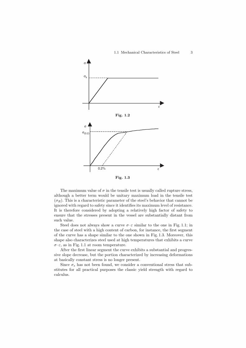
In view of the above considerations, one can replace the curve in Fig. 1.1with that in Fig. 1.2, whereas in a first segment σ is proportional to ε (totallyelastic behavior of material) followed by a segment parallel to the x-axis (per-fectly plastic behavior of the material). Such simplification is most frequentlyused for resistance verification in the elastic–plastic field.

1.1 Mechanical Characteristics of Steel 3

ε

σ

σs

Fig. 1.2

ε

σ

σ(0.2)

0.2%

Fig. 1.3

The maximum value of σ in the tensile test is usually called rupture stress,although a better term would be unitary maximum load in the tensile test(σR). This is a characteristic parameter of the steel’s behavior that cannot beignored with regard to safety since it identifies its maximum level of resistance.It is therefore considered by adopting a relatively high factor of safety toensure that the stresses present in the vessel are substantially distant fromsuch value.

Steel does not always show a curve σ–ε similar to the one in Fig. 1.1; inthe case of steel with a high content of carbon, for instance, the first segmentof the curve has a shape similar to the one shown in Fig. 1.3. Moreover, thisshape also characterizes steel used at high temperatures that exhibits a curveσ–ε, as in Fig. 1.1 at room temperature.

After the first linear segment the curve exhibits a substantial and progres-sive slope decrease, but the portion characterized by increasing deformationsat basically constant stress is no longer present.

Since σs has not been found, we consider a conventional stress that sub-stitutes for all practical purposes the classic yield strength with regard tocalculus.


This is the stress that during the specimen’s release that takes placeaccording to Hooke’s law causes a permanent deformation equal to 0.2%(Fig. 1.3). Therefore, it is indicated with the symbol σ(0.2).

Up to this point, we have discussed the steel’s behavior at room temper-ature. It is, however, of the greatest importance to be aware of the influenceof temperature on the mechanical characteristics of the material.

As we shall see, not only temperature but also time may have a stronginfluence, but right now we shall focus on the effects of temperature on theresults of the classic tensile test.

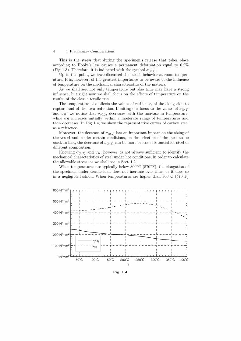
The temperature also affects the values of resilience, of the elongation torupture and of the area reduction. Limiting our focus to the values of σ(0.2)

and σR, we notice that σ(0.2) decreases with the increase in temperature,while σR increases initially within a moderate range of temperatures andthen decreases. In Fig. 1.4, we show the representative curves of carbon steelas a reference.

Moreover, the decrease of σ(0.2) has an important impact on the sizing ofthe vessel and, under certain conditions, on the selection of the steel to beused. In fact, the decrease of σ(0.2) can be more or less substantial for steel ofdifferent composition.

Knowing σ(0.2) and σR, however, is not always sufficient to identify themechanical characteristics of steel under hot conditions, in order to calculatethe allowable stress, as we shall see in Sect. 1.2.

When temperatures are typically below 300◦C (570◦F), the elongation ofthe specimen under tensile load does not increase over time, or it does soin a negligible fashion. When temperatures are higher than 300◦C (570◦F)

0 N/mm2

100 N/mm2

200 N/mm2

300 N/mm2

400 N/mm2

500 N/mm2

600 N/mm2

50˚C 100˚C 150˚C 200˚C 250˚C 300˚C 350˚C 400˚C

σ(0.2)t

σR/t

t

Fig. 1.4

1.1 Mechanical Characteristics of Steel 5

cree

p st

rain

%

transition point

rupture

time

1st period

2nd period

3rd period

Fig. 1.5

the specimen is instead subject to an increased elongation over time; suchelongation is also of variable entity as a function of temperature and stressapplied to it.

Under certain temperature and load conditions the specimen can go intorupture over time. Such phenomenon, called creep, is clearly of great impor-tance for the behavior of vessels over time for both safety and business reasons.If we examine the phenomenon in greater detail (see Fig. 1.5), we notice thatthe strain increases while the elongation’s speed decreases over time until itreaches a minimum value.

This first portion of the curve identifies that which is called the first period.In the second period the elongation’s speed remains practically constant; therepresentative point of the end of the second period is called point of transi-tion. Finally, in the third period the elongation’s speed and the values of thestrain increase rapidly up to the rupture.

Amongst the three analyzed periods, the first and third are rather short,while the second takes most of the total time during which the specimen goesinto rupture. As a reference point, please note that for a total time of about100,000 h the first period represents at most a few hundred hours.

Finally, it is important to understand the great importance played by thepoint of transition that represents the beginning of the short period duringwhich the specimen goes into rupture. The literature sometimes considers itsreference time more important than the rupture time itself. In order to be ableto take into account the creep in the sizing of components working under hotconditions, researchers and institutions initially developed different proposalsthat had in common the characteristic of forecasting tests of short duration,even though they differed with respect to the duration of the test and theevaluation of the results.

In Europe, the most popular proposal came from the German MetallurgicUnion (DVM). Based on the name of this organization, the value of the stressderived from the test was called σDVM and was adopted for some time, andnot only in Germany, to determine the allowable stress at high temperatures.


The stress σDVM is the one that between the 25th and the 35th hourcauses an elongation’s speed inside the specimen not higher than 0.001% h−1

and a permanent deformation after 45 h not greater than 0.2%.The advantage of such tests is the short duration, but they were soon

abandoned, mostly due to the extremely high variability of the values. Infact, the test occurs during the first period of the curve that may have arather variable behavior from casting to casting of the same steel, even whenthe behavior of the curve during the second period is basically the same. Thevalue of σDVM is a poor indicator of the performance of steel over long periodsof time. Thus it became necessary to carry out tests over very long periods oftime.

Nowadays, very many values of specimen made of steel of common usagethat have reached the 100,000 h, and a relevant number of specimen that havebeen tested over even longer periods of time, are available. This allows us todetermine with absolute certainty the behavior of steel of common usage upto 100,000 h of usage. Such is in fact the reference time that is typically takeninto consideration for resistance verification purposes.

The value that is considered for resistance verification is the average ofthe rupture stress for a creep lasting 100,000 h. Such value is indicated withthe symbol σR/100000/t for a generic test temperature t. Note that this is anaverage value: these values are characterized by a certain amount of scatter-ing. We admit that the variability may have a range around the average valueconsidered for calculations equal to no more than 20% of the average valueitself. If the minimum value is outside such range, we shall assume the mini-mum value multiplied by 1.25. If for a given steel and a given temperature weindicate the time on the x-axis and the values of the stress on the y-axis thatcause the rupture of the specimen, which we call σR, in a doubly logarithmicdiagram, we obtain curves that are qualitatively like the one shown in Fig. 1.6.

These curves look like broken lines with more or less evident knees. Thereare also instances – in most cases to be considered exceptional – where suchknees are missing, and the broken line becomes a straight line. Therefore, thevalues of σR/100000/t are derived from these curves for 100,000 h. As we saidabove, for steel of common usage there is no problem given the amount ofvalues for the rupture stress per 100,000 h that are available. The problemsarise when we deal with steel of new fabrication, or that has not yet undergoneextensive tests; in such instances there is nothing else to do but to extrapolateon the basis of the values known for shorter periods of time. The extrapolationis possible with all the necessary cautionary tales, but it is sufficiently reliableonly if it is not pushed too far. This is because of the presence of the knees, andalso because even a small mistake in the determination of the values relatedto longer experimental time frames would result in substantial errors in thevalues obtained through extrapolation.

An acceptable extrapolation should not involve a timing ratio greater than10; limiting such ratio to five leads to values that are sufficiently reliable.

1.2 Allowable Stress 7

50

60

708090

100

200

300

400

100 1000 10000 100000

time [h]

Fig. 1.6

In other words, to obtain reliable values for 100,000 h the longest test shall beat least of 20,000 h.

1.2 Allowable Stress

The following stresses are typically considered to determine the basic allowablestress of steel:

σR = minimum value of the unitary maximum load during the tensile test(rupture stress) at room temperature.σ(0.2)/t = minimum value of the unitary load during the tensile test attemperature t with a permanent deformation equal to 0.2% of the initiallength between references after removal of load.σR/100000/t = average value of the unitary rupture stress for creep after100,000 h at temperature t.

In the case of austenitic steel there is general agreement that instead of apermanent deformation of 0.2% we refer to a deformation of 1%. Note thatthe temperature t is the average wall temperature.

As discussed in Sect. 1.1, the meaning of these values is certainly clear tothe reader; this not withstanding, further clarifications are due.

The rupture stress during the tensile test refers to room temperature.This may sound surprising since the resistance verification must be executedat design temperature t, to which the other two values above in fact refer.As pointed out in Sect. 1.1, the value of the rupture stress at moderate


temperatures is greater than the one at room temperature. Within this tem-perature range, the adoption of this last value addresses basic safety criteria.The use of this value is in fact justified within the range of moderate tem-peratures: the goal here is to guarantee, through an adequate safety factor(as we shall see later on), that stresses acting upon the vessel do not cause adangerous situation leading to rupture. Moreover, the value of σR is at timescrucial, as far as allowable stress is concerned, when steel with high levels ofyield strength are adopted. In this case if the design temperature is eitherroom temperature or anyway moderate, the value of σ(0.2)/t is very close toσR. The determination of the allowable stress solely based on σ(0.2)/t may leadto a value that does not sufficiently protect against rupture.

Considering now the unitary load that causes a permanent deformation of0.2% at release during the tensile test (we use the symbol σ(0.2)/t to rememberthat one should refer to the design temperature t), we pointed out in Sect. 1.1that it practically replaces the yield strength when the steel does not exhibitthe classic yielding phenomenon. If, on the other hand, this were the case, itwould be easy to determine, due to the entity of the resulting deformations,that the value of σ(0.2) coincides with the lower value of the yield strength.

We shall use the symbol σs instead of σ(0.2)/t in the following chapters forsimplicity purposes. The latter is in most cases crucial to determine the valueof allowable stress. We will also use the term “yield strength”, even though itis formally incorrect, to simplify the language. Finally, as far as the rupturestress per creep at 100,000 h is concerned, its importance is now evident, inview of what discussed in Sect. 1.1, if the design temperature is high. For suchstress, given the dispersion of values present even for similar types of steel,one refers to the mean value of the range, generally assuming that the size ofthe range itself does not go beyond ±20%.

In order to obtain the allowable stress, the three characteristic stresses areassociated to safety factors, the values of which lack a general consensus, andthat have undergone numerous modifications over time. The general trendhas been to reduce them, as the behavior of different kinds of steel becamebetter understood, to require more stringent inspections and refine calculationmethodologies. We therefore recommend the following criterion that will beapplied throughout the book.

The basic allowable stress of the material that from now on we will call fis given by the smallest of the following values:

σR

2.4,

σ(0.2)/t

1.5, and

σR/100,000/t

1.5.

From a conceptual point of view, the basic value is the one derived fromσ(0.2)/t. For this reason, we will always refer to the yield strength when wehave to correlate the allowable stress with a value typical of the material’sresistance. The other two values mentioned above occur in special instances,even though σR/100000/t is found quite frequently.

1.3 Theories of Failure 9

We have already discussed elsewhere the reasons that suggest to take σR

into consideration. σR/100000/t is critical for f when its value is lower than theyield strength, since the safety factor has the same value of the one relativeto σ(0.2)/t. For instance, this happens for carbon steel at temperatures be-yond 380–420◦C (715–790◦F), for low-alloy steel at temperatures higher than470–500◦C (880–930◦F), and for austenitic steel at temperatures higher than500◦C (930◦F).

Finally, note that we have defined the stress f as basic allowable stressof the material. This does not necessarily mean that it corresponds to theallowable stress during resistance verification of a specific piece in a specificposition.

As we shall often return to this, in some cases it is acceptable that theideal stress may reach the yield strength or even, in spite of being physicallyimpossible, twice the yield strength (only from the point of view of calculationin the elastic field). We will discuss this issue in Sects. 1.4 and 1.5. The stressf , which in other cases actually corresponds to the maximum stress allowablefor the piece, and at any rate to the maximum ideal stress of the membrane,represents a reference point, since it is present in all equations to compute thethickness of the various components. As a matter of fact, even when greaterallowable values are assumed, they are correlated to the value of f .

1.3 Theories of Failure

This is a widely discussed topic in construction theory. In this book it isneither necessary nor relevant to examine all failure theories. We shall limitourselves to consider those that directly relate to resistance verification ofpressure vessels, and even for these we will highlight only those aspects thatare required to understand what follows next.

Pressure vessels are characterized by the existence of stresses along threeaxis. First of all, due to pressure, there is a principal stress directed as thepressure itself and thus orthogonal to the wall of the vessel, while two addi-tional principal stresses act on the plane orthogonal to the previous one.

In the case of cylindrical elements the first of such stresses is radial, theother two are directed, respectively, along the circumference and along theaxis of the cylinder.

Similarly, in the case of spherical elements the first stress is radial, theother two are directed, respectively, along the meridian and the circumferenceorthogonal to the meridian, and they are obviously identical.

Different situations may occur with elements that are neither cylindricalnor spherical, e.g., in the case of a flat head the first of the three stressesmentioned above is orthogonal with respect to the head, and therefore alongthe same direction of the axis of the vessel, if the flat head is orthogonal tothe latter. The other two have circumferential and radial direction.


In any case, we are faced with a state of stresses along three axis. Thiscalls for a failure theory that allows one to correlate such state of stress withthe resistance values of the material, derived from the tensile test that in turnis based on a single stress directed along the axis of the specimen.

The most generally accepted failure theories for ductile materials, such assteel used to build pressure vessels, are the well-known theory of maximumshear stress or Guest–Tresca, and the one known as distorsion energy theoryor Huber–Hencky.

According to Guest–Tresca the level of danger is captured by the maxi-mum shear stress, in other words all states having the same maximum shearstress are equivalent with respect to danger. The state of stress relative tothe specimen being subjected to single tensile stress is represented in Mohr’splane by the only circle shown in Fig. 1.7. The maximum shear stress actingat 45◦ with respect to the only principal stress σIII is equal to σIII /2.

Therefore, if we associate a dangerous condition to the yielding of thematerial and we call σs the corresponding stress, the shear stress is given by

τs =σs

2. (1.1)

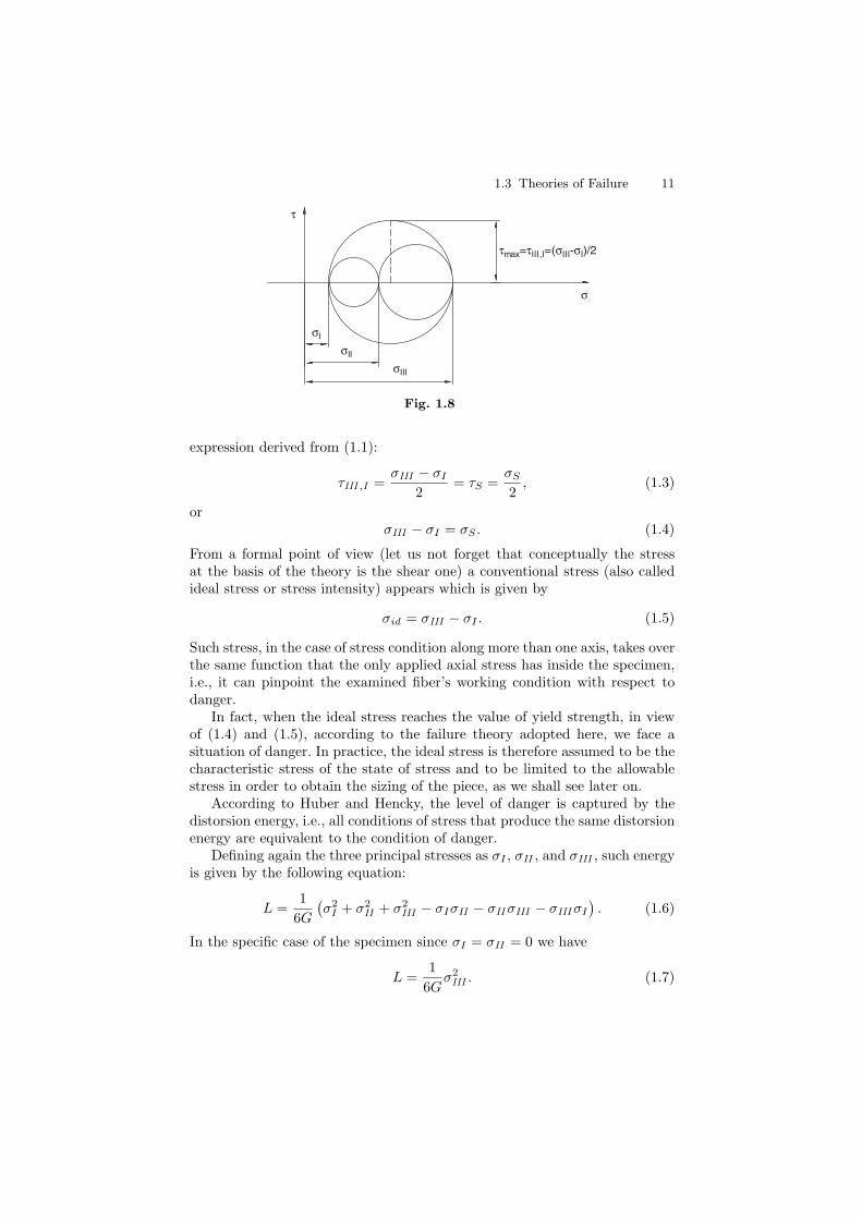
If the state of stress is along three axis, and we call σI , σII , and σIII the threeprincipal stresses, let us agree that the three increase in value from σI to σIII

(see Fig. 1.8).The three maximum shear stresses on the three planes where they operate

are hence given, respectively, by

τIII ,I = (σIII − σI) /2;τIII ,II = (σIII − σII ) /2; (1.2)τII ,I = (σII − σI) /2.

With the above agreement the maximum value of the shear stress is given byτIII .I and therefore the condition of danger is represented by the following

τmax=σIII /2

σIII

σ

τ

Fig. 1.7

1.3 Theories of Failure 11

τmax=τIII,I=(σIII-σI)/2

σ

τ

σII

σIII

σI

Fig. 1.8

expression derived from (1.1):

τIII ,I =σIII − σI

2= τS =

σS

2, (1.3)

orσIII − σI = σS . (1.4)

From a formal point of view (let us not forget that conceptually the stressat the basis of the theory is the shear one) a conventional stress (also calledideal stress or stress intensity) appears which is given by

σid = σIII − σI . (1.5)

Such stress, in the case of stress condition along more than one axis, takes overthe same function that the only applied axial stress has inside the specimen,i.e., it can pinpoint the examined fiber’s working condition with respect todanger.

In fact, when the ideal stress reaches the value of yield strength, in viewof (1.4) and (1.5), according to the failure theory adopted here, we face asituation of danger. In practice, the ideal stress is therefore assumed to be thecharacteristic stress of the state of stress and to be limited to the allowablestress in order to obtain the sizing of the piece, as we shall see later on.

According to Huber and Hencky, the level of danger is captured by thedistorsion energy, i.e., all conditions of stress that produce the same distorsionenergy are equivalent to the condition of danger.

Defining again the three principal stresses as σI , σII , and σIII , such energyis given by the following equation:

L =1

6G

(σ2

I + σ2II + σ2

III − σIσII − σII σIII − σIII σI

). (1.6)

In the specific case of the specimen since σI = σII = 0 we have

L =1

6Gσ2III . (1.7)


The condition of danger characterized by σIII = σs corresponds to a distorsionenergy equal to

Ls =1

6Gσ2

s . (1.8)

For a state of stresses along more than one axis the condition of danger istherefore given by

L = Ls =1

6Gσ2

s . (1.9)

From (1.6) and (1.9) we obtain√

σ2I + σ2

II + σ2III − σIσII − σII σIII − σIII σI = σs. (1.10)

Therefore, also in this case an ideal stress is determined

σid =√

σ2I + σ2

II + σ2III − σIσII − σII σIII − σIII σI . (1.11)

This ideal stress relates to the stress state and allows one to identify theworking condition of the fiber under scrutiny. As for the previously discussedtheory, when σid reaches the value of the yield strength a dangerous conditiontakes place, according to (1.10) and (1.11). Similarly, the sizing of the pieceis obtained by making sure that σid does not go beyond the allowable stress.

According to von Mises, the condition of danger depends on the value ofthe following conventional stress:

τid =√

τ2III ,I + τ2

III ,II + τ2II ,I . (1.12)

It must not go above a threshold that depends on the average value of theprincipal stresses given by

σm =σI + σII + σIII

3. (1.13)

If we rule out the dependency of the value of danger of τid on σm, we realizethat von Mises’ theory formally corresponds to Huber–Hencky’s, in the sensethat the ideal stress σid is the same as that in (1.11).

In fact, on the basis of (1.2) we obtain from (1.12):

τid =1√2

√σ2

I + σ2II + σ2

III − σIσII − σII σIII − σIII σI . (1.14)

In the case of the specimen

τid =1√2σIII , (1.15)

and the condition of danger is reached when σIII = σs.

1.4 Plasticity Collaboration 13

By replacing σIII with σs in (1.15), and by comparing it with (1.14), weobtain (1.10). The ideal stress is represented by (1.11) in this case as well.Therefore, it is customary to talk about failure theory of Huber–Hencky–vonMises every time (1.11) is adopted, even though, as we have seen above, vonMises starts from assumptions that are completely different from a conceptualpoint of view.

Today this theory is the most generally accepted for resistance verificationof pieces for which ductile materials are used, more than the Guest–Trescatheory. Note, though, that codes in the most important industrialized coun-tries are based on the theory of Guest–Tresca.

The reason for this is because the theory of Guest–Tresca is more con-servative than that of Huber–Hencky and easier to apply as well, as one canimmediately realize by comparing the equations of σid in both cases.

We will generally refer to this theory of failure as well, without neglect-ing to refer to the theory of Huber–Hencky, however, every time it will benecessary or appropriate.

1.4 Plasticity Collaboration

In the sizing of pressure vessels the possibility of plastic collaboration of steelis widely exploited. This is a topic that, if dealt with in great depth, wouldresult in a vast analysis that is in fact not justified considering what is ofpractical interest for resistance verification, a topic we will shortly introduce.Therefore, we will concentrate on reviewing the fundamental concepts by mod-eling the problems in a simple way, and by analyzing only those aspects ofthe phenomenon that find actual application in the analysis presented in thecoming chapters.

The principle at the core of plastic collaboration consists of the possibilitythat less stressed fibers may contribute to the resistance of the piece by helpingthe most stressed ones. More precisely, the adoption of the criteria of plasticcollaboration goes against the traditional concept of verification in the elasticfield, which says that the condition of danger is reached when the most stressedfiber begins to show signs of yielding in the material. If the material is ductileit can withstand major deformations before rupturing. Therefore, the fact thatthe material yields in one area of the piece does not represent a condition ofdanger, if the nearby fibers are still far from yielding.

Let us consider a simplified stress–deformation curve, as is usually donein this cases, as in Fig. 1.9. The intuition is that the behavior of the steel iselastic–plastic, where the first section of the curve shows a perfectly elasticbehavior, while the second section is parallel to the axis of deformations (i.e.,a perfectly plastic behavior). In other words, we ignore the hardening, whichactually has a favorable effect on resistance, and we assume that the materialshows substantial yielding.


ε

σ

σs

Fig. 1.9

Once yielding in a portion of the piece is reached, if we increase the externalforces acting on the piece itself (in our case it is generally the pressure),the yielded fiber or fibers are unable to absorb another increase in stress.They undergo an increase in deformation, but the stress remains constant.At the same time, the nearby fibers that are still far from yielding are ableto absorb increasing stresses. These are greater than those derived from cal-culation in the elastic field because of the greater deformation following theyielding of nearby fibers or, operating within an equilibrium framework, giventhe requirement to balance the increase in external forces for which the yieldedfibers are no longer able to provide a contribution.

The condition of danger is reached when all fibers have exhausted thepossibility to absorb an increase in stress; in other words, the condition ofdanger is represented by the plastic flow of the entire piece. At this point,while peaks of deformation are present given the constraint to the conditionsof congruence, peaks of stress have disappeared since in every point the stressis equal to the yield strength. Following this simplified model, taking intoaccount plastic collaboration corresponds in practice to ignoring the peaks ofstress.

This issue is in fact more complex since there is vast case history, andevery stress condition should be examined separately through a process knownas stress analysis. This helps to identify the exact nature of the peak, inorder to determine which criteria to apply to carry out verification. Suchprocedure can be found, e.g., in Sect. III of the ASME Code that deals with theverification of nuclear vessels, where the responsibility of the investigation ofthe stress condition is left to the designer. This can be done through traditionalcomputational methodologies, if the theoretical modeling of the problem ispossible, or through investigation criteria that are nowadays possible with thehelp of a computer and finite element analysis techniques.

The ASME code indicates at this point which criteria should be used todetermine whether the values of stresses are compatible with the safety ofthe vessel, based on the nature of the stresses themselves, including general


and local membrane stresses, those concerning bending, self-limiting ones,etc. We will focus on this topic in detail in Sect. 1.5 when we introduce themodern criteria of verification. We shall refer to them in the next chapterswhen we examine those cases that lend themselves to a theoretical analysisof the problem. Through the criteria illustrated in Sect. 1.5, we shall findconfirmation to what stated in the beginning, i.e., the exploitation of plasticcollaboration of the material according to various criteria that indeed dependon the different nature of peaks.

To understand the philosophy at the basis of the criteria in Sect. 1.5, itis therefore appropriate to try to model the most frequent situations. Fromthis point of view a number of considerations can be made. The verificationmay involve a component for which an average stress not equal to zero or notlocalized is clearly identifiable. This is the case, for instance, of stresses ina cylinder subject to pressure from the inside without holes, or, if holes arepresent, in areas of the same but at such distance from the holes not to beinfluenced by them. In this case, as we shall see, the circumferential and theradial stress vary with the radius through the wall. Their difference representsthe ideal stress according to Guest. This has a value that varies across the walland shows a nonzero average value. With respect to the average value, theideal stress shows both positive and negative peaks that are going to disappearif the cylinder becomes plastic, since the average stress, if ideally distributedover the entire thickness, is able to balance the acting pressure.

The methodology of plastic collaboration corresponds to neglecting thesepeaks by doing the calculations on the base of average values for the stresses.As we shall see, in the case at hand it is also possible to define a mathematicalformulation of the distribution of stresses under total plastic conditions. Thismakes it possible to reason on such boundary situation by examining theresistance of the piece from a global viewpoint. Similar situations occur if thereare drilling lines with holes that are so close to be considered non isolated, aswe shall discuss in more detail later on. Even in this case the circumferentialstress between holes, and in some instances the longitudinal stress as well,shows significant peaks in correspondence of the holes’ edges. Adopting thecriteria of plastic collaboration, these peaks are neglected by referring in thecalculation to the average value of stresses that occur between holes.

A completely different situation occurs when stresses through the wallshow a change in sign. In this case the average value may be even zero if thereis pure bending. In reality this never takes place because of the simultaneouspresence of stresses with a constant sign that overlap those caused by thebending. The average value is by the way very small with respect to themaximum values for stresses due to the clearly prevailing bending moment.

An example of this is a flat head or a vessel with a quadrangular section.It is obvious that even adopting plastic collaboration, one cannot here referto the average value of stresses since it does not balance the external actingforces.


b

a σmax<σs σs

F

F b/2

Fig. 1.10

Let us consider at this point how plastic collaboration occurs on a beamwith a rectangular section under pure bending, as in Fig. 1.10.

In the elastic field stresses behave as shown on the left side of the figure.When increasing the bending moment up to the total plastic flow, the firstfibers to yield are the external ones; subsequently, the yielding moves moreand more towards the neutral axis, until the diagram becomes as shown onthe right side of the figure.

At the limit of elastic behavior the moment is equal to

Me = Wσs =16ab2σs, (1.16)

where W is the section modulus. When the section is completely yielded, thecorresponding moment is equal to

Mp = Fb

2= a

b

2σs

b

2=

14ab2σs. (1.17)

The coefficient of plastic collaboration is therefore given by the relationshipbetween these two moments that represent the condition of danger, accordingto the calculation that takes plastic collaboration into account, and accord-ing to traditional computation practices in the elastic field, respectively. Byindicating the coefficient of collaboration with ψ we have:

ψ =Mp

Me= 1.5, (1.18)

a well-known value in the literature. As far as stress peaks that occur incorrespondence with isolated holes, the most appropriate way to approachthe problem consists of examining the stress status around the edge of thehole in detail, and to apply the verification criteria discussed in Sect. 1.5.

If we are unable or do not want to perform such analysis, it is possible toadopt the criteria discussed in Chap. 8 that have been included with minorvariations in the codes of the most industrialized countries for non-nuclear


pressure vessels. As we shall see, even in this case plastic collaboration isfactored in, by limiting the width of the area where the fibers collaboratewith those subjected to most stress. In doing so, a limit is set to deformationsin correspondence of peaks. In fact, an indiscriminate extension of the yieldingto fibers far from reaching a peak, with regard to danger, would imply theonset of large deformations in correspondence with the peak itself, somethingclearly to be avoided.

It is also important to consider those peaks that are the consequence of therespect for congruence of deformations among pieces of different geometricalshape connected with each other. If they were ideally isolated, they would becharacterized by different values of deformations in correspondence with thejunction. Heads (whether flat, hemispherical or torospherical) connected tothe ends of the cylinders represent a typical case.

In these cases, the stresses are, as we usually say, self-limiting, since theyoccur only out of necessity to respect congruence, and not to balance externalforces. If we reach the yielding point and the subsequent deformations are rela-tively large, congruence is maintained without leading the material to rupture.

In fact, in these situations it would be more logical to carry out the analysisin terms of deformations. In practice this is done according to the laws ofelasticity and peak stresses are obtained. We should also not forget the natureof such stresses, and we should not be surprised, if values for stress higher thanthe yield strength are introduced, which may seem absurd.

That is, the peak deformation takes on a value greater than that of theyield strength. The stress resulting from the calculation is greater than σs onlyfrom a formal point of view, as the product of deformation by the modulus ofelasticity; in reality, it is obvious that the stress is equal to σs.

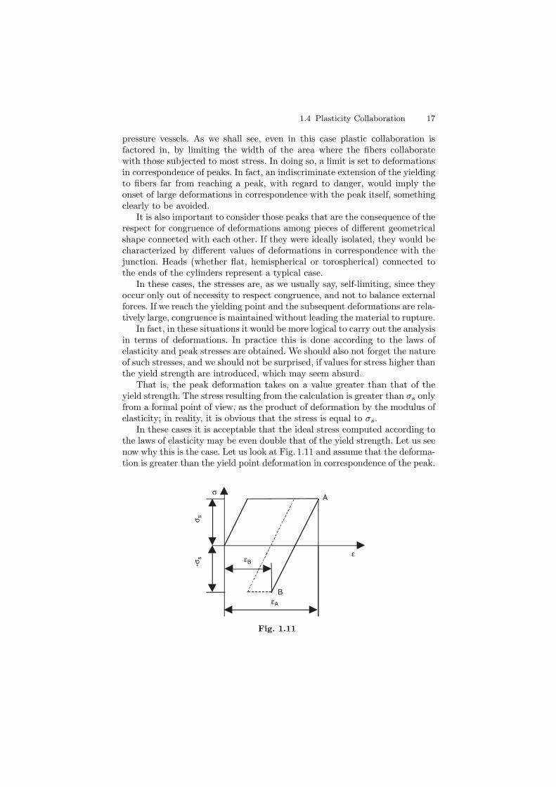
In these cases it is acceptable that the ideal stress computed according tothe laws of elasticity may be even double that of the yield strength. Let us seenow why this is the case. Let us look at Fig. 1.11 and assume that the deforma-tion is greater than the yield point deformation in correspondence of the peak.

σ

σ s

B

A

-σs

εεB

εA

Fig. 1.11


The deformation is εA in correspondence of point A on the typical curve forperfectly elastic–plastic material. At release the material behaves elastically,and we also assume that the residual deformation is εB in correspondence ofpoint B, and a residual stress equal to the negative yield strength.

If we next load the piece, we return to point A, and every subsequentcycle causes the stress to vary between −σs and σs. In other words, exceptfor the first cycle, for all the following ones the piece’s behavior is elasticbetween point A and B, without further deformations since εA constitutesthe deformation that takes congruence into account.

In order for this condition to occur, it is necessary and sufficient that thestress, computed according to the laws of elasticity, be double than the yieldstrength. Of course, if it happens to be lower the behavior of the material iscompletely analogous with the only difference that during release the negativeyield strength is not reached. If, conversely, the stress should be more thandouble the yield strength, we would have the cycle that appears dashed inthe figure. The material would therefore have an elastic–plastic behavior inthose cycles following the first one, with the danger that incremental plasticdeformations occur that the adopted model does not seem to justify, but thatmay actually happen in reality.

The calculation criterion introduced here is not limited to the junctions ofpieces of different geometrical shape, but can be extended in general to all thosesituations where stresses originate from noncongruent deformations. Therefore,even the stresses due to thermal flux fall into this category, i.e., those stressescaused by variable thermal expansion through the wall of the piece. To con-clude, it is noteworthy that the exploitation of plastic collaboration and thederiving lack of interest in peaks is possible and appropriate not only in rela-tion with the type of steel used, but due to the absence of fatigue phenomena.

When an investigation about fatigue is required, the verification criteriaare obviously different, and this is discussed in Sect. 1.5. Moreover, it is impor-tant to keep in mind that the verification criteria and the deriving equationsfor sizing discussed in the following chapters refer to work conditions thatdo not imply significant fatigue phenomena, due to the presence of a limitednumber of cycles.

If this were not the case, the validity of the equations to calculatethe stresses that take peaks into account notwithstanding (thus ruling outthe equations that consider the components of the vessel as membranes), theverification criteria must follow what discussed in Sect. 1.5 and in more detailin Chap. 10.

1.5 Verification Criteria

According to modern verification criteria, stresses can be divided into threecategories: primary, secondary, and peak stresses. Primary stresses can then bedivided into general membrane stresses, local membrane stresses, and primary

1.5 Verification Criteria 19

bending stresses. In summary, there are the following types of stresses: generalmembrane, local membrane, primary bending, secondary, and peak.

1.5.1 General Membrane Stresses (σm)

They correspond to stresses derived from calculation when one considers theelement under test as a membrane. More generally, they correspond to theaverage value of the stresses through the thickness of the vessel. In contrastto local membrane stresses, that we will discuss shortly, the fundamental char-acteristic of these stresses is that a potential yielding of the material does notcause a redistribution of the stresses, since the same stress is present in allthe surrounding fibers.

A typical example of general membrane stresses is represented by theaverage values of the stresses acting in a cylinder without holes (or in anarea that is not influenced by holes or by the junction with the heads). Thesame is true for the average values of the stresses acting on a sphere, or in thecentral area of a hemispheric or torospherical head.

1.5.2 Local Membrane Stresses (σml)

Here as well we are dealing with the average values of the stresses throughthe thickness in the analyzed section. In contrast with the previous ones, theyinvolve a limited area of the component, and this means that the surroundingfibers are subject to membrane stress of lower value. A potential yieldingof the material happens together with a redistribution of the stresses to thesurrounding fibers that are still able to contribute to the local resistance ofmaterial, since they are not yielded.

Typical examples of stresses of this kind are the membrane stresses pro-duced in the cylinder and in the dished heads in correspondence with theirjunction, or the membrane stresses that occur in the cylinder (or in thesphere), and in the nozzle welded on the same in correspondence of a hole.

Once again, these are the average values of the stresses. Stress peaks bothin the junction cylinder-heads and in correspondence of the nozzles are gen-erated that do not fall into this kind of stress category.

1.5.3 Primary Bending Stresses (σf)

These stresses belong to the category of primary stresses, such as the onesmentioned above, but they are characterized by the fact that their value isproportional to the distance of the fiber from the neutral axis of the section. Asthe previous ones, they derive from the balance conditions between internalstresses and external forces acting upon the vessel (pressure or mechanicalloads). A typical example is represented by the stresses at the center of a flathead. The stresses produced by bending moments exerted on a vessel with aquadrangular section fall into this category, as well.


At this point we must discuss a very important concept in more detail.A bending moment may also generate a distribution of stresses that do notvary linearly across the thickness. An example can be seen at the cornersof a vessel with a quadrangular section. Here, the primary bending stressesare those that balance the acting moment with linear variation throughthe thickness. With respect to these, the stresses that are actually presentin the section, display positive or negative differences characterized by aresultant and a moment that are zero. These differential stresses do not bal-ance the forces applied to the vessel, but only guarantee the congruence ofthe deformations. Therefore, they fall into the category of secondary stresses.The analogy with membrane stresses is evident: the latter ones represent theaverage value of the stresses produced by a normal load. The primary bend-ing stresses represent the average behavior of the stresses caused by a bendingmoment.

The differential stresses versus the membrane ones (in the presence of anormal load), or with respect to the primary bending stresses (in the presenceof a bending moment), are secondary stresses.

1.5.4 Secondary Stresses (σsec)

Their fundamental characteristic is not to be involved in balancing the forcesapplied to the vessel, and to be for this reason self-limiting. Their only purposeis to guarantee the congruence of the deformations and, therefore, once therequired deformations are produced (even though this happens through theyielding of the material) they do neither cause further deformations nor dothey force the intervention of the surrounding fibers, as is the case instead forthe local membrane stresses.

The stresses in correspondence of the junction between cylinder and headsbelong to this category (not the membrane ones because in that case theyare local membrane stresses); the stresses still not related to membranes inthe cylinder or in the sphere and in the welded nipple in correspondenceof a hole belong to this category, as well. In this last case local peaks dueto the presence of sharp edges are excluded, as they belong to the nextcategory.

The stresses due to thermal flux are secondary, as well. In fact, they are alsoself-limiting, since they are produced solely to reestablish the congruence ofthe deformations that differ in the various fibers because of the temperaturegradient. Even though they originate elsewhere, some differences in stresslevels also belong to this category (with respect to the average value thatrepresents the general membrane stress); they occur in a cylinder or a sphere,especially in the case of great thickness, along the radius. These differences instress do not contribute to balancing the pressure (as the balance is guaranteedby the general membrane stress), but only to ensure the congruence of thedeformations.

pressure vessel design - download.e-bookshelf.de · speciﬁcally, pressure vessels represent...

Documents