presented by: erik cox, shannon hintzman, mike miller, jacquie otto, adam serdar, lacie zimmerman

Presented by:Erik Cox, Shannon Hintzman,

Mike Miller, Jacquie Otto,

Adam Serdar, Lacie Zimmerman

deadalivecat 2

1

What’s to come…

-Brief history and background of quantum mechanics and quantum computation

-Linear Algebra required to understand quantum mechanics

-Dirac Bra-ket Notation

-Modeling quantum mechanics and applying it to quantum computation

History of Quantum Mechanics

Sufficiently describes everyday things and events.

Breaks down for very small sizes (quantum mechanics) and very high speeds (theory of relativity).

Classical (Newtonian) Physics

Why do we need Quantum Mechanics?

In short, quantum mechanics describes behaviors that classical (Newtonian) physics cannot. Some behaviors include:

- The wave-particle duality of light and matter

- Discreteness of energy

- Quantum tunneling- The Heisenberg uncertainty principle

- Spin of a particle

Spin of a Particle- Discovered in 1922 by Otto Stern and

Walther Gerlach

- Experiment indicated that atomic particles possess intrinsic angular momentum, called

spin, that can only have certain discrete values.

The Quantum Computer

Idea developed by Richard Feynman in 1982.

Concept:Create a computer that uses the effects of quantum mechanics to its advantage.

Classical Computer

Information

Quantum Computer

Informationvs.

- Bit, exists in two states, 0 or 1

- Qubit, exists in two states, 0 or 1, and superposition of both

Why are quantum computers important?

Recently, Peter Shor developed an algorithm to factor large numbers on a quantum computer. Since factoring is key to current encryption, quantum computers would be able to quickly break current cryptography techniques.

In the beginning, there was Linear Algebra…

- Complex inner product spaces

- Linear Operators

- Unitary Operators

- Projections

- Tensor Products

Complex inner product spaces

njCzzzzzC jnn ..1,|,...,,, 321

An inner product space is a complex vector space , together with a map f : V x V → F where F is the ground field C. We write <x, y> instead of f(x, y) and require that the following axioms be satisfied:

V

,0,, xxVx and iff0, xx 0x

yzxzayaxzVzyxFa ,,,,,,,

*,,,, xyyxVyx

denotes complex conjugate*

(Positive Definiteness)

(Conjugate Bilinearity)

(Conjugate Symmetry)

Complex Conjugate:

iyxz iyxz *

1iwhere

njCzzzzzCV jnn ..1,,...,,, 321

Example of Complex Inner Product Space:

Cz Let

Vwv ,Let

nn wvwvwvwv *...**, 2211

Linear Operators

Example:

xgdxdxfdxdxgxfdxd ///

xfdxdcxcfdxd //

yAxAyxA ˆˆˆ (Additivity)

xAcxcA ˆˆ (Homogeneity)

Let and be vector spaces over , then is a linear operator if . The following properties exist:

V WWVA :ˆ

Vyx ,

C,Cc

Unitary Operators

tUU 1

IUUUU tt

t denotes adjoint

Properties:

Norm Preserving…

Inner Product Preserving…

AdjointsMatrix

Representation

nnnnn

n

n

aaaa

aaaa

aaaa

A

...

...

...

...

321

1322212

1312111

nnnnn

n

n

t

aaaa

aaaa

aaaa

A

*...***

...

*...***

*...***

321

1232221

1131211

Suppose VwvVVU ,,:

wvAwAv t Definition of Adjoint:

wvUUwUvU t

wvwvI

(Inner Product Preserving)

vvvvUvUvU (Norm

Preserving)

• In quantum mechanics we use orthogonal projections.

• Definition: Let V be an inner product space over F. Let M be a subspace of V. Given an element then the orthogonal projection of y onto M is the vector which satisfies

where v is orthogonal to every element .

Vy MPy

vPyy Mm

A projection operator P on V satisfies

We say P is the projection onto its range, i.e., onto the subspace

2PPP t

vPvVvW :

In quantum mechanics tensor products are used with :

• Vectors• Vector Spaces• Operators• N-Fold tensor

products.

If and , there is a natural mapping defined by

We use notation w v to symbolize T(w, v) and call w v the tensor product of w and v.

mCW nCV mnCVWT :

nmnnm yyxyyxyyxxT ,...,,...,,...,,...,,,..., 11111

nmmn yxyxyxyx ,...,,...,,..., 1111

• W V means the vector space consisting of all finite formal sums:

where

and

jiij vwa Wwi Vv j

If A, B are operators on W and V we define AB on WV by

jiijjiij BvAwavwaBA

4 Properties of Tensor Products

1. a(w v) = (aw) v = w (av) for all a in C;

2. (x + y) v = x v + y v;

3. w (x + y) = w x + w y;

4. w x | y z = w | y x | v .

Note: | is the notation used for inner products in quantum mechanics.

Property #1: a(w v) = (aw) v = w (av) for all a in C

Example in :

2C),,,()( 22122111 vwvwvwvwavwa

),,,( 22122111 vawvawvawvaw

Example in :2C

vwwavaw ),()( 21

vawaw ),( 21


Example in :2C

),()( 21 vvawavw ),( 21 avavw


Property #2:

(x + y) v = x v + y v

Example in :2C

vyyxxvyx )),(),(()( 2121

))),((),),((( 221121 vxxvxx

),,,( 22211211 vxvxvxvx

))),((),),((( 221121 vyyvyy

),,,( 22211211 vyvyvyvy

Example in :

),,,( 22122111 vxvxvxvxvyvx

),,,( 22122111 vyvyvyvy

2C

Property #3:

w (x + y) = w x + w y

Example in :2C

)),(),(()( 2121 yyxxwyxw

))),(()),,((( 212211 xxwxxw

),,,( 22122111 xwxwxwxw))),(()),,((( 212211 yywyyw

),,,( 22122111 ywywywyw

2C),,,( 22122111 xwxwxwxwywxw

),,,( 22122111 ywywywyw

Example in :

Example in :2C zxyw ||

))(*)()(*)(( 2211 ywyw ))(*)()(*)(( 2211 zxzx

),(|),(),(|),( 21212121 zzxxyyww

)))((*)(*)(())(*))((*)(( 22211111 yzxwzxyw

)))((*)(*)(())(*))((*)(( 22221122 yzxwzxyw

)(*)()(*)( 21211111 zyxwzyxw )(*)()(*)( 22221212 zyxwzyxw

Dirac Bra-Ket NotationNotation

Inner Products

Outer Products

Completeness Equation

Outer Product Representation of Operators

Bra-Ket Notation Involves

Bra

<n| = |n>t

Ket

|n>

Vector Xn can be represented two

ways

z

y

x

w

v ***** zyxwv

*m is the complex conjugate of m

Inner ProductsAn Inner Product is a Bra multiplied by a Ket

<x| |y> can be simplified to <x|y>

<x|y> =

p

o

n

m

l

= ***** zyxwv***** pzoynxmwlv

Outer ProductsAn Outer Product is a Ket multiplied by a Bra

|y><x| =

p

o

n

m

l

=

*****

*****

*****

*****

*****

pzpypxpwpv

ozoyoxowov

nznynxnwnv

mzmymxmwmv

lzlylxlwlv

***** zyxwv

By Definition xvyvyx

Completeness Equation

vivivii ||||||

So Effectively

Iii ||

Let |i>, i = 1, 2, ..., n, be a basis for V

and v is a vector in V

is used to create a identity operator represented by vector products.

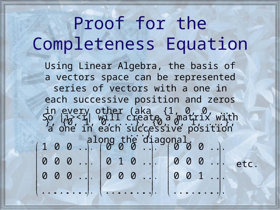
Proof for the Completeness Equation

Using Linear Algebra, the basis of a vectors space can be represented series of vectors with a one in each successive position and zeros in every other (aka {1, 0, 0, ... }, {0, 1, 0, ...}, {0, 0, 1, ...}, ...)

So |i><i| will create a matrix with a one in each successive position along the diagonal.

............

...000

...000

...001

............

...000

...010

...000

............

...100

...000

...000

etc.

Completeness Cont.Thus

|| ii =

............

...000

...000

...001

............

...000

...010

...000

............

...100

...000

...000

+ + + ... =

............

...100

...010

...001

= I

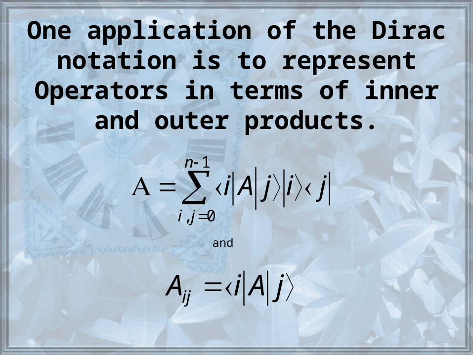
One application of the Dirac notation is to represent

Operators in terms of inner and outer products.

1

0,

n

ji

jijAi

jAiAij

and

• If A is an operator, we can represent A by applying the completeness equation twice this gives the following equation:

• This shows that any operator has an outer product representation and that the entries of the associated matrix for the basis |i are:

1

0,

n

ji

jijAi

jAiAij

Projections

• Projection is a type of operator• Application of inner and outer

products

Linear Algebra View

x

yv

u

yxv We can represent

graphically:

0yxUsing the rule of dot products we

know

ucx0cGiven that we can say

Linear Algebra View (Cont.)Using these facts we can solve

x

y

for and

uyucuv )(

uyuucuyuc )(

yucv

0yu�

Again using the rule of dot products2

ucuv We get

Linear Algebra View (Cont.)

2u

vuc

So

uu

vuvxvy

2

uu

vux

2

Plugging this back into the original equation

Gives us:

ucx

Linear Algebra View (Cont.)

1u

If is a unit vector u

uvux�

)( uvuvy�

)(

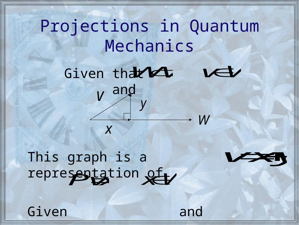
Projections in Quantum Mechanics

VW VvGiven that and

x

yvW

xPv Wxyxv This graph is a representation of

Given and

Projections in QM (cont.)

k,...2,1 being the full basis of W

}|,...1|,|,...2|,1{| nkk

We can regard the full basis of as being

V

nckc

kcccv

nk

k

|...1|

|...2|1|

1

21On Basis

Cc j For some


ncccv n 1...21111 21

Taking the inner products gives

n

kj

n

j

n

j

jvjjvjjvjv111

vjc j Therefore and more

generally

vc 11 So


Wjvjxn

j

1

n

kj

jvjy1

Now set

k

j

jjP1

k

j

k

j

vjjjvjPv11

So

Computational Basis2CV

n

VVVVV n 2222 ...

Basis for 2CV

)0,1(0 )1,0(1

1,0

Computational Basis (cont.)

2CA basis for will have basis vectors:

nV Called a computational basis

1...11,...,10...00,01...00,0...00

10...0001...00 Notation:

Quantum States

22,12,1 : Czzzz

Thinking in terms of directions

model quantum states by directions in a vector space

1

0 1z

2z

1,0

0,1

Associated with an isolated quantum system is an

inner product space called the “state

space” of the system. The system at any given

time is described by a “state”, which is a unit

vector in V.

nCV

• Simplest state space - or Qubit

If and form a basis for ,

then an arbitrary qubit state has the form , where a and b in

have .

• Qubit state differs from a bit because “superpositions” of an arbitrary qubit state are possible.

2CV 0| 1| V

1|0|| bax C1|||| 22 ba

The evolution of an isolated quantum system is

described by a unitary operator on its state space.

The state is related to the state by a

unitary operator i.e., .

)(| 2t)(| 1t

2,1 ttU )(|)(| 1,2 21tUt tt

Quantum measurements are described by a

finite set, {Pm}, of projections acting on the

state space of the system being measured.

• If the state of the system is immediately

before the measurement, then the probability that

the result m occurs is given by

.

|

||)( mPmp

• If the result m occurs, then the state of the

system immediately after the measurement is

)(

|

||

|2/1 mp

P

P

P m

m

m

The state space of a composite quantum system is

the tensor product of the state of its components.

If the systems numbered 1 through n are prepared

in states , i = 1,…, n, then the joint state of

the composite total system is .

)(| it

n || 1

Product vs. Entangled States

Product State – a state in Vn is called a product state if it has the form:

Entangled State – if is a linear combination of that can’t be written as a product state

si'

Example of anEntangled State

The 2-qubit in the state

Suppose:

|00 + |11 = |a |b for some |a and |b. Taking inner products with |00, |11, and |01 and applying the state space property of tensor products (states |i, i=1, …, n, then the joint state of the composite total system is |1 · · · |n) gives

0|a 0|b = 1, 1|a 1|b = 1, and 0|a 1|b = 0, respectively. Since neither 0|a nor 1|b is 0, this gives a contradiction

2/1100

Tying it all Together

With an example of a 2-qubit

Example of a 2-qubit

• A qubit is a 2-dimensional quantum system (say a photon) and a 2-qubit is a composite of two qubits

• 2-qubits “live” in the vector space 22 CC

Suppose that is an example of a 2 component system with being a linear combination of basic qubits with amplitude being the coefficients:

In which

11100100 3210 aaaa

12

3

2

2

2

1

2

0 aaaa

Measuring the 1st qubit• When we measure the first qubit in the composite

system, the measuring apparatus interacts with the 1st qubit and leaves the 2nd qubit undisturbed (postulate 4), similarly when we measure the 2nd qubit the measuring device leaves the 1st qubit undisturbed

• Thus, we apply the measurement ,in which

IP

IP

11

00

1

0

10 , PP

Leading to the probabilities and post measurement states…

2

1

2

01001 01000 aaaaPp

2

1

2

0

10

1

001

0100

0 aa

aa

p

P

Using postulate 3 the probability that 0 occurs is given by

If the result 0 occurs, then the state of the system immediately after the measurement is given by

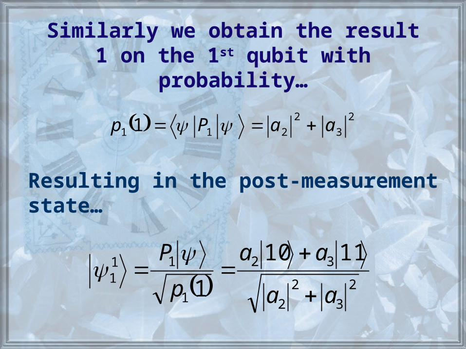
Similarly we obtain the result 1 on the 1st qubit with probability…

2

3

2

211 1 aaPp

Resulting in the post-measurement state…

2

3

2

2

32

1

111

1110

1 aa

aa

p

P

In the same way for the second qubit…

,1

,0

2

3

2

12

2

2

2

02

aap

aap

2

3

2

1

3112

2

2

2

0

2002

1101

1000

aa

aa

aa

aa

Consider the entangled 2-qubit

2/1100

2/1100

2

1 ,0 ,0 ,

2

13210 aaaa

We consider with amplitudes

After applying Quantum Measurement Techniques

2

11010 2211 pppp

11 ,00 12

11

02

01 vvvv

the post measurement states are

(A Perfectly Correlated Measurement)

The probabilities for each state for each qubit are all 1/2

Conclusion

• Brief History of Quantum Mechanics• Tools Of Linear Algebra

– Complex Inner Product Spaces– Linear and Unitary Operators– Projections– Tensor Products

Conclusion Cont.

• Dirac Bra-Ket Notation– Inner and Outer Products– Completeness Equation– Outer Product Representations– Projections– Computational Bases

Conclusion Cont. (again)

• Mathematical Model of Quantum Mech.– Quantum States– Postulates of Quantum Mechanics– Product vs. Entangled States

Where do we go from here?

• Quantum Circuits• Superdense Coding and Teleportation

Bibliography

http://en.wikipedia.org/wiki/Inner_product_space

http://vergil.chemistry.gatech.edu/notes/quantrev/node14.html

http://en2.wikipedia.org/wiki/Linear_operator

http://vergil.chemistry.gatech.edu/notes/quantrev/node17.html

http://www.doc.ic.ad.uk/~nd/surprise_97/journal/vol4/spb3/

http://www-theory.chem.washington.edu/~trstedl/quantum/quantum.html

Gudder, S. (2003-March). Quantum Computation. American Mathmatical Monthly. 110, no. 3,181-188.

Special Thanks to:

Dr. Steve Deckelman

Dr. Alan Scott

presented by: erik cox, shannon hintzman, mike miller, jacquie otto, adam serdar, lacie zimmerman

Documents